Metrohm Vision User Manual

Download

NIRS Vision – Diagnostics

Manual

8.105.8013EN

Metrohm AG CH-9100 Herisau Switzerland Phone +41 71 353 85 85 Fax +41 71 353 89 01

info@Metrohm.com www.Metrohm.com

NIRS Vision – Diagnostics

Manual

8.105.8013EN 2014-06-20 / fpe

Teachware Metrohm AG CH-9100 Herisau

teachware@Metrohm.com

Although all the information given in this documentation has been checked with great care, errors cannot be entirely excluded. Should you notice any mistakes please send us your comments using the address given above.

▪▪▪▪▪▪▪

Table of contents

1 Overview ........................................................................................................................ 5

1.1 Vision Diagnostics Screen Display ................................................................. 9

2 Performance Test ......................................................................................................... 12

2.1 Overview .................................................................................................... 12

2.2 Noise Test ................................................................................................... 14

2.3 Bandwidth: Wavelength Accuracy and Precision ........................................ 16

2.4 Model 5000 and 6500 ................................................................................ 16

2.5 Wavelength Accuracy / Precision Measurement on the XDS ....................... 17

2.6 Operational Qualification ............................................................................ 18

2.7 Performance Test Timer.............................................................................. 19

3 Wavelength Certification .............................................................................................. 20

3.1 Run Wavelength Certification ..................................................................... 20

3.2 Setting up a User-Defined Wavelength Standard ........................................ 23

4 Reference Standardization ........................................................................................... 24

4.1 Creating a Reference Standard ................................................................... 25

4.2 Loading a Reference Standard .................................................................... 28

4.3 Reset Reference Standard ........................................................................... 28

5 Create Blank Correction ............................................................................................... 29

6 Window Correction ...................................................................................................... 31

7 Low-Flux Test ............................................................................................................... 32

8 Instrument Self-Test ..................................................................................................... 34

9 Wavelength Linearization ............................................................................................. 35

9.1 Wavelength Linearization on Model 5000 and 6500 .................................. 35

9.2 Wavelength Linearization on XDS Instruments ........................................... 36

9.3 Special Note on Wavelength Linearization of Process Instruments ............. 37

10 Gain Adjust ................................................................................................. 38

10.1 Autogain ..................................................................................................... 38

10.2 Manual Gain ............................................................................................... 39

11 Photometric Test ........................................................................................ 40

12 IPV Setup .................................................................................................... 44

13 Diagnostic Database ................................................................................... 46

13.1 View Diagnostic Database .......................................................................... 46

13.2 Backup and Restore Diagnostic Database ................................................... 46

13.3 Archive Diagnostic Database Information ................................................... 47

13.4 Export and Import Diagnostic Database Information .................................. 48

13.5 Diagnostics Timers ...................................................................................... 49

13.6 Maintenance Log ........................................................................................ 51

13.7 Show Status ................................................................................................ 52

14 Instrument Configuration ........................................................................... 53

15 Instrument Calibration (XDS instruments only) ........................................... 54

16 USP Tests .................................................................................................... 56

▪▪▪▪▪▪▪

16.1 Full USP Test .............................................................................................. 56

16.2 USP Noise .................................................................................................. 57

16.3 Usp Low-Flux Noise Test ............................................................................ 57

16.4 Usp Wavelength Accuracy .......................................................................... 58

USP Photometric Linearity Test ................................................................................... 59

16.5 Photometric Linearity Setup ....................................................................... 61

16.6 Show USP Test Results ............................................................................... 61

17 Troubleshooting Tips ................................................................................. 62

17.1 Instrument Error: Run Wavelength Linearization........................................ 62

17.2 Weak Signal ............................................................................................... 62

17.3 Increasing Noise ......................................................................................... 63

▪▪▪▪▪▪▪

1 Overview

Vision provides a complete set of diagnostics functions to test whether the Metrohm instrument performs according to the manufacturer’s specifications. Instrument performance tests verify the reliability of NIRSystems spectrophotometers, which insures the linearity, limits of detection, and precision of NIR methods.

The Vision software drives all Metrohm spectrophotometers. There are differences in the performance and diagnostic testing associated with the instruments. For the Model 5000 and 6500 instruments, please refer to the Instrument Performance Test Guide for further explanation on performance tests. For the XDS instruments, there are additional set-up and evaluation diagnostics, with slight differences for the various analyzers. Proper application of these tests is recommended to ensure instrument matching and the seamless transfer of calibration methods developed on the XDS. There are specific requirements for process instruments as well. Refer to the instrument manual for your particular instrument. For tests that require the use of external standards, be careful that the correct standards are used depending on your instrument type. Please be sure to follow the correct section in this manual for your particular instrument type.

More detailed information about XDS Analyzers can be found in the installation and user manuals provided with the analyzer:

• 8.921.8001EN Manual NIRS XDS RapidContent and RCA Solids Analyzer

• 8.921.8004EN Manual NIRS XDS SmartProbe Analyzer

• 8.921.8005EN Manual NIRS XDS RapidLiquid Analyzer

• 8.921.8006EN Manual NIRS XDS Interactance OptiProbe Analyzer

• 8.928.8001EN Manual NIRS XDS Process Analyzer – MicroBundle

▪▪▪▪▪▪▪

Instrument model

Module

Standards

Numbering

5000 or 6500

Liquid Analyzer, Sample

AP-0220 Transmission

TSS3xxxx

5000 or 6500

InTact

AP-0230 Single Tablet

TSS2xxxx 5000 or 6500

MultiTab

AP-0240 Multi Tablet

TSS2xxxx

XDS

RCA, Rapid Solids Module,

XC-1010 Reflectance

RSS1xxxx XDS

Rapid Liquid Analyzer

XC-1310 Transmission

TSS3xxxx

5000 or 6500 RCA, DCA, Smart Probe,

Sample Transport (Reflectance), etc.

Transport (Transmission.)

Smart Probe, OptiProbe (reflectance)

NIST traceable standards for use on the Metrohm NIR spectrophotometers

AP-0200 Reflectance Standards

Standards

standards

RSS1xxxx

▪▪▪▪▪▪▪

Vision SP includes enhanced Diagnostics, designed specifically to meet the needs of users in regulated industries who must maintain complete instrument records of performance over time, including conformance to photometric and\ wavelength standards. Among the features are the following:

• Diagnostic Database structure to support multiple instruments, multiple sampling configurations

• Built-in table with acceptance specifications for all current, standard Metrohm NIRSystems instrument and sampling modules, applied by instrument configuration

• Recallable test results, with control charts to show performance changes over time

• Control charts offer both calculated control limits and manufacturer’s tolerances

• A unique screen display to show data in various formats, permitting enlargement of each area

for better interpretation

• Test timer supports all available tests, prompts operator when tests are due

• Instrument Self-Test (similar to NSAS Self-Test)

• Photometric Certification tests for supported reflectance and transmission standards

• Wavelength Certification for supported (and user-defined) wavelength standards

• Instrument Performance Verification (IPV) for regular user tests of photometric performance

• Low-Flux Test in support of pharmaceutical requirements

• Reference Standardization for users of reflectance instruments

• Instrument maintenance log with comment fields

• Blank Correction (for XDS transmission measurements)

• Instrument Calibration (for ensuring calibration transfer between XDS instruments)

• Window Correction (For XDS process systems)

• USP tests including Noise, Low-Flux Noise, Wavelength Accuracy and the Photometric

Linearity Test – with results displayed according to the USP chapter <1119>.

▪▪▪▪▪▪▪

The tests in this manual are listed in the order in which they appear in the Vision software drop down menus. More information on the order of running tests can be found in the Installation and user manuals for the particular instrument being used.

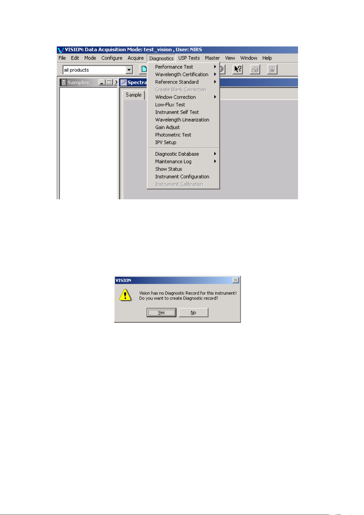
When an instrument is first connected to Vision, Vision will determine whether there is a diagnostic record for this instrument configuration. In order to establish the correct instrument record in the Diagnostic Database, choose the option to create the diagnostic record when the initial screen appears telling that a Diagnostic Record does not exist for this instrument.

Saying “yes” will not initialize the testing, but will enter the instrument configuration information in the Diagnostic Database.

An instrument configuration is defined as a given monochromator and it assembled sampling components, including fiber-optics, if used. Where fiber-optics are used, the sampling tip type, fiber material and fiber length all constitute part of the monochromator configuration.

For most users with a single instrument, the configuration may never change, and is thus not an overriding issue in diagnostics. Other users may operate several instruments from one computer, or may change sampling modules based upon the sample characteristics. Diagnostic test results must be maintained separately for each configuration, to assure use of correct tolerances, and for correct information in control charts.

▪▪▪▪▪▪▪

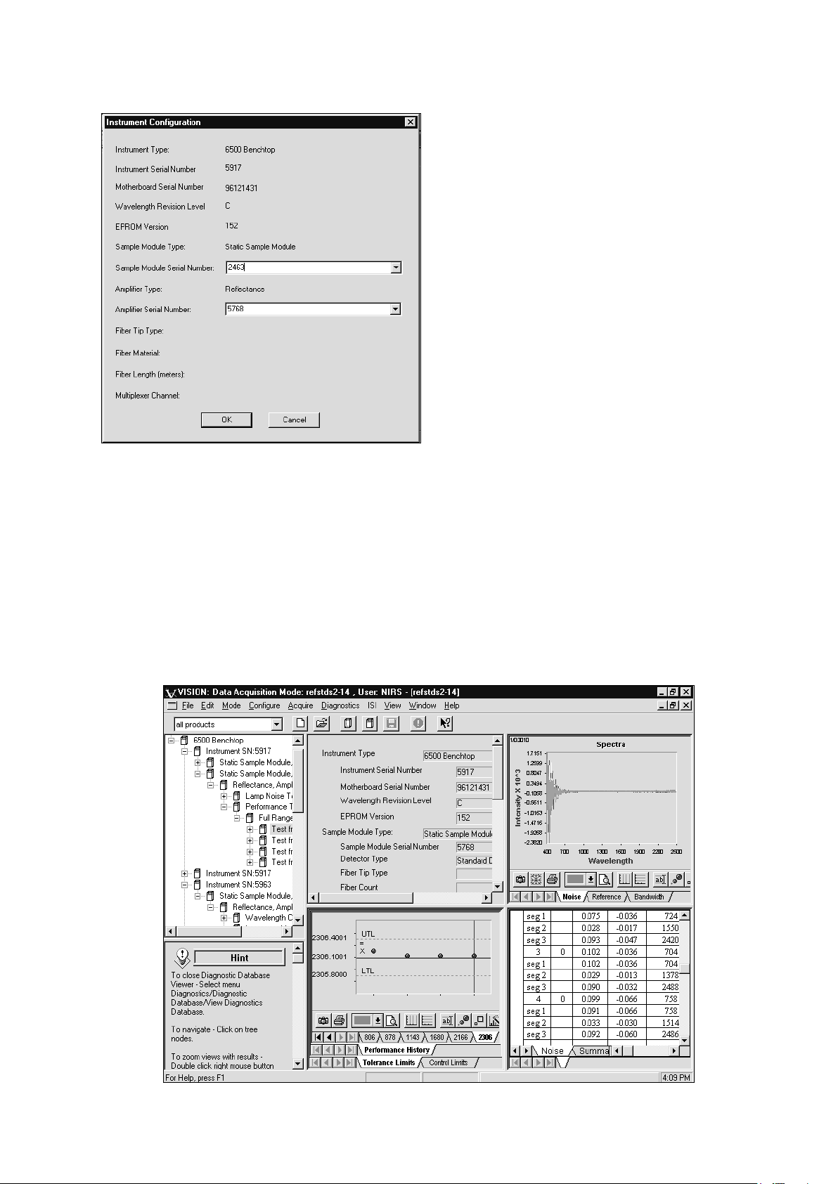
Confirmation of Instrument configuration

If the instrument configuration is not

recognized upon connection, Vision prompts for full instrument configuration information, including serial numbers of the monochromator and modules. A typical screen for a simple configuration is shown.

For instruments with fiber-optic sampling devices, the tip, material, and fiber length are required. For multiplexed process systems, enter this information for each channel.

Vision builds a database of diagnostic information for the instrument. It is vital to enter correct information, to assure application of correct tolerances for tests and for accurate tracking of test results.

Tools for export, import and archiving of information in case of computer upgrades, changes, or instrument moves, are explained under Diagnostic Database.

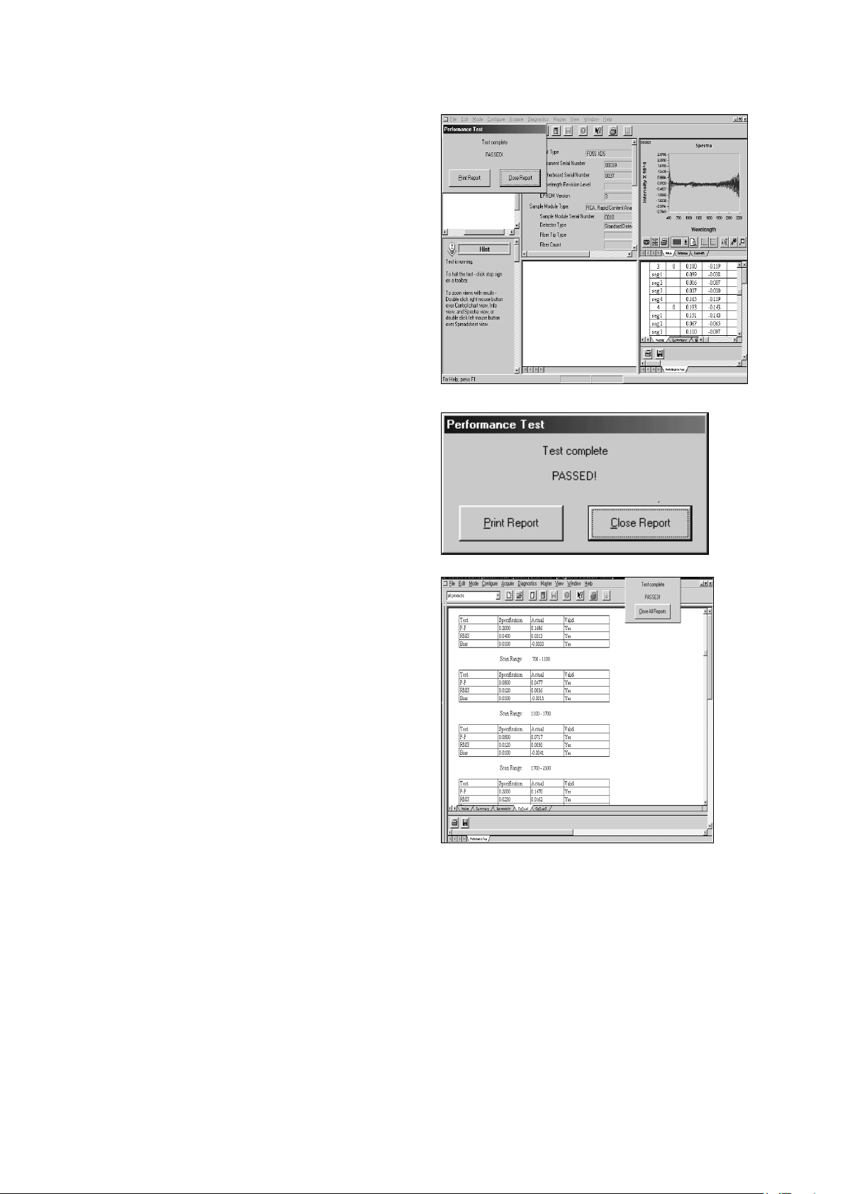
1.1 Vision Diagnostics Screen Display

Vision Diagnostics use a split-screen display to provide as much information as possible to the user. This is a screen displayed during the Performance Test; other tests use the same display format. Because each part of the screen may be used at different points during the test, all are displayed in small size, and can easily be enlarged for better viewing. Each part of the screen is discussed in the section following.

Vision Diagnostics Screen Display

▪▪▪▪▪▪▪

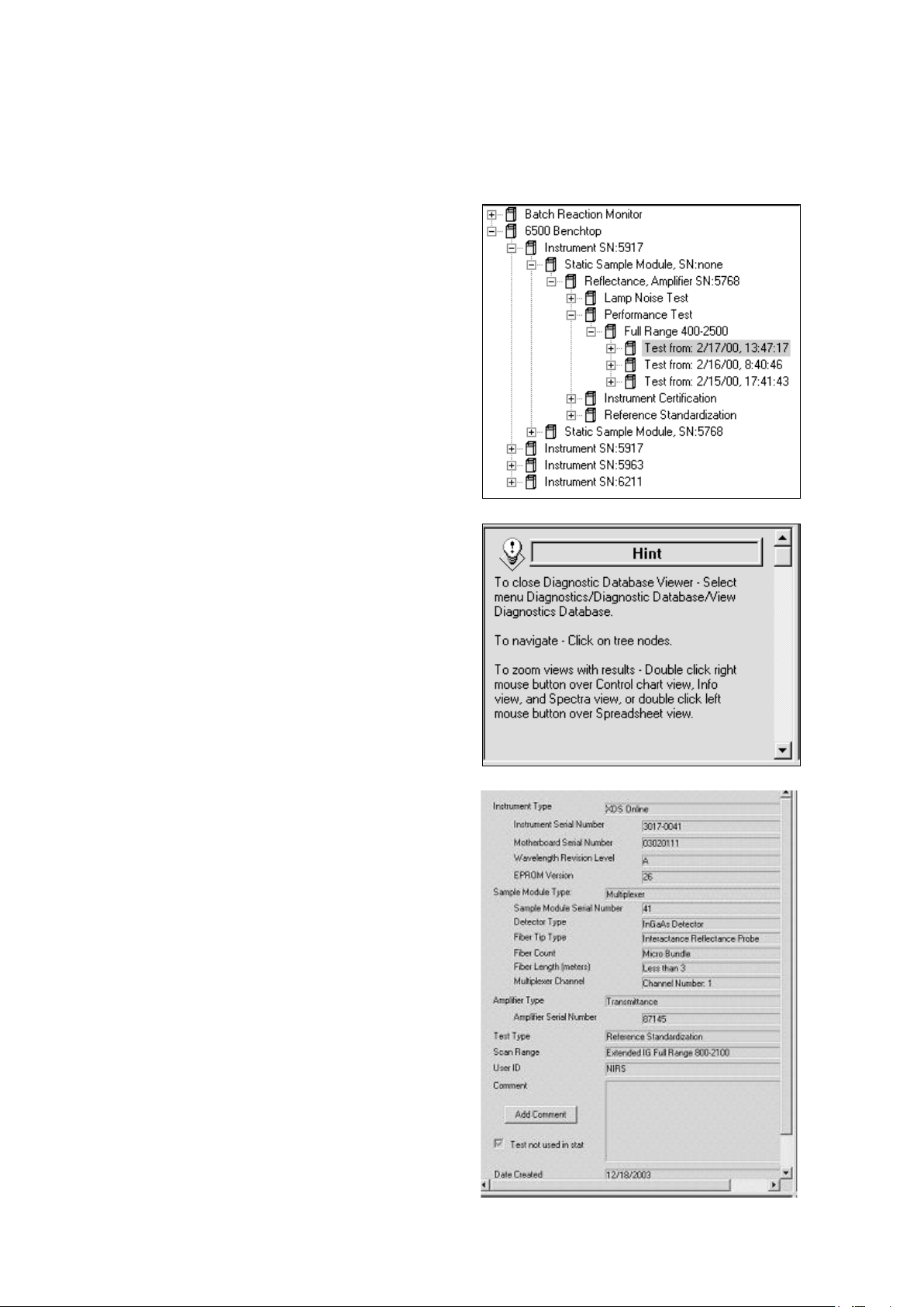
The instrument selection tree lists all instruments for

The Hint box tells how to zoom each of the four

The user may size the boxes manually using the mouse to move the partitions left, right, up or down. The configuration box, spectrum box, and control chart boxes are all a double right-click to enlarge or restore. After enlargement, double-click is repeated to return to the original display mode.

which information is stored in the database.

Click on the “+” sign beside each node to see all items underneath. Each instrument lists all stored configurations, tests, along with the date and time of each test.

boxes, along with other useful suggestions.

The hint box is useful throughout Vision, and suggests steps to the user to help navigate Vision most efficiently.

The upper middle box lists the full instrument configuration. The box shown is for a process system, which includes fiber-optic probes.

With process systems, the “Sampling Module Type” is integral to the instrument, and carries the same serial number as the instrument.

Comments can be added for individual test results by clicking on the “Add Comment” combo box.

The upper right box shows spectra where applicable. In this case, noise spectra for a tested instrument are displayed.

▪▪▪▪▪▪▪

Other information displayed is the reference scan, or

the polystyrene/didymium spectra used for

The lower left quadrant shows control charts, when The lower right box shows tabular data. Click on the

wavelength linearization.

A left-click on the spectrum gives a cursor which gives wavelength and absorbance information for a selected spectrum, as throughout Vision. The selected spectrum is identified by a color bar above the wavelength and absorbance.

When this window is active the user may click on the camera icon to copy the spectral image to the clipboard. The user may click on the printer icon to print spectra.

enough data is stored for a given instrument configuration to plot control charts.

The top row of tabs is for selection of test (RMS noise is shown). Other choices are Peak-to-Peak, Bias, Bandwidth, and the Wavelength Linearization peaks.

The bottom tabs select between tolerances or control limits. Control limits are calculated on one specific instrument and give an excellent insight into any changes that may occur over time. Trends may be noted and acted upon before the parameter has gone outside of tolerance.

tabs at the bottom to see each view. The options are Noise, Summary, Wavelength, and OpQual (Operational Qualification). The OpQual tabs provide a summary of the actual instrument performance versus specification values.

A double right click on the table takes the user to Formula One Worksheet mode, which permits easy cut-and-paste export of results to other Windows™-based programs. When finished with Formula One, click on the “X” to close.

▪▪▪▪▪▪▪

Select Performance Test from the Diagnostics

All diagnostic test results are stored in the

2 Performance Test

2.1 Overview

Performance Test is a comprehensive test of instrumental performance, and is the final assurance that the instrument is ready to run samples. The key items verified during this test are:

• Instrument Noise in several wavelength regions depending on the instrument type and configuration

• Internal Wavelength Performance (wavelength positions on non-traceable, internal reference materials)

• Internal Wavelength Precision (Repeatability)

• NIR Gain

• Visible Gain (where applicable)

menu. Click on Run Performance Test. The test will commence immediately.

Performance Test takes approximately 15-25 minutes to run depending upon settings, instrument status and instrument type.

The test co-averages the results of 32 scans, irrespective of DCM settings for the number of scans. This assures correct application of acceptance specifications and consistent comparison of test results to initial factory test results.

The samples per test are set to a default of 10, but this can be changed under Performance Tests, Configure Test Parameters. Use the default settings unless there is a compelling reason to change them.

Diagnostic Database, regardless of which project the user is logged into while performing the tests. The user may store results in Excel format using the drop-down menu shown. Test results in the Diagnostic Database can be recalled at a later time.

▪▪▪▪▪▪▪

As the test runs, a screen like that shown to the

left is displayed. When finished, a message box is

Before clicking “Close All Reports”, the user is

To enlarge the tabular display of results, place

displayed to indicate test completion and status.

At the end of the Performance Test, all measured values are compared with acceptance criteria stored in Vision. If all results meet acceptance criteria, the test is successful and this dialog box is displayed.

directed to the tabular display in the lower right quadrant.

the cursor over the tabular display in the lower right quadrant and double-click twice. Now click on the OpQual tab, near the bottom of the screen to see a summary of noise test results.

The OpQual tab brings up the display shown. This shows results of the Noise Test for each of the up to four wavelength regions. The results are shown along with the specification values and a column to show if the test results are valid.

For each wavelength region, results are given for:

• Peak-to-Peak Noise (P-P)

• Root-Mean-Square Noise (RMS)

• Bias (A measure of baseline energy changes)

Each of these parameters is described in more detail in the next section and in the Instrument Performance Test Guide supplied with the Metrohm instrument. If the test is reported as “Passed” the user may proceed with sample analysis.

▪▪▪▪▪▪▪

A note on Wavelength Linearization:

Sometimes when initiating Performance Test, Vision will report “Instrument Error: Run Wavelength Linearization”. The error report is posted near the end of the first set of 32 co-averaged scans, as Vision processes the data. This error occurs when an instrument configuration has been changed, the lamp is not on, the reference is not in the correct position, or due to a beam blockage. A troubleshooting table is provided at the end of Diagnostics to assist you in solving this issue.

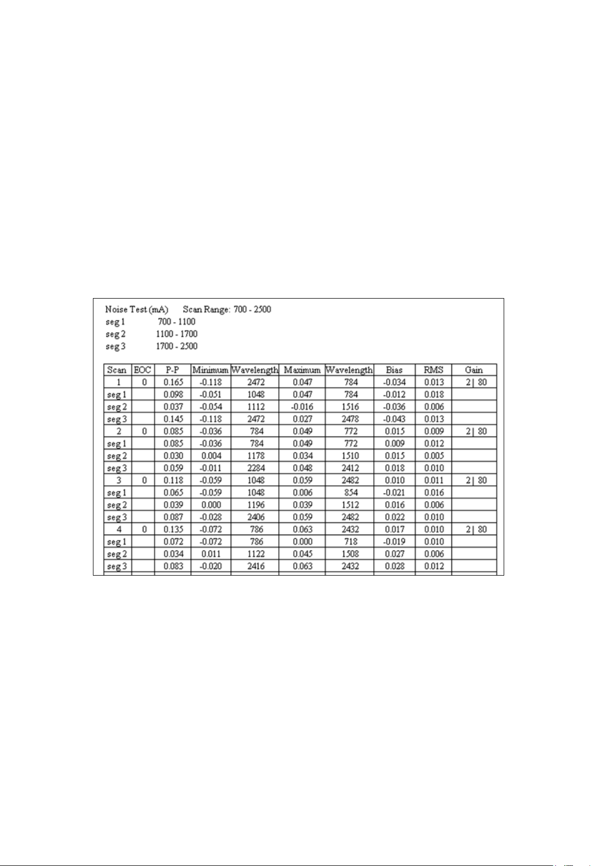
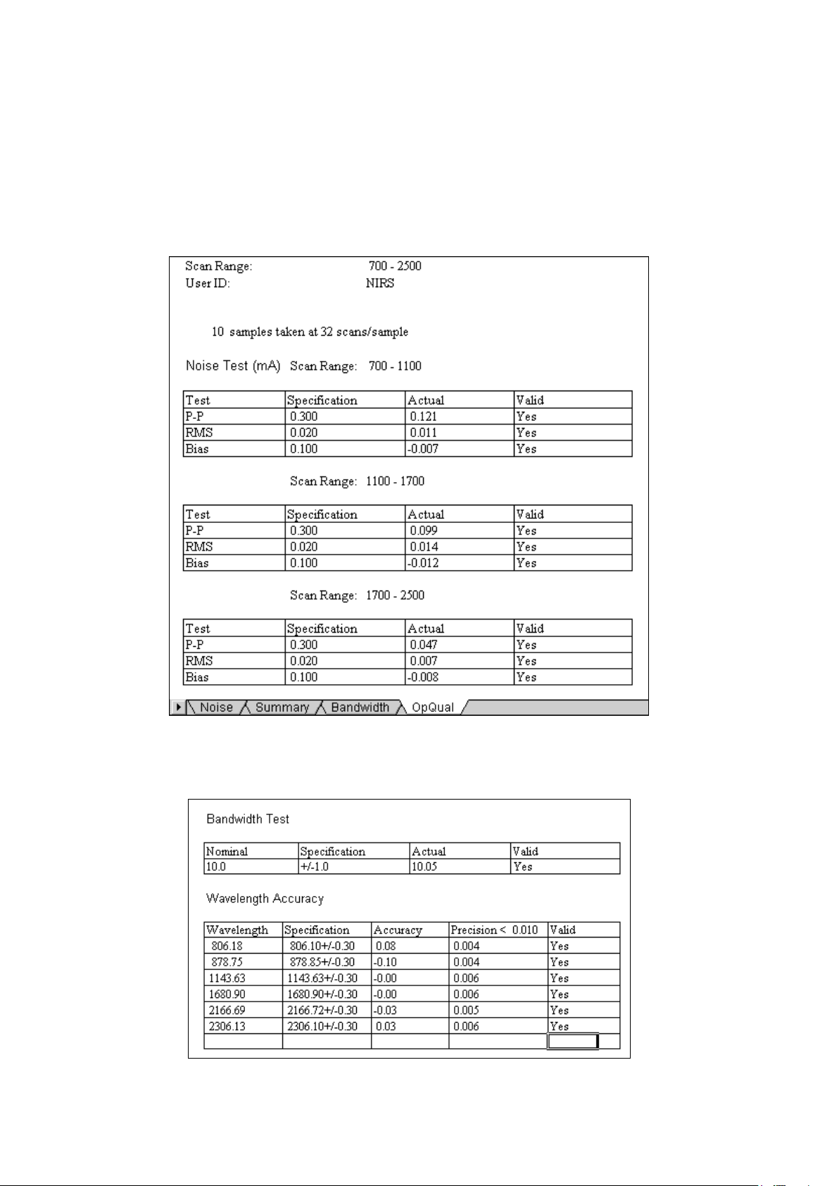
2.2 Noise Test

The tabular output of the instrument Noise portion of Performance Test provides a wealth of information about the instrument. Instrument noise should appear as random spectral variability. Structure in the noise spectrum or high noise is often caused by changes in environment but also may be indicative of instrument problems. The Noise Test is the most sensitive diagnostic test used to determine instrument performance. The display provides information about noise and amplifier gain.

Instrument Noise (Displayed at lower right quadarant during Performance Test)

Vision breaks each instrument test up into segments (wavelength regions), based upon the instrument configuration. Acceptance specifications are applied to each segment. Segments can be adjusted by the user under Tests Params (under Data Collection Method) prior to acquisition of any spectra. Unless there is a reason to change segments, the user is encouraged to use the defaults.

Laboratory instruments generally use a ceramic reference in reflectance, or air in transmission. Process instruments offer the option of reference vs. reference, sample vs. sample, or sample vs. reference. Each result column in the noise test is explained:

SCAN#

Identifies which of the 10 sets of sample scans is being reported. A sample scan is defined as 32 sets of co-averaged reference vs. reference scans for a laboratory instrument.

▪▪▪▪▪▪▪

EOC

End of convert. Communications failures during the instrument scan and with the computer are reported here. This number should be zero, and if not the source of communication errors should be investigated. Occasionally, EOC failures are due to random electrical noise or unexplained disturbance, and if not frequently repeated they are not considered a problem.

P-P

Peak-to-Peak noise is the difference between the largest and smallest value in the noise spectrum. (There may be a round-off error of .001 due to the mathematical algorithm.) The unit of measure is milliabsorbance units, or one-thousandth of one absorbance unit. For example, .139 equals 0.000139 absorbance units. The number may also be expresses verbally as microabsorbance units, or “139”. Peak-to-peak noise may be thought of as the greatest variation from one scan to the next scan of the noise spectrum across all measured wavelengths.

Minimum

This is the highest intensity negative peak height, in milliabsorbance units, of the noise spectrum. The wavelength where the minimum occurs is reported in the next column.

Wavelength

The wavelength where the peak minimum occurred.

Maximum

This is the maximum peak height, in milliabsorbance units, of the noise spectrum. The wavelength where the maximum occurs is reported in the next column.

Wavelength

The wavelength where the peak maximum occurred.

Bias

The bias is the average absorbance value of all points in the noise spectrum. Immediately after the instrument is turned on, the bias is quite high, and as the instrument warms up, bias settles to near zero with slight random excursions above and below. In normal operation, fully warmed-up, the bias should run in a range of +/-0.100 milliabsorbance units.

RMS

The Root Mean Square of the noise across the full spectral region in milliabsorbance units is reported. Each sampling configuration has acceptance specifications programmed in Vision. These are applied automatically. As with peak-to-peak noise, RMS is commonly referred to in microabsorbance units.

(One-million

of an absorbance unit.) In this case, 20 microabsorbance units is equivalent to 0.020

milliabsorbance units.

Gain

The “gain factor” for Autogain amplifiers is shown. For full-range instruments the NIR gain is shown first, then the visible gain. Metrohm’ instruments use a system of gain optimization called “AutoGain,” which uses the first scan of each data collection to adjust the gain level for the best resolution of signal.

The detector picks a gain factor to optimize signal. The gain factor depends upon the sample absorbance, requiring no user adjustment. This can be helpful when troubleshooting. For example, if

▪▪▪▪▪▪▪

the instrument reference is not in place, gain factors may climb to the maximum value, and may also explain why RMS noise and P-P are outside of bounds.

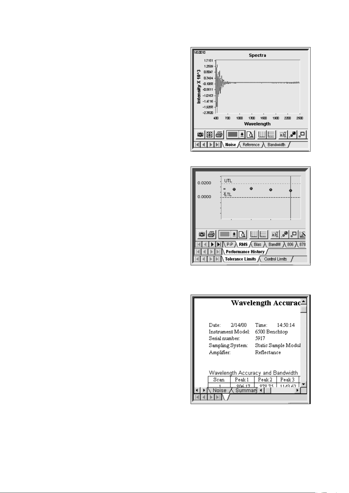
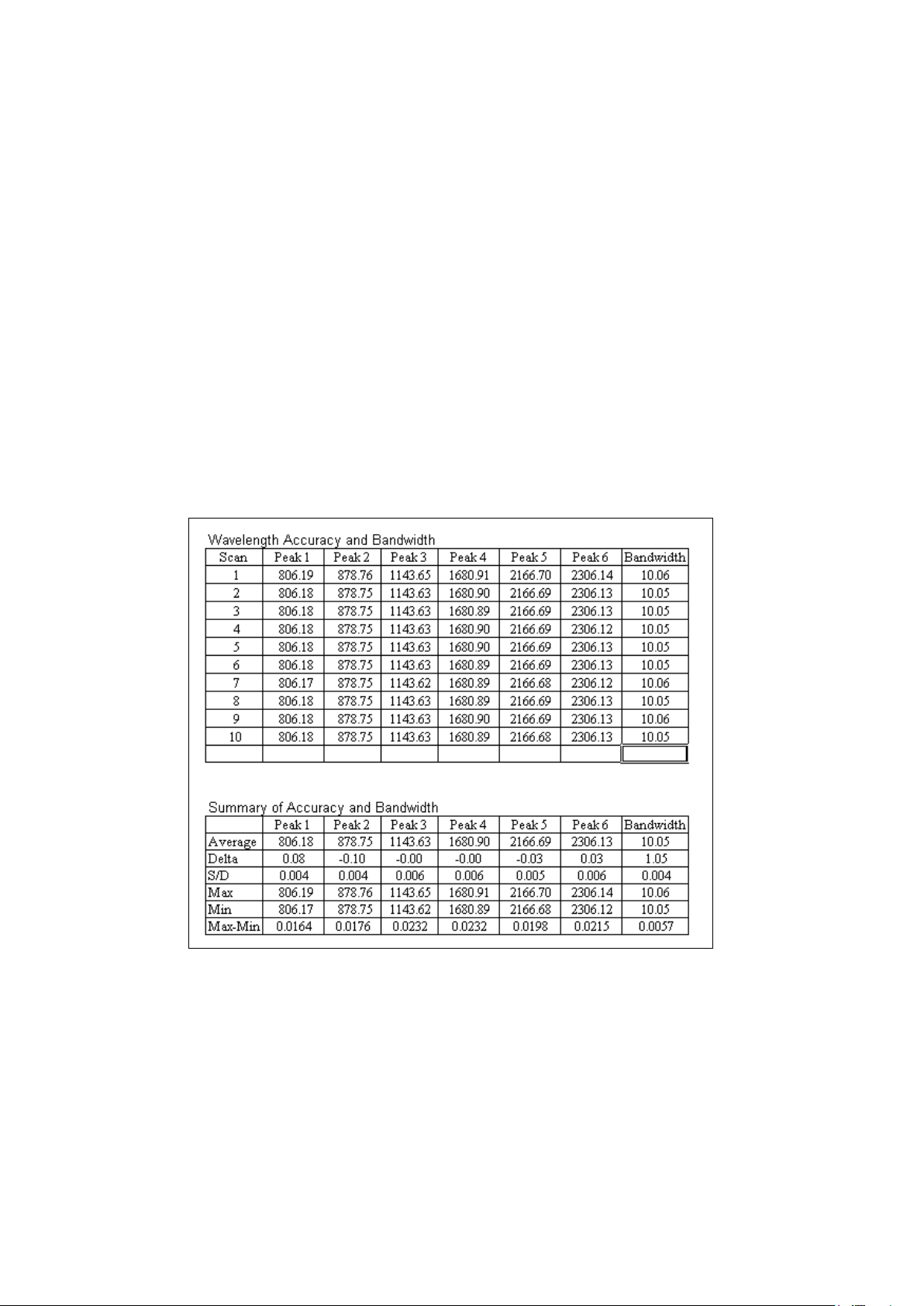
2.3 Bandwidth: Wavelength Accuracy and Precision

Bandwidth is measured during the Performance Test on non-XDS instruments and during the Wavelength Certification test for XDS instruments. Metrohm instrument contains internal wavelength reference materials, which are used as a means to maintain monochromator wavelength measurement. These internal wavelength materials are protected and are moved by software command, transparent to the user. When Performance Test is run, the relative wavelength positions and repeatability of these wavelength materials are monitored and reported.

2.4 Model 5000 and 6500

The Bandwidth tab shows instrument bandwidth as well as wavelength accuracy and precision. In the NIR region, an internal polystyrene reference is analyzed by transmission measurement under software control. 10 replicate scans of the polystyrene standard are used to calculate these parameters.

The polystyrene absorbances which nominally occur at 806.10, 878.75, 1143.63, 1680.90 2166.72 and 2306.10 nm (Rev. C) are used to calculate wavelength accuracy and precision. A peak-finding algorithm is applied to the polystyrene spectra to determine the peak maxima. The average peak position obtained for 10 replicates determines the wavelength accuracy, and the standard deviation of those values determines measurement precision.

Delta is the difference between the accepted nominal values, and those reported by the instrument. The specification for reported vs. nominal is +/- 0.30 nm (+/- 0.50 for process instruments). Therefore, any peak found to be within 0.30 nm is considered acceptable. The software flags any peak outside the acceptance range and suggests that Wavelength Linearization be performed.

S/D is the standard deviation of the 10 replicates. This measures the stability of peak positions and

▪▪▪▪▪▪▪

bandwidth. With respect to peak position, the specification on S/D is 0.015 nm or less, depending upon instrument model and type.

The instrument bandpass (bandwidth) is calculated using the ratio of the absorbance at the polystyrene peak at 2167 nm and the valley at approximately 2154 nm (after an offset correction.)

The S/D test is also run in the 400-1100 area of the spectrum on models 5500 and 6500. In this area, didymium/polystyrene is used for two of the peaks, at 806.10 and 878.85 nm. Bandwidth is not calculated in the 400-1100 nm area.

Process instruments (and certain laboratory instruments) cannot use the polystyrene peak at 2306.10 nm due to attenuation of the signal in the fiber-optics, or limitations in wavelength range. On such instruments the tests will not report values for the 2306.10 peak, and will perform wavelength tests on peaks within the wavelength response of the instrument.

Note: Wavelength positions are empirically determined, and have been set based upon the best measurements possible given the technology available. As instrumental or standardization breakthroughs lead to greater precision in setting nominal peak positions, Metrohm reserves the right to issue revised nominals.

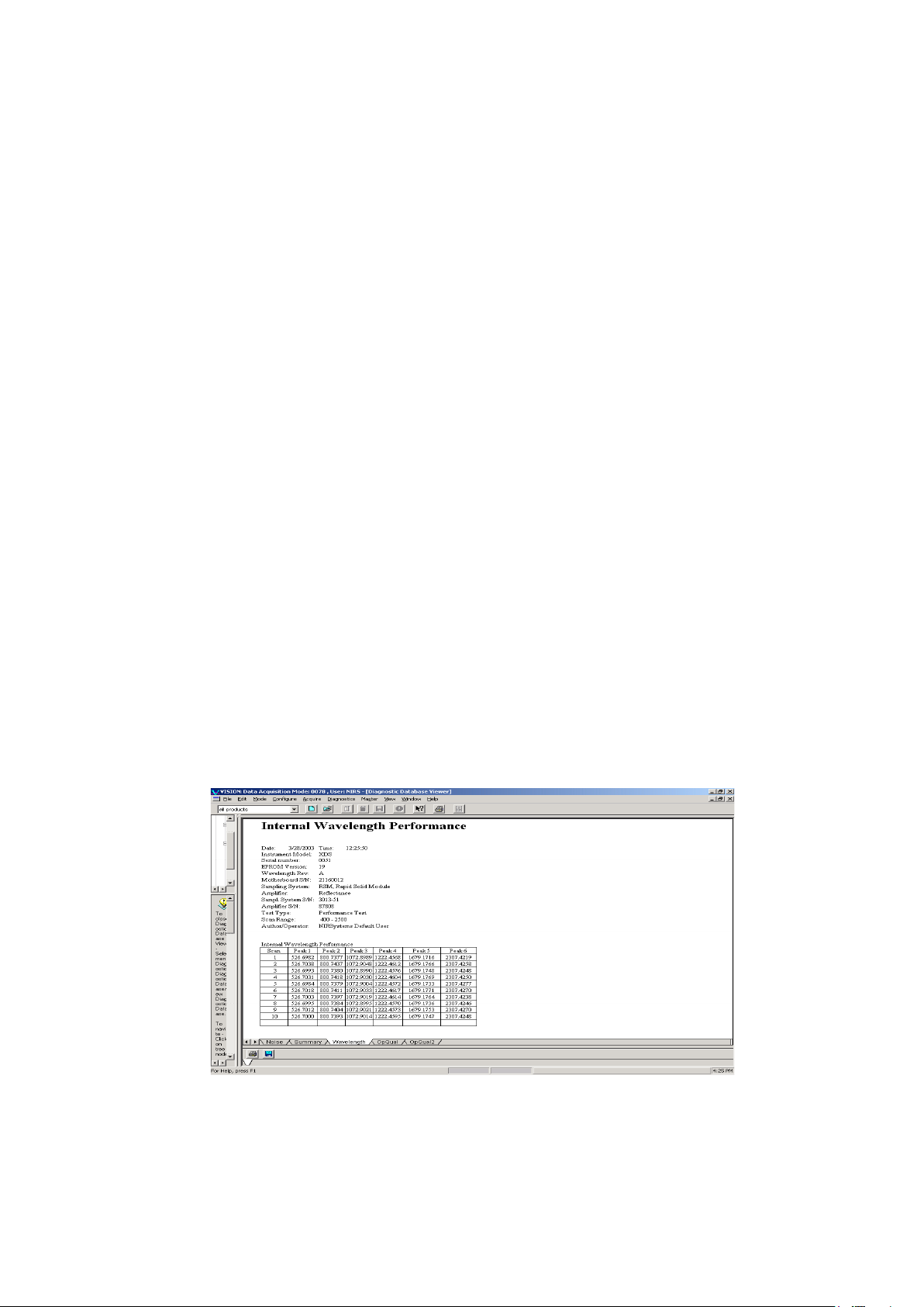
2.5 Wavelength Accuracy / Precision Measurement on the XDS

The XDS instrument, like the model 5000 and 6500, uses an internal wavelength reference material. When Performance Test is run, the relative wavelength positions and repeatability of these wavelength materials are monitored and reported. The internal standard for the XDS is comprised of polystyrene, erbium oxide and samarium oxide and six peaks across the range from 500-2310nm are used to determine the internal wavelength performance of the instrument.

Note that these internal wavelength materials need not be precisely on the assigned nominals. These nominals are arbitrary. The internal wavelength materials are a method to assure stable readings on the external wavelength standard, measured at the sample plane during Instrument Calibration and Wavelength Certification.

▪▪▪▪▪▪▪

2.6 Operational Qualification

A summary of noise results is available in the OpQual (Operational Qualification) screens. This screen gives specifications (for a given instrument configuration), the average of measured values, and an indication of whether the result is valid for that configuration. The measured values are the average result for 10 sets of scans, covering each wavelength region. Many users find this screen easier to interpret, and more concise, than the tabulated data for each set of scans.

Operational Qualification Summary Screen: Noise Test

The OpQual2 tab contains summary information on wavelength accuracy and precision. For Model 5000 and 6500 instruments it also contains information on the bandwidth, as shown:

Operational Qualification Summary Screen: Bandwidth, Wavelength Results

▪▪▪▪▪▪▪

2.7 Performance Test Timer

The Performance Test Timer permits the user to

automatically set the instrument to run the Performance Test unattended. It may be set for a time interval or on a daily basis at a preset time. Use military time for time of day, i.e., 20:45 for 8:45 p.m. Be sure the instrument is left on with the reference in the correct position for Performance Test.

If the specified time has passed, Performance Test begins immediately upon successful connection with the instrument.

Note that there is a Diagnostic Timer under Diagnostic Database, where many functions can be set up for timed testing and storage of results. See Diagnostic Database for more information.

▪▪▪▪▪▪▪

Click on Diagnostics, Wavelength

It may be read using the A: drive, or may be

3 Wavelength Certification

Wavelength Certification uses an external standard, with known peak positions, to verify the wavelength scale of the instrument. The program is designed to run a certified Wavelength Standard available from Metrohm. For reflectance measurements the standards are traceable to SRM-1920, supplied by NIST. The standard for XDS reflectance instruments is SRM-1920 plus talc. For liquid transmission systems the wavelength standard is polystyrene-didymium (XC-1310/XC1320) or SRM-2035 (XC-1330). Vision also offers the option of a user-defined wavelength standard, with appropriate tools for peak-finding and tolerances.

3.1 Run Wavelength Certification

Certification, Run Wavelength Certification.

The Number of samples should be 10, as shown. Select the correct standard for the instrument type being used from the drop down menu.

Click “OK” when ready.

Vision requests the Standard File for the wavelength standard. This file is located on the diskette or CD packed with the 6-piece standard set.

copied into the C:\Vision directory as shown here.

The file name will be similar to that shown below.

Click “Open” to proceed.

▪▪▪▪▪▪▪

RSS1xxxx

Reflectance

TSS2xxxx

Tablets (MultiTab,

Transmission

When prompted by the software, insert the

The wavelength standard is scanned, and a

400 600 800 1000 1200 1400 1600 1800 2000 2200 2400

-0.42

-0.39

-0.36

-0.33

-0.30

-0.27

-0.24

-0.21

-0.18

-0.15

-0.12

-0.09

-0.06

-0.03

0.00

0.03

0.06

Spectrum of SRM 1920

Wavelength (nm)

Absorbance log(1/R)

File

Sample Type Detector

Name

InTact)

TSS3xxxx Transmission Transmission

The standard file contains spectra of standards taken on the appropriate Metrohm master instrument. It is important to use a certified wavelength reference that has been checked and verified for correct wavelength response.

appropriate standard into the sample drawer. The label should face the user when inserting the standard.

If the standard file chosen is for the wrong type of standards, Vision will inform the user of the error. Since Wavelength Certification is run regularly, the user may copy the standards file from the diskette to the C:\Vision directory of the computer for simplicity. This file must be updated upon recertification of the standard set.

peak-finding algorithm locates the peaks produced by the standard material. The horizontal axis is wavelength, and the vertical axis is absorbance. These peaks must be measured within the tolerance defined in Vision to be considered valid or acceptable.

After the test is complete, a spectrum of the standard is shown in the upper right quadrant of the screen. An example of the spectrum of SRM-1920 measured on an RCA is shown.

▪▪▪▪▪▪▪

A tabular report is shown in the lower right

quadrant, giving each peak, its nominal position and its measured position. The difference from nominal and the repeatability of position are calculated. This is a sample report for an XDS analyzer.

This report is stored in the Diagnostic Database and can be accessed from the Diagnostic Database Viewer at a later time.

For XDS instruments, the Wavelength Certification also tests certain measured instrument profile peaks in the wavelength standard. These peaks are used to set the “Instrument Wavelength Profile,” and one peak is used for bandwidth calculation.

When running Wavelength Certification on the XDS, the test may pass, but give a recommendation to re-run the instrument calibration to improve instrument performance. For the XDS, there is a tab at the bottom of the test results for the Instrument Calibration Verification results, which has much tighter tolerances. If the peak positions measured during the Wavelength Certification are outside of these tolerances, yet still acceptable for Wavelength Certification, it is recommended that the user re-run Instrument Calibration to ensure instrument matching and seamless calibration transfer.

If Wavelength Certification fails on an XDS instrument, run Instrument Calibration under Diagnostics, then repeat the Wavelength Certification Test. If it fails on model 5000 or 6500 instruments, run Wavelength Linearization under Diagnostics, then repeat the Wavelength Certification. If the system fails the test again, contact Metrohm Technical Support.

▪▪▪▪▪▪▪

3.2 Setting up a User-Defined Wavelength Standard

Click on “Setup Custom Wavelength Standard” to create a user-defined wavelength standard to be used to verify wavelength axis repeatability. (The material must have sharp, well-defined peaks, and be very stable to serve as a wavelength reference.) Name the standard. Collect a reference scan on the instrument reference, typically a ceramic for reflectance, air for transmission. Scan the user-defined wavelength standard when prompted. An example is shown for illustration:

Set up Custom Wavelength Standard

To select peaks, click on the vertical line, draw it to a peak, and then release the mouse button. A small “+”denotes the peak. A peak-finding algorithm is applied for accuracy in peak assignment. The Peak Position is shown in the table. Up to 16 peaks may be selected. The default tolerances are +/- 0.15nm, which may be edited by the user. To delete a peak, highlight the box in the table and click Del. When finished, click “Done”.

To use the custom wavelength standard, select Run Wavelength Certification. Select the standard you created from the drop-down box. Peak positions and tolerances defined for that wavelength standard during setup are applied.

▪▪▪▪▪▪▪

Instrument must stabilize before data acquisition:

Run performance test after wavelength linearization:

4 Reference Standardization

Reference Standardization is used in reflectance, with all laboratory instruments and all XDS process instruments. The purpose of Reference Standardization is to minimize any differences in instrument-to-instrument response that could be attributed to differences in the reflectance reference material supplied with the instrument.

To use the Reference Standardization feature, the user must go to Options and click on Reference Standardization. All new Data Collection Methods (DCMs) created for this project will be reference standardized. This can be verified when a DCM is created and the Reference Standardization box in the upper right of the DCM screen is checked.

Reference Standardization is a method to provide a virtual 100% reflectance reference at each data point, to serve as a true spectroscopic reference with no character attributable to the physical reference used. This is important to achieve a high-quality spectrum on each instrument, and to enhance transferability between instruments. Reference Standardization should always be used when working with an XDS analyzer.

A photometric standard of known reflectivity (as measured on an absolute reflectance scale) is scanned on the instrument. The internal ceramic standard is scanned. The differences of the ceramic standard from 100 % reflectivity are mapped, and a photometric correction is generated. This correction is then applied to every spectrum taken on the instrument, to make each spectrum appear as if taken with a reference of a 100 % reflectance. This assures that bright samples do not saturate the instrument, or produce negative absorbance values.

Vision software stores the Reflectance Standard file, which is downloaded to the instrument, and is applied as a correction to each spectrum. Please refer to the Installation and User manuals on how to perform Reference Standardization on XDS Process Analytics Instruments.

To set the “Options” for a given Project, click on Configure, Options.

This prevents spectral acquisition if the instrument is cold.

Performance Test must pass before data acquisition:

This prevents the user from taking data on a non-functional instrument.

Forces user to run tests sequentially. This is not necessary with XDS, but may be used for other models.

▪▪▪▪▪▪▪

Use Auto-Linearization:

The instrument should be fully warmed-up,

Vision software stores the

Maintains correct wavelength registration automatically, using internal wavelength materials to keep instrument in precise adjustment over time.

Reference Standardization:

Used to create a virtual 100% reflectance reference, using a traceable photometric standard. This is explained in the next section. This feature must be used to assure method transferability on XDS instruments, and to aid in transfer on other models run in reflectance.

Blank Correction:

This is used to create a correct transmission reference on transmission systems (such as the XDS Rapid Liquid Analyzer). With this option chosen, the system takes a scan of the sample chamber and the reference chamber, then applies a correction factor. It is explained more fully in the XDS RLA manual. It is recommended for Calibration Transfer.

Master Standardization:

This method is typically not used.

Use Instrument Calibration (XDS only):

This is a method to adjust the instrument wavelength profile to an external, traceable wavelength standard. This feature must be used on the XDS to assure method transferability.

Use Window Correction (XDS only):

Select this when using the XDS Process instrument with either Transmission Pair, or Interactance Immersion probes. This option should not be used with Interactance Reflectance.

4.1 Creating a Reference Standard

tested and operating correctly when creating a reference standard, to eliminate any chance of error. Click on Create Reference Standard

Reference Standard file, which is downloaded to the instrument, and is applied as a correction to each spectrum. Please refer to the Installation and User manuals on how to carry out Reference Standardization on XDS Process Analytics Instruments.

Follow these steps to create a reference standard for laboratory instruments:

Select Diagnostics, Reference Standard, Create Reference Standard.

▪▪▪▪▪▪▪

Before Reference Standardization begins Vision

Vision requests that the user place the ceramic

The file is named “RSSxxxxx.da”. Click on the file, and then

must establish the instrument configuration and have it verified by the user. This assures that test data is sent to the correct location in the Diagnostic Database.

This screen is shown:

If the Sample Module Serial Number field is empty, locate the sample module serial number on the side or back of the module. Record the serial number and enter it in this field.

Click “OK” to accept the instrument identification.

reference into position. If working with the RCA or XDS RCA, make sure the cover is closed after placing reference standard in position.

Click on “OK”. The status bar indicates scan progress.

Vision requests that the Certified 80% Reflectance Reference be placed in the sampling area. For consistency, place the standard with the calibration label parallel to the holder (RCA and Sample Transport or other straight line inside the module.

Note the position of the Certified Reflectance Standard and always use this position.

Place the standard, and click on “OK”.

The Certified 80% Reflectance Reference has been run on the Metrohm master reflectance instrument. After it is created and loaded, the information is used to apply a correction to the instrument reference.

Vision requests the Standard File for the Certified 80% Reflectance Reference. This file is on the diskette or CD packed with the standards, and may be copied to the Vision directory for ease of use, as shown here.

click “Open”.

▪▪▪▪▪▪▪

For the Smart Probe the Certified 99% Reflectance

Reference is used. It comes with a diskette or CD, which

Vision takes a spectrum of the Certified

The Certified 80% Reflectance Reference is

The correction spectrum represents the amount

must be used during Reference Standardization of the Smart Probe or OptiProbe.

Place the standard onto the Smart Probe, hold in place, and click on “OK”.

Vision prompts the user to rotate the Certified 99% Reflectance Reference. This is done to minimize the directional effects of the standard, and provide best consistency. Note the label on the standard, and rotate 90 degrees at each prompt.

Reflectance Reference, as indicated by the status bar on screen. When finished, Vision plots a spectrum of the ceramic instrument reference, as shown.

Click “OK” to plot a spectrum of the Certified Reflectance Reference.

shown with the spectrum of the ceramic instrument reference.

Click “OK” to plot a correction spectrum.

of spectral correction required to provide a virtual 100% reflectance reference at each data point.

▪▪▪▪▪▪▪

A final spectrum (green when plotted on-screen)

is plotted to verify that the corrected spectrum produces the same results as the Certified Reflectance Reference.

Click “Close Report” to continue. The correction is automatically downloaded, and is saved in the Diagnostic Database. The correction will be applied in real time to all spectra taken with a DCM where “Reference Standardization” is checked.

Note that cleanliness of the sample window and probe tip is very important when this program is run. If the window or probe tip is not extremely clean, the character of the window contamination will be imparted to the reference correction. Therefore, maintain a clean window and probe tip at all times.

4.2 Loading a Reference Standard

The reference standardization file is stored in the Diagnostic Database, attached to the record for the instrument configuration under which it was taken. If the instrument configuration is changed, then returned to the original configuration, the reference standardization file must be re-loaded to the instrument. Click on Load Reference Standard to download the correction to the instrument. A confirmation of successful download appears. From this point, any spectrum taken in a reference standardized project will have the correction applied.

The database supports multiple reference standards, such as one for each reflectance configuration. The instrument, however, only can hold one reference standardization file at a time. Therefore, when the instrument configuration is changed, the reference standardization file must be reloaded. The model 5000 and 6500 instruments, however, can only hold one reference standardization file at a time. Therefore, for model 5000 or 6500 instruments only, when the instrument configuration is changed, the reference standardization file must be reloaded as given in the next section. For XDS instruments, up to nine sets of reference standardization and instrument calibration data are stored on the motherboard of the instrument. When the XDS instrument configuration is changed, the software recognizes it, and the appropriate Reference Standardization files are applied.

4.3 Reset Reference Standard

(not applicable to xds analyzers)

When a sampling module is changed on a model 5000 or 6500 instrument, new reference standardization is required for the module being used. (Only one is stored in the instrument.) First, change the module; perform Wavelength Linearization, then Performance Test. If these tests are successful, click on Reset Reference Standard to remove the existing correction from the instrument. Click on Create Reference Standard, then Load Reference Standard to download the new file to the instrument.

▪▪▪▪▪▪▪

5 Create Blank Correction

Upon selection of Blank Correction from the

When instructed, insert the correct spacer into

This option is applicable only to the XDS Rapid Liquid Analyzer. Refer to the XDS Rapid Liquid Analyzer Installation and User Manual (PN 720-750-1300) for further details.

The option of “Blank Correction” provides an optimum photometric match between XDS Rapid Liquid Analyzers. This must be selected in Project Options. A software algorithm applies the correction to each spectrum automatically.

Blank Correction has been shown to substantially minimize slight photometric differences between XDS Rapid Liquid Analyzers, permitting simplified transfer of equations from one instrument to another. It must be applied for each cuvette size that is being used, as the correction is based on the spacer for a given cuvette.

Select “Create Blank Correction” from the menu. Vision gives on-screen, step-by-step instructions for the creation.

The menu selection for Blank Correction is available when the option is selected in This Project’s Options, and the Data Collection Method (DCM) has the Blank Correction box checked. This is explained under Reference Standardization and Project Options.

Diagnostics menu, Vision takes an instrument reference. Next, this dialog box prompts the user to remove any cuvettes, and verify placement of the proper spacer.

the sample drawer and tighten the knurled knob fully. Be sure to use the right spacer for the cuvette size, or the Blank Correction will give the wrong spectral correction.

Click “OK” when the spacer is in position. Vision will scan the sample area.

After the sample area is scanned, a dialog box prompts that Vision is ready to plot the Blank Correction. Click “OK” to proceed.

▪▪▪▪▪▪▪

This spectrum is a Blank Correction, and is a

When finished, click on “Close Report” to

typical shape. The shape may vary slightly, depending upon the spacer used. Vision applies the correction automatically to all subsequent spectra taken with this Data Collection Method (DCM).

proceed.

Because the correction is tied to a particular DCM, it is suggested that a separate project or DCM be used for samples taken with different size cuvettes or vials. If the DCM is used for a different size cuvette, Blank Correction must be repeated with the new spacer.

▪▪▪▪▪▪▪

6 Window Correction

Window Correction is applicable to XDS process instruments used with Interactance Immersion and Transmission Probes only. Further information on this can be found in the XDS Process Analytics Instrument Installation and User Manual (PN 720-750-2400). It is a method that permits the user to calibrate the fiber-optics using an Interactance Reflectance probe, then to insert the fibers into the probe that will be used in the process, and map the optical difference in response between the two geometries.

From the Diagnostics menu select Create Window Correction.

Note: The menu selection for Window Correction is available when the option is selected in This Project’s Options, and the Data Collection Method (DCM) has the Window Correction box checked. Selecting Project Options is explained under Reference Standardization and Project Options.

▪▪▪▪▪▪▪

To initiate the Low-Flux Test, follow this

7 Low-Flux Test

Low-Flux Test is included for users who must run this test in support of regulatory requirements such as the United States Pharmacopoeia (USP) General Information Chapter on Near-Infrared Spectroscopy, <1119>. It can be run either on its own or in a truncated fashion as part of the USP tests. The reported values and specification limits are different between the two types of Low-Flux Test, with the USP test tolerances being much broader.

Low-Flux Test uses a nominal 10% reflectance standard in the sample position. (Reflectance Standards contain a 10% reflectance standard (R101xxxx), which may be used for this test.) A noise test is run using this standard. Because the reflectivity is less than the instrument standard, the test is considered a good method for testing instrument noise in the range of reflectivity of many common sample absorptions. This test verifies that the instrument is working properly at higher levels of absorbance.

The Low-Flux Test is performed in reflectance and may use the 10% Certified Reflectance Standard used in IPV Setup and the Photometric Test. If the user substitutes another 10% sample, it should be of fairly flat spectral character, and be as close to 10% reflectance as possible. If the sample chosen is too dark (less than 10% reflectance) the test will be unnecessarily severe, and the instrument may fail the test. The acceptance specifications loaded into Vision are for the Certified 10% Reflectance Standards and the internal screen that can be used on the XDS instruments.

The XDS instrument has an internal 10% neutral density (transmittance) screen, triggered by software, which can be used in place of an external 10% reflectance standard. This screen gives equivalent results during the Low-Flux Test, and minimizes the possibility of operator error in placing the standard.

sequence:

From the Diagnostics menu bar, select Low-Flux Test.

▪▪▪▪▪▪▪

On the XDS instrument, Vision asks if the user

wishes to use an external sample (standard) for

When doing the Low-Flux Test on non-XDS

In the tabular result in the lower right quadrant

the test. Click “Yes” to use an external 10% reflectance standard.

instruments the following window will appear.

The 10 % reflectance standard should be positioned and the test runs.

If the user clicks “No” to the external standard (on the XDS only), then Vision will automatically trigger the 10 % internal screen for this test. No user action is required. Vision runs the Low-Flux Test, which takes about 20 minutes. At the end, the results are displayed.

Results from a typical run are shown:

of the screen, click on the tab marked “Summary” to see the summarized results as compared to acceptance specifications. Vision reports a pass or fail based upon successful test completion. Results are stored in the Diagnostic Database for later recall. The user may print results, or click “Close” to complete the test.

▪▪▪▪▪▪▪

8 Instrument Self-Test

The Instrument Self-Test is a test of major components of the instrument. It tests and verifies the status of each item listed, and serves as a way to know if something has failed. Vision operates each component through defined tests and can flag major problems.

Instrument Self-Test Screen

The instrument tested in the illustration above did not have a Transmission Amplifier, indicated by the message “Amp is not installed.”

This test should be performed with the instrument reference in place. To run the test a single time, check Once under Test Type. The test will ask if the instrument fan is operating on laboratory instruments, which can be verified by checking for airflow at the instrument fan filter.

At the conclusion of the test click Print for a hard copy.

▪▪▪▪▪▪▪

9 Wavelength Linearization

9.1 Wavelength Linearization on Model 5000 and 6500

Wavelength scale registration of the instrument is an important characteristic. Metrohm instruments are designed to provide wavelength response consistent with NIST-defined wavelength standards. To this end, an internal polystyrene/didymium paddle is inserted into the instrument beam upon software command, and selected peak positions of each material are used to maintain accuracy. The peak positions required to achieve correct wavelength registration of the instrument are called “nominals”. Wavelength Linearization provides long-term wavelength accuracy and precision for all Metrohm instruments.

Wavelength Linearization Constants

A polystyrene standard (4 peaks) is used in the 1100-2500 nm region, and a polystyrene-didymium standard (3 peaks) is used in the 400-1100 nm region. Actual peak positions are compared with nominal peak positions stored in a software table. Differences between nominal and actual peak positions are calculated, and corrections are made by instrument software, which are applied to all subsequent sample spectra. The tolerance is +/- 0.3 nm for laboratory instruments, and 0.5 nm for process instruments. If the test is successful, Vision asks if the operator wishes to apply the linearization constants to the instrument. Click on OK to send linearization constants to the instrument.

The Wavelength Linearization procedure can be performed automatically (“Auto-linearization”) whenever a reference is scanned, to update the wavelength correction at each reference scan. This is also performed as part of regular Performance Test. To apply Auto-linearization (recommended) select Configure, Options, then click on Auto-linearization. When this is checked, wavelength correction will be applied to every reference and sample scan. Auto-linearization adds a slight amount of time to each scan.

Wavelength Linearization should be performed manually whenever a module is changed on a laboratory instrument, as well as after a lamp change. Once this has been performed manually,

▪▪▪▪▪▪▪

The NIR wavelength positions of these peaks

The “visible” portion of the spectrum is similar.

Auto-linearization will maintain correct wavelength registration.

On instruments using fiber-optics (and certain other models) Wavelength Linearization cannot use the

2306.1 peak due to attenuation in the fiber-optics. Vision will perform the linearization using peaks available within the useable wavelength range of the instrument.

9.2 Wavelength Linearization on XDS Instruments

Wavelength Linearization for XDS instruments should only be performed at setup, after a lamp change, or after instrument repair and then followed by Reference Standardization, Instrument Calibration, Performance Test, and IPV Setup. Running Wavelength Linearization after Instrument Calibration can interfere with the alignment obtained under Instrument Calibration.

Wavelength Linearization uses an internal wavelength standard set to determine a set of internal, arbitrary peak positions that the instrument will use to maintain repeatability of wavelength response.

appear as shown. The scale of this display is marked in encoder pulses, which do not relate to nanometers directly. From the peaks, a linearization is performed, which allows assignment of nanometer values for the wavelength axis.

A linearization is applied to this portion of the spectrum as well. Minor artifacts appear in these raw spectra due to detector crossover and other spectroscopic reasons. After linearization these artifacts are minimal or not evident, some being beyond the usable range of the instrument.

These peak positions are not meant to be traceable, as the wavelength calibration of the XDS instrument is done on an external standard, traceable to NIST. The internal wavelength standards are used to maintain the external wavelength registration by use of software adjustment for any external effects on the instrument.

▪▪▪▪▪▪▪

Select Wavelength Linearization from the

Diagnostics menu. The instrument will scan the

Click “Yes” to send the linearization to the

reference.

The results screen shown below is typical. Peak positions for the reference materials are located using a peak-finding algorithm. These “found” peaks are compared to the nominals.

instrument.

You will twice be asked to send constants to the instrument for the linearization of the forward and backward movement of the grating.

Indicate “Yes”.

After the linearization constants are successfully sent to the instrument, this message confirms the transfer.

Click “OK” to proceed.

9.3 Special Note on Wavelength Linearization of Process

Instruments

When a process instrument is first installed, a manual Wavelength Linearization must be performed for each channel, including reference and all sample channels (with no sample in the beam). From this time forward, Vision adjusts the wavelength registration of each sample channel based upon the response of the reference channel, maintaining proper wavelength registration throughout the system.

It is acceptable to manually perform Wavelength Linearization of the Reference channel from time to time during normal operation. DO NOT perform Wavelength Linearization on the sample channel(s) when there is sample (or residue) in the beam, as this will cause an incorrect Wavelength Linearization to be stored in the instrument.

Manually perform Wavelength Linearization on process instruments on all sample channels at normal maintenance shutdowns, or immediately after lamp change. Provide adequate time for instrument warm-up following system power-up.

▪▪▪▪▪▪▪

To start Gain Adjust, click on Diagnostics,

Run Gain Adjust with the instrument

10 Gain Adjust

Instrument amplifiers automatically adjust gain level based upon sample absorbance. The gain is “turned up” for highly absorbing samples, and “turned down” for spectroscopically bright samples. The “gain factor” range is between 1 and 80 for NIR and 1 and 8000 for visible detectors, with some isolated exceptions. The gain factor is reported in the Performance Test for Autogain instruments; the Gain Adjust test is not normally part of customer-run diagnostics.

Gain factor is a measure of gain multiplication for a given sample. The test is run with the instrument reference (ceramic in reflectance, air in transmission). The gain factor reported in Vision should be consistent over time, with a given module configuration.

The detector module electronics are set at the factory for optimum resolution and gain settings. Do not attempt to adjust these settings unless operating a manual gain instrument (manufactured before

1995).

10.1 Autogain

The Gain Adjust feature can be a useful diagnostic tool, though it is not required for normal operation. Gain is never user-adjusted on the AutoGain instruments. The name of the test comes from a capability required with older systems.

then Gain Adjust.

The instrument must be connected and in communication for this to function.

Click on Gain Adjust to see the Gain Factor on Autogain instruments, and to verify that the instrument is reading within the correct range on the instrument reference.

The display gives the current reading, along with minimum and maximum allowable voltage.

reference in the correct position.

Click between NIR and Visible with the button provided.

Exit when finished. Gain Factor is reported as part of the Performance Test and is stored in the Diagnostic Database.

Autogain Display

▪▪▪▪▪▪▪

The display shown on the above is for NIR on a Static Sample module, and shows a Gain Factor of 2.

With XDS, this program reports gain information for the

Other instrument configurations operate at other gain factors, all the way up to 4000 and beyond in the visible area of the spectrum. The Gain Factor is a function of the specific sampling configuration, and should remain relatively constant over time. A dramatic change may signal a block sample beam, a missing reference, or other significant problems.

NIR and visible regions.

When running the Gain Adjust on the XDS the screen on the left appears.

The view above shows a fairly typical XDS Rapid Content Analyzer. The gain program sets the internal reference paddle over the sample opening, and takes gain readings for both NIR and Visible regions.

Gain Factor is a measure of signal amplification. In the NIR region (1100-2500nm) it occurs in steps of 1, 2, 4, 10, 20, 40 and 80. In the Visible region (400-1100nm) the gains range from 1 to 80,000. Gain Adjust can be helpful when troubleshooting an instrument. For example, a gain of 80 in NIR and 80,000 in Visible is a sign that the lamp is burned out, or some other sort of failure. Note that the gain factors are reported in Performance Test, and can be called up from the Diagnostic Database. This permits the user to see if the gain factor has changed significantly over time.

10.2 Manual Gain

Gain Adjust provides a method to adjust the gain potentiometers on manual gain instruments, manufactured before 1995. When a manual gain system is detected, the screen switches to a detailed diagram with adjustment arrows and feedback on gain status for the technician. A sample of the manual adjustment screen is shown for reference:

Manual Gain Display and Instructions

Users with manual gain instruments will use this program to adjust their detectors for optimum response. An upgrade to AutoGain is available from authorized service locations worldwide.

▪▪▪▪▪▪▪

11 Photometric Test

Photometric Test provides a method to verify ongoing photometric performance of the instrument. This is a requirement for pharmaceutical users. Before the Photometric Test can be run, a file must be established using IPV Setup, described fully in the next section (D-54).

The IPV Setup file is acquired when the instrument is known to be operating properly, such as at installation, or immediately after service. It is automatically stored in the C:\Vision directory with a file name RSSVxxxx.da for reflectance standards.

Click on Diagnostics, IPV Setup to create an initial file for comparison. If more than one module is used with a monochromator, IPV Setup must be done for each module, and a separate RSVxxxx file created.

The test uses the same standards used in IPV Setup. Photometric Test compares current spectra of each standard to those stored during IPV Setup. If any differences exceed normal tolerance values, the instrument can be assumed to have changed in some manner, and may need service. This method of instrument photometric testing is one means to demonstrate that the instrument is “in control” from a regulatory standpoint.

Because the calibrated photometric standards are the link to previous photometric performance, the standards should always be stored in their wooden box, and protected from fingerprints, dropping, or other damage. If any cup is opened, dropped, or otherwise altered, Photometric Test results may fail.

Photometric Test results are stored in the Diagnostic Database, and may be accessed at any time. Control charts are plotted (after several tests have been stored) to provide an ongoing record of performance.

During the test, the standards are checked at wavelengths where the response of the standards is very flat, to eliminate the effect of minor spectral character on the measurement. The regions used give a good overall picture of instrument performance and repeatability.

Acceptance tolerances are applied based on the type of instrument and sampling system. As long as the instrument responds within the allowable range, it is assumed to be operating correctly on the absorbance scale. If the instrument fails the test, the user should investigate the cause, and should consider requesting a service call on the instrument.

NIRStandards are manufactured from a very stable material, and are certified on the Metrohm master instrument, calibrated using procedures and materials traceable to the National Institute of Standards and Technology (NIST) in the US. Each set of standards comes with a certificate of calibration, and must be recalibrated once per year to assure consistent response, and to verify that no damage has occurred that could alter the response of the standards. A wavelength standard, for use in Wavelength Certification, is also included in the set.

▪▪▪▪▪▪▪

To run Photometric Test, select it from the

Diagnostics menu.

Click on the RSSVxxxx.da file as shown. (The Select this file and click “Open”.

Vision requests a “Standard File”. For Photometric Test, use the RSSVxxxx.da file stored in the Vision directory. This file was created during IPV Setup. If you have more than one module be sure to choose the correct file for the module in use. Current photometric readings will be compared to that initial file.

serial number will be different, of course.) Click “Open”.

Do not use the file on the standards diskette for Photometric Test, as it will cause Vision to return an error message.

Vision requests a tolerance file. If running an XDS instrument, the tolerance file was loaded in the

C:\Vision directory, and is an “XDA” formatted file. For other instruments use the tolerance file (*.DAT) on the diskette or CD supplied with reflectance standards.

▪▪▪▪▪▪▪

Vision displays the wavelength regions for test.

Select the requested standard from the set.

When the 99% standard has been scanned, the

For Number of Replicates, retain the default setting of 1, unless using the SmartProbe, in which case 4 replicates should be used.

Click on “OK”.

Vision will begin to take an instrument reference scan, if the instrument is operating in Reference Standardized mode.

The red progress bar at the bottom of the screen indicates status. If operating in Reference Standardized mode, Vision requests the 99% standard from the set. If not operating in Reference Standardized mode, Vision requests the 80% standard, which is used in place of the internal instrument reference.

Labels on the back of each standard identify the reflectance value.

result will be plotted as shown.

In this picture, the upper and lower spectra are tolerances from the initial IPV Setup spectrum.

The IPV Setup spectrum is the dark spectrum in the middle, displayed in black on screen.

The lighter spectrum in the middle (red on screen) is the current spectrum. It should be within the upper (blue) and lower (green) spectra as shown.

After each standard is run, Vision plots the comparison for each wavelength area as shown. Tolerances are automatically applied, and a “Pass” or “Fail” indication is given. Continue to follow the on-screen prompts for each standard. Vision requests the 40%, 20%, 10%, and 2% standards.

▪▪▪▪▪▪▪

When Vision has completed the test, the

tabulated results may be printed. They are also

The control chart view is shown at right. The top

stored in the Diagnostic Database for later recall.

When the test is complete, click “Close Window”.

row of tabs is for selection of wavelength range for viewing, as described above. The middle row of tabs selects the standard. The 2% reflectance is shown in this illustration.

The bottom tabs select between tolerance limits (defined by Metrohm NIRSystems) or control limits that are calculated on the specific instrument being tested. Normally the control limits will give the best indication of performance.

▪▪▪▪▪▪▪

IPV Setup is run as follows:

12 IPV Setup

IPV Setup is provided as a method to record initial instrument response to calibrated photometric reflectance standards. This is normally performed upon initial installation, immediately after Instrument Performance Certification (IPC), when a lamp has been changed, or when standards have been re-certified.

When the standards are scanned during IPV Setup, a file is generated, and is stored in the Vision directory. This file has the same format as the standards file, but a “V” is placed into the fourth character of the file name. This indicates that it is a “verification” file. For example, if the standard set has the serial number RSS10301, the IPV Setup file is named RSSV10301. If more than one module is being used with the same set of standards, a separate IPV setup must be done for each. It is recommended that after completion of the first IPV Setup, the user change the file name form RSSVxxxx.da in the Windows Explorer to a name that will help in identifying the module i.e. RSSVRCAxxxx.da. On completion of the IPV setup for subsequent modules, the same procedure for file renaming can be followed.

With the IPV Setup file stored, the user can run Photometric Test to check the repeatability of instrument performance. This is detailed in the previous section of this manual and in XDS manual, under “Evaluation Diagnostics.” Photometric Test compares the current performance of the instrument to the file stored during IPV Setup, and reports differences. If the instrument differences exceed established tolerance limits, the test reports that, so corrective action may be initiated.

It is important that IPV Setup, and later Photometric Test, both be run with the same options selected under Configure, Options. That is, if the IPV Setup file is acquired with Reference Standardization switched on, and with Window Correction switched off, then

Photometric Test should be performed using the same settings. The System Manager should pay particular attention to this. If options are not consistently applied, there will be a bias in the results of Photometric Test. The bias may be enough to cause test failure, depending upon selections.

Because Metrohm spectrophotometers are sensitive instruments, they can detect differences in temperature of the standards, and results may be affected slightly. To minimize this effect, be sure the standards are at a stable temperature before use. If lab temperatures vary, the user may place the standards inside the RCA cover for some time to let them equilibrate to a stable temperature.

Select IPV Setup from the Diagnostics menu.

Vision requests a “Standard File”. This is provided on a floppy diskette or CD, packed in the wooden box with the standards.

▪▪▪▪▪▪▪

Insert this diskette into the A: drive, select that drive

in the dialog box, and click on the RSS1xxxx.da file

Click on “OK”.

When finished with IPV Setup, the user can now use

as shown. (The serial number will be different, of course.) Click “Open”.

The standard file is “NSAS File” format (*.da), which refers to an older software package. This format is used where it aids in file transfer.

Vision displays the wavelength regions for the test.

For Number of Replicates, retain the default setting of 1, unless using the SmartProbe, in which case 4 replicates should be used, with a 90-degree rotation of the standard between replicates.

Vision will begin to take an instrument reference scan, if the instrument is operating in Reference Standardized mode. The red progress bar at the bottom of the screen indicates status. If operating in Reference Standardized mode, Vision requests the 99% standard from the set. If not operating in Reference Standardized mode, Vision requests the 80% standard, which is used in place of the internal instrument reference.

Select the requested standard from the set. Labels on the back identify each standard. Note the diskette that contains the “Standards File”. This file is used only during IPV Setup.

the Photometric Test for regular verification of photometric response.

The System manager should establish a schedule of regular Photometric Testing based upon instrument usage. The generally accepted interval for heavy users is 1-2 times per week, or less often for infrequent usage.

▪▪▪▪▪▪▪

Click on Diagnostic Database to access the information

Upon opening the Diagnostic Database a “tree” opens

Simply click on Backup Diagnostic Database and

13 Diagnostic Database

stored about tested instrument(s).

Select the View Diagnostic Database option, which lists each instrument, configuration, test, and date/time of the test.

This menu offers options to back up and restore the database, to prevent accidental loss of data. Backup of the Diagnostic Database is also recommended when changing the computer controlling the instrument.

13.1 View Diagnostic Database

listing instruments for which data is stored.

Click on the “+” to expand each part of the tree.

Each laboratory (“benchtop”) instrument may have multiple sampling modules, tracked by serial number.

Tests are listed by type under the configuration. Because tests may be run in different wavelength regions, the tests are sorted in this manner.

The example to the left shows “Full Range 400-2500“, with test listed by date and time.

13.2 Backup and Restore Diagnostic Database

The Diagnostic Database can be backed up and restored in its entirety for users who wish to maintain a safe copy in another location. Other users who upgrade their computer will want to move the database onto the new computer easily without losing any of their instrument history.

select the medium to which to write.

When transferring between computers, use portable media, or work through a network directory.

Vision uses “zipped” files for backup, export, restore and archive. The file extension is .zip. Always use the commands provided for these functions, to preserve the database structure in the format

▪▪▪▪▪▪▪

written (and readable) by Vision.

Click Restore Diagnostic Database to restore the

database on the computer.

Select the correct medium, click on the file and click Open to install the database on the computer.

Vision will place the database in the correct directory on the target computer.

13.3 Archive Diagnostic Database Information

Diagnostic Database information can be archived, either as a complete database, or by individual instrument. This feature saves considerable hard drive space, as it compacts the information into a directory specified by the user, which may be on a network or other removable media.

To archive the entire Diagnostic Database, click Archive Whole Diagnostic Database.

To archive one instrument, such as when an instrument is being transferred to a new location, click on the instrument on the “tree” structure, then select the correct amplifier, Reflectance or Transmission. Click on Archive Diagnostic Database Instrument.

A dialog box prompts for archival up to the current date. If another date is preferred, click on the down arrow to select the date from a calendar menu screen.

Click on the left and right arrows to select the year and month. Click on the date from the month selected.

Vision always leaves the first record in place, for comparison to initial results. All other records up to the selected date are archived to the specified media.

Records archived from a computer are erased, and are no longer available on that computer. It is imperative that the media containing the archived information be preserved to prevent loss of Diagnostic Database information.

▪▪▪▪▪▪▪

Click on the instrument and the amplifier in the

The next screen prompts for an archive location. To create a new directory, click on Create Directory, then enter the name and location.

When transferring between computers, use portable media or work through a network directory.

13.4 Export and Import Diagnostic Database Information

Users who have numerous instruments may require the ability to move Diagnostic Database records between laboratories or between computers within a laboratory. The data on a given instrument may be exported from the initial computer, then imported to the computer where it will be used, thus maintaining a continuous record.

Export and Import do not erase the information from either computer, as Archive does. Export and Import serve the purpose of sharing the information to another user’s computer without removing it from the original computer. Alternatively, the information may be taken from a laboratory computer, for analysis on another working computer away from the laboratory setting.

instrument selection tree. This is required to activate the export option on the menu.

▪▪▪▪▪▪▪

Click on Export Diagnostic Database Instrument,

then follow the prompts.

To import the information into another

Data is exported and imported as Zip files, and is properly compacted and expanded by Vision into the database structure. The menu commands and directory selection is the same as shown for Backup, Restore and Archive commands.

computer running Vision, click on Import Diagnostic Database.

Select the correct medium, click on the zip file, and click Open to install the database on the computer.

Vision will import the database into the correct directory on the target computer.

13.5 Diagnostics Timers

The Diagnostics Timers may be set by the System Manager to assure that certain tests are performed on a scheduled basis, with results stored in the Diagnostic Database. Once set, these tests must be performed by the Method Developer or Operator when scheduled. The only type of user who may cancel the test is a System Manager.

When a test is due, this type of window appears. If the instrument has been turned off when a test is scheduled, the test will be suggested at the next connection with the instrument.

▪▪▪▪▪▪▪

To schedule a test on a regular basis, the

instrument must be connected and turned on. (This links the test to a specific instrument.) Click on Diagnostics Timer, select the test from the drop-down menu, and then select the interval for testing. Options are as shown below:

“Never” is seldom used, unless the company has Standard Operating Procedures that require the user to run and log tests manually. Daily, Weekly and Monthly selections give days, dates and other required fields, an example of which is shown on the next page.

At System Connect means a test is required whenever the system is connected. This is useful for Performance Test, where the instrument should be tested after some period of non-use. Once When Connect is useful for Wavelength Linearization, and forces a Wavelength Linearization upon power-up on Model 5000 and 6500 instruments, in case the module has been changed.

The System Manager should set up a schedule of testing based upon instrument usage. This schedule will vary by company, application, and general procedures.

Each selectable interval has screen selections for setup. This shows the weekly screen.

In this case the System Manager has chosen to run Wavelength Linearization every Monday, beginning on the date shown. The date search includes the current day, if it fits the selected day of week. Click Save to implement settings shown.

Note: The instrument must be left on with the reference in the correct position prior to the test each week, or the results will be useless. Operators should be trained to leave instruments in the reference position, except when in use.

The SmartProbe should be left in the reflectance configuration, with the probe in the holster so the probe end is snugly against the ceramic instrument reference.

▪▪▪▪▪▪▪

13.6 Maintenance Log

Maintenance Log offers an automated

To add a manual log entry, click Add a new

method to track module changes, instrument adjustments, the time of instrument calibration, wavelength certification, lamp changes, and other types of information required in an log.

If multiple instruments are tracked within the database, they will be sorted by instrument serial number, then by date.

The Maintenance Log is a comprehensive record of all stored test results and manual log entries. Click on Print for a hard copy. Note the record numbers for an idea of the size of the file; it may take some time to print if many tests are stored.

entry to the Maintenance Log. A dialog box allows entry of comments and pertinent information to be tracked in the Maintenance Log.

Maintenance Log Screen

▪▪▪▪▪▪▪

The Show Status command displays the

13.7 Show Status

instrument model, firmware version, serial number, lamp status and status of Auto-linearization.

The first four digits of the serial number show the serial number of the monochromator, which are stamped into the serial number plate of the instrument.

This command is an easy way to obtain specific information about the monochromator quickly.

▪▪▪▪▪▪▪

14 Instrument Configuration

When an instrument is first

Instrument Configuration is a quick way to verify the complete record of information on your system.

connected, Vision will determine whether there is a diagnostic record for this monochromator. If not, Vision prompts for full instrument configuration information, including the serial number of the monochromator and module.

Some laboratory instruments have amplifiers integrated into the sampling module. Enter the module serial number into the Amplifier Serial Number field.

Process instruments do not have a separate Sample Module or Amplifier Serial Number. It is not necessary to make an entry into either field for process instruments.

Vision builds a database of diagnostic information for the instrument. It is important to enter correct information, to assure application of correct tolerances for tests.

▪▪▪▪▪▪▪

Vision takes an instrument reference, which takes

Next a sample scan is taken, and this box is displayed.

15 Instrument Calibration (XDS instruments only)

Instrument Calibration uses a NIST-traceable, stable, standard, of known wavelength response, as a method to establish wavelength scale response of the instrument. Instrument Calibration aligns the wavelengths to exact positions typically reporting a 0.0 difference between known and measured positions.

When calibration or library transfer between instruments is anticipated, be sure to use Instrument Calibration. This feature along with Reference Standardization and Blank Correction (transmission) assures best method transfer between similar XDS instruments. For more detailed information about a specific XDS analyzer, please refer to the Installation and User Manual supplied with the analyzer.

The instrument is set to scan the wavelength standard, and the nominal peak positions for each majors absorption are determined. Vision performs an algorithm to set the peak positions of the instrument to those of the standard. These adjustments are saved, and are applied on each subsequent scan of the instrument, yielding a correct spectrum.

about 20 seconds. This dialog box is displayed

This takes about 20-30 seconds.

▪▪▪▪▪▪▪

Next Wavelength Linearization is performed in two

sections, each of which takes about 25 seconds.

Following Wavelength Linearization, the user is asked

to select a standard file. This is provided on the diskette or CD in the standard box.

Select this file and click on “Open”.

Vision prompts the user to insert the wavelength standard that is associated with the chosen standards file into the instrument.

Insert the indicated wavelength standard when prompted.

Click “OK” to continue.

This test takes about 45 seconds.

The wavelength response for each defined peak is adjusted, to assure precise wavelength registration between instruments. At the same time, bandwidth (bandpass) is measured, and is iteratively adjusted to an optimum value for the peaks measured. This is performed to assure good agreement from instrument to instrument, should multiple instruments be used for analysis of similar products.

At the end of the test this dialog box is displayed.

Click “OK” to exit Instrument Calibration.

▪▪▪▪▪▪▪

16 USP Tests

USP Tests are included for users who must run tests in support of regulatory requirements such as the United States Pharmacopoeia (USP) General Information Chapter on Near-Infrared Spectroscopy <1119>.

Included in the USP tests are:

• Noise

• Low-flux noise

• Wavelength accuracy

• Photometric linearity test

The tests are configured to give results as recommended in the USP <1119> General Information Chapter in Near-Infrared Spectroscopy. The test results are stored in the Diagnostic Database that is accessed from the USP Tests dropdown menu. The results are not shown in the Diagnostic Database Viewer.

The USP tests are not as thorough as the Metrohm-recommended tests, taking fewer spectral measurements per test. For Metrohm XDS analyzers, it is not sufficient that the instrument pass the USP tests to ensure transferability of calibration models between instruments. Calibration transfer on the XDS can only be ensured if the instrument has passed all of the Metrohm recommended diagnostic tests for the instrument.

The USP tests are accessed on the menu under USP Tests or from the USP shortcut button on the top menu. When the shortcut button is selected, the full suite of tests is run (and requires that the Photometric Linearity Setup was already done for the given analyzer). This manual explains the menu items in their order of appearance.

The user has the option of running the full suite of tests, or just one of the components.

16.1 Full USP Test

Choosing the option to run the Full USP Test will run through the entire suite of USP tests. To choose this option requires that the Photometric Linearity (or IPV) Setup has been completed. The setup creates a file, RUSPxxxx that is stored in the Vision\ DiagDB folder. This file is the initial reading of the photometric standards on the instrument and is required for the Photometric Linearity Test. If more than one module is used with a given monochromator, a separate setup file must be created for each module.

▪▪▪▪▪▪▪

16.2 USP Noise

When the test is completed, the pop-up window

The USP Noise measures RMS instrument noise over 100nm segments from 1200-2200nm based on one spectrum of 32 scans. The screen that appears at the completion of the test is as follows:

to the right appears. If the user would like a permanent printed record of the report, click Print Report, and then Close Report.

16.3 Usp Low-Flux Noise Test

The USP Low-Flux Noise, like the Metrohm- Low Flux Test uses a nominal 10% reflectance standard in the sample position. A noise test is run using this standard. Because the reflectivity is less than the instrument standard, the test is considered a good method for testing instrument noise in the range of reflectivity of many common sample absorptions. As with the USP noise test, one spectrum of 32 scans is used to measure the RMS noise over 100nm increments of the spectrum from 1200-2200nm. A typical report is shown below.

▪▪▪▪▪▪▪

When the test is completed, the pop-up window

From USP Test choose, Wavelength Accuracy.

After choosing the type of standard that will be

to the left appears. If the user would like a printed record of the report, click Print Report, and then Close Report.

16.4 Usp Wavelength Accuracy

The USP Wavelength Accuracy test measures wavelength uncertainty at three peaks in SRM-1920: 1261, 1681, and 1935nm.

The software will prompt for the type of standard that will be used. If using the XDS instrument, choose SRM-1920 with talc. For Model 5000 and 6500 instruments choose SRM-1920.

used, the user must choose the standards file for the wavelength standard that will be used. This is on the diskette or CD-ROM that is supplied with the standards set.

▪▪▪▪▪▪▪

The wavelength standard is then scanned and the peak positions and tolerances are reported as in

To begin the USP Photometric Linearity Test

the following report:

USP Photometric Linearity Test

The USP Photometric Linearity Test cannot be run until the Photometric Linearity Setup has been completed. The Photometric Linearity Setup creates a file of the photometric response of the instrument that is then checked against in the USP Photometric Linearity Test (as the IPV Setup is used in the Photometric Test).

The Photometric Linearity Test is a measure of photometric response at 1200, 1600, and 2000 nm using photometric standards of 99, 40, 20, 10, and 2% reflectivity. The slope and intercept of the observed vs. reference values for the absorbance at the three wavelength are measured and reported.

go to USP tests, Photometric Linearity Test. If using the Photometric Linearity Setup file (which is the one the software will look for first, *usp.*DA), it is the RUSPxxxx.da file found in the DiagDB folder in Vision as shown on the right.

The user will then be prompted to place the reference in place, and then each of the photometric standards sequentially.

▪▪▪▪▪▪▪

If using the IPV Setup file it is found in the

At the end of the test, the results are

0.0 0.2 0.4

0.6 0.8 1.0 1.2

1.4 1.6 1.8

2.0

0.0

0.2

0.4

0.6

0.8

1.0

1.2

1.4

1.6

1.8

2.0

Sele cte d Wavelength: 2000 nm

A REF Initial Use Results

A OBS Current Test Results

R99 R4 0 R20 R1 0 R02

Vision folder as shown on the right. To use this file, the “Files of type” dialog box must be changed, in order to see the RSSVxxxx.da file in the Vision folder.

The user will then be prompted to place the reference in place, and then each of the photometric standards sequentially.

tabulated as given below, and also plotted as can be seen in the figure for the photometric response of the reflectance standards at 2000nm.

▪▪▪▪▪▪▪

16.5 Photometric Linearity Setup

The USP Test Results are stored in the Diagnostic

In order to run the USP Photometric Linearity Test the USP Photometric Linearity Setup must be done to create the initial readings for a set of photometric standards on a given analyzer (module and monochromator combination). The setup provides a method to record the initial instrument response to calibrated photometric reflectance standards. It is usually performed upon initial instrument installation.

When the standards are scanned during Photometric Linearity Setup, a file is generated and stored in the Vision\DiagDB directory. This file has the format RUSPxxxx.DA. This indicates that it is a file used for the USP tests, and is related to a set of standards containing the digits given in the filename. If the user has multiple modules a separate setup must be done for each module. It is recommended that the user create the first file, and then go to the Windows Explorer and modify the filename to include a designator for the module. For example for the RCA module the file may be renamed to RUSP10350RCA.DA. The setup can then be done for the next module, and a file RUSPxxxx.DA will again be generated, and can be renamed to include information on the module for which it is to be used.

During the Photometric Linearity Setup Vision requests a “Standard File”. This file is provided on the floppy diskette or CD-ROM packed with the standards set. Insert the diskette into the drive and select the RSSxxxxx.da file in the dialog box. The user will then be prompted to introduce the standards sequentially.

16.6 Show USP Test Results

Database and can be recalled by choosing the menu option Show USP Test Results.

This box will appear, with each test result stored with filename giving the data and time of the test, along with the test type. The file name format is “YYYYMMDDHHHHtest.vts”.

▪▪▪▪▪▪▪

Most Likely Cause:

Recommended Action:

Sampling module has been changed

1. Perform Wavelength Linearization

Instrument reference is not in the

1. Verify correct reference position

Lamp not turned on

Click on Acquire, Disconnect, then

Beam path is blocked

Remove obstruction and retry.

17 Troubleshooting Tips

For additional information on troubleshooting, see the Instrument Performance Test Guide provided with your Metrohm Analyzer

17.1 Instrument Error: Run Wavelength Linearization

Vision will some times report that Wavelength Linearization must be run. This describes the most common causes, with a recommended course of action.

2. Run Performance Test

proper position

Sample left in instrument beam (manual sample loading only)

Correct the condition and run Wavelength Linearization, as described later in this section of the manual.

2. Verify nothing blocking beam

Acquire, Connect to re-establish instrument communications

Remove sample from beam area

17.2 Weak Signal

Most Likely Cause: Recommended Action:

This message is often associated with the Multi-Mode or Sample Transport System. Verify the following items:

Correct detector selected in Data Collection Method (DCM)

Ceramic reference installed for reflectance use

Ceramic reference removed for transmission use

Sampling cell from previous analysis is not blocking light path

▪▪▪▪▪▪▪

17.3 Increasing Noise

Most Likely Cause:

Recommended Action:

Dirty sample window

Clean window using a Kimwipe™ or

Light leak

1. Check for correct assembly of system Vibration of lab bench or mounting

1. Remove source of vibration if possible

Lamp becoming unstable

Replace lamp

Control charts are an excellent way to track RMS Noise on your instrument. Increasing noise is usually due to one of the following factors:

other lint-free wipe

2. Close cover (if so equipped) during scans

3. Check for missing parts

area

(This is marked by high or unstable bias, increasing S/D on Wavelength Accuracy, and increasing noise.)

2. Use isolation mounting for process instruments

Note: Use only Metrohm direct replacement lamp, available from your distributor.

Metrohm Vision User Manual

Specifications and Main Features

Frequently Asked Questions

User Manual

1 Overview

1.1 Vision Diagnostics Screen Display

2 Performance Test

2.1 Overview

2.2 Noise Test

2.3 Bandwidth: Wavelength Accuracy and Precision

2.4 Model 5000 and 6500

2.5 Wavelength Accuracy / Precision Measurement on the XDS

2.6 Operational Qualification

2.7 Performance Test Timer

3 Wavelength Certification

3.1 Run Wavelength Certification

3.2 Setting up a User-Defined Wavelength Standard

4 Reference Standardization

4.1 Creating a Reference Standard

4.2 Loading a Reference Standard

4.3 Reset Reference Standard

5 Create Blank Correction

6 Window Correction

7 Low-Flux Test

8 Instrument Self-Test

9 Wavelength Linearization

9.1 Wavelength Linearization on Model 5000 and 6500

9.2 Wavelength Linearization on XDS Instruments

10 Gain Adjust

10.1 Autogain

10.2 Manual Gain

11 Photometric Test

12 IPV Setup

13 Diagnostic Database

13.1 View Diagnostic Database

13.2 Backup and Restore Diagnostic Database

13.3 Archive Diagnostic Database Information

13.4 Export and Import Diagnostic Database Information

13.5 Diagnostics Timers

13.6 Maintenance Log

13.7 Show Status

14 Instrument Configuration

15 Instrument Calibration (XDS instruments only)

16 USP Tests

16.1 Full USP Test

16.2 USP Noise

16.3 Usp Low-Flux Noise Test

16.4 Usp Wavelength Accuracy

16.5 Photometric Linearity Setup

16.6 Show USP Test Results

17 Troubleshooting Tips

17.1 Instrument Error: Run Wavelength Linearization

17.2 Weak Signal

17.3 Increasing Noise