

Page 1
SimplIQ for Steppers
SimplIQ for Steppers
SimplIQ for SteppersSimplIQ for Steppers
Getting Started &
Tuning and Commissioning
Guide
Ver 1.1 - June 2009
Page 2

The SimplIQ for Steppers Getting Started & Tuning and Commissi oning Guide
MAN-BELGS (Ver. 1.1)
Notice
This guide is delivered subject to the following conditions and restrictions:
This guide contains proprietary information belonging to Elmo Motion
Control Ltd. Such information is supplied solely for the purpose of assisting
users of the Bell servo drive in its installation.
The text and graphics included in this manual are for the purpose of
illustration and reference only. The specifications on which they are based
are subject to change without notice.
Elmo Motion Control and the Elmo Motion Control logo are trademarks of
Elmo Motion Control Ltd.
Information in this document is subject to change without notice.
Document No. MAN-BELGS
Copyright 2009
Elmo Motion Control Ltd.
All rights reserved
2
Revision History:
Ver. 1.0 January 2008 (MAN-BELIG.PDF)
Ver 1.1 June 2009
Elmo Motion Control Ltd.
64 Gisin St., P.O. Box 463
Petach Tikva 49103
Israel
Tel: +972 (3) 929-2300
Fax: +972 (3) 929-2322
info-il@elmomc.com
Elmo Motion Control Inc.
42 Technology Way
Nashua, NH 03060
USA
Tel: +1 (603) 821-9979
Fax: +1 (603) 821-9943
info-us@elmomc.com
The model that is currently available is the
BEL-5/100.
Elmo Motion Control GmbH
Steinkirchring 1
D-78056, Villingen-Schwenningen
Germany
Tel: +49 (0) 7720-85 77 60
Fax: +49 (0) 7720-85 77 70
info-de@elmomc.com
www.elmomc.com
Page 3

The SimplIQ for Steppers Getting Started & Tuning and Commissi oning Guide
MAN-BELGS (Ver. 1.1)
Contents
Chapter 1:Introduction...............................................................................................................5
1.1 Qualified Personnel....................................................................................................7
1.2 Working with this Document....................................................................................7
Chapter 2:Elements ...................................................................................................................8
2.1 Establishing Communication with a Drive..............................................................8
2.1.1 Changing the Communication Parameters.......................................................................11
2.2 Application Parameters and Programming...........................................................13
2.2.1 Flash, RAM and Tables.........................................................................................................13
2.2.2 Creating an Application File................................................................................................14
2.2.3 Downloading an Application File.......................................................................................14
2.2.4 Observing the Contents and Editing an Application File................................................15
2.3 Firmware....................................................................................................................15
2.3.1 Version Verification..............................................................................................................15
2.3.2 Normal Firmware Download..............................................................................................16
2.3.3 Abnormal (from Boot) Firmware Download.................................................................... 16
3
2.4 The Conductor Wizard.............................................................................................17
2.4.1 The Conductor Tabs..............................................................................................................17
2.4.2 The Expert List.......................................................................................................................18
2.4.3 Accepting a Change of Parameters..................................................................................... 20
Chapter 3:Getting Started with Sensors and Motion Control Setup................................21
3.1 Introduction...............................................................................................................21
3.1.1 Tune the Drive to the Motor................................................................................................21
3.1.2 Tune the Motion Controller.................................................................................................21
3.1.3 Database Maintenance..........................................................................................................21
3.2 Abort and Enable Switches......................................................................................21
3.2.1 Brakes......................................................................................................................................22
3.2.2 Application Limits ................................................................................................................23
3.3 Set up the Sensors.....................................................................................................25
3.3.1 Setting up Sensor #1............................................................................................................. 26
3.4 Tuning the Drive to the Motor.................................................................................27
3.4.1 Selecting the Motor Type..................................................................................................... 28
3.4.2 Tuning or Checking the Current Control.......................................................................... 29
3.5 Commutation.............................................................................................................30
3.6 Motion Tuning...........................................................................................................32
3.6.1 Torque Drive..........................................................................................................................32
3.6.2 Stepper Drives with no Commutation Sensor...................................................................33
3.6.3 Speed and Position Control.................................................................................................35
3.7 Fine Tuning................................................................................................................45
3.7.1 Cogging Compensation........................................................................................................45
3.7.2 Fine Tuning an Analog Encoder.........................................................................................49
3.8 Database Maintenance..............................................................................................51
Page 4

The SimplIQ for Steppers Getting Started & Tuning and Commissi oning Guide
MAN-BELGS (Ver. 1.1)
Chapter 4:Advanced Control Tuning.....................................................................................52
4.1 Start Step Control......................................................................................................52
4.2 Identification.............................................................................................................52
4.2.1 Identification and Uncertainty............................................................................................53
4.2.2 Identification Results Management....................................................................................53
4.2.3 Identification Work Point.....................................................................................................54
4.2.4 Selecting the Identification Frequencies.............................................................................55
Appendix A: Manual Tuning of Speed and Position Control....................................60
A.1 Scope...........................................................................................................................60
A.2 Safety..........................................................................................................................60
A.3 Make it Simple...........................................................................................................61
A.4 Keep Margins............................................................................................................62
A.5 The Basic Concepts...................................................................................................62
A.5.1 Fixed- vs. Gain-scheduled Controllers...............................................................................62
A.5.2 Resonance and Notch Filters...............................................................................................63
A.5.3 High Frequency Noise and Low-pass Filters....................................................................63
A.5.4 Evaluating a Step Response – Rise Time, Settling Time, and Overshoot...................... 64
4
A.6 The Example System.................................................................................................65
A.7 Testing the Response of a Controller......................................................................66
A.7.1 Current Limits .......................................................................................................................66
A.7.2 Recording the Experiment Results......................................................................................66
A.8 Fixed Gain Manual Tuning for a Speed Loop........................................................67
A.8.1 Manual Tuning of a PI Controller....................................................................................... 67
A.8.2 Manual Tuning of a PI Controller and a Low Pass Filte r ................................................72
A.8.3 Manual Tuning of a PI Controller and a Notch Filter......................................................74
A.9 Executing Manual Tuning for a Cascaded Position Controller............................78
A.10 Manual Tuning of Gain Scheduling........................................................................79
A.10.1 Manual Gain Scheduling......................................................................................................79
A.10.2 Automatic Gain Scheduling................................................................................................. 80
Appendix B: A Short Course in Linear Control............................................................82
B.1 Linear Systems and Transfer Functions..................................................................82
B.2 Mathematical Models for LTI Systems...................................................................83
B.3 Motor Systems Models.............................................................................................85
B.3.1 A Simple Model ..................................................................................................................... 85
B.3.2 Model with Flexible Transmission (resonance) ................................................................86
B.4 Feedback Control......................................................................................................90
B.4.1 Why Feedback is Required ..................................................................................................90
B.4.2 Open Loop, Gain Margin and Phase Mar gin, Bandwidth and Stability .......................91
B.4.3 P, PD, PI and PID Controllers..............................................................................................92
Page 5

The SimplIQ for Steppers Getting Started & Tuning and Commissi oning Guide
MAN-BELGS (Ver. 1.1)
Chapter 1: Introduction
The SimplIQ documentation and support software is divided into the following
areas:
Usage Phase Document Tool
Exploratory Sales documents for SimplIQ and Bell
Planning/configuration SimplIQ for Steppers Sizer configurat ion
tool
Decision/ordering Elmo Catalog and website
Installation/assembly Device specific installation guide, e.g.
Bell Installation Guide
Commissioning and Getting Started This guide
Composer Guide
5
Usage/operation SimplIQ for Steppers Command Reference
Manual
SimplIQ Programming and Language Guide
SimplIQ for Steppers Application Note
DS301 document
DS402 document
The diagram below shows the SimplIQ for Steppers documentation set:
As depicted in the previous figure, this Getting Started & Tuning guide is an
integral part of the Bell documentation set, comprising:
Page 6

The SimplIQ for Steppers Getting Started & Tuning and Commissi oning Guide
MAN-BELGS (Ver. 1.1)
The SimplIQ for Steppers Command Reference and the SimplIQ for Steppers
Application Note, which describe in detail each software command used to
manipulate the Bell motion controller.
The SimplIQ Programmin g and Lang uag e Manua l, which includes explanations of
all the software tools that are part of Elmo’s Composer software environment.
The Bell Stepper Drive Installation Guide, which describes, in detail, th e dif fe ren ces
that have been introduced by the Bell to SimplIQ to cover 2-phase motors and
steppers.
The SimplIQ for Steppers Getting Started Guide, which describes how to set up and
tune the stepper drive.
Note that this documentation does not contain all the information for all product
types and cannot take into account every possible aspect of installation, operation,
or maintenance.
Support Software
This Getting Started manual relies heavily on the Composer and Conductor tools.
The Composer is a support program by Elmo for SimplIQ.
6
The Composer supplies the basic services for communicating wi th driv es and
collecting data from them.
The Conductor is a tuning tool developed by Digi tal Feedback Technol ogies. The
Conductor enables the SimplIQ parameters to be tuned.
The Conductor is normally called from the Composer environment.
Audience and Objective
This document is intended for machine manufacturers, commissioning engineers,
and service personnel who use the SimplIQ drive system.
It is intended to make you familiar with the software environment provided for
SimplIQ. With this environment, you will be able to set up your drive with relative
ease.
This manual is intended to give you a solid starting point. Once you understand the
environment's core logic, you can work efficiently by referring to the online help. In
addition, there is a lot of relevant information in other the manuals of the
documentation set.
Prerequisite
This manual assumes that you installed the drive correctly according to the Bell
Stepper Drive Installation Guide.
Danger and Warning Symbols
The following danger and warning notices are used in this document:
Danger:
This symbol indicates that death, severe personal injury, or
substantial property damage may result if proper precau tions are not
taken.
Page 7
The SimplIQ for Steppers Getting Started & Tuning and Commissi oning Guide
MAN-BELGS (Ver. 1.1)
Caution (With or without a warning triangle, according to severity):
This symbol indicates that minor personal injury or property damage
may result if proper precautions are not taken.
Note:
This symbol highlights supplementary information
This symbol indicates that the topic is normally handled
automatically by support software, and the material is only given for
enhanced understanding.
1.1 Qualified Personnel
For this document, Qualified Personnel means:
For devices that are 60 V or less: someone familiar with the drive, following a
training course, after reading material, and with adequate technical education.
For higher voltage drives it has the additional meaning of someone licensed to
deal with electricity of the relevant voltage and power, according to local
regulations.
Up-to-date information about our products can be found on the Internet at the
following address:
www.elmomc.com
7
ESD Notices
Caution:
The SimplIQ drives are Electrostatic-Sensi ti ve Devices (ESD). Thi s
means that handling them incorrectly may damage them. Please
carefully read the ESD precautions in the Installation Guide.
Danger:
All the devices must be installed according to the device-specific
Installation Guide. Special attention must be given to earth
grounding and for high voltage connections and insulations.
Before dealing with a device, verify it is in the proper condition, and
that it is not damaged mechanically or electrically.
1.2 Working with this Document
We recommend new users to:
Thoroughly read Chapter 2: Elements
Go through Chapter 3: Getting Started
Chapter 4: Advanced Control Tuning
can exploit the extra flexibility of the SimplIQ environment beyond the "Getting
Started" level.
.
.
is for experienced control practitioners, who
The appendices give more general data on the linear system and on manual tuning.
Page 8
The SimplIQ for Steppers Getting Started & Tuning and Commissi oning Guide
MAN-BELGS (Ver. 1.1)
Chapter 2: Elements
This section deals with the most basi c concepts of dr iv e commi ssi oning:
Communication
Application programming
Firmware
The Conductor Wizard
2.1 Establishing Communication with a Drive
When you open the Composer it tries to communicate wit h the driv e. The
communication may be one of the following:
RS-232
CANopen
The Composer application can be connected simultaneously to more than one
drive. In this manual we focus on single drive connections.
8
The Composer can communicate with multiple drives and define a network
setup. For further details, refer to the Composer online help.
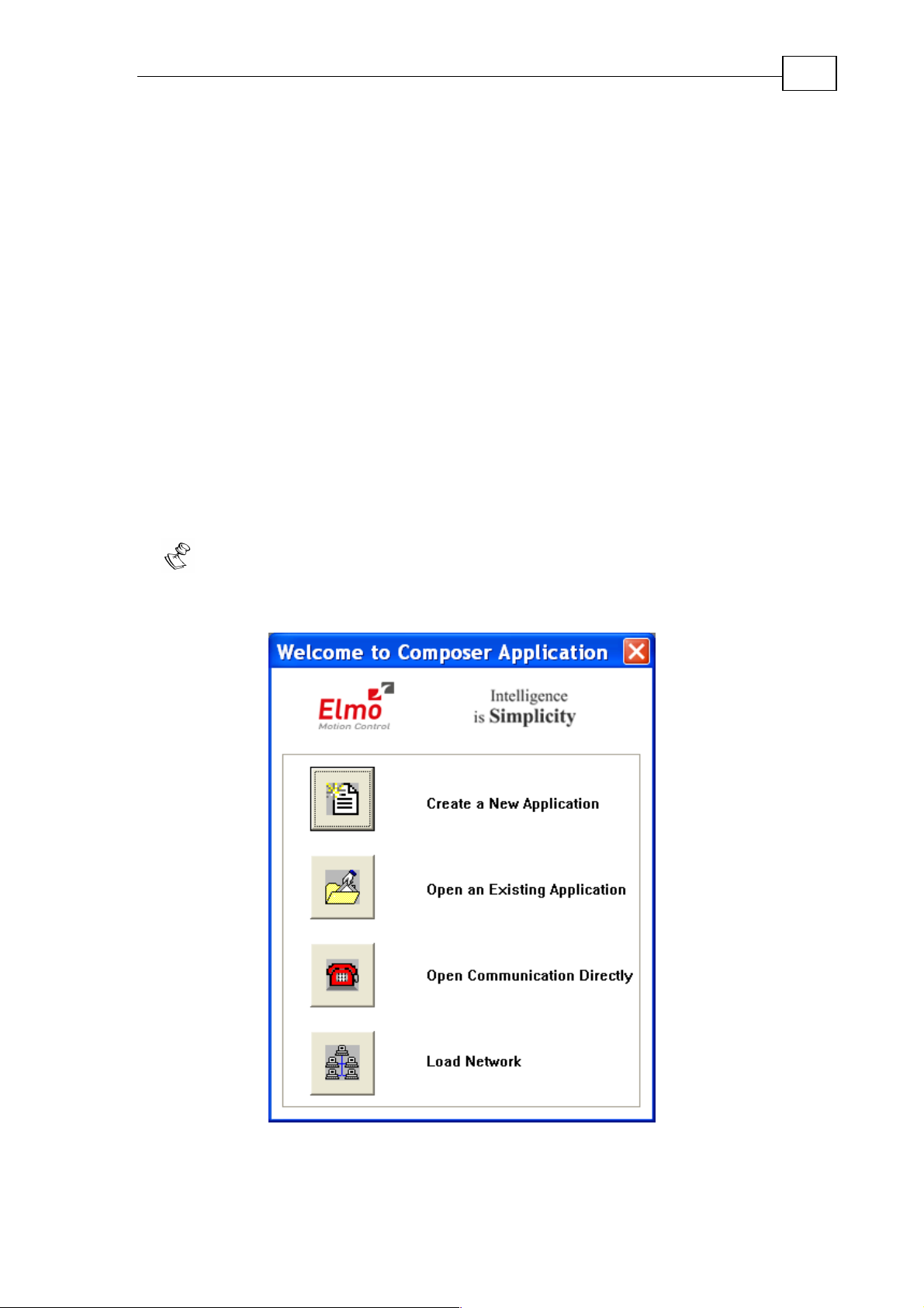
When you open the Composer, the following window opens:
Figure 1: Starting the Composer
Click Open Communication Directly. The following window opens:
Page 9
The SimplIQ for Steppers Getting Started & Tuning and Commissi oning Guide
MAN-BELGS (Ver. 1.1)
9
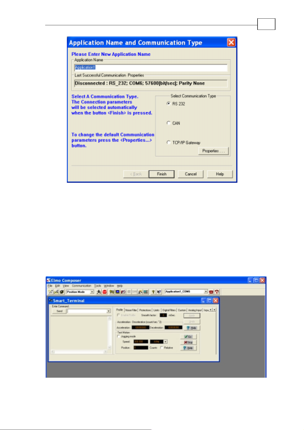
Figure 2: Composer connecting window
Ignore the Application Name field.
Look at Last Successful Communication Properties. If the properties listed there
are as required, click Finish. Otherwise, click Properties:
For RS-232 you need to set the number of the COM port in use, the baud rate
and the parity. The communication is always 8 bits in a byte, and it has one stop
bit.
For CAN you need to set the ID and the baud rate. In addition, you will have to
select the CAN adapter from the supported types.
Then click Finish. The Composer opens to the main window:
Figure 3: The main Composer window
Page 10
The SimplIQ for Steppers Getting Started & Tuning and Commissi oning Guide
MAN-BELGS (Ver. 1.1)
The Smart Terminal lets you enter commands manually – please refer to the
SimplIQ for Steppers Command Reference Manual. To send a command, type it
in the Enter Command field and click Send.
Notes:
At the connection step you need to know the drive communication param eters.
It is possible to change the drive communication parameters only later, after
communication is established.
If you do not know the CAN ID, you may either:
o Connect first with RS-232, then ask for PP[13] (can ID) and PP[14] (CAN
baud rate).
o Use the DSP 305 protocol to find out the drive parameters (you will need
your own CAN application for that).
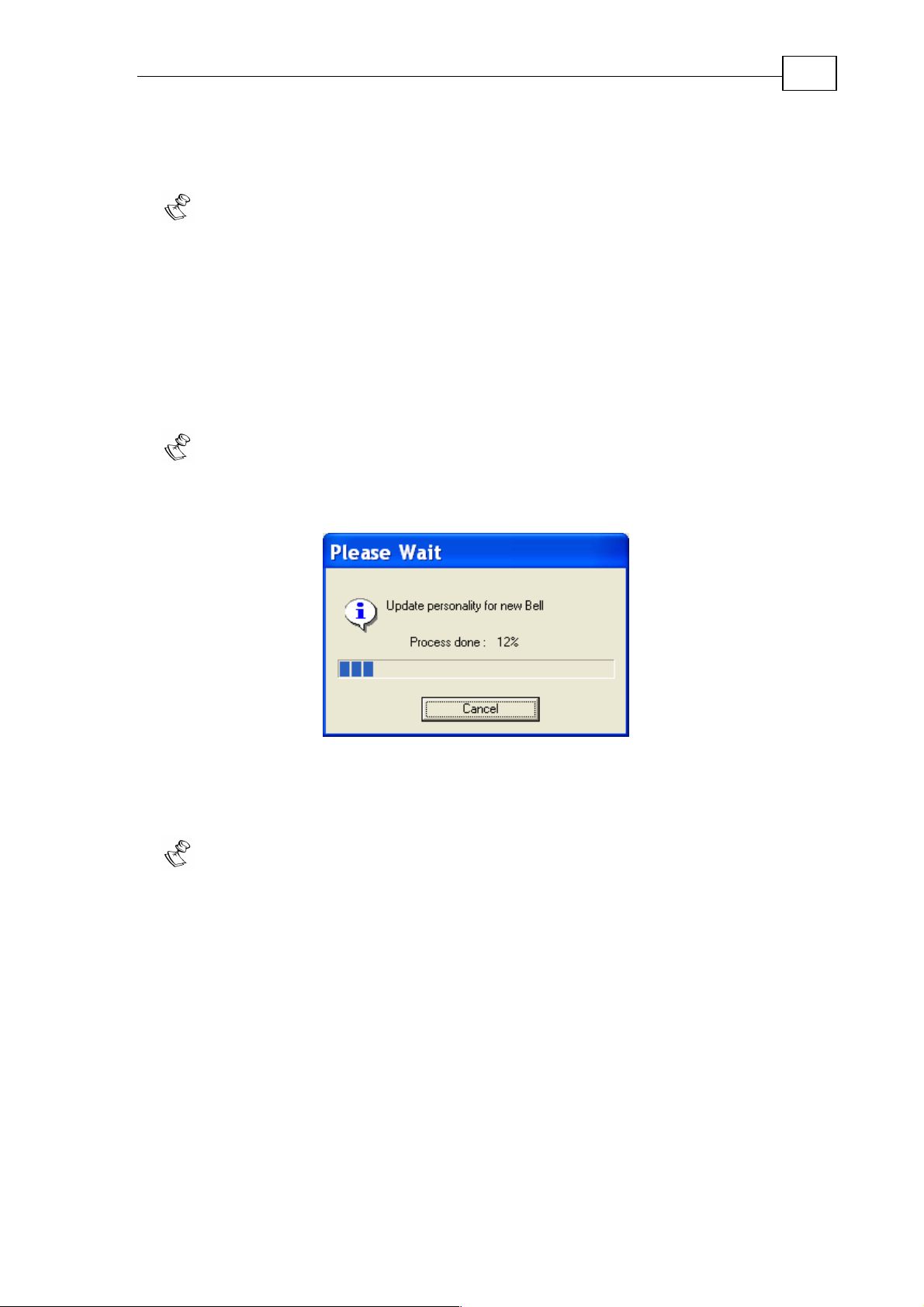
The drive stores a lot of information about itself internally and this enables
the Composer to interact with a multitude of drive types. When a Composer first
meets a drive version it uploads this internal information. You will see the
following window:
10
Figure 4: Uploading personality data
The next time you contact the same drive version, the Composer already has all
its personality data stored and will not ask you to wait again.
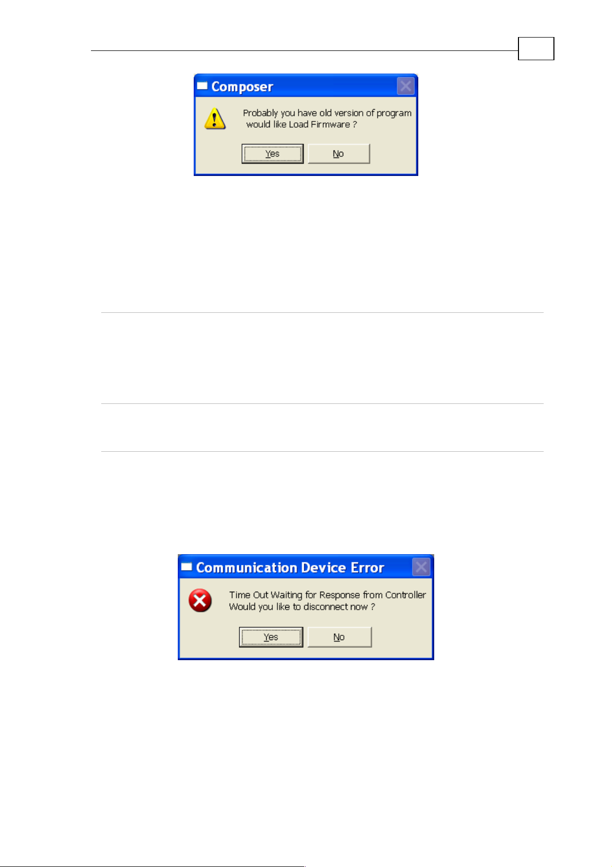
If the drive lost its software, for example by a power-down during firmware
downloading, it will withdraw to a very limited default, or "boot" software. With
this boot, it is only possible to download the new firmware version. The
communication parameters in the "boot" state are fixed (not affected by any user
setting):
Baud rate of 57600 and no parity for RS-232.
Baud rate of 500000 and CAN ID of 127 for CAN.
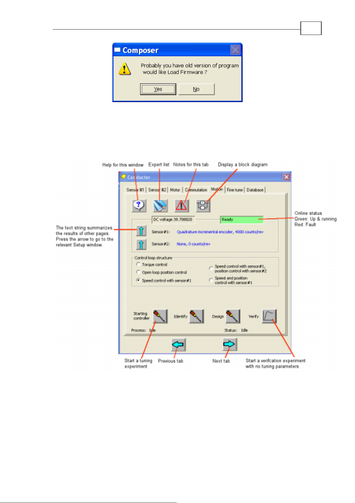
After you set the correct communication parameters, you will see the following
message:
Page 11
The SimplIQ for Steppers Getting Started & Tuning and Commissi oning Guide
MAN-BELGS (Ver. 1.1)
Figure 5: Boot software message
Click Yes to open the windows related to downloading the firmware.
2.1.1 Changing the Communication Parameters
2.1.1.1 Changing the RS-232 Communication Rate and
Parity
First set the desired parameters in the Composer smart terminal:
11
PP[2] RS-232 baud rate.
5: 115,200;
4: 57,600
3: 38,400
2: 19,200
1: 9,600
0: 4,800
PP[4] RS-232 parity. 0: None
1: Even
2: Odd
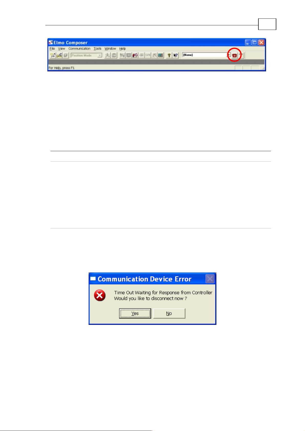
Setting PP[2] and PP[4] alone does not change the communication setting, so the
Composer can continue communication with the drive.
Write, for example, PP[2]=5. This is a requirement for a baud rate of 115200/sec.
Next write PP[2]=1. This is a command to accept the new setting. Almost
immediately, you will see:
Figure 6: Communication disconnect message
This is because you changed the baud rate so the communications from the
Composer fail. Click Yes to disconnect, than re-open communication by clicking
Connect.
Page 12
The SimplIQ for Steppers Getting Started & Tuning and Commissi oning Guide
MAN-BELGS (Ver. 1.1)
Figure 7: The Connect button, circled in red
Next select the new baud rate using the Properties button (See Figure 2).
When the Composer Smart Terminal re-opens, you may use the SV command to
make the new baud setting permanent.
2.1.1.2 Changing the CAN Communication Rate and ID
First set the desired parameters in the Composer smart terminal:
Parameter Description Range
PP[13] CANopen device ID. 1 – 127
12
PP[14] CAN baud rate. 0: 1,000,000
1: 500,000
2: 250,000
3: 125,000
4: 100,000
5: 50,000
6: 50,000
7: 50,000
8: 800,000
Setting PP[13] and PP[14] alone does not change the communication setting, so
the Composer can continue communication with the drive.
Write, for example, PP[13]=5. This is a requirement for the node ID of 5. Next write
PP[2]=1. This is a command to accept the new setting. Almost immediately, you will
see:
Figure 8: Communication disconnect message
This is because you changed the baud rate so the communications from the
Composer fail. Click Yes to disconnect, than re-open communication by clicking
Connect.
Page 13

The SimplIQ for Steppers Getting Started & Tuning and Commissi oning Guide
MAN-BELGS (Ver. 1.1)
Figure 9: The Connect button, circled in red
Next select the new baud-rate using the Properties button (see Fi gure 2).
When the Composer Smart Terminal re-opens, you may use the SV command to
make the new baud setting permanent.
2.2 Application Parameters and Programming
When you commission a drive, you create an Application. An Application refers
to the entire data set you download and store into the drive. The application
includes:
Parameters to store permanently in the drive, such as controller coefficient s.
User programs: please refer to the SimplIQ Programming and Language Guide.
13
The Composer packs all the non-volatile parameters and the User Program in a
single file, with the .dat extension.
The Composer can later use this .dat file to program many amplifiers to the same
parameters and User Program.
2.2.1 Flash, RAM and Tables
The drive contains the following memory types:
Memory Type Used for
Serial Flash Non-volatile This flash stores all the non-volatile
parameters, as well as the User Program
Table Flash Non-Volatile This high speed flash stores the motion
correction tables for real-time use.
The data in the Table Flash must be an
identical copy of the data in the serial flash.
RAM Volatile Stores a volatile copy of the serial-flash
parameters for real-time high-speed use.
When the drive powers-on, it loads the RAM as a copy of the table flash.
It also compares the Table Flash with the Serial Flash. If the contents are not-
equal, you will not be able to start the motor until the situation is corrected.
When you communicate with the drive the parameters you modify are in the
RAM. When you write, for example, KI[1]=1, you update the copy of KI[1] in the
RAM. The parameter KI[1] has a copy in the serial flash which remains as is.
When you want to synchronize the RAM and the serial flash, you can:
Use the SV command to copy the entire RAM contents into the serial flash (for
example, after you tuned some parameters).
Page 14
The SimplIQ for Steppers Getting Started & Tuning and Commissi oning Guide
MAN-BELGS (Ver. 1.1)
Use the LD command to copy the entire Serial Flash contents into the RAM.
When you want to synchronize the Table Flash and the Serial Flash, use the SI=1
command.
Notes:
The SV, LD, and SI commands work on an entire data set. There is no way to
save some of the parameters and not save others.
SV does not automatically synchronize the Tabl e Flash because Tab le Fl ash
synchronizations take a long time. Table Flash synchronizations are carried out
very rarely.
2.2.2 Creating an Application File
In this Section we will create an application file in the PC computer.
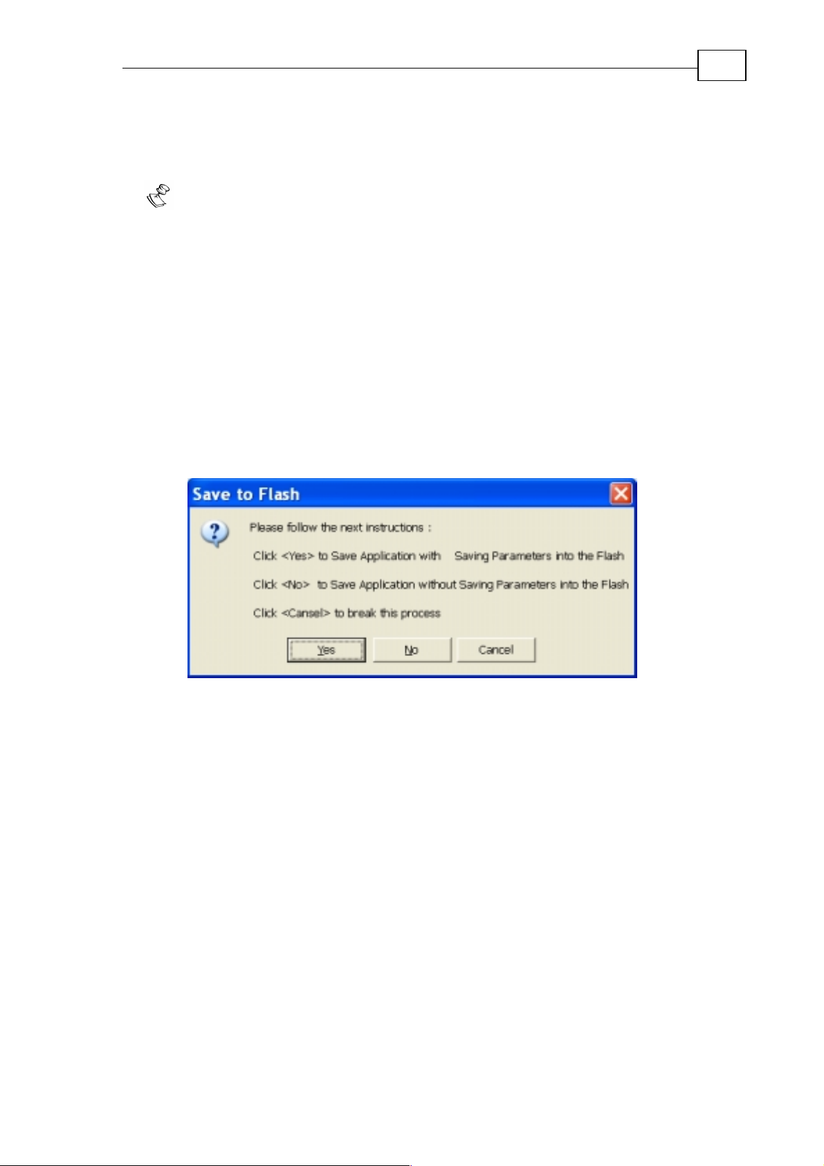
From the menu select File>Save Application.
The Composer will prepare to pack all the parameters and the User Program into
an application file. It displays the following message:
14
Figure 10: Save application message
The Composer uploads the parameters directly from the serial flash. It enables
you to synchronize the parameters in the Serial Flash to the copy in the RAM
<Yes>, or to skip synchronization <No>.
After this enter a file name.
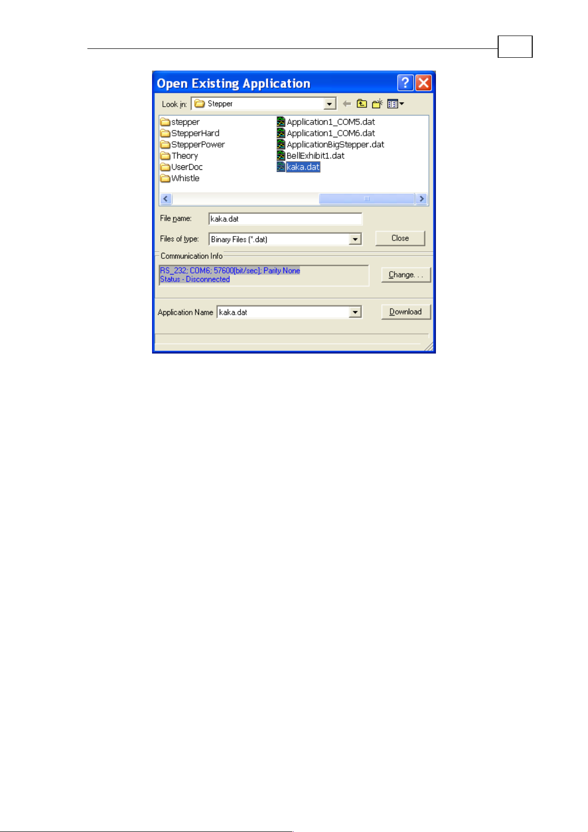
2.2.3 Downloading an Application File
In order to distribute an application from a data file to a driver, do the following:
From the menu select File>Open Application. The following wind ow opens:
Page 15
The SimplIQ for Steppers Getting Started & Tuning and Commissi oning Guide
MAN-BELGS (Ver. 1.1)
15
Figure 11: Open Application window
Upon selection, look at the Communication Info data box. Verify that the
communication parameters there are correct, or click Change to edit them.
Then click Download to complete the downloading.
After downloading, the Serial Flash and the Table Flash may become non-
synchronized, and in this case you need to enter SI=1 at the smart terminal in
order to complete the synchronization.
2.2.4 Observing the Contents and Editing an Application
File
The Composer has a tool called the Application Editor.
2.3 Firmware
This section deals with keeping the drive software version up-to-date.
The drive must be loaded with the correct software to operate. You will normally
receive the drive loaded with the correct software from the dealer. Firmware
upgrades are, however, available from time to time. You can download the latest
firmware from the Elmo web site. It is a text file with the .abs extension.
2.3.1 Version Verification
For version verification, use the VR command. It should return something like
Bell 2.02.07.21 10Dec2007. You can compare this string with the latest available
firmware at the Elmo web site.
Page 16
The SimplIQ for Steppers Getting Started & Tuning and Commissi oning Guide
MAN-BELGS (Ver. 1.1)
2.3.2 Normal Firmware Download
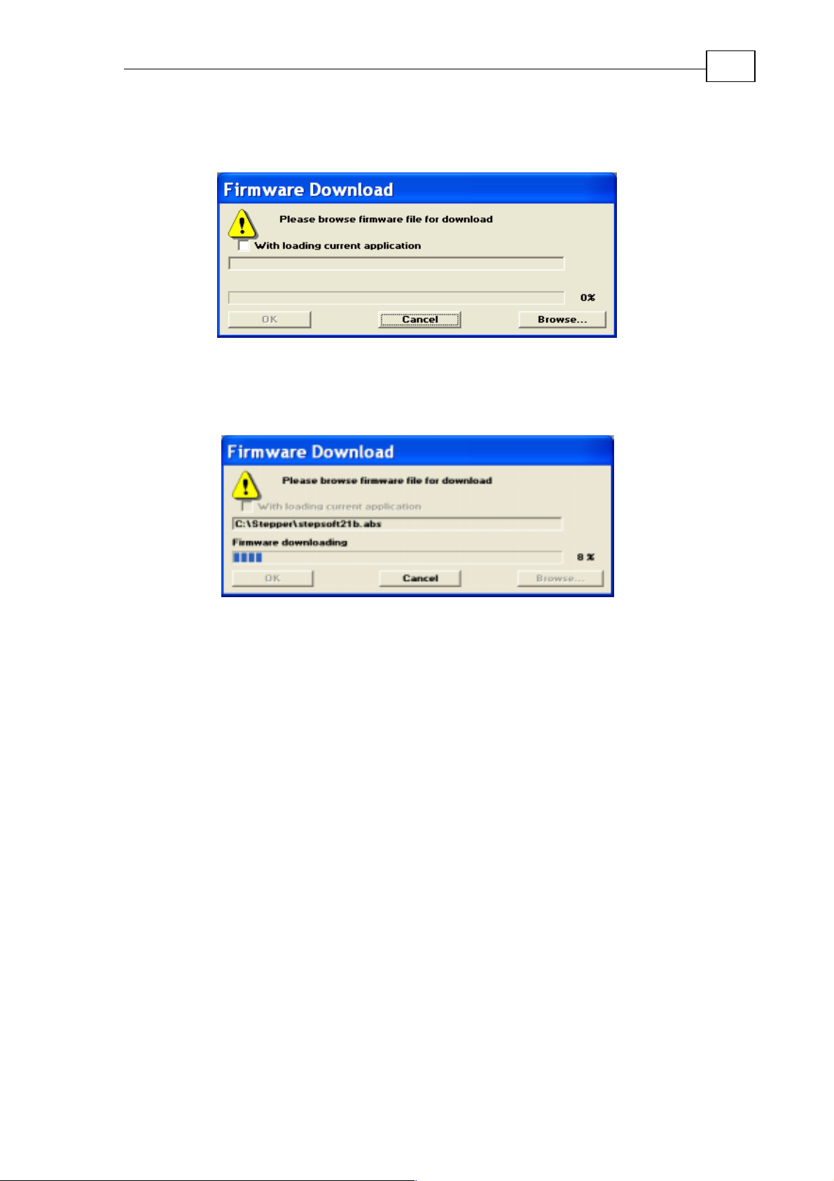
In the Composer Smart Terminal, select Tools>Firmware Download. The
following window opens:
Figure 12: Download firmware window
Use the Browse button to select the firmware .abs file, and then click OK.
The firmware starts to load, and you can watch the progress bar:
16
Figure 13: The Firmware progress bar
The firmware is internally divided into a few sections, and you can observe the
part that is currently being loaded. The first part is "Firmware downloading" and
the last part is "Extended firmware downloading".
When it has finished loading, a message asks you to reboot the drive by
disconnecting it from the electricity.
2.3.3 Abnormal (from Boot) Firmware Download
If the drive lost its software, for example by a power-down during firmware
downloading, it will withdraw to a very limited default, or "boot" software. With
this boot, it is only possible to download the new firmware version. The
communication parameters in the "boot" state are fixed (not affected by any user
setting):
Baud rate of 57600 and no parity for RS-232.
Baud rate of 500000 and CAN ID of 127 for CAN.
After you set the correct communication parameters, you will see the following
message:
Page 17
The SimplIQ for Steppers Getting Started & Tuning and Commissi oning Guide
MAN-BELGS (Ver. 1.1)
Figure 14: Firmware message
2.4 The Conductor Wizard
2.4.1 The Conductor Tabs
The Conductor is the main tool for tuning the SimplIQ control functions.
17
Figure 15: The Conductor window
The Conductor manages some experiments for the tuni ng curr ent and mot ion
controls. You have a lot of flexibility in managing the experiment, but you do not
need to be an expert.
A color code defines which parameter fields you may leave as is, and which require
your attention and understanding – refer to the figure below.
Page 18
The SimplIQ for Steppers Getting Started & Tuning and Commissi oning Guide
MAN-BELGS (Ver. 1.1)
18
Figure 16: User editable fields in a tuning experiment
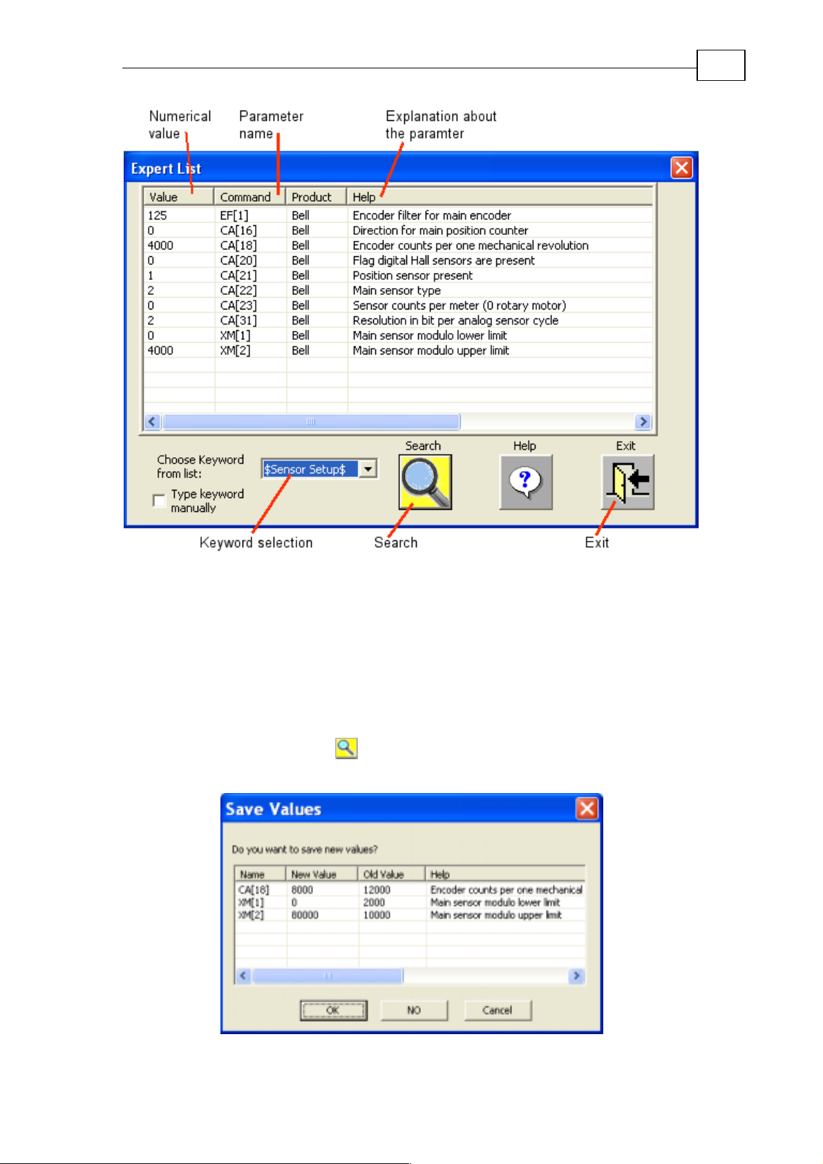
2.4.2 The Expert List
The Expert list is a tool for observing and editing the drive parameters. It gives
extra flexibility for the experienced user, and it lets you track which drive
parameters you changed and how.
Expert lists and the Conductor wizards work with the parameters in RAM
only. Your work is volatile (will disappear at the next power-on or LD
command), until you click Save in Flash in the Database tab.
When you open the Expert List using the Expert list button
following:
, you see the
Page 19
The SimplIQ for Steppers Getting Started & Tuning and Commissi oning Guide
MAN-BELGS (Ver. 1.1)
19
Figure 17: Expert list window
Here you see, and may edit (simply by clicking the value), each of the parameters
that this wizard pad controls.
The Expert List finds which parameters relate to a given Conductor tab using a
keyword; Conductor tabs use keywords that are delimited by $ signs at both
ends.
You can, however, select another keyword from the list, or type a keyword
manually. Then click Search
.
If the Expert List detects a change when you exit, it will display:
Figure 18: Expert List exit comparison
Page 20

The SimplIQ for Steppers Getting Started & Tuning and Commissi oning Guide
MAN-BELGS (Ver. 1.1)
2.4.3 Accepting a Change of Parameters
When you change drive parameters with the Conductor, and you exit a tab, the
conductor displays an exit comparison, as in Figure 18.
After confirmation, the parameters are accepted and cannot be restored by the
Conductor.
Expert lists and the Conductor wizards work with the parameters in RAM only.
Your work is volatile (will disappear at the next power-on or LD command),
until you click Save in Flash in the Database tab.
20
Page 21

The SimplIQ for Steppers Getting Started & Tuning and Commissi oning Guide
MAN-BELGS (Ver. 1.1)
Chapter 3: Getting Started with
Sensors and Motion Control Setup
3.1 Introduction
Tuning a SimplIQ drive to a motor is an ordered, step-by-step process. In this
"Getting Started" chapter, we go through the setup process step by step.
Note that this chapter does not contain all the detailed information for all product
types and cannot take into account every possible aspect of the drive setup.
3.1.1 Tune the Drive to the Motor
All motor and application types:
Set the switch functions for limits; enable functions, brakes, etc. This will create
the initial conditions for the motor to work.
Set the application limits for current, speed, and position. This will prevent
system constraints being violated later on.
21
Defining the sensors.
Selecting the motor type (DC, Stepper, Brushless).
Tuning the current controller.
Brushless motors only:
Commutation tuning (finding how to power the stator so that the motor will
develop maximum torque in the desired direction).
3.1.2 Tune the M otion Control l er
For open loop stepping applications, you only need to set few parameters.
If you have a motion sensor, you may want the following:
Tune speed and position controls.
Set corrections for motor cogging and define the speed-dependent corrections
to the current loop.
3.1.3 Database Maintenance
All the steps until now have manipulated variables in the drive's database. The
last step is to check database validity, and to save the outcome in a permanent
(flash) memory.
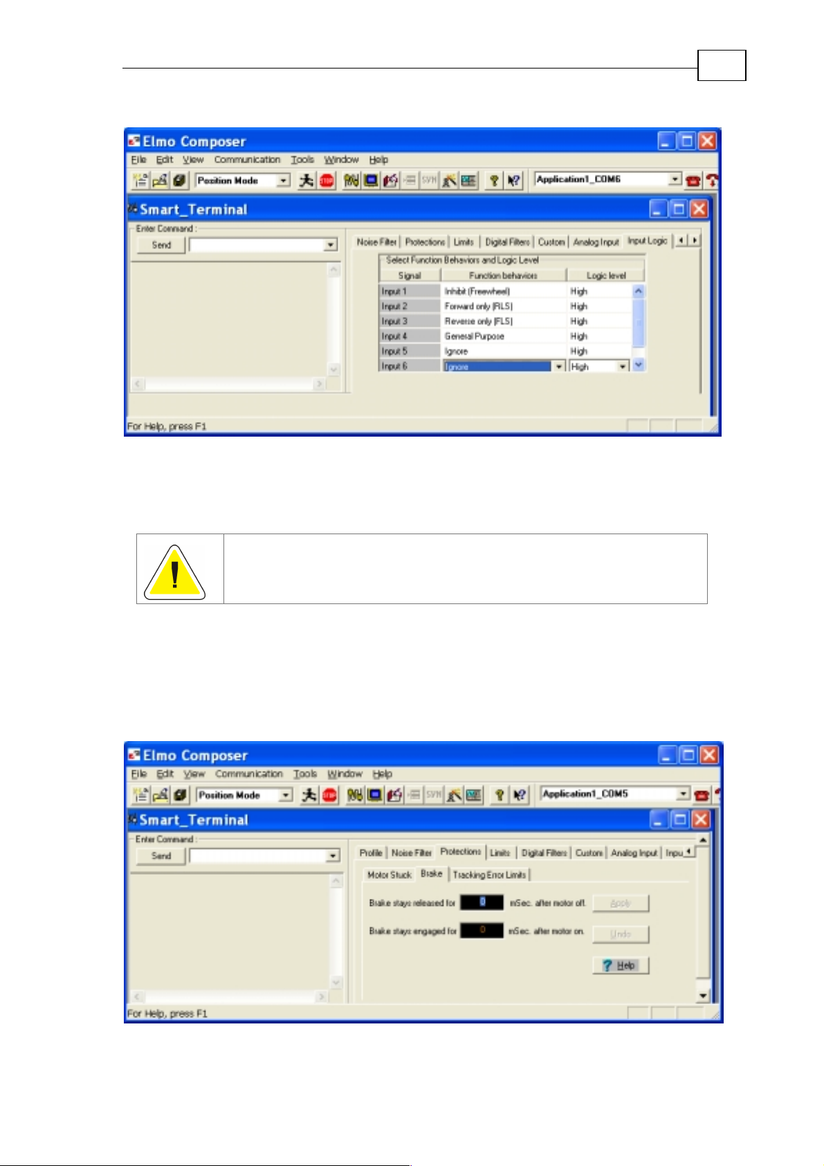
3.2 Abort and Enable Switches
First, set the enabling switches.
The drive has several digital inputs (depending on the drive type). There are
several automatic functions that may be assigned to drive digital inputs.
It is important that at this stage you define which switches are used to abort or to
stop motion, as well as limit switches when applicable.
Page 22
The SimplIQ for Steppers Getting Started & Tuning and Commissi oning Guide
MAN-BELGS (Ver. 1.1)
For this purpose, use the Input Logic tab in the Smart Terminal.
22
Figure 19: Defining input logic
For a detailed description of the functions that may be assigned to digital inputs,
refer to the IL[N] command in the Sim pl IQ for St eppers Com mand Reference
Manual.
Correct digital input definitions help to guarantee that the drive
generates only safe motions in the course of the tuning pr ocess.
Incorrect digital input settings may prevent drive motion or tuning.
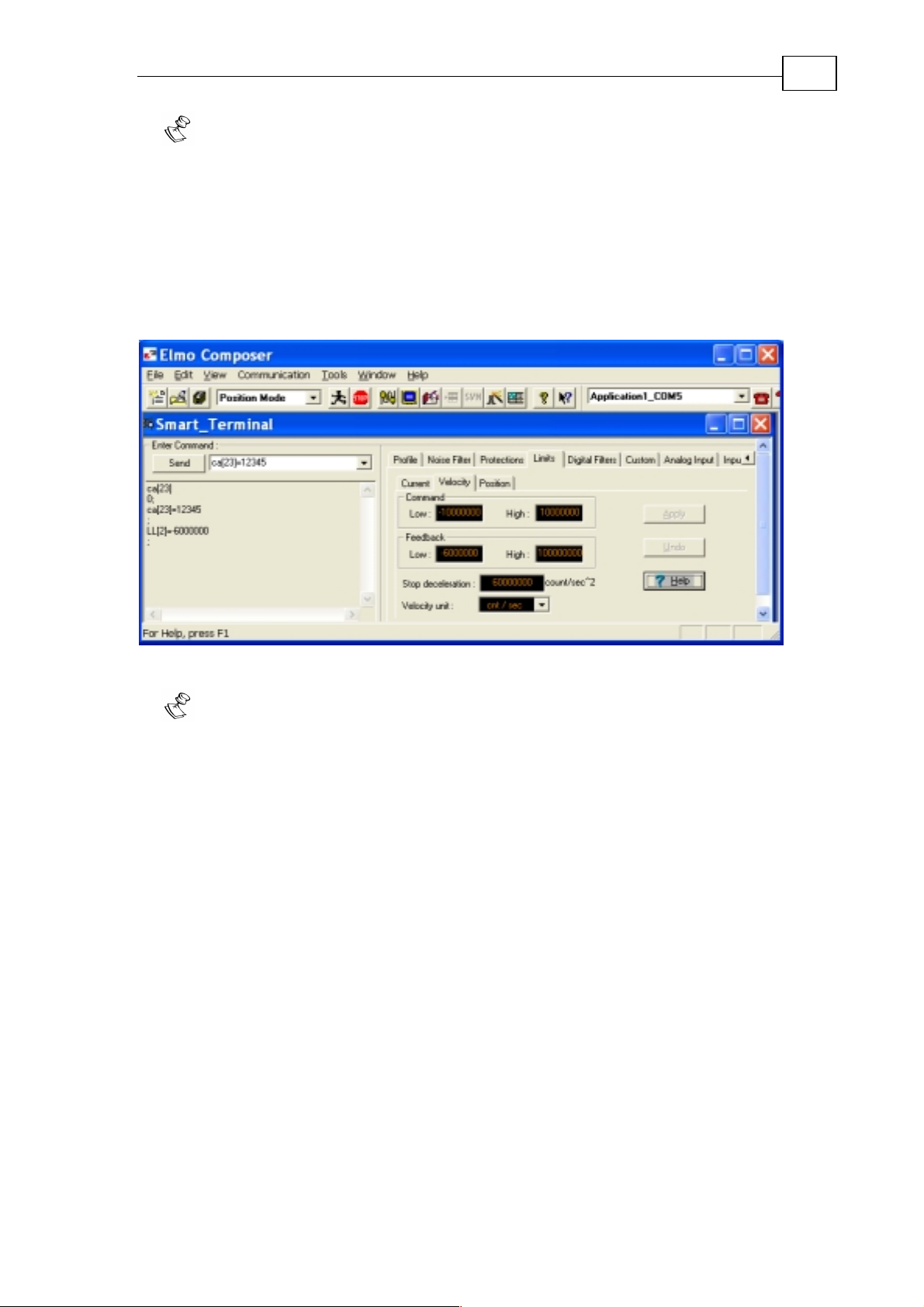
3.2.1 Brakes
If a brake is installed and you want to operate it automatically when the motor
starts, set it up now.
First select the brake engage and release delays. For this purpose select the
Protections>Brake tab in the Composer’s Smart Terminal:
Figure 20: The Brake tab
Page 23

The SimplIQ for Steppers Getting Started & Tuning and Commissi oning Guide
MAN-BELGS (Ver. 1.1)
Do not specify brake delays greater than you actually need.
Next, define the digital output for use as brake control; use the Output Logic tab
of the Composer's Smart Terminal.
For a detailed description of the functions that may be assigned to digital
outputs, refer to the OL[N] command in the SimplIQ for Steppers Command
Reference Manual.
You can test brake operation by programming the brake control temporarily
as a general purpose output, and manipulate it using the OB[N] command.
23
Figure 21: The Output Logic tab
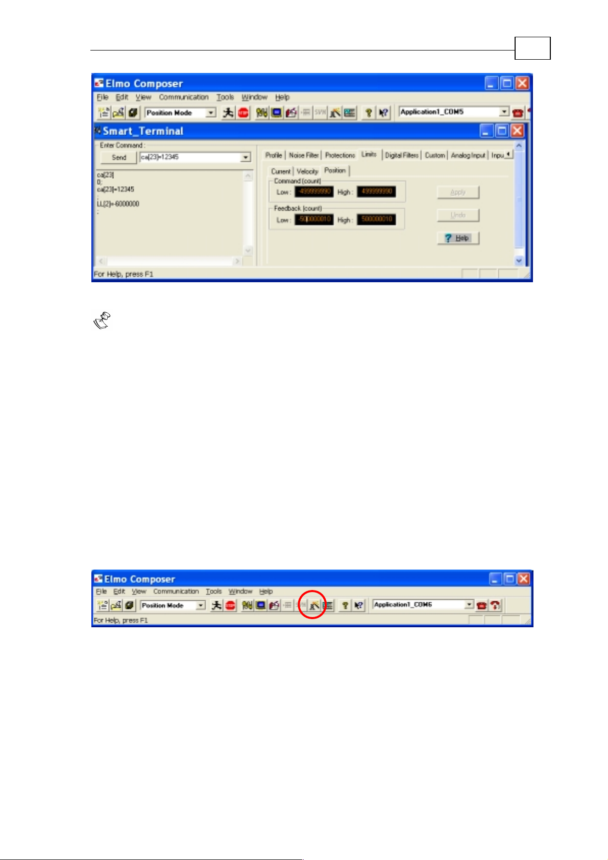
3.2.2 Application Limits
Next, set the application current, speed and position limits. This will h elp to ke ep
the motor within its safe operation range.
Current Limits
Use the Limits>Current tab in the smart terminal:
Figure 22: The Current tab
Page 24
The SimplIQ for Steppers Getting Started & Tuning and Commissi oning Guide
MAN-BELGS (Ver. 1.1)
Notes:
The MC command returns the current limit of the drive peak.
You may set the current limits in the Conductor wizard as well.
Refer to the CL[1],PL[1], and PL[2] commands in t he Sim plI Q for St eppers
Command Reference Manual.
3.2.2.1 Speed Limits
Use the Limits>Velocity tab in the smart terminal:
24
Figure 23: Setting the speed limits
In the Speed Limits tab, you can select RPM as the speed units. For correct
translation between RPM and sensor counts, you need to set the CA[18]
parameter (sensor counts per motor revolution) properly. Take care before you
change CA[18] because if you enter an incorrect value, brushless and stepper
motors cannot work.
3.2.2.2 Position Limits
Open the Protections>Position tab in the smart terminal:
The position command limits apply for open loop stepper applications as well as
for position feedback applications. They do not apply to speed-only or currentonly applications.
Page 25
The SimplIQ for Steppers Getting Started & Tuning and Commissi oning Guide
MAN-BELGS (Ver. 1.1)
Figure 24: Position command limits
Notes:
25
This tab does not set the counting range (modulo limits). You can define the
modulo limits in the setup window of the feedback sensor in the Conductor
Wizard. In an open loop stepping application the relevant modulo limits are
XM[1],XM[2].
The command limits must always be stricter than the feedback limit.
If the command limits are beyond the modulo limits they will be ignored.
3.3 Set up the Sensors
The drive may accept two sensors. Sensor #1 is for speed feedback and possibly
position feedback. The second feedback serves for position feedback, or as a
source for ECAM.
To set up the sensor, open the Conductor tool:
From the Composer, select the Wizard from the tools menu, or use the Wizard
button:
Figure 25: The Wizard button, encircled in red
This will open the Conductor window.
Page 26
The SimplIQ for Steppers Getting Started & Tuning and Commissi oning Guide
MAN-BELGS (Ver. 1.1)
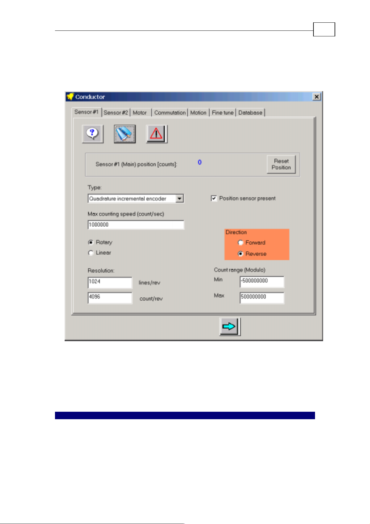
3.3.1 Setting up Sensor #1
Skip this section for open loop stepper applications.
26
Figure 26: Sensor #1 tuning window
Select the type of motion sensor #1.
For a detailed explanation of each of the fields in the tab, click the Help button.
If the motor is small and you can move it by hand, you can observe that the
position readout behaves correctly – either by observing the online position
display, or by taking a record.
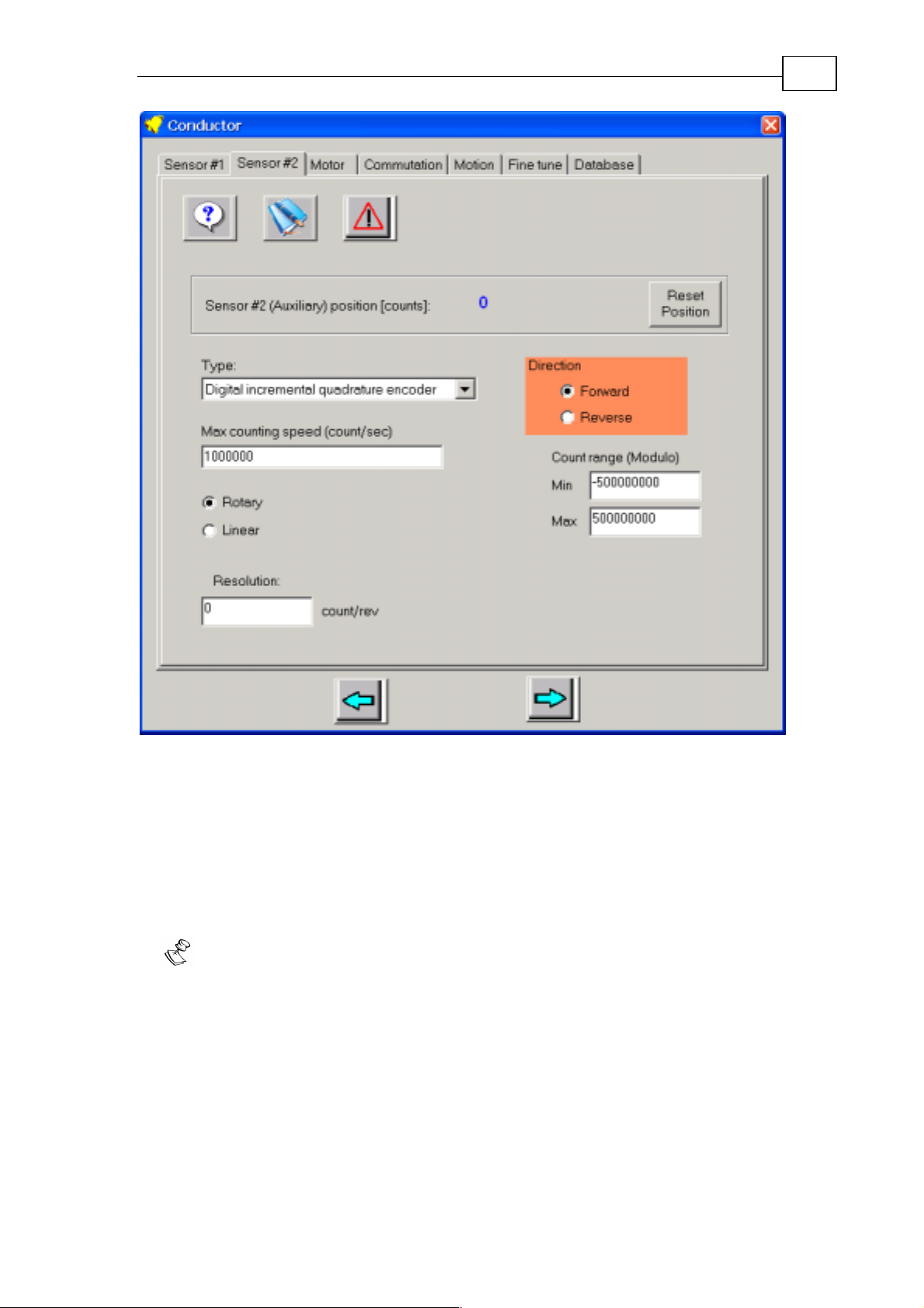
Setting up Sensor #2
You need to set up sensor #2 if you are going to use it for load feedback, ECAM,
or as PWM input.
Page 27
The SimplIQ for Steppers Getting Started & Tuning and Commissi oning Guide
MAN-BELGS (Ver. 1.1)
27
Figure 27: Sensor #2 setup
Sensor #2 can also be configured as a PWM input, or as a PWM output – refer to
the online help.
3.4 Tuning the Drive to the Motor
The next step is to define the motor type. After this step, the digital current
control of the motor will work, at least at the basic level.
The motor tuning will not be complete after this stage. Additional stages are
required, as will be explained, before going to the final fine tuning.
Page 28
The SimplIQ for Steppers Getting Started & Tuning and Commissi oning Guide
MAN-BELGS (Ver. 1.1)
3.4.1 Selecting the Motor Type
The SimplIQ drive can drive DC, 2-phase steppers, or brushless motors.
Notes:
Check that the motor leads are connected correctly. DC motors connect between
M1 and M2. Brushless 3-phase motors connect between M1, M2, and M3, the
phase order does not matter. Steppers connect one phase between M1 and M2,
and the other phase between M3 and M4.
You do not need to know any of the motor parameters (resistance, inductance,
torque sensitivity, etc.) in advance.
You probably do not need to edit the current limiting values, as this was done
at the protections stage.
28
Figure 28: Selecting the motor type
Page 29
The SimplIQ for Steppers Getting Started & Tuning and Commissi oning Guide
MAN-BELGS (Ver. 1.1)
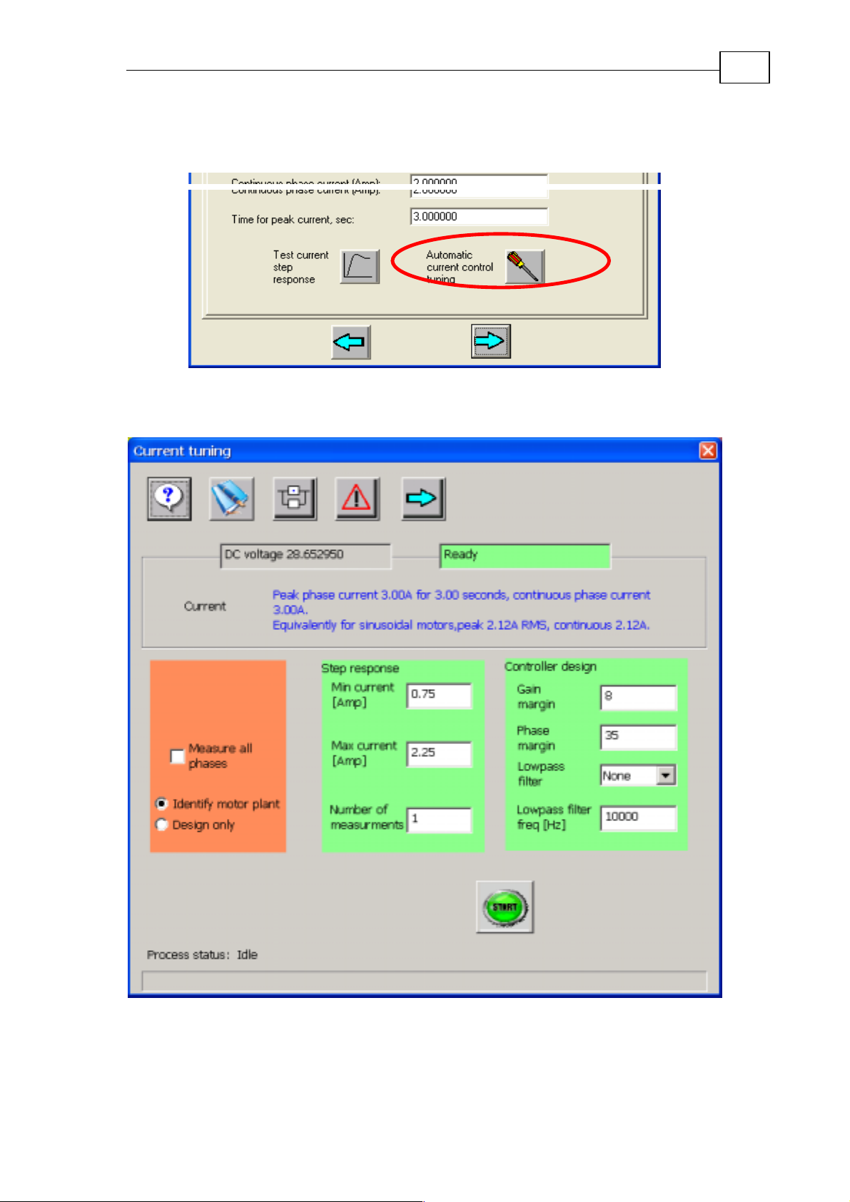
3.4.2 Tuni ng or Checki ng the Current Control
In the same window, select the automatic current control tool.
Figure 29: Entering the current control tuner
The following window opens:
29
Figure 30: Current tuning window
In general, you do not have to change anything in this window, just click Start.
When tuning is over, you will see a graph of the resulting current controller
response.
Page 30

The SimplIQ for Steppers Getting Started & Tuning and Commissi oning Guide
MAN-BELGS (Ver. 1.1)
By clicking the frequency graph button, you can also see the frequency r esponse
of both the open and closed current controller.
Notes:
Setting greater phase margins reduces overshoot , but it also r educes the
bandwidth of the resulting current l oop.
Apply the low-pass filter only if the current control is very noisy (this is very
rare).
Use greater current levels if you suspect the motor is working near magnetic
saturation.
Un-checking Measure all phases will result in shorter, but less accurate current
control tuning.
3.5 Commutation
Commutation tuning means the process of:
Defining which rotation directi on i s positi ve (t his i s a subj ecti ve user decisi on).
30
Learning the order and the polarity at which the motor phases were connected.
Learning the order and the polarity of the Hall sensors (if present).
Adjusting the parameters of the initial rotor position finding – this is essential
for a brushless motor to rotate.
Click the Commutation tab:
Page 31

The SimplIQ for Steppers Getting Started & Tuning and Commissi oning Guide
MAN-BELGS (Ver. 1.1)
31
Figure 31: The Commutation tab
After checking if Digital Hall sensors are installed, go to the tuning process.
The Conductor is responsible to make the motor rotate, so that when the
direction is positive:
The position sensor reading will increase.
The consumed current will be positive.
The problem is that the positive direction is subjective; unless you forced the
sensor direction (to remain as is), the Cond uctor does not know which d ir ecti on
your application calls positive.
To solve this, the Conductor will rotate the motor, and ask you to look at the
motor while it rotates. The following window will open:
Figure 32: Motor direction decision message
Page 32

The SimplIQ for Steppers Getting Started & Tuning and Commissi oning Guide
MAN-BELGS (Ver. 1.1)
Check Reset Commutation Every Hall Edge if your position sensor is not
mounted directly on the motor, but through a gear train or a backlash.
3.6 Motion Tuning
This step depends upon the drive method you choose.
3.6.1 Torque Drive
If you want to enhance the torque control smoothness and performance, you may
want cogging and speed corrections. For that you will need to tune a speed
controller (even though you will disable it later). After tuning the speed
controller, go to the Fine Tune tab, finish the fine tuning, and then back to the
Motion tab to select Torque control.
If you do not need to enhance the torque control, go to the Database tab and save
your work. Then exit the Conductor.
32
Figure 33: Motion tab for torque drives
Page 33

The SimplIQ for Steppers Getting Started & Tuning and Commissi oning Guide
MAN-BELGS (Ver. 1.1)
3.6.2 Stepper Drives with no Commutation Sensor
For stepper drives, click the Motion tab and select either Open loop stepper or
Closed loop stepper with sensor #1.
33
Figure 34: Motion tab
Here you need to enter the holding torque component (static torque, speed
dependent torque, and accelerating torque).
The Motor Calculator button helps you to find the required parameters.
Page 34

The SimplIQ for Steppers Getting Started & Tuning and Commissi oning Guide
MAN-BELGS (Ver. 1.1)
Motor calculator tool
34
Figure 35: Motion tab for stepper
After opening the Motor Calculator tool the following window appears:
Page 35

The SimplIQ for Steppers Getting Started & Tuning and Commissi oning Guide
MAN-BELGS (Ver. 1.1)
35
Figure 36: Motor calculation window
Complete the Inputs section of the form from the motor datasheet; then click
Calculate. This will give the holding torque fixed, speed dependent, and
acceleration dependent components, and also the maximum deceleration SD – f or
further explanations click the Help butt on.
For closed loop position control, this calculator also obtains the dynamic torque
limit PF[29].
You can download the calculated parameters to the drive by clicking Download.
3.6.3 Speed and Position Control
This section describes the speed and position control loop closure wide vi ew. The
details are also described.
There are three options that lead to approximately the same setup actions:
Speed control with sensor #1.
Position and speed control with sensor #1.
Speed control on sensor #1 and position control with sensor #2.
Select one and the Motion tab appears as follows:
Page 36

The SimplIQ for Steppers Getting Started & Tuning and Commissi oning Guide
MAN-BELGS (Ver. 1.1)
36
Figure 37: Motion tab for closed loop control
The Conductor presents an advanced set of motion tuning tools.
The usage level for the tools can be anything from novice to control expert.
Before using the Motion tab read the following sections.
The process is divided into several st eps:
Prepare for identification.
Identification.
Design.
Verification.
This division is because the process may be iterative in which case you may need
to repeat some of the steps.
Page 37

The SimplIQ for Steppers Getting Started & Tuning and Commissi oning Guide
MAN-BELGS (Ver. 1.1)
Notes:
This step assumes that you have properly set the current control and the
commutation in advance. If the current control or commutation are not
optimum, the controller tuning will yield poor results.
If you use analog sensors (Analog encoder, Resolver, Potentiometer, LVDT, etc.)
take extra care to ensure your position signals are clean be fore you s tart motion.
The sensor quality must be tested with the motor fully powered, since RFI from
the motor occasionally disturbs the sensor quality. To find the sensor quality,
open the Composer, set UM=3 (Open loop), set HT[1]=CL[1] (maximum
holding torque), and record the motion sensor Position and Speed. (The
disturbance display on the speed record is much clearer than on the position
record).
3.6.3.1 Prepare for Identification
The control tuning environment needs a working closed loop to start from. The
initial closed loop does not need high performance.
37
Allow the Conductor to find a controller automatically. The Conductor tries to
follow the guidelines of the Appendix on manual tuning automatically. It concludes
with a controller that has quite low performance – only enough to continue
automatic tuning from here.
On starting the Controller tool, the following window opens:
Page 38

The SimplIQ for Steppers Getting Started & Tuning and Commissi oning Guide
MAN-BELGS (Ver. 1.1)
38
Figure 38: Start step designer window
Click Start and wait for the Conductor. Usually it succeeds and you have
completed the process.
If it failed, use the controls and read the online help in order to obtain a working
starting controller.
The starting controller replaces the motion controller with a lowperformance fixed controller. If you had a good controller in the drive before
starting the process of finding a controller, save your work (using the Database
tab) before opening this window.
3.6.3.2 Identification
Identification is the process of finding the transfer function of the controlled
plant. The transfer function will serve you later when you design a controller to
match it.
Page 39

The SimplIQ for Steppers Getting Started & Tuning and Commissi oning Guide
MAN-BELGS (Ver. 1.1)
The method for finding the transfer function is simple: inject sine signals of
varying frequency to the plant and measure the resulting motion. The
implementation of this method by the Conductor, however, is quite complex.
The transfer function of motion systems depends on the signal amplitude and the
working conditions. You can log differi ng tr ansfer funct ions, i denti fied wit h
different working conditions, an d then us e the m all in a co mbine d design proces s
to generate a controller that fits them all.
For quick identification, select the Identify tool.
The following window opens:
39
Figure 39: Identification window
Click Run, answer Yes to confirm the change of control parameters, and wait
until completion. The noises you hear are the frequencies that run through your
plant.
You will receive an identification result with a frequency response plot:
Page 40

The SimplIQ for Steppers Getting Started & Tuning and Commissi oning Guide
MAN-BELGS (Ver. 1.1)
40
Figure 40: Example of a frequency response
Click OK to return to the main identification screen, then save your work using
the File>Save menu. Name it MyFirstIden.idn.
3.6.3.3 Design
With the identification results you can design a controller. The controller has to
meet the following goals:
The robustness figures of merit: acceptable gain and phase margins.
Maximize crossover frequency and low frequency gain for agile and accurate
control.
Minimize high frequency response, in order to attenuate noises and in order to
de-sensitize the controller to the large uncertainti es of high frequency
identification.
These is a conflict between these goals so there is a trade off.
environment of the conductor is built to optimize this trade off.
Example: a completely automatic design: Select the Design tool.
The design
Select the Plant tab and click Add. Select MyFirstIden.idn as the identification
file. The following window opens:
Page 41

The SimplIQ for Steppers Getting Started & Tuning and Commissi oning Guide
MAN-BELGS (Ver. 1.1)
41
Figure 41: Add identified plant to the designer
Select Tools>Automatic design.
The following window opens:
Page 42

The SimplIQ for Steppers Getting Started & Tuning and Commissi oning Guide
MAN-BELGS (Ver. 1.1)
42
Figure 42: Automatic design window
Click Run. The results appear in the following window:
Figure 43: Complete design
Page 43

The SimplIQ for Steppers Getting Started & Tuning and Commissi oning Guide
MAN-BELGS (Ver. 1.1)
You have now completed your first successful design. You can save it to a file.
Select Tools>Download Design, and in the following window:
select the “Position” unit mode.
3.6.3.4 Verification
43
In the verification stage simpl y run st ep responses and j udge t hem accor di ng to
your needs.
Click the Verification tool.
The following window opens:
Page 44

The SimplIQ for Steppers Getting Started & Tuning and Commissi oning Guide
MAN-BELGS (Ver. 1.1)
44
Figure 44: Verification window
Click Start, and the results appear in the following window:
Page 45

The SimplIQ for Steppers Getting Started & Tuning and Commissi oning Guide
MAN-BELGS (Ver. 1.1)
45
Figure 45: Controller verification results
3.7 Fine Tuning
The Fine Tuning tab enables special enhancements to be t uned. Thi s is not
required for all applications.
The following fine tunings are availab le:
Cogging compensation Analog encoder index tuning
3.7.1 Cogging Compensation
The first compensation is for cogging. It becomes availab le when you check
Enable Cogging Compensation.
The cogging compensation adds a compensation torque
motor’s electrical angle; The aim of this window is to map
This mapping can be saved in the drive, saved to a file, or retrieved from a file.
)(T θ where θ is the
)(T θ .
Page 46

The SimplIQ for Steppers Getting Started & Tuning and Commissi oning Guide
MAN-BELGS (Ver. 1.1)
46
Figure 46: The Fine Tuning Tab
On opening the cogging compensation tool, the following window opens:
Page 47

The SimplIQ for Steppers Getting Started & Tuning and Commissi oning Guide
MAN-BELGS (Ver. 1.1)
47
Figure 47: Cogging compensation tuner window
The following options are available:
Set the cogging compensation to default, i.e., there will be no cogging
compensation.
Load a cogging table from a file, without measuring anything.
Measure the actual motor cogging by clicking Start.
When starting a cogging measurement, the following window opens:
When you click Yes, the experiment starts and the progress is displayed at the
bottom of the window.
Page 48

The SimplIQ for Steppers Getting Started & Tuning and Commissi oning Guide
MAN-BELGS (Ver. 1.1)
48
Page 49

The SimplIQ for Steppers Getting Started & Tuning and Commissi oning Guide
MAN-BELGS (Ver. 1.1)
3.7.2 Fine Tuni ng an Anal og Encoder
If sensor #1 is set to "Analog incremental encoder" in the "Sensor #1" window,
then the "Analog index tuning" button i s vi sib le. Thi s tuni ng defi nes the si gnal
level and position where analog index capture occurs.
Please note that for analog encoder, the index appears at different positions for
forward travel and for reverse travel; both cases are measured.
49
Figure 48: The Fine Tuning window whem sensor #1 is an analog encoder
When you click Analog Index Tuning, you need to define the experiment motion
in the following window. The motion has to traverse the analog encoder index.
Page 50

The SimplIQ for Steppers Getting Started & Tuning and Commissi oning Guide
MAN-BELGS (Ver. 1.1)
50
Figure 49: Analog index tuning
After you set the parameters for the experiment, click Start to begin; progress is
displayed in the progress bar at the bottom of the window.
Page 51

The SimplIQ for Steppers Getting Started & Tuning and Commissi oning Guide
MAN-BELGS (Ver. 1.1)
3.8 Database Maintenance
Finally, save the results. Click the Database tab:
51
Figure 50: Database maintenance tab
Check the database integrity. This checks for certain conflicts that can prevent
the motor from starting. For example, if you selected a commutation finding
method by CA[17] that does not match the installed sensors, the motor will not
start and it will report "Bad Database". Checking the database here will prevent
this error.
Save your parameters in flash memory.
Restore your previously stored parameters from flash memory if you want to
purge your Conductor session.
The Expert List of this window brings up the entire SimplIQ database.
Page 52

The SimplIQ for Steppers Getting Started & Tuning and Commissi oning Guide
MAN-BELGS (Ver. 1.1)
Chapter 4: Advanced Control Tuning
This chapter is intended for users wishing to use the extra flexibility of the
motion control tuning system beyond the "getting started" level.
52
This chapter assumes you are familiar with Section
Feedback design is a four-step procedure.
The first step is to generate a low performance controller that is called the
"starting step controller".
This minimal controller only has to stabilize the motor while the plant dynamics
are identified. The Getting Started
Appendix, covers this step.
The second step is to identify the plant model, that is, to find its transfer
function; amplitude-phase versus frequency. Several frequency response
measurements can describe the same plant in order to reflect plant uncertainty.
The third step is to design a controller to match the plant's frequency response.
The user orients the design optimization by emphasizing design margins,
bandwidth, or noise attenuation.
The fourth step is verification – running a 'field' evaluation test.
Notes:
The "Getting Started" chapter has taken you through all these stages, choosing
full automation. This chapter goes over the tuner options in greater detail.
chapter, together with the Manual Tuning
3.6.3.
The feedback design process may be iterative – you can return to the design
stage to improve on the test results, or you can return to the identification stage
to add the results of new working points.
The auto-tuner is very flexible regarding these steps, as explained in the
following sections.
4.1 Start Step Control
4.2 Identification
This chapter deals with identifying the plant including, its uncertainty.
Notes:
This Chapter focuses on understanding what you do rather than on detailed
explanations of the window controls.
Detailed explanations of the window controls are in the online help.
The window controls may differ between Conductor versions, so the
explanations given here may also vary slightly.
Page 53

The SimplIQ for Steppers Getting Started & Tuning and Commissi oning Guide
MAN-BELGS (Ver. 1.1)
4.2.1 Identification and Uncertainty
The identification produces a frequency response. A frequency response is a
characteristic of a linear, time invariant plant. We take frequency response not
because the plant is really linear and time invariant; but because all the
established control design theory d eals wi th pl ants havi ng frequency r esponses.
Knowing very well the limitations of frequency responses, the DFT tuner
identifies many frequency responses instead of one. Each frequency response
describes the plant linearized about a different working point.
After this process, you will have many measured values for th e amplitu de/ph ase
of the plant at any given frequency. This set of values forms an "uncertainty set"
for the frequency.
Later, the Conductor will design a controller that optimizes the response to the
entire uncertainty set. This is much better than traditional methods that can only
consider one plant model at a time.
53
When the Conductor presents the identification result it normally shows one
nominal transfer function. This is because handling a multitude of transfer
functions is very complex.
Identification is an involved process, as it is nonlinear and noisy.
The Conductor is based on many years of trials and collecting data from actual
motion systems.
4.2.2 Identification Results Management
The Conductor stores the identification results in files with the .idn extension.
An identification file stores a list of frequencies and th e as soc iated amplitude an d
phase values of the plant transfer function.
You can keep several .idn files, each describing the plant with different working
conditions.
Identification file maintenance is from the window that opens by clicking
Identify in the Motion tab of the Conductor.
Page 54

The SimplIQ for Steppers Getting Started & Tuning and Commissi oning Guide
n
MAN-BELGS (Ver. 1.1)
Ope
Sav e
New
Cleanu p
54
Figure 51: Identification file maintenance options
You can reset the identification pr ocess (New) and stor e resul ts (Sav e).
You can also edit existing identification results.
You can add frequency points to an existing identification. Open an existing
file, then add the frequencies you want (further details appear later in this
manual). This means that if you want to add data in a certain frequency region
you do not need to go through the entire identification process.
You can clean outliers from frequency responses (Cleanup) – deleti ng an
identified frequency which you consider unreliabl e
4.2.3 Identification Work Point
Identification is the art of exciting the plant with signals, so that its response will
reveal the most about its nature.
The Conductor identifies frequency responses, thus it naturally selects sinusoidal
excitation. Applying pure sinusoidal excitation in an open loop may not be such
a good idea – the motor may drift away and high frequency data may be
completely obscured by frictions.
The Conductor uses the "Starting Step" controller to set the plant working point;
at this working point it applies the sinusoidal exciting signals.
You need to help the Conductor in selecting the identification work-point, from
the following options:
Stay in place: The start step controllers hold the motor more or less in a fixed
position. The motor will hardly drift; the identification will suffer from
frictions.
Page 55

The SimplIQ for Steppers Getting Started & Tuning and Commissi oning Guide
MAN-BELGS (Ver. 1.1)
Free: For non-restricted displacement around the initial position. The starting
step controller will keep the motor w ith con stan t sp eed, s o th at the friction s w ill
minimally affect identification. This mode gives the best linear identification.
Bounded: For restricted displacement around the initial position with given
position limits around the initial position. This mode gives most of the Free
mode advantages when you cannot allow free rotation of the motor.
You can identify in each of the "Stay in place", "Free" or "B ounded" modes.
The comparison will inform you how frictions affect your system; and the later
control design may consider all the cases.
The following figure shows your selection. The window opens by clicking
Identify in the Motion tab of the Conductor.
55
Figure 52: Selecting the identification method
Check Identify Aux. Sensor if you intend to use sensor #2 for position control.
4.2.4 Selecting the Identification Frequencies
The Conductor applies sine signals to the plant . Each si ne signal must be
maintained long enough for the transients to disappear, then the Conductor can
extract the frequency response for that single frequency.
Putting so much energy in a single frequency gives the best results which are also
the most noise immune. However, the identifi cation i s slow.
The Conductor must select the identification frequency with care, so that:
It will find all the critical plant data, without missing important points.
It can complete the identification in a reasonable time.
The Conductor applies an iterative search which first spans a broad set of
frequencies.
Where it finds large amplitude or phase gradients, it applies denser frequencies.
Where the frequency response looks locally smooth, it accept s it .
Page 56

The SimplIQ for Steppers Getting Started & Tuning and Commissi oning Guide
MAN-BELGS (Ver. 1.1)
Although the automated frequency search works well in m ost cases, t he
Conductor may miss very narrow resonance/anti-resonance pairs.
We recommend that you first let the Conductor identify with automated
frequency search.
Check Automatic Refinement to allow intensified resolution where the
frequency response changes rapidly, e.g. near resonant modes.
Make manual adjustments when:
The identification results do not look continuous and smooth enough.
You suspect, based on the evaluation results, t hat the Cond uctor m issed a
resonance.
For this purpose, use the Frequency Editor.
56
Figure 53: Selecting the frequency editor
If you open the Frequency Editor before you have an identification result, the
window looks like this:
Page 57

The SimplIQ for Steppers Getting Started & Tuning and Commissi oning Guide
MAN-BELGS (Ver. 1.1)
57
Figure 54: Frequency Editor, when no identification is available
The red points, and the list in the Frequency area, show the frequencies for plant
excitation. For every frequency there is also an associated excitement current
amplitude.
Before the identification you can see the default set of frequencies that the
Conductor sets before learning the plant.
Bigger current amplitudes generate a better signal to noise ratio, and are thus
better for identification. There are other considerations, however:
o Large currents at high frequencies tend to saturate the amplifier voltage
due to motor inductance. This saturation is reflected in the identified
transfer function by decreased amplitude and increased delay.
o Large current near resonant modes lead to unpleasant noises, or even
mechanical damage.
After clicking Run Identification the window appears as follows:
Page 58

The SimplIQ for Steppers Getting Started & Tuning and Commissi oning Guide
MAN-BELGS (Ver. 1.1)
58
Figure 55: Frequency editor window after identification
The blue points show identification results.
There are no red points and no point listing in the selection box since all the
frequency points have been run and there has not yet been a new request.
You can add and edit new frequency points and run them; their identification
result will be appended to the existing frequency response results.
For the above identification, the resolution seems poor near t he anti resonance
and near the 2-3-4 resonances. We would like to increase the resolution there, and
use the Add>Graphics tool.
Add the red frequency points to the graph; on the next "Run Identification" only
the frequencies you added will be identified, and appended to the existing
identification record.
Notes:
Poor resolution usually reflects in the phase window being clearer than in the
amplitude window.
Do not confuse 360
°
phase jumps with phase resolution problems. Phase jumps
of 360° (see the right end of the above phase plot) come from angle display
folding.
Page 59

The SimplIQ for Steppers Getting Started & Tuning and Commissi oning Guide
MAN-BELGS (Ver. 1.1)
59
Figure 56: The Frequency Editor
Page 60

The SimplIQ for Steppers Getting Started & Tuning and Commissi oning Guide
MAN-BELGS (Ver. 1.1)
Appendix A: Manual Tuning of Speed
and Position Control
A.1 Scope
This Appendix explains how to manually tune control ler s of the foll owi ng types:
1. A PI speed controller.
2. Cascaded position controller: The inner loop is a PI speed controller and the outer
loop is a position simple gain controller.
3. A PI speed controller with a single notch filter, a low-pass filter or both.
4. Cascaded position: The inner loop is a PI speed controller with a single notch filter,
a low-pass filter or both; and the outer loop is a simple gain.
The notch filter and/or low-pass filter are termed in this document as "High
order filters".
if the sensors are noisy with systems that exhibi t r esonance, and when i t i s
essential to decrease high frequency motor curr ents. The Hi gh order fil ter can
improve the controller performance dramatically when used correctly. Incorrect
usage of the High order filter can lead to a poor or even unstable controller.
High order filters are expected to improve closed loop performance
60
Use the manual tuning as a starting point for automatic tun ing: Au tomatic tuning
brings better results than human t uning i n most cases.
Notes:
This appendix concentrates on manual tuning tips and theory, and it does not
provide an accurate description of controller parameterization. For that, refer to
the KP[N], KI[N] commands etc in the SimplI Q for Stepper s Comm and
Reference Manual. All the relevant commands have links to the full control
structure description.
This appendix does not describe the tuning interfaces – see the sections on
motion tuning for that.
We strongly recommend familiarizing yourself with the controller structure and
parameterization before attempting to tune it.
A.2 Safety
Servo systems must be treated with car e. In the t uning pr ocess, they must be
treated with extreme care. Although we have made our best efforts to generate
safe tuning conditions:
In the tuning process, the motion controller may become unstable, leading to an
abrupt, unexpected response.
In the tuning process, the motion controller may become very weak, letting
disturbances and external loads drive the shaft.
Read this appendix carefully before launching an experiment, and evaluate the
experiment parameters carefully before launching it. The Conductor suggests
some experiment parameters, but it may mislead you, being unaware of your
specific limitations.
Page 61

The SimplIQ for Steppers Getting Started & Tuning and Commissi oning Guide
MAN-BELGS (Ver. 1.1)
Treat unbalanced1 systems with extreme care.
A.3 Make it Simple
This Appendix gives some simple guidelines for manual controller tuning. In
order to simplify the tuning process we di vi de i t int o a seri es of steps.
The rules of simplification are:
Never tune your controller to perform better than you need. A controller of
lower bandwidth decreases stresses and is m ore ro bust to changes and ageing.
In this Appendix you will learn how the High order filter may decrease control
stresses.
Tuning a speed controller is simpler than tuning a position controller. If you
need to tune a position controller, try to tune first its embedded speed
controller. The Conductor program lets you tune a speed controller without the
risk that the motor will drift away from its starting shaft position.
If your mechanics are simple and good enough to avoid the High order filter,
adhere to the simple PI speed controller. The High order filter requir es more
skill to use. The High order filter always introduces a filtering delay, which
usually limits the achievable bandwidth compared to a simple PI.
61
Use the High order filter when encountering oscillations and high frequency
noise. The small extra effort of tuning the High order filter can b e very
beneficial.
If your encoder has good enough resolution and the friction is low enough, use
a fixed controller.
Use controller scheduling (dynamic adaptation of the controller parameters to
the situation) if you have a low-resolution encoder or high friction. The extra
effort of tuning the High order filter can be very beneficial.
Work linearly. With high controller gains the current command saturates for
very small tracking errors. The saturation makes the evaluation of control
quality very difficult. Keep the motions small enough and verify by the current
waveforms that the current command does not saturate2. Verify how the
controller works with large signals only after it is satisfactory with small
signals.
Work with steps. When you test a controller with limited acceleration or even
smoothed reference waveforms, don't excite high frequencies. The results will
not reveal oscillations and high frequency problems that may exist.
Do not fear overshoots. Overshoots are necessary if the controller is to track
without a time delay. Reducing the height of the overshoots lengthens their
duration. Evaluate the overshoot that you can tolerate by experimenting with
acceleration limited test waveforms, without exceeding the acceleration you
actually use.
1
Systems that do not stay in place when the motor is shut down.
2
Note that the rate of change of the current command is also limited. This is because
dI
max
inductance.
V
B
= where I is the motor current,
dt
L
V is the supply voltage and L is the motor
B
Page 62

The SimplIQ for Steppers Getting Started & Tuning and Commissi oning Guide
MAN-BELGS (Ver. 1.1)
A.4 Keep Margins
It is very tempting to increase the controller gains and enjoy the maximal
performance of your system. You must bear in mind that the price of maximum
performance is decreased robustness to system variations. The higher the gains, the
greater the chance that the system will become noisy or even unstable due to
changing work conditions, or due to ageing. The following tips will help you create
a stable, long-lasting motion system:
Tune for minimum inertia. If the inertia of the system varies, e.g. for a rot ary
robot arm, tune for minimal inertia
higher inertia will have a slower response time, but are likely to remain stable.
The controller must remain stable (it does not have to maintain an optimum
response) when you double the selected gains, and also when the selected gains
are reduced by half4.
Acceleration limits. For a position controller, the maximum motor acceleration
(parameter GS[9]) must be set high enough so that it does not disturb normal
operation, but also low enough so that it prevents position disturbances from
creating large overshoots.
3
. Positions or loading conditions with
62
A.5 The Basic Concepts
This section concisely and informally explains the entities you will come across
when tuning.
A.5.1 Fixed- vs. Gain-scheduled Controllers
The drive can run either a fixed- or a gain-scheduled controller. A fixed controller
runs a fixed set of control parameters
Gain scheduling is the process of adapting the controller parameters "on the fly"
to a given situation. The Drive stores 16 sets of controller parameter sets. The
active controller parameters set is chosen by the gain scheduling process.
The drive supports two types of gain scheduling.
Automatic gain scheduling: the Drive adapts the controller to the speed
controller command, in real-time. The reasons for automatic gain scheduling
are:
o When the speed becomes low, there is a large delay between consecutive
encoder position updates. This delay requires a decreased controller
bandwidth.
o At low speeds friction becomes a dominant control problem. Increasing
the integrator gain at low speeds may improve low speed behavior.
5
.
3
Tuning for the least inertia may have a high price with high inertia postures or load conditions. You
can tune instead for several postures or loads and apply manual gain scheduling.
4
If you tune a speed controller you don't have to test with halved gains. Position controllers are,
however, conditionally stable. This means that a position controller will loose stability with gains that
are small enough.
5
The fixed/scheduled option refers to the proportional and the integral speed gains, position gain, and
some parameters of the Advanced filter.
Page 63

The SimplIQ for Steppers Getting Started & Tuning and Commissi oning Guide
MAN-BELGS (Ver. 1.1)
Manual gain scheduling: The controller parameters may adapt due to a user
program or an external command. For example, the controller gains of a winder
may be increased as it rolls and gains weight.
For convenience, when you program a fixed controller you don't overwrite the
schedulable parameters, and vice versa.
The Auto-tuner always programs an automatically gain-scheduled controller.
A.5.2 Resonance and Notch Filters
Resonance is a very common mech anical ph enome non , in w hich a flex ible s ys tem
vibrates in its natural frequencies. In many applications, the natural frequencies
are too high for the motion controller to control. The best policy for the motion
controller is then to avoid exciting the oscillations. You chain a band-stop (notch)
filter to the controller to prevent the controller from driving the oscillatory
frequency.
If you don't use a notch filter where necessary, either:
Severely limit the possible controller bandwidth.
63
Risk instability and extreme stresses to the controlled system.
Tips:
Normally there is more than one resonance frequency. It may be necessary to
set more than a single notch.
In some systems the resonance frequency changes significantly due t o l oad or
posture changes. Verify that your designed notch covers the entire operational
envelope.
A.5.3 High Frequency Noise and Low-pass Filters
High frequency noise means vibration, acoustically unacceptable noise, and
much greater power consumption than is necessary just to drive the motor to its
desired shaft position. The main reasons for high frequency noises are:
Sensor inaccuracy.
Plays or backlash in the mechanics.
High frequency, unidentified resonance, possibly due to ali asing
The best policy for the motion controller is to avoid exciting the motor at a high
frequency because the system vibrates there or because the feedback is not
reliable. For this purpose chain a low-pass filter to the controller.
6
.
The price of a low-pass filter is an equivalent delay. For a double pole filter with
a damping factor of 0.7, the insertion delay is about 0.23/f, where f is the corner
frequency.
6
We deal with a sampled system. High frequency signals may appear to sampled systems in changed,
low frequencies. For example, if the Drive samples at 300 usec (TS=75), then an oscillation with a
period of 300 usec (3333 Hz) appears to the Drive as a constant value (frequency=0).
Page 64

The SimplIQ for Steppers Getting Started & Tuning and Commissi oning Guide
MAN-BELGS (Ver. 1.1)
A.5.4 Evaluating a Step Response – Rise Time, Settling
Time, and Overshoot.
A step response is the waveform (position or speed) the motor exhibi ts when it s
reference command (position or speed) changes abruptly. Step responses are not
very practical in real-life motoring applications, as the reference commands are
nearly always acceleration limited and many times smoothed.
A step response is, however, good to reveal the detailed dynamic behavior of the
controller. The most popular step-response figures of merit are:
Rise time: The time since the reference has been changed until t he value
(position or speed) covers 90% of the step.
Settling time: The time since the reference has been changed unt il the value
(position or speed) remains permanently within 3% of the step.
Overshoot: The percentage of the deviation to the other side while stabilizing
the step.
These figures of merit are shown in Figure 57.
64
1400
1200
1000
Target
800
600
400
200
Time
0
0.011 0.012 0.046 0.050 0.074
Figure 57: A step response: The rise time is about 0.01, the settling time is 0.074, and the
overshoot is about 30%.
The overshoot level, as well as the ratio between the rise time and the settling time,
reflect the gain and the phase margins
7
. Gain or phase margin results that are too
low may result in a high step response overshoot (more than 40%) followed by an
undershoot and a long settling time. If the ph ase margin is too h igh, the se ttling time
is too long. These properties are depicted in Figure 58 below which is a simulation
of three design examples: One with reasonable margins, one with margins that are
too low and one with phase margins that are too high.
7
The gain margin is the factor in which the controller gain can be increased until loosing stability. The
phase margin is the difference of the open-loop phase from -180 degrees at the point where the open-
Page 65

The SimplIQ for Steppers Getting Started & Tuning and Commissi oning Guide
A
MAN-BELGS (Ver. 1.1)
16000
14000
12000
10000
8000
Acceptable margins: Nice response
cceptable margins: good response
Too low margins: large overshoot and oscillations
6000
Step resp onse
Margins too low: large overshoot and oscillations
Too much margins: long settling time
Margins too high: long settling time
Reference
4000
2000
65
0
0 0.01 0.02 0.03 0.04 0.05 0.06 0.07 0.08
Time (sec.)
Figure 58: Comparison between step responses of acceptable controllers and non-
acceptable controllers. Details on the plot.
A.6 The Example System
Manual tuning is not a true science with closed formulas. It is heuristic, and the
heuristics fit only a (relatively wide) selection of systems. All the explanations in
the rest of this Appendix refer to the two laboratory systems, shown below.
Both the systems have the same motor and ampl ifier :
Characteristic Value
Motor type Brushless, three pole pairs, 4 Amp continuous.
Encoder resolution 4000 counts/rev (1000 lines)
Amplifier Bell 5/100
In system #1, the motor is loaded by a simple inertia. This simple inertia load
enables high bandwidth control. In system #2, the load inertia is coupled to the
motor through flexible coupling. The coupling introduces a mechanical
resonance.
loop gain is 0 db. For further explanation, see the Auto-tuning manual, or any basic textbook in control
theory.
Page 66

The SimplIQ for Steppers Getting Started & Tuning and Commissi oning Guide
MAN-BELGS (Ver. 1.1)
A.7 Testing the Response of a Controller
Manual tuning is an iterative process in which you select parameters for the
controller, and then test them.
A.7.1 Current Limits
Beware that the peak current limit and the continuous current limit of the drive
may differ. If you use excessive current levels in the experiment, the drive may
switch automatically to the continuous limit, and exhibit saturation behavior.
A.7.2 Recording the Experiment Results
The Conductor's Wizard records the results of the tuning experiment. The
recorder is automatically triggered when the motion command (speed or target
position) changes.
The recorder records the reference and the actual speed and position waveforms,
and also the motor's current demand. The current demand is very useful for:
66
Detecting saturation. If the current demand is saturated then the system
reached physical limitations, and you cannot distinguish the small signal
response from the experiment result.
Current command waveforms easily reveal phenomena like friction (current
increases for a while before the motor starts to move), cogging (periodic-inposition torque disturbance), dynamic unbalance (periodic-in-position torque
disturbance, proportional to the squared speed), play ( the ratio be twe en curre nt
and acceleration jumps wildly), resonant limit cycle (constant frequency
sinusoidal disturbance) and much more.
Large high frequency current demands reveal the need for high fr equency
filtering in a more vivid way than position or speed error.
Check that the currents are near the expected values for the accelerations used.
This gives you extra assurance that the system is properly assembled and well
calculated.
You can set the recorder time as long as you want, but for large recording times
you will lose resolution, as the number of the recorded data points is limited.
Notes:
The recorder can export the experiment results to Matlab8 for further analysis.
When decreasing the recorder resolution, you become more susceptible to
aliasing. In other words, high frequency dist urb ances may b e tot all y mi spresented, and they may look as phenomena of a much lower frequency.
8
Popular, excellent technical calculations software by MathWorks.
Page 67

The SimplIQ for Steppers Getting Started & Tuning and Commissi oning Guide
MAN-BELGS (Ver. 1.1)
A.8 Fixed Gain Manual Tuning for a Speed Loop
This section deals with choosing the KI and KP parameters of the PI controller
and the parameters of the High order filter. We first describe how to select the KI
and KP parameters. Then we explain how to add a low-pass filter. Finally we
explain how to decide if a notch filter is needed and how to add it.
A.8.1 Manual Tuning of a PI Controller
We present an iterative process of choosing KI and KP and testing the closed loop
step response. We evaluate the step response in order to iterate the KI and KP
parameters for improved closed loop performance.
1. Start with the very low gains of the PI controller: KI=3 and KP=1 for example,
then set the following step reference command parameters:
(a) Set a long recorder time, as with low gains the response is going to be slow.
Here the Max. Record Time is 0.48 seconds.
(b) Velocity: 12000 counts/second (fits 180 RPM for encoder of 4000 counts per
revolution). This may be too slow a velocity for optimal tuning. We will increase
the reference speed later, when we are more confident of the motor's response.
The steps are:
67
(c) Displacement: Displacement of at least Max. Record Time multiplied by
Velocity (about 5000 in this example), unless it violates the mechanical limits.
The test data is summarized in the following table.
KP KI Velocity +Displ. -Displ. Rec. T. Rec. Res Profile
1 3 12000 5000 -5000 0.48 sec 400 musec off
Let us observe two plots, the measured speed and the motor current. With the
low gains the motor's response is very sluggish, as in Figure 59.
4
x 10
1.5
0.6
-0.3
-1.2
-2.1
C ounts /s ec .
Speed
Reference
-3
0 0.1 0.2 0.3 0.4 0.5
T ime (s e c.)
0
-0.03
-0.06
-0.09
Am pere
-0.12
-0.15
0 0.1 0.2 0.3 0.4 0.5
T ime (s e c.)
Figure 59: First test with low KI and KP
Page 68

The SimplIQ for Steppers Getting Started & Tuning and Commissi oning Guide
MAN-BELGS (Ver. 1.1)
Figure 59 reveals the following:
1. The measured output does not reach the commanded step.
2. Current command is far from saturation, therefore you can increase the
velocity command.
Figure 60 repeats the same test with increased velocity and test duration as given
in the table below. Note that there is a long time duration (from 0.7 to 1.3 sec.)
that the velocity is almost fixed while the current increases, this is a result of high
friction.
KP KI Velocity +Displ. -Displ. Rec. T. Rec. Res Profile
1 3 48000 20000 20000 2.4 sec 2 msec Off
4
x 10
1.5
0.6
-0.3
68
-1.2
-2.1
Counts/sec.
Sp eed
Reference
-3
0 0.1 0.2 0.3 0.4 0.5
Time (sec.)
0.2
0.1
0
-0.1
Am pere
-0.2
-0.3
0 0.5 1 1.5 2 2.5
Time (sec.)
Figure 60: A test with the same controller as the test of Figure 59 with a hi gher ve loci ty
command and a longer recording time (Speed2)
1. Repeat step 1, increasing KI and KP simultaneously by 50% at a time until one
of the following occurs:
The step response exhibits an overshoot of about 20%.
The step response is unacceptable for any reason, for example any sign of
resonant oscillation.
The system exhibits large overshoot and undershoot which is a sign of being
close to instability. In this case decrease KP by at least a factor of 2.0.
The final response is in Figure 61, which includes several tests based on increasing
KI and KP with the values given in the following table
KP KI Velocity +Displ. -Displ. Rec. T. Rec. Res Profile
10,20,30,40
6KPπ
12000 5000 5000 0.48 sec 400 usec Off
Page 69

The SimplIQ for Steppers Getting Started & Tuning and Commissi oning Guide
MAN-BELGS (Ver. 1.1)
4
x 10
1.5
KI=120,KP=40
0.9
0.3
KI=90,KP=30
KI=60,KP=20
KI=30,KP=10
Reference
-0.3
-0.9
Counts/sec.
-1.5
0.1 0.12 0.14 0.16 0.18 0.2
T i me (sec.)
1.5
KI=120,KP=40
1.1
0.7
KI=90,KP=30
KI=60,KP=20
KI=30,KP=10
0.3
Am pere
-0.1
69
-0.5
0.1 0.12 0.14 0.16 0.18 0.2
T i me (sec.)
Figure 61: Test results for maximum KP for KI/KP=3
Adjust the speed command for optimal tuning. The speed command should be as
large as possible to minimize friction effects and information delay effects
When the gains increase, the friction is less apparent, but the current
consumption for the same reference speed increases. You will have to reduce the
speed command until the current waveform does not saturate. Let us denote the
final KI and KP by KI
Remark: The speed command should be large enough to minimize friction
effects, which decreases our ability to evaluate the test results. Friction is
considered high if the speed response depends significantly on the reference
magnitude. In extreme cases we observe the current increasing while t he moto r
speed stays fixed below its destination. See an example in Figure 59. Increasing
the velocity command helps to minimize the friction effect. The steady state
current (0.1 Ampere in one direction and 0.1 Ampere in the other direction) is a
measure of the amount of friction.
2. Fix KP=KP
response tests while increasing KI by a factor of 1.3 at a time, from the initial
value of KI
In our example the final values are KP=30 and KI=8000, see the results in
30%.
Figure 62, which includes several tests of increasing KI in the range given in the
following table and marked on the plot.
/1.3, which in our example gives 40/1.3=30, then perform step
0
. Continue increasing KI until the system exhibits overshoot of about
0
and KP0, here KP0=40 and KI0=120.
0
9
.
9
Friction will cause the response to behave differently as a function of speed. Information delay is
explained in the "Fixed vs. Gain Scheduled Controllers" section above.
Page 70

The SimplIQ for Steppers Getting Started & Tuning and Commissi oning Guide
MAN-BELGS (Ver. 1.1)
KP KI Velocity +Displ. -Displ. Rec. T. Rec. Res Profile
30 Marked
On Plot
12000 5000 5000 0.48 sec 400 musec off
4
x 10
2.5
KI=8000
-0.7
C ounts/sec.
1.7
0.9
0.1
KI=6000
KI=4000
KI=2000
KI=1000
KI=500
Reference
-1.5
0.1 0.12 0.14 0.16 0.18 0.2
Time (sec.)
1.5
KI=8000
KI=6000
KI=4000
KI=2000
KI=1000
KI=500
Am pere
-0.1
1.1
0.7
0.3
70
-0.5
0.1 0.12 0.14 0.16 0.18 0.2
Time (sec.)
Figure 62: Test results for several KI and fixed KP. The test with KI=8000 has an
overshoot of 30% with negligible undershoot and can be considered a g ood choice
3. The final step is performing small iterations on KI and KP (a 10% parameter
change in each test) and testing in order come up with the best solution defined
by the user. However, the user must be careful to preserve the gain margin as
explained in Section
We are now ready to give the first guidelines for what to look for when searching
for a good controller:
Guideline 1: When searching for good controllers try to increase KI in order to
improve the closed loop performance of the system. However, increasing KI too
much creates unacceptable oscillations as shown in Figure 63.
Guideline 2: Never allow an overshoot of more than 40%. A typical overshoot
selection is 25%.
poor properties such as a large settling time.
A.4
The example in Figure 63 reflects a non-robust controller with
Page 71

The SimplIQ for Steppers Getting Started & Tuning and Commissi oning Guide
MAN-BELGS (Ver. 1.1)
4
x 10
3
KI=20000,KP=30
2.1
KI=16000,KP=30
Reference
1.2
0.3
-0.6
Counts/sec.
-1.5
0.1 0.12 0.14 0.16 0.18 0.2
Time (sec.)
2
KI=20000,KP=30
1.2
KI=16000,KP=30
0.4
-0.4
Am pere
-1.2
71
-2
0.1 0.12 0.14 0.16 0.18 0.2
Time (sec.)
Figure 63: An example of unacceptable controller – KI is too large
Guideline 3: The final response should have an overshoot of about 25%, no
undershoot and non-saturating current demand.
2
1.2
0.4
-0.4
-1.2
Counts/sec.
-2
4
2.4
4
x 10
Speed
Reference
0 0.01 0.02 0.03 0.04 0.05
Time (sec.)
0.8
-0.8
Amp ere
-2.4
-4
0 0.01 0.02 0.03 0.04 0.05
Time (sec.)
Figure 64: A small signal step response characterization of a good PI controller. It
should have an overshoot of about 20-30% and a very small or ze ro undershoot
Page 72

The SimplIQ for Steppers Getting Started & Tuning and Commissi oning Guide
MAN-BELGS (Ver. 1.1)
Theoretical Tip: We suggest to start the manual tuning with KI/KP=6π,
assuming you can achieve a bandwidth greater than 3 Hz. Then find the
maximum KP where KI/KP=3. Above the bandwidth of 3 Hz, the value of KP
will be responsible for stability rather than KI. The next step is to decrease KP by
about 30% to leave space for increasing KI and leave it fixed while increasing KI.
This procedure converges, except for rare systems for which the bandwidth of 3
10
Hz cannot be achieved
.
A.8.2 Manual Tuning of a PI Controller and a Low Pass
Filter
A low-pass filter enables decreasing and smoothing the current injected to the motor
due to the sensor’s noise and/or due to plant resonance appearing at very high
frequencies. Moreover, it can avoid unexpected mechanical phenomena, as detailed
in section
closed loop agility performance compared to a PI controller. However if agility can
be sacrificed it is highly recommended to use a low-pass filter. The following
procedure for incorporating a low-pass filter is recommended:
A.5.3. Most likely, using a PI controller with a low-pass filter decreases the
72
1. Start with designing a PI controller without a low-pass filter as described above.
Denote the PI parameters by KI
and KP0.
0
2. Add a low-pass filter at the frequency of 0.2/[Speed Sampling Time] with a
damping factor of 0.6.
Design a PI controller as described below. First find the largest KP where
KI/KP=
6π
. Figure 63 describes two tests, the value KP=50 is too high, KP=40 is
satisfactory. Then choose KP=40/1.3=30 and increase KI until a satisfactory
response is achieved. Figure 66 shows tests with several KI values, KI=5000 is the
recommended value because larger values exhibit undershoot and lower values
exhibit overshoot less than 10%. Repeat this step while decreasing the corner
frequency of the low-pass filter 20% at a time until a satisfactory result is
achieved (see Guideline 4), or follow the instructio ns in the next step.
10
We don’t recommend implementing closed loop responses slower then 1 Hz, as the numerical
controller of the Drive is not optimized for such low frequencies.
Page 73

The SimplIQ for Steppers Getting Started & Tuning and Commissi oning Guide
MAN-BELGS (Ver. 1.1)
4
x 10
2
KI=150,KP=50
1.3
KI=120,KP=40
Reference
0.6
-0.1
-0.8
C ounts/sec.
-1.5
0.1 0.12 0.14 0.16 0.18 0.2
T i me ( se c.)
2
KI=150,KP=50
1.4
KI=120,KP=40
0.8
0.2
Amp ere
-0.4
73
-1
0.1 0.12 0.14 0.16 0.18 0.2
T i me ( se c.)
Figure 65: Tests for finding the maximum KP for KI/KP=3. KP=40 is acceptable, while
KP=50 is too large
4
x 10
2.5
KI=10000
1.7
0.9
KI=7000
KI=5000
KI=3000
Reference
0.1
-0.7
C ounts/sec.
-1.5
0.1 0.12 0.14 0.16 0.18 0.2
T i me ( se c.)
2
KI=10000
1.5
1
KI=7000
KI=5000
KI=3000
0.5
Amp ere
0
-0.5
0.1 0.12 0.14 0.16 0.18 0.2
T i me ( se c.)
Figure 66: Test results for searching for the maximum KI. The candidate for KI is KI=5000,
where the overshoot is about 20%
Page 74

The SimplIQ for Steppers Getting Started & Tuning and Commissi oning Guide
MAN-BELGS (Ver. 1.1)
If a settling time of 25 msec at least is satisfactory, try to insert a second order
low-pass filter. The starting corner frequency is (10/Settling time) Hz. Iterate step
2 for low-pass filters decreasing by 25% each test. Repeat, decreasing the lowpass frequency until a satisfactory controller is achieved; see Guideline 4 below.
Guideline 4: A satisfactory result is the low-pass filter with the lowest corner
frequency that satisfies the required performance. The low-pass mini mi zes the
expected current consumption and current noise lev el.
A.8.3 Manual Tuning of a PI Controller and a Notch Filter
During the design of a PI controller, the designer can conclude from the test
results if a notch filter is required and in which frequency it should be added.
Below is a characteristic example, using the second (resonant) test system.
Let us start designing a PI controller. After several iterations increasing KI and
KP (KI/KP=
current exhibits oscillations, which indicates the existence of resonance.
Remark: In this example the measured speed also exhibits oscillations. In most
cases, however, the resonance phenomenon is more clearly identified from the
current response than from the speed response.
2π
), we have the test results given in Figure 67. The measured
4
x 10
3
74
1.8
-0.6
-1.8
C ounts/sec.
0.6
Speed
Reference
-3
0 0.1 0.2 0.3 0.4 0.5
T i me ( se c.)
2.4
1.76
1.12
0.48
Amp ere
-0.16
-0.8
0 0.1 0.2 0.3 0.4 0.5
T i me ( se c.)
Figure 67: Example of a test, which calls for using a notch – the current exhibits periodic
noise waveform
Measure the resonance frequency, that is, how many oscillations appear in a
second. By enlarging an interval of the measured current, one can measure 30
cycles in 0.0837 seconds which fits to a resonance frequency of 10/0.0387=359 Hz.
Page 75

The SimplIQ for Steppers Getting Started & Tuning and Commissi oning Guide
MAN-BELGS (Ver. 1.1)
0.4
0.36
0.32
0.28
Amp ere
0.24
75
0.2
0.3 0.32 0.34 0.36 0.38 0.4
T i me ( se c.)
Figure 68: Zoom of current test measurement for measuring the plant’s expected
resonance. (RSpeed2)
Add a notch at frequency 359 Hz with damping factor of 0.07. Click the Highorder Filter Design button, choose a notch filter, type its corner frequency and
use the slider to choose the damping factor. The screen is shown in Figure 69.
Click OK to return to the Tuning Velocity Loop screen, and then click Run to
perform a test. The outcome is shown in Figure 70. Note that the resonance
phenomenon disappeared (compare Figure 67 and Figure 70). The improvement
is apparent in Figure 71, which is zoomed to the scale of Figure 68.
Page 76

The SimplIQ for Steppers Getting Started & Tuning and Commissi oning Guide
MAN-BELGS (Ver. 1.1)
76
Figure 69: Notch filter at the corner frequency 359 Hz and a damping factor of 0.07
4
x 10
3
1.8
0.6
-0.6
-1.8
C ounts/sec.
Sp eed
R eference
-3
0 0.1 0.2 0.3 0.4 0.5
T i me ( se c.)
2.4
1.76
1.12
0.48
Amp ere
-0.16
-0.8
0 0.1 0.2 0.3 0.4 0.5
T i me ( se c.)
Figure 70: Test result showing how a notch filter eliminates current oscillations due to
mechanical resonance
Page 77

The SimplIQ for Steppers Getting Started & Tuning and Commissi oning Guide
MAN-BELGS (Ver. 1.1)
0.4
0.36
0.32
0.28
Amp ere
0.24
77
0.2
0.3 0.32 0.34 0.36 0.38 0.4
T i me ( se c.)
Figure 71: Zoom of current test measurement for the same controller used f or Fig ure 6 8
with Notch
Remark: Figure 71 reveals two remaining oscillations, one about 75 Hz and the
other 860 Hz. The oscillation at 75 Hz is due to cogging and not due to a
mechanical resonance. In order to prove this, repeat the test with twice the
velocity command. If this frequency doubles then it is due to cogging and if it
remains the same then it is due to a resonance. The resonance at 860 Hz is very
close to half the Nyquist frequency, and may be dampened using the low-pass
filter option.
Repeat the test with different damping values according to the following
guideline:
Guideline 5: Try using the largest damping factor value, which knocks out the
resonance. Do not try using damping factors that are too small (0.07 is considered
small) because this introduces more phase delay, and it is less robust when faced
with resonant frequency variations
11
.
Continue the PI manual tuning process for designing KI and KP as described
earlier in this chapter.
11
The resonant frequency may change due to load or posture changes.
Page 78

The SimplIQ for Steppers Getting Started & Tuning and Commissi oning Guide
MAN-BELGS (Ver. 1.1)
A.9 Executing Manual Tuning for a Cascaded
Position Controller
Design of a position controller is a two-stage sequence. The first is to tune a
speed controller and the second is to tune the simple gain outer controller.
Assume the speed controller was designed and tested as shown in Figure 62 for
which KI=8000, KP=30. The rise time is dT=0.0034 seconds. The suggested dual
loop controller is:
78
1. Inner loop parameters:
KI is half that of the speed loop designed in the first
stage and KP remains the same.
2. Outer loop parameters are: KP=0.5/dT=16.
Explanation:
(a) The KP of the outer loop will decrease the phase margin. The KI of the inner
loop was designed to achieve the minimal phase margin all owed. It is therefore
required to increase the phase margin of the inner loop by decreasing KI in order
to leave some extra phase margin for KP of the outer loop.
(b) The outer loop formula for KP is based on the estimate of the system’s
bandwidth.
(c) KP of the inner loop mainly dictates the gain margin; as such it remains
unchanged.
The tested results are shown in Figure 72 for the parameters in the table belo w.
KP KI KP -
outer
30 4000 150 100000 2000 0.48 sec 400 musec 60 M
Velocity Step Rec. T. Rec. Res Acc/Dec
Page 79

The SimplIQ for Steppers Getting Started & Tuning and Commissi oning Guide
MAN-BELGS (Ver. 1.1)
2500
2000
1500
1000
C ounts
500
Speed
Reference
0
0 0.02 0.04 0.06 0.08 0.1
T i me ( se c.)
4
2.8
1.6
0.4
Amp ere
-0.8
79
-2
0 0.02 0.04 0.06 0.08 0.1
T i me ( se c.)
Figure 72: Tests of position design
3. The third step is to iterate on the KI parameter of the inner loop and on the
outer loop KP parameter. The iteration range for the KI of the inner loop should
not exceed 50% of its original value, and the iteration on the outer loop should
not exceed 100% of its original value.
A.10 Manual Tuning of Gain Scheduling
The previous sections dealt with the manual tuning of a fixed controller. In this
section we extend our ability to tune a gain-scheduled controller.
Controller gains can be scheduled either manually or by reference to the speed
controller.
A.10.1 Manual Gain Scheduling
Manual gain scheduling is useful when one can learn of the changing conditions:
Using position data - for example in a winder application.
Using external data, by analog input or communication. For example, a winder
may learn the wheel weight by feeding the output of a load-cell to the analog
input, or a robot arm driver may receive a gain-scheduling command from a
central controller, that is aware of the entire robot posture.
Page 80

The SimplIQ for Steppers Getting Started & Tuning and Commissi oning Guide
MAN-BELGS (Ver. 1.1)
For manual gain scheduling, tune a series of fixed controllers and log their
parameters. Keep in mind that the High-order filter must be similar for all the
parameter sets. Then program them to the controllers’ array using the KG[N]
command, and set GS[2] for the selection of the appropriate controller. Refer to
the chapter on the Speed and the Position Controller in the Application Manual
for more details.
A.10.2 Automatic Gain Scheduling
In many applications there is a good reason to schedule the controller gains by
the speed command. The two main reasons are:
At low speeds the information comes from the encoder at a reduced rate. The
resulting delay destabilizes the controller. The motion controller starts to
develop oscillations until the instantaneous speed is enough to stabilize the
motor. The only way to render the information delay insignificant is to reduce
the controller’s bandwidth, sacrifi cing hi gh-speed perform ance. The autom ati c
gain-scheduling process en ables s w itchin g to slow er co ntrollers wh en the s pee d
is slow, and recovering full performance when the speed demand or the
position error12 are high again.
80
At low speeds the plant behavior may change significantly, due to frictions and
plays. Frictions appear at higher speeds as constant disturbance, easily taken by
the integrator of the controller. Plays may be less disturbing at high speeds,
where the sign of the torque is fixed.
A.10.2.1 Tuning a Speed Controller
The highest speed for tuning is about two encoder pulses per controller sampling
time, since for higher speeds the information delay is insignificant.
The tuning speeds are calculated to generate equally distributed i nformation
delays. For this reason, at high speeds there is a larger gap between the speed
options, whereas at slower speeds the gap is smaller.
You can select any subset of the option speeds and tune the controller for them.
The following algorithm calculates the maximum recommended closed loop
bandwidth for a given speed:
Delay = Speed controller sampling time + 1 / (2 Speed reference). The first term
in the formula includes the computation delay, the zero-order-hold delay,
speed calculation delay, and other minor d elay contr ib utors. The second term is
the information delay.
the
Minimal recommended speed settling time = (20 to 25) times the delay.
For example, for a speed of 500 count/sec, the information delay is 1 msec. With
TS=75, the speed controller sampling time is 300 usec, totaling 1.3 msec of delay.
The best speed settling time for the speed of 500 count/sec is about 30 msec.
Speed settling times down to 20 msec can be achieved for the speed of 500
count/sec with reduced phase margins.
12
In position control, a position error translates into a speed demand.
Page 81

The SimplIQ for Steppers Getting Started & Tuning and Commissi oning Guide
MAN-BELGS (Ver. 1.1)
12000
10000
8000
6000
count s / s ec
4000
2000
81
0
0 10 20 30 40 50 60 70
Index
Figure 73: An example of option speeds
Position gain scheduling is similar to speed gain scheduling.
The minimal recommended position settling time = twice the speed settling time.
Page 82

The SimplIQ for Steppers Getting Started & Tuning and Commissi oning Guide
MAN-BELGS (Ver. 1.1)
Appendix B: A Short Course in
Linear Control
This section goes over some theoretical matters that are the essence of the
Conductor.
It brings continuous time theory although the SimplIQ is a sampled, discrete
system. This simplifies the theoretical presentation while maintaining physical
understanding.
B.1 Linear Systems and Transfer Functions
A system is something that has inputs and outputs. The inputs (deliberate inputs
and disturbances) cause the system to respond. The outputs are what can be
observed from the response of the system to the inputs. For example, consider a
system consisting of an analog servo amplifier, a motor, and a shaft encoder. The
input to the system is the ±10 V command voltage of the servo amplifier. The
output of the system is the reading of the shaft encoder. A schematic
representation of a system, named S, whose input is
shown in Figure 74 figure below.
and output
u
)(uSy =
, is
82
Input
u
Output
y
System S(.)
)(tu
then
)(uSy =
Figure 74: Block diagram of a system S with input u and output
In the above block diagram, the letter S hides very complicated elect ronics and
physical phenomena. Writing a true model of the system is too complex. For the
purpose of controller design, we are content with a simple, approximate model.
The performance we want to obtain dictates the level of model complexity. At
first approximation, the example system is LTI (Linear and Time Invariant). LTI
models (not necessarily for truly LTI systems) have a great advantage – a wellestablished theory of dealing with them. LTI systems have t he foll owing useful
properties:
1. The superposition principle works. Mathematically, if the system’s output is
y
for input
1
inputs,
that if the system’s input is amplified by a fixed value, so is its output.
2. They always behave the same way. If
u
1
uu +
21
)( Tty −
is the output to the delayed input
y
and
, is the sum of outputs,
for input
2
u
, then the system’s output for the sum of
2
yy +
. A simple consequence of this is
21
)(ty
is the output for the input
)( Ttu −
, for any time shift T.
To summarize, if the signals
)(
outputs
uS
and
1
()()()
() ()
⋅=⋅
)(
uS
, and for any constant a, time shift Tand input
2
uSuSuuS
+=+
2121
uSauaS
() ()()() ()()
u
and
1
u
are applied to a system S and yield the
2
TtuSTtytuSty
−=−⇒=
u
(1)
Page 83

The SimplIQ for Steppers Getting Started & Tuning and Commissi oning Guide
(
α
ϕ
(
)
(
j
MAN-BELGS (Ver. 1.1)
B.2 Mathematical Models for LTI Systems
LTI systems, like any other system, are modeled by differential or algebraic
equations. The basic one is the differential equati on, which m eans that t he
y
relation between the output,
equation
() ( ) () ( ) ( ) ()
n
n 0
1
−
n
1
−
A simple example is a DC motor in current mode, described by the differential
equation
, and input, u, should obey the differential
1
1
mn
m
1
−
n
10
−
ΛΛ
1
1
++++=++++
(2)
ubububuyayayaya
83
&&
kuy =
where
to the system (2) is
is the current and y the shaft angle. Let us now assume that the input
u
)
tu ωsin=
. It can be confirmed by substitution that
() ()()
ωϕ+ω⋅ω= tsinay
solves (2), that is it is the system output, where
value and phase, respectively. The dependence of
()
ωa
and
and ϕ on the frequencyωis
α
()
ωϕ
are the absolute
(3)
(4)
called a Transfer function. For the system of (2), the transfer function is:
−
Λ
n
1
Λ
ajaj
+⋅++
ωω
01
bjbjbjb
+⋅++⋅+⋅
ωωω
01
(5)
n
() () ()
n
−
n
1
m
() ()
Note that the expression in (5) yields a complex number. The magni tude of t his
number is
)(ω
and its phase is
A major property of an LTI system is that its output,
form
tu ωsin=
is
() ()()
the input apart from an amplification factor
parameter
amplitude of
is called the frequency of the signal u (and y),
ω
y
and
()
ωϕ
its phase.
)(ω
.
)(ty
, for an input of the
ωϕ+ω⋅ω= tsinay
, hence, the output is the same as
()
ωa
and time delay
()
ωa
the
)
ωωϕ− /
. The
The transfer function is the basic engineering description of a li near system . It
directly describes the frequency response - the way t he system responds t o a
sinusoidal signal of any frequency. The transfer function is closely related to the
Laplace transform of the system. In fact, the Laplace transform of the system is
obtained by replacing in (2) the expression
ω
with the Laplace variable s. The
Laplace transform of the system described by the differential equation (2) i s:
−
n
n
n
1
−
n
1
m
Λ
Λ
++++
bsbsbsb
01
asas
+++
01
(6)
Page 84

The SimplIQ for Steppers Getting Started & Tuning and Commissi oning Guide
j
s
g(ω)
j
s
MAN-BELGS (Ver. 1.1)
Comparing (6) and (2), we find that the Laplace variable s is equivalent to the
t
1
⇔
d
τ
∫
s
. The
derivative operator,
s ⇔
d
and its inverse to an integrator,
dt
transfer function that relates the torque of a motor to its position is roughly a
double integral (the torque is roughly proportional to acceleration), so that the
1
2
transfer function from the motor torque to its position is roughly
J
is the motor inertia.
m
Please note that the transfer function is a full description of the response of its
related system to any input, not just t o sinusoi ds.
It is customary to describe the frequency response of a system pictorially by a
plot of the amplitude and phase of (6) versus the frequency
ω where
plot is known as its Bode plot. A Bode plot example for the function
()
s
+
deg
ss
dB
3200010
3360
++
is given in Figure 75.
30
20
10
0
-10
-20
-30
0
10
-100
-120
-140
-160
-180
-200
0
10
1
10
1
10
lo
⋅
2
()()
s
m
10
10
sJ
2
2
where
ω=
, this
84
Figure 75: Bode plot of a function
Another efficient pictorial representation of a li near system i s the Nichol s plot .
The Nichols plot is a plot of the amplitude of (6) versus its phase along the real
ω
parameter,
ω , where
=
. The Nichols plot of the same transfer function is
shown in Figure 76. As will be shown in the next plot, the Nichols plot is a very
attractive description of an LTI system for feedback control design. An example
()
s
+
3200010
3360
++
ss
is in the figure below.
Nichols chart of the transfer function
⋅
2
()()
s
Page 85

The SimplIQ for Steppers Getting Started & Tuning and Commissi oning Guide
R
v
&
T
MAN-BELGS (Ver. 1.1)
30
=1.5
ω
=60
deg
ω
L(j
=40
ω
=2
ω
=3
ω
)
ω
=5
ω
=10
ω
=20
ω
20
10
0
B
d
-10
-20
-30
-40
-360 -315 -270 -225 -180 -135 -90 -45 0
=80
ω
Figure 76: An example Nichols chart
B.3 Motor Systems Models
85
B.3.1 A Simple Model
A motor is a device that translates electrical energy into mechanical energy.
Figure 77 is a simplified schematic representation of a fixed magnet electrical
motor.
i
v
E
M
Constant
Field
L
B,J,T,θ
Figure 77: Schematic model of a DC motor
Mathematically it can be described by the set of equations
di
LEiRv
++=
dt
&
KKE
==
θω
EE
&&&
TBJiKT
++==
θθ
CT
(7)
where
back e.m.f.,
is the applied voltage, imotor current,R resistance, L inductance, E
K
motor e.m.f. constant,
E
shaft speed angle, θ shaft angle,
θ=ω
motor torque, J shaft inertia, B shaft viscous friction, and
T
shaft coulomb
C
friction.
For linear control systems design, Equat ion 7 appl ies for bot h brush and brushl ess
DC motors.
T
Equations (7) where
is neglected is schematically described in Figure 78.
C
Page 86

The SimplIQ for Steppers Getting Started & Tuning and Commissi oning Guide
R
MAN-BELGS (Ver. 1.1)
86
+
v
i
1
_
Ls−
Figure 78: Block diagram of the simplified DC motor model
T
K
T
K
E
1
J
1
s
B−
The transfer function from voltage input, v, to motor shaft angle, θ, is
&
θ
=
v
Usually,
in the order of magnitude of 1 msec, whereas in low friction systems
in the order of 1 sec. If
()
s τ+τ
by
1
K/
E
()
1
τ
is much smaller then
e
to get the approximation
em
;
2
ττ+τ+
sss
mem
JR
m
ττ <<
KK
ET
τ
. The electrical time constant
m
, we can replace
me
L
=τ=τ
,
e
R
sτ
in the denominator of (8)
m
τ
is normally
e
τ
⋅
θ
may be
m
(8)
&
θ
=
v
/1
K
E
()()
sss
ττ
++
11
em
Equation (9) is a common expression found in the literature and suit s feedback
design where resonance effects can be neglected. We will now describe and
analyze motors with resonance.
B.3.2 Model with Flexible Transmission (resonance)
Figure 79 is a schematic representation of a ‘constant field’ motor with the load
connected to the motor shaft by a flexible axis.
d
Motor Load
M
1
B
M
θ
M
Figure 79: Schematic connection of load via flexible coupling
ML
M
2
c
ML
B
L
θ
L
(9)
Page 87

The SimplIQ for Steppers Getting Started & Tuning and Commissi oning Guide
B
MAN-BELGS (Ver. 1.1)
Suppose that in the system of Figure 79 the motor is brought abruptly to some
constant torque. Initially the load will not react. This is because the axis must be
deformed in order to convey torque to the load. When the load finally moves, its
acceleration will oscillate. The oscillations in the load will induce oscillations in
the motor, as shown in Figure 80 for a step command. This oscillation
phenomenon is called Resonance.
1.8
1.5
1.2
0.9
0.6
0.3
87
0
0 2 4 6 8 10
Figure 80: Typical response of an oscillating system to torque step
time
Mathematically, the following equati ons describ e the system :
&&&
TBTJ
+θ−=θ
DLLLLLL
&&&
iKT
=
TM
()
J
where,
friction,
angle,
current,
transmission damping factor. Equations (10) where
is the load inertia,
L
T
disturbance moment on the load,
DL
T
motor torque,
M
K
motor e.m.f. constant,
T
nTBTJ
−θ−=θ
LMMMMM
()
θ
B
motor shaft viscous friction, n gear ratio, imotor
M
&&
dncnT
θ−θ+θ−θ=
load angle,
L
c
transmission spring factor and
ML
MLLMMLLML
T
load torque,
L
J
motor inertia,
M
is neglected, is
schematically described in Figure 81.
B
load viscous
L
θ
motor shaft
M
(10)
d
the
ML
Page 88

The SimplIQ for Steppers Getting Started & Tuning and Commissi oning Guide
L
L
MAN-BELGS (Ver. 1.1)
1
n
T
DL
88
_
K
T
m
T
i
+
θ
m
1
M
1
sJ
s
1
++
1
n
c
M
_
+
+
+
d
M
1
sJ
L
1
s
_
n
Figure 81: Block diagram of a DC motor with flexible load
The transfer functions of (10) from current input, i, to motor and load angles,
θ
M
and
θ
, respectively, are
L
d
2
sJK
LT
θ
M
=
i
ssJJ
LM
d
22
ML
J
L
ML
s
J
L
d
ML
++
Jn
m
c
ML
++
J
L
c
ML
s
J
c
ML
++
L
22
Jn
M
θ
L
(11)
θ
=
i
22
ssJJ
LM
()
d
ML
J
L
+
sdcJK
MLMLLTL
d
ML
++
Jn
m
c
ML
s
++
J
L
c
ML
22
Jn
M
(12)
An example of the Bode and Nichols plots of the transfer function (11) and (12) are
given in Figure 82 and Figure 83 respectively.
Page 89

The SimplIQ for Steppers Getting Started & Tuning and Commissi oning Guide
MAN-BELGS (Ver. 1.1)
-20
-30
-40
B
-50
d
-60
-70
3 4 5 6 7 8 910 15 20 30
-40
-60
-80
-100
-120
-140
-160
-180
3 4 5 6 7 8 910 20 30
Figure 82: Bode plot of a motor with flexible load (resonance model)
89
At low frequencies, well below the oscillations, the transfer function rolls down
with a fixed slope and fixed phase angle. This behavior is due to the double
integration that relates the system position to its torque input. At the higher
frequency axis, Figure 82 presents two well-known phenomena. The first, at the
frequency of 10, is called anti-resonance. At this frequency torque is passed from
the motor to the load and the load oscillates wildly, but hardly any motion is
seen on the motor shaft. This is the frequency in which the load would freely
oscillate if the inertia of the motor were infinite. The second, at frequency 11, is
the resonance. In the resonant frequency the motor and the load oscillate about
each other, in opposing directions.
The anti-resonance and the resonance are well seen also in the Nichols chart
below. At the anti resonance frequency, about
on the dB scale and the phase increases. At the resonant frequency of
, the plot has a minimum
10=ω
11=ω
, the
plot attains a maximum on the dB scale, and the phase drops again.
0
-10
-20
-30
-40
B
d
-50
-60
L(j
ω
=1
ω
)
=2
ω
=4
ω
=6
ω
=8
ω
=16
ω
=30
ω
ω
=11
ω
=10
=10.5
ω
-70
-80
-360 -315 -270 -225 -180 -135 -90 -45 0
deg
=60
ω
Figure 83: Nichols plot of a motor with flexible load (resonance model)
Page 90

The SimplIQ for Steppers Getting Started & Tuning and Commissi oning Guide
P
r
MAN-BELGS (Ver. 1.1)
B.4 Feedback Control
The system we consider here is shown in block diagram form in Figure 84, where
denotes the controlled transfer function (the plant).
u yr
C(s) P(s)
-
Sensor
Figure 84: Block diagram of a simple feedback system
()
The input to the plant in Figure 84, is the output of the controller
input is the difference of two signals:
sC
, whose
90
The command input,
command does not depend on the system’s output and the user has complete
control over it.
The feedback input, which is the measured output of the plant.
A system as in Figure 74, that is, without the feedback, is called an open-loop
system. A system whose input depends on its output i s call ed a cl osed-l oop
system or a feedback system – for example the feedback system described in
Figure 84.
, which is an external input to the system. The external
B.4.1 Why Feedback is Required
Given a plant, P, its output, y is generated by its input, u and disturbance, d.
dPuy +=
Our goal is to achieve a desired output using the input. A desired output,
be achieved using the input
−1
()
dyPu
−=
rr
The synthesis of (14) does not use the measured plant output,
solution may not be applicable because of the following reasons:
y
. This open-loop
y
(13)
, can
r
(14)
The plant model is not known exactly.
The plant, even if known, may not be stably invertible.
The disturbance,
depends on
By embedding the plant in a feedback structure, it is possibl e to b ypass these
difficulties and thus achieve desired outputs to a very high degree of accuracy.
However, use of feedback has two major drawbacks:
d
, is not known or partially known, thus as before,
d
may not be accurate enough.
u
which
r
Page 91

The SimplIQ for Steppers Getting Started & Tuning and Commissi oning Guide
)
(
(
)
MAN-BELGS (Ver. 1.1)
The sensor, which measures the plant output, adds noise to the measurement.
The controller amplifies the measurement noise. A highly amplified
measurement noise may even saturate the plant input, which might destabilize
the system, or produce an unacceptable output.
Feedback should be carefully designed in order to avoid loss of stability due to
plant uncertainty and plant input saturation.
B.4.2 Open Loop, Gain Margin and Phase Margin,
Bandwidth and Stability
A feedback-controlled system should be carefully designed so that it will not
loose stability, will not oscillate too much and will have good performance in its
entire operating envelope. Stability, bandwidth and gain and phase margins are
the key parameters used to describe a feedback design. These parameters are
now explained, but first we define the open loop of a feedback system.
Open loop – The open loop of the system is the transfer function:
91
() () () ()
where )s(P , )s(C and
and sensor, respectively.
The design criterion to guarantee stability of an LTI feedback system is the
Nyquist stability criterion, which is a frequency domain criterion applied on the
open loop transfer function. A simplification of the Nyquist criterion, adequate
for most motion applications, simply requires that the Bode plot of
have a phase larger than
the Nyquist criterion guarantees that there exists no frequency such that
()
value -1 at all frequencies guarantees the following two very important closed
loop properties:
The plant output will not oscillate during operation.
If the plant transfer function (characteristic),
How much the open loop,
design criterion, and is measured by the open loop gain and phase margins.
1−=ωjL
. A feedback design for which
operation, the changed open loop,
criterion, which means that stability remains under slight model changes.
sSensorsCsPsL ⋅⋅=
(
sSensor are the transfer functions of the plant controller
ο
at the frequency
180−
)j(L ω
, is far from the 1− value is, therefore, a critical
ω
where
0
ωjL
is far from the ‘dangerous’
)s(P
, slightly changes during
)j(L ω
, will also satisfy the Nyquist stability
()
10=ωjL
(15)
)
ωjL
will
. Clearly,
Gain margin - The gain margin of the transfer function
)(sPk ⋅
smallest positive value such that the plant
plants,
so that
is the smallest positive value for which there exist s a frequency,
k
() ()
jLarg,kjLlog and
GMGM
becomes unstable. For simple
ο
18020 −=ω−=ω⋅
)(sL
is k, if k is the
ω
,
GM
(16)
Page 92

The SimplIQ for Steppers Getting Started & Tuning and Commissi oning Guide
)
0 dB
(
)
MAN-BELGS (Ver. 1.1)
92
Phase margin – We will say that the phase margin of the transfer function
ο
ϕ
is
(degree units), if
frequency,
ω
PM
, for which
ο
ϕ
is the smallest positive value such that at any
()
1=ωPMjL
, the phase of
(
jL ω
is
PM
)(sL
ο
ϕ+− 180
.
The third design criterion is the system’s bandwidth. The bandwidth is a figure
of merit for the performance of the closed loop system during operation. Several
definitions of the term bandwidth appear in the literature. The bandwidth
definition we use here is the followi ng:
)(sL
The bandwidth of
jL ω
1)( =
B
.
is
ω
rad/sec, if it is the lowest frequency such that
B
Figure 85 is a pictorial description of gain and phase margins and bandwidth for
the open loop transfer function built from:
2
1. A motor whose transfer function is
2. A controller transfer function
3. An accurate, static sensor (sensor transfer function =
30
20
)
10
B
d
(
n
i
a
0
G
p
o
o
L
-
-10
n
e
p
O
-20
sk
;
Nichols Chart
0.5 dB
1 dB
3 dB
6 dB
φ
M
ω
GM
)/()( bsas ++
;
0.25 dB
L(jω)
ω
).
1
-1 dB
-3 dB
,
ω
B
PM
-6 dB
-12 dB
-20 dB
-30
-360 -270 -180 -90 0
Open-Loop Phase (deg)
Figure 85: Definition of gain marginM, phase marginφ and bandwidth frequency
()
the open loop
sL
B.4.3 P, PD, PI and PID Controllers
A P type controller is a simple gain controller, that is,
controllers cannot stabilize a positioning motion system. It is, therefore, limited
to systems that are not relevant and w ill n ot be dis cus se d fu rthe r. A P D co ntroller
includes a simple gain and a derivative,
signals used to drive the system are, except for the command input, t he plant
output and its derivative. For example, the input,
angle,
, and measured output angle,
θ
()
KKu θθθθ
&&
−⋅+−⋅=
MDMP
θ
, will be
M
u
, to a motor with command
KsC =)(
. P type
P
sKK)s(C
⋅+=
. It means that the
DP
ω
(17)
of
B
Page 93

The SimplIQ for Steppers Getting Started & Tuning and Commissi oning Guide
s
P
s
K
K
K
MAN-BELGS (Ver. 1.1)
PD controllers are not useful, as they permit steady state errors in the presence of
friction and unbalance. In the presence of friction or unbalance the control ler
output
controller cannot do that.
In order to enable a constant controller output when no tracking error is present
to drive the controller, we add an (integral) term to the controller; the result is th e
PID controller. A PID controller is of the form
must be kept steadily non-zero while the tracking error vanished. A PD
u
93
K
sC
It means that the signals used to drive the system are the command input, plant
output, output integral and output derivative. For example, the input,
motor with command angle, θ, and measured angle,
)(
As explained above, PID controllers are superior to PD controllers, as they can
achieve a required command input ‘exactly’.
The integrator, however, reduces the phase margin and increases the difficulty of
controller tuning.
I
sKK
⋅++=)(
dP
u
θ
, will be
M
t
() ()()()()()()()
∫
∞−
MI
()
&&
ttKttKdKtu
θθθθττθτθ
−⋅+−⋅+−⋅=
MDMP
, to a
B.4.3.1 The Basic Usage of PI and PID Controllers
We use a PID controller for position control. In position controllers the derivative
term (representing speed feedback) is absolutely necessary to maintain feedback
stability.
(18)
(19)
The SimplIQ controllers "hide" the PID cont rol as a cascaded PI P loop:
Ref
KP[3]
-
-
KP[2]+KI[2]/s P(s)
Speed
s
We observe that the transfer function of this controller is
[3]
KP
KI[2]+KP[3]*KP[2] is
We must note that the SimplIQ implementation is less general than PID, because
it does not allow a complex zero pair.
[2]
KI
×
KP
[3
[2] [2] [2]]
×+++
K
and KP[3]*KI[2] is
P
KI P s
K
I
, so actually KP[2] is
,
D
Position
Page 94

The SimplIQ for Steppers Getting Started & Tuning and Commissi oning Guide
s
MAN-BELGS (Ver. 1.1)
For speed control, the derivative term represents acceleration. Acceleration is
hard to estimate with acceptable noise, so that the inclusion of the D term in
speed controllers is impractical. We therefore use the PI (PID without the D) form
for speed controllers. To summarize, for PI controllers we use
94
K
sC
that is
and for PID controllers we use (19).
I
K
+=)(
P
t
() ()
()
∫
∞−
MI
()
&&&&
() ()
ttKdK)t(u
θ−θ⋅+ττθ−τθ⋅=
MP
B.4.3.2 The High Order Filter
The PI/PID controllers by themselves are fine for many applications, but they
have the following limitations:
They cannot notch out resonance.
They have poor high frequency measurement noise attenuation.
They have limited ability to add extra phase compensation, as required by
plants with a large mismatch between the inertias of the motor and the load.
The SimplIQ controller structure includes, in addition to the PI/PID controller, a
freely parameterized high-order (up to 8th order) linear filter to overcome the
PI/PID limitations. The resulting structure is:
(20)
(21)
Ref
KP[3]
-
-
KP[2]+KI[2]/s P(s)
High
order
filter
Position
Speed
s
 Loading...