ElmoMC Multi-Axis Motion Controller User Manual

Motion Control

Library

Tutorial

January 2007 (Ver. 1.0)

Notice

This tutorial is delivered subject to the following conditions and restrictions:

 This tutorial contains proprietary information belonging to Elmo Motion Control Ltd.  The text and graphics included in this manual are for the purpose of illustration and

reference only. The specifications on which they are based are subject to change without notice.

 Elmo Motion Control and the Elmo Motion Control logo are trademarks of Elmo

Motion Control Ltd.

 Information in this document is subject to change without notice.

Document No. MAN-MLT

Elmo Motion Control Ltd.

Revision History:

Ver. 2.0 Jan. 2007 (MAN-MLT.pdf) Updates

Ver. 1.0 June 2004 (MAN-MLT.pdf) Initial Release

Elmo Motion Control Inc.

1 Park Drive, Suite 12 Westford, MA 01886 USA Tel: +1 (978) 399-0034 Fax: +1 (978) 399-0035

Elmo Motion Control GmbH

Steinkirchring 1 D-78056, Villingen-Schwenningen Germany Tel: +49 (07720) 8577-60 Fax: +49 (07720) 8577-70

www.elmomc.com

Motion Library Tutorial

MAN-MLT (Ver 2.0)

Chapter 1: General Description

1.1 Introduction

The Motion Library (ML) produces trajectories based on the PVT mechanism. It implements a set of functions that calculate trajectories as PVT tables for the vector motion. As a result of a call to the Motion Library functions, the user gets a PVT table for the requested trajectory. It supports two and three-dimensional vector motion.

A PVT table is a two or three-dimensional sequence of PVT points.

Each PVT point is defined by:

• position value

• velocity for this position

1

• time interval that is necessary to arrive from the current position to the position defined by

the next PVT point

It supports

1. Single shape trajectories:

line (2D,3D)

circle (2D)

2. Trajectory built from an arbitrary set of pointes interpolated by the cubic spline (2D,3D)

3. Polyline trajectory that can include a number of single shapes:

line segments (2D,3D)

circle arc segments (2D)

spline points (2D,3D)

Inside polyline transition from one shape to another can be executed with a non-zero velocity. In this case, an additional element – switch circle arc-- is inserted between two shapes.

In the case of two-dimensional vector motion, switch arcs can be built for the line-line, line-circle, circle-line and circle-circle intersections. In the case of a three-dimensional polyline, switch arcs can be built for the line-line intersection.

1.2 Vector properties

Geometry of trajectory is defined by the set of vector functions such as circle() or line(). The Velocity profile is also influenced by the set of the following parameters (vector properties):

maximum vector acceleration/deceleration (vac/vdc)

maximum vector velocity (vsp)

end velocity (vse)

Maestro Motion Library Tutorial

MAN-INTUG (Ver. 1.7)

general trajectory time (vtt)

switch arc definitions (vsc, vsr, vsd)

admissible velocity and position errors definitions (vpe,vve)

PVT step low and high limits (VNT,VXT )

All of the vector’s properties can be set in a user program or by the Command Interpreter.

Syntax of a property:

Vector_name.property

Examples:

v1.vsp - defines maximum vector velocity

v1.vtt - defines trajectory time

v1.vsc - defines smooth type from one shape to another

2

(1 – minimal radius switch arc, 2 – fixed radius switch arc, 3 – switch with a fixed distance from

the intersection point).

Single shape trajectories can be executed in one of three modes pre-defined by the value of the input parameter vum: 1 – max velocity, 2 – fixed time, 3 – fixed velocity.

In the maximum velocity mode, velocity defined by the parameter vsp is considered a limiting value that cannot be exceeded. If a trajectory is not long enough to achieve such a value, then a

trajectory with a triangle velocity profile is built and some maximum vector velocity

V

max

< vsp

is achieved at one point.

The fixed velocity mode (vum=3) is used if the user is interested in building a trajectory with a trapezium velocity profile – the main part of the trajectory (with the exception of possible acceleration/deceleration at the initial and final parts of the trajectory) is executed with a velocity equal to vsp. If a trajectory is not long enough to reach velocity vsp with the given vector acceleration /deceleration (input parameters vac/vdc), the trajectory is not built and the user receives an error message.

In the fixed time mode (vum = 2) the user must define parameter vtt – time in milliseconds for the trajectory execution. The Motion Library chooses a velocity profile that satisfies parameter vtt. If a trajectory with the given length, maximum velocity vsp and vector acceleration/deceleration cannot be executed within time vtt trajectory is not built and the user receives an error message.

The user can set values for the maximum PVT step in milliseconds – parameter vxt and for the minimal PVT step – parameter vnt ≥ 1msec. In this case, the main part of the trajectory will be

executed with the PVT step

ΔT = 0.5(vxt + vnt).

For the switch arc, connecting two shapes can be chosen from one of the three possible modes predefined by the input parameter vsc: 0 – no switch arc to be built, 1 – switch arc with the minimal possible radius, 2 – switch arc with radius pre-defined by the user, 3 – user defined distance from the intersection point (for the line-line or circle-line intersections).

Maestro Motion Library Tutorial

MAN-INTUG (Ver. 1.7)

1.3 Trajectory generation

1.3.1 Line

Target position for a line is defined by the parameters of the function line():

Two-dimensional line

V1.line(x,y) – produces a line trajectory from the current position to the point (x,y), where x and y integer values in counts.

Three-dimensional line

V1.line(x,y,z) – produces line trajectory from the current position to the point (x,y,z), where x,y and z - integer values in counts.

1.3.2 Circle

Radius, initial and sweep angles for a circle must be defined as parameters of a function circle(): V1.circle(radius, init_angle,sweep_angle), where init_angle and sweep_angle must be set in

degrees (float), radius in counts (integer).

Example (Motion Mathematic Lib Samples\ Vector_2D \CircleArc – www.elmomc.com)

v1.vac = 28000000 //max acceleration

3

v1.vdc = 28000000 //max deceleration

v1.vum = 1 //build trajectory in max. velocity mode

v1.vsp = 250000 //maximum velocity

v1.vse = 0 //end velocity

v1.circle(100000,45,-270) //build circle arc trajectory

v1.bg // start motion

while (a1.ms==2)||(a2.ms==2) //wait until both axes have stopped

wait(10)

end while

1.3.3 Spline

A spline gives the possibility to move a smooth curve through an arbitrary set of points that do not

necessary belong to a particular geometric shape as a circle, ellipse or a line.

The spline that is supported by the Motion Library is an interpolation cubic spline. All the points

Po,P1,...,P

points

given by the user belong to the spline curve. Between each pair of the neighboring

n

(Pi,P

), cubic spline is defined by a third-order polynomial.

i+1

Maestro Motion Library Tutorial

MAN-INTUG (Ver. 1.7)

Other popular types of splines like Bezier curves, B- splines or NURBS are usually not

interpolation but smoothing splines. The spline curve does not move through the given points but near them.

So cubic splines are piecewise polynomial (built of cubic polynomials for each segment [i,i+1]) and

produce a curve with continuous first and second derivatives at the internal control points

…,

P

that, in case of motion control, means continuity of the velocity and acceleration. Denote a

n-1

cubic spline polynomial for the segment [i,i+1] as and S

′′(ti) = S′′

i

), i = 1,2,…,n-1.

i+1(ti

Si(t) than Si(ti) = S

), Si′(ti) = S

i+1(ti

P

i+1

The spline trajectory is executed in the maximum velocity mode vum = 1. Input parameters that define kinematics of the trajectory are maximum velocity – parameter vsp, vector acceleration – parameter vac and vector deceleration – parameter vdc.

The Motion Library user can define points for the spline interpolation applying the following function calls:

vector_name.splines(trj_name) - starts a sequence of points to be interpolated. The PVT table is saved in a file named trj_name. The function parameter trj_name can be missed. In this case, the trajectory is saved in a temporary file named vector_name.trj (where vector_name – name defined in a resource file).

To interpolate two-dimensional points, use a function call

, P2,

1

′(ti)

4

vector_name.splinep(int PosX, int PosY) ) – adds interpolation point with coordinates (PosX, PosY).

In three-dimensional space

vector_name.splinep(int PosX, int PosY, int PosZ) ) – adds 3D interpolation point with

coordinates (PosX, PosY, PosZ).

vector_name.splinee(parameter) - ends the spline trajectory sequence.

– If parameter = 0 the standard PVT table that in each line contains PVT points for the X and Y

axes (for 2D spline) or PVT points for X, Y and Z axes (for 3D spline) is built.

– If parameter ≠ 0 three tables for the axis X, axis Y and for the gear are built. The table for the

gear contains PVT points with the position equal to the distance along the spline from the

2

initial spline position, vector velocity V = [V

2]1/2

+ V

x

for this position and a standard time

y

step (in 3D case four tables for X,Y, Z and gear are built).

Inside the spline operator parenthesis splines(trj_name) and vector_name.splinee(parameter) can be added operators for the position calculation (for instance ellipse points X = X

+ acos(t), Y = Yc + bsin(t)).

c

The Motion Library generates a trajectory by the cubic spline interpolation

Important note: Current position is not automatically added to the sequence of spline points. Homing must be done to the first spline point.

Maestro Motion Library Tutorial

MAN-INTUG (Ver. 1.7)

1.3.3.1 Examples for the two-dimensional spline interpolation

Example Example (Motion Mathematic Lib Samples\ Vector_2D \ Spline_Ellipse – www.elmomc.com)

Ellipse trajectory (2D spline interpolation)

v1.vum=1 //build trajectory in max velocity mode

v1.vac = 28000000 //max acceleration

v1.vdc = 28000000 //max deceleration

v1.vsp = 50000 //max. velocity

v1.vse = 0 //end velocity

pi = 3.14159265358979

5

a = 100000

//ellipse axis a

b = 50000 //ellipse axis b

Xc = 0 // ellipse center coordinate by X Yc = 0 // ellipse center coordinate by Y

v1.splines() // start spline trajectory

for teta = 0:pi/18:2*pi

x = Xc + a*cos(teta)

y = Yc + b*sin(teta)

v1.splinep(x,y)

// add point to the spline trajector y

end for

v1.splinee(0) // end spline trajectory

v1.bg //start motion

After homing drives must at the first point of the sequence.

Example Example (Motion Mathematic Lib Samples\ Vector_2D \ Lissajous curves –

www.elmomc.com)

v1.vac = 28000000 //max vector acceleration

v1.vdc = 28000000 //max vector deceleration

v1.vsp = 100000 //set max. velocity

v1.vse = 0 //set end velocity

v1.splines() // start spline sequence

Maestro Motion Library Tutorial

MAN-INTUG (Ver. 1.7)

for t = 0:pi/72:2*pi

x = R*cos(3*t)

y = R*sin(5*t)

v1.splinep(x,y) // add spline point

end for

v1.splinee(0) // end spline sequence

v1.bg //start motion

while (a1.ms==2)||(a2.ms==2) //wait until both axes have stopped

wait(10)

end while

6

Figure 1-1: Recording of the spline trajectory (Lissajous curves)

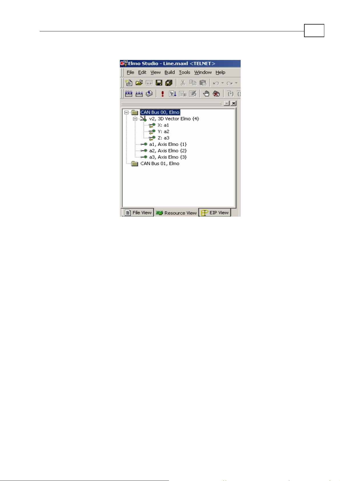
1.3.3.2 Examples of three-dimensional spline interpolatio n

For 3D vector motion, there must be a defined resource file with a vector built from three axes. In the Elmo Studio it can be defined as shown in the picture below.

Maestro Motion Library Tutorial

MAN-INTUG (Ver. 1.7)

7

Figure 1-2: Resources for the 3D vector

Example (Motion Mathematic Lib Samples\ Vector_3D \ Spline_3D – www.elmomc.com)

A spline curve throws a number of arbitrary points

SetAxisStartPos(a1, 0) //set coordinate x to 0

SetAxisStartPos(a2, 0) //set coordinate y to 0

SetAxisStartPos(a3, 0) //set coordinate y to 0

v2.vsp = 50000

v2.vse=0

v2.splines() // start spline sequence

v2.splinep(0, 0, 0) // add spline 3D point

v2.splinep(50000, 100000, 150000) // add spline 3D point

v2.splinep(100000, 50000, 100000) // add spline 3D point

v2.splinep(200000, 150000, 50000) //add spline 3D point

v2.splinee(0) // end spline sequence

Three-dimensional picture can be drawn in Matlab with the use of the following Matlab operators

[n, posX, velX, posY, velY, posZ, velZ, t] = textread('D:\Dir_22_01\trj_file', '%d %d %d %d %d

%d %d %d ', -1) where 'D:\Dir_22_01\trj_file – full path to the PVT table file.

Maestro Motion Library Tutorial

MAN-INTUG (Ver. 1.7)

For this operator to work properly, the first line of the PVT table containing a text header must be removed.

plot3(posX,posY,posZ)

axis square; grid on

8

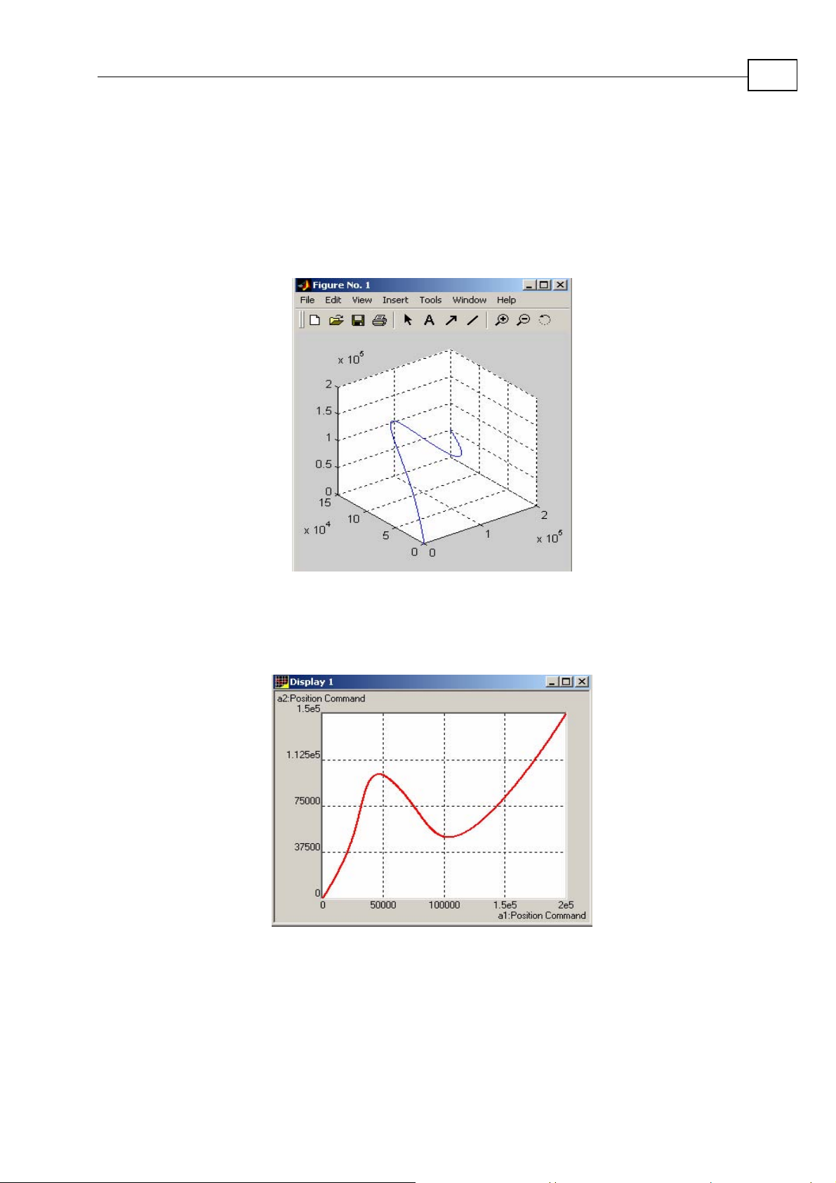
Figure 1-3: Three-dimensional picture corresponding to the calculated

PVT table (drawn in Matlab)

Results of the recording

Figure 1-4: Projection on the XY plane

Maestro Motion Library Tutorial

MAN-INTUG (Ver. 1.7)

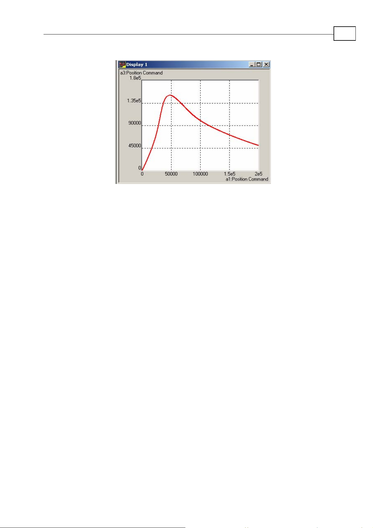
Figure 1-5: Projection on the XZ plane

9

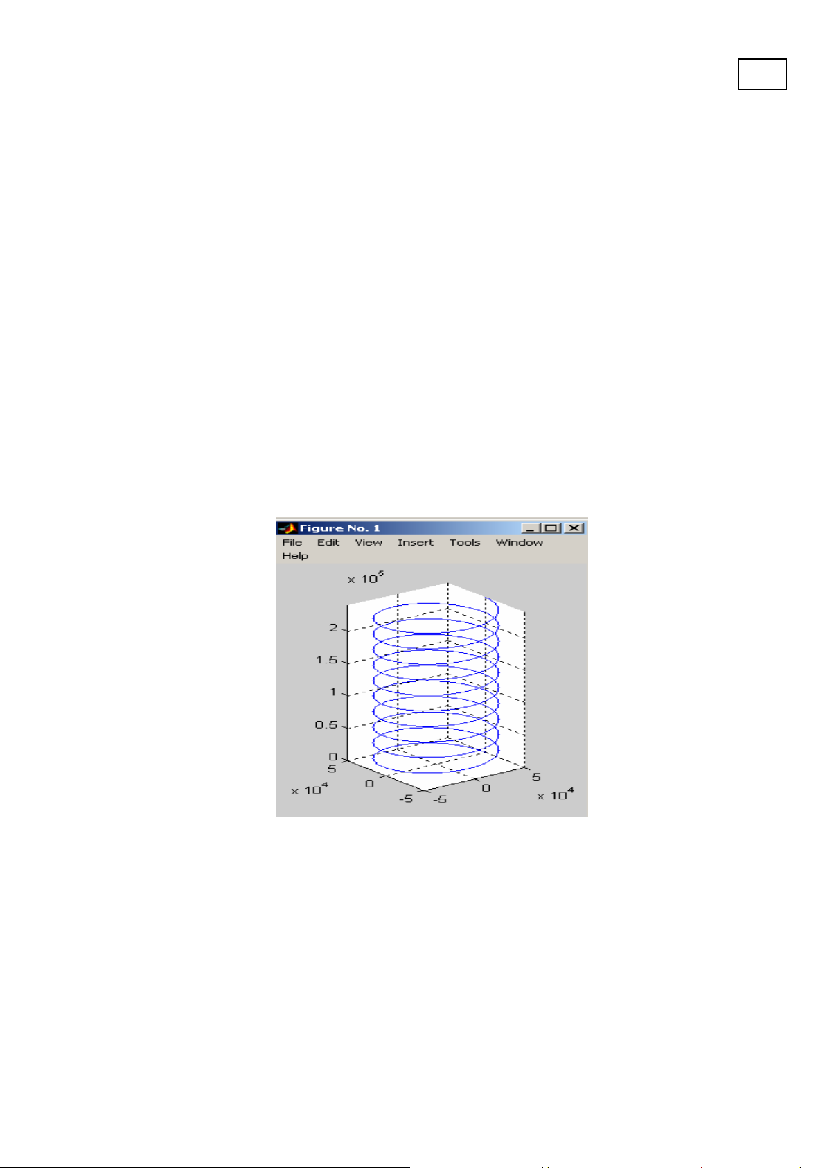
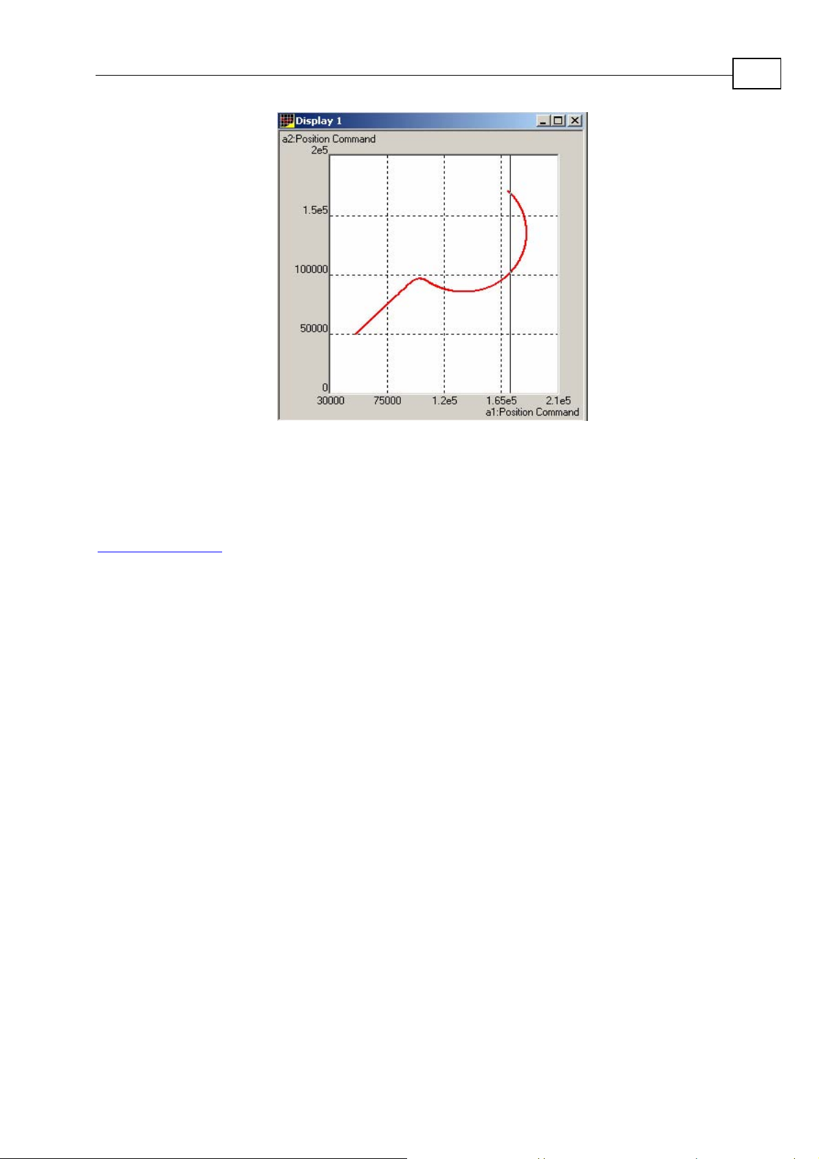
Example (Motion Mathematic Lib Samples\ Vector_3D \ Helix – www.elmomc.com)

Helix curve built with the use of the spline interpolation.

SetAxisStartPos(a1, 50000) //set coordinate x to 0

SetAxisStartPos(a2, 0) //set coordinate y to 0

SetAxisStartPos(a3, 0) //set coordinate y to 0

v2.vsp = 50000

v2.vse=0

alpha = 0 //start angle degrees

beta = 3600 // sweep angle degrees

R = 50000

H = 250000 // height

X = 50000 // start pos x

Y = 0 // start pos y

Z = 0 // start pos z

n = 120 // num points

Teta = pi*(alpha/180) //radian

dTeta = (pi*(beta/180))/n // teta increment for one step

dZ = H/n //z increment for one step

Xc = X - R*cos(Teta) // X coordinate of the helix axis

Maestro Motion Library Tutorial

MAN-INTUG (Ver. 1.7)

Yc = Y - R*sin(Teta) // X coordinate of the helix axis

v2.splines() // start spline sequence

for i=0:1:n

v2.splinep(X,Y,Z) // add spline 3D point

Teta = Teta + dTeta // calc teta for the next point

X = Xc + R*cos(Teta) // calc X coordinate for the next point

Y = Yc + R*sin(Teta) // calc Y coordinate for the next point

Z = Z + dZ // calc Z coordinate for the next point

end for

v2.splinee(0) // end spline sequence

v2.bg // begin motion

Figure 1-6: Helix three-dimensional picture for the calculated PVT table drawn in MATLAB

10

1.3.4 Polyline

To build a polyline, the Maestro user program applies the following calls to the motion library functions:

vector_name.starts(trj_name) – starts the polyline trajectory sequence with saving the PVT table built by the Motion Library in a file named trj_name. Parameter trj_name can be missed – in this case trajectory is saved in a temporary file named vector_name.trj.

vector_name.ends() - ends the polyline trajectory sequence.

Maestro Motion Library Tutorial

MAN-INTUG (Ver. 1.7)

Inside the polyline operator parenthesis vector_name.starts(trj_name) and vector_name.ends() can be added function calls – addline(), addcircle(), addsplinep() and adddwell() to define polyline segments.

For the 2D polyline vector_name.addline (int PosX, int PosY) – adds a line segment

PosX, PosY - destination position of the linear segment (counts)

vector_name.addcircle(int Radius, float StartAngle, float SweepAngle) – adds circle arc

segment

Radius - radius of the circle segment (counts)

start_angle - start angle of the circle segment (degrees)

sweep_angle - sweep angle of the circle segment (degrees)

vector_name.addsplinep(int x, int y) - adds two-dimensional spline point

11

Important note: The user should take into account that the last point of the previous segment or the first point of the trajectory is automatically added to the spline. The minimal number of the

addsplinep() operators that define the same spline segment inside the polyline must be great equal

2. This requirement is valid for every spline segment inside the polyline – not only for the first one.

For the 3D polyline

vector_name.addline (int PosX, int PosY, int PosZ) – adds a line segment

PosX, PosY, PosZ - destination position of the linear segment (counts).

vector_name.addsplinep(int x, int y, int z) - adds three-dimensional spline point

As in a two-dimensional case, the last point of the previous segment is automatically added to the spline segment and the number of points defining the spline segment cannot be less than 2.

For 2D and 3D polyline

vector_name.adddwell(delay_time) – adding delay (station) between two segments

delay_time - delay value in millisecond

Smooth transition from one curve to another inside polyline.

There are four modes that define transition from one shape to another that are defined by the parameter (vector property) vsc:

1. vsc = 0 - switch arc is not built

2. vsc = 1 – ML builds switch arc with switch radius minimally radius that satisfies kinematics

constraint r > (vse)

vse – parameter that defines end velocity on the segment preceding switch arc

vac – parameter that defines maximum vector acceleration

vae – parameter that defines admissible error for the vector acceleration

2

/[vac*vae] where

Maestro Motion Library Tutorial

MAN-INTUG (Ver. 1.7)

3. vsc = 2 – ML builds switch arc with the switch radius vsr

(this parameter must be set by the user).

4. vsc = 3 - ML builds a switch arc with the switch radius implicitly pre-defined via parameter

vsd (distance along the line from the intersection point). Parameter vsd must be set by the user.

For vsc = 2 and vsc = 3, the user can check if the values of the parameters vsr and vsd satisfy geometric constraints. Such a check can be done with the use of algorithms described in chapter 2 of this document.

Switch arc building is also influenced by the previous segment end velocity defined by the parameter (vector property) vse.

1.3.4.1 Examples for the two-dimensional polyline

Example (Motion Mathematic Lib Samples\ Vector_2D \ LineCircle – www.elmomc.com)

12

v1.vac = 28000000 //max vector acceleration

v1.vdc = 28000000 // max vector deceleration

v1.vum = 1 // build trajectory in max velocity mode

v1.starts() // begin polyline trajectory

v1.vsp = 50000 // max velocity for the line segment

v1.vse = 50000 // end velocity

v1.addline(100000, 100000) // request to add line shape

v1.vse = 0 // end velocity for the circle segment

v1.vsc = 2 // smooth intersection with fixed switch radius

v1.vsr = 10000 // switch radius

v1.addcircle(50000,225,180) //request to add circle arc shape

v1.ends() // ends polyline trajectory

Maestro Motion Library Tutorial

MAN-INTUG (Ver. 1.7)

13

Figure 1-7: Recording of the polyline trajectory

Any trajectory generated by the Motion Library (single shape or polyline) can be rotated relative to init point due to vector property vra – rotation angle in degrees.

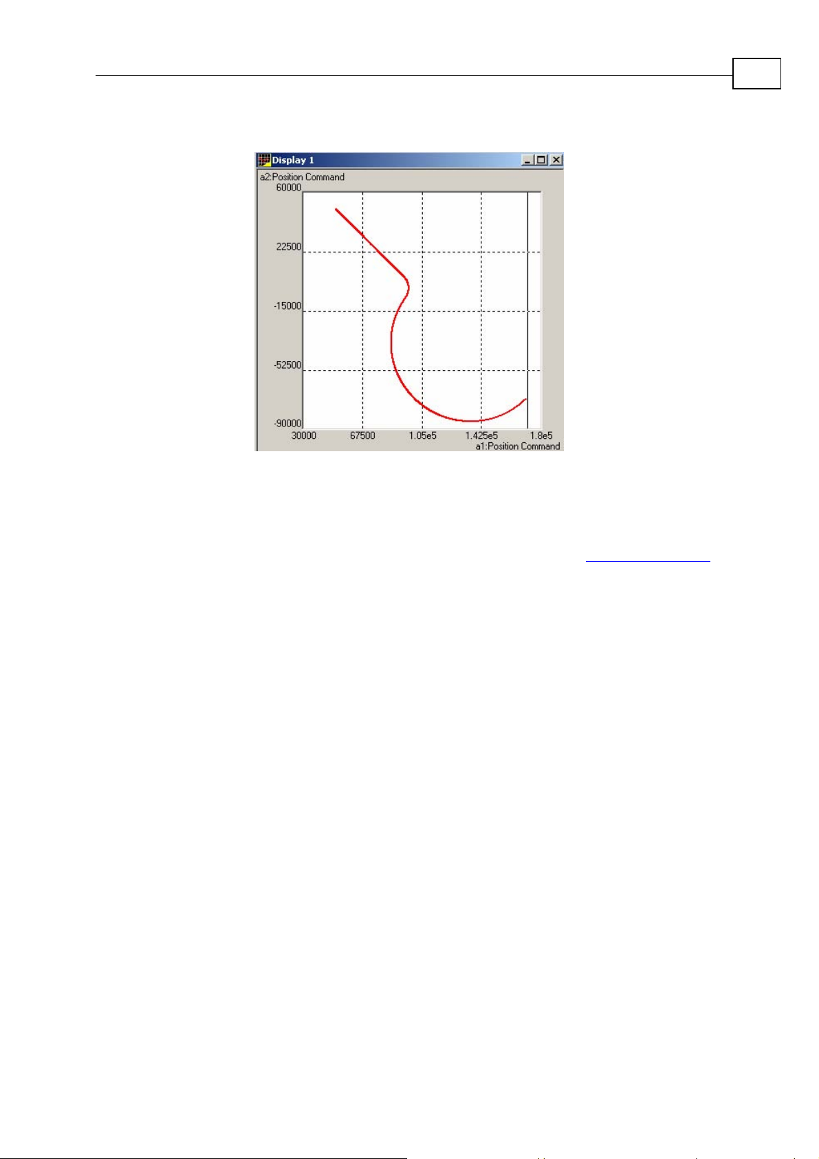
Example (Motion Mathematic Lib Samples\ Vector_2D \ LineCircleRotated –

www.elmomc.com)

// The same polyline rotated at –90 degrees relative to init point

v1.vac = 28000000 //max vector acceleration v1.vdc = 28000000 // max vector deceleration v1.vum = 1 // build trajectory in max velocity mode v1.vra = -90 // rotate spline 90 degrees relative to init point

v1.starts() // begin polyline trajectory

v1.vsc = 2 // smooth intersection with fixed switch radius

v1.vsp = 50000 // max velocity for the line segment

v1.vse = 50000 // end velocity

v1.addline(100000, 100000) // request to add line shape

v1.vsp = 50000 // maximum velocity for the circle segment

v1.vse = 0 // end velocity for the circle segment

v1.vsr = 10000 // switch radius

v1.addcircle(50000,225,180) //request to add circle arc shape

v1.ends() // end polyline trajectory

Maestro Motion Library Tutorial

MAN-INTUG (Ver. 1.7)

14

Figure 1-8: Recording of the rotated polyline

1.3.4.2 Examples for the three-dimensional polyline

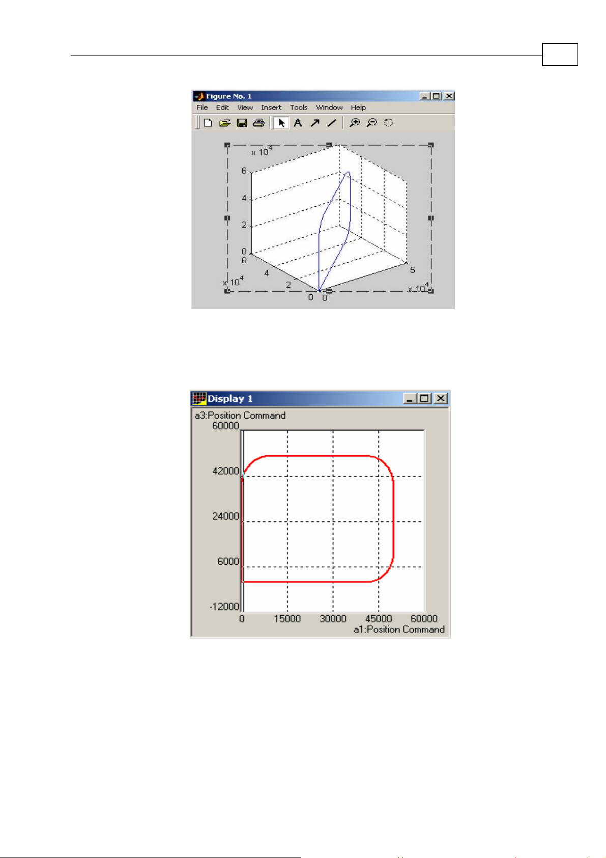
Example (Motion Mathematic Lib Samples\ Vector_3D \ Rectangle – www.elmomc.com)

Three-dimensional rectangle

SetAxisStartPos(a1, 0) //set coordinate x to 0

SetAxisStartPos(a2, 0) //set coordinate y to 0

SetAxisStartPos(a3, 0) //set coordinate y to 0

v2.vsc=2

v2.vsr=12000

v2.vsp = 70000 //max. vector velocity

v2.vse = 70000

v2.starts()

v2.addline(50000, 50000, 0) //create line from current point to coordinate

v2.addline(50000, 50000, 50000)

v2.addline(0, 0, 50000)

v2.vse = 0

v2.addline(0, 0, 0)

v2.ends()

Maestro Motion Library Tutorial

MAN-INTUG (Ver. 1.7)

Figure 1-9: Three-dimensional polygon drawn in Matlab

15

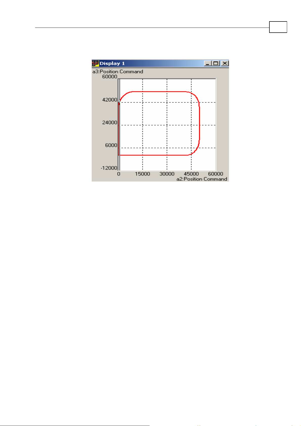
Results of the recording

Figure 1-10: Projection on the XZ plane

Maestro Motion Library Tutorial

MAN-INTUG (Ver. 1.7)

16

Figure 1-11: Projection on the YZ plane

1.4 Transition to a new trajectory with a non-zero velocity

If a transition from one trajectory to another (for instance from a line to a circle) must be executed with a velocity not equal to zero at the switch point, the Motion Library builds a switch curve to achieve smooth modification of the velocity. Such a curve is implemented as a circle arc.

As a geometrical object switch arc is completely defined by:

• radius

• coordinates of the two limit points (

where (

(

• center coordinates (X

The radius

r

X

last

first

, Y

) – last point on the first shape

last

, Y

) – first point on the second shape

first

)

o,Yo

r of the switch arc can be:

X

last

, Y

) and (X

last

first

, Y

first

)

1. Explicitly pre-defined by the user (vsc = 2, vsr defined).

In this case, it must obey the following restriction:

r ≥ (V

where

AC

) 2/AC

end

V

- end velocity at the switch point,

end

v -

v

vector acceleration.

(1-1)

Maestro Motion Library Tutorial

MAN-INTUG (Ver. 1.7)

17

In fact, the value defined as r ≥ (vse) the calculations.

Implicitly pre-defined by the user via smooth distance d along the line from the intersection

2.

point (vsc = 3, vsd defined). This mode can be implemented to the line – line, circle – line and line – circle trajectory intersections.

3. Calculated as a minimal possible for the given end velocity V

AC

Regardless of the

switch arc is considered to be uniform with the constant tangent velocity angle velocity

(vsc = 1).

v

r definition (pre-defined by the user or calculated by (1-1)) movement along the

2

/(vae*vac )

(by default vae = 0.9) must be used in

and vector acceleration

end

V = V

and constant

end

ω = V/r (1-2)

The intersection geometry imposes constraints on the switch arc radius. So the switch radius in use

r must satisfy

(V

) 2/AC

end

< r < r

v

max

(1-3)

Chapter 2 will consider all cases of the two shapes intersections and methods for the calculation of

the switch

As a base value for the switch velocity is taken the preceding segment end velocity V by the parameter vse. This value is considered as a limiting parameter that cannot be exceeded but

can be decreased. It’s also valid in case that polyline segments (preceding switch arc and the following) are executed in the fixed velocity mode (vum = 3).

In switch mode vsc = 1, the initial value of a switch velocity equal vse and can be decreased to build a switch arc trajectory equal to the integer number of PVT steps or milliseconds.

In switch mode vsc = 1, the radius of the switch arc is calculated as a minimal possible for the intersection geometry and given vector acceleration/deceleration (input parameters vac/vdc) meaning that the calculated value satisfies account the requirement to build switch arc trajectory equal to an integer number of PVT steps. The Motion Library is trying to build switch arc trajectory with velocity as close to the value given by the parameter vse for the preceding segment as possible. The switch arc (or two arcs on both ends of the segment) can take up almost all segment length that sometimes makes trajectory calculation impossible.

As an example consider the following: segment initial velocity equal

radius limit value r

max.

defined

end

(1-3). While the switch arc calculation is also taken into

Vo, end velocity V

and

e

min(V

(where ΔL – the length of the segment truncated by switch arcs, ΔT – standard PVT step). When

defining switch radius (input parameter vsr) for vsc = 2 mode or end velocity (input parameter vse) for vsc = 1 mode, the user must take into account that it can significantly influences the whole trajectory and in fact replaces the main part of a particular segment by switch arcs.

)ΔT > ΔL (1-4)

o,Ve

Maestro Motion Library Tutorial

MAN-INTUG (Ver. 1.7)

Input parameters and intersection geometry define the influence of a switch arc on a trajectory. The main cases of shapes intersection are considered below. Here as an example to consider two lines intersection. If an angle between two lines is small, even a switch arc with a small radius can significantly change initial trajectory while an arc with the same radius can be insignificant for lines

with intersection angle close to

180

o

.

In addition to geometric constraints, the Motion Library imposes limitations on the switch arc length. Each switch arc should not exceed 50% of the segment length. If there are two switch arcs adjacent to some polyline segment, then both arcs should not take more than 80% of its initial length.

18

Motion Library Tutorial Switch Radius Calculation

MAN-MLT (Ver 2.0)

Chapter 2: Switch Radius Calculation

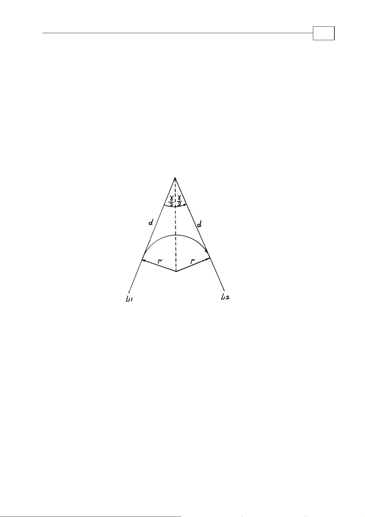
2.1 Line – line intersection

2-1

If a trajectory contains a switch from line L of the vector velocity cannot be changed at the one intersection point. To implement such a

switch, insert into a trajectory an additional element – circle arc is inserted into a trajectory (see-Figure 2-1).

The switch arc radius must satisfy (1-1).

to line L

1

with non-zero velocity, the direction

2

Figure 2-1

In the case of a line-line intersection, parameters

equation

r and d are connected by the simple

r = d*tg(γ/2) (2.1-1

where γ = π – α (α - angle between vectors L

and L2) so the pre-defined parameter

1

vsd = d must satisfy

vsd ≥ (V

If ΔL1 is the length of the line L1 and ΔL2 is the length of the line L2, then there is an evident geometric constraint for the switch radius r

r

≤ min(ΔL1, ΔL

max

(2.1-3)

In fact, due to additional limitations (50% of the segment length) used in ML, the following should be used

)2/[ACv tg(γ/2)]

end

)*tg(γ/2)

2

(2.1-2)

Motion Library Tutorial Switch Radius Calculation

MAN-MLT (Ver 2.0)

2-2

vsr ≤ min(0.5ΔL1, 0.5ΔL

(2.1-4)

)*tg(γ/2)

2

and kinematics constraint

V

end

(2.1-5)

≤ [r*vae*ACv)]

1/2

where vae – acceleration error (default value – 0.9).

So the user defined parameters must satisfy

vse ≤ [vsr*vae*vac]

(2.1-6)

vse – segment end velocity, vsr – switch radius, vac – vector acceleration.

1/2

Example 2.1a

Line 1 is defined by its init point (50000, 70000) and end point (60000,20000). .Line 2 is defined by the init point (60000,20000) and its end point (60000,70000). Switching from Line 1 to Line 2 must be executed with a minimal switch radius (vsc = 1). The cruise velocity is defined as vsp = 50000 and the end velocity vse = 50000. Vector acceleration/deceleration vac = vdc = 500000

1. The calculated minimal switch radius that satisfies kinematics constraint is

r_min = (vse)

2

/(vac*vae) = (50000)2/(500000*0.9) = 5555.6

2. The calculated distance from the intersection point that corresponds to r_min = 5555.6

ΔX

= 60000 - 50000 = 10000, dY1 = 20000 – 70000 = -50000,

1

ΔX

= 60000 – 60000 = 0, dY2= 70000 – 20000 = 50000

2

ΔL1 = [dX12 + dY12]

= [dX22 + dY22]

ΔL

2

1/2

= [(10000)2 + (-50000)2]

1/2

= [0 + (50000)2]

1/2

= 50000

= 50990

γ = π – arcos[(ΔX1ΔX2 + ΔY1ΔY2)/(ΔL1ΔL2) = = π – arcos{[(

The distance from the intersection point corresponding to the minimal switch radius

-50000)*(0) + (-50000)*(50000)]/(50990*50000)} = 0.1974

d = r_min/tg(γ/2) = 5555.6/tg(0.5*0.1974) = 56105 d > ΔL1 and d > ΔL

geometric constraints. Possible solutions: to decrease the end velocity vse or increase vector acceleration vac. Suppose that the vector acceleration is pre-defined by the mechanical parameters of the system and decrease end velocity.

which means that the minimal switch radius does not fit the

2

d

= min(ΔL1,ΔL2) = 50000

max

Motion Library Tutorial Switch Radius Calculation

MAN-MLT (Ver 2.0)

r

_max

= d

*tg(γ/2) = 50000* tg(0.5*0.1974) = 4951

max

This value is limiting and produces singular trajectory with the switch arc that replaces

L

. So we should take some value less than limiting value 4951 for instance 0.5* r_

2

max

=

0.5*4951 = 2475. Now we can recalculate maximum end velocity (vse) that satisfies this

value:

vse = [r*vac*vae]

1/2

= [2475*500000*0.9]

1/2

= 33376

(any value less equal than 33376 can be used with the switch radius r = 2475).

Example 2.1b

Line 1 is defined by init point (50000, 70000) and end point (60000,20000). Line 2 is defined by the init point (60000,20000) and its end point (60000,70000). Switch from Line 1 to Line 2 must be executed with the pre-defined switch radius (vsc = 2). We define cruise velocity vsp = 50000 and end velocity vse = 50000. Vector acceleration/deceleration vac = vdc = 500000 and switch radius vsr = 6000

2-3

1. We calculated minimal switch radius that satisfies the kinematics constraint

r_min = (vse)

2

/(vac*vae) = (50000)2/(500000*0.9) = 5555.6

Pre-defined switch radius is greater than r_min so it satisfies kinematics constraints

2. We have to check if switch radius r_switch = 6000 satisfies geometric constraints

ΔX

= 60000 - 50000 = 10000, dY1 = 20000 – 70000 = -50000,

1

ΔX

ΔL1 = [dX12 + dY12] ΔL

= 60000 – 60000 = 0, dY2= 70000 – 20000 = 50000

2

= [dX22 + dY22]

2

1/2

= [(10000)2 + (-50000)2]

1/2

= [0 + (50000)2]

1/2

= 50000

= 50990

γ = π – arccos[(ΔX1ΔX2 + ΔY1ΔY2)/(ΔL1ΔL2) =

= π – arccos{[(-50000)*(0) + (-50000)*(50000)]/(50990*50000)} = 0.1974

The distance from the intersection point that corresponds to the r_switch = 6000

d = r_switch/tg(γ/2) = 6000/tg(0.5*0.1974) = 60593

The calculated value exceeds not fit geometric constraints and must be decreased:

ΔL

1

and

ΔL

meaning that the chosen switch radius does

2

r

= min(ΔL1, ΔL

_max

)tg(γ/2) = 50000*tg(0.5*0.1974) = 4951.

2

It is possible to choose any value r_switch that satisfies r_min < r_switch and r_switch < r_max but in this case r_min > r_max. So as r_switch, use 0.9min(r_min , r_max) =

4455.9.

The chosen value exceeds

r_min so it does not fit the kinematics constraints and the end

velocity must be decreased:

Motion Library Tutorial Switch Radius Calculation

MAN-MLT (Ver 2.0)

2-4

vse = [r_switch*vac*vae]

1/2

= [4455.9*500000*0.9]

1/2

= 44778.9

Example 2.1c

(Motion Mathematic Lib Samples \Line To Line\LineLineMinRad_Ex_2c www.elmomc.com)

Line 1 is defined by its init point (300000, 900000) and end point (700000,200000). Line 2 is defined by the init point (700000,200000) and its end point (1100000,700000). Switch from Line 1 to Line 2 must be executed with the minimal switch radius (vsc = 1). We define the cruise velocity vsp = 50000 and the end velocity vse = 50000. Vector acceleration/deceleration is vac = vdc = 28000000.

1. We calculate the minimal switch radius that satisfies kinematics constraint by

r_min = (vse)

2. Geometric description of the two lines intersecting:

ΔX1 = X12 – X11 = 700000 - 300000 = 400000

ΔY

= Y12 – Y11 = 200000 – 900000 = -700000

1

2

/(vac*vae) = (50000)2/(28000000*0.9) = 99.2

ΔX

ΔY

= X22 – X21 = 1100000 – 700000 = 400000

2

= Y22 – Y21 = 700000 – 200000 = 500000

2

The length of the first line segment

ΔL1 = [ΔX

2

1

+ ΔY

2]1/2

= [4000002 + (-700000)

1

2]1/2

= 806225.8

The length of the second line segment

ΔL

= [ΔX

2

+ ΔY

An angle between two lines can be calculated as

2]1/2

= [4000002 + 5000002]

1

1/2

= 640312.4

γ = π – arccos[(ΔX1ΔX2 + ΔY1ΔY2)/(ΔL1ΔL2) = = π – arccos{[

1.193887 = 68.4

The distance from the intersection point corresponding to the minimal switch radius

400000*400000 + (-700000)( 500000)]/(806225.8*640312.4)}=

o

d = r_min/tg(γ/2) = 99.2*tg(0.5*1.193887)= 145.95

We see that d < ΔL

constraints.

and d < ΔL

1

so the calculated switch radius satisfies the geometric

1

Example 2.1d

(Motion Mathematic Lib Samples\Line To Line\LineLineFixedDist_Ex_2d – www.elmomc.com)

Motion Library Tutorial Switch Radius Calculation

MAN-MLT (Ver 2.0)

Line 1 is defined by its init point (300000, 900000) and end point (700000,200000). Line 2 is defined by the init point (700000,200000) and its end point (1100000,700000). Switch from Line 1 to Line 2 must be executed with a distance from the intersection point pre-defined by the user vsc = 3, vsd = 20000. We define cruise velocity vsp = 50000 and end velocity vse =

50000. Vector acceleration/deceleration vac = vdc = 28000000

1. We calculate the minimal switch radius that satisfies the kinematics constraint

2-5

r_min = (vse)

2

/(vac*vae) = (50000)2/(28000000*0.9) = 99.2

2. Geometric description of the two lines intersecting:

ΔX1 = X12 – X11 = 700000 - 300000 = 400000

ΔY1 = Y12 – Y11 = 200000 – 900000 = -700000

ΔX

= X22 – X21 = 1100000 – 700000 = 400000

2

ΔY2 = Y22 – Y21 = 700000 – 200000 = 500000

The length of the first line segment

ΔL1 = [ΔX

2

1

+ ΔY

2]1/2

= [4000002 + (-700000)

1

The length of the second line segment

ΔL2 = [ΔX

2

+ ΔY

Notice that d < ΔL1 and d < ΔL

2]1/2

= [4000002 + 5000002]

1

1/2

An angle between the two lines can be calculated as

γ = π – arcos[(ΔX1ΔX2 + ΔY1ΔY2)/( ΔL1ΔL2)] =

2]1/2

= 806225.8

= 640312.4

= π – arcos{[400000*400000 + (-700000)( 500000)]/(806225.8*640312.4)}=

1.193887 = 68.4

The switch radius corresponding to the given d can be calculated as

o

r=d*tg(γ/2) = 20000tg(0.5*1.193887) = 13593

1. Check the kinematics constraints. A minimal switch radius that fits kinematics

constraints can be calculated as

r

> vse*vse/(vac*vae) = 50000

min

The implicitly pre-defined switch radius is 13593 >> r

A number of similar examples with a different set of user defined and calculated parameters are considered in the Motion Mathematic Lib Samples examples TwoLinesFixDist_Fx2D_1 - TwoLinesFixDist_Fx2D_2.

2

/(28000000*0.9) = 99.2

min.

Motion Library Tutorial Switch Radius Calculation

MAN-MLT (Ver 2.0)

2.2 Circle – line intersection

Note: C – circle arc, L – line, R – circle radius, r – switch arc radius, (Xc,Yc) - circle center, (X

, Yi) – intersection point, (X

i

the line L, d – distance from point (X coordinates.

There are three possible cases that influence the calculation of parameters that define a switch arc: initial circle center and switch arc center belong to the same half-plane, initial

circle center and switch arc center belong to different half-planes (defined by the line and when the line (or continued line) moves through the center of the initial circle. For each

of these three cases, two sub cases are possible: from the point of intersection the line goes either outside or inside the circle.

Circle – line intersection geometry must satisfy some necessary conditions for the switch

arc to be built.

On the first stage of calculations we define switch arc radius. It can be predefined by the user

or calculated as

-admissible acceleration error switch arc radius can be calculated as described in 2.2.2

V2/(vae*ACv), where V – end velocity and AC

, Y

last

) – last point on the circle (X

last

, Yi) to point (X

i

first

, Y

first

), (Xo,Yo) – switch arc center

first

, Y

) – first point on

first

vector acceleration, vae

v

. If the intersection was defined by the distance d than the

L),

2-6

No matter how a switch arc radius was defined it must be coordinated with a circle and a line parameter

2.2.1 Line goes inside the circle

2.2.1.1 Switch arc center and circle center belong to two different half planes defined by the line L

The switch arc radius must obey

(vse)2/(vac*vae) < vsr < (R – h)/2 (2.2.1.1-1)

where

circle center on the line acceleration error.

This condition is necessary but not always sufficient. It’s sufficient only in the case that the

projection point

and the point of intersection of the continued perpendicular with the circle (point

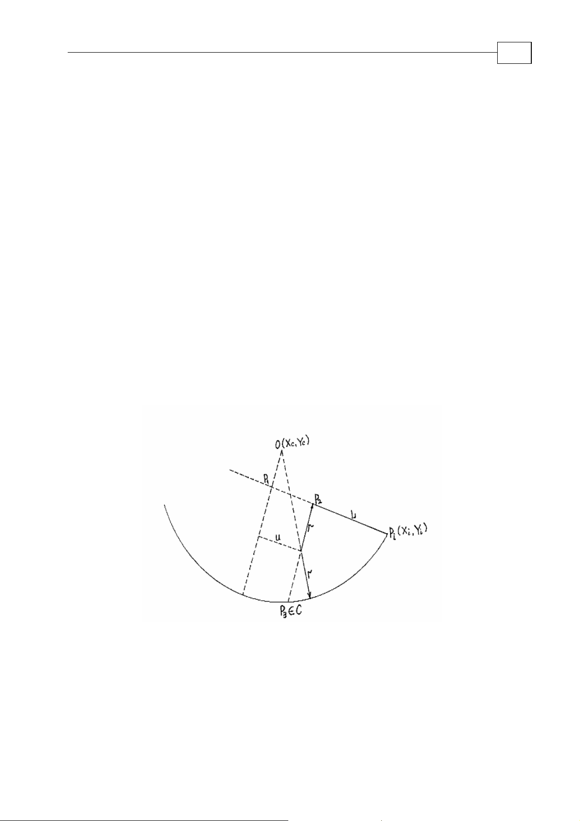
Figure 2-2) belongs to the circle arc

If one of these conditions is not fulfilled, the maximum possible switch radius r must be recalculated due to intersection geometry. Possible cases are considered below.

R - radius of the initial circle, h – the length of the perpendicular dropped from the

L, vsr - parameter that defines switch arc radius, vae – admissible

P

of the circle center on the line belongs to the line segment (P

1

∈ L)

1

P

in

2

(P2 ∈ C).

Motion Library Tutorial Switch Radius Calculation

MAN-MLT (Ver 2.0)

2-7

Figure

2-2

Example 2-2

(Motion Mathematic Lib Samples\Circle to Line\ Section 2_2_1_1\

CircleLine_Ex_2_2 – www.elmomc.com)

Circle arc is defined by its init position X angle α = 90

o

(with axis X positive direction), and sweep angle = 180o. Line end point X

from

= 0, Y

= 100000, radius R = 100000, init

from

= -140000, Yto = 100000.

Circle center coordinates

Xc = X

Yc = Y

– Rcos(απ/180) = 0 – 100000cos(π/2) = 0

from

– Rsin(απ/180) = 100000 – 100000sin(π/2) = 0

from

Circle end points X

= Xc + Rcos(α + β) = 0 + 100000cos(π/2 + π) = 0

1

Y

= Yc + Rcos(α + β) = 0 + 100000sin(π/2 + π) = -100000

1

to

Projection of the circle center on the line (Appendix )

K

= (Y2 – Y1)/(X2 – X1) = (100000+100000)/(-140000-0)=-1.4286

1

K = -1/K

Xp=(Yc – Y

= 0.7

1

+ K1*X1 - KXc)/(K1 - K) =

1

(0+100000 + 0.7*0 +1.4286*0))/(-1.4286 - 0.7) = -46979

Motion Library Tutorial Switch Radius Calculation

MAN-MLT (Ver 2.0)

Yp = Yc + K*(Xp – Xc) = 0 +0.7*(-46979 - 0) = -32885

And the perpendicular length

2-8

h = [(Xc – Xp)

2

+ (Yc - Yp)2]

1/2

= [(0 + 46979)2 + (0 + 32885)2]

1/2

= 57345

Max switch radius calculated by (2.2.1.1-1)

Rmax = (R – h)/2 = (100000 – 57345)/2 = 21328

Rmin = 100000

2

/(2800000*0.9) = 396.8

As a switch radius we can take any value Rswitch that satisfies

Rmin < Rswitch < Rmax

We take Rswitch = (Rmin + Rmax)/2 = (21328 + 396.8)/2 = 10862

In Figures 2-3 and 2-5, two possible cases are presented when the projection of the circle

center on the line

In Figure 2-3, perpendicular at the Line

P

that belongs to the circle arc P

3

maximum possible radius

L does not belong to the line segment.

L end point P

C. In Figure 2-3, observe the switch arc with the

∈

3

intersects with the circle C at point

2

r. This limit value can be calculated.

Since the coordinates of point

Figure

P1(X1,Y1) – projection of the circle center point

2-3

O(Xc,Yc) on line L and line end point P2(X2,Y2) are known, the distance is ρ(P1,P2) = u = [(X2 – X1)2 + (Y2 – Y1)2]

(2.2.1.1-2)

1/2

Motion Library Tutorial Switch Radius Calculation

MAN-MLT (Ver 2.0)

The length of the perpendicular h should also be calculated. By knowing the line equation in a form

Ax + By + C = 0 (2.2.1.1-3)

then

h can be calculated by

2-9

h = |AXc + BYc + C|/(A2 + B2)

If line

L is defined by its starting point (X1,Y1) and end point (X2,Y2), coefficients

1/2

(2.2.1.1-4)

A,B,C can be calculated by formulas in Appendix 2 or Appendix 1.

To define

r we can use an equation

(R – r)2 = (h + r)2 + u2 (2.2.1.1-5) R2 – 2Rr + r2 = h2 + 2hr + r2 + u

= (R

2

– h2 – u2)/(2R + 2h) (2.2.1.1-7)

r

max

This means that the parameter vsr that defines switch arc radius must obey the following constraints:

2

(2.2.1.1-6)

(vse)2/vac < vsr < (R2 – h2 – u2)/(2R + 2h)

(2.2.1.1-8)

The switch arc with parameter vsr calculated by (2.2.1.1-7) takes up the whole line segment. To satisfy additional requirement that switch arc cannot take more than 50% of the segment

length instead of the line end point we should use in calculations some other point

belongs to the line segment. The distance between this point and the intersection point

P2′

that

ρ

2 =

ρ(Pi,P2) must be equal k*l (where k < 0.5 , l – the length of the line). If the distance from the

intersection point Pi to P function of the used partial length k*l of the line L.

is defined as ρ(P

1

), then (2.2.1.1-7) can be presented as a

i P1

= [R

2

– h2 – (ρ(Pi P1) – k*l)2]/(2R + 2h)

r

(2.2.1.1-9)

max

Example 2-4

(Motion Mathematic Lib Samples\Circle to Line\ Section 2_2_1_1\

CircleLine_Ex_2_4 – www.elmomc.com)

Circle arc (Figure 2-4) is defined by its init position X init angle α = –90 point X

50000) so the line L is parallel to the axis X. From Figure 2-4, h = 50000, u = 25000. The switch radius is calculated by (2.2.1.1-7).

= 25000, Yto = 50000. Circle end point [Xc + Rcos(-30), Yc + Rsin(-30)] = (86603,

to

r = 0.5*(1000002 – 500002 – 25000

o

(with axis X positive direction), and sweep angle = +60o. Line end

2

)/(100000 + 50000) = 22917

from

= 0, Y

= 0, radius R = 100000,

from

Motion Library Tutorial Switch Radius Calculation

MAN-MLT (Ver 2.0)

2-10

Figure

2-4

In our calculations was not taken in account additional requirement that the switch arc should not take more than 50% of the segment length. So the calculated switch arc with the radius 22917 takes the whole line segment.

If in the calculations, some point on the line is used, for example (65000, 50000), instead of the line end point, then u = 65000 and the result is:

r = 0.5*(1000002 – 500002 – 65000

Perpendicular to the Line L end point P

In Figure 2-5, there is an intersecting geometric figure showing that a perpendicular line at

Line L end point P

is a switch arc with a maximum possible radius

By knowing the coordinates of a circle center O(X

it is possible to find an intersection point P

the length of the line segment

does not intersect the circle arc C. The switch arc drawn in Figure 2-5

2

P3P6: ρ1 = ρ(P3, P6).

2

)/(100000 + 50000) = 10917

does not intersect the circle arc C

2

r.

) and a circle init point P6(X6,Y6)

c,,Yc

of two lines: (X

3

) – (X6,Y6) and L and

c,Yc

Drop a perpendicular from point P

= ρ(P6, P4). To define r, use a proportion

ρ

2

r/ρ

= (ρ1 – r)/ρ1

2

(2.2.1.1-9)

and finally

on the line L and by (2.2.1.1-4) define its length

6

Motion Library Tutorial Switch Radius Calculation

MAN-MLT (Ver 2.0)

2-11

r = ρ

As in the previous case, the user defined parameter vsr must obey

(vse)2/vac < vsr < ρ

/(ρ1 + ρ2) (2.2.1.1-10)

1ρ2

/(ρ1 + ρ2) (2.2.1.1-11)

1ρ2

Figure

2-5

Example 2-6

(Motion Mathematic Lib Samples\Circle to Line\ Section 2_2_1_1\

CircleLine_Ex_2_6 – www.elmomc.com)

The circle arc in Figure 2-6 is defined by the radius R = 100000, init angle α = -90 sweep angle β = 30

Line L end point: X The circle arc end point P

= R*sin(-π/3) = -86602.54;

Y

5

o

and the init position X

= -40000, Yto = 0;

to

coordinates can be calculated as X5 = R*cos(π/3) = 50000,

5

from

= 0, Y

= -100000.

from

Line L is defined by two points P1(-40000, 0) and P2[Rcos(-60), Rsin(-60)] = P

(50000, -86602.54). Its standard equation is Ax + By + C = 0,

2

where A = – (Y

– Y1) = -(0 + 86602.54) = –86602.54, B = X2 – X1 = -40000 – 50000

2

= -90000, C = X1(Y2 – Y1) – Y1(X2 – X1) = 50000(0 + 86602) + 86602.54(-40000 -

50000) =–3464101600.0 where (X1, Y1) and (X2,Y2) – line end points. Calculate ρ2 by (3.1.1-4) as

ρ

|(-86602.54)0 + (-90000)(-100000) - 3464101600.0|/[(-86602.54)2 +(-90000)2 ]

2 =

= 44322.6596

o

,

1/2

To define ρ

take into account that line (O, P6) in Figure 2-6 coincides with the axis

1,

Y so coordinates of its intersection point with the line L are (0, -C/B).

Motion Library Tutorial Switch Radius Calculation

MAN-MLT (Ver 2.0)

ρ

= 100000 - |C/B| = 100000 - |(-3464101600.0)/(-90000)| = 61509.98222

1

2-12

r = ρ

/(ρ1 + ρ

1ρ2

) = 61509.98*44322.66/(61509.98 + 44322.66)= 25760.351

2

meaning that the switch radius in use must be less than this limiting value.

Figure 2-6

Values calculated by (2.2.1.1-7) and (2.2.1.1-10) are not recommended but limiting values. The switch radius in use must be less those values.

Such limiting values produce irregular cases of intersection. If we use (2.2.1.1-7) switch arc replaces line L and if we use (2.2.1.1-9) switch arc replaces initial arc C.

2.2.1.2Switch arc center and a circle center belong to the same half plane.

In this case (Figure 2-7), the switch radius must satisfy the following condition:

r ≤ (R + h)/2 (2.2.1.2-1)

Motion Library Tutorial Switch Radius Calculation

∈

MAN-MLT (Ver 2.0)

2-13

Figure

This condition is not always sufficient. Adequacy depends on arc and line lengths. If the

circle’s center projection on the line intersection point of the continued perpendicular with the circle arc belonging to the

circle segment

If projection of the circle init point

8), use the following proportion

P

C then (2.2.1.2-1) is sufficient.

∈

2

L belongs to the line segment (P

P1 belongs to the line segment - P

2-7

L) and an

1

∈

5

L (Figure 2-

h/r = ρ(P3, Oc)/[ρ(P1, P3) – r] = ρ1/(ρ2 – r) (2.2.1.2-2)

where P3 is the point of intersection of the line (P

the circle

perpendicular dropped from the circle center (2.2.1.2-4) or another method.

From (2.2.1.2-2) the results are

hρ2 – hr = rρ

P1 and a circle center are known, P3 can be determined. The length h of the

Oc on the line L can be also found by

1 =>

r = hρ2/(ρ1 + h) (2.2.1.2-3)

) with the line L. As init point of

1,Oc

Motion Library Tutorial Switch Radius Calculation

MAN-MLT (Ver 2.0)

2-14

Figure

2-8

Example 2-9

(Motion Mathematic Lib Samples\Circle to Line\ Section 2_2_1_2\

CircleLine_Ex_2_9 – www.elmomc.com)

The circle arc (Figure 2-9) is defined by its radius R = 100000, init angle α = 0o and sweep

angle

β = -45

In this case ρ

Circle center coordinates

o

, init point P1(100000, 0). Line target position (-40000, 0).

= 40000

1

ρ

= 140000 - line (P

,

2

) coincide with axis X.

1,P3

Xc = 100000 - Rcos(0) = 0, Yc = 0 - Rsin(0) 0.

Line init point coordinates X1 = 0 + 100000cos(0 - 45) = 70711, Y1 = 0 + 100000sin(0-

45) = -70711

To calculate the length of perpendicular h dropped from the circle center (Xc,Yc) on the line, use formulas (a1.6), (a1.4) and (a1.7) from Appendix 1.

k = (Y2-Y1)/(X2-X1)=(0+70711)/(-40000-70711)= -0.6387, q = -1/k = 1.5657

Xpr = (y - Y1 + k*X1 - q*x)/(k - q) = -11589.6, Ypr = y + q*(Xpr - x) = - 18145.7

h= [(-11589.6 - 0)

2

+ (- 18145.7 - )2]

1/2

= 21531

r = hρ2/(ρ1 + h) = (21531*140000)/( 40000 + 21531) = 48989

Motion Library Tutorial Switch Radius Calculation

MAN-MLT (Ver 2.0)

2-15

Figure

Projection of the circle arc init point

If a projection of the circle arc init point P

segment

L (Figure 2-10), calculate the maximum switch radius r using equation

2

ρ

(Oc,P5) + (r – h)2 = (R – r)2 (2.2.1.2-4)

or

)2 + (r – h)2 = (R – r)2 (2.2.1.2-5)

(ρ

1

(ρ

)2 + r2 – 2rh + h2 = R2 – 2Rr + r

1

P1 on the line L does not belong to the line segment L.

on the line L does not belong to the line

1

2

2-9

(2.2.1.2-6)

R2 – (ρ1)2 – h2 = 2Rr – 2rh (2.2.1.2-7)

The results for

= [R

2

– (ρ1)2 – h2]/(2R – 2h) (2.2.1.2-8)

r

To define

distance from

r

ρ(Oc,P5), drop a perpendicular from the circle center Oc on the line L. The

the projection point P

to the line end point P3 is equal to ρ(O

4

c,P5

).

As well as in case when the circle and switch arc centers belong to different half planes values calculated by (2.2.1.2-3) and (2.2.1.2-8) are not recommended but limiting ones. Switch radius in use must be less those values.

Motion Library Tutorial Switch Radius Calculation

MAN-MLT (Ver 2.0)

2-16

Figure

2-10

Example 2-11

(Motion Mathematic Lib Samples\Circle to Line\ Section 2_2_1_2\

CircleLine_Ex_2_11 – www.elmomc.com)

Circle arc (Figure 2-11) is defined by its init position (X = 0, Y = 60000), radius R = 60000, init angle α = 0o, and a sweep angle β = -135

o

. Line target position 25000, -42426.

Circle center coordinates (Xc, Yc) = (0 – Rcos90, 60000 – Rsin90) = (0,0). Circle end point coordinates (Xc + Rcos(-45

line L is parallel to the axis X meaning that =25000 and

r can be calculated by

o

), Yc + Rsin(-45o) = (42426, - 42426). Notice that

h = |0 - 42426| = 42426, ρ =|25000 - 0|

(3.1.2-8): r = (60000*60000 – 25000*25000 – 42426*42426)/(2*60000 – 2*42426) = 33430

Figure

2-11

Motion Library Tutorial Switch Radius Calculation

∈

MAN-MLT (Ver 2.0)

2.2.1.3 Line intersects the center of the circle

Consider the last case of the circle – line intersection: the line goes inside the circle through the center of the circle (Figure 2-12-2-15). The following cases are possible:

2-17

a) The length of the line

orthogonal to the line intersects the circle arc: evident geometric constraint on the switch arc radius is

ΔL is greater than the circle radius R and the circle diameter

P

C

(Figure 2-12). In this case an

1

r ≤ R/2 (2.2.1.3-1)

b) The length of the line

line end point intersects the circle arc:

geometric limit for the switch radius

ΔL is less than the circle radius R and a perpendicular at the

Figure

2-12

P

C

(Figure 2-13). To define the

1

r, use the following equation:

(R – r)2 = (R – ΔL)2 + r2

(2.2.1.3-2)

or

– 2Rr = – 2RΔL + ΔL

that leads to

r = (2RΔL – ΔL2)/2R = ΔL – ΔL2/(2R) (2.2.1.3-3)

2

Motion Library Tutorial Switch Radius Calculation

MAN-MLT (Ver 2.0)

2-18

Figure

2-13

Example 2-14

(Motion Mathematic Lib Samples\Circle to Line\ Section 2_2_1_3\

CircleLine_Ex_2_14 – www.elmomc.com)

The circle C1 (Figure 2-14) is defined by its init point (80000,0), radius R = 80000, init

α = 0 and a sweep angle β = -135. Line target position (-28284, -28284). The length

angle of the line segment

ΔL = 28284*2

1/2

= 40000.

The circle C1 is defined by the init point (80000,0), radius R = 80000, init angle α = 0

and a sweep angle β = 135.

Circle target position: Xend = 80000*cos(135) = - 56569, Yend = 80000*sin(-135) = -56569.

The length of the line segment

ΔL = [(-56569 + 28284)2 * 2]

Calculate the upper limit of the switch radius by (3.1.3-3): r = (2RΔL – ΔL

1/2

= 40000.

2

)/(2R) =

(2*80000*40000- 400002)/(160000) =30000

Figure 2-14

Motion Library Tutorial Switch Radius Calculation

MAN-MLT (Ver 2.0)

2-19

c) The circle arc sweeps an angle less than 90

circle init point

P

on the line L intersects line segment at point P

1

15). A projection of the circle init point

o

and a perpendicular dropped from the

P1(X1,Y1)

and the length of the segment defined by the line init point

P

: ρ

= ρ(P3,P2) can be determined. Now calculate the maximum switch radius

2

1

with the use of the following equation:

(R – r)2 = (R – ρ1)2 + r

2

(2.2.1.3-4)

that leads to

–2Rr = – 2Rρ1 + (ρ1)

2

and finally

r = [2Rρ1 – (ρ1)2]/(2R)

(2.2.1.3-5)

∈ C

2

on the line L – point P

P

and projection point

3

(Figure 2-

1

2(X2,Y2

)

Figure 2-15

Example 2-16

(

Motion Mathematic Lib Samples\Circle to Line\ Section 2_2_1_3\

CircleLine_Ex_2_16 – www.elmomc.com)

The circle (Figure 2-16 ) is defined by its init point P

α = -90

Circle end point P

o

and sweep angle β =-45o. Coordinates of the line end point (150000,150000).

(line init point) coordinates are calculated as X3 = 80000*cos(pi + pi/4) = -

3

56569 and

Y

= 80000*sin(pi + pi/4) = -56569

3

Drop a perpendicular from the circle init point P projection point P

use formulas from the Appendix 1.

2 ,

k = dY/dX = (150000 + 56569)/ (150000 + 56569) = 1, q = –1/k = –1.

(0, -80000), radius R = 80000, init angle

1

on the line L2. To define coordinates of the

1

Motion Library Tutorial Switch Radius Calculation

MAN-MLT (Ver 2.0)

By (a1.6) we have

2-20

Xp = (Yo – Y1 + kX

40000

Yo + q(X – X

Yp =

Distance

For the maximum switch radius we get from (3.1.3-5)

ρ1 = ρ(P3,P2) = [(–40000 + 56569)

– qXo)/(k – q) = (–80000 + 56569 – 56569 - 0)/(1+1) = –

1

) = -80000 – (–40000 - 0) = –40000.

o

2

+ (–40000 + 56569)2]

r = [2Rρ1 – (ρ1)2]/(2R) = [2*80000*23432 - 23432

1/2

= 23432

2

]/160000 = 20000

Figure

2-16

2.2.2 Switch arc radius calculation by the distance from the intersection point

If svc = 3 mode (vsd = d is given) is considered and it is important to know the switch arc radius r to check if end velocity and vector acceleration satisfy (1-1). If d – distance from the point (X function of parameters d and R (we have to know r to check condition 1-1).

Consider three possible cases of a circle and switch arc positions relative to the line.

) to the point (X

i,Yi

first,Yfirst

) is given, then it can be useful to re-calculate r as a

2.2.2.1 Initial circle center and switch arc center belong to the same half-plane

2.2.2.1.1 Line continues outside the circle (Figure 2-17)

As in case of the switch arc center coordinates calculation we drop a perpendicular from the

circle center

perpendicular

(Xc,Yc) on the line and get a projection point (Xp,Yp). The length of the

ρ

can be defined as

1

ρ1 = [(Xp – Xc)2 + (Yp – Yc)2]

Define point

(X1,Y1) so that

1/2

(2.2.2.1.1-1)

Motion Library Tutorial Switch Radius Calculation

MAN-MLT (Ver 2.0)

ρ[(Xp,Yp),(X1,Y1)] = r

(2.2.2.1.1-2)

The following is known:

ρ

= ρ[(Xp,Yp),(Xf, Yf)] = ρ[(Xp,Yp),(Xi, Yi)] + d

3

(2.2.2.1.1-3)

where (Xi, Yi) – circle-line intersection point .

2-21

ρ[(X1,Y1),(Xo, Yo)] = ρ[(Xp,Yp),(Xf, Yf)] = ρ

As

(R + r)

2

– (ρ3)

2

= (ρ1 – r)2

then use an equation to define r

3

(2.2.2.1.1-4)

(2.2.2.1.1-4) for r there is

From

r = [(ρ3)2 + (ρ1)2 – R2]/(2R + 2ρ1)

(2.2.2.1.1-5)

2.2.2.1.2 Line continues inside the circle (Figure 2-18)

The following is known:

ρ

= ρ[(Xp,Yp),(Xi,Yi)] – d

3

(2.2.2.1.2-1)

Figure

2-17

Motion Library Tutorial Switch Radius Calculation

MAN-MLT (Ver 2.0)

2-22

Figure

so an equation can be written

2-18

(R – r)2 – (ρ1 – r)2 = (ρ3)2 (2.2.2.1.2-2)

that produces for

r = [R

2

– (ρ3)2 – (ρ1)2]/(2R – 2ρ1) (2.2.2.1.2-3)

r

2.2.2.2 Initial circle center and switch arc center belong to two half planes defined by the line L.

2.2.2.2.1 Line continues outside the circle (Figure 2-19)

In this case

ρ

= ρ[(Xp,Yp),(Xi,Yi)] + d

3

(2.2.2.2.1-1)

Equation for r

2

(ρ

+ r)2 = (R + r)2 – (ρ3)

1

(2.2.2.2.1-2)

From (2.2.2.2.1-2) we have

r = [(ρ1)

2

+ (ρ3)

2

– R2]/(2R – 2ρ1) (2.2.2.2.1-3)

2.2.2.2.2 Line continues inside the circle (Figure 2-20)

ρ3 = ρ[(Xp,Yp),(Xi,Yi)] – d (2.2.2.2.2-1)

Equation for r

(R – r)2 – (ρ3)2 = (ρ1 + r)2 (2.2.2.2.2-2)

Motion Library Tutorial Switch Radius Calculation

MAN-MLT (Ver 2.0)

that produces

r = [R2 – (ρ1)2 – (ρ3)2]/(2R + 2ρ1) (2.2.2.2.2-3)

2-23

Figure

2-19

Figure

2-20

Figure 2-21

Motion Library Tutorial Switch Radius Calculation

MAN-MLT (Ver 2.0)

2-24

2.2.2.3 Circle center (Xc,Yc) Є L1 (line L1 intersects the center of the circle)

2.2.2.3.1 Line goes outside of the circle (Figure 2.11).

An equation for r

(R + r)2 = (R + d)2 + r2 (2.2.2.3.1-1) r = (2Rd + d2)/(2R) (2.2.2.3.1-2)

2.2.2.3.2 Line goes inside the circle (Figure 2.12)

(R – r)2 = (R – d)2 + r2 (2.2.2.3.2-1)

r = (2Rd – d2)/(2R) (2.2.2.3.2-2)

Figure

2-22

2.2.3 Line goes outside the circle

If the line goes outside of the circle, the switch arc radius is limited by the length of the line segment and the length of the circle arc segment. The connection between the switch arc

radius and distance

line

L was considered in section 3.2. The maximum switch radius for the given line

segment

ΔL can be calculated by formulas (2.2.2.1.1-5) or (2.2.2.2.1-3) from 2.2.2.1.1 where

d between intersection point and a last point of the switch arc on the

d = ΔL.

When considering the limitations imposed by the length of the circle arc (defined by the sweep angle and a circle radius), three cases are possible:

Motion Library Tutorial Switch Radius Calculation

MAN-MLT (Ver 2.0)

1. Circle init radius intersects with the line L continued in its positive direction

(Figure 2-23);

2-25

2. Line

3. Line

L is parallel to the init radius (Figure 2-25);

L continued in the reverse direction intersects init radius (Figure 2-26) (by

the init radius there a line segment that connects the circle arc center with the circle arc init point).

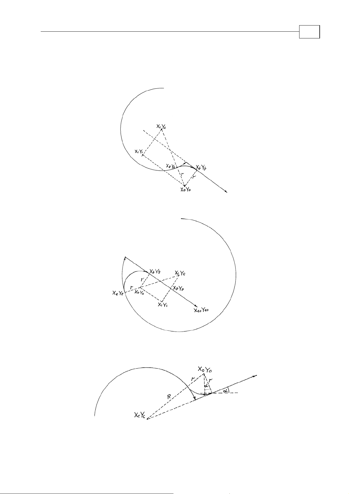
2.2.3.1 Line L and init radius continued in their positive

intersecting directions

The init circle radius continuing in its positive direction intersects with the line L continued

in its positive direction (Figure 2-23). It takes place if the circle arc init angle with the axis

positive direction

circle arc sweep angle

α is less than the line L angle with the axis X positive direction φ and the

β < 0 (β < 0, α < φ) or in case: β > 0, α > φ.

X

Figure

Drop a perpendicular from the circle center

calculated by (2.2.1.1-4). Now calculate the angle

arc radius. The circle arc sweep angle

Now calculate the distance

d = ρ(Oc, P

To define the switch radius r, use a proportion

) = h/cos(λ) (2.2.3.1-1)

2

θ so λ = θ + γ = θ + arccos(h/R).

2-23

O

on the line L. Its length h can be

c

γ = arccos(h/R), where R – circle

r/h = (d – R – r)/d (2.2.3.1-2)

Motion Library Tutorial Switch Radius Calculation

MAN-MLT (Ver 2.0)

or

rd = hd – hR – hr (2. 2.3 .1 -3 )

2-26

and for

r the result is

r = h(d – R)/(d + h ) (2.2.3.1-4)

Example 2-24

(Motion Mathematic Lib Samples\Circle to Line\ Section 2_2_3_1\

CircleLine_Ex_2_24 – www.elmomc.com)

The circle is defined by its radius R = 50000, init angle α = 45o and sweep angle β= -45

and the init point (35355, 35355). The line L end point is (80000, 80000). The circle end

angle = standard equation Ax + By + C = 0,

o

0

, so the line init point coordinates (50000, 0). For the coefficients A, B, C in the line

A = -(Y2 - Y1) = -0 + 80000 = 80000 , B = X2 - X1 = 80000 – 50000 = 30000,

C = X1(Y2 - Y1) - Y1(X2 - X1) = 50000(80000 – 0) – 0 = 4000000000. The length of h

can be calculated as:

h = |C|/(A

The length h of the perpendicular can be also calculated by formulas (a.16),(a1.4) and (a.17) from Appendix1 (this approach is used in the sample program CircLine_ex_3_13a).

2

+ B2)

1/2

= 4000000000/(80000*80000 + 30000*30000)

1/2

= 46816.5

o

β = 45

o

= π/4 = 0.785398, γ = arccos(h/R) = arccos(46816.5/50000) =

0.358768.

λ = β + γ = 0.785398 + 0.358768 = 1.144166.

d = h/cos(λ) = 46816.5/cos(1.144166) = 113136 and the for the switch radius:

r

= h(d – R)/(d + h) = 46816.5(113136-50000)/(113136 + 46816.5) = 18479

max

Motion Library Tutorial Switch Radius Calculation

MAN-MLT (Ver 2.0)

Figure 2-24

2-27

2.2.3.2 Line parallel to the circle arc init radius

a) Line direction coincides with the direction of the init radius

In this simple case (Figure 2-25) maximum switch radius is equal to the distance between

line L and circle arc init radius. This distance is equal to length of perpendicular

from the circle arc center

O

on the line L. To define it we can use the same formula

c

(2.2.1.1-4).

h dropped

Figure 2-2-25a

b) Line direction is opposite to the direction of the init radius

Motion Library Tutorial Switch Radius Calculation

MAN-MLT (Ver 2.0)

2-28

Figure 2-25b

Maximum switch radius is perpendicular to the line L at the line end point. h – the length of

the perpendicular dropped from the circle center on the line. We can calculate an angle between the perpendicular at the line end point and the line that connect the centers of the init circle and a switch arc

γ

γ = 180 – 90 – (180 – θ) = θ – 90 (2.2.3.2-1)

To define max switch radius we can use an equation

(R + r)cosγ = r + h (2.2.3.2-1)

that produces

r = (Rcosγ – h)/(1 – cosγ) (2.2.3.2-1)

2.2.3.3 Line L and init radius continued in their reverse

directions intersect

This case is shown in Figure 2-26.

1. Find the coordinates

P1(X1,Y1) – intersection point of two lines init circle radius

(Oc,P2) and a line L.

2. Knowing the coordinates of circle arc center

Oc(Xc,Yc) and intersection point

P1(X1,Y1) makes ρ1 = ρ(P1,Oc) = [(X1 - Xc)2 + (Y1 - Yc)2]

1/2

known.

Motion Library Tutorial Switch Radius Calculation

MAN-MLT (Ver 2.0)

2-29

3. Know trajectory init point P

[(X2 – X1)2 + (Y2 – Y1)2]

4. Drop a perpendicular from the circle center O

length

5. To get switch arc radius, use a proportion

ρ

1/(ρ2

(2.2.3.3-1)

h by (2.2.1.1-4)

+ r) = h/r or

2(X2,Y2

1/2

), calculate ρ2 = ρ(p2, p1) =

on the line L and calculate its

c

ρ1r = hρ2 + hr

(2.2.3.3-2)

and finally the value for r is:

r = hρ2/(ρ1 - h) (2.2.3.3-3)

Figure 2-25

Example 2-27

(Motion Mathematic Lib Samples\Circle to Line\ Section 2_2_3_3\

CircleLine_Ex_2_27 – www.elmomc.com)

The circle arc is defined by its radius R = 40000, init angle α = 30o and sweep angle β = -30o, init point (34641, 20000) – Figure 2-27.

Line L target point (130000, 25000).

Coordinates of the circle center O 40000sin(π/6) = 0;

Define the coordinates of the intersection point P

: Xc = 34641 – 40000cos(π/6) = 0, Yc = 20000 –

c

, Y1). For X1 and Y1, use expressions

1(X1

Motion Library Tutorial Switch Radius Calculation

MAN-MLT (Ver 2.0)

By (a3.6)-(a3.7) from Appendix 3.

= ΔX1/ΔY1= (34641-0)/(20000-0) = 1.73205

q

1

= ((q1*Y1 + X21 – X11)*ΔY2 –Y21ΔX2)/(q1*ΔY2 – ΔX2) =

Y

1

((1.73205*0 + 40000 –0)*(25000-0) - 0)/( 1.73205*(25000-0) - (130000-40000)) =

-21414X1 = X11 + q1 (Y1– Y11) = X1 = 0 + 1.73205(-21414- 0) = -37090

To get the length of the perpendicular h from the circle center on the line L, line L is needed.

2-30

Figure 2-26

standard equation in a form Ax + By + C = 0. For A,B,C we have

A = -(Y

C = X

h = (0*25000 + 0*90000 + 109)/( 250002 + 900002)

21414)

ρ

= [(-37090 – 34641)2 + -21414– 20000)2]

2

– Y21) = 25000, B = 130000 – 40000 = 90000, C =

22

– Y21) - Y1(X22 – X21) = 40000(25000-0) = 109.

21(Y2

2]1/2

= 42828

1/2

=82828

1/2

= 10706ρ1 = [(-37090)2 + (-

and for maximum switch radius we get

r = hρ2/(ρ

– h) = 10706*82828/(42828– 10706) = 27605

1

2.3 Circle – circle intersection

Note: C1 – first circle arc, C2 – second circle arc, Pi – point of two circle arcs intersection,

Co1 – first circle center point, C

– second circle center point.

o2

Motion Library Tutorial Switch Radius Calculation

MAN-MLT (Ver 2.0)

2.3.1 One of two circle arcs intersects the internal area of the second

2-31

If the circle arc C1 comes from inside of the circle C

C

inside the circle

r ≤ (R

(2.3.1-1)

where h = ρ(O

+ h)/2

2

P1(X1,Y1) of the line O1O

(Figure 2-28). Condition (2.3.1-1) is not always sufficient– only in cases that the points of

intersection

P2(X2.Y2)

O1O

∈

), then the switch arc radius must satisfy the necessary condition

1

) – distance from the circle C2 center O

2,P1

connecting the centers of two circles with the circle arc C

2

with C

2

C

(Figure 2-28).

2

and C

1

belong to C

2

– Figure 2-28 (or circle C

2

to the intersection point

2

and C

1

: P1(X1,Y1) ∈ C

2

continues

2

and

1

Figure 2-28

In Figure 2-29 the case when a point of intersection of the line O

the circle arc

init point arc C2 (calculation of the circle – line intersection point coordinates can be found in

Appendix 4). distance

C

is presented. Line O

1

goes through the circle C1 center O1 and its

1P1

P1(X1,Y1). P2(X2,Y2) – intersection point of the line O1P

By knowing the coordinates of two points P1 and P2, calculate the

does not belong to

1O2

with the circle

1

d = ρ(P1,P2).

To define the maximum switch arc radius

(X

– X1)/(X2 – X1) = r/d (2.3.1-2)

o

r, use the following system of equations:

(Yo – Y1)/(Y2 – Y1) = r/d (2.3.1-3)

Motion Library Tutorial Switch Radius Calculation

MAN-MLT (Ver 2.0)

(Xo – Xc2)2 + (Yo – Yc2)2 = (R2 – r)2 (2.3.1-4)

From (4.1-2)

Xod – X1d = r(X2 – X1)

2-32

and for X

X

= r[(X2 – X1)/d] + X1 = rC1 + X1 (2.3.1-5)

o

From (4.1-3)

d – Y1d = r(Y2 – Y1)

Y

o

and for Y

= r[(Y2 – Y1)/d] + Y1 = rC2 + Y1 (2.3.1-6)

Y

o

Substituting (4.5) and (4.6) into (4.4)

[rC1 + X1 – Xc2]2 + [rC2 + Y1 – Yc2]2 = (R2 – r)

or

[rC1 + C3]2 + [rC2 + C4]2 = (R2 – r)

o

2

(2.3.1-7)

2

(2.3.1-8)

(C1)2r2 + (2C1C3)r + (C3)2 + (C2)2r2 + (2C2C4)r + (C4)2 =

(R

)2– 2R2r + r

2

(2.3.1-9)

Figure 2-29

2

[(C1)2 +(C2)2 – 1] + r[2C1C3+2C2C4 + 2R2] + (C3)2 +(C4)2–(R2)2 = 0

r

(2.3.1-10)

But when considering

Motion Library Tutorial Switch Radius Calculation

MAN-MLT (Ver 2.0)

(C1)2 + (C2)2 – 1 = [(X2 – X1)/d]2 + [(Y2 – Y1)/d]2 – 1 = d2/d2 – 1 = 0

(2.3.1-11)

2

as d

= ρ2(P1,P2) = (X2 – X1)2 + (Y2 – Y1)2.

and if noting

2-33

C6 = 2(C1C

The results for r are as follows:

+ C2C

3

+ R2), C7 = (C3)2 + (C4)2 – (R2)

4

2

r = –C7/C6 (2.3.1-12)

where

C1 = (X2 – X1)/d

= (Y2 – Y1)/d

C

2

C

= X1 – X

3

= Y1 – Y

C4

C6 = 2(C1C

C

= (C3)2 + (C4)2 – (R2)

7

The maximum switch radius can be also estimated as a solution of the alternate system

c2

+ C2C

3

+ R2)

4

2

(2.3.1-13)

(Xo – X1)/(Xo – Xc1) = r/(R1 + r) (2.3.1-14)

(Yo – Y1)/(Yo – Yc1) = r/(R1 + r) (2.3.1-15)

(X

– Xc2)2 + (Yo – Yc2)2 = (R2 – r)

o

Its advantage is that there is no need to calculate coordinates of the point P2.

From (2.3.1-14),

2

(2.3.1-16)

Xo = [r(X1 – Xc1) + X1R1]/R1 = [r(X1 – Xc1)/R1] + X1 = rC1 + X1 (2.3.1-17)

where C

and from (2.3.1-15)

= (X1 – Xc1)/R

1

Yo = [r(Y1 – Yc1) + Y1R1]/R1 = [r(Y1 – Yc1)/R1] + Y1 = rC1 + Y1 (2.3.1-18)

where C

By substituting (2.3.1-17) and (2.3.1-18) with (2.3.1-16), the results are

[rC1 + X1 – Xc2]2 + [rC1 + Y1 – Yc2]2 = (R2 – r)

or

= (Y1 – Yc1)/R

2

1

2

(2.3.1-19)

Motion Library Tutorial Switch Radius Calculation

MAN-MLT (Ver 2.0)

2-34

(rC1 + C3)2 + (rC2 + C4)2 = (R2 – r)

where

C3 = X1 – X

From (2.3.1-20),

2

r2C

r2(C

(2.3.1-22)

but

C

so we get

+ 2C1C3r + C

1

2

+ C

1

2

+ C

1

2

and C

c2

2

– 1) + r(2C1C

2

= [(X

c1

= Y1 – Y

4

2

+ r2C

3

2

3

– X1)2 + (Y

c2

2

+ 2C2C4r + C

+ 2C2C4 + 2R2) + (C

c1

2

(2.3.1-20)

– Y1)2]/R

2

4

2

= 1 (2.3.1-23)

1

= R

2

– 2R2r + r2 (2.3.1-21)

2

3

+ C

2

4

– R

2

) = 0

2

rC6 + C7 = 0 (2.3.1-24)

r = – C

where

(2.3.1-25)

7/C6

C1 = (X1 – Xc1)/R

C2 = (Y1 – Yc1)/R

C3 = X1 – X

C4 = Y1 – Y

C6 = 2C1C

C7 = C

Example 2-30

3

c2

+ 2C2C4 + 2R

3

2

+ C

2

4

1

2

– R

2

(2.3.1-26)

(Motion Mathematic Lib Samples\Circle to Circle\ Section 2_3\

CircleCircle_Ex_2_30 – www.elmomc.com)

Circle C1 (Figure 2-30) is defined by its radius R1 = 40000, init point P1(-40000, 0), center coordinates (0,0), init 180

Circle C2 is defined by the radius R2 = 100000, init point (0, -40000) center coordinates (65000, 35000) and -180

Coordinates of point P

o

angle and a 90o sweep angle.

o

sweep angle.

: X1 = -40000, Y1 = 0;

1

To get the coordinates of the point P

(X + 65000)

Know that Y2 = 0, for X

2

+ (Y – 35000)2 = 1000002

use the following equation:

2

, use the circle C2 equation:

2

Motion Library Tutorial Switch Radius Calculation

MAN-MLT (Ver 2.0)

(X2 + 65000)2 + (– 35000)2 = 1000002 that produces X2 = -158675.

d = |X2 – X1| = 118675;

C1 = -1.0

C2 = 0

C3 = 25000

C4 = -35000

C6 = 150000

C7 = -8150000000

r = 54333.3333

2-35

Figure 2-30

Figure 2-31 shows when the line connecting circle C point do not intersect circle C

. To define the maximum value of the switch radius r, use

2

the following system of equations:

init point (X1,Y1) and its center

1

(Xo – X1)/(Xc1 – X1) = r/R1

(Y

– Y1)/(Yc1 – Y1) = r/R1 (2.3.1-28)

o

– Xc2)2 + (Yo – Yc2)2 = (r + R)

(X

o

2

(2.3.1-27)

(2.3.1-29)

Motion Library Tutorial Switch Radius Calculation

MAN-MLT (Ver 2.0)

From (2.3.1-27)

2-36

X

or

Xo = X1 + r[(X

where

From (2.3.1-28)

– X1R1 = r(Xc1 – X1) (2.3.1-30)

oR1

– X1)/R1] = X1 + rC

c1

C1 = (X

– X1)/R

c1

1

YoR1 – Y1R1 = r(Yc1 – Y1)

or

Yo = Y1 + r[(Y

where

Substituting X

C2 = [(Y

– Y1)/R1] = Y1 + rC

c1

– Y1)/R

c1

and Yo into (2.3.1-29)

o

1

Figure

2-31

1

2

(2.3.1-31)

(2.3.1-32)

(2.3.1-33)

(2.3.1-34)

(2.3.1-35)

2

[X1 + rC1 – Xc2]2 + [Y1 + rC2 – Yc2]2 = (r + R2)

(2.3.1-36)

If we note that X1 – Xc2 = C3 and Y1 – Yc2 = C4, then (2.3.1-37) can be written in a format

[rC1 + C3]2 + [rC2 + C4]2 = (r + R2)

2

or

Motion Library Tutorial Switch Radius Calculation

MAN-MLT (Ver 2.0)

2-37

2

r2 C

(2.3.1-37)

or

r2(C

(2.3.1-38)

But

C

So (4.1-38) transforms into

+ (2C1C3)r + C

1

2

1

+ C

2

= [(X

– 1) + 2[C1C3 + C2C

c1

2

+ r2C

3

– X1)2 + (Y

2

+ (2C2C4)r + C

2

– R2]r + (C

4

– Y1)2]/R

c1

1

2

= r2 + (2R2)r + R

4

2

3

2

= 1 (2.3.1-39)

+ C

4

2

– R

2

) = 0

2

rC6 + C7 = 0 (2.3.1-40)

where

C6 = 2[C1C3 + C2C

and

C7 = C

2

3

+ C

4

2

– R

– R2] (2.3.1-41)

4

2

(2.3.1-42)

So the an upper limit estimation for r is:

r = – C7/ C

Another case when the line O

32. Draw a line O ρ(O

), the switch arc radius r is:

2P2

6

from the center of the circle C2 to its end point. If noticing that d =

2P2

does not intersect circle arc C2 is shown in the Figure 2-

1O2

(2.3.1-29)

(X2 – Xo)/(X2 – Xc2) = r/d (2.3.1-30)

(Y2 – Yo)/(Y2 – Yc2) = r/d (2.3.1-31)

(Xo – Xc1)2 + (Yo – Yc1)2 = (R1 + r)2 (2.3.1-32)

From (2.3.1-30)

X2d – Xod = r(X2 – Xc2) X

= X2 – r(X2 – Xc2)/d = X2 + r(X

o

– X2)/d = X2 + C1r (2.3.1-33)

c2

From (2.3.1-31)

Y2d – Yod = r(Y2 – Yc2)

= Y2 – r(Y2 – Yc2)/d = Y2 + r(Y

Y

o

– Y2)/d = Y2 + C2r (2.3.1-34)

c2

Motion Library Tutorial Switch Radius Calculation

MAN-MLT (Ver 2.0)

Substituting into (4.1-32)

2-38

(X

+ C1r – Xc1)2 + (Y

2

+ C2r – Yc1)2 = (R1 + r)

2

(C1r + C3)2 + (C2r + C4)2 = (R1 + r)

2

(2.3.1-36)

2

(2.3.1-35)

r2[(C1)2 +(C2)2 –1] + r[2C1C3+2C2C4 –2R1] + [(C3)2 + (C4)2 –(R1)2] = 0

(2.3.1-37)

But

(C1)2 +(C2)2 –1 = (X

2/d2

d

So

r = –C7/C

where

–1 = 0 (2.3.1-38)

6

– X2)2/d2 + (X

c2

– X2)2/d2 –1 =

c2

(2.3.1-39)

C1 = (Xc2 – X2)/d

= (Yc2 – Y2)/d

C

2

= X2 – X

C

3

(2.3.1-40)

c1

C4 = Y2 – Y

c1

C6 = 2(C1C3 + C2C4 – R1)

C

= (C3)2 + (C4)2 – (R1)

7

2

Figure 2-32

Motion Library Tutorial Switch Radius Calculation

MAN-MLT (Ver 2.0)

2.3.2 Each circle intersects the internal area of the second

2-39

Figure 2-33 shows another case of two circles intersecting: circle C

the circle

d = ρ(O R ≤ [d – (d – R1) – (d – R2)]/2 = (R1 + R2 – d)/2

Condition (2.3.2-1) is sufficient in case line

C

and circle C2 continues inside the circle C

2

), the switch radius must obey the following necessary condition:

1, O2

O1O

intersects circle arc C

2

. Noting that

1

C2.

comes from inside of

1

(2.3.2-1)

and circle arc

1

Figure 2-33

Line

Another case when line O

(Xc1, Yc1) – (Xc2, Yc2)

between the circle

maximum radius must belong to this line. To define maximum radius previous cases.

(X1 – Xo)/(X1 – Xc2) = r/R

(Y1 – Yo)/(Y1 – Yc2) = r/R

(Xo – Xc1)2 + (Yo – Yc1)2 = (R1 – r)

O1O

C

does not intersect at least one of two circle segments (Figure 2-35)

2

does not intersect at least one of the two circle segments. In Figure 2-35 line

1O2

connecting two circle centers does not intersect circle arc C2. Draw a line O

center and its end point P

2

1(X1,Y1

(2.3.2-2)

2

(2.3.2-3)

2

). The center (Xo, Yo) of the switch arc with a

2

(2.3.2-4)

r, use the same system as in the

2P1

Motion Library Tutorial Switch Radius Calculation

MAN-MLT (Ver 2.0)

2-40

This system is similar to (2.3.2-2) – (2.3.2-4) and comes to the same solution r = –C where

C1 = (X1 – Xc2)/R2

C

= (Y1 – Yc2)/R

2

C3 = X

c1 – X1

(2.3.2-5)

C

= Yc1 – Y

4

C6 = 2(C1C

C

= (C3)2 + (C4)2 – (R1)

7

1

3

2

+ C2C

+ R1)

4

2

7/C6

Figure 2-35

Example 2-36

(Motion Mathematic Lib Samples\Circle to Circle\ Section 2_3\

CircleLine_Ex_2_36 – www.elmomc.com)

Consider an example (Figure 2-36) of a maximum switch radius calculation for the case similar to the one drawn in Figure 2-35 with the following parameters:

Coordinates of the first arc center are

center are

Circle arc C

arc

C

Calculations due to (4.2-5):

X

c1

init angle α

1

init angle α

2

= 100000, Y

= 180o, sweep angle β2 = 30

2

= 100000.

c1

= 0o, sweep angle β1 = 90o, radius R1 = 100000. Circle

1

X

= 0, Y

c1

= 0. Coordinates of the second arc

c1

o

, radius R2 = 100000.

X1 = 100000 – 100000*cos(pi/6) = 13397.459622

= 100000 – 100000*sin(pi/6) = 50000

Y

1

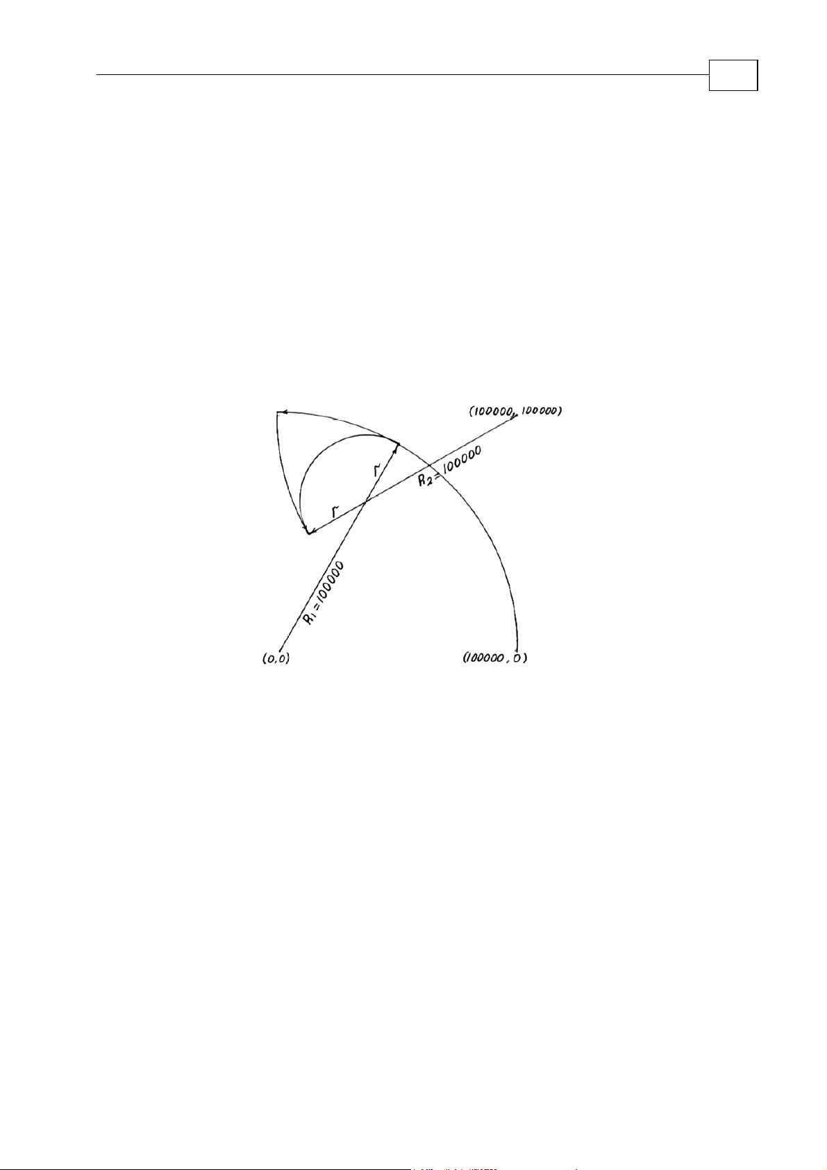
Motion Library Tutorial Switch Radius Calculation

MAN-MLT (Ver 2.0)

C1 = (X1 – Xc2)/R2 = -0.866025

C2 = (Y1 – Yc2)/R2 = -0.5

2-41

C3 = X

C

c1 – X1

= Yc1 – Y1 = -50000

4

= 2(C1C

6

= -13397.459622

+ C2C

3

+ R1) = 273205.080767

4

C7 = (C3)2 + (C4)2 – (R1)2 = –7320508075.6888

r = -C7/C6 = 26794.919242

The switch radius in use must be less this value.

Figure 2-36

Line

O1O

Another case when the line

Figure 2-37 line

arc

C

1

does not intersect at least one of the circle segments (Figure 2-37)

2

(Xc1, Yc1) – (Xc2, Yc2)

. Draw a line O

O1O

between the circle C1 center and its start point P

1P1

does not intersect at least one of the circle segments. In

2

connecting two circle centers does not intersect circle

1(X1,Y1

). Center

(Xo, Yo) of the switch arc with maximum radius must belong to this line. To define maximum

radius

(X1 – Xo)/(X1 – Xc1) = r/R

(Y1 – Yo)/(Y1 – Yc1) = r/R

(Xo – Xc2)2 + (Yo – Yc2)2 = (R2 – r)

r, use the same system as in previous cases:

(2.3.2-6)

1

(2.3.2-7)

1

2

(2.3.2-8)

Motion Library Tutorial Switch Radius Calculation

MAN-MLT (Ver 2.0)

2-42

This system is similar to (4.2) – (4.4) and comes to the same solution r = –C

Figure 2-37

C1 = (X1 – Xc2)/R1

7/C6

where

= (Y1 – Yc2)/R

C

2

C3 = X

(2.3.2--9)

C

= Yc2 – Y

4

C6 = 2(C1C

= (C3)2 + (C4)2 – (R2)

C

7

c2

– X

1

3

1

+ C2C

+ R2)

4

2

2.3.3 No circle intersects the internal area of the other

In case the circle C

of the circle

one circle is less than

C

goes outside circle C

2

, restrictions on the switch radius are still possible if a sweep angle of at least

2

90

o

.

and circle C

1

doesn’t come from the internal area

1

Motion Library Tutorial Switch Radius Calculation

MAN-MLT (Ver 2.0)

2-43

Consider the case that the sweep angle of the first circle is β

β

the second circle is

) and circle C

Y

c1

) and circle C

Y

c2

intersect the circle arc C

l

4.3. Note:

line L

2

If

l1 >l

the length of the line L

1

: l2 = ρ((X2,Y2),(X3,Y3)).

for the maximum switch radius r calculation, use the following system:

2

(Xo – X1)/(X1 – Xc1) = r/R

(2.3.3-1)

– Y1)/(Y1 – Yc1) = r/R

(Y

o

< 90. Draw a line L1 defined by two points: circle C

2

start point (X

1

end point. If line L

2

then the intersection point of two lines is point (X

1,

1

) and line L2 defined by circle C

1,Y1

does not intersect circle arc C

1

: l1 = ρ((X1,Y1),(X3,Y3)) and l

1

< 90 and the sweep angle of

1

center (X

1

center point (X

2

and line L

2

, Y3) – Figure

3

the length of the

2

c1

does not

2

c2

,

(2.3.3-2)

(Xo – Xc2)2 + (Yo –Yc2)2 = (R2 + r)

(2.3.3-3)

Equations (2.3.3-1)-(2.3.3-2) can be written in the following format

Xo = X1 + r(X1 – Xc1)/R1 = X1 + rC1 , C1 = (X1 – Xc1)/R

(2.3.3-4)

Yo = Y1 + r(Y1 – Yc1)/R1 = Y1 + rC2 , C2 = (Y1 – Yc1)/R

(2.3.3-5)

Substituting into (2.3.3-3), the results are:

(X1 + rC1 – Xc2 )2 + (Y1 + rC2 – Yc2)2 = (rC1 + C3)2 + (rC2 + C4)2 = (R2 + r)

(2.3.3-6)

1

2

where C

Simplifying (2.3.3-6), the results are:

= X1 – Xc2 C4 = Y1 – Y

3

c2

.

r2[1 – (C1)2 – (C2)2] + r[2R2 – 2C1C3 – 2C2C4] +[(R2)2 – (C3)2 – (C4)2] =

Motion Library Tutorial Switch Radius Calculation

MAN-MLT (Ver 2.0)

2-44

r2C5 + rC6 + C7 = 0 (2.3.3-7)

But

1 – (C1)2 – (C2)2 = 1 – (X

So for r the results are:

r = – C

Similarly in the case when

7/C6

(Xo – X2)/(X2 – Xc2) = r/R

(Y

– Y2)/(Y2 – Yc2) = r/R

o

– Xc1)2/(R1)2 – (Y1 – Yc1)2/(R1)2 = 0 (2.3.3-8)

1

l2 > l

use the following system:

1,

2

(2.3.3-9)

(2.3.3-10)

(2.3.3-11)

(Xo – Xc1)2 + (Yo –Yc1)2 = (R1 + r) (2.3.3-12)

Equations (2.3.3-1) - (2.3.3-2) can be written in the following format

Xo = X2 + r(X2 – Xc2)/R2 = X2 + rC1 , C1 = (X2 – Xc2)/R

Yo = Y2 + r(Y2 – Yc2)/R2 = Y2 + rC2 , C2 = (Y2 – Yc2)/R

And substituting into (2.3.3-3), the results are:

2

(2.3.3-13)

(2.3.3-14)

(X2 + rC1 – Xc1 )2 + (Y2 + rC2 – Yc1)2 = (rC1 + C3)2 + (rC2 + C4)2 = (R2 + r)

(2.3.3-15)

where C

Simplifying (2.3.3-15), the results are:

= X2 – Xc1 C4 = Y2 – Y

3

c1

.

r2[1 – (C1)2 – (C2)2] + r[2R2 – 2C1C3 – 2C2C4] +[(R2)2 – (C3)2 – (C4)2] =

2

r

C5 + rC6 + C7 = 0 (2.3.3-16)

2

But

1 – (C1)2 – (C2)2 = 1 – (X

– Xc2)2/(R2)2 – (Y2 – Yc2)2/(R2)2 = 0 (2.3.3-17)

2

Motion Library Tutorial Switch Radius Calculation

MAN-MLT (Ver 2.0)

So for r, the results are:

2-45

r = –C

If L

(X

7/C6

intersects circle arc C

1

).

1,Y1

use point (X

2,

1,Y1

). If L

intersects circle arc C

2

(2.3.3-18)

use point

1,

Figure 2-38

Maestro Software Manual

MAN-MLT(Ver. 2.0)

Appendix A: Projection of a point on a line defined by the end points

A-1

The line L is defined by its end points P

from some point point and the length of the perpendicular

a) X1 = X

Xpr = X

(Xo,Yo) on the line L and find coordinates (Xpr, Ypr) of the projection

2

1

1(X1,Y1

h.

) and P2(X2,Y

). Drop a perpendicular

2

Ypr = Yo h = |X

– X1|

o

b) Y X

= Y

2

= X

pr

1

o

Ypr = Y1 h= |Y

c) X1 ≠ X

Line equation

– Y1|

o

and Y

2

≠ Y

2

1

(X– X1)/(X2 – X1) = (Y – Y1)/(Y2 – Y1) (a1.1)

That can be transformed into

(Y – Y1)∆X = (X – X1)∆Y

or

Y = (Y1dX + X∆Y – X1∆Y)/∆X = Y1 + k(X – X1) (a1.2)

Where

An equation of the perpendicular dropped from (Xo,Yo) on L can be written in a form

k = ∆Y/∆X = (Y

– Y1)/(X2 – X1)

2

(Y - Yo) = (-1/k)(X – Xo) = q(X – Xo) (a1.3)

or

Y = Yo + q(X – X

Substituting (a1.4) into (a1.2) the results are

) (a1.4)

o

Yo + q(X – Xo) = Y1 + k(X – X1) (a1.5)

That produces for X coordinate

X = (Yo – Y1 + kX

– qXo)/(k – q) (a1.6)

1

Maestro Software Manual Setting up the Demo Case

MAN-MLT(Ver. 2.0)

Y is from (a1.4). Coordinates (X,Y) of the intersection point line L and perpendicular

A-2

are coordinates of projection point

Having got a projection point (X Euclidian distance

h = [(Xp – Xo)2 + (Yp – Yo)2]

(X

p,Yp

1/2

).

p,Yp

) we can calculate the perpendicular length h as

(a1.7)

Maestro Software Manual

MAN-MLT (Ver. 2.0)

Appendix B: Coefficients of the line standard equation for the line defined by the end points

B-1

If the line L is defined by its end points (X

coefficients

a) X1 ≠ X

The line equation can be written in a form

A,B,C for the three possible cases:

and Y

2

≠ Y

1

.

2

) and (X2,Y2) we can calculate the

1,Y1

(X – X1)/(X2 – X1) = (Y – Y1)/(Y2 – Y1) (a2.1)

or

(X – X1)/ ∆X = (Y – Y1)/∆Y (a2.2)

that can be transformed into

X∆Y – X1∆Y –Y∆X + Y1∆X = X∆Y –Y∆X +(Y1∆X - X1∆Y) = 0 (a2.3)

From (a2.3) we get

A = ∆Y, B = –∆X, C = Y1∆X – X1∆Y (a2.4)

b) X1 ≠ X2 and Y1 = Y

.

2

The line equation is

Y = Y

So for

or Y – Y

1

= 0 (a2.5)

1

A, B and C we have A = 0, B = 1, C = –Y1 (a2.6) c) X1 = X X = X

So for

A, B, C we have

A = 1, B = 0, C = – X

and Y

2

or X – X1 = 0 (a2.7)

1

≠ Y

1

The line equation is

.

2

(a2.8)

1

Maestro Software Manual

MAN-MLT (Ver. 2.0)

Appendix C: Intersection point of two lines defined by the end points

C-1

Line L1 is defined by its end points P

points

Note: ∆X

Calculation of the two lines intersection point (X,Y) depends on the each line position relative to coordinate axes. The following cases are possible.

P3(X3,Y3) and P4(X4,Y4).

= X2 – X1, ∆Y1 = Y2 – Y1, ∆X2 = X4 – X3, ∆Y2 = Y4 – Y3,

1

k

= ∆Y1/∆X1, q1 = ∆X1/∆Y1, k2 = ∆Y2/∆X2, q2 = ∆X2/∆Y

1

1(X1,Y1

a) X1 ≠ X2, Y1 ≠ Y2, X3 ≠ X4, Y3 ≠ Y

To define intersection point, use

(X – X1)∆Y1 = (Y – Y1)∆X

(X – X3)∆Y2 = (Y – Y3)∆X

1

2

) and P2(X2,Y2). Line L2 is defined by end

4

(a3.1)

(a3.2)

or

X∆Y1 – X1∆Y1 = Y∆X1 – Y1∆X

X∆Y2 – X3∆Y2 = Y∆X2 – Y3∆X

1

2

(a3.3)

(a3.4)

2

From (a3.3) the results are

X = X1 + Yq1 – Y1q

and substituting into (a3.4) the results are

(X1 + Yq1 – Y1q1)∆Y2 – X3∆Y

that produces

1

= Y∆X2 – Y3∆X

2

(a3.5)

(a3.6)

Y = [(q1Y1 + X3 – X1)∆Y2 –Y3∆X2]/(q1∆Y2 – ∆X2) (a3.7)

and X can be calculated by (a3.5).

b) X

≠ X2, Y1 ≠ Y2, X3 = X4, Y3 ≠ Y

1

To find an intersection point use

(X – X1)/∆X1 = (Y – Y1)/∆Y

1

(a3.8)

X = X

(a3.9)

3

4

Maestro Software Manual Performance Considerations

MAN-MLT (Ver. 2.0)

or

C-2

(X3 – X1)/∆X1 = (Y – Y1)/∆Y

1

(a3.10)

and finally for coordinate Y of intersection point the results are

Y = Y1 + k1(X3 – X1)

(a3.11)

c) X

≠ X2, Y1 ≠ Y2, X3 ≠ X4, Y3 = Y

1

To find an intersection point use

(X – X1)/∆X1 = (Y – Y1)/∆Y

Y = Y

That produces

3

1

4

(a3.12)

(a3.13)

X = X1 + q1(Y3 – Y1) (a3.14)

d) X

= X2, Y1 ≠ Y2, X3 ≠ X4, Y3 ≠ Y

1

Two lines equations:

4

X = X

(X – X

For coordinate Y of intersection point we have

(X1 – X3)/∆X2 = (Y – Y3)/∆Y

e) X

Two lines equations:

Y = Y

(X – X3)/∆X2 = (Y – Y3)/∆Y

For coordinate X of intersection point the results are

(X – X3)/∆X2 = (Y1 – Y3)/∆Y

f) X

1

)/∆X2 = (Y – Y3)/∆Y

3

≠ X2, Y1 = Y2, X3 ≠ X4, Y3 ≠ Y

1

= X2, Y1 ≠ Y2, X3 ≠ X4, Y3 =Y

1

X = X1, Y = Y

3

2

=> Y = Y3 + k2(X1 – X3) (a3.17)

2

4

2

=> X = X3 + q2(Y1 – Y3) (a3.18)

2

4

(a3.15)

(a3.16)

g) X

≠ X2, Y1 = Y2, X3 = X4, Y3 ≠Y

1

X = X3, Y = Y

1

4

Maestro Software Manual

MAN-MLT (Ver. 2.0)

Appendix D: Circle – line intersection

points

The line is defined by its end points (X1,Y1) and (X2,Y2). The circle is defined by its radius R and center coordinates (X the intersection points using

(X – X1)/(X2 – X1) = (Y – Y1)/(Y2 – Y1) (a4.1) (X – Xo)2 + (Y – Yo)2 = R

, Yo). Consider the general case X1 ≠ X2 and Y1 ≠ Y2. In this case, calculate

o

2

(a4.2)

D-1

Note that k = (Y the following form

Y = kX + (Y1 – kX1) = kX+ C

Substituting (a4.3) into (a4.2) results in

(X – Xo)2 + (kX + C1 – Yo)2 – R2 = 0

Simplifying (a4.4) results in the following equation

– Y1)/(X2 – X1) and C1 = Y1 – kX1 equation (a4.1) can be written in

2

1

(a4.3)

(a4.4)

C3X2 + C4X + C5 = 0 (a4.5)

where

C2 = C1 – Yo, C3 = 1 + k2,

= 2*(–Xo + kC2), C5 = (Xo)2 + (C2)2 – R

C

4

Note that d = (C

X1 = (–C4 + d X2 = (–C4 – d

Respective Y coordinates can be calculated by (a4.3) as

Y1 = kX1 + C Y2 = kX2 + C

2

)

– 4C3C

4

1/2

)/(2C3) (a4.6)

1/2

)/(2C3) (a4.7)

1

and for intersection point X coordinates the results are

5

2

(a4.8)

(a4.9)

Consider the case X

X = X

and substituting into (a4.2) the results are

1

(Y – Yo)2 = R2 – (X1 – Xo)

and for Y the results are

1=

2=

Y

+ [R2 – (X1 – Xo)2]

o

Y

– [R2 – (X1 – Xo)2]

o

Y Y

= X

1

. In this case line equation

2

1/2

(a4.11)

1/2

(a4.12)

(a4.10)

ElmoMC Multi-Axis Motion Controller User Manual

Specifications and Main Features

Frequently Asked Questions

User Manual

Notice

Contents

Chapter 1: General Description

1.1 Introduction

1.2 Vector properties

1.3 Trajectory generation

1.3.1 Line

1.3.2 Circle

1.3.3 Spline

1.3.3.1 Examples for the two-dimensional spline interpolation

1.3.3.2 Examples of three-dimensional spline interpolatio n

1.3.4 Polyline

1.3.4.1 Examples for the two-dimensional polyline

1.3.4.2 Examples for the three-dimensional polyline

1.4 Transition to a new trajectory with a non-zero velocity

Chapter 2: Switch Radius Calculation

2.1 Line – line intersection

2.2 Circle – line intersection

2.2.1 Line goes inside the circle

2.2.1.1 Switch arc center and circle center belong to two different half planes defined by the line L

2.2.1.2Switch arc center and a circle center belong to the same half plane.

2.2.1.3 Line intersects the center of the circle

2.2.2 Switch arc radius calculation by the distance from the intersection point

2.2.2.1 Initial circle center and switch arc center belong to the same half-plane

2.2.2.1.1 Line continues outside the circle (Figure 2-17)

2.2.2.1.2 Line continues inside the circle (Figure 2-18)

2.2.2.2 Initial circle center and switch arc center belong to two half planes defined by the line L.

2.2.2.2.1 Line continues outside the circle (Figure 2-19)

2.2.2.2.2 Line continues inside the circle (Figure 2-20)

2.2.2.3 Circle center (Xc,Yc) Є L1 (line L1 intersects the center of the circle)

2.2.2.3.1 Line goes outside of the circle (Figure 2.11).

2.2.2.3.2 Line goes inside the circle (Figure 2.12)

2.2.3 Line goes outside the circle

2.2.3.2 Line parallel to the circle arc init radius

2.3 Circle – circle intersection

2.3.1 One of two circle arcs intersects the internal area of the second

2.3.2 Each circle intersects the internal area of the second

2.3.3 No circle intersects the internal area of the other

Appendix A: Projection of a point on a line defined by the end points

Appendix B: Coefficients of the line standard equation for the line defined by the end points

Appendix C: Intersection point of two lines defined by the end points