Agilent Technologies 22ES, 8719ET, 22ET, 20ET, 20ES User Manual

Download

User’s Guide

Agilent Technologies

8719ET/20ET/22ET

8719ES/20ES/22ES

Network Analyzers

Part Number: 08720-90392

Printed in U SA

June 2002

Supersede s: February 2001

Notice

The information contained in this document is subject to change without notice. Agilent Technologies makes no warranty of any kind with regard to this material,

including but not limited to, the implied warranties of merchantability and fitness for a particular purpose. Agilent Technologies shall not be liable for errors contained herein or for incidental or consequent ial damages in connect ion with the furnishing , performance, or use of this material.

Certification

Agilent Technologie s certi f ies that this produc t m et i ts p ub lis hed speci fi c ations a t the time of shipment from the factory. Agilent Technologies further certifies that its calibration measurements are traceable to the United States National Institute of Standards and Technology, to the extent allowed by the Institute’s calibration facility, and to the calibration facilities of other International Standards Organization members.

Regulatory Inf ormation

The regulatory information is located in Chapter 8 , “Safety and Regulatory Information.”

Warranty

THE MATERIAL CONTAINED IN THIS DOCUMENT IS PROVIDED “ AS IS,” AND IS SUBJECT TO BEING CHANGED, WITHOUT NOTICE, IN FUTURE EDITIONS. FURTHER, TO THE MAXIMUM EXTENT PERMITTED BY APPLICABLE LAW, AGILENT DISCLAIMS ALL WARRANTIES, EITHER EXPRESS OR IMPLIED WITH REGARD TO THIS MANUAL AND ANY INFORMATION CONTAINED HEREIN, INCLUDING BUT NOT LIMITED TO THE IMPLIED WARRANTIES OF MERCHANTABILITY AND FITNESS FOR A PARTICULAR PURPOSE. AGILENT SHALL NOT BE LIABLE FOR ERRORS OR FOR INCIDENTAL OR CONSEQUENTIAL DAMAGES IN CONNECTION WITH THE FURNISHING, USE OR PERFORMANCE OF THIS DOCUMENT OR ANY INFORMATION CONTAINED HEREIN. SHOULD AGILENT AND THE USER HAVE A SEPARATE WRITTEN AGREEMENT WITH WARRANTY TERMS COVERING THE MATERIAL IN THIS DOCUMENT THAT CONFLICT WITH THESE TERMS, THE WARRANTY TERMS IN THE SEPARATE AGREEMENT WILL CONTROL.

Assistance

Product maintenance agreements and other customer assistance agreements are availa ble for Agilent Technologies products. For any assistance, contact your nearest Agilent Technologies sales or service office. See Table 8-1 for the nearest office.

Safety Note s

Front-Panel Key

SOFTKEY

The following safety notes are used throughout this manual. Familiarize your self with each of the notes and its meaning before operating this instrument. All pertinent safety notes for using this product are located in Chapter 8 , “Safety and Regulatory

Information.”

WARNING Warning denotes a hazard. It calls attention to a procedure which, if

not correctly performed or adhered to, could result in injury or loss of life. Do not proceed beyond a warning note until the indicated conditions are fully un derstood and met.

CAUTION Caution denotes a hazard. It calls attention to a procedure that, if not

correctly performed or adhered to , would result in damage to or destructi on of the instrument. Do not proceed beyond a caution sign until the indicated conditions are fully understood and met.

How to Use This Guide

This guide uses the following conventions:

This represents a key physically located on the

instrument.

This represents a “softkey,” a key whose label is

determined by the instrument’s firmware.

Screen Text This represents text displayed on the instrument’s screen.

iii

Documentation Map

The Installation an d Quick Start Guide pr ovides procedures for installing, configuring, and verifying the operation of the analyzer. It also will help you familiarize yourself with the basic operation of the analyzer.

The User’s Guide shows how to make measurements, explains commonly-used features, and tells you how to get the most perform ance from your ana ly z e r.

The Reference Guide provides re fere n ce inform at i on, su ch as specifications, menu maps, and key definitions.

The Programm er’s Guide provides general GPIB programming informat ion, a comm an d reference, and e xample pr og ra ms. T he Programmer’s Gui de contains a CD-ROM with example programs.

The CD-ROM provides the Installa tio n and Qu ick Start Guide , the User’s Guid e, the Referen ce Guide , and the Progra mmer’s Guid e in PDF format for v ie wing or p rin t ing from a PC.

The Service Guide pr ovides information on calibrating, troubleshooting, and servicing your analyzer . The Serv ic e Gu ide i s not part of a standard shipment and is available only as Option 0BW, or by ordering part number 08720-90397. A CD-ROM with the Service Guide in PDF format is included for viewing or printing from a PC.

1. Making Measurements

Using This Chapter . . . . . . . . . . . . . . . . . . . . . . . . . . . . . . . . . . . . . . . . . . . . . . . . . . . . . . . . . .1-2

More Instrument Functions Not Described in This Guide . . . . . . . . . . . . . . . . . . . . . . . . . . .1-3

Making a Basic Measurement. . . . . . . . . . . . . . . . . . . . . . . . . . . . . . . . . . . . . . . . . . . . . . . . . .1-4

Step 1. Connect the device under test and any required test equipment. . . . . . . . . . . . . .1-4

Step 2. Choose the measurement parameters. . . . . . . . . . . . . . . . . . . . . . . . . . . . . . . . . . . .1-4

Step 3. Perform and apply the appropriate error-correction. . . . . . . . . . . . . . . . . . . . . . . .1-5

Step 4. Measure the device under test. . . . . . . . . . . . . . . . . . . . . . . . . . . . . . . . . . . . . . . . . .1-5

Step 5. Output the measurement results. . . . . . . . . . . . . . . . . . . . . . . . . . . . . . . . . . . . . . .1-6

Measuring Magnitude and Insertion Phase Response . . . . . . . . . . . . . . . . . . . . . . . . . . . . . .1-7

Measuring the Magnitude Response . . . . . . . . . . . . . . . . . . . . . . . . . . . . . . . . . . . . . . . . . . .1-7

Measuring Insertion Phase Response . . . . . . . . . . . . . . . . . . . . . . . . . . . . . . . . . . . . . . . . . .1-8

Using Display Functions . . . . . . . . . . . . . . . . . . . . . . . . . . . . . . . . . . . . . . . . . . . . . . . . . . . . .1-10

Titling the Active Channel Display . . . . . . . . . . . . . . . . . . . . . . . . . . . . . . . . . . . . . . . . . . .1-11

Viewing Both Primary Measurement Channels . . . . . . . . . . . . . . . . . . . . . . . . . . . . . . . .1-12

Viewing Four Measurement Channels. . . . . . . . . . . . . . . . . . . . . . . . . . . . . . . . . . . . . . . . .1-14

Customizing the Four-Channel Display . . . . . . . . . . . . . . . . . . . . . . . . . . . . . . . . . . . . . . .1-17

Using Memory Traces and Memory Math Functions . . . . . . . . . . . . . . . . . . . . . . . . . . . .1-19

Blanking the Display . . . . . . . . . . . . . . . . . . . . . . . . . . . . . . . . . . . . . . . . . . . . . . . . . . . . . .1-21

Adjusting the Colors of the Display . . . . . . . . . . . . . . . . . . . . . . . . . . . . . . . . . . . . . . . . . .1-22

Using Markers . . . . . . . . . . . . . . . . . . . . . . . . . . . . . . . . . . . . . . . . . . . . . . . . . . . . . . . . . . . . .1 - 2 4

To Use Continuous and Discrete Markers . . . . . . . . . . . . . . . . . . . . . . . . . . . . . . . . . . . . .1-24

To Activate Display Markers . . . . . . . . . . . . . . . . . . . . . . . . . . . . . . . . . . . . . . . . . . . . . . . .1-25

To Move Marker Information Off the Grids . . . . . . . . . . . . . . . . . . . . . . . . . . . . . . . . . . . .1-26

To Use Delta (∆) Markers . . . . . . . . . . . . . . . . . . . . . . . . . . . . . . . . . . . . . . . . . . . . . . . . . .1-28

To Activate a Fixed Marker . . . . . . . . . . . . . . . . . . . . . . . . . . . . . . . . . . . . . . . . . . . . . . . . .1-29

To Couple and Un co u p le Display M a rkers . . . . . . . . . . . . . . . . . . . . . . . . . . . . . . . . . . . . .1- 3 1

To Use Polar Format Markers . . . . . . . . . . . . . . . . . . . . . . . . . . . . . . . . . . . . . . . . . . . . . . .1-32

To Use Smith Chart Markers . . . . . . . . . . . . . . . . . . . . . . . . . . . . . . . . . . . . . . . . . . . . . . .1-33

To Set Measurement Parameters Using Markers . . . . . . . . . . . . . . . . . . . . . . . . . . . . . . .1-34

Setting the CW Frequency . . . . . . . . . . . . . . . . . . . . . . . . . . . . . . . . . . . . . . . . . . . . . . . . . .1-38

To Search for a Specific Amplitude . . . . . . . . . . . . . . . . . . . . . . . . . . . . . . . . . . . . . . . . . . .1-39

To Calculate the Statistics of the Measurement Data . . . . . . . . . . . . . . . . . . . . . . . . . . . .1-42

Measuring Electrical Length and Phase Distortion . . . . . . . . . . . . . . . . . . . . . . . . . . . . . . .1-43

Measuring Electrical Length . . . . . . . . . . . . . . . . . . . . . . . . . . . . . . . . . . . . . . . . . . . . . . . .1-43

Measuring Phase Distortion . . . . . . . . . . . . . . . . . . . . . . . . . . . . . . . . . . . . . . . . . . . . . . . .1-45

Characterizing a Duplexer (ES Analyzers Only) . . . . . . . . . . . . . . . . . . . . . . . . . . . . . . . . . .1-49

Definitions. . . . . . . . . . . . . . . . . . . . . . . . . . . . . . . . . . . . . . . . . . . . . . . . . . . . . . . . . . . . . . .1-49

Procedure. . . . . . . . . . . . . . . . . . . . . . . . . . . . . . . . . . . . . . . . . . . . . . . . . . . . . . . . . . . . . . . .1-49

Measuring Amplifiers . . . . . . . . . . . . . . . . . . . . . . . . . . . . . . . . . . . . . . . . . . . . . . . . . . . . . . .1-52

Measuring Gain Compression . . . . . . . . . . . . . . . . . . . . . . . . . . . . . . . . . . . . . . . . . . . . . . .1-53

Measuring Gain and Rev erse Isolatio n Sim ultan eo usly (ES An alyze r s Only ) . . . . . . . . .1-57

Making High Power Measurements with Optio n 085 (ES Analyz ers On ly) . . . . . . . . . . .1-59

Making High Power Measurements with Optio n 012 (ES Analyz ers On ly) . . . . . . . . . . .1-65

Using the Swept List Mode to Test a Device . . . . . . . . . . . . . . . . . . . . . . . . . . . . . . . . . . . . .1-67

Connect the Device Under Test . . . . . . . . . . . . . . . . . . . . . . . . . . . . . . . . . . . . . . . . . . . . . .1-67

Observe the Characteristics of the Filter . . . . . . . . . . . . . . . . . . . . . . . . . . . . . . . . . . . . . .1-68

Choose the Measurement Parameters . . . . . . . . . . . . . . . . . . . . . . . . . . . . . . . . . . . . . . . .1-68

Calibrate and Measure . . . . . . . . . . . . . . . . . . . . . . . . . . . . . . . . . . . . . . . . . . . . . . . . . . . .1-70

Contents-v

Contents

Using Limit Lines to Test a Device. . . . . . . . . . . . . . . . . . . . . . . . . . . . . . . . . . . . . . . . . . . . .1-72

Setting Up the Measurement Parameters . . . . . . . . . . . . . . . . . . . . . . . . . . . . . . . . . . . . .1-72

Creating Flat Limit Lines . . . . . . . . . . . . . . . . . . . . . . . . . . . . . . . . . . . . . . . . . . . . . . . . . . 1-73

Creating a Sloping Limit Line . . . . . . . . . . . . . . . . . . . . . . . . . . . . . . . . . . . . . . . . . . . . . . 1-75

Creating Single Point Limits . . . . . . . . . . . . . . . . . . . . . . . . . . . . . . . . . . . . . . . . . . . . . . . 1-77

Editing Limit Segments . . . . . . . . . . . . . . . . . . . . . . . . . . . . . . . . . . . . . . . . . . . . . . . . . . .1-78

Running a Limit Test . . . . . . . . . . . . . . . . . . . . . . . . . . . . . . . . . . . . . . . . . . . . . . . . . . . . .1-79

Offsetting Limit Lines . . . . . . . . . . . . . . . . . . . . . . . . . . . . . . . . . . . . . . . . . . . . . . . . . . . . .1-79

Using Ripple Limits to Test a Device. . . . . . . . . . . . . . . . . . . . . . . . . . . . . . . . . . . . . . . . . . .1-81

Setting Up the List of Ripple Limits to Test. . . . . . . . . . . . . . . . . . . . . . . . . . . . . . . . . . . .1-81

Editing Ripple Test Limits. . . . . . . . . . . . . . . . . . . . . . . . . . . . . . . . . . . . . . . . . . . . . . . . . .1-84

Running the Ripple Test . . . . . . . . . . . . . . . . . . . . . . . . . . . . . . . . . . . . . . . . . . . . . . . . . . . 1-86

Using Bandwidth Limits to Test a Bandpass Filter . . . . . . . . . . . . . . . . . . . . . . . . . . . . . . . 1-92

Setting Up Bandwidth Limits . . . . . . . . . . . . . . . . . . . . . . . . . . . . . . . . . . . . . . . . . . . . . . .1-92

Running a Bandwidth Test . . . . . . . . . . . . . . . . . . . . . . . . . . . . . . . . . . . . . . . . . . . . . . . . . 1-94

Using Test Sequencing . . . . . . . . . . . . . . . . . . . . . . . . . . . . . . . . . . . . . . . . . . . . . . . . . . . . . .1-98

How to Use Test Sequencing . . . . . . . . . . . . . . . . . . . . . . . . . . . . . . . . . . . . . . . . . . . . . . . . 1-98

Creating a Sequence . . . . . . . . . . . . . . . . . . . . . . . . . . . . . . . . . . . . . . . . . . . . . . . . . . . . . .1-98

Running a Sequence . . . . . . . . . . . . . . . . . . . . . . . . . . . . . . . . . . . . . . . . . . . . . . . . . . . . . 1-100

Stopping a Sequence . . . . . . . . . . . . . . . . . . . . . . . . . . . . . . . . . . . . . . . . . . . . . . . . . . . . .1-100

Editing a Sequence . . . . . . . . . . . . . . . . . . . . . . . . . . . . . . . . . . . . . . . . . . . . . . . . . . . . . .1-100

Clearing a Sequence from Memory . . . . . . . . . . . . . . . . . . . . . . . . . . . . . . . . . . . . . . . . .1-102

Changing the Sequence Title . . . . . . . . . . . . . . . . . . . . . . . . . . . . . . . . . . . . . . . . . . . . . . 1-103

Naming Files Generated by a Sequence . . . . . . . . . . . . . . . . . . . . . . . . . . . . . . . . . . . . . 1-103

Storing a Sequence on a Disk . . . . . . . . . . . . . . . . . . . . . . . . . . . . . . . . . . . . . . . . . . . . . .1-104

Loading a Sequence from Disk . . . . . . . . . . . . . . . . . . . . . . . . . . . . . . . . . . . . . . . . . . . . . 1-104

Purging a Sequence from Disk . . . . . . . . . . . . . . . . . . . . . . . . . . . . . . . . . . . . . . . . . . . . .1-104

Printing a Sequence . . . . . . . . . . . . . . . . . . . . . . . . . . . . . . . . . . . . . . . . . . . . . . . . . . . . .1-105

In-Depth Sequencing Information . . . . . . . . . . . . . . . . . . . . . . . . . . . . . . . . . . . . . . . . . .1-105

Using Test Sequencing to Test a Device. . . . . . . . . . . . . . . . . . . . . . . . . . . . . . . . . . . . . . . . 1-114

Cascading Multiple Example Sequences . . . . . . . . . . . . . . . . . . . . . . . . . . . . . . . . . . . . .1-114

Loop Counter Example Sequence . . . . . . . . . . . . . . . . . . . . . . . . . . . . . . . . . . . . . . . . . . . 1-115

Generating Files in a Loop Counter Example Sequence . . . . . . . . . . . . . . . . . . . . . . . . . 1-116

Limit Test Example Sequence . . . . . . . . . . . . . . . . . . . . . . . . . . . . . . . . . . . . . . . . . . . . .1-118

2. Making Mixer Measurements (Option 089 Only)

Using This Chapter. . . . . . . . . . . . . . . . . . . . . . . . . . . . . . . . . . . . . . . . . . . . . . . . . . . . . . . . . . 2-2

Mixer Measure men t Ca pabilities . . . . . . . . . . . . . . . . . . . . . . . . . . . . . . . . . . . . . . . . . . . . . . . 2-3

Measurement Considerations . . . . . . . . . . . . . . . . . . . . . . . . . . . . . . . . . . . . . . . . . . . . . . . . . 2-4

Minimizing Source and Load Mismatches . . . . . . . . . . . . . . . . . . . . . . . . . . . . . . . . . . . . . . 2-4

Reducing the Effect of Spurious Responses . . . . . . . . . . . . . . . . . . . . . . . . . . . . . . . . . . . . .2-5

Eliminating Unwanted Mixing and Leakage Signals . . . . . . . . . . . . . . . . . . . . . . . . . . . . .2-6

How RF and IF Are Defined . . . . . . . . . . . . . . . . . . . . . . . . . . . . . . . . . . . . . . . . . . . . . . . . . 2-7

Frequency Offset Mode Operation . . . . . . . . . . . . . . . . . . . . . . . . . . . . . . . . . . . . . . . . . . . . 2-9

LO Frequency Accuracy and Stability . . . . . . . . . . . . . . . . . . . . . . . . . . . . . . . . . . . . . . . .2-10

Differences Between Internal and External R Channel Inputs . . . . . . . . . . . . . . . . . . . .2-10

Power Meter Calibration . . . . . . . . . . . . . . . . . . . . . . . . . . . . . . . . . . . . . . . . . . . . . . . . . . . 2-12

Conversion Loss Using the Frequency Offset Mode . . . . . . . . . . . . . . . . . . . . . . . . . . . . . . . 2-13

Sett i n g M easu rement Parameter s for the Pow e r M eter Ca libration . . . . . . . . . . . . . . . . 2-14

Contents-vi

Contents

Performing a Power Meter (Source) Calibration Over the RF Range . . . . . . . . . . . . . . . .2-15

Setting the Analyzer to Make an R Channel Measurement. . . . . . . . . . . . . . . . . . . . . . . .2-17

High Dynamic Range Swept RF/IF Conversion Loss . . . . . . . . . . . . . . . . . . . . . . . . . . . . . .2-20

Set Me a s urem e n t Par a mete rs for the I F Rang e . . . . . . . . . . . . . . . . . . . . . . . . . . . . . . . . .2- 2 0

Perform a Power Meter Calibration Over the IF Range. . . . . . . . . . . . . . . . . . . . . . . . . . .2-20

Perform a Receiver Calibration Over the IF Range . . . . . . . . . . . . . . . . . . . . . . . . . . . . . .2-22

Set the Analyzer to the RF Frequency Range. . . . . . . . . . . . . . . . . . . . . . . . . . . . . . . . . . .2-22

Perform a Power Meter Calibration Over the RF Range . . . . . . . . . . . . . . . . . . . . . . . . . .2-23

Perform t he Hi gh Dynami c R a nge Me a sure ment . . . . . . . . . . . . . . . . . . . . . . . . . . . . . . . . 2 - 2 4

Fixed IF Mixer Measurements . . . . . . . . . . . . . . . . . . . . . . . . . . . . . . . . . . . . . . . . . . . . . . . .2-27

Tuned Receiver Mode . . . . . . . . . . . . . . . . . . . . . . . . . . . . . . . . . . . . . . . . . . . . . . . . . . . . . .2-27

Sequence 1 Setup . . . . . . . . . . . . . . . . . . . . . . . . . . . . . . . . . . . . . . . . . . . . . . . . . . . . . . . . .2-27

Sequence 2 Setup . . . . . . . . . . . . . . . . . . . . . . . . . . . . . . . . . . . . . . . . . . . . . . . . . . . . . . . . .2-32

Phase or Group Delay Measurements . . . . . . . . . . . . . . . . . . . . . . . . . . . . . . . . . . . . . . . . . .2-35

Phase Measurements . . . . . . . . . . . . . . . . . . . . . . . . . . . . . . . . . . . . . . . . . . . . . . . . . . . . . .2-35

Phase Linearity and Group Delay . . . . . . . . . . . . . . . . . . . . . . . . . . . . . . . . . . . . . . . . . . . .2-35

Amplitude and Phase Tracking . . . . . . . . . . . . . . . . . . . . . . . . . . . . . . . . . . . . . . . . . . . . . . .2-39

Conversion Co m pres s i o n U s i ng the Frequ e n cy Off s e t M o de . . . . . . . . . . . . . . . . . . . . . . . .2- 4 0

Isolation Example Measurements . . . . . . . . . . . . . . . . . . . . . . . . . . . . . . . . . . . . . . . . . . . . .2-45

LO to RF Isolation . . . . . . . . . . . . . . . . . . . . . . . . . . . . . . . . . . . . . . . . . . . . . . . . . . . . . . . .2-45

RF Feedthrough . . . . . . . . . . . . . . . . . . . . . . . . . . . . . . . . . . . . . . . . . . . . . . . . . . . . . . . . . .2-47

SWR / Return Loss . . . . . . . . . . . . . . . . . . . . . . . . . . . . . . . . . . . . . . . . . . . . . . . . . . . . . . . .2-50

3. Making Time Domain Measurements

Using This Chapter . . . . . . . . . . . . . . . . . . . . . . . . . . . . . . . . . . . . . . . . . . . . . . . . . . . . . . . . . .3-2

Introduction to Time Domain Measurements . . . . . . . . . . . . . . . . . . . . . . . . . . . . . . . . . . . . .3-3

Making Transmission Response Measurements . . . . . . . . . . . . . . . . . . . . . . . . . . . . . . . . . . .3-5

Making Reflection Response Measurements . . . . . . . . . . . . . . . . . . . . . . . . . . . . . . . . . . . . . .3-9

Time Domain Bandpass Mode. . . . . . . . . . . . . . . . . . . . . . . . . . . . . . . . . . . . . . . . . . . . . . . . .3-12

Adjusting the Relative Velocity Factor . . . . . . . . . . . . . . . . . . . . . . . . . . . . . . . . . . . . . . . .3-12

Reflection Measurements Using Bandpass Mode . . . . . . . . . . . . . . . . . . . . . . . . . . . . . . .3-12

Transmission Measurements Using Bandpass Mode . . . . . . . . . . . . . . . . . . . . . . . . . . . .3-14

Time Domain Low Pass Mode . . . . . . . . . . . . . . . . . . . . . . . . . . . . . . . . . . . . . . . . . . . . . . . . .3-15

Setti ng the Frequenc y Ra nge fo r T i me Do m a in Low Pass . . . . . . . . . . . . . . . . . . . . . . . .3 - 1 5

Reflection Measurements in Time Domain Low Pa ss . . . . . . . . . . . . . . . . . . . . . . . . . . . .3-16

Fault Location Measurements Using Low Pass . . . . . . . . . . . . . . . . . . . . . . . . . . . . . . . . .3-18

Transmiss ion M easur emen t s in Tim e Dom a i n Low Pass . . . . . . . . . . . . . . . . . . . . . . . . . 3 - 1 9

Transforming CW Time Measurements into the Frequency Domain . . . . . . . . . . . . . . . . .3-22

Forward Transform Measurements . . . . . . . . . . . . . . . . . . . . . . . . . . . . . . . . . . . . . . . . . .3-22

Masking . . . . . . . . . . . . . . . . . . . . . . . . . . . . . . . . . . . . . . . . . . . . . . . . . . . . . . . . . . . . . . . . . .3-26

Windowing . . . . . . . . . . . . . . . . . . . . . . . . . . . . . . . . . . . . . . . . . . . . . . . . . . . . . . . . . . . . . . . .3-27

Range . . . . . . . . . . . . . . . . . . . . . . . . . . . . . . . . . . . . . . . . . . . . . . . . . . . . . . . . . . . . . . . . . . . .3 - 3 0

Resolution . . . . . . . . . . . . . . . . . . . . . . . . . . . . . . . . . . . . . . . . . . . . . . . . . . . . . . . . . . . . . . . .3-32

Response Resolution . . . . . . . . . . . . . . . . . . . . . . . . . . . . . . . . . . . . . . . . . . . . . . . . . . . . . .3-32

Range Resolution . . . . . . . . . . . . . . . . . . . . . . . . . . . . . . . . . . . . . . . . . . . . . . . . . . . . . . . . .3-34

Gating . . . . . . . . . . . . . . . . . . . . . . . . . . . . . . . . . . . . . . . . . . . . . . . . . . . . . . . . . . . . . . . . . . .3-35

Setting the Gate . . . . . . . . . . . . . . . . . . . . . . . . . . . . . . . . . . . . . . . . . . . . . . . . . . . . . . . . . .3-35

Selecting Gate Shape . . . . . . . . . . . . . . . . . . . . . . . . . . . . . . . . . . . . . . . . . . . . . . . . . . . . . .3-36

Contents-vii

Contents

4. Printing, Plotting, and Saving Mea sureme nt Resul ts

Using This Chapter. . . . . . . . . . . . . . . . . . . . . . . . . . . . . . . . . . . . . . . . . . . . . . . . . . . . . . . . . . 4-2

Printing or Plotting Your Measurement Results . . . . . . . . . . . . . . . . . . . . . . . . . . . . . . . . . .4-3

Configuring a Print Function . . . . . . . . . . . . . . . . . . . . . . . . . . . . . . . . . . . . . . . . . . . . . . . . . .4-4

Defining a Print Function . . . . . . . . . . . . . . . . . . . . . . . . . . . . . . . . . . . . . . . . . . . . . . . . . . . . 4-6

If You Are Using a Color Printer . . . . . . . . . . . . . . . . . . . . . . . . . . . . . . . . . . . . . . . . . . . . . 4-6

To Reset the Printing Parameters to Default Values . . . . . . . . . . . . . . . . . . . . . . . . . . . . .4-7

Printing One Measurement Per Page . . . . . . . . . . . . . . . . . . . . . . . . . . . . . . . . . . . . . . . . . . .4-8

Printing Multiple Measurements Per Page . . . . . . . . . . . . . . . . . . . . . . . . . . . . . . . . . . . . . . .4-9

Configuring a Plot Function . . . . . . . . . . . . . . . . . . . . . . . . . . . . . . . . . . . . . . . . . . . . . . . . . .4-10

If You Are Plotting to an HPGL/2 Compatible Printer . . . . . . . . . . . . . . . . . . . . . . . . . . . 4-10

If You Are Plotting to a Pen Plotter . . . . . . . . . . . . . . . . . . . . . . . . . . . . . . . . . . . . . . . . . .4-12

If You Are Plotting Measurement Results to a Disk Drive . . . . . . . . . . . . . . . . . . . . . . . .4-13

Defining a Plot Function . . . . . . . . . . . . . . . . . . . . . . . . . . . . . . . . . . . . . . . . . . . . . . . . . . . .4-15

Choosing Display Elements . . . . . . . . . . . . . . . . . . . . . . . . . . . . . . . . . . . . . . . . . . . . . . . . 4-15

Selecting Auto-Feed . . . . . . . . . . . . . . . . . . . . . . . . . . . . . . . . . . . . . . . . . . . . . . . . . . . . . . .4-15

Selecting Pen Numbers and Colors . . . . . . . . . . . . . . . . . . . . . . . . . . . . . . . . . . . . . . . . . .4-16

Selecting Line Types . . . . . . . . . . . . . . . . . . . . . . . . . . . . . . . . . . . . . . . . . . . . . . . . . . . . . .4-17

Choosing Scale . . . . . . . . . . . . . . . . . . . . . . . . . . . . . . . . . . . . . . . . . . . . . . . . . . . . . . . . . . . 4- 1 7

Choosing Plot Speed . . . . . . . . . . . . . . . . . . . . . . . . . . . . . . . . . . . . . . . . . . . . . . . . . . . . . .4-18

To Reset the Plotting Parameters to Default Values . . . . . . . . . . . . . . . . . . . . . . . . . . . . . 4-18

Plotting One Measurement Per Page Using a Pen Plotter . . . . . . . . . . . . . . . . . . . . . . . . . . 4-19

Plotting Multiple Measurements Per Page Using a Pen Plotter . . . . . . . . . . . . . . . . . . . . .4-20

If You Are Plotting to an HPGL Compatible Printer . . . . . . . . . . . . . . . . . . . . . . . . . . . .4-21

To View Plot Files on a PC . . . . . . . . . . . . . . . . . . . . . . . . . . . . . . . . . . . . . . . . . . . . . . . . . . .4-22

Using Ami Pro . . . . . . . . . . . . . . . . . . . . . . . . . . . . . . . . . . . . . . . . . . . . . . . . . . . . . . . . . . . 4- 2 3

Using Freelance . . . . . . . . . . . . . . . . . . . . . . . . . . . . . . . . . . . . . . . . . . . . . . . . . . . . . . . . . . 4-23

Converting HPGL Files for Use with Other PC Applications . . . . . . . . . . . . . . . . . . . . . . 4-24

Outputting Plot Files from a PC to a Plotter . . . . . . . . . . . . . . . . . . . . . . . . . . . . . . . . . . . .4-24

Outputting Plot Files from a PC to an HPGL Compatible Printer . . . . . . . . . . . . . . . . . . .4-25

Step 1. Store the HPGL initialization sequence. . . . . . . . . . . . . . . . . . . . . . . . . . . . . . . . .4-25

Step 2. Store the exit HPGL mode and form feed sequence. . . . . . . . . . . . . . . . . . . . . . . .4-26

Step 3. Send the HPGL initialization sequence to the printer. . . . . . . . . . . . . . . . . . . . .4-26

Step 4. Send the plot file to the printer. . . . . . . . . . . . . . . . . . . . . . . . . . . . . . . . . . . . . . . .4-26

Step 5 . Se nd the exit HPGL mode a n d f orm fee d sequ ence t o the printer. . . . . . . . . . . . 4- 2 6

Outputting Single Page Plots Using a Printer . . . . . . . . . . . . . . . . . . . . . . . . . . . . . . . . . . . 4-26

Outputting Multiple Plots to a Single Page Using a Printer . . . . . . . . . . . . . . . . . . . . . . . . 4-27

Plotting Multiple Measurements Per Page from Disk . . . . . . . . . . . . . . . . . . . . . . . . . . . . . 4-28

To Plot Multiple Measurements on a Full Page . . . . . . . . . . . . . . . . . . . . . . . . . . . . . . . .4-29

To Plot Measu remen t s in Page Q u a d rant s . . . . . . . . . . . . . . . . . . . . . . . . . . . . . . . . . . . . 4-3 0

Titling the Displayed Measurement. . . . . . . . . . . . . . . . . . . . . . . . . . . . . . . . . . . . . . . . . . . . 4-32

Configuring the Analyzer to Produce a Time Stamp . . . . . . . . . . . . . . . . . . . . . . . . . . . . . . 4-33

Aborting a Print or Plot Process . . . . . . . . . . . . . . . . . . . . . . . . . . . . . . . . . . . . . . . . . . . . . . 4-33

Printing or Plotting the List Values or Operating Parameters . . . . . . . . . . . . . . . . . . . . . .4-34

If You Want a Single Page of Values . . . . . . . . . . . . . . . . . . . . . . . . . . . . . . . . . . . . . . . . . . 4-34

If You Want the Entire List of Values . . . . . . . . . . . . . . . . . . . . . . . . . . . . . . . . . . . . . . . . 4-34

Solving Problems with Printing or Plotting . . . . . . . . . . . . . . . . . . . . . . . . . . . . . . . . . . . . . 4-35

Saving and Recalling I nst ru m ent State s . . . . . . . . . . . . . . . . . . . . . . . . . . . . . . . . . . . . . . .4-36

Places Where You Can Save . . . . . . . . . . . . . . . . . . . . . . . . . . . . . . . . . . . . . . . . . . . . . . . . 4-36

Contents-viii

Contents

What You Can Save to the Analyzer’s Internal Memory . . . . . . . . . . . . . . . . . . . . . . . . . .4-36

What You Can Save to a Floppy Disk . . . . . . . . . . . . . . . . . . . . . . . . . . . . . . . . . . . . . . . . .4-37

What You Can Save to a Computer . . . . . . . . . . . . . . . . . . . . . . . . . . . . . . . . . . . . . . . . . . .4-37

Saving an Instrument State . . . . . . . . . . . . . . . . . . . . . . . . . . . . . . . . . . . . . . . . . . . . . . . . . .4-38

Saving Measurement Results . . . . . . . . . . . . . . . . . . . . . . . . . . . . . . . . . . . . . . . . . . . . . . . . .4-39

ASCII Data Formats . . . . . . . . . . . . . . . . . . . . . . . . . . . . . . . . . . . . . . . . . . . . . . . . . . . . . .4-41

Saving in Textual (CSV) Form . . . . . . . . . . . . . . . . . . . . . . . . . . . . . . . . . . . . . . . . . . . . . . .4-44

Saving in Graphical (JPEG) Form . . . . . . . . . . . . . . . . . . . . . . . . . . . . . . . . . . . . . . . . . . . .4-46

Instrument State Files . . . . . . . . . . . . . . . . . . . . . . . . . . . . . . . . . . . . . . . . . . . . . . . . . . . . .4-47

Saving Time Gated Frequency Data . . . . . . . . . . . . . . . . . . . . . . . . . . . . . . . . . . . . . . . . . .4-49

Differences between Raw, Data, and Format Arrays . . . . . . . . . . . . . . . . . . . . . . . . . . . . .4-49

Re-Saving an Instrument State . . . . . . . . . . . . . . . . . . . . . . . . . . . . . . . . . . . . . . . . . . . . . . .4-51

Deleting a File . . . . . . . . . . . . . . . . . . . . . . . . . . . . . . . . . . . . . . . . . . . . . . . . . . . . . . . . . . . . .4-5 2

To Delete an Instrument State File . . . . . . . . . . . . . . . . . . . . . . . . . . . . . . . . . . . . . . . . . .4-52

To Delete all Files . . . . . . . . . . . . . . . . . . . . . . . . . . . . . . . . . . . . . . . . . . . . . . . . . . . . . . . . .4-52

Renaming a File . . . . . . . . . . . . . . . . . . . . . . . . . . . . . . . . . . . . . . . . . . . . . . . . . . . . . . . . . . .4-53

Recalling a File . . . . . . . . . . . . . . . . . . . . . . . . . . . . . . . . . . . . . . . . . . . . . . . . . . . . . . . . . . . .4-54

Formatting a Disk . . . . . . . . . . . . . . . . . . . . . . . . . . . . . . . . . . . . . . . . . . . . . . . . . . . . . . . . . .4-54

Solving Problems with Saving or Recalling Files . . . . . . . . . . . . . . . . . . . . . . . . . . . . . . . . .4-55

If You Are Using an External Disk Drive . . . . . . . . . . . . . . . . . . . . . . . . . . . . . . . . . . . . . .4-55

5. Optimizing Measurement Results

Using This Chapter . . . . . . . . . . . . . . . . . . . . . . . . . . . . . . . . . . . . . . . . . . . . . . . . . . . . . . . . . .5-2

Taking Care of Microwave Connectors . . . . . . . . . . . . . . . . . . . . . . . . . . . . . . . . . . . . . . . . . . .5-3

Increasing Measurement Accuracy . . . . . . . . . . . . . . . . . . . . . . . . . . . . . . . . . . . . . . . . . . . . .5-4

Interconnecting Cables . . . . . . . . . . . . . . . . . . . . . . . . . . . . . . . . . . . . . . . . . . . . . . . . . . . . .5-4

Improper Calibration Techniques . . . . . . . . . . . . . . . . . . . . . . . . . . . . . . . . . . . . . . . . . . . . .5-4

Sweeping Too Fast for Electrically Long Devices . . . . . . . . . . . . . . . . . . . . . . . . . . . . . . . . .5-4

Connector Rep eatability . . . . . . . . . . . . . . . . . . . . . . . . . . . . . . . . . . . . . . . . . . . . . . . . . . . .5-4

Temperature Drift . . . . . . . . . . . . . . . . . . . . . . . . . . . . . . . . . . . . . . . . . . . . . . . . . . . . . . . . .5-5

Frequency Drift . . . . . . . . . . . . . . . . . . . . . . . . . . . . . . . . . . . . . . . . . . . . . . . . . . . . . . . . . . .5-5

Performance Verification . . . . . . . . . . . . . . . . . . . . . . . . . . . . . . . . . . . . . . . . . . . . . . . . . . . .5-5

Reference Plane and Port Extensions . . . . . . . . . . . . . . . . . . . . . . . . . . . . . . . . . . . . . . . . . .5-5

Maintaining Test Port Output Power During Sweep Retrace . . . . . . . . . . . . . . . . . . . . . . . . .5-7

Making Accurate Measurements of Electrically Long Devices . . . . . . . . . . . . . . . . . . . . . . . .5-8

The Cause of Measurement Problems . . . . . . . . . . . . . . . . . . . . . . . . . . . . . . . . . . . . . . . . .5-8

To Improve Measurement Results . . . . . . . . . . . . . . . . . . . . . . . . . . . . . . . . . . . . . . . . . . . .5-8

Increasing Sweep Speed. . . . . . . . . . . . . . . . . . . . . . . . . . . . . . . . . . . . . . . . . . . . . . . . . . . . . .5-10

To Use Swept List Mode . . . . . . . . . . . . . . . . . . . . . . . . . . . . . . . . . . . . . . . . . . . . . . . . . . .5-10

To Decrease the Frequency Span . . . . . . . . . . . . . . . . . . . . . . . . . . . . . . . . . . . . . . . . . . . .5-11

To Set the Auto Sweep Time Mode . . . . . . . . . . . . . . . . . . . . . . . . . . . . . . . . . . . . . . . . . . .5-12

To Widen the System Bandwidth . . . . . . . . . . . . . . . . . . . . . . . . . . . . . . . . . . . . . . . . . . . .5-12

To Reduce the Averaging Factor . . . . . . . . . . . . . . . . . . . . . . . . . . . . . . . . . . . . . . . . . . . . .5-12

To Reduce the Number of Measurement Points . . . . . . . . . . . . . . . . . . . . . . . . . . . . . . . . .5-12

To Set the Sweep Type . . . . . . . . . . . . . . . . . . . . . . . . . . . . . . . . . . . . . . . . . . . . . . . . . . . . .5-12

To View a Single Me a sur em ent C h a nnel . . . . . . . . . . . . . . . . . . . . . . . . . . . . . . . . . . . . . .5- 1 3

To Activate Chop Sweep Mode . . . . . . . . . . . . . . . . . . . . . . . . . . . . . . . . . . . . . . . . . . . . . .5-13

To Use External Calibration . . . . . . . . . . . . . . . . . . . . . . . . . . . . . . . . . . . . . . . . . . . . . . . .5-13

To Use Fast 2-Port Calibration (ES Analyzers Only) . . . . . . . . . . . . . . . . . . . . . . . . . . . . .5-13

Contents-ix

Contents

Increasing Dynamic Range . . . . . . . . . . . . . . . . . . . . . . . . . . . . . . . . . . . . . . . . . . . . . . . . . .5-15

Increase the Test Port Input Power . . . . . . . . . . . . . . . . . . . . . . . . . . . . . . . . . . . . . . . . . . 5-15

Reduce the Receiver Noise Floor . . . . . . . . . . . . . . . . . . . . . . . . . . . . . . . . . . . . . . . . . . . . 5-15

Reduce the Receiver Crosstalk . . . . . . . . . . . . . . . . . . . . . . . . . . . . . . . . . . . . . . . . . . . . . . 5-15

Reducing Noise . . . . . . . . . . . . . . . . . . . . . . . . . . . . . . . . . . . . . . . . . . . . . . . . . . . . . . . . . . . . 5-1 6

To Activate Averaging . . . . . . . . . . . . . . . . . . . . . . . . . . . . . . . . . . . . . . . . . . . . . . . . . . . . .5-16

To Change System Bandwidth . . . . . . . . . . . . . . . . . . . . . . . . . . . . . . . . . . . . . . . . . . . . . .5-16

To Use Direct Sampler Access Configurations (Opt ion 012 On ly). . . . . . . . . . . . . . . . . . .5-17

Reducing Receiver Crosstalk . . . . . . . . . . . . . . . . . . . . . . . . . . . . . . . . . . . . . . . . . . . . . . . . .5-18

Reducing Recall Time . . . . . . . . . . . . . . . . . . . . . . . . . . . . . . . . . . . . . . . . . . . . . . . . . . . . . . .5 - 1 8

6. Calibrating for Increased Measurement Accuracy

How to Use This Chapter . . . . . . . . . . . . . . . . . . . . . . . . . . . . . . . . . . . . . . . . . . . . . . . . . . . . .6-2

Introduction. . . . . . . . . . . . . . . . . . . . . . . . . . . . . . . . . . . . . . . . . . . . . . . . . . . . . . . . . . . . . . . . 6-3

Calibration Considerations . . . . . . . . . . . . . . . . . . . . . . . . . . . . . . . . . . . . . . . . . . . . . . . . . . .6-4

Measurement Parameters . . . . . . . . . . . . . . . . . . . . . . . . . . . . . . . . . . . . . . . . . . . . . . . . . . . 6-4

Device Measurements . . . . . . . . . . . . . . . . . . . . . . . . . . . . . . . . . . . . . . . . . . . . . . . . . . . . . . 6-4

Clarifying Type-N Connector Sex . . . . . . . . . . . . . . . . . . . . . . . . . . . . . . . . . . . . . . . . . . . . . 6-4

Omitting Isolation Calibration . . . . . . . . . . . . . . . . . . . . . . . . . . . . . . . . . . . . . . . . . . . . . . .6-4

Saving Calibration Data . . . . . . . . . . . . . . . . . . . . . . . . . . . . . . . . . . . . . . . . . . . . . . . . . . . .6-5

Restarting a Calibration . . . . . . . . . . . . . . . . . . . . . . . . . . . . . . . . . . . . . . . . . . . . . . . . . . . .6-5

The Calibration Standards . . . . . . . . . . . . . . . . . . . . . . . . . . . . . . . . . . . . . . . . . . . . . . . . . .6-5

Frequency Response of Calibration Standards . . . . . . . . . . . . . . . . . . . . . . . . . . . . . . . . . . 6-6

Interpolated Error Correction . . . . . . . . . . . . . . . . . . . . . . . . . . . . . . . . . . . . . . . . . . . . . . . 6-8

Error-Correction Stimulus State . . . . . . . . . . . . . . . . . . . . . . . . . . . . . . . . . . . . . . . . . . . . .6-9

Procedures for Error Correcting Your Measurements . . . . . . . . . . . . . . . . . . . . . . . . . . . . .6-10

Types of Error Correction . . . . . . . . . . . . . . . . . . . . . . . . . . . . . . . . . . . . . . . . . . . . . . . . . .6-10

Frequency Response Error Corrections . . . . . . . . . . . . . . . . . . . . . . . . . . . . . . . . . . . . . . . . . 6-12

Response Error Correction for Reflection Measurements . . . . . . . . . . . . . . . . . . . . . . . . . 6-12

Resp o n se Error Correction for Tran smiss i o n M e a suremen ts . . . . . . . . . . . . . . . . . . . . . . 6-14

Receiver Calibration . . . . . . . . . . . . . . . . . . . . . . . . . . . . . . . . . . . . . . . . . . . . . . . . . . . . . .6-15

Frequency Res ponse and Isolation Error Corrections . . . . . . . . . . . . . . . . . . . . . . . . . . . . .6-17

Response and Isolation Error Correction for Transmission Measurements . . . . . . . . . .6-17

Response and Isolation Error Correction for Reflection Measurements . . . . . . . . . . . . .6-19

Enhanced Frequency Response Error Correction . . . . . . . . . . . . . . . . . . . . . . . . . . . . . . . . . 6-22

Enhanced Reflection Calibration. . . . . . . . . . . . . . . . . . . . . . . . . . . . . . . . . . . . . . . . . . . . .6-25

One-Port Reflection Error Correction . . . . . . . . . . . . . . . . . . . . . . . . . . . . . . . . . . . . . . . . . . 6-26

Full Two-Port Error Correction (ES Analyzers Only). . . . . . . . . . . . . . . . . . . . . . . . . . . . . .6-29

Power Meter Measurement Calibration . . . . . . . . . . . . . . . . . . . . . . . . . . . . . . . . . . . . . . . .6-33

Loss of Power Meter Calibration Data . . . . . . . . . . . . . . . . . . . . . . . . . . . . . . . . . . . . . . . . 6-33

Interpolation in Power Meter Calibration . . . . . . . . . . . . . . . . . . . . . . . . . . . . . . . . . . . . . 6-34

Entering the Power Sensor Calibration Data . . . . . . . . . . . . . . . . . . . . . . . . . . . . . . . . . .6-34

Compensating for Directional Coupler Response . . . . . . . . . . . . . . . . . . . . . . . . . . . . . . . 6-35

Using Sample-and-Sweep Correction Mode . . . . . . . . . . . . . . . . . . . . . . . . . . . . . . . . . . . .6-36

Using Continuous Correction Mode . . . . . . . . . . . . . . . . . . . . . . . . . . . . . . . . . . . . . . . . . .6-38

Calibrating for Noninsertable Devices . . . . . . . . . . . . . . . . . . . . . . . . . . . . . . . . . . . . . . . . . 6-40

Adapter Removal Calibration (ES Analyzers Only) . . . . . . . . . . . . . . . . . . . . . . . . . . . . . .6-41

Perform the 2-Port Error Corrections . . . . . . . . . . . . . . . . . . . . . . . . . . . . . . . . . . . . . . . .6-42

Verify the Results . . . . . . . . . . . . . . . . . . . . . . . . . . . . . . . . . . . . . . . . . . . . . . . . . . . . . . . . 6- 4 5

Contents-x

Contents

Matched Adapters . . . . . . . . . . . . . . . . . . . . . . . . . . . . . . . . . . . . . . . . . . . . . . . . . . . . . . . .6 -45

Modify the Cal Kit Thru Definition . . . . . . . . . . . . . . . . . . . . . . . . . . . . . . . . . . . . . . . . . . .6-46

Minimizing Error When Using Adapters . . . . . . . . . . . . . . . . . . . . . . . . . . . . . . . . . . . . . . . .6-47

Making Non-Coaxial Measurements. . . . . . . . . . . . . . . . . . . . . . . . . . . . . . . . . . . . . . . . . . . .6-48

Fixtures . . . . . . . . . . . . . . . . . . . . . . . . . . . . . . . . . . . . . . . . . . . . . . . . . . . . . . . . . . . . . . . . .6-4 8

Calibrating for Non-Coaxial Devices (ES Analyzers Only) . . . . . . . . . . . . . . . . . . . . . . . . . .6-50

TRL Error Correction . . . . . . . . . . . . . . . . . . . . . . . . . . . . . . . . . . . . . . . . . . . . . . . . . . . . . .6-50

LRM Error Correction . . . . . . . . . . . . . . . . . . . . . . . . . . . . . . . . . . . . . . . . . . . . . . . . . . . . . . .6-54

Create a User-Defined LRM Calibration Kit. . . . . . . . . . . . . . . . . . . . . . . . . . . . . . . . . . . .6-54

Perform the LRM Calibration . . . . . . . . . . . . . . . . . . . . . . . . . . . . . . . . . . . . . . . . . . . . . . .6-56

Calibrating Using Electronic Calibration (ECal) . . . . . . . . . . . . . . . . . . . . . . . . . . . . . . . . . .6-58

Set Up the Measurement . . . . . . . . . . . . . . . . . . . . . . . . . . . . . . . . . . . . . . . . . . . . . . . . . . .6-58

Connect the ECal Equipment . . . . . . . . . . . . . . . . . . . . . . . . . . . . . . . . . . . . . . . . . . . . . . . .6-59

Select the ECal Options . . . . . . . . . . . . . . . . . . . . . . . . . . . . . . . . . . . . . . . . . . . . . . . . . . . .6-60

Perform the Calibration . . . . . . . . . . . . . . . . . . . . . . . . . . . . . . . . . . . . . . . . . . . . . . . . . . . .6-62

Display the Module Information . . . . . . . . . . . . . . . . . . . . . . . . . . . . . . . . . . . . . . . . . . . . .6-64

Perform the Confidence Check. . . . . . . . . . . . . . . . . . . . . . . . . . . . . . . . . . . . . . . . . . . . . . .6-65

Investigating the Calibration Results Using the ECal Service Menu . . . . . . . . . . . . . . . .6-67

Adapter Removal Using ECal (ES Analyzers Only). . . . . . . . . . . . . . . . . . . . . . . . . . . . . . . .6-69

Perform the 2-Port Error Corrections . . . . . . . . . . . . . . . . . . . . . . . . . . . . . . . . . . . . . . . . .6-71

Determine the Electrical Delay . . . . . . . . . . . . . . . . . . . . . . . . . . . . . . . . . . . . . . . . . . . . . .6-73

Remove the Adapter . . . . . . . . . . . . . . . . . . . . . . . . . . . . . . . . . . . . . . . . . . . . . . . . . . . . . . .6-74

Verify the Results . . . . . . . . . . . . . . . . . . . . . . . . . . . . . . . . . . . . . . . . . . . . . . . . . . . . . . . . .6- 7 5

7. Operating Concepts

Using This Chapter . . . . . . . . . . . . . . . . . . . . . . . . . . . . . . . . . . . . . . . . . . . . . . . . . . . . . . . . . .7-2

Where to Find More Information. . . . . . . . . . . . . . . . . . . . . . . . . . . . . . . . . . . . . . . . . . . . . .7-2

System Operation . . . . . . . . . . . . . . . . . . . . . . . . . . . . . . . . . . . . . . . . . . . . . . . . . . . . . . . . . . .7-3

The Built-In Synthesized Source . . . . . . . . . . . . . . . . . . . . . . . . . . . . . . . . . . . . . . . . . . . . . .7-3

The Built-In Test Set . . . . . . . . . . . . . . . . . . . . . . . . . . . . . . . . . . . . . . . . . . . . . . . . . . . . . . .7-4

The Receiver Block . . . . . . . . . . . . . . . . . . . . . . . . . . . . . . . . . . . . . . . . . . . . . . . . . . . . . . . . .7-4

The Microprocessor . . . . . . . . . . . . . . . . . . . . . . . . . . . . . . . . . . . . . . . . . . . . . . . . . . . . . . . .7-4

Required Peripheral Equipment . . . . . . . . . . . . . . . . . . . . . . . . . . . . . . . . . . . . . . . . . . . . . .7-4

Processing . . . . . . . . . . . . . . . . . . . . . . . . . . . . . . . . . . . . . . . . . . . . . . . . . . . . . . . . . . . . . . . . .7 - 5

Processing Details . . . . . . . . . . . . . . . . . . . . . . . . . . . . . . . . . . . . . . . . . . . . . . . . . . . . . . . . .7-6

Output Power . . . . . . . . . . . . . . . . . . . . . . . . . . . . . . . . . . . . . . . . . . . . . . . . . . . . . . . . . . . . . . .7-9

Understanding the Power Ranges . . . . . . . . . . . . . . . . . . . . . . . . . . . . . . . . . . . . . . . . . . . . .7-9

Power Coupling Options . . . . . . . . . . . . . . . . . . . . . . . . . . . . . . . . . . . . . . . . . . . . . . . . . . .7-10

Sweep Time . . . . . . . . . . . . . . . . . . . . . . . . . . . . . . . . . . . . . . . . . . . . . . . . . . . . . . . . . . . . . . .7-11

Manual Sweep Time Mode . . . . . . . . . . . . . . . . . . . . . . . . . . . . . . . . . . . . . . . . . . . . . . . . .7-11

Auto Sweep Time Mode . . . . . . . . . . . . . . . . . . . . . . . . . . . . . . . . . . . . . . . . . . . . . . . . . . . .7-11

Minimum Sweep Time . . . . . . . . . . . . . . . . . . . . . . . . . . . . . . . . . . . . . . . . . . . . . . . . . . . . .7-11

Source Attenuator Switch Protection . . . . . . . . . . . . . . . . . . . . . . . . . . . . . . . . . . . . . . . . . . .7-13

Allowing Repetitive Switching of the Attenuator . . . . . . . . . . . . . . . . . . . . . . . . . . . . . . .7-13

Channel Stimulus Coupling . . . . . . . . . . . . . . . . . . . . . . . . . . . . . . . . . . . . . . . . . . . . . . . . . .7-14

Sweep Types . . . . . . . . . . . . . . . . . . . . . . . . . . . . . . . . . . . . . . . . . . . . . . . . . . . . . . . . . . . . . .7-15

Linear Frequency Sweep (Hz) . . . . . . . . . . . . . . . . . . . . . . . . . . . . . . . . . . . . . . . . . . . . . . .7-15

Logarithmic Frequency Sweep (Hz) . . . . . . . . . . . . . . . . . . . . . . . . . . . . . . . . . . . . . . . . . .7-15

Stepped List Frequency Sweep (Hz) . . . . . . . . . . . . . . . . . . . . . . . . . . . . . . . . . . . . . . . . . .7-15

Contents-xi

Contents

Swept List Frequency Sweep (Hz) . . . . . . . . . . . . . . . . . . . . . . . . . . . . . . . . . . . . . . . . . . . 7-17

Power Sweep (dBm) . . . . . . . . . . . . . . . . . . . . . . . . . . . . . . . . . . . . . . . . . . . . . . . . . . . . . . .7-19

CW Time Sweep (Seconds) . . . . . . . . . . . . . . . . . . . . . . . . . . . . . . . . . . . . . . . . . . . . . . . . .7-19

Selecting Sweep Modes . . . . . . . . . . . . . . . . . . . . . . . . . . . . . . . . . . . . . . . . . . . . . . . . . . . .7-19

S-Parameters . . . . . . . . . . . . . . . . . . . . . . . . . . . . . . . . . . . . . . . . . . . . . . . . . . . . . . . . . . . . . 7-20

Understanding S-Parameters . . . . . . . . . . . . . . . . . . . . . . . . . . . . . . . . . . . . . . . . . . . . . . . 7-20

The S-Parameter Menu . . . . . . . . . . . . . . . . . . . . . . . . . . . . . . . . . . . . . . . . . . . . . . . . . . . .7-22

Analyzer Display Formats. . . . . . . . . . . . . . . . . . . . . . . . . . . . . . . . . . . . . . . . . . . . . . . . . . . .7-24

Log Magnitude Format . . . . . . . . . . . . . . . . . . . . . . . . . . . . . . . . . . . . . . . . . . . . . . . . . . . . 7-24

Phase Format . . . . . . . . . . . . . . . . . . . . . . . . . . . . . . . . . . . . . . . . . . . . . . . . . . . . . . . . . . . . 7-2 4

Group Delay Format . . . . . . . . . . . . . . . . . . . . . . . . . . . . . . . . . . . . . . . . . . . . . . . . . . . . . . 7-25

Smith Chart Format . . . . . . . . . . . . . . . . . . . . . . . . . . . . . . . . . . . . . . . . . . . . . . . . . . . . . .7-26

Polar Format . . . . . . . . . . . . . . . . . . . . . . . . . . . . . . . . . . . . . . . . . . . . . . . . . . . . . . . . . . . . 7- 2 7

Linear Magnitude Format . . . . . . . . . . . . . . . . . . . . . . . . . . . . . . . . . . . . . . . . . . . . . . . . .7-27

SWR Format . . . . . . . . . . . . . . . . . . . . . . . . . . . . . . . . . . . . . . . . . . . . . . . . . . . . . . . . . . . . 7 - 2 8

Real Format . . . . . . . . . . . . . . . . . . . . . . . . . . . . . . . . . . . . . . . . . . . . . . . . . . . . . . . . . . . . . 7- 2 9

Imaginary Format . . . . . . . . . . . . . . . . . . . . . . . . . . . . . . . . . . . . . . . . . . . . . . . . . . . . . . . .7-29

Group Delay Principles . . . . . . . . . . . . . . . . . . . . . . . . . . . . . . . . . . . . . . . . . . . . . . . . . . . . 7-29

Electrical Delay . . . . . . . . . . . . . . . . . . . . . . . . . . . . . . . . . . . . . . . . . . . . . . . . . . . . . . . . . . . .7-33

Noise Reduction Techniques. . . . . . . . . . . . . . . . . . . . . . . . . . . . . . . . . . . . . . . . . . . . . . . . . .7-34

Averaging . . . . . . . . . . . . . . . . . . . . . . . . . . . . . . . . . . . . . . . . . . . . . . . . . . . . . . . . . . . . . . . 7-34

Smoothing . . . . . . . . . . . . . . . . . . . . . . . . . . . . . . . . . . . . . . . . . . . . . . . . . . . . . . . . . . . . . . 7-3 5

IF Bandwidth Reduction . . . . . . . . . . . . . . . . . . . . . . . . . . . . . . . . . . . . . . . . . . . . . . . . . . . 7-35

Measurement Calibration . . . . . . . . . . . . . . . . . . . . . . . . . . . . . . . . . . . . . . . . . . . . . . . . . . . 7-37

What Is Accuracy Enhancement? . . . . . . . . . . . . . . . . . . . . . . . . . . . . . . . . . . . . . . . . . . . .7-37

What Causes Measurement Errors? . . . . . . . . . . . . . . . . . . . . . . . . . . . . . . . . . . . . . . . . .7-38

Characterizing Microwave Systematic Errors . . . . . . . . . . . . . . . . . . . . . . . . . . . . . . . . . . 7-41

How Effective Is Accuracy Enhancement? . . . . . . . . . . . . . . . . . . . . . . . . . . . . . . . . . . . . . 7-51

Calibration Routines. . . . . . . . . . . . . . . . . . . . . . . . . . . . . . . . . . . . . . . . . . . . . . . . . . . . . . . .7 - 5 4

Response Calibration . . . . . . . . . . . . . . . . . . . . . . . . . . . . . . . . . . . . . . . . . . . . . . . . . . . . .7-54

Response and Isolation Calibration . . . . . . . . . . . . . . . . . . . . . . . . . . . . . . . . . . . . . . . . . . 7-54

Enhanced Response Calibration . . . . . . . . . . . . . . . . . . . . . . . . . . . . . . . . . . . . . . . . . . . . . 7-54

S11 and S22 One-Port Calibration . . . . . . . . . . . . . . . . . . . . . . . . . . . . . . . . . . . . . . . . . . .7-55

Full Two- Por t Calibration (ES M odels Only ) . . . . . . . . . . . . . . . . . . . . . . . . . . . . . . . . . . . 7-55

TRL*/LRM* Two-Port Calibration . . . . . . . . . . . . . . . . . . . . . . . . . . . . . . . . . . . . . . . . . . .7-55

E-CAL . . . . . . . . . . . . . . . . . . . . . . . . . . . . . . . . . . . . . . . . . . . . . . . . . . . . . . . . . . . . . . . . . . 7-56

Modifying Calibration Kits . . . . . . . . . . . . . . . . . . . . . . . . . . . . . . . . . . . . . . . . . . . . . . . . . .7-57

Definitions . . . . . . . . . . . . . . . . . . . . . . . . . . . . . . . . . . . . . . . . . . . . . . . . . . . . . . . . . . . . . . 7-57

Procedure . . . . . . . . . . . . . . . . . . . . . . . . . . . . . . . . . . . . . . . . . . . . . . . . . . . . . . . . . . . . . . . 7-58

Modify Calibration Kit Menu . . . . . . . . . . . . . . . . . . . . . . . . . . . . . . . . . . . . . . . . . . . . . . .7-58

Verify Performance . . . . . . . . . . . . . . . . . . . . . . . . . . . . . . . . . . . . . . . . . . . . . . . . . . . . . . .7-65

Saving Modified Calibration Kits to a Disk . . . . . . . . . . . . . . . . . . . . . . . . . . . . . . . . . . . . 7-65

Modifying and Saving a Ca libr atio n Kit from the Calibrat io n Kit Se lection Menu. . . . . 7-66

TRL*/LRM* Calibration (ES Models Only) . . . . . . . . . . . . . . . . . . . . . . . . . . . . . . . . . . . . . .7-67

Why Use TRL Calibration? . . . . . . . . . . . . . . . . . . . . . . . . . . . . . . . . . . . . . . . . . . . . . . . . .7-67

TRL Terminology . . . . . . . . . . . . . . . . . . . . . . . . . . . . . . . . . . . . . . . . . . . . . . . . . . . . . . . . .7-68

How TRL*/LRM* Calibration Works . . . . . . . . . . . . . . . . . . . . . . . . . . . . . . . . . . . . . . . . .7-68

Improving Raw Source Match and Load Match for TRL*/LRM* Calibration . . . . . . . . . 7-71

How True TRL/LRM Works (Option 400 Only) . . . . . . . . . . . . . . . . . . . . . . . . . . . . . . . . .7-72

Contents-xii

Contents

The TRL Calibration Procedure . . . . . . . . . . . . . . . . . . . . . . . . . . . . . . . . . . . . . . . . . . . . .7-72

GPIB Operation . . . . . . . . . . . . . . . . . . . . . . . . . . . . . . . . . . . . . . . . . . . . . . . . . . . . . . . . . . . .7-78

Local Key . . . . . . . . . . . . . . . . . . . . . . . . . . . . . . . . . . . . . . . . . . . . . . . . . . . . . . . . . . . . . . .7-78

GPIB STATUS Indicators . . . . . . . . . . . . . . . . . . . . . . . . . . . . . . . . . . . . . . . . . . . . . . . . . .7-79

System Controller Mode . . . . . . . . . . . . . . . . . . . . . . . . . . . . . . . . . . . . . . . . . . . . . . . . . . .7-79

Talker/Listener Mode . . . . . . . . . . . . . . . . . . . . . . . . . . . . . . . . . . . . . . . . . . . . . . . . . . . . . .7-79

Pass Control Mode . . . . . . . . . . . . . . . . . . . . . . . . . . . . . . . . . . . . . . . . . . . . . . . . . . . . . . . .7-7 9

Address Menu . . . . . . . . . . . . . . . . . . . . . . . . . . . . . . . . . . . . . . . . . . . . . . . . . . . . . . . . . . . .7 -80

Using the Parallel Port . . . . . . . . . . . . . . . . . . . . . . . . . . . . . . . . . . . . . . . . . . . . . . . . . . . .7-80

Limit Line Operation. . . . . . . . . . . . . . . . . . . . . . . . . . . . . . . . . . . . . . . . . . . . . . . . . . . . . . . .7-82

Edit Limits Menu . . . . . . . . . . . . . . . . . . . . . . . . . . . . . . . . . . . . . . . . . . . . . . . . . . . . . . . . .7-83

Edit Segment Menu . . . . . . . . . . . . . . . . . . . . . . . . . . . . . . . . . . . . . . . . . . . . . . . . . . . . . . .7-83

Offset Limits Menu . . . . . . . . . . . . . . . . . . . . . . . . . . . . . . . . . . . . . . . . . . . . . . . . . . . . . . .7-8 3

Knowing the Instrument Modes . . . . . . . . . . . . . . . . . . . . . . . . . . . . . . . . . . . . . . . . . . . . . . .7-84

Network Analyzer Mode . . . . . . . . . . . . . . . . . . . . . . . . . . . . . . . . . . . . . . . . . . . . . . . . . . .7-84

Tuned Receiver Mode . . . . . . . . . . . . . . . . . . . . . . . . . . . . . . . . . . . . . . . . . . . . . . . . . . . . . .7-84

Frequency Offset Operation (Op tion 089) . . . . . . . . . . . . . . . . . . . . . . . . . . . . . . . . . . . . . .7-85

8. Sa fety and Regu latory Inf ormation

General Information. . . . . . . . . . . . . . . . . . . . . . . . . . . . . . . . . . . . . . . . . . . . . . . . . . . . . . . . . .8-2

Maintenance . . . . . . . . . . . . . . . . . . . . . . . . . . . . . . . . . . . . . . . . . . . . . . . . . . . . . . . . . . . . . .8-2

Assistance . . . . . . . . . . . . . . . . . . . . . . . . . . . . . . . . . . . . . . . . . . . . . . . . . . . . . . . . . . . . . . . .8-2

Shipment for Service . . . . . . . . . . . . . . . . . . . . . . . . . . . . . . . . . . . . . . . . . . . . . . . . . . . . . . .8-2

Safety Symbols . . . . . . . . . . . . . . . . . . . . . . . . . . . . . . . . . . . . . . . . . . . . . . . . . . . . . . . . . . . . .8-4

Instrument Markings . . . . . . . . . . . . . . . . . . . . . . . . . . . . . . . . . . . . . . . . . . . . . . . . . . . . . . . .8-4

Safety Considerations . . . . . . . . . . . . . . . . . . . . . . . . . . . . . . . . . . . . . . . . . . . . . . . . . . . . . . . .8-5

Safety Earth Ground . . . . . . . . . . . . . . . . . . . . . . . . . . . . . . . . . . . . . . . . . . . . . . . . . . . . . . .8-5

Before Applying Power . . . . . . . . . . . . . . . . . . . . . . . . . . . . . . . . . . . . . . . . . . . . . . . . . . . . . .8- 5

Servicing . . . . . . . . . . . . . . . . . . . . . . . . . . . . . . . . . . . . . . . . . . . . . . . . . . . . . . . . . . . . . . . . .8-6

General . . . . . . . . . . . . . . . . . . . . . . . . . . . . . . . . . . . . . . . . . . . . . . . . . . . . . . . . . . . . . . . . . .8-7

Compliance with German FTZ Emissions Requirements . . . . . . . . . . . . . . . . . . . . . . . . . .8-8

Compliance with German Noise Requirements . . . . . . . . . . . . . . . . . . . . . . . . . . . . . . . . . .8-8

Compliance with Canadian EMC Requirements . . . . . . . . . . . . . . . . . . . . . . . . . . . . . . . . .8-8

Declaration of Conformity . . . . . . . . . . . . . . . . . . . . . . . . . . . . . . . . . . . . . . . . . . . . . . . . . . . . .8-9

Contents-xiii

Contents

Contents-xiv

1 Making Measurements

1-1

Making Measurements

Using This Chapter

This chapter contains the following example procedures for making measurements. Mixer and time domain measurements are covered in Chapter 2 , "Making Mixer Measurements

(Option 089 Only) " and Chapter 3 , “Making Time Domain Measurements.” This chapter

also describes how to use most display, marker, and sequencing functions.

• "Making a Basic Measurement" on page 1-4

• "Measuring Magnitude and Insertion Phase Response" on page 1-7

• "Measuring Electrical Length and Phase Distortion" on page 1-43 — Electr ical Length

— Phase Distortion (deviation from linear phase, group delay)

• Characterizing a Duplexer (ES Analyzers Only)

• "Measuring Amplifiers" on page 1-52 — Measuring Gain Compression

— Measuring Gain Compression and Reverse Isolation Simultaneously

(ES Analyzers Only)

— Making High Power Measurements (ES Analyzers Only)

• "Using the Swept List Mode to Test a Device" on page 1-67

• "Using Limit Lines to Test a Device" on page 1-72

• "Using Test Sequencing to Test a Device" on page 1-114

The following chapters describe how to use more instrument functions (as indicated by their chapter titles):

• Chapter 4 , "Printing, Plotting, and Saving Measurement Results"

• Chapter 5 , "Optimizing Measurement Results"

• Chapter 6 , "Calibrating for Increased Measurement Accuracy"

1-2

Making Measurements

More Instrument Functions Not Described in This Guide

To learn about instrument functions not covered in this user’s guide, refer to the following chapters in the reference guide.

“Menu Maps” contains maps of the instrument menu structure. “Hardkey/Softkey Reference” contains descriptions of all instrument functions.

1-3

Making Measurements

PRESET : FACTORY

Making a Basic Measurement

There are five basic steps when you are making a measurement.

1. Connect the device under test and any required test equipment.

CAUTION Damage may result to the device under test (DUT) if it is sensitive to the

analyzer’s default output power lev el. To avoid damaging a sensitive DUT, be sure to lower the output power before connecting the DUT to the analyzer.

2. Choose the measurement parameters.

3. Perform and apply the appropriate error-correction.

4. Measure the device under test (DUT).

5. Output the measurement results.

This example procedure shows you how to measure the transmission response of a bandpass filt e r.

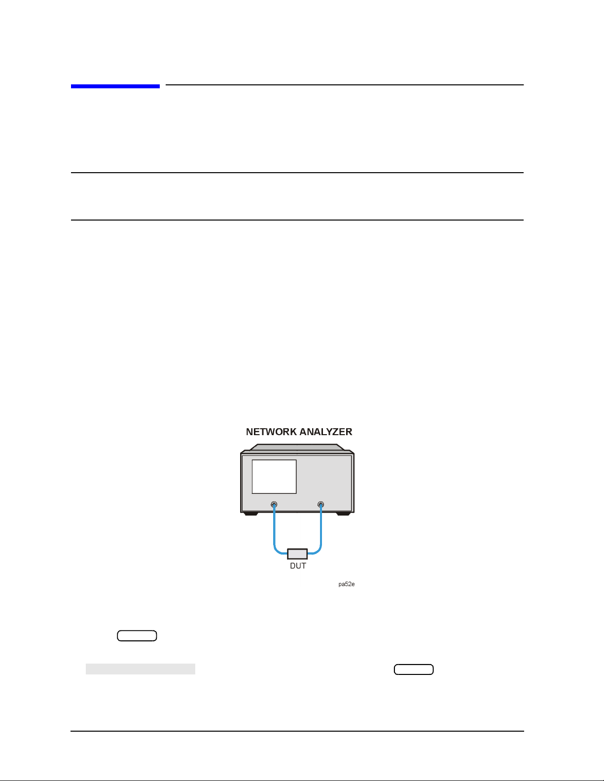
Step 1. Connect the device under test and any required test equipment.

Make the connections as shown in Figure 1-1.

Figure 1-1 Basic Measurement Setup

Step 2. Choose the measurement parameters.

Press .

Preset

To set preset the analyzer to the “Factory Preset” conditions, press the

1-4

softkey if it is not selected. Then press .

Preset

Setting the Frequency Range

POWER RANGE MAN

POWER RANGES

Sweep Setup

NUMBER OF POINTS

Trans: FWD S21 (B/R)

TRANSMISSN

AUTOSCALE

SELECT DISK

INTERNAL MEMORY

RETURN

SAVE STATE

Marker Search

SEARCH: MAX

To se t the center frequency to 134 MHz, press:

Making Measurements

Making a Basic Measurement

Center 134 M/µ

To set the span to 30 MHz, press:

Span 30 M/µ

NOTE You could also press the and keys and enter the frequency

Start Stop

range limits as start frequency and stop frequency values.

Setting the Source Power

To change the power level to −5 dBm, press:

Power −5 x1

NOTE You could a lso pres s and select

one of the power ranges to keep the power setting within the defined range.

Setting the Measurement

To change the number of measurement data points to 101, press:

To select the transmission measurement, press:

Meas

or on ET models:

To view the data trace, press:

Scale Ref

Step 3. Perform and apply the appropriate error-correction.

Refer to the Chapter 5 , “Optimizing Measurement Results,” for procedures on

correcting measurement errors. To save the instrument state and error- correction in the analyzer internal memory,

press:

Save/Recall

Step 4. Measure the device under test.

Replace any standard used for error-correction with the device under test. To measure the insertion loss of the bandpass filter, press:

1-5

Making Measurements

PRINT MONOCHROME

PLOT

Making a Basic Measurement

Step 5. Output the measurement results.

To create a printed copy of the measurement results, press:

(or )

Copy

Refer to Chapter 4 , “Printing, Plotting, and Saving Measurement Results ,” for

procedures on how to set up a printer and define a print, plot, or save results.

1-6

Making Measurements

Trans:FWD S21 (B/R)

TRANSMISSN

AUTO SCALE

Trans:FWD S21 (B/R)

TRANSMISSN

AUTO SCALE

CALIBRATE MENU

RESPONSE

THRU

Measuring Magnitude and Insertion Phase Response

Measuring Magnitud e and Insertion Phase Response

This measurement example shows you how to measure the maximum amplitude of a surface acoustic wave (SAW) filter and then how to view the measurement data in the phase format, which provides information about the phase response.

Measuring the Magnitude Response

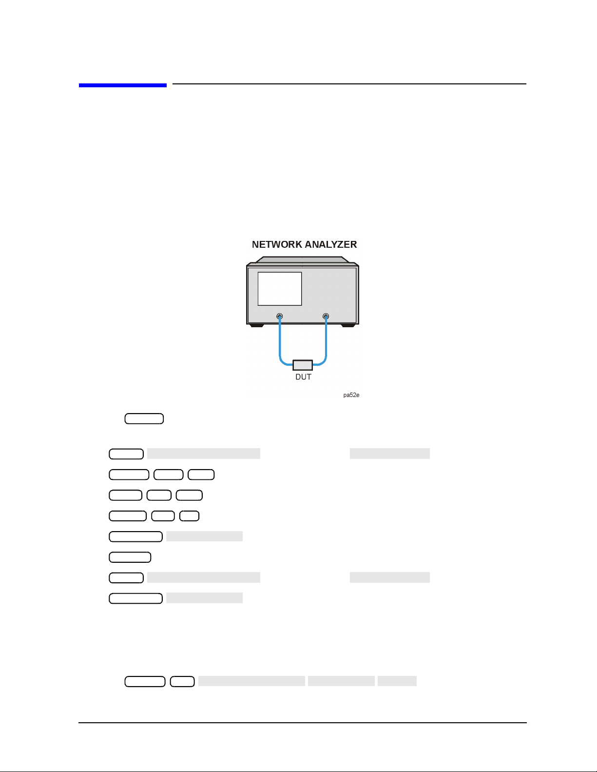
1. Connect your test device as shown in Figure 1-2.

Figure 1-2 Device Connections for Measuring a Magnitude Response

2. Press and choose the measurement settings. For this example the

Preset

measurement parameters are set as follows:

Meas Center 134 M/µ Span 50 M/µ Power −3 x1 Scale Ref Chan 2 Meas Scale Ref

or on ET models:

You may also want to select settings for the number of data points, averaging, and IF bandwidth.

3. Remove the device and connect the power cables together (thru) and perfo rm a response calibration using the following key presses.

Press .

Chan 1 Cal

1-7

Making Measurements

AUTO SCALE

Marker Search

SEARCH: MAX

DUAL | QUAD SETUP

DUAL CHAN ON

PHASE

Measuring Magnitude and Insertion Phase Response

If the channels are coupled (the default condition), this calibration is valid for both channels.

4. Reconnect your test device.

5. To better view the measurement trace, press:

Scale Ref

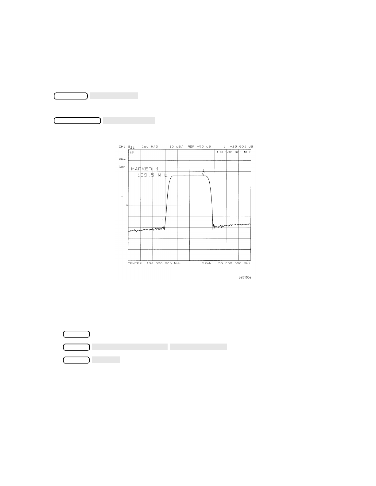
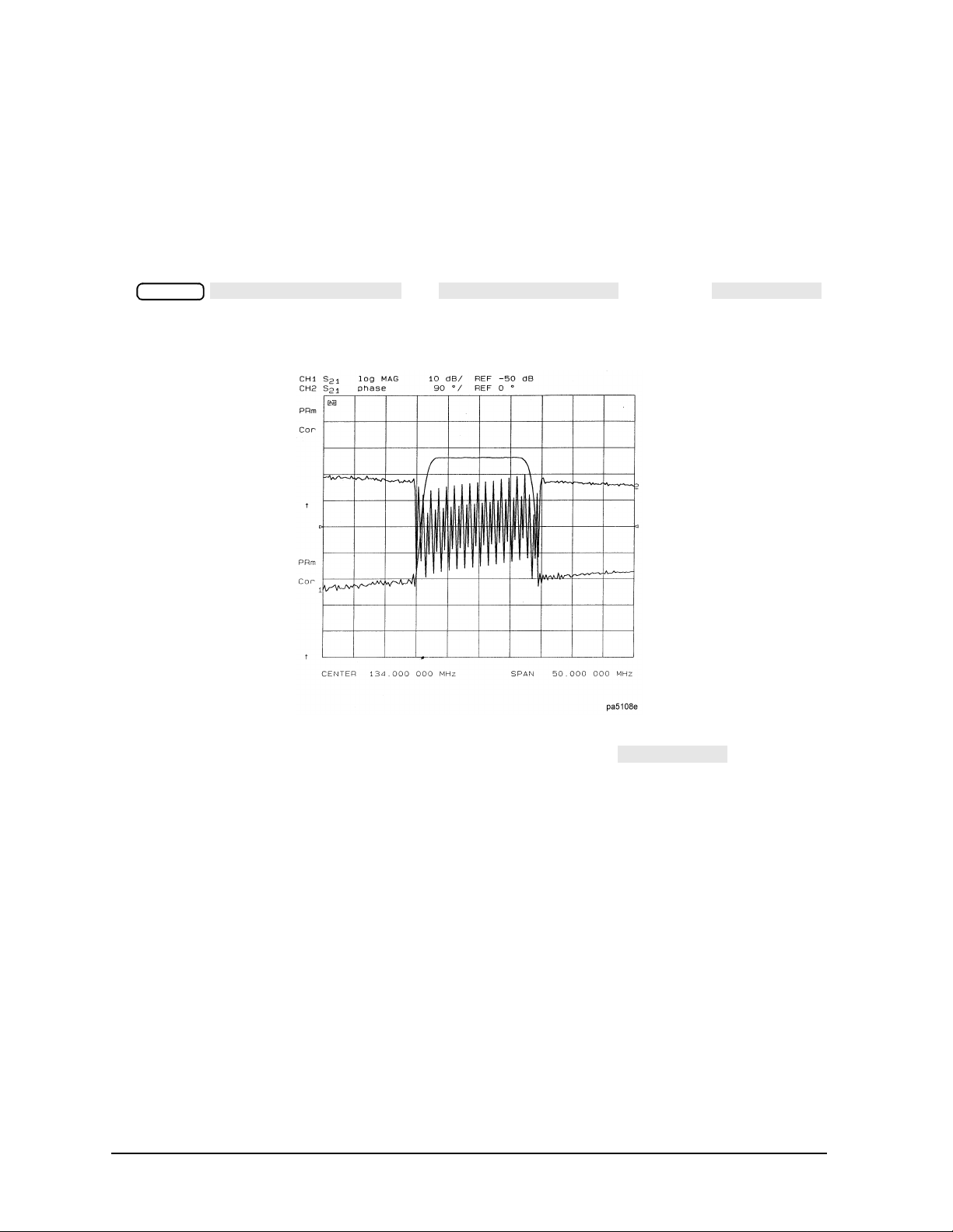
6. To locat e the maximum amplitude of the device resp onse, as shown in Figure 1-3 , p r ess :

Figure 1-3 Example Magnitude Response Measurement Results

Measuring Insertion Phase Response

7. To view both the magnitude and phase response of the device, as shown in Figure 1-4, press:

Chan 2 Display Format

The channel 2 portion of Figure 1-4 shows the insertion phase response of the device under test. The ana lyz er measures and displays phas e over the range o f −180° to +180°. As phase changes beyond these values, a sharp 360° transition occurs in the displayed data.

1-8

Measuring Magnitude and Insertion Phase Response

Figure 1-4 Example Insertion Phase Response Measurement

Making Measurements

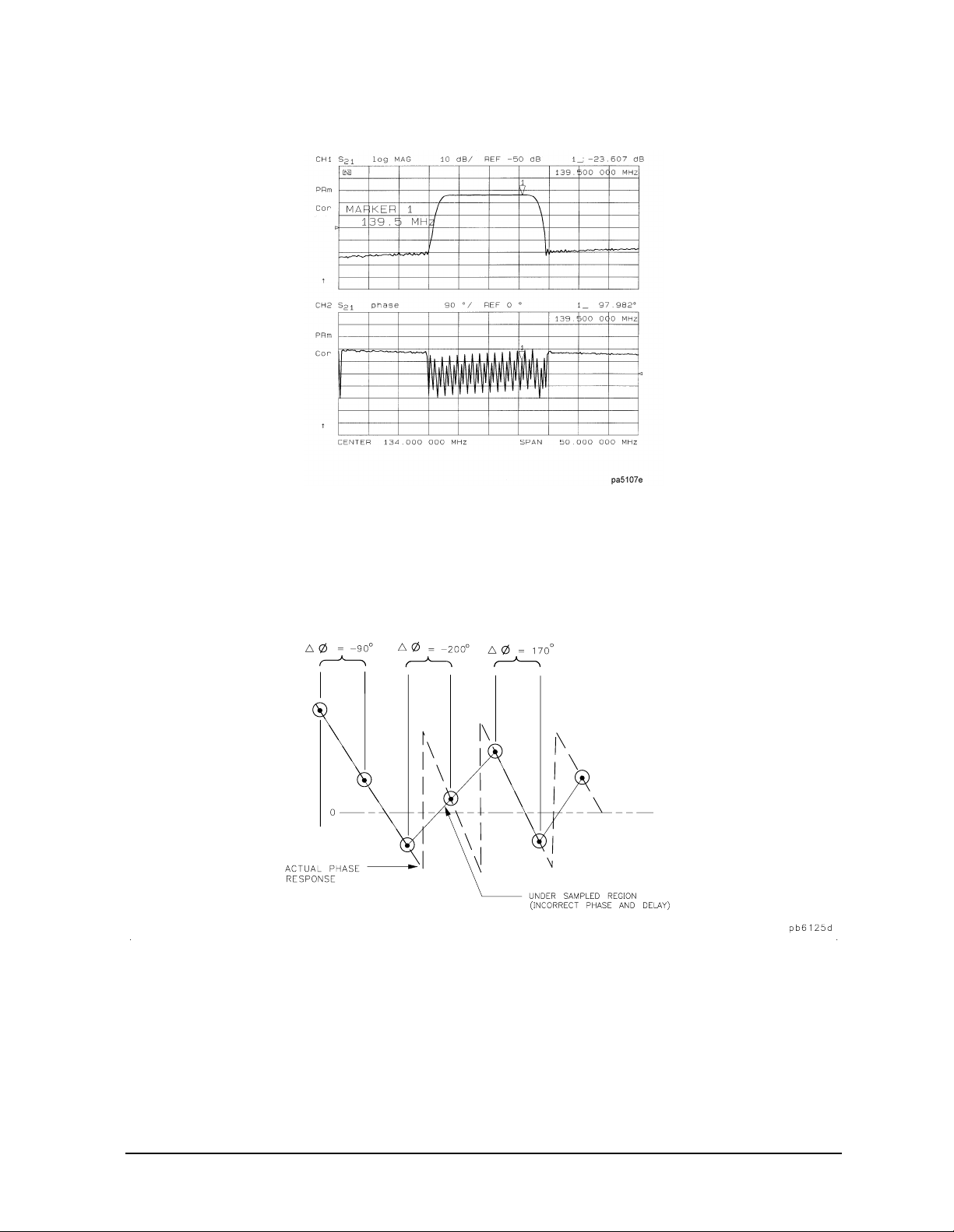
The phase response shown in Figure 1-5 is undersampled; that is, there is more than 180° phase delay between frequency points. If the ∆Φ ≥ 180°, incorrect phase and delay inform at io n may result . Figu re 1-5 shows an example of phase samples being with ∆Φ less than 180° and greater than 180°.

Figure 1 -5 Phase Samples

Undersampling may arise when measuring devices with long electrical length. To correct this problem, the frequency span should be reduced, or the number of points increased until ∆Φ is less than 180° per point. Electrical delay may also be used to compensate for this effect (as shown in the next example procedure).

1-9

Making Measurements

Using Display Functions

This section provides the necessary information for using the display functions. These functions are very helpful for displaying measurement data so that it will be easy to read. This section covers the following topics:

• Adding titles to your measurements

• Viewing both primary channels at the same time

• Viewing and customizing four-channel measurements

• Using the memory traces

• Using the memory math functions

• Blanking the analyzer’s display

• Changing the colors of the display

1-10

Titling the Active Channel Display

TITLE

ERASE TITLE

ENTER

SELECT LETTER

DONE

NEWLINE

FORMFEED

Making Measurements

Using Display Functions

1. Press to access the title menu.

Display

2. Press and enter the title you want for your measurement display.

• If you have a DIN keyboard attached to the analyzer, type the titl e you w ant from the keyboard. Then press to enter the title into the analyzer. You can enter a

title that has a maximum of 50 characters. (For more information on using a keyboard with the analyzer, refer to the “Options and Accessories” chapter in the reference guide.)

• If you do not have a DIN keyboard attached to the analyzer, enter the title from the analyzer front panel.

a. Turn the front panel knob to move the arrow pointer to the first character of the

title.

b. Press . c. Repeat the previous two steps to enter the re st of the char acter s in yo ur title. You

can enter a title that has a maximum of 50 characters.

d. Press to complete the title entry.

Figure 1-6 Example of a Display Title

CAUTION The and keys are not intended for creatin g display

titles. Those keys are for creating commands to send to peripherals during a sequence program.

1-11

Making Measurements

DUAL | QUAD SETUP

DUAL CH AN on O FF

SPLIT DISP

Using Display Functions

Viewing Both Primary Measurement Channels

In some cases, you may want to view more than one measured parameter at a time. Simultaneous gain and phase measurements, for example, are useful in evaluating stability in negative feedback amplifiers. You can easily make such measurements using the dual channel display.

1. To see channels 1 and 2 in the same grid, press:

Display

, set to ON, and

to 1X.

Figure 1-7 Example of Viewing Channel 1 and 2 Simultaneously

2. To view the measurements on separate graticules, press: Set to 2X. The analyzer shows channel 1 on the upper half of the display and channel 2 on the lower half of the display. The analyzer defaults to measuring S

on channel 1 and S21 on

channel 2.

1-12

Figure 1-8 Example Dual Channel with Split Display On

SPLIT DISPLAY 1X

COUPLED CH OFF

COUPLED CH ON off

MARKERS: UNCOUPLED

Making Measurements

Using Display Functions

3. To return to a single-graticule display, press: .

NOTE You can control the stimulus functions of the two channels independent of

each other by pressing .

Sweep Setup

Dual Channel Mode with Decoupled Stimulus

The stimulus functions of the two channels can be controlled independently using

in the stimulus menu. In addition, the markers can be controlled independently for each channel using in the marker mode menu, under the key.

Marker Fctn

NOTE ES models onl y: For dual channel, if chann els are unc oupled and you have full

2-port calibrations on both channels, you will not be able to select a non-ratioed measurement. For example, you can measure S

or B/R, but not

input B.

NOTE Auxiliary channels 3 and 4 are permanently coupled by stimulus to primary

channels 1 and 2, respectively. Decoupling the primary channels’ stimulus from each other does not affect the stimulus coupling between the auxiliary channels and their primary channels.

Dual Channel Mode with Decoupled Channel Power

By decoupling the channel power or port power and using the dual channel mode, you can simultaneously view two measurements (or two sets of measurements, if both auxiliary channels are enabled) having different power levels.

1-13

Making Measurements

MEASURE RESTART

AUX CHAN

DUAL | QUAD SETUP

DUAL CHAN

AUX CHAN

SPLIT DISP

Using Display Functions

However, there are two configurations that will not sweep continuously.

1. For analyzers with source attenuators, with channel 1 having one attenuation value and channel 2 set to a different at tenua tion val ue, then continuous sweep is disa bled to avoid wear on the attenuator. A similar situation where this occurs is when a 2-port cal is active and the port 1 attenuation value is not equal to the port 2 attenuation value. Since one attenuator is used for bot h measure ments, this woul d c ause the attenuator to continuously switch power ranges , so continuous sweep is not all owed. (The exceptio n is analyzers configured with option 400. Option 400 analyzers have two attenuators and can allow different attenuation settings on each port.)

2. For ES analyzers with Option 007 or 085 (options using a mechanical transfer switch), channel 1 is driving one test port and channel 2 is driving the other test port. This would cause the test port transfer switch to continually cycle. The instrument will not allow the transfer switch or attenuator to c ontinuously switc h ranges in order to update these measurements without the direct intervention of the operator.

If one of these conditions exist, the test set hold mode will engage, and the status notation tsH will appear on the left side of the screen. The hold mode leaves the measurement function in only one of the two measurements. To update both measurement setups, press

Sweep Setup

. Refer to "Source Attenuator Switch Protection" on

page 7-13.

Viewing Four Measurement Channels

Four m easur ement c hannels c an be viewed simultaneously by enabli ng aux il iar y cha nnels 3 and 4. Although independent of other channels in most variables, channels 3 and 4 are permanently coupled to channels 1 and 2 respectively by stimulus. That is, if channel 1 is set for a center frequency of 200 MHz and a span of 50 MHz, channel 3 will have the same stimulus values.

NOTE Channels 1 and 2 are referred to as primary channels and channels 3 and 4

are referre d t o as au xiliary channels.

Channel 3 or 4 are activated when the Chan 3 or Chan 4 keys are pressed. Alternatively, you can enable the auxiliary setting to ON. For example, if channel 1 is active, pressing to ON enables channel 3 and its trace appears on the display.

Channel 4 is similarly enabled and viewed when channel 2 is active.

1. Press to select the type of display of the data. This example uses the log mag format.

2. If channel 1 is not active, make it active by pressing .

3. Press , set to ON, set to ON, and set to .

Format

Chan 1

Display

The display will appear as show n in Figure 1-9. Channel 1 is in the upper-left quadrant of the display, channel 2 is in the upper-right quadrant, and channel 3 is in the lower half of the display.

1-14

Figure 1-9 Three-Channel Display

Chan 2

AUX CHAN

Making Measurements

Using Display Functions

4. Press Chan 4 (or press , set to ON). This enables channel 4 and the screen now displays four separate grids as shown in

Figure 1-1 0. Channel 4 is in the lower-right quadrant of the screen.

1-15

Making Measurements

MARKER 1

MARKER 2

MARKER MODE MENU

MARKERS:

Using Display Functions

Figure 1-10 Four-Channel Display

5. Press . Observe that the amber LED adjacent to the key is lit and the CH4 indicator

Chan 4

on the display has a box around it. This indicates that channel 4 is now active and can be configured.

6. Press .

Marker

Markers 1 and 2 appear on all four channel traces. Rotating the front panel control knob moves marker 2 on all four channel traces. Note that the active function, in this case the marker frequency, is the same color and in the same grid as the active channel (channel 4).

7. Press . Observe that the amber LED adjacent to the key is lit. This indicates that

Chan 3

channel 3 is now active and can be configured.

8. Rotate the front panel control knob and notice that marker 2 still moves on all four channel traces.

9. To independently control the channel markers: Press , set to UNCOUPLED.

Marker Fctn

Rotate the front panel control knob. Marker 2 moves only on the channel 3 trace.

1-16

Making Measurements

Format

SMITH CHART

DUAL CH AN on O FF

SPLIT DISP 1X 2X 4X

CHANNEL POSITION

DUAL|Q UAD SE TUP

CHANNEL POSITION

SPLIT DISP 1X 2X 4X

SPLIT DISP 2X

CHANNEL POSITION

SPLIT DISP 4X

CHANNEL POSITION

Using Display Functions

Once made active, a channel can be confi gured independentl y of the other channel s in most variables except stimulus. For example, once channel 3 is active, you can change its format

to a Smith chart by pressing .

Customizing the Four-Channel Display

When one or both auxiliary channels are enabled, and

interact to produce different display configurations according to

Table 1-1.

Table 1-1 Customizing the Display

Split Display Dual Channel Aux Channels On Number of Graticules

1X Don’t Care Do n’t Care 1 1X/2X/4X Off None 2X/4X Off 3 or 4 2 2X On Don’t Care 4X On 3 or 4 3 4X On Both on 4

Channel Position So ftkey

gives you options for arranging the display of the channels. Press

Display

, to use .

works with . When is

selected, gives you two choices for a two-graticule display:

• Channels 1 and 2 overlaid in the top graticule, and channels 3 and 4 are overlaid in the bottom graticule.

• Channels 1 and 3 are overlaid in the top graticule, and channels 2 and 4 are overla id in the bottom graticule.

When is selected, g ives you two choices for a four-graticul e di spl ay:

• Channels 1 and 2 are in separate graticules in the upper half of the display, channels 3 and 4 are in separate graticules in the lower half of the display.

• Channels 1 and 3 are in the upper half of the display, channels 2 and 4 are in the lower half of the display.

1-17

Making Measurements

4 PARAM DISPLAYS

SETUP A

SETUP F

SETUP A

SETUP B

TUTORIAL

MORE HELP

Using Display Functions

4 Param Displays Softkey

The menu does two things:

• provides a quick way to set up a four-parameter display

• gives information for using softkeys in the menu

Display

Figure 1-1 1 shows the first screen. Six setup options are described

with softkeys through . is a four-parameter display where each channel is displayed on its own grid. Pressing immediately produces a four-grid, four-parameter display. is also a four-parameter display,

except that channel 1 and channel 2 are overlaid on the upper grid and channel 3 and channel 4 are overlaid on the lower grid. The other setup softkeys operate similarly. Notice that setups D and F produce displays which include Smith charts.

Pressing opens a scr een which lis ts the order of keystrokes you would have to enter in order to create some of the setups without using one of the setup softkeys. The keystroke entries are listed (from top to bottom) beneath each setup and are color-coded to show the relationship between the keys and the channels. Fo r example, bene ath the four-grid display, [CHAN 1] and [MEAS] S11 are shown in yellow. Notice that in the four-grid graphic, Ch1 is also yellow, indicating that the keys in yellow apply to channel 1.

Pressing opens a screen which lists the hardkeys and softkeys associated with the auxiliary channels and setting up multiple-channel, multiple-grid displays. Next to each key is a description of its function.

Figure 1-11 4 Param Displays Menu

1-18

Making Measurements

DATA/MEM

DATA-MEM

DATA/MEM

DATA-MEM

DATA→MEMORY

Using Display Functions

Using Memory Traces and Memory Math Functions

The analyzer has four ava ilable memory tr aces , one per ch annel. Memory traces are t otally channel dependent: channel 1 cannot access the channel 2 memory trace or vice versa. Memory traces can be saved with instrument states: one memory trace can be saved per channel for each saved instrument s ta te. There are up to 31 save/rec all registers a vail abl e, so the total number of memory traces that can be present is 128 including the four active for the current instrument state. The memory data is stored as full precision, complex data. Memory traces must be displayed in order to be saved with instrument states.

Additional data can be stored onto 3.5-inch floppy disks using the front panel disk drive.

NOTE You may not be able to store 31 instrument states if they include a large

amount of calibration data. The calibration data contributes considerably to the size of the instrument state file and therefore the available memory may be full p rior to filling all 31 registers.

Two trace math operations are implemented:

• (data/me m o ry)

• (data−memory)

(Note that normalization is not .) Memory traces are saved and recalled and trace math is done immediately after error-correction. This means that any data processing done after error-correction, including parameter conversion, time domain transformation (Option 010), scaling, etc., can be performed on the memory trace. You can also use trace math as a simple means of error-correction, although that is not its main purpose.

All data processing operations that occur after trace math, except smoothing and gating, are identical for the data trace and the memory trace. If smoothing or gating is on when a memory trace is saved, this state is maintained regardless of the data trace smoothing or gating status. If a memory trace is saved with gating or smoothing on, these features can be turned on or off in the memory-only display mode.

The actual memory for storing a memory trace is allocated only as needed. The memory trace is cleared on instrument preset, power on, or instrument state recall.

If sweep mode or sweep range is differ ent between the d ata and memory trac es, tr ace math is allowe d, and no warni n g message is di splayed. If the number of points in the two traces is different, the memory trace is not displayed nor rescaled. However, if the number of points fo r t he da t a t race is chang ed back to the number of poin ts in the memory, the memory trace can then be displayed.

If trace math or display memory is requested and no memory trace exists, the message CAUTION: NO VA LI D M EMO RY TR ACE is displayed.

To Save a Data Trace to the Display Memory

Press to store the current active measurement data in the memory of the active channel. The data trace is now also the memory trace. You can use a memory trace for subsequent math manipulations.

Display

1-19

Making Measurements

MEMORY

DATA and MEMORY

DATA/MEM

DATA-MEM

COUPLED CH OFF

D2/D1 TO D2 ON

Using Display Functions

To View the Measurement Data and Memory Trace

The analyzer default setting shows you the current measurement data for the active channel.

1. To view a data trace that you have already stored to the active channel memory, press:

Display

This is the only memory display mode where you can change the smoothing and gating of the memory trace.

2. To view both the memory trace and the current measurement data trace, press:

Display

To Divide Measurement Data by the Memory Trace

You can use this feature for ratio comparison of two traces, for example, measurements of gain or attenuation.

1. Y ou m ust have alr eady stored a d ata trace to the active channel memory, as described i n

"To Save a Data Trace to the Display Memory" on page 1-19.

2. Press to divide the data by the memory.

Display

The analyzer normalizes the data to the memory, and shows the results.

To Subtract the Memory Trace from the Measurement Data Trace

You can use this feature for s toring a measured vecto r error, for example , directivity. Then, you can later subtract it from the device measurement.

1. Y ou m ust have alrea dy stored a data tr ace to the acti ve channel memory, as described in

"To Save a Data Trace to the Display Memory" on page 1-19.

2. Press to subtract the memory from the measurement data.

Display

The analyzer performs a vector subtraction on the complex data.

To Ratio Measurements in Channel 1 and 2

You may want to use this feature w hen m aki ng ampli fi er m easurement s to produce a tr ace that represents gain compression. For example, with the channels uncoupled, you can increase the power for channel 2 while channel 1 remains unchanged. This will allow you to observe the gain compression on channel 2.

1. Press to uncouple the channels.

Sweep Setup

2. Make sure that both channels must have the same number of points.

3. Press to ratio channels 1 and 2, and put the

Display

results in the channel 2 data array. This ratio is applied to the complex data.

4. Refer to "Measuring Gain Compression" on page 1-53 for the procedure to identify the 1 dB compression point.

1-20

Blanking the Display

ADJUST DISPLAY

BLANK DISPLAY

FREQUENCY BLANK

Making Measurements

Using Display Functions

Pressing switc hes off the analyzer

Display

display while leaving the instrument in its current measurement state. This feature may be helpful in prolonging the life of the LCD in applications where the analyzer is left unattended (such as in an automated test system). Turning the front panel knob or pressing any front panel key will restore normal display operation.

Pressing will blank the displayed frequency notation for

Display

security purposes. The frequency labels cannot be restored except by instrument preset or turning the power off and then on.

1-21

Making Measurements

ADJUST DISPLAY

INTENSITY

DEFAULT COLO RS

MODIFY COLORS

CH1 DATA /LIMIT LN

CH3 DATA /LIMIT LN

CH1 MEM

CH3 MEM

CH2 DATA /LIMIT LN

CH4 DATA /LIMIT LN

CH2 MEM

CH4 MEM

GRATICULE

REF LINE

TEXT

WARNING

CH1 DATA

TINT

Using Display Functions

Adjusting the Colors of the Display

Setting Display Intensity

To adjust the intensity of the display, press

Display

and rotate the front panel knob , use the ( ) ( ) keys, or use the numerical keyp ad to set the inte nsity va lue bet ween 50 and 1 00 per cent . L owering the intensity may p rolong the life of the LCD.

Setting Default Colors

To set all the display elements to the factory-defined default colors, press

NOTE does not reset or change colors to the default color values. However,

Preset

cycling power to the instrument will reset the colors to the default color values.

The Modify Colors Menu

The softkey within the adjust display menu provides access to the modify colors menu.

The modify colors menu allows you to adjust the colors on your analyzer’s display. The default colors in this instrument were chosen to maximize your ability to discern the difference between the channel colors, and to comfortably and effectively view the colors.

Each channel’s memory trace colo r wa s chosen because the c olor is simila r to the channels data trace color. This allows easy association between the data trace and the memory trace for each channel.

You may choose to change the default colors to suit environmental needs, individual preferences, or to accommodate color deficient vision. You can use any of the available colors for any of the display elements listed:

To change the color of a display elements, press the softkey for that element (such as

). Then pr ess and turn the anal yzer f r ont panel knob; use the step keys

or the numeric keypad, until the desired color appears.

1-22

Making Measurements

BRIGHTNESS

COLOR

Preset

SAVE COLORS

RECALL COLORS

Using Display Functions

NOTE Maximum viewing with t he LCD display is achieved when p rimary colors or a

combination of them are selected at full brightness (100%). Table 1-2 li s ts the recommended colors and their corresponding tint numbers.

Table 1-2 Display Colors with Maximum Viewing Angle

Display Color Tint Brightness Color

Red 0 100 100 Yellow 17 100 100 Green 33 100 100 Cyan 50 100 100 Blue 67 100 100 Magenta 83 100 100 White N/A 100 0

Color is comprised of three parameters:

• Tint: The continuum of hues on the color wheel, ranging from red, through green and blue, and back to red.

• Brightness : A measure of the brightness of the color.

• Color: The degree of whiteness of the color. A scale from white to pure color.

The most frequently occurring color deficiency is the inability to distinguish red, yellow, and green from one another. Confusion between these colors can usually be eliminated by increasing the brightness between the colors. To accomplish this, press the

softkey and turn the analyzer front panel knob. If additional adjustment

is needed, vary the degree of whiteness of the c ol or. T o accomplish this, press the softkey and turn the analyzer front panel knob.

NOTE Color changes and adjustments remain in effect until changed again in these

menus or the analyzer is powered off and then on again. Cycling the power changes a ll co lor adjustments to defau l t val u e s. Once t h e col o rs are saved,

pressing the key does not affect the color selections.

Saving Modified Colors

To s a v e a m odif ied color set, p r ess . Modified color s are not part of a saved instrument state and are lost unless saved using these softkeys. Once modified colors are

saved, they will be the colors applied until is pushed.

Preset

Recalling Modified Colors

To recall the previously saved color set, press .

1-23

Making Measurements

MARKER MODE MENU

MARKERS: CONTINUOUS

MARKERS: DISCRETE

Using Markers

The key displays a movable active marker on the screen and provides access to a

Marker

series of menus to control up to five display markers for each channel. Markers are used to obtain numerical readings of measured values. They also provide capabilities for reducing measurement time by changing stimulus parameters, searching the trace for specific values, or statistically analyzing part or all of the trace.

Markers have a stimulus value (the x-axis value in a Cartesian format) and a response value (the y-axis value in a Cartesian format). In polar format, the second part of a complex data pair is also provided as an auxiliary response value. In Smith chart format, the real and imaginary rectangle are both displayed, and the effective capacitance or inductance of the imaginary part is also displayed. When a marker is activated and no other function is active, its stimulus value is displayed in the active entry area and can be controlled with the knob, the step keys, or the numeric keypad. The active marker can be moved to any point on the trace, and its response and stimulus values are displayed at the top right corner of the graticule for each displayed channel, in units appropriate to the display format. The displayed marker response values are valid even when the measured data is above or below the range displayed on the graticule.

• If you activate both data and memory traces, the marker values apply to the data trace.

• If you activate only the memory trace, the marker values apply to the memory trace.

• If you activate a memory math function (data/memory or data-memory), the marker values apply to the trace resulting from the memory math function.

Marker values are normally continuous: that is, they are interpolated between measured points. They can also be set to read only discrete measured points. Markers normally have the same stimulus values for all channels, or they can be uncoupled so that each channel has independent markers, regardless of whether stimulus values are coupled or dual channel display is on.

To Use Continuous and Discrete Markers

The analyzer can either place markers on discrete measured points, or move the markers continuously along a trace by interpolating the data value between measured points.

• Press and select one of the following choices: — Choose if you want the analyzer to place markers at

— Choose if you want the analyzer to place markers only on

Marker Fctn

any point on the t rac e, by interpolati ng b etw een measur ed points. This default mode allows you to conveniently obtain round numbers for the stimulus value.

measured trace points determined by the stimulus settings. This may be the best mode to use with automated testing, using a computer or test sequencing because the analyzer does not interpolate between measured points.

1-24

Making Measurements

MARKERS: DISCRETE

MARKER 1

MARKER 2

MARKER 3

MARKER 4

MARKER 5

Using Markers

NOTE Using will also affect marker search and positioning

functions when the value entered in a search or positioning function does not exist as a measurement point. The marker will be positioned to the closest adjacent point that satisfies the search or positioning value.

To Activate Display Markers

• To switch on marker 1 and make it the active marker, press:

Marker

The active marker is identified on the analyzer display with the following symbol: ∇ The active marker stimulus value is displayed in the active entry area. You can modify

the stimulus value of the active marker, using the front panel knob or numerical keypad. All of the mar ker response a nd stimulus val ues are di splayed i n the upper r ight corner of the display.

Figure 1-12 Active Marker Control Example

To switch on the corresponding marker and make it the active marker, press: , , or

All of the markers, other than the active marker, become inactive and are represented on the analyzer display as ∆. The active and inactive markers are sh o wn in Figure 1-13.

1-25

Making Measurements

ALL OFF

MARKER MODE MENU

MARKERS:

Using Markers

Figure 1-13 Active and Inactive Markers Example

• To switch off all of the markers, press .

To Move Marker Information Off the Grids

If marker information obscures the display traces, you can turn off the softkey menu and move the marker information off the display traces and into the softkey menu area.

Pressing the backspace key performs this function. This is a toggle function. Pressing alternately hides and restor es the current softkey menu. The softkey menu

is also restored when you press any softkey or a hardkey which leads to a menu.

1. Set up a four-graticule display as described in "Viewing Four Measurement Channels"

on page 1-14.

2. Activate four markers by pressing .

NOTE Observe that the markers appear on all of the grids. To activate markers on

individual grids, press , and set

to UNCOUPLED. Then, acti va te the channel in which you wish

to have markers, press , then select the markers for that channel.

3. Turn off the softkey menu and move the marker information off the grids by pressing

Marker

Marker Fctn

Marker

The disp lay will be similar to Figu re 1-14.

1-26

Making Measurements

Figure 1-14 Marker Information Moved into the Softkey Menu Area

Using Markers

pg654e

4. Restore the softkey menu and move the marker information back onto the graticules: Press .

The display will be sim il ar t o Figure 1-1 5.

1-27

Making Measurements

∆ MODE MENU

∆ REF=1

MARKER 2

Using Markers

Figure 1-15 Marker Information on the Graticules

pg655e

You can also restore the softkey menu by pressing a hardkey which opens a menu (such as

Meas

) or pressing a softkey.

To Use Delta (∆) Markers

This is a relative mode, where the marker values show the position of the active marker relative to the delta refere nce marker. You can switch on the delta mode by defining one of the five markers as the delta reference.

1. Press to make marker 1 a reference marker.

2. To move marker 1 to any point that you want to reference:

• Turn the front panel knob.

• Enter the frequency value (relative to the reference marker) on the numeric keypad.

3. Press and move marker 2 to any position that you want to measure in reference to marker 1.

Marker

1-28

Figure 1-16 Marker 1 as the Reference Marker Example

∆ MODE MENU

∆ REF=2

MKR ZERO

∆ MODE MENU

∆REF=∆FIXED MKR

MKR ZERO

FIXED MKR POSITION

MKR ZERO

∆MODE MENU

FIXED MKR POSITION

FIXED MKR STIMULUS

4. To change the reference marker to marker 2, press:

Making Measurements

Using Markers

To Activate a Fixed Marker

When a reference marker is fixed, it does not rely on a current trace to maintain its fixed position. This is convenient when comparing two different measurement conditions. To

activate a fixed marker on the analyzer, press . Marker zero puts a fixed reference at the current position of the active marker.

To change to a Delta Marker to a fixed reference marker, press

Using the Key to Activate a Fixed Reference Marker

Marker zero enters the position of the active marker as the ∆ reference position. Alternatively, you can specify the fixed point with . Marker zero

is cance le d by switchin g d e lt a mode off.

1. To place marker 1 at a point that you would like to reference, press:

Marker

and turn the front panel knob, or enter a value from the front panel keypad.

2. To measure values along the measurement data trace, relative to the reference point that you set in the previous step, press:

Marker

keypad.

3. To move the reference position, press:

front panel knob, or enter a value from the front panel keypad.

and turn the front panel knob, or enter a value from the front panel

and turn the

1-29

Making Measurements

∆REF=∆FIXED MKR

∆MODE MENU

∆REF=∆FIXED MKR

∆MODE MENU

FIXED MKR POSITION

FIXED MKR STIMULUS

FIXED MKR VALUE

FIXED MKR AUX VALUE

Using Markers

Figure 1-17 Example of a Fixed Reference Marker Using MKR ZERO

Using the Key to Activate a Fixed Reference Marker

1. To s et the frequency value of a fi xed mar ker t hat ap pe ars on the a nal yze r di spl a y, press:

Marker

and turn the front panel knob, or

enter a value from the front panel keypad. The marker is shown on the display as a small delta (∆), smaller than ∆ the inactive

marker triangles.

2. To set the response value (dB) of a fixed marker, press: and turn the front panel knob, or enter a value from the front

panel keypad. In a Cartesian format, the setting is the y-axis value. In polar or Smith chart format,

with a magnitude/phase marker, a real/imaginary marker, an R+jX marker, or a G+jB marker, the setting applies to the first part of the complex data pair. (Fixed marker response values are always uncoupled in the two channels.)

3. To set the auxiliary response value of a fixed marker when you are viewing a polar or

Smith format, press:

and turn the front panel knob, or enter a value from the

front panel keypad. This value is the second part of complex data pair, and applies to a magnitude/phase

marke r, a real/imaginary marker, an R+jX marker, or a G+jB mark e r. (Fixed marker auxiliary response values are always uncoupled in the two channels.)

1-30

Making Measurements

MARKER MODE MENU

MARKERS: COUPLED

MARKERS: UNCOUPLED

Using Markers

Figure 1-18 Example of a Fixed Refere nce Marker Using ( ∆)REF=(∆)FIXED MKR

To Couple and Uncouple Display Markers

At a preset state, the markers have the same stimulus values on each channel, but they can be uncoupled so that each channel has independent markers.

Press and select from the following keys:

• Choose if you want the analyzer to couple the mark er stimulus

• Choose if you want the analyzer to uncouple the marker

Marker Fctn

values for the display channels.

stimulus values for the display channels. This allows you to control the marker stimulus values independently for each channel.

Figure 1-19 Example of Coupled and Uncoupled Markers

1-31

Making Measurements

LIN MKR

LOG MKR

Re/Im

MKR MODE MENU

MARKERS:DISCRETE

POLAR

Marker Fctn

MARKER MODE MENU

POLAR MKR MENU

LIN MKR

LOG MKR

Re/Im MKR

Using Markers

To Use Polar Format Markers

The analyzer can displa y the mar ker value as magni tude and phase, or as a real/imagi nary pair: gives linear magnitude and phase, gives log magnitude and phase, gives the real value first, then the imaginary value.

You can use these markers only when you are viewing a polar display format. (The format is available fro m the key.)

NOTE For greater accuracy when using markers in the polar format, it is

recommended to activate the discrete marker mode. Press

1. To access the polar markers, press:

Format

Marker Fctn

Format

2. Select the type of polar marker you want from the following choices:

• Choose if you want to view the magnitude and the phase of the active marker. The magnitude values appear in units and the phase values appear in degrees.

• Choose if you want to view the logarithmic magnitude and the phase of the active marker. The magnitude values appear in dB and the phase values appear in degrees.

• Choose if you want to view the real and imaginary pair, where the complex data is separated into its real part and imaginary part. The analyzer shows the real part as the first marker value (M cos Θ), and the second value is the imaginary part (M sin Θ, where M = magnitude).

Figure 1-20 Example of a Log Marker in Polar Format

1-32

Making Measurements

Marker Fctn

MKR MODE MENU

MARKERS:DISCRETE

SMITH CHART

MARKER MODE MENU

SMITH MKR MENU

LIN MKR

LOG MKR

Re/Im MKR

R+jX MKR

G+jB MKR

Using Markers

To Use Smith Chart Markers

For greater accuracy when using markers in the Smith chart format, activate the discrete marker mode. Press .

To use Smith chart format:

1. Press .

2. Press and turn the front

Format Marker Fctn

panel knob, or enter a value from the front panel keypad to read the resistive and reactive components of the complex impedance at any point along the trace. This is the default Smith chart marker.

The marker annotation tells that the complex impedance is capacitive in the bottom half of the Smith chart display and is inductive in the top half of the display.

• Choose if you want the analyzer to show the linear magnitude and the phase of the reflection coefficient at the marker.

• Choose if you want the analyzer to show the logarithmic magnitude and the phase of the reflection coefficient at the active marker. This is useful as a fast method of obtaining a reading of the log magnitude value without changing to log magnitude format.

• Choose if you want the analyzer to show the values of the reflection coefficient at the marker as a real and imaginary pair.

• Choose to show the real and imaginary parts of the device impedance (the series resistance and reactance, in ohms) at the marker. Also shown is the equivalent series inductance or capacitance.

• Choose to show the complex admittance values of the active marker in rectangular form. The active marker values are displayed in terms of conductance (in Siemens), susceptance, and equivalent parallel c i rcui t cap acit ance or induc tance. Siemens are the international unit of admittance and are equivalent to mhos (the inverse of ohms).

1-33

Making Measurements

MARKER→START

Using Markers

Figure 1-21 Example of Impedance Smith Chart Markers

To Set Measurement Parameters Using Markers

The analyzer allows you to set measurement parameters with the markers, without going through the usual key sequence. You can change certain stimulus and response parameters to make them equal to the current active marker value.

Setting the Start Frequency

1. Press and turn the front panel knob, or enter a val ue from the fr ont p anel

Marker Fctn

keypad to position the marker at the value that you want for the start frequency.

2. Press to change the start frequency value to the value of the activ e marker.

Figure 1-22 Example of Setting the Start Frequency Using a Marker

1-34

Setting the Stop Frequency

MARKER→STOP

MARKER→CENTER

Making Measurements

Using Markers

1. Press and turn the front panel knob, or enter a value from the front panel

Marker Fctn

keypad to position the marker at the value that you want for the stop frequency.

2. Press to change the stop frequency value to the value of the active marker.

Figure 1-23 Example of Setting the Stop Frequency Using a Marker

Setting the Center Frequency

1. Press and turn the front panel knob, or enter a value from the front panel

Marker Fctn

keypad to position the marker at the value that you want for the center frequency.

2. Press to change the center frequency value to the value of the active m arker.

1-35

Making Measurements

∆MODE MENU

∆REF=1

MARKER 2

MARKER 1

MARKER 2

MKR ZERO

MARKER 1

MARKER→SPAN

Using Markers

Figure 1-24 Example of Setting the Center Frequency Using a Marker

Setting the Frequency Span

You can set the span equal to the spacing between two markers. If you set the center frequency before you set the frequency span, you will have a better view of the area of interest.

1. Press .

Marker

2. Turn the front panel knob, or enter a value from the front panel keypad to position the markers where you want the frequency span.

Iterate between marker 1 and marker 2 by pressing and , respectively, and turning the front panel knob or entering values from the front panel keypad to position the markers around the center frequency. When finished po siti oning the markers, make sure that marker 2 is selected as the active marker.

NOTE St ep 2 can also be per forme d using and . However,

when using this method, it will not be possibl e to iterate betw een marker zero and marke r 1.

3. Press to change the frequency span to the range

Marker Fctn

between marker 1 and marker 2.

1-36

Figure 1-25 Example of Setting the Frequency Span Using Marker

MARKER→REFERENCE

Setting the Display Reference Value

Making Measurements

Using Markers

1. Press and turn the front panel knob, or enter a value from the front panel

Marker Fctn

keypad to position the marker at the value that you want for the analyzer display reference value.

2. Press to change the reference value to the value of the active m arker.

Figure 1-26 Example of Setting the Reference Value Using a Marker

Setting the Electrical Delay

This feature adds phase delay to a variation in phase versus frequency, therefore it is only applicable for ratioed inputs.

1-37

Making Measurements

PHASE

MARKER→DELAY

SPECIAL FUNCTIONS

MKR→CW

MKR→CW FREQ

Using Markers

1. Press .

2. Press and turn the front panel knob, or enter a val ue from the fr ont p anel

Format Marker Fctn

keypad to position the marker at a point of interest.

3. Press to automatically add or subtract enough line length to the receiver input to compensate for the phase slope at the active marker position. This effectively flattens the phase trace around the active marker. You can use this to measure the electrical length or deviation from linear phase.

Additional electrical delay adjustments are required on devices without constant group delay over the measured frequency span.

Figure 1-27 Example of Setting the Electrical Delay Using a Marker

Setting the CW Frequency

1. To place a marker at the desired CW frequency, press:

Marker

terminator.

2. Press . Y ou c an use thi s function to set the m arker to a gai n peak in an amplifier. After pressing

compression with increasing input power.

1-38

and either turn the front panel knob or enter the value, followed by a unit

Seq

, activate a CW frequency power sweep to look at the gain

Making Measurements

Marker Search

SEARCH: MAX

Marker Search

SEARCH: MIN

Using Markers

To Search for a Specific Amplitude

These functions place the marker at an amplitude-related point on the trace. If you switch on track in g, the analyzer searches every new trace for the target point.

Searching for the Maximum Amplitude

1. Press to access the marker search menu.

2. Press to move the active marker to the maximum point on the measurement trace.

Figure 1-28 Example of Searching for the Maximum Amplitude Using a

Marker

Searching for the Minimum Amplitude

1. Press to access the marker search menu.

2. Press to move the active marker to the minimum point on the measurement trace.

1-39

Making Measurements

Marker Search

SEARCH: TARGET

TARGET

Marker Search

TARGET VALUE

SEARCH LEFT

SEARCH RIGHT

Using Markers

Figure 1-29 Example of Searching for the Minimum Amplitude Using a Marker

Searching for a Target Amplitude

1. Press to access the marker search menu.

2. Press to move the active marker to the target point on the measurement trace.

3. If you want to change the target amplitude value (default is −3 dB), press and enter the new value from the front panel keypad. You may also press

to enter the new value.

4. If you want to search for multiple responses at the target amplitude value, press

and .

Figure 1-30 Example of Searching for a Target Amplitude Using a Marker

1-40

Making Measurements

Marker Search

SEARCH: MAX

MKR ZERO

Marker Search

WIDTHS ON

WIDTH VALUE

Marker Search

TRACKING ON

Using Markers

Searching for a Bandwidth

The analyzer can automatically calculate and display the bandwidth (BW:), center frequency (CENT:), Q, and loss of the device under test at the center frequency. (Q stands

for “quality factor,” defined as the ratio of a circuit's resonant frequency to its bandwidth.) These values are shown in the marker data readout.

1. Press and to place the marker near the center of the filter passband.

2. Press if you want the bandwidth relative to the maximum.

3. Press to access the marker search menu.

4. Press to calculate the center stimulus value, bandwidth, and the Q of a bandpass or band reject shape on the measurement trace.

5. If you want to change the amplitude value (default is −3 dB) that defines the passband or reject band, press and enter the new value from the front panel

keypad.

Figure 1-31 Example of Searching for a Bandwidth Using Markers

Tracking the Amplitud e that You Are Searching

1. Set up an amplitude search by following one of the previous procedures in "To Search

for a Specific Amplitude" on page 1-39.

2. Press to track the specified amplitude search with every new trace and put the active marker on that point.

When tracking is not activated, the analyzer finds the specified amplitude on the current sweep and the marker remai ns at same s timulus va lue, regardless of chang es in the trace response value with subsequent sweeps.

1-41

Making Measurements

∆ MODE MENU

∆ REF=1

MARKER 2

MKR MODE MENU

MKR STATS ON

Using Markers

To Calculate the Statistics of the Measurement Data

This function calculates the mean, standard deviation, and peak-to-peak values of the section of the displayed tr ace between the activ e marker and the delta reference . If ther e is no delta reference, the analyzer calculates the statistics for the entire trace.

1. Move marker 1 to any point that you want to reference:

• Turn the front panel knob. OR

• Enter the frequency value on the numeric keypad.

2. Press to make marker 1 a reference marker.

Marker

3. Press and move marker 2 to any position that you want to measure in reference to marker 1.

4. Press to calculate and view the

Marker Fctn

mean, standard deviation, and peak-to-peak values of the section of the measurement data between the active marker and the delta reference marker.

An application for this feature is to find the peak-to-peak value of passband ripple without searching separately for the maximum and minimum values.

If you are viewing a measurement in the polar or Smith Chart format, the analyzer calculates the statistics using the first value of the complex pair (magnitude, real part, resistance, or conductance).

Figure 1-32 Example Statistics of Measurement Data

1-42

Making Measurements

Trans:FWD S21 (B/R)

TRANSMISSN

PHASE

AUTO SCALE

Measuring Electrical Length and Phase Distortion

Electrical Length

The analyzer mathematically implements a function similar to the mechanical “line stretchers” of earlier analyzers. This feature simulates a variable length lossless transmission line, which you can add to or remove from the analyzer's receiver input to compensate for interconnecting cables, etc. In this example, the electronic line stretcher measures the electrical length of a SAW filter.

Phase Distortion

The analyzer allows you to measure the l i nearity of the phas e shift through a d evic e over a range of frequencies and the analyzer can express it in two different ways:

• deviation from linear phase

• group delay

Measuring Electrical Length

1. Connect your test device as shown in Figure 1-33.

Figure 1-33 Device Connections for Measuring Electrical Length

2. Press and choose the measurement settings. For this example, the

Preset

measurement settings i nc lude r ed uc ing the f r eque ncy span to eliminate under-sampled phase response. Press the following keys as shown:

Meas

or on ET models:

Center 134 M/µ Span 2 M/µ Format Scale Ref

1-43

Making Measurements

CALIBRATE MENU

RESPONSE

THRU

AUTO SCALE

MARKER→DELAY

ELECTRICAL DELAY

Measuring Electrical Length and Phase Distortion

You may also want to select settings for the number of data points, averaging, and IF bandwidth.

3. Substitute a thru for the device and perform a response calibration by pressing:

Cal

4. Reconnect your test device.

5. To better view the measurement trace, press:

Scale Ref

Notice that in Figure 1-34 the SAW filter under test has considerabl e phase shift within only a 2 MHz span. Other filters may require a wider frequency span to see the effects of phase shift.

The linearly changing phase is due to the device’s electrical length. You can measure this changing phase by adding electrical length (electrical delay) to compensate for it.

Figure 1-34 Linearly Changing Phase

6. To place a marker at the center of the band, press and turn the front panel knob, or enter a value from the front panel keypad.

7. To activate the electrical delay function, press . This function calculates and adds in the appropriate electrical delay by taking a ±10%

span about the marker, measuring the ∆Φ, and computing the delay as the negative of ∆Φ / ∆ frequency.

Alternatively, press and turn the front panel knob to increase the electrical length until you achieve the best flat line, as shown in Figure

1-35.

1-44

Marker

Marker Fctn

Scale Ref

Making Measurements

VELOCITY FACTOR

ELECTRICAL DELAY

Measuring Electrical Length and Phase Distortion

The measurement value that the analyzer displays represents the electrical length of your device relative to the speed of light i n free space . The physi cal leng th of your dev ice is related to this value by the propagation velocity of its medium.

NOTE Velocity factor is the ratio of the velocity of wave propagation in a coaxial

cable to the velocity of wave propagation in free space. Most cables have a relative velocity of about 0.66 the speed in free space. This velocity depends on the relative permittivity of the cable dielectric (εr) as

Y ou c ould change the velocit y factor to c ompensate for prop agation veloci ty by pressing (enter the value) . This

Cal

will allow the analyzer to accurately display the equivalent distance that corresponds to the entered electrical delay.

Figure 1-35 Example Best Flat Line with Added Electrical Delay

8. To display the electrical length, press .

Scale Ref

In this example, there is a large amount of electrical delay due to the long electrical length of the SAW filter under test.

Measuring Phase Distortion

This portion of the ex ample s how s you how to measure the linearity of the phase shift over a range of frequencies. T he analyzer allow s you to measure this linea rity and read it in two different ways: deviation from linear phase, or group delay.

1-45

Making Measurements

SCALE DIV

Marker Fctn

MKR MODE MENU

STATS ON

Measuring Electrical Length and Phase Distortion

Deviation From Linear Phase

By adding electrical length to “flatten out” the phase response, you have removed the linear phase shift through your device. The deviation from linear phase shift through your device is all that remains.

1. Follow the procedure in "Measuring Electrical Length" on page 1-43.

2. To increase the scale resolution, press and turn the front

Scale Ref

panel knob, or enter a value from the front panel keypad.

3. To use the marker statistics to measure the maximum peak-to-peak deviation from linear phase, press .

4. Activate and adjust the electrical delay to obtain a minimum peak-to-peak value.

NOTE It is possible to use delta markers to measure peak-to-peak deviation in only

one portion of the trace. See "To Calculate the Statistics of the Measurement

Data" on page 1-42.

Figure 1-36 Deviation From Linear Phase Example Measurement

Group Delay

The phase linearity of many devices is specified in terms of group or envelope delay. The analyzer can transl ate this information into a rel ate d paramet er, group delay. Group dela y is the transmission time through your device under test as a function of frequency. Mathematically, it is the derivative of the phase response which can be approximated by the following ratio:

−∆Φ /(360 × ∆Φ)

where ∆Φ is the difference in p ha se at two f requenc ies separated by ∆F. The quantity ∆F is commonly called the “aperture” of the measurement. The analyzer calculates group delay from its phase response measurements.

1-46

Making Measurements

DELAY

SCALE DIV

SMOO THIN G ON

Measuring Electrical Length and Phase Distortion

The default aperture is the total f requency span divided by the number of points across the display (i.e. 201 points or 0.5% of the total span in this example).

1. Continue with the same instrument settings and measurements as in the previous procedure, “Deviation From Linear Phase.”

2. To view the measurement in delay format, as shown in Figure 1-37, press:

Format

Scale Ref

3. To activate a marker to measure the group delay at a particular frequency, press

Marker

and turn the front panel knob, or enter a value from the front panel keypad.

Figure 1-37 Group Delay Example Measurement

Group delay measurements may require a specific aperture (∆)F) or frequency spacing between measurement points. The phase shift between two adjacent frequency points must be less than 180°, otherwise incorrect group delay information may result.

4. To vary the effective group delay aperture from minimum aperture (no smoothing) to approximately 1% of the frequency span, press: .

Avg

When you increase the aperture, the analyzer removes fine grain variations from the response. It is critical that you specify the group delay aperture when you compare group delay measurements.

1-47

Making Measurements

SMOOTHING APERTURE

Measuring Electrical Length and Phase Distortion

Figure 1-38 Group Delay Example Measurement with Smoothing

5. To increase the effective group delay aperture, by increasing the number of measurement points over which the analyzer calculates the group delay, press:

5 x1

As the aperture is increased the “smoothness” of the trace improves markedly, but at the expense of measurement detail.

Figure 1-39 Group Delay Example Measurement with Smoothing Aperture

Increased

Group delay is calculated by dividing the phase diff erence between points by the frequenc y spacing. Thus , if n equals the number of points, the number of phase difference values (or frequency segments) will be n−1. The first data point is repeated so that the total number of points remains n.

1-48

Making Measurements

Characterizing a Duplexer (ES Analyzers Only)

Characteriz ing a Duplexer (ES Analyzers Only)

This measurement example demonstrates how to characterize a 3-port device, in this case a duplexer, using four-parameter display mode. You must use a test adapter or a special 3-port test adapter to route the signals from the analyzer (a two-port instrument) to the duplexer (a three-port device). This example procedure is performed using one of the following test adapters:

❏ 8720D Opt ion K36 Duple x e r Switchin g Test Set ❏ 8720D Opt io n K39 3-Port Switching Test Set

Definitions

The following abbreviations are used in reference to a duplexer:

Tx Transmitter port Ant Antenna port Rx Receiver port

Procedure

1. Press .

2. Connect the test adapter to the analyzer according to the instructions for your particular model. Connect any test fixture or cables to the duplexer test adapter. Refer to Figure 1-40 .

Figure 1-40 Duplexer Connections

Preset

1-49

Making Measurements

COUPLED CH on OFF

OFF

CONFIGURE MENU

USER SETTINGS

K36 MODE on OFF

SELECT [TX-ANT]

K39 MODE on OFF

SELECT PORTS [1-3]

SAVE STATE

SELECT [RX-ANT]

SELECT PORTS [2-3]

SAVE STATE

Characterizing a Duplexer (ES Analyzers Only)

3. Set up channel 1 for the Tx- Ant s timulus p ara meters ( st art/s top f r equency, power lev el, IF bandwidth). In this ex ample , a wide f requency range t hat covers both the Tx-Ant a nd Ant-Rx parameters has been chosen.

4. Uncouple the primary channels from each other and then press and toggle to .

5. Press .

System

Sweep Setup

6. Set up the desired mode.

• For K36 mode, toggle to ON. Then, press

Meas

• For K39 mode, toggle to ON. Then, press

Meas

7. Perform a full two-port calibration on channel 1 (refer to Chapter 6 , “Calibrating for

Increased Measurement Accuracy,” if necessary).

NOTE Make sure you connect the standards to the Tx port of the test adapter (or a

cable attached to it) for FORWARD calibrations, and to the Ant port for REVERSE calibrations.

8. Save the instrument state by pressing .

9. Press .

Chan 2

Save/Recall

10.Set up channel 2 for the Ant- Rx stimulus par ameters. In this exampl e, a wide f requency range that covers both the Tx-Ant and Ant-Rx parameters has been chosen.

11.Set up control of the test adapter so that channels 2 and 4 are Rx:

• For K36 mode, press .

• For K39 mode, press .

Meas Meas

12.Perfo rm a full two -po rt calibra t io n on ch annel 2.

NOTE Make sure you connect the standards to the Rx port of the test adapter (or a

cable attached to it) for FORWARD calibrations, and to the Ant port for REVERSE calibrations.

13.Save this state in the analyzer: Press .

Save/Recall

14.Connect the duplexer to the test adapter.

1-50

Making Measurements

DUAL|Q UAD SE TUP

4-PARAM DISPLAYS

SETUP B

Trans: REV S 12 (A/R)

Refl: REV S 22 (B/R)

Trans:FWD S21 (B/R)

Refl: FWD S11 (A/R)

DUAL CHAN on OFF

CONFIGURE MENU

TESTSET SW CONTINUOUS

CONFIGURE MENU

TESTSET SW CONTINUOUS

Characterizing a Duplexer (ES Analyzers Only)

15.Set up a 2-graticule, 4-parameter display with transmission measurements on the top graticule and reflection measurements on the bottom graticule:

Press

Display

Meas

Chan 4

Chan 1

, then set to .

The display will be sim il ar t o Figure 1-4 1.

Figure 1-41 Duplexer Measurement

Chan 3

Normally, a 2-port calibration requires a forward and reverse sweep to complete before the displayed trace updates . For faster tuning, it is possible to set the number of sweeps for the active display channel (S

the inactive display channel. In this example we choose 8 updates of the forward parameters to 1 update of the reverse in channel 1, and 8 updates of the reverse to 1 update of the forward in channel 2 (where the active parameters are S22 and S12).

Press . Press .

Chan 1 System Chan 2 System

and S21 for channel 1 in this case) to update more often than

8 x1

1-51

Making Measurements

Measuring Amplifiers

The analyzer allows you to measure the transmission and reflection characteristics of many amplifiers and ac tiv e d ev ices. You c an meas ure sca lar p arameter s s uc h a s gain, ga in flatness, gain compress ion, rever se isola tion, retur n loss (SWR), and gain dri ft versus ti me. Additionally, you can measure vector parameters such as deviation from linear phase, group delay, complex impedance and AM-to-PM conv er sion. You can also make high power measurements.

Figure 1-42 Amplifier Parameters

When you are measuring a device that is very sensitive to absolute power level, it is important that you accuratel y set the power lev el at either the device input or output. The analyzer is capable of using an external GPIB power meter and controlling source power directly. Refer to Cha pter 6 , "Calibrating for Increased Measurement Accuracy" for information on power meter calibration.

This section contains the following measurement examples:

• "Measuring Gain Compression" on page 1-53

• Measuring Gain and Reverse Isolation Simultaneously

• Making High Power Measurements — Option 085 Configuration

— Option 012 Configuration

1-52

Making Measurements

IF BW

Trans:FWD S21 (B/R)

TRANSMISSN

Measuring Amplifiers

Measuring Gain Compression

Gain compression occurs when the input power of an amplifier is increased to a level that reduces the gain of the amplifier and causes a nonlinear increase in output power. The point at which the gain is reduced by 1 dB is called the 1 dB compression point. The gain compression will vary with frequenc y, so it i s neces sary to find the worst-case poi nt of gain compression in the frequency band.

Once that point is identified, you can perform a power sweep of that CW frequency to measure the input power at which the 1 dB compression occurs and the absolute power out (in dBm) at compression. The following steps provide detailed instruction on how to apply various features of the analyzer to accomplish these measurements.

NOTE In a compress ion measurement it is necessary to know the RF input or output

power at a certain level of gain compression. Therefore, both gain and absolu te po wer leve l n e ed to be accurate ly character iz e d. Un ce rtainty in a gain compression measurement is typically less than 0.05 dB. Also, each input channel of the analyzer is calibrated to display absolute power (typically within +0.5 dBm up to 3 GHz, and +1 dB up to 6 GHz). This can be improved by calibrating the power meter. Refer to "Power Meter

Measurement Calibration" on page 6-33 for information on calibrating the

power meter.

Figure 1 -43 Diagram of Gain Compression

1. Set up the stimulus and response parameters for your amplifier under test. To reduce the effect of noise on the trace, press:

Avg Chan 1 Meas

or on ET models:

1000 x1

2. Perform the desired error correction procedure. Refer to Chapter 6 , "Calibrating for

Increased Measurement Accuracy" for instructions on how to make a measurement

correction.

3. Connect the amplifier under test.

1-53

Making Measurements

D1/D2 to D2 ON

DATA →MEMORY

DATA/MEM

DUAL | QUAD SETUP

DUAL CHANNEL ON

Trans:FWD S21 (B/R)

TRANSMISSN

Sweep Setup

COUPLED CH OFF

DISPLAY

D2/D1 to D2 ON

MARKER 1

SCALE/DIV

Marker Search

SEARCH:MIN

Measuring Amplifiers

4. To produce a normalized trace that represents gain compression, perform either step 5 or step 6. (Step 5 uses trace math and step 6 uses uncoupled channels and the display

function .)

5. Press to produce a normalized trace.

Display

6. To produce a normalized trace, perform the following steps:

• Pr e ss and se l e ct to view

Display

both channels simultaneously.

• Press or on ET models:

Chan 2 Meas

• To uncouple the channel stimulus so that the channel power will be uncoupled,

press:

This will allow you to separately increase the power for channel 2 and channel 1, so that you can observe the gain compression on channel 2 while channel 1 remains unchanged.

• To display the ratio of channel 2 data to channel 1 data on the channel 2 display,

press:

Chan 2

This produces a trace that represents gain compression only.

7. Press and position the marker at approximately mid-span.

8. Press to change the scale to 1 dB per division.

Marker Scale Ref

9. Press .

Power

10.Increase the power until you observe approximately 1 dB of compression on channel 2, using the step keys or the front panel knob.

11.To locate the worst case point on the trace, press:

1-54

Figure 1-44 Gain Compression Using Linear Sweep and

D2/D1 to D2 ON

COUPLED CH OFF

Sweep Setup

COUPLED CH ON

MARKER MODE MENU

MARKERS:DISCRETE

SPECIAL FUNCTIONS

MARKER→ CW

Sweep Setup

SWEEP TYPE MENU

POWER SWEEP

DUAL | QUAD SETUP

DUAL CHANNEL ON

D2/D1 to D2 ON

D2/D1 to D2 OFF

INPUT PORTS

SCALE/DIV

Making Measurements

Measuring Amplifiers

12.If was selected, recouple the channel stimulus by pressing:

13.To place the marker exactly on a measurement point, press:

Marker Fctn

14.To set the CW frequency before going into the power sweep mode, press:

Seq

15.Press . If interpolation is on (the default setting), the calibration will be applied to the power

sweep.

16.Enter the start and stop power levels for the sweep. Now channel 1 is display ing a gai n co mpressi on curv e. (Do not pay attention to channel

2 at this time.)

17.Press .

Chan 2 Display

18.If was selected, press .

19.Press .

Meas

Now channel 2 displays absolute output power (in dBm) as a function of power input.

20.Press to change the scale o f cha nnel 2 to 10 dB per division.

21.Press to change the scale of channel 1 to 1 dB per division.

Scale Ref

Chan 1 1 x1

1-55

Making Measurements

MARKER MODE MENU

MARKERS:COUPLED

Marker Search

SEARCH:MAX

MKR ZERO

SEARCH:TARGET

MKR MODE MENU

MARKERS:UNCOUPLED

∆ MODE MENU

∆ MODE OFF

Measuring Amplifiers

NOTE A receiver calibration will improve the accuracy of this measurement. Refer

to Chapter 6 , “Calibrating for Increased Measurement Accuracy.”

22.Press .

Marker Fctn

23.To find the 1 dB compression point on channel 1, press:

−1 x1

Marker

Marker Search

Notice that the marker on channel 2 tracked the marker on channel 1.

24.Press .

Chan 2 Marker

25.To take the channel 2 marker out of the ∆ mode so that it reads the absolute output power of the amplifier (in dBm), press:

Marker

Figure 1-45 Gain Compression Using Power Sweep

1-56

Making Measurements

Sweep Setup

COUPLED CH ON

PORT POWER [UNCOUPLED]

Trans:FWD S21 (B/R)

Trans: REV S 12 (A/R)

DUAL | QUAD SETUP

DUAL CHAN ON

Measuring Amplifiers

Measuring Gain and Reverse Isolation Simultaneously (ES Analyzers Only)

Since an amplifier will have high gain in the forward direction an d h ig h iso lation in the reverse direction, the gain (S

Therefore, the power you apply to the input of the amplifier for the forward measureme n t

) should be considerably lower than the power you apply to the output for the reverse

measurement (S12). By applying low power in the forward direction, you’ll prevent the amplifier from being saturated. A higher power in the reverse direction keeps noise from

being a factor in the measurement and accounts for any losses caused by attenuators or couplers on the amplifier’s output needed to lower the outp ut po wer into the analyze r. The following steps demonstrate the features that best accomplish these measurements.

1. Press . Coupling the channels allows you to have the same frequency range and calibration

applied to channel 1 and channel 2.

) will be much greater than the reverse isolation (S12).

2. Press .

Power

Uncoupling the port power allows you to apply different power levels at each port. In

Figure 1-46, the port 1 power is set to −25 dBm for the gain measurement (S

) and the

port 2 power is set to 0 dBm for the reverse isolation measurement (S12).

3. Press and set the power level for

Chan 1 Meas

Power

port 1.

4. Press and set the power level for

Chan 2 Meas

Power

port 2.

5. Perform an error-correction and connect the amplifier to the network analyzer. Refer to the Chapter 5 , “Optimizing Measurement Results,” for error-correction procedures.

6. Press .

Display

You can view both measurements simultaneously by using the dual channel display mode. Refer to Figure 1-46. If the port power levels ar e in d iff eren t p ower r anges, one of the displayed measurements will not be continually updated and the annotation tsH will appear on the left side of the display. Refer to "Source Attenuator Switch

Protection" on page 7-13 for information on how to override this state.

NOTE To obtain best accuracy, you should set the power levels prior to performing

the calibration. However, the analyzer compensates for nominal power changes you make during a measurement, so that the error correction still remains quite valid. In these cases, the Cor annunciator will change to C∆.

1-57

Making Measurements

Measuring Amplifiers

Figure 1-46 Gain and Reverse Isolation

1-58

Making Measurements

Preset

PRESET: USER

PWR RANGE AUTO

POWER RANGES

Measuring Amplifiers

Making High Power Measurements with Option 085 (ES Analyzers Only)

Analyzers equipped with Option 085 can be configured to measure high power devices. This ability is useful if the r equir ed input power f or a d evice under tes t i s greate r than the analyzer can provide, or if the maximum output power from an amplifier under test exceeds safe input limits for a standard analyzer. This section describes how to set up the analyzer to perform high power measurements.

Initial Setup

1. If the analyzer is in the bypass mode configuration, r emove the jumper between the RF OUT and RF IN connector on the rear panel.

2. Connect the booster amplifier RF INPUT connector to the RF OUT connector on the rear panel of the analyzer.

3. Connect a 20 dB coupler (that operates within the frequency range of interest) to the booster amplifier RF OUTPUT connector.

Figure 1-47 High Power Test Setup (Step 1)

Determining Power Levels

Before continuing, s a v e this s ta te and rename it to UPRESET. To allow the pres et mode to be set to user preset, press . The final state can then be

resaved as a user preset to avoid an over-power condition from the factory preset.

4. Switch on the analyzer and reduce the power level to −20 dBm by pressing

−20 x1

Power

1-59

Making Measurements

Measuring Amplifiers

5. Switch on the booster amplifier.

6. Using a power meter, measure the output power from the coupled arm and the open port of the coupler.

NOTE Depending on the power meter being used, additional attenuation may have

to be added between the coupler port and the power meter.

7. V er ify the gain of the booster amplifier. For example, if the analyzer output power level was set to −20 dBm and the output power measured from the open end of the coupler was −5 dBm, then the gain of the booster amplifier would be +15 dB.

8. Verify that the power measured in the previous steps is well within acceptable limits (less than −10 dBm for the coupled arm, less than +43 dBm for the open port).

9. Estimate the maximum power level that will be needed to force the DUT into compression.

10.At the maximum estimated power level, determine if the maximum output power from the coupled arm of the coupler will be higher than the acceptable limit. If so, add the appropriate amount of attenuation that will keep the coupled output power below

−10 dBm and above −35 dBm.

Additional Setup

11.Switch off the booster amplifier.

12.Make a connection between the open port of the 2 0 dB coupler a nd t he RF IN connec tor on the rear panel of the analyzer.

13.Make a connection between the coupled arm of the 20 dB coupler ( a long w ith any added attenuation) and the R CHANNEL IN connector on the front panel.

1-60

Figure 1-48 High Power Test Setup (Step 2a)

PWR RANGE MAN

POWER RANGES

RANGE 0 −15 TO +5

RANGE 0 −20 TO −5

Making Measurements

Measuring Amplifiers

Figure 1-49 High Power Test Setup (Step 2b)

Selecting Power Ranges and Attenuator Settings

14.Select a power range that will not exceed the maximum estimated power level that will force the DUT into compression. For example, if your booster amplifier has a gain of +15 dB and the DUT will compress i f supplied with +20 dBm, then you w ould adjust the

analyzer output power to not exceed +5 dBm by pressing

Power

( , 8722ES).

15.Adjust the analyzer power level to be below the maximum limit of the power range by pressing (or less) .

0 x1

1-61

Making Measurements

Measuring Amplifiers

16.Estimate the maximum amount of gain that could be provided by the DUT and, as a result, the maximum amount of power that could be received by TEST PORT 2 when the DUT is in compression. For example, if a DUT with a maximum gain of +10 dB receives an input of +20 dBm, then the maximum amount of power that could be received by TEST PORT 2 is +30 dBm.

Figure 1-50 Internal Signal Paths of the Option 085 Analyzer

17.Calculate the amount of attenuation needed between the analyzer’s couplers and samplers in order to not exceed the optimum sampler power level of −10 dBm.

In this example, it will be necessary to take the following into consideration:

• Sampler A will be coupled to the analyzer RF path that could receive power

reflections as high as +20 dBm.

• Sampler B will be coupled to the analyzer RF path that will receive a maximum of

+30 dBm from the DUT.

• Analyzer coupler loss is −13 dB.

• T h e optimu m samp le r power le vel is −10 dBm.

1-62

Making Measurements

ATTENUATOR A

ATTENUATOR B

INSTRUMENT MODE

EXT R CHAN ON

Trans: FWD S21 (B/R)

CALIBRATE MENU

RESPONSE

THRU

Measuring Amplifiers

With the previous points in mind, the amount of a ttenua ti on c an be c alcul a ted f rom the following equations:

• Attenuator A = +20 dBm − 13 dB − (−10 dBm). Attenuator A = +17 dB

• Attenuator B = +30 dBm − 13 dB − (−10 dBm). Attenuator B = +27 dB

18.Set the internal step attenua tors to the val ues calculated i n the previous step ( rounding off to the highest 5 dB step). Press

25 x1

Power

15 x1

19.Switch on the booster amplifier.

CAUTION From this point forward, DO NOT press unless you have first

Preset

switched off the booster amplifier or saved this state and renamed it to UPRESET. Pressing will return the analyzer to its default power

Preset

level and default internal attenuator settings. This increase in power may result in damage to the DUT or analyzer.

20.To activate the external reference mode, press

System

21.Measure the output power from test port 1 using a power meter and verify that it is as expected.

22.If you are measuring a highly reflective device, high power isolators should be inserted in place of the jumpers located between the two sets of front panel SWITCH and COUPLER connectors.

Final Setup

23.Confirm that all power and attenuator settings are correct, and set the following measurement parameters:

Meas

24.Perform a re sponse calibration :

• Connect the test port cables of the analyzer to form a thru configuration.

• Press .

25.Make the connections as shown in Figure 1-51. Switch on the DUT and measure the S gain of the amplifie r under test t o confir m the proper operati on of the m easurement test

setup.

Cal

1-63

Making Measurements

Measuring Amplifiers

Figure 1-51 High Power Test Setup (Step 3)

26.Make any other desired high power measurements. Ratio measurements such as gain will be correctly displayed. However, the displayed

absolute power levels on the analyzer will not be correct. To correctly interpret power levels, the gain of the booster amplifier and the attenuator settings must be taken into consideration.

NOTE If no calibrati on has been performed or i f the inst rument is in an unc alibrat ed

state, the following must be taken in consideration when interpreting the measured data:

• The value of attenuation added to sampler A and B.

• The R channel reference level supplied from the coupled arm of the 20 dB coupler.

1-64

Making Measurements

Measuring Amplifiers

Making High Power Measurements with Option 012 (ES Analyzers Only)

Analyzers equipped with Option 012 can be configured to measure devices that have high power outputs. With direct sampler access, you can insert attenuators between the couplers and samplers, protecting the samplers from excessive power.

Figure 1-52 Internal Signal Paths of the Option 012 Analyzer

1. Estimate the maximum amount of gain that could be provided by the DUT and, as a result, the maximum amount of power that could be received by test port 2. For example, if a DUT with a maximum gain of +15 dB receives an input of +5 dBm, then the maximum amount of power that could be received by test port 2 is +20 dBm.

2. Calculate the amount of attenuation needed between the analyzer’s coupler and sampler in order to not exceed the optimum sampler power level of −10 dBm.

In this example, it will be necessary to take the following into consideration:

• Sampler B will be coupled to the analyzer RF path that will receive a maximum of

+20 dBm from the DUT.

• Analyzer coupler loss is −13 dB.

• Th e optimum sampler power level is −10 dBm.

1-65

Making Measurements

Trans: FWD S21 (B/R)

Measuring Amplifiers

With the previous points in mind, the amount of att enuation c a n be ca lculated from the following equations:

• Attenuator value = +20 dBm − 13 dB − (−10 dBm). Attenuator Value = +17 dB

3. Choose the S21 measurement parameter by pressing .

Meas

4. Connect the attenuator between the B OUT and IN ports.

5. Perform a calibration .

6. Connect the DUT as shown in Figure 1-53 and view the measurement.

Figure 1-53 Option 012 High Power Configuration

1-66

Making Measurements

Using the Swept List Mode to Test a Device

When using a list frequency sweep, the analyzer has the ability to sweep arbitrary frequency segments, each containing a list of frequency points. One major advantage of using list frequency sweep is that it allows you to measure the minimum number of data points, and only at the frequencies of interest. This serves to minimize the overall test time. Two different list frequency sweep modes can be selected:

Stepped List Mode In this mode, the source steps to each defined frequency point, stopping

while data is taken. This mode eliminates IF delay and allows frequency segments to overlap. However, the sweep time is substantially slower than for a continuous sweep with the same number of points.

Swept List Mode This mode takes data while sweeping through the defined frequency

segments, increa sing throughput by up to 6 times over a stepped sweep. In addition, this mode allows the test port power and IF bandwidth to be set independently for each seg ment tha t is def ined. The frequency segments i n this mode cannot overlap.

The ability to completely customize the frequency sweep while using swept list mode is useful when setting up a measurement for a device with high dynamic range, like a filter. The following measurement of a filter illustrates the advantages of using the swept list mode.

• For in-de p t h info rmation on swept list mode, refer to "Swept List Frequency Sweep

(Hz)" on page 7-17.

• For information on optimizing your measurement results when using swept list mode, refer to "To Use Swept List Mode" on page 5-10.

Connect the Device Under Test

1. Connect the equipment as shown in Figure 1-5 4.

Figure 1-54 Swept List Measurement Setup

1-67

Making Measurements

Trans: FWD S21 (B/R)

TRANSMISSN

Sweep Setup

SWEEP TYPE MENU

EDIT L IST

Using the Swept List Mode to Test a Device

2. Set the following measurement parameters:

Meas Center 900 M/µ Span 500 M/µ

or on ET models:

Observe the Characteristics of the Filter

Figure 1-55 Characteristics of a Filter

• Generally, the passband of a filter exhibits low loss . A rel atively low inc ident power may be needed to avoid overdriving the next stage of the DUT (if that stage contains an amplifier) or the network analyzer receiver.

• Conversely, the stopband of a filter generally exhibits high isolation. To measure this characteristic, the dynamic range of the system will have to be maximized. This can be done by increasing the incident power and narrowing the IF bandwidth.

Choose the Measurement Parameters

1. Decide the frequency ranges of the segments that will cover the stopbands and passband of the filter. For this example, the following ranges will be used:

• Lower stopband: 650 to 880 MHz

• Passban d: 880 to 920 M H z

• Upper stopband: 920 to 1150 MHz

2. To set up the swept list measurement, press:

1-68

Making Measurements

ADD

START

STOP

NUMBER of POINTS

LIST POWER ON off

SEGMENT POWER

LIST IF BW ON off

SEGMENT IF BW

RETURN

DONE

ADD

CENTER

SPAN

STEP SIZE

SEGMENT POWER

SEGMENT IF BW

RETURN

DONE

ADD

START

STOP

NUMBER of POINTS

Using the Swept List Mode to Test a Device

Set Up the Lower Stopband Parameters

3. To set up the segment for the lower stopband, press

650 M/µ

880 M/µ

51 x1

4. To maximize the dynamic range in the stopband (increasing the incident power and narrowing the IF bandwidth), press

until ON is selected

10 x1

1000 x1

Set Up the Passband Parameters

5. To set up the segment for the passband, press

900 M/µ

40 M/µ

.2 M/µ

6. To specify a lo we r power leve l an d a wider IF ban dwidth fo r the passband, pre ss

−10 x1

3700 x1

Set Up the Upper Stopband Parameters

7. To set up the segment for the upper stopband, press

920 M/µ

1150 M/µ

51 x1

1-69

Making Measurements

SEGMENT POWER

SEGMENT IF BW

RETURN

DONE

LIST FREQ [SWEPT]

Using the Swept List Mode to Test a Device

8. To maximize the dynamic range in the stopband (increasing the incident power and narrowing the IF bandwidth), press:

10 x1

300 x1

9. Press .

Calibrate and Measure

1. Remove the DUT and perform a full two-port calibration. Refer to Chapt er 6 ,

“Calibrating for Increased Measurement Accuracy.”

2. With the thru connected, set the scale to autoscale to observe the benefits of using swept list mode.

• The segments used to measure the stopbands have less noise, thus maximizing

dynamic range within the stopband frequencies.

• The segment used to measure the passband has been set up for faster sweep speed

with more measurement points.

Figure 1-56 Calibrated Swept List Thru Measurement

3. Reconnect the filter and adjust the scale to compare results with the first filter measurement that used a linear sweep.

In Figure 1-57, notice that the noise leve l has dec r eased over 10 dB , confirming that the noise reduction techniques in the stopbands were successful. Also, notice that the stopband noise in the third segment is slightly lower than in the first segment. This is due to the narrower IF bandwidth of the third segment (300 Hz).

1-70

Making Measurements

Using the Swept List Mode to Test a Device

Figure 1-57 Filter Measurements Using Linear Sweep and Swept List Mode

Using Linear Sweep

(Power: 0 dBm/IF BW: 3700 Hz)

Using Swept List Mode

1-71

Making Measurements

Trans: FWD S21 (B/R)

TRANSMISSN

AUTO SCALE

Using Limit Lines to Test a Device

Limit testing is a measurement technique that compares meas urement data to constraints that you define. Depending on the results of this comparison, the analyzer will indicate if your device either passes or fails the test.

Limit testing is implemented by creating individual flat, sloping, and single-point limit lines on the analyzer display. When combined, these lines can represent the performance parameters for your device under test. The limit lines created on each measurement channel are independent of each other.

This example measurement shows you how to test a bandpass filter using the following procedures:

• c re at in g flat limit line s

• c re at in g slop in g limit li n es

• c re at in g single poin t li mit line s

• editing limit segments

• running a limit test

Setting Up the Measurement Parameters

1. Connect your test device as shown in Figure 1-58.

Figure 1-58 Co nnections for SAW Filter Example Measurement

2. Press and choose the measurement settings. For this example the measurement settings are as follows:

• or on ET models:

Preset

Meas

•

Center 134 M/µ

•

Span 50 M/µ

•

Scale Ref

You may also want to select settings for the number of data points, power, averaging, and IF bandwidth.

1-72

Making Measurements

CALIBRATE MENU

RESPONSE

THRU

AUTO SCALE

LIMIT MENU

LIMIT LINE

LIMIT LINE ON

EDIT LIMIT LINE

CLEAR LIST

YES

ADD

STIMULUS VALUE

UPPER LIMIT

LOWER LIMIT

DONE

MIDDLE VALUE

DELTA LIMITS

MIDDLE VALUE

DELTA LIMITS

LIMIT TYPE

FLAT LINE

RETURN

Using Limit Lines to Test a Device

3. Substitute a thru for the device and perform a response calibration by pressing:

Cal

4. Reconnect your test device.

5. To better view the measurement trace, press:

Scale Ref

Creating Flat Limit Lines

In this example procedure, the following flat limit line values are set:

Frequency Range Power Range

127 MHz to 140 MHz −27 dB to −21 dB 100 MHz to 123 MHz −200 dB to −65 dB 146 MHz to 160 MHz −200 dB to −65 dB

NOTE The minimum value for measured data is −200 dB.

1. To access the limits menu and activate the limit lines, press:

System

2. To create a new limit line, press:

The analyzer generates a new segment that appears on the center of the display.

3. To specify the limit’s stimulus value, test limits (upper and lower), and the limit type, press:

127 M/µ

−21 x1

−27 x1

NOTE You could also set the upper and lower limits by using the

and keys. To use these keys for the entry, press:

−24

3 x1

This would correspond to a test specification of −24 ±3 dB.

4. To define the limit as a flat line, press:

1-73

Making Measurements

ADD

STIMULUS VALUE

M/µ

DONE

LIMIT TYPE

SINGLE POINT

RETURN

ADD

STIMULUS VALUE

UPPER LIMIT

LOWER LIMIT

DONE

LIMIT TYPE

FLAT LINE

RETURN

ADD

STIMULUS VALUE

DONE

LIMIT TYPE

SINGLE POINT

RETURN

Using Limit Lines to Test a Device

5. To terminate the flat line segment by establishing a single point limit, press:

140

Figure 1-59 shows the flat limit lines that you have just created with the following

parameters:

• s t im u lu s from 127 M H z to 140 MH z

• upper limit of −21 dB

• lower limit of −27 dB

Figure 1-59 Example Flat Limit Line

• To create a limit line that tests the low side of the filter, press:

100 M/µ

−65 x1

−200 x1

123 M/µ

1-74

Making Measurements

ADD

STIMULUS VALUE

M/µ

UPPER LIMIT

LOWER LIMIT

DONE

LIMIT TYPE

FLAT LINE

RETURN

ADD

STIMULUS VALUE

M/µ

DONE

LIMIT TYPE

SINGLE POINT

RETURN

Using Limit Lines to Test a Device

• To create a limit line that tests the high side of the bandpass filter, press:

146

−65 x1

−200 x1

160

Figure 1-60 Example Flat Limit Lines

Creating a Sloping Limit Line

This example procedure shows you how to make limits that test the shape factor of a SAW filter. The following limits are set:

Frequency Range Power Range

123 MHz to 125 MHz −65 dB to −26 dB 144 MHz to 146 MHz −26 dB to −65 dB

1-75

Making Measurements

LIMIT MENU

LIMIT LINE

LIMIT LINE ON

EDIT LIMIT LINE

CLEAR LIST

YES

ADD

STIMULUS VALUE

M/µ

UPPER LIMIT

LOWER LIMIT

DONE

LIMIT TYPE

SLOPING LINE

RETURN

ADD

STIMULUS VALUE

M/µ

UPPER LIMIT

LOWER LIMIT

DONE

LIMIT TYPE

SINGLE POINT

RETURN

ADD

STIMULUS VALUE

M/µ

UPPER LIMIT

LOWER LIMIT

DONE

LIMIT TYPE

SLOPING LINE

RETURN

ADD

STIMULUS VALUE

M/µ

UPPER LIMIT

LOWER LIMIT

DONE

LIMIT TYPE

SINGLE POINT

RETURN

Using Limit Lines to Test a Device

1. To access the limits menu and activate the limit lines, press:

System

2. To establish the s ta rt f r eque ncy a nd l imits for a sloping limit li ne that tests the low side of the filter, press:

−65 x1

123

−200 x1

3. To terminate the lines and create a sloping limit line, press:

−26 x1

125

−200

4. To establish the start frequency and limits for a sloping limit line that tests the high side of the filter, press:

−26 x1

144

−200 x1

5. To terminate the lines and create a sloping limit line, press:

−65 x1

146

−200 x1

You could use this type of limit to test the shape factor of a filter.

1-76

Figure 1-61 Sloping Limit Lines

LIMIT MENU

LIMIT LINE

LIMIT LINE ON

EDIT LIMIT LINE

CLEAR LIST

YES

ADD

STIMULUS VALUE

UPPER LIMIT

LOWER LIMIT

DONE

LIMIT TYPE

SINGLE POINT

RETURN

ADD

STIMULUS VALUE

UPPER LIMIT

LOWER LIMIT

DONE

LIMIT TYPE

SINGLE POINT

RETURN

Creating Single Point Limits

Making Measurements

Using Limit Lines to Test a Device

In this example procedure, the following limits are set:

• from −23 dB to −28.5 dB at 141 MHz

• fro m −23 dB to −28.5 dB at 126.5 MHz

1. To access the limits menu and activate the limit lines, press:

System

2. To designate a single point limit line, as shown in Figure 1-62, you must define two pointers:

• downward pointing, indicating the upper test limit

• upward pointing, indicating the lower test limit Press:

−23 x1

141

M/µ

−28.5 x1

−23

−28.5 x1

126.5 M/µ

1-77

Making Measurements

LIMIT MENU

LIMIT LINE

LIMIT LINE ON

EDIT LIMIT LINE

SEGMENT

EDIT

UPPER LIMIT

DONE

LIMIT MENU

LIMIT LINE

LIMIT LINE ON

EDIT LIMIT LINE

SEGMENT

DELETE

Using Limit Lines to Test a Device

Figure 1-62 Example Single Points Limit Line

Editing Limit Segments

This example shows you how to edit the upper limit of a limit line.

1. To access the limits menu and activate the limit lines, press:

System

2. To move the pointer symbol (>) on the analyzer display to the segment you wish to modify, press:

or repeatedly OR and enter the segment number

followed by .

3. To change the upper limit (for example, −20) of a limit line, press:

−20 x1

Deleting L imit Segments

1. To access the limits menu and activate the limit lines, press:

System

2. To move the pointer symbol (>) on the analyzer display to the segment you wish to delete, press:

or repeatedly OR and enter the segment number

followed by .

3. To delete the segment that you have selected with the pointer symbol, press:

1-78

Running a Limit Test

LIMIT MENU

LIMIT LINE

LIMIT LINE ON

EDIT LIMIT LINE

SEGMENT

LIMIT MENU

LIMIT LINE

LIMIT TEST ON

BEEP FAIL ON

LIMIT LINE ON

BEEP FAIL ON

1. To access the limits menu and activate the limit lines, press:

Making Measurements

Using Limit Lines to Test a Device

System

Reviewing the Limit Line Segments

The limit table data that you have previously entered is shown on the analyzer display.

• To verify that each segment in your limits table is correct, review the entries by pressing:

and

• To modify an incorrect entry, refer to the “Editing Limit Segments” procedure, located earlier in this section .

Activating the Limit Test

To activate the limit test and the beep fail indicator, press:

System

NOTE Selecting the beep fail indicator is optional and will add

approximately 50 ms of sweep c ycle ti me. Because the li mit test will sti ll work if the limits lines are off, selecting is also optional.

The limit test results appear on the right side on the analyzer display. The analyzer indicates whether the filter passes or fails the defined limit test:

• The message FAIL will appear on the right side of the display if the limit test fails.

• The analyzer beeps if the limit test fails and if has been selected.

• The analyzer changes the color of the trace to flashing red where the measurement

trace is out of limits.

• A TTL signal on the rear panel BNC connector "LIMIT TEST" provides a pass/fail

(5 V/0 V) indication of the limit test results.

Offsetting Limit Lines

The limit offset functions allow you to adjust the limit lines to the frequency and output level of your device. For example, you could apply the stimulus offset feature for testing tunable filters. Or, you could apply the amplitude offset feature for testing variable attenuators, or passband ripple in filters with variable loss.

This example shows you the offset feature and the limit test failure indications that can appear on the analyzer display.

1-79

Making Measurements

LIMIT MENU

LIMIT LINE

LIMIT LINE OFFSETS

STIMULUS OFFSET

AMPLITUDE OFFSET

MARKER → AMP. OFS.

AMPLITUDE OFFSET

Using Limit Lines to Test a Device

1. To offset all of the segments in the limit table by a fixed frequency, (for example, 3 MHz ), press:

System

3 M/µ

The analyzer beeps and a FAIL notation appears on the analyzer display, as shown in

Figure 1-63.

Figure 1-63 Example Stimulus Offset of Limit Lines

• To return to 0 Hz offset, press:

0 x1

• To offset all of the segments in the limit table by a fixed amplitude, press:

5 x1

The analyzer beeps and a FAIL notation appears on the analyzer display.

• To return to 0 dB offset, press:

0 x1

• To offset the amplitude offset value by the active marker reading, press

. Pressing shows the current value.

1-80

Making Measurements

Using Ripple Limits to Test a Device

Setting Up the List of Ripple Limits to Test

Two tasks are involved in preparing for ripple testing:

• First, set up the analyzer settings to view the frequency of interest.

• Second, set up the analyzer to test over the appropriate frequencies against your specific lim its.

This example will show you how to set up the analyzer to test ripple limits. In this example, we will be testing the pass band of a bandpass filter where the center frequency of the filter is approximately 1.8 GHz and has a bandwidth of approximately 2.9 GHz. Refer to Figure 1-64.

Figure 1-64 Bandpass Filter Being Ripple Tested

Setting Up the Analyzer to Perform the Ripple Test

This section sets up the analyzer so that a bandpass filter can be easily viewed on the analyzer di splay.

1. Connect your filter as shown in Figure 1-65.

1-81

Making Measurements

Trans: FWD S21 (B/R)

TRANSMISSN

AUTO SCALE

CALIBRATE MENU

RESPONSE

THRU

AUTO SCALE

Using Ripple Limits to Test a Device

Figure 1-65 Connections for an Example Ripple Test Measurement

2. Press and choose the measurement settings. For this example, the

Preset

measurement settings are as follows:

• or on ET models:

Meas

•

Center 1.8 G/n

•

Span 3.4 G/n Scale Ref

• You may also want to select settings for the number of data points, power, averaging,

and IF bandwidth.

3. Substitute a thru for the device and perform a response calibration by pressing:

Cal

4. Reconnect your test device.

5. To better view the measurement trace, press . Refer to

Scale Ref

Figure 1-66.

1-82

Figure 1-66 Filter Pass Band Before Ripple Test

Making Measurements

Using Ripple Limits to Test a Device

Setting Up Limits for Ripple Testing

This section instructs you on setting up the ripple test parameters. You must set up the analyzer to check the DUT at the correct frequencies and compare the measured values against the maximum allowable ripple value for each frequency band. To do this, you set up individual frequency bands. You define the stop and start frequency and the maximum allowable ripple value of each frequency band. You may set up as many as 12 frequency bands for testing ripple. T he f r eque ncy b ands a r e c ombined in a list that is displayed while the ripple frequency bands are being edited.

In this example, we will create one ripple limit (or frequency band) that spans the entire pass band from 500 MHz to 3.0 GHz. We will also create two additional frequency bands that when merged, will span the pass band with tighter limits. Using the Ripple Edit Menu, we will create a ripple limits list on the analyzer that is similar to the following table.

Table 1-3 Ripple Limits for Ripple Test Example

Frequency Band

1 500 MHz 3.2 GHz 2.0 dB 2 500 MHz 1.85 GHz 1.3 dB 3 1.85 GHz 3.2 GHz 1.3 dB

Minimum Frequency

Maximum Frequency

Maximum Ripple

Notice that Frequency Band 1 overlaps in frequency the remaining frequency bands. Whereas, Frequency Bands 2 and 3 are separate bands that cover the same span of frequency. This can be done to put tighter limits ov er narr ower f re quency spans within the bandpass or to customize the ripple test to meet your specific requirements.

1-83

Making Measurements

LIMIT MENU

RIPPLE LIMIT

EDIT RIPL LIMIT

ADD

MINIMUM FREQUENCY

M/µ

MAXIMUM FREQUENCY

G/n

MAXIMUM RIPPLE

DONE

EDIT RIPL LIMIT

FREQUENCY BAND

Using Ripple Limits to Test a Device

1. To access the ripple test menu, press:

System

2. To access the ripple test edit menu, press .

3. Add the first frequency band (Frequency Band 1) to be tested by pressing .

4. Set the lower frequency value of Frequency Band 1 by pressing:

500

5. Set the upper frequency value of Frequency Band 1 by pressing:

3.2

6. Set the maximum allowable ripple amplitude value of Frequency Band 1 by pressing:

2.0 x1

7. Repeat steps 3 through 6 for the two remaining frequency bands to be tested for maximum ripple.

The network analyzer allows you to enter up to 12 frequency bands to be tested for maximum ripple.

8. After you have entered all of the ripple test frequency band parameters, return to the ripple test menu by pressing .

Editing Ripple Test Limits

Once the frequency band limits for ripple testing have been created, the limits may be changed using the same menu that was used to create them. Using the edit ripple test menu, you may:

• Change existing frequency band limits

• Add more frequency band limits

• Delete individual frequency band limits

• Clear all frequency band limits

Changing Existing Frequency Band Limit s

Existing frequency band limits may be changed for testing the ripple. This procedure guides you through changing the existing frequency band limits.

1. To access the ripple test edit menu from the ripple test menu, press:

2. Enter the frequency band whose limits you want to change by pressing: a.

b. The numeric key indicating the frequency band number that you are changing.

The frequency band number is located in the left column of the list of frequency bands.

1-84

Making Measurements

MINIMUM FREQUENCY

MAXIMUM FREQUENCY

MAXIMUM RIPPLE

DONE

EDIT RIPL LIMIT

ADD

MINIMUM FREQUENCY

MAXIMUM FREQUENCY

MAXIMUM RIPPLE

DONE

Using Ripple Limits to Test a Device

3. Make the changes to the selected band by pressing: a. and the new value to change the lower frequency of the

frequency band.

b. and the new value to change the upper frequency of the

frequency band.

c. and the new decibel value to change the maximum allowable

ripple of the frequency band. Terminate the new decibel value with the key.

4. Repeat steps 2 and 3 for additional frequency bands.

5. After you have entered the necessary changes to the ripple test frequency band parameters, return to the ripple test menu by pressing .

Adding Additional Frequency Ba nds

More frequency band li mits may b e a d ded for testing the r ipple. This procedur e g uides y ou through adding the more frequency band limits.

The network analyzer allows you to enter up to 12 frequency bands for maximum ripple testing.

1. To access the ripple test edit menu, press .

2. Create a new frequency band by pressing

3. Set the lower frequency value of the frequency band by pressing: a.

b. the numeric keys indicating the minimum frequency value of the frequency band c. the appropriate frequency key (either , , or )

G/n M/µ k/m

4. Set the upper frequency value of the frequency band by pressing: a.

b. the numeric keys indicating the maximum frequency value of the frequency band c. the appropriate frequency key (either , , or )

G/n M/µ k/m

5. Set the maximum allowable ripple amplitude value of the frequency band by pressing: a.

b. the decibel value of the frequency band’s maximum allowable ripple

6. Repeat steps 2 through 5 for additional frequency bands to be tested for maximum ripple.

7. After you have added all of the new frequency bands, return to the ripple test menu by pressing .

1-85

Making Measurements

EDIT RIPL LIMIT

FREQUENCY BAND

DELETE

CLEAR LIST

DONE

RIPL TEST on OFF

Using Ripple Limits to Test a Device

Deleting Existing Frequency Bands

Frequency band limits may be deleted for testing the ripple. This procedure guides you through deleting existing frequency band limits. You may delete individual frequency bands or delete all of the frequency bands from the list.

1. To access the ripple test edit menu, press:

2. Select the first frequency band (as an example, Frequency Band 3) to be deleted by pressing:

3 x1

3. Repeat step 2 until you have deleted the required frequency bands from the list.

4. If you need to delete all of the frequency bands, you can delete them all by pressing:

When this softkey is pressed, you will be asked to confirm that you want to delete all of the frequency bands from the list.

5. After you have finished deleting the frequency bands, you can return to the ripple test menu by pressing .

Running the Ripple Test

Once the list of r ipp l e limits has been set up, you are ready to run the r ipple test. From the Ripple Test Menu, you can:

• Start and stop the ripple test.

• Display and hide the ripple test limit lines.

• Select a frequency band and display its ripple measurement in two ways:

❏ the absolute measured ripple value ❏ the margin which the measured ripple passes or fails the user-defined maximum

ripple value

Starting and Stopping the Ripple Test

Once the list of ripple limits has been set up, start the ripple test by pressing

from the Ripple Test Menu until ON is displayed on the softkey. Pressing this softkey toggles the analyzer bet ween ripp le test on and ripple tes t of f sta tus.

Figure 1-6 7 shows the filter pass band (with the scale changed to 1 dB/division) being

ripple tested. Note that the filter fails the ripple test. The portions of the pass band trace which do not meet the test requirements are displayed in red.

1-86

Agilent Technologies 22ES, 8719ET, 22ET, 20ET, 20ES User Manual

Specifications and Main Features

Frequently Asked Questions

User Manual

Documentation Map

Contents

1 Making Measurements

Using This Chapter

More Instrument Functions Not Described in This Guide

Making a Basic Measurement

Step 1. Connect the device under test and any required test equipment.

Step 2. Choose the measurement parameters.

Step 3. Perform and apply the appropriate error-correction.

Step 4. Measure the device under test.

Step 5. Output the measurement results.

Measuring Magnitude and Insertion Phase Response

Measuring the Magnitude Response

Measuring Insertion Phase Response

Using Display Functions

Titling the Active Channel Display

Viewing Both Primary Measurement Channels

Viewing Four Measurement Channels

Customizing the Four-Channel Display

Using Memory Traces and Memory Math Functions

Blanking the Display

Adjusting the Colors of the Display

Using Markers

To Use Continuous and Discrete Markers

To Activate Display Markers

To Move Marker Information Off the Grids

To Activate a Fixed Marker

To Couple and Uncouple Display Markers

To Use Polar Format Markers

To Use Smith Chart Markers

To Set Measurement Parameters Using Markers

Setting the CW Frequency

To Search for a Specific Amplitude

To Calculate the Statistics of the Measurement Data

Measuring Electrical Length and Phase Distortion

Measuring Electrical Length

Measuring Phase Distortion

Characterizing a Duplexer (ES Analyzers Only)

Definitions

Procedure

Measuring Amplifiers

Measuring Gain Compression

Measuring Gain and Reverse Isolation Simultaneously (ES Analyzers Only)

Making High Power Measurements with Option 085 (ES Analyzers Only)

Making High Power Measurements with Option 012 (ES Analyzers Only)

Using the Swept List Mode to Test a Device

Connect the Device Under Test

Observe the Characteristics of the Filter

Choose the Measurement Parameters

Calibrate and Measure

Using Limit Lines to Test a Device

Setting Up the Measurement Parameters

Creating Flat Limit Lines

Creating a Sloping Limit Line

Creating Single Point Limits

Editing Limit Segments

Running a Limit Test

Offsetting Limit Lines

Using Ripple Limits to Test a Device

Setting Up the List of Ripple Limits to Test

Editing Ripple Test Limits

Running the Ripple Test