Agilent Technologies 16760A User Manual

Help Volume

Agilent Technologies 16760A Logic Analyzer

The Agilent Technologies 16760A 1500 Mb/s State/800 MHz Timing logic analyzer offers 64M deep memory with up to 170 channels on a single time base (5 cards, 34 channels per card). Differential probing captures input signals as low as 200 mV p-p.

“Getting Started” on page 13

“Probing and Selecting the Sampling Mode” on page 33

• “Probing and Sampling Mode Selection Steps” on page 15

• “Timing Mode or State Mode Steps” on page 22

• “Eye Scan Mode Steps” on page 26

• “Probing the Device Under Test” on page 35

• “Using the E5378A Single-Ended Probe” on page 35

• “Using the E5379A Differential Probe” on page 37

• “Using the E5380A Mictor-Compatible Probe” on page 39

• “Using the E5382A Single-ended Flying Lead Probe Set” on page 40

• “Using an Analysis Probe” on page 41

• “Choosing the Sampling Mode” on page 43

• “Selecting the Timing Mode (Asynchronous Sampling)” on page 43

• “Selecting the State Mode (Synchronous Sampling)” on page 46

• “In Either Timing Mode or State Mode” on page 53

• “Selecting the Eye Scan Mode” on page 55

• “Formatting Labels for Logic Analyzer Probes” on page 57

“Using the Logic Analyzer in Timing or State Mode” on page 67

• “Setting Up Triggers and Running Measurements” on page 69

• “Using Trigger Functions” on page 70

• “Using Other Trigger Features” on page 75

Agilent Technologies 16760A Logic Analyzer

• “Editing the Trigger Sequence (Timing or 200, 400 Mb/s State Only)” on page 78

• “Editing Advanced Trigger Functions (Timing or 200 Mb/s State Only)” on page 83

• “Saving/Recalling Trigger Setups” on page 90

• “Running Measurements” on page 91

• “Displaying Captured Data” on page 94

• “Using Symbols” on page 101

• “Printing/Exporting Captured Data” on page 110

• “Cross-Triggering” on page 112

• “Solving Logic Analysis Problems” on page 114

• “Saving and Loading Logic Analyzer Configurations” on page 116

“Using the Logic Analyzer in Eye Scan Mode” on page 117

“Reference” on page 153

“Concepts” on page 239

• “Setting Up and Running Eye Scan Measurements” on page 119

• “Displaying Captured Eye Scan Data” on page 133

• “Saving and Loading Captured Eye Scan Data” on page 152

• “The Sampling Tab” on page 155

• “The Format Tab” on page 174

• “The Trigger Tab” on page 176

• “The Symbols Tab” on page 193

• “The Eye Scan Tab” on page 204

• “The Calibration Tab” on page 210

• “Error Messages” on page 211

• “Specifications and Characteristics” on page 227

• “Understanding Logic Analyzer Triggering” on page 240

• “Understanding State Mode Sampling Positions” on page 256

• “Understanding Eye Scan Measurements” on page 259

Agilent Technologies 16760A Logic Analyzer

See Also Main System Help (see the Agilent Technologies 16700A/B-Series Logic

Analysis System help volume)

Glossary (see page 263)

Agilent Technologies 16760A Logic Analyzer

1 Getting Started

Probing and Sampling Mode Selection Steps 15

Step 1. Connect logic analyzer to the device under test 15 Step 2. Choose the sampling mode 16 Step 3. Format labels for the probed signals 19

Timing Mode or State Mode Steps 22

Step 4. Define the trigger condition 22 Step 5. Run the measurement 23 Step 6. Display the captured data 24

Eye Scan Mode Steps 26

Step 4. Select channels for the eye scan measurement 26 Step 5. Set the eye scan range and resolution 27 Step 6. Run the eye scan measurement 28 Step 7. Display the captured eye scan data 29

For More Information... 31

2 Probing and Selecting the Sampling Mode

Probing the Device Under Test 35

Using the E5378A Single-Ended Probe 35 Using the E5379A Differential Probe 37 Using the E5380A Mictor-Compatible Probe 39 Using the E5382A Single-ended Flying Lead Probe Set 40 Using an Analysis Probe 41

Contents

Choosing the Sampling Mode 43

Selecting the Timing Mode (Asynchronous Sampling) 43 Selecting the State Mode (Synchronous Sampling) 46 In Either Timing Mode or State Mode 53 Selecting the Eye Scan Mode 55

Formatting Labels for Logic Analyzer Probes 57

To assign pods to the analyzer 57 To set pod threshold voltages 58 To set clock threshold voltages 59 To assign probe channels to labels 60 To import label names and assignments from a netlist 62 To import label definitions from an ASCII file 63 To export label definitions to an ASCII file 64 To change the label polarity 64 To reorder bits in a label 65 To turn labels off or on 66

3 Using the Logic Analyzer in Timing or State Mode

Setting Up Triggers and Running Measurements 69

Using Trigger Functions 70 Using Other Trigger Features 75 Editing the Trigger Sequence (Timing or 200, 400 Mb/s State Only) 78 Editing Advanced Trigger Functions (Timing or 200 Mb/s State Only) 83 Saving/Recalling Trigger Setups 90 Running Measurements 91

Displaying Captured Data 94

To open Waveform or Listing displays 94 To use other display tools 95 If the captured data doesn't look correct 97 If there are filtered data holes in display memory 98 To display symbols for data values 99 To cancel the display processing of captured data 100

Contents

Using Symbols 101

To load object file symbols 102 To adjust symbol values for relocated code 103 To create user-defined symbols 104 To enter symbolic label values 105 To create an ASCII symbol file 106 To create a readers.ini file 107

Printing/Exporting Captured Data 110

Cross-Triggering 112

To cross-trigger with another instrument 112

Solving Logic Analysis Problems 114

To test the logic analyzer hardware 114

Saving and Loading Logic Analyzer Configurations 116

4 Using the Logic Analyzer in Eye Scan Mode

Setting Up and Running Eye Scan Measurements 119

To select channels for the eye scan 119 To set the eye scan range and resolution 120 To run an eye scan measurement 121 To set advanced eye scan options 121 To set up qualified eye scan measurements 122 To comment on the eye scan settings 132

Contents

Displaying Captured Eye Scan Data 133

To open the Eye Scan display 133 To select the channels displayed 134 To scale the Eye Scan display 135 To set Eye Scan display options 136 To make measurements on the eye scan data 142 To display information about the eye scan data 149 To comment on the eye scan data 151

Saving and Loading Captured Eye Scan Data 152

5 Reference

The Sampling Tab 155

Timing Mode 156 State Mode 158 Sampling Positions Dialog 159 Eye Scan Mode 172

The Format Tab 174

Pod Assignment Dialog 175

The Trigger Tab 176

Trigger Functions Subtab 177 Settings Subtab 188 Overview Subtab 189 Default Storing Subtab 190 Status Subtab 191 Save/Recall Subtab 191

The Symbols Tab 193

Symbols Selector Dialog 195 Symbol File Formats 197 General-Purpose ASCII (GPA) Symbol File Format 198

Contents

The Eye Scan Tab 204

Labels Subtab 204 Scan Settings Subtab 205 Advanced Subtab 206 Qualifier Subtab 208 Comments Subtab 209

The Calibration Tab 210

Error Messages 211

Analyzer armed from another module contains no "Arm in from IMB" event 212 Branch expression is too complex 212 Cannot specify range on label with clock bits that span pod pairs 217 Counter value checked as an event, but no increment action specified 218 Goto action specifies an undefined level 218 Hardware Initialization Failed 218 Maximum of 32 Channels Per Label 219 Must assign another pod pair to specify actions for flags 219 Must assign Pod 1 on the master card to specify actions for flags 219 No more Edge/Glitch resources available for this pod pair 219 No more Pattern resources available for this pod pair 220 No Trigger action found in the trace specification 221 Slow or Missing Clock 221 Timer value checked as an event, but no start action specified 222 Trigger function initialization failure 222 Trigger inhibited during timing prestore 223 Trigger Specification is too complex 223 Waiting for Trigger 225

Contents

Specifications and Characteristics 227

E5378A Single-Ended Probe Specifications and Characteristics 228 E5379A Differential Probe Specifications and Characteristics 228 E5380A MICTOR-Compatible Probe Specifications and Characteristics 229 1500 Mb/s Sampling Mode Specifications and Characteristics 230 1250 Mb/s Sampling Mode Specifications and Characteristics 231 800 Mb/s Sampling Mode Specifications and Characteristics 232 400 Mb/s Sampling Mode Specifications and Characteristics 233 200 Mb/s Sampling Mode Specifications and Characteristics 234 Conventional Timing Mode Specifications and Characteristics 235 Transitional Timing Mode Specifications and Characteristics 235 What is a Specification? 236 What is a Characteristic? 237

6 Concepts

Understanding Logic Analyzer Triggering 240

The Conveyor Belt Analogy 240 Summary of Triggering Capabilities 242 Sequence Levels 242 Boolean Expressions 245 Branches 246 Edges 246 Ranges 246 Flags 247 Occurrence Counters and Global Counters 247 Timers 248 Storage Qualification 249 Strategies for Setting Up Triggers 251 Conclusions 255

Understanding State Mode Sampling Positions 256

Understanding Eye Scan Measurements 259

Contents

Glossary

Index

Contents

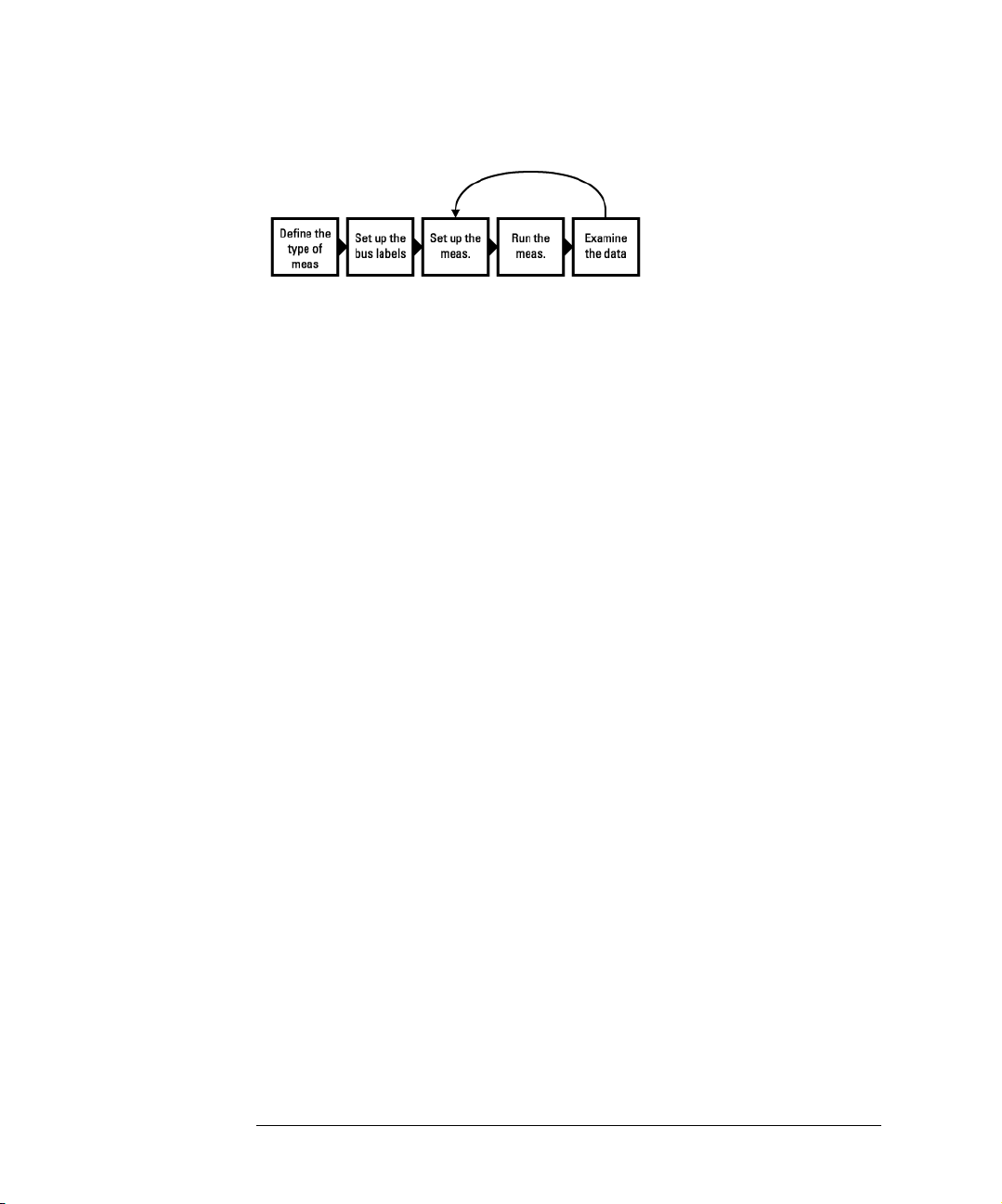
Getting Started

After you have connected the logic analyzer probes to your device under test (see “Step 1. Connect logic analyzer to the device under test” on page 15), all measurements will have the following initial steps:

Chapter 1: Getting Started

• “Step 2. Choose the sampling mode” on page 16

• “Step 3. Format labels for the probed signals” on page 19

In the timing (asynchronous) or state (synchronous) sampling modes, measurements will have these steps:

• “Step 4. Define the trigger condition” on page 22

• “Step 5. Run the measurement” on page 23

• “Step 6. Display the captured data” on page 24

In the eye scan sampling mode, measurements will have these steps:

• “Step 4. Select channels for the eye scan measurement” on page 26

• “Step 5. Set the eye scan range and resolution” on page 27

• “Step 6. Run the eye scan measurement” on page 28

• “Step 7. Display the captured eye scan data” on page 29

If you have previously saved a logic analyzer setup to a configuration file, or if configuration files are included with an analysis probe, you can load the configuration file to set up the logic analyzer and the measurement.

Once you have made a logic analyzer measurement, the measurement can be refined by repeating the measurement set up, run, and display steps.

Next: “Step 1. Connect logic analyzer to the device under test” on page 15

Chapter 1: Getting Started

Probing and Sampling Mode Selection Steps

You will always take the following steps regardless of the sampling mode you plan to use.

• “Step 1. Connect logic analyzer to the device under test” on page 15

• “Step 2. Choose the sampling mode” on page 16

• “Step 3. Format labels for the probed signals” on page 19

Step 1. Connect logic analyzer to the device under test

Before you begin setting up the logic analyzer for a measurement, you need to physically connect the logic analyzer to your device under test.

There are four probing options available to connect your logic analyzer to the device under test:

• Single-ended probes with Samtec connectors (see page 35).

• Differential probes with Samtec connectors (see page 37).

• Single-ended probes with MICTOR connectors (see page 39).

•Use an analysis probe to connect to microprocessors and standard buses. When using an analysis probe, the Setup Assistant guides you through the connection and setup process for your particular logic analyzer and analysis probe.

Next: “Step 2. Choose the sampling mode” on page 16

Chapter 1: Getting Started

Probing and Sampling Mode Selection Steps

Step 2. Choose the sampling mode

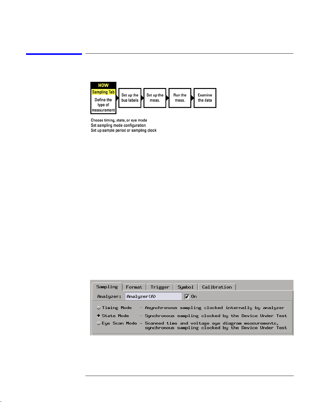
There are three logic analyzer sampling modes to choose from: timing mode, state mode, and eye scan mode.

In timing mode, the logic analyzer samples asynchronously, based on an internally-generated sampling clock.

In state mode, the logic analyzer samples synchronously, based on a sampling clock signal from the device under test. Typically, the signal used for sampling in state mode is a state machine or microprocessor clock signal.

In eye scan mode, the logic analyzer samples small windows of time and voltage on data channels around a clock signal from the device under test. The resulting eye diagrams let you validate and characterize the data valid windows of signals latched on the clock.

To choose the sampling mode

1. In the Sampling tab, choose Timing Mode, State Mode, or Eye Scan Mode.

Chapter 1: Getting Started

Probing and Sampling Mode Selection Steps

If you chose Timing Mode

1. Select the timing analyzer conventional/transitional configuration.

In the transitional timing configuration, the logic analyzer can capture a greater period of execution because only transitions are stored in memory.

2. If you chose the transitional timing configuration, set the sample period.

To capture signal level changes reliably, the sample period should be less than half (many engineers prefer one-fourth) of the period of the fastest signal you want to measure.

If you chose State Mode

1. Select the state analyzer speed configuration.

There are trade-offs between high-speed sampling, the number of available channels, triggering capabilities, and other logic analyzer characteristics. For example, in the 1250 Mb/s configuration, a periodic clock input signal is required.

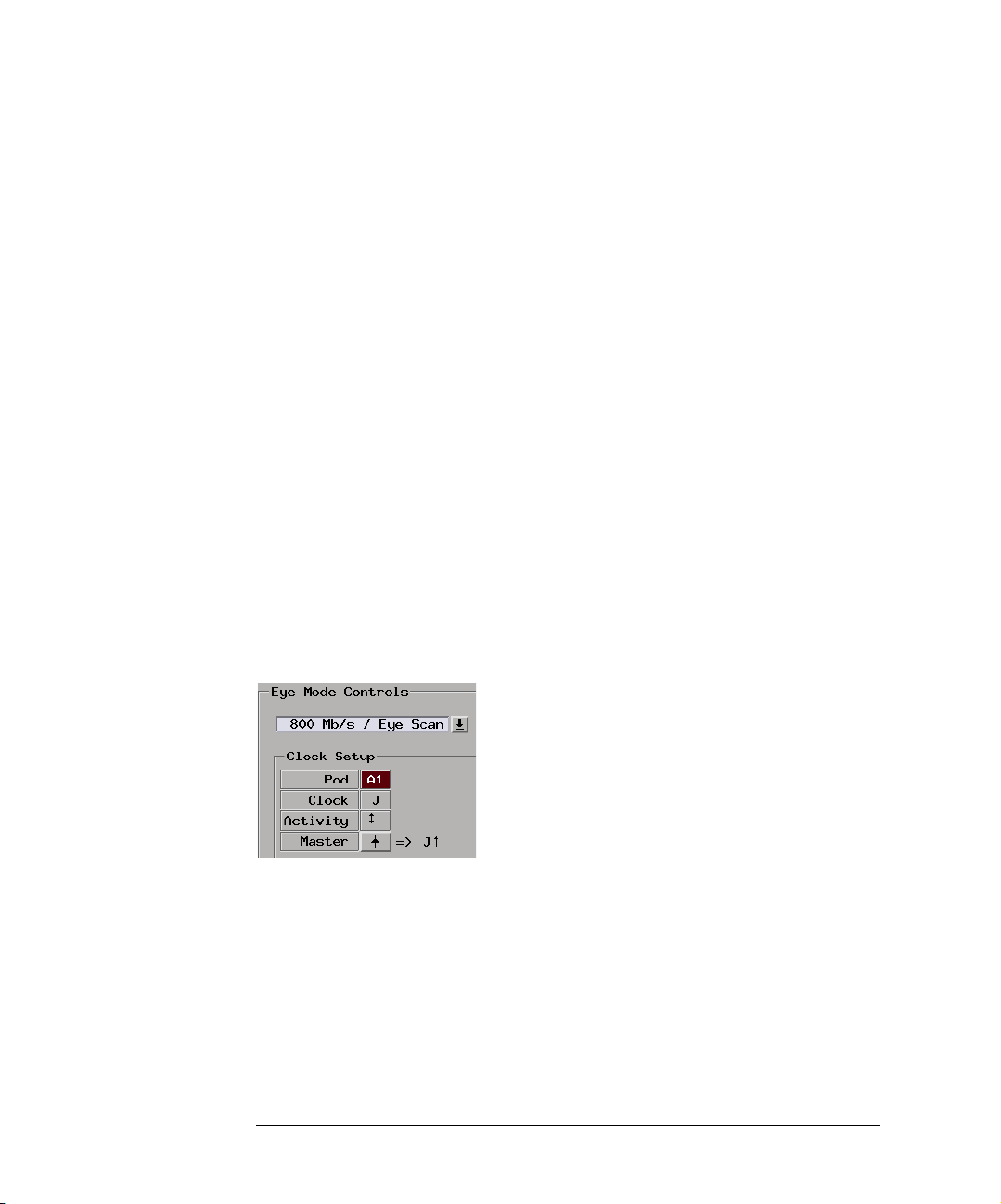
2. In the Clock Setup, specify which clock signal edges from the device under test will be used as the sampling clock.

Chapter 1: Getting Started

Probing and Sampling Mode Selection Steps

3. Specify the sampling position. Select the Sampling Positions... button, then select the Run Eye Finder button to locate the data valid window in relation to the sampling clock, and automatically set the sampling position of the logic analyzer.

See Also “To automatically adjust sampling positions” on page 49

In either Timing Mode or State Mode

1. Specify the trigger position.

The trigger is the event in the device under test that you want to capture data around.

Specify whether you want to look at data after the trigger (Start), before and after the trigger (Center), before the trigger (End), or use a percentage of the logic analyzer's memory for data after the trigger (User Defined).

2. Set the acquisition memory depth.

If you need less data and want measurements to run faster, you can limit the amount of trace memory that is filled with samples.

If you chose Eye Scan Mode

1. Select the eye scan mode speed configuration.

There are trade-offs between high-speed sampling, the number of available channels, and other logic analyzer characteristics.

2. In the Clock Setup, specify which clock signal edges from the device under test will be used as the reference clock for the eye scan measurement.

Next: “Step 3. Format labels for the probed signals” on page 19

Chapter 1: Getting Started

Probing and Sampling Mode Selection Steps

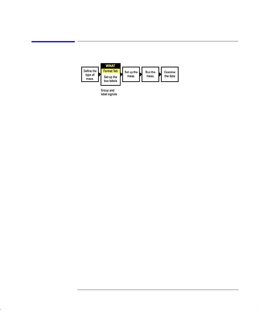
Step 3. Format labels for the probed signals

When a logic analyzer probes hundreds of signals in a device under test, you need to be able to give those channels more meaningful names than "pod 1, channel 1".

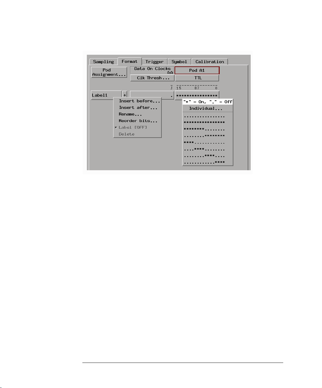
The Format tab is mainly used for assigning bus and signal names (from the device under test) to logic analyzer channels. These names are called labels. Labels are also used when setting up triggers and displaying captured data.

The Format tab also lets you do things like assign pods to the logic analyzer and specify the logic analyzer threshold voltage.

The Format tab has activity indicators that show whether the signal a channel is probing is above the threshold voltage (high), below the threshold voltage (low), or transitioning.

Chapter 1: Getting Started

Probing and Sampling Mode Selection Steps

To assign pods to the logic analyzer

1. In the Format tab, select the Pod Assignment button.

2. In the Pod Assignment dialog, drag a pod to the appropriate logic analyzer.

3. Select the Close button.

To specify threshold voltages

The threshold voltage is the voltage level that a signal must cross before the logic analyzer recognizes a change in logic levels.

1. In the Format tab, select the button under the pod name.

2. In the Pod threshold dialog, select a Standard, External Ref, Differential, or a User Defined threshold voltage.

3. Select the Close button.

4. Select the Clk Thresh button.

5. In the Clock Thresholds dialog, select the button of the clock whose threshold you wish to set.

6. In the J, K, etc., threshold dialog, select a Standard, Differential, or a User

Chapter 1: Getting Started

Probing and Sampling Mode Selection Steps

Defined threshold voltage.

7. Select the Close button.

8. Select the Close button.

To assign names to logic analyzer channels

1. Select a label button, and either:

• Choose the Rename command, enter the label name, and select the OK button.

• Or, choose the Insert before or Insert after command, enter the label name, and select the OK button.

2. In the label row, select the button of the pod that contains the channels you want to assign.

3. Either choose one of the standard channel assignments--dots (.) mean the channel is unassigned, asterisks (*) mean the channel is assigned--or choose Individual.

If you chose Individual:

a. In the "label - pod" dialog, select the channels you want to assign/

unassign.

b. Select the OK button.

• If you are using the logic analyzer in timing mode or in state mode, go to “Step 4. Define the trigger condition” on page 22.

• If you are using the logic analyzer in eye scan mode, go to “Step 4. Select channels for the eye scan measurement” on page 26.

Chapter 1: Getting Started

Timing Mode or State Mode Steps

When you have selected the timing or state sampling modes, you need to perform the following steps.

• “Step 4. Define the trigger condition” on page 22

• “Step 5. Run the measurement” on page 23

• “Step 6. Display the captured data” on page 24

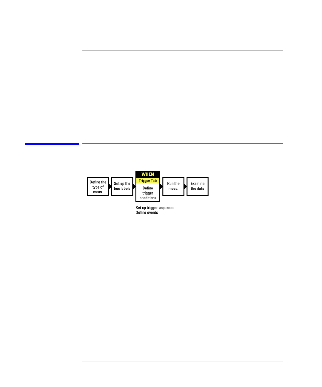
Step 4. Define the trigger condition

The trigger is the event in the device under test that you want to capture data around.

1. In the Trigger tab, and in the Trigger Functions subtab, choose the type of trigger you want to specify, and select the Replace button.

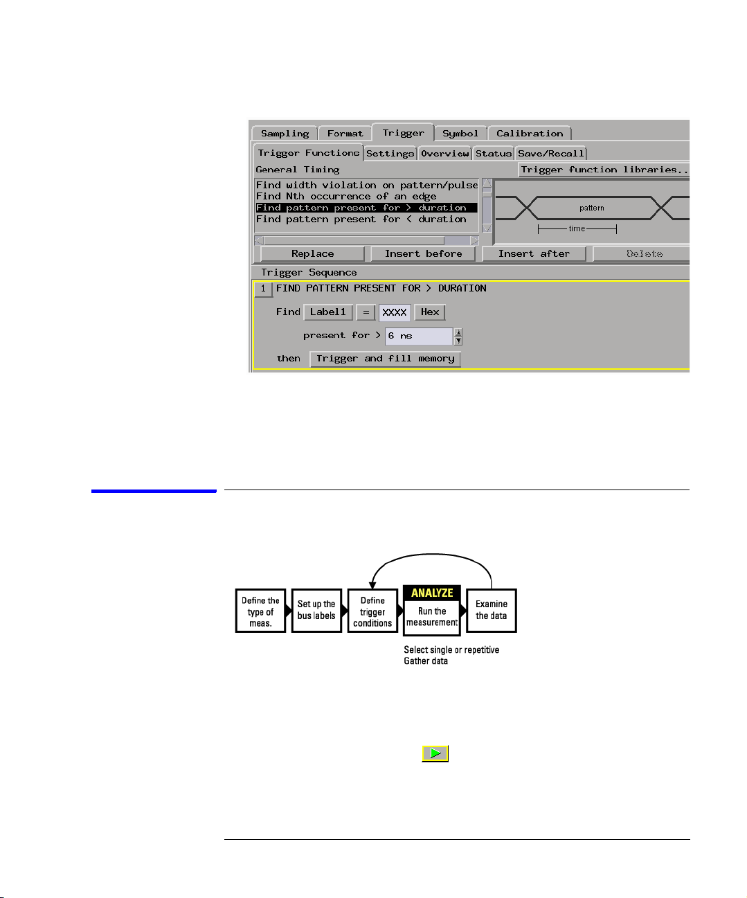
Chapter 1: Getting Started

Timing Mode or State Mode Steps

2. In the Trigger Sequence portion of the Trigger tab, select the buttons to define the label values and/or other conditions you want to trigger on.

Next: “Step 5. Run the measurement” on page 23

Step 5. Run the measurement

Once the trigger condition has been defined, you can run the measurement.

1. Select the Run Single button .

When you run a measurement, the Stop button becomes available while the logic analyzer looks for the trigger condition.

Chapter 1: Getting Started

Timing Mode or State Mode Steps

Logic analyzers with deep acquisition memory take a noticeable amount of time to complete a run; however, messages like "Waiting in level 1" may indicate you need to stop the measurement and refine the trigger condition.

When the trigger condition is found, logic analyzer acquisition memory is filled, the captured data is processed to the display tools, and the Run Single button becomes available again.

Next: “Step 6. Display the captured data” on page 24

Step 6. Display the captured data

Once you have run a measurement and filled the logic analyzer's acquisition memory with captured data, you can display it with one of the display tools.

To open Waveform or Listing displays

Waveform displays are typically used when data is captured with the timing sampling mode, and Listing displays are used when data is captured with the state sampling mode.

1. From the Window menu, select your logic analyzer and choose the Waveform or Listing command.

Chapter 1: Getting Started

Timing Mode or State Mode Steps

To add display tools via the Workspace window

1. Select the Workspace button (or from the Window menu, select System and Workspace).

2. In the Workspace window, scroll down to the Display portion of the tool icon list.

3. Drag the display tool icon and drop it on the analyzer icon.

4. To open the display tool, select its icon and choose the Display command.

Next: “For More Information...” on page 31

Chapter 1: Getting Started

Eye Scan Mode Steps

When you have selected the eye scan sampling mode, you need to perform the following steps.

• “Step 4. Select channels for the eye scan measurement” on page 26

• “Step 5. Set the eye scan range and resolution” on page 27

• “Step 6. Run the eye scan measurement” on page 28

• “Step 7. Display the captured eye scan data” on page 29

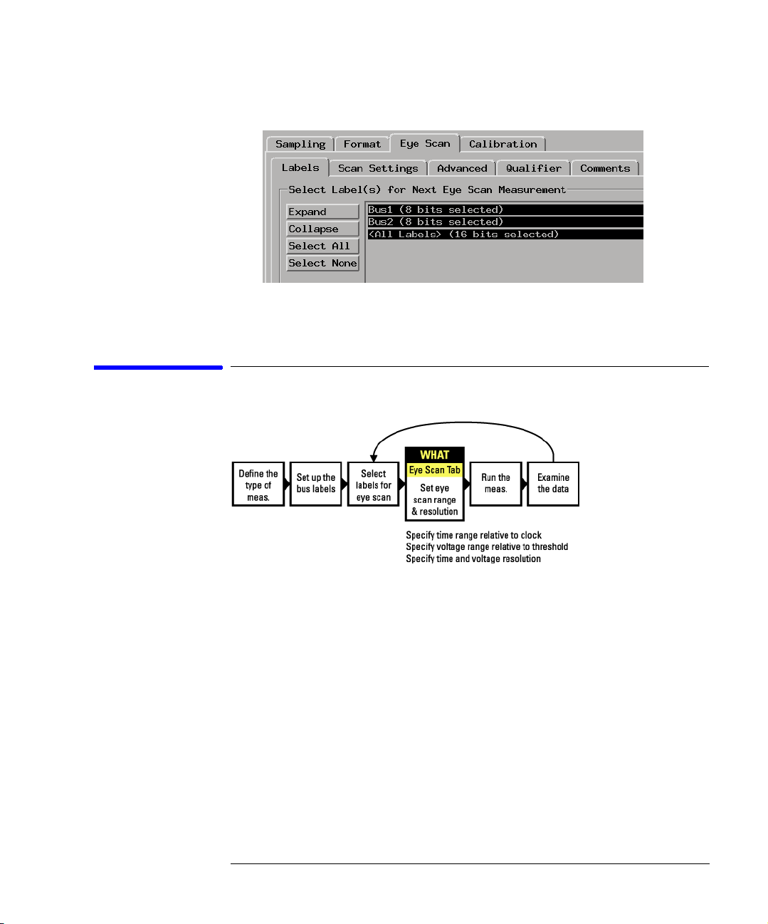
Step 4. Select channels for the eye scan measurement

1. In the Eye Scan tab, Labels subtab, select the channels you want in the eye scan measurement.

Chapter 1: Getting Started

Eye Scan Mode Steps

Next: “Step 5. Set the eye scan range and resolution” on page 27

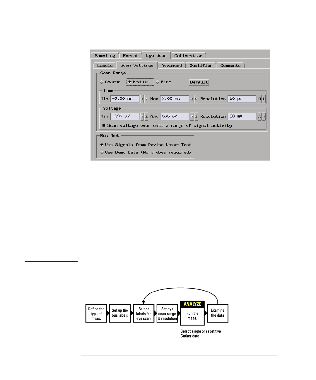
Step 5. Set the eye scan range and resolution

1. In the Eye Scan tab, Scan Settings subtab, select the settings for the eye scan measurement.

Chapter 1: Getting Started

Eye Scan Mode Steps

These settings define the number and size of the time and voltage windows used in the eye scan.

Measurements using the coarse settings run faster because there are fewer time and voltage windows to scan, but the resulting eye diagrams have less resolution.

Measurements using the fine settings result in eye diagrams with better resolution, but the measurements take longer to run because there are more time and voltage windows to scan.

Next: “Step 6. Run the eye scan measurement” on page 28

Step 6. Run the eye scan measurement

Chapter 1: Getting Started

Eye Scan Mode Steps

Once the eye scan settings have been selected, you can run the measurement.

1. Select the Run Single button .

The Eye Scan display window opens, and the captured measurement data begins to appear.

While the eye scan measurement runs, the Stop button becomes available.

The estimated time of the measurement is shown in the status field.

Next: “Step 7. Display the captured eye scan data” on page 29

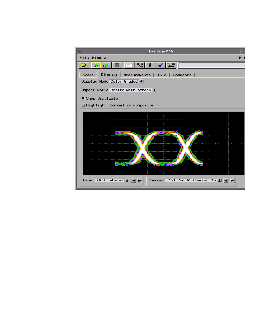
Step 7. Display the captured eye scan data

Chapter 1: Getting Started

Eye Scan Mode Steps

In the Eye Scan display window, use the following subtabs:

• Scale to zoom in or out on the captured data.

• Display to change the display options.

• Measurements to use tools for displaying useful information about the data.

• Info to display textual information about the captured measurement data.

• Comments to save your comments with the data.

Next: “For More Information...” on page 31

For More Information...

Chapter 1: Getting Started

For More Information...

On connecting the logic analyzer:

On choosing the sampling mode:

On formatting labels for probed signals:

On setting up measurements:

• “Probing the Device Under Test” on page 35

• Setup Assistant (see the Setup Assistant help volume) (when using analysis probes).

• Logic Analysis System and Measurement Modules Installation Guide for probe pinout and circuit diagrams.

• “Choosing the Sampling Mode” on page 43

• “The Sampling Tab” on page 155

• “Formatting Labels for Logic Analyzer Probes” on page 57

• “The Format Tab” on page 174

• “Understanding Logic Analyzer Triggering” on page 240

• “Understanding Eye Scan Measurements” on page 259

• “Setting Up Triggers and Running Measurements” on page 69

• “Setting Up and Running Eye Scan Measurements” on page 119

• “The Trigger Tab” on page 176

• “The Eye Scan Tab” on page 204

On running measurements:

On displaying captured data:

• “Running Measurements” on page 91

• “To run an eye scan measurement” on page 121

• “Displaying Captured Data” on page 94

• “Displaying Captured Eye Scan Data” on page 133

• Using the Waveform Display Tool (see the Waveform Display Tool help volume)

• Using the Listing Display Tool (see the Listing Display Tool help volume)

• Working with Markers (see the Markers help volume)

Chapter 1: Getting Started

For More Information...

• Using the Chart Display Tool (see the Chart Display Tool help volume)

• Using the Distribution Display Tool (see the Distribution Display Tool help volume)

• Using the Compare Analysis Tool (see the Compare Tool help volume)

Probing and Selecting the Sampling Mode

• “Probing the Device Under Test” on page 35

Chapter 2: Probing and Selecting the Sampling Mode

• “Choosing the Sampling Mode” on page 43

• “Selecting the Timing Mode (Asynchronous Sampling)” on page 43

• “Selecting the State Mode (Synchronous Sampling)” on page 46

• “In Either Timing Mode or State Mode” on page 53

• “Selecting the Eye Scan Mode” on page 55

• “Formatting Labels for Logic Analyzer Probes” on page 57

Chapter 2: Probing and Selecting the Sampling Mode

Probing the Device Under Test

When using the 16760A logic analyzer, there are four probing options available:

• “Using the E5378A Single-Ended Probe” on page 35

• “Using the E5379A Differential Probe” on page 37

• “Using the E5380A Mictor-Compatible Probe” on page 39

• “Using the E5382A Single-ended Flying Lead Probe Set” on page 40

• “Using an Analysis Probe” on page 41

Using the E5378A Single-Ended Probe

Mechanical Considerations

The E5378A single-ended probe has 34-channels and is capable of capturing data at rates up to 1500 Mb/s. The probe has the following inputs:

• 32 single-ended data inputs, in two groups (pods) of 16.

• Two differential clock inputs. Either or both clock inputs can be acquired as data inputs if not used as a clock.

• Two data threshold reference inputs, one for each pod (group of 16 data inputs).

This probe matches two 17-channel probe cables to a single-ended 100-pin Samtec connector.

Each E5379A probe requires a mating connector and support shroud built into the device under test.

You can order a probing connector kit, which contains five mating connectors and five support shrouds, using the Agilent part numbers:

• 16760-68702 for PC board thicknesses up to 0.062 in.

• 16760-68703 for PC board thicknesses up to 0.120 in.

Chapter 2: Probing and Selecting the Sampling Mode

Probing the Device Under Test

You can order mating connectors separately using the Agilent part number:

• 1253-3620 (or Samtec #ASP-65067-01)

You can order support shrouds separately using the Agilent part numbers:

• 16760-02302 for PC board thicknesses up to 0.062 in.

• 16760-02303 for PC board thicknesses up to 0.120 in.

Electrical Considerations

Data threshold reference inputs

The E5378A single-ended probe has two inputs for threshold reference voltages for the data inputs. One input is for the even pod and the other is for the odd pod. The threshold inputs (pins 87 and 88) may be either:

Connected to a DC threshold reference voltage. In this case, the logic analyzer will use the threshold reference voltage to determine when the signal is high or low.

Or:

Grounded or left unconnected. In this case, you need to set the logic threshold voltage in the user interface.

The advantages of supplying a threshold voltage via the threshold input on the probe are:

• A threshold voltage supplied from the device under test will typically track changes in supply voltage, temperature, etc.

• A threshold voltage supplied from the device under test is typically the same threshold that the device's logic uses to evaluate the signals. Therefore, the data captured by the logic analyzer will be the same as the data interpreted by the device under test.

Clock Input

The clock input on the E5378A probe can be a differential signal or a single-ended signal.

If the clock input is a differential signal, select the "differential" option in the clock threshold user interface.

Chapter 2: Probing and Selecting the Sampling Mode

If the clock input is a single-ended signal, either ground the negative clock input and adjust the clock threshold voltage in the user interface, or connect the negative clock input to the DC clock threshold reference voltage.

In the user interface, the clock input threshold voltage adjustment is separate from the data input threshold voltage adjustments.

See Also “To set pod threshold voltages” on page 58

“To set clock threshold voltages” on page 59

For complete information, including mechanical considerations such as pin-out and footprint and electrical considerations such as circuit board design best practices, refer to the Agilent Technologies E5378A, E5379A, and E5380A Probes for the 16760A Logic Analyzer user's guide that comes with the probes.

Probing the Device Under Test

Mechanical Considerations

Using the E5379A Differential Probe

The E5379A differential probe has 17 channels and is capable of capturing data at rates up to 1500 Mb/s. The probe has the following inputs:

• 16 differential data inputs.

• One differential clock input. The clock input can also be used as a data input.

This probe matches one 17-channel probe cable to a differential 100pin Samtec connector. Two E5379A probes are required to support the inputs on one 16760A logic analyzer card.

Each E5379A probe requires a mating connector and support shroud built into the device under test.

You can order a probing connector kit, which contains five mating connectors and five support shrouds, using the Agilent part numbers:

• 16760-68702 for PC board thicknesses up to 0.062 in.

• 16760-68703 for PC board thicknesses up to 0.120 in.

Chapter 2: Probing and Selecting the Sampling Mode

Probing the Device Under Test

You can order mating connectors separately using the Agilent part number:

• 1253-3620 (or Samtec #ASP-65067-01)

You can order support shrouds separately using the Agilent part numbers:

• 16760-02302 for PC board thicknesses up to 0.062 in.

• 16760-02303 for PC board thicknesses up to 0.120 in.

Electrical Considerations

Data inputs

The E5379A differential probe can capture data on differential signals or single-ended signals.

When capturing data on differential signals, the logic analyzer will determine high and low states based on the crossover of the data and negative data inputs.

When capturing data on single-ended signals, either ground the negative data inputs and adjust the threshold voltage in the user interface, or connect the negative data inputs to the DC threshold reference voltage.

Clock input

The clock input on the E5379A differential probe can also be a differential signal or a single-ended signal, in the same way as described for the data inputs above. The clock input has a separate, independent threshold adjustment.

See Also “To set pod threshold voltages” on page 58

“To set clock threshold voltages” on page 59

Chapter 2: Probing and Selecting the Sampling Mode

Probing the Device Under Test

Using the E5380A Mictor-Compatible Probe

The E5380A MICTOR-compatible probe has a MICTOR connector end. If you have a device under test with connectors designed for the Agilent E5346A high-density probe adapter, you can also use the E5380A probe.

However, the lower bandwidth of the E5380A probe limits the maximum state speed of the logic analyzer to 600 Mbits/second.

The minimum input signal amplitude required by the E5380A probe is 300 mV.

The probe matches two 17-channel probe cables to a single-ended 38 pin MICTOR connector.

Mechanical Considerations

Electrical Considerations

Each E5380A probe requires a MICTOR connector and support shroud built into the device under test.

You can order a probing connector kit, which contains five MICTOR connectors and five support shrouds, using the Agilent part numbers:

• E5346-68701 for PC board thicknesses up to 0.062 in.

• E5346-68702 for PC board thicknesses from 0.062 to 0.125 in.

You can order MICTOR connectors separately using the Agilent part number:

• 1252-7431 (or AMP part #2-767004-2)

You can order support shrouds separately using the Agilent part numbers:

• E5346-44701 for PC board thicknesses up to 0.062 in.

• E5346-44704 for PC board thicknesses from 0.062 to 0.125 in.

• E5346-44703 for PC board thicknesses from 0.125 to 0.70 in.

All inputs on the E5380A MICTOR-compatible probe are single-ended. The E5380A probe does not have a threshold reference voltage input. When using the E5380A probe, the logic threshold voltage is adjusted in the user interface.

Chapter 2: Probing and Selecting the Sampling Mode

Probing the Device Under Test

The clock input on the E5380A probe is single-ended. The clock threshold voltage may be adjusted independently of the data threshold voltages.

See Also “To set pod threshold voltages” on page 58

“To set clock threshold voltages” on page 59

Using the E5382A Single-ended Flying Lead Probe Set

Mechanical Considerations

Electrical Considerations

Clock Input

The E5382A is a 17-channel single-ended flying lead probe set. The E5382A lets you acquire signals from randomly located points in your target system. Two E5382As are required to support 34 channel logic analyzer cards. Four are required to support 68-channel logic analyzer cards.

The Agilent E5382A single-ended flying lead probe set comes with accessories that trade off flexibility, ease of use, and performance. Discussion and comparisons between four of the most common intended uses of the accessories are included in the E5382A Single- ended Flying Lead Probe Set User's Guide (supplied with the probe). A list of replacable parts and additional accessories is given below.

Data inputs on the E5382A flying lead probe are single-ended. The E5382A probe does not have a threshold reference voltage input. When using the E5382A probe, the logic threshold voltage is adjusted in the user interface.

The maximum nondestructive input voltage is +/- 40 Vdc.

The clock input on the E5382A probe can be a differential signal or a

Chapter 2: Probing and Selecting the Sampling Mode

Probing the Device Under Test

single-ended signal. If the clock input is a differential signal, select the "differential" option in the clock threshold user interface.

If the clock input is a single-ended signal, ground the negative clock input and adjust the clock threshold voltage in the user interface. The minimum voltage swing for single-ended clock operation is 250 mV p-p.

In the user interface, the clock input threshold voltage adjustment is separate from the data input threshold voltage adjustments.

Replacable Parts and Additional Accessories

A variety of accessories are supplied with the E5382A to allow you to access signals on various types of components on your PC board. The following table shows the part numbers for ordering replacement parts and additional accessories.

Description Qty Agilent Part Number

-------------- --- -------------------

Probe Pin Kit 4 16517-82107

High Frequency Probing Kit 8 16517-82104 (4 resistive signal pins & 4 solder-down grounds)

Ground Extender 20 16517-82105

Grabber Clip Kit 20 16517-92109

Right-angle Ground Lead 20 16517-82106

Cable - Main 1 E5382-61601

Probe Tip to BNC Adapter 1 E9638A

Using an Analysis Probe

Analysis probes, formerly called preprocessors, are products that make it easier to probe a specific microprocessor or bus.

Generally, analysis probes consist of hardware that probes a microprocessor or bus and routes the probed signals to connectors for the logic analyzer probe cables.

Analysis probes include configuration files that properly set up the logic analyzer. Also included, typically, are inverse assemblers or other tools for decoding the captured data.

The Setup Assistant (see the Setup Assistant help volume) in the logic

Chapter 2: Probing and Selecting the Sampling Mode

Probing the Device Under Test

analysis system helps you to properly configure the logic analyzer.

Chapter 2: Probing and Selecting the Sampling Mode

Choosing the Sampling Mode

There are three logic analyzer sampling modes to choose from: timing mode, state mode, or eye scan mode.

In timing mode, the logic analyzer samples asynchronously, based on an internally-generated sampling clock.

In state mode, the logic analyzer samples synchronously, based on a sampling clock signal (or signals) from the device under test. Typically, the signal used for sampling in state mode is a state machine or microprocessor clock signal.

• “Selecting the Timing Mode (Asynchronous Sampling)” on page 43

• “Selecting the State Mode (Synchronous Sampling)” on page 46

• “In Either Timing Mode or State Mode” on page 53

• “Selecting the Eye Scan Mode” on page 55

Selecting the Timing Mode (Asynchronous Sampling)

In timing mode, the logic analyzer samples asynchronously, based on an internally-generated sampling clock.

• “To select the timing mode” on page 44

• “To select the conventional/transitional configuration” on page 44

• “To specify the sample period” on page 45

Chapter 2: Probing and Selecting the Sampling Mode

Choosing the Sampling Mode

To select the timing mode

1. Open the logic analyzer Setup window.

2. Select the Sampling tab.

3. Choose the Timing Mode option.

You can also select the timing sampling mode in the “Pod Assignment Dialog” on page 175.

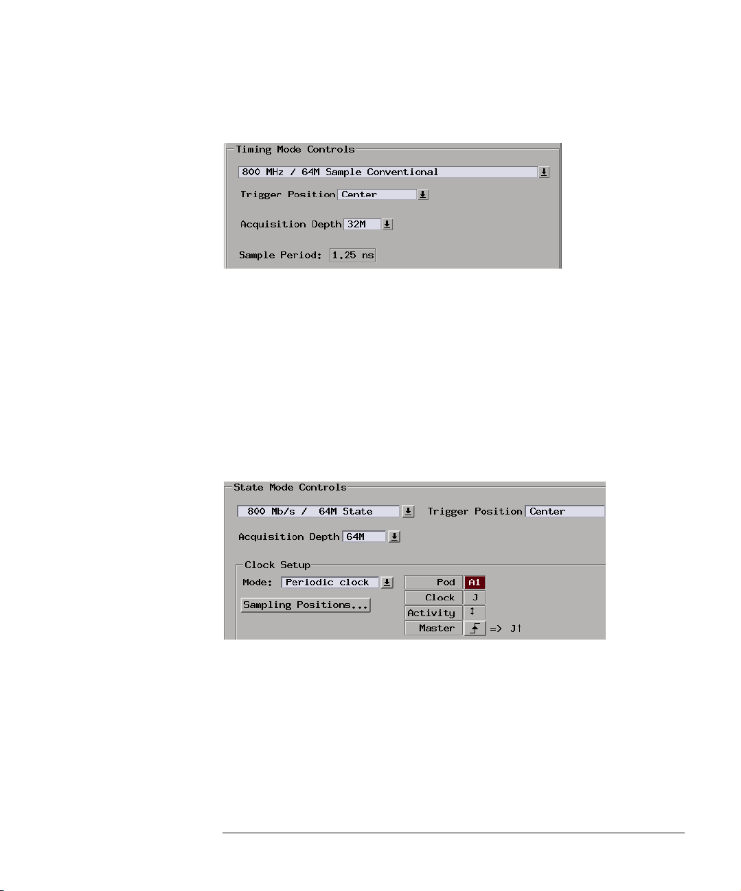
To select the conventional/transitional configuration

1. In the Sampling tab with Timing Mode selected, select the timing analyzer configuration. You can choose between:

• 800 MHz / 64M Sample Conventional

In this configuration, the analyzer samples and stores measurement data at each sampling interval, as often as every 1.25 ns.

NOTE: With the Sample Period at 1.25 ns, data is acquired at four times the trigger

sequencer rate. This means that data must be present for at least four samples before the trigger sequencer can reliably detect it. The trigger sequencer could miss data present for less than four sample periods.

The trigger sequencer treats the data as a group of four samples for each sequencer clock. This means that the trigger point indication could be off by three samples.

Although the trigger sequencer cannot detect all data, the analyzer will correctly capture all data present for at least one sample period.

• 400 MHz / 32M Sample Transitional or Store Qualified

In this configuration, the analyzer samples data at regular intervals, as often as every 2.5 ns, but only stores the data if it's different than the previously stored data.

You can further qualify storage of transitions by ignoring data changes on particular labels.

A time tag is stored with each stored data sample so that all sampled values can be reconstructed and displayed later.

Chapter 2: Probing and Selecting the Sampling Mode

Choosing the Sampling Mode

NOTE: If all pods are used, memory depth is reduced by half in order to store the

required time tags.

NOTE: With the Sample Period at 2.5 ns, data is acquired at two times the trigger

sequencer rate. This means that data must be present for at least two samples before the trigger sequencer can reliably detect it. The trigger sequencer could miss data present for less than two sample periods.

The trigger sequencer treats the data as a group of two samples for each sequencer clock. This means that the trigger point indication could be off by one sample.

Although the trigger sequencer cannot detect all data, the analyzer will correctly capture all data present for at least one sample period.

See Also “To specify default storing” on page 76

“How Samples are Stored in Transitional Timing” on page 157

“Default Storing Subtab” on page 190

To specify the sample period

When the logic analyzer is in timing (asynchronous sampling) mode, the Sample Period setting specifies how often the logic analyzer samples the signals from the device under test.

1. In the Sampling tab, with Timing Mode selected, enter the desired time between logic analyzer samples.

To capture signal level changes reliably, the sample period should be less than half (many engineers prefer one-fourth) of the period of the fastest signal you want to measure.

The sample rate is the inverse of the sample period.

NOTE: In the conventional timing configuration, the sample rate is fixed at 1.25 ns.

Chapter 2: Probing and Selecting the Sampling Mode

Choosing the Sampling Mode

Selecting the State Mode (Synchronous Sampling)

The clock signal can be either Periodic (synchronous all the time), or Aperiodic (bursted or varying in frequency).

• “To select the state mode” on page 47

• “To select the state speed configuration” on page 47

• “To set up the sampling clock” on page 48

State Mode Sampling Position

In order for a state mode logic analyzer to accurately capture data from a device under test, the logic analyzer's setup/hold time (window) must fit within the device under test's data valid window.

Because the location of the data valid window relative to the bus clock is different for different types of buses, the logic analyzer lets you adjust the sampling position in order to accurately capture data on high-speed buses (see “Understanding State Mode Sampling Positions” on page 256).

When the device under test's data valid window is less than 2.5 ns (roughly, for clock speeds >= 200 MHz), it's easiest to use eye finder to locate the stable and transitioning regions of signals and to automatically adjust sampling positions.

• “To automatically adjust sampling positions” on page 49

When the device under test's data valid window is greater than 2.5 ns (roughly, for clock speeds < 200 MHz), it's easiest to adjust the sampling position manually, without using the logic analyzer to locate the stable and transitioning regions of signals.

• “To manually adjust sampling positions” on page 52

Chapter 2: Probing and Selecting the Sampling Mode

Choosing the Sampling Mode

To select the state mode

1. Open the logic analyzer Setup window.

2. Select the Sampling tab.

3. Choose the State Mode option.

You can also select the state sampling mode in the “Pod Assignment Dialog” on page 175.

To select the state speed configuration

1. In the Sampling tab, with State Mode selected, select one of the state analyzer configurations.

The selected configuration specifies the speed up to which the state mode sampling clock will match input clock edges from the device under test. For example, in the 800 Mb/s / 64M State configuration, the state mode sampling clock will match input clock edges up to 800 MHz.

The selected configuration also specifies the memory depth for samples and whether only half of the logic analyzer channels are available.

You can choose from:

• 1500 Mb/s / 128M Half Channel

In this configuration: The input clock signal must be periodic, and both edges indicate valid data. The clock input can only be used as a clock and not as an extra data channel. The logic analyzer setup/hold window is 500 ps, and eye finder must be used to automatically adjust sampling positions. The limited set of 16760 Half Channel State trigger functions are available. In half-channel mode the analyzer accesses only the even channels (0, 2, 4, etc.).

• 1250 Mb/s / 128M Half Channel

In this configuration: The input clock signal must be periodic, and both edges indicate valid data. The clock input can only be used as a clock and not as an extra data channel. The logic analyzer setup/hold window is 1 ns, and sampling positions may be adjusted automatically or manually. The limited set of 16760 Half Channel State trigger functions are available. In half-channel mode the analyzer accesses only the even channels (0, 2, 4, etc.).

Chapter 2: Probing and Selecting the Sampling Mode

Choosing the Sampling Mode

• 800 Mb/s / 64M State

In this configuration: The input clock signal can be periodic or aperiodic, and either rising, falling, or both edges can indicate valid data. The logic analyzer setup/hold window is 1 ns, and sampling positions may be adjusted automatically or manually. The limited set of 16760 State trigger functions are available.

• 400 Mb/s / 32M State

In this configuration: Either rising, falling, or both edges can indicate valid data. The logic analyzer setup/hold window is 2.5 ns, and sampling positions may be adjusted automatically or manually. The limited set of Turbo State trigger functions are available.

• 200 Mb/s / 32M State

In this configuration: Rising, falling, or both edges can indicate valid data. The logic analyzer setup/hold window is 3.0 ns, and sampling positions may be adjusted automatically or manually. The General State trigger functions are available.

In all configurations but the 200 Mb/s / 32M State configuration, if time is counted (that is time tags are being stored), one pod must be left unassigned in order to store the time tags. In the 200 Mb/s / 32M State configuration, memory depth is reduced by half if all pods are used and time or state counts are being stored.

See Also “To set up the sampling clock” on page 48

“To manually adjust sampling positions” on page 52

“To automatically adjust sampling positions” on page 49

“Trigger Functions Subtab” on page 177

To set up the sampling clock

For the clock input signal that will be used:

1. In the Clock Setup, select the desired Mode. Your choices are Periodic or Aperiodic. If the State Mode is set to 1250 or 1500 Mb/s configuration, the input clock must be Periodic.

2. Select the pod's Master button (under the activity indicator).

Chapter 2: Probing and Selecting the Sampling Mode

Choosing the Sampling Mode

3. Specify when to sample. Your choices are Rising Edge, Falling Edge, or Both Edges. Only Both Edges is available in the 1250 and 1500 Mb/s

configurations.

See Also “To select the state speed configuration” on page 47

To automatically adjust sampling positions

When adjusting the state mode sampling position with eye finder, the logic analyzer looks at signals from the device under test, figures out the location of the data valid window in relation to the sampling clock, and automatically sets the sampling position.

Because eye finder automatically runs on individual channels, it can correct for the small delay effects caused by probe cables and circuit board traces. This makes the logic analyzer's setup/hold window smaller and lets you accurately capture data at higher clock speeds.

Eye finder requires:

• At least 500 transitions on each signal during its run. (You can use the advanced eye finder settings to cause longer or shorter runs.)

• All devices which can drive each signal should contribute to the stimulus.

• All device under test operating modes relevant to the eventual logic analysis measurement should contribute to the stimulus as well.

NOTE: Eye finder measurements and normal logic analyzer measurements cannot

run simultaneously.

To run eye finder

1. Probe the device under test by connecting the logic analyzer channels.

2. Select the state (synchronous sampling) mode (see “To select the state mode” on page 47).

3. Format labels for those logic analyzer channels.

4. Make sure that the device under test and the logic analyzer have warmed up to their normal operating temperatures.

5. In the Format tab, select the Setup/Hold button.

Chapter 2: Probing and Selecting the Sampling Mode

Choosing the Sampling Mode

6. In the Sampling Positions dialog, select the Eye Finder option.

7. In the Eye Finder Setup tab, select the Use signals from Device Under Test option.

The Use demo data (no probes required) option is for demonstration purposes only.

8. Choose the labels that you wish to run eye finder on.

You may want to run eye finder on channel subsets, for example, when certain bus signals transition in one operating mode (of the device under test) and other bus signals transition in a different operating mode.

9. Select the Run Eye Finder button.

For more information on run messages, see “Eye Finder Run Messages” on page 162.

When eye finder finds more than one stable region on a channel, it uses the current sampling position as a hint about which stable region it should suggest a position for.

If eye finder picks the wrong stable region, you can expand the label and drag the blue Sampling Position line into the correct stable region. The suggested sampling position for that region will be shown (see “How Selected/Suggested Positions Behave” on page 161).

10. If you have moved the sampling position and wish to return to the suggested positions, go to the Eye Finder Results tab, select a label button or the Results menu, and choose the "set to suggested" command.

For more information on informational messages in the Eye Finder Results tab, see “Eye Finder Info Messages” on page 165.

Eye finder finds optimal sampling positions for the actual specific conditions -- amplitude, offset, slew rates, and ambient temperature. Therefore, you will get the best results by running eye finder under the same conditions that will be present when logic analysis measurements are made.

To run eye finder repetitively

1. Select the Repetitive Run option in the Eye Finder Setup tab.

2. Select the Run Eye Finder (r) button.

Chapter 2: Probing and Selecting the Sampling Mode

Choosing the Sampling Mode

In the Eye Finder Results tab, you can see how the stable and transitioning areas vary over time.

3. Select the Stop Eye Finder button.

To view eye finder data as a bus composite

When you want a compressed, high-level view of the eye finder data:

1. In the Eye Finder Results tab, select the label button and choose the View as Bus Composite command.

Average sampling positions as well as stable and transitioning areas are displayed for the whole label. This is the default. Stable areas show positions where every channel in the label is stable.

To view eye finder data as a stack of channels

When you want more resolution in your view of the eye finder data:

1. In the Eye Finder Results tab, select the label button and choose the View as Stack of Channels command.

Individual sampling positions and stable and transitioning areas for all the channels in a label are shown.

To save/load eye finder data

While the eye finder sampling positions are saved with the logic analyzer configuration, eye finder measurement data is not; therefore,

Chapter 2: Probing and Selecting the Sampling Mode

Choosing the Sampling Mode

eye finder data must be saved and loaded separately.

1. In the File Info tab, select the Save As... or Load... buttons.

You can also choose the Save Eye Finder or Load Eye Finder command from the File menu.

2. In the file browser dialog, name the file to be saved or select the file to be loaded.

For more information on save/load messages, see “Eye Finder Load/Save Messages” on page 167.

See Also “Understanding State Mode Sampling Positions” on page 256

“Eye Finder Advanced Settings Dialog” on page 170

“To manually adjust sampling positions” on page 52

To manually adjust sampling positions

Although the Eye Finder option was intended for automatically adjusting state mode sampling positions, you can also use it to manually adjust sampling positions. You don't have to Run Eye Finder to locate stable and transitioning regions on signals, just go directly to the Eye Finder Results tab, and drag the sampling positions to the proper locations.

1. Select the state (synchronous sampling) mode (see “To select the state mode” on page 47).

2. In the Format tab, select the Setup/Hold button.

3. In the Sampling Positions dialog, select the Eye Finder option.

4. In the Eye Finder Results tab, drag the sampling positions to the proper locations.

You can select bus labels to expand or collapse the channels in the label.

When using the Eye Finder option to manually adjust state mode sampling positions, the sampling positions are saved with the logic analyzer configuration (see “Saving and Loading Logic Analyzer Configurations” on page 116).

Chapter 2: Probing and Selecting the Sampling Mode

Choosing the Sampling Mode

See Also “Understanding State Mode Sampling Positions” on page 256

“To automatically adjust sampling positions” on page 49

In Either Timing Mode or State Mode

• “To specify the trigger position” on page 53

• “To set acquisition memory depth” on page 53

• “To name an analyzer” on page 54

• “To turn an analyzer off or on” on page 54

To specify the trigger position

1. In the Sampling tab (or in the Settings subtab of the Trigger tab), select the trigger position.

In the timing sampling mode's 800 MHz / 64M Sample Conventional configuration, when a Run is started, the analyzer will not look for a trigger until the specified percentage of pretrigger data has been stored. After a trigger has been detected, the specified percentage of posttrigger data is stored before the analyzer halts. This ensures that both pretrigger and posttrigger storage are complete.

In the state sampling mode, or in the timing sampling mode's 400 MHz / 32M Sample Transitional or Store Qualified configuration, when a Run is started, the analyzer immediately looks for the trigger condition. In other words, the trigger position setting specifies the maximum amount of data that should be stored before the trigger.

To set acquisition memory depth

If you need less data and want measurements to run faster, you can limit the number of samples that are stored in logic analyzer acquisition memory.

Chapter 2: Probing and Selecting the Sampling Mode

Choosing the Sampling Mode

1. In the Sampling tab (or in the Settings subtab of the Trigger tab), select the acquisition depth.

The number of samples that can be chosen for the Acquisition Depth are approximations. The combination of count tags, pod assignments, and configuration modes affect what choices are available.

To name an analyzer

You can give more descriptive names to a logic analyzer.

1. In the Sampling tab, select the Analyzer Name field.

2. Enter the new name.

The name now appears below the instrument tool icon in the workspace.

You can also name analyzers in the “Pod Assignment Dialog” on page 175.

To turn an analyzer off or on

You may want to turn an analyzer off if you don't want it to be included in further measurements.

To turn an analyzer off

1. In the Sampling tab, select the On box that is checked.

2. In the Analyzer Shutdown Options dialog, choose either:

• Soft -- This will leave the logic analyzer window but turn off most

options.

• Hard -- This will remove the logic analyzer and its display tools from

the Workspace.

You can also turn an analyzer off in the “Pod Assignment Dialog” on page 175.

To turn an analyzer back on

1. If you used the Soft option when turning the logic analyzer off, you can turn it on again by selecting the Off check box.

2. If you used the Hard option when turning the logic analyzer off, you can

Chapter 2: Probing and Selecting the Sampling Mode

Choosing the Sampling Mode

turn it on again by selecting the Setup button in the System window or by dragging the analyzer's instrument tool icon to the workspace in the Workspace window.

Selecting the Eye Scan Mode

In eye scan mode, the logic analyzer becomes a tool for validating and characterizing the data valid windows of signals latched by a clock. The Eye Scan display shows eye diagrams for each channel, like an oscilloscope, but with less accuracy and resolution. The Eye Scan display can help you quickly identify setup/hold or other signal integrity anomalies which can then be examined in greater detail with a high-speed or high-bandwidth oscilloscope.

• “To select the eye scan mode” on page 55

• “To select the eye scan mode speed configuration” on page 55

• “To set up the eye scan mode reference clock” on page 56

See Also “Setting Up and Running Eye Scan Measurements” on page 119

“Displaying Captured Eye Scan Data” on page 133

“Saving and Loading Captured Eye Scan Data” on page 152

“Understanding Eye Scan Measurements” on page 259

To select the eye scan mode

1. Open the logic analyzer Setup window.

2. Select the Sampling tab.

3. Choose the Eye Scan Mode option.

To select the eye scan mode speed configuration

1. In the Sampling tab, with Eye Scan Mode selected, select one of the eye scan mode speed configurations.

The selected configuration specifies the speed that the input reference clock may be as fast as. For example, in the 800 Mb/s / Eye Scan

Chapter 2: Probing and Selecting the Sampling Mode

Choosing the Sampling Mode

configuration, the input reference clock edges can occur at rates up to 800 MHz.

You can choose from:

• 800 Mb/s / Eye Scan

In this configuration: Either rising, falling, or both edges of the input reference clock can indicate valid data. All of the logic analyzer channels are available. The maximum number of clocks that can be processed at each scan point is 60,000,000.

• 1500 Mb/s / Eye Scan

In this configuration: Both edges of the input reference clock indicate valid data. Only half of the logic analyzer channels are available. The maximum number of clocks that can be processed at each scan point is 120,000,000.

To set up the eye scan mode reference clock

For the clock input signal that will be used:

1. Select the pod's Master button (under the activity indicator).

2. Select whether data is valid on the Rising Edge, Falling Edge, or Both Edges.

In the 1500 Mb/s / Eye Scan speed configuration, data must be valid on Both Edges.

See Also “To select the eye scan mode speed configuration” on page 55

Chapter 2: Probing and Selecting the Sampling Mode

Formatting Labels for Logic Analyzer Probes

The Format tab is mainly for assigning bus and signal names (from the device under test), to logic analyzer channels. These names are called labels. Labels are used when setting up triggers and displaying captured data.

The Format tab also lets you do things like assign pods to the logic analyzer, specify the logic analyzer threshold voltage, change the label polarity, reorder bits in a label, and turn labels off or on.

The Format tab has activity indicators that show signal levels.

• “To assign pods to the analyzer” on page 57

• “To set pod threshold voltages” on page 58

• “To set clock threshold voltages” on page 59

• “To assign probe channels to labels” on page 60

• “To import label names and assignments from a netlist” on page 62

• “To import label definitions from an ASCII file” on page 63

• “To export label definitions to an ASCII file” on page 64

• “To change the label polarity” on page 64

• “To reorder bits in a label” on page 65

• “To turn labels off or on” on page 66

To assign pods to the analyzer

The logic analyzer pods can be assigned to the logic analyzer, or, they can be left unassigned.

1. In the Format tab, select the Pod Assignment button.

2. In the Pod Assignment dialog, drag a pod to the logic analyzer.

3. Select the Close button.

Chapter 2: Probing and Selecting the Sampling Mode

Formatting Labels for Logic Analyzer Probes

Capturing Data on 17 Channels in State Mode

On a single-card 16760A logic analyzer in the state (synchronous) sampling mode, you can assign pod 2 to the logic analyzer and unassign pod 1. (One pod must be unassigned in order to store time tags.) Even though pod 1 is unassigned, its J clock input is still used as the sampling clock input. This allows the 16 channels and the K clock input on pod 2 to be used as data sampling channels. This lets you capture data on high-speed buses that have 17 data bits, and a clock.

When you assign pods this way, the logic analyzer loses its ability to detect, to prevent triggering or sequencing on, and to remove an initial spurious sample in the acquisition (which can occur if the logic analyzer measurement is started before the state clock input signal starts toggling). However, because most high-speed devices have continuously running periodic clocks, the appearance of an initial spurious sample is unlikely.

When the K clock input is used as a data channel like this, it cannot be used as a qualifier signal for eye scan measurements (unless the data signal also happens to be the necessary clock qualification input for eye scan).

See Also “To set up qualified eye scan measurements” on page 122

“Selecting the State Mode (Synchronous Sampling)” on page 46

To set pod threshold voltages

The threshold voltage is the voltage level that a signal must cross before the logic analyzer recognizes a change in logic levels.

1. In the Format tab, select the threshold button located just below the pod name.

2. In the Pod threshold dialog, either:

• Select the Standard option; then, select one of the predefined

threshold voltages from the drop-down list.

• Select the External Ref option. This option appears when the E5378A

single-ended probe is used. It should be selected when the probe's threshold voltage reference inputs are used and are connected to the

Chapter 2: Probing and Selecting the Sampling Mode

Formatting Labels for Logic Analyzer Probes

appropriate threshold voltage reference level.

• Select the Differential option. This option appears when the E5379A differential probe is used. It should be selected when differential signals are probed. The difference voltage (Vin+ - Vin-) must be greater than or equal to 200 mV p-p.

• Select the User Defined option and enter the desired threshold voltage value. The threshold level is selectable from -6.0 volts to +6.0 volts.

3. If you don't want the change to apply to all pods and clock input thresholds, deselect the checked box next to Apply threshold setting to all pods.

4. Select the Close button.

NOTE: The logic analyzer requires a minimum voltage swing of 250 mV for the

E5378A single-ended probe or 300 mV for the E5380A MICTOR-compatible probe to recognize changes in logic levels. If you are using the E5379A differential probe, 200 mV differential is required.

NOTE: The specified pod threshold voltage is also applied to the pod's clock

threshold if Apply settings to all pods is selected. However, the pod's clock threshold can also be changed independently.

See Also “To set clock threshold voltages” on page 59

“Using the E5378A Single-Ended Probe” on page 35

“Using the E5379A Differential Probe” on page 37

“Using the E5380A Mictor-Compatible Probe” on page 39

“Using the E5382A Single-ended Flying Lead Probe Set” on page 40

To set clock threshold voltages

The threshold voltage is the voltage level that a signal must cross before the logic analyzer recognizes a change in logic levels.

1. In the Format tab, select the Clk Thresh... button located just below Data On Clocks.

Chapter 2: Probing and Selecting the Sampling Mode

Formatting Labels for Logic Analyzer Probes

2. In the Clock Thresholds dialog, select the button of the clock whose threshold voltage you wish to set.

3. In the J, K, etc., threshold dialog, either:

• Select the Standard option; then, select one of the predefined

threshold voltages from the drop-down list.

• Select the Differential option. This option appears when the E5378A

single-ended probe or the E5379A differential probe is used. It should be selected when the clock input is a differential signal. The difference voltage (Vin+ - Vin-) must be greater than or equal to 200 mV p-p.

• Select the User Defined option and enter the desired threshold voltage

value. The threshold level is selectable from -3.0 volts to +5.0 volts.

4. Select Close to close the J, K, etc., threshold dialog.

5. Select Close to close the Clock Thresholds dialog.

See Also “To set pod threshold voltages” on page 58

“Using the E5378A Single-Ended Probe” on page 35

“Using the E5379A Differential Probe” on page 37

“Using the E5380A Mictor-Compatible Probe” on page 39

“Using the E5382A Single-ended Flying Lead Probe Set” on page 40

To assign probe channels to labels

The logic analyzer lets you assign names (labels) to logic analyzer channels so that it's easier to set up triggers and interpret the captured data when displayed.

Typically, you give labels the names of the buses and signals in the device under test that are are being probed.

1. In the Format tab, select a label button, and either:

• Choose the Rename command, enter the label name, and select the OK

button.

Chapter 2: Probing and Selecting the Sampling Mode

Formatting Labels for Logic Analyzer Probes

• Or, choose the Insert before or Insert after command, enter the label name, and select the OK button.

2. In the label row, select the button of the pod that contains the channels you want to assign.

3. Either choose one of the standard label assignments or choose Individual.

( * ) (asterisk) indicates an assigned bit.

( . ) (period) indicates an unassigned bit.

( R ) indicates an assigned bit in a reordered label.

If you chose Individual:

a. In the "label - pod" dialog, select the channels you want to assign/

unassign.

b. Select the OK button.

A maximum of 32 channels can be assigned to a label. In the Format tab, least significant pod channels (bit 0) are on the right

and most significant pod channels (bit 15) are on the left. (The bit numbers are shown just below the activity indicators.)

Labels can contain bits that are not consecutive; however, bits are always numbered consecutively within a label.

To delete labels

1. Select the label name that you want to delete.

2. Choose Delete.

If only one label is defined, it cannot be deleted.

When you delete labels, their bit assignments are not saved. However, you can make a label inactive and save its bit assignments by turning the label off.

See Also “To reorder bits in a label” on page 65

“To turn labels off or on” on page 66

Chapter 2: Probing and Selecting the Sampling Mode

Formatting Labels for Logic Analyzer Probes

“To change the label polarity” on page 64

To import label names and assignments from a netlist

You can create label names and assign logic analyzer probe channels by importing netlists. These netlists come from the Electronic Design Automation (EDA) tools used to design the device under test, and they contain information about the signals on the connectors built into the device under test for the E5378A, E5379A, or E5380A probes for the 16760A logic analyzer.

1. In the Format tab, select File from the menu; then, select the Import Netlist... menu item.

2. Read the information and follow the instructions in the Import Netlist wizard's dialogs.

Select Next --> to go to the next dialog, <-- Prev to go to the previous dialog, Cancel to exit the wizard, or Done to complete the netlist import.

The E5378A and E5380A probes require two logic analyzer pods, and the E5379A probe requires one logic analyzer pod. When mapping connector names to logic analyzer pods in the Import Netlist wizard, two pods must be assigned to the logic analyzer in order for the E5378A and E5380A probe types to be selectable.

The E5379A probe is for differential signals where there are two connector pins (negative and positive) for each signal. The Import Netlist wizard will either merge the two net names or append "-/+" when creating label names to indicate that the labels are for differential signals.

Multiple labels are automatically created for buses wider than 32-bits because 32 is the maximum number of channels that can be assigned to a label.

See Also “Probing the Device Under Test” on page 35

“To assign pods to the analyzer” on page 57

Chapter 2: Probing and Selecting the Sampling Mode

Formatting Labels for Logic Analyzer Probes

“To assign probe channels to labels” on page 60

“To import label definitions from an ASCII file” on page 63

To import label definitions from an ASCII file

You can create label names and assign logic analyzer probe channels by importing label definitions from an ASCII file.

1. In the Format tab, select File from the menu; then, select the Import Labels... menu item.

2. In the File Selection dialog, select the name of the file that contains the label definitions.

3. Select OK.

Up to 126 labels can be defined. Label names can be up to 20 characters long (additional characters are truncated). A maximum of 32 channels can be assigned to a label.

Label Definition File Format

Examples

When updating labels by importing label definitions, make sure that the labels are turned ON. Labels that are not active will not be updated.

Label definition files have one definition per line, where each line has the format:

label_name;pod_name[channel_list];pod_name[channel_list] ...

In a channel list, individual channels are separated by commas (","), and a range of channels is separated by a colon (":").

To assign label name "Blue" to channel 5 on pod A2:

Blue;A2[5]

To assign label name "Green" to channels 5 through 2 and channel 0 on pod A2:

Green;A2[5:2,0]

To assign label name "Yellow" to channel 1 on pod A2 and channel 0 on pod A1:

Yellow;A2[1];A1[0]

Chapter 2: Probing and Selecting the Sampling Mode

Formatting Labels for Logic Analyzer Probes

To assign label name "Orange" to channels 15 through 5 on pod A3, channel 5 on pod A2, and channel 6 on pod A1:

Orange;A3[15:5];A2[5];A1[6]

To assign label name "Red" to the K clock of the logic analyzer in slot A:

Red;CK[AK]

See Also “To assign probe channels to labels” on page 60

“To import label names and assignments from a netlist” on page 62

“To export label definitions to an ASCII file” on page 64

“To turn labels off or on” on page 66

To export label definitions to an ASCII file

1. In the Format tab, select File from the menu; then, select the Export Labels... menu item.

2. In the File Selection dialog, select the name of the file that will contain the label definitions.

3. Select OK.

See Also “To assign probe channels to labels” on page 60

“To import label names and assignments from a netlist” on page 62

“To import label definitions from an ASCII file” on page 63

To change the label polarity

While negative logic is rare in circuits (the main exception at this time is RAMBUS), you can change the label polarity if the device under test uses negative logic.

1. In the Format tab, select the polarity button (next to the label button) to toggle between positive (+) and negative (-) polarity.

Chapter 2: Probing and Selecting the Sampling Mode

Formatting Labels for Logic Analyzer Probes

Positive polarity means that a high voltage is a logic "1".

Negative polarity means that a high voltage is a logic "0".

Changing the label polarity will have the following effects:

• "1" and "0" values flip in the trigger condition.

• Waveforms and bus values (where shown) invert in the Waveform display tool.

• "1" and "0" values flip in the Listing display tool.

Changing the label polarity does not affect:

• Edge definitions for clock setup and edge terms.

• Symbol definitions for the logic analyzer.

• Activity indicators.

To reorder bits in a label

In cases where buses in the device under test haven't been probed with consecutive logic analyzer channels, you can reorder the bits in a label.

1. In the Format tab, select the label button whose bits you want to reorder.

2. Choose Reorder bits.

3. In the Change Bit Order dialog:

• To reorder the bits individually, enter the bit that the probe channel

should be mapped to.

• To swap the high and low order bytes or words, select the button Big

Endian to Little Endian at the bottom of the dialog.

• To return to sequentially ordered bits, select the button Default Order

at the bottom of the dialog.

4. Select the OK button.

The label now shows an "R" to indicate that the assigned bit has been reordered.

Chapter 2: Probing and Selecting the Sampling Mode

Formatting Labels for Logic Analyzer Probes

NOTE: Labels with reordered bits cannot be used as range terms or <, <=,>, >= in

triggers.

To turn labels off or on

When you temporarily want to remove a label and its data, you can turn off the label. The label name and its bit assignments are preserved.

NOTE: In the timing mode's 400 MHz / 32M Sample Transitional or Store

Qualified configuration, the logic analyzer only looks for transitions on labels

that are turned on. Data is stored for the labels that are turned off, but only when there is a transition on labels that are turned on. If you turn a label on after a run, or re-assign a channel from a label that is turned off to a label that is turned on, be aware that transitions on that label or channel are only coincidental to labels that were turned on at the time of the run.

To turn a label off

1. In the Format tab, select the label button that you want to turn off.

2. Choose Label [ON] to toggle it off.

At least one label must remain on.

To turn a label on

1. In the Format tab, select the label button that you want to turn on.

2. Choose Label [OFF] to toggle it on.

To display a label that was off

1. Turn on the label.

2. At the bottom of the window, select the Apply button.

The label's data appears in the display windows.

Using the Logic Analyzer in Timing or State Mode

• “Setting Up Triggers and Running Measurements” on page 69

Chapter 3: Using the Logic Analyzer in Timing or State Mode

• “Using Trigger Functions” on page 70

• “Using Other Trigger Features” on page 75

• “Editing the Trigger Sequence (Timing or 200, 400 Mb/s State Only)” on page 78

• “Editing Advanced Trigger Functions (Timing or 200 Mb/s State Only)” on page 83

• “Saving/Recalling Trigger Setups” on page 90

• “Running Measurements” on page 91

• “Displaying Captured Data” on page 94

• “Using Symbols” on page 101

• “Printing/Exporting Captured Data” on page 110

• “To cross-trigger with another instrument” on page 112

• “Solving Logic Analysis Problems” on page 114

• “Saving and Loading Logic Analyzer Configurations” on page 116

See Also Measurement Examples (see the Measurement Examples help volume)

Chapter 3: Using the Logic Analyzer in Timing or State Mode

Setting Up Triggers and Running Measurements

This section describes setting up triggers for the timing and state sampling modes and for all configurations within these modes. Some triggering functionality is only available in certain modes and configurations.

• “Using Trigger Functions” on page 70

• “Using Other Trigger Features” on page 75

• “Editing the Trigger Sequence (Timing or 200, 400 Mb/s State Only)” on page 78

• “Editing Advanced Trigger Functions (Timing or 200 Mb/s State Only)” on page 83

• “Saving/Recalling Trigger Setups” on page 90

In General...

Timing Analyzer Tr ig ge rs

State Analyzer Tr ig ge rs

• “Running Measurements” on page 91

Use trigger functions for basic measurements. For more complicated measurements, where no trigger function exists,

start with a trigger function that's similar to the measurement you want to make. Then, if possible, break down the trigger function and edit the advanced trigger sequence levels.

Everything that looks like a button in the trigger definition gives you a way to modify the trigger setup.

For example, to look for a edge instead of a pattern, select the button that equates a label with a pattern and choose an edge comparison instead.

For every analysis sample, the logic analyzer needs to know two things:

1. Should some action (like a trigger) be taken as a result of this sample?

2. What should be done with this sample? That is, should it be stored in logic analyzer memory or should it be discarded? (This question doesn't need to be asked when using the conventional timing analyzer configuration because all samples are stored.)

Chapter 3: Using the Logic Analyzer in Timing or State Mode

Setting Up Triggers and Running Measurements

State and transitional timing analysis trigger definitions are made simpler with a default storage qualifier. This makes it possible to ignore, at all trigger sequence levels, the question about what to do with the captured data samples.

Of course, sometimes it's useful to specify storage qualifiers at certain levels in the trigger sequence. For this, you can insert storage actions in the trigger sequence before trigger or goto actions. Storage actions in the trigger sequence override the default storage qualifier for the samples that cause the trigger or goto actions to occur. Storage actions can also be used to turn on or off the default storing.

Using Trigger Functions

Many common measurement setups are provided with the logic analyzer. These setups are called trigger functions, and you can use them for quick measurement setup.

For more complicated timing mode measurements, where no trigger function exists, start with a trigger function that's similar to the measurement you want to make. Then, break down the trigger function and edit the advanced trigger specification.

NOTE: In the 16760A logic analyzer, you cannot break down trigger functions in the

400, 800, 1250 and 1500 Mb/s state mode configurations.

• “To select a trigger function” on page 70

• “To specify a label pattern event (Timing only)” on page 71

• “To specify a label edge event” on page 72

• “To break down a trigger function (timing or 200 Mb/s state only)” on page 72

• “To create a trigger function library (timing or 200 Mb/s state only)” on page 73

To select a trigger function

1. In the Trigger tab's Trigger Functions subtab, select the appropriate

Chapter 3: Using the Logic Analyzer in Timing or State Mode

Setting Up Triggers and Running Measurements

trigger function.

A picture describing the trigger function is shown.

2. Select the Replace button (or Insert before or Insert after button) to move it to the Trigger Sequence below.

3. In the Trigger Sequence, select and/or enter the appropriate labels, values, and options.

To specify a label pattern event (Timing only)

Label pattern events let you specify patterns or ranges on a bus.

1. Select the label name button and choose the label that you want to look for a pattern on.

You can also insert other label events if you want to look for multiple patterns on multiple labels. Once another label event is inserted, you can choose And if both label events must occur in the same sample or Or if only one of the label events must occur.

2. Select the operator button and choose the appropriate operator.

The In range and Not in range operators consider the values you enter to be inside the range. Ranges and inequalities cannot be set on labels whose bits have been reordered.

3. Select the number base button, and choose the number base that you want.

If the number base is changed in one window, the number base in other windows may not change accordingly. For example, the number base assigned to symbols is unique, as is the number base assigned in the Listing window.

4. Enter the label value.

Xs mean you don't care about the value on the specified bits. Xs are not allowed in ranges or inequalities.

If you chose the Symbols or Line #s number base, select the Absolute XXXX button, and use the Symbol Selector dialog to choose the symbol or line number value.

See Also “To specify a label edge event” on page 72

Chapter 3: Using the Logic Analyzer in Timing or State Mode

Setting Up Triggers and Running Measurements

“To enter symbolic label values” on page 105

“Symbols Selector Dialog” on page 195

To specify a label edge event

Label edge events let you specify edges and glitches on a bus. Label edge events are only available in certain timing mode trigger functions.

1. Select the label name button and choose the label that you want to look for a pattern on.

2. Select the edge assignment button.

3. In the Specify Edge/Glitch dialog, select the edges or glitches that you're looking for on particular logic analyzer channels.

When you select multiple edges or glitches, they are ORed together, and any one of the edges or glitches in a sample will satisfy the label edge event. If you want to AND edges or glitches on a label, insert multiple label edge events and AND them together.

4. Select the OK button.

See Also “To specify a label pattern event (Timing only)” on page 71

To break down a trigger function (timing or 200 Mb/s state only)

When a trigger function doesn't quite let you set up the trigger you want, you can break it down and edit the resulting advanced trigger function.

1. In the Trigger tab, select the number button of the trigger sequence level whose trigger function you want to break down.

2. Choose Break down function.

Breaking down the trigger function will be permanent (although you can choose the Undo command from the Edit menu if no other editing has

Chapter 3: Using the Logic Analyzer in Timing or State Mode

Setting Up Triggers and Running Measurements

taken place).

If you only want to look the advanced trigger function, without editing it, you can expand the trigger function.

3. Select OK in the confirmation dialog.

To expand a trigger function

1. In the Trigger tab, select the number button of the trigger sequence level whose trigger function you want to expand.

2. Choose Expand function.

To compress a trigger function

Expanded trigger functions can be compressed back into their original form.

1. In the Trigger tab, select the number button of the trigger sequence level whose trigger function you want to compress.

2. Choose Compress function.

See Also “Editing Advanced Trigger Functions (Timing or 200 Mb/s State Only)” on

page 83 for information on editing trigger functions that are broken down.

To create a trigger function library (timing or 200 Mb/s state only)

You can create your own libraries of trigger functions that are separate from logic analyzer configuration files (unlike saved/recalled trigger setups).

1. In the Trigger tab's Trigger Functions subtab, select the Trigger function libraries button.

2. In the Trigger function libraries dialog, select the Create button.

3. In the Create User Library dialog, enter the library name and description, and select OK.

4. In the Edit Trigger Function Library dialog, choose the Add function button.

5. In the Create User Function dialog, enter the function name and

Chapter 3: Using the Logic Analyzer in Timing or State Mode

Setting Up Triggers and Running Measurements

description, and select the levels from the current trigger sequence that be the trigger function; then, select OK.

Once you have created a trigger function library with trigger functions, you can:

• Load or unload the trigger function library.

• Insert and break down trigger functions from the loaded library just like normal trigger functions.

• Copy trigger function libraries to other logic analysis systems and load them into other logic analyzers that have trigger function library capability.

• Edit the trigger function library, adding or deleting functions, or delete the library.

NOTE: If a trigger sequence or configuration file uses a trigger function library that

has been deleted, or a trigger function that has been deleted from a library, the logic analyzer replaces the missing function with the default trigger function.

To load/unload trigger function libraries

1. In the Trigger tab's Trigger Functions subtab, select the Trigger function libraries button.

2. Select the library from the list.

Only libraries created in the same sampling mode are available.

3. Select the Load (or Unload) button.

All of the library's trigger functions are added to (or removed from) the list of trigger functions.

To copy trigger function libraries between systems

1. Connect your logic analysis system to the network. (see the Agilent Technologies 16700A/B-Series Logic Analysis System help volume)

2. Using a computer on your network, copy the appropriate files from the / logic/trigger_functions/ directory to a central location, or

directly to other logic analyzers on the network.

See Also “To break down a trigger function (timing or 200 Mb/s state only)” on

Chapter 3: Using the Logic Analyzer in Timing or State Mode

Setting Up Triggers and Running Measurements

page 72

“Saving/Recalling Trigger Setups” on page 90

Using Other Trigger Features

Other subtabs in the Trigger tab let you do things like: specifying whether a state or time count is stored with samples, or setting up the default storing options.

• “To count time, states, or turn counting off” on page 75

• “To specify default storing” on page 76

• “To specify whether default storing is initially on or off” on page 78

To count time, states, or turn counting off

You can specify whether a time or state count is stored with samples.

1. In the Trigger tab's Settings subtab, select the Count option button and choose either Off, Time, or States.

The States option is only available in the state sampling mode's 200 Mb/s / 32M State configuration.

2. If you chose States:

a. Select the Define button.

b. In the State count qualify dialog, select the Count if or Count if NOT

option.

c. Specify events that identify the states to be counted or not counted.

d. If you would like to specify the evaluation order of the event list, select

Group events. Then, in the Group Events dialog, either select the Add parens button to group events or select the Remove parens button to

ungroup events. When you're done grouping events, select the OK button.

In the state mode's 200 Mb/s / 32M State configuration, memory depth is reduced by half if all pods are used and time or state counts are being stored. In all other state mode configurations, time counts require one

Chapter 3: Using the Logic Analyzer in Timing or State Mode

Setting Up Triggers and Running Measurements

pod to be left unassigned.

See Also “To select the state speed configuration” on page 47

“To assign pods to the analyzer” on page 57

To specify default storing

You can set up default storing so that only the data samples you're interested in are saved in logic analyzer acquisition memory.

NOTE: Default storing in the timing sampling mode's 400 MHz / 32M Sample

Transitional or Store Qualified configuration requires time tags to be stored

with each stored data sample in order for all sampled values to be reconstructed and displayed later. If all data pods are used, memory depth is reduced by half in order to store the required time tags.

1. In the Trigger tab's Default Storing subtab, select the Store by default option button and choose:

• Anything to store all samples.

• Nothing to store no samples.

• Custom to specify which samples are stored.

• Transitions (only available in the timing sampling mode's 400 MHz /

32M Sample Transitional or Store Qualified configuration) to store a sample only if it's different than the previously stored sample.

2. If you chose Custom:

a. Select the Store if or Store if NOT option.

b. Specify events that identify the states to be stored or not stored.

c. If you would like to specify the evaluation order of the event list, select

Group events. Then, in the Group Events dialog, either select the Add parens button to group events or select the Remove parens button to

ungroup events. When you're done grouping events, select the OK button.

3. If you chose Transitions and you would like to further qualify storage of transitions by ignoring data changes on particular labels (for example, if there's a high occurrence of transitions on labels that are meaningless in

Chapter 3: Using the Logic Analyzer in Timing or State Mode

Setting Up Triggers and Running Measurements

the context of the measurement):

a. Select the Select Labels button.

b. In the Transitional Label Select dialog, highlight the desired label

from the Available Labels list; then, select the right-arrow button to move that label to the Ignore Edges On list.

c. Repeat as needed for additional labels.

d. Select OK to save the selection and close the dialog.

NOTE: If you have a channel that is shared across multiple labels, all labels containing

that channel must be on the Ignore list before transitions on that channel will no longer cause a sample to be stored.

Ignoring data changes on particular labels let you store more of the transitions you're interested in over a greater period of time.

In the trigger sequence, unless Transitions is selected, you can override default storing for the samples that cause actions to occur, or you can turn default storing on or off, by inserting store actions.

The Agilent Technologies 16760A logic analyzer does not implement the "Branches taken" feature of past logic analyzers. The best way to store only the states that cause sequence level branches is by setting up default storing to Nothing, and inserting a Store sample action in each sequence level.

NOTE: When store qualification is performed in the state mode's 400, 800, 1250, and

1500 Mb/s configurations, there may be the case where data stored in memory is further disqualified. As a result, you may see a non-contiguous listing of states as well as a reduction of usable memory. In the timing mode's transitional configuration, these extra samples are not removed, so sometimes data not meeting the store qualifier is displayed.

To clear default storing changes

1. When the Trigger tab is displayed, select Clear Default Store from the Clear menu.

See Also “Storage Qualification” on page 249 in “Understanding Logic Analyzer

Triggering” on page 240

Chapter 3: Using the Logic Analyzer in Timing or State Mode

Setting Up Triggers and Running Measurements

“To select the conventional/transitional configuration” on page 44

To specify whether default storing is initially on or off

In the state sampling mode, or in the timing sampling mode's 400 MHz / 32M Sample Transitional or Store Qualified configuration when Transitions are not stored by default, you can specify whether the

default storing is initially on or off.

1. In the Trigger tab's Default Storing subtab, select the At start of acquisition option button and choose either On or Off.

See Also “Storage Qualification” on page 249 in “Understanding Logic Analyzer

Triggering” on page 240

“To insert a store action (state mode)” on page 85

“To specify default storing” on page 76

Editing the Trigger Sequence (Timing or 200, 400 Mb/s State Only)

When you want to trigger on several events in the device under test that follow one another, you need to use multiple levels in the trigger sequence.

For example, multiple levels in the trigger sequence let you trigger on a particular function calling sequence or capture only the execution within a particular program loop.

• “To insert/replace/delete sequence levels” on page 79

• “To cut/copy-and-paste sequence levels” on page 80

• “To specify a level's goto or trigger action (timing or 200 Mb/s state only)” on page 80

• “To send e-mail when the trigger occurs (timing or 200 Mb/s state only)” on page 81

• “To view a picture of the trigger sequence” on page 83

Chapter 3: Using the Logic Analyzer in Timing or State Mode

Setting Up Triggers and Running Measurements

• “To clear the trigger sequence” on page 83

See Also “Sequence Levels” on page 242 in “Understanding Logic Analyzer

Triggering” on page 240

To insert/replace/delete sequence levels

To insert sequence levels

1. In the Trigger tab's Trigger Sequence area, select the level that you want to insert before or after.

A yellow box appears around the level.

2. In the Trigger Functions subtab, select the trigger function you want to insert.

A picture describing the trigger function is shown.

3. Select the Insert before or Insert after button, or select the level button and choose Insert LEVEL before or Insert LEVEL after.

To replace sequence levels

1. In the Trigger tab's Trigger Sequence area, select the level that you want to replace.

A yellow box appears around the level.

2. In the Trigger Functions subtab, select the trigger function you want to insert.

A picture describing the trigger function is shown.

3. Select the Replace button, or select the level button and choose Replace LEVEL.

To delete sequence levels

1. In the Trigger tab's Trigger Sequence area, select the level that you want to delete.

A yellow box appears around the level.

2. Select the Delete button, or select the level button and choose Delete LEVEL.

Chapter 3: Using the Logic Analyzer in Timing or State Mode

Setting Up Triggers and Running Measurements

See Also “To cut/copy-and-paste sequence levels” on page 80

To cut/copy-and-paste sequence levels

You can change the order of levels in the trigger sequence by cuttingand-pasting or you can copy levels by copying-and-pasting.

1. In the Trigger tab's Trigger Sequence area, select the level that you want to cut or copy.

A yellow box appears around the level.

2. Select Cut level or Copy level from the Edit menu, or select the level button and choose Cut LEVEL or Copy LEVEL.

3. Select the level that you want to paste before or after.

4. Select Paste level before or Paste level after from the Edit menu, or select the level button and choose Paste LEVEL before or Paste LEVEL after.

See Also “To insert/replace/delete sequence levels” on page 79

To specify a level's goto or trigger action (timing or 200 Mb/s state only)

When using multiple levels in the trigger sequence, you specify the event search order by setting the goto or trigger action in each sequence level.

1. In the Trigger tab's Trigger Sequence area, select the level whose goto or trigger action you want to specify.

A yellow box appears around the level.

2. Select the Trigger or Goto button and choose the appropriate Goto or Trigger action.

3. If you chose the Goto or Trigger and goto action, select the level button and choose the appropriate level.

Searching for events that trigger the analyzer always starts at the first level. Searching stops after one of the Trigger and fill memory actions.

One level can branch to one of several other levels depending on the

Chapter 3: Using the Logic Analyzer in Timing or State Mode

Setting Up Triggers and Running Measurements

evaluation of the sample. You can set up multi-way branches using advanced trigger functions or by selecting an If button and choosing Insert BRANCH.

NOTE: When you want to test a single sample for multiple conditions and take

different actions based on which is true, use branches within a trigger sequence level. When you want to test different samples, use different sequence levels.

NOTE: In the timing mode's 400 MHz / 32M Sample Transitional or Store

Qualified configuration, only 2 branches are available per sequence level.

See Also “Understanding Logic Analyzer Triggering” on page 240

“To view a picture of the trigger sequence” on page 83

“Advanced Trigger Functions” on page 183

To send e-mail when the trigger occurs (timing or 200 Mb/ s state only)

You can set up the logic analyzer to send e-mail when the trigger occurs. This is useful when triggering on an event that rarely occurs, when you may not be around the logic analyzer to see that it triggered.

1. In the Trigger tab's Trigger Sequence area, select the level whose trigger you want to send e-mail on.

A yellow box appears around the level.

2. Select the Trigger or Goto button and choose the Trigger, send e-mail, and fill memory action.

3. Select the E-mail Setup button.

4. In the E-mail Setup dialog, enter the name of the SMTP (see page 82) mail server (if you don't know this, contact your System Administrator), the recipient's e-mail address (use spaces to separate multiple addresses), and the text of the message.

If you want e-mail to be sent on each trigger of a repetitive run, select the Send e-mail on repetitive run check box.

5. Select the OK button.

Chapter 3: Using the Logic Analyzer in Timing or State Mode

Setting Up Triggers and Running Measurements

Note that the e-mail is sent when the trigger occurs and not after the logic analyzer's acquisition memory is full.

You only need to specify one send e-mail action per trigger sequence. As long as one trigger action sends e-mail, any trigger in the sequence will result in e-mail being sent. (You cannot specify different send e- mail setups in a trigger sequence.)

If the SMTP server has a problem with the default sender address

• You may need to specify a sender address that is recognizable by the server. A possible address might be the one specified in the To : field.

Message Format

The automatically generated text is shown as follows:

Example: system14 : Slot C : Analyzer C has triggered Where system14 is the analysis system IP address or alias you have

assigned to it; Slot C is the frame slot the module is in; Analyzer C identifies the specific analyzer module from others when configured in a multi-module frame configuration.

Any text you add in the text entry area of the e-mail setup dialog will appear after the automatically generated text.

What is SMTP? SMTP (Simple Mail Transfer Protocol) is a TCP/IP protocol used in sending and receiving e-mail. A protocol is the special set of rules for communicating the end points in a telecommunication connection as they send signals back and forth.

Protocols exist at several levels in a telecommunication connection. There are hardware telephone protocols. There are protocols between the end points in communicating programs within the same computer or at different locations. Both end points must recognize and observe the protocol.

On the Internet, there are the following TCP/IP protocols:

• TCP (Transmission Control Protocol), which uses a set of rules to exchange messages with other Internet points at the information packet level.

• IP (Internet Protocol), which uses a set of rules to send and receive messages at the Internet address level.

Chapter 3: Using the Logic Analyzer in Timing or State Mode

Setting Up Triggers and Running Measurements

• HTTP, FTP, SMTP and other protocols, each with defined sets of rules to use with other Internet points relative to a defined set of capabilities.

To view a picture of the trigger sequence

1. In the Trigger tab, select the Overview subtab.

A picture of the trigger sequence is shown.

See Also “Editing the Trigger Sequence (Timing or 200, 400 Mb/s State Only)” on

page 78

To clear the trigger sequence

1. When the Trigger tab is displayed, select Trigger Sequence or All from the Clear menu.

Selecting Trigger Sequence restores the default trigger sequence for the selected sampling mode.

Selecting All restores the default trigger sequence, trigger settings, and default storing if in the state sampling mode.

To restore default trigger settings

1. When the Trigger tab is displayed, select Settings from the Clear menu.

Settings (acquisition depth and trigger position) are returned to their defaults. In the state sampling mode, time tags are turned back on. In the timing sampling mode, the sample period returns to its fastest setting.

Editing Advanced Trigger Functions (Timing or 200 Mb/s State Only)

After you break down a trigger function (if it didn't quite provide the trigger capability you need), or after you select one of the advanced trigger functions, you're ready to edit the advanced trigger function.

All trigger functions look for events and, if those events are found, take actions.

Most often, the event is something that occurs on the probed signals

Chapter 3: Using the Logic Analyzer in Timing or State Mode

Setting Up Triggers and Running Measurements

(label events), and the action is to trigger the logic analyzer. However, events can also test timer, counter, and/or flag values that are set up in the logic analyzer, and actions can include setting up timers, counters, and flags as well as specifying special store actions.

• “To specify a duration or occurrence count for events” on page 84

• “To insert a store action (state mode)” on page 85

• “To insert timer actions/events” on page 85

• “To insert counter actions/events” on page 86

• “To insert flag actions/events” on page 87

• “To insert a "reset occurrence counter" action” on page 89

• “To group events” on page 89

• “To use named events” on page 89

To specify a duration or occurrence count for events

When working with advanced trigger functions or when you break down other trigger functions, you can specify that an event be present for a certain amount of time, or occur in a certain number of samples, before the associated action is taken.

To specify a time duration for events (timing only)

1. In the Trigger tab's Trigger Sequence area, if the present for > button is not present, select the occurs button and choose present for >.

2. Enter a time duration value.

The event must be present for the specified period of time before the action is taken.

To specify a < duration, break down the Find pattern present for < duration trigger function. (It actually uses occurrence counts and four sequence levels.)

To specify an occurrence count for events (timing, 200, 400 Mb/s only)

1. In the Trigger tab's Trigger Sequence area, if the occurs button is not present, select the present for > button and choose occurs.

Chapter 3: Using the Logic Analyzer in Timing or State Mode

Setting Up Triggers and Running Measurements

2. Enter an occurrence count value.

3. If the occurrence count is greater than 1, select whether the event should occur consecutively or eventually.

The event must occur the specified number of times before the action is taken.

To insert a store action (state mode)

You can insert store actions to override the default storage qualifier for the samples that cause actions to occur, and you can insert store actions to turn default storing on or off.

1. In the Trigger tab's Trigger Sequence area, select one of the action buttons (for example, Trigger or Goto), choose Insert ACTION, choose Store, and choose either Store sample, Don't store sample, Turn on default storing, or Turn off default storing.

You can use store actions to set up sequence level storage qualification.

See Also “Storage Qualification” on page 249 in “Understanding Logic Analyzer

Triggering” on page 240

“To specify default storing” on page 76

“To specify whether default storing is initially on or off” on page 78

To insert timer actions/events

Timers are like stopwatches. You can insert actions to start (from zero), stop (and reset), pause, or resume a timer. You can insert timer events in a different sequence level to test the value of a timer.

NOTE: No timer is available for the first pod pair assigned to a logic analyzer. For

each additional pod pair assigned to the analyzer, an additional timer is available.

To insert a timer action

1. In the Trigger tab's Trigger Sequence area, select one of the action buttons (for example, Trigger or Goto), choose Insert ACTION, choose Timer, and choose either Start from reset, Stop and reset, Pause, or Resume.

Chapter 3: Using the Logic Analyzer in Timing or State Mode

Setting Up Triggers and Running Measurements

To insert a timer event

Timer events are like other events in that they evaluate to either true or false.

1. In the Trigger tab's Trigger Sequence area, select one of the existing event buttons (for example, a label name, Anything, Timer, Counter, or Flag) and choose to insert or replace a Timer.

2. Select the timer number button and choose the number of the timer you want to test.

3. Select the operator button and choose either >= or <.

4. Enter the time value.

The minimum value you can test a timer for depends on the timing/state analyzer configuration.

See Also “To assign pods to the analyzer” on page 57

To insert counter actions/events

Global counters are available in the trigger sequence. You can insert actions to reset or increment a counter. You can insert counter events in a different sequence level to test the value of a counter.

To insert a counter action

1. In the Trigger tab's Trigger Sequence area, select one of the action buttons (for example, Trigger or Goto), choose Insert ACTION, choose Counter, and choose either Reset or Increment.

To insert a counter event

Counter events are like other events in that they evaluate to either true or false.

1. In the Trigger tab's Trigger Sequence area, select one of the existing event buttons (for example, a label name, Anything, Timer, Counter, or Flag) and choose to insert or replace a Counter.

2. Select the counter number button and choose the number of the counter you want to test.

3. Select the operator button and choose either >= or <.

Chapter 3: Using the Logic Analyzer in Timing or State Mode

Setting Up Triggers and Running Measurements

4. Enter the counter value.

To insert flag actions/events

Flags can be used to signal between modules in the logic analysis system mainframe, an expansion frame, or in multiple frames connected with the multiframe module.

There are 4 flags that are shared across all connected logic analysis system frames. A flag may be driven or received by multiple modules.

Using flags, logic analyzer modules can communicate back and forth with each other multiple times during a data acquisition, both before and after their trigger events occur. (By comparison, the Intermodule window lets one module arm another module one time when its trigger occurs.)

By default, flags are cleared. You can insert actions to set, clear, pulse set, or pulse clear a flag. You can insert flag events in different logic analyzer modules to test whether a flag is set or clear.

NOTE: In all but the slowest state speed, the logic analyzer can check flags by

inserting an event, but cannot change flag status with an action. Flag actions are not available when not using the slowest state speed.

A flag that is set by a module remains set until that module clears it. If multiple modules set the same flag, all of those modules must clear the flag before it becomes clear.

Flags can also be used to drive the logic analysis system's Port Out signal.

To insert a flag action

You can use the Set/clear/pulse flag trigger function to insert a flag action. When editing advanced trigger functions, follow these steps to insert a flag action:

1. In the Trigger tab's Trigger Sequence area, select one of the action buttons (for example, Trigger or Goto), choose Insert ACTION, choose Flag, and choose either Set, Clear, Pulse set, or Pulse clear.

Flags in Pulse mode sit in the opposite state when not being pulsed. If you

Chapter 3: Using the Logic Analyzer in Timing or State Mode

Setting Up Triggers and Running Measurements

insert a Pulse set action for a flag in one analyzer, you cannot insert a Pulse clear action for the same flag in a different analyzer.

NOTE: Within an analyzer, the same flag cannot be used in both Pulse and Level (Set/

Clear) modes. If a flag action is inserted or modified with a different mode than other actions for the same flag, all actions for that flag will change to match the new mode.

2. If you chose Pulse set or Pulse clear, enter the width of the pulse.

Pulse width is adjustable from 50 ns to 1.275 us in 5 ns steps.

NOTE: Within an analyzer, a flag's pulse width must be the same in every action for

that flag. Whenever the pulse width is changed in a flag action, it changes in all other actions for that flag.

3. Select the flag number button and choose the number of the flag you want the action to occur on.

To insert a flag event

Flag events are like other events in that they evaluate to either true or false.

You can use the Wait for flag trigger function to insert a flag event. When editing advanced trigger functions, follow these steps to insert a flag event:

1. In the Trigger tab's Trigger Sequence area, select one of the existing event buttons (for example, a label name, Anything, Timer, Counter, or Flag) and choose to insert or replace a Flag.

2. Select the flag number button and choose the number of the flag you want to test.

3. Select whether you're testing if the flag is Set or Clear.

There is approximately 100 ns of delay before a flag action can be seen by a flag event.

To drive the Port Out signal with a flag

1. In the main logic analysis system window, select the Port Out button.

2. In the Port Out dialog, select the Type, Polarity, and Output options.

Chapter 3: Using the Logic Analyzer in Timing or State Mode

Setting Up Triggers and Running Measurements

When driving the Port Out signal with a flag, you can select the Feedthrough type to pass the current state of the flag (set or clear) directly to Port Out.

3. For the Armed by option, select the flag that will drive the Port Out signal.

4. Close the Port Out dialog.

5. Insert a flag action in one of the logic analyzer modules to drive the flag.

There is approximately 100 ns of delay between a flag action and the signal on Port Out.

To insert a "reset occurrence counter" action

You can reset an occurrence counter if some event occurs by inserting a "reset occurrence counter" action.

1. In the Trigger tab's Trigger Sequence area, select one of the action buttons (for example, Trigger or Goto), choose Insert ACTION, and choose Reset occurrence counter.

See Also “To specify a duration or occurrence count for events” on page 84

To group events

When you are working with advanced trigger functions (or when you break down other trigger functions) and there are multiple events in an event list, you can specify their evaluation order by grouping the events.

1. In the Trigger tab's Trigger Sequence area, select the If, If not, Else if, or Else if not button, and choose Group events.

2. In the Group Events dialog, either select the Add parens button to group events or select the Remove parens button to ungroup events.

3. Select the OK button.

To use named events

When you are working with advanced trigger functions (or when you break down other trigger functions), you can name an event list and use it later when inserting or replacing events.

Chapter 3: Using the Logic Analyzer in Timing or State Mode

Setting Up Triggers and Running Measurements

To give an event list a name

1. In the Trigger tab's Trigger Sequence area, select the If, If not, Else if, or Else if not button, and choose Name event list.

2. In the Name Event List dialog, enter the name and select the OK button.

To insert a named event

1. In the Trigger tab's Trigger Sequence area, select a label name button and choose to insert or replace a Named event.

2. In the Named Event selection dialog, select the named event, and select the OK button.

To edit a named event

1. In the Trigger tab's Trigger Sequence area, select the named event button and choose Edit locally or Edit globally.

Locally means to edit (and rename) this instance of the named event. Globally means to edit all instances of the named event.

2. In the Edit dialog, edit the event list as you would edit it in the Trigger tab's Trigger Sequence area.

Saving/Recalling Trigger Setups

You can save a trigger setup within a session by using trigger save/ recall.

• “To save a trigger setup” on page 90

• “To recall a trigger setup” on page 91

• “To clear the trigger save/recall list” on page 91

See Also “Save/Recall Subtab” on page 191

To save a trigger setup

1. Set up the trigger.

2. In the Trigger tab's Save/Recall subtab, select the Save button.

Chapter 3: Using the Logic Analyzer in Timing or State Mode

Setting Up Triggers and Running Measurements

3. Select a memory location to store the trigger setup in.

4. In the Buffer Name dialog, enter a descriptive name for the trigger setup.

To recall a trigger setup

1. In the Trigger tab's Save/Recall subtab, select the Recall button.

2. Choose the trigger setup from one of the previous measurements or one of the save/recall memories.

Recalling a trigger setup changes the trigger arming, memory depth, and trigger position as well as the trigger sequence. Recalling a trigger setup will not change the sampling mode configuration.

If one of the settings in the recalled trigger setup conflicts with the sampling mode configuration, it will be set to the closest setting.

Also, if the trigger setup uses a trigger function library that does not exist on this mainframe, it will not load correctly.

To clear the trigger save/recall list

1. When the Trigger tab is displayed, select Save/Recall Memories from the Clear menu.

Running Measurements

After you set up a trigger, you're ready to run the logic analyzer measurement.

• “To start/stop measurements” on page 91

• “If nothing happens when you start a measurement” on page 92

• “To view the trigger status” on page 93

To start/stop measurements

To start measurements

1. Select the Run Single , Run Repetitive , Group Run Single ,

Chapter 3: Using the Logic Analyzer in Timing or State Mode

Setting Up Triggers and Running Measurements

Group Run Repetitive, or Run All button.

Run starts only the instrument you are using. Single runs gather data until the logic analyzer memory is full, and then stop.

Repetitive runs keep repeating the same measurement and are useful for gathering statistics.

Group Run (or repetitive group run) starts all instruments attached to group run in the Intermodule window.

Run All starts all instruments currently placed in the workspace.

To stop a measurement

1. Select the Stop or Stop All button.

If nothing happens when you start a measurement

• Analyzers with deep memory take a noticeable amount of time to complete a run. Because data is not displayed until acquisition completes, it may look like nothing is happening. Check the Run Status window to see if the logic analyzer is still running.

• Messages such as "Waiting in level 1" may indicate you need to refine your trigger.

• If the status shows as "Stopped", the analyzer either finished the acquisition, or was unable to run. The cause of the problem is listed in the bottom half of the Run Status window.

• Look for an error message in the message bar at the top of the window. Common messages are "slow or missing clock" and "Waiting for trigger".

• If Run briefly changed to Stop or Cancel, select the Window menu, choose the logic analyzer's slot, then choose the Waveform or Listing display.

See Also “Slow or Missing Clock” on page 221

“Waiting for Trigger” on page 225

Chapter 3: Using the Logic Analyzer in Timing or State Mode

Setting Up Triggers and Running Measurements

“Error Messages” on page 211

To view the trigger status

While a logic analyzer measurement is running, you can view the trigger status to see the sequence level that is evaluating captured data, occurrence and global counter values, and flag values.

1. In the Trigger tab, select the Status subtab.

See Also Run status (in the system help volume).

Chapter 3: Using the Logic Analyzer in Timing or State Mode

Displaying Captured Data

Once you have run a measurement and filled the logic analyzer's acquisition memory with captured data, you can display the captured data with one of the display tools.

You can use analysis tools to filter data and compare data sets. You can also analyze captured data with toolsets like the Serial Analysis

Toolset and the System Performance Analysis Toolset.

• “To open Waveform or Listing displays” on page 94

• “To use other display tools” on page 95

• “If the captured data doesn't look correct” on page 97

• “If there are filtered data holes in display memory” on page 98

• “To display symbols for data values” on page 99

• “To cancel the display processing of captured data” on page 100

To open Waveform or Listing displays

Waveform displays are typically used when data is captured with the timing sampling mode, and Listing displays are used when data is captured with the state sampling mode.

1. From the Window menu, select your logic analyzer and choose the Waveform or Listing command.

Chapter 3: Using the Logic Analyzer in Timing or State Mode

Displaying Captured Data

Waveform and Listing (and other) display tools provide global markers that can be used to correlate data that is captured by different instrument modules or displayed differently in other display tool windows.

The Waveform and Listing display tools also give you the ability to search for particular data values captured on labels.

Listing displays let you load inverse assemblers that will decode captured data into assembly language mnemonics. From the Listing display, you can also open Source Correlation Toolset (Source Viewer) windows that can display the high-level language source code that is associated with captured data.

See Also Using the Digital Waveform Display Tool (see the Waveform Display Tool

help volume)

Using the Listing Display Tool (see the Listing Display Tool help volume)

Working with Markers (see the Markers help volume)

To use other display tools

You can add display tools to your logic analyzer via the Workspace window.

1. Select the Workspace button (or from the Window menu, select System and Workspace).

2. In the Workspace window, scroll down to the Display portion of the tool icon list.

Chapter 3: Using the Logic Analyzer in Timing or State Mode

Displaying Captured Data

3. Drag the display tool icon and drop it on the analyzer icon.

4. To open the display tool, select its icon and choose the Display command.

You can use the Chart display tool to chart the data on a label over time. For example, if you use storage qualification (in the state sampling mode) or the Pattern Filter analysis tool, you can chart variable values.

You can use the Distribution display tool to show how often different values (among the possible values) are captured on a label.

You can use the Compare analysis tool to show the differences between two measurement data sets. For example, you can run a measurement on one circuit board, then run the same measurement on a different circuit board (or on the same circuit board in different environmental conditions), and compare the results.

You can use the Pattern Filter analysis tool to remove samples from a measurement data set before displaying or exporting the data. This lets you look at selected samples without having to re-capture data.

Chapter 3: Using the Logic Analyzer in Timing or State Mode

Displaying Captured Data

You can use the Serial Analysis toolset to convert streams of serial data into parallel words which are easier to view and analyze.

You can use the System Performance Analysis toolset to do things like: isolate the root cause of performance bottlenecks, measure function execution times, view the occurrence rate of an event, analyze bus occupation and bandwidth, analyze bus stability, analyze jitter or time dispersion, etc.

See Also Using the Chart Display Tool (see the Chart Display Tool help volume)

Using the Distribution Display Tool (see the Distribution Display Tool help volume)

Using the Compare Analysis Tool (see the Compare Tool help volume)

Using the Pattern Filter Analysis Tool (see the Pattern Filter Tool help volume)

Using the Serial Analysis Tool (see the Serial Analysis Tool help volume)

Intermittent Data Errors

Unwanted Triggers

Using the System Performance Analyzer (see the System Performance Analyzer help volume)

Measurement Examples (see the Measurement Examples help volume)

If the captured data doesn't look correct

Check for poor connections, incorrect signal levels on the hardware, incorrect logic levels under the logic analyzer's Config tab, or marginal timing for signals.

If you are using an inverse assembler or a pipeline, triggers can be caused by instructions that were fetched but not executed. To fix, add the prefetch queue or pipeline depth to the trigger address.

The depth of the prefetch queue depends on the processor that you are analyzing, and can be quite deep.

Another solution which is sometimes preferred with very deep prefetch queues is to add writes to dummy variables to your software. Put the instruction just before the area you want to trigger on, then trigger on

Chapter 3: Using the Logic Analyzer in Timing or State Mode

Displaying Captured Data

the actual write to this variable. Although the instruction is prefetched, the analyzer can be set to only trigger when the write is executed.

Capacitive Loading on the Device Under Test

Excessive capacitive loading can degrade signals, resulting in suspicious data or even system lockup. All analysis probes add capacitive loading, as can custom probes you design for your device under test. To reduce loading, remove as many pin protectors, extenders, and adapters as possible.

Careful layout of your device under test can minimize loading problems and result in better margins for your design. This is especially important for systems running at frequencies greater than 50 MHz.

If there are filtered data holes in display memory

When an analyzer measurement occurs, acquisition memory is filled with data that is then transferred to the display memory of the analysis or display tools you are using, as needed by those tools. In normal use, this demand driven data approach saves time by not transferring unnecessary data.

Since acquisition memory is cleared at the beginning of a measurement, stopping a run may create a discrepancy between acquisition memory and the memory buffer of connected tools. Without a complete trace of acquisition memory, the display memory will appear to have 'holes' in it which appear as filtered data.

This situation will occur in these cases:

• If you stop a repetitive measurement after analyzer data has been cleared and before the measurement is complete.

• If a trigger is not found by the analyzer and the run must be stopped to regain control.

To make sure all of the data in a repetitive run is available for viewing:

1. In the workspace, attach a Filter tool to the output of the analyzer.

2. In the Filter, select "Pass Matching Data"

Chapter 3: Using the Logic Analyzer in Timing or State Mode

Displaying Captured Data

3. In the filter terms, assure the default pattern of all "Don't Cares" (Xs).

This configuration will always transfer all data from acquisition memory. While this configuration will increase the time of each run, it will guarantee that repetitive run data is available regardless of when it is stopped.

To display symbols for data values

You can display data in symbolic form in some of the display tools, such as the Listing display and the Waveform display.

To view symbolic values in a waveform display

1. Select the label name where you want to display symbolic values.

2. Select Properties....

3. In the Properties dialog:

• Set ShowValue to On.

•Set Base to Symbols or Line#.

• Select the OK button.

The symbolic names for the values now appear in the overlaid bus waveform.

To view symbolic values in a listing display

1. Select the numeric base of the label where you want to display symbolic values.

2. Set the numeric base to Symbols or Line#.

The symbolic names for the values now appear instead of numeric data.

See Also “Using Symbols” on page 101

Chapter 3: Using the Logic Analyzer in Timing or State Mode

Displaying Captured Data

To cancel the display processing of captured data

You can cancel the processing of captured data if it is taking too long.

1. Select the Cancel button.

100

Agilent Technologies 16760A User Manual

Specifications and Main Features

Frequently Asked Questions

User Manual

Agilent Technologies 16760A Logic Analyzer

Contents

Getting Started

Probing and Sampling Mode Selection Steps

Step 1. Connect logic analyzer to the device under test

Step 2. Choose the sampling mode

Step 3. Format labels for the probed signals

Timing Mode or State Mode Steps

Step 4. Define the trigger condition

Step 5. Run the measurement

Step 6. Display the captured data

Eye Scan Mode Steps

Step 4. Select channels for the eye scan measurement

Step 5. Set the eye scan range and resolution

Step 6. Run the eye scan measurement

Step 7. Display the captured eye scan data

For More Information...

Probing and Selecting the Sampling Mode

Probing the Device Under Test

Using the E5378A Single-Ended Probe

Using the E5379A Differential Probe

Using the E5380A Mictor-Compatible Probe

Using the E5382A Single-ended Flying Lead Probe Set

Using an Analysis Probe

Choosing the Sampling Mode

Selecting the Timing Mode (Asynchronous Sampling)

To select the timing mode

To select the conventional/transitional configuration

To specify the sample period

Selecting the State Mode (Synchronous Sampling)

To select the state mode

To select the state speed configuration

To set up the sampling clock

To automatically adjust sampling positions

To manually adjust sampling positions

In Either Timing Mode or State Mode

To specify the trigger position

To set acquisition memory depth

To name an analyzer

To turn an analyzer off or on

Selecting the Eye Scan Mode

To select the eye scan mode

To select the eye scan mode speed configuration

To set up the eye scan mode reference clock

Formatting Labels for Logic Analyzer Probes

To assign pods to the analyzer

To set pod threshold voltages

To set clock threshold voltages

To assign probe channels to labels

To import label names and assignments from a netlist

To import label definitions from an ASCII file

To export label definitions to an ASCII file

To change the label polarity

To reorder bits in a label

To turn labels off or on

Using the Logic Analyzer in Timing or State Mode

Setting Up Triggers and Running Measurements

Using Trigger Functions

To select a trigger function

To specify a label pattern event (Timing only)

To specify a label edge event

To break down a trigger function (timing or 200 Mb/s state only)

To create a trigger function library (timing or 200 Mb/s state only)

Using Other Trigger Features

To count time, states, or turn counting off

To specify default storing

To specify whether default storing is initially on or off

Editing the Trigger Sequence (Timing or 200, 400 Mb/s State Only)

To insert/replace/delete sequence levels

To cut/copy-and-paste sequence levels

To specify a level's goto or trigger action (timing or 200 Mb/s state only)

To send e-mail when the trigger occurs (timing or 200 Mb/ s state only)

What is SMTP? SMTP (Simple Mail Transfer Protocol) is a TCP/IP protocol used in sending and receiving e-mail. A protocol is the special set of rules for communicating the end points in a telecommunication connection as they send signals back and forth.

To view a picture of the trigger sequence

To clear the trigger sequence

Editing Advanced Trigger Functions (Timing or 200 Mb/s State Only)