VEGA FLEX81 User Manual

Download

Operating Instructions

TDR sensor for continuous level and interface measurement of liquids

VEGAFLEX 81

Probus PA

Document ID: 44217

Quick start

Mounting

Electrical connection

Quick start

The quick start procedure enables a quick setup of the instrument with many applications. You can nd further information in the respective chapters of the operating instructions manual.

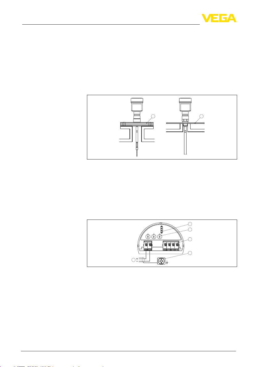
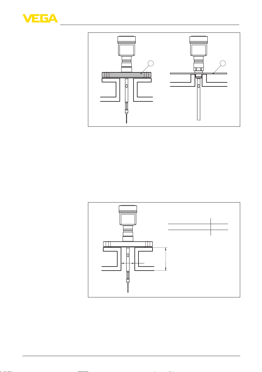
1. Distance from the metallic vessel wall > 300 mm. Distance from non-metallic vessel wall > 500 mm. The probe must not touch any installations or the vessel wall.

2. In non-metallic vessels, place a metal sheet beneath the process tting.

1 2

Fig. 1: Installation in non-metallic vessel

1 Flange 2 Metal sheet

3. If necessary, fasten probe end.

For further information see chapter "Mounting".

1. Make sure that the power supply corresponds to the specications on the type label.

2. Connect the instrument according to the following illustration

Bus

Set parameters

( )

(-)

678

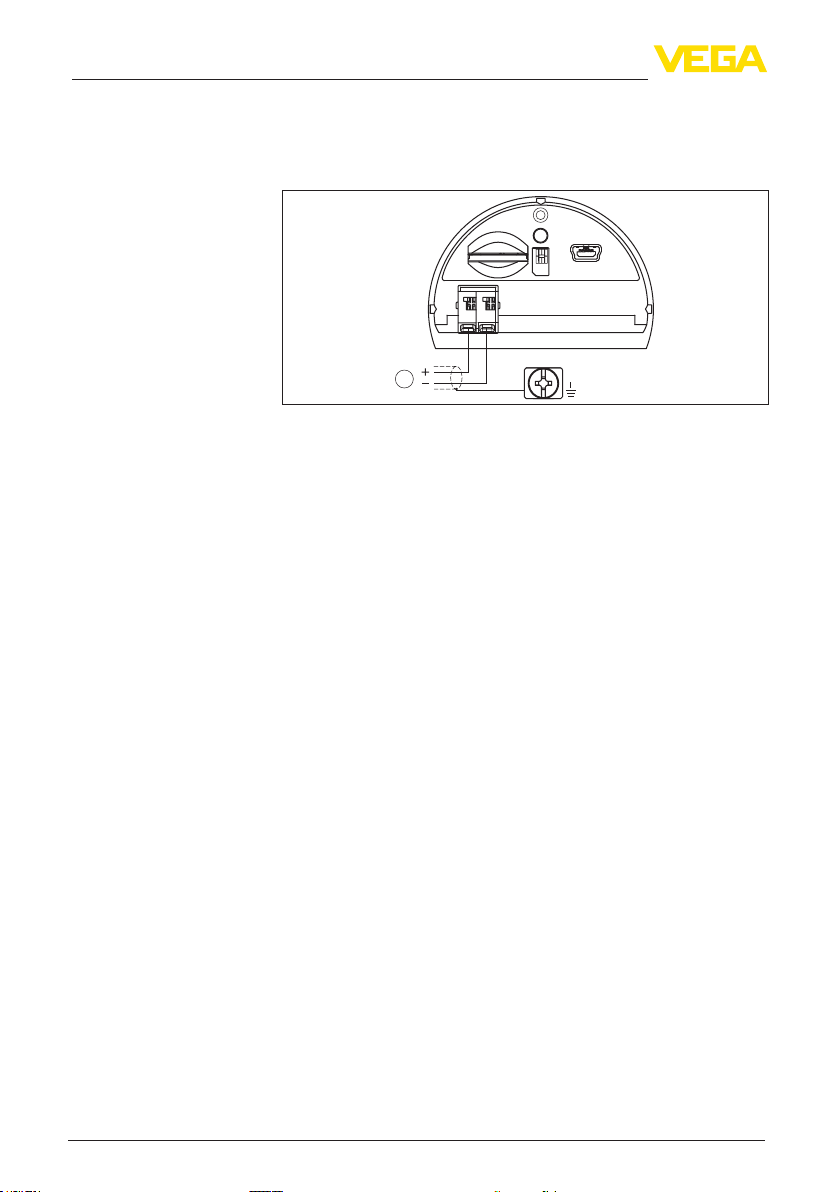
Fig. 2: Electronics and connection compartment, single chamber housing

1 Voltage supply, signal output 2 For display and adjustment module or interface adapter 3 Selection switch for bus address 4 For external display and adjustment unit 5 Ground terminal for connection of the cable screen

For further information see chapter "Connecting to power supply".

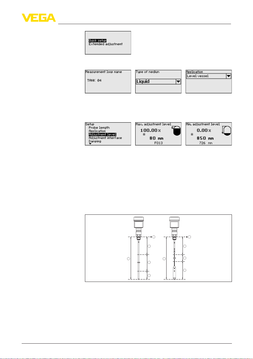
For standard applications we recommend selecting the "Quick setup" in the display and adjustment module.

VEGAFLEX 81 • Probus PA

44217-EN-130910

Quick start

1. In this menu item you can select the application. You can choose between level and interface measurement.

2. In the menu item "Medium - Dielectric constant" you can dene the type of medium (medium).

3. Carry out the adjustment in the menu items "Min. adjustment" and "Max. adjustment".

4. A "Linearization" is recommended for all vessels in which the vessel volume does not increase linearly with the level - e.g. in a horizontal cylindrical or spherical tank. Activate the appropriate curve.

5. A "False signal suppression" detects, marks and saves the false signals so that they are no longer taken into account for level measurement. We generally recommend a false signal suppression.

Parameterization example

44217-EN-130910

VEGAFLEX 81 • Probus PA

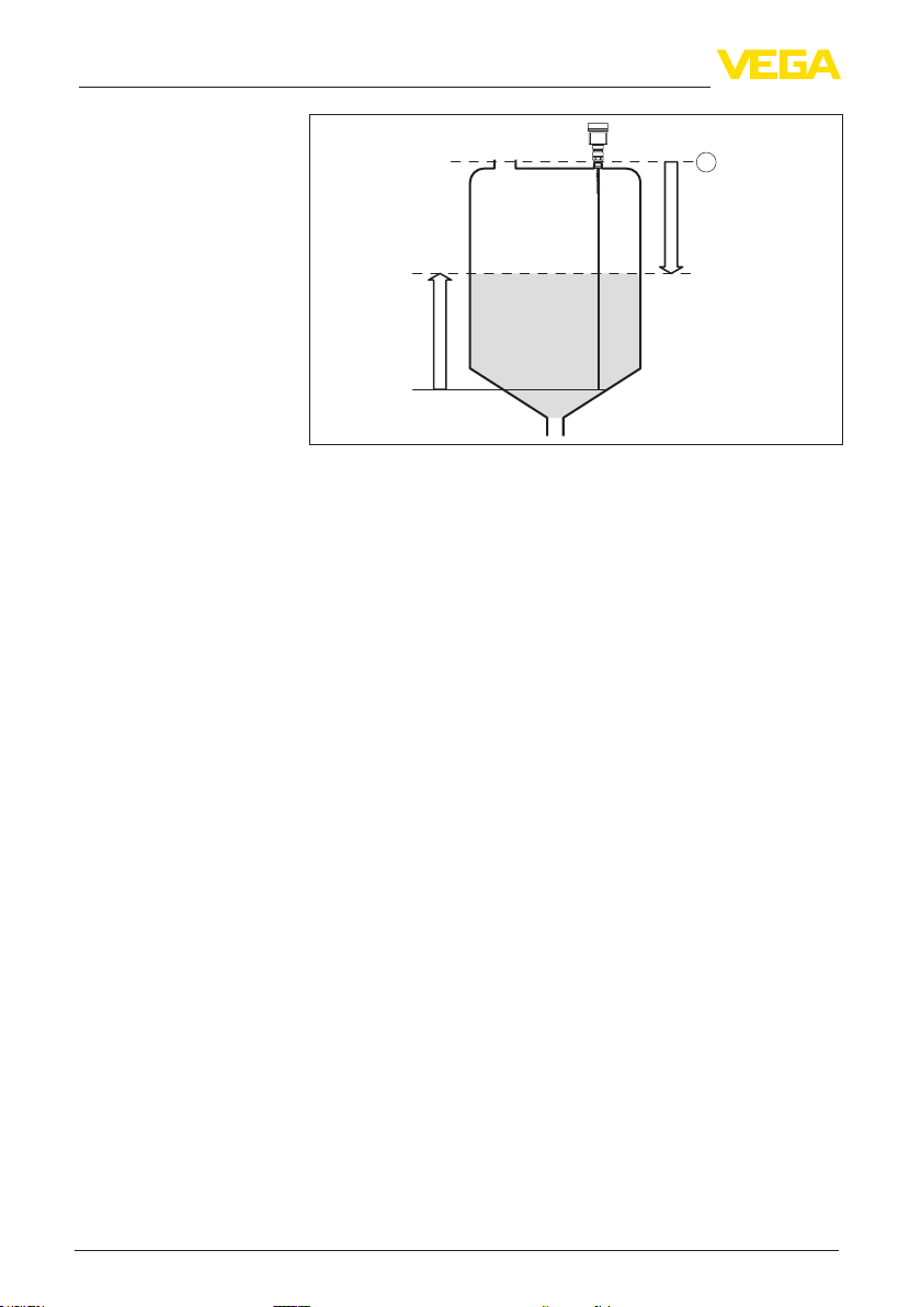
The sensor measures the distance from the sensor (reference plane) to the product surface. See also chapter "Parameter adjustment".

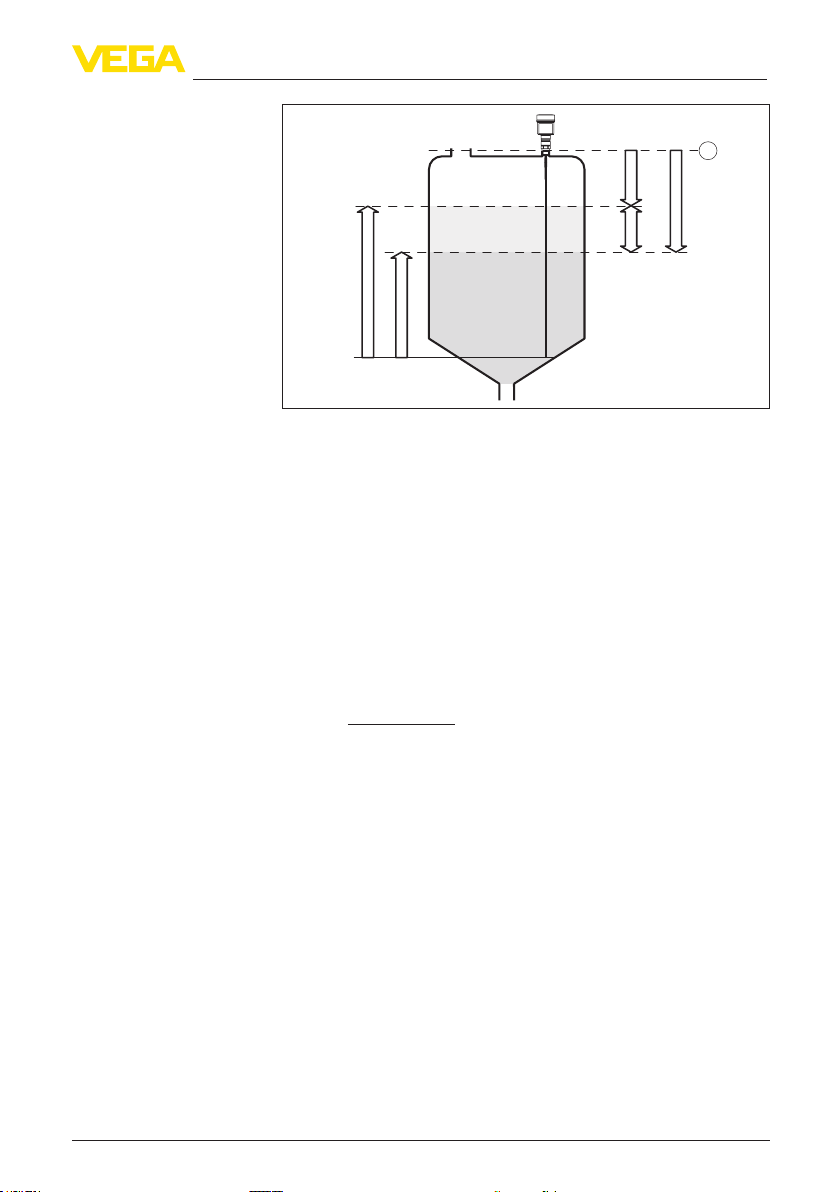
Fig. 3: Measuring ranges - VEGAFLEX 81

1 Reference plane 2 Probe length L 3 Measuring range (default setting refers to the measuring range in water) 4 Upper dead band (in this area no measurement is possible) 5 Lower dead band (in this area no measurement is possible)

For this adjustment, the distance is entered when the vessel is full and nearly empty. If these values are not known, an adjustment with other distances, for example, 10 % and 90 % is also possible. Starting

Quick start

Further steps

point for these distance specications is always the seal surface of the thread or ange.

1. In the menu "Additional settings", menu item "Damping" you can adjust the requested damping of the output signal.

2. Select the parameter of the current output and the output characteristics in the menu item "Current output".

44217-EN-130910

VEGAFLEX 81 • Probus PA

Contents

1 About this document

1.1 Function ........................................................................................................................... 7

1.2 Target group ..................................................................................................................... 7

1.3 Symbolism used ............................................................................................................... 7

2 For your safety

2.1 Authorised personnel ....................................................................................................... 8

2.2 Appropriate use ................................................................................................................ 8

2.3 Warning about incorrect use ............................................................................................. 8

2.4 General safety instructions ............................................................................................... 8

2.5 CE conformity ................................................................................................................... 8

2.6 NAMUR recommendations .............................................................................................. 9

2.7 Environmental instructions ............................................................................................... 9

3 Product description

3.1 Conguration .................................................................................................................. 10

3.2 Principle of operation...................................................................................................... 11

3.3 Packaging, transport and storage ................................................................................... 14

3.4 Accessories and replacement parts ............................................................................... 14

4 Mounting

4.1 General instructions ....................................................................................................... 17

4.2 Mounting instructions ..................................................................................................... 17

5 Connecting to power supply

5.1 Preparing the connection ............................................................................................... 24

5.2 Connecting ..................................................................................................................... 24

5.3 Wiring plan, single chamber housing.............................................................................. 26

5.4 Wiring plan, double chamber housing ............................................................................ 26

5.5 Wiring plan, Ex-d-ia double chamber housing ................................................................ 28

5.6 Wiring plan - version IP 66/IP 68, 1 bar ........................................................................... 29

5.7 Supplementary electronics ............................................................................................. 30

5.8 Set instrument address .................................................................................................. 30

5.9 Switch-on phase............................................................................................................. 31

6 Set up with the display and adjustment module

6.1 Insert display and adjustment module ............................................................................ 32

6.2 Adjustment system ......................................................................................................... 33

6.3 Parameter adjustment - Quick setup .............................................................................. 34

6.4 Parameter adjustment - Extended adjustment................................................................ 37

6.5 Saving the parameter adjustment data ........................................................................... 55

7 Setup with PACTware

7.1 Connect the PC .............................................................................................................. 57

7.2 Parameter adjustment with PACTware ............................................................................ 57

7.3 Set up with the quick setup ............................................................................................. 58

7.4 Saving the parameter adjustment data ........................................................................... 63

8 Set up with other systems

8.1 DD adjustment programs ............................................................................................... 64

9 Diagnostics and service

9.1 Maintenance .................................................................................................................. 65

44217-EN-130910

VEGAFLEX 81 • Probus PA

Contents

9.2 Diagnosis memory ......................................................................................................... 65

9.3 Status messages ............................................................................................................ 66

9.4 Rectify faults ................................................................................................................... 70

9.5 Exchanging the electronics module ................................................................................ 75

9.6 Exchanging the cable/rod ............................................................................................... 75

9.7 Software update ............................................................................................................. 77

9.8 How to proceed in case of repair .................................................................................... 78

10 Dismounting

10.1 Dismounting steps.......................................................................................................... 79

10.2 Disposal ......................................................................................................................... 79

11 Supplement

11.1 Technical data ................................................................................................................ 80

11.2 Communication Probus PA ........................................................................................... 90

11.3 Dimensions .................................................................................................................... 95

44217-EN-130910

Safety instructions for Ex areas

Please note the Ex-specic safety information for installation and operation in Ex areas. These safety instructions are part of the operating instructions manual and come with the Ex-approved instruments.

Editing status: 2013-07-24

VEGAFLEX 81 • Probus PA

1 About this document

1.1 Function

This operating instructions manual provides all the information you need for mounting, connection and setup as well as important instructions for maintenance and fault rectication. Please read this information before putting the instrument into operation and keep this manual accessible in the immediate vicinity of the device.

1.2 Target group

This operating instructions manual is directed to trained specialist personnel. The contents of this manual should be made available to these personnel and put into practice by them.

1.3 Symbolism used

Information, tip, note

This symbol indicates helpful additional information.

Caution: If this warning is ignored, faults or malfunctions can result. Warning: If this warning is ignored, injury to persons and/or serious

damage to the instrument can result. Danger: If this warning is ignored, serious injury to persons and/or

destruction of the instrument can result.

Ex applications

This symbol indicates special instructions for Ex applications.

List

•

The dot set in front indicates a list with no implied sequence.

Action

→

This arrow indicates a single action.

1 Sequence of actions

Numbers set in front indicate successive steps in a procedure.

Battery disposal

This symbol indicates special information about the disposal of batteries and accumulators.

44217-EN-130910

VEGAFLEX 81 • Probus PA

2 For your safety

2.1 Authorised personnel

All operations described in this operating instructions manual must be carried out only by trained specialist personnel authorised by the plant operator.

During work on and with the device the required personal protective equipment must always be worn.

2.2 Appropriate use

VEGAFLEX 81 is a sensor for continuous level measurement. You can nd detailed information on the application range in chapter

"Product description". Operational reliability is ensured only if the instrument is properly

used according to the specications in the operating instructions manual as well as possible supplementary instructions.

2.3 Warning about incorrect use

Inappropriate or incorrect use of the instrument can give rise to application-specic hazards, e.g. vessel overll or damage to system components through incorrect mounting or adjustment.

2.4 General safety instructions

This is a state-of-the-art instrument complying with all prevailing regulations and guidelines. The instrument must only be operated in a technically awless and reliable condition. The operator is responsible for the trouble-free operation of the instrument.

During the entire duration of use, the user is obliged to determine the compliance of the necessary occupational safety measures with the current valid rules and regulations and also take note of new regulations.

The safety instructions in this operating instructions manual, the national installation standards as well as the valid safety regulations and accident prevention rules must be observed by the user.

For safety and warranty reasons, any invasive work on the device beyond that described in the operating instructions manual may be carried out only by personnel authorised by the manufacturer. Arbitrary conversions or modications are explicitly forbidden.

The safety approval markings and safety tips on the device must also be observed.

2.5 CE conformity

The device fullls the legal requirements of the applicable EC guidelines. By axing the CE marking, we conrm successful testing of the product.

You can nd the CE Certicate of Conformity in the download section of our homepage.

VEGAFLEX 81 • Probus PA

44217-EN-130910

2 For your safety

Electromagnetic compatibility

Instruments with plastic housing as well as in four-wire or Ex-d-ia version are designed for use in an industrial environment. Nevertheless, electromagnetic interference from electrical conductors and radiated emissions must be taken into account, as is usual with a class A instrument according to EN 61326-1. If the instrument is used in a dierent environment, the electromagnetic compatibility to other instruments must be ensured by suitable measures.

2.6 NAMUR recommendations

NAMUR is the automation technology user association in the process industry in Germany. The published NAMUR recommendations are accepted as the standard in eld instrumentation.

The device fullls the requirements of the following NAMUR recom-

mendations:

NE 21 – Electromagnetic compatibility of equipment

•

NE 43 – Signal level for malfunction information from measuring

•

transducers

NE 53 – Compatibility of eld devices and display/adjustment

•

components

NE 107 – Self-monitoring and diagnosis of eld devices

•

For further information see www.namur.de.

2.7 Environmental instructions

Protection of the environment is one of our most important duties. That is why we have introduced an environment management system with the goal of continuously improving company environmental protection. The environment management system is certied according to DIN EN ISO 14001.

Please help us fulll this obligation by observing the environmental instructions in this manual:

Chapter "Packaging, transport and storage"

•

Chapter "Disposal"

•

44217-EN-130910

VEGAFLEX 81 • Probus PA

3 Product description

Type plate

3 Product description

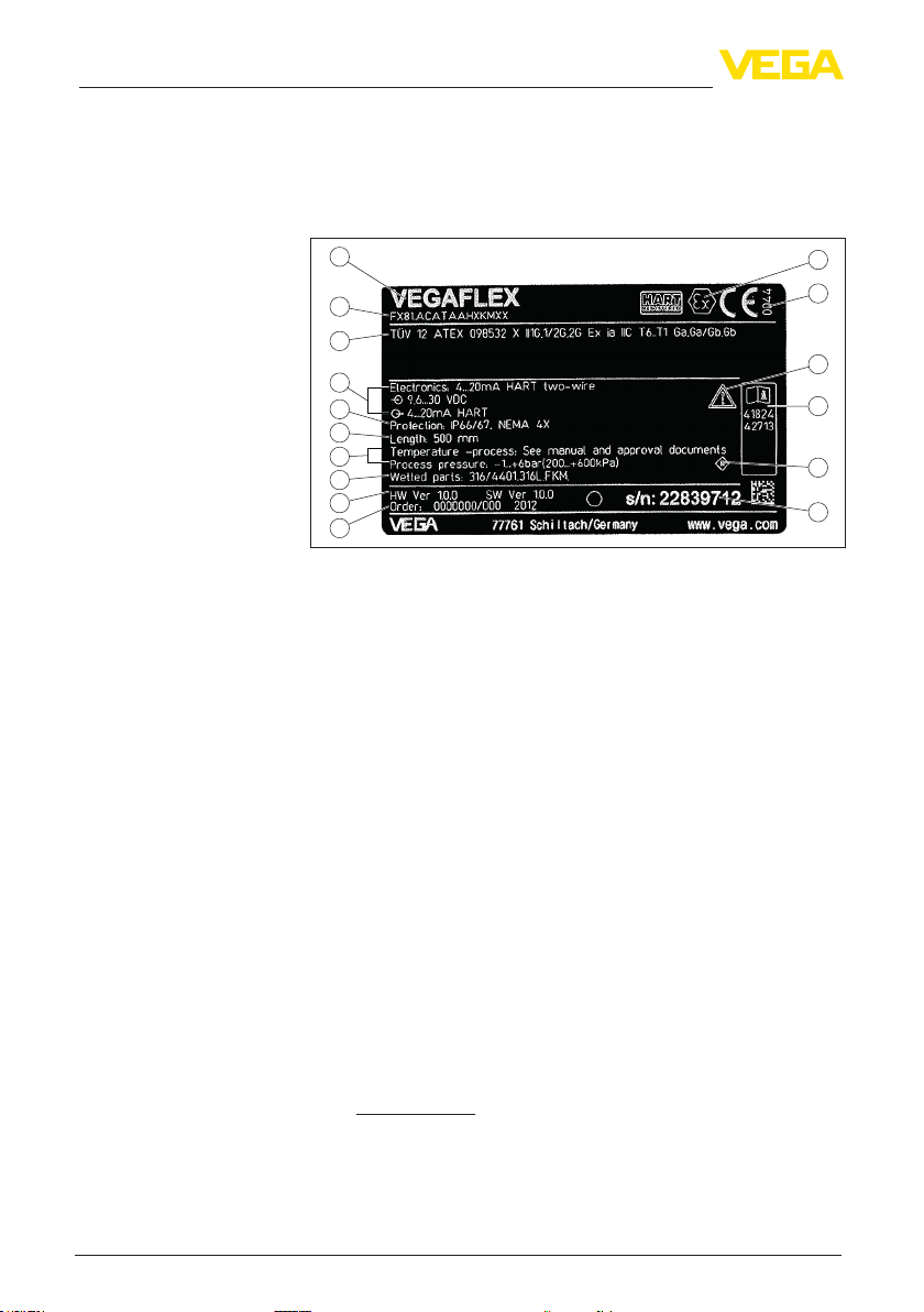
3.1 Conguration

The nameplate contains the most important data for identication and use of the instrument:

4 5

7 8 9

Fig. 4: Layout of the type label (example)

1 Instrument type 2 Product code 3 Approvals 4 Power supply and signal output, electronics 5 Protection rating 6 Probe length 7 Process and ambient temperature, process pressure 8 Material, wetted parts 9 Hardware and software version 10 Order number 11 Serial number of the instrument 12 Symbol of the device protection class 13 ID numbers, instrument documentation 14 Reminder to observe the instrument documentation

15 NotiedauthorityforCEmarking

16 Approval directives

Serial number

The type label contains the serial number of the instruments. Hence you can nd the following data on our homepage:

Product code of the instrument (HTML)

•

Delivery date (HTML)

•

Order-specic instrument features (HTML)

•

Operating instructions at the time of shipment (PDF)

•

Order-specic sensor data for an electronics exchange (XML)

•

Test certicate pressure transmitters (PDF)

•

Go to www.vega.com, "VEGA Tools" and "Serial number search".

As an alternative, you can nd the data via your Smartphone:

Download the smartphone app "VEGA Tools" from the "Apple App

•

Store" or the "Google Play Store" Scan the Data Matrix code on the type label of the instrument or

•

Enter the serial number manually in the app

•

VEGAFLEX 81 • Probus PA

44217-EN-130910

3 Product description

Scope of this operating instructions manual

Versions

Scope of delivery

Application area

This operating instructions manual applies to the following instrument

versions:

Hardware from 1.0.0

•

Software from 1.0.0

•

Only for instrument versions without SIL qualication

•

This electronics version can be determined via the product code on the type label as well as on the electronics.

Standard electronics: Type FX80PA.-

•

The scope of delivery encompasses:

Sensor

•

Documentation

•

– this operating instructions manual – Test certicate measuring accuracy (optional) – Operating instructions manual "Display and adjustment mod-

ule" (optional)

– Supplementary instructions "GSM/GPRS radio module"

(optional)

– Supplementary instructions manual "Heating for display and

adjustment module" (optional)

– Supplementary instructions manual "Plug connector for con-

tinuously measuring sensors" (optional)

– Ex-specic "Safety instructions" (with Ex versions) – if necessary, further certicates

3.2 Principle of operation

The VEGAFLEX 81 is a level sensor with cable or rod probe for continuous level or interface measurement, suitable for applications in liquids.

Functional principle level measurement

44217-EN-130910

VEGAFLEX 81 • Probus PA

High frequency microwave pulses are guided along a steel cable or a rod. Upon reaching the product surface, the microwave pulses are reected. The running time is evaluated by the instrument and outputted as level.

3 Product description

Fig. 5: Level measurement

1 Sensorreferenceplane(sealsurfaceoftheprocesstting)

d Distance to the interface h Height - Level

Probe end tracking

To increase sensitivity, the probe is equipped with probe end tracking. In products with a low dielectric constant, this function is very helpful. This is the case, for example, in plastic granules, packing chips or in vessels with uidized products.

Between a dielectric constant of 1.5 and 3, the function switches on, if required. As soon as the level echo can no longer be detected, probe end tracking is automatically activated. The measurement is continued with the last calculated dielectric constant.

The accuracy thus depends on the stability of the dielectric constant. If you measure a medium with a dielectric constant below 1.5, probe

end tracking is always active. In this case, you have to enter the dielectric constant of the medium. A stable dielectric constant is very important here.

Functional principle - interface measurement

High frequency microwave impulses are guided along a steel cable or rod. Upon reaching the product surface, a part of the microwave impulses is reected. The other part passes through the upper product and is reected by the interface. The running times to the two product layers are processed by the instrument.

44217-EN-130910

VEGAFLEX 81 • Probus PA

3 Product description

Prerequisites for interface measurement

Fig. 6: Interface measurement

1 Sensorreferenceplane(sealsurfaceoftheprocesstting)

d1 Distance to the interface d2 Distance to the level TS Thickness of the upper medium (d1 - d2) h1 Height - Interface h2 Height - Level L1 Lower medium L2 Upper medium L3 Gas phase

Upper medium (L2)

The upper medium must not be conductive

•

The dielectric constant of the upper medium or the actual distance

•

to the interface must be known (input required). Min. dielectric constant: 1.6. You can nd a list of dielectric constants on our home page: www.vega.com. The composition of the upper medium must be stable, no varying

•

products or mixtures The upper medium must be homogeneous, no stratications

•

within the medium

Min. thickness of the upper medium 50 mm (1.97 in)

•

Clear separation from the lower medium, emulsion phase or detri-

•

tus layer max. 50 mm (1.97 in) If possible, no foam on the surface

•

44217-EN-130910

VEGAFLEX 81 • Probus PA

Lower medium (L1)

The dielectric constant must be 10 higher than the dielectric

•

constant of the upper medium, preferably electrically conductive. Example: upper medium dielectric constant 2, lower medium at least dielectric constant 12.

Gas phase (L3)

Air or gas mixture

•

Gas phase - dependent on the application, gas pahse does not

•

always exist (d2 = 0)

3 Product description

Output signal

Packaging

Transport

Transport inspection

Storage

Storage and transport temperature

The instrument is always preset to the application "Level measurement".

For the interface measurement, you can select the requested output signal with the setup.

3.3 Packaging, transport and storage

Your instrument was protected by packaging during transport. Its

capacity to handle normal loads during transport is assured by a test based on ISO 4180.

The packaging of standard instruments consists of environmentfriendly, recyclable cardboard. For special versions, PE foam or PE foil is also used. Dispose of the packaging material via specialised recycling companies.

Transport must be carried out in due consideration of the notes on the

transport packaging. Nonobservance of these instructions can cause damage to the device.

The delivery must be checked for completeness and possible transit

damage immediately at receipt. Ascertained transit damage or concealed defects must be appropriately dealt with.

Up to the time of installation, the packages must be left closed and stored according to the orientation and storage markings on the outside.

Unless otherwise indicated, the packages must be stored only under the following conditions:

Not in the open

•

Dry and dust free

•

Not exposed to corrosive media

•

Protected against solar radiation

•

Avoiding mechanical shock and vibration

•

Storage and transport temperature see chapter "Supplement -

•

Technical data - Ambient conditions" Relative humidity 20 … 85 %

•

PLICSCOM

VEGACONNECT

3.4 Accessories and replacement parts

The display and adjustment module PLICSCOM is used for measured

value indication, adjustment and diagnosis. It can be inserted into the sensor or the external display and adjustment unit and removed at any time.

You can nd further information in the operating instructions "Display and adjustment module PLICSCOM" (Document-ID 27835).

The interface adapter VEGACONNECT enables the connection of

communication-capable instruments to the USB interface of a PC. For parameter adjustment of these instruments, the adjustment software PACTware with VEGA-DTM is required.

VEGAFLEX 81 • Probus PA

44217-EN-130910

3 Product description

You can nd further information in the operating instructions "Interface adapter VEGACONNECT" (Document-ID 32628).

VEGADIS 81

PLICSMOBILE T61

Protective cap

Flanges

Electronics module

The VEGADIS 81 is an external display and adjustment unit for VEGA

plics® sensors. For sensors with double chamber housing the interface adapter

"DISADAPT" is also required for VEGADIS 81. You can nd further information in the operating instructions "VE-

GADIS 81" (Document-ID 43814).

The PLICSMOBILE T61 is an external GSM/GPRS radio unit for

transmission of measured values and for remote parameter adjustment of plics® sensors. The adjustment is carried out via PACTware/ DTM by using the integrated USB connection.

You can nd further information in the supplementary instructions "PLICSMOBILE T61" (Document-ID 37700).

The protective cover protects the sensor housing against soiling and

intense heat from solar radiation. You will nd additional information in the supplementary instructions

manual "Protective cover" (Document-ID 34296).

Screwed anges are available in dierent versions according to the following standards: DIN 2501, EN 1092-1, BS 10, ANSI B 16.5, JIS B 2210-1984, GOST 12821-80.

You can nd additional information in the supplementary instructions manual "Flanges according to DIN-EN-ASME-JIS" (Document-ID

31088).

The electronics module VEGAFLEX series 80 is a replacement part

for TDR sensors of VEGAFLEX series 80. There is a dierent version available for each type of signal output.

You can nd further information in the operating instructions manual "Electronics module VEGAFLEX series 80".

Display and adjustment module with heating

Rod extension

44217-EN-130910

VEGAFLEX 81 • Probus PA

The display and adjustment module can be optionally replaced by a

display and adjustment module with heating function. You can use this display and adjustment module in an ambient tem-

perature range of -40 … +70 °C. You can nd further information in the operating instructions "Display

and adjustment module with heating" (Document-ID 31708).

If you are using an instrument with rod version, you can extend the rod probe individually with curved segments and rod extensions of dierent lengths.

All extensions used must not exceed a total length of 6 m (19.7 ft). The extensions are available in the following lengths:

Rod: ø 12 mm (0.472 in)

Basic segments: 20 … 5900 mm (0.79 … 232 in)

•

3 Product description

Rod segments: 20 … 5900 mm (0.79 … 232 in)

•

Curved segments: 100 x 100 mm (3.94 … 3.94 in)

•

You can nd further information in the operating instructions manual "Rod extension VEGAFLEX series 80".

Bypass tube

Spacer

The combination of a bypass tube and a VEGAFLEX 81 enables con-

tinuous level measurement outside the vessel. The bypass consists of a standpipe which is mounted as a communicating container on the side of the vessel via two process ttings. This kind of mounting ensures that the level in the standpipe and the level in the vessel are the same.

The length and the process ttings can be congured individually. No dierent connection versions available.

You can nd further information in the operating instructions manual "Bypass tube VEGAPASS 81".

If you mount the VEGAFLEX 81 in a bypass tube or standpipe, you have to avoid contact to the bypass tube by using a spacer at the probe end.

You can nd additional information in the operating instructions manual "Centering".

44217-EN-130910

VEGAFLEX 81 • Probus PA

Screwing in

4 Mounting

4.1 General instructions

On instruments with process tting thread, the hexagon must be tightened with a suitable screwdriver. Wrench size see chapter "Dimen- sions".

Warning:

The housing must not be used to screw the instrument in! Applying tightening force can damage internal parts of the housing.

Protection against moisture

Protective caps

Suitability for the process conditions

Protect your instrument further through the following measures against moisture penetration:

Use the recommended cable (see chapter "Connecting to power

•

supply") Tighten the cable gland

•

Loop the connection cable downward in front of the cable gland

•

This applies particularly to:

Outdoor mounting

•

Installations in areas where high humidity is expected (e.g. through

•

cleaning processes) Installations on cooled or heated vessels

•

In the case of instrument housings with self-sealing NPT threads, it is not possible to have the cable entries screwed in at the factory. The openings for the cable glands are therefore covered with red protective caps as transport protection.

Prior to setup you have to replace these protective caps with approved cable glands or close the openings with suitable blind plugs.

The suitable cable glands and blind plugs come with the instrument.

Make sure that all parts of the instrument exposed to the process are suitable for the existing process conditions.

These are mainly:

Active measuring component

•

Process tting

•

Process seal

•

Process conditions are particularly:

Process pressure

•

Process temperature

•

Chemical properties of the medium

•

Abrasion and mechanical inuences

•

You can nd the specications of the process conditions in chapter "Technical data" as well as on the nameplate.

Installation position

44217-EN-130910

VEGAFLEX 81 • Probus PA

4.2 Mounting instructions

Mount VEGAFLEX 81 in such a way that the distance to vessel installations or to the vessel wall is at least 300 mm (12 in). In non-metallic

4 Mounting

vessels, the distance to the vessel wall should be at least 500 mm (19.7 in).

During operation, the probe must not touch any installations or the vessel wall. If necessary, fasten the probe end.

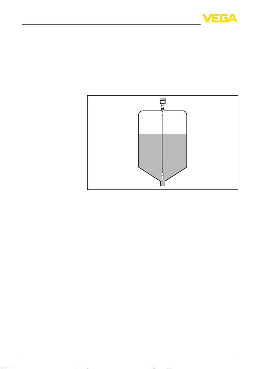
In vessels with conical bottom it can be advantageous to mount the sensor in the center of the vessel, as measurement is then possible nearly down to the lowest point of the bottom. Keep in mind that measurement all the way down to the tip of the probe may not be possible. The exact value of the min. distance (lower dead band) is stated in chapter "Technical data".

Fig. 7: Vessel with conical bottom

Type of vessel

Plastic vessel/Glass vessel

The guided microwave principle requires a metal surface on the process tting. Therefore use in plastic vessels etc. an instrument version with ange (from DN 50) or place a metal sheet (ø > 200 mm/8 in) beneath the process tting when screwing it in.

Make sure that the plate has direct contact with the process tting. When installing rod or cable probes in vessels without metal walls,

e.g. in plastic vessels, the measured value can be inuenced by strong electromagnetic elds (emitted interference according to EN 61326: class A). In this case, use a probe with coaxial version.

44217-EN-130910

VEGAFLEX 81 • Probus PA

1 2

Fig. 8: Installation in non-metallic vessel

1 Flange 2 Metal sheet

4 Mounting

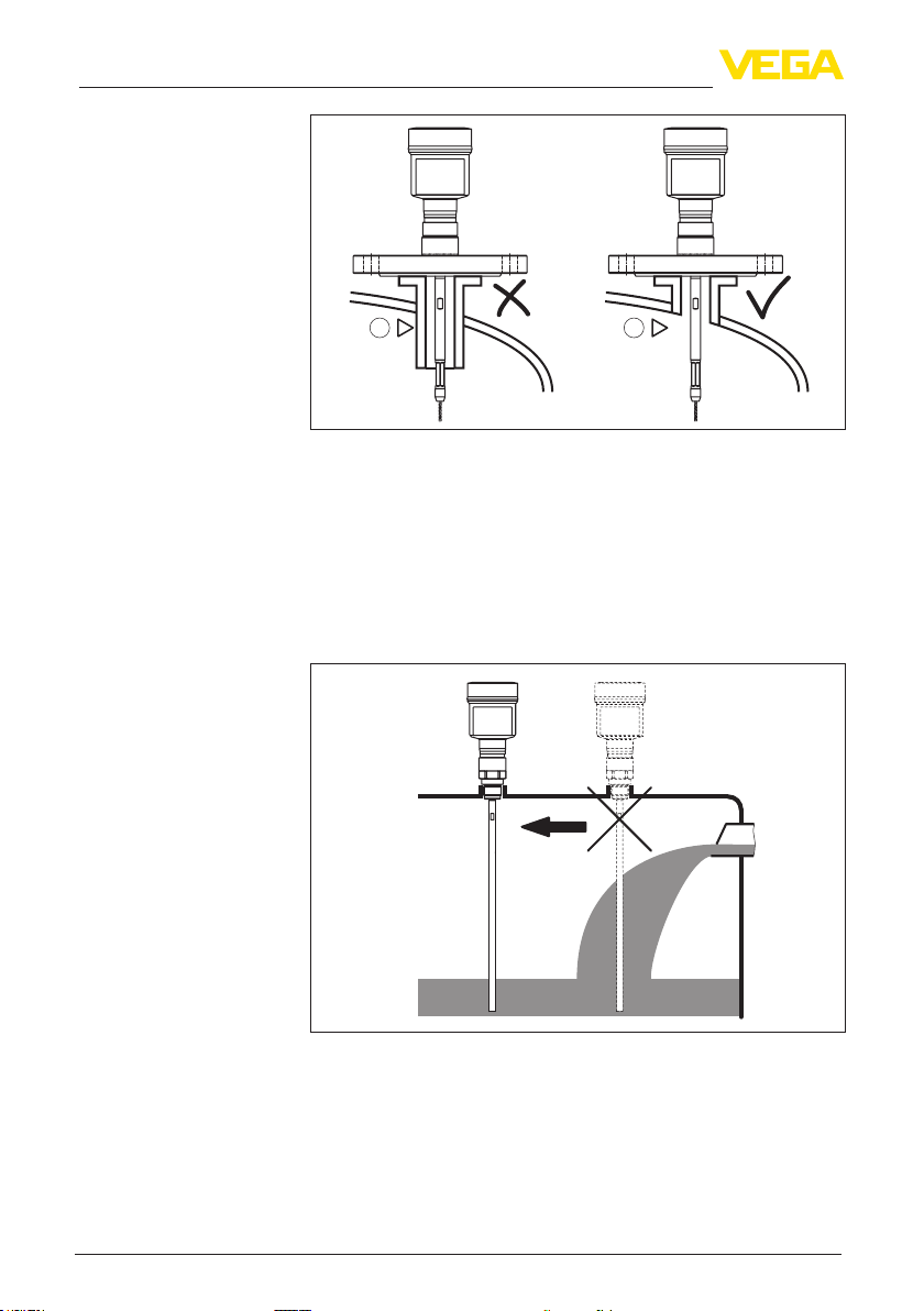
Socket

If possible, avoid sockets. Mount the sensor ush with the vessel top. If this is not possible, use short sockets with small diameter.

Higher sockets or sockets with a bigger diameter can generally be used. They can, however, increase the upper blocking distance (dead band). Check if this is relevant for your measurement.

In such cases, always carry out a false signal suppression after installation. You can nd further information under "Setup procedure".

150

100

Fig. 9: Mounting socket

DN40 ... DN150

> DN150 ... DN200

When welding the socket, make sure that the socket is ush with the vessel top.

44217-EN-130910

VEGAFLEX 81 • Probus PA

4 Mounting

1 2

Fig.10:Socketmustbeinstalledush

1 Unfavourable installation

2 Socketush-optimuminstallation

Welding work

Inowingmedium

Measuring range

Before beginning the welding work, remove the electronics module from the sensor. By doing this, you avoid damage to the electronics through inductive coupling.

Do not mount the instruments in or above the lling stream. Make sure that you detect the product surface, not the inowing product.

Fig.11:Mountingofthesensorwithinowingmedium

The reference plane for the measuring range of the sensors is the

sealing surface of the thread or ange. Keep in mind that a min. distance must be maintained below the refer-

ence plane and possibly also at the end of the probe - measurement in these areas is not possible (dead band). The length of the cable can be used all the way to the end only when measuring conductive

44217-EN-130910

VEGAFLEX 81 • Probus PA

4 Mounting

products. These blocking distances for dierent mediums are listed in chapter "Technical data". Keep in mind for the adjustment that the default setting for the measuring range refers to water.

Pressure

Standpipes or bypass tubes

The process tting must be sealed if there is gauge or low pressure in

the vessel. Before use, check if the seal material is resistant against the measured product and the process temperature.

The max. permissible pressure is specied in chapter "Technical data" or on the type label of the sensor.

Standpipes or bypass tubes are normally metal tubes with a diameter of 30 … 200 mm (1.18 … 7.87 in). In measurement technology, such a tube corresponds to a coax probe. It does not matter if the standpipe is perforated or slotted for better mixing. Lateral inlets in bypass tubes also do not inuence the measurement.

For bypass tubes, select the probe length such that the blocking distance (dead band) of the probe is above or below the lateral lling openings. You can thus measure the complete range of the medium in the bypass tube. When designing the bypass tube, keep the blocking distance of the probe in mind and select the length above the upper lateral lling opening accordingly.

Microwaves can penetrate many plastics. For process technical reasons, plastic standpipes are problematic. If durability is no problem, then we recommend the use of metal standpipes.

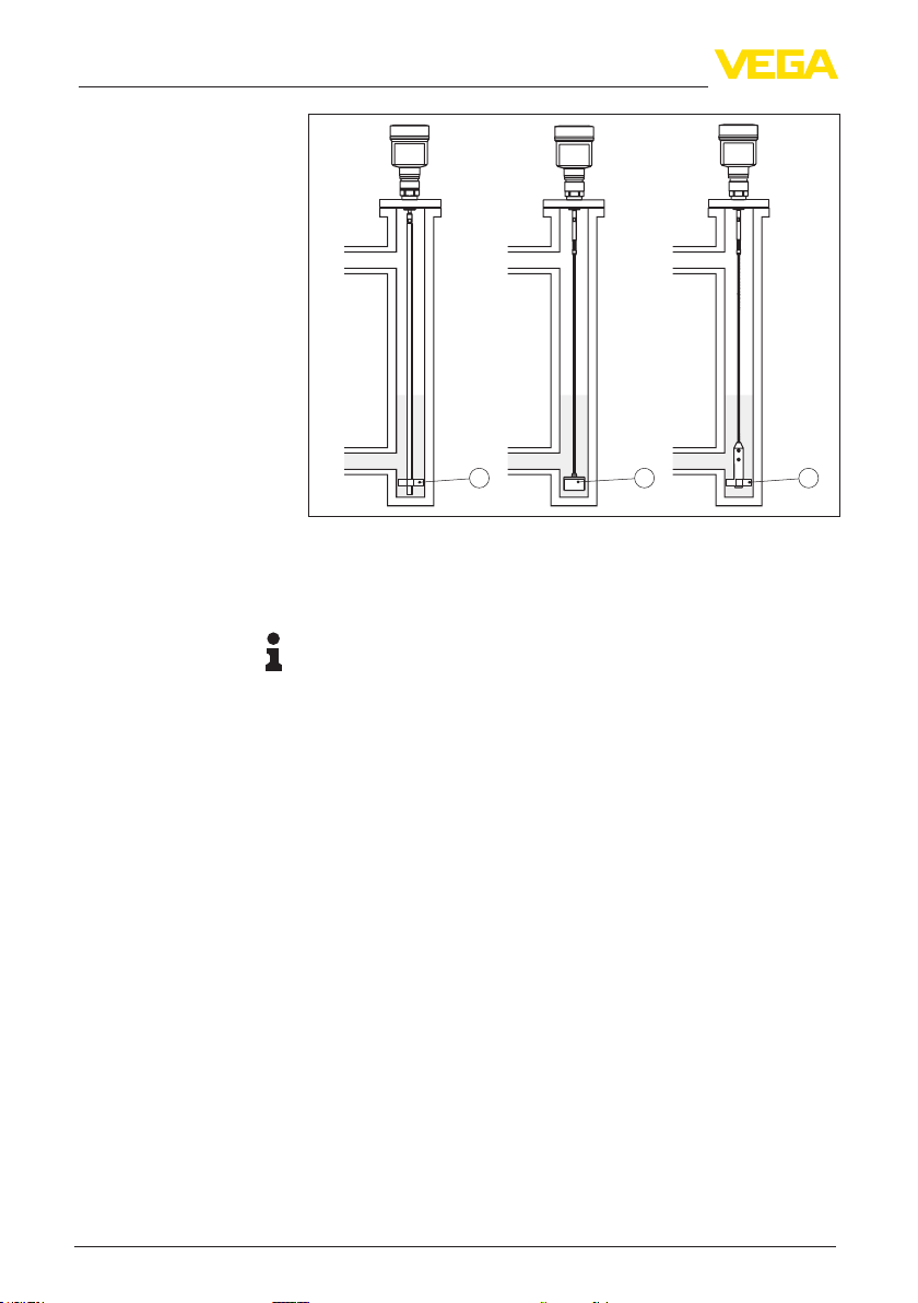
When the VEGAFLEX 81 is used in standpipes or bypass tubes, contact with the tube wall must be avoided. We recommend for this purpose a cable probe with centering weight.

With rod probes, a spacer is generally not required. However, if there is a risk of the rod probe being pressed against the tube wall by inowing medium, you should mount a spacer at the probe end to avoid contact with the tube wall. In the case of cable probes, the cable can be strained.

Keep in mind that buildup can form on the spacers. Strong buildup can inuence the measurement.

44217-EN-130910

VEGAFLEX 81 • Probus PA

4 Mounting

Fasten

Fig. 12: Position of the spacer or centering weight

1 Rod probe with spacer (PEEK) 2 Cable probe with centering weight 3 Spacer (PEEK) on the gravity weight of a cable probe

Note:

Measurement in a standpipe is not recommended for extremely adhesive products.

Instructions for the measurement:

The 100 % point should not be above the upper tube connection

•

to the vessel The 0 % point should not be below the lower tube connection to

•

the vessel A false signal suppression with installed sensor is generally rec-

•

ommended to achieve maximum possible accuracy.

If there is a risk of the cable probe touching the vessel wall during operation due to product movements or agitators, etc., the measuring probe should be securely xed.

In the gravity weight there is an internal thread (M8), e.g. for an eyebolt (optional) - (article no. 2.1512).

Make sure that the probe cable is not completely taut. Avoid tensile loads on the cable.

Avoid undened vessel connections, i.e. the connection must be either grounded reliably or isolated reliably. Any undened change of this requirement can lead to measurement errors.

2 3

44217-EN-130910

VEGAFLEX 81 • Probus PA

4 Mounting

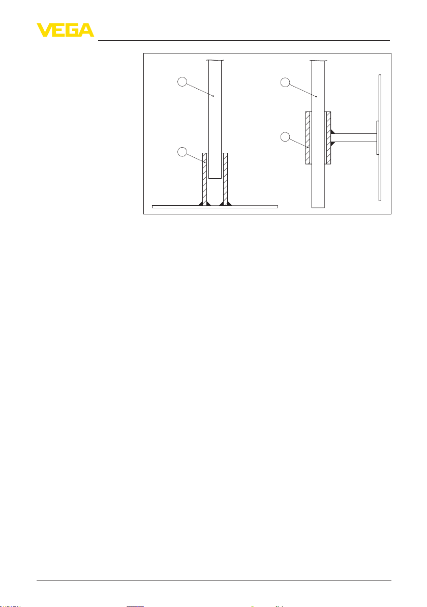
Lateral installation

Fig. 13: Fasten the probe

1 Probe 2 Retaining sleeve

In case of dicult installation conditions, the probe can be also mounted laterally. For this purpose, adapt the rod with rod extensions or bow-shaped segments.

Let the probe length determine automatically by the instrument to compensate the resulting running time changes.

The determine probe length can deviate from the actual probe length when using bow-shaped segments.

If installations such as struts, ladders, etc. exist on the vessel wall, then the probe should have a distance to the vessel wall of at least 300 mm (11.81 in).

You can nd further information in the supplementary instructions of the rod extension.

Rod extension

44217-EN-130910

VEGAFLEX 81 • Probus PA

In case of dicult installation conditions, for example in a socket, the probe can be adapted respectively with a rod extension.

Let the probe length determine automatically by the instrument to compensate the resulting running time changes.

You can nd further information in the supplementary instructions of the rod extension.

5 Connecting to power supply

Safety instructions

5 Connecting to power supply

5.1 Preparing the connection

Always keep in mind the following safety instructions:

Connect only in the complete absence of line voltage

•

If overvoltage surges are expected, overvoltage arresters should

•

be installed

Voltage supply

Connection cable

Cable gland ½ NPT

Cable screening and grounding

The voltage supply is provided by a Probus DP /PA segment coupler.

The voltage supply range can dier depending on the instrument version. You can nd the data for voltage supply in chapter "Technical data".

Connection is made with screened cable according to the Probus specication. Power supply and digital bus signal are carried over the same two-wire connection cable.

Use cable with round cross-section. A cable outer diameter of 5 … 9 mm (0.2 … 0.35 in) ensures the seal eect of the cable gland. If you are using cable with a dierent diameter or cross-section, exchange the seal or use a suitable cable gland.

Please make sure that your installation is carried out according to the Probus specication. In particular, make sure that the termination of the bus is done with appropriate terminating resistors.

You can nd detailed information of the cable specication, installation and topology in the "ProbusPA-UserandInstallationGuide- line" on www.probus.com.

With plastic housing, the NPT cable gland or the Conduit steel tube

must be screwed without grease into the threaded insert. Max. torque for all housings see chapter "Technical data".

Make sure that the cable screen and grounding are carried out according to Fieldbus specication. We recommend to connect the cable screen to ground potential on both ends.

With systems with potential equalisation, connect the cable screen directly to ground potential at the power supply unit, in the connection box and at the sensor. The screen in the sensor must be connected directly to the internal ground terminal. The ground terminal outside on the housing must be connected to the potential equalisation (low impedance).

Connection technology

5.2 Connecting

The voltage supply and signal output are connected via the spring-

loaded terminals in the housing. The connection to the display and adjustment module or to the inter-

face adapter is carried out via contact pins in the housing.

VEGAFLEX 81 • Probus PA

44217-EN-130910

5 Connecting to power supply

Information:

The terminal block is pluggable and can be removed from the electronics. To do this, lift the terminal block with a small screwdriver and pull it out. When reinserting the terminal block, you should hear it snap in.

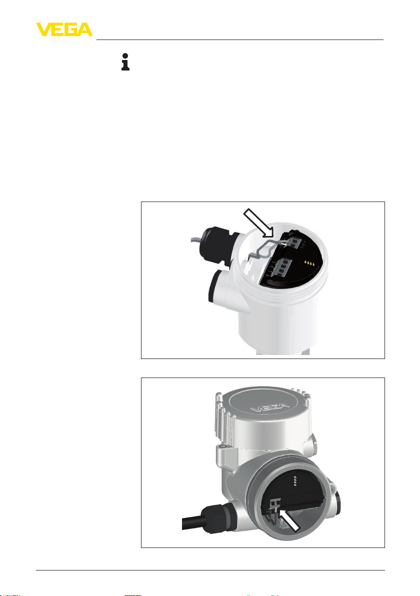
Connection procedure

Proceed as follows:

1. Unscrew the housing cover

2. If a display and adjustment module is installed, remove it by turning it slightly to the left.

3. Loosen compression nut of the cable entry

4. Remove approx. 10 cm (4 in) of the cable mantle, strip approx. 1 cm (0.4 in) of insulation from the ends of the individual wires

5. Insert the cable into the sensor through the cable entry

Fig. 14: Connection steps 5 and 6 - Single chamber housing

44217-EN-130910

VEGAFLEX 81 • Probus PA

Fig. 15: Connection steps 5 and 6 - Double chamber housing

5 Connecting to power supply

Electronics and connection compartment

6. Insert the wire ends into the terminals according to the wiring plan

Information:

Solid cores as well as exible cores with wire end sleeves are inserted directly into the terminal openings. In case of exible cores without end sleeves, press the terminal from above with a small screwdriver; the terminal opening is freed. When the screwdriver is released, the terminal closes again.

You can nd further information on the max. wire cross-section under "Technical data/Electromechanical data"

7. Check the hold of the wires in the terminals by lightly pulling on

them

8. Connect the screen to the internal ground terminal, connect the outer ground terminal to potential equalisation

9. Tighten the compression nut of the cable entry. The seal ring must completely encircle the cable

10. Reinsert the display and adjustment module, if one was installed

11. Screw the housing cover back on

The electrical connection is hence nished.

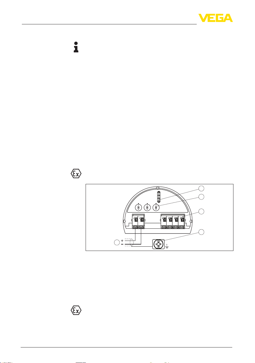
5.3 Wiring plan, single chamber housing

The following illustration applies to the non-Ex, Ex-ia and Ex-d ver-

sion.

Bus

( )

(-)

678

Fig. 16: Electronics and connection compartment, single chamber housing

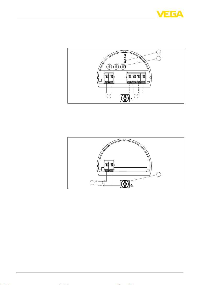
5.4 Wiring plan, double chamber housing

The following illustrations apply to the non-Ex as well as to the Ex-ia

version.

VEGAFLEX 81 • Probus PA

44217-EN-130910

Electronics compartment

Connection compartment

5 Connecting to power supply

Bus

( )

(-)

678

Fig. 17: Electronics compartment, double chamber housing

1 Internal connection to the connection compartment 2 Contact pins for the display and adjustment module or interface adapter 3 Selection switch for bus address

Information:

The connection of an external display and adjustment unit is not possible with this double chamber housing.

Bus

Connection compartment

- Radio module PLICSMOBILE

44217-EN-130910

VEGAFLEX 81 • Probus PA

(-)

( )

Fig. 18: Connection compartment, double chamber housing

1 Voltage supply, signal output 2 For display and adjustment module or interface adapter 3 Ground terminal for connection of the cable screen

SIM-Card

( )

Status

Test

USB

(-)

Fig. 19: Connection compartment radio module PLICSMOBILE

1 Voltage supply

5 Connecting to power supply

Electronics compartment

Connection compartment

You can nd detailed information on connection in the supplementary instructions "PLICSMOBILE GSM/GPRS radio module".

5.5 Wiring plan, Ex-d-ia double chamber housing

Bus

( )

Fig. 20: Electronics compartment, double chamber housing

1 Internal connection to the connection compartment 2 Contact pins for the display and adjustment module or interface adapter 3 Selection switch for bus address 4 Internal connection to the plug connector for external display and adjust-

ment unit (optional)

(-)

678

Bus

( )

(-)

Fig. 21: Connection compartment, double chamber housing Ex d

1 Voltage supply, signal output 2 Ground terminal for connection of the cable screen

VEGAFLEX 81 • Probus PA

44217-EN-130910

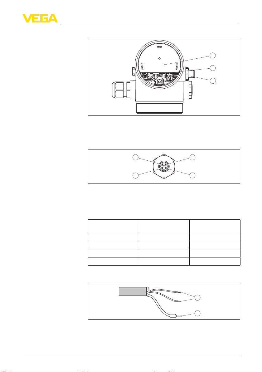
Electronics compartment

Assignment of the plug connector

5 Connecting to power supply

Fig. 22: View to the electronics compartment

1 DIS-ADAPT 2 Internal plug connection 3 Plug connector M12 x 1

Wire assignment, connection cable

44217-EN-130910

VEGAFLEX 81 • Probus PA

Fig. 23: Top view of the plug connector

1 Pin 1 2 Pin 2 3 Pin 3 4 Pin 4

Contact pin Colour connection ca-

ble in the sensor

Pin 1 Brown 5

Pin 2 White 6

Pin 3 Blue 7

Pin 4 Black 8

Terminal, electronics module

5.6 Wiring plan - version IP 66/IP 68, 1 bar

Fig.24:Wireassignmentx-connectedconnectioncable

1 brown (+) and blue (-) to power supply or to the processing system 2 Shielding

5 Connecting to power supply

Supplementary electronics - Radio module PLICSMOBILE

5.7 Supplementary electronics

The radio module PLICSMOBILE is an external GSM/GPRS radio

unit for transmission of measured values and for remote parameter adjustment.

Instrument address

SIM-Card

( )

Status

Test

USB

(-)

Fig. 25: Radio module PLICSMOBILE integrated in the connection compartment

1 Voltage supply

You can nd detailed information on connection in the supplementary instructions "PLICSMOBILE GSM/GPRS radio module".

5.8 Set instrument address

An address must be assigned to each Probus PA instrument. The approved addresses are between 0 and 126. Each address must only be assigned once in the Probus PA network. The sensor is only recognized by the control system if the address is set correctly.

When the instrument is shipped, address 126 is adjusted. This address can be used for function test of the instrument and for connection to a Probus PA network. Then address must be changed to integrate additional instruments.

The address setting is carried out either via:

The address selection switch in the electronics compartment of

•

the instrument (address setting via hardware) The display and adjustment module (address setting via software)

•

PACTware/DTM (address setting via software)

•

Hardware addressing

The hardware addressing is eective if an address <126 is adjusted

with the address selection switches on the instrument. Hence the software addressing is no longer eective, the adjusted hardware address is valid.

44217-EN-130910

VEGAFLEX 81 • Probus PA

5 Connecting to power supply

Bus

( )

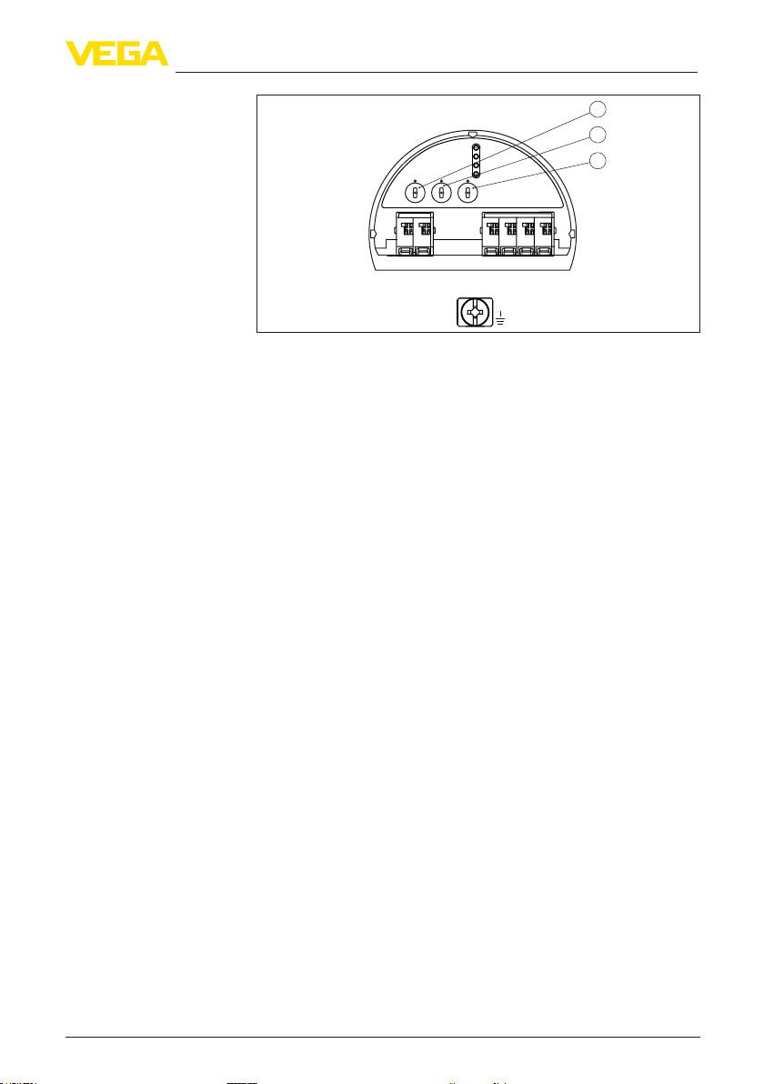
Fig. 26: Address selection switch

1 Addresses <100 (selection 0), addresses >100 (selection 1) 2 Decade of the address (selection 0 to 9) 3 Unit position of the address (selection 0 to 9)

(-)

678

Software addressing

The software addressing is only eective if address 126 or higher is

adjusted on the instrument with the address selection switches. The addressing procedure is described in the operating instructions

manual "Display and adjustment module.

5.9 Switch-on phase

After VEGAFLEX 81 is connected to the bus system, the instrument carries out a self-test for approx. 30 seconds. The following steps are

carried out:

Internal check of the electronics

•

Indication of the instrument type, hardware and software version,

•

measurement loop name on the display or PC Indication of the status message "F 105 Determine measured

•

value" on the display or PC Status byte goes briey to fault value

•

As soon as a plausible measured value is found, it is outputted to the signal cable. The value corresponds to the actual level as well as the settings already carried out, e.g. factory settings.

44217-EN-130910

VEGAFLEX 81 • Probus PA

6 Set up with the display and adjustment module

6 Set up with the display and adjustment

module

6.1 Insert display and adjustment module

The display and adjustment module can be inserted into the sensor and removed any time. Four positions displaced by 90° can be selected. It is not necessary to interrupt the power supply.

Proceed as follows:

1. Unscrew the housing cover

2. Place the display and adjustment module in the requested position onto the electronics and turn to the right until it snaps in

3. Screw housing cover with inspection window tightly back on

Removal is carried out in reverse order. The display and adjustment module is powered by the sensor, an ad-

ditional connection is not necessary.

Fig. 27: Insertion of the display and adjustment module with single chamber housing into the electronics compartment

44217-EN-130910

VEGAFLEX 81 • Probus PA

6 Set up with the display and adjustment module

1 2

Fig. 28: Insertion of the display and adjustment module into the double chamber housing

1 In the electronics compartment 2 In the connection compartment (with Ex-d-ia version not possible)

Note:

If you intend to retrot the instrument with a display and adjustment module for continuous measured value indication, a higher cover with an inspection glass is required.

Key functions

44217-EN-130910

VEGAFLEX 81 • Probus PA

6.2 Adjustment system

Fig. 29: Display and adjustment elements

1 LC display 2 Adjustment keys

[OK] key:

•

– Move to the menu overview

6 Set up with the display and adjustment module

– Conrm selected menu – Edit parameter – Save value

[->] key:

•

– Presentation, change measured value – Select list entry – Select editing position

[+] key:

•

– Change value of the parameter

[ESC] key:

•

– Interrupt input – Jump to next higher menu

Adjustment system

Switch-on phase

Measured value indication

The sensor is adjusted via the four keys of the display and adjust-

ment module. The LC display indicates the individual menu items. The functions of the individual keys are shown in the above illustration. Approx. 10 minutes after the last pressing of a key, an automatic reset to measured value indication is triggered. Any values not conrmed with [OK] will not be saved.

After switching on, the VEGAFLEX 81 carries out a short self-test where the device software is checked.

The output signal transmits a fault signal during the switch-on phase. The following information is displayed on the display and adjustment

module during the startup procedure:

Instrument type

•

Device name

•

Software version (SW-Ver)

•

Hardware version (HW-Ver)

•

With the [->] key you can move between three dierent indication

modes. In the rst view, the selected measured value is displayed in large

digits. In the second view, the selected measured value and a correspond-

ing bar graph presentation are displayed. In the third view, the selected measured value as well as a second

selectable value, e.g. the temperature, are displayed.

Quick setup

44217-EN-130910

6.3 Parameter adjustment - Quick setup

To quickly and easily adapt the sensor to the application, select

the menu item "Quick setup" in the start graphic on the display and adjustment module.

VEGAFLEX 81 • Probus PA

General information

6 Set up with the display and adjustment module

You can nd "Extended adjustment" in the next sub-chapter.

Sensor address

In the rst menu item you have to enter a sensor address. The selection switches on the electronics module are preset to sensor address

126. This means that the sensor address can be changed via the

display and adjustment module.

If you set a sensor address with the selection switches which is lower than 126, the set value is applicable. In such case, the address setting via the display and adjustment module has no eect.

Measurement loop name

In the next menu item you can assign a suitable measurement loop name. You can enter a name with max. 19 characters.

Application

In this menu item, you can select the application. You can choose between level measurement and interface measurement. You can also choose between measurement in a vessel or in a bypass or standpipe.

Level measurement

44217-EN-130910

VEGAFLEX 81 • Probus PA

Medium - dielectric constant

In this menu item, you can dene the type of medium (product).

Max. adjustment

In this menu item, you can enter the max. adjustment for the level. Enter the appropriate distance value in m (corresponding to the

percentage value) for the full vessel. The distance refers to the sensor reference plane (seal surface of the process tting). Keep in mind that the max. level must lie below the dead band.

Min. adjustment

In this menu item, you can enter the min. adjustment for the level. Enter the suitable distance value in m for the empty vessel (e.g.

distance from the ange to the probe end) corresponding to the percentage value. The distance refers tot he sensor reference plane (seal surface of the process tting).

6 Set up with the display and adjustment module

Interface measurement

Dielectric constant - upper medium

In this menu item, you can dene the type of medium (product).

Max. adjustment

In this menu item, you can enter the max. adjustment for the level. Enter the appropriate distance value in m (corresponding to the

percentage value) for the full vessel. The distance refers to the sensor reference plane (seal surface of the process tting). Keep in mind that the max. level must lie below the dead band.

Min. adjustment

In this menu item, you can enter the min. adjustment for the level. Enter the suitable distance value in m for the empty vessel (e.g.

distance from the ange to the probe end) corresponding to the percentage value. The distance refers tot he sensor reference plane (seal surface of the process tting).

Max. adjustment - Interface

Carry out the max. adjustment for the interface. To do this, enter the percentage value and the suitable distance value

in m for the full vessel.

Min. adjustment - Interface

Carry out the min. adjustment for the interface. To do this, enter the percentage value and the suitable distance value

in m for the empty vessel.

Linearization

A linearization is necessary for all vessels in which the vessel volume does not increase linearly with the level - e.g. a horizontal cylindrical or spherical tank, when the indication or output of the volume is required. Corresponding linearization curves are preprogrammed for these vessels. They represent the correlation between the level percentage and vessel volume.

The linearization applies for the measured value indication and the current output. By activating the suitable curve, the percentage vessel volume is displayed correctly.

VEGAFLEX 81 • Probus PA

44217-EN-130910

6 Set up with the display and adjustment module

False signal suppression

High sockets and internal vessel installations cause interfering reections and can inuence the measurement.

A false signal suppression detects, marks and saves these false signals so that they are no longer taken into account for the level and interface measurement. We generally recommend carrying out a false signal suppression to achieve the best possible accuracy. This should be done with the lowest possible level so that all potential interfering reections can be detected.

Enter the actual distance from the sensor to the product surface. All interfering signals in this section are detected by the sensor and

stored. The instrument carries out an automatic false signal suppression

as soon as the probe is uncovered. The false signal suppression is always updated.

AI FB1 Channel

In this menu item you can select the function of the rst Function Block. AI stands for Analog Input.

With this you can adjust the value for the Primary Value (PV). Further settings (SV, TV) must be carried out via PACTware.

Main menu

44217-EN-130910

VEGAFLEX 81 • Probus PA

6.4 Parameter adjustment - Extended adjustment

For technically demanding measurement loops you can carry out extended settings in "Extended adjustment".

The main menu is divided into ve sections with the following func-

tions:

Setup: Settings, e.g. measurement loop name, medium, application, vessel, adjustment, AI FB 1 Channel - Scaling - Damping, device units, false signal suppression, linearization

Display: Language setting, settings for the measured value indication as well as lighting

Diagnosis: Information, for example on the instrument status, pointer, reliability, AI FB 1 simulation, echo curve

6 Set up with the display and adjustment module

Additional adjustments: Sensor address, PIN, date/time, reset,

copy sensor data

Info: Instrument name, hardware and software version, date of manufacture, instrument features

Note:

For optimum adjustment of the measurement, the individual submenu items in the main menu item "Setup" should be selected one after the other and provided with the correct parameters. If possible, go through the items in the given sequence.

The procedure is described below. The following submenu points are available:

The submenu points described below.

Setup - Instrument address

Hardware addressing

Software addressing

Setup - Measurement loop name

An address must be assigned to each Probus PA instrument. Each address may only be assigned once in the Probus PA network. The sensor is only recognized by the control system if the address is set correctly.

The address setting is carried out either via:

The address selection switch in the electronics compartment of

•

the instrument (address setting via hardware) The display and adjustment module (address setting via software)

•

PACTware/DTM (address setting via software)

•

The hardware addressing is eective if an address <126 is set

with the address selection switches on the electronics module of VEGAFLEX 81. Software addressing thus has no eect - only the set hardware address applies.

The software addressing is only eective if address 126 or higher is

adjusted on the instrument with the address selection switches.

Here you can assign a suitable measurement loop name. Push the "OK" key to start the processing. With the "+" key you change the sign and with the "->" key you jump to the next position.

You can enter names with max. 19 characters. The character set

comprises:

44217-EN-130910

VEGAFLEX 81 • Probus PA

6 Set up with the display and adjustment module

Capital letters from A … Z

•

Numbers from 0 … 9

•

Special characters + - / _ blanks

•

Setup - Units

Setup - Units (2)

Setup - Probe length

Setup - Application - Type of medium

In this menu item you select the distance unit and the temperature unit.

With the distance units you can choose between m, mm and ft and with the temperature units betwenn °C, °F and K.

In this menu item, you select the unit of the Secondary Value (SV2).

It can be selected from the distance units such as for example m, mm and ft.

In this menu item you can enter the probe length or have the length determined automatically by the sensor system.

When choosing "Ye s ", then the probe length will be determined automatically. When choosing "No", you can enter the probe length manually.

In this menu item you can select which type of medium you want to measure. You can choose between liquid or bulk solid.

Setup - Application - Application

44217-EN-130910

VEGAFLEX 81 • Probus PA

In this menu item, you can select the application. You can choose between level measurement and interface measurement. You can also choose between measurement in a vessel or in a bypass or standpipe.

6 Set up with the display and adjustment module

Note:

The selection of the application has a considerable inuence on all other menu items. Keep in mind that as you continue with the parameter adjustment, individual menu items are only optionally available.

You have the option of choosing the demonstration mode. This mode is only suitable for test and demonstration purposes. In this mode, the sensor ignores the parameters of the application and reacts immediately to each change.

Setup - Application - Medium, dielectric constant

Setup - Application - Gas phase

Setup - Application - Dielectric constant

In this menu item, you can dene the type of medium (product). This menu item is only available if you have selected level measure-

ment under the menu item "Application".

You can choose between the following medium types:

Dielectric constant

> 10 Water-based liq-

3 … 10 Chemical mix-

< 3 Hydrocarbons Solvents, oils, liquid gas

Type of medium Examples

uids

tures

Acids, alcalis, water

Chlorobenzene, nitro lacquer, aniline, isocyanate, chloroform

This menu item is only available, if you have chosen interface meas-

urement under the menu item "Application". In this menu item you can enter if there is a superimposed gas phase in your application.

Only set the function to "Ye s ", if the gas phase is permanently present.

This menu item is only available if you have selected interface meas-

urement under the menu item "Application". In this menu item you can choose the type of medium of the upper medium.

44217-EN-130910

VEGAFLEX 81 • Probus PA

6 Set up with the display and adjustment module

You can enter the dielectric constant of the upper medium directly or have the value determined by the instrument. To do this you have to enter the measured or known distance to the interface.

Setup - Max. adjustment Level

Setup - Min. adjustment Level

In this menu item you can enter the max. adjustment for the level. With interface measurement this is the maximum total level.

Adjust the requested percentage value with [+] and store with [OK].

Enter the appropriate distance value in m (corresponding to the percentage value) for the full vessel. The distance refers to the sensor reference plane (seal surface of the process tting). Keep in mind that the max. level must lie below the dead band.

In this menu item you can enter the min. adjustment for the level. With interface measurement this is the minimum total level.

Adjust the requested percentage value with [+] and store with [OK].

44217-EN-130910

VEGAFLEX 81 • Probus PA

Enter the suitable distance value in m for the empty vessel (e.g. distance from the ange to the probe end) corresponding to the percentage value. The distance refers tot he sensor reference plane (seal surface of the process tting).

6 Set up with the display and adjustment module

Setup - Max. adjustment Interface

Setup - Min. adjustment Interface

This menu item is only available if you have selected interface meas-

urement under the menu item "Application".

You can accept the adjustment of the level measurement also for the interface measurement. If you select "Yes", the current setting will be displayed.

If you have selected "No", you can enter the adjustment for the interface separately. Enter the requested percentage value.

For the full vessel, enter the distance value in m matching the percentage value.

This menu item is only available if you have selected interface meas-

urement under the menu item "Application". If you have selected "Yes" in the previous menu item (accept adjustment of the level measurement), the current setting will be displayed.

Setup - False signal suppression

If you have selected "No", you can enter the adjustment for the interface measurement separately.

Enter the respective distance value in m for the empty vessel corresponding to the percentage value.

The following circumstances cause interfering reections and can

inuence the measurement:

High sockets

•

Vessel installations such as struts

•

Note:

VEGAFLEX 81 • Probus PA

44217-EN-130910

6 Set up with the display and adjustment module

be done with the lowest possible level so that all potential interfering reections can be detected.

Proceed as follows:

Enter the actual distance from the sensor to the product surface.

All interfering signals in this section are detected by the sensor and stored.

Note:

Check the distance to the product surface, because if an incorrect (too large) value is entered, the existing level will be saved as a false echo. The lling level would then no longer be detectable in this area.

If a false signal suppression has already been created in the sensor, the following menu window appears when selecting "False signal suppression":

Setup - Linearization

44217-EN-130910

VEGAFLEX 81 • Probus PA

The instrument carries out an automatic false signal suppression as soon as the probe is uncovered. The false signal suppression is always updated.

The menu item "Delete" is used to completely delete an already created false signal suppression. This is useful if the saved false signal suppression no longer matches the metrological conditions in the vessel.

The linearization applies to the measured value indication and the current output. By activating the appropriate curve, the volume percentage of the vessel is displayed correctly. If the volume should not be displayed in percent but e.g. in l or kg, a scaling can be also set in the menu item "Display".

6 Set up with the display and adjustment module

Warning:

If a linearization curve is selected, the measuring signal is no longer necessarily linear to the lling height. This must be considered by the user especially when adjusting the switching point on the limit signal transmitter.

In the following, you have to enter the values for your vessel, for example the vessel height and the socket correction.

For non-linear vessel forms, enter the vessel height und the socket correction.

For the vessel height, you have to enter the total height of the vessel. For the socket correction you have to enter the height of the socket

above the upper edge of the vessel. If the socket is lower than the upper edge of the vessel, this value can also be negative.

+ h

- h

Setup - AI FB1

Fig. 30: Vessel height und socket correction value

D Vessel height +h Positive socket correction value

-h Negative socket correction value

44217-EN-130910

Since the adjustment is very comprehensive, the menu points of Function Blocks 1 (FB1) were put together in a submenu.

VEGAFLEX 81 • Probus PA

6 Set up with the display and adjustment module

Setup - AI FB1 - Channel

Setup - AI FB1 - Scaling unit

Setup - AI FB1 - Scaling

In menu item"Channel" you determine which measured value the output refers to.

In menu item "Scaling unit" you dene the scaling variable and the scaling unit for the level value on the display, e.g. volume in l.

In menu item "Scaling" you dene the scaling format on the display and the scaling of the measured level values for 0 % and 100 %.

Level measured value min.

Measured level value max.

Setup - AI FB1 - Damping

Lock/release setup - Adjustment

44217-EN-130910

VEGAFLEX 81 • Probus PA

To damp process-dependent measured value uctuations, you can

set a time of 0 … 999 s in this menu item. The damping applies to the level and interface measurement.

The default setting is a damping of 0 s.

In the menu item "Lock/unlock adjustment", you can protect the sensor parameters against unauthorized modication. The PIN is activated/deactivated permanently.

6 Set up with the display and adjustment module

The following adjustment functions are possible without entering the

PIN:

Select menu items and show data

•

Read data from the sensor into the display and adjustment mod-

•

ule.

Caution:

With active PIN, adjustment via PACTware/DTM as well as other systems is also blocked.

You can change the PIN number under "Additional adjustments - PIN".

Display

Display - Menu language

Display - Displayed value 1

In the main menu point "Display", the individual submenu points should be selected subsequently and provided with the correct parameters to ensure the optimum adjustment of the display options. The procedure is described in the following.

The following submenu points are available:

The submenu points described below.

This menu item enables the setting of the requested national lan-

guage.

In the delivery status, the sensor is set to the ordered national language.

In this menu item, you dene the indication of the measured value on the display. You can display two dierent measured values. In this menu item, you dene measured value 1.

44217-EN-130910

The default setting for the displayed value 1 is "Filling height Level".

Display - Displayed value 2

In this menu item, you dene the indication of the measured value on the display. You can display two dierent measured values. In this menu item, you dene measured value 2.

VEGAFLEX 81 • Probus PA

6 Set up with the display and adjustment module

The default setting for the displayed value 2 is the electronics temperature.

Display - Backlight

Diagnostics - Device status

Diagnostics - Peak values Distance

The optionally integrated background lighting can be adjusted via the

adjustment menu. The function depends on the height of the supply voltage, see "Technical data".

The lighting is switched o in the delivery status.

In this menu item, the device status is displayed.

The respective min. and max. measured value is saved in the sen-

sor. The two values are displayed in the menu item "Peak values, distance".

If you have selected interface measurement under the menu item "Setup - Application", the peak values of the interface measurement are displayed in addition to the peak values of the level measurement.

In another window you can carry out a reset of the two peak values separately.

Diagnostics - Peak values Measurement certainty

44217-EN-130910

VEGAFLEX 81 • Probus PA

The respective min. and max. measured values are saved in the

sensor. The two values are displayed in the menu item "Peak values, measurement certainty".

The measurement can be inuenced by the process conditions. In this menu item, the measurement certainty of the level measurement is displayed as percentage value. The higher the value, the more reliable the measurement. Values > 90 % indicate reliable measurement.

6 Set up with the display and adjustment module

In another window you can carry out a reset of the two peak values separately.

Diagnostics - Peak values Additional

Diagnostics - Echo curve

The respective min. and max. measured values are saved in the

sensor. The values are displayed in the menu item "Peak values Ad- ditional".

This menu item displays the peak values of the electronics temperature as well as the dielectric constant.

In another window you can carry out a reset of the two peak values separately.

The menu item "Echo curve" shows the signal strength of the echoes

over the measuring range in V. The signal strength enables an evaluation of the quality of the measurement.

With the following functions you can zoom part sections of the echo curve.

"X-Zoom": Zoom function for the meas. distance

•

"Y-Zoom": 1, 2, 5 and 10x signal magnication in "V"

•

"Unzoom": Reset the presentation to the nominal measuring range

•

with single magnication

Diagnosis - Simulation

44217-EN-130910

In this menu item you can simulate measured values via the current output. This allows the signal path to be tested, e.g. via downstream indicating instruments or the input card of the control system.

VEGAFLEX 81 • Probus PA

6 Set up with the display and adjustment module

Select the requested simulation size and adjust the requested value.

Caution:

During simulation, the simulated value is outputted as 4 … 20 mA current value and digital HART signal.

Push the [ESC] key to deactivate the simulation.

Information:

The simulation is terminated automatically 60 minutes after the last key has been pushed.

Diagnostics - Echo curve memory

Additional settings - PIN

With the menu item "Setup" the echo curve it is possible to save at

the time of setup. This is generally recommended; for using the Asset Management functions it is necessary. If possible, the curve should be saved with a low level in the vessel.

With this, you can detect signal changes over the operating time. With the adjustment software PACTware and the PC, the high-resolution echo curve can be displayed and used to compare the echo curve of the setup with the actual echo curve.

The function "Echo curve memory" enables storing echo curves of the measurement.

Under the sub-menu item "Echo curve memory" you can store the current echo curve.

Parameter settings for recording the echo curve and the settings of the echo curve itself can be carried out in the adjustment software PACTwa r e.

With the adjustment software PACTware and the PC the high-resolution echo curve can be displayed and used later on to assess the quality of the measurement.

Entering a 4-digit PIN protects the sensor data against unauthorized access and unintentional modication. In this menu item, the PIN is displayed or edited and changed. However, this menu item is only

44217-EN-130910

VEGAFLEX 81 • Probus PA

6 Set up with the display and adjustment module

available if adjustment is enabled in the menu "Lock/Release setup/ adjustment".

In delivery status, the PIN is "0000".

Additional adjustments Date Time

Additional adjustments

- Reset

In this menu item, the internal clock of the sensor is adjusted.

With a reset, certain parameter adjustments carried out by the user

are reset.

The following reset functions are available: Delivery status: Restoring the parameter settings at the time of ship-

ment from the factory incl. the order-specic settings. A created false signal suppression, user-programmable linearization curve as well as the measured value memory will be deleted.

Basic settings: Resetting of the parameter settings incl. special parameters to the default values (presettings) of the respective instrument. Any created false signal suppression or user-programmable linearization curve as well as the measured value memory are deleted.

The following table shows the default values of the instrument. Depending on the instrument version or application, all menu items may not be available or some may be dierently assigned:

Setup

Menu item Default value Modiedvalue

Block adjustment Released

Measurement loop name Sensor

Units Distance unit: mm

Temperature unit: °C

Probe length Length of the probe Ex factory

Type of medium Liquid

Application Level, vessel

VEGAFLEX 81 • Probus PA

44217-EN-130910

6 Set up with the display and adjustment module

Menu item Default value Modiedvalue

Medium, dielectric constant Water-based, > 10

Superimposed gas phase Yes

Dielectric constant, upper medium (TS) 1.5

Tube inner diameter 200 mm

Max. adjustment - Level 100 %

Max. adjustment - Level Distance: 0.000 m(d) - note block-

Min. adjustment - Level 0 %

Min. adjustment - Level Distance: Probe length - take dead

Accept adjustment of the level measurement? Yes

Max. adjustment - Interface 100 %

Max. adjustment - Interface Distance: 0.000 m(d) - note block-

Min. adjustment - Interface 0 %

Min. adjustment - Interface Distance: Probe length - take dead

Integration time - Level 0.0 s

Integration time - Interface 0.0 s

Linearization type Linear

Linearization - Socket correction 0 mm

Linearization - Vessel height Probe length

ing distances

band into account

ing distances

band into account

AI FB1 Tag Descriptor

AI FB1 Channel Primary Value (lin. percent level)

AI FB1 scaling PV Scale (min.) 0 %

AI FB1 scaling PV Scale (max.) 100 %

AI FB1 Lin. Type Linear

AI FB1 Out Scale Unit %

AI FB1 Out Scale Decimal Point #.##

AI FB1 Out Scale (min.) 0 %

AI FB1 Out Scale (max.) 100 %

AI FB1 PV FTime 0 s

AI FB1 Hi Hi Limit 3.402823E+38 %

AI FB1 Hi Limit 3.402823E+38 %

AI FB1 Lo Lo Limit -3.402823E+38 %

AI FB1 Lo Limit -3.402823E+38 %

AI FB1 Hysteresis 0.50 %

44217-EN-130910

VEGAFLEX 81 • Probus PA

6 Set up with the display and adjustment module

Menu item Default value Modiedvalue

AI FB1 Fail Safe Mode (behaviour in case of malfunction)

AI FB1 Fail Safe Value 0.00 %

AI FB1 Target Mode Auto

Last Valid Out Value (last valid measured value)

Display

Menu item Default value Modiedvalue

Language Order-specic

Displayed value 1 Filling height Level

Displayed value 2 Electronics temperature

Backlight Switched o

Diagnostics

Menu item Default value Modiedvalue

Status signals - Function control Switched on

Status signals - Out of specication Switched o

Status signals - Maintenance Switched o

Device memory - Echo curve memory Stopped

Device memory - Measured value memory Started

Device memory - Measured value memory Measured values

Device memory - Measured value memory - Recording in time interval

Device memory - Measured value memory - Recording with measured value dierence

Device memory - Measured value memory - Start with measured value

Device memory - Measured value memory - Stop with measured value

Device memory - Measured value memory - Stop recording when memory is full

Distance level, percentage value level, reliability level, electronics

temperature

3 min.

15 %

Not active

Additional adjustments

Menu item Default value Modiedvalue

PIN 0000

Date Actual date

Time Actual time

Time - Format 24 hours

Probe type Device-specic

VEGAFLEX 81 • Probus PA

44217-EN-130910

6 Set up with the display and adjustment module

Menu item Default value Modiedvalue

AI FB2 Tag Descriptor

AI FB 2 Channel Primary Value (lin. percent level)

AI FB2 scaling PV Scale (min.) 0 %

AI FB2 scaling PV Scale (max.) 100 %

AI FB2 Lin. Type Linear

AI FB2 Out Scale Unit %

AI FB2 Out Scale Decimal Point #.##

AI FB2 Out Scale (min.) 0 %

AI FB2 Out Scale (max.) 100 %

AI FB2 PV FTime 0 s

AI FB2 Hi Hi Limit 3.402823E+38 %

AI FB2 Hi Limit 3.402823E+38 %

AI FB2 Lo Lo Limit -3.402823E+38 %

AI FB2 Lo Limit -3.402823E+38 %

AI FB2 Hysteresis 0.50 %

AI FB2 Fail Safe Mode (behaviour in case of malfunction)

AI FB2 Fail Safe Value 0.00 %

AI FB2 Target Mode Auto

Last Valid Out Value (last valid measured value)

AI FB3 Tag Descriptor

AI FB3 Channel Primary Value (lin. percent level)

AI FB1 scaling PV Scale (min.) 0 %

AI FB3 scaling PV Scale (max.) 100 %

AI FB3 Lin. Type Linear

AI FB3 Out Scale Unit %

AI FB3 Out Scale Decimal Point #.##

AI FB3 Out Scale (min.) 0 %

AI FB3 Out Scale (max.) 100 %

AI FB3 PV FTime 0 s

AI FB3 Hi Hi Limit 3.402823E+38 %

AI FB3 Hi Limit 3.402823E+38 %

AI FB3 Lo Lo Limit -3.402823E+38 %

AI FB3 Lo Limit -3.402823E+38 %

AI FB3 Hysteresis 0.50 %

AI FB3 Fail Safe Mode (behaviour in case of malfunction)

AI FB3 Fail Safe Value 0.00 %

Last Valid Out Value (last valid measured value)

44217-EN-130910

VEGAFLEX 81 • Probus PA

6 Set up with the display and adjustment module

Menu item Default value Modiedvalue

AI FB3 Target Mode Auto

Additional adjustments Copy instrument settings

Additional adjustments Probe type

The instrument settings are copied with this function. The following

functions are available:

Read from sensor: Read data from sensor and store into the

•

display and adjustment module Write into sensor: Store data from the display and adjustment

•

module back to the sensor

The following data or settings for adjustment of the display and adjustment module are saved:

All data of the menu "Setup" and "Display"

•

In the menu "Additional adjustments" the items "Reset, Date/Time"

•

Special parameters

•

The copied data are permanently saved in an EEPROM memory in the display and adjustment module and remain there even in case of power failure. From there, they can be written into one or more sensors or kept as backup for a possible electronics exchange.

Note:

Before the data are stored in the sensor, a check is carried out to determine if the data t the sensor. If the data do not t, a fault signal is triggered or the function is blocked. When data are being written into the sensor, the display shows which instrument type the data originate from and which TAG-no. this sensor had.

In this menu item you can select the type and size of your probe from a list of all possible probes. This is necessary to adapt the electronics optimally to the probe.

Additional adjustments Special parameters

In this menu item you gain access to the protected area where you can enter special parameters. In exceptional cases, individual parameters can be modied in order to adapt the sensor to special requirements.

Change the settings of the special parameters only after having contacted our service sta.

VEGAFLEX 81 • Probus PA

44217-EN-130910

6 Set up with the display and adjustment module

Info - Instrument name

Info - Instrument version

Info - Factory calibration date

Info - Sensor characteristics

In this menu, you read out the instrument name and the instrument serial number:

In this menu item, the hardware and software version of the sensor is displayed.

In this menu item, the date of factory calibration of the sensor as well as the date of the last change of sensor parameters are displayed via the display and adjustment module or via the PC.

In this menu item, the features of the sensor such as approval, process tting, seal, measuring range, electronics, housing and others are displayed.

44217-EN-130910

VEGAFLEX 81 • Probus PA

6.5 Saving the parameter adjustment data

We recommended noting the adjusted data, e.g. in this operating instructions manual, and archiving them afterwards. They are thus available for multiple use or service purposes.

If the instrument is equipped with a display and adjustment module, the data in the sensor can be saved in the display and adjustment module. The procedure is described in the operating instructions manual "Display and adjustment module" in the menu item "Copy sensor data". The data remain there permanently even if the sensor power supply fails.

The following data or settings for adjustment of the display and adjustment module are saved:

All data of the menu "Setup" and "Display"

•

In the menu "Additional adjustments" the items "Sensor-specic

•

units, temperature unit and linearization" The values of the user programmable linearization curve

•

The function can also be used to transfer settings from one instrument to another instrument of the same type. If it is necessary to exchange a sensor, the display and adjustment module is inserted

6 Set up with the display and adjustment module

into the replacement instrument and the data are likewise written into the sensor via the menu item "Copy sensor data".

44217-EN-130910

VEGAFLEX 81 • Probus PA

Via the interface adapter directly on the sensor

Prerequisites

7 Setup with PACTware

7.1 Connect the PC

Fig. 31: Connection of the PC directly to the sensor via the interface adapter

1 USB cable to the PC 2 Interface adapter VEGACONNECT 3 Sensor

7.2 Parameter adjustment with PACTware

For parameter adjustment of the sensor via a Windows PC, the conguration software PACTware and a suitable instrument driver (DTM) according to FDT standard are required. The up-to-date PACTware version as well as all available DTMs are compiled in a DTM Collection. The DTMs can also be integrated into other frame applications according to FDT standard.

Note:

To ensure that all instrument functions are supported, you should always use the latest DTM Collection. Furthermore, not all described functions are included in older rmware versions. You can download the latest instrument software from our homepage. A description of the update procedure is also available in the Internet.

Further setup steps are described in the operating instructions manual "DTM Collection/PACTware" attached to each DTM Collection and which can also be downloaded from the Internet. Detailed descriptions are available in the online help of PACTware and the DTMs.

44217-EN-130910

VEGAFLEX 81 • Probus PA

7 Setup with PACTware

Fig. 32: Example of a DTM view

Standard/Full version

General information

All device DTMs are available as a free-of-charge standard version and as a full version that must be purchased. In the standard version, all functions for complete setup are already included. An assistant for simple project conguration simplies the adjustment considerably. Saving/printing the project as well as import/export functions are also part of the standard version.

In the full version there is also an extended print function for complete project documentation as well as a save function for measured value and echo curves. In addition, there is a tank calculation program as well as a multiviewer for display and analysis of the saved measured value and echo curves.

The standard version is available as a download under www.vega.com/downloads and "Software". The full version is available on CD from the agency serving you.

7.3 Set up with the quick setup

The quick setup is another option for parameter adjustment of the

sensor. It allows fast, convenient adjustment of the most important parameters to adapt the sensor quickly to standard applications. To use it, select the function "Quick setup" in the start screen.

44217-EN-130910

VEGAFLEX 81 • Probus PA

7 Setup with PACTware

Fig. 33: Select quick setup

1 Quick setup 2 Extended adjustment 3 Maintenance

Quick setup

With quick setup you can carry out the parameter adjustment of VEGAFLEX 81 for your application in just a few simple steps. The assistant-driven adjustment includes the basic settings for simple, reliable setup and commissioning.

Information:

If the function is inactive, then possibly no instrument is connected. Check the connection to the instrument.

Extended adjustment

With the extended adjustment, you carry out the parameter adjustment for the instrument via the clear menu structure in the DTM (Device Type Manager). This enables additional and special settings over and above those oered by quick setup.

Maintenance

Under the menu item "Maintenance" you get comprehensive and important support for servicing and maintenance. You can call up diagnostic functions and carry out an electronics exchange or a software update.

Start quick setup

Step 1

Instrumentconguration

44217-EN-130910

VEGAFLEX 81 • Probus PA

Click to the button "Quick setup", to start the assistant-driven adjustment for a simplied and reliable setup.

Device name

Here, you can nd the instrument name. You cannot change this line because the instrument name is unmodiably saved in the instrument.

7 Setup with PACTware

Serial number

Here, you can nd the serial number of your instrument. You cannot change this line because the serial number is unmodiably saved in the instrument.

Measurement loop name

Here you can enter a suitable measurement loop name for your VEGAFLEX 81. You can enter a name with max. 19 characters. You can use capital and small letters as well as numbers. The following special characters are also possible: + - . : , ( ) / < >

Probelengthmodied?

If you have modied the probe length, this must be entered in the selection eld.

If you select "No", then the instrument uses automatically the

•

preset length of the default setting. If you select "Yes ", then you can enter in another eld the modied

•

length of the instrument.

Instrument address

The address setting is carried out either via:

The address selection switch in the electronics compartment of

•

the instrument (address setting via hardware) The display and adjustment module (address setting via software)

•

PACTware/DTM (address setting via software)

•

Hardware addressing - The hardware addressing is eective if an

•

address <126 is set with the address selection switches on the electronics module of VEGAFLEX 81. The software addressing is then no longer eective, only the set hardware address is valid. Software addressing - The software addressing is only eective

•

if address 126 or higher is set on the instrument with the address selection switches.

Probe length L from seal surface

If you have modied the length of the probe, you can enter in this eld the modied probe length. Keep the selected unit in mind.

Determine probe length automatically

If you do not know the probe length, you can have the length of the probe determined automatically. The requirement for this is a probe unrestricted and not covered by the medium.

Click to "Carry out now", to start the automatic length determination.

VEGAFLEX 81 • Probus PA

44217-EN-130910

7 Setup with PACTware

Step 2 Application

Type of medium

Here you can see which type of medium your instrument is suitable for. If this function is inactive, the medium type your instrument is suitable for was already preset.

Information:

In special cases you can change the type of medium. This setting can be changed under "Extended adjustment".

Application

In this eld you can select the application you want to use your instrument for. You have the following selection options:

Level in the vessel

•

Level in the bypass/standpipe

•

Interface in the vessel

•

Interface in the bypass/standpipe

•

Demonstration mode

•

Level measurement: If you select "Level", you can select the properties of the medium in another eld.

Interface measurement: If you select "Interface", the instrument needs more information, such as the distance to the interface, the dielectric constant of the upper medium or whether or not there is a superimposed gas phase.

Demonstration mode: This mode is only suitable for test and demonstration purposes. In this mode, the sensor ignores all parameters and reacts immediately to all measured value changes within the measuring range.

Application - Level measurement

The level measurement refers to the product surface which is the limit to the gas phase.

Liquids

•

– Solvents, oils, LPG - dielectric constant < 3 – Chemical mixtures - dielectric constant 3 … 10 – Water-based - dielectric constant > 10

Bulk solids

•

– Dusts, wood chips - dielectric constant < 1.5 – Granules, dusts, powders - dielectric constant 1.5 … 3 – Cereals, our - dielectric constant > 3

44217-EN-130910

VEGAFLEX 81 • Probus PA

Application - Interface measurement

The interface measurement refers to the phase limit between two liquids. The total level is also available as a measured value.

Superimposed gas phase present

•

– Check if there is a superimposed gas phase in the vessel. This

is always the case if the total level never touches the process tting.

Properties

•

– Here you can enter the dielectric constant of the upper medium – As an alternative you can enter the distance to the interface

7 Setup with PACTware

Step 3 Adjustment

Step 4 Linearization

Step 5 Setting - AI FB1

Adjustment for the level measurement

If you have selected level measurement in the previous menu, then you can enter the values for the min. and max. adjustment. The value to be entered refers to the distance from the sealing surface of the process tting (sensor reference plane) to the surface of the product.

Adjustment for the level and interface measurement

If you have selected interface measurement in the previous menu, then you can enter the values for the min. and max. adjustment of level and interface or accept the values of the level measurement. The entered value refers to the distance from the sealing surface of the process tting (sensor reference plane) to the total level or interface.

Linearization is required if the measured value should be outputted in proportion to the volume and not the level. The linearization acts identically on the level and the interface measurement. You can nd further linearization types in the extended adjustment.

If you have a non-linear vessel, you can select here the respective linearization curve.

Linear

•

Spherical tank

•

Horizontal cylindrical tank

•

You must enter the following vessel dimensions with non-linear conditions:

Height of the socket h

•

Vessel height D

•

In this window you can adjust the output signal. When the function is inactive, you can change the settings via the "Extended adjustment".

Scaling unit

In the menu item "Out Scale Unit (scaling unit)" you dene the scaling unit, for example volume in l for the specied channel (measured value).

Scaling

In the menu items "Out Scale (min.)" and "Out Scale (max.)" you dene the scaling of the measured values for 0 % and 100 %.

Step 6 Sensor optimization

These settings allow you to optimize the sensor. With them you can

compare a sounded distance with the indicated value and correct it, if necessary.

Probe immersed in the liquid (covered)

Select whether or not the probe is immersed in the medium.

Measured distance to the medium

If the probe is immersed in the medium, you can enter here the measured distance to the medium.

VEGAFLEX 81 • Probus PA

44217-EN-130910

7 Setup with PACTware

Displayeddistancecorrect?

Is the displayed distance value correct? If you have the possibility, you can enter here the sounded distance to the medium.

False signal suppression

With this function you can carry out the automatic false signal suppression. We recommend carrying out false signal suppression in any case.

Step 7 Additional settings

When the setup of the instrument is nished, additional settings can

be made. These are various backups and the locking of the instrument against unauthorised or inadvertent adjustment.

Prepareabackupleoftheinstrumentparameteradjustment?

For backup purposes, the current parameter adjustment of the instrument is stored in a le. You can use this le later on to restore the instrument parameter adjustment. The complete data set is downloaded from the device. This procedure can last several minutes.

Createinstrumentdocumentation?

This function is used to print or create a PDF le of the current parameter adjustment. To read the PDF le, you need a suitable program (for example Acrobat Reader). To print or create the PDF le, all data are downloaded from the device. For this function, the full version of the DTM Collection is required. This procedure can last several minutes.

Storeechocurveofthesetupinthesensor?

Have you completed the initial setup of the instrument? In such case, we recommend storing the current signal conditions in the device for later instrument tests and diagnostics.

LockadjustmentwithPINaftersetting?

The instrument is locked with the current PIN. A parameter adjustment is possible only after the PIN is entered again.

7.4 Saving the parameter adjustment data

We recommend documenting or saving the parameter adjustment data via PACTware. That way the data are available for multiple use or service purposes.

44217-EN-130910

VEGAFLEX 81 • Probus PA

8 Set up with other systems

8.1 DD adjustment programs

Device descriptions as Enhanced Device Description (EDD) are available for DD adjustment programs such as, for example, AMS™ and PDM.

The les can be downloaded at www.vega.com/downloads under "Software".

44217-EN-130910

VEGAFLEX 81 • Probus PA

9 Diagnostics and service

9.1 Maintenance

If the device is used correctly, no maintenance is required in normal operation.

9.2 Diagnosis memory

The instrument has several memories which are available for diagnosis purposes. The data remain even with voltage interruption.

Measured value memory

Event memory

Up to 100,000 measured values can be stored in the sensor in a ring memory. Each entry contains date/time as well as the respective measured value. Storable values are for example:

Distance

•

Filling height

•

Percentage value

•

Lin. percent

•

Scaled

•

Current value

•

Meas. reliability

•

Electronics temperature

•

When the instrument is shipped, the measured value memory is active and stores distance, measurement certainty and electronics temperature every 3 minutes.

In "Extended adjustment" you can select the respective measured values.

The requested values and recording conditions are set via a PC with PACTware/DTM or the control system with EDD. Data are thus read out and also reset.

Up to 500 events are automatically stored with a time stamp in the sensor (non-deletable). Each entry contains date/time, event type, event description and value. Event types are for example:

Modication of a parameter

•

Switch-on and switch-o times

•

Status messages (according to NE 107)

•

Error messages (according to NE 107)

•

The data are read out via a PC with PACTware/DTM or the control system with EDD.

Echo curve memory

44217-EN-130910

VEGAFLEX 81 • Probus PA

The echo curves are stored with date and time and the corresponding

echo data. The memory is divided into two sections: Echo curve of the setup: This is used as reference echo curve for

the measurement conditions during setup. Changes in the measurement conditions during operation or buildup on the sensor can thus be recognized. The echo curve of the setup is stored via:

PC with PACTware/DTM

•

Control system with EDD

•

9 Diagnostics and service

Display and adjustment module

•

Further echo curves: Up to 10 echo curves can be stored in a ring buer in this memory section. Further echo curves are stored via:

PC with PACTware/DTM

•

Control system with EDD

•

Display and adjustment module

•

9.3 Status messages

The instrument features self-monitoring and diagnostics according to NE 107 and VDI/VDE 2650. In addition to the status messages in the following tables there are more detailed error messages available under the menu item "Diagnostics" via the display and adjustment module, PACTware/DTM and EDD.

Status messages

The status messages are divided into the following categories:

Failure

•

Function check

•

Out of specication

•

Maintenance requirement

•

and explained by pictographs:

41 2 3

Fig. 34: Pictographs of the status messages

1 Failure - red

2 Outofspecication-yellow

3 Function check - orange 4 Maintenance - blue

Failure: Due to a malfunction in the instrument, a failure message is outputted.

This status message is always active. It cannot be deactivated by the user.

Function check: The instrument is in operation, the measured value is temporarily invalid (for example during simulation).

This status message is inactive by default. It can be activated by the user via PACTware/DTM or EDD.

Outofspecication: The measured value is unstable because the instrument specication is exceeded (e.g. electronics temperature).

This status message is inactive by default. It can be activated by the user via PACTware/DTM or EDD.

Maintenance: Due to external inuences, the instrument function is limited. The measurement is aected, but the measured value is

44217-EN-130910

VEGAFLEX 81 • Probus PA

9 Diagnostics and service

still valid. Plan in maintenance for the instrument because a failure is expected in the near future (e.g. due to buildup).

This status message is inactive by default. It can be activated by the user via PACTware/DTM or EDD.

Failure (failure)

The following table shows the codes and text messages of the status

message "Failure" and provides information on causes as well as corrective measures.

Code

Text message

F013

no meas-

ured value available

F017

Adjustment

span too

small

F025

Error in the

linearization table

F036

No op-

erable software

F040

Error in the

electronics

F080 – General software error – Separate operating

F105

Determine measured

value

F113 Communi-

cation error

Cause Rectication PA DevS-

– Sensor does not

detect an echo during

operation

– Antenna system con-

taminated or defective

– Adjustment not within

specication

– Index markers are not

continuously rising, for examle unlogical value

pairs

– Failed or interrupted

software update

– Hardware defect – Exchanging the elec-

– The instrument is still

in the start phase, the measured value could not yet be determined

– Error in the internal

instrument communication

– Check or correct

installation and/or parameter adjustment

– Clean or exchange

process component or antenna

– Change adjustment

according to the limit values (dierence between min. and max. ≥ 10 mm)

– Check linearization

table

– Delete table/Create

new

– Repeat software

update

– Check electronics

version

– Exchanging the elec-

tronics

– Send instrument for

repair

tronics

– Send instrument for

repair

voltage briey

– Wait for the end of the

switch-on phase

– Duration depending

on the version and

parameter adjustment up to approximately 3 min.

– Separate operating

voltage briey

– Send instrument for

repair

pec

Diagnosis

Bit 0

Bit 1

Bit 2

Bit 3

Bit 4

Bit 5

Bit 6

Bit 7

44217-EN-130910

VEGAFLEX 81 • Probus PA

9 Diagnostics and service

Code

Text message

F125 Unper-

missible electronics

temperature

F260

Error in the

calibration

F261

Error in the conguration

F264 Installa-

tion/Setup

error

F265 Meas-

urement

function disturbed

F267 No execut-

able sensor software

Cause Rectication PA DevS-

– Temperature of the

electronics in the nonspecied section

– Error in the calibra-

tion carried out in the

factory

– Error in the EEPROM

– Error during setup – False signal suppres-

sion faulty

– Error when carrying

out a reset

– Adjustment not within

the vessel height/ measuring range

– Max. measuring range

of the instrument not sucient

– Sensor no longer

carries out a measurement

– Operating voltage

too low

– Sensor cannot start – Exchanging the elec-

– Check ambient tem-

perature

– Isolate electronics – Use instrument with

higher temperature range

– Exchanging the elec-

tronics

– Send instrument for

repair

– Repeat setup – Repeat reset

– Check or correct

installation and/or parameter adjustment

– Use an instrument

with bigger measuring range

– Check operating

voltage

– Carry out a reset – Separate operating

voltage briey

tronics

– Send instrument for

repair

pec

Diagnosis

Bit 8

Bit 9

Bit 10

Bit 11

Bit 12

Function check

Outofspecication

The following table shows the error codes and text messages in the

status message "Function check" and provides information on causes as well as corrective measures.

Code

Text message

C700 Simulation ac-

tive

Cause Rectication

– A simulation is active – Finish simulation

– Wait for the automatic end

after 60 mins.

The following table shows the error codes and text messages in the

status message "Outofspecication" and provides information on causes as well as corrective measures.

VEGAFLEX 81 • Probus PA

44217-EN-130910

9 Diagnostics and service

Maintenance

Code

Text message

S600 Unpermissi-

ble electronics

temperature

S601 Overlling

S602 Level with-

in the search range, compensation echo

S603

Impermissi-

ble operating voltage

Cause Rectication

– Temperature of the pro-

cessing electronics in the non-specied section

– Level echo in the close

range not available

– Compensation echo super-

imposed by medium

– Operating voltage below

specied range

– Check ambient temperature – Isolate electronics – Use instrument with higher

temperature range

– Reduce level – 100 % adjustment: Increase

value

– Check mounting socket – Remove possible interfering

signals in the close range

– Use coaxial probe

– 100 % adjustment: Increase

value

– Check electrical connection – if necessary, increase

operating voltage

The following table shows the error codes and text messages in the

status message "Maintenance" and provides information on causes as well as corrective measures.

Code

Text message

M500

Error in the delivery status

M501

Error in the non-active

linearization table

M502

Error in the event memory

M503 Reliability too

low

Cause Rectication

– With the reset to delivery

status, the data could not be restored

– Hardware error EEPROM – Exchanging the electronics

– Measurement certainty is

too low for a reliable measurement

– Process component or

probe contaminated or defective

– Repeat reset – Load XML le with sensor

data into the sensor

– Send instrument for repair

– Check installation and

process conditions

– Clean or exchange process

component or probe

44217-EN-130910

VEGAFLEX 81 • Probus PA

9 Diagnostics and service

Reaction when malfunctions occur

Procedure for fault recti-

cation

Code

Text message

M504

Error on an device inter-

face

M505

no measured

value available

M506 Installation/

Setup error

M507

Error in the instrument

settings

Cause Rectication

– Hardware defect – Exchanging the electronics

– Sensor does not detect an

echo during operation

– Process component or

probe contaminated or defective

– Error during setup – Check and correct instal-

– Error during setup – Error when carrying out a

reset

– False signal suppression

faulty

– Send instrument for repair

– Check and correct instal-

lation and/or parameter adjustment

– Clean or exchange process

component or probe

lation and/or parameter adjustment

– Check probe length

– Carry out reset and repeat

setup

9.4 Rectify faults

The operator of the system is responsible for taking suitable meas-

ures to rectify faults.

The rst measures are:

Evaluation of fault messages, for example via the display and

•

adjustment module Checking the output signal

•

Treatment of measurement errors

•

Further comprehensive diagnostics options oer a PC with the software PACTware and the suitable DTM. In many cases, the reasons can be determined in this way and faults can be rectied.

Treatment of measurement errors

The below tables show typical examples for application-relevant

measurement errors. There are two measurement errors:

Constant level

•

Filling

•

Emptying

•

The images in column "Error pattern" show the real level with a broken line and the level displayed by the sensor as a continuous line.

VEGAFLEX 81 • Probus PA

44217-EN-130910

Level

time

9 Diagnostics and service

Fig. 35: The broken line 1 shows the real level, the continuous line 2 shows the level displayed by the sensor

Note:

Wherever the sensor displays a constant value, the reason could

•

also be the fault setting of the current output to "Hold value" In case of a too low level indication, the reason could be a line

•

resistance that is too high

Measurement error with constant level

Fault description Error pattern Cause Rectication

1. Measured value shows a too low or too high level

2. Measured value jumps towards 100 %

Level

– Min./max. adjustment not

correct

– Wrong linearization curve – Adapt linearization curve

– Running time error (small

measurement error close to 100 %/serious error close to 0 %)

– Due to the process, the ampli-

tude of the product echo sinks

– A false signal suppression was

not carried out

– Amplitude or position of a

false signal has changed (e.g. buildup); false signal suppression no longer matches

– Adapt min./max. adjustment

– Repeat setup

– Carry out a false signal sup-

pression

– Determine the reason for the

changed false signals, carry out false signal suppression, e.g. with buildup

time

44217-EN-130910

Measurementerrorduringlling

Fault description Error pattern Cause Rectication

3. Measured value remains in the area of the bottom during lling

Level

– Echo from the probe end larger

than the product echo, for example, with products with εr < 2.5 oil-based, solvents, etc.

– Check parameter "Medium"

and "Vessel height", adapt if

necessary

VEGAFLEX 81 • Probus PA

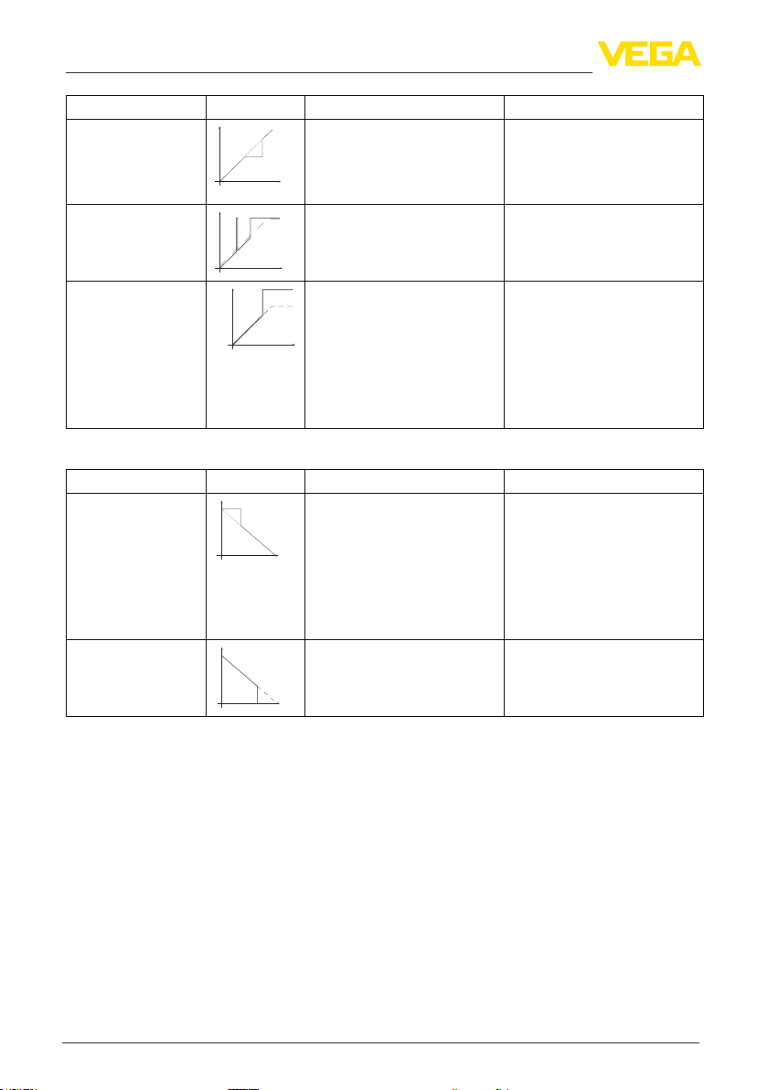
9 Diagnostics and service

time

Fault description Error pattern Cause Rectication

4. Measured value remains momentarily unchanged during ll-

Level

– Turbulence on the product

surface, quick lling

– Check parameters, change if

necessary, e.g. in dosing ves-

sel, reactor ing and then jumps to the correct level

5. Measured value jumps sporadically to

Level

– Changing condensation or

contamination on the probe

– Carry out a false signal sup-

pression

100 % during lling

6. Measured value jumps to ≥ 100 % or

0 m distance

Level

– Level echo is no longer

detected in the close range due to false signals in the close range. The sensor goes into overll protection mode. The

– Eliminate false signals in the

close range

– Check installation conditions – If possible, switch o the func-

tion "Overll protection"

max. level (0 m distance) as well as the status message "Overll protection" are outputted.

Measurement error during emptying

Fault description Error pattern Cause Rectication

7. Measured value remains unchanged in the close range during emptying

Level

– False echo larger than the level

echo

– Level echo too small

– Eliminate false signals in the

close range

– Remove contamination on the

probe. After having removed

the source of the false signals,

the false signal suppression

must be deleted.

– Carry out a new false signal

suppression

8. Measured value remains reproducible in one position during

Level

– Stored false signals in this

position are larger than the level echo

– Delete false signal memory – Carry out a new false signal

suppression

emptying

Treatment of measurement errors with bulk solids

The below tables show typical examples for application-relevant

measurement errors with bulk solids. There are two measurement

errors:

Constant level

•

Filling

•

Emptying

•

The images in column "Error pattern" show the real level with a broken line and the level displayed by the sensor as a continuous line.

44217-EN-130910

VEGAFLEX 81 • Probus PA

Level

time

9 Diagnostics and service

1 Real level 2 Level displayed by the sensor

Notes:

Wherever the sensor displays a constant value, the reason could

•

also be the fault setting of the current output to "Hold value" In case of a too low level indication, the reason could be a line

•

resistance that is too high

Measurement error with constant level

Fault description Error pattern Cause Rectication

1. Measured value shows a too low or too high level

2. Measured value jumps towards 100 %

Level

– Min./max. adjustment not

correct

– Wrong linearization curve – Adapt linearization curve

– Due to the process, the ampli-

tude of the product echo sinks

– A false signal suppression was

not carried out

– Amplitude or position of a

false echo has changed (e.g. condensation, buildup); false signal suppression no longer

matches

– Adapt min./max. adjustment

– Carry out a false signal sup-

pression

– Determine the reason for the

changed false echoes, carry

out false signal suppression,

e.g. with condensation

time

44217-EN-130910

VEGAFLEX 81 • Probus PA

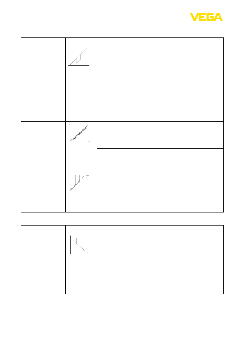
9 Diagnostics and service

time

Measurementerrorduringlling

Fault description Error pattern Cause Rectication

3. Measured value jumps towards 0 % during lling

4. Measured value uctuates around 10 … 20 %

5. Measured value jumps sporadically to 100 % during lling

Level

– Amplitude of a multiple echo

(vessel top - product surface) is larger than the level echo

– The level echo cannot be distin-

guished from the false echo at a false echo position (jumps to multiple echo)

– Transverse reection from an

extraction funnel, amplitude of the transverse reection larger than the level echo

– Various echoes from an uneven

product surface, e.g. a material

cone

– Reections from the product

surface via the vessel wall (deection)

– Varying condensation or con-

tamination on the antenna

– Check parameter "Application",

especially vessel top, type

of medium, dished end, high

dielectric constant, adapt if

necessary

– In case of interferences due to

installations in the close range:

Change polarisation direction

– Chose a more suitable installa-

tion position

– Direct sensor to the opposite

funnel wall, avoid crossing with

the lling stream

– Check parameter "Type of

medium" and adapt, if neces-

sary

– Optimize installation position

and sensor orientation

– Select a more suitable installa-

tion position, optimize sensor

orientation, e.g. with a swivel-

ling holder

– Carry out a false signal sup-

pression or increase false

signal suppression with con-

densation/contamination in the

close range by editing

– With bulk solids use radar sen-

sor with purging air connection

or exible antenna cover

Measurement error during emptying

Fault description Error pattern Cause Rectication

6. Measured value remains unchanged in

Level

the close range during emptying

– False echo larger than the level

echo

– Level echo too small

– Remove false echoes in the

close range. Check: Antenna

must protrude out of the socket

– Remove contamination on the

antenna

– In case of interferences due to

installations in the close range:

Change polarisation direction

– After removing the false ech-

oes, the false signal suppres-

sion must be deleted. Carry out

a new false signal suppression

VEGAFLEX 81 • Probus PA

44217-EN-130910

9 Diagnostics and service

time

Fault description Error pattern Cause Rectication

7. Measured value jumps sporadically towards 100 % during emptying

8. Measured value uctuates around 10 … 20 %

Level

– Varying condensation or con-

tamination on the antenna

– Various echoes from an uneven

product surface, e.g. an extraction funnel

– Reections from the product

surface via the vessel wall (deection)

– Carry out false signal suppres-

sion or increase false signal

suppression in the close range

by editing

– With bulk solids use radar sen-

sor with purging air connection

or exible antenna cover

– Check parameter "Type of

medium" and adapt, if neces-

sary

– Optimize installation position

and sensor orientation

Reaction after fault recti-

cation

24 hour service hotline

Depending on the reason for the fault and the measures taken, the steps described in chapter "Setup" must be carried out again or must be checked for plausibility and completeness.

Should these measures not be successful, please call in urgent cases the VEGA service hotline under the phone no. +49 1805 858550.

The hotline is also available outside normal working hours, seven days a week around the clock.

Since we oer this service worldwide, the support is provided in English. The service itself is free of charge, the only costs involved are the normal call charges.

9.5 Exchanging the electronics module

If the electronics module is defective, it can be replaced by the user. In Ex applications only one instrument and one electronics module

with respective Ex approval may be used. If there is no electronics module available on site, the electronics

module can be ordered through the agency serving you. The electronics modules are adapted to the respective sensor and dier in signal output or voltage supply.

The new electronics module must be loaded with the default settings of the sensor. These are the options:

In the factory

•

Or on site by the user

•

In both cases, the serial number of the sensor is needed. The serial numbers are stated on the type label of the instrument, on the inside of the housing as well as on the delivery note.

When loading on site, rst of all the order data must be downloaded from the Internet (see operating instructions manual "Electronics module").

44217-EN-130910

Exchanging the cable/rod

VEGAFLEX 81 • Probus PA

9.6 Exchanging the cable/rod

If necessary, the cable or rod (measuring part) of the probe can be exchanged.

9 Diagnostics and service

Loosen the rod or cable with a fork wrench, wrench size 7 (rod ø 8, cable ø 2 and 4) or wrench size 10 (rod ø 12).

1. Loosen the rod or cable with a fork wrench applied to the at surface, provide counterforce with another fork wrench.

2. Unscrew the loosened rod or cable manually.

3. Insert the new measuring rod carefully by hand with a twisting motion into the opening of the process tting.

4. Continue screwing in the rod manually into the opening of the process tting.

5. Exert counterforce with the second fork spanner and tighten the rod or cable on the at surfaces with the following torque.

Rod ø 8, cable ø 2 and 4: 6 Nm (4.43 lbf ft) Rod ø 12: 10 Nm (7.37 lbf ft)

Shorten cable/rod

Fig. 53: Exchange cable or rod

Information:

Please keep the stated torque so that the max. tensile strength remains.

6. Enter new probe length and if necessary the new probe type and then carry out a fresh adjustment (see "Setup procedure, Carry- ing out min. adjustment - Carrying out max. adjustment").

The rod or cable of the probe can be shortened individually.

1. Mark the requested length with mounted measuring rod.

VEGAFLEX 81 • Probus PA

44217-EN-130910

9 Diagnostics and service

2. Cable: Loosen the pins on the gravity weight (hexagon 3)

3. Cable: remove the pins

4. Cable: Pull the cable out of the gravity weight

5. Shorten the cable/rod with a cut-o wheel or metal saw at the marking. Take note of the specications in the following illustration when shortening the cable.

6. Cable with gravity weight: Shift the cable according to the drawing into the gravity weight

7. Cable with gravity weight: Fasten cable with the pins, torque 7 Nm (5.16 lbf ft)

Cable with centering weight: Fasten cable with the pins, torque 7 Nm (5.16 lbf ft) and x the clamping part on the centering weight.

8. Enter new probe length and then carry out a fresh adjustment (see "Setup procedure, Carrying out min. adjustment - Carrying out max. adjustment").

(1.77")

45 mm

(3.94")

100 mm

(0.98")

25 mm

(1.97")

50 mm

2 2 3

44217-EN-130910

VEGAFLEX 81 • Probus PA

Fig. 54: Shortening the cable probe

A Gravity weight - cable ø 4 mm B Gravity weight - cable ø 2 mm C Centering weight - cable ø 2 mm 1 Pins 2 Thread M8 for eye-bolt 3 Fixing screw - centering weight

9.7 Software update

The following components are required to update the sensor software:

Sensor

•

Voltage supply

•

Interface adapter VEGACONNECT

•

PC with PACTware

•

Current sensor software as le

•

You can nd the actual sensor software as well as detailed information of the procedure under "www.vega.com/downloads" and "Software".

9 Diagnostics and service

You can nd information about the installation in the download le.

Caution:

Instruments with approvals can be bound to certain software versions. Therefore make sure that the approval remains eective with a software update.

You can nd detailed information on www.vega.com/downloads and "Approvals".

9.8 How to proceed in case of repair

You can nd a repair form as well as detailed information on how to

proceed under www.vega.com/downloads and "Formsandcerti- cates".

By doing this you help us carry out the repair quickly and without having to call back for needed information.

If a repair is necessary, please proceed as follows:

Print and ll out one form per instrument

•

Clean the instrument and pack it damage-proof

•

Attach the completed form and, if need be, also a safety data

•

sheet outside on the packaging Please contact for the return shipment the agency serving you. You

•

can nd the agency on our home page www.vega.com.

44217-EN-130910

VEGAFLEX 81 • Probus PA

10 Dismounting

10.1 Dismounting steps

Warning:

Before dismounting, be aware of dangerous process conditions such as e.g. pressure in the vessel or pipeline, high temperatures, corrosive or toxic products etc.

Take note of chapters "Mounting" and "Connecting to power supply" and carry out the listed steps in reverse order.

10.2 Disposal

The instrument consists of materials which can be recycled by specialised recycling companies. We use recyclable materials and have designed the parts to be easily separable.

Correct disposal avoids negative eects on humans and the environment and ensures recycling of useful raw materials.

Materials: see chapter "Technical data" If you have no way to dispose of the old instrument properly, please

WEEE directive 2002/96/EG

This instrument is not subject to the WEEE directive 2002/96/EG and the respective national laws. Pass the instrument directly on to a specialised recycling company and do not use the municipal collecting points. These may be used only for privately used products according to the WEEE directive.

44217-EN-130910

VEGAFLEX 81 • Probus PA

11 Supplement

11.1 Technical data

General data

316L corresponds to 1.4404 or 1.4435 Materials, wetted parts

Ʋ Process tting (version up to 6 bar) 316L and PPS GF 40 Ʋ Process tting (version up to 40 bar) 316L and Aluminium oxide-ceramic 99.7 % (Al2O3),

Ʋ Process seal on the instrument side

(cable/rod leadthrough)

Ʋ Process seal On site (instruments with thread: Klingersil C-4400 is

Ʋ Rod: ø 8 mm (0.315 in) 316L or Hastelloy C22 (2.4602) Ʋ Rod: ø 12 mm (0.472 in) 316L or Hastelloy C22 (2.4602) Ʋ Cable: ø 2 mm (0.079 in) 316 (1.4401) Ʋ Cable: ø 4 mm (0.157 in) 316 (1.4401) Ʋ Inner conductor (up to the cable) 316L Ʋ Gravity weight (optionally available) 316L Ʋ Centering weight (optionally available) 316L

Materials, non-wetted parts

Ʋ Plastic housing plastic PBT (Polyester) Ʋ Aluminium die-casting housing Aluminium die-casting AlSi10Mg, powder-coated - basis:

Ʋ Stainless steel housing - precision

casting

Ʋ Stainless steel housing, electropol-

ished

Ʋ Second line of defence (optional) Borosilicate glass GPC 540 Ʋ Seal between housing and housing

cover

Ʋ Inspection window in housing cover

(optional)

Ʋ Ground terminal 316L

Ohmic contact Between ground terminal, process tting and probe

Process ttings

Ʋ Pipe thread, cylindrical (ISO 228 T1) G¾, G1, G1½ according to DIN 3852-A Ʋ American pipe thread, conical

(ASME B1.20.1)

Ʋ Flanges e.g. DIN from DN 25, ANSI from 1"

Hastelloy C22 (2.4602) and Aluminium oxide-ceramic

99.7 % (Al2O3) FKM (SHS FPM 70C3 GLT), FFKM (Kalrez 6375),

EPDM (A+P 75.5/KW75F), silicone FEP coated (A+P FEP-O-SEAL)

attached)

Polyester 316L

316L

NBR (stainless steel housing, precision casting), silicone (aluminium/plastic housing; stainless steel housing, electropolished)

Polycarbonate (with Ex d version: glass)

¾ NPT, 1 NPT, 1½ NPT

44217-EN-130910

VEGAFLEX 81 • Probus PA

Weight

Ʋ Instrument weight (depending on

approx. 0.8 … 8 kg (0.176 … 17.64 lbs)

process tting)

Ʋ Rod: ø 8 mm (0.315 in) approx. 400 g/m (4.3 oz/ft) Ʋ Rod: ø 12 mm (0.472 in) approx. 900 g/m (9.68 oz/ft) Ʋ Cable: ø 2 mm (0.079 in) approx. 16 g/m (0.17 oz/ft) Ʋ Cable: ø 4 mm (0.157 in) approx. 60 g/m (0.65 oz/ft) Ʋ Gravity weight for cable ø 2 mm

100 g (3.22 oz)

(0.079 in)

Ʋ Gravity weight for cable ø 4 mm

200 g (6.43 oz)

(0.157 in)

Ʋ Centering weight ø 40 mm (1.575 in) 180 g (5.79 oz) Ʋ Centering weight ø 45 mm (1.772 in) 250 g (8.04 oz) Ʋ Centering weight ø 75 mm (2.953 in) 825 g (26.52 oz) Ʋ Centering weight (ø 95 mm (3.74 in) 1050 g (33.76 oz)

Probe length L (from seal surface)

Ʋ Rod: ø 8 mm (0.315 in) up to 6 m (19.69 ft) Ʋ Rod: ø 12 mm (0.472 in) up to 6 m (19.69 ft) Ʋ Trimming accuracy - rod ±1 mm Ʋ Cable: ø 2 mm (0.079 in) up to 75 m (246.1 ft) Ʋ Cable: ø 4 mm (0.157 in) up to 75 m (246 ft) Ʋ Trimming accuracy - cable ±0.05 %

Lateral load

Ʋ Rod: ø 8 mm (0.315 in) 10 Nm (7.38 lbf ft) Ʋ Rod: ø 12 mm (0.472 in) 30 Nm (22.13 lbf ft)

Max. tensile load

Ʋ Cable: ø 2 mm (0.079 in) 1.5 KN (337 lbf) Ʋ Cable: ø 4 mm (0.157 in) 2.5 KN (562 lbf)

Thread in gravity weight, e.g. for eye-bolt

M 8

(cable version) Torque for exchangeable cable or rod probe (in the process tting)

Ʋ Cable: ø 2 mm (0.079 in) 6 Nm (4.43 lbf ft) Ʋ Cable: ø 4 mm (0.157 in) 6 Nm (4.43 lbf ft) Ʋ Rod: ø 8 mm (0.315 in) 6 Nm (4.43 lbf ft) Ʋ Rod: ø 12 mm (0.472 in) 10 Nm (7.38 lbf ft)

Torque for NPT cable glands and Conduit tubes

Ʋ Plastic housing max. 10 Nm (7.376 lbf ft) Ʋ Aluminium/Stainless steel housing max. 50 Nm (36.88 lbf ft)

11 Supplement

Input variable

Measured variable Level of liquids Min. dielectric constant of the medium

44217-EN-130910

VEGAFLEX 81 • Probus PA

11 Supplement

Ʋ Cable probes εr ≥ 1.6 Ʋ Rod probes εr ≥ 1.6

1 1

Fig. 55: Measuring ranges - VEGAFLEX 81

1 Reference plane 2 Probe length L 3 Measuring range (default setting refers to the measuring range in water) 4 Upper dead band (see diagrams under Accuracy - grey section) 5 Lower dead band (see diagrams under Accuracy - grey section)

Output variable

Output signal digital output signal, format according to IEEE-754 Sensor address 126 (default setting) Damping (63 % of the input variable) 0 … 999 s, adjustable Probus PA prole 3.02

44217-EN-130910

VEGAFLEX 81 • Probus PA

11 Supplement

Number of FBs with AI (function blocks

with analogue input) Default values

Ʋ 1. FB PV Ʋ 2. FB SV 1 Ʋ 3. FB SV 2

Current value

Ʋ Non-Ex and Ex ia instrument 10 mA, ±0.5 mA Ʋ Ex-d instruments 16 mA, ±0.5 mA

Resolution, digital < 1 mm (0.039 in)

Accuracy (according to DIN EN 60770-1)

Process reference conditions according to DIN EN 61298-1

Ʋ Temperature +18 … +30 °C (+64 … +86 °F) Ʋ Relative humidity 45 … 75 % Ʋ Air pressure +860 … +1060 mbar/+86 … +106 kPa

(+12.5 … +15.4 psig)

Installation reference conditions

Ʋ Min. distance to installations > 500 mm (19.69 in) Ʋ Vessel metallic, ø 1 m (3.281 ft), centric installation, process

tting ush with the vessel ceiling

Ʋ Medium Water/Oil (dielectric constant ~2.0)

Ʋ Installation Probe end does not touch the vessel bottom Sensor parameter adjustment No gating out of false signals carried out Typical deviation - Interface measure-

± 5 mm (0.197 in)

ment

Typical deviation - Total level interface

See following diagrams

measurement

Typical deviation - Level measurement

2)3)

See following diagrams

With interface measurement = 2.0

Depending on the installation conditions, there can be deviations which can be rectied with an adaptation of

the adjustment or a change of the measured value oset in the DTM service mode

The dead bands can be optimizes by a false signal suppression.

44217-EN-130910

VEGAFLEX 81 • Probus PA

11 Supplement

15mm

(0.591

2mm

(0.079

-2mm

(-0.079

-10mm

(-0.394

0,08 m (3.15")

0,3 m

(11.811

Fig. 56: Deviation VEGAFLEX 81 in rod version in water

1 Dead band - no measurement possible in this area L Probe length

15mm

(0.591

2mm

(0.079

-2mm

(-0.079

-10mm

(-0.591

0,15 m

(5.906

0,3 m

(11.811

0,02 m

(0.787

0,07 m

(2.756

0,05 m (1.97

Fig. 57: Deviation VEGAFLEX 81 in rod version in oil

1 Dead band - no measurement possible in this area L Probe length

44217-EN-130910

VEGAFLEX 81 • Probus PA

15mm

(0.591

2mm

(0.079

-2mm

(-0.079

10mm

(0.394

0,08 m (3.15

0,3 m

(11.811

Fig. 58: Deviation VEGAFLEX 81 in cable version in water

1 Dead band - no measurement possible in this area L Probe length

15mm

(0.591

2mm

(0.079

-2mm

(-0.079

11 Supplement

0,1 m

(3.94

-15mm

(-0.591

0,15 m

0,3 m

(5.906

(11.811

Fig. 59: Deviation VEGAFLEX 81 in cable version ø 2 mm (0.079 in), in oil

1 Dead band - no measurement possible in this area L Probe length

44217-EN-130910

VEGAFLEX 81 • Probus PA

1 1

0,05 m

(1.969

0,08 m (3.15

11 Supplement

20mm

(0.787

15mm

(0.591

2mm

(0.079

-2mm

(-0.079

-15mm )

(-0.591

0,3 m

0,15 m

(5.906

(11.811

0,05 m

(1.969

0,15 m

(5.906

Fig. 60: Deviation VEGAFLEX 81 in cable version ø 4 mm (0.157 in), in oil

1 Dead band - no measurement possible in this area L Probe length

Repeatability ≤ ±1 mm

Variablesinuencingmeasurementaccuracy

Temperature drift - Digital output ±3 mm/10 K relating to the max. measuring range or

max. 10 mm (0.394 in)

1 1

Additional deviation through electromag-

< ±10 mm (< ±0.394 in)

netic interference acc. to EN 61326

Inuenceofthesuperimposedgasandpressuretotheaccuracy

The propagation speed of the radar impulses in gas or vapour above the medium is reduced by high pressure. This eect depends on the superimposed gas or vapour and is especially large at low temperatures.

The following table shows the resulting deviation for some typical gases and vapours. The specied values refer to the distance. Positive values mean that the measured distance is too large, negative values that the measured distance is too small.

Gas phase Temperature Pressure

1 bar (14.5 psig) 10 bar (145 psig) 50 bar (725 psig)

Air 20 °C/68 °F 0.00 % 0.22 % 1.2 %

200 °C/392 °F -0.01 % 0.13 % 0.74 %

400 °C/752 °F -0.02 % 0.08 % 0.52 %

Hydrogen 20 °C/68 °F -0.01 % 0.10 % 0.61 %

200 °C/392 °F -0.02 % 0.05 % 0.37 %

400 °C/752 °F -0.02 % 0.03 % 0.25 %

44217-EN-130910

VEGAFLEX 81 • Probus PA

11 Supplement

Gas phase Temperature Pressure

1 bar (14.5 psig) 10 bar (145 psig) 50 bar (725 psig)

Steam (saturated steam)

100 °C/212 °F 0.26 % - -

180 °C/356 °F 0.17 % 2.1 % -

264 °C/507 °F 0.12 % 1.44 % 9.2 %

366 °C/691 °F 0.07 % 1.01 % 5.7 %

Characteristics and performance data

Measuring cycle time < 500 ms Step response time

≤ 3 s

Max. lling/emptying speed 1 m/min

Ambient conditions

Ambient, storage and transport tempera-

-40 … +80 °C (-40 … +176 °F)

ture

Process conditions

For the process conditions, please also note the specications on the type label. The lowest value always applies.

The measurement error from the process conditions is in the specied pressure and temperature range of below 1 %.

Process pressure

Ʋ Process tting with PPS GF 40 -1 … 6 bar/-100 … 600 kPa (-14.5 … 87 psi), depending

on the process tting

Ʋ Process tting with Al2O

Vessel pressure relating to the ange nominal stage

-1 … +40 bar/-100 … +4000 kPa (-14.5 … +580 psig), depending on the process tting

see supplementary instructions manual "Flanges ac- cording to DIN-EN-ASME-JIS"

Process temperature (thread or ange temperature)

Ʋ PPS GF 40 -40 … +80 °C (-40 … +176 °F) Ʋ FKM (SHS FPM 70C3 GLT) -40 … +150 °C (-40 … +302 °F) Ʋ EPDM (A+P 75.5/KW75F) -40 … +150 °C (-40 … +302 °F) Ʋ Silicone FEP coated (A+P FEP-O-

-40 … +150 °C (-40 … +302 °F)

SEAL)

Ʋ FFKM (Kalrez 6375) -20 … +150 °C (-4 … +302 °F) Ʋ FFKM (Kalrez 6375) - with tempera-

-20 … +200 °C (-4 … +392 °F)

ture adapter

Time span after a sudden measuring distance change by max. 0.5 m in liquid applications, max 2 m with bulk

solids applications, until the output signal has taken for the rst time 90 % of the nal value (IEC 61298-2).

44217-EN-130910

VEGAFLEX 81 • Probus PA

11 Supplement

80°C

(176°F)

65°C

(149°F)

3 4

-40°C

(-104°F)

0°C

(32°F)

-40°C

(-104°F)

80°C

(176°F)

130°C

(266°F)

150°C

(302°F)

Fig. 61: Ambient temperature - process temperature, standard version

1 Ambient temperature 2 Process temperature (depending on the seal material) 3 Maximum permissible temperature - standard 4 Limited temperature range - plastic housing and stainless steel housing, electropolished

80°C

(176°F)

3 4

55°C

(131°F)

-20°C

(-68°F)

0°C

(32°F)

-40°C

(-104°F)

150°C

(302°F)

200°C

(392°F)

Fig. 62: Ambient temperature - process temperature, version with temperature adapter

Vibration resistance

Ʋ Instrument housing 4 g at 5 … 200 Hz according to EN 60068-2-6 (vibration

with resonance)

Ʋ Rod probe 1 g with 5 … 200 Hz according EN 60068-2-6 (vibration

at resonance) with rod length 50 cm (19.69 in)

Shock resistance

Ʋ Instrument housing 100 g, 6 ms according to EN 60068-2-27 (mechanical

shock)

Ʋ Rod probe 25 g, 6 ms according to EN 60068-2-27 (mechanical

shock) with rod length 50 cm (19.69 in)

44217-EN-130910

VEGAFLEX 81 • Probus PA

11 Supplement

Electromechanical data - version IP 66/IP 67 and IP 66/IP 68; 0.2 bar

Options of the cable entry

Ʋ Cable gland M20 x 1.5 (cable: ø 5 … 9 mm) Ʋ Cable entry ½ NPT Ʋ Blind plug M20 x 1.5; ½ NPT Ʋ Closing cap M20 x 1.5; ½ NPT

Plug options

Ʋ Signal circuit Plug M12 x 1, according to ISO 4400, Harting HAN,

7/8" FF

Ʋ Indication circuit M12 x 1 plug

Wire cross-section (spring-loaded terminals)

Ʋ Massive wire, cord 0.2 … 2.5 mm² (AWG 24 … 14) Ʋ Stranded wire with end sleeve 0.2 … 1.5 mm² (AWG 24 … 16)

Electromechanical data - version IP 66/IP 68 (1 bar)

Options of the cable entry

Ʋ Cable gland with integrated connec-

M20 x 1.5 (cable: ø 5 … 9 mm)

tion cable

Ʋ Cable entry ½ NPT Ʋ Blind plug M20 x 1.5; ½ NPT

Connection cable

Ʋ Wire cross-section 0.5 mm² (AWG 20) Ʋ Wire resistance < 0.036 Ω/m Ʋ Tensile strength < 1200 N (270 lbf) Ʋ Standard length 5 m (16.4 ft) Ʋ Max. length 180 m (590.6 ft) Ʋ Min. bending radius 25 mm (0.984 in) with 25 °C (77 °F) Ʋ Diameter approx. 8 mm (0.315 in) Ʋ Colour - Non-Ex version Black Ʋ Colour - Ex-version Blue

Display and adjustment module

Display element Display with backlight Measured value indication

Ʋ Number of digits 5 Ʋ Size of digits W x H = 7 x 13 mm

Adjustment elements 4 keys Protection rating

Ʋ unassembled IP 20 Ʋ mounted into the housing without

IP 40

cover

Materials

Ʋ Housing ABS

44217-EN-130910

VEGAFLEX 81 • Probus PA

11 Supplement

Ʋ Inspection window Polyester foil

Integrated clock

Date format Day.Month.Year Time format 12 h/24 h Time zone Ex factory CET Rate deviation max. 10.5 min/year

Measurement electronics temerature

Resolution 1 °C (1.8 °F) Accuracy ±1 °C (1.8 °F)

Voltage supply

Operating voltage

Ʋ Non-Ex instrument 9 … 32 V DC Ʋ EEx-ia instrument - Power supply

9 … 17.5 V DC

FISCO model

Ʋ EEx-ia instrument - Power supply

9 … 24 V DC

ENTITY model

Ʋ EEx-d instrument 14 … 32 V DC

Number of sensors per DP/PA segment coupler, max.

Ʋ Non-Ex 32 Ʋ Ex 10

Electrical protective measures

Protection, depending on housing version

Ʋ Plastic housing IP 66/IP 67 Ʋ Aluminium housing, stainless steel

IP 66/IP 68 (0.2 bar) housing - investment casting, stainless steel housing - electro-polished

Ʋ Aluminium and stainless housing, in-

IP 66/IP 68 (1 bar) vestment casting (optionally available)

Overvoltage category III Protection class III

Approvals

Instruments with approvals can have dierent technical data depending on the version. For that reason the associated approval documents of these instruments must be carefully noted.

They are part of the delivery or can be downloaded under www.vega.com and "VEGA Tools" as well as under "Downloads" and "Approvals".

11.2 CommunicationProbusPA

Instrumentmasterle

The instrument master le (GSD) contains the characteristic data of the Probus PA instrument.

The prerequisites for maintaining the protection rating are a suitable cable as well as correct mounting.

VEGAFLEX 81 • Probus PA

44217-EN-130910

11 Supplement

These data are, e.g. the permissible transmission rates as well as information on diagnostics values and the format of the measured value outputted by the PA instrument.

A bitmap le is also provided for the Probus network planning tool. This le is installed automatically when the GSD le is integrated. The bitmap le is used for symbolic indication of the PA instrument in the conguration tool.

ID number

Each Probus instrument gets an unambiguous ident number (ID number) from the Probus user organisation (PNO). This ID number is also included in the name of the GSD le. Optionally to this manufacturer-specic GSD le, PNO provides also a general so-called prole-specic GSD le. If the general GSD le is used, the sensor must be set to the prole-specic ident number via the DTM software. By default, the sensor operates with the manufacturer-specic ID number. When using the instruments on a segment coupler SK-2 or SK-3, no special GSD les are required.

VE010BF5 The following table shows the instrument ID and the GSD names for the VEGAFLEX sensor series.

Device name Instrument ID GSDlename

VEGA Instrument class in

prole3.02

VEGAFLEX Serie 80 0xBF5 0x9702 VE010BF5.GSD PA139702.GSD

VEGA Prole-specic

Cyclicaldatatrac

The master class 1 (e.g. PLC) cyclically reads out measured values from the sensor during operation. The below block diagram below shows which data can be accessed by the PLC.

44217-EN-130910

VEGAFLEX 81 • Probus PA

11 Supplement

Fig. 63: VEGAFLEX 81: Block diagram with AI FB 1 … AI FB 3 OUT values

TB Transducer Block FB 1 … FB 3 Function Block

Module of the PA sensors

For the cyclic data trac, VEGAFLEX 81 provides the following modules:

AI FB1 (OUT)

•

– Out value of the AI FB1 after scaling

AI FB2 (OUT)

•

– Out value of the AI FB2 after scaling

AI FB3 (OUT)

•

– Out value of the AI FB3 after scaling

Free Place

•

– This module must be used if a value in the data telegram of the cyclical data trac should not

be used (e.g. replacement of temperature and Additional Cyclic Value)

A maximum of three modules can be active. By means of the conguration software of the Probus master you can determine the conguration of the cyclical data telegram with these modules. The procedure depends on the respective conguration software.

Note:

The modules are available in two versions:

Short for Probus master supporting only one "Identier Format" byte, e.g. Allen

•

Bradley

VEGAFLEX 81 • Probus PA

44217-EN-130910

11 Supplement

Sign

-23

Long for Probus master only supporting the "Identier Format" byte, e.g. Siemens

•

S7-300/400

Examplesoftelegramconguration

In the following you will see how the modules can be combined and how the appendant data telegram is structured.

Example 1

AI FB1 (OUT)

•

AI FB2 (OUT)

•

AI FB3 (OUT)

•

ByteNo.

Format IEEE-754-Floating point

Value AI FB1 (OUT) AI FB1 AI FB2 (OUT) AI FB2 AI FB3 (OUT) AI FB3

Example 2

•

Byte-No. 1 2 3 4 5

Format IEEE-754-Floating point value Status

Value AI FB1 (OUT) AI FB1

1 2 3 4 5 6 7 8 9 10 11 12 13 14 15

value

Status IEEE-754-Floating point

value

Status IEEE-754-Floating point

value

AI FB1 (OUT) Free Place Free Place

Note:

Bytes 6-15 are not used in this example.

Status

44217-EN-130910

Data format of the output signal

Byte0

Byte4

Byte3

Status Value (IEEE-754)

Fig. 64: Data format of the output signal

The status byte corresponds to prole 3.02 "Probus PA Prole for Process Control Devices" coded. The status "Measured value OK" is coded as 80 (hex) (Bit7 = 1, Bit6 … 0 = 0).

The measured value is transferred as a 32 bit oating point number in the IEEE-754 format.

Byte n

Bit

6543

Exponent

Bit

Value = (-1)

Fig. 65: Data format of the measured value

VEGAFLEX 81 • Probus PA

Byte1

Byte2

Bit

210-1

(Exponent - 127)

Byte n+1

Bit

7 2

Bit

-2-3-4-5-6 -7

Significant

(1 + Significant)

Bit

Byte n+2

Bit

3 2

Bit

-9

Bit

-10 -11

Bit

-8

Bit

-12

-13

-14 -15

Significant

Byte n+3 Bit

Bit

-16

Bit

-17

Bit

-19

-18

Bit

-20

-22

-21

Significant

11 Supplement

Coding of the status byte associated with the PA output value

You can nd further information for the coding of the status byte in the Device Description 3.02 on www.probus.com.

Status code Description according to

Probusstandard

0 x 00 bad - non-specic Flash-Update active

0 x 04 bad - conguration error – Adjustment error

0 x 0C bad - sensor failure – Hardware error

0 x 10 bad - sensor failure – Measured value generation error

0 x 1f bad - out of service con-

stant

0 x 44 uncertain - last unstable

value

0 x 48 uncertain substitute set – Switch on simulation

0 x 4c uncertain - initial value Failsafe replacement value (Failsafe-Mode = "Last valid

0 x 51 uncertain - sensor; con-

version not accurate - low limited

0 x 52 uncertain - sensor; con-

version not accurate - high limited

0 x 80 good (non-cascade) - OK OK

0 x 84 good (non-cascade) - ac-

tive block alarm

0 x 89 good (non-cascade) - ac-

tive advisory alarm - low limited

0 x 8a good (non-cascade) - ac-

tive advisory alarm - high limited

0 x 8d good (non-cascade) - ac-

tive critical alarm - low limited

0 x 8e good (non-cascade) - ac-

tive critical alarm - high limited

Possible cause

– Conguration error with PV-Scale (PV-Span too

small)

– Unit irregularity – Error in the linearization table

– Converter error – Leakage pulse error – Trigger error

– Temperature measurement error

"Out of Service" mode switched on

Failsafe replacement value (Failsafe-Mode = "Last value" and already valid measured value since switching on)

– Failsafe replacement value (Failsafe-Mode = "Fsafe

value")

value" and no valid measured value since switching on)

Sensor value < lower limit

Sensor value > upper limit

Static revision (FB, TB) changed (10 sec. active, after the parameter of the static category has been written)

Lo-Alarm

Hi-Alarm

Lo-Lo-Alarm

Hi-Hi-Alarm

44217-EN-130910

VEGAFLEX 81 • Probus PA

11 Supplement

11.3 Dimensions

The following dimensional drawings represent only an extract of all possible versions. Detailed dimensional drawings can be downloaded at www.vega.com/downloads under "Drawings".

Plastic housing

~ 69 mm

(2.72")

ø 79 mm

(3.11")

~ 84 mm

(3.31")

M16x1,5

ø 79 mm

(3.11")

M20x1,5/ ½ NPT

(4.41")

112 mm

M20x1,5/ ½ NPT

(4.41")

112 mm

Fig. 66: Housing versions in protection IP 66/IP 68 (0.2 bar) - with integrated display and adjustment module the housing is 9 mm/0.35 in higher

1 Single chamber version 2 Double chamber version

Aluminium housing

~ 116 mm

(4.57")

ø 86 mm

(3.39")

(4.57")

116 mm

M20x1,5/ ½ NPT

M20x1,5

Fig. 67: Housing versions in protection IP 66/IP 68 (0.2 bar) - with integrated display and adjustment module the housing is 9 mm/0.35 in higher

1 Single chamber version 2 Double chamber version

~ 87 mm

M16x1,5

M20x1,5/ ½ NPT

(3.43")

ø 86 mm

(3.39")

(4.72")

120 mm

44217-EN-130910

VEGAFLEX 81 • Probus PA

11 Supplement

Aluminium housing in protection rating IP 66/IP 68 (1 bar)

~ 150 mm

(5.91")

ø 86 mm

(3.39")

(4.57")

116 mm

M20x1,5

Fig.68:HousingversionsinprotectionIP␣66/IP␣68(1␣bar)-withintegrateddisplayandadjustmentmodulethe housingis9␣mm/0.35␣inhigher

1 Single chamber version 2 Double chamber version

~ 105 mm

(4.13")

M20x1,5/ ½ NPT

ø 86 mm

(3.39")

M16x1,5

(4.72")

120 mm

Stainless steel housing

~ 59 mm

(2.32")

ø 80 mm

(3.15")

~ 69 mm

(2.72")

ø 79 mm

(3.11")

~ 87 mm

M16x1,5

(3.43")

ø 86 mm

(3.39")

M20x1,5/ ½ NPT

(4.41")

112 mm

M20x1,5/ ½ NPT

(4.61")

117 mm

M20x1,5/ ½ NPT

321

(4.72")

120 mm

Fig. 69: Housing versions in protection IP 66/IP 68 (0.2 bar) - with integrated display and adjustment module the housing is 9 mm/0.35 in higher

1 Single chamber version, electropolished 2 Single chamber version, precision casting 3 Double chamber version, precision casting

VEGAFLEX 81 • Probus PA

44217-EN-130910

Stainless steel housing in protection rating IP 66/IP 68, 1 bar

~ 93 mm

(3.66")

ø 80 mm

(3.15")

~ 103 mm

(4.06")

ø 79 mm

(3.11")

~ 105 mm

(4.13")

11 Supplement

ø 86 mm

(3.39")

M16x1,5

(4.61")

117 mm

M20x1,5/ ½ NPT

120 mm

M20x1,5/ ½ NPT

(4.41")

112 mm

M20x1,5

Fig.70:HousingversionsinprotectionIP␣66/IP␣68(1␣bar)-withintegrateddisplayandadjustmentmodulethe housingis9␣mm/0.35␣inhigher

1 Single chamber version, electropolished 2 Single chamber version, precision casting 3 Double chamber version, precision casting

(4.72")

44217-EN-130910

VEGAFLEX 81 • Probus PA

11 Supplement

VEGAFLEX 81, cable version with gravity weight

SW 36 (1. SW 41 (1. SW 46 (1.

ø 2 mm (0.08")

42")

(G¾, ¾ NPT)

61")

(G1, 1 NPT)

81")

(G1½, 1½ NPT)

G¾, ¾ NPT, G1, 1 NPT, G1½, 1½ NPT

ø 16 mm

(0.63")

ø 20 mm

(0.79")

(1.97")

50 mm

ø 4 mm

(0.16")

ø 16 mm

(0.63")

ø 20 mm

(0.79")

46 mm

(1.81")

(0.87")

22 mm

100 mm (3.94")

ø 4 mm

(0.16")

1 2 3

ø 16 mm

(0.63")

ø 20 mm

(0.79")

(3.78")

96 mm

(0.87")

22 mm

100 mm (3.94")

44217-EN-130910

Fig. 71: VEGAFLEX 81, threaded version with gravity weight (all gravity weights with thread M8 for eye-bolt)

L Sensor length, see chapter "Technical data"

VEGAFLEX 81 • Probus PA

1 Cable version ø 2 mm (0.079 in) with gravity weight 2 Cable version ø 4 mm (0.157 in) with gravity weight 3 Cable version with temperature adapter

VEGAFLEX 81, cable version with centering weight

SW 36 (1.

42")

(G¾, ¾ NPT)

61")

SW 41 (1. SW 46 (1.

(G1, 1 NPT)

(G1½, 1½ NPT)

81")

G¾, ¾ NPT, G1, 1 NPT, G1½, 1½ NPT

11 Supplement

(1.81")

22 mm (0.87") 46 mm

(1.18")

30 mm

ø 2 mm

(0.08")

ø 4 mm (0.16")

(1.18")

30 mm

1 2

Fig. 72: VEGAFLEX 81, threaded version

L Sensor length, see chapter "Technical data" x ø 40 mm (1.57 in)

ø 45 mm (1.77 in) ø 75 mm (2.95 in)

ø 95 mm (3.74 in) 1 Cable version ø 2 mm (0.079 in) with centering weight (see supplementary instructions "Centering") 2 Cable version ø 4 mm (0.157 in) with centering weight (see supplementary instructions "Centering")

44217-EN-130910

VEGAFLEX 81 • Probus PA

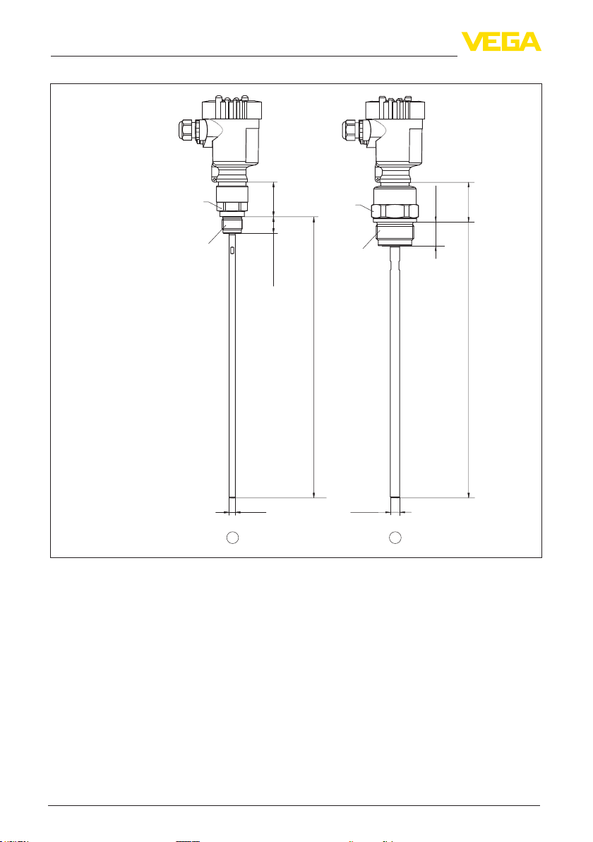
11 Supplement

VEGAFLEX 81, rod version

SW 36 (1.

42")

(G¾, ¾ NPT)

61")

SW 41 (1. SW 46 (1.

(G1, 1 NPT)

(G1½, 1½ NPT)

81")

G¾, ¾ NPT, G1, 1 NPT, G1½, 1½ NPT

ø 8 mm

(0.32")

1 2

Fig. 73: VEGAFLEX 81, threaded version

L Sensor length, see chapter "Technical data" 1 Rod version ø 8 mm (0.315 in) 2 Rod version ø 12 mm (0.472 in)

46 mm

(1.81")

22 mm (0.87")

SW 55

(2.17")

G1½, 1½ NPT

ø 12¨mm

(0.47")

(1.18")

30mm

51 mm

(2.01")

100

44217-EN-130910

VEGAFLEX 81 • Probus PA

VEGA FLEX81 User Manual

Specifications and Main Features

Frequently Asked Questions

User Manual

Quick start

1 About this document

1.1 Function

1.2 Target group

1.3 Symbolism used

2 For your safety

2.1 Authorised personnel

2.2 Appropriate use

2.3 Warning about incorrect use

2.4 General safety instructions

2.5 CE conformity

2.6 NAMUR recommendations

2.7 Environmental instructions

3 Product description

3.2 Principle of operation

3.3 Packaging, transport and storage

3.4 Accessories and replacement parts

4 Mounting

4.1 General instructions

4.2 Mounting instructions

5 Connecting to power supply

5.1 Preparing the connection

5.2 Connecting

5.3 Wiring plan, single chamber housing

5.4 Wiring plan, double chamber housing

5.5 Wiring plan, Ex-d-ia double chamber housing

5.6 Wiring plan - version IP 66/IP 68, 1 bar

5.7 Supplementary electronics

5.8 Set instrument address

5.9 Switch-on phase

6 Set up with the display and adjustment module

6.1 Insert display and adjustment module

6.2 Adjustment system

6.3 Parameter adjustment - Quick setup

6.4 Parameter adjustment - Extended adjustment

6.5 Saving the parameter adjustment data

7 Setup with PACTware

7.1 Connect the PC

7.2 Parameter adjustment with PACTware

7.3 Set up with the quick setup

7.4 Saving the parameter adjustment data

8 Set up with other systems

8.1 DD adjustment programs

9 Diagnostics and service

9.1 Maintenance

9.2 Diagnosis memory

9.3 Status messages

9.4 Rectify faults

9.5 Exchanging the electronics module

9.6 Exchanging the cable/rod

9.7 Software update

9.8 How to proceed in case of repair

10 Dismounting

10.1 Dismounting steps

10.2 Disposal

11 Supplement

11.1 Technical data

11.3 Dimensions