

Page 1
Perspective-SS
-- Sidescan Processing Guide --
Software Version 7.6
By:
Tony M. Ramirez
September, 2014
Page 2

Triton Imaging Inc.
Engineering Office
2121 41st Avenue, Suite 211
Capitola, CA 95010
USA
831-722-7373
831-475-8446
sales@tritonimaginginc.com
support@tritonimaginginc.com
© 2014 TRITON
This user guide is provided as a means to become familiar with TRITON’s software through an explanation of the
options available for processing sidescan data. The user interface presented in this guide is subject to change to
accommodate software upgrades and revisions. While every precaution has been taken to eliminate errors in this
guide, TRITON assumes no responsibility for errors in this document.
Users of this document are required to have a valid license for Perspective and MosaicOne in order to activate the
software. TRITON hereby grants licensees of TRITON’s software the right to reproduce this document for
internal use only.
Page ii
Page 3

Table of Contents
1.0 Introduction ................................................................................................. 1
2.0 Settings ...................................................................................................... 1
2.1 File Paths .............................................................................................................................................................................. 1
2.2 Number of Cores .................................................................................................................................................................. 1
3.0 Import ....................................................................................................... 2
3.1 File Import ............................................................................................................................................................................ 2
3.2 Projection/Datum ................................................................................................................................................................ 2
3.3 Navigation ............................................................................................................................................................................ 3
3.4 Import Processing Option .................................................................................................................................................... 4
4.0 Review ........................................................................................................ 4
4.1 Launch Waterfall Display ..................................................................................................................................................... 4
4.2 Bottom Tracking ................................................................................................................................................................... 6
4.3 TVG Adjustments ................................................................................................................................................................. 8
5.0 Process ...................................................................................................... 11
5.1 Sidescan Mosaic Wizard..................................................................................................................................................... 11
5.1.1 Choose/Create Mosaic File ......................................................................................................................................... 11
5.1.2 Choose Mosaic Settings .............................................................................................................................................. 12
5.1.3 Select/Order Input Lines ............................................................................................................................................. 13
5.1.4 Geometry Settings ...................................................................................................................................................... 13
5.1.5 Line and Channel Settings .......................................................................................................................................... 14
5.1.6 Corrections and Filters................................................................................................................................................ 16
5.2 Re-merge Mosaic ............................................................................................................................................................... 18
5.3 Other Processing Options .................................................................................................................................................. 19
5.3.1 Navigation Processing ................................................................................................................................................ 19
5.3.2 Merge Lines ................................................................................................................................................................ 19
5.3.3 Move Line ................................................................................................................................................................... 19
5.3.4 Add Lines .................................................................................................................................................................... 19
5.3.5 Remove Lines .............................................................................................................................................................. 19
5.3.6 Single Channel Auto Flip ............................................................................................................................................. 19
6.0 Enhance ..................................................................................................... 20
6.1 Color Settings ..................................................................................................................................................................... 20
6.2 Histogram........................................................................................................................................................................... 20
7.0 Interpret ................................................................................................... 22
7.1 dB-based Imagery .............................................................................................................................................................. 22
7.2 Interactive Waterfall Display ............................................................................................................................................. 22
7.3 TargetOne .......................................................................................................................................................................... 23
7.4 SeaClass ............................................................................................................................................................................. 23
8.0 Export ....................................................................................................... 24
8.1 GeoTiff ............................................................................................................................................................................... 24
8.2 KML .................................................................................................................................................................................... 24
9.0 Workflow ................................................................................................... 25
Page iii
Page 4
1.0 Introduction
This document presents a sample workflow for processing sidescan data using Triton’s
Perspective software. Also covered are some of the interpretation tools available in
Perspective and a brief discussion of export options. Having Perspective open and
following the steps outlined in this document from start to end will provide the user with a
basic understanding of how the software works and the tools available with the MosaicOne
sidescan processing module in Perspective.
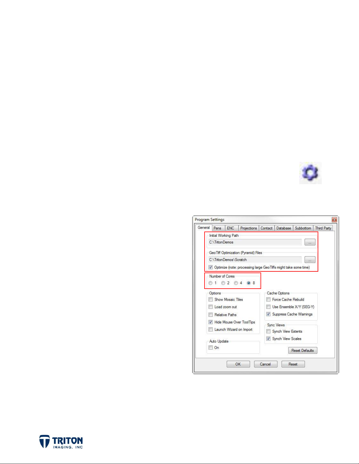
2.0 Settings
Before getting started it is best to review the
the settings are correct. The
selecting this toolbar button or by selecting the
View
menu.
Program Settings
Program Settings
2.1 File Paths
In the
file paths to set. The top one is called
Initial Working Path
for Perspective to look in for importing and
saving files.
The second file path option sets the location
for creating pyramid files which increases
the speed of zooming in and out of large
GeoTiffs. In addition to setting the file
General
settings tab there are two
sets the default folder
and verify
are accessed by either
Settings Info
option in the
path, it is important to also select the
Optimize
checkbox to activate this feature.
2.2 Number of Cores
Below the file paths is a section titled
(or threads) to use for working in Perspective. The default is 2 cores but the software will
accommodate up to 8 cores for faster performance.
Page 1
Number of Cores
for setting the number of cores
Page 5
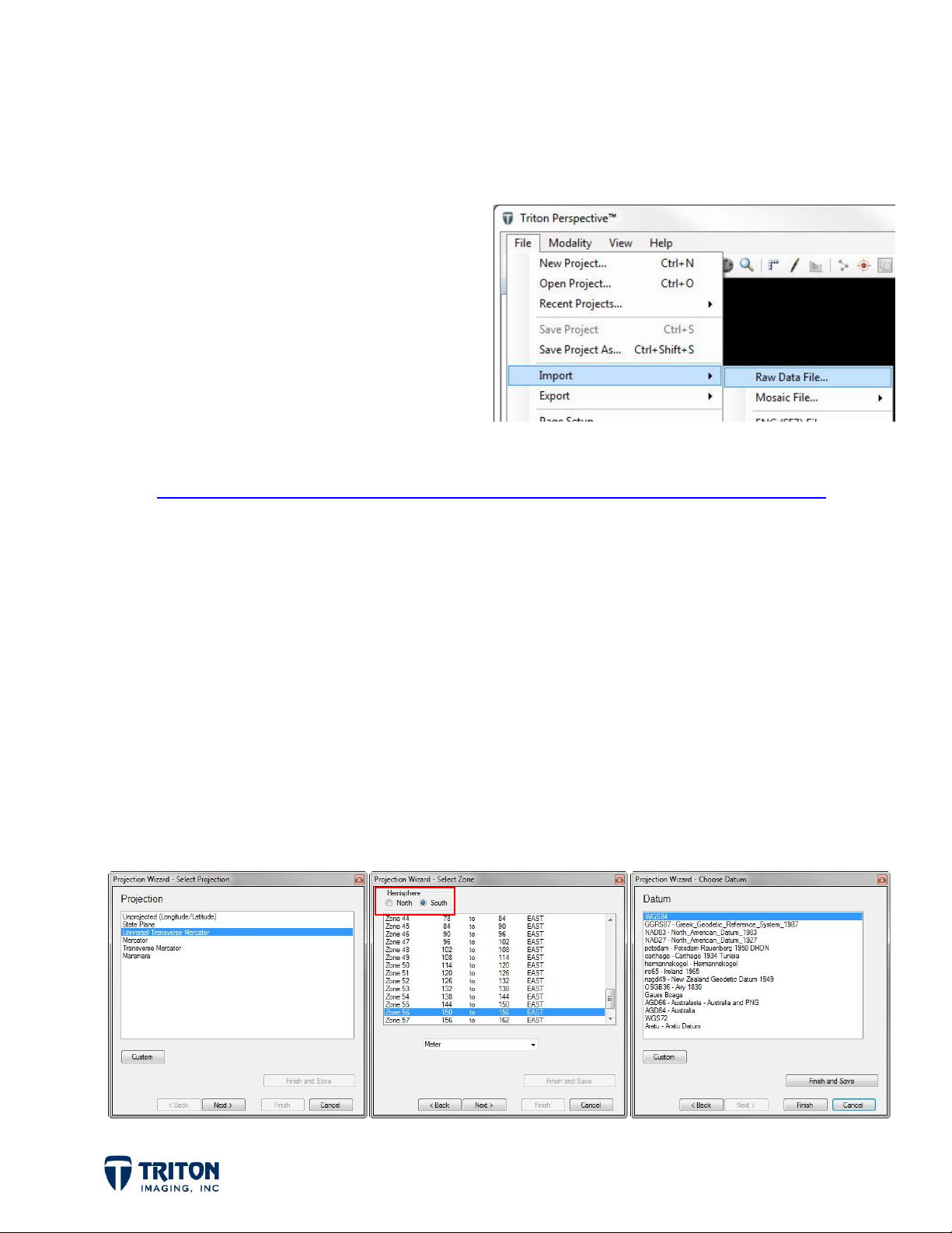
3.0 Import
3.1 File Import
To get started, the raw sidescan data files
need to be imported into Perspective using
the
Raw Data File
menu as shown in the capture to the right.
Please note that currently Perspective only
supports the XTF and SEGY file formats.
To convert from other formats we have a
several converters on our website at:
http://www.tritonimaginginc.com/site/content/support/downloads.htm#conv
option from the
Import
Some of the sonar manufacturers have their own converter so please contact us if you
have difficulty finding the converter you need.
Selecting the
A single file can be selected or multiple files for quickly importing multiple days of
recorded data.
Import/Raw Data File
option will open a file browser to locate raw data files.
3.2 Projection/Datum
If the data was collected in anything other than Latitude-Longitude, the Projection wizard
will launch and ask for the correct projection and datum to use as shown in the following
screen captures. Be sure to indicate which hemisphere, north or south!
Page 2
Page 6
If the projection used for the raw data files is not present in the standard lists, select
the Custom button to either manually enter the projection values or download a custom
projection string from:
http://spatialreference.org/
A custom datum can also be created by manually entering the datum values. For more
information on using the custom projection and datum options, open the
under
Projection
Program Settings
tab in the
Program Settings
. Note that the projection and datum can be preset in the
prior to importing data files or background imagery.
Help
file and look
3.3 Navigation
There are two important things that happen as the raw data is imported into Perspective.
The first is the creation of cache files for each imported line. This allows the original
data files to be unchanged during all the processing steps performed. The other is the
extraction of the navigation data from the raw data files
for display in the map view.
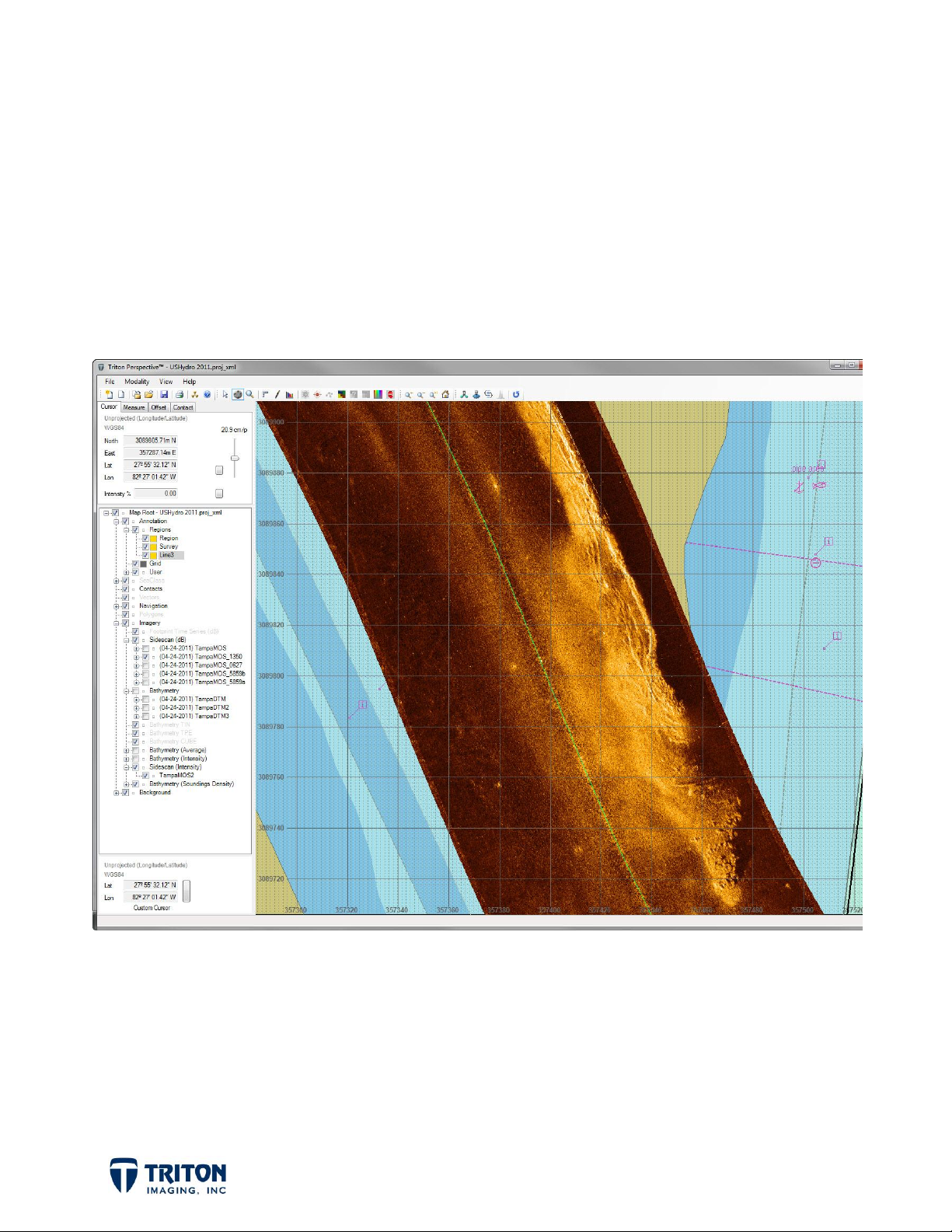
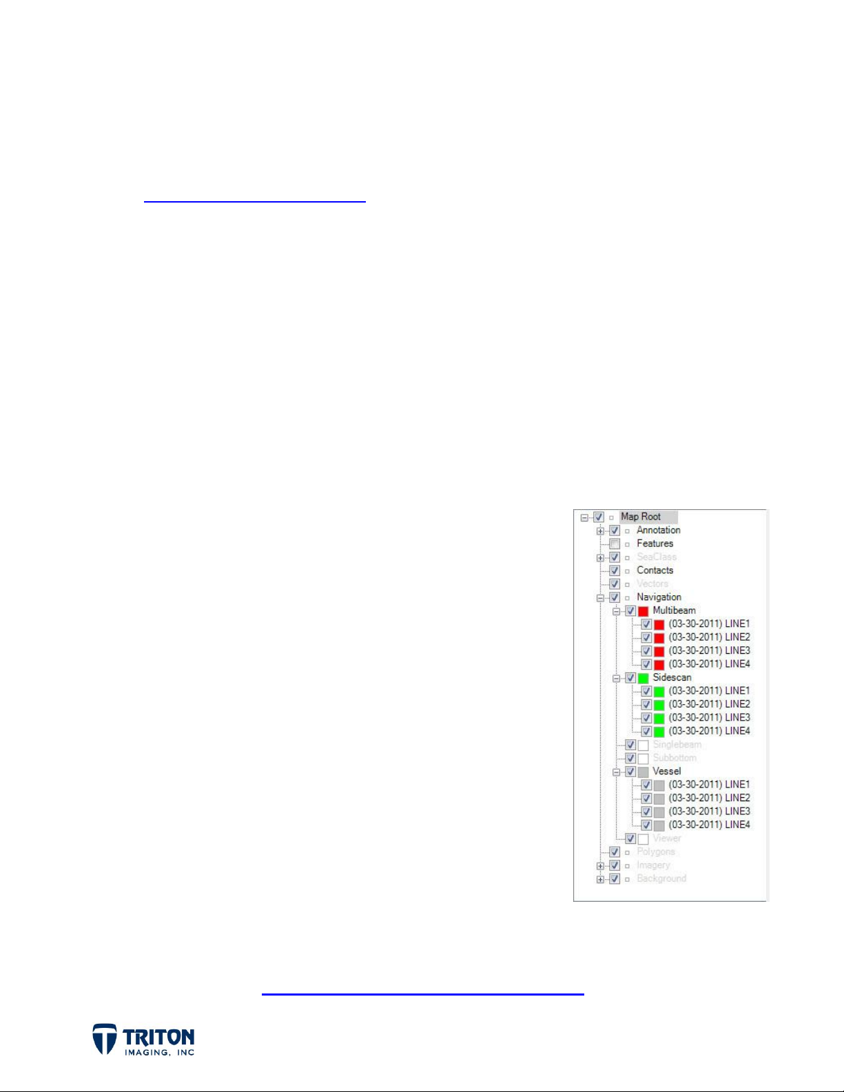
Perspective uses a GIS-like file tree structure for managing
imported data as shown to the right. The extracted
navigation is placed in the Navigation file tree node,
separated into different types depending on the data
present in the raw data file.
For example, navigation from an EdgeTech 4600 data file
will be split into three parts; one for the vessel position, one
for the sidescan navigation and another for the bathymetry
navigation. Although the raw navigation for the sidescan and
bathymetry from a combined sonar are identical, this is
important as it allows for the navigation to be processed
differently. It is often important to smooth the heading
for sidescan data but for bathymetry data it is preferred to
only remove navigation anomalies such as spikes in the data.
Navigation processing is a very important step for improving the quality of sidescan
mosaics. See Triton’s Perspective - Navigation Processing Guide for more information.
Page 3
Page 7
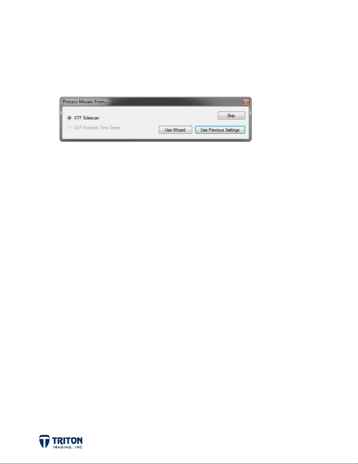
3.4 Import Processing Option
In the Program Settings, there is an option to launch the processing wizards upon
importing raw data. If this is selected, upon importing the raw data file(s), the dialog
shown below will pop-up asking if you would like to process the data at this time.
If you know the data has good navigation with uniform parallel beams, a good bottom track
from acquisition, and also that TVG corrections were made during data acquisition and
recorded to the raw data files, then the data can be processed during import with either
the
Use Wizard
or
Use Previous Settings
options.
The wizard remembers the previous settings used but allows the values to be adjusted.
However often when working in a consistent environment with the same sonar the only
setting that needs to be changed is the file name. Assuming the settings are good from
previous processing, then selecting the
mosaic without having to go through the wizard to select and adjust processing options.
To get the best results from processing sidescan data it often is best to first process the
navigation separately, then to review the raw data in the sidescan waterfall window to
verify the bottom tracking is good and to create a TVG curve if needed.
Use Previous Settings
option will create a sidescan
4.0 Review
4.1 Launch Waterfall Display
In order to verify and reset the bottom tracking and also to adjust the TVG, the data
must be viewed in the waterfall display which replays the raw XTF files. The waterfall
display can be launched a couple different ways. The easiest is by double-clicking on the
sidescan navigation line in the map view. This will open the waterfall at the location
selected and will put a circle on the navigation line indicating where along the line the
waterfall is displaying data for.
Page 4
Page 8
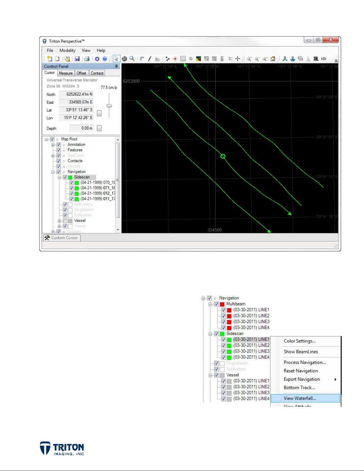
As the waterfall scrolls, the position in the map view updates to show the current location
of the waterfall display.
The other option to open the waterfall window
is right-clicking on the navigation line in the
file tree as shown to the right. This will
launch the waterfall at the beginning of the
navigation line but will still place the position
circle on the map display for tracking the
waterfall position.
This cursor tracking feature is very helpful
for interpretation allowing correlation of
features in the waterfall with same feature in
the mosaic or in other background data.
Page 5
Page 9
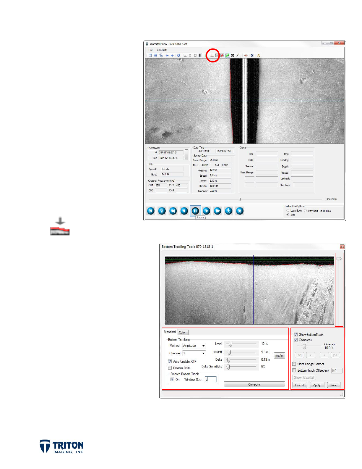
4.2 Bottom Tracking
To the right is an example of
the waterfall view showing
sidescan data collected using
a Klein 5000 sonar. The red
line in the waterfall window
shows that the selected file
already has bottom tracking
saved in the raw data file.
If the file is not bottom
tracked, or to either review
or reset the bottom tracking,
select the bottom tracking
toolbar button shown here.
Selecting this toolbar button will
open the window to the right for
setting or adjusting the bottom
tracking. Options available are
explained well in the
section of the
Important notes for using the
bottom tracking tool are
presented here:
1. The data is viewed
horizontally at the top of
Help
MosaicOne
file.
the window with an acrosstrack zoom slider bar and
along-track zoom "Compress" options.
2. The Color tab allows the user to improve the image quality in the bottom track view.
Page 6
Page 10

3. If the file includes both amplitude and depth information, then the bottom track
can be automatically extracted from the bathy nadir depth. Doing this may require
the user to apply a Bottom Track Offset to move the entire bottom track line up or
down by a specified value.
4. Auto Update XTF is the only place in Perspective that the user is able to overwrite
their raw data!. This option exists because bottom tracking a large survey can take
a considerable amount of time and once done it is best to save the new bottom
tracking information back to the raw data files instead of in cache files since cache
files are not always preserved with the raw data files for future work with the data.
5. The "Slant Range Correct" option applies the slant range correction typical for the
waterfall view to the bottom tracking display. Areas with portions of the water
column included in the slant-range corrected image will show up as black areas in the
data. This allows the user to QC the bottom track results, and to identify/repair
problem areas without having to return to the waterfall window to see the results.
An example of this is shown below.
Page 7
Page 11

Manual
Automatic
4.3 TVG Adjustments
Many modern sidescan sonars already account for TVG during acquisition and no
adjustments are required. However, when needed TVG corrections will greatly increase
the sidescan mosaic image quality. Prior to adjusting the TVG, it is important to slant
range correct the sidescan data in the waterfall view using the bottom track information.
This is accomplished by selecting the Slant Range toolbar button shown below.
There are two options for TVG, manual and automatic, launched by selecting one of the
toolbar buttons shown below:
To manually correct the TVG, note that it helps to place the TVG window such that the
range from 0 to Max spans the same section of the waterfall as shown below.
To adjust the TVG, click on the TVG line to create a node, then drag that node up (lighter)
or down (darker) to adjust the TVG at that location. Note it is possible to set the TVG
per channel or use one curve for all channels.
Page 8
Page 12

Below is the same example from the previous page but with the TVG manually adjusted:
Comparing the image above with the one on the previous page shows the attenuation loss
with increased range has been corrected for.
As mentioned above it is possible to use an automated routine for adjusting the TVG which
often has very good results. By default this will generate individual curves for each
channel.
Selecting the automatic TVG
button will open the dialog
shown right. Generally the
default values work well but it
is possible to select different
Process Types
Brightness, Contrast
Window Size
, and set the
and
. When finished,
click
Generate Curves
to
create the TVG curves.
Page 9
Page 13

Below is the same example again but with the TVG automatically adjusted:
It is interesting to note that the curve is similar to the one created manually but slightly
lower, increasing the overall gain level. Also note that sometimes with the automatic TVG
there is still a black stripe down the nadir. In these cases it is helpful to manually adjust
the automatically generated TVG curve in order to produce the results as shown below.
Page 10
Page 14

5.0 Process
5.1 Sidescan Mosaic Wizard
Once the navigation has been processed, the bottom track verified, and a TVG curve has
been created and saved, the sidescan data is ready to be processed. The
easiest method for launching the sidescan mosaic wizard is by selecting this
toolbar button. It is also possible to right-click on the
Imagery
Sidescan processing options are divided into six stages
Presented in this section is an example of parameters used for processing a Klein 5000
sidescan survey with a brief description of available options. Detailed explanations of the
options available in the mosaic
processing wizard are presented
file tree layer and select
1. Choose/Create Mosaic File
2. Choose Mosaic Settings
3. Select/Order Input Lines
4. Geometry Settings
5. Line and Channel Settings
6. Corrections and Filters
Create
.
Sidescan
node in the
in the
Help
5.1.1 Choose/Create Mosaic File
The first page of the sidescan
processing wizard allows the user
to choose a file name and location
for the mosaic to be generated.
The user can choose between
including all lines in one mosaic or
to create one mosaic per survey
line.
MosaicOne
file.
section of the
Page 11
Page 15
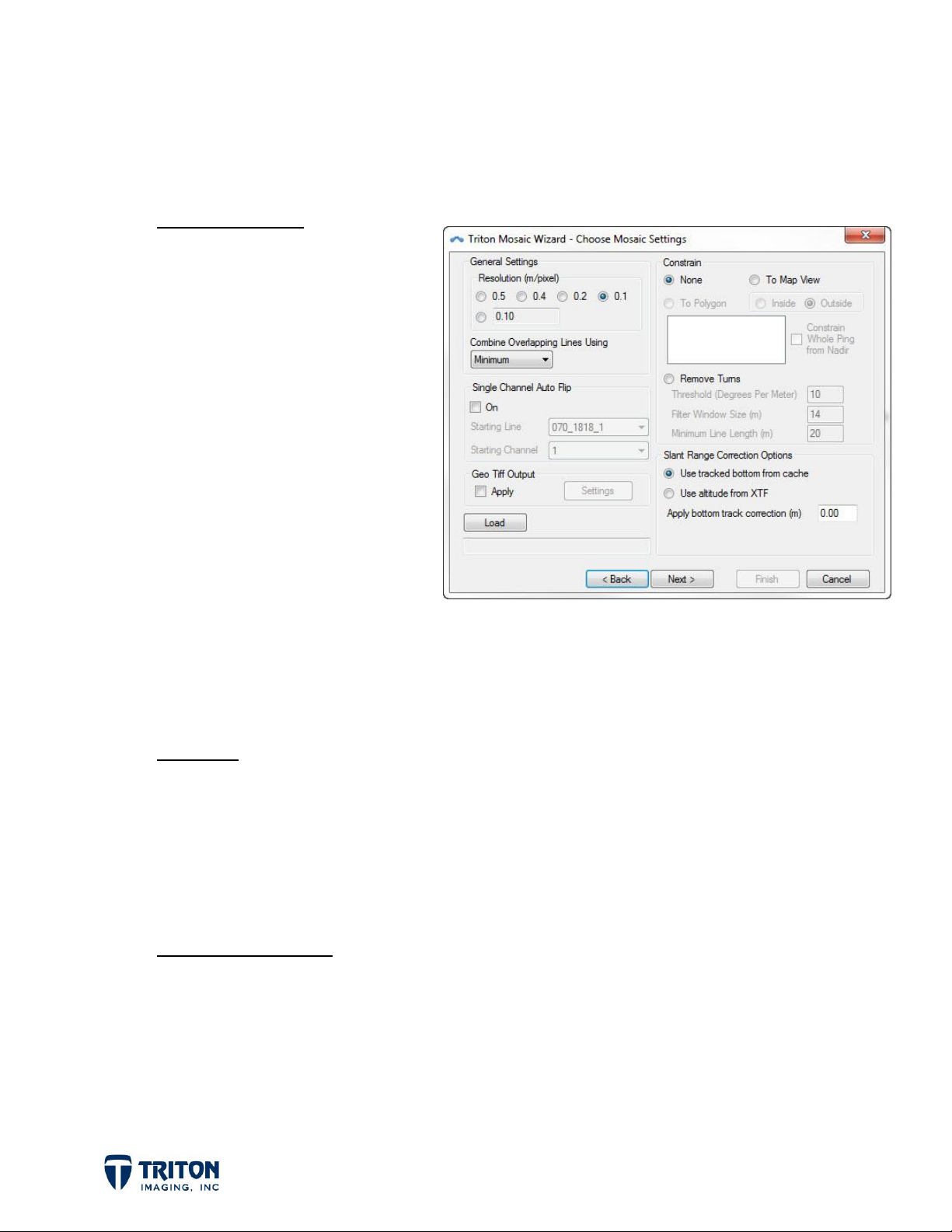
5.1.2 Choose Mosaic Settings
Settings pertaining to assembling the sidescan mosaic are located on page 2 of the
processing wizard. An overview of the options available is presented below.
General Settings
o
Resolution:
the mosaic resolution is set
(in meters).
o
Combine Overlapping Lines:
Methods for selecting
which cell value to use
where lines overlap.
o
Single Channel Auto-Flip:
This is where
Uses alternating channels
(port, starboard) to create
a mosaic with a consistent
shadow direction.
o
GeoTiff Output:
automatically export to GeoTiff formatted file(s).
Constrain
o Extent: Ability for limiting the extent of the mosaic based on either the map
view extent, a selected polygon
o Line Turns: Line curvature can be used to automatically remove turns from
the mosaic.
Slant Range Options
If selected, the generated sidescan mosaic file will
o
Source:
processed cache file.
o
Offset:
then that offset needs to be entered here.
The user choose the bottom track from the raw XTF file or from the
If a bottom track offset was applied in the Bottom Tracking Tool,
Page 12
Page 16

5.1.3 Select/Order Input Lines
This page allows the user to select
which lines to include in the
processing as shown below. Note
that the line order can also be
specified by right-clicking on a line
and selecting Move Up, Move Down,
or Move to Top.
5.1.4 Geometry Settings
Towfish Configuration: There are
two primary options for vessel
geometry for sidescan processing.
Traditionally, most sidescan sonars
are towed behind the survey vessel
with the layback amount stored on
the raw data file.
Note, if layback has already been
applied to the raw positions in the
XTF file or previously using
Perspective, then applying layback
again here will double the effect!
Also note that Perspective assumes
"layback" includes the towpoint
offsets from the GPS antenna. For
XTF files with 'layback=cable out'
without offsets included, be sure to add the towpoint offsets in both the X & Y directions.
Mounted/AUV Configuration: For AUV surveys and also for pole mounted interferometric
sidescan sonars, it is better to use offsets similar to bathymetry processing to account
for the separation between the sonar and motion reference unit (pitch) & heave sensors.
For manually entering offsets, pay close attention to the drawings for the sign convention
to use for the two options. Note that the Y-direction is positive to stern for towed
systems and positive towards the bow for mounted systems!
Page 13
Page 17

5.1.5 Line and Channel Settings
This page of the wizard is for
settings that apply on the individual
survey lines before they are
assembled into a mosaic.
Select Channel
port and starboard channels
can be selected or turned
off.
Clip Channel Ground Range
o
User Defined:
slider bars set the
These
amount of clipping to perform in either percentage or in meters. The outer
boundary can be set by clipping the maximum range or by setting the
maximum distance to use from the nadir position.
o
Clip based on Altitude:
the sonar altitude. According to NOAA specifications, the sonar altitude
needs to be within 8 to 20% of the ground range for the data to be
acceptable.
Fill Options
There are two primary fill methods which can be used separately or together.
1.
Between Pings
speed for the set ping rate .
2.
Grid
- Fill option based on values of adjacent cells generally used for
multibeam amplitude data and not true sidescan that has more than enough
- Fills along track data gaps resulting from too fast a vessel
Limits the ground range based on the percentage of
sample across track already compared to the along track direction. Options
for the Grid method include:
Grid Fill Dimensions
to fill from the closest known value.
Page 14
- for the Grid method, can set the number of cells
Page 18

o
Include Adjacent Cells
filled cell.
o
Non-Zero Shadow
amplitude for each grid cell in the shadow so imagery behind the mosaic does
not show through.
Channel Sampling Method
Both the Downsampling and Combine Overlap options refer to the method by
which overlapping data from within one line is handled.
o
Downsampling:
ping).
o
Combine Overlapping:
itself.
- uses the values in adjacent cells to calculate value of
- fills sidescan shadows where there is no data with a zero
refers to the across track element (sample to sample within a
refers to the merging of samples when a line overlaps
o
Each has the following options:
Average - the average pixel value is calculated and used
Maximum - the pixel with the highest value (maximum) is used
Minimum - the pixel with the lowest value (minimum) is used
RMS - Root Mean Square is a statistical measure of the magnitude of
pixel values. It is the square root of the mean of the squares of the
pixel values
Skip - does not apply this step, overlap is handled by input line order
Apply To
Allows the users to apply the same settings to all survey data lines or to apply
different setting to different lines.
o
All Checkbox:
processed. Leaving this checkbox not checked will enable users to set
different clipping and fill options for each line by selecting the lines from the
drop down list.
Page 15
selecting this will apply all setting on this page to all lines being
Page 19

5.1.6 Corrections and Filters
The last page of the sidescan
processing wizard is for correcting
position and gain loss in the mosaic.
Process Navigation
This section selects the
correct navigation to use for
creating the mosaic, with
three options available:
o
Process Navigation
processing is needed and
has not been done, then the top option allows the user to set the navigation
- If
processing parameters.
o
Use Processed Navigation -
option tells the processing algorithm to look in the cache for the navigation
values to use.
o Use Raw Navigation (from XTF) - This option is for data where the navigation
does not need to be processed and the values in the XTF files are good to use
for creating the mosaic. Generally this is only true for navigation processed
externally from Perspective and then inserted into the XTF file after it was
processed using scripts in MatLab or using another application.
Grid Corrections
If there is an existing DTM of the survey area, the topography can be used to
correct the mosaic in two ways:
o
Topography:
Applies 'position' corrections by using the changes in elevation
If processing has already been done, then this
in the DTM.
o
Angle of Incidence:
for the angle of incidence between the sidescan beam and the seafloor (still
is development!).
Page 16
Applies 'amplitude intensity' corrections by accounting
Page 20

Pitch Corrections
This option uses the 'pitch' value in the motion data (if available) to apply along
track position corrections. Options include:
o
From XTF:
an option here for setting an absolute angular offset
o
Static Offset:
to be inclined in the water at a fairly steady angle, a static pitch value can be
applied to the mosaic.
Latency
Check this box if there is a known latency and if the value is recorded to the
XTF files.
Reads the pitch value for each ping from the XTF file. There is
AIf the sidescan sonar was mounted at an angle or was known
TVG
The TVG tool allows the user to correct for gain loss in the sidescan record.
Checking this option will apply the loaded TVG curve.
Filters
There are two additional filters that users can apply to the raw data when
creating a sidescan mosaic.
o
Despeckle:
This filter is designed to remove interference and noise from
other sound sources seen in the sidescan record. The 'Threshold' sets the
amplitude of the "noise" that is acceptable. The 'Set Filter Extent' sets the
dimensions of the filter in the across track (samples) and along track (pings)
directions.
o
Moving Average:
This filter is designed to smooth the data to remove noise
from very turbid water or from poor quality sonars. The 'Moving Average'
Save
filter only works in the along track direction with the option to set the
number of pings to include.
The last option available is the ability to save all of the settings used to a file so
they can be recalled in the future.
Page 17
Page 21

5.2 Re-merge Mosaic
After the mosaic is created, it is possible to make a few
changes and have those changes incorporated into the mosaic
with the Re-Merge Mosaic option. This option is found by rightclicking on the mosaic file in the Imagery file tree.
When running the Re-Merge Mosaic option, the user will not
have any input and the same exact options used when the mosaic
was created will be used again. However there are three things
that can be changed with the Re-Merge Mosaic process without
needing to create a new mosaic:
1. Navigation Processing - If the user selected "Use
Processed Navigation" during the mosaic creation, then
the processing algorithm will read the navigation data
from the cache files where the processed navigation is
stored. In this case, selecting "Re-Merge Mosaic" will
use whatever navigation is currently written to the cache
files. Therefore, if the navigation has been re-processed
after the mosaic was created, the new processed
navigation will be written to the cache file and will be
used during the re-build process.
2. Bottom Tracking - Similarly to navigation processing, if during processing the user
selected "Use Tracked Bottom from Cache", then if the bottom tracking is re-done
after the mosaic is created when "Re-Merge Mosaic" is selected, the new bottom
track will be used.
3. TVG is the other change that can be made with the Re-Merge Mosaic option. As
long as the new TVG curve has the exact same name and is in the same folder as
when the mosaic was created, the new TVG curve will be applied during the re-build
process.
Once this option is selected, the mosaic file will be re-built using the new processed
navigation, bottom tracking and/or TVG curve, and then will be re-loaded into Perspective
for review and interpretation.
Page 18
Page 22

5.3 Other Processing Options
Presented here are a few optional processing tools:
5.3.1 Navigation Processing
The sidescan processing wizard only allows one pass at filtering the navigation. However,
for really bad navigation, either due to faulty equipment or overhead obstructions, this
may not be adequate to get good results from the sidescan data. To launch the
Navigation
5.3.2 Merge Lines
Some sonars or users automatically end their survey lines so they do not grow too large.
For processing, it is often preferred to have the small line segments merged into one line
segment. This can be done before creating a mosaic using the
5.3.3 Move Line
Move line allows lines within a mosaic to be moved relative to each other. This tool is great
for AUV data where there is often a navigation drift over time. Since the position of the
first survey line is generally the most accurate in an AUV survey, the subsequent lines can
be corrected by correlating features seen in the overlap area for both lines. To launch
the
Move Line
5.3.4 Add Lines
After a mosaic is created additional survey lines can be added using this tool. This is very
module, right-click on the
module, right-click on the sidescan file in the
Sidescan Navigation
file tree node.
Merge
Line toolbar button.
Sidescan Imagery
Process
tree node.
useful for multiple day surveys. As new lines are completed they can be processed and
added to the existing mosaic while the survey progresses. To launch the
right-click on the sidescan mosaic in the
5.3.5 Remove Lines
It is also possible to remove lines from an existing mosaic. This is found by right-clicking
on the sidescan mosaic in the
5.3.6 Single Channel Auto Flip
Found on page two of the mosaic processing wizard, this option will create a mosaic with a
single shadow direction, either port or starboard. It does this by selecting only the port
channel for one direction and only the starboard for the other. To do this there must be
at least 100% overlap between lines.
Page 19
Sidescan Imagery
Sidescan Imagery
file tree node.
file tree node.
Add Lines
tool,
Page 23

6.0 Enhance
There are two primary options for enhancing the appearance of the sidescan mosaics in
Perspective. These are adjustments to the
6.1 Color Settings
To open the
click on the mosaic file in the file
tree as shown to the right.
Selecting this will open the window
below.
Color Settings
, right-
Apart from changing the color bar as shown in the
window below, increasing the
the details in the mosaic.
Color Settings
and to the
Gamma
Histogram
can help bring out
.
6.2 Histogram
Changing the histogram adjusts
how the color map is spread
across the data range.
To open the
click on the mosaic file in the file
tree as shown to the right.
Histogram
Page 20
, right-
Page 24

Selecting the
Histogram
menu option will open the window below. The histogram and image
on the left have the default histogram while the histogram and image on the right have
had their histogram adjusted to bring out the details in the data.
Please note that these color and histogram options are also available in the waterfall
viewer and can have either the same settings or can be different from the mosaic color
and histogram settings.
By combining the color options with the histogram adjustments, subtle details in the data
can be enhanced for better interpretation.
Page 21
Page 25

7.0 Interpret
To assist with interpretation of the sidescan data Perspective has many added features
and toolsets. This section briefly describes some of the options available.
7.1 dB-based Imagery
To preserve the full dynamic range of the raw data file, Perspective keeps the data in dBs
instead of downsampling to fit a bitmap palette. This keeps
the maximum data range in the intact in the mosaic file.
Note also that as the cursor moves across the mosaic, the
percent relative intensity is displayed in the cursor
information display in the top left corner of the software.
7.2 Interactive Waterfall Display
The waterfall display in Perspective is closely linked to the map display. Shown below is
the Perspective map view with the waterfall position indicated by the green circle on the
navigation trackline. This position corresponds to the green horizontal line in the waterfall
viewer.
Page 22
Page 26

The sidescan waterfall accesses the raw XTF data and therefore preserves the raw data
quality. It can be launched by double-clicking on a sidescan navigation line, tracked while
scrolling by the circle moving along the navigation line, and moved around that line or to
another while scrolling by dragging it across the screen.
7.3 TargetOne
Integrated into Perspective is our full targeting
package. This allows for collection, classification and
display of targets seen in either the waterfall or in
the mosaics. If a target is identified in the waterfall
view, its position will be added to the map and vice
versa. Targets can be measured and saved to ASCII
or TIFF files.
7.4 SeaClass
Triton SeaClass is an advanced seabed segmentation/classification module that
automatically characterizes bottom types based on statistical properties of sidescan
mosaics or any GeoTiff loaded in the project. SeaClass is based on a multi-layer
perceptron supervised neural network.
The classification procedure consists of two stages: a learning stage and a classification
stage. Training is accomplished by the operator selecting areas in the mosaic of differing
bottom type (e.g. sand, rock, mud, etc.). Training of the classifier neural network then
proceeds through an automated statistical analysis of the selected samples and a
characterization of each
bottom type.
The classification stage is
a completely automated
process where the entire
mosaic image is segmented
into the different classes
as shown to the right.
Page 23
Page 27

8.0 Export
There are two primary exports for sidescan mosaics from Perspective. The main export is
to a GeoTiff, but it is also possible to export to a KML file.
8.1 GeoTiff
The sidescan mosaic can be exported to a GeoTiff by right-clicking on the mosaic file in
the file tree and selecting the GeoTiff export option. This will export a GeoTiff of the
entire sidescan mosaic with no other information overlain on the image.
The other GeoTiff export option is in the main
to as a
The other difference with the
extent of the map view.
Composite GeoTiff
since it contains everything that is displayed in the map view.
Composite GeoTiff
File
menu. This will export what we refer
is it will clip the mosaic to the current
8.2 KML
The sidescan mosaic can also be exported to a GoogleEarth KML file. This is accomplished
by right-clicking on the mosaic file in the file tree and selecting the KML export option.
This will export a KML file of the entire sidescan mosaic with no other information overlain
on the image.
Page 24
Page 28

9.0 Workflow
Step 1 - Launch Perspective: Start application and open project or start
new project
Step 2 - Check Settings: Verify maximum number of cores is selected and
if desired preset projection and datum for data and background
imports.
Step 3 - Import Data: Import raw data files into Perspective
Step 4 – Process Navigation: Process navigation from file tree and enable
Show Beamlines
to monitor results.
Step 4 - Review for TVG and Bottom Tracking: Verify data has good
bottom tracking and generate TVG curve if needed. This step can
be skipped if not needed.
Step 5 - Process Data: Use processing wizard to generate a sidescan
mosaic.
Step 6 - Enhance Imagery: Use the color settings and histogram
adjustments to bring out subtle details in the sidescan data.
Step 7 - Data Interpretation: Use advanced tools and fusion with other
data sets for sidescan data interpretation.
Step 8 - Export Results: Export sidescan mosaic files, targets, and seafloor
classification results.
Step 9 - Collect more data!
Page 25
 Loading...