

Page 1

®
Applications Guide
PID Control
in Tracer Controllers
CNT-APG002-EN
Page 2

®
Applications Guide
PID Control
in Tracer Controllers
CNT-APG002-EN
October 2001
Page 3

PID Control in Tracer Controllers
This manual and the information in it are the property of American Standard Inc. and shall not be used or reproduced in whole or in
part, except as intended, without the written permission of American Standard Inc. Since The Trane Company has a policy of continuous product improvement, it reserves the right to change design and specification without notice.
The Trane Company has tested the system described in this manual. However, Trane does not guarantee that the system contains no
errors.
The Trane Company reserves the right to revise this publication at any time and to make changes to its content without obligation to
notify any person of such revision or change.
The Trane Company may have patents or pending patent applications covering items in this publication. By providing this document,
Trane does not imply giving license to these patents.
The following are trademarks or registered trademarks of The Trane Company: Tracer, Tracer Summit, and Trane.
™
Printed in the U.S.A.
© 2001 American Standard Inc. All rights reserved.
Page 4

®
Contents
Chapter 1 Overview of PID control. . . . . . . . . . . . . . . . . . . . . . 1
What PID loops do . . . . . . . . . . . . . . . . . . . . . . . . . . . . . . . . . . . . . . . . . . . 1
How PID loops work . . . . . . . . . . . . . . . . . . . . . . . . . . . . . . . . . . . . . . . . . . 2
PID calculations. . . . . . . . . . . . . . . . . . . . . . . . . . . . . . . . . . . . . . . . . . . . . . 3
Proportional calculation. . . . . . . . . . . . . . . . . . . . . . . . . . . . . . . . . . . . 3
Integral calculation. . . . . . . . . . . . . . . . . . . . . . . . . . . . . . . . . . . . . . . . 4
Derivative calculation . . . . . . . . . . . . . . . . . . . . . . . . . . . . . . . . . . . . . 5
Velocity model . . . . . . . . . . . . . . . . . . . . . . . . . . . . . . . . . . . . . . . . . . . . . . 7
Chapter 2 PID settings. . . . . . . . . . . . . . . . . . . . . . . . . . . . . . . . 9
Throttling range . . . . . . . . . . . . . . . . . . . . . . . . . . . . . . . . . . . . . . . . . . . . . 9
Gains . . . . . . . . . . . . . . . . . . . . . . . . . . . . . . . . . . . . . . . . . . . . . . . . . . . . . 10
Calculating the gains . . . . . . . . . . . . . . . . . . . . . . . . . . . . . . . . . . . . . . . . .11
Sampling frequency . . . . . . . . . . . . . . . . . . . . . . . . . . . . . . . . . . . . . . . . . 12
Calculating the sampling frequency . . . . . . . . . . . . . . . . . . . . . . . . . . . . 14
Action. . . . . . . . . . . . . . . . . . . . . . . . . . . . . . . . . . . . . . . . . . . . . . . . . . . . . 17
Direct action . . . . . . . . . . . . . . . . . . . . . . . . . . . . . . . . . . . . . . . . . . . . 17
Reverse action . . . . . . . . . . . . . . . . . . . . . . . . . . . . . . . . . . . . . . . . . . 17
Determining the action . . . . . . . . . . . . . . . . . . . . . . . . . . . . . . . . . . . 18
Error deadband . . . . . . . . . . . . . . . . . . . . . . . . . . . . . . . . . . . . . . . . . . . . . 19
Typical applications . . . . . . . . . . . . . . . . . . . . . . . . . . . . . . . . . . . . . . 19
Adjusting error deadband for modulating outputs. . . . . . . . . . . . . 20
Adjusting error deadband for staged outputs . . . . . . . . . . . . . . . . . 20
Other PID settings. . . . . . . . . . . . . . . . . . . . . . . . . . . . . . . . . . . . . . . . . . . 21
Chapter 3 Programming PID loops. . . . . . . . . . . . . . . . . . . . . 23
Programming in PCL . . . . . . . . . . . . . . . . . . . . . . . . . . . . . . . . . . . . . . . . 23
Programming in TGP . . . . . . . . . . . . . . . . . . . . . . . . . . . . . . . . . . . . . . . . 26
CNT-APG002-EN iii
Page 5

®
Contents
Chapter 4 Applications . . . . . . . . . . . . . . . . . . . . . . . . . . . . . . 29
Discharge-air temperature control. . . . . . . . . . . . . . . . . . . . . . . . . . . . . . 29
Building pressure control . . . . . . . . . . . . . . . . . . . . . . . . . . . . . . . . . . . . . 32
Cascade control—first stage. . . . . . . . . . . . . . . . . . . . . . . . . . . . . . . . . . . 34
Staging cooling-tower fans . . . . . . . . . . . . . . . . . . . . . . . . . . . . . . . . . . . 37
Setting up the PID loop. . . . . . . . . . . . . . . . . . . . . . . . . . . . . . . . . . . . 37
Determining the staging points . . . . . . . . . . . . . . . . . . . . . . . . . . . . . 42
Chapter 5 Troubleshooting . . . . . . . . . . . . . . . . . . . . . . . . . . . 45
Troubleshooting procedure . . . . . . . . . . . . . . . . . . . . . . . . . . . . . . . . . . . 45
Tips for specific problems . . . . . . . . . . . . . . . . . . . . . . . . . . . . . . . . . . . . 46
Changing the sampling frequency . . . . . . . . . . . . . . . . . . . . . . . . . . 46
Changing the gains. . . . . . . . . . . . . . . . . . . . . . . . . . . . . . . . . . . . . . . 46
Examples . . . . . . . . . . . . . . . . . . . . . . . . . . . . . . . . . . . . . . . . . . . . . . . . . . 47
Chapter 6 Frequently asked questions . . . . . . . . . . . . . . . . . 51
Appendix A The math behind PID loops . . . . . . . . . . . . . . . . . 55
Velocity model formula. . . . . . . . . . . . . . . . . . . . . . . . . . . . . . . . . . . . . . . 55
Proportional control formula . . . . . . . . . . . . . . . . . . . . . . . . . . . . . . . . . . 55
Glossary . . . . . . . . . . . . . . . . . . . . . . . . . . . . . . . . . 57
Index . . . . . . . . . . . . . . . . . . . . . . . . . . . . . . . . . . . . 61
iv CNT-APG002-EN
Page 6

®
Chapter 1
Overview of PID control
This guide will help you set up, tune, and troubleshoot proportional, integral, derivative (PID) control loops used in Tracer controllers. These controllers include the Tracer MP580/581, AH540/541, and MP501
controllers. This chapter provides an overview of PID control.
What PID loops do
A PID loop is an automatic control system that calculates how far a measured variable is from its setpoint and, usually, controls an output to
move the measured variable toward the setpoint. The loop performs proportional, integral, and derivative (PID) calculations to determine how
aggressively to change the output.
The goal of PID control is to reach a setpoint as quickly as possible without overshooting the setpoint or destabilizing the system. If the system is
too aggressive, it will overshoot the setpoint as shown in Figure 1. If it is
not aggressive enough, the time to reach the setpoint will be unacceptably
slow.
Figure 1: The effects of PID aggressiveness
Too aggressive (overshoot)
Setpoint
Ideal response
Measured variable
Initial point
In the heating, ventilating, and air-conditioning (HVAC) industry, PID
loops are used to control modulating devices such as valves and dampers.
Some common applications include:
Too slow
Time
• Temperature control
• Humidity control
• Duct static pressure control
• Staging applications
CNT-APG002-EN 1
Page 7
®
Chapter 1 Overview of PID control
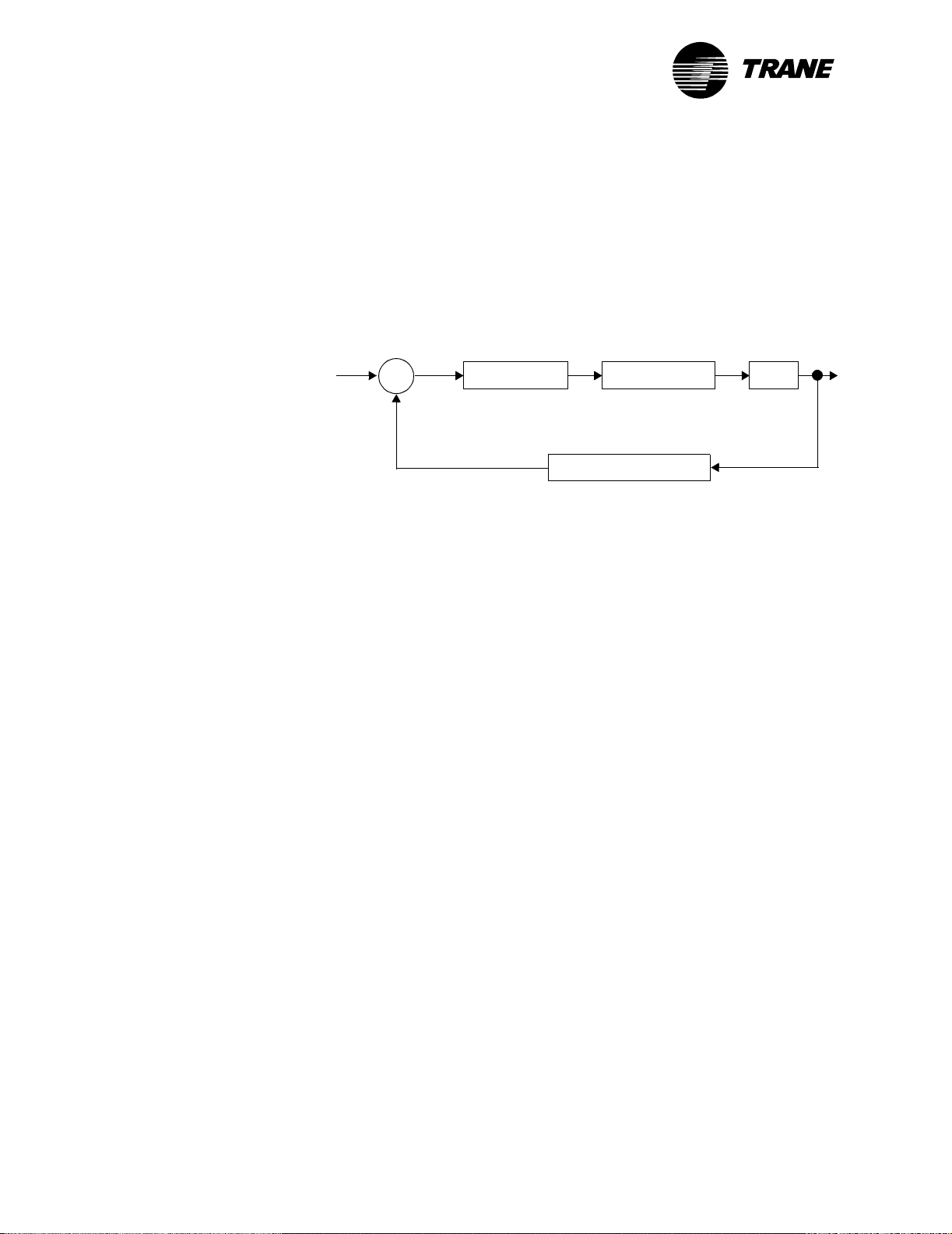
How PID loops work
A PID loop performs proportional, integral, and derivative calculations to
calculate system output. Figure 2 illustrates how a typical PID loop
works. The sigma (Σ) symbol indicates that a sum is being performed. The
plus (+) symbol indicates addition, and the minus (–) symbol indicates
subtraction.
Figure 2: PID loop
+
Setpoint
Error
Σ
–
Measured variable
(process variable)
PID calculation
HVAC equipment
Conversion function
Plant
In an HVAC system, the controller uses a PID calculation to change the
output of mechanical equipment to maintain some setpoint. For example,
if a space is too cold, the PID calculation controls an actuator to open a
hot-water valve some amount, increasing the discharge-air temperature
to heat the space.
In classic PID control systems, the controller reacts to a comparison
between a setpoint and a measured variable (also called the process variable). The setpoint is often a user-defined setting, such as a room temperature setpoint. The measured variable is the controlled element, in this
case the current room temperature.
The difference between the setpoint and the measured variable is called
the error, which is the value used to calculate system output. The error is
defined as:
Error = setpoint – measured variable
For example, if a room temperature setpoint is 75°F (23.9°C) and the
actual temperature is 65°F (18.3°C), then the error is 10°F (5.6°C).
The PID calculation uses the error to calculate an output that moves the
measured variable toward the setpoint as quickly as possible without
overshooting the setpoint. The output typically controls the position of an
actuator over a range of 0% to 100%. In the example above, an actuator
would open a hot-water valve some amount to increase the room temperature by 10°F (5.6°C).
The plant is the physical system, such as a room or a duct, that contains
the controlled element (the measured variable). The conversion function
converts the measured variable to the same units as the setpoint. For
example, a thermistor measures space temperature in terms of resistance, which is then converted to a temperature by the analog input of the
controller.
2 CNT-APG002-EN
Page 8
PID calculations
®
PID calculations
A PID loop performs three calculations: the proportional calculation, the
integral calculation, and the derivative calculation. These calculations
are independent of each other but are combined to determine the
response of the controller to the error.
Proportional calculation
The proportional calculation responds to how far the measured variable is
from the setpoint. The larger the error, the larger the output of the calculation. The proportional calculation has a much stronger effect on the
result of the PID calculation than either the integral or derivative calculations. It determines the responsiveness (or aggressiveness) of a control
system. Though some systems use only proportional control, most Trane
controllers use a combination of proportional and integral control.
Proportional-only control (a method of control that does not use the integral and derivative contributions) is traditionally used in pneumatic controllers. It may be used in staging applications because it can be simpler
to manage than full PID control. The programmable control module
(PCM) and the universal programmable control module (UPCM) assume
proportional-only control when the integral and derivative gains are set
to zero. Tracer MP580/581 controllers have a unique setting for proportional-only control. Figure 3 illustrates proportional-only control.
Figure 3: Proportional-only control
Setpoint
Measured
variable
+
Σ
–
Error(n)
Proportional gain
Proportional bias
Conversion function
System
+
output
Σ
+
One difference between proportional-only control and classic PID control
is the use of proportional bias. The proportional bias becomes the output
when the error is zero. Thus, you can use the proportional bias to calibrate a controller to some known output. Figure 4 on page 4 shows the
effect of proportional bias on PID output. Notice that when the error is
zero, the output is equal to the proportional bias.
Note:
The integral calculation automates the process of setting proportional bias. In proportional-only control, the proportional
bias lets you decide what the output should be when the error is
zero; in PID control, the integral calculation maintains the current output when the error is zero (see “Integral calculation” on
page 4).
CNT-APG002-EN 3
Page 9
®
Chapter 1 Overview of PID control
Figure 4: The effects of proportional bias on system output
Proportional bias = 75
Proportional bias = 50
Controller output (%)
Proportional bias = 25
Error
Integral calculation
The integral calculation responds to the length of time the measured variable is not at setpoint. The longer the measured variable is not at setpoint, the larger the output of the integral calculation.
The integral calculation uses the sum of past errors to maintain an output when the error is zero. Line 1 in Figure 5 on page 5 shows that with
proportional-only control, when the error becomes zero, the PID output
also goes to zero (assuming a proportional bias of zero). Line 2 shows the
integral output added to the proportional output. Because the integral
calculation is the sum of past errors, the output remains steady rather
than dropping to zero when the error is zero. The benefit of this is that
the integral calculation keeps the output at an appropriate level to maintain an error of zero.
4 CNT-APG002-EN
Page 10

®
Figure 5: Integral output added to proportional output
PID calculations
Error ≠ 0
Proportional + integral
output
2
Output
1
Proportional-only
output
Time
Error = 0
Proportional + integral
output when proportional
output has gone to zero
The value of the integral calculation can build up over time (because it is
the sum of all past errors), and this built-up value must be overcome
before the system can change direction. This prevents the controller from
over-reacting to minor changes, but can potentially slow down the
response.
One drawback to integral control is the problem of integral windup. Integral windup occurs when the sum of the past errors is too great to overcome. This can happen when the HVAC equipment does not have enough
power to reach the setpoint; the integral windup only increases as the
equipment struggles to reach the setpoint. To minimize the problem of
integral windup, Trane controllers use a method of PID control known as
the velocity model, which is described in “Ve l o city m o de l” on page 7.
Derivative calculation
The derivative calculation responds to the change in error. In other
words, it responds to how quickly the measured variable is approaching
setpoint. The derivative calculation can be used to smooth an actuator
motion or cause an actuator to react faster.
However, derivative control has several disadvantages:
• It can react to noise in the input signal.
• Setting derivative control requires balancing between two extremes;
too much derivative gain and the system becomes unstable, too little
and the derivative gain has almost no effect.
• The lag in derivative control makes tuning difficult.
• Large error deadbands, common in HVAC applications, render deriv-
ative control ineffective.
CNT-APG002-EN 5
Page 11
®
Chapter 1 Overview of PID control
Because of these disadvantages, derivative control is rarely used in HVAC
applications (with the exception of steam valve controllers and static
pressure control).
Derivative control can affect the output in two ways: it slows the output if
the derivative gain is negative and increases the output if the derivative
gain is positive.
Slowing (or smoothing) the actuator motion, sometimes known as
dynamic braking, can help if there are many quick changes in the input
signal. For example, a robot arm moves quickly in mid-motion, but the
derivative calculation slows it down at the end of the motion.
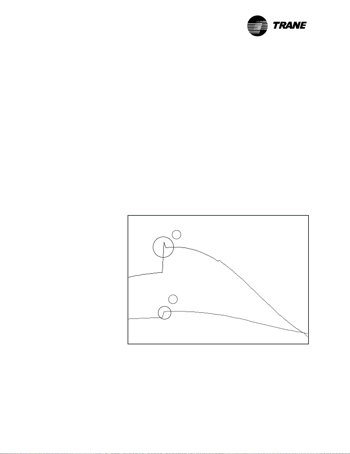
The opposite effect occurs when the derivative gain is positive. The output reacts faster to a change in error, resulting in a steeper climb or
descent to setpoint. The circled areas in Figure 6 illustrate this effect.
Line 1 shows the error without a derivative gain. Line 2 shows the error
with a positive derivative gain. The circled sections show what happens
during a rapid change in error. Note the spike in line 2 as the system
recovers from the effect of derivative control during a sharp change in
error. The spike indicates a forceful actuator motion, which is useful for
applications such as controlling steam valves.
Figure 6: The effect of positive derivative gain
Proportional gain ≠ 0
2
Derivative gain > 0
Output
Proportional gain
1
Derivative gain = 0
≠ 0
Time
6 CNT-APG002-EN
Page 12
Velocity model
®
Velocity model
Trane controllers use a type of PID control known as the velocity model.
The velocity model minimizes the problem of integral windup, which
occurs when the sum of past errors in the integral calculation is too great
to allow the controller to change the output at one of the extremes (see
“Integral calculation” on page 4).
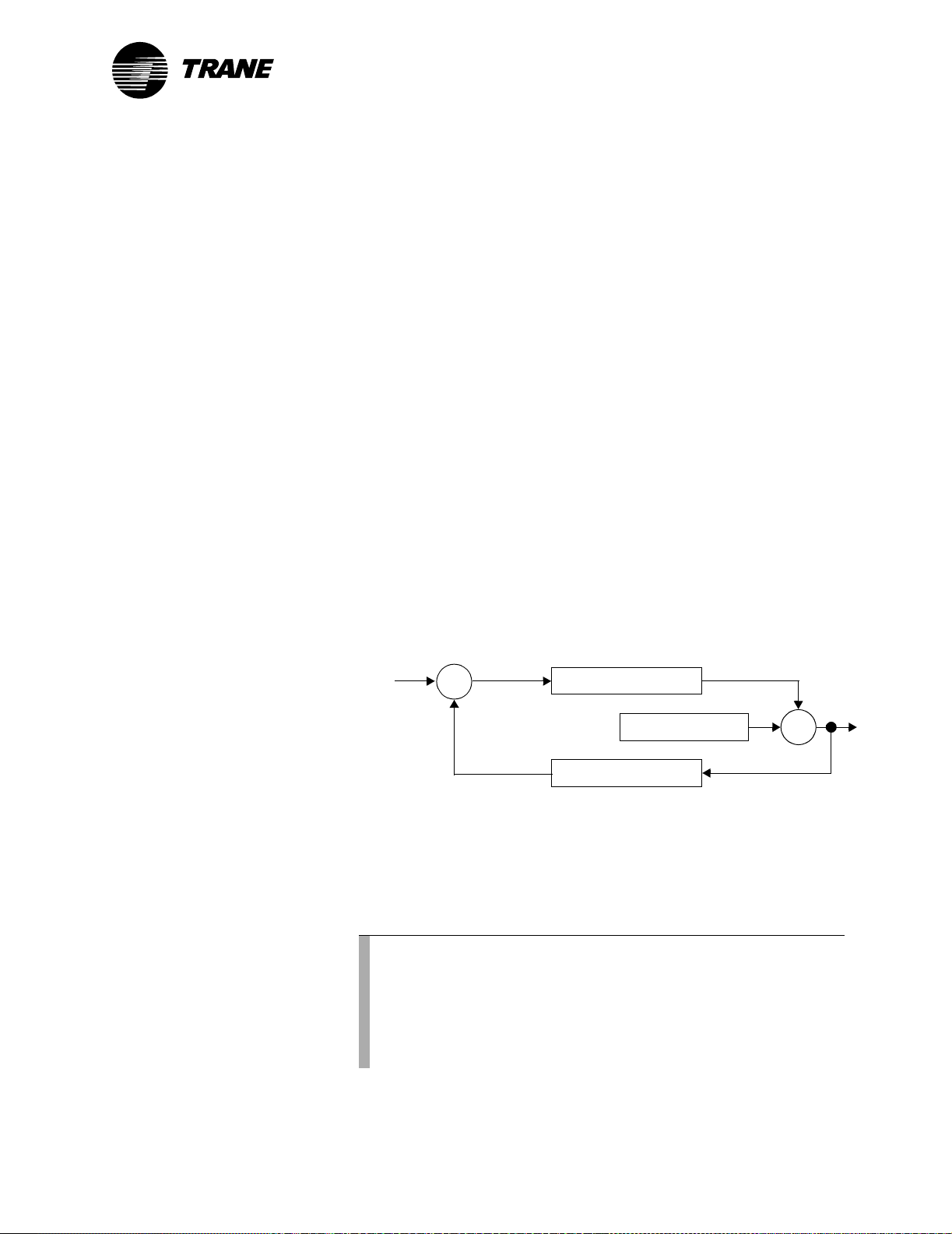
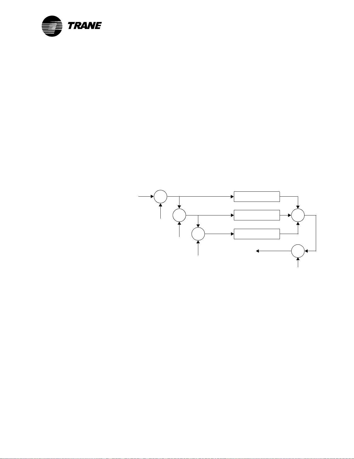
The velocity model, illustrated in Figure 7, gets its name from the fact
that the proportional gain affects the change in error (or error velocity)
instead of the error, as in a classic PID model. In the velocity model, the
error is multiplied by the integral gain, and the change in error is multiplied by the proportional gain. When the error gets close to zero, the
change in error gets close to zero as well. So both the integral and proportional gains are multiplied by a number close to zero. This forces the output of the PID calculation to stop changing when the error becomes zero,
minimizing (but not eliminating) integral windup.
Figure 7: Velocity model
Setpoint
+
Measured
variable
Error(n)
Σ
–
+
Error(n-1)
∆error(n-1)
Σ
∆error(n)
–
+
Σ
–
∆2error(n)
Integral gain
Proportional gain
Derivative gain
PID output
PID output(n-1)
+
∆output(n)
Σ
+
+
+
Σ
+
CNT-APG002-EN 7
Page 13

®
Chapter 1 Overview of PID control
8 CNT-APG002-EN
Page 14
®
Chapter 2
PID settings
This chapter describes some of the key variables used to set up and tune
PID loops. The variables discussed here are:
• Throttling range
• Gain
• Sampling frequency
• Action
• Error deadband
Throttling range
The throttling range is the amount of error it takes to move the output of
a system from its minimum to its maximum setting. For example, a throttling range of 4°F (2.2°C) means that a controller fully opens or closes an
actuator when the error is
Figure 8. Note how the controller response (actuator position) lags behind
the space temperature.
±2°F (1.1°C) or greater, as illustrated in
Figure 8: Throttling range
Setpoint = 75°F
Space temperature (°F)
Actuator position
Actuator position (%)
Space temperature
Throttling range = 4°F
Time
CNT-APG002-EN 9
Page 15
®
Chapter 2 PID settings
The throttling range determines the responsiveness of a control system to
disturbances. The smaller the throttling range, the more responsive the
control. You cannot directly program the throttling range in Tracer controllers; rather, the throttling range is used to calculate the gains.
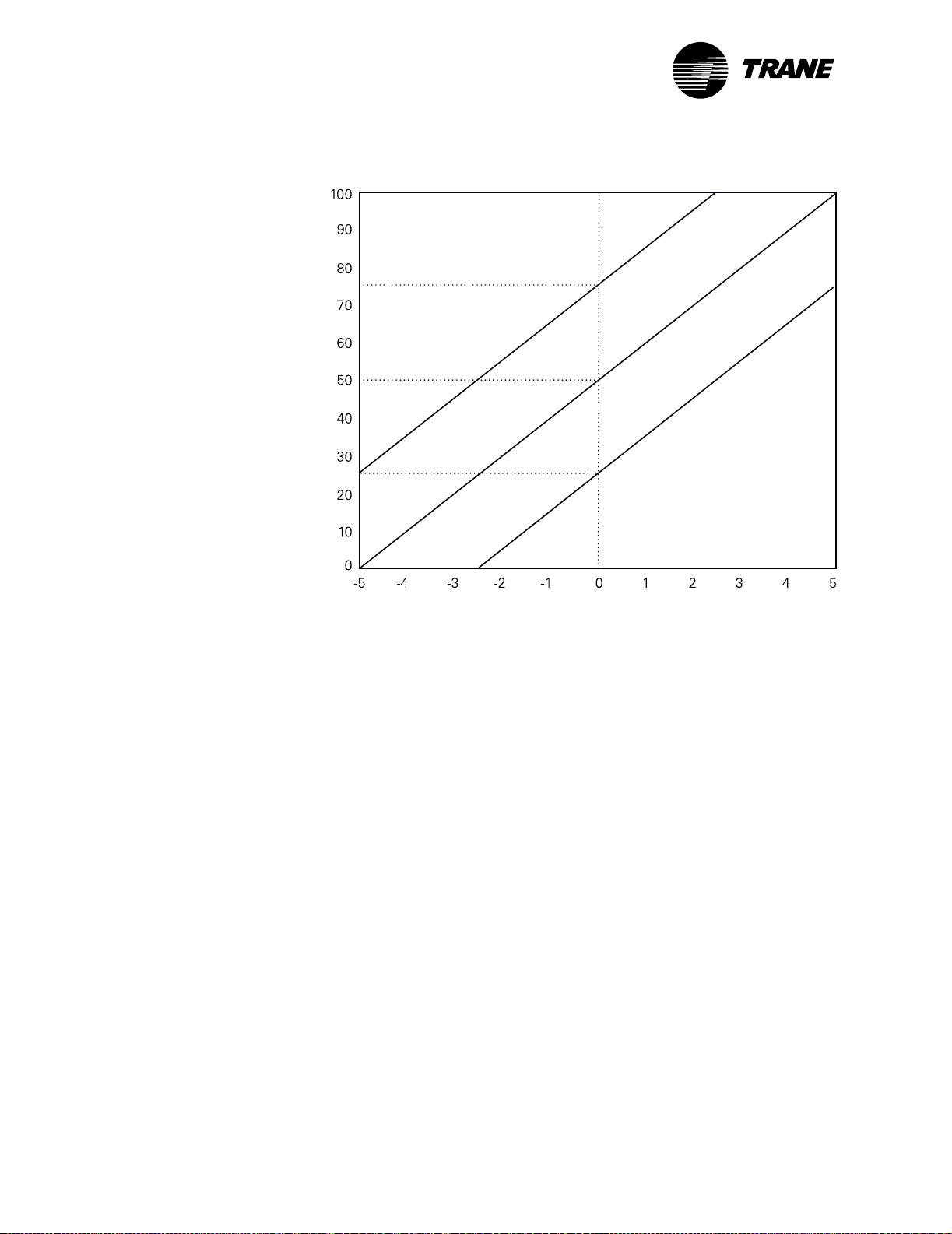
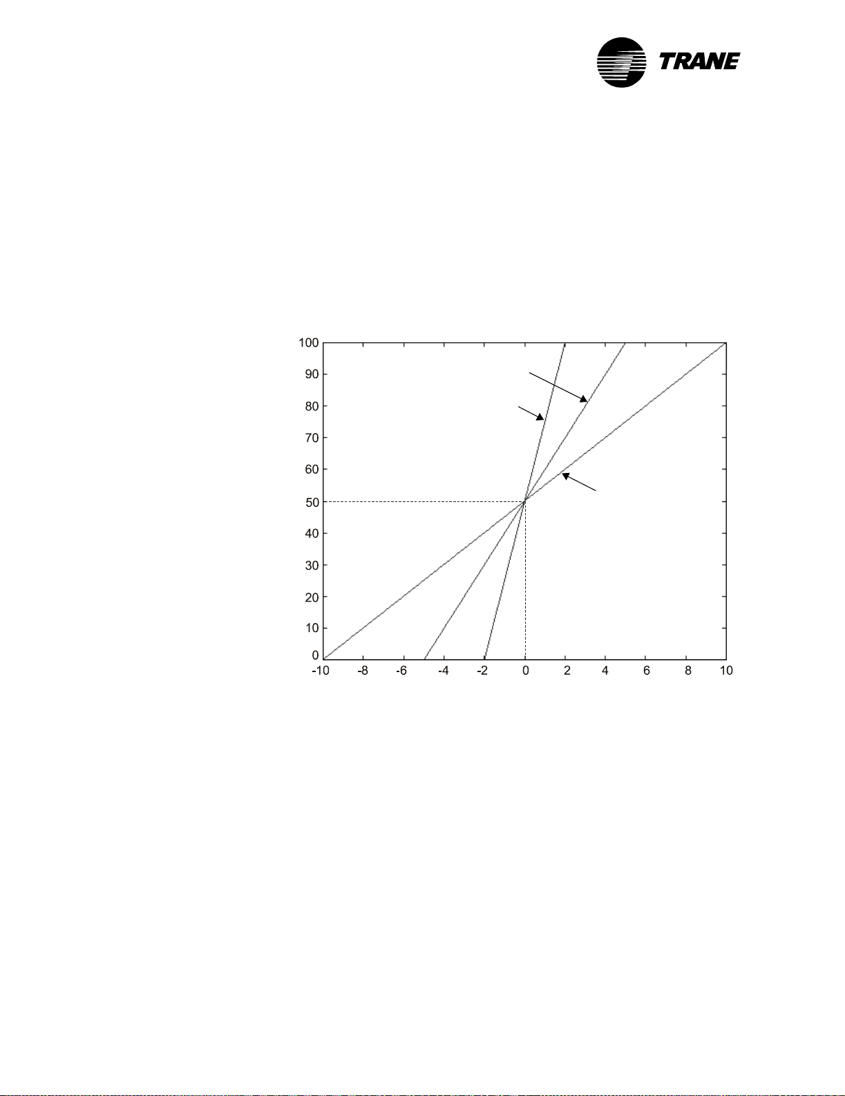
Figure 9 shows that as the throttling range increases, the potential error
becomes larger. When the output is at 0% or 100%, the error is equal to
one-half of the throttling range. For example, with a 10° throttling range,
the potential error is 5° from the setpoint (though the error could
exceed 5°).
Figure 9: Throttling range and error with proportional bias = 50
Throttling range = 10
Throttling range = 4
Throttling range = 20
Controller output (%)
Error
Gains
Gains, which are calculated from the throttling range, determine how fast
a measured variable moves toward the setpoint. The larger the gains, the
more aggressive the response. The proportional, integral, and derivative
calculations each have an associated gain value. The error, the sum of
past errors, and the change in error are multiplied by their associated
gains to determine the impact that each has on the output.
10 CNT-APG002-EN
Page 16

®
Calculating the gains
Table 1 shows recommended initial values for the proportional and integral gains for several applications. Most applications do not require a
derivative contribution, so the derivative gain is not shown. We recommend using a ratio of 4:1 between the proportional and integral gains, so
the proportional gain should be four times as large as the integral gain.
You may need to modify the values shown in Table 1 when tuning a PID
loop, but try to maintain the 4:1 ratio.
Table 1: Starting gain values for applications
Calculating the gains
Application Output Throttling range
Discharge-air cooling Valve position 0–100% 20.0°F (11.1°C) 4.0 (8.0) 1.0 (2.0)
Discharge-air heating Valve position 0–100% 40.0°F (22.2°C) 2.0 (4.0) 0.5 (1.0)
Space temperature Discharge setpoint
50–10 0°F (10–37.8°C)
Duct static pressure Inlet guide vane or variable-frequency
drive (VFD) position 0–100%
Building static
pressure
Discharge-air cooling Electric/pneumatic
Inlet guide vane or variable-frequency
drive (VFD) position 0–100%
5.0–15.0 psi (34–103 kPa)
2.0°F (1.1°C) 20.0 (20.0) 5.0 (5.0)
2.0 in. wc (0.5 kPa) 40.0 (160) 10.0 (40.0)
20.0 in. wc (5.0 kPa) 4.0 (8.0) 1.0 (2.0)
20.0°F (11.1°C) 0.4 (4.0) 0.1 (1.0)
Proportional
gain
Integral
gain
You can also calculate proportional and integral gains using the following
calculations:
Proportional gain
Integral gain
0.80 output range×
--------------------------------------------------------=
throttling range
0.20 output range×
--------------------------------------------------------=
throttling range
The proportional gain is scaled by a factor of 0.80, so it contributes 80% of
the final output. The integral gain contributes 20% of the final output.
Example
In a duct static pressure system, an actuator can move the inlet guide
vanes of an air handler from 0–100%, so the output range is 100. We want
a throttling range of 2.0 in. wc (so a change in pressure of 2.0 in. wc or
more will drive the output from 0–100% or vice versa). The calculations
look like this:
Proportional gain
0.80 output range×
------------------------------------------------------
throttling range
0.80 100×
----------------------------
2.0 in. wc
40===
Integral gain
0.20 output range×
------------------------------------------------------
throttling range
0.20 100×
----------------------------
2.0 in. wc
10===
So based on the desired throttling range of 2.0 in. wc, the initial proportional gain is 40 and the integral gain is 10.
CNT-APG002-EN 11
Page 17
®
Chapter 2 PID settings
Figure 10: Sampling too slowly
Sampling frequency
The sampling frequency is the rate at which the input signal is sampled
and the PID calculations are performed. Using the right sampling frequency is vital to achieving a responsive and stable system. Problems can
arise when the sampling frequency is too slow or too fast in comparison to
time lags in the system.
Sampling too slowly can cause an effect called aliasing in which not
enough data is sampled to form an accurate picture of changes in the
measured variable. The system may miss important information and
reach the setpoint slowly or not at all.
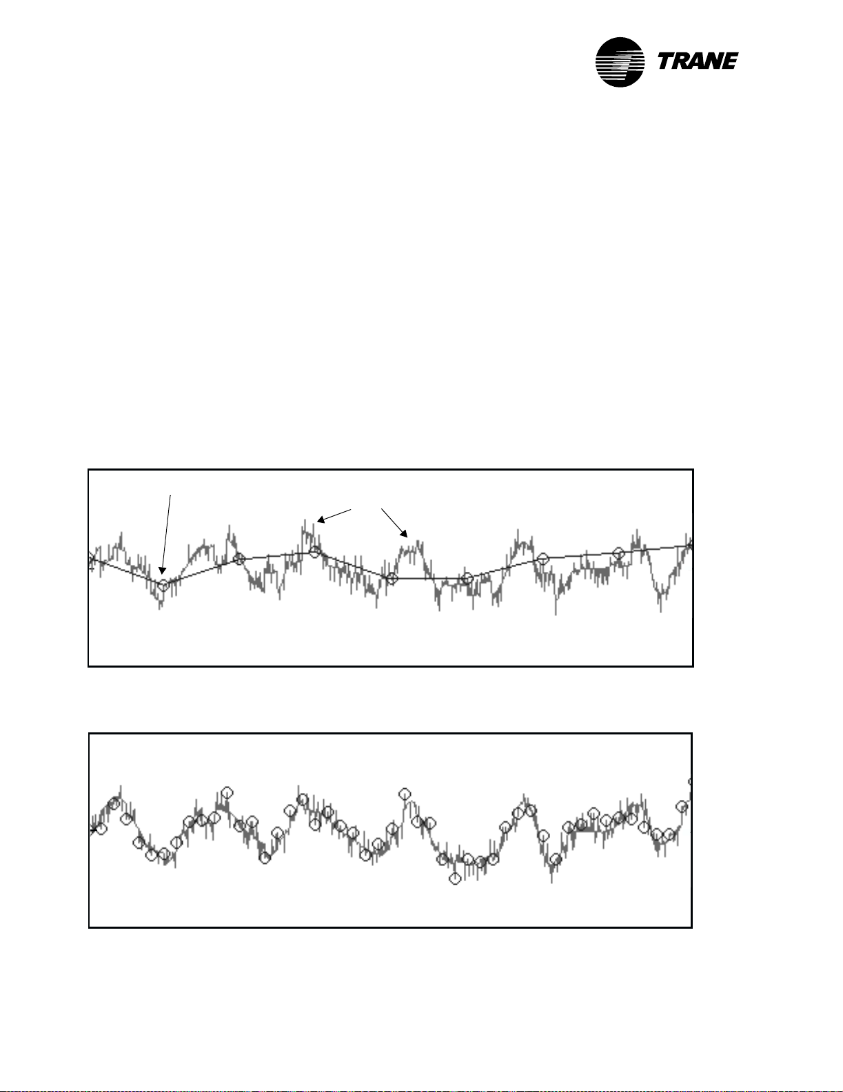
Figure 10 and Figure 11 show how aliasing can affect system response.
In Figure 10 the sampling frequency is too slow. Because of this, many of
the changes in duct static pressure are missed. In Figure 11 the sampling
frequency is fast enough that the changes in static pressure are tracked
accurately.
Sampling point
Duct static pressure
Figure 11: Sampling at the correct rate
Changes missed
by system
Time
Duct static pressure
Time
12 CNT-APG002-EN
Page 18
Sampling frequency
®
Problems also arise from sampling too quickly. Some systems have naturally slow response times, such as when measuring room temperature.
Slow response times can also be caused by equipment lags. Since PID
loops respond to error and changes in error over time, if the measured
variable changes slowly, then the error will remain constant for an
extended period of time. If the measured variable is sampled repeatedly
during this time, the proportional output remains about the same, but the
integral output becomes larger (since it is the sum of past errors). When
the control system does respond, the response is out of proportion to the
reality of the situation, which can destabilize the system. The control system should always wait to process the result of a change before making
another change.
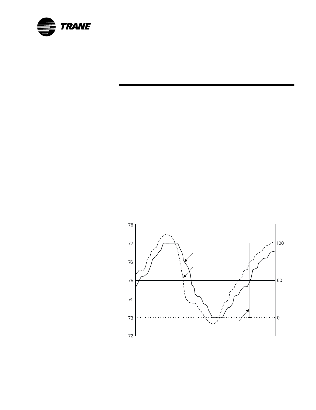
Figure 12 shows the measured variable when sampling frequencies are
too fast, acceptable, and barely acceptable. When the sampling frequency
is too fast (2 seconds), the measured variable begins to oscillate and
finally destabilizes because the PID loop output drives the actuator to
extremes. When the sampling frequency is slowed to either 10 or 20 seconds, the system remains stable once setpoint is reached.
Figure 12: System stability with different sampling frequencies
Sampling freq. = 10 s
Sampling freq. = 20 s
Sampling freq. = 2 s
(system destabilizes when
sampling freq. is too fast)
Measured variable
Time
CNT-APG002-EN 13
Page 19

®
Chapter 2 PID settings
Calculating the sampling frequency
PID loops are carried out by programs, such as process control language
(PCL) programs and Tracer graphical programming (TGP) programs.
Since the PID calculation occurs when the program executes, the sampling frequency and the program execution frequency are generally the
same.
Note:
Tracer controllers have different approaches to using the sampling frequency. For Tracer MP580/581 controllers, the sampling frequency can be a multiple of the program frequency. The
Tracer AH540 controller has a pre-determined sampling frequency. The Tracer MP501 controller has a setting for the sampling frequency.
Table 2 shows recommended program execution frequencies for common
applications. These are good initial values, but it may take some trial and
error to find the best frequency.
Table 2: Recommended initial sampling frequencies
Application Suggested execution frequency
Duct static pressure 5 seconds
Building static pressure 120 seconds
Discharge-air temperature 10 seconds
Space temperature (typical comfort zone) 60 seconds
Space temperature (high air change zone) 30 seconds
Duct humidity 10 seconds
Space humidity 30–60 seconds
You can also manually calculate the sampling frequency.
To calculate the sampling frequency:
1. Manually control the analog output to 0%.
For example, control a heating valve closed.
2. Record the measured variable when it stabilizes.
The temperature stabilizes at 70°F (21°C).
3. Manually control the analog output to 50% or 100%.
Control the output to 100% (completely opening the heating valve).
4. Record the measured variable when it stabilizes.
The temperature stabilizes at 120°F (49°C)
5. Subtract the measured variable determined in step 2 from the measured variable determined in step 4. This is the change in the measured variable.
120 – 70 = 50°F (49 – 21 = 28°C).
14 CNT-APG002-EN
Page 20

Calculating the sampling frequency
®
6. Calculate two-thirds (66%) of the change in measured variable determined in step 4. Add this value to the initial temperature to determine at what point two-thirds of the total change occurs.
In the example, 0.66 × 50°F = 33°F, so two thirds of the total change
occurs at 70°F + 33°F = 103°F (0.66 × 28°C = 18°C; 21 + 18 = 39°C).
7. Again, set the analog output to 0% and allow the measured variable
to stabilize.
The measured variable stabilizes at 70°F (21°C).
8. Control the output to the value used in step 3 and record the time it
takes to reach the two-thirds point determined in step 6. This is the
system time constant.
The time it takes to reach 103°F (39°C) is 2.5 minutes (150 seconds).
9. Divide the system time constant by 10 to determine the initial sampling frequency.
150 seconds ÷ 10 = 15 seconds.
Note:
The system time constant is the time it takes to reach 63.21% of
the difference between the start point and the end point. However, two-thirds (66%) is accurate enough for most purposes.
Figure 13 illustrates the procedure described above.
Figure 13: Determining the system time constant
Final value (valve open)
2/3 of total change
System time
Space temperature (°F)
constant
Initial value (valve closed)
Time (minutes)
CNT-APG002-EN 15
Page 21

®
Chapter 2 PID settings
Example
In this scenario, we want to find the sampling frequency for a PID loop
controlling a heating application.
1. Fully close the output.
2. The stabilized temperature is 60°F (16°C).
3. Fully open the output.
4. The stabilized temperature is 105°F (41°C).
5. The change in temperature is 105°F – 60°F = 45°F (41 – 16 = 25°C).
6. Two-thirds of the change in measured variable is 0.66 × 45°F = 30°F,
so two-thirds of the total change has occurred when the temperature
is 60°F + 30°F = 90°F (0.66 × 25°C = 17°C; 16 + 17 = 33°C).
7. Close the output. The temperature stabilizes.
8. Fully open the output. The time to reach 90°F (33°C) is 54 seconds (so
the system time constant is 54 seconds).
9. Divide the system time constant by ten, resulting in 54 ÷ 10 = 5.4.
The best initial sampling frequency is 5 seconds.
16 CNT-APG002-EN
Page 22

Action
®
Action
The action of a PID loop determines how it reacts to a change in the measured variable (such as a room temperature). A controller using direct
action increases the output when the measured variable increases. A controller using reverse action decreases the output when the measured variable increases.
Direct action
Figure 14 shows the temperature when a system is cooling a space. When
the error is large and the PID output is at 100%, the actuator and valve
combination are fully open. As the measured variable (room temperature)
decreases, the error becomes smaller, and the controller closes the valve
to reduce or stop cooling. Because the PID output and measured variable
move in the same direction (both decreasing), the loop is direct acting.
Figure 14: Cooling a space
Temperature
Measured variable
(temperature)
Error
Setpoint
Time
As temperature ↓
actuator position ↓
so action is direct
Reverse action
Figure 15 shows the temperature when a system is heating a space.
When the error is large and the PID output is at 100%, the actuator and
valve combination are fully open. When the measured variable (room
temperature) increases, reducing the error, the controller closes the valve
to reduce heating. Because the PID output and measured variable move
in opposite directions, the loop is reverse acting.
Figure 15: Heating a space
Time
Setpoint
Error
Te mp e ra tu r e
Measured variable
(temperature)
CNT-APG002-EN 17
As temperature ↑
actuator position ↓
so action is reverse
Page 23

®
Chapter 2 PID settings
Table 3: Action settings
Determining the action
Table 3 shows the action settings for several applications. These settings
are a good starting place for most applications.
Application Output
Discharge-air cooling Valve position 0–100% Completely open* Direct
Discharge-air heating Valve position 0–100% Completely open* Reverse
Duct static pressure Inlet guide vane position
0–100%
Duct static pressure variable-frequency drive
0–100%
Building static pressure Supply fan control Maximum fan speed Reverse
Building static pressure Exhaust fan control Maximum fan speed Direct
Discharge-air cooling Electric/pneumatic
5.0–15.0 psi (34–103 kPa)
Space temperature Discharge setpoint
50–100°F (10–37.8°C)
* These settings may vary by region
Actuator setting at 100%
PID output Direct or reverse acting
Completely open Reverse
Completely open Reverse
15.0 psi (103 kPa) Direct
N/A (calculates a setpoint) Reverse
To find the action for other applications, determine whether the actuator
and measured variable move in the same direction. If so, then the action
is direct. If not, then the PID loop is reverse acting.
Example 1
An exhaust fan controls the static pressure in a building. The exhaust fan
operates at its highest speed when the building pressure is too high.
When the pressure goes above the setpoint, the exhaust fan should speed
up to blow air from the building. So when the measured variable (the
building pressure) increases, the actuator increases the fan speed.
Because the measured variable and the actuator move in the same direction, the PID loop is direct acting.
Example 2
A supply fan controls the static pressure in ducts supplying variable-airvolume (VAV) boxes. The supply fan operates at its highest speed when
the pressure is too low. When the pressure goes above the setpoint, the
supply fan should slow down to blow less air to the VAV boxes. So when
the measured variable (the pressure) increases, the variable-frequency
drive (VFD) decreases the fan speed. Because the measured variable and
the control signal to the VFD move in opposite directions, the PID loop is
reverse acting.
18 CNT-APG002-EN
Page 24

®
Figure 16: Error deadband
Measured
variable
Error
Error deadband
Error deadband
Error deadband
Error deadband is typically used to minimize actuator activity. It can also
be used to allow for some slack in system sensors and actuator mechanics.
Error deadband prevents the PID output from changing when the absolute value of the error is less than the error deadband. For example, in
Figure 16 the error deadband is set at 2.0°F (1.1°C). As long as the absolute value of the error is less than the 2.0°F (1.1°C), the PID output cannot change. When the absolute value of the error exceeds 2.0°F(1.1°C),
the PID output can change.
control
Setpoint
control
Figure 16 illustrates the way that error deadband limits how often an
actuator is controlled. When a PID loop controls a chilled-water valve,
limiting control is not so important. But when a PID loop controls how
many stages of cooling are being used, it is important to limit equipment
cycling.
Typical applications
Table 4 shows reasonable error deadbands for several applications. The
error deadband can also be calculated as described in the following
sections.
Table 4: Error deadband settings
Application Suggested error deadband Notes
Modulating output
(analog or floating point binary)
Direct expansion
(DX) cooling
Cooling towers—
fan staging
0.5°F (0.3°C) for temperature
0.01 in. wc (2.5 Pa) for duct
static pressure
1.0 in. wc (250 Pa) for building static pressure
4.0°F (2.2°C) for temperature Staging application
2.5°F (1.4°C) for temperature Staging application
Dependent on resolution of the measuredvariable sensor
CNT-APG002-EN 19
Page 25

®
Chapter 2 PID settings
Adjusting error deadband for modulating outputs
In most applications, start with an error deadband of five or ten times the
sensor resolution. For example, thermistors have a resolution of approximately 0.1°F (0.06°C), so 0.5°F (0.3°C) is an appropriate error deadband.
This error deadband ensures that the sensor reading has changed an adequate amount before the controller responds.
IMPORTANT
The error deadband should not be smaller than the sensor resolution or
the controller will react to noise.
Adjusting error deadband for staged outputs
This section shows how to adjust the error deadband for staging applications. Refer to “Staging cooling-tower fans” on page 37 for information on
setting other PID properties for staging applications.
Finding the best error deadband for staged output applications is more
difficult than for modulating outputs. Instead of using a continuous actuator, such as a chilled-water valve, staged systems use binary outputs to
start and stop pieces of equipment, such as fans in a cooling tower. Each
piece of equipment contributes a set amount to the final output. When
determining the error deadband for staged outputs, the main goal is to
reduce equipment cycling.
Table 4 on page 19 provides useful initial values, but the error deadband
should be adjusted at the site with the equipment running.
Follow these guidelines when adjusting the error deadband:
• If possible, do not let equipment minimum-on and -off times control
how long a particular stage is used. Using minimum-on and -off times
to perform system control generally results in unpredictable behavior.
The error deadband should be set so that a stage is always on longer
than its minimum-on time.
• Ask how tight control should be. A smaller error deadband results in
tighter control, but control should not be so tight that minimum-on
and -off times affect the stages.
For example, for a variable-air-volume (VAV) air-handler turning on
cooling stages, control can be somewhat loose. The individual VAV
boxes control their valve to the space depending on the supply air
temperature. If the supply air temperature is relatively warm, the
VAV box allows more air flow. If the supply air temperature is somewhat cool, the VAV box constricts the air flow.
• The contribution of each stage can change depending on external cir-
cumstances, so make adjustments under worst case conditions.
Adjust the error deadband for cooling tower fan stages on very warm
days, and adjust the error deadband for boiler stages on very cold
days.
20 CNT-APG002-EN
Page 26

Other PID settings
®
With the preceding guidelines in mind, use the following procedure to
determine error deadband.
To adjust the error deadband for staged outputs:
1. Run the system manually.
If possible, do so under worst case conditions for the site. Although it
is not always possible for a technician to do this, it is possible for a
well-trained customer.
2. Find the smallest change in temperature, ∆T, that the first stage can
contribute (the quantity could also be building static pressure for fans
or flow for pumps).
Pay attention to possible changes in external circumstances, such as
the amount of water flow. If the system uses a lead-lag approach to
the equipment, it will be necessary to find the minimum ∆T for all
stages.
3. Multiply ∆T by 0.45 (the error deadband should be slightly less than
half of ∆T).
Keep in mind the resolution of the sensor. You may need to round the
error deadband to a more reasonable value.
4. Run the system with the new error deadband.
Each stage should be on longer than its minimum-on time and cycling
should be reduced as much as possible.
Other PID settings
Other PID settings not discussed in this chapter include:
• Proportional bias, which takes the place of derivative gain in propor-
tional-only control (see “Proportional calculation” on page 3)
• Minimum and maximum output, which limit the range of output of
the PID loop
• Enabled and disabled modes, which enable the PID output or disable
it to a default value
• Fail-safe mode, which sets the PID output to a default value if the
controller receives a fail flag from the hardware input that provides
the measured variable
Chapter 3, “Programming PID loops,” shows how to program these settings for Trane controllers.
CNT-APG002-EN 21
Page 27

®
Chapter 2 PID settings
22 CNT-APG002-EN
Page 28

®
Chapter 3
Programming PID loops
This chapter presents programs written in process control language
(PCL) and the Tracer graphical programming (TGP) editor. This chapter
does not discuss how to use the PCL or TGP editors. For information on
using these editors, refer to Universal Programmable Control Module
(UPCM) Programming Guide (EMTX-PG-5), Programmable Control Module (PCM) Edit Software Programming Guide (EMTX-PG-6), and Tracer
Graphical Programming applications guide (CNT-APG001-EN).
Programming in PCL
PID control is called direct digital control (DDC) in process control language (PCL). Table 5 shows how the DDC function is invoked in PCL. In
this example, DDC loop 4 compares the discharge-air temperature to the
heating discharge-air setpoint. Line 1 stores the result of the PID function in the analog variable HEATCALC. Line 2 controls the valve to the cal-
culated value. You can program specific PID settings in the DDC Loop
Parameters screen, shown in Table 6 on page 24.
Table 5: PID (DDC) loop in PCL
Line Result 1st Arg Operator 2nd Arg Description of Statement
---- -------- ----------- -------- ----------- ---------------------------------
1 HEATCALC = DISCHTMP DDC:4 HEATSP DDC loop 4 compares heat setpoint
to discharge-air temp
Result:
analog variable
2 HEATVLV = CONTROL HEATCALC Output controlled to HEATCALC
Measured variable:
analog input
analog variable
Loop name
Setpoint
analog input
analog variable
analog setpoint
analog parameter
:
value
CNT-APG002-EN 23
Page 29

®
Chapter 3 Programming PID loops
Table 6: PID settings in PCL
DDC LOOP # 4 HEAT VALVE
------------
PROPORTIONAL GAIN 4.00
INTEGRAL GAIN 1.00
DERIVATIVE GAIN 0.00
ACTION REVERS
PROPORTIONAL BIAS 0.0
MINIMUM OUTPUT VALUE 0.0
MAXIMUM OUTPUT VALUE 100.0
ERROR DIFFERENTIAL 0.5
Follow these steps to program PID loops in PCL:
1. Make sure that the setpoint is within reasonable limits.
Use the MIN and MAX operators to set a ceiling and floor for the setpoint, as shown in lines 1 and 2 of Table 7 on page 25.
2. Run the PID calculation and store the result in an analog variable.
Do not place the DDC operation in an IF clause (*IFT or *IFF)
because the output can be unpredictable.
3. Define failure and other operation-dependent conditions.
These checks are called the fail-safe and enable/disable functions.
Typically, check for fan status and measured variable input failures.
4. If the failure or enable/disable conditions from step 3 are met, set the
analog variable to some default value.
5. Control the analog output with the result of the calculation.
You can follow this procedure for most PID applications. All PID applications require failure-mode conditions.
Table 7 on page 25 shows a PCL program with enable/disable and failsafe logic. Line 4 checks whether the fan is on. Line 5 checks whether the
analog input has failed. Line 6 prevents the PID loop from being used if
the fan is off or the analog input has failed. If either condition is met, the
analog output is set to –10.0 (closed) in line 7. If the fan is on and the analog input has not failed, the PID loop controls the output in line 9.
24 CNT-APG002-EN
Page 30

Programming in PCL
®
Table 7: PCL program for PID loops
Line Result 1st Arg Operator 2nd Arg Description of Statement
---- -------- --------- -------- --------- ---------------------------------
1 CALC_SP = ROOM_SP MIN *80.0 Check that setpoint is reasonable
2 CALC_SP = CALC_SP MAX *65.0
3 PID_CALC = AIP1 DDC:1 CALC_SP Run PID calculation
4 *L1 = NOT FAN_ON Is the fan off? (Enable/disable)
5 *L2 = AIP1 FAIL Has the input failed? (Fail-safe)
6 *IFT = *L1 OR *L2 If fan is off or input has failed
7 PID_CALC = *-10.0 then set output to -10.0 (closed)
8*END =
9 AOP1 = CONTROL PID_CALC Control actuator to calculated value
Table 8 shows a PCL program with separated enable/disable and fail-safe
logic. The logic is separated because in this case the enable/disable and
fail-safe conditions have different results. In line 4, if the fan is off, then
the actuator is closed. In line 6, if the input sensor fails, then the actuator
is opened.
Table 8: Separate enable/disable and fail-safe logic
Line Result 1st Arg Operator 2nd Arg Description of Statement
---- -------- --------- -------- -------- -------------------------------------
1 CALC_SP = ROOM_SP MIN *80.0 Check that setpoint is reasonable
2 CALC_SP = CALC_SP MAX *65.0
3 PID_CALC = AIP1 DDC:1 CALC_SP Run PID calculation
4 *IFT = NOT FAN_ON If the fan off (Enable/disable)
5 PID_CALC = *-10.0 then set output to -10.0 (closed)
6 *IFT = AIP1 FAIL If the input has failed (Fail-safe)
7 PID_CALC = *100.0 then set output to 100.0 (fully open)
8 *END =
9 AOP1 = CONTROL PID_CALC Control actuator to calculated value
CNT-APG002-EN 25
Page 31

®
Chapter 3 Programming PID loops
Programming in TGP
Figure 17 shows the PID block used to program PID loops in TGP editor.
The PID block is more flexible than the DDC function in PCL. The enable/
disable and failure inputs can accept any binary value, regardless of
source. The setpoint, measured variable, p-gain, i-gain, and d-gain inputs
can accept any analog value, except analog outputs, including variable
(local or from a BAS), hardware input, and network input. You can program PID settings in the PID Properties dialog box, shown in Figure 18.
Figure 17: TGP PID block
Binary value
Output: analog value
Analog value
Figure 18: PID Properties dialog box
26 CNT-APG002-EN
Page 32

®
Figure 19: TGP program
Programming in TGP
Follow these steps to program PID loops in TGP:
1. Use the Limit block to make sure that the setpoint is within reasonable limits.
2. Run the PID calculation.
3. Define failure and other operation-dependent conditions.
Check for fan-status and measured-variable input failures. Program
sensible actuator positions or behavior for these conditions. To do
this, use the Default and Fail Safe fields in the PID Properties dialog
box (see Figure 18 on page 26), or use a Switch block for more complex
operations.
4. Control the analog output with the result of the calculation.
Figure 19 shows the TGP program for a simple PID loop controlling a
chilled-water valve. Compare the TGP program to the PCL program
shown in Table 7 on page 25. The Limit block accomplishes the same task
as the MIN and MAX operators in PCL.
Step 2. Run the PID calculation
Step 1. Limit setpoint to
a reasonable value
Step 3. Define failure and
enable/disable conditions
Step 4. Control the output
CNT-APG002-EN 27
Page 33

®
Chapter 3 Programming PID loops
28 CNT-APG002-EN
Page 34

®
Chapter 4
Applications
This chapter describes several HVAC applications that use PID control. It
includes specific settings and recommendations for each application.
Discharge-air temperature control
When controlling hot/chilled-water valves in discharge-air applications, a
PID loop controls the position of a valve to increase or decrease the flow of
hot or chilled water. This section focuses on control of hot-water valves,
but control of chilled-water valves is almost identical. Seasonal
changeover control may be required in these applications, but is not discussed here.
In this application, one hot-water valve and one chilled-water valve control the discharge-air temperature serving a large space. The hot-water
valve and chilled-water valve each require a PID loop. Since the two
valves should not be open simultaneously, the hot and chilled-water valve
programs share valve position data.
Table 9 shows a PCL program for controlling a hot-water valve. Note that
the variable CWVALVE provides the position of the chilled-water valve.
Table 9: PCL program to control a hot-water valve
Line Result 1st Arg Operator 2nd Arg Description of Statement
---- -------- --------- -------- -------- --------------------------------------
1 HEATCALC = DISCHTMP DDC:4 HEATSP HEATCALC is an analog variable that
holds result of PID calculation
2 *L0 = DISCHTMP FAIL Has discharge-air sensor failed?
3 *L1 = CWVALVE GT *0.0 Is chilled-water valve open?
4 *L2 = *L0 OR *L1
5 = FANOFF
6 *IFT = *L2 If sensor has failed, chilled-water
valve is open, or fan is off
7 HEATCALC = *-10.0 then close hot-water valve
8 *IFT = FANOFF AND HEATOPEN If fan is off and hot-water-valve-open
request (override) is true
9 HEATCALC = *100.0 then fully open hot-water valve
10 *END =
11 HWVALVE = CONTROL HEATCALC Control hot-water valve to calculated
position
12 *END =
CNT-APG002-EN 29
Page 35

®
Chapter 4 Applications
Figure 20 shows a TGP program to control a hot-water valve. Output Status 1 (an analog output) provides the position of the chilled-water valve. If
the chilled-water valve position is greater than zero, the hot-water valve
will not open.
Figure 20: TGP program to control a hot-water valve
Checks whether fan is off and
heat request is on
Checks whether fan is off or
chilled-water valve is open
If heat request is on and fan is
off, then output = 100, else
PID output controls actuator
Table 10 shows the initial values the technician used for the hot-water
valve PID loop. Chapter 2, “PID settings,” explains how to select initial
values for various PID applications.
Ta b l e 10 : Hot-water valve control settings
PID setting Initial value Final value
Proportional gain 2.0 4.0
Integral gain 0.5 1.0
Derivative gain 0.0 0.0
Proportional bias 0.0 (not used in PID mode) 0.0
Error deadband 0.5 0.5
Action Reverse Reverse
Sampling frequency 10 seconds 30 seconds
30 CNT-APG002-EN
Page 36

Discharge-air temperature control
®
After the initial installation and testing, the technician noticed that the
discharge-air temperature was oscillating in a 10°F (5.6°C) band around
setpoint. Slowing the sampling frequency to 30 seconds stopped the oscillations (see Chapter 5, “Troubleshooting”). The technician also increased
the proportional and integral gains to make the discharge-air temperature reach setpoint faster.
Figure 21 shows the discharge-air temperature and valve position over a
two-hour period. During the unoccupied period, the hot-water valve is
completely open. Eventually the discharge-air temperature rises to
almost 100°F (37.8°C). At the twelve-minute point, the HVAC system
changes from the unoccupied to the occupied state, and the hot-water
valve is adjusted to meet the discharge-air setpoint. The valve closes completely for nearly 20 minutes until the discharge-air temperature drops
below setpoint. Achieving a stable discharge-air temperature takes
approximately 30 minutes. Note that once setpoint is reached, the valve
position remains stable between 10% and 15%. A stable valve position
over time indicates that the loop has been tuned for optimal performance.
Figure 21: Hot-water valve position and discharge-air temperature
Discharge-air
temperature (°F)
DA Temperature and valve position
Discharge-air temperature
setpoint (°F)
Heat valve position during
change from unoccupied
to occupied state
Valve position (%)
Time (minutes)
CNT-APG002-EN 31
Page 37

®
Chapter 4 Applications
Building pressure control
Space pressure is typically controlled by opening and closing relief dampers. A PID loop controls these dampers based on a space pressure setpoint
and the measured space pressure. The space pressure in the building
should remain slightly positive to keep dust particles out, but not so positive that outside doors are difficult to open.
Table 11 shows a PCL program to control a relief damper. Figure 22
shows the same program in TGP. In PCL, the space pressure and other
values are scaled by a factor of 100 because the software resolution is 0.1
and the sensor resolution is 0.01. Values are not scaled in TGP.
Ta b l e 11 : PCL program for relief damper control
Line Result 1st Arg Operator 2nd Arg Description of Statement
---- -------- --------- -------- -------- --------------------------------------
1 PRSPX100 = SPACEPR * *100.0 Scale the measured space pressure
2 RELCALC = PRSPX100 DDC:2 SPACPRSP Call the PID (or DDC) function
3 *L0 = SPACEPR FAIL Has pressure sensor failed?
4 *IFT = *L0 OR FANOFF If sensor has failed or fan is off
5 RELCALC = *-10.0 then set output to -10 to close valve
6 *END =
7 RELDAMPR = CONTROL RELCALC Control damper to calculated position
8 *END =
Figure 22: TGP program for relief damper control
32 CNT-APG002-EN
Page 38

Building pressure control
®
Table 12 lists the settings for the PID loop controlling building pressure.
The sampling frequency is slow because building pressure changes slowly.
For programs written in PCL, the error deadband is 1.0, which is equal to
100 times the minimum resolution of the pressure sensor.
Table 12: Settings for building pressure control
PID setting Initial value
Proportional gain 4.0
Integral gain 1.0
Derivative gain 0.0
Error deadband PCL: 1.0, TGP: 0.01
Action Direct
Sampling frequency 2 minutes
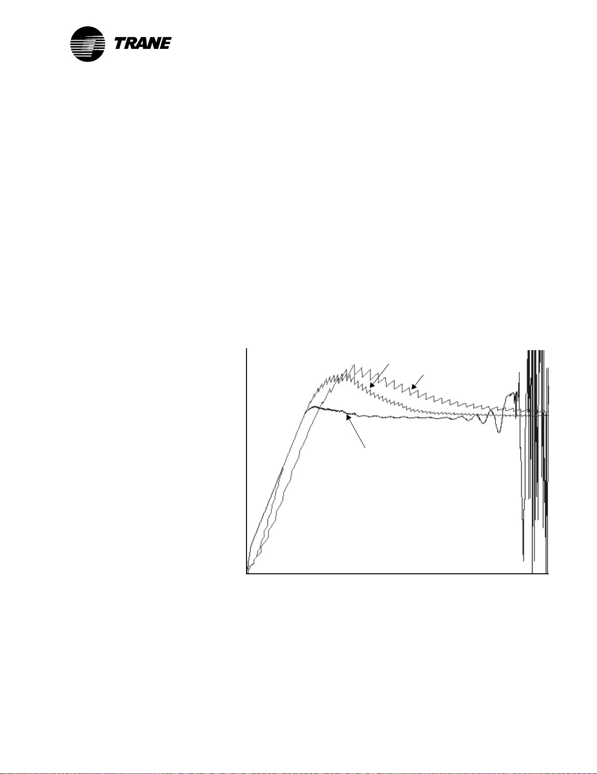
Figure 23 shows system response over a 14-hour period. During the unoccupied period (from 150 to 650 minutes) a different type of control, which
decreases pressure, is being used. After the control mode changes from
occupied to unoccupied, the PID loop still attempts to increase space pressure by closing the relief damper.
When the space is again occupied, the rapid change in the damper position indicates that the system is being aggressively controlled.
You may find that during occupied operation, the relief damper is controlled to a fully open position. This is usually the result of pressure in an
adjacent space influencing pressure in the measured space.
Figure 23: Space pressure and damper position
Relief damper
position (%)
Unoccupied
100 × space pressure
Space pressure and valve position
setpoint (in. wc)
100 × space pressure
(in. wc)
Time (minutes)
CNT-APG002-EN 33
Page 39

®
Chapter 4 Applications
Cascade control—first stage
A PID loop can be used to automatically determine a discharge-air temperature setpoint. Other programs or control systems can then make use
of this calculated setpoint. This type of control, called cascade control,
results in very tight control of space temperature. Calculating the discharge-air temperature setpoint is the first stage of cascade control.
Figure 24 illustrates how a PID loop calculates the discharge-air temperature setpoint. The calculated discharge-air temperature is changed
based on the difference between the space temperature setpoint and the
space temperature.
Figure 24: Calculating the discharge-air temperature setpoint
Space
setpoint
+
Error
Σ
–
Space
temperature
PID calculation
Discharge-air
temperature setpoint
Cascade control requires two sensors, one for the space temperature and
one for the discharge-air temperature. The PCL or TGP program must be
programmed to respond to a failure of either of the sensors. Suggested
failure conditions are:
• If the space temperature sensor fails, set the discharge-air tempera-
ture setpoint to the space temperature setpoint. Other limits for the
discharge-air temperature setpoint may need to be defined. Inform
the operator of the sensor failure.
• If the discharge-air temperature sensor fails, control the hot or
chilled-water valve as appropriate to the climate in your region.
Inform the operator of the sensor failure.
Table 13 shows a PCL program to calculate the discharge-air temperature setpoint, and Figure 25 on page 35 shows the same program in TGP.
Most of the programming occurs in the DDC Loop Parameters screen. Use
the values shown in Table 14 on page 35.
Table 13: PCL program for discharge-air temperature setpoint in cascade control
Line Result 1st Arg Operator 2nd Arg Description of Statement
---- -------- --------- -------- -------- --------------------------------------
1 DATSTPT = SP_TEMP DDC:1 SP_STPT Call the PID function
2 *IFT = SP_TEMP FAIL If the space sensor has failed
3 DATSTPT = SP_STPT set the disch air setpt to space setpt
4 *END = (Note: the discharge-air temp sensor is
checked in another program.)
34 CNT-APG002-EN
Page 40

Cascade control—first stage
®
Figure 25: TGP program for discharge-air temperature setpoint in cascade control
If space temperature sensor has
failed, switch control to space
temperature setpoint
If you use the settings shown in Table 14, you should not have to tune the
loop. These values can be used in almost any cascade control application
without change. The proportional and integral gains are high to respond
aggressively to the error and change in error. The minimum and maximum output values keep the output between 50°F (10°C) and
120°F(49°C).
Table 14: Settings for discharge-air temperature setpoint
PID setting Initial value
Proportional gain 20.0
Integral gain 5.0
Derivative gain 0.0
Error deadband 0.5
Action Reverse
Sampling frequency 60 seconds
Minimum output 50°F
Maximum output 120°F
Figure 26 on page 36 shows an example of the relationship between the
calculated discharge-air temperature setpoint and the space temperature.
The discharge-air temperature setpoint reacts strongly to small changes
in error because of the high proportional gain.
CNT-APG002-EN 35
Page 41

®
Chapter 4 Applications
Figure 26: Space temperature and calculated discharge-air setpoint
PID calculated
discharge-air setpoint
Space temperature
Space setpoint
Temperature (°F)
Time (minutes)
The discharge-air temperature setpoint calculated by the PID loop may
not control the discharge-air temperature depending on other conditions
that have priority, such as high and low setpoint limits. The high limit
controls the discharge-air temperature for much of the time in Figure 27
(because the calculated setpoint is too high). Also, Figure 27 shows how
aggressively the PID loop responds to disturbances in space temperature.
Figure 27: Effective discharge-air temperature setpoint
Space temperature
Space setpoint
PID calculated
discharge-air setpoint
Effective discharge-air
temperature setpoint
Temperature (°F)
Time (minutes)
36 CNT-APG002-EN
Page 42

Staging cooling-tower fans
®
Staging cooling-tower fans
Staging applications organize individual pieces of equipment into a group
to accomplish a single task. For example, several fans might be used to
maintain the supply water temperature in a cooling tower. Staging applications control a series of binary outputs on and off at specific times based
on an analog value. This value can be generated by a linear equation, a
PID calculation, a reset block, and so on.
The advantage of using PID control for staging applications is that you
can use the error deadband to optimize the system so that stages cycle
less often (see “Adjusting error deadband for staged outputs” on page 20).
Another advantage is that PID control is built into Trane controllers,
making settings easy to enter and adjust.
This section describes how to use a proportional-only PID loop to control
supply water temperature in a cooling tower with several fans instead of
a variable-frequency drive.
Setting up the PID loop
Proportional-only control works well in staging applications because the
output is linear and predictable, and therefore easy to manage. Integral
control can also be used but is much more complex to set up and tune.
To use proportional-only control in process control language (PCL), set
the integral and derivative gains to zero. In Tracer graphical programming (TGP) editor, select Proportional Only in the PID Properties dialog
box (see “Programming in TGP” on page 26).
CNT-APG002-EN 37
Page 43

®
Chapter 4 Applications
The PCL program in Table 15 stages two cooling-tower fans. Figure 28
shows the same program in TGP. The behavior of the stages programmed
in this program is illustrated in Figure 30 on page 41.
Table 15: PCL program for staging cooling-tower fans
Line Result 1st Arg Operator 2nd Arg Description of Statement
---- -------- --------- -------- -------- --------------------------------------
1 FAN_CALC = CWST DDC:1 CW_SETP DDC loop compares water temp to setpt
2 *IFF = CDWP1ST OR CDWP2ST If both chilled-water pumps are off
3 FAN_CALC = *0.0 set output to 0 to turn off all fans
4 *IFT = CWST FAIL If sensor has failed
5 FAN_CALC = *100.0 set output to 100 to turn on all fans
6 *IFT = FAN_CALC GT *63.0 If PID result > 63
7 CT1SS = CONTROL ON then turn on stage 1
8 *IFT = FAN_CALC LT *10.0 If PID result < 10
9 CT1SS = CONTROL OFF then turn off stage 1
10 *IFT = FAN_CALC GT *90.0 If PID result > 90
11 CT2SS = CONTROL ON then turn on stage 2
12 *IFT = FAN_CALC LT *36.0 If PID result < 36
13 CT2SS = CONTROL OFF then turn off stage 2
14 *END
Figure 28: TGP program for staging cooling tower fans
Integral and derivative gains need
values even though the PID block
is set to proportional only
Deadband blocks set
on/off points for each fan
38 CNT-APG002-EN
Page 44

Staging cooling-tower fans
®
The TGP program follows this sequence of operation:
1. Chilled-water pump status is checked. If there is flow, the cooling
towers are allowed to operate.
2. Based on the error (the difference between the chilled-water setpoint
and the chilled-water temperature), the controller turns cooling-tower
fans on or off as needed to ensure efficient cooling tower operation.
3. If the chilled-water temperature sensor fails, all cooling-tower fans
are turned on.
Note that:
• A 2-input Or block (a TGP block) checks the status of the chilled-
water pumps. Both fan stages are turned off if neither chilled-water
pump is operating.
• A PID calculation generates an output based on the difference
between the chilled-water setpoint and the chilled-water temperature. If both pumps are off, the PID calculation is disabled and the
output set to the default of zero.
• If the chilled-water temperature sensor fails, the PID output defaults
to the fail-safe value of 100, which turns both fan stages on.
Specific settings are listed in Table 16.
Table 16: Settings for staging cooling-tower fans
PID setting Initial value
Proportional gain 17 (midrange between 10 and 26)
Integral gain 0
Derivative gain 0
Proportional bias 63% (set the same as the first stage enable value)
Error deadband 2.0°F (1.1°C)
Action Direct
Sampling frequency At least 1 minute
The throttling range is fairly wide—from 10°F to 25°F (6°C to 14°C). The
large throttling range keeps control loose to prevent stages from cycling
too often. Assuming an output range from 0 to 100, the throttling range
translates to a proportional gain of 26 to 10 respectively (see “Calculating
the gains” on page 11). The proportional gain chosen for this application
is in the middle of that range at 17. The gain may need to be adjusted to
optimize the system.
The temperature of the water flowing through a cooling tower responds
fairly slowly, so the sampling frequency should be set to at least 1 minute.
The sampling frequency may need to be adjusted to a slower rate if the
temperature oscillates around the setpoint (see “Calculating the sampling
frequency” on page 14). The goal in this case is to effectively control the
water temperature while limiting equipment cycling.
CNT-APG002-EN 39
Page 45

®
Chapter 4 Applications
The challenge in staging applications is to find the correct proportional
bias. This value determines the output when the error is zero. The proportional bias should have the same value as the point at which the first
stage turns on (see “Determining the staging points” on page 42). In this
case, the first stage turns on at an output of 63%, so the proportional bias
is set to 63%.
Figure 29 shows the output versus error when the proportional bias is
63%. This graph can help us determine the error deadband setting. We
know that the first-stage fan turns on when the error becomes negative.
The second stage should not turn on until the output reaches 90% or an
error of –4°F (–2.2°C). Following the procedure presented in “Adjusting
error deadband for staged outputs” on page 20, the error deadband is:
0.45 × 4°F (2.2°C) = 1.8°F (1°C)
We can round the error deadband to 2.0°F or 1.5°F. Either choice should
ensure that the second stage does not turn on until the error is relatively
large.
Figure 29: Controller output versus error: proportional bias = 63%
Controller output (%)
90% point
Proportional bias = 63%
10% point
Error
40 CNT-APG002-EN
Page 46

Staging cooling-tower fans
®
For staging applications, the result of the PID calculation controls binary
outputs rather than an analog output. For this kind of staging application, it is typical to use the deadband to make sure that the binary output
state is maintained for some specific range. Figure 30 illustrates the staging points for two cooling-tower fans. The three lines indicate (from bottom to top): the number of fans versus the control value, fan 1 on and off
points, and fan 2 on and off points. Fan 1 is turned on at 63% and off at
10%. Fan 2 is turned on at 90% and off at 36%.
Figure 30: Cooling tower fan on and off points
Fan 2
Fan 1
2
No. of
1
fans
0
0 10 20 30 40 50 60 70 80 90 100
Control value (%)
CNT-APG002-EN 41
Page 47

®
Chapter 4 Applications
Determining the staging points
This section describes how to find the points at which stages are turned
on and off.
Start with these guidelines:
• To avoid having a stage turn off at the lowest extreme, always have at
least one stage on at 10% of the output range. Turn that stage off
when the control value is less than 10%. Due to hysteresis (the programming of equipment to react in a different way depending on
whether the control value is increasing or decreasing), this stage may
be on only when the output is decreasing.
• To avoid having a stage turn on at the PID maximum value, have all
stages on at 90% of the output range.
• To reduce equipment cycling, stages should overlap.
• As a starting point, assume that the overlap range is the same for all
stages. You can adjust the staging points later to optimize the system.
To determine the staging points:
1. Use the following formula to find the overlap range:
Overlap range
Overlap range
(assuming the system has three fans).
2. To create overlap, the first stage should turn on at the lowest extreme
plus 2 times the overlap range and turn off at the lowest extreme, or:
Stage 1
For a three-fan system, the first stage should turn on at 50% and turn
off at less than 10%.
3. For each subsequent stage, the on and off points are described by:
Stage n
Although not discussed in this section, equipment minimum-on and -off
times become a factor as more stages are added to the system. The higher
stages may be on for shorter periods of time. System behavior may
become erratic if a stage control is dominated by minimum-on and -off
times instead of the calculated control value.
=
=
highest extreme lowest extreme–
--------------------------------------------------------------------------------------------=
90% 10%–
----------------------------------------stage count 1+
On: control value 10% 2 overlap range×()+50%=≥
Off: control value 10%<
On: control value 10% n 1+()overlap range×+≥
Off: control value 10% n 1–()overlap range×+<
stage count 1+
80%
-------------20%===
31+
42 CNT-APG002-EN
Page 48

®
Example 1: Two-stage fan system
The staging points are calculated as follows:
1. Calculate the overlap range.
Staging cooling-tower fans
Overlap range
80%
----------------------------------------stage count 1+
80%
-------------26.7%===
21+
2. Calculate the first stage control points.
Stage 1
On: control value 10% 2 26.7× %()+63%≈≥
=
Off: control value 10%<
3. Calculate the second stage control points.
On: control value 10% 3 26.7× %()+90%=≥
Stage 2
=
Off: control value 10% 1 26.7× %()+36%≈<
The staging points are illustrated in Figure 31. You should not have to
adjust the extremes at 10% and 90%, but you may need to adjust the middle staging points to optimize the system.
Figure 31: Two-stage fan on and off points
Fan 2
Fan 1
2
No. of
1
fans
0
0 10 20 30 40 50 60 70 80 90 100
Control value (%)
CNT-APG002-EN 43
Page 49

®
Chapter 4 Applications
Example 2: Three-stage fan system
The staging points are calculated as follows:
1. Calculate the overlap range.
Overlap range
80%
----------------------------------------stage count 1+
80%
-------------20%===
31+
2. Calculate the first stage control points.
Stage 1
On: control value 10% 2 20× %()+50%=≥
=
Off: control value 10%<
3. Calculate the second stage control points.
On: control value 10% 3 20× %()+70%=≥
Stage 2
=
Off: control value 10% 1 20× %()+30%=<
4. Calculate the third stage control points.
On: control value 10% 4 20× %()+90%=≥
Stage 3
=
Off: control value 10% 2 20× %()+50%=<
The results are summarized in Figure 32.
Figure 32: Three-stage fan on and off points
Fan 3
Fan 2
Fan 1
3
No. of
fans
44 CNT-APG002-EN
2
1
0
0 10 20 30 40 50 60 70 80 90 100
Control value (%)
Page 50

®
Chapter 5
Troubleshooting
This chapter offers a general troubleshooting procedure and tips for specific problems.
Troubleshooting procedure
When following this troubleshooting procedure, change only one thing at
a time, then wait to see the effect the change has on the system.
Follow these steps to troubleshoot a PID loop:
1. Make sure that the system is not in override.
2. Graph the measured variable, setpoint, and valve position over time
to determine how the system performs.
Look at the big picture. Can the system actually accomplish what it
needs to? What is happening to the measured variable? Is it oscillating or failing to reach setpoint?
3. Check the programming logic for:
• DDC statement in an *IFT or *IFF clause
• Failure conditions that are always true
• Output connected to the wrong part of a Switch block in TGP
• Conflicting programming demands, such as bad logic interlocks
between program modules
4. Check PID property settings for:
• Output minimum incorrectly set to 100%
• Output maximum incorrectly set to 0%
• Sampling frequency that is too fast
5. Check the system for disturbances from:
• Outside air intake
• Bad actuator linkages
• Faulty sensors
6. Change PID gains.
• Reduce gains when experiencing system overshoot, output at
minimum or maximum, or cycling of output around setpoint
• Increase gains when experiencing system undershoot
CNT-APG002-EN 45
Page 51

®
Chapter 5 Troubleshooting
Tips for specific problems
Table 17 provides tips for troubleshooting specific problems.
Ta b l e 17 : Tips for specific problems
Problem Tips
Measured variable is
cycling around setpoint
Overshooting setpoint Reduce gains
Undershooting setpoint Increase gains
Output at maximum Ensure that minimum output is not set to 100%
Output at minimum Ensure that maximum output is not set to 0%
Changing the sampling frequency
The major cause of actuator cycling is time lags in the system. If a 10%
change in PID output requires two minutes to affect the measured variable, it does no good to have the sampling frequency set to two seconds.
The integral contribution will build up before any significant change in
error can be measured. A sampling frequency of 30 to 60 seconds would
work much better in this situation. In other words, to fix a cycling system,
slow down the loop. See “Sampling frequency” on page 12 for more infor-
mation.
• Slow the sampling frequency
• Decrease PID gains
• Check programming for conflicting actuator
commands
• Actuators may be overridden by minimum-on
and -off times
Changing the gains
Be careful when changing PID gains. Never change the gains unless the
effects can be measured. Use a doubling/halving technique when increasing or decreasing gains. If the PID gains are set to 4, 1, and 0 respectively,
and you are going to reduce them, try 2, 0.5, and 0. If the system now
undershoots, try gains of 3, 0.75, and 0 respectively. Refer to “Throttling
range” on page 9 for more information.
46 CNT-APG002-EN
Page 52

Examples
®
Examples
This section presents troubleshooting scenarios from a hot-water valve
application. The three examples have the same symptom but different
solutions to the problem.
Example 1
A hot-water valve cycles closed every few minutes. Although the space
temperature remains fairly stable, the discharge-air temperature swings
across a range of 10°F (5.6°C).
The technician follows the troubleshooting procedure described in this
chapter. However, nothing seems to work. The program is the same as the
one used in “Discharge-air temperature control” on page 29, and is known
to work well. Reducing the sampling frequency reduces the cycling, but
does not eliminate it. Reducing the gains helps reduce the cycling further,
but now the discharge-air temperature takes too long to reach setpoint.
The valve continues to cycle closed, though not as often.
The technician goes back through the troubleshooting steps and notices
when checking the programming logic that the hot-water valve closes
when the chilled-water valve is open. The technician decides to check the
position of the chilled-water valve while the application is running with
its original settings. Figure 33 illustrates what the technician found. The
chilled-water valve opens when the discharge-air temperature goes above
setpoint, thus forcing the hot-water valve to close.
Figure 33: Hot and chilled-water valve positions
Discharge-air
temperature setpoint (°F)
Hot-water valve
position (%)
Discharge-air temperature and valve position
Time (minutes)
Discharge-air
temperature (°F)
Chilled-water valve
position (%)
CNT-APG002-EN 47
Page 53

®
Chapter 5 Troubleshooting
The application is running in a cold climate during winter, so the chilledwater valve should not open at all (because chilled water is not being
used). However, it might open in the following cases:
• The building automation system has information that chilled water is
available.
• The program logic is wrong, and the hot-water valve should depend
only on the heat/cool mode, not on the position of the chilled-water
valve.
Before reprogramming the controller, the technician checks to see if the
building automation system has information that chilled water is available. The technician finds that the building automation system had been
configured incorrectly and is sending the controller information that
chilled water was available. To fix the problem, the technician resets the
building automation data point. The controller no longer opens the
chilled-water valve, which in turn prevents the hot-water valve from
cycling closed every few minutes.
Example 2
The technician experiences the same problem as in the first example: a
hot-water valve cycles closed every few minutes, and the discharge-air
temperature swings across a range of 10°F (5.6°C).
Again, the technician follows the troubleshooting procedure. The programming logic looks correct. The mixed air temperature and outdoor air
temperature remain steady, indicating that outside disturbances are not
causing the problem. The cycling stops only when the technician slows
the sampling frequency from 10 seconds to 30 seconds.
When the sampling frequency is 10 seconds, the hot-water valve cycles
because the fast sampling frequency does not take into account the natural lag involved in trying to change air temperature. The change in the
discharge-air temperature over 10 seconds is so small that the controller
responds more aggressively to reduce the error. The controller opens the
hot-water valve too much, which causes the discharge-air temperature to
overshoot the setpoint (see Figure 34 on page 49). Again, the controller
over-reacts, shutting the hot-water valve to cool the discharge-air temperature, which causes the discharge-air temperature to overshoot the setpoint in the opposite direction. This cycle repeats indefinitely.
Slowing the sampling frequency to 30 seconds gives the discharge-air
temperature enough time to change so that the PID loop can calculate the
valve position based on a reasonable error.
48 CNT-APG002-EN
Page 54

Examples
®
Figure 34: Hot-water valve position, sampling frequency too short
Discharge-air temperature and valve position
Discharge-air
temperature setpoint (°F)
Hot-water valve
position (%)
Time (minutes)
Discharge-air
temperature (°F)
CNT-APG002-EN 49
Page 55

®
Chapter 5 Troubleshooting
Example 3
The technician experiences the same problem as in the first two examples: a hot-water valve cycles closed every few minutes, and the discharge-air temperature swings across a range of 10°F (5.6°C). The
technician graphs the discharge-air temperature setpoint and the hotwater valve position, as shown in Figure 35.
Figure 35: Hot-water valve position, gains too high
Discharge-air
temperature setpoint (°F)
Hot-water valve
position (%)
Discharge-air temperature and valve position
Time (minutes)
Discharge-air
temperature (°F)
The dramatic changes in the hot-water valve position indicate that the
gains are too high. The technician reduces the proportional gain from 16
to 1 and the integral gain from 4 to 0.25. This stops the hot-water valve
from cycling but increases the time to reach setpoint to more than 20 minutes. The technician then increases the proportional gain to 4 and the
integral gain to 1, which brings the discharge-air temperature to setpoint
more quickly while still preventing the hot-water valve from cycling.
50 CNT-APG002-EN
Page 56

®
Chapter 6
Frequently asked questions
Why is the output of my PID loop always zero?
•
Maximum PID output may be set to zero.
• PID action setting may need to be changed.
• Setpoint may be zero or negative, driving the output to zero. Change
the setpoint to a reasonable value manually or add a limit block to the
PID loop to keep the setpoint within a reasonable range.
• Physical output may not have enough power to achieve the setpoint,
leaving the output at the low end of its range. This problem is known
as integral windup (see “Integral calculation” on page 4 for more
information).
• Measured-variable input may have failed and the fail-safe may be set
to zero.
• Fan status is off so the program has set the output to zero.
• Scaling may be inconsistent for setpoints and inputs.
Why is the output of my PID loop always at its maximum value?
•
Minimum PID output may be set to the maximum value.
• PID action setting may need to be changed.
• Setpoint may be high enough that the output stays at its maximum
output. Change the setpoint to a reasonable value or add a limit block
to the PID loop to keep the setpoint within a reasonable range.
• Physical output may not have enough power to achieve the setpoint,
leaving the output at the high end of its range. This problem is known
as integral windup (see “Integral calculation” on page 4 for more
information).
• Measured-variable input may have failed and the fail-safe may be set
to the maximum value.
• Scaling may be inconsistent for setpoints and inputs.
Why is the output of my PID loop oscillating?
•
PID action setting may be wrong. If the action is reverse when it
should be direct, the system may start oscillating as the output
changes around setpoint.
• Sampling frequency may be too slow or too fast. See “Sampling fre-
quency” on page 12 for instructions on setting an appropriate sampling frequency.
• Proportional, integral, or derivative gains may be set too high. Reduce
the gains until the oscillation subsides.
CNT-APG002-EN 51
Page 57

®
Chapter 6 Frequently asked questions
I tried the 4:1 ratio for proportional and integral gains, but this
did not optimize my system. Can I try another ratio?
We recommend maintaining a 4:1 ratio between the proportional and
integral gains. Changing the gains may slightly improve the speed and
stability of a system, but the 4:1 ratio has proven to work effectively. See
“Calculating the gains” on page 11 for more information.
Why is the derivative gain usually zero?
Derivative control is rarely used in HVAC applications because the large
error deadbands used in HVAC applications make derivative control ineffective. Also, derivative control can react to noise in the input signal, and
the lag in derivative control makes tuning difficult. Setting the derivative
gain to zero prevents derivative control from being used. See “Derivative
calculation” on page 5 for more information.
What is the difference between direct acting and reverse acting?
Reverse acting loops decrease the output as the measured variable
increases. Discharge-air heating, duct static pressure control, and space
temperature control applications are typically reverse acting. Direct acting PID loops increase the output as the measured variable increases.
Discharge-air cooling and building static pressure (with exhaust fans)
applications are typically direct acting. See “Action” on page 17 for more
information.
When should I use proportional-only control?
Proportional-only control works well in staging applications because it
can be simpler to manage than full PID control. Proportional-only control
is also used in pneumatic controllers. To use proportional-only control, set
the integral and derivative gains to zero. See “Proportional calculation”
on page 3 for more information.
Why should I use PID control in staging applications?
Most Trane controllers have built-in PID functions, making settings easy
to enter and adjust. See “Staging cooling-tower fans” on page 37 for more
information.
How can I tell if a PID loop is working well?
Graph the measured variable, setpoint, and valve position over time,
especially during periods of change, such as when changing from unoccupied to occupied mode. The setpoint should be achieved in a reasonable
time and the valve position should remain fairly stable once setpoint has
been reached. If the measured variable oscillates around the setpoint,
fails to reach setpoint, or takes too long to reach setpoint, follow the
guidelines in Chapter 5, “Troubleshooting.”
52 CNT-APG002-EN
Page 58

Frequently asked questions
®
What’s the best sampling frequency?
The best sampling frequency depends on the application. See “Calculat-
ing the sampling frequency” on page 14 for recommended sampling frequencies. You may need to adjust the sampling frequency (usually to slow
it down). If the measured variable is oscillating around setpoint, the sampling frequency may be too fast or the gains may be too big.
Do I need to worry about the throttling range?
You probably do not need to worry about the throttling range. The throttling range cannot be programmed as a PID setting. Instead, it is used to
help calculate the gains. The throttling range is the amount of error it
takes to move the output of a system from its minimum to its maximum
setting. Most PID applications have recommended gain settings, but if
these gains do not fit your application, an understanding of throttling
range can help you find more appropriate gain settings. See “Throttling
range” on page 9 and “Calculating the gains” on page 11 for more
information.
CNT-APG002-EN 53
Page 59

®
Chapter 6 Frequently asked questions
54 CNT-APG002-EN
Page 60

®
Appendix A
The math behind PID loops
This appendix presents the mathematical formulas used for PID control
in Tracer MP580/581 controllers, the programmable control module
(PCM), and the universal programmable control module (UPCM).
Velocity model formula
The formula used to calculate the output in the velocity model is shown
below. It uses the integral and proportional gain, but not the derivative
gain. The same formula is used in the PCM and the UPCM.
K
prop
∆output n()
Where:
K
= proportional gain
prop
K
= integral gain
int
= integral gain
K
diff
c = 2.56 for the PCM and UPCM
c = 1.00 for Tracer MP580/581 controllers
∆error n()
∆2error n()
The factor 2.56 scales the PID output to a range of 0–100% in the PCM
and UPCM.
--------------
= change in error
= change in the change squared
∆error n()×
c
error n()×
K
int
-----------------------------------------
c
K
diff
------------
c
2
∆
error n()×++=
Proportional control formula
The following formula shows the relationship between the error and the
output in proportional-only control:
K
prop
Output n()
--------------
error n()× proportional bias+=
c
The proportional bias calibrates the controller to some known output. So
when the error is zero (which makes the proportional gain zero), the output is equal to the proportional bias.
CNT-APG002-EN 55
Page 61

®
Appendix A The math behind PID loops
56 CNT-APG002-EN
Page 62

®
Glossary
action
A PID setting that determines how the PID loop reacts to a change in the
measured variable (such as a room temperature). A controller using
direct action increases the output when the measured variable increases.
A controller using reverse action decreases the output when the measured variable increases. See also measured variable.
actuator
Electric, hydraulic, or pneumatic motor that changes the position of
moveable devices such as valves and dampers.
cascade control
A method of control in which one PID loop calculates a setpoint for use by
other PID loops or control systems. Cascade control is used in applications that require tight control; the response to error is aggressive.
conversion function
The part of a PID loop that converts the measured variable to the same
units of measurement as the setpoint. The result of the conversion function is called the measured variable or process variable.
deadband
See error deadband.
derivative control
Control action based on the rate of change of the error. Used to smooth an
actuator motion or cause an actuator to react faster. Derivative control is
rarely used in HVAC applications.
direct action
See action.
direct digital control (DDC)
A term used at Trane as a synonym for PID control.
error
In PID control, the difference between the setpoint and the measured
variable. For example, if the setpoint is 75°F (23.9°C) and the measured
variable is 65°F (18.3°C), then the error is 10°F (5.6°C). This means that
the HVAC system must heat the space by 10°F (5.6°C). The error is the
basis of all PID calculations. Also called offset.
CNT-APG002-EN 57
Page 63

®
Glossary
error deadband
A PID setting that defines how much the error must change before the
PID loop reacts. Used to compensate for bearings, linkages, and other
mechanical items.
gain
The primary tool for tuning PID loops, gain determines how a particular
part of the PID calculation contributes to the final output. The bigger the
gain, the more a part contributes. The proportional, integral, and derivative calculations each have an associated gain setting. Gain is defined as
the output range divided by the throttling range (multiplied by a scaling
factor for each part of the PID calculation). See also throttling range.
hysteresis
The programming of equipment to react in a different way depending on
whether the control value is increasing or decreasing (Figure 31 on
page 43 illustrates hysteresis).
integral control
Control action based on the sum of past errors. Used to maintain an output when the error is zero. See also integral windup, error. Also called
reset control, automatic reset.
integral windup
A condition that can occur when the result of the integral calculation
becomes too great for the system to change direction. This is typically
caused when the system does not have the power to reach setpoint. Trane
uses the velocity model to minimize the problem of integral windup.
See also integral control, velocity model.
measured variable
Typically, a value read by a sensor, such as space temperature, dischargeair temperature, or duct static pressure. The measured variable is subtracted from the setpoint to determine the error. See also error.
Also called process variable.
overshoot
When a controller responds too aggressively to error, it can push the controlled variable past the setpoint. The overshoot is the amount by which
the system passes the setpoint.
PID loop
See proportional, integral, derivative (PID) loop.
process variable
See measured variable.
58 CNT-APG002-EN
Page 64

Glossary
®
program frequency
The rate at which a program executes or cycles.
proportional control
Control action based on the error. The most important determinant in
how quickly the system responds to the error. Some applications use proportional-only control.
proportional, integral, derivative (PID) calculation
The mathematical process that determines how quickly a controller
reaches setpoint. Compare proportional, integral, derivative loop.
proportional, integral, derivative (PID) loop
A control system that compares the setpoint and the measured variable to
calculate system output. See also measured variable. Compare proportional, integral, derivative calculation.
resolution
See sensor resolution.
reverse action
See action.
sampling frequency
The rate at which the input signal in a PID loop is sampled. For Tracer
MP580/581 controllers, this occurs at the same rate or a multiple of the
rate of the program frequency. See also program frequency.
sensor resolution
The minimum change of a physical quantity, such as temperature or airflow, that causes a reliable reaction in the sensor. Typically, this value is
provided by the sensor manufacturer. If a thermistor can reliably report a
temperature change of 0.1°F (0.06°C), then any change less than that
should be considered noise.
setpoint
The point at which the desired value of the controlled variable is set. For
example, if the controlled variable is space temperature, then the cooling
setpoint might be 75°F (42°C).
staging
The process of organizing individual pieces of equipment into a group to
produce a single result. For example, a cooling tower might have three
fans used in stages to cool water. On a hot day, all three fans would be
needed to cool the water, but on a cooler day one or two fans would be
enough.
CNT-APG002-EN 59
Page 65

®
Glossary
system time constant
The time it takes to reach 63.21% of the difference between the start
point and the end point when controlling an output over a known range.
Used to calculate the sampling frequency. Using
2
/3 (66%) rather than
63.21% provides a good approximation of the system time constant.
throttling range
For an HVAC controller, the range of input that drives the output from
the minimum output to the maximum output (typically 0% and 100%).
The gains are calculated from the throttling range. See also error, gain.
velocity model
A type of PID control used in Trane controllers to minimize the problem
of integral windup. See also integral windup.
windup
See integral windup.
60 CNT-APG002-EN
Page 66

®
Index
Numerics
4 to 1 ratio for gains, 11, 52
A
action, 17-18
determining, 18
direct, 17, 52
examples, 18
recommended values, 18
reverse, 17, 52
actuator
and error deadband, 19
and PID output, 2
cycling, troubleshooting, 46
aliasing, 12
applications, 29-44
building pressure control, 18, 32-33
cascade control, 34-36
cooling, 17
discharge-air temperature control,
29-31
duct static pressure control, 11, 12,
18
heating, 16, 17
list of, 1
recommended action for, 18
recommended error deadband for,
19
recommended gains for, 11
recommended sampling frequency
for, 14
staging, 20-21, 37-44, 52
steam valve control, 6
variable-air-volume control, 20
B
braking, dynamic, 6
building pressure control, 18, 32-33
C
calculating
action, 18
error deadband for staged outputs,
21, 40
gains, 11
sampling frequency, 14-15
staging points, 42
calculations, PID, 3-6
cascade control, 34-36
cascade control program
PCL, 34
TGP, 35
conversion function, 2
cooling, 17
cooling tower fans, staging, 37-44
See also staging
cycling of equipment or output
minimizing, 19, 20, 39
troubleshooting, 46, 47-50
D
damper, relief, 32-33
DDC, 23
derivative
control, 5-6
gain, 3, 6, 10-11, 52
direct action, 17, 52
direct digital control (DDC), 23
disable conditions, 24, 25, 27
discharge-air temperature control,
29-31
duct static pressure control, 11, 12, 18
dynamic braking, 6
CNT-APG002-EN 61
Page 67

Index
®
E
enable conditions, 24, 25, 27
error
and the velocity model, 7
and throttling range, 9-10
definition, 2
error deadband, 19-21
and sensor resolution, 20
and staging, 20-21, 37
calculating for staged outputs,
21, 40
for modulating outputs, 20
recommended values, 19
execution frequency, see sampling
frequency
F
fail-safe conditions, 24, 25, 27
failure conditions, 24, 27, 34
fans, staging, 37-44
See also staging
formulas, mathematical, 55
frequency, see sampling frequency
G
gains, 10-11
4 to 1 ratio, 11, 52
calculating, 11
derivative, 3, 6, 10-11, 52
integral, 3, 7, 10-11
proportional, 7, 10-11
recommended values, 11
troubleshooting, 45, 46, 50
graphing PID output, 45, 52
I
IF statement in PCL, 24
integral
control, 4-5
gain, 3, 7, 10-11
windup, 5, 7
L
Limit block in TGP, 27
low setpoint limit, 36
M
mathematical formulas for PID
control, 55
MAX operator in PCL, 24-25
measured variable, 2
MIN operator in PCL, 24-25
minimum-on and -off times, 20, 42
modulating outputs, 20
O
Or block in TGP, 39
oscillating output, 13, 31, 51
output
at maximum, 45, 46, 51
at minimum, 45, 46, 51
control of actuator, 2
graphing, 45, 52
of PID loop, 2
oscillating, 13, 31, 51
overshoot, 1, 46
undershoot, 46
overshoot, 1, 46
PID Properties dialog box in TGP, 26
pressure control
building, 18, 32-33
duct static, 11, 12, 18
process control language, 23-25
cascade control program, 34
DDC function, 23
DDC Loop Parameter screen, 24
example of PCL program, 25
hot water valve program, 29
IF statement, 24
MAX operator, 24-25
MIN operator, 24-25
relief damper program, 32
staging program, 38
process variable, 2
programming, 23-27
cascade control program, 34, 35
disable conditions, 24, 25, 27
enable conditions, 24, 25, 27
fail-safe conditions, 24, 25, 27
failure conditions, 24, 27, 34
hot water valve program, 29, 30
IF statement, 24
Limit block in TGP, 27
MAX operator, 24-25
MIN operator, 24-25
Or block in TGP, 39
PCL, 23-25
PID block in TGP, 26
PID Properties dialog box in
TGP, 26
relief damper program, 32
staging program, 38
TGP, 26-27
proportional
bias, 3, 40
control, 3, 37, 52, 55
gain, 7, 10-11
H
heating, 16, 17
high setpoint limit, 36
hot water valve
PCL program, 29
TGP program, 30
troubleshooting, 47-50
hysteresis, 42
62 CNT-APG002-EN
P
PCL, see process control language
PID block in TGP, 26
PID control
definition, 1
mathematical formulas for, 55
overview, 1-2
PID calculations, 3-6
See also derivative control,
integral control, proportional
control
R
recommended values, 9-21
action, 18
error deadband, 19
gains, 11
sampling frequency, 14, 53
relief damper, 32-33
PCL program, 32
TGP program, 32
resolution, sensor, 20, 32
reverse action, 17, 52
routine, see programming
Page 68

Index
®
S
sampling frequency, 12-16, 53
aliasing, 12
calculating, 14-15
causing output to oscillate, 13,
46, 48
example, 16
in different controllers, 14
recommended values, 14
system time constant, 15
troubleshooting, 45, 46, 48
sensor resolution, 20, 32
setpoint
high limit, 36
in PID calculation, 2
low limit, 36
settings, 9-21
action, 17-18
error deadband, 19-21
gains, 10-11
sampling frequency, 12-16, 53
throttling range, 9-10, 53
staging, 20-21, 37-44
advantages of PID control, 37
and PID control, 52
cooling tower fans, 37-44
determining staging points, 42
examples, 43-44
hysteresis, 42
PCL program, 38
TGP program, 38
static pressure control, 11, 12, 18
steam valve control, 6
system time constant, 15
relief damper program, 32
staging program, 38
troubleshooting, 45-50
at maximum output, 45, 46, 51
at minimum output, 45, 46, 51
examples, 47-50
gains, 45, 46, 50
oscillating output, 13, 31, 51
overshoot, 46
procedure for, 45
sampling frequency, 45, 46, 48
undershoot, 46
U
undershoot, 46
V
variable-air-volume control, 20
velocity model, 5, 7, 55
W
windup, integral, 5, 7
T
TGP, see Tracer graphical
programming editor
thermistors, 20
throttling range, 9-10, 53
time constant, 15
Tracer graphical programming
editor, 23, 26-27
cascade control program, 35
example of TGP program, 27
hot water valve program, 30
Limit block, 27
Or block, 39
PID block, 26
PID Properties dialog box, 26
CNT-APG002-EN 63
Page 69

Page 70

®
The Trane Company
An American Standard Company
www.trane.com
For more information contact
your local district office or
e-mail us at comfort@trane.com
Literature Order Number CNT-APG002-EN
File Number PL-ES-CNT-APG0 02-EN-1001
Supersedes New
Stocking Location La Crosse
Since The Trane Company has a policy of continuous product and product data improvement, it
reserves the right to change design and specifications without notice.
 Loading...