Texas instruments TI-NSPIRE Learning and Technology Handheld Part 2

CAS

Learning and Technology

Handheld

Part 2

This guidebook applies to TI-Nspire™ software version 1.4. To obtain the latest version of the documentation, go to education.ti.com/guides.

Important Information

Except as otherwise expressly stated in the License that accompanies a program, Texas Instruments makes no warranty, either express or implied, including but not limited to any implied warranties of merchantability and fitness for a particular purpose, regarding any programs or book materials and makes such materials available solely on an "as-is" basis. In no event shall Texas Instruments be liable to anyone for special, collateral, incidental, or consequential damages in connection with or arising out of the purchase or use of these materials, and the sole and exclusive liability of Texas Instruments, regardless of the form of action, shall not exceed the amount set forth in the license for the program. Moreover, Texas Instruments shall not be liable for any claim of any kind whatsoever against the use of these materials by any other party.

Macintosh®, Windows®, Excel®, Vernier EasyLink®, EasyTemp®, Go!®Link, Go!®Motion, and Go!®Temp are trademarks of their respective owners.

Contents

Important Information................................................................... ii

Introduction ............................................................................1

The TI-Nspire™ CAS math and science

learning handheld.................................................................... 1

How to use this guidebook............................................................ 1

Where to find more information...........................................2

Transferring Files ....................................................................3

Connecting two handhelds ....................................................3

Using connection cables................................................................. 3

USB cables................................................................................ 3

Connecting two TI-Nspire™ CAS handhelds

with the USB unit-to-unit cable........................................... 3

Backing up files to a computer .............................................. 4

Transferring documents ................................................................. 4

Rules for transferring files......................................................4

Sending a document............................................................... 4

Receiving a document............................................................. 5

Canceling a transfer................................................................ 5

Upgrading the Operating System ................................................. 9

Important Operating System download

information...........................................................................9

Where to get Operating System upgrades............................ 9

Transferring the Operating System........................................ 9

Important:..............................................................................10

OS Upgrade Messages........................................................... 11

Memory and file management ............................................15

Checking available memory......................................................... 15

Displaying the Handheld Status screen ............................... 15

Freeing memory ........................................................................... 15

Deleting items from memory ............................................... 15

Backing up files to another handheld................................. 16

Backing up files to a computer ............................................ 16

Resetting the memory.................................................................. 16

Using Calculator....................................................................19

Getting started with the Calculator application ........................ 19

Before you begin................................................................... 25

Entering and evaluating math expressions ................................ 25

Options for entering expressions......................................... 25

iii

Entering simple math expressions........................................ 25

Controlling the form of a result...........................................26

Inserting items from the Catalog .........................................27

Using an expression template...............................................28

Creating matrices...................................................................29

Inserting a row or column into a matrix..............................30

Inserting expressions using a wizard....................................30

Creating a piecewise function..............................................32

Creating a system of equations ............................................32

Deferring evaluation.............................................................33

Working with variables................................................................33

Storing a value in a variable.................................................33

Alternative methods for storing a variable .........................34

Checking a variable’s value...................................................34

Using a variable in a calculation...........................................34

Updating a variable...............................................................35

Types of variables ..................................................................35

Entering multiple statements on the entry line..................36

Rules for naming variables....................................................36

Reusing the last answer ........................................................37

Temporarily substituting a value for a variable...................38

Creating user-defined functions and programs..........................38

Defining a single-line function.............................................38

Defining a multiple-line function

using templates .................................................................. 39

Defining a multiple-line function manually ........................40

Defining a program...............................................................41

Recalling a function or program definition.........................43

Editing Calculator expressions..................................................... 43

Positioning the cursor in an expression ...............................43

Inserting into an expression in the entry line......................43

Selecting part of an expression ............................................44

Deleting all or part of an expression on

the entry line ...................................................................... 44

Financial calculations....................................................................44

Using the Finance Solver.......................................................44

Finance functions included...................................................45

Working with the Calculator history ...........................................46

Viewing the Calculator history.............................................46

Reusing a previous expression or result...............................46

Deleting an expression from the history.............................. 47

Clearing the Calculator history.............................................47

Using Graphs & Geometry ................................................... 49

Getting started with Graphs & Geometry...................................49

Getting acquainted with Graphs & Geometry .................... 49

The Tool menu.............................................................................. 50

Using the context menu ....................................................... 59

The work area............................................................................... 60

The Graphing view................................................................ 60

The Plane Geometry view..................................................... 61

The analytic window............................................................. 62

To remove the analytic window from

the work area ..................................................................... 63

Creating and manipulating axes..........................................66

Moving about the work area ............................................... 69

Turning the grid on or off .................................................... 69

Attaching an object to the grid ........................................... 70

The Zoom feature ................................................................. 71

The entry line................................................................................ 74

Additional Graphs & Geometry features ....................................76

Keystroke shortcuts...............................................................76

Using the tab and arrow keys .............................................. 76

Using Sliders .......................................................................... 77

Opening and exporting files ................................................ 80

Attribute settings.................................................................. 80

Changing the thickness and style of a

line/outline.......................................................................... 83

Locking measured values and points................................... 83

Working with functions ............................................................... 84

Using the entry line............................................................... 84

Using the entry line expand button..................................... 85

Graphing a family of functions ............................................ 86

Using the Text tool to enter functions................................. 87

Graphing inequalities ........................................................... 88

Renaming f(x)........................................................................ 89

Editing functions................................................................... 90

Hiding a function on the work area .................................... 91

Deleting a function............................................................... 92

Clearing the work area ................................................................ 92

The Trace tools.............................................................................. 92

Using Graph Trace ................................................................. 93

Using Geometry Trace........................................................... 94

Using Erase Geometry Trace ................................................. 95

Manually manipulating functions............................................... 96

Manipulating a linear function............................................ 97

Manipulating a quadratic function...................................... 97

Manipulating a sine or cosine function...............................98

Working with multiple objects at one time................................ 99

Selecting multiple objects..................................................... 99

Deleting multiple selections............................................... 100

Moving multiple selections.................................................100

Drawing and working with points and lines ............................100

Points........................................................................................... 101

Creating a point...................................................................101

Creating a point on a specific object..................................101

Defining an intersection point(s)........................................102

Labeling (identifying) a point.............................................103

Naming a point ...................................................................104

Redefining a point...............................................................104

Linear objects..............................................................................105

Creating a line .....................................................................106

Creating a ray ......................................................................106

Creating a line segment......................................................107

Creating a line segment with defined

midpoint............................................................................107

Creating a parallel line........................................................109

Creating a perpendicular line.............................................110

Creating a vector ................................................................. 111

Moving a vector...................................................................112

Resizing a vector..................................................................112

Creating a tangent ..............................................................112

Creating and working with objects (shapes) ............................113

Creating a circle...................................................................113

Moving a circle.....................................................................114

Resizing a circle....................................................................114

Creating a triangle ..............................................................117

Moving a triangle................................................................118

Reshaping a triangle ...........................................................118

Creating a rectangle............................................................ 118

Creating a polygon..............................................................120

Moving a polygon ...............................................................121

Reshaping a polygon...........................................................121

Creating a regular polygon.................................................121

Creating a circle arc.............................................................122

Transferring Measurements .......................................................124

Transferring a measurement...............................................124

Transferring a numerical text entry to an axis...................125

Transferring a measurement onto a circle.........................126

Measuring graphs and objects...................................................127

Identifying equations for circles and lines.........................127

Measuring length ................................................................128

Finding the area of a circle, polygon,

rectangle or triangle ........................................................129

Finding the perimeter of a circle, polygon,

rectangle or triangle ........................................................130

Finding the measure of an angle ....................................... 130

Defining an angle with three points ................................. 131

Repositioning a measured value........................................ 132

Finding the slope of a line, ray,

segment or vector ............................................................ 132

Adding text to the work area ............................................ 133

Moving text .........................................................................134

Using the Calculate tool .....................................................134

Exploring functions, graphs, and objects.................................. 135

Finding points of interest: zeroes,

minima, maxima............................................................... 136

Finding the definite integral of a function ....................... 137

Finding the derivative of a function

at a point (the slope)........................................................ 138

Transformations.......................................................................... 139

Exploring symmetry ............................................................140

Exploring reflection ............................................................140

Exploring translation .......................................................... 141

Exploring rotation............................................................... 142

Exploring dilation................................................................ 143

Other investigations................................................................... 145

Bisecting a segment defined on a line............................... 145

Bisecting a segment ............................................................ 146

Bisecting an implied segment ............................................ 147

Bisecting an angle............................................................... 148

Bisecting an implied angle .................................................149

Creating a locus................................................................... 150

Animating objects ...................................................................... 152

Animating one point on an object .................................... 152

The animation control panel.............................................. 153

Changing the animation of a point

in motion .......................................................................... 154

Pausing and resuming animation ...................................... 154

Resetting animation............................................................ 154

Stopping animation ............................................................ 154

Plotting collected data............................................................... 155

Creating a scatter plot ........................................................ 155

Using Lists & Spreadsheet ..................................................159

Getting started with tables........................................................ 159

Before you begin................................................................. 163

Navigating in a spreadsheet............................................... 163

Inserting a cell range into a formula .................................164

Methods of entering data .................................................. 166

Entering a math expression, text, or

spreadsheet formula ........................................................ 167

vii

Working with individual cells ....................................................167

Creating absolute and relative

cell references...................................................................167

Inserting items from the Catalog .......................................169

Deleting the contents of a cell or

block of cells .....................................................................171

Copying a cell or block of cells ...........................................172

Filling adjacent cells ............................................................173

Sharing a cell value as a variable........................................ 174

Linking a cell to a variable..................................................174

Preventing name conflicts...................................................175

Working with rows and columns of data..................................176

Selecting a row or column ..................................................176

Resizing a row or column....................................................176

Inserting an empty row or column.....................................176

Deleting entire rows or columns ........................................177

Copying rows or columns....................................................178

Moving a column.................................................................178

Clearing column data.................................................................179

Sorting data ................................................................................181

Sorting a range of cells in a column...................................181

Sorting a rectangular region ..............................................183

Sorting entire columns........................................................184

Generating columns of data ......................................................185

Creating column values based on

another column ................................................................186

Generating a list of random numbers................................187

Generating a numerical sequence......................................187

Creating and sharing spreadsheet data as lists.........................189

Sharing a spreadsheet column as a list variable................ 189

Linking to an existing list variable......................................192

Inserting an element in a list..............................................192

Deleting an element from a list..........................................193

Graphing spreadsheet data........................................................193

Capturing data from Graphs & Geometry.................................195

Capturing data manually....................................................195

Capturing data automatically.............................................197

Creating function tables.............................................................198

Showing and Hiding function tables..................................199

Generating a function table ...............................................200

Adding a function table from

Graphs & Geometry..........................................................201

Viewing values in a function table.....................................202

Editing a function................................................................203

Changing the settings for a function table .......................203

Deleting a column in the function table............................204

viii

Using table data for statistical analysis..................................... 204

Plotting statistical data.......................................................204

Statistical calculations ................................................................ 205

Performing a statistical calculation.................................... 205

Supported Statistical Calculations...................................... 208

Distributions ...............................................................................212

Calculating distributions..................................................... 213

Supported Distribution functions ...................................... 214

Confidence Intervals................................................................... 220

Supported Confidence Intervals......................................... 220

Stat tests...................................................................................... 223

Supported Statistical tests ..................................................223

Statistics Input Descriptions....................................................... 230

Using Data & Statistics .......................................................233

The Tool menu............................................................................ 234

Getting started with Data & Statistics....................................... 242

Creating plots from spreadsheet data ......................................242

Plotting data using the Quick Graph tool .........................242

Plotting data on a new Data

& Statistics page ............................................................... 245

Numeric plot types ..................................................................... 248

Dot plots .............................................................................. 248

Box plots .............................................................................. 250

Histograms........................................................................... 256

Normal probability plots..................................................... 263

Scatter Plots......................................................................... 264

X-Y line plots ....................................................................... 266

Creating multiple plots....................................................... 267

Categorical plot types ................................................................ 268

Dot charts....................................................................................268

Creating a dot chart............................................................ 269

Bar charts............................................................................. 271

Pie charts.............................................................................. 272

Plotting data using a Categorical split...............................274

Exploring data ............................................................................277

Moving points or bins of data............................................ 277

Selecting multiple points.................................................... 279

Selecting a range of points................................................. 281

Changing plot type ............................................................. 285

Rescaling a graph................................................................ 286

Adding a movable line........................................................ 289

Rotating a movable line .....................................................290

Showing regression lines .................................................... 293

Showing residual squares ................................................... 294

Showing a residual plot ......................................................294

Removing a residual plot....................................................295

Using Window/Zoom tools.........................................................297

Graphing Functions ....................................................................299

Graphing functions using the

Plot Function tool.............................................................299

Entering functions from other

applications.......................................................................300

Editing a function................................................................303

Using Data & Statistics functions

in other applications ........................................................303

Using Show Normal PDF......................................................303

Using Shade Under Function ..............................................304

Using Graph Trace.......................................................................306

Using other Data & Statistics tools ............................................308

Inserting text........................................................................308

Hiding text ...........................................................................309

Using Sliders.........................................................................309

Using Statistical Tools .................................................................313

Using Notes......................................................................... 315

Getting started with the Notes application..............................315

The Notes tool menu..................................................................316

Before you begin.................................................................317

The Notes work area ..................................................................317

Notes templates..........................................................................318

Applying a Notes template.................................................318

Using the Q&A Template ....................................................318

Using the Proof Template ...................................................318

Inserting comments ....................................................................319

Formatting Notes text ................................................................320

Selecting text .......................................................................320

Applying a text format........................................................320

Inserting geometric shape symbols....................................320

Entering and evaluating math expressions...............................321

Entering an expression........................................................321

Evaluating an expression ....................................................321

Evaluating part of an expression........................................321

Using Question ................................................................... 323

Understanding the Question toolbar........................................ 323

Navigating in the Question application....................................323

Answering questions ..................................................................323

Answering single-answer questions...................................324

Answering questions with multiple answers..................... 324

Working with TI-Nspire™ libraries.....................................325

What is a library?........................................................................ 325

Creating libraries and library objects........................................326

Private and Public library objects .............................................. 326

Using short and long names............................................... 327

Using library objects................................................................... 327

Using a public library object............................................... 327

Using a private library object ............................................. 328

Creating shortcuts to library objects.........................................328

Included libraries........................................................................ 329

Restoring an included library ....................................................329

Programming ......................................................................331

Overview of the Program Editor ............................................... 331

The Program Editor menu ......................................................... 332

Defining a program or function................................................335

Starting a new Program Editor .......................................... 335

Entering lines into a function or program ........................ 336

Inserting comments............................................................. 337

Checking syntax................................................................... 338

Storing the function or program ....................................... 338

Viewing an existing program or function................................. 339

Opening an existing function or program................................ 340

Importing a program from a library ......................................... 340

Creating a copy of a function or program................................ 341

Renaming a program or function ............................................. 341

Changing the library access level .............................................. 341

Finding text.................................................................................342

Finding and replacing text......................................................... 342

Closing the current function or program ................................. 343

Running programs and evaluating functions........................... 343

Using short and long names............................................... 344

Using a Public library function or program ....................... 344

Using a Private library function or program ..................... 345

Running a non-library program or function ..................... 345

Interrupting a running program........................................346

Getting values into a program .................................................. 346

Example of passing values to a program........................... 347

Displaying information .............................................................. 347

Using local variables................................................................... 348

Example of a local variable................................................. 348

What causes an undefined

variable error message?................................................... 348

You must initialize local variables......................................349

Performing symbolic calculations....................................... 349

Differences between functions and programs .........................349

Calling one program from another...........................................350

Calling a separate program ................................................350

Defining and calling an internal subroutine .....................350

Notes about using subroutines...........................................351

Avoiding circular-definition errors .....................................351

Controlling the flow of a function or program........................352

Using If, Lbl, and Goto to control program flow......................352

If command..........................................................................352

If...Then...EndIf structures...................................................353

If...Then...Else... EndIf structures.........................................353

If...Then...ElseIf... EndIf structures......................................354

Lbl and Goto commands .....................................................354

Using loops to repeat a group of commands ...........................355

For...EndFor loops................................................................355

While...EndWhile loops.......................................................356

Loop...EndLoop loops..........................................................357

Repeating a loop immediately ...........................................358

Lbl and Goto loops.............................................................. 358

Changing mode settings ............................................................358

Setting a mode ....................................................................358

Debugging programs and handling errors ...............................359

Techniques for debugging..................................................359

Error-handling commands .................................................. 359

Data Collection ................................................................... 361

Compatible sensor interfaces.....................................................361

Analyzing experimental data.....................................................361

Launching the Data Collection Console....................................362

Using Auto Launch .............................................................. 362

Manually starting the Data

Collection Console............................................................363

Getting started with the Data

Collection Console ................................................................366

Using the Data Collection Console.....................................366

Accessing the context menu ...............................................367

Data Collection Console buttons........................................367

Data Collection Console menus .................................................369

Running an experiment and collecting data ............................372

Data Collection variable names.................................................375

Storing collected data ................................................................375

Retrieving stored experimental results .....................................375

Troubleshooting the Data Collection Console..........................376

xii

Appendix: Service and Support .........................................379

Texas Instruments Support and Service..................................... 379

For general information ..................................................... 379

Service and warranty information ..................................... 379

Service ......................................................................................... 379

Battery Precautions .................................................................... 379

Disposing of Batteries......................................................... 380

Index....................................................................................381

xiii

xiv

Introduction

The TI-Nspire™ CAS math and science learning handheld

This guidebook provides information about a powerful, advanced learning handheld available from Texas Instruments: the TI-Nspire™ CAS handheld.

Your learning handheld comes equipped with a variety of pre-installed software applications that have features relevant to many different subjects and curriculums.

Extend the reach of your TI-Nspire™ CAS handheld with accessories, such as the TI-Nspire™ CAS math and science learning software, TI-Nspire™ ViewScreen™ Panel, TI-Nspire™ Connections Cradle and TI-Nspire™ Computer Link Software.

How to use this guidebook

This guidebook is intended to supplement the printed guidebook that accompanied your TI-Nspire™ CAS handheld.

The chapters in this guidebook include: Transferring Files- Provides instruction for connecting and transferring

data and files between two TI-Nspire™ CAS handhelds. Memory Management - Includes instruction for checking memory on

your handheld, and freeing memory if you need additional space. Using the TI-Nspire™ Computer Link Software - Provides instruction

for transferring documents between handhelds, capturing images from your handheld, backing up contents and updating the Operating System (OS) on your TI-Nspire™ CAS handheld.

Using Calculator - Provides detailed instruction for using the Calculator application.

Using Graphs & Geometry - Provides detailed instruction for using the Graphs & Geometry application.

Using Lists & Spreadsheet - Provides detailed instruction for using the Lists & Spreadsheet application.

Using Data & Statistics - Provides detailed instruction for using the Data & Statistics application.

Using Notes - Provides detailed instruction for using the Notes application.

Introduction 1

Libraries - Provides detailed instruction for using TI-Nspire™ libraries of variables, functions, and/or programs that have been defined as library objects

Programming - Provides detailed instruction for using user-defined functions and programs.

Data Collection - Provides detailed steps for collecting experimental information from a sensor and automatically display it in a table and/or graph for analysis.

Service and Warranty Information - Includes service and warranty information and contact information for technical support.

Where to find more information

Additional product information is available in printed guidebook that accompanied your TI-Nspire™ CAS handheld. An electronic version of the printed guidebook for using the TI-Nspire™ CAS handheld is included on the CD-ROM that came with your learning handheld. This guidebook is also available online as a free download at education.ti.com/guides.

2 Introduction

Transferring Files

Connecting two handhelds

This chapter describes how to connect one TI-Nspire™ CAS handheld to another, and how to transfer files between them. The TI-Nspire™ CAS handheld has a USB port which allows it to communicate with another TI-Nspire™ CAS handheld.

When the TI-Nspire™ CAS handheld is using TI-Nspire™ TI-84 Plus keypad, it can connect with another TI-Nspire™ CAS handheld using the TI-Nspire™ TI-84 Plus keypad or a TI-84 Plus using the USB port or the I/O port.

Using connection cables

Your TI-Nspire™ CAS handheld comes with connection cables that allow you to share files with both a computer and another handheld.

USB cables

You can use USB cables to connect two TI-Nspire CAS handhelds, to connect a TI-Nspire CAS handheld to a computer.

Connecting two TI-Nspire™ CAS handhelds with the USB unit-to-unit cable

You can connect two handhelds this way as long as both handhelds are using the same keypad. You cannot connect a handheld using the TI-Nspire™ TI-84 Plus keypad to a handheld using the native TI-Nspire keypad.

The TI-Nspire™ CAS handheld USB A port is located at the center of the top of the TI-Nspire CAS handheld.

1. Firmly insert either end of the USB unit-to-unit cable into the USB A port.

2. Insert the other end of the cable into the receiving unit’s USB A port.

Tra nsferring Files 3

Backing up files to a computer

Use the TI-Nspire™ Computer Link Software software to back up the contents of your handheld to a computer. TI-Nspire™ Computer Link Software is available on the product CD that came with your handheld.

Transferring documents

Rules for transferring files

• You can transfer documents and Operating System (OS) files.

• If a document with the same name as the one you are sending already exists on the receiving TI-Nspire™ handheld, the document will be renamed. The system appends a number to the name to make it unique. For example, if Mydata existed on the receiving TI-Nspire™ handheld, it would be renamed Mydata(2).

Both the sending and receiving units will display a message that shows the new name.

• There is a 255-character maximum length for a file name, including the entire path. If a transmitted file has the same name as an existing file on the receiving unit and the file names contain 255 characters, then the name of the transmitted file will be truncated to enable the software to follow the renaming scheme described in the previous bullet.

• All variables associated with the document being transmitted are transfered with the document.

• Transmissions will time out after 30 seconds.

Sending a document

1. Open My Documents.

Press c7.

2. Press the 5 and 6 keys on the NavPad to highlight the document you want to send.

3. Select

4. The file transfer begins. A progress bar displays to allow you to

4 Transferring Files

Send from the My Documents menu.

Press /c15.

follow the transfer. There is also a cancel button on the Sending... dialog to enable you to cancel the transmission while it in progress.

At the end of a successful transmission, the message "<Folder / File name> transferred as <Folder / File name>." displays. If the file had to be renamed on the receiving unit, the message will display the new file name.

Receiving a document

No action is required by the user of the receiving TI-Nspire™ CAS handheld. Units are automatically powered on when the cable is attached.

At the end of a successful transmission, the message "<Folder / File name> received." displays. If the file had to be renamed, the message will display the new file name.

Canceling a transfer

1. To cancel a transmission in-progress, press Cancel on the dialog of the sending unit. The user of either unit can also press

2. A link transmission error message displays.

3. Press

d or · to cancel the transmission error message.

Common error and notification messages

Shown on: Message and Description

Sending unit

"Transfer failed. Check cable

and try again."

This message displays if a cable is not attached to the sending unit’s link port. Remove and then reinsert the cable and try the document transmission again.

d or · to cancel the transmission

Press message.

Note: The sending unit may not always display this message. Instead, it may remain BUSY until you cancel the transmission.

Tra nsferring Files 5

Shown on: Message and Description

Sending unit

"Receiver does not have enough

storage space for file transfer."

This message displays when the receiving unit does not have enough memory to accept the file being transmitted.

The user of the receiving unit must free space in order to obtain the new file. To do this:

• Delete unneeded files.

• Store files on a computer for later retrieval, then delete them from the TI-Nspire™ CAS handheld.

Sending unit

"<folder>/<filename>

transferred as

<folder>/<filename(#)."

This message displays at the end of a successful transfer when the file had to be renamed because a file already exists on the receiving unit with the original name. The transmitted file is renamed by appending a number to the end of the name. Rename numbering always begins with (2) and can increment by one, as needed.

6 Transferring Files

Shown on: Message and Description

Sending unit

"<folder>/<filename>

transferred as

<folder>/<new filename>."

This message displays when a new folder is created on the receiving unit to contain the transmitted document.

Receiving unit

"<folder>/<filename(x)>

received."

This message displays if the receiving unit has a document with the same name as the document being sent.

"<new folder>/<new filename>

received."

This message displays when a new folder has been created to contain the transmitted document.

Tra nsferring Files 7

Shown on: Message and Description

Receiving unit

"Transfer failed. Check cable

and try again."

This message displays if the cable is not correctly attached to the receiving unit’s link port. Remove the cable then reattach it and try the transmission again.

Press

d or · to cancel the transmission

message.

8 Transferring Files

Upgrading the Operating System

You can upgrade the OS on your TI-Nspire™ CAS handheld using your computer and TI-Nspire™ Computer Link Software. You can also transfer the OS from one unit to another.

OS upgrade operations do not delete user documents. If there is not enough room on the receiving handheld for the upgrade, the sending handheld is notified. The only time documents can be affected by an OS installation is if the receiving handheld has a corrupted OS. In this situation, documents may be affected by OS restoration. It is a good practice to back up your important documents and folders before installing an updated operating system.

See the important information concerning batteries before performing an OS upgrade.

Important Operating System download information

It is always a good practice to install new batteries before beginning an OS download.

When in OS download mode, the Automatic Power Down feature does not function. If you leave your handheld in download mode for an extended time before you begin the downloading process, your batteries may become depleted. You will then need to replace the batteries with new batteries before downloading.

Where to get Operating System upgrades

For up-to-date information about available OS upgrades, check the Texas Instruments Web site at http://education.ti.com.

(APD)

You can download an OS upgrade from the Texas Instruments Web site to a computer, and use a USB computer cable to install the OS on your TI-Nspire™ CAS handheld.

For complete information, refer to the instructions in the chapter on TI-Nspire™ Computer Link Software.

Transferring the Operating System

To transfer the OS from unit to unit:

1. Connect the two units. (For details, see the connection instructions at the beginning of this chapter.) Any open documents on the receiving unit should be closed before the transfer begins.

2. On the sending unit, open My Documents.

Press

c7.

Tra nsferring Files 9

3. From the menu, select Send OS.

Press b9.

4. On the receiving unit, the message, "You are receiving an OS Upgrade. Unsaved changes will be lost. Would you like to continue?" displays along with Yes and No response buttons. Select Yes to receive the OS upgrade.

Notes:

• If Yes is not selected within 30 seconds, the unit automatically

responds with No, and the transmission is cancelled.

• It is important to save and close all open documents before

performing an OS Upgrade. Continuing with an OS Upgrade on a unit with an open, unsaved document will cause the loss of that data.

5. While the upgrade is in progress, the receiving unit displays, "Receiving OS. Do not unplug cable." The sending unit displays, "Sending OS. Do not unplug cable."

6. After the transfer completes, the sending unit receives a completion message and can unhook the cable. On the receiving unit, the OS must be installed. This happens automatically. During the installation process, the receiving unit displays the message, "Installing OS <version number>."

7. When the installation completes, the unit displays the following message, "OS <version number> has been installed. Handheld will now restart." The restart is initiated. If the sending unit is still attached to the cable, the successful transmission message remains displayed on that unit’s screen.

Important:

• For each receiving unit, remember to back up information, as necessary, and install new batteries.

• Be sure the sending unit is on the Send OS screen.

10 Transferring Files

OS Upgrade Messages

This section lists the information and error messages that can be displayed on units during an OS Upgrade.

Shown on: Message and Description

Sending unit

"Receiver does not have

enough storage space. Make

<xxxK> available."

This message displays when the receiving unit does not have enough memory available for the new OS. The space requirement is shown so you know how much memory must be cleared for the new operating system. Files can be moved to a computer for storage to free the necessary space.

Sending unit

"Receiver must change batteries before upgrading the OS."

This message displays when the batteries in the receiving unit need to be replaced. Send the OS Upgrade once the batteries are replaced.

Sending unit

"Receiver has a newer OS

and cannot load this OS."

This message displays when the receiving unit has a newer OS version that the one being transmitted. You cannot downgrade an OS.

Tra nsferring Files 11

Shown on: Message and Description

Sending unit

"Upgrade not accepted by

receiver."

This message displays when the receiving unit refuses the upgrade.

Sending unit

"OS has been transferred.

You can now unplug."

This message displays when the tranfer is completed and it is safe for the sending unit to unplug the cable.

Sending unit

"Sending OS. Do not

unplug cable."

This message, along with a progress bar, displays while the OS Upgrade is being transferred.

Both units

"Transfer failed. Check cable

and try again."

The sending and/or receiving unit is not properly connected. Reinsert the cable into each handheld, then try the transmission again.

12 Transferring Files

Shown on: Message and Description

Receiving unit

"You are receiving an OS Upgrade. Unsaved changes will be lost. Would you like

to continue?"

Receiving unit

Yes

This message displays when an OS Upgrade is about to begin. If you do not select Yes within 30 seconds, the system automatically responds with No.

"Receiving OS. Do not

unplug cable."

This message, along with a progress bar, displays while the OS Upgrade is being transferred.

"Installing OS."

This message displays once the transfer is completed. It is shown to keep you informed of the unit’s status.

"OS has been installed.

Handheld will restart."

This information message displays briefly before the unit automatically reboots.

Tra nsferring Files 13

Shown on: Message and Description

Receiving unit

"Install was corrupted.

Handheld will reboot. You

will need to retry OS

upgrade."

An error occurred during the transmission, and the installation was corrupted. The unit will reboot. After the reboot, reinstall the OS Upgrade.

14 Transferring Files

Memory and file management

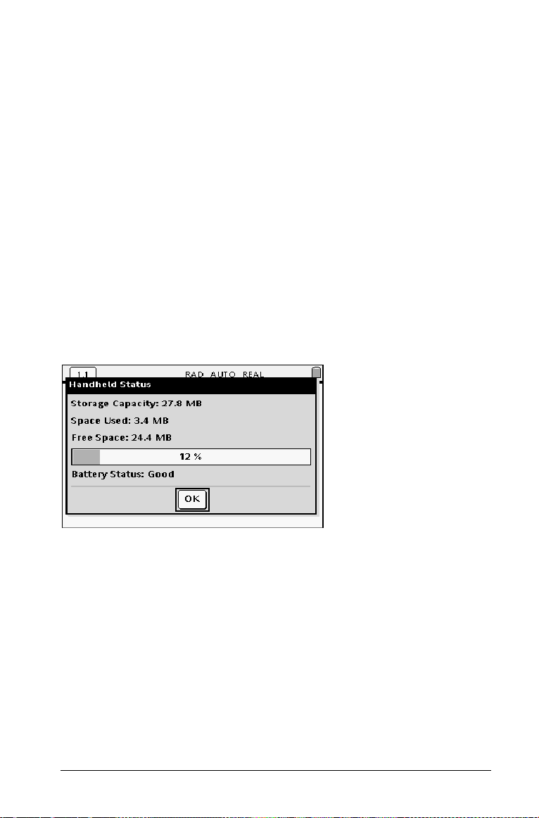
Checking available memory

The Handheld Status screen shows the amount of memory (in bytes) used by all documents and variables on your TI-Nspire™ CAS handheld. The Handheld Status screen displays the following information:

• Storage Capacity

•Space Used

• Free Space

• Battery Status

Displaying the Handheld Status screen

f Select Handheld Status from the Home menu.

c83

Press

The Handheld Status window displays.

Freeing memory

If you have insufficient memory to store documents on your handheld, you must free memory to create the space you need. To free memory, you must delete documents and/or folders from memory. If you wish to keep the documents and folders for use later, you can back them up to another handheld or to a computer.

Deleting items from memory

If you have documents stored on your TI-Nspire™ CAS handheld that you no longer need, you can delete them from memory to create additional space.

Memory and file management 15

Before you delete documents from memory, consider restoring sufficient available memory by copying files to another handheld.

1. Open

2. Press

3. Select

My Documents.

Press c7.

£ or ¤ to select the folder or document you want to delete.

Delete.

Press /c26.

The folder/document is permanently removed from the handheld.

Backing up files to another handheld

To back up files to another TI-Nspire™ CAS handheld, follow the steps below. Complete instructions for connecting two handhelds are provided in the Connectivity chapter.

1. Connect the two handhelds using the USB-to-USB Connectivity Cable.

2. Open

3. Press the 5 and 6 keys to highlight the document you want to send.

4. Select

5. When the file transfer is complete, a message displays on the

My Documents on the sending unit.

Press c7.

Send from the Document menu.

Press /c15.

receiving unit.

Backing up files to a computer

Use the TI-Nspire™ Computer Link software to back up the contents of your handheld to a computer. TI-Nspire™ Computer Link software is available on the product CD that came with your handheld.

Resetting the memory

The Reset button on the underside of the handheld resets all memory. When resetting all memory on the TI-Nspire™ CAS handheld, RAM and Flash memory is restored to factory settings. All files will be deleted. All system variables are reset to default settings.

Caution: Before you reset all memory, consider restoring sufficient available memory by deleting only selected data.

To reset all memory on the handheld, follow these steps.

16 Memory and file management

1. Use a paper clip or ball point pen to press the reset button on the underside of the handheld.

2. Hold for three seconds and release. Handheld memory is cleared.

When you clear memory, the contrast sometimes changes. If the screen is faded or blank, adjust the contrast by pressing

/+or /-.

Memory and file management 17

18 Memory and file management

Using Calculator

Getting started with the Calculator application

The Calculator application gives you a place to enter and evaluate math expressions. You can also use it to define variables, functions, and programs. When you define or edit a variable, function, or program, it becomes available to any TI-Nspire™ math and science learning technology application—such as Graphs & Geometry—that resides in the same problem.

You can also use Calculator to define library objects, such as variables, functions, and programs, which are accessible from any problem of any document. For information on creating library objects, see the “Libraries” section of the documentation.

À Calculator menu – This menu is available anytime you are in the

Calculator work area. Press this screen snapshot may not exactly match the menu on your screen.

b to display the menu. The menu in

Á Calculator work area

– You enter a math expression on the entry line and then press

· to evaluate the expression.

– Expressions display in standard mathematical notation as you

enter them.

Using Calculator 19

– Entered expressions and results show in the Calculator history.

Â Example of Calculator variables used in another application

The Calculator tool menu

The Calculator tool menu lets you enter and evaluate a variety of math expressions.

Menu Name

Actions

Number

Menu Option Function

Define Inserts the Define command.

Recall Definition Lets you view, reuse, or modify

a function or program that you have defined.

Delete Variable Inserts the

delVar command.

Clear a-z Deletes all variables with

single-letter names.

Clear History Deletes all expressions in the

Calculator history.

Insert Comment Lets you insert text.

Library Lets you refresh all libraries, set

LibPub or LibPriv access, insert a “\” character, or create a library shortcut.

Convert to Decimal

Inserts ¢Decimal command.

Factor Inserts factor().

Least Common Multiple Inserts

Greatest Common Divisor Inserts

Remainder Inserts

Fraction Tools Lets you select

20 Using Calculator

lcm().

gcd() function.

remain().

propFrac(), getNum(), getDenom(), or comDenom().

Menu Name

Algebra

Menu Option Function

Number Tools Lets you select round(), iPart(),

fPart(), sign(), mod(), floor(),

or ceiling().

Complex Number Tools Lets you select

imag(), angle(), ¢Polar, ¢Rect,

conj(), real(),

or the absolute value template.

Solve Inserts

Factor Inserts

solve().

factor().

Expand Inserts

Zeros Inserts

Numerical Solve Inserts

expand().

zeros().

nSolve().

Polynomial Tools Lets you select

polyRemainder(), polyQuotient(), polyGcd(), polyCoeffs(), or polyDegree().

Fraction Tools Lets you select

getNum(), getDenom(), or comDenom().

Convert Expression

Lets you select

propFrac(),

¢cos, ¢sin, or

¢Exp.

Trigonometry Lets you select tExpand() or

tCollect().

Complex Lets you select

cFactor(), or cZeros().

Extract Lets you select

Finance Solver Starts the Finance Solver.

Calculus

Derivative Inserts the Derivative template.

cSolve(),

left() or right().

Integral Inserts the Integral template.

Using Calculator 21

Menu Name

Menu Option Function

Limit Inserts the Limit template.

Sum Inserts the Sum template.

Product Inserts the Product template.

Function Minimum Inserts

fMin().

Function Maximum Inserts

Tangent Line Inserts

Normal Line Inserts

Arc Length Inserts

Series Lets you select

series(), or dominantTerm().

Differential Equation

Inserts

Solver

Implicit Differentiation Inserts

Numerical Calculations Lets you select

nfMin(), or nfMax()

Probability

Factorial (!) Inserts !.

Permutations Inserts

Combinations Inserts

Random Lets you select

randInt(), randBin(), randNorm(), randSamp(), or RandSeed.

fMax().

tangentLine().

normalLine().

arcLen().

taylor(),

deSolve().

impDif().

nDeriv(), nInt(),

nPr().

nCr().

rand(),

Distributions Lets you select from several

distributions, such as

, Binomial Cdf, and

Pdf Inverse F.

Statistics

22 Using Calculator

Normal

Menu Name

Menu Option Function

Stat Calculations Lets you select from several

statistics calculations, such as one-variable analysis, twovariable analysis, and regressions.

Stat Results Inserts the stat.results variable.

List Math Lets you select from several list

calculations, such as minimum, maximum, and mean.

List Operations Lets you select from several list

operations, such as sorting, filling, and converting to a matrix.

Distributions Lets you select from several

distributions, such as

, Binomial Cdf, and

Pdf Inverse F.

Normal

Confidence Intervals Lets you select from several

confidence intervals, such as

t interval and zinterval.

Stat Tests Lets you select from several

tests such as

test

ANOVA, t test, z

Matrix & Vector

Transpose Inserts T.

Inserts

det().

ref().

rref().

Determinant Inserts

Row-Echelon Form Inserts

Reduced Row-Echelon Form

Simultaneous Inserts

Using Calculator 23

simult().

Menu Name

Menu Option Function

Create Lets you select from several

matrix-creation options, such as construct matrix, identity, diagonal, submatrix, and others.

Norms Lets you select

rowNorm(), or colNorm().

norm(),

Dimensions Lets you select

rowDim(), or colDim().

Row Operations Lets you select

rowAdd(), mRow(), or mRowAdd().

dim(),

rowSwap(),

Element Operations Inserts “dot” operators such as

.+ (dot add) and .^ (dot power).

Advanced Inserts

Vector Inserts

trace(), LU, QR, eigVl(),

eigVc(), or charPoly(),

unitV(), crossP(), dotP(),

8Polar, 8Rect ,8Cylind, or 8Sphere.

Functions & Programs

Program Editor Lets you view, open for editing,

import, or create a new program or function.

Func...EndFunc Inserts a template for creating a

function.

Prgm...EndPrgm Inserts a template for creating a

program.

Local Inserts the

Local command.

Control Lets you select from a list of

function and program-control templates, such as

If...Then...EndIf, While...EndWhile, Try...Else...End Try, and others.

24 Using Calculator

Menu Name

Menu Option Function

Transfer Inserts transfer commands

Return, Cycle, Exit, Lbl, Stop,

or Goto.

Disp Displays intermediate results.

Mode Inserts commands for setting or

reading modes, such as display digits, angle mode, base mode, and others. Also lets you get the current language information.

Add New Line Starts a new line within a

function or program definition.

Before you begin

f Turn on the handheld, and add a Calculator application to a

document.

Entering and evaluating math expressions

Options for entering expressions

Calculator lets you enter and edit expressions through several methods.

• By pressing keys on the handheld keypad.

• By selecting items from the Calculator menu.

• By selecting items from the Catalog (

k).

Entering simple math expressions

Note: To enter a negative number on the handheld, press v. To enter a

negative number on a computer keyboard, press the hyphen key (

Suppose you want to evaluate

1. Select the entry line in the Calculator work area.

2. Type

Using Calculator 25

2^8 to begin the expression.

-).

3. Press ¢ to return the cursor to the baseline, and then type:

r 43 p 12.

4. Press · to evaluate the expression.

The expression displays in standard mathematical notation, and the result displays on the right side of the Calculator.

Note: If a result does not fit on the same line with the expression, it displays on the next line.

Controlling the form of a result

You might expect to see a decimal result instead of 2752/3 in the preceding example. A close decimal equivalent is 917.33333..., but that’s only an approximation.

By default, Calculator retains the more precise form: 2752/3. Any result that is not a whole number displays in a fractional or symbolic form (1/2,

p, , etc.). This reduces rounding errors that could be introduced by intermediate results in chained calculations.

You can force a decimal approximation in a result:

• By pressing

Pressing

• By including a decimal in the expression (for example,

43).

26 Using Calculator

· instead of · to evaluate the expression.

· forces the approximate result.

43. instead of

• By wrapping the expression in the approx() function.

• By changing the document’s Approximate.

– Press /c1 to display the File menu, and then select

Document Settings.

Note that this method forces all results in all of the document’s problems to approximate.

Auto or Approximate mode setting to

Inserting items from the Catalog

You can use the Catalog to insert system functions and commands, units, symbols, and expression templates into the Calculator entry line.

1. Press

k to open the Catalog.

Note: Some functions have a wizard that prompts you for each argument. If you prefer to enter the argument values directly on the entry line, you may need to disable the wizard.

2. Press the number key for the category of the item. For example, press 1 to show the alphabetic list.

Using Calculator 27

Contains all commands and functions, in alphabetical order.

Contains all math functions.

Provides the values for standard measurement units.

Provides a symbol palette for adding special characters.

Contains math templates for creating two dimensional objects, including product, sum, square root and integral.

Shows Public library (LibPub) objects.

3. Press ¤ and then use ¡, ¢, £, or ¤ as necessary to select the item

that you want to insert.

Note: To see syntax examples of the selected item, press then press the selected item, press

4. Press

· to alternately show or hide the Help. To move back to ge.

· to insert the item into the entry line.

e, and

Using an expression template

The Calculator has templates for entering matrices, piecewise functions, systems of equations, integrals, derivatives, products, and other math expressions.

For example, suppose you want to evaluate

1. Press

2. Select to insert the algebraic sum template.

28 Using Calculator

/r to open the Template palette.

The template appears on the entry line with small blocks representing elements that you can enter. A cursor appears next to one of the elements to show that you can type a value for that element.

3. Use the arrow keys to move the cursor to each element’s position, and type a value or expression for each element.

4. Press · to evaluate the expression.

Creating matrices

1. Press /r to open the Template palette.

2. Select . The Create a Matrix dialog box displays.

Using Calculator 29

3. Type the Number of rows.

4. Type the Calculator displays a template with spaces for the rows and columns. Note: If you create a matrix with a large number of rows and

columns, it may take a few moments to appear.

5. Type the matrix values into the template, and press · to define the matrix.

Number of columns, and then select OK.

Inserting a row or column into a matrix

f To insert a new row, press @.

f To insert a new column, hold down g and press ·.

Inserting expressions using a wizard

You can use a wizard to simplify entering some expressions. The wizard contains labeled boxes to help you enter the arguments in the expression.

For example, suppose you want to fit a y=mx+b linear regression model to the following two lists:

{1,2,3,4,5} {5,8,11,14,17}

1. Press

2. Press

3. Press ¤, and then press L to jump to the entries that begin with “L.”

4. Press

5. If the Use Wizard option is not checked:

30 Using Calculator

k to open the Catalog.

1 to show the alphabetic list of functions.

¤ as necessary to highlight LinRegMx.

a) Press

ee to highlight the Use Wizard button.

b) Press · to change the setting.

c) Press

6. Press

7. Type {

8. Press e to move to the Y List box.

9. Type

10. If you want to store the regression equation in a specific variable,

11. Select

·.

A wizard opens, giving you a labeled box to type each argument.

1,2,3,4,5} as X List.

{5,8,11,14,17} as Y List.

press e, and then replace Save RegEqn To with the name of the variable.

OK to close the wizard and insert the expression into the entry

line. Calculator inserts the expression and adds a statement to display the

variable stat.results, which will contain the results.

ee to highlight LinRegMx again.

LinRegMx {1,2,3,4,5},{5,8,11,14,17},1 : stat.results Calculator then displays the stat.results variables.

Using Calculator 31

Note: You can copy values from the stat.results variables and paste them into the entry line.

Creating a piecewise function

1. Begin the function definition. For example, type the following.

Define f(x,y)=

2. Press /r to open the Template palette.

3. Select . The Piecewise Function dialog box displays.

4. Type the

Number of Function Pieces, and select OK.

Calculator displays a template with spaces for the pieces.

5. Type the expressions into the template, and press · to define the function.

6. Enter an expression to evaluate or graph the function. For example, enter the expression

f(1,2) on the Calculator entry line.

Creating a system of equations

1. Open the Template palette.

32 Using Calculator

2. Select . The Create a System of Equations dialog box displays.

3. Type the

Number of Equations, and select OK.

Calculator displays a template with spaces for the equations.

4. Type the equations into the template, and press

Enter (·) to

define the system.

Deferring evaluation

You don’t have to complete and evaluate an expression as soon as you begin typing it. You can type part of an expression, leave to check some work you did on another page, and then come back to complete the expression later.

Working with variables

When you first store a value in a variable, you give the variable a name.

• If the variable does not already exist, Calculator creates it.

• If the variable already exists, Calculator updates it.

Variables within a problem are shared by TI-Nspire™ math and science learning technology applications. For example, you can create a variable in Calculator and then use or modify it in Graphs & Geometry or Lists & Spreadsheet within the same problem.

Exception: Variables created with the defined function or program are not accessible outside that function or program.

Local command within a user-

Storing a value in a variable

This example creates a variable named num and stores the result of the expression 5+8

1. On the Calculator entry line, type the expression

Using Calculator 33

in that variable.

5+8^3.

2. Press ¢ to expand the cursor to the baseline.

3. Press /h and then type the variable name num.

This means: Calculate 5+83 and store the result as a variable named num.

4. Press ·.

Calculator creates the variable num and stores the result there.

Alternative methods for storing a variable

As alternatives to using & (store), you can use “:=” or the Define command. All of the following statements are equivalent.

5+8

& num

num := 5+8

Define num=5+8

Checking a variable’s value

You can check the value of an existing variable by entering its name on the Calculator entry line.

f On the Calculator entry line, type the variable name

num and press

·.

The value most recently stored in num displays as the result.

Using a variable in a calculation

After storing a value in a variable, you can use the variable name in an expression as a substitute for the stored value.

34 Using Calculator

1. Type 4 r 25 r num^2 on the entry line, and press ·.

Calculator substitutes 517, the value currently assigned to num, and evaluates the expression.

2. Type

4 r 25 r nonum^2 on the entry line, and press ·.

Because the variable nonum has not been defined, it is treated algebraically in the result.

Updating a variable

If you want to update a variable with the result of a calculation, you must store the result explicitly.

Entry Result Comment

a := 2

a := a

& a

8 Result not stored in variable a.

2 8Variable a updated with result.

64 Variable a updated with result.

Types of variables

You can store the following TI-Nspire™ math and science learning technology data types as variables:

Data type Examples

Expression

2.54 1.25E6 2p 2+3i (xN2)

List {2, 4, 6, 8} {1, 1, 2}

Using Calculator 35

Data type Examples

Matrix

123

This can be entered as: [1,2,3;3,6,9]

369

Character string “Hello” “xmin/10” “The answer is:”

Function myfunc(arg) ellipse(x, y, r1, r2)

Entering multiple statements on the entry line

To enter several statements on a single line, separate them with a colon (“:”). Only the result of the last expression is shown.

Rules for naming variables

Note: In the unlikely event that you create a variable with the same

name as one used for statistical analysis or by the Finance Solver, an error condition could occur. If you begin entering a variable name that is already in use in the current problem, the software shows the entry in

bold to let you know.

• Variable names must be in one of the forms xxx or xxx.yyy. The xxx part can have 1 to 16 characters. The yyy part, if used, can have 1 to 15 characters. If you use the xxx.yyy form, both xxx and yyy are required; you cannot start or end a variable name with a period “.”

• Characters can consist of letters, digits, and the underscore character (_). Letters can be U.S. or Greek letters (but not Π or p), accented letters, and international letters.

• Do not use name such as c1 or n12. These may appear to be letters, but they are treated internally as special symbols.

• You can use uppercase or lowercase letters. The names AB22, Ab22, aB22, and ab22 all refer to the same variable.

• You cannot use a digit as the first character of xxx or yyy.

• Do not use spaces.

• If you want a variable to be treated as a complex number, use an underscore as the last character of the name.

c or n from the symbol palette to construct a variable

36 Using Calculator

• If you want a variable to be treated as a type of unit (such as _m or _ft), use an underscore as the first character of the name. You cannot

use subsequent underscores in the name.

• You cannot use a preassigned variable, function, or command name, such as Ans,

min, or tan.

Note: For a complete list of TI-Nspire™ functions, refer to the

Reference Guide.

• Library documents and library objects are subject to additional naming restrictions. For details, see the “Libraries” section of the documentation.

Here are some examples:

Variable names Valid?

Myvar, my.var Yes

My var, list 1 No. Contains a space.

a, b, c Yes

Log, Ans No. Preassigned to a system function or variable.

Log1, list1.a, list1.b Yes

3rdTotal, list1.1 No. xxx or yyy starts with a digit.

Reusing the last answer

Each instance of Calculator automatically stores the last calculated result as a variable named Ans. You can use Ans to create a chain of calculations.

Note: Do not link to Ans or any system variable. Doing so could prevent the variable from being updated by the system. System variables include statistics results (such as Stat.RegEqn, Stat.dfError, and Stat.Resid) and Finance Solver variables (such as tvm.n, tvm.pmt, and tvm.fv).

As an example of using Ans, calculate the area of a garden plot that is 1.7 meters by 4.2 meters. Then use the area to calculate the yield per square meter if the plot produces a total of 147 tomatoes.

1. On the Calculator entry line, type

2. Type

Using Calculator 37

147 p ans, and press · to find the yield.

1.7 r 4.2, and press ·.

As a second example, calculate and then add 2*log(45).

3. Type

4. Type

3.76 p (v7.9+sqrt(5)), and press ·.

ans+2 r log(45), and press ·.

Temporarily substituting a value for a variable

Use the “|” (such that) operator to assign a value to a variable for just a single execution of the expression.

Creating user-defined functions and programs

You can use the Define command to create your own functions and programs. You can create them in the Calculator application or in the Program Editor and then use them in other TI-Nspire™ applications.

For information on programming with the Program Editor, see the “Programming” and “Libraries” sections of the documentation.

Defining a single-line function

Suppose you want to define a function named cube() that calculates the cube of a number or variable.

1. On the Calculator entry line, type

Define cube(x)=x^3 and press

·.

38 Using Calculator

The message “Done” confirms that the function has been defined.

2. Type cube(2) and press · to test the function.

Defining a multiple-line function using templates

You can define a function consisting of multiple statements entered on separate lines. A multiple-line function may be easier to read than one with multiple statements separated by colons.

Note: You can create multiple-line functions only by using the command. You cannot use the := or & operators to create multiple-line definitions. The statements.

As an example, define a function named g(x,y) that compares two arguments x and y. If argument x > argument y, the function should return the value of x. Otherwise, it should return the value of y.

Func...EndFunc template serves as a container for the

Define

1. On the Calculator entry line, type yet.

2. Press

3. On the

4. Press

5. On the

Using Calculator 39

b to display the Calculator menu.

Functions & Programs menu, select Func...EndFunc.

Calculator inserts the template.

b to display the Calculator menu.

Functions & Programs menu, select Control, and then select

If...Then...Else...EndIf.

Calculator inserts the template.

Define g(x,y)=. Do not press ·

6. Type the remaining parts of the function, using the arrow keys to move the cursor from line to line.

7. Press

8. Evaluate

· to complete the definition.

g(3,-7) to test the function.

Defining a multiple-line function manually

Note: To start each new line without completing the function definition,

you press

As an example, define a function cumulative sum of integers from 1 through x. You can type the

underscore symbol by pressing

1. On the Calculator entry line, type

@ instead of pressing ·.

cum_sum(x) that calculates the

/_.

Define cum_sum(x)=. Do not press

· yet.

2. Press

3. On the

40 Using Calculator

b to display the Calculator menu.

Functions & Programs menu, select Func...EndFunc.

Calculator inserts the template.

4. Type the following lines, pressing @ at the end of each line.

5. After typing

6. Evaluate

Return tmpsum, press · to complete the definition.

cum_sum(5) to test the function.

Defining a program

Defining a program is similar to defining a multiple-line function. The

Prgm...EndPrgm template serves as a container for the program

statements.

As an example, create a program named arguments. Based on the comparison, the program should display the text “x greater than y” or “x not greater than y” (showing the values of x and y in the text).

1. On the Calculator entry line, type

g(x,y) that compares two

Define prog1(x,y)=. Do not press

· yet.

2. Press

3. On the

b to display the Calculator menu.

Functions & Programs menu, select Prgm...EndPrgm.

Calculator inserts the template.

Using Calculator 41

4. Press b to display the Calculator menu.

5. On the

If...Then...Else...EndIf.

Calculator inserts the template.

6. Type the remaining parts of the function, using the arrow keys to move the cursor from line to line. Use the Symbol Palette to type the ““ symbol.

7. Press

8. Execute

Functions & Programs menu, select Control, and then select

· to complete the definition.

prog1(3,-7) to test the program.

• Note: To stop a program or function manually, hold down the key for several seconds.

42 Using Calculator

Recalling a function or program definition

You might want to reuse or modify a function or program that you have defined.

1. Press

2. On the

3. Select the name from the list.

b to display the Calculator menu.

Actions menu, select Recall Definition.

A dialog box appears with a list of defined functions and programs.

The definition (for example, entry line for editing.

Define f(x)=1/x+3) is pasted into the

Editing Calculator expressions

Although you cannot edit an expression in the Calculator history, you can copy all or part of an expression from the history and paste it to the entry line. You can then edit the entry line.

Positioning the cursor in an expression

f Press e to cycle through the parameters of a template.

– or –

Press ¡, ¢, £, or ¤ to move the cursor through the expression. The cursor moves to the closest valid position in the direction that you

press.

Note: An expression template may force the cursor to move through its parameters, even though some parameters may not be exactly in the path of the cursor movement. For example, moving upward from the main argument of an integral always moves the cursor to the top limit.

Inserting into an expression in the entry line

1. Position the cursor at the point where you want to insert additional elements.

2. Type the elements that you want to insert.

Note: When you insert an open parenthesis, Calculator adds a temporary close parenthesis, displayed in gray. You can override the temporary parenthesis by typing the same parenthesis manually or by entering something past the temporary parenthesis (thereby implicitly validating its position in the expression). After you override the temporary gray parenthesis, it is replaced with a black parenthesis.

Using Calculator 43

Selecting part of an expression

1. Press ¡, ¢, £, or ¤ to move the cursor to a starting point.

2. Press and hold

g and press ¡, ¢, £, or ¤ to select.

Deleting all or part of an expression on the entry line

1. Select the part of the expression to delete.

2. Press ..

Financial calculations

Several TI-Nspire™ CAS functions provide financial calculations, such as time value of money, amortization calculations, and return on investment calculations.

The Calculator application also includes a Finance Solver. It lets you dynamically solve several types of problems, such as loans and investments.

Using the Finance Solver

1. Press b to display the Calculator menu.

2. On the The solver displays its default values (or previous values, if you have

already used the solver in the current problem).

Algebra menu, select Finance Solver.

3. Enter each known value, using e to cycle through the items.

– The help information at the bottom of the solver describes each

item.

– You might need to temporarily skip the value that you want to

calculate.

44 Using Calculator

– Make sure to set PpY, CpY, and PmtAt to the correct settings (12,

12, and END in this example).

4. Press e as necessary to select the item that you want to calculate, and then press ·.

The solver calculates the value and stores all the values in “tvm.” variables, such as tvm.n and tvm.pmt. These variables are accessible to all TI-Nspire™ CAS applications within the same problem.

Finance functions included

In addition to the Finance Solver, TI-Nspire™ CAS built-in finance functions include:

• TVM functions for calculating future value, present value, number of payments, interest rate, and payment amount.

• Amortization information such as amortization tables, balance, sum of interest payments, and sum of principal payments.

• Net present value, internal rate of return, and modified rate of return.

• Conversions between nominal and effective interest rates, and calculation of days between dates.

Notes:

• Finance functions do not automatically store their argument values or

results to the TVM variables.

• For a complete list of TI-Nspire™ functions, refer to the Reference

Guide.

Using Calculator 45

Working with the Calculator history

As you enter and evaluate expressions in the Calculator application, each entry/result pair is saved in the Calculator history. The history gives you a way to review your calculations, repeat a set of calculations, and copy expressions for reuse in other pages or documents.

Viewing the Calculator history

The history of the expressions you have entered accumulates above the entry line, with the most recent expression at the bottom. If the history does not fit in the Calculator work area, you can scroll through the history.

Note: You may notice a processing slowdown when the history contains a large number of entries.

f Press

£ or ¤.

À Scrollbar buttons Á Scroll position indicator Â Current entry/total entries

Reusing a previous expression or result

You can copy an expression, subexpression, or result from the Calculator history and paste it into the entry line or into other TI-Nspire™ applications.

1. Scroll to the item that you want to copy.

2. Select the item.

46 Using Calculator

Note: The float setting for the current document may limit the number of decimal places displayed in a result. To capture the result in its full precision, select it either by scrolling with the up and down arrow keys or by triple-clicking it.

3. Press

4. Select the location where you want the copy.

5. Press

Note: If you copy an expression that uses variables into a different problem, the values of those variables are not copied. You must define the variables in the problem where you paste the expression.

/C to make the copy.

/V to paste the copy.

Deleting an expression from the history

When you delete an expression, all variables and functions defined in the expression retain their current values.

1. Use the arrow keys to select the expression that you want to delete.

2. Press ..

The expression and its result are removed.

Clearing the Calculator history

When you clear the history, all variables and functions defined in the history retain their current values. If you clear the history by mistake, use the undo feature.

1. Press

2. On the

Using Calculator 47

b to display the Calculator menu.

Actions menu, select Clear History.

All expressions and results are removed from the history.

48 Using Calculator

Using Graphs & Geometry

Getting started with Graphs & Geometry

The Graphs & Geometry application enables you to:

• Graph and explore functions.

• Create and explore geometric shapes.

• Animate points on objects or graphs and explore their behavior.

• Graph data collected by the Data Collection tool.

• Explore graphical and geometric transformations.

• Explore and investigate concepts of calculus.

• Link to data created by other applications and utilize it in Graphs & Geometry.

ÁÂ

À Problem/Page number counter Á System Settings indicator Â Status indicator (with battery status indicator icon) Ã Graphs & Geometry units indicator (sample display is centimeters) Ä Sample Graphs & Geometry work area in Graphing View, with

Analytic Window and tooltip for triangle shown

Å Sample Graphs & Geometry entry line (line for function entry shown)

Getting acquainted with Graphs & Geometry

f Turn on the TI-Nspireé handheld, and add the Graphs & Geometry

application to your page.

Using Graphs & Geometry 49

When you add Graphs & Geometry to a page, your work area contains the x and y axes for a graph, as well as a function entry line and Graphs & Geometry-specific tools.

The basic components of the Graphs & Geometry application are the:

•Tool menu

• Work area (which contains the axes)

• Entry line.

The Tool menu

Press b to open the Actions menu. These menus and tools enable you to graph and explore different types of functions, draw and explore

geometric structures, as well as other capabilities which will be covered in this chapter.

The following tables contain a brief summary of what each menu contains or tool enables you to do within the Graphs & Geometry work area.

Note: The number that precedes each title is the numeric entry for accessing the tool using the handheld keys or the virtual keypad on the

computer. For example, to draw a circle, you would press

Menu Option List Overview of Tool Actions

1: Actions Provides tools to access the pointer, hide or

show various graph features, add text, delete all objects in the work area, access the calculate tool, and access the attributes for an object or function.

2: View Provides tools to manipulate the work area

features and display.

3: Graph Type Enables you to select the type of graph to

plot in the work area: function, parametric, polar, or scatter plot. The entry line below the work area shows the notational conventions to use to specify a function for the selected graph type.

4: Window Provides different Zoom settings as well as

the ability to define the x- and y-axis minimums and maximums.

b 8 1.

50 Using Graphs & Geometry

Menu Option List Overview of Tool Actions

5: Trace Creates and activates a trace on the graph.

Sets the trace increment and enables you to create and remove geometric trace.

6: Points & Lines Provides tools for drawing various types of

points, lines, segments, rays, tangents, vectors, and circle arcs.

7: Measurement Provides tools for measuring angles, lengths,

areas, integrals, and slope.

8: Shapes Provides tools for drawing circles, triangles,

rectangles, and polygons.

9: Construction Provides tools to define perpendicular and

parallel lines, bisectors, midpoints, locus, compass, and perform measurement transfers.

A: Transformation Provides tools for symmetry, reflection,

translation, rotation, and dilation.

Action Menu Tools

Tool name Tool function

1: Pointer Selects, moves, and manipulates

objects.

2: Select Enables you to select the objects in

part of the work area by placing a dashed-line box around them.

3: Hide/Show Enables you to hide or display any

object, function, or feature on the work area.

4: Attributes Enables you to change the attributes

of a selected object in the work area. Attributes vary depending upon the object selected.

5: Delete All Removes all objects and graphed

functions from the page.

Using Graphs & Geometry 51

Tool name Tool function

6: Text Places user-created alpha-numeric

values on the page. Numerical values can be applied to objects. The tool can be used to enter a function and graph it.

7: Coordinates and Equations

8: Calculate Opens the calculate tool to perform

9: Redefine Redefines a previously defined point

A: Insert Slider Lets you easily modify the value of a

Displays the coordinates of a point or the equation of a line or circle.

calculations using measurements, numerical values, or calculation results. This tool is different from the Calculator application.

to a new location. For example, it can define a point in free space to a location on an object or from one object to another object.

numeric variable.

View Menu Tools

Tool name Tool function

1: Graphing View Places the work area in graphing mode.

When you add Graphs & Geometry to a page the Cartesian axes displays in the work area with a function entry line below.

2: Plane Geometry View

3: Hide (Show) Analytic Window

Places the work area in geometry mode. Geometry scale displays, but no axes, grid, or entry line displays until you choose Show Analytic Window.

Opens a small graphing window on a plane geometry work area. Places the Graphs & Geometry work area in modeling mode. This tool can be used only after Plane Geometry is selected.

52 Using Graphs & Geometry

Tool name Tool function

4: Hide (Show) Axes Hides the axes if they are currently

displayed on the page. Displays the axes if none are displayed on the page.

5: Show (Hide) Grid Turns the grid on or off on the page.

Objects can be attached to the grid when the grid is displayed.

6: Hide (Show) Entry Line

7: Show (Hide) Scale Toggles between showing and hiding the

Show (Hide) Axes End Value

8: Add Function Table Launches the Lists & Spreadsheet

Hides or displays the entry line on the page.

scale legend on the work area. When the scale is shown, the value and/or units can be changed to desired values/units. This applies only to geometric constructions.

Toggles between showing and hiding the lowest value and highest value on the horizontal and vertical axes.

function table. When launched from Graphs & Geometry, it is pre-populated with all functions defined in the problem with the exception of hidden functions. More information on using Function Tables is available in the Lists & Spreadsheet chapter of this document.

Graphing Type Menu Tools

Tool name Tool function

1: Function Displays the function mode entry line at

the bottom of the work area.

2: Parametric Displays the parametric mode entry line

at the bottom of the work area. This display shows the t-min, t-max, and t-step values. The defaults are 0-2p max, and p/24 for t-step.

Using Graphs & Geometry 53

for t-min, t-

Tool name Tool function

3: Polar Displays the Polar mode entry line at the

bottom of the work area. This display shows the q-min, q-max, and q-step values. The defaults are 0-2p for q-min and q-max, and p/24 for q-step.

4: Scatter Plot Displays the Scatter Plot mode entry line

at the bottom of the work area.

Window Menu Tools

Tool name Tool function

1: Window Settings Lets you specify the minimum and

maximum values for the x-axis and yaxis. You can also set the axis scaling increment between tics.

2: Zoom - Box Enables you to define an area that

you want to enlarge.

3: Zoom - In Enables you to define the center

point of the zoom in location. The Zoom In factor is approximately 2.

4: Zoom - Out Enables you to define the center

point of the zoom out location. The Zoom Out factor is approximately 2.

5: Zoom - Standard Automatically sets x-min, x-max, y-

min, and y-max to center the origin. The x and y scale factors are equal. This is the default axes setting when Graphs & Geometry is first added to a page.

6: Zoom - Quadrant 1 Automatically sets x-min, x-max, y-

min, and y-max to emphasize the first quadrant. The x and y scale factors are equal.

54 Using Graphs & Geometry

Tool name Tool function

7: Zoom - User If you have modified any window

settings (such as x-min), Zoom-User saves the present settings. If you have not modified any window settings since last selecting ZoomUser, Zoom-User restores those settings.

8: Zoom - Trig Automatically sets x-min and x-max

to integer multiples of p. The x and y scale factors are equal.

9: Zoom - Data Redefines the axes so that all

statistical data points are displayed.

A: Zoom - Fit Recalculates y-min and y-max to

include the minimum and maximum y values of all functions between the current x-min and x-max. Hidden functions are not included.

B: Zoom - Square Recalculates y-min and y-max so that

the vertical scale is the same as the horizontal scale.

Trace Menu Tools

Tool name Tool function

1: Graph Trace Activates a trace point on the graph,

enabling you to trace functions.

2: Trace Setting Enables you to set the increment

between points touched by Graph Trace automatically, or by specifying a numeric trace step value.

3: Geometry Trace Enables you to view the pathway of a

geometric or analytic object (such as a function graph) on the work area. The pathway has a delayed fade. As more movement occurs on the work area, older portions of the pathway fade. If you temporarily halt movement, a portion of the trace path remains displayed.

Using Graphs & Geometry 55

Tool name Tool function

4: Erase Geometry Trace Halts geometric trace and erases all

persistent pathways on the work area.

Points and Lines Menu Tools

Tool name Tool function

1: Point Constructs a point defined in free space,

on an object, or at the intersection of two objects.

2: Point On Constructs a point defined on an object.

When the object is a function graph, the coordinates are displayed.

3: Intersection Point(s) Constructs a point at each intersection of

two selected objects.

4: Line Constructs an infinite line defined by

two points or by a point and a direction. If you press you limit its orientation, relative to the

x-axis or the horizontal aspect of the screen, by 15- increments.

5: Segment Constructs a segment, defined by two

end points, which may be created or defined in free space or on a defined object.

g while creating the line,

6: Ray Constructs a ray, defined by two points

or by a point and a direction, extending infinitely. If you press

the ray, you limit its orientation, relative to the x-axis or the horizontal aspect of the screen, by 15- increments.

7: Tangent Creates a tangent line.

8: Vector Constructs a vector with magnitude and

direction defined by two points.

9: Circle arc Creates an arc based on three points.

56 Using Graphs & Geometry

g while creating

Measurement Menu Tools

Tool name Tool function

1: Length Displays the distance between two

selected points or the length of a segment, perimeter, circumference, or radius.

2: Area Displays the area of a selected polygon

or circle.

3: Slope Displays the slope of a selected line or

segment. A vertical slope is represented by %.

4: Angle Displays the measure of an angle or an

angle defined by three selected points.

5: Integral Calculates and displays the numerical

value of the integral of a selected function, and shades the area between the curve and the x-axis from point a to point b.

Shapes Menu Tools

Tool name Tool function

1: Circle Constructs a circle. The center point is

defined by the first click on the page and the radius is determined by the second click.

2: Triangle Constructs a triangle, defined by three

points (vertices), which may be created or defined in free space or on a defined object.

3: Rectangle Constructs a rectangle.

4: Polygon Constructs an n-sided polygon. Each click

defines a vertex, and the polygon is completed by clicking the initial vertex or

by pressing

5: Regular Polygon Constructs an n-sided regular polygon.

Using Graphs & Geometry 57

·.

Construction Menu Tools

Tool name Tool function

1: Perpendicular Constructs a line perpendicular to a

selected line, segment, ray, vector, axis, or side of a polygon, and passing through a created or selected point.

2: Parallel Constructs a line parallel to a selected

line, segment, ray, vector, axis, or side of a polygon, and passing through a created or selected point.

3: Perpendicular Bisector Constructs a perpendicular line that

bisects two points, a segment, or side of a polygon.

4: Angle Bisector Constructs a line that bisects an angle

identified by three selected points where the second point is the vertex.

5: Midpoint Constructs a midpoint of two selected

points, a segment, or side of a polygon.

6: Locus Constructs the locus of a point or

object defined by the movement of a driver point along a pathway. Pathways are geometric shapes and function graphs.

7: Compass Constructs a circle from a center point

with a radius defined by a selected segment or the distance between two points.

8: Measurement transfer Transfers an entered or measured

value to a selected object, axis, or function graph. If the original value changes, the change is also reflected in the transferred measurement.

Transformation Menu Tools

Tool name Tool function

1: Symmetry Creates the image of an object rotated

- around a point.

180

58 Using Graphs & Geometry

Tool name Tool function

2: Reflection Creates the image of an object reflected

across a line, segment, ray, vector, axis, or side of a polygon.

3: Translation Creates the image of an object translated

by a specified vector.

4: Rotation Creates the image of an object rotated

around a point by a specified angular value.

5: Dilation Creates the image of an object dilated

from a point by a specified factor.

Note: When you select a tool to use, that tool’s icon displays in the upper left corner of the Graphs & Geometry page. It is there to remind you which tool is currently active.

Using the context menu

The context menu provides the tools most commonly used with the selected object, function, or axes.

To display the context menu for an object:

f Move the cursor to the object and then press /b. The first two options on the context menu are:

Recent: lists the 9 most recent tools you used. This is a session-level

• listing. The tools used on any Graphs & Geometry page are shown, regardless of the document in which they are used.

• Attributes: enables you to access the attributes appropriate for a selected function, object, or work area.

Additional options that are appropriate for your selection also display on the menu. For example, the context menu for a triangle also contains the Hide/Show, Delete, Length, and Area options.

The following examples show the context menu for a function and a circle.

Using Graphs & Geometry 59

Context menu for a function (analytic object)

Context menu for a geometric object

The work area

There are two work area views available:

• Graphing View

• Plane Geometry View

The Graphing view

The Graphing view is the default Graphs & Geometry work area display. It contains:

• the default Cartesian axes in the Zoom Standard format (1:1 scale).

• the entry line from which you can graph up to 100 functions.

Axes, entry line, and grid can all be displayed or hidden, but in this view, no scale for any drawn shapes (e.g. Circle, etc.) can be displayed. All objects created in this view are analytic objects. Therefore, their displayed size and proportion are affected only by the scale of the axis system (the command "Show Scale" has no effect).

60 Using Graphs & Geometry

The Plane Geometry view

The plane geometry view removes the axes and entry line from the work area to enable you to draw geometric shapes and explore them. In this view, you can display and set a scale for your drawings.

To change to Plane Geometry view:

1. From the View menu, select Plane Geometry View.

Press b 2 2.

2. The display refreshes to clear the axes and entry line and display a default scale. Any graphs or drawings created in graphing view are not displayed on the plane geometry area.

To return to Graphing view:

f From the

Press

The display refreshes to show the axes and entry line. Note: Any geometric constructions created while in the plane

geometry view are retained and displayed along with any previouslycreated graphs.

View Menu, select Graphing View.

b 2 1.

Using Graphs & Geometry 61

The analytic window

The analytic (graphing) window is available in the Plane Geometry view. It adds an analytic (graphing) window on top of a portion of the plane geometry work area. This provides a combination work area that enables you to use both work area types without toggling the view between them.

To open the analytic window:

1. Ensure that the work area is in Plane Geometry view.

2. From the View menu, select Show Analytic Window .

Press b 2 3.

3. A reduced size graphing window opens on the lower left corner of the plane geometry space.

62 Using Graphs & Geometry

Graphing area

Modeling view - shows the previous two views and the work done on both.

Plane Geometry area

You can alter the work area, without changing the view, to temporarily:

• Hide the axes. Any graphs or objects remain displayed on the work area.

• Show or hide axis end values and show or hide a grid in the graphing window.

• Hide the entry line.

• Hide the scale.

• Resize the axes using the zoom tools or by dragging tic marks.

To display more of the plane geometry work area, pan the screen.

To remove the analytic window from the work area

1. From the View menu, select Hide Analytic Window .

Press b 2 3.

Object behavior in different views

When you create an object in the graph area, it is called an analytic object, and all points of the object reside on the graph plane. When you change the axes scale, you automatically affect the appearance of the object. If you calculate a value associated with the object such as the area, only generic units are assigned (u for unit). These objects remain associated with the coordinate plane until you delete them or redefine them to the plane geometry area. When working with a modeling view work area, you cannot move an analytic object onto the plane geometry area.

Using Graphs & Geometry 63

When you create an object in the plane geometry area, it is a geometric object. These objects can have an assigned scale, such as miles or centimeters, instead of u for units. You can lock a point, such as one vertex of a triangle, on the work area, but since the object is not tied to a coordinate plane, you cannot display coordinates for that vertex. When working with a modeling mode work area (Plane Geometry view with analytic window), you can move a geometric object into the graphing work area. The object remains a geometric object, and is not associated with the axes.

The examples below show a modeling work area and the two types of objects: A is an analytic object while B is a geometric object.

While the two circles appear identical, they do not behave in the same way. Analytic objects are impacted when the graph area is altered. In the next example, the axes were altered. Notice that only Circle A’s appearance is affected by the change.

64 Using Graphs & Geometry

If you construct an object while the axis is hidden, the object created will be a geometric object. However, if you construct an analytic object and later hide the axis, the object remains an analytical one.

Triangle as it appears in Graphing view. The unlabeled vertex remains a geometric point.

Using Graphs & Geometry 65

Summary of differences

Feature Graph Area Plane Geometry Area

Aspect Ratio Adjustable; initially 1:1 Always 1:1 (static)

Units of Measure Generic (displayed as u) User-defined (per scale)

Area Graph Type Cartesian (default) or

Polar

Uses • Define and graph

functions to: – Graph

functions of the form f (x)

– Create scatter

plots

– Graph polar

equations

– Graph

parametric functions

• Construct analytic objects

• Label equations

• Identify coordinates for discrete points

Behavior Analytic constructions

must remain in the analytic area.

Euclidian

• Construct Euclidean objects

• Create transformations

• Determine measurements (for example, length, angle, or area)

Geometric constructions can be moved into the analytic area but remain geometric in nature.

Creating and manipulating axes

When you add the Graphs & Geometry application to a page, Cartesian axes displays by default.

You can change the appearance of your axes in the following ways:

1. Adjust the length of the axes:

• When using Plane Geometry view with Show Analytic Window, – Select an axis and retype the domain or range labels.

66 Using Graphs & Geometry

– Select an axis and drag to increase or decrease the numbers

on the scale and tic mark spacing.

The aspect ratio of the axes is retained. To modify the scale of only one axis, press

Extended domain

g as you adjust the value or drag the line.

Default range and domain

2. Use the Zoom tool options to adjust the view.

3. Adjust the end style of the axes using the Attributes tool. Display the Attributes tool by:

• selecting it from the menu or

• pressing

Press the left and right arrow keys to display the desired end style. The attributes list for the axes also enables you to select a Zoom tool.

4. Adjust the axes scale and tic mark spacing manually.

a) Click and hold one tic mark, and move it on the axis. The

b) To adjust the scale and tic mark spacing on a single axis,

Using Graphs & Geometry 67

/ and clicking an axis between two tick marks.

spacing and number of tic marks increases (or decreases) on both axes.

press and hold that axis.

g, and then grab and drag a tic mark on

5. Change axis end values by double-clicking them and typing new values.

6. Adjust the location of the axes. To move the existing axes without resizing or rescaling them, click in and drag an empty region of the screen until the axes are in the desired location.

7. Use the Window Setting tool to define the x-max, x-min, y-max, y-min, x-scale and y-scale values for the axes. When selected, this tool opens a dialog that enables you to enter the values desired. The current values are initially displayed. Type over them to enter new values.

Window Settings dialog with initial values displayed

Note: The axis values set on the Window Settings dialog can be stored as variables that can be accessed outside of Graphs & Geometry. Select the axis label at the value to be linked, and then click

You can use tools on the

View menu to hide and redisplay the axes, the

var to link to the value.

scale, and axis end values.

f From the

View menu, select Hide/Show Axes .

Press b24.

• If the axes are shown on the page, selecting this tool hides them.

• If the axes are hidden on the page, selecting this tool redisplays

them.

68 Using Graphs & Geometry

Moving about the work area

Graphs of functions may extend beyond the visible portion of your screen. This does not mean they are truncated. You can view them by panning the screen. To pan the screen:

1. Click and hold the mouse button in an open area of the page.

2. Move to display different portions of the screen.

Turning the grid on or off

Graphs & Geometry can display a grid in addition to the axes for a function. You control the sizing of the grid as well as whether or not it is visible.

To display the grid:

f From the

Pressb 2 5.

View menu, select Show Grid .

Using Graphs & Geometry 69

You resize the grid by rescaling the axes.

To turn the grid off:

f From the

View menu, select the Hide Grid .

Press b25.

When the tool is selected, the page updates to remove the grid.

In addition, you can attach a function, graph, or object to the grid while the grid is displayed.

Attaching an object to the grid

1. Display the grid on the page if it is not already present.

2. Draw an object on the grid. Positioning the object so that points coincide with grid marks attaches the object to the grid.

For example, if you draw a triangle, then one or more of the vertices must coincide with grid marks.

Note: You do not have to attach an object or graph to the grid. When you attach an object to the grid, its subsequent relocation is constrained to other grid points. Analytic objects are affected by axes changes regardless of whether or not they are attached to the grid.

To unattach an object from the grid, select and redefine it so that points do not coincide with grid marks. If you hide the grid, objects attached to it remain displayed on the page and remain attached to the grid even though it is no longer visible.

70 Using Graphs & Geometry

The Zoom feature

For screens with many function graphs, it can be difficult to view intersections and other areas of interest. To temporarily change your view of the screen, use the Zoom feature.

To use Zoom:

1. Open the Window menu.

Press b4.

2. Click the Zoom tool you want to use. In the following examples, all options except Zoom-Fit started with

the graph of x The options are:

• Zoom - Box

Press b42.

. Zoom-Fit shows a graph of a sine function.

•Zoom - In

Press b43.

• Zoom - Out

b44.

Press

Using Graphs & Geometry 71

• Zoom - Standard

Press b45.

•Zoom - Quadrant 1

b46.

Press

• Zoom - User (appears the same as Zoom - Standard if no new configuration is saved)

b47.

Press

72 Using Graphs & Geometry

•Zoom - Trig

Press b48.

• Zoom - Data

Press b49.

• Zoom - Fit

b4A.

Press

Using Graphs & Geometry 73

• Zoom - Square

Press b4B.

Circles before Zoom - Square

3. The graph displays in the selected zoom view. If you select

the box. If you select either Zoom In or Zoom Out, you must click the center

point before the graph is redrawn.

4. To return the graph to its initial state, either select

Zoom - Standard from the Zoom menu.

Zoom Box, you must click the first and third corners of

Circles after Zoom - Square

Undo or select

The entry line

The Entry line appears at the bottom of the Graphs & Geometry work area. When the line is not active, it is grayed out.

ÀÁ Â Ã Ä

From left to right, the parts of this line are:

À Hide/Show button. Á Attributes button.

74 Using Graphs & Geometry

Â f1(x)= is the default notation for a function or inequality. Ã Blank area into which you enter the function, polar equation,

inequality, parametric, or scatter plot data to be graphed.

Ä Expand/Contract (History) button.

Parametric Mode entry line

Scatter Plot Mode entry line

Polar Mode entry line

Using Graphs & Geometry 75

Additional Graphs & Geometry features

Keystroke shortcuts

There are keystroke shortcuts that can simplify your work with Graphs & Geometry. These are:

Keystrokes: Task accomplished:

+ (+) - (-)

< > When a number is under the pointer, the < and >

Using the tab and arrow keys

While the pointer allows you to access the many features and tools contained in Graphs & Geometry, you can also use the e and arrow keys to access these features. Using these keys is easier or more

convenient than using the pointer.

Removes a selected object from the work area.

When used with the Line or Circle tool, constrains Circle and some linear objects (Line and Ray) to discrete intervals (for example, Circle to integer radius values and linear objects to multiples of 15 degrees).

When a number is under the pointer, the + and keys enable you to change the number of displayed digits.

keys decrease or increase a value.

e key:

The

• First tab stop: places the cursor to the right of the equal sign on the function entry line. This allows you to create a new expression.

• Second tab stop: highlights the Expand/Collapse entry line History button.

• Third tab stop: highlights the Hide/Show button on the entry line.

• Fourth tab stop: highlights the Attributes button on the entry line.

• Fifth tab stop: focuses on the Pause/Start button of the animation control bar, if present. If the Data Collection control bar is displayed, focuses on the Start/Stop button.

• Sixth tab stop: focuses on the graphing portion of the page and commits any editing changes. The pointer is active on the page.

Note: Press ge to move through the steps in reverse order. If slider controls are included on the work area, the fifth tab stop

76 Using Graphs & Geometry

moves to the slider control. Press Esc to jump to a graph on the work area at any time.

The arrow keys:

• Up and Down - moves up and down among functions in the function history list. Moves up and down any tool menu list as well as the attributes list. When using the Trace tool, enables you to move to and trace a different graph when more than one graph is on the page.

• Left and Right - moves along the entry line, one space or one button at a time. When using the Trace tool, moves the trace cursor along the graph, either left or right. When viewing an attribute list, steps through the options for one attribute.

Using Sliders

Sliders let you easily change the value of a numeric value in the Graphs & Geometry and Data & Statistics applications. Inserting a slider lets you represent multiple variable values in a continuous range. In the following example, the slider represents the numeric variable, b in the graphed function.

f To insert a slider, select Insert Slider on the Actions menu. The

slider displays on the work area.

À Variable statement that includes the name of a numeric variable in

an entry field, the assignment operator":=", and the value set for the numeric variable in a second entry field

Using Graphs & Geometry 77

Á Slider that you can move to values on the scale when the control is

active

Â Track with labels for the minimum and maximum values on the scale

and scale tic marks between the end values

Basic slider operation

To change the default variable name (v1), click the text box on the left, highlight the default name, and type the name of the variable that you want the slider to represent. You can move the slider to set the variable to a value, or type a number in the text box after the equal sign. Press or click another part of the work area to unselect a slider.

You can use a slider in the following ways:

• Grab the slider and drag it to set the variable to any value within its range.

• Click a point near the slider track to grab the entire control for operations such as copying, moving, and deleting.

• Drag the track ends to change the length of the slider scale.

• Click the text box for the slider variable name and type the name of the numeric variable to use. You can use an existing numeric variable or use the slider to create a new one.

Context menu and slider settings

To change the settings for a slider, access the slider context menu:

Esc

Select Settings to display the Slider Settings dialog:

78 Using Graphs & Geometry

Specify the values to use for the slider:

Variable Sets the name of the numeric variable used with the slider.

Type the value in the field or click the drop-down arrow to select a value from the list.

Initial value Sets the starting value of the variable.

Minimum Sets the lowest value in the range of values used with the

slider. This value displays at the left end of the scale.

Maximum Sets the highest value in the range of values used with the

slider. This value displays at the right end of the scale.

Step Size Sets the size of the increment between values. When a

slider is active, you can use the arrow keys to move the slider up or down the scale by this amount.

Style Lets you choose how the slider is displayed in the work

area. Choose horizontal for a left-to-right scale, or choose vertical for a top-to-bottom scale. To display a slider that includes the variable name, current value, and direction arrows only, choose minimized.

Result Lets you choose the format for the displayed value of a

slider. Choose Auto to let slider operate in the default format, or choose from eight floating point formats.

Show variable

Shows or hides the variable.

Show scale Shows or hides the scale on the slider track.

Animating a slider

From the slider context menu, click Animate to step through the variable range automatically. To stop the animation, click Stop Animate.

Minimizing a slider

From the slider context menu, click Minimize to show a smaller display that includes the variable name, the current value of the variable, and up and down arrows.

Minimized

Using Graphs & Geometry 79

Opening and exporting files

You can open Cabri II Plus™ Figures (.fig) files in Graphs and Geometry and open TI-Nspire™ .tns files in Cabri II Plus™ software. Cabri II Plus™ files that you open in Graphs & Geometry convert to a Graphs & Geometry page with converted figures and a Notes page with conversion messages. Each Graphs & Geometry page converts to a separate Cabri II Plus™ file when you open a .tns document in Cabri II Plus™ software.

Note: On a Macintosh computer, you cannot open a Cabri II Plus™ .fig file or a Learning Check .edc file. You also cannot export a TI-Nspire .tns document as a .fig file.

Opening a Cabri II Plus™ file

To open a Cabri II Plus™ figures (.fig) file in Graphs & Geometry:

1. Select Open Document on the

2. On the Open TI Nspire Document dialog, click Files of Type and choose Cabri Plus II Figures (*.fig).

3. Click the .fig file that you want to open in Graphs & Geometry and click Open.

Converted Cabri II Plus™ figures display on a Graphs and Geometry page and conversion messages display on a Notes page. The file is saved as a .tns document.

File menu.

Exporting a Cabri II Plus™ file

To export Graphs & Geometry pages of a TI-Nspire™ .tns document to Cabri II Plus™ software:

1. Open the .tns file that contains the Graphs & Geometry pages to export.

2. Choose Export on the File menu.

3. On the Export to Cabri dialog, click OK to save the .fig files in the current folder.

Each Graphs & Geometry application in the document will be converted to a separate Cabri II Plus™ file within that folder.

Attribute settings

The following table lists the attributes available when working with objects. The list of available attributes depends upon the object you

select. To view attributes, select the Attributes tool .

80 Using Graphs & Geometry

When the tool is selected, move the cursor to the work area and select the object or function whose attributes you want to change. The column of attributes available displays on the work area near the object or function.

Name Icon(s) Options Available for use on

Line Weight

Thin, Medium, Thick

Line, Tangent, Segment, Ray, Vector, Circle, Circle arc, Triangle, Polygon, Regular Polygon, Rectangle, Graphed Functions, Integrals, Polar Equations, Parametric plots

Line Style

Animation

Fill

Lock/ Unlock

Solid, Dashed, Dotted

Unidirectional Animation Speed, Alternating Animation Speed

No fill, White, Light Grey, Med Grey, Grey, Dark Grey, Black

Line, Tangent, Segment, Ray, Vector, Circle, Circle arc, Triangle, Polygon, Regular Polygon, Rectangle, Graphed Functions, Polar Equations, Integrals, Parametric Plots

Point, Point On

Circle, Triangle, Polygon, Regular Polygon, Rectangle, Integrals

Point, Point On, Intersection Point, Length, Perimeter, Area, Angle

Using Graphs & Geometry 81

Name Icon(s) Options Available for use on

Point Style

Small dot, Large dot, Hollow circle,

Point, Point On,

Intersection Point Solid square, Hollow square, x, +

Activation

Graph Appearance

Axes Style

Axes Settings

Axes End Style

Axes Tic Labels

Axes End Values

Line Equation Type

Point Activated, Point Deactivated

Continuous, Discrete, Number of Points, Step Size

Grid, No Grid Axes

Axes user settings, Axes Quadrant 1 settings, Axes Trig settings, Axes Stat settings, Axes standard settings

No Arrow, Positive Arrows, All Arrows

Tic labels are shown, Tic labels are hidden

End Values are shown, End Values are hidden

Cartesian (y=_), Canonical (_=0)

Points

Graphed Functions,

Polar Equations,

Parametric Curves

Axes

Line, Tangent, Segment,

Ray, Vector

82 Using Graphs & Geometry

Name Icon(s) Options Available for use on

Equation Type

Canonical (...=0), Cartesian (...=r

Circle

)

Plot Points

Labels

Discrete Points, Connected Points

y=, f( ), f( )=, y=f( ), f,

Parametrics, Scatter Plots, Polar equations

Graphed Functions

Changing the thickness and style of a line/outline

You can control the thickness and appearance of the lines and outlines of shapes that you create on the screen. To adjust the thickness of the lines:

1. From the Actions menu, select the Attributes .

Press

b13.

2. Select the object whose line you want to change. Use 9 and : to move through the list of attributes.

3. Highlight the thickness option, and use 7 or 8 to move through the thickness options.

As you move through the options, the thickness immediately changes on the screen.

4. When the desired thickness displays on the screen, press to confirm the change.

The Attributes bar disappears.

Use the same method to change the style of the line, selecting the style attribute, instead of the thickness attribute.

· or click

Locking measured values and points

Graphs & Geometry allows you to lock one or many values or points. To do this:

1. From the

Press

Using Graphs & Geometry 83

Actions menu, select Attributes .

b13 .

2. Select the value or point that you want to lock.

3. Use 9 and : to locate the Lock attribute.

4. Use 7 or 8 to select

Lock.

5. Click or press · to lock the value or point.

A lock icon appears near the locked value or point.

An example of when locking measured values is useful is the problem of maximizing an area contained within a fixed perimeter. In this case, a rectangle is created with the correct perimeter, and both the perimeter and area values are displayed. The perimeter value is locked. As you alter the sides of the rectangle, the perimeter remains unchanged but the area changes. When the optimum area displays, you can measure the sides to obtain the necessary dimensions.

Initial rectangle with locked perimeter

Optimized area with same initial perimeter

Working with functions

The entry line under the work area lets you specify functions in the format supported for each graph type in Graphs & Geometry.

Using the entry line

The entry line displays at the bottom of the page. The entry line displays the form to use to type the function that corresponds to the selected graph type. To type details for a function on the entry line:

1. Select the graph type to set the graphing mode. You can specify multiple functions for each graph type. The default graph type is Function, so the form f1(x)= displays.

2. Type the data for the type of function you want to graph using the function formatting that displays on the entry line:

84 Using Graphs & Geometry

– To graph a function, select Function on the Graph Type menu.

The work area and entry line change to function mode. Enter an expression for the function after the equal sign.

b31.

Press

– To graph a parametric equation, select

area and entry line change to parametric mode. Type expressions for xn(t) and yn(t). Specifying alternate values for the default t-min, t-max, and t-step displayed is optional.

b32.

Press

– To graph a polar equation, select

line change to polar mode. Type an expression for rn(q). Specifying alternate values for the default q-minimum and q- maximum, and q-step displayed is optional.

b33.

Press

Parametric. The work

Polar. The work area and entry

– To graph a scatter plot, select

entry line change to scatter plot mode. Click the arrows that display to choose x and y for sn.

Press b34.

3. Press

After your selection is graphed, the entry line changes to enable you to specify another graph of the same type. For example, after you graph f1(x), the entry line changes to f2(x)= to enable you to enter another function. If you select or trace a function, that function displays on the entry line.

As you graph multiple functions on one set of axes, Graphs & Geometry labels each with its function. You can define and graph a maximum of 99 functions of each type. For example, you use function mode to specify functions (f1(x) - f99(x) ). You can also rename multiple functions that use custom names, for example, g1(x).

Note: If you draw a geometric figure, the entry line may disappear from the page. Press

· or e.

/G to select the Show Entry Line tool .

Scatter Plot. The work area and

Using the entry line expand button

Click the entry line to display a line-by-line history list of the functions entered on the screen. The list displays functions in the order of entry (top to bottom), with the most recent entry closest to the entry line. Use 9 and : to move up and down the list.

Using Graphs & Geometry 85

Use the function history to edit, change the attributes of, delete, or hide (or redisplay) a specific function or graph.

Graphing a family of functions

A family of functions differ by one or more parameters and can be specified with a single expression. To graph a family of functions:

1. Type an expression for a family of functions on the entry line. To specify a family of functions:

• Specify the parameters as one expression for multiple functions

using the format f1(x)={-1,0,1,2}*x+{2,4,6,8} or f1(x)=m*x| m={1,2,3}.

• Enclose the lists of numbers or lists of variables in curly brackets.

For example, four functions are denoted with the expression: f1(x)={-1,0,1,2}*x+{2,4,6,8}. The first function to be evaluated is y= -1 * x + 2 and the second is 0*x + 4.

86 Using Graphs & Geometry

Texas instruments TI-NSPIRE Learning and Technology Handheld Part 2

Specifications and Main Features

Frequently Asked Questions

User Manual

Important Information

Introduction

The TI-Nspire™ CAS math and science learning handheld

How to use this guidebook

Where to find more information

Transferring Files

Connecting two handhelds

Using connection cables

USB cables

Connecting two TI-Nspire™ CAS handhelds with the USB unit-to-unit cable

Backing up files to a computer

Transferring documents

Rules for transferring files

Sending a document

Receiving a document

Canceling a transfer

Upgrading the Operating System

Important Operating System download information

Where to get Operating System upgrades

Transferring the Operating System

Important:

OS Upgrade Messages

Memory and file management

Checking available memory

Displaying the Handheld Status screen

Freeing memory

Deleting items from memory

Backing up files to another handheld

Backing up files to a computer

Resetting the memory

Using Calculator

Getting started with the Calculator application

Before you begin

Entering and evaluating math expressions

Options for entering expressions

Entering simple math expressions

Controlling the form of a result

Inserting items from the Catalog

Using an expression template

Creating matrices

Inserting a row or column into a matrix

Inserting expressions using a wizard

Creating a piecewise function

Creating a system of equations

Deferring evaluation

Working with variables

Storing a value in a variable

Alternative methods for storing a variable

Checking a variable’s value

Using a variable in a calculation

Updating a variable

Types of variables

Entering multiple statements on the entry line

Rules for naming variables

Reusing the last answer

Temporarily substituting a value for a variable

Creating user-defined functions and programs

Defining a single-line function

Defining a multiple-line function using templates

Defining a multiple-line function manually

Defining a program

Recalling a function or program definition

Editing Calculator expressions

Positioning the cursor in an expression

Inserting into an expression in the entry line

Selecting part of an expression

Deleting all or part of an expression on the entry line

Financial calculations

Using the Finance Solver

Finance functions included

Working with the Calculator history

Viewing the Calculator history

Reusing a previous expression or result

Deleting an expression from the history

Clearing the Calculator history

Using Graphs & Geometry