Tektronix TDS420A, TDS430A, TDS460A, TDS510A User Manual

User Manual

TDS 420A, TDS 430A, TDS 460A & TDS 510A
Digitizing Oscilloscopes

070-9701-03

www.tektronix.com

Copyright © T ektronix, Inc. All rights reserved.
T ektronix products are covered by U.S. and foreign patents, issued and pending. Information in this publication supercedes

that in all previously published material. Specifications and price change privileges reserved.
T ektronix, Inc., P.O. Box 500, Beaverton, OR 97077
TEKTRONIX and TEK are registered trademarks of T ektronix, Inc.

WARRANTY

T ektronix warrants that the products that it manufactures and sells will be free from defects in materials and workmanship
for a period of three (3) years from the date of shipment. If a product proves defective during this warranty period,
T ektronix, at its option, either will repair the defective product without charge for parts and labor, or will provide a
replacement in exchange for the defective product.

In order to obtain service under this warranty, Customer must notify Tektronix of the defect before the expiration of the
warranty period and make suitable arrangements for the performance of service. Customer shall be responsible for
packaging and shipping the defective product to the service center designated by T ektronix, with shipping charges prepaid.
T ektronix shall pay for the return of the product to Customer if the shipment is to a location within the country in which the
T ektronix service center is located. Customer shall be responsible for paying all shipping charges, duties, taxes, and any
other charges for products returned to any other locations.

This warranty shall not apply to any defect, failure or damage caused by improper use or improper or inadequate
maintenance and care. T ektronix shall not be obligated to furnish service under this warranty a) to repair damage resulting
from attempts by personnel other than T ektronix representatives to install, repair or service the product; b) to repair
damage resulting from improper use or connection to incompatible equipment; c) to repair any damage or malfunction
caused by the use of non-T ektronix supplies; or d) to service a product that has been modified or integrated with other
products when the effect of such modification or integration increases the time or difficulty of servicing the product.

THIS WARRANTY IS GIVEN BY TEKTRONIX IN LIEU OF ANY OTHER WARRANTIES, EXPRESS OR
IMPLIED. TEKTRONIX AND ITS VENDORS DISCLAIM ANY IMPLIED WARRANTIES OF
MERCHANTABILITY OR FITNESS FOR A PARTICULAR PURPOSE. TEKTRONIX’ RESPONSIBILITY TO
REP AIR OR REPLACE DEFECTIVE PRODUCTS IS THE SOLE AND EXCLUSIVE REMEDY PROVIDED TO
THE CUSTOMER FOR BREACH OF THIS WARRANTY . TEKTRONIX AND ITS VENDORS WILL NOT BE
LIABLE FOR ANY INDIRECT , SPECIAL, INCIDENTAL, OR CONSEQUENTIAL DAMAGES IRRESPECTIVE
OF WHETHER TEKTRONIX OR THE VENDOR HAS ADVANCE NOTICE OF THE POSSIBILITY OF SUCH
DAMAGES.

Table of Contents

Getting Started

Operating Basics

Reference

General Safety Summary vii. . . . . . . . . . . . . . . . . . . . . . . . . . . . . . . . . . . .

Preface ix. . . . . . . . . . . . . . . . . . . . . . . . . . . . . . . . . . . . . . . . . . . . . . . . . . .

Product Description 1–1. . . . . . . . . . . . . . . . . . . . . . . . . . . . . . . . . . . . . . . . .

Start Up 1–3. . . . . . . . . . . . . . . . . . . . . . . . . . . . . . . . . . . . . . . . . . . . . . . . . .

Overview 2–1. . . . . . . . . . . . . . . . . . . . . . . . . . . . . . . . . . . . . . . . . . . . . . . . . .

At a Glance 2–3. . . . . . . . . . . . . . . . . . . . . . . . . . . . . . . . . . . . . . . . . . . . . . . .

Tutorial 2–11. . . . . . . . . . . . . . . . . . . . . . . . . . . . . . . . . . . . . . . . . . . . . . . . . . .

Overview 3–1. . . . . . . . . . . . . . . . . . . . . . . . . . . . . . . . . . . . . . . . . . . . . . . . . .

Accessing Help 3–3. . . . . . . . . . . . . . . . . . . . . . . . . . . . . . . . . . . . . . . . . . . . .

Acquisition Modes 3–5. . . . . . . . . . . . . . . . . . . . . . . . . . . . . . . . . . . . . . . . . .

Delayed Triggering 3–11. . . . . . . . . . . . . . . . . . . . . . . . . . . . . . . . . . . . . . . . .

Determining Status 3–15. . . . . . . . . . . . . . . . . . . . . . . . . . . . . . . . . . . . . . . . .

Display Modes 3–17. . . . . . . . . . . . . . . . . . . . . . . . . . . . . . . . . . . . . . . . . . . . .

Edge Triggering 3–21. . . . . . . . . . . . . . . . . . . . . . . . . . . . . . . . . . . . . . . . . . . .

Fast Fourier Transforms (Optional) 3–27. . . . . . . . . . . . . . . . . . . . . . . . . . .

File System 3–43. . . . . . . . . . . . . . . . . . . . . . . . . . . . . . . . . . . . . . . . . . . . . . . .

Hardcopy 3–47. . . . . . . . . . . . . . . . . . . . . . . . . . . . . . . . . . . . . . . . . . . . . . . . .

Horizontal Control 3–55. . . . . . . . . . . . . . . . . . . . . . . . . . . . . . . . . . . . . . . . .

Limit Testing 3–63. . . . . . . . . . . . . . . . . . . . . . . . . . . . . . . . . . . . . . . . . . . . . .

Logic Triggering (TDS 510A Only) 3–67. . . . . . . . . . . . . . . . . . . . . . . . . . . .

Measuring Waveforms 3–73. . . . . . . . . . . . . . . . . . . . . . . . . . . . . . . . . . . . . .

Probe Cal (TDS 510A Only) 3–83. . . . . . . . . . . . . . . . . . . . . . . . . . . . . . . . . .

Probe Compensation 3–89. . . . . . . . . . . . . . . . . . . . . . . . . . . . . . . . . . . . . . . .

Pulse Triggering (TDS 510A Only) 3–91. . . . . . . . . . . . . . . . . . . . . . . . . . . .

Remote Communication 3–97. . . . . . . . . . . . . . . . . . . . . . . . . . . . . . . . . . . . .

Roll Mode (TDS 400A Only) 3–99. . . . . . . . . . . . . . . . . . . . . . . . . . . . . . . . .

Saving and Recalling Setups 3–103. . . . . . . . . . . . . . . . . . . . . . . . . . . . . . . . . .

Saving and Recalling Waveforms 3–105. . . . . . . . . . . . . . . . . . . . . . . . . . . . .

Selecting Channels 3–111. . . . . . . . . . . . . . . . . . . . . . . . . . . . . . . . . . . . . . . . . .

Setting Up Automatically: Autoset and Reset 3–113. . . . . . . . . . . . . . . . . . .

TDS 420A, TDS 430A, TDS 460A & TDS 510A User Manual

i

Table of Contents

Appendices

Glossary

Signal Path Compensation 3–115. . . . . . . . . . . . . . . . . . . . . . . . . . . . . . . . . . .

Taking Cursor Measurements 3–117. . . . . . . . . . . . . . . . . . . . . . . . . . . . . . . .

Vertical Control 3–123. . . . . . . . . . . . . . . . . . . . . . . . . . . . . . . . . . . . . . . . . . . .

Video Triggering (TDS 400A) 3–127. . . . . . . . . . . . . . . . . . . . . . . . . . . . . . . . .

Waveform Differentiation (Optional) 3–131. . . . . . . . . . . . . . . . . . . . . . . . . .

Waveform Integration (Optional) 3–135. . . . . . . . . . . . . . . . . . . . . . . . . . . . .

Waveform Math 3–139. . . . . . . . . . . . . . . . . . . . . . . . . . . . . . . . . . . . . . . . . . . .

Zoom 3–143. . . . . . . . . . . . . . . . . . . . . . . . . . . . . . . . . . . . . . . . . . . . . . . . . . . . .

Appendix A: Options and Accessories A–1. . . . . . . . . . . . . . . . . . . . . . . . . .

Appendix B: Packaging for Shipment B–1. . . . . . . . . . . . . . . . . . . . . . . . . .

Appendix C: Remote Display C–1. . . . . . . . . . . . . . . . . . . . . . . . . . . . . . . . .

Appendix D: Programmer Disk D–1. . . . . . . . . . . . . . . . . . . . . . . . . . . . . . .

Index

ii

TDS 420A, TDS 430A, TDS 460A & TDS 510A User Manual

List of Figures

Table of Contents

Figure 1–1: Rear Panel Controls Used in Start Up 1–4. . . . . . . . . . . . . . .

Figure 1–2: ON/STBY Button 1–5. . . . . . . . . . . . . . . . . . . . . . . . . . . . . . . .

Figure 2–1: Connecting a Probe for the Examples 2–11. . . . . . . . . . . . . . . .

Figure 2–2: SETUP Button Location 2–12. . . . . . . . . . . . . . . . . . . . . . . . . . .

Figure 2–3: The Displayed Setup Menu 2–12. . . . . . . . . . . . . . . . . . . . . . . .

Figure 2–4: SET LEVEL TO 50% Button 2–13. . . . . . . . . . . . . . . . . . . . . .

Figure 2–5: The Display After Factory Initialization 2–14. . . . . . . . . . . . .

Figure 2–6: The VERTICAL and HORIZONTAL Controls 2–15. . . . . . .

Figure 2–7: TRIGGER Controls 2–16. . . . . . . . . . . . . . . . . . . . . . . . . . . . . .

Figure 2–8: AUTOSET Button Location 2–16. . . . . . . . . . . . . . . . . . . . . . . .

Figure 2–9: The Display After Pressing Autoset 2–17. . . . . . . . . . . . . . . . .

Figure 2–10: Display Signals Requiring Probe Compensation 2–17. . . . . .

Figure 2–11: The Channel Buttons and Lights 2–18. . . . . . . . . . . . . . . . . . .

Figure 2–12: The Vertical Main Menu and Coupling Side Menu 2–20. . . .

Figure 2–13: The Menus After Changing Channels 2–21. . . . . . . . . . . . . .

Figure 2–14: Measure Main Menu and Select Measurement Side

Menu 2–22. . . . . . . . . . . . . . . . . . . . . . . . . . . . . . . . . . . . . . . . . . . . . . . . . .

Figure 2–15: Four Simultaneous Measurement Readouts 2–23. . . . . . . . .

Figure 2–16: General Purpose Knob Indicators 2–24. . . . . . . . . . . . . . . . .

Figure 2–17: Snapshot of Channel 1 2–25. . . . . . . . . . . . . . . . . . . . . . . . . . .

Figure 2–18: Save/Recall Setup Menu 2–27. . . . . . . . . . . . . . . . . . . . . . . . . .

Figure 3–1: Initial Help Screen 3–3. . . . . . . . . . . . . . . . . . . . . . . . . . . . . . .

Figure 3–2: Acquisition Menu and Readout 3–8. . . . . . . . . . . . . . . . . . . . .

Figure 3–3: Acquire Menu — Stop After 3–9. . . . . . . . . . . . . . . . . . . . . . .

Figure 3–4: Delayed Runs After Main 3–11. . . . . . . . . . . . . . . . . . . . . . . . . .

Figure 3–5: Delayed Triggerable 3–11. . . . . . . . . . . . . . . . . . . . . . . . . . . . . .

Figure 3–6: Delayed Trigger Menu (TDS 400A shown) 3–14. . . . . . . . . . . .

Figure 3–7: Status Menu — System (TDS 400A shown) 3–15. . . . . . . . . . .

Figure 3–8: Banner Display 3–16. . . . . . . . . . . . . . . . . . . . . . . . . . . . . . . . . .

Figure 3–9: Display Menu — Style 3–17. . . . . . . . . . . . . . . . . . . . . . . . . . . .

Figure 3–10: Trigger Point and Level Indicators 3–19. . . . . . . . . . . . . . . . .

Figure 3–11: Edge Trigger Readouts 3–21. . . . . . . . . . . . . . . . . . . . . . . . . . .

Figure 3–12: Record View, Trigger Position, and Trigger Level

Bar Readouts 3–22. . . . . . . . . . . . . . . . . . . . . . . . . . . . . . . . . . . . . . . . . . .

TDS 420A, TDS 430A, TDS 460A & TDS 510A User Manual

iii

Table of Contents

Figure 3–13: Main Trigger Menu — Edge Type 3–23. . . . . . . . . . . . . . . . .

Figure 3–14: TRIGGER Controls and Status Lights 3–26. . . . . . . . . . . . . .

Figure 3–15: System Response to an Impulse 3–28. . . . . . . . . . . . . . . . . . . .

Figure 3–16: Define FFT Waveform Menu 3–29. . . . . . . . . . . . . . . . . . . . . .

Figure 3–17: FFT Math Waveform in Math1 3–31. . . . . . . . . . . . . . . . . . . .

Figure 3–18: Cursor Measurement of an FFT Waveform 3–32. . . . . . . . . .

Figure 3–19: Waveform Record vs. FFT Time Domain Record 3–34. . . . .

Figure 3–20: FFT Time Domain Record vs. FFT Frequency

Domain Record 3–34. . . . . . . . . . . . . . . . . . . . . . . . . . . . . . . . . . . . . . . . .

Figure 3–21: How Aliased Frequencies Appear in an FFT 3–37. . . . . . . . .

Figure 3–22: Windowing the FFT Time Domain Record 3–40. . . . . . . . . .

Figure 3–23: FFT Windows and Bandpass Characteristics 3–41. . . . . . . .

Figure 3–24: File Utilities 3–43. . . . . . . . . . . . . . . . . . . . . . . . . . . . . . . . . . . .

Figure 3–25: File System — Labelling Menu 3–44. . . . . . . . . . . . . . . . . . . .

Figure 3–26: Utility Menu — System I/O 3–48. . . . . . . . . . . . . . . . . . . . . . .

Figure 3–27: Date and Time Display 3–49. . . . . . . . . . . . . . . . . . . . . . . . . . .

Figure 3–28: Connecting the Digitizing Oscilloscope Directly to

the Hardcopy Device 3–50. . . . . . . . . . . . . . . . . . . . . . . . . . . . . . . . . . . . .

Figure 3–29: Connecting the Digitizing Oscilloscope and Hardcopy

Device Via a PC 3–52. . . . . . . . . . . . . . . . . . . . . . . . . . . . . . . . . . . . . . . . .

Figure 3–30: Record View and Time Base Readouts 3–55. . . . . . . . . . . . . .

Figure 3–31: Horizontal Controls 3–56. . . . . . . . . . . . . . . . . . . . . . . . . . . . .

Figure 3–32: Aliasing 3–58. . . . . . . . . . . . . . . . . . . . . . . . . . . . . . . . . . . . . . . .

Figure 3–33: Comparing a Waveform to a Limit Template 3–63. . . . . . . .

Figure 3–34: Acquire Menu — Create Limit Test Template 3–64. . . . . . . .

Figure 3–35: Logic Trigger Readouts 3–68. . . . . . . . . . . . . . . . . . . . . . . . . .

Figure 3–36: Logic Trigger Menu 3–70. . . . . . . . . . . . . . . . . . . . . . . . . . . . .

Figure 3–37: Logic Trigger Menu — Time Qualified TRUE 3–72. . . . . . .

Figure 3–38: Measurement Readouts 3–75. . . . . . . . . . . . . . . . . . . . . . . . . .

Figure 3–39: Measure Menu 3–76. . . . . . . . . . . . . . . . . . . . . . . . . . . . . . . . . .

Figure 3–40: Measure Menu — Gating 3–78. . . . . . . . . . . . . . . . . . . . . . . . .

Figure 3–41: Measure Menu — Reference Levels 3–79. . . . . . . . . . . . . . . .

Figure 3–42: Measure Delay Menu — Delay To 3–80. . . . . . . . . . . . . . . . . .

Figure 3–43: Snapshot Menu and Readout 3–81. . . . . . . . . . . . . . . . . . . . . .

Figure 3–44: Probe Cal Menu and Gain Compensation Display 3–85. . . .

Figure 3–45: Re-use Probe Calibration Data Menu 3–87. . . . . . . . . . . . . . .

Figure 3–46: How Probe Compensation Affects Signals 3–89. . . . . . . . . . .

Figure 3–47: Probe Adjustment 3–90. . . . . . . . . . . . . . . . . . . . . . . . . . . . . . .

Figure 3–48: Pulse Trigger Readouts 3–91. . . . . . . . . . . . . . . . . . . . . . . . . .

iv

TDS 420A, TDS 430A, TDS 460A & TDS 510A User Manual

Table of Contents

Figure 3–49: Main Trigger Menu — Glitch Class 3–92. . . . . . . . . . . . . . . .

Figure 3–50: Main Trigger Menu—Runt Class 3–95. . . . . . . . . . . . . . . . . .

Figure 3–51: Connecting the Digitizing Oscilloscope to a Controller 3–97

Figure 3–52: Utility Menu 3–98. . . . . . . . . . . . . . . . . . . . . . . . . . . . . . . . . . . .

Figure 3–53: Roll Mode (500 Point Record Length) 3–100. . . . . . . . . . . . . .

Figure 3–54: Trigger Mode Menu 3–102. . . . . . . . . . . . . . . . . . . . . . . . . . . . .

Figure 3–55: Save/Recall Setup Menu 3–104. . . . . . . . . . . . . . . . . . . . . . . . . .

Figure 3–56: Save Waveform Menu (TDS 400A shown) 3–106. . . . . . . . . . .

Figure 3–57: More Menu 3–107. . . . . . . . . . . . . . . . . . . . . . . . . . . . . . . . . . . .

Figure 3–58: Save Format Menu 3–108. . . . . . . . . . . . . . . . . . . . . . . . . . . . . .

Figure 3–59: The Channel Readout 3–111. . . . . . . . . . . . . . . . . . . . . . . . . . . .

Figure 3–60: Waveform Selection Priority 3–112. . . . . . . . . . . . . . . . . . . . . .

Figure 3–61: Performing a Signal Path Compensation 3–116. . . . . . . . . . . .

Figure 3–62: Cursor Types 3–117. . . . . . . . . . . . . . . . . . . . . . . . . . . . . . . . . . .

Figure 3–63: Cursor Modes 3–118. . . . . . . . . . . . . . . . . . . . . . . . . . . . . . . . . .

Figure 3–64: H Bars Cursor Menu and Readouts 3–119. . . . . . . . . . . . . . . .

Figure 3–65: Paired Cursor Menu and Readouts 3–119. . . . . . . . . . . . . . . .

Figure 3–66: Video Line and IRE Units (TDS 400A shown) 3–121. . . . . . . .

Figure 3–67: Vertical Readouts and Channel Menu 3–124. . . . . . . . . . . . . .

Figure 3–68: Main Trigger Menu — Video Type 3–127. . . . . . . . . . . . . . . . .

Figure 3–69: Video Trigger Menu — Class 3–128. . . . . . . . . . . . . . . . . . . . . .

Figure 3–70: Video Trigger Menu — TV Delay Mode 3–129. . . . . . . . . . . . .

Figure 3–71: Video Trigger — Scan Parameter 3–130. . . . . . . . . . . . . . . . . .

Figure 3–72: Video Trigger — Scan Rate & Interlace 3–130. . . . . . . . . . . . .

Figure 3–73: Derivative Math Waveform 3–132. . . . . . . . . . . . . . . . . . . . . . .

Figure 3–74: Peak-Peak Amplitude Measurement of a Derivative

Waveform 3–133. . . . . . . . . . . . . . . . . . . . . . . . . . . . . . . . . . . . . . . . . . . . . .

Figure 3–75: Integral Math Waveform 3–136. . . . . . . . . . . . . . . . . . . . . . . . .

Figure 3–76: H Bars Cursors Measure an Integral Math Waveform 3–137

Figure 3–77: More Menu 3–139. . . . . . . . . . . . . . . . . . . . . . . . . . . . . . . . . . . .

Figure 3–78: Dual Waveform Math Menus 3–141. . . . . . . . . . . . . . . . . . . . .

Figure 3–79: Zoom Mode with Horizontal Lock Set to None 3–145. . . . . . .

Figure 3–80: Zoom Preview Mode 3–146. . . . . . . . . . . . . . . . . . . . . . . . . . . . .

Figure D–1: Equipment Needed to Run the Example Programs D–1. . . .

TDS 420A, TDS 430A, TDS 460A & TDS 510A User Manual

v

Table of Contents

List of Tables

Table 1–1: Fuse and Fuse Cap Part Numbers 1–4. . . . . . . . . . . . . . . . . . .

Table 3–1: TDS 460A, TDS 430A, and TDS 420A Resolution Bits 3–6. .

Table 3–2: TDS 510A Resolution Bits 3–6. . . . . . . . . . . . . . . . . . . . . . . . . .

Table 3–3: XY Format Pairs 3–20. . . . . . . . . . . . . . . . . . . . . . . . . . . . . . . . .

Table 3–4: Logic Triggers 3–68. . . . . . . . . . . . . . . . . . . . . . . . . . . . . . . . . . . .

Table 3–5: Measurement Definitions 3–73. . . . . . . . . . . . . . . . . . . . . . . . . .

Table 3–6: Probe Cal Status 3–86. . . . . . . . . . . . . . . . . . . . . . . . . . . . . . . . .

Table 3–7: Pulse Trigger Definitions 3–91. . . . . . . . . . . . . . . . . . . . . . . . . . .

Table A–1: International Power Cords A–2. . . . . . . . . . . . . . . . . . . . . . . .

Table A–2: Standard Accessories A–3. . . . . . . . . . . . . . . . . . . . . . . . . . . . .

Table A–3: Optional Accessories A–3. . . . . . . . . . . . . . . . . . . . . . . . . . . . . .

Table A–4: Compatible Probes A–4. . . . . . . . . . . . . . . . . . . . . . . . . . . . . . .

Table A–5: Accessory Software A–5. . . . . . . . . . . . . . . . . . . . . . . . . . . . . . .

vi

TDS 420A, TDS 430A, TDS 460A & TDS 510A User Manual

General Safety Summary

Review the following safety precautions to avoid injury and prevent damage to
this product or any products connected to it.

Only qualified personnel should perform service procedures.

Injury Precautions

Use Proper Power Cord. To avoid fire hazard, use only the power cord specified

for this product.
Avoid Electric Overload. To avoid electric shock or fire hazard, do not apply a

voltage to a terminal that is outside the range specified for that terminal.
Avoid Overvoltage. To avoid electric shock or fire hazard, do not apply potential

to any terminal, including the common terminal, that varies from ground by
more than the maximum rating for that terminal.

Avoid Electric Shock. To avoid injury or loss of life, do not connect or disconnect
probes or test leads while they are connected to a voltage source.

Ground the Product. This product is grounded through the grounding conductor
of the power cord. To avoid electric shock, the grounding conductor must be
connected to earth ground. Before making connections to the input or output
terminals of the product, ensure that the product is properly grounded.

Do Not Operate Without Covers. To avoid electric shock or fire hazard, do not
operate this product with covers or panels removed.

Use Proper Fuse. To avoid fire hazard, use only the fuse type and rating specified
for this product.

Do Not Operate in Wet/Damp Conditions. To avoid electric shock, do not operate
this product in wet or damp conditions.

Do Not Operate in an Explosive Atmosphere. To avoid injury or fire hazard, do not
operate this product in an explosive atmosphere.

Product Damage

Precautions

TDS 420A, TDS 430A, TDS 460A & TDS 510A User Manual

Use Proper Power Source. Do not operate this product from a power source that
applies more than the voltage specified.

Provide Proper Ventilation. To prevent product overheating, provide proper
ventilation.

Do Not Operate With Suspected Failures. If you suspect there is damage to this
product, have it inspected by qualified service personnel.

vii

General Safety Summary

Symbols and Terms

T erms in this Manual. These terms may appear in this manual:

WARNING. Warning statements identify conditions or practices that could result
in injury or loss of life.

CAUTION. Caution statements identify conditions or practices that could result in
damage to this product or other property.

T erms on the Product. These terms may appear on the product:
DANGER indicates an injury hazard immediately accessible as you read the

marking.
WARNING indicates an injury hazard not immediately accessible as you read the

marking.
CAUTION indicates a hazard to property including the product.

Symbols on the Product. The following symbols may appear on the product:

Certifications and

Compliances

DANGER

High Voltage

Protective Ground

(Earth) T erminal

ATTENTION

Refer to Manual

Refer to the specifications chapter of the performance verification and specifica­tions manual for a listing of certifications and compliances that apply to this
product.

viii

TDS 420A, TDS 430A, TDS 460A & TDS 510A User Manual

Preface

Related Manuals

This is the User Manual for the TDS 420A, TDS 430A, TDS 460A, and
TDS 510A Digitizing Oscilloscopes.

The Getting Started chapter briefly describes the digitizing oscilloscope,
prepares you to install it, and tells you how to put it into service.

The Operating Basics chapter covers basic principles of the operation of the
oscilloscope. These articles help you understand why your oscilloscope works
the way it does.

The Reference chapter teaches you how to perform specific tasks. See page 3–1
for a complete list of tasks covered in that chapter.

The Appendices provide an option and accessories listing and other useful
information.

The following documents are related to the use or service of the
digitizing oscilloscope:

H The TDS Family Programmer Manual describes using a computer to control

the digitizing oscilloscope through the GPIB interface.
H The TDS 420A, TDS 430A, TDS 460A & TDS 510A Reference gives you a

quick overview of how to operate your digitizing oscilloscope.
H The TDS 420A, TDS 430A & TDS 460A Performance Verification and

TDS 510A Performance Verification manuals tell how to verify the

performance of the digitizing oscilloscope.
H The TDS Family Option 13 Instruction Manual describes using the optional

Centronicsr and RS-232 interfaces for obtaining hardcopy (only for TDS

oscilloscopes equipped with that option).

H The TDS 420A, TDS 430A & TDS 460A Service Manual and the TDS 510A

Service Manual provide information for maintaining and servicing your

digitizing oscilloscope to the module level.

TDS 420A, TDS 430A, TDS 460A & TDS 510A User Manual

ix

Preface

Conventions

In the Getting Started and Reference chapters, you will find various procedures
which contain steps of instructions for you to perform. To keep those instructions
clear and consistent, this manual uses the following conventions:

H Names of front panel controls and menu labels appear in boldface print.
H Names also appear in the same case (initial capitals, all uppercase, etc.) in

the manual as is used on the oscilloscope front panel and menus. Front panel
names are all upper case letters, for example, VERTICAL MENU, CH 1,
and SETUP.

H Instruction steps are numbered. The number is omitted if there is only

one step.

H When steps require that you make a sequence of selections using front panel

controls and menu buttons, an arrow ( ➞
front panel button and a menu, or between menus. Also, whether a name is a
main menu or side menu item is clearly indicated: Press VERTICAL

MENU
100 MHz

➞ Coupling (main) ➞ DC (side) ➞ Bandwidth (main) ➞

(side).

) marks each transition between a

Using the convention just described results in instructions that are graphical­ly intuitive and simplifies procedures. For example, the instruction just given
replaces these five steps:

1. Press the front panel button VERTICAL MENU.

2. Press the main menu button Coupling.

3. Press the side-menu button DC.

4. Press the main menu button Bandwidth,

5. Press the side menu button 100 MHz.

H Sometimes you may have to make a selection from a pop-up menu: Press

TRIGGER MENU

repeatedly press the main menu button Type until Edge is highlighted in the
pop-up menu.

➞ Type (main) ➞ Edge (pop-up). In this example, you

x

TDS 420A, TDS 430A, TDS 460A & TDS 510A User Manual

Product Description

Your Tektronix digitizing oscilloscope is a superb tool for acquiring, displaying,
and measuring waveforms. Its performance addresses the needs of both lab and
portable applications with the following features:

H 200 MHz maximum analog bandwidth on the TDS 420A

400 MHz maximum analog bandwidth on the TDS 430A, TDS 460A

500 MHz maximum analog bandwidth on the TDS 510A
H 500 Megasamples/second maximum digitizing rate on the TDS 510A

100 Megasamples/second maximum digitizing rate on the TDS 420A,

TDS 430A, and TDS 460A
H Roll mode and triggered roll mode for display of slower waveforms on the

TDS 420A, TDS 430A, and TDS 460A
H Waveform Math — Invert a single waveform and add, subtract, and multiply

two waveforms. On instruments equipped with option 2F, integrate or

differentiate a single waveform or perform an FFT (fast fourier transform) on

a waveform to display its magnitude or phase versus its frequency.
H Up to 30,000-point record length per channel (120,000-point optional) on the

TDS 420A, TDS 430A, and TDS 460A. Up to 50,000-point record length

per channel on the TDS 510A
H Full GPIB software programmability. GPIB hardcopy output. On instru-

ments equipped with option 13, hardcopy output using the RS-232 or

Centronics ports.

H Complete measurement and documentation ability
H Intuitive graphical icon operation blended with the familiarity of traditional

horizontal and vertical knobs

TDS 420A, TDS 430A, TDS 460A & TDS 510A User Manual

1–1

Product Description

H Four channels and four eight-bit digitizers on the TDS 420A, TDS 460A,

and TDS 510A. Two channels and two eight-bit digitizers on the TDS 430A
H On-line help at the touch of a button
Appendix A lists the options and accessories.

The product specification is in the performance verification manual that is
shipped as a standard accessory with the digitizing oscilloscope.

1–2

TDS 420A, TDS 430A, TDS 460A & TDS 510A User Manual

Start Up

Operation

Before you use the digitizing oscilloscope, ensure that it is properly installed and
powered on.

To properly install and power on the digitizing oscilloscope, do the
following steps:

Installation

1. Be sure you have the appropriate operating environment. Specifications for

temperature, relative humidity, altitude, vibrations, and emissions are
included in performance verification and specification manuals (Tektronix
part numbers 070-9705-xx and 070-9706-xx).

2. Leave space for cooling. Do this by verifying that the air intake and exhaust

holes on the sides of the cabinet (where the fan operates) are free of any
airflow obstructions. Leave at least 2 inches (5.1 cm) free on each side.

WARNING. To avoid electrical shock, be sure that the power cord is disconnected
before checking the fuse.

3. Check the fuse to be sure it is the proper type and rating (see Figure 1-1 for

the fuse location). You can use either of two fuses (see Table 1–1 for the
fuse data).

4. Check that you have the proper electrical connections:

H For TDS 400A serial number below B080000: 90 to 132 V for 48 Hz

through 62 Hz, 100 to 132 V or 180 to 250 V for 48 through 440 Hz,
and may require up to 240 W.

H For TDS 400A serial number B080000 - Up: 100 to 240 V ±10%,

50/60 Hz nominal, or 115 V ±10% for 400 Hz, and may require up to
240 W.

H For TDS 510A all serial numbers: 90 to 250 V for 45 Hz to 440 Hz, and

may require up to 300 W.

5. Connect the proper power cord from the rear-panel power connector (see

Figure 1-1 for the connector location) to the power system.

TDS 420A, TDS 430A, TDS 460A & TDS 510A User Manual

1–3

Start Up

TDS 400A
(Below B080000)

Power

Connector

Fuse Principal

Power Switch

TDS 400A
( B080000 - Up)

Figure 1-1: Rear Panel Controls Used in Start Up

Fuse

Power

Connector

TDS 510A

Power

Connector

FusePrincipal

Power Switch

T able 1–1: Fuse and Fuse Cap Part Numbers

Oscilloscope Fuse Fuse

Part Number

TDS 420A,
TDS 430A, and
TDS 460A

TDS 510A

Below B080000:
5 A FAST, 250 V, 3AG
B080000 - Up:
8 A, 250V , 3AG

Below B080000:
4 A (T), 250 V.
B080000 - Up:

6.3 A FAST, 250 V
.25 inch y 1.25 inch (UL

198.6, 3AG): 6 A FAST, 250 V

5 mm y 20 mm (IEC 127):
5 A (T), 250 V

159-0014-00
159-0046-00

159-0255-00
159-0381-00

159-0013-00 200-2264-00

159-0210-00 200-2265-00

Fuse Cap
Part Number

200-2264-00
200-2264-00

200-2265-00
200-2265-00

1–4

TDS 420A, TDS 430A, TDS 460A & TDS 510A User Manual

Start Up

Front Cover Removal

Power On

ON/STBY Button

Remove the front cover by grasping its left and right edges and snapping it off of
the front subpanel. (When reinstalling, align and snap back on.)

1. Check that the rear-panel principal power switch is on (see Figure 1-1 for the

location of the switch ). The principal power switch controls all AC power to
the instrument.

NOTE. TDS400A instruments with serial number B080000 or above do not have
a principal power switch.

2. If the oscilloscope is not powered on (the screen is blank), push the
front-panel ON/STBY button to toggle it on (Figure 1-2).

Once the digitizing oscilloscope is installed, you can leave the principal
power switch on (TDS400A instruments below B080000 and all TDS510A
instruments) and use the ON/STBY button .

Self Test

Power Off

Figure 1-2: ON/STBY Button

The digitizing oscilloscope automatically performs power-on tests each time it is
turned on. It comes up with a display screen that states whether or not it passed
self test. If the self test does not detect any problems, the status display screen
disappears a few seconds after the self test is complete.

Check the self test results.
If the self test fails, call your local Tektronix Service Center. Depending on the

type of failure, you may still be able to use the oscilloscope before it is serviced.

Press the ON/STBY switch to turn off the oscilloscope.

TDS 420A, TDS 430A, TDS 460A & TDS 510A User Manual

1–5

Start Up

Before You Begin

Signal Path Compensation (SPC) lets you compensate your oscilloscope for the
current ambient temperature. SPC helps ensure maximum possible accuracy for
your most critical measurements. See Signal Path Compensation in Section 3 for
information on this feature.

1–6

TDS 420A, TDS 430A, TDS 460A & TDS 510A User Manual

Overview

This chapter describes the basic concepts of operating the digitizing oscilloscope.
Understanding the basic concepts of your digitizing oscilloscope helps you use it
much more effectively.

At a Glance quickly shows you how the oscilloscope is organized and gives
some very general operating instructions. It also contains an overview of the
following maps:

H Front Panel Map
H Rear Panel Map
H Display Map
H Basic Menu Operation

The Tutorial contains tutorial examples and explains basic system concepts:
H Setting Up for the Examples explains how to set up the digitizing oscillo-

scope to use the examples.

H Example 1: Displaying a Waveform teaches you how to reset the digitizing

oscilloscope, display and adjust waveforms, and use the autoset function.

H Example 2: Displaying Multiple Waveforms explains how to add, control,

and delete multiple waveforms.

H Example 3: Taking Automated Measurements introduces you to the

automated measurement system.

H Example 4: Saving Setups discusses saving and recalling the digitizing

oscilloscope setups.

H Triggering explains how to set the triggers to convert unstable displays or

blank screens into meaningful waveforms.

H Scaling and Positioning Waveforms explains how to change the position and

displayed size of waveforms.

H Measurements explains using automated, cursor, and graticule measurements

to display numeric information on the displayed waveforms.

To explore these topics in more depth and to read about topics not covered in this
chapter, see Reference. Page 3–1 lists the topics covered.

TDS 420A, TDS 430A, TDS 460A & TDS 510A User Manual

2–1

Overview

2–2

TDS 420A, TDS 430A, TDS 460A & TDS 510A User Manual

At a Glance

The At a Glance section contains illustrations of the display and the front and
rear panels. These illustrations help you understand and operate the digitizing
oscilloscope. This section also contains a visual guide to using the menu system.

Front Panel Map — Left Side

File System,

page 3–43

Side Menu Buttons,
page 2–8

ON/STBY Switch,

page 1-4

Main Menu Buttons,

page 2–8

TDS 420A, TDS 430A, TDS 460A & TDS 510A User Manual

CLEAR MENU Removes
Menus from the Display

2–3

At a Glance

Front Panel Map — Right Side (TDS 400A)

Saving and Recalling Setups, page 3–103

Reset the Oscilloscope, page 2–12

Help, page 3–3

Status, page 3–15

Selecting Channels,

page 3–111

Waveform Math,

page 3–139

Removing Waveforms,

page 3–111

Ground

Autoset,

page 3–113

Saving and Recalling Waveforms,
page 3–105

File System,

page 3–43

Measurement

System,

page 3–73

Hardcopy,

page 3–47

Acquisition Modes,
page 3–5

Cursor Measurements,
page 3–117

Shift, when lit, selects alternate
menus (printed in blue) and
coarse knob speed.

Display Modes, page 3–17
Remote Communication, page 3–97

Probe Compensation,

page 3–89

2–4

Vertical Control,

page 3–123

Zoom,

page 3–143

Horizontal Control,

page 3–55

Triggering, page 3–25
Delay Triggering, page 3–11
Edge Triggering, page 3–21

Video Triggering, page 3–127

TDS 420A, TDS 430A, TDS 460A & TDS 510A User Manual

Front Panel Map — Right Side (TDS 510A)

At a Glance

Saving and Recalling

Waveforms, page 3–105

File System, page 3–43

Autoset, page 3–113

Help, page 3–3

Status, page 3–15

Saving and Recalling

Setups, page 3–103

Reset the Oscilloscope,

page 2–12

Selecting Channels,

page 3–111

Measurement System,

Cursor Measurements,

page 3–117

page 3–73

Hardcopy, page 3–47

File System, page 3–43

Display Modes, page 3–17

Remote Communication, page 3–97

Acquisition Modes,

page 3–5

Cursor Measurements,

page 3–117

Waveform Math,

page 3–139

Vertical Control,

page 3–123

Removing Waveforms,

page 3–111

Zoom,

page 3–143

Ground

Horizontal Control,

page 3–55

Triggering, page 3–25
Delay Triggering, page 3–11
Edge Triggering, page 3–21
Logic Triggering, page 3–67
Pulse Triggering, page 3–91

Probe Compensation,

page 3–89

TDS 420A, TDS 430A, TDS 460A & TDS 510A User Manual

2–5

At a Glance

Rear Panel Map

GPIB

Connector

TDS 400A
(Below B080000)

Connector, page C–1

Centronics
Connector

(Optional)

VIDEO VGA

Compatible

RS-232
Connector
(Optional)

Power

Fuse,

page 1–3

AUX TRIGGER/EXT CLOCK

(Provides Auxiliary Trigger

and External Clock Input)

Connector,

page 1–3

Principal

Power Switch,

page 1–5

Serial

Number

Fuse,

page 1–3

TDS 400A
(B080000 - Up)

Power

Connector,

page 1–3

Principal

Power Switch,

page 1–3

Fuse,

page 1–3

TDS 510A

Centronics
Connector

(Optional)

Serial

Number

RS-232 Connector

(Optional)

Power Connector,

page 1–3

GPIB Connector

Security Bracket

VGA Output (Monochrome)

Rear Panel Connectors
SIGNAL OUTPUT –

(Provides CH3 analog signal
output)

AUX TRIGGER INPUT –
(Provides auxiliary trigger signal
input)

MAIN TRIGGER OUTPUT –
(Provides main trigger (TTL)
output)

DELAYED TRIGGER OUTPUT –
(Provides delayed trigger (TTL)
output)

2–6

TDS 420A, TDS 430A, TDS 460A & TDS 510A User Manual

Display Map

At a Glance

Acquisition Status,

page 3–7

Shows what part of the waveform record

Trigger Position (T),

page 3–25

Indicates position of

vertical bar cursors in

the waveform record

is displayed, page 3–55.

The value entered with the

general purpose knob.

Waveform
Record Icon

When the general purpose

knob is activated, the knob

icon appears here.

When present, the general purpose
knob makes coarse adjustments;

when absent, fine adjustments.

Trigger level on

waveform (may be an

arrow at right side of

screen instead of a bar)

Channel Level and

Waveform Source

Vertical Scale of Each
Channel, page 3–123

The main menu with choices

of major actions

Cursor Measurements,
page 3–117

The side menu with
choices of specific actions

Trigger Parameters,
page 3–21

Horizontal Scale and Time

Base Type, page 3–55

TDS 420A, TDS 430A, TDS 460A & TDS 510A User Manual

2–7

At a Glance

To Operate a Menu (TDS 400A)

1

Press front-panel menu button.

2

Press one of these buttons to

select from main menu.

3

Press one of these buttons to select from

side menu (if displayed).

4

If side menu item has an adjustable value (shown in reverse

video), adjust it with the general purpose knob.

2–8

TDS 420A, TDS 430A, TDS 460A & TDS 510A User Manual

To Operate a Menu (TDS 510A)

Press front-panel menu button. (Press

1

SHIFT first if button label is blue.)

At a Glance

2

Press one of these buttons to select

from main menu.

3

Press one of these buttons to select

from side menu (if displayed).

4

If side menu item has an adjustable

value (shown in reverse video),

adjust it with the general purpose

knob or keypad.

TDS 420A, TDS 430A, TDS 460A & TDS 510A User Manual

2–9

At a Glance

To Operate a Pop-Up Menu

Press

to display pop-ups.

Press again

to make selection.

Alternatively, press SHIFT

first to make selection in the

opposite direction.

A pop-up selection changes the other

main menu titles.

Press to remove

menus from screen.

2–10

TDS 420A, TDS 430A, TDS 460A & TDS 510A User Manual

Tutorial

This section quickly acquaints you with some of the fundamental operations
required to use your digitizing oscilloscope to take measurements. Start this
tutorial by doing Setting Up for the Examples.

Setting Up for the Examples

Perform the following tasks to connect input signals to the digitizing oscillo­scope, to reset it, and to become acquainted with its display screen. Once
completed, these tasks ready the digitizing oscilloscope for use in the examples
that follow.

Connect the Input Signal

Remove all probes and signal inputs from the input BNC connectors along the
lower right of the front panel. Then, using one of the probes supplied with the
digitizing oscilloscope, connect from the CH 1 connector of the digitizing
oscilloscope to the Probe Compensation connector (Figure 2-1).

TDS 400A

TDS 510A

Figure 2-1: Connecting a Probe for the Examples

TDS 420A, TDS 430A, TDS 460A & TDS 510A User Manual

2–11

Tutorial

Reset the Oscilloscope

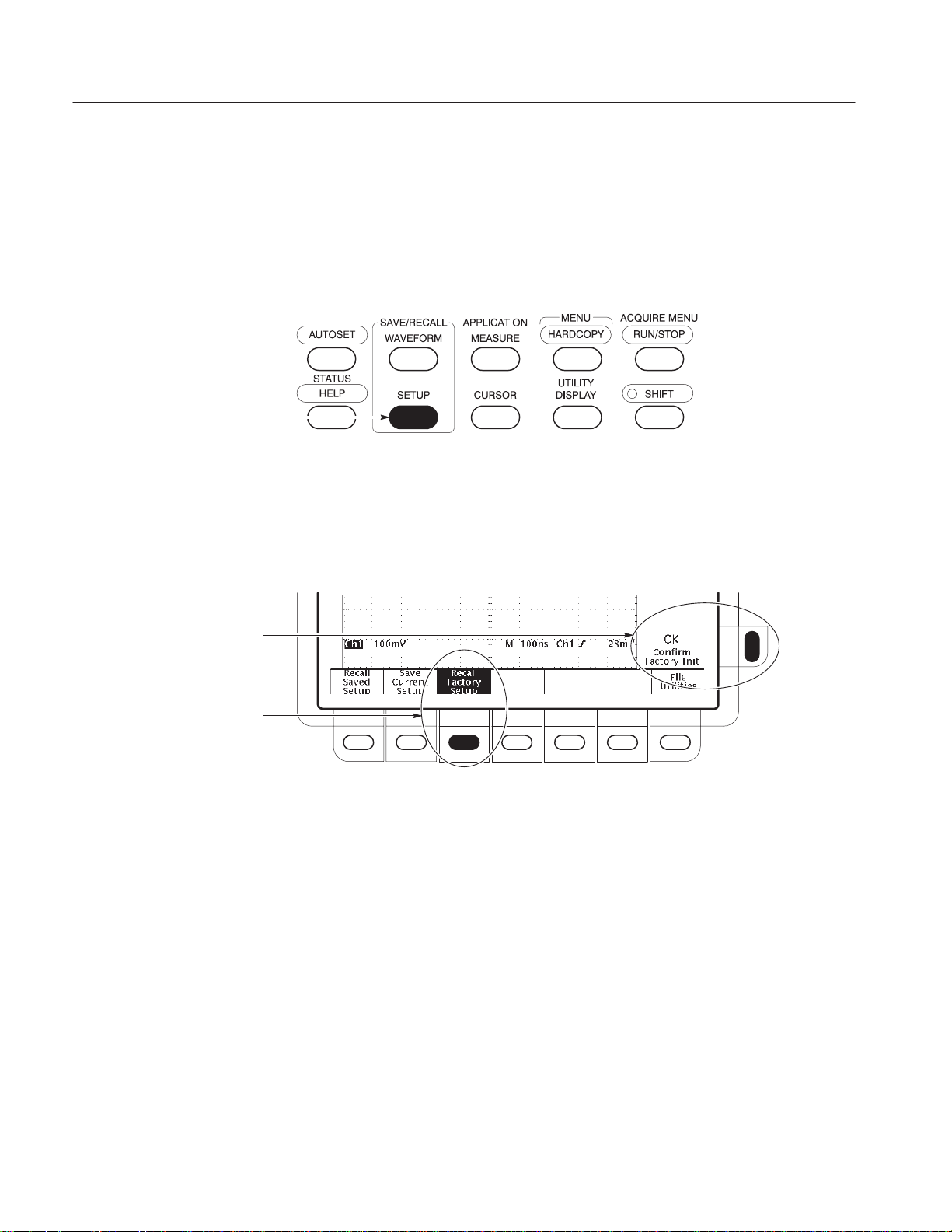
SETUP Button

Do the following steps to reset the digitizing oscilloscope to a known factory
default state. (Reset the oscilloscope anytime you begin a new task and need to
“start fresh” with known default settings.)

1. Press the save/recall SETUP button to display the Setup menu (see

Figure 2-2).

Figure 2-2: SETUP Button Location

The digitizing oscilloscope displays main menus along the bottom of the
screen. Figure 2-3 shows the Setup main menu.

OK Confirm Factory Init
Menu Item and Button

Recall Factory Setup

Menu Item and Button

Figure 2-3: The Displayed Setup Menu

2. Press the button directly below the Recall Factory Setup menu item.

The display shows side menus along the right side of the screen. The buttons
to select these side menu items are to the right of the side menu.

Because an accidental instrument reset could destroy a setup that took a long
time to create, the digitizing oscilloscope asks you to verify the Recall
Factory Setup selection (see Figure 2-3).

3. Press the button to the right of the OK Confirm Factory Init side menu

item.

2–12

TDS 420A, TDS 430A, TDS 460A & TDS 510A User Manual

Tutorial

NOTE. This manual uses the following notation to represent the sequence of
selections you made in steps 1, 2 and 3: Press save/recall SETUP

Factory Setup

(main) ➞ OK Confirm Factory Init (side).

➞ Recall

Note that a clock icon appears on screen. The oscilloscope displays this icon
when performing operations that take longer than several seconds.

4. Press SET LEVEL TO 50% (see Figure 2-4) to be sure the oscilloscope

triggers on the input signal.

Examine the Display

Elements

SET LEVEL TO 50% Button

Figure 2-4: SET LEVEL TO 50% Button

Read the following information to become familiar with the oscilloscope display.
Figure 2-5 shows the display that results from the oscilloscope reset. There are
several important points to observe:

H The trigger level bar shows that the waveform is triggered at a level near

50% of its amplitude (from step 4).

H The trigger position indicator shows that the trigger position of the

waveform is located at the horizontal center of the graticule.

H The channel reference indicator shows the vertical position of channel 1

with no input signal. This indicator points to the ground level for the channel
when its vertical offset is set to 0 V in the vertical menu; when vertical offset
is not set to 0 V, the indicator points to the vertical offset level.

H The trigger readout shows that the digitizing oscilloscope is triggering on

channel 1 (Ch1) on a rising edge and that the trigger level is about
200-300 mV.

H The time base readout shows that the main time base is set to a horizontal

scale of 500 ms/div.

TDS 420A, TDS 430A, TDS 460A & TDS 510A User Manual

2–13

Tutorial

H The channel readout indicates that channel 1 (Ch1) is displayed with DC

coupling. (In AC coupling, ~ appears after the volts/div readout.) The
digitizing oscilloscope always displays channel 1 at reset.

Right now, the channel, time base, and trigger readouts appear in the graticule
area because a menu is displayed. You can press the CLEAR MENU button at
any time to remove any menus and to move the readouts below the graticule.

Trigger Position

Indicator

Channel Ground

Reference Indicator

2–14

Channel
Readout

Time Base

Readout

Trigger

Readout

Figure 2-5: The Display After Factory Initialization

TDS 420A, TDS 430A, TDS 460A & TDS 510A User Manual

Example 1: Displaying a Waveform

The digitizing oscilloscope provides front panel knobs for you to adjust a
waveform, or it can automatically set up its controls to display a waveform. Do
the following tasks to learn how to adjust a waveform and how to autoset the
digitizing oscilloscope.

Tutorial

Adjusting the Waveform

Display

The display shows the probe compensation signal. It is a 1 kHz square wave of
approximately 0.5 V amplitude. Do the following steps to adjust the size and
placement of the waveform using the front-panel knobs.

Figure 2-6 shows the main VERTICAL and HORIZONTAL sections of the front
panel. Each has SCALE and POSITION knobs.

1. Turn the vertical SCALE knob clockwise. Observe the change in the

displayed waveform and the channel readout at the bottom of the display.

Figure 2-6: The VERTICAL and HORIZONTAL Controls

2. Turn the vertical POSITION knob first one direction, then the other.

Observe the change in the displayed waveform. Then return the waveform to
the center of the graticule.

TDS 420A, TDS 430A, TDS 460A & TDS 510A User Manual

2–15

Tutorial

3. Turn the horizontal SCALE knob one click clockwise. Observe the time

base readout at the bottom of the display. The time base should be set to
200 ms/div now, and you should see two complete waveform cycles on the
display.

Autoset the Oscilloscope

When you first connect a signal to a channel and display it, the signal displayed
may not be scaled and triggered correctly. Use the autoset function and you
should quickly get a meaningful display.

You should have a stable display of the probe compensation waveform from the
last step. Do the following steps to first create an unstable display and then to
automatically obtain a stable display:

1. To create an unstable display, slowly turn the trigger MAIN LEVEL knob

(see Figure 2-7) first one direction, then the other. Observe what happens
when you move the trigger level above the highest part of the displayed
waveform. Leave the trigger level in that untriggered state.

2. Press AUTOSET (see Figure 2-8) and observe the stable waveform display.

MAIN LEVEL Knob

2–16

Figure 2-7: TRIGGER Controls

AUTOSET Button

Figure 2-8: AUTOSET Button Location

Figure 2-9 shows the display after pressing AUTOSET. If necessary, you can
adjust the waveform using the knobs discussed earlier in this example.

TDS 420A, TDS 430A, TDS 460A & TDS 510A User Manual

Tutorial

Figure 2-9: The Display After Pressing Autoset

NOTE. If the corners on your displayed signal look rounded or pointed (see
Figure 2-10), then you may need to compensate your probe. See pages 3–83 and
3–89 for probe calibration and compensation procedures.

Figure 2-10: Display Signals Requiring Probe Compensation

TDS 420A, TDS 430A, TDS 460A & TDS 510A User Manual

2–17

Tutorial

Example 2: Displaying Multiple Waveforms

In this example you learn how to display and control more than one waveform at
a time.

Adding a Waveform

The VERTICAL section of the front panel contains the channel selection
buttons. On the TDS 420A, TDS 460A, and TDS 510A Digitizing Oscillo­scopes, they are CH 1, CH 2, CH 3, CH 4, and MORE (Figure 2-11). On the
TDS 430A, they are CH 1, CH 2, and MORE.

Figure 2-11: The Channel Buttons and Lights

2–18

Each of the channel (CH) buttons has a light above or beside its label. Do the
following steps to add a waveform to the display:

1. If you are not continuing from the previous example, follow the instructions

on page 2–11 under the heading Setting Up for the Examples.

2. Press SETUP
Init

(side).

3. Press AUTOSET.

4. Press CH 2.

The display shows a second waveform, which represents the signal on
channel 2.

➞ Recall Factory Setup (main) ➞ OK Confirm Factory

TDS 420A, TDS 430A, TDS 460A & TDS 510A User Manual

There are several other things to observe:
H The channel readout on the display now shows the settings for both Ch1

and Ch2.

H There are two channel indicators at the left edge of the graticule. Right

now, they overlap.

H The light by the CH 2 button is now on, and the vertical controls are

now set to adjust channel 2.

H The trigger source is not changed by adding a channel. (You can change

the trigger source by using the TRIGGER MENU.)

5. Turn the vertical POSITION knob clockwise to move the channel 2

waveform up on the graticule. Notice that the channel reference indicator for
channel 2 moves with the waveform.

Tutorial

6. Press VERTICAL MENU

➞ Coupling (main).

The vertical menu gives you control over many vertical channel parameters
(Figure 2-12). Although there can be more than one channel displayed, the
vertical menu and buttons only adjust the selected channel.

Each menu item in the Vertical menu displays a side menu. Right now, the
Coupling item in the main menu is highlighted, which means that the side
menu shows the coupling choices.

7. Press W

(side) to toggle the selection to 50 W; this changes the input

coupling of channel 2 from 1 MW to 50 W. The channel readout for
channel 2 (near the bottom of the graticule) now shows an W indicator.

TDS 420A, TDS 430A, TDS 460A & TDS 510A User Manual

2–19

Tutorial

Ch2 Reference Indicator

Side Menu Title

Assign Controls to

Another Channel

Figure 2-12: The Vertical Main Menu and Coupling Side Menu

Pressing a channel (CH) button sets the vertical controls to that channel. It also
adds the channel to the display if that waveform is not already displayed. To
explore assigning controls to different channels, do the following steps:

1. Press CH 1.
Observe that the side menu title shows Ch1 (see Figure 2-13) and that the

indicator next to CH 1 is on. Note the highlighted menu item in the side
menu also changes from the 50 W channel 2 setting to the 1 MW impedance
setting of channel 1.

2. Press CH 2

➞ W (side) to toggle the selection to 1MW. This returns the

coupling impedance of channel 2 to its initial state.

2–20

TDS 420A, TDS 430A, TDS 460A & TDS 510A User Manual

Side Menu Title

Tutorial

Remove a Waveform

Figure 2-13: The Menus After Changing Channels

Pressing the WAVEFORM OFF button removes the waveform for the currently
selected channel. If the waveform you want to remove is not already selected,
select that channel using the channel (CH) button. To remove a waveform from
the display, do the following steps:

1. Press WAVEFORM OFF (under the vertical SCALE knob).

Since the CH 2 light was on when you pressed the WAVEFORM OFF
button, the channel 2 waveform was removed.

The channel (CH) lights now indicate channel 1. Channel 1 has become the
selected channel. When you remove the last waveform, all the CH lights are
turned off.

2. Press WAVEFORM OFF again to remove the channel 1 waveform.

TDS 420A, TDS 430A, TDS 460A & TDS 510A User Manual

2–21

Tutorial

Example 3: Taking Automated Measurements

The digitizing oscilloscope can measure many waveform parameters automati­cally and read out the results on screen. Do the following tasks to discover how
to set up the oscilloscope to measure waveforms automatically.

Display Measurements

Automatically

To take automated measurements, do the following steps:

1. If you are not continuing from the previous example, follow the instructions
on page 2–11 under the heading “Setting Up for the Examples.”

2. Press SETUP
Init

(side).

3. Press AUTOSET.

4. Press MEASURE to display the Measure main menu (see Figure 2-14).

➞ Recall Factory Setup (main) ➞ OK Confirm Factory

2–22

Figure 2-14: Measure Main Menu and Select Measurement Side Menu

5. If it is not already selected, press Select Measrmnt
that menu item indicates which channel the measurement will be taken from.
All automated measurements are made on the selected channel.

TDS 420A, TDS 430A, TDS 460A & TDS 510A User Manual

(main). The readout for

Tutorial

The Select Measurement side menu lists the measurements that can be taken.
Up to four can be taken and displayed at any one time. Pressing the button
next to the –more– menu item displays the other measurement selections.

6. Press Frequency

–more–

(side) repeatedly until the Frequency item appears, then press

Frequency

(side). If the Frequency menu item is not visible, press

(side).

Observe that the frequency measurement appears within the right side of the
graticule area. The measurement readout includes the notation Ch1, meaning
that the measurement is taken on the channel 1 waveform. (To take a
measurement on another channel, select that channel, and then select the
measurement.)

7. Press Positive Width
Positive Duty Cycle

(side) ➞ –more– (side) ➞ Rise Time (side) ➞

(side).

All four measurements are displayed.

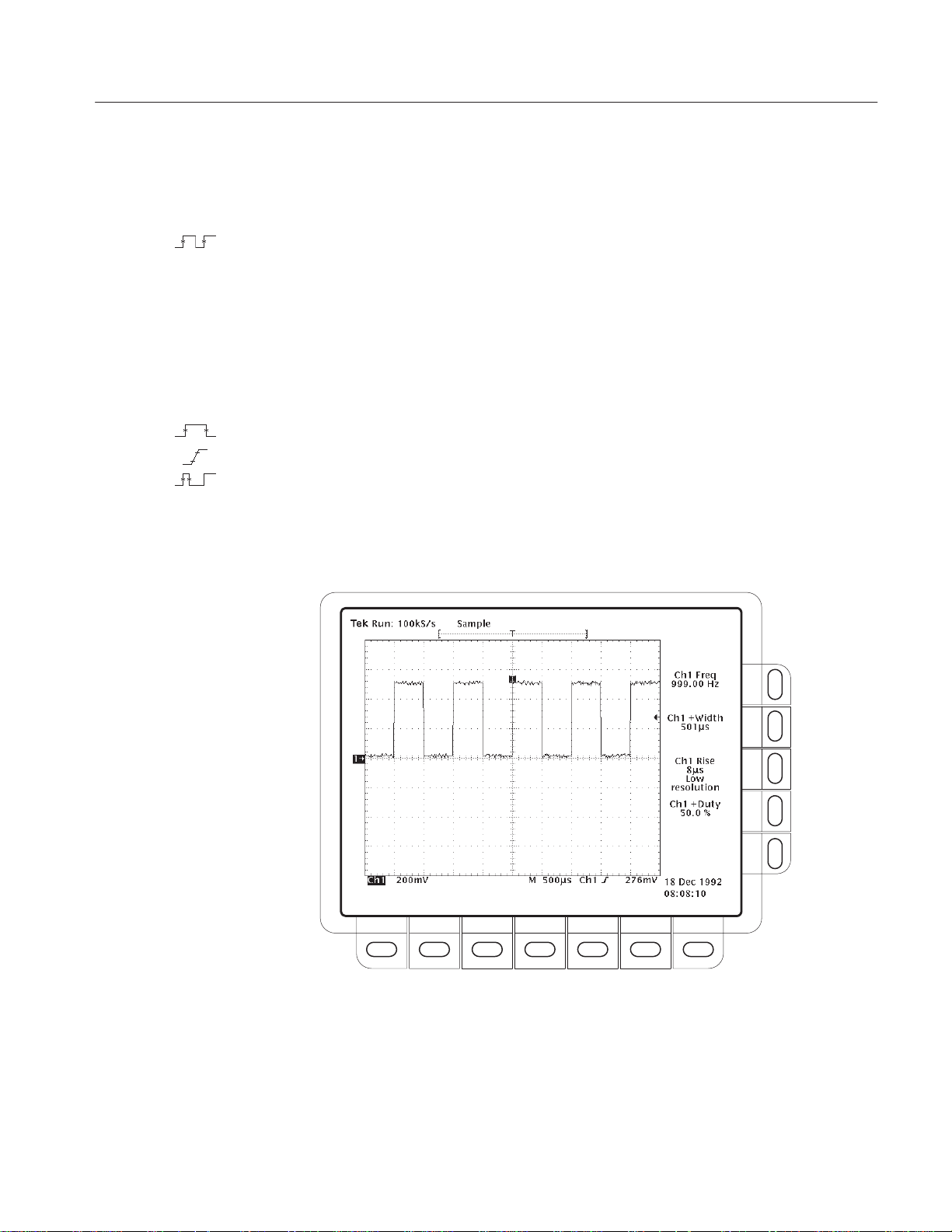
8. To move the measurement readouts outside the graticule area, press CLEAR
MENU (see Figure 2-15).

Figure 2-15: Four Simultaneous Measurement Readouts

TDS 420A, TDS 430A, TDS 460A & TDS 510A User Manual

2–23

Tutorial

Remove Measurement

Readouts

Examine the Measurement

Reference Levels

General Purpose Knob

Setting and Readout

General Purpose

Knob Icon

To remove measurements you no longer want displayed:
Press MEASURE

ment 2, and Measurement 4

➞ Remove Measrmnt (main) ➞ Measurement 1, Measure-

(side) to remove those measurements. Leave the

rise time measurement displayed.

To examine the current values:

Press Reference Levels

(main) ➞ High Ref (side).

Highlighted Menu Item with Boxed

Readout Value

Change the Measurement

Reference Levels

Figure 2-16: General Purpose Knob Indicators

By default, the measurement system uses the 10% and 90% levels of the
waveform for taking the rise time measurement. You can change these values to
other percentages or change them to absolute voltage levels.

To examine the current values, press Reference Levels

(main) ➞ High Ref

(side).
The general purpose knob is now set to adjust the high reference level (Fig-

ure 2-16).

2–24

TDS 420A, TDS 430A, TDS 460A & TDS 510A User Manual

Tutorial

There are several important things to observe on the screen:
H The knob icon appears at the top of the screen. The knob icon indicates that

the general purpose knob is set to adjust a parameter.

H The upper right corner of the screen shows the readout High Ref: 90%.
H The High Ref side menu item is highlighted, and a box appears around the

90% readout in the High Ref menu item. The box indicates that the general
purpose knob is currently set to adjust that parameter.

To adjust the high level to 80%, turn the general purpose knob.

Display a Snapshot of

Automated Measurements

You can pop up a display of almost all of the automated measurements. To
display a snapshot of automated measurements of the selected channel, do the
following steps:

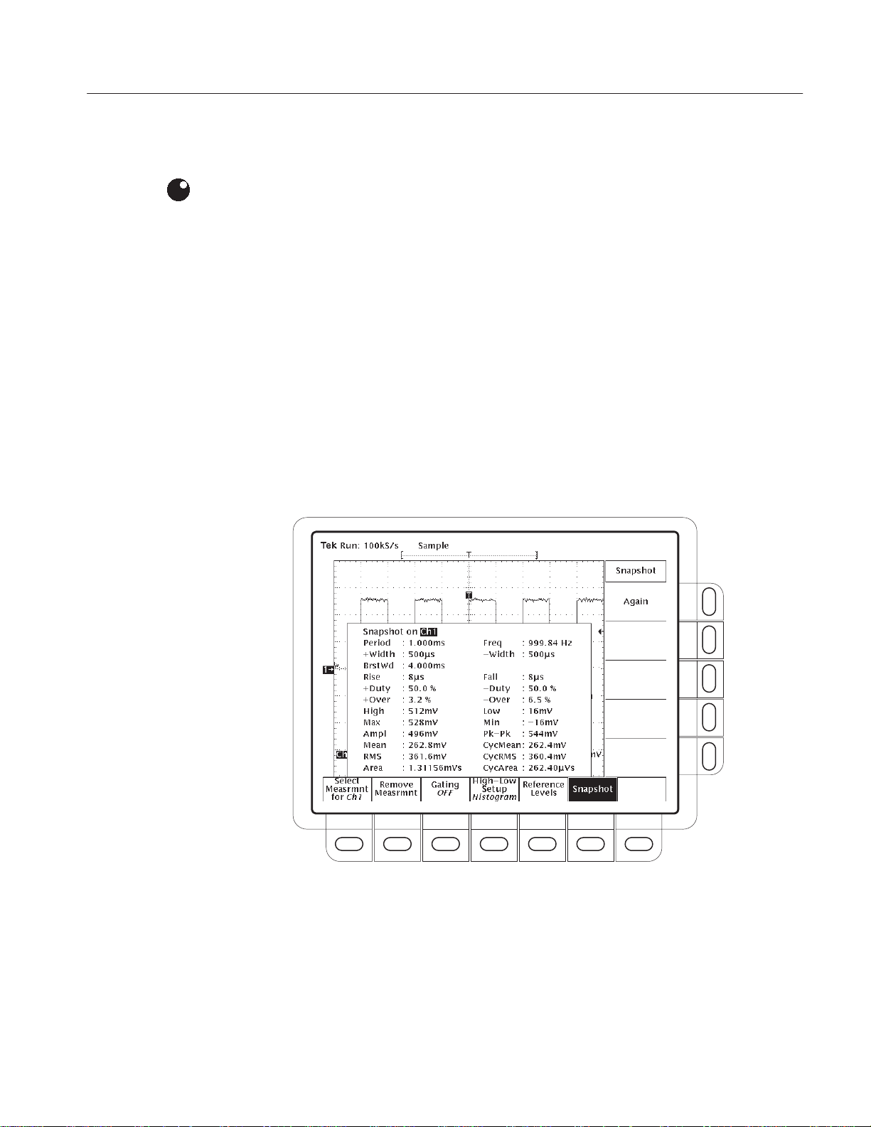
1. Press Snapshot
waveform measurements. (See Figure 2-17).

(main) to pop up a snapshot of all available single

Figure 2-17: Snapshot of Channel 1

TDS 420A, TDS 430A, TDS 460A & TDS 510A User Manual

2–25

Tutorial

Example 4: Saving Setups

The digitizing oscilloscope can save its control settings and recall them later to
quickly re-establish the previously saved state. Do the following tasks to learn
how to save, and then recall, a setup.

Save a Setup

First, you need to create an instrument setup you want to save. Perform the
following steps to create and save a setup that is complex enough that you might
prefer not to go through all these steps each time you want that display:

1. If you are not continuing from the previous example, follow the instructions

on page 2–11 under the heading Setting Up for the Examples.

2. Press SETUP
Init

(side).

3. Press

4. Press MEASURE

5. Press CH 2

To save the setup, do the following steps:

6. Press SETUP

➞ AUTOSET.

the –more– side menu item if the Frequency selection does not appear in
the side menu.)

menu (see Figure 2-18).

➞ Recall Factory Setup (main) ➞ OK Confirm Factory

➞ Select Measrmnt (main) ➞ Frequency (side). (Press

➞ CLEAR MENU.

➞ Save Current Setup (main) to display the Setup main

2–26

TDS 420A, TDS 430A, TDS 460A & TDS 510A User Manual

Tutorial

Recall a Setup

Figure 2-18: Save/Recall Setup Menu

7. Press one of the To Setup side menu buttons to store the current instrument

settings into that setup location. Remember which setup location you
selected for use later.

Once you have saved a particular setup, you can change the settings as you wish,
knowing that you can come back to that setup at any time.

8. Press MEASURE

➞ Positive Width (side) to add that measurement to the

display.

To recall the setup, press SETUP

(side) for the setup location you used in the last exercise.

Setup

➞ Recall Saved Setup (main) ➞ Recall

TDS 420A, TDS 430A, TDS 460A & TDS 510A User Manual

2–27

Tutorial

2–28

TDS 420A, TDS 430A, TDS 460A & TDS 510A User Manual

Overview

This chapter describes the details of operating the digitizing oscilloscope. It
contains an alphabetical list of tasks you can perform with the digitizing
oscilloscope. Use this chapter to answer specific questions about instrument
operation. The following tasks are included:

H Accessing Help H Remote Communication
H Acquisition Modes H Roll Mode
H Delayed Triggering H Saving and Recalling Setups
H Determining Status H Saving and Recalling Waveforms
H Display Modes H Selecting Channels
H Edge Triggering H Setting up Automatically
H Fast Fourier Transforms H Signal Path Compensation
H File System H Taking Cursor Measurements
H Hardcopy H Vertical Control
H Horizontal Control H Video Triggering
H Limit Testing H Waveform Differentiation
H Measuring Waveforms H Waveform Integration
H Probe Cal H Waveform Math
H Probe Compensation H Zoom
H Pulse Triggering

Many of these tasks list steps you perform to accomplish the task. You should
read Conventions on page x of Preface before reading about these tasks.

TDS 420A, TDS 430A, TDS 460A & TDS 510A User Manual

3–1

Overview

3–2

TDS 420A, TDS 430A, TDS 460A & TDS 510A User Manual

Accessing Help

The on-line help system provides brief information about each of the digitizing
oscilloscope controls.

To use the on-line help system:
Press HELP to display information on any front panel button, knob, or menu

item (see Figure 3-1).
Press HELP again to return to the regular operating mode. Whenever the

oscilloscope is in help mode, pressing any button (except HELP or SHIFT),
turning any knob, or pressing any menu item displays help text on the screen that
discusses that control.

On-line help is available for each menu selection displayed at the time the HELP
button is first pressed. If you are in help mode and want to see help on selections
from non-displayed menus, you first exit help mode, display the menu you want
information on, and press HELP again to re-enter help mode.

Figure 3-1: Initial Help Screen

TDS 420A, TDS 430A, TDS 460A & TDS 510A User Manual

3–3

Accessing Help

3–4

TDS 420A, TDS 430A, TDS 460A & TDS 510A User Manual

Acquisition Modes

The acquisition system has several options for converting analog data into digital
form. The Acquisition menu lets you determine the acquisition mode, whether or
not to permit equivalent time sampling, and how to start and stop acquisitions.

Description of Modes

The digitizing oscilloscope supports five acquisition modes:

H Sample
H Peak Detect
H Hi Res
H Envelope
H Average

The Sample, Peak Detect, and Hi Res modes operate in real-time on a single
trigger event, provided the digitizing oscilloscope can acquire enough samples
for each trigger event. Envelope and Average modes operate on multiple
acquisitions. The digitizing oscilloscope averages or envelopes several wave­forms on a point-by-point basis.

Sample Mode

Peak Detect Mode

Hi Res Mode

TDS 420A, TDS 430A, TDS 460A & TDS 510A User Manual

In Sample mode, the oscilloscope creates a record point by saving the first
sample (of perhaps many) during each acquisition interval. (An acquisition
interval is the time covered by the waveform record divided by the record
length.) This is the default mode.

Peak Detect mode alternates between saving the highest sample in one acquisi­tion interval and lowest sample in the next acquisition interval. This mode only
works with real-time, non-interpolated sampling.

If you set the time base so fast that it requires real-time interpolation or
equivalent-time sampling, the mode automatically changes from Peak Detect to
Sample, although the menu selection does not change.

In Hi Res mode, the digitizing oscilloscope averages all samples taken during an
acquisition interval to create a record point. That average results in a higher-reso­lution, lower-bandwidth waveform.

3–5

Acquisition Modes

NOTE. In Hi Res mode the frequency of the external clock signal (TDS 460A,
TDS 430A, and TDS 420A only) must be less than or equal to the frequency set
in the external clock menu. If the frequency of the external clock signal is greater
than the frequency in the menu, the displayed waveform will have the wrong
amplitude.

This mode only works with real-time, non-interpolated sampling. If you set the
time base so fast that it requires real-time interpolation or equivalent-time
sampling, the mode automatically becomes Sample, although the menu selection
does not change.

A key advantage of Hi Res is its potential for increasing resolution regardless of
the input signal. Tables 3–1 and 3–2 illustrate how you can obtain up to
15 significant bits with Hi Res mode. Note that resolutions above 15 bits are not
allowed. The bits of resolution shown in the tables are theoretically achievable.
Actual resolution may vary as a function of the correlated noise sources in the
test environment.

T able 3–1: TDS 460A, TDS 430A, and TDS 420A Resolution
Bits

Time Base Speed Bits of Resolution

1 ms and faster 8 bits
2 ms to 5 ms 9 bits
10 ms to 20 ms 10 bits
50 ms to 100 ms 11 bits
200 ms to 500 ms 12 bits

T able 3–2: TDS 510A Resolution Bits

Time Base Speed Bits of Resolution

400 ns and faster 8 bits
1 ms to 2 ms 9 bits
5 ms to 10 ms 10 bits
20 ms to 50 ms 11 bits
50 ms to 100 ms 11 bits
100 ms to 200 ms 12 bits
500 ms 13 bits
1 ms to 2 ms 14 bits
5 ms and slower 15 bits

3–6

TDS 420A, TDS 430A, TDS 460A & TDS 510A User Manual

Acquisition Modes

Envelope Mode

Average Mode

Envelope mode lets you acquire and display a waveform record that shows the
extremes in variation over several acquisitions. You specify the number of
acquisitions over which to accumulate the data. The oscilloscope saves the
highest and lowest values in two adjacent intervals similar to the Peak Detect
mode. But Envelope mode, unlike Peak Detect, gathers peaks over many trigger
events.

The final display shows the most extreme values for all the acquisitions for each
point in the waveform record.

NOTE. Envelope and Average acquisition modes disable Roll mode. See Roll
Mode beginning on page 3–99.

Average mode lets you acquire and display a waveform record that is the
averaged result of several acquisitions. This mode reduces random noise. The
oscilloscope acquires data after each trigger event using Sample mode.

Checking the Acquisition Readout

To determine the acquisition sampling rate, the acquisition state (running or
stopped), and the acquisition mode, check the acquisition readout at the top of
the display (see Figure 3-2). The “running” state shows the sample rate (or
External Clock when external clock is enabled) and acquisition mode. The
“stopped” state shows the number of acquisitions acquired since the last stop or
major change.

TDS 420A, TDS 430A, TDS 460A & TDS 510A User Manual

3–7

Acquisition Modes

Acquisition Readout

Figure 3-2: Acquisition Menu and Readout

Selecting an Acquisition Mode

The oscilloscope provides several acquisition modes. To bring up the acquisition
menu (Figure 3-2) and choose how the digitizing oscilloscope creates points in
the waveform record:

Press SHIFT ACQUIRE MENU
Res, Envelope, or Average

NOTE. With some longer record lengths, the digitizing oscilloscope will not
allow selecting Hi Res mode or will reduce the record length setting.

When you select Envelope or Average, you can enter the number of waveform
records to be enveloped or averaged using the general purpose knob.

Selecting Repetitive Sampling

To limit the digitizing oscilloscope to real-time sampling or let it choose between
real-time or equivalent-time sampling:

➞ Mode (main) ➞ Sample, Peak Detect, Hi

(side).

3–8

Press SHIFT ACQUIRE MENU
(side).

TDS 420A, TDS 430A, TDS 460A & TDS 510A User Manual

➞ Repetitive Signal (main) ➞ ON or OFF

To Stop After

Acquisition Modes

ON (Enable ET) uses both the real time and the equivalent time features of the
digitizing oscilloscope.

OFF (Real Time Only) limits the digitizing oscilloscope to real time sampling. If
the digitizing oscilloscope cannot accurately get enough samples for a complete
waveform, the oscilloscope uses the interpolation method selected in the display
menu to fill in the missing record points.

To choose the event that signals the oscilloscope to stop acquiring waveforms,
do the following step:

Press SHIFT ACQUIRE MENU
only, Single Acquisition Sequence, or Limit Test Condition Met
Figure 3-3).

➞ Stop After (main) ➞ RUN/STOP button

(side) (see

Figure 3-3: Acquire Menu — Stop After

RUN/STOP button only

RUN/STOP button. Pressing the RUN/STOP button once stops the acquisitions.
The upper left hand corner in the display indicates Stopped and shows the
number of acquisitions. If you press the button again, the digitizing oscilloscope
resumes taking acquisitions.

TDS 420A, TDS 430A, TDS 460A & TDS 510A User Manual

(side) lets you start or stop acquisitions by toggling the

3–9

Acquisition Modes

Single Acquisition Sequence (side) lets you run a single sequence of acquisitions
by pressing the RUN/STOP button.

In Envelope or Average mode, the digitizing oscilloscope makes the specified
number of acquisitions to complete the averaging or enveloping task.

If the oscilloscope is in equivalent-time mode and you press Single Acquisition
Sequence

(side), it continues to recognize trigger events and acquire samples

until the waveform record is filled.

NOTE. To quickly select Single Acquisition Sequence without displaying the
Acquire and Stop After menus, press SHIFT FORCE TRIG. (You still must
display the Acquire menu and then the Stop After menu to leave Single Acquisi­tion Sequence operation.)

Limit Test Condition Met (side) lets you acquire waveforms until waveform data

exceeds the limits specified in the limit test. Then acquisition stops. At that
point, you can also specify other actions for the oscilloscope to take using the
selections available in the Limit Test Setup main menu.

NOTE. In order for the digitizing oscilloscope to stop acquisition when limit test
conditions are met, limit testing must be turned ON, using the Limit Test Setup
main menu.

Setting up limit testing requires several more steps. See Limit Testing, on
page 3–63.

3–10

TDS 420A, TDS 430A, TDS 460A & TDS 510A User Manual

Delayed Triggering

The digitizing oscilloscope provides a main time base and a delayed time base.
The delayed time base, like the main time base, requires a trigger signal and an
input source dedicated to that signal. You can only use delay with the edge
trigger and certain classes of main pulse triggers. This section describes how to
delay the acquisition of waveforms.

There are two different ways to delay the acquisition of waveforms: delayed runs
after main and delayed triggerable. Only delayed triggerable uses the delayed
trigger system.

Delayed runs after main looks for a main trigger, then waits a user-defined time,
and then starts acquiring (see Figure 3-4).

Wait for

Main

Trigger

Wait User-specified

Time

Acquire

Data

Figure 3-4: Delayed Runs After Main

Delayed triggerable looks for a main trigger and then, depending on the type of
delayed trigger selected, makes one of the types of delayed triggerable mode
acquisitions listed below (see Figure 3-5).

Wait for

Main

Trigger

Wait User-specified Time,

Number of Delayed

Trigger Events or Number

of External Clocks

Wait for Delay
Trigger Event

Acquire

Data

Figure 3-5: Delayed Triggerable

After Time waits the user-specified time, then waits for the next delayed trigger
event, and then acquires.

After Events waits for the specified number of delayed trigger events and
then acquires.

After Events/Time (TDS 510A only) waits for the specified number of delayed
trigger events, then waits the user-specified time, and then acquires.

External clks (TDS 400A) waits for the specified number of external clocks and
then acquires.

TDS 420A, TDS 430A, TDS 460A & TDS 510A User Manual

3–11

Delayed Triggering

To Run After Delay

NOTE. When using the delayed triggerable mode, the digitizing oscilloscope
provides a conventional edge trigger for the delayed time base. The delayed time
base will not trigger if the main trigger type (as defined in the Main Trigger
menu) is logic, or if the main trigger type is pulse with the runt trigger class
selected.

You use the Horizontal menu to select and define either delayed runs after main
or delayed triggerable. Delayed triggerable, however, requires further selections
in the Delayed Trigger menu. Do the following steps to set the delayed time base
to run immediately after delay:

To Trigger After Delay

1. Press HORIZONTAL MENU
(side)

➞ Delayed Runs After Main (side).

2. Use the general purpose knob to set the delay time.

If you press Intensified
timebase record that shows where the delayed timebase record occurs relative to
the main trigger. For Delayed Runs After Main mode, the start of the intensified
zone corresponds to the start of the delayed timebase record. The end of the zone
corresponds to the end of the delayed record.

To learn how to set the intensity level, see Display Modes on page 3–17.

The Main Trigger menu settings must be compatible with Delayed Triggerable.
To select Delayed Triggerable mode, do the following steps:

1. Press TRIGGER MENU.

2. Press Type

3. Press HORIZONTAL MENU

(side)

(main) and either Edge or Pulse as fits your application.

➞ Delayed Triggerable (side).

(side), you display an intensified zone on the main

➞ Time Base (main) ➞ Delayed Only

➞ Time Base (main) ➞ Delayed Only

3–12

NOTE. The Delayed Triggerable menu item is not selectable unless incompatible
Main Trigger menu settings are eliminated. If such is the case, the Delayed
Triggerable menu item is dimmer than other items in the menu.

TDS 420A, TDS 430A, TDS 460A & TDS 510A User Manual

Delayed Triggering

By pressing Intensified (side), you can display an intensified zone that shows
where the delayed timebase record may occur (a valid delay trigger event
must be received) relative to the main trigger on the main timebase. For
Delayed Triggerable After mode, the start of the intensified zone corresponds
to the possible start point of the delayed timebase record. The end of the
zone continues to the end of main timebase, since a delayed time base record
may be triggered at any point after the delay time elapses.

To learn how to define the intensity level of the normal and intensified
waveform, see Display Modes on page 3–17.

Now you need to bring up the Delayed Trigger menu so you can define the
delayed trigger event.

4. On a TDS 400A, press SHIFT DELAYED TRIG
Triggerable After Time, Events, or Ext clks

5. On the TDS 510A, press SHIFT DELAYED TRIG
Triggerable After Time, Events, or Events/Time

➞ Delay by (main) ➞

(side) (Figure 3-6).

➞ Delay by (main) ➞

(side).

6. Enter the delay time or events using the general purpose knob or the keypad.
Hint: You can go directly to the Delayed Trigger menu (see steps 4 and 5).

By selecting either Triggerable After Time, Events, or Events/Time, the
oscilloscope automatically switches to Delayed Triggerable in the Horizontal
menu. If you wish to leave Delayed Triggerable, you still need to display the
Horizontal menu.

The Source menu lets you select which input is the delayed trigger source.

7. Press Source

(main) ➞ Ch1, Ch2, Ch3, Ch4, DC Aux, or Auxiliary (side).

TDS 420A, TDS 430A, TDS 460A & TDS 510A User Manual

3–13

Delayed Triggering

Figure 3-6: Delayed Trigger Menu (TDS 400A shown)

8. To define how the input signal is coupled to the delayed trigger, press
Coupling

(main) ➞ DC, AC, HF Rej, LF Rej, or Noise Rej (side). For

descriptions of these coupling types, see To Specify Coupling on page 3–23.

9. To select the slope that the delayed trigger occurs on, press Slope (main).
Choose between the rising edge and falling edge slopes.

When using Delayed Triggerable mode to acquire waveforms, two trigger
bars are displayed. One trigger bar indicates the level set by the main trigger
system; the other indicates the level set by the delayed trigger system.

10. Press Level

(main) ➞ Level, Set to TTL, Set to ECL, or Set to 50% (side).

For a description of these level settings, see To Set Level on page 3–24.

3–14

TDS 420A, TDS 430A, TDS 460A & TDS 510A User Manual

Determining Status

The Status menu lets you see information about the oscilloscope state.

To Display the Status

To display the Status menu (see Figure 3-7):

Firmware Date

Press SHIFT STATUS
I/O

(side).

System displays information about the firmware, Horizontal, Zoom, Acquisition,
Limit Test, Measure, and Hardcopy (TDS 510A) systems.

Display displays information about the display system.
Trigger displays information about the triggers.
Waveforms displays information about the various waveforms, including live,

math, and reference.
I/O displays information about the I/O port(s).

➞ Status (main) ➞ System, Trigger, Waveforms, or

Figure 3-7: Status Menu — System (TDS 400A shown)

TDS 420A, TDS 430A, TDS 460A & TDS 510A User Manual

3–15

Determining Status

To Display the Banner

To display the banner (firmware version, options, and copyright):
Press SHIFT STATUS

➞ Banner (main). (See Figure 3-8.)

Figure 3-8: Banner Display

3–16

TDS 420A, TDS 430A, TDS 460A & TDS 510A User Manual

Display Modes

This section describes how to adjust the oscilloscope display style, intensity
level, graticule, and format.

Change Display Settings

To bring up the Display menu, press DISPLAY.

Select the Display Style

Press DISPLAY
Infinite Persistence, or Variable Persistence

➞ Style (main) ➞ Vectors, Intensified Samples, Dots,

(side) (Figure 3-9).

Figure 3-9: Display Menu — Style

Vectors style displays draw vectors (lines) between the record points.
Dots style displays waveform record points as dots.
Intensified Samples style also displays waveform record points as dots. However,

the points actually sampled are displayed intensified relative to the interpolated
points.

TDS 420A, TDS 430A, TDS 460A & TDS 510A User Manual

3–17

Display Modes

In addition to choosing Intensified Samples in the side menu, the oscilloscope
must be interpolating (equivalent time must be off) or Zoom must be on with its
horizontal expansion greater that 1X. See Zoom beginning on page 3–143.

Variable Persistence accumulates the record points on screen over many acquisi-

tions and displays them only for a specific time interval. In that mode, the
display behaves like that of an analog oscilloscope.

Infinite Persistence accumulates the record points until you change some control
(such as scale factor) causing the display to be erased.

Adjust Intensity

Set Display Readout

Options

Intensity lets you set overall, text/graticule, and waveform intensity (brightness)
levels. To set the intensity:

Press DISPLAY

Contrast

(side). Enter the intensity percentage values with the general purpose

➞ Intensity (main) ➞ Overall, Text/Grat, Waveform, or

knob or keypad.

NOTE. The Intensified setting for Timebase in the horizontal menu causes a zone
on the waveform to be intensified relative to the rest of the waveform. If the
contrast is set to 100%, you can not distinguish the intensified portion from the
rest of the waveform because both are the same brightness.

To control whether the trigger indicator, trigger level bar, and current date and
time appear on the display and what style trigger level bar, long or short, is
displayed:

1. Press DISPLAY

➞ Readout (main).

2. To select whether or not to display a ‘T’ indicating the trigger point, Toggle
Display ‘T’ @ Trigger Point

(side). You can select ON or OFF. (The

trigger point indicates the position of the trigger in the waveform record.)

3–18

3. To select either the short or the long trigger bar or to turn the trigger bar off,
toggle Trigger Bar Style

(side). (See Figure 3-10. Note that both styles are

shown for illustrating purposes, but you can only display one style at a time.)
The trigger bar is only displayed if the trigger source is an active, displayed

waveform. Also, two trigger bars are displayed when delay triggerable
acquisitions are displayed . The trigger bar is a visual indicator of the trigger
level.

4. Press Display Date/Time

(side) to turn it on or off. Push Clear Menu to see

the current date and time. See To Date/Time Stamp Your Hardcopy on
page 3–49 for more information.

TDS 420A, TDS 430A, TDS 460A & TDS 510A User Manual

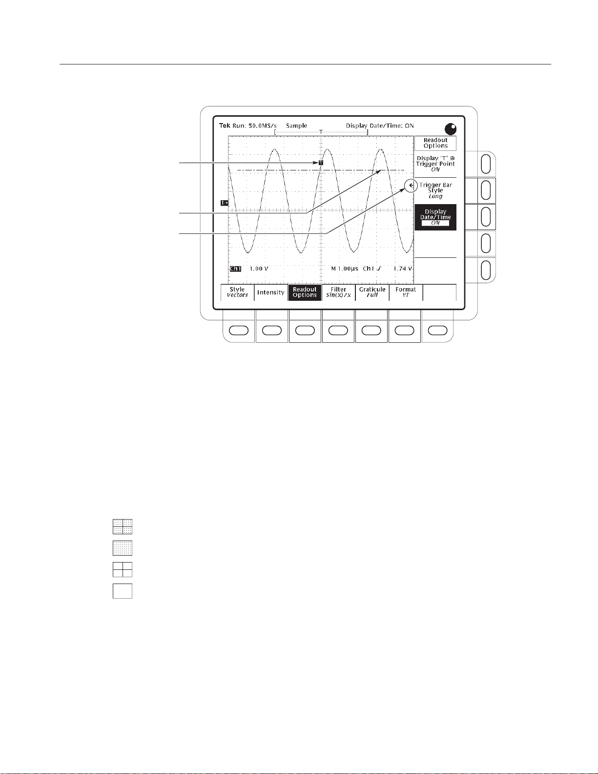
Trigger Point Indicator

Trigger Bar—Long Style

-or-

Trigger Bar—Short Style

Display Modes

Select Interpolation Filter

Select the Graticule Type

Figure 3-10: Trigger Point and Level Indicators

To select the display filter type (sin(x)/x interpolation and linear interpolation):
Press DISPLAY

polation

(side).

➞ Filter (main) ➞ Sin(x)/x Interpolation or Linear Inter-

To select the graticule type:
Press DISPLAY

or PAL

(side).

➞ Graticule (main) ➞ Full, Grid, Cross Hair, Frame, NTSC

Full provides a grid, cross hairs, and a frame.
Grid displays a frame and a grid.
Cross Hair provides cross hairs and a frame.
Frame displays just a frame.
NTSC provides a grid useful for measuring NTSC-class waveforms.
PAL provides a grid useful for measuring PAL-class waveforms.

TDS 420A, TDS 430A, TDS 460A & TDS 510A User Manual

3–19

Display Modes

NOTE. Selecting either NTSC or PAL graticule automatically changes the
vertical scale, position settings, coupling, and sets to zero any vertical offset of
any channel displayed. These settings are not restored after switching to other
graticule types.

Select the Display Format

There are two display formats: YT and XY.
YT is the conventional oscilloscope display format. It shows a signal voltage (the

vertical axis) as it varies over time (the horizontal axis).
XY format compares the voltage levels of two waveform records point by point.

That is, the digitizing oscilloscope displays a graph of the voltage of one
waveform record against the voltage of another waveform record. This mode is
particularly useful for studying phase relationships.

To set the display axis format:
Press DISPLAY

➞ Format (main) ➞ XY or YT (side).

When you choose the XY mode, the input you have selected is assigned to the
X-axis and the digitizing oscilloscope automatically chooses the Y-axis input
(see Table 3–3).

T able 3–3: XY Format Pairs

X-Axis Channel (User Selectable) Y -Axis Channel (Fixed)

Ch 1 Ch 2
Ch 3 (TDS 420A, TDS 460A, and TDS 510A

only)

Ch 4 (TDS 420A, TDS 460A, and TDS 510A
only)

3–20

If you press the WAVEFORM OFF button for an XY channel, the digitizing
oscilloscope deletes the XY graph of of the channels.

Since selecting YT or XY affects only the display, the horizontal and vertical
scale and position knobs and menus control the same parameters regardless of
the mode selected. Specifically, in XY mode, the horizontal scale continues to
control the time base and the horizontal position continues to control which
portion of the waveforms are displayed.

XY format is a dot-only display, although it can have persistence. The Vector
style selection has no effect when you select XY format.

You cannot display Math waveforms in XY format. They disappear from the
display when you select XY.

TDS 420A, TDS 430A, TDS 460A & TDS 510A User Manual

Edge Triggering

An edge trigger event occurs when the trigger source passes through a specified
voltage level (the trigger level) in a specified direction (the trigger slope). You
will likely use edge triggering for most of your measurements. This section
describes how to use edge triggering. It also explains how to select the trigger
mode, auto or normal, for all trigger types.

To Check Edge Trigger Status

To quickly check if edge triggers are selected, check the Trigger readout. When
edge triggers are selected, the trigger readout displays the trigger source, as well
as the trigger slope and level (see Figure 3-11).

Main Time Base Time/Div

Main Time Base

Figure 3-11: Edge Trigger Readouts

To determine the trigger status, check the TRIG’D, READY, and ARM status
lights in the Trigger control area (see Figure 3–26):

H When TRIG’D is lighted, the digitizing oscilloscope has recognized a valid

trigger and is filling the posttrigger portion of the waveform.

H When READY is lighted, the digitizing oscilloscope can accept a valid

trigger event and it is waiting for that event to occur.

Main Trigger

Source = Ch 1

Main Trigger
Slope = Rising Edge

Main Trigger Level

H When ARM is lighted, the trigger circuitry is filling the pretrigger portion of

the waveform record.

TDS 420A, TDS 430A, TDS 460A & TDS 510A User Manual

3–21

Edge Triggering

Trigger Position Relative to the

Display and Waveform Record.

H When both TRIG’D and READY are lighted, the digitizing oscilloscope has

recognized a valid main trigger and is waiting for a delayed trigger. When it
recognizes a delayed trigger it will fill in the posttrigger portion of the
delayed waveform.

H When ARM, TRIG’D, and READY are all off, the digitizer is stopped.
To determine where the trigger point is located in the waveform record and with

respect to the display, check the record view at the top of the display (see
Figure 3-12).

To see the trigger point and level on the waveform display, check the graphic
indicators of trigger position and level, which you can optionally display.
Figure 3-12 shows the trigger position indicator and the short-style trigger level
bar. See Set Display Readout Options on page 3–18 for more information.

Trigger Point Indicator

Indicating the Trigger Position

on the Waveform Record.

Trigger Bar Indicating the Trigger

Level on the Waveform Record.

Figure 3-12: Record View, Trigger Position, and Trigger Level Bar Readouts

To Select Edge Triggering

Use the Edge Trigger menu to select edge triggering and to perform the
procedures for selecting the source, coupling, slope, trigger level, mode, and
holdoff that follow.

3–22

To bring up the Edge Trigger menu, press TRIGGER MENU
Edge

(pop-up) (see Figure 3-13).

TDS 420A, TDS 430A, TDS 460A & TDS 510A User Manual

➞ Type (main) ➞

Edge Triggering

To Select a Source

To select which source you want for the trigger:
Press TRIGGER MENU

Ch1, Ch2, Ch3, Ch4, AC Line, or Auxiliary

➞ Type (main) ➞ Edge (pop-up) ➞ Source (main) ➞

(side).

To Specify Coupling

Figure 3-13: Main Trigger Menu — Edge Type

To select the coupling you want, press TRIGGER MENU
Edge

(pop-up) ➞ Coupling (main) ➞ DC, AC, HF Rej, LF Rej, or Noise Rej

➞ Type (main) ➞

(side).

NOTE. If you select the Auxiliary trigger source, select DC or HF Rej coupling.

DC passes all of the input signal. In other words, it passes both AC and DC

components to the trigger circuit.
AC passes only the alternating components of an input signal (above 30 Hz). It

removes the DC component from the trigger signal.
HF Rej removes the high frequency portion of the triggering signal. That allows

only the low frequency components to pass on to the triggering system. High
frequency rejection attenuates signals above 30 kHz.

LF Rej does the opposite of high frequency rejection. Low frequency rejection
attenuates signals below 80 kHz.

TDS 420A, TDS 430A, TDS 460A & TDS 510A User Manual

3–23

Edge Triggering

Noise Rej provides lower sensitivity. It requires additional signal amplitude for
stable triggering, reducing the chance of falsely triggering on noise.

To Set Slope

To Set Level

To select the slope that the edge trigger occurs on:

1. Press the TRIGGER MENU

(main).

Slope

➞ Type (main) ➞ Edge (pop-up) ➞

2. Select the rising or falling edge from the side menu.

Press the TRIGGER MENU
el

(main) ➞ Level, Set to TTL, Set to ECL, or Set to 50% (side).

➞ Type (main) ➞ Edge (pop-up) ➞ Lev-

Level lets you enter the trigger level using the general purpose knob or the
keypad. (You may also change the level using the MAIN LEVEL knob.)

Set to TTL fixes the trigger level at +1.4 V.
Set to ECL fixes the trigger level at –1.3 V.

NOTE. When you set the volts/div smaller than 200 mV, the oscilloscope reduces
the Set to TTL or Set to ECL trigger levels below standard TTL and ECL levels.
This happens because the trigger level range is fixed at ±12 divisions from the
center. At 100 mV (the next smaller setting after 200 mV) the trigger range is
±1.2 V, which is smaller than the typical TTL (+1.4 V) or ECL (–1.3 V) level.

To Set Mode & Holdoff

3–24

Set to 50% fixes the trigger level to approximately 50% of the peak-to-peak
value of the trigger source signal.

To select the trigger mode and change the holdoff time:

1. Press the TRIGGER MENU
Normal

(side). The trigger modes operate as follows:

➞ Mode & Holdoff (main) ➞ Auto or

H In Auto mode the oscilloscope acquires a waveform after a specific time

has elapsed even if a trigger does not occur. The amount of time the
oscilloscope waits depends on the time base setting.

H In Normal mode the oscilloscope acquires a waveform only if there is a

valid trigger.

2. To change the holdoff time, press Holdoff

(side). Enter the value in % using

the general purpose knob or keypad.

If you want to enter a large number using the general purpose knob, press the
SHIFT button before turning the knob. When the light next to the SHIFT button

TDS 420A, TDS 430A, TDS 460A & TDS 510A User Manual

Edge Triggering

is on and the display says Coarse Knobs in the upper right corner, the general
purpose knob speeds up significantly.

Holdoff is automatically reset to 0% when you change the main time base
time/division setting. However, it is not reset if you change the delayed time
base time/division (that is, Intensified or Delayed Only).

To Force a Trigger

To Single Trigger

Triggering From the Front

Panel

To force the oscilloscope to immediately start acquiring a waveform record even
without a trigger event, press the FORCE TRIG front panel button.

To trigger on the next valid trigger event and then stop, press SHIFT FORCE
TRIG. Now press the RUN/STOP button each time you want to initiate a single
sequence of acquisitions.

The trigger buttons and knob let you quickly adjust the trigger level or force a
trigger (see Figure 3-14). You use the following trigger controls for all trigger
types, except were noted.

T o Set the MAIN LEVEL. To manually change the trigger level, turn the MAIN
LEVEL knob. It adjusts the trigger level (or threshold level) no matter what

menu, if any, is displayed.

T o Set to 50%. To quickly obtain an edge trigger, press SET LEVEL TO 50%.
The oscilloscope sets the trigger level to the halfway point between the peaks of
the trigger signal. Set Level to 50% has no effect when the trigger type is video.

Note that the MAIN LEVEL knob and menu items apply only to the main trigger
level. To modify the delayed trigger level, use the Level item in the Delayed
Trigger menu.

T o Force a Trigger. To force the oscilloscope to immediately start acquiring a
waveform record even without a trigger event, press the FORCE TRIG front
panel button.

TDS 420A, TDS 430A, TDS 460A & TDS 510A User Manual

3–25

Edge Triggering

Trigger Status Lights

Figure 3-14: TRIGGER Controls and Status Lights

T o Single Trigger. To trigger on the next valid trigger event and then stop, press

SHIFT FORCE TRIG. Now press the RUN/STOP button each time you want
to initiate a single sequence of acquisitions.

3–26

TDS 420A, TDS 430A, TDS 460A & TDS 510A User Manual

Fast Fourier Transforms (Optional)

Advanced DSP Math, provides the Fast Fourier Transform (FFT). (For more
information see Waveform Differentiation, on page 3–131, Waveform Integra-
tion, on page 3–135, and Waveform Math, on page 3–139.) The FFT allows you
to transform a waveform from a display of its amplitude against time to one that
plots the amplitudes of the various discrete frequencies the waveform contains.
You can also display the phase shifts of those frequencies. Use FFT math
waveforms in the following applications:

H Testing impulse response of filters and systems
H Measuring harmonic content and distortion in systems
H Characterizing the frequency content of DC power supplies
H Analyzing vibration
H Analyzing harmonics in 50 and 60 cycle lines
H Identifying noise sources in digital logic circuits

Description

The FFT computes and displays the frequency content of a waveform you
acquire as an FFT math waveform. The resulting waveform is a display of the
magnitude or phase angle of the various frequencies the waveform contains with
respect to those frequencies. For example, Figure 3-15 shows the non-trans­formed impulse response of a system in channel 2 at the top of the screen. The
FFT-transformed magnitude and phase appear in the two math waveforms below
the impulse.

The horizontal scale for FFT math waveforms is always expressed in frequency
per division with the beginning (left-most point) of the waveform representing
zero frequency (DC).

TDS 420A, TDS 430A, TDS 460A & TDS 510A User Manual

3–27

Fast Fourier Transforms

Normal Waveform of an

Impulse Response

FFT Waveform of the

Magnitude Response

FFT Waveform of the

Phase Response

Operation

Figure 3-15: System Response to an Impulse

To obtain an FFT of your waveform:

1. Connect the waveform to the desired channel input and select that channel.

2. Adjust the vertical and horizontal scales and trigger the display (or press
AUTOSET).

The topic Offset, Position, and Scale, on page 3–34, provides information
about optimizing your setup for FFT displays.

3. Press MORE to access the menu for turning on math waveforms.

4. Select a math waveform. Your choices are Math1, Math2, and
Math3

(main).

5. If the selected math waveform is not FFT, press Change Math Definition

➞ FFT (main). See Figure 3-16.

(side)

3–28

TDS 420A, TDS 430A, TDS 460A & TDS 510A User Manual

Fast Fourier Transforms

Figure 3-16: Define FFT Waveform Menu

6. Press Set FFT Source to

(side) repeatedly until the channel source selected

in step 1 appears in the menu label.

7. Press Set FFT Vert Scale to

(side) repeatedly to choose from the following

vertical scale types:
H dBV RMS — Magnitude is displayed using log scale, expressed in dB

relative to 1 V

where 0 dB =1 V

RMS

RMS

.

H Linear RMS — Magnitude is displayed using voltage as the scale.
H Phase (deg) — Phase is displayed using degrees as the scale, where

degrees wrap from –180_ to +180_.

H Phase (rad) — Phase is displayed using radians as the scale, where

radians wrap from –p to +p.

The topic Considerations for Phase Displays, on page 3–37, provides in
depth information on setup for phase displays.

8. Press Set FFT Window to

(side) repeatedly to choose from the following

window types:
H Rectangular — Best type for resolving frequencies that are very close to

the same value but worst for accurately measuring the amplitude of those

TDS 420A, TDS 430A, TDS 460A & TDS 510A User Manual

3–29

Fast Fourier Transforms

frequencies. Best type for measuring the frequency spectrum of
non-repetitive signals and measuring frequency components near DC.

H Hamming — Very good for resolving frequencies that are very close to

the same value with somewhat improved amplitude accuracy over the
rectangular window.

H Hanning — Very good for measuring amplitude accuracy but degraded

for resolving frequencies.

H Blackman-Harris — Best window for measuring the amplitude of

frequencies but worst at resolving frequencies.

See Selecting a Window, on page 3–39, provides in depth information on
choosing the right window for your application.

9. If you did not select Phase (deg) or Phase (rad) in step 7, skip to step 12.
Phase suppression is only used to reduce noise in phase FFTs.

10. If you need to reduce the effect of noise in your phase FFT, press Suppress
phase at amplitudes <

(side).

11. Use the general purpose knob or the keypad to adjust the phase suppression
level. FFT magnitudes below this level will have their phase set to zero.

See Adjust Phase Suppression, on page 3–38, provides additional informa­tion on phase suppression.

12. Press OK Create Math Wfm

(side) to display the FFT of the waveform you

input in step 1 (see Figure 3-17).

3–30

TDS 420A, TDS 430A, TDS 460A & TDS 510A User Manual

Fast Fourier Transforms

Cursor Measurements of

an FFT

Figure 3-17: FFT Math Waveform in Math1

Once you have displayed an FFT math waveform, use cursors to measure its
frequency amplitude or phase angle.

1. Be sure MORE is selected in the channel selection buttons and that the FFT
math waveform is selected in the More main menu.

2. Press CURSOR
tion

(main) ➞ H Bars (side).

➞ Mode (main) ➞ Independent (side) ➞ Func-

3. Use the general purpose knob to align the selected cursor (solid line) to the
top (or to any amplitude on the waveform you choose).

4. Press SELECT to select the other cursor. Use the general purpose knob to
align the selected cursor to the bottom (or to any amplitude on the waveform
you choose).

5. Read the amplitude between the two cursors from the D: readout. Read the
amplitude of the selected cursor relative to either 1 V
volts), or the zero phase level

(0 degrees or 0 radians) from the @: readout.

(0 dB), ground (0

RMS

(The waveform reference indicator at the left side of the graticule indicates
the level where phase is zero for phase FFTs.)

TDS 420A, TDS 430A, TDS 460A & TDS 510A User Manual

3–31

Fast Fourier Transforms

Figure 3-18 shows the cursor measurement of a frequency magnitude on an
FFT. The @: readout reads 0 dB because it is aligned with the 1 V

RMS

level.

The D: readout reads 24.4 dB indicating the magnitude of the frequency it is
measuring is –24.4 dB relative to 1 V

. The source waveform is turned

RMS

off in the display.
The cursor units will be in dB or volts for FFTs measuring magnitude and in

degrees or radians for those FFTs measuring phase. The cursor unit depends
on the selection made for Set FFT Vert Scale to

(side). See step 7 on

page 3–29 for more information.

6. Press V Bars

(side). Use the general purpose knob to align one of the two

vertical cursors to a point of interest along the horizontal axis of the
waveform.

7. Press SELECT to select the alternate cursor.

8. Align the selected cursor to another point of interest on the math waveform.

9. Read the frequency difference between the cursors from the D: readout. Read

the frequency of the selected cursor relative to the zero frequency point from
the @: readout.

The cursor units will always be in Hz, regardless of the setting in the Time
Units side menu. The first point of the FFT record is the zero frequency
point for the @: readout.

3–32

Figure 3-18: Cursor Measurement of an FFT Waveform

TDS 420A, TDS 430A, TDS 460A & TDS 510A User Manual

Fast Fourier Transforms

10. Press Function (main) ➞ Paired (side).

11. Place the vertical bar of each paired cursor to the points along the horizontal

axis you are interested in.

12. Read the amplitude between the X of the two paired cursors from the
top-most D: readout. Read the amplitude of the short horizontal bar of the
selected (solid) cursor relative to either 1 V
zero phase level
frequency between the long horizontal bars of both paired cursors from the
bottom D: readout.

(0 degrees or 0 radians) from the @: readout. Read the

(0 dB), ground (0 volts), or

RMS

Automated Measurements

of an FFT

You can also use automated measurements to measure FFT math waveforms.
Use the same procedure as is found under Waveform Differentiation on
page 3–132.

Considerations for Using FFTs

There are several characteristics of FFTs that affect how they are displayed and
should be interpreted. Read the following topics to learn how to optimize the
oscilloscope setup for good display of your FFT waveforms.

The FFT Frequency

Domain Record

The following topics discuss the relation of the source waveform to the record
length, frequency resolution, and frequency range of the FFT frequency domain
record. (The FFT frequency domain waveform is the FFT math waveform that
you display.)

FFTs May Not Use All of the Waveform Record. The FFT math waveform is a
display of the magnitude or phase data from the FFT frequency domain record.
This frequency domain record is derived from the FFT time domain record,
which is derived from the waveform record. All three records are described
below.

Waveform Record — the complete waveform record acquired from an input
channel. The waveform record is not a DSP Math waveform.

FFT Time Domain Record — that part of the waveform record that is input to the
FFT. This time domain record waveform becomes the FFT math waveform. Its
record length depends on the length of the waveform record defined above.

FFT Frequency Domain Record — the FFT math waveform after digital signal
processing converts the FFT time domain record into a frequency domain record.

TDS 420A, TDS 430A, TDS 460A & TDS 510A User Manual

3–33

Fast Fourier Transforms

Figure 3-19 compares the waveform record to the FFT time domain record.

FFT Time Domain Record =

Waveform Record

Waveform Record ≤ 10 K

Zero Phase

Reference

FFT Time Domain Record = 10k

Waveform Record > 10 K

Zero Phase

Reference

Offset, Position, and Scale

Figure 3-19: Waveform Record vs. FFT Time Domain Record

FFTs Transform Time Records to Frequency Records. The FFT time
domain record is input for the FFT. The resulting record is one half the length of
the FFT input (see Figure 3-20) because the FFT computes both positive and
negative frequencies. Since the negative values mirror the positive values, only
the positive values are displayed.

FFT Time Domain Record

FFT

FFT Frequency Domain Record

Figure 3-20: FFT Time Domain Record vs. FFT Frequency Domain Record

The following topics contain information to help you display your FFT properly.

3–34

TDS 420A, TDS 430A, TDS 460A & TDS 510A User Manual

Fast Fourier Transforms

Adjust for a Non-Clipped Display . To properly display your FFT waveform, scale
the source waveform so it is not clipped:

H Scale and position the source waveform so it is contained on screen. (Off

screen waveforms may be clipped, resulting in errors in the FFT waveform.
If you use off screen waveforms, turn on Pk-Pk in the measurement menu
and monitor the source waveform for clipping.)

H Use vertical position and vertical offset to position your source waveform.

As long as the source waveform is not clipped, its vertical position and
vertical offset will not affect your FFT waveform except at DC. (DC
correction is discussed below.)

Adjust Offset and Position to Zero for DC Correction. Normally, the output of a
standard FFT computation yields a DC value that is twice as large as it should be
with respect to the other frequencies. Also, the selection of window type
introduces errors in the DC value of an FFT.

The displayed output of the FFT on TDS oscilloscopes is corrected for these
errors to show the true value for the DC component of the input signal. The
Position and Offset must be set to zero for the source waveform in the Vertical
menu. When measuring the amplitude at DC, remember that 1 VDC equals 1
V

and the display is in dB.

RMS

Record Length

Acquisition Mode

Most often, you will want to use a short record length because more of the FFT
waveform can be seen on screen and long record lengths can slow oscilloscope
response. However, long record lengths lower the noise relative to the signal and
increase the frequency resolution for the FFT. More important, they might be
needed to capture the waveform feature you want to include in the FFT.

To speed up oscilloscope response when using long record lengths, you can save
your source waveform in a reference memory and perform an FFT on the saved
waveform. That way the DSP will compute the FFT based on saved, static data
and will only update if you save a new waveform.

Selecting the right acquisition mode can produce less noisy FFTs.

Set up in Sample or Normal Mode. Use sample mode until you have set up and
turned on your FFT. Sample mode can acquire repetitive and nonrepetitive
waveforms and does not affect the frequency response of the source waveform.

Hi Res and Average Reduce Noise. After the FFT is set up and displayed, it might
be useful to turn on Hi Res mode, to reduce the effect of noise in the signal.
However, Hi Res does affect the frequency response of the source waveform.

TDS 420A, TDS 430A, TDS 460A & TDS 510A User Manual

3–35

Fast Fourier Transforms

If the pulse is repetitive, Average mode may be used to reduce noise in the signal
at a cost of slower display response. However, averaging does affect the
frequency response of the source waveform.

Do not use Peak Detect and Envelope mode. They can add significant distortion
to the FFT results.

Zoom and Interpolation

Undersampling (Aliasing)

Once you have your waveform displayed optimally, you may magnify (or
reduce) it vertically and horizontally to inspect any feature you desire. Just be
sure the FFT waveform is the selected waveform. Depending upon the record
length, FFT math waveforms may be zoomed or not.

Sin(x)/x interpolation may distort the magnitude and phase displays of the FFT
depending on which window was used. You can easily check the effects of the
interpolation by switching between sin(x)/x and linear interpolation and
observing the difference in measurement results on the display. If significant
differences occur, use linear interpolation.

Aliasing occurs when the oscilloscope acquires a source waveform with
frequency components outside of the frequency range for the current sample rate.
In the FFT waveform, the actual higher frequency components are under­sampled, and therefore, they appear as lower frequency aliases that “fold back”
around the Nyquist point (see Figure 3-21).

The greatest frequency that can be input into any sampler without aliasing is ½
the sample frequency. Since source waveforms often have a fundamental
frequency that does not alias but have harmonic frequencies that do, use the
following methods to recognize and deal with aliases:

H A source waveform with fast edge transition times creates many high

frequency harmonics.

3–36

H Sample the source signal at rates that are at least 2X that of the highest

frequency component having significant amplitude.

H Filter the input to bandwidth limit it to frequencies below that of the Nyquist

frequency.
H Recognize and ignore the aliased frequencies.
If you think you have aliased frequencies in your FFT, select the source channel

and adjust the horizontal scale to increase the sample rate. Since you increase the
Nyquist frequency as you increase the sample rate, the alias signals should
appear at their proper frequency.

TDS 420A, TDS 430A, TDS 460A & TDS 510A User Manual

Nyquist Frequency

Point

Amplitude

Frequency

Aliased Frequencies Actual Frequencies

Figure 3-21: How Aliased Frequencies Appear in an FFT

Fast Fourier Transforms

Considerations for Phase

Displays

When you set up an FFT math waveform to display the phase angle of the
frequencies contained in a waveform, take into account the reference point the
phase is measured against. You may also need to use phase suppression to reduce
noise in your FFTs.

Establish a Zero Phase Reference Point. The phase of each frequency is measured
with respect to the zero phase reference point. The zero reference point is the
point at the center of the FFT math waveform but corresponds to various points
on the source (time domain) record. (See Figure 3-19 on page 3–34.)

To measure the phase relative to most source waveforms, you need only to center
the positive peak around the zero phase point. (For instance, center the positive
half cycle for a sine or square wave around the zero phase point.) Use the
following method:

H First be sure the FFT math waveform is selected in the More menu, then set

horizontal position to 50% in the Horizontal menu. This positions the zero
phase reference point to the horizontal center of the screen.

H In the Horizontal menu, vary the trigger position to center the positive peak

of the source waveform at the horizontal center of screen. Alternately, you
can adjust the trigger level (knob) to bring the positive peak to center screen
if the phase reference waveform has slow enough edges.

When impulse testing and measuring phase, align the impulse input into the
system to the zero reference point of the FFT time domain waveform:

H Set the trigger position to 50% and horizontal position to 50% for all record

lengths less than 15 K.

TDS 420A, TDS 430A, TDS 460A & TDS 510A User Manual

3–37

Fast Fourier Transforms

H For records with a 15 K length, set the trigger position to 33%. Use the

horizontal position knob to move the trigger T on screen to the center

horizontal graticule line.
H For records with 30 K, 50 K, or 60 K lengths, set the trigger position to

16.6%, 10%, or 8.3%, respectively. Use the horizontal position knob to

move the trigger T on screen and to the center horizontal graticule line.
H Trigger on the input impulse.

Adjust Phase Suppression. Your source waveform record may have a noise
component with phase angles that randomly vary from −pi to pi. This noise
could make the phase display unusable. In such a case, use phase suppression to
control the noise.

You specify the phase suppression level in dB with respect to 1 V

RMS

. If the
magnitude of the frequency is greater than this threshold, then its phase angle
will be displayed. However, if it is less than this threshold, then the phase angle
will be set to zero and be displayed as zero degrees or radians. (The waveform
reference indicator at the left side of the graticule indicates the level where phase
is zero for phase FFTs.)

It is easier to determine the level of phase suppression you need if you first
create a frequency FFT math waveform of the source and then create a phase
FFT waveform of the same source. Do the following steps to use a cursor
measurement to determine the suppression level:

1. Do steps 1 through 7 of Operation that begins on page 3–28. Select dBV

RMS

(side) for the Set FFT Vert Scale to (side).

2. Press CURSOR

tion

(main) ➞ H Bars (side). Use the general purpose knob to align the

➞ Mode (main) ➞ Independent (side) ➞ Func-

selected cursor to a level that places the tops of the magnitudes of frequen­cies of interest above the cursor but places other magnitudes completely
below the cursor.

3. Read the level in dB from the @: readout. Note the level for use in step

4. Press MORE

Set FFT Vert Scale to

(main) ➞ Change Waveform Definition menu (side). Press

(side) repeatedly to choose either Phase (rad) or

5.

Phase (deg).

3–38

5. Press Suppress Phase at Amplitudes (side). Use the general purpose knob

or keypad to set phase suppression to the value obtained using the H Bar
cursor. Do not change the window selection or you will invalidate the results
obtained using the cursor.

TDS 420A, TDS 430A, TDS 460A & TDS 510A User Manual

Fast Fourier Transforms

FFT Windows

To learn how to optimize your display of FFT data, read about how the FFT
windows data before computing the FFT math waveform.

Windowing Process. The oscilloscope multiplies the FFT time domain record by
one of four FFT windows before it inputs the record to the FFT function.
Figure 3-22 shows how the time domain record is processed.

The FFT windowing acts like a bandpass filter between the FFT time domain
record and the FFT frequency domain record. The shape of the window controls
the ability of the FFT to resolve (separate) the frequencies and to accurately
measure the amplitude of those frequencies.

Selecting a Window. You can select your window to provide better frequency
resolution at the expense of better amplitude measurement accuracy in your FFT,
better amplitude accuracy over frequency resolution, or to provide a compromise
between both. You can choose from these four windows: Rectangular, Hamming,
Hanning, and Blackman-Harris.

In step 8 (page 3–29) in Operation, the four windows are listed. In general,
choose a window that can just resolve between the frequencies you want to
measure. That way, you will have the best amplitude accuracy and leakage
elimination while still separating the frequencies.

You can often determine the best window empirically by first using the window
with the most frequency resolution (rectangular), and then proceeding toward
that window with the least (Blackman-Harris) until the frequencies merge. Use
the window just before the window that lets the frequencies merge for best
compromise between resolution and amplitude accuracy.

NOTE. If the Hanning window merges the frequencies, try the Hamming window
before settling on the rectangular window. Depending on the distance of the
frequencies you are trying to measure from the fundamental, the Hamming
window sometimes resolves frequencies better than the Hanning.

TDS 420A, TDS 430A, TDS 460A & TDS 510A User Manual

3–39

Fast Fourier Transforms

FFT Time Domain Record

Xs

FFT Window

FFT Time Domain Record

After Windowing

FFT

FFT Frequency Domain Record

Figure 3-22: Windowing the FFT Time Domain Record

Window Characteristics. When evaluating a window for use, you may want to

examine how it modifies the FFT time domain data. Figure 3-23 shows each
window, its bandpass characteristic, bandwidth, and highest side lobe. Consider
the following characteristics:

H The narrower the central lobe for a given window, the better it can resolve a

frequency.

H The lower the lobes on the side of each central lobe are, the better the

amplitude accuracy. The Hanning and Blackman/Harris windows taper the
data at the end of the record to zero.

H Narrow lobes increase frequency resolution because they are more selective.

Lower side lobe amplitudes increases accuracy because they reduce leakage.

3–40

When using bell shaped widows, be sure that the most interesting parts of the
signal in the time domain record are positioned in the center region of the
window so that the tapering does not cause severe errors.

TDS 420A, TDS 430A, TDS 460A & TDS 510A User Manual

Fast Fourier Transforms

FFT Window Type Bandpass Filter

Rectangular Window

Hamming Window

Hanning Window

Blackman-Harris Window

0 dB

-20

-40

-50

0 dB

-20

-40

-60

0 dB

-20

-40

-60

-80

0 dB

-20

-40

-60

-80

-100

-101

–3 dB

Bandwidth

0.89

1.28

1.28

1.28

Highest

Side Lobe

–13 dB

–43 dB

–32 dB

–94 dB

Figure 3-23: FFT Windows and Bandpass Characteristics

TDS 420A, TDS 430A, TDS 460A & TDS 510A User Manual

3–41

Fast Fourier Transforms

3–42

TDS 420A, TDS 430A, TDS 460A & TDS 510A User Manual

File System

The file system provides file utilities and a floppy disk drive for saving
hardcopies, setups, and waveforms. This section describes how to manage
(delete, rename, and so forth) these files using the file system.

To Access the File Utilities

To bring up the File Utilities menu:

1. Press the SETUP button to bring up the Save/Recall Setup menu, or press

2. Press File Utilities in the main menu to bring up the File Utilities side menu.

the WAVEFORM button to bring up the Save/Recall Waveform menu, or
press the Shift HARDCOPY button to bring up the Hardcopy menu.

(See Figure 3-24.)

Free disk space

Figure 3-24: File Utilities

TDS 420A, TDS 430A, TDS 460A & TDS 510A User Manual

3–43

File System

To Delete a File or Directory

To delete a file or directory, turn the general purpose knob until it scrolls the
cursor over the name of the file or directory to delete. Then, press the side menu
Delete button.

To delete all files in the file list, set the cursor to the *.* selection.
The digitizing oscilloscope deletes a directory and all its contents.

To Rename a File or Directory

To rename a file or directory, turn the general purpose knob until it scrolls the
cursor over the name of the file or directory to delete. For example, to rename
the target file whose default name is TEK????? set the cursor over its name.
Then, press the side menu Rename button.

The labelling menu should appear. Turn the general purpose knob or use the
main-menu arrow keys to select each letter. Press Enter Char from the main
menu to enter each letter. When you have entered the name, press the side menu
OK Accept item. (See Figure 3-25).

3–44

Figure 3-25: File System — Labelling Menu

TDS 420A, TDS 430A, TDS 460A & TDS 510A User Manual

To Copy a File or Directory

To copy a file or directory, turn the general purpose knob until it scrolls the
cursor over the name of the file to copy. Then, press the side menu Copy button.
The file menu reappears with the names of directories to copy to. Select a
directory and press the side-menu button labelled Copy <name> to Selected
Directory.

To copy all files, select the *.* entry.
The digitizing oscilloscope copies a directory and all its contents.

To Print a File or Directory

To print a file, turn the general purpose knob until it scrolls the cursor over the
name of the file to print. Then, press the side-menu Print button.

The Print-To side menu should appear. Select the port to print to from GPIB,
RS-232, or Centronics. (See Figure 3-25.) Then the digitizing oscilloscope
sends the file in its raw form out the port.

File System

To Create a Directory

To Set Confirm Delete

To Set Overwrite Lock

To create a new directory, press the side menu Create Directory button.
The labelling menu appears. Turn the general purpose knob or use the main-

menu arrow keys to select each letter. Press Enter Char from the main menu to
enter each letter. When you have entered the name, press the side menu OK
Accept item. (See Figure 3-25.)

To turn on or off the confirm delete message, toggle the side menu Confirm
Delete button.

When the confirm delete option is OFF, the digitizing oscilloscope immediately
deletes files or directories. When the confirm option is ON, the digitizing
oscilloscope warns you before it deletes files and gives you a chance to
reconsider.

To turn on or off the file overwrite lock, toggle the side menu Overwrite Lock
button.

TDS 420A, TDS 430A, TDS 460A & TDS 510A User Manual

3–45

File System

To Format a Disk

When overwrite lock is on, the digitizing oscilloscope will not permit you to
write over an existing file of the same name. An important reason to allow
overwriting is to let you write files using a target file name that contains wild
card characters (“?”). This means the digitizing oscilloscope creates sequential
files whose names are similar except for the sequential numbers that go in the
real name in the place of the question marks.

To format a 720 Kbyte or 1.44 Mbyte disk, turn the general purpose knob until it
scrolls the cursor over the name of the drive to format (fd0:). Then, press the
side menu Format button.

3–46

TDS 420A, TDS 430A, TDS 460A & TDS 510A User Manual

Hardcopy

Supported Formats

You can get a copy of the digitizing oscilloscope display by using the hardcopy
feature. This section lists hardcopy formats and describes how to setup and
execute a hardcopy.

Different hardcopy devices use different formats. The digitizing oscilloscope
supports the following formats:

H HP Thinkjet inkjet printer
H HP Deskjet inkjet printer
H HP Laserjet laser printer
H Seiko DPU 411/412 portable thermal printer
H HPGL Color Plot
H EpsonR
H InterleafR
H Tag Image File Format (TIFFR)
H PC PaintbrushR (PCXR)
H Microsoft WindowsR file format (BMPR)
H Encapsulated PostscriptR (Image, Mono Plot, and Color Plot)

Some formats, particularly Interleaf, Postscript, TIFF, PCX, BMP, and HPGL,
are compatible with various desktop publishing packages. You can paste files
created from the oscilloscope directly into a document when using any of those
desktop publishing systems.

EPS Mono and Color formats are compatible with the Tektronix Phaser Color
Printer, HPGL is compatible with the Tektronix HC100 Plotter, and Epson is
compatible with the Tektronix HC200 Printer.

To Set Up for Making Hardcopies

Before you make a hardcopy, you need to set up communications and hardcopy
parameters. This discussion assumes that the hardcopy device is already
connected to the GPIB port on the rear panel.

TDS 420A, TDS 430A, TDS 460A & TDS 510A User Manual

3–47

Hardcopy

To Set Communication

Parameters

To set up the communication parameters to talk to a printer attached directly to
the oscilloscope GPIB port:

1. Press SHIFT UTILITY ➞ System (main) ➞ I/O (pop-up) ➞ Config-

(main) (see Figure 3-26).

ure

2. Press Hardcopy (Talk Only)

(side).

3–48

To Set Hardcopy

Parameters

Figure 3-26: Utility Menu — System I/O

To specify the hardcopy format, layout, and type of hardcopy port:

1. Press SHIFT HARDCOPY MENU.

2. Press Format

(main) ➞ Thinkjet, Deskjet, Laserjet, Epson, DPU-411,

DPU-412, PCX, TIFF, BMP, EPS Image, EPS Mono, EPS Color (EPS
stands for Encapsulated Postscript), Interleaf, or HPGL

–more–

3. Press SHIFT HARDCOPY MENU

Portrait

4. Press SHIFT HARDCOPY MENU

(side) to see all of these format choices.)

➞ Layout (main) ➞ Landscape or

(side).

➞ Port (main) to specify the output

(side). (Press

channel to send your hardcopy through. Select one of the optional hardcopy
ports: GPIB, RS-232, Centronics, or File.

TDS 420A, TDS 430A, TDS 460A & TDS 510A User Manual

Hardcopy

To Date/Time Stamp Your

Hardcopy

To Set the Date and Time

To date and time stamp your hardcopy, do the following steps:

1. Press DISPLAY
(side) to toggle the setting to On.

2. If the date and time are not set, a message instructing you to do so is
displayed. If that is the case, skip steps 3 and 4 and continue with step 1 of
To Set the Date and Time below. Then redo this procedure.

3. Press Clear Menu to remove the menu from the display so the date and time
can be displayed. See Figure 3-27. (The date and time is removed from the
display when menus are displayed.)

4. Press HARDCOPY to print your date/time stamped hardcopy.

If you need to set the date and time of the oscilloscope, do the following steps:

1. Press SHIFT UTILITY
Year, Day Month, Hour, or Minute.

➞ Readout Options (main) ➞ Display Date and Time

➞ Config (pop-up) ➞ Set Date & Time (main) ➞

Date and Time Display

To Print Directly to a

Hardcopy Device

Figure 3-27: Date and Time Display

2. Use the general purpose knob to set the parameter you have chosen to the
value desired.

3. Repeat steps 1 and 2 to set other parameters as desired.

4. Press OK Enter Date/Time

sets the seconds to zero.

5. Press CLEAR MENU to see the date/time displayed with the new settings.

To make your hardcopies, use the procedures that follow.

(side) to put the new settings into effect. This

TDS 420A, TDS 430A, TDS 460A & TDS 510A User Manual

3–49

Hardcopy

Connect to a Hardcopy Device. To connect the digitizing oscilloscope directly to a
hardcopy device, determine which interface and cable the device uses, and
connect accordingly. (See Figure 3-28.)

Digitizing Oscilloscope

GPIB, RS-232,

or Centronics Cable

Hardcopy Device

Figure 3-28: Connecting the Digitizing Oscilloscope Directly to the Hardcopy Device

Print. To print a single hardcopy or send additional hardcopies to the digitizing

oscilloscope spool (queue) while waiting for earlier hardcopies to finish printing,
press HARDCOPY.

Abort. To stop and discard the hardcopy being sent, press HARDCOPY again
while the hardcopy in process message is still on screen.

Add to the Spool. To add additional hardcopies to the printer spool, press
HARDCOPY again after the hardcopy in process message is removed from
the screen.

3–50

You can add hardcopies to the spool until it is full. When the spool is filled by
adding a hardcopy, the message “Hardcopy in Process — Press HARDCOPY to
abort” remains displayed. When the printer empties enough of the spool to finish
adding the last hardcopy it does so and then removes the message.

Clear the Spool. To remove all hardcopies from the spool, press SHIFT
HARDCOPY MENU
Spool

(side).

➞ Clear Spool (main) ➞ OK Confirm Clear

➞

The oscilloscope takes advantage of unused RAM when spooling hardcopies.
The size of the spool is, therefore, variable. The number of hardcopies that can
be spooled depends on three variables:

H The amount of unused RAM
H The hardcopy format chosen
H The complexity of the display

TDS 420A, TDS 430A, TDS 460A & TDS 510A User Manual

Hardcopy

To Save to a Floppy Disk

To send hardcopies to a floppy disk (see File System on page 3–43), do the
following steps:

1. Set up the digitizing oscilloscope communication and hardware parameters
as outlined in To Set Up for Making Hardcopies on page 3–47.

2. Insert a formatted 720 Kbyte or 1.44 Mbyte floppy disk into the disk slot of
the digitizing oscilloscope.

NOTE. See page 3–43 for information on formatting disks, deleting and renaming
files, setting overwrite lock, and using wild card characters.

3. Press SHIFT
specify that any hardcopy will be output to a file on the floppy drive. The
file list and its scrollbar will appear.

4. Turn the general purpose knob to place the scroll bar over the file in which to
store the hardcopy.

NOTE. Upon power on, the digitizing oscilloscope creates the “wild card” file

TEK?????.FMT for storing hardcopies, where “.FMT” is replaced by the
hardcopy format you select. Selecting this file and pressing Hardcopy stores a
hardcopy in a uniquely named, sequentially numbered file. For instance, the
digitizing oscilloscope saves the first hardcopy you save to the file

TEK00001.FMT, the second to TEK00002.FMT, and so on.

➞ HARDCOPY MENU ➞ Port (main) ➞ File (side) to

5. Display what you want on your hardcopy.

6. Press HARDCOPY to print your hardcopy to the selected file.

To Print Using a Controller

TDS 420A, TDS 430A, TDS 460A & TDS 510A User Manual

To make your hardcopies, use the procedures that follow.

Connect to a Hardcopy Device. To connect to a controller with two ports between
the digitizing oscilloscope and the hardcopy device, connect from the digitizing
oscilloscope GPIB connector (rear panel) to the controller GPIB port and from
the controller RS-232 or Centronics port to the hardcopy device (see Fig­ure 3-29). Use the GPIB port to remotely request and receive a hardcopy from
the digitizing oscilloscope. Use the RS-232 or a Centronics port on the controller
to print output.

3–51

Hardcopy

Digitizing Oscilloscope

PC Compatible

GPIB Cable

Hardcopy Device

Centronics or
RS-232 Cable

Figure 3-29: Connecting the Digitizing Oscilloscope and Hardcopy Device Via a PC

Print. If your controller is PC-compatible and it uses the Tektronix GURU or

S3FG210 (National Instruments GPIB-PCII/IIA) GPIB package, do the
following steps to print a hardcopy:

1. Use the MS-DOS cd command to move to the directory that holds the

software that came with your GPIB board. For example, if you installed the
software in the GPIB-PC directory, type: cd GPIB-PC

2. Run the IBIC program that came with your GPIB board. Type: IBIC

3. Type: IBFIND DEV1 where “DEV1” is the name for the digitizing

oscilloscope you defined using the IBCONF.EXE program that came with
the GPIB board.

NOTE. If you defined another name, use it instead of “DEV1”. Also, remember
that the device address of the
CONF.EXE program should match the address set in the

digitizing oscilloscope as set with the IB-

digitizing oscilloscope

Utility menu (typically, use “1”).
Making hardcopies using some hardcopy formats may generate a time-out on

your controller. If a time-out occurs, increase the time-out setting of your
controller software.

4. Type: IBWRT “HARDCOPY START”.

3–52

TDS 420A, TDS 430A, TDS 460A & TDS 510A User Manual

Hardcopy

NOTE. Be sure the digitizing oscilloscope Utility menu is set to Talk/Listen and
not Hardcopy (Talk Only) or you will get an error message at this step. Setting
the digitizing oscilloscope Utility menu was described in To Set Up for Making
Hardcopies on page 3–47.

5. Type: IBRDF <Filename>where <Filename> is a valid DOS file name you
want to call your hardcopy information. It should be ≤8 characters long with
up to a 3 character extension. For example, you could type “ibrdf screen1”.

6. Exit the IBIC program by typing: EXIT

7. Copy the data from your file to your hardcopy device. Type:
COPY <Filename> <Output port> </B> where:

<Filename> is the name you defined in step 5.
<Output port> is the PC output port your hardcopy device is connected to

(such as LPT1 or LPT2).
For example, to copy (print) a file called screen1 to a printer attached to the

lpt1 parallel port, type “copy screen1 lpt1: /B”.

Your hardcopy device should now print a picture of the digitizing oscilloscope
screen.

NOTE. If you transmit hardcopy files across a computer network, use a binary
(8-bit) data path.

TDS 420A, TDS 430A, TDS 460A & TDS 510A User Manual

3–53