Roche LightCycler User manual

Download

Roche Molecular Biochemicals

LightCycler Oper ator’s Manual

Version 3.0

May 1999

Prologue

The LightCycler Instrument of Roche Molecular Biochemicals, Mannheim, Germany, is a thermocycler for the rapid analysis of PCR applications.

LightCycler technology is the most innovative and rapid possibility for carrying out and simultaneously evaluating PCR experiments. 30 amplification steps including analysis of results can be carried out in less than 30 minutes. Fluorimetric analysis of the PCR products formed is performed as real-time measurement either continuously or at a specifically defined time during each PCR cycle. The analyses can be monitored online by the LightCycler’s user-friendly software, i.e. directly during the reaction.

This Operator’s Manual contains all the necessary technical information required to place the LightCycler instrument in operation and to carry out practical analyses. It contains background information on some of the applications and enables the quick and safe optimization of individual applications.

Symbols and Notes

Symbols and Headings

Trademarks and License Disclaimers

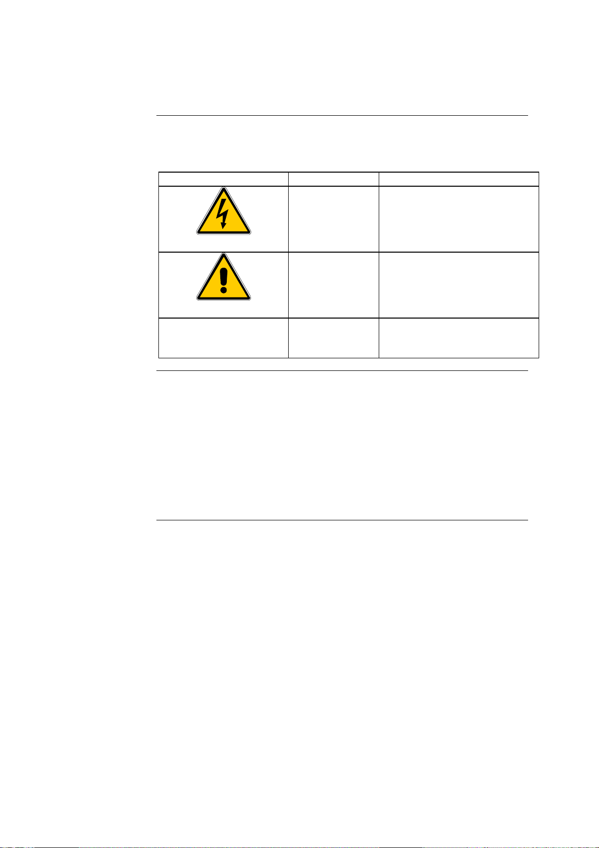
The following symbols and headings are used in this manual:

Symbol Heading Description

WARNING This heading and symbol are

used to indicate that noncompliance with instructions or procedures may lead to injury or even death.

CAUTION This heading and symbol are

used to indicate that noncompliance with instructions or procedures may cause damage to the instrument.

NOTE This heading is used to bring

your attention to topics of importance

• The LightCycler technology is licensed from Idaho Technology Inc., Idaho Falls, ID, USA

• LightCycler is a trademark of Idaho Technology Inc., Idaho Falls, ID, USA, in the United States and some other countries.

• SYBR Green I is a trademark of Molecular Probes Inc., Eugene, OR, USA.

• TaqStart is a trademark of Clontech Laboratories, Inc., Palo Alto, CA, USA

• Expand is a trademark of a Member of the Roche Group.

For License statements, please refer to LightCycler reagent package inserts.

LightCycler Software and License Agreement

Software License Agreement

Program License Agreement

Grant of License

READ THIS LICENSE AGREEMENT BEFORE REMOVING THE PROGRAM CD (HEREINAFTER REFERRED TO AS PROGRAM MEDIA) OR DOCUMENTATION FROM ITS PROTECTIVE COVER. REMOVING THE PROGRAM MEDIA OR DOCUMENTATION WILL CONSTITUTE AGREEMENT TO THE TERMS AND CONDITIONS OF THIS SINGLEUSE, END-USER LICENSE AGREEMENT. IF YOU ARE NOT WILLING TO BE BOUND BY THE TERMS AND CONDITIONS OF THIS LICENSE AGREEMENT, PROMPTLY RETURN THE UNOPENED PACKAGE TO ROCHE DIAGNOSTICS GMBH WITH A COPY OF THE RECEIPT, AND YOUR LICENSE FEE WILL BE REFUNDED.

You assume all responsibility and liability for the selection of this software program, hereinafter referred to as Product, to achieve your intended results, and for its installation and subsequent use.

Roche Diagnostics GmbH hereby grants to Licensee a non-exclusive, singleuse license to use the Product upon the terms and conditions contained in this agreement. You may:

1. Use the Product on a single workstation owned, leased or otherwise con-

trolled by you, whether in a network or other configuration.

2. Make one (1) copy of the Product for backup purposes in support of your

use of the Product on the single workstation.

3. Transfer the Product and license to another party if the other party agrees to accept the terms and conditions of this Agreement. If you transfer the Product, you must, at the same time, either transfer thel copy of Product to the same party, or destroy any copies not transferred.

You must reproduce and include the copyright notice on all copies of the product documentation.

Continued on next page

LightCycler Software and License Agreement,

Grant of Licence (continued)

YOU MAY NOT:

1. use or copy the Product, in whole or in part, except as expressly provided in this Agreement,

2. use the Product on more than one workstation concurrently,

3. copy, rent, distribute, sell, license or sublicense, or otherwise transfer the Product or this license, in whole or in part, to another party, except as specifically set forth in this Agreement,

4. use the Product, or any portion of the Product, to develop, or incorporate into, other software that can be executed without a licensed copy of the Roche Diagnostics Image.

The use of the Product, or any portions of the Product, to develop, or incorporate into, other software capable to executing without a licensed copy of Roche Diagnostics Image, is specifically prohibited under the terms of this Agreement. Further, the use of the Product, or any portion of the Product on more than one workstation at one time is specifically prohibited under the terms of this Agreement. For further information, please contact

Terms

Roche Diagnostics GmbH Roche Molecular Biochemicals Sandhoferstraße 116 D-68298 Mannheim. Germany

The license is effective until terminated. You may terminate this Agreement at any time by destroying the Product together with the copy and documentation in any form. It will also terminate automatically and without notice from Roche Diagnostics GmbH if you fail to comply with any term or condition of this Agreement. You agree to destroy the Product and the copy ,if any, of the Product upon termination of this Agreement.

Continued on next page

LightCycler Software and License Agreement,

Limited Warranty

Limitations of Remedies

The Product is provided as is without warranty of any kind, either expressed or implied, including, but not limited to the implied warranties of merchantability and fitness for a particular purpose. The entire risk as to the quality and performance of the Product is with you as Licensee, should the Product prove to be defective. You assume the entire costs of all necessary servicing, repair, or correction. However, Roche Diagnostics GmbH warrants that the program media on which the software is furnished is free from defects in materials and workmanship under normal use for a period of ninety (90) days from the date of delivery as evidenced by a copy of your receipt. ROCHE DIAGNOSTICS

GMBH MAKES NO FURTHER WARRANTIES OR GUARANTEES NOR EXPLICIT NOR IMPLIED.

Roche Diagnostics GmbH’s sole liability and your sole remedy shall be:

1. the replacement of the program media not meeting Roche Diagnostics GmbH’ s limited warranty and which is returned to Roche Diagnostics GmbH with a copy of your receipt;

2. if Roche Diagnostics GmbH is unable to deliver replacement program media which is free of defects in workmanship, you may terminate this Agreement by returning the Product and a copy of your receipt to Roche Diagnostics GmbH, and your money will be refunded.

In no event will Roche Diagnostics GmbH be liable to you for any damages, including any lost profits, lost savings, or other indirect, special, exemplary, incidental or consequential damages, claims or actions, arising out of the use or inability to use the Product, even if Roche Diagnostics GmbH has been advised of the possibility of such damages, claims or actions. Further, in no event will Roche Diagnostics GmbH be liable for any claim by any other party arising out of your use of the Product.

Continued on next page

LightCycler Software and License Agreement,

General Information

You may not sublicence, assign or transfer the license or the Product, in whole or in part, except as expressly provided in this Agreement. Any attempt otherwise to sublicense, assign or transfer any of the rights, duties or obligations hereunder is void.

• This Agreement will be governed by the laws of Germany.

• Should any part of this agreement be declared void or unenforceable by a

court of competent jurisdiction, the remaining terms shall remain in full force and effect.

• Failure of Roche Diagnostics GmbH to enforce any of its rights in this

Agreement shall not be considered a waiver of its rights, including but not limited to its rights to respond to subsequent breaches.

By opening and using this software you acknowledge that you have read this Agreement, understand it, and agree to be bound by its terms and conditions. You further agree that this agreement is the complete and exclusive statement of the Agreement between you and Roche Diagnostics GmbH and supersedes any proposal or prior agreement, oral or written, any other communications between you and Roche Diagnostics GmbH relating to the subject matter of this Agreement.

Chapter A

Technical Aspects of the LightCycler

Instrument

A 1

1. Technical Aspects of the LightCycler Instrument

1.1 Table of Contents

1.1

1.2

1.3

1.3.1

1.3.2

1.3.3

1.3.4

1.4

2.1

2.2

3.1

3.2

3.3

3.4

3.5

4. Operation and Maintenance of the LightCycler

Technical Aspects of the LightCycler Instrument

Table of Contents LightCycler System Technical Data Specifications of the LightCycler Specifications for Applications Specifications for the Detectors Temperature Control Safety Precautions for the LightCycler

System Description

The LightCycler PC Configuration

Installation

Installation Requirements Installation of the LightCycler Installation of the Computer Installation of LightCycler Software Version 3 Dismantling the LightCycler System

Topic See Page

A 1 A 2 A 3 A 6 A 6 A 7 A 8

A 9 A 11 A 12 A 12 A 16 A 17 A 17 A 19 A 20 A 21 A 29 A 30

A 2

1.2 LightCycler System

Note

Components of the LightCycler System

Using the system improperly may compromise the integrity of the results, result in poor performance, or even permanently damage the equipment.

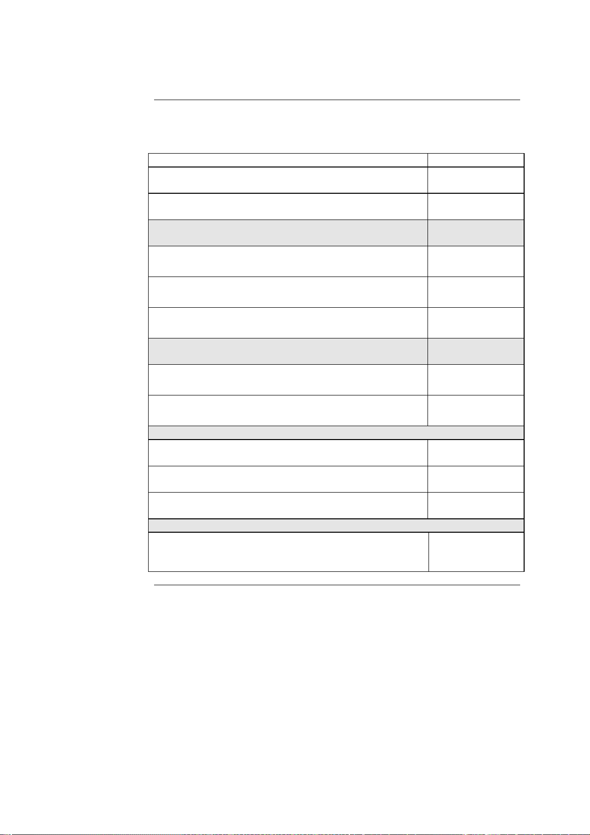
The components of the LightCycler System are listed in the following table. Please note that these components may vary from country to country.

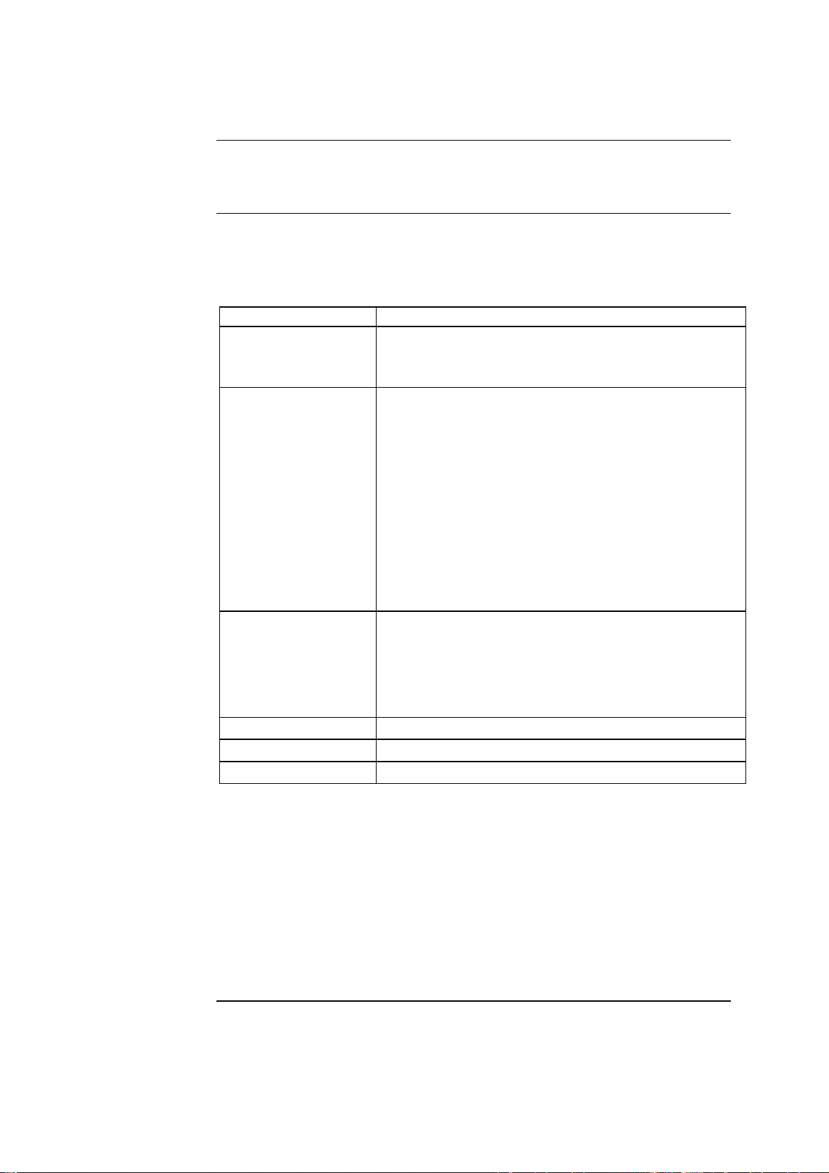
Component Description

System component 1

• LightCycler Instrument

• Sample Carousel (for Ø 1.5 mm capillary)1 pre-

mounted in LightCycler Instrument

System component 2

• LightCycler Capillaries (96 capillaries and stop- pers/box)

• 32 LightCycler Centrifuge Adapters in an alumi- num cooling block

• 1 LightCycler Operator’s Manual

• 1 LightCycler Software Package

• Cable to connect LightCycler Instrument to the computer

• Power Cord (German)

• Power Cord (U.S.)

• Mouse Pad

Hardware

• PC with Pentium processor

• 64 MB SDRAM (minimum configuration)

• 24x CD-ROM drive

• Keyboard and PS/2 mouse

• Internal Iomega ZIP drive

Operating system Monitor Printer

• Windows NT 4.0, including Service Pack III

• 17" monitor

• Hewlett-Packard Color Inkjet Printer

Also available as single components: LightCycler Sample Carousel LightCycler Capillaries LightCycler Centrifuge Adapters LightCycler Software Package

Computer workstation configuration may vary from country to country and

Cat. no. 1 909 282 (1 piece) Cat. no. 1 909 339 (1 set, 768 capillaries) Cat. no. 1 909 312 (1 Set) Cat. no. 1 909 304

may change due to component availability and technical advances. To confirm exact computer configuration, please contact your local Roche Molecular Biochemicals representative.

Continued on next page

A 3

1.2 LightCycler System, Continued

Marks of Conformity

The LightCycler has been manufactured according to EN 61010-1 (Safety regulations for Measuring, Control and Laboratory Instruments; Part 1: General Requirements [IEC 1010-1 + A1: 1992, modified]) and has been checked in accordance with all relevant safety standards prior to leaving the factory.

The instrument has been approved for use by recognized testing institutions. This is confirmed by the following test/conformity symbols:

Acronym Test Symbol Testing Institution

Certified by TÜV Product Service

The instrument conforms to current directives as issued by the European Union

Certified by Underwriters Laboratories Inc.

CUL

Equipment to be connected must fulfill the standards set by IEC 950 (Information security in technical equipment, including electronic business machines).

Certified by Underwriters Laboratories for Canada – a testing facility recognized by the Standards Council of Canada (SSC)

Continued on next page

A 4

1.2 LightCycler System, Continued

Classification

Note on Use with Infectious Material

The LightCycler Instrument is classified as:

• ISM instrument (Industrial Scientific Medical Device), medium-sized, for industrial, laboratory and domestic use.

• Designed for stationary operation.

• Intended for worldwide use.

• Intended for evaluating preprocessed biological material.

• The instrument may not be used to analyze infectious materials unless ad-

ditional safety measures to ensure safe sample handling (e.g., placing the instrument in a laminar flow biological safety cabinet) are taken beforehand.

A 5

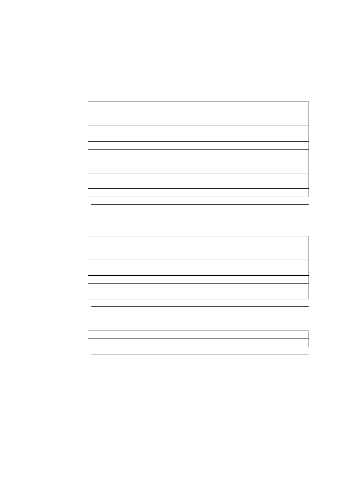
1.3 Technical Data

1.3.1 Specifications of the LightCycler

General Data

Environmental Parameters

Dimensions Length:

Width:

Height: Weight 19.2 kg Power supply 110–240 V, +/–10%, 47–63 Hz Wattage max. 800 W Maximum current Europe:

US: Noise in accordance with DIN 43635 <60 dBA Heat emission, including PC, monitor and printer Safety symbols CE, GS, UL, CSA or CUL

Temperatures allowed during operation 15° to 35°C Temperatures required to maintain specifications during operation Temperatures allowed during transportation/storage/packaging Relative humidity 20 to 80%, no condensation Altitude/pressure 0 to 2000 m above sea level,

max. 850 W

18° to 30°C

–20° to +60°C

1030 to 850 hp

45 cm 30 cm 40 cm

4 A (220 V) 8 A (110 V)

Samples

Number of samples per run 32 Sample volume 10 to 20 µl

A 6

1.3.2 Specifications for Applications

Temperature for PCR

Temperature range 40° to 98°C Accuracy of “capillary temperature” at thermal equilibrium Accuracy of “displayed temperature” with respect to capillary temperature at thermal equilibrium

Capillary Heating Rates Volume : Heating

Heating rate 40° to 95°C (non-linear)

Heating rate 50° to 72°C (non-linear)

Heating rate 72° to 95°C (non-linear)

Capillary Cooling Times Volume : Cooling

Cooling rate 95° to 40°C (non-linear)

Cooling rate 95° to 60°C (non-linear)

Temperature Tolerances, Short Term

Precision of capillary temperature over all capillary positions when measured for 30 s at 95°C Precision of capillary temperature over all capillary positions when measured for 30 s at 70°C Precision of capillary temperature over all capillary positions when measured for 30 s at 45°C

Temperature Difference, Melting Curves

Systematic difference between sensor temperature and capillary temperatures when chamber is heated from 50°C to 95°C at a rate of 0.2°C/s

±0.4°C ±0.4°C

Time Required

10 µl: ≤13 s 20 µl: ≤15 s

10 µl: ≤6 s 20 µl: ≤8 s 10 µl: ≤6 s 20 µl: ≤8 s

Time Required

10 µl: ≤23 s 20 µl: ≤24 s

10 µl: ≤7 s 20 µl: ≤7 s

±1.5°C ±1.0°C ±0.5°C

<0.1°C

A 7

1.3.3 Specifications for the Detectors

Excitation

Type LED Median wavelength 470 nm Wattage at 470 to 490 nm 0.1 mW

Filter

Detector 1 Bandpass 530 nm, HBW 20 nm, dichroic Detector 2 Bandpass 640 nm, HBW 20 nm, dichroic Detector 3 Bandpass 710 nm, HBW 40 nm, dichroic

Detector

Type Photohybrid Sensitivity at 530 nm, 20 µl sample volume 10 fM fluorescein Resolution 12 bit Range of detection sensitivity Adjustable by a factor of 1 to

256

Typical Time

Signal acquisition time for 32 capillaries

≈ 5.0 s

A 8

1.3.4 Temperature Control

Visual Display of Temperature Profiles

The LightCycler software graphically displays the current temperature in the thermal chamber. These graphs appear under Temperature History on the Running Screen (see below). The graphs show “overshoots” and “undershoots” for each temperature transition (see arrows below).

A 9

Continued on next page

1.3.4 Temperature Control, Continued

100

Temperature [ C]

200

Fluid temperature in capillary

Ambient temperature in thermal chamber

Autocorrection

Effectiveness of Autocorrection

Autocorrection compensates for physical differences in heat capacity in air and water. This specific autocorrection ensures that every programmed temperature is adjusted within the sample capillaries during thermal cycling.

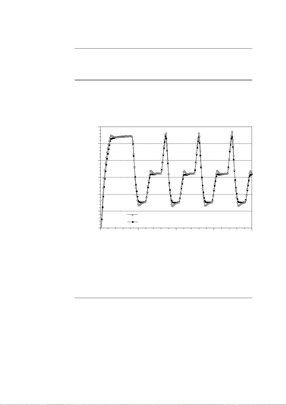
The graph below shows the changes in temperature in both the thermal chamber and a sample capillary during thermal cycling. Differences at any given time between the temperature in the two locations are shown as spaces between the two temperature curves.

0 50 100 150

Time [sec]

Conclusion: This graph demonstrates that:

• The temperature profile shown under Temperature History on the Running Screen exactly corresponds to the capillary temperature, and

• The fluid temperature in the capillaries coincides with the programmed profile.

A 10

1.4 Safety Precautions for the LightCycler

General Safety Precautions

Always observe these precautions when using the LightCycler Instrument:

• Follow all safety instructions printed on, or attached to, the analytical in- struments.

• Observe all general safety precautions which apply to electrical instruments.

• Never touch switches or power cord with wet hands.

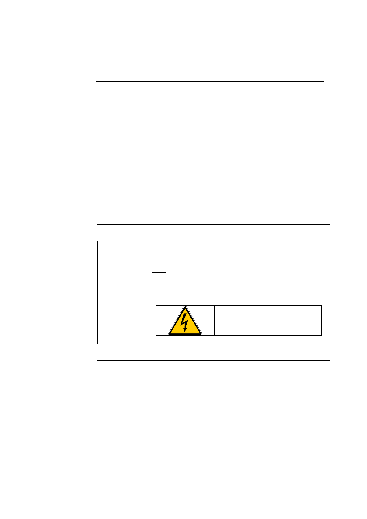
• Do not open the housing of the LightCycler.

Note: Only authorized service personnel should perform service or repairs required for this unit.

• Do not open the LightCycler thermal chamber during operation.

• The chamber lid and the sample rotor are hot while the instrument is op-

erating. Note: The corresponding symbol is attached to the front side of the LightCycler.

• Always wear safety goggles and gloves when dealing with toxic, caustic, or infectious materials .

• When analyzing infectious materials, use the LightCycler only in specially equipped rooms with controlled exhaust equipment, e.g., biological safety cabinets.

Safety Precautions for Centrifuge Adapters

Loading capillaries to perform fluorescence measurement with the LightCycler requires a centrifugation step in a tabletop centrifuge with specially designed adapters. A centrifuge adapter with capillary weighs approximately 6.2 grams. Always observe the following precautions during the centrifugation step:

• Always distribute the adapters in the rotor so the weight in the rotor is balanced, and

• Adjust the speed of the centrifuge so the centrifugal force does not exceed 700 x g.

Note: For details on the maximum weight that can be processed in your centrifuge, refer to the product specification sheet for that centrifuge.

A 11

2.1. The LightCycler

Schematic of the LightCycler

2. System Description

A 12

Continued on next page

2.1 The LightCycler, Continued

Description of the Instrument

Communication between LightCycler and PC

The LightCycler basically consists of an upper unit and a lower unit. The upper unit contains the heating coil. The lower unit contains the thermal chamber, fluorimeter, drive units, electronic boards and power supply. The various elements are mounted on a 10-mm cast aluminum base plate. This guarantees stability, especially for the thermal chamber and fluorimeter. Hot or ambient temperature air, introduced into the thermal chamber, regulates the temperature of the sample capillaries. A heating coil heats the air, which is then fed into the chamber by a fan. The fan ensures efficient air circulation and temperature homogeneity during the heating cycle. During the cooling cycle, the fan operates at a higher speed to ensure adequate cooling. During measurements, a stepper motor rotates the sample carousel to position the capillary tip precisely at the focal point of the fluorimeter optics. The fluorimeter itself is positioned radially to the maximum signal to compensate for any radial deviation of the capillary tip.

For online display, data are transmitted to and from the PC via a serial interface. Control is made possible by three microprocessors that are integrated into the instrument:

• Processor 1 is for communication,

• Processor 2 regulates the temperature, and

• Processor 3 controls the measurement procedures as well as the move-

ment of the rotor and fluorimeter.

Users enter data on samples (number of samples, name, concentration, etc.) and on the experimental protocol into the PC; the PC transmits the data to the LightCycler. The PC also monitors the temperatures and fluorescence signals during the PCR run and operates all the analytical programs.

Power Supply Unit

All high-voltage components are located in the power-supply unit. Note: Electrical safety information and test symbols apply to this unit. To minimize interference to the detector electronics, the electronics that control the drive units are located on a separate circuit board.

Continued on next page

A 13

2.1 The LightCycler, Continued

Temperature Setting of the Thermal Chamber

Fluorimeter

Temperature is controlled with hot air and air at ambient temperature. Varying the voltage supplied to the heating coil regulates the temperature. A sensor provides reference values for control purposes. During the heating phase, the fan in the thermal chamber operates at low speeds to ensure homogenous distribution of temperature. During the cooling phase, the fan operates at higher speeds so that the capillaries and the heating coil can be cooled efficiently. Two sensors are integrated into the LightCycler to prevent unduly high temperatures:

• Sensor I is located in the thermal chamber and switches off the heat when a

temperature of 125°C has been reached.

• Sensor II monitors the temperature on the aluminum base plate, and

switches off the entire LightCycler to protect the electronics when the temperature exceeds 55°C.

A three-channel fluorimeter is used for detection purposes. A blue diode (LED) with maximum emission of 470 nm serves as the energy source for sample excitation. Screens are used to diffuse the light emitted by the LED to ensure uniformity. The exhaust and ventilation channels have been designed to prevent ambient light from entering directly into the thermal chamber. Fluorescence is detected at 530 nm, 640 nm, and 710 nm with the aid of photohybrids. Note: Acquisition time for fluorescence acquisition time is 20 msec (16.6 msec in the U.S.).

Measurement of Samples

The thermal chamber and the fluorimeter are placed optimally for sample measurement. Only the sample carousel, which holds the capillary, rotates during measurement of the various samples.

Continued on next page

A 14

2.1 The LightCycler, Continued

LightCycler Diodes

Position of

Diode

Top Power on Green On Instrument is switched on

Middle Cycling Red On Instrument is running

Bottom Run Yellow On PCR run is completed

Three diodes are located at the front of the LightCycler. All of the diodes come on when the instrument is switched on. In this way, the instrument tests for proper functioning of the diodes. During instrument operation, the diodes function as described in the table below:

Label Color of Diode Function Indication

Off

Flashing Instrument is defective

completed Off Instrument is running

• No power

• Instrument is defective

A 15

2.2 PC Configuration

General

The computer workstation contains the following components:

Hardware

• PC with a Pentium processor

• 64 MB SDRAM (minimum configuration)

• 24x CD-ROM drive

• Keyboard and PS/2 mouse

• Internal Iomega ZIP drive

Operating system Monitor Printer

Computer workstation configuration may vary from country to country and

• Windows NT 4.0, including Service Pack III

• 17" monitor

• Hewlett-Packard Color Inkjet Printer

may change due to component availability and technical advances. To confirm exact computer configuration, please contact your local Roche Molecular Biochemicals representative.

A 16

3. Installation

3.1 Installation Requirements

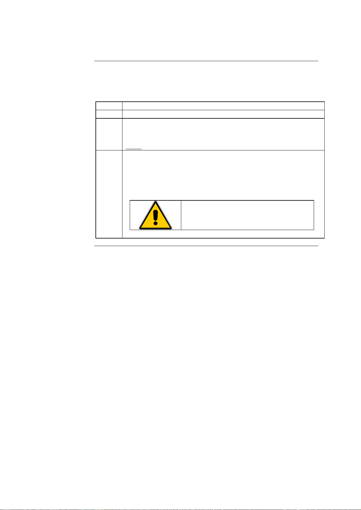
Note

Space and Power Requirements

• Do not place the LightCycler next to instruments that cause electromag- netic interference or have high inductance (e.g., centrifuges or mixers).

• Peripheral instruments connected to the LightCycler System must meet the IEC 950 (UL 1950) standard.

• All plugs used in the LightCycler System (PC, printer, monitor) should have the same phasing in order to prevent switch-on peaks and electronic noise generated by other instruments or by the power supply itself. We recommend using a dedicated multiple-outlet surge protector for the LightCycler System.

• Use only the supplied power lines and RS 232 connector.

Place the instrument in a site that can support the following instrument requirements:

Dimensions The LightCycler is 30 cm wide, 45 cm long, and 40 cm

high. . Weight Approximately 20 kg Voltage Requirements

The LightCycler operates between 120 and 240 V (50 to 60

Hz).

Note: The LightCycler adjusts automatically to the avail-

able voltage when the instrument is plugged in. The user

does not have to set the instrument to the correct voltage

manually.

Power Consumption

Do not open the LightCycler housing.

The LightCycler uses 800 W max.

PC and printer consume an additional 500 W (approx.).

Continued on next page

A 17

3.1 Installation Requirements, Continued

Environmental Parameters

Storage Conditions

The instrument requires the following environment for accurate operation:

Ambient temperature 15° to 35°C Ambient temperature required to main specifications during operation Humidity 20 to 80%, no condensation Altitude Sea level to 2000 m Excess voltage Category II Degree of contamination 2

The LightCycler can be stored under the following conditions:

Ambient temperature –20° to +60°C Humidity 20 to 80%, no condensation

18° to 30°C

A 18

3.2 Installation of the LightCycler

Installation of the LightCycler Instrument

Your Roche Molecular Biochemicals representative will normally install the LightCycler Instrument at your site. Should this not be possible, follow these steps to install the instrument successfully:

Step Action

1 Unpack the instrument. 2 Position the instrument on the workbench. Allow 10-cm spaces to

the left, right and behind the instrument to ensure sufficient cooling of the electronic components. Note: The workbench should not be covered with paper.

3 Make the following electrical connections:

• Connect the LightCycler to the PC using the RS 232 cable (serial interface) provided with the system.

• Connect the LightCycler, PC, monitor, and printer to the same multiple-outlet distributor plug.

Ensure that PC, monitor, and printer have been set to the correct voltage.

A 19

3.3 Installation of the Computer

Installation of the PC

To install the PC, do the following:

Step Action

1 Connect mouse, keyboard, and monitor to the computer. 2 Connect the LightCycler to the computer with the RS 232 cable

(serial interface) provided with the system.

3 Connect the computer, monitor, and LightCycler to the same

multiple-outlet distributor plug. The computer is now ready for operation.

A 20

3.4 Installation of LightCycler Software Version 3

Logging In

Installation of LightCycler Software

A prerequisite for the software installation is that the operating system WINNT 4.0 (Service Pack 3) has been installed. For the installation of the software and the setting up of users it is recommended that you log in as administrator. All instructions are based on the English WIN NT 4.0 version. The operating system programs and folders in the German versions have different names.

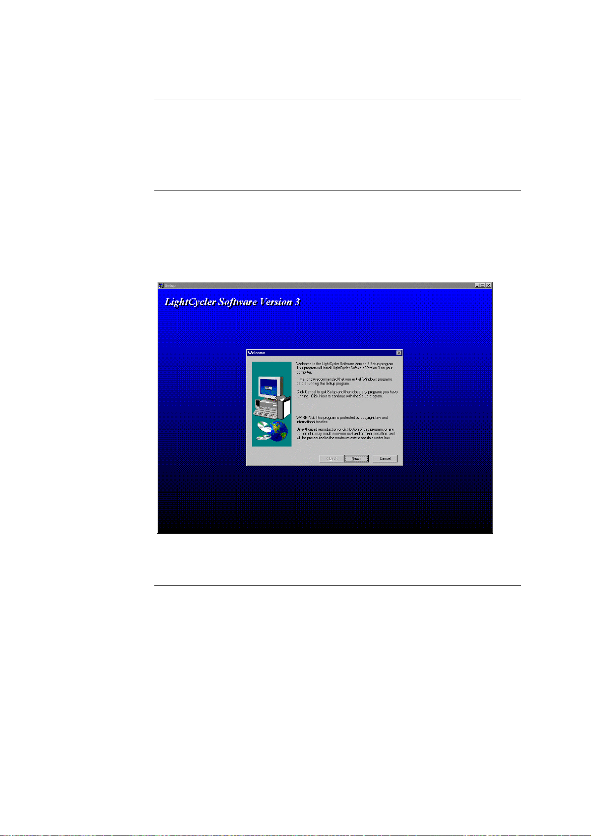
Insert the CD with the LightCycler Software version 3 into the CD-ROM drive of your computer. The autorun function will automatically start the Setup program. If the autorun function is not available, the CD must be opened from the Explorer, and the 'setup' program started manually by doubleclicking on it. The Setup program displays the following start screen:

Click the “Next” button to continue with the installation. Click “Cancel” to abort the program.

Continued on next page

A 21

3.4 Installation of LightCycler Software Version 3, Continued

License Agreement Information of LightCycler Software

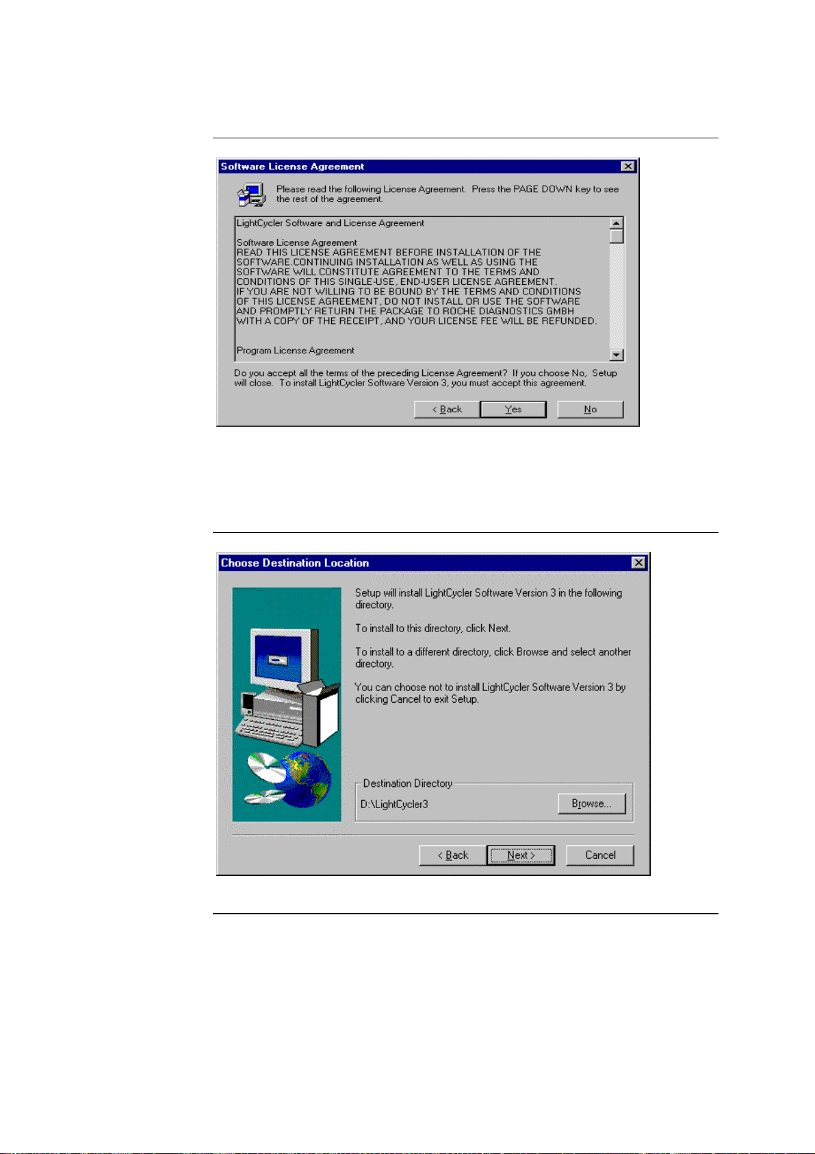
Here, the customer is provided with a display of the license agreement. Scroll bars can be used to view the entire text. Choose “Yes” to accept the license agreement. If you choose “No”, the program will be exited. Clicking on “Back” will redisplay the start screen.

Installation Directory of LightCycler Software

Continued on next page

A 22

3.4 Installation of LightCycler Software Version 3, Continued

Installation Directory of LightCycler Software,

Continued

The software will be installed to the recommended directory “LightCycler3”. The disk drive corresponds to the drive to which WIN NT was installed, here: drive “D”.

If “Next” is clicked on, the installation will be continued. If “Cancel” is chosen, the installation will be exited, and “Back” will redisplay the previous screen.

If you wish to change the disk drive or the directory, click the “Browse” button. A popup window will display permitting the desired path and directory to be entered.

The installation to the “LightCycler3” directory will have no consequence for any previous installations of version V1.22 since that version was installed in the directory named “LightCycler”. It is therefore recommended that directory “LightCycler3” be used so as to avoid any conflict with respect to future versions and to be able to quickly locate the relevant versions.

Continued on next page

A 23

3.4 Installation of LightCycler Software Version 3, Continued

LightCycler Software Program Folder

The program folder contains icons to start the various LightCycler Programs. A folder named “LightCycler3” is set up in the Start menu under 'Programs'. This name should be retained, if possible, to be able to locate the folder quickly.

Click “Next” to continue with the installation. If “Cancel” is chosen, the installation will be exited, and ”Back” will redisplay the previous screen.

Starting the LightCycler Software Installation

Prior to the start of the installation, a summary of the current settings is displayed. You are provided with one last chance to make changes, or to exit the installation. Click “Next” to start the installation. If “Cancel” is chosen, the installation will be exited, and 'Back' will redisplay the screen below.

Continued on next page

A 24

3.4 Installation of LightCycler Software Version 3, Continued

Starting the LightCycler Software Installation, Con-

tinued

LightCycler Software Installation Progress

After the start of the installation, a progress bar is displayed indicating the progress of the installation. Please wait until the installation is complete and the “Setup Complete” screen appears.

It is possible to exit the installation by clicking “Cancel”. This should, however, only be done in emergencies. Any program parts that have been installed up to this point will not be removed automatically.

At the end of the installation, the program registration takes place. A start icon for the “Front” program will be installed on the desktop and added to the Start menu. The folder “LightCycler3” containing the programs

“Front”, “BMRun” and “LCDA” will be set up in the Start menu under “Programs”.

Continued on next page

A 25

3.4 Installation of LightCycler Software Version 3, Continued

LightCycler Software Installation Progress, Continued

Terminating Setup

The installation has been carried out successfully. Click “Finish” to complete the Setup program. If the check box “Launch the program file” is selected, the

LightCycler program “LightCycler3 Front Screen” (Front) will start when the “Finish” button is clicked.

A 26

Continued on next page

3.4 Installation of LightCycler Software Version 3, Continued

System File For the LightCycler3 program to be able to run, the system file “mfc42.dll” is

required. If an earlier version of this file is installed on your computer, it will be overwritten with the more recent version in the directory

Winnt\system32\.

Acrobat Reader

Num2Dot

The Acrobat Reader is required to be able to read the Help files. This program is also included on the CD. It needs only to be installed if the program has not previously been installed on the computer.

To install Acrobat-Reader, open the CD from the Explorer and start the “ar40eng” program by double-clicking on it in the “Acrobat Reader” subdirectory. The installation procedure is similar to that of the LightCycler Software.

Num2Dot is a tool that allows use of the “comma” of the numerical pad of your keyboard to enter a decimal point. As the LightCycler Software is designed to be run under english country settings, the Software expects a “point” as a decimal point. The ability to convert the decimal “comma” on a variety of non-english keyboards to write a “point” instead significantly improves the convenience of the system. Note: It is not required to install Num2Dot if your keyboard´s numerical pad is equipped with a “point” as decimal point.

To install Num2Dot, open the CD from the Explorer and start the install Num2Dot by double-clicking “Setup.exe” in the “Num2Dot” subdirectory. The installation procedure is similar to that of the LightCycler Software.

Num2Dot will automatically be started whenever you launch Windows-NT on your PC. Verify activation of the numerical pad on your keyboard. The green light built into the “Num” key must be on. After installation of Num2Dot, the “comma” key will be converted to a “point” key. The Short cut command “AltGr + DecimalComma” can be used to deactivate Num2Dot, as well as to reactivate the conversion.

Continued on next page

A 27

3.4 Installation of LightCycler Software Version 3, Continued

Uninstall To uninstall programs under WIN NT, use the “Add/Remove Programs”

tool. This auxiliary program appears in the Start menu under Settings-Control Panel. A list of the programs installed is displayed. Select the program you wish to uninstall from the list and remove it by clicking the “Add/Remove” button.

A 28

3.5 Dismantling the LightCycler System

Dismantling the System

To dismantle the LightCycler system, do the following:

Step Action

1 Switch off the instrument. 2

3 Ship instrument in its original packaging.

• Disconnect the RS 232 cable and power cables.

• Clean the instrument (according to the guidelines in Topic 4 of

this chapter).

• Decontaminate the instrument if necessary.

A 29

4. Operation and Maintenance of the LightCycler

Guidelines for Operation

Transport and Storage

• The LightCycler instrument should only be operated in locations which are protected from the weather. It may not be operated in buildings that lack facilities for regulating temperature. If necessary, additional drying agents may be used to eliminate humidity. Neither ice nor moisture should be allowed to form on the instrument.

• The instrument should be placed on an even work surface and protected from direct sunlight and outside light.

• The instrument should not be operated near dripping, spraying, splashing or running water.

• The instrument is suitable for use according to classification 3K3 in accor- dance with Standard EN 60721-3-3.

• The instrument should be protected from effects generated by fauna and flora.

• The instrument may be used at locations subject to noticeable or signifi- cant vibration. However, it should not be exposed to higher levels of shock waves.

• The instrument is suitable for use according to classification 3M4 in ac- cordance with EN 60721-3-3. The instrument is able to tolerate vibrations up to classification 3M6.

When storing or transporting the instrument, do not allow it to be exposed to extreme cold (e.g., placing it in an airfreight cargo bin). Avoid temperatures lower than –25°C (since such temperatures may damage optical systems). The optical systems have open ventilation systems and should therefore be protected from dirt and humidity.

Guarantee

The terms of the guarantee are incorporated in the purchase agreement. For further details, please contact your Roche Molecular Biochemicals representative.

Continued on next page

A 30

4. Operation and Maintenance of the LightCycler, Continued

General Maintenance

Cleaning the Instrument

The instrument is maintenance-free.

• Use 70% ethanol for disinfecting the thermal chamber.

• Clean the optical window with alcohol and an optical polishing cloth.

• Clean the housing with a mild commercial household detergent.

• Use a mild commercial household detergent for cleaning the housing.

• Do not pour fluids into the thermal chamber.

A 31

B 1

Chapter B

LightCycler Software

Version 3

B 2

1.1. Table of Contents

1. Software

Topic See Page

1. Software

1.1 Table of Contents B 2

1.2 Introduction B 4

1.3 The Front Screen B 7

1.4 Functions of Buttons on the Front Screen B 8

1.5 Edit Graphics Defaults Window B 9

2. Programming a Run

2.1 Programming Screen B 11

2.1.1 Menu Options Available on the Programming Screen B 14

2.1.2 Programming Screen: User / Experiment Window B 17

2.1.3 Programming Screen: Experiment / RUN / EXIT Window B 19

2.1.4 Programming Screen: Sample Data Entry B 21

2.1.4.1 Loading Screen Activated by the Edit Samples Button B 22

2.1.4.2 Naming Samples at the Beginning of a Run B 25

2.1.5 Real Time Fluorimeter (RTF) B 29

2.1.6 Programming Screen: Color Compensation Window B 32

2.1.7

Programming Screen: Display Mode / Fluorimeter Gains Window

B 1

B 11

B 34

2.1.8 Programming Screen: Cycle Program Data and Temperature Targets Window

2.1.9 Programming Screen: Graphic Simulation Window B 40

2.1.10 Programming Screen: Cycle Program Overview Window B 41

3. Running the LightCycler

3.1 LightCycler Run Screen B 42

Continued on next page

B 36

B 42

B 3

1.1 Table of Contents (continued)

Topic See Page

4. Data Analysis

4.1 Introduction B 46

4.2 Select Data File / Data Analysis Window B 47

4.3 LCDA Front Screen B 49

4.3.1 LCDA Front Screen: Temperature vs. Time Graph B 50

4.3.2

4.3.3 LCDA Front Screen: Using Color Compensation Files B 54

4.4 LCDA Front Screen: Data Retrieval B 56

4.5 Further Analysis B 56

Fluorescence vs. Cycle Number / Time / Temperature Graph

B 46

B 52

5. Display and Analysis of Quantification Data

5.1 Introduction B 57

5.2 Quantification: Selection of Analysis Method B 58

5.3 Quantification Step 1: Baseline B 61

5.4 Quantification Step 2: Noise Band B 64

5.5 Quantification Step 3: Analysis B 66

5.6 A Procedure for Analyzing Quantification Data B 72

6. Display and Analysis of Melting Curve Data

6.1 Introduction B 85

6.2 Melting Curve Step 1: Melting Peaks B 87

6.3 Melting Curve Step 2: Peak Areas B 91

6.4 Melting Curve Step 3: Manual T

6.5 A Procedure for Analyzing Melting Curve Data B 95

B 57

B 85

B 93

B 4

1.2. Introduction

Before Beginning

Program Start

Your LightCycler should have been installed and set up according to the instructions described in Section 3 of Chapter A. During installation, the LightCycler software will automatically be loaded into the part of the hard disc that contains the Windows NT operating system.

Prior to the start of the program, an account must be set up for each user

granting him access privileges that enable him to use the computer. Such accounts must be used by the users to log on to Win NT.

If the check box 'Yes, launch the program file' was selected at the end of the

installation, the 'LightCycler3 Front Screen' (Front) program will now start.

Log On Procedure

The current user may log on using the 'Log On As Different User' button.

The information message to the effect that all programs will be closed must be acknowledged by clicking 'OK'. Subsequently, all programs are closed and WIN NT displays its log-on screen. The user must now log on by entering his user name and password. Note: The LightCycler does not allow to log on as a different user as long as a LightCycler Run is performed to prevent loss of data by interrupting the run.

Continued on next page

B 5

1.2. Introduction, Continued

Program Start, In the event that the check box 'Yes, launch.....' was not selected at the end

of the installation, the user needs to log on first. This may be accomplished in the Start menu using the 'Shut Down' command.

Select the option button 'Close all Programs and log on as different user'

and click the 'Yes' button. Windows now closes all programs and displays its log-on screen. The user must now log on by entering his user name and password.

Following the log-in procedure, the LightCycler3 program may be started.

The start should always be carried out from the desktop or the Start menu by clicking the 'LightCycler3 Front Screen' icon. Only this procedure will ensure that the user is logged on properly to the program and that the required work directories are created upon the initial startup.

Continued on next page

B 6

1.2. Introduction, Continued

How to Start Follow the steps in the table to start.

Step Action

1 Turn on the computer by pressing the power button on the front

of the computer. Result: Windows NT will automatically load.

2 Type in your User Name and Password to log into Windows NT

and the LightCycler software. Note: User management requirements for the LightCycler software are set up through the Windows NT operating system.

3 4

Flip the switch on the back panel of the LightCycler to the On position. Click on the LightCycler 3 Front Screen icon; this will bring up the

LightCycler Front Screen.

Note: Alternatively, you may use Windows NT Explorer to start each software function independently, without first entering the LightCycler Front Screen. For instance, from Windows NT Explorer, do the following:

Important Note about the PC

To start from... Click on...

LightCycler Front Screen Programming / Run Screen LightCycler Data Analysis Front Screen

Tip: Accessing the screens through Windows NT Explorer allows you to graphically display and evaluate data generated in previous experiments while other experimental protocols are in progress.

The PC supplied with the LightCycler should be used exclusively with the LightCycler software. We strongly advise against installing and running additional software on this PC.

Front.exe

(BM) Run32.exe

LCDA.exe

Continued on next page

B 7

1.3. The Front Screen

LightCycler Front Screen

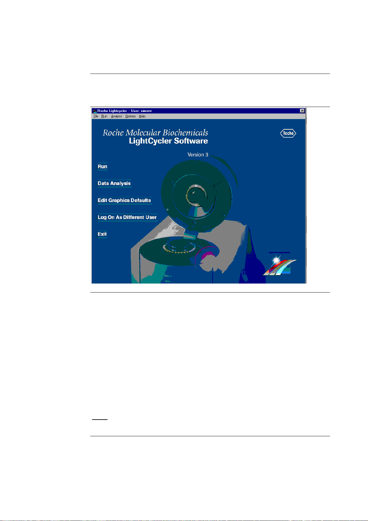
In Version 3 of the LightCycler software, the front screen looks like this:

Introduction When you click on the LightCycler Front Screen icon on the Windows NT

desktop, the LightCycler software is activated and the LightCycler Front Screen will appear on the monitor. This screen provides access to the functions of the LightCycler software via a set of menus.

Alternatively, you may also directly access the most important instrument functions by clicking on these screen buttons:

• Run

• Data Analysis

• Edit Graphics Defaults

• Log On As Different User

• Exit

Note: The functions of these buttons are explained in more detail on the pages of the next section.

B 8

1.4. Functions of Buttons on the Front Screen

Run Button The Run button starts the LightCycler Run Software which allows you to

program and execute cycle experimental protocols. Note: The Front Screen Run menu may be used for the same purpose.

Data Analysis Button

Edit Graphics Defaults Button

Log On As Different User Button

The Data Analysis button provides access to the LightCycler Data Analysis (LCDA) software.

Note: The Front Screen Analysis menu may be used for the same purpose.

The Edit Graphics Defaults button allows a user to change the colors and line styles used in the data display graphs (see Section 1.5 of this chapter).

Note: The Front Screen Options menu may be used for the same purpose.

Each user only has access to a unique set of files. To access files belonging to a different user, click on the Log On As Different User button. This allows you to exit all LightCycler programs and reactivate the software with a different user name and password (as prompted by the system).

Note: The LightCycler does not allow to log on as a different user as long as a LightCycler Run is performed to prevent loss of data by interrupting the run.

The Front Screen Options menu may be used for the same purpose.

Exit Button The Exit button allows you to quit the LightCycler program.

Note:

• You may also quit the program by closing the Front Screen window. The

Exit function is also part of the Front Screen File menu.

• After exiting the software, you still must turn off the LightCycler instrument separately.

Help Menu The Operator Manual can be called by Acrobat Reader.

Note: Acrobat reader 4.0 is provided as part of the Software CD.

B 9

1.5. Edit Graphics Defaults Window

Edit Graphics Defaults Window

The Edit Graphics Defaults button allows a user to change the color and style of the line used to represent each sample in LightCycler data displays. When you click on the button, the Edit Graphics Defaults window will appear (as shown below):

Continued on next page

B 10

1.5. Edit Graphics Defaults Window, Continued

Changing the Line Display

After entering the Edit Graphics Defaults window, change the appearance of the graph lines as follows: Caution: Changes made to graphics defaults will not be accepted if the LightCycler Data Analysis (LCDA) software is active. Before changing the graphics defaults, first close LCDA. Then, edit and save your graphic defaults and reload LCDA. The changes are then accepted by LCDA. User specific default settings are stored in a file „defaults.ini“ in the user directory. You may store your settings with another user by copying your user default.ini file into the other user directory.

Step Action

5 If you do not like the appearance of the sample lines in the data

Right-Click on the sample number you wish to change. Result: A pop-up menu will appear. The menu contains the following graphics options: Color, Point Style and Line Style. From the menu, click on the display option you wish to change. Result: One of the Graphics Default Options windows (pictured below) will appear. Click on the option you prefer and then click the OK button. Result: The Graphics Default Options window will close. Note: Changes made to the graphic defaults of one user do not affect the graphics defaults of any other user. From the Edit Graphics Defaults window, click on the Save button to save your new graphics defaults. Note: After saving them, you may always return to your display options (defined in Steps 1–4) at any time by clicking on the Restore button (in the Edit Graphics Defaults window).

display, you may open the Edit Graphics Defaults window and do one of the following:

• Click on the Restore Defaults button to return all options to the system default settings.

• Repeat Steps 1–4 above and choose different options.

Graphics Default Options Windows: Color, Point Styles and Line Styles

B 11

2. Programming a Run

2.1. Programming Screen

Introduction The descriptions given in the following pages explain how to use the

Programming Screen for:

• Defining the parameters of a PCR protocol,

• Starting a PCR run, or

• Viewing online a PCR experiment that is currently in progress.

Activation of Programming Screen

To set up a new experimental protocol or to order a new run with a protocol that has already been defined and stored, you must first activate the Run function from the LightCycler Front Screen. Follow the steps below to activate the Run function and open the Programming Screen:

Step Action

Click the Run button on the LightCycler Front Screen. Result: A data-entry screen opens. This screen will henceforth be referred to as Programming Screen.

If you have not already switched on the LightCycler instrument, the software will prompt you to do so.

Note: It is possible to ignore this message, by simply clicking OK. This will allow you to become familiar with the LightCycler software without running an experiment.

Continued on next page

B 12

2.1. Programming Screen, Continued

Programming Screen

Functions Available on the Programming Screen

Defining Cycle Programs

The rest of the topics in Section 2.1 of this chapter describe the software functions that may be activated by either using the menu bars or clicking on various buttons available on the Programming Screen. Menu options are listed in the top-to-bottom order in which they appear on each menu. Function buttons are described according to the screen areas in which they appear.

Note: Use the Programming Screen diagram above to locate the screen areas, menus, and buttons as they are described below.

Use the Programming Screen to define the cycle programs for an Experimental Protocol (*.exp-file). Once you have defined your Experimental Protocol, you will be ready to run a LightCycler experiment.

Tip: You can use the descriptions in the following sections to familiarize yourself with the actions necessary to define an Experimental Protocol. For instance, as you read the descriptions below, you may activate each function by clicking on the menu option or button, and then enter typical experimental parameters in the tables or fields that appear.

Continued on next page

B 13

2.1. Programming Screen, Continued

Program 3:

Melt

Program 1:

Program 2:

Amplification

Program 4:

Cooling

Initial

Denaturation

Definitions: Protocol / Program / Segment

Experimental Protocol

An Experimental Protocol in general contains one or more Cycle Programs. In the PCR profile shown above, a typical Experimental Protocol contains four programs: 1) an Initial Denaturation Program, 2) an Amplification Program, 3) a Melting Program and 4) a Cooling Program.

A Program (e.g. Cycle Program) contains several Temperature Segments, each of which defines the time and temperature parameters that will be used for denaturation, annealing, extension and/or melting, cooling as well as the fluorescence acquisition mode used to monitor the amplification signal.

B 14

2.1.1. Menu Options Available on the Programming Screen

Options Available on the Programming Screen Menus

The Menu bar on the Programming Screen offers a variety of options for programming, managing, and displaying Experimental Protocols (*.exp- files). The following list gives you a brief description of the menu functions. Note: You may also activate a number of the options listed on these menus key by clicking the buttons found in various areas on the screen. The use of these buttons is discussed in detail in later sections of this chapter.

Menu Offers these options

File Allows you to:

• Create or Open existing *.exp-files,

• Save the current *.exp-file,

• Print the current window contents, and

• Exit the Run program.

Note: Experimental files (*.lin-files) made with older versions of LightCycler software will be automatically converted to *.exp-files when they are first opened.

If you had used the Lightcycler Software 1.2x, we recommend converting all *.lin-files into *.exp-files and then deleting the *.lin- and *pro-files. As a *.profile may have been used by several *.lin-files, *.profiles should only be deleted after converting all *.linfiles.

Edit

Allows you to:

• Cut, Copy, and Paste,

• Edit Sample Defaults ,

• Display Cycle Program Simulation,

• Edit Experimental Notes to your *.exp-files, and

• Show Experimental Notes.

Note: The Cycle Program Simulation and Experimental Notes will appear in the window in the right portion of the Programming Screen under the User / Experiment window.

Continued on next page

B 15

2.1.1. Menu Options Available on the Programming Screen,

Continued

Options Available on the Programming Screen Menus (continued)

Menu Offers these options

Tools

Options

Allows you to:

• Display the Real Time Fluorimeter, and

• Activate a Service Utility function.

Note:

1) The Real Time Fluorimeter option permits continuous fluorescence measurement of samples to allow adjustment of fluorimeter gain by the user.

2) The Service Utility function facilitates adjusting and testing to permit the instrument to be serviced by an authorized specialist from Roche Molecular Biochemicals Technical Support.

Caution: Do not activate the Service Utility function unless Roche Molecular Biochemicals service personnel ask you to do so. Settings of the Service Utility function will not be stored and used by the Run program.

Allows you to:

• Choose (color compensation,-*.ccc-)-files

containing color compensation data, or

• Disable (color compensation,-*.ccc-)-files,

• Set LED Power (to turn the LED light source on

and off),

• Edit Sample Defaults (to specify and alter sample information), or

• Use Seek Threshold.

Continued on next page

B 16

2.1.1. Menu Options Available on the Programming Screen,

Continued

Options (continued)

Menu Offers these options

Options

Note:

1) Choose (color compensation, -*.ccc-)-files

activates the Color Compensation function for use with multicolor reaction systems (see Section 4.3.3 of this chapter and Section 5 of Chapter D for more information).

2) The numerical value below the instrument switch

indicates the current LED level on a scale of 0-100%. If the Calibrated box is checked, the LED power is set to 75% and cannot be adjusted. If the Calibrated box has been cleared, choosing Set LED Power causes a yellow box to be displayed on the Programming Screen, indicating the LED light source level chosen and allowing the value to be changed.

Help

Note: We strongly recommend to use Calibrated LED.

3) The Use Seek Threshold function may be

inactivated when a capillary, containing no fluorescent dye is not found by the “Seek” function at the beginning of a calibration run. Allows you to

• Access the Online LightCycler Manual.

Note: The Operator Manual can be called by Acrobat Reader. Acrobat reader 4.0 is provided as part of the Software CD.

B 17

2.1.2. Programming Screen: User / Experiment Window

Location of Window

Contents and Functions of User / Experiment Window

The User / Experiment Window is in the right upper corner of the Programming Screen.

• The following information is available in the User / Experiment Window (left photo above):

• The User name that you used to log onto the LightCycler software appears in the User Name Field.

• The Experiment Field displays the name of the Experimental Protocol (*.exp)-file that is currently loaded into the programming software.

• The Cycle Program list (below the Experiment Field) displays the names of the cycle programs contained in the active *.exp-file.

• Use the Cycle Program list in the User / Experiment Window, along with the buttons below the list to:

• Define a new *.exp-file, or

• Modify an already existing *.exp-file.

Note: See the next page for a description of the functions activated by these buttons.

Caution: Although you can edit an *.exp-file in this window, you must use another window to open or create that file. Go to the left side of the Programming Screen, find the Experiment / RUN / EXIT window (right photo above) and:

• Click on the Open Experiment File button to open an existing file that you

want to edit, or

• Click on the New Experiment button to create a new *.exp-file.

Continued on next page

B 18

2.1.2. Programming Screen: User / Experiment Window, Continued

Cycle Programs

Order of Cycle Programs

Cycle Program Buttons

As mentioned in Section 2.1 of this chapter, each Experimental Protocol (*.exp-file) contains one or more cycle programs that are defined by the user, e.g.:

Cycle Program No. Example of operation described in program 1 Initial denaturation 2 PCR amplification, with repeated cycles of

denaturation, annealing, and elongation 3 Melting curve for analysis of the PCR data 4 Cooling

In the Cycle Program window, all cycle programs in the current *.exp-file are displayed in the order they will be executed during a run.

Use the buttons below the Cycle Program window to perform the following modifications of the programs in a new or existing *.exp-file.

Use this button To modify an *.exp-file in this way

Add To create a new program in the *.exp-file Remove To delete a program from the *.exp-file Import To import cycle programs from other *.exp-files Move Up To change the order in which programs will be

executed

Continued on next page

B 19

2.1.3. Programming Screen: Experiment / RUN / EXIT Window

Location of Window

Experiment / RUN / EXIT Window

Functions of Window Buttons

The Experiment / RUN / EXIT Window is on the left side of the Programming Screen.

The Experiment / RUN/ EXIT Window contains seven buttons. Use the buttons to perform the following software functions:

Use this button To perform this function

New

Create a new *.exp-file (see Section 2.1.2 above).

Experiment

Open

Select and open an existing *.exp-file.

Experiment File

Note: Any *.lin-files, used in the previous version of the LightCycler software (Versions 1.2 and 1.22) to contain protocol information, are automatically converted when opened with this button. The *.lin-files are copied, converted, and saved with an exp suffix.

Save

Save a newly defined or modified *.exp-file.

Experiment File

Continued on next page

B 20

2.1.3. Programming Screen: Experiment / RUN / EXIT Window,

Continued

Functions of Window Buttons (continued)

Use this button To perform this function

Edit Samples

Real Time Fluorimeter

RUN

Name samples in a given run and include additional sample information, e.g. carousel position, type of sample, whether the sample is a replicate of another sample, concentration (if known), and descriptive notes.

Note: See the next section (Section 2.1.4) in this chapter for details on sample information. Monitor fluorescence over time without running a cycle program. This function allows you to set optimum fluorimeter gain values for your specific protocol.

Note: See Section 2.1.5 in this chapter for details on the Real Time Fluorimeter.

Start a LightCycler run.

EXIT

Note: When you click on this button, the Loading Screen window will appear and you will be prompted to enter your sample data. Leave the Programming Screen window.

B 21

2.1.4. Programming Screen: Sample Data Entry

Introduction The LightCycler offers you several opportunities to name and describe your

samples. You may define sample data in either of two similar windows:

• Click on the Edit Samples button in the Experiment / RUN / EXIT window (left side of screen). Result: The Loading Screen will appear. This screen contains a Sample Data table (see Section 2.1.4.1 below for details). Note: This option allows you to include sample information in the *.exp-file so it will be available for every run performed with that file. If you are going to repeatedly run the *.exp-file with the same number of samples, use this option.

• Click on the RUN button (in the Experiment / RUN / EXIT window) to start the LightCycler run. Whether or not you have previously stored sample data in the active *.exp-file, the software will prompt you to enter sample data for this particular run. Result: The Loading Screen with the Sample Data table will appear. Note, however, that the options available at this stage differ slightly from those available when the Edit Samples button is used (see Section 2.1.4.2 below for details). Note: Use this option if the number or the type of samples varies from run to run.

B 22

2.1.4.1. Loading Screen Activated by Edit Samples Button

Appearance of Loading Screen Activated by Edit Samples Button

When you click on the Edit Samples Button in the Experiment / RUN / EXIT window, the Loading Screen below appears. The software will prompt you to enter your sample default into the Sample Data table. Note: Start entering data for carousel position #1 and continue through the last carousel position that contains samples, including any gaps in the sample order.

Fields in Sample Data Table

To define sample data that will become a part (i.e., the sample default data) of the *.exp-file, describe a sample set in these fields of the Sample Data table:

This field Contains this sample data

Rotor Position Indicates the position of the sample in the 32-sample

carousel.

Sample Name Lists the name of the sample as it will appear in the

sample loading dialog and the analysis results.

Type Indicates whether a sample is a positive control, negative

control, quantification standard, or an unknown.

Replicate of Indicates whether a sample is a replicate of another

sample located at another position in the carousel. Note: Enter the carousel position of the replicated sample.

Concentration Lists the concentration of a sample if it is known, e.g. if

the sample is a quantification standard.

Notes Allows additional sample information to be included.

Continued on next page

B 23

2.1.4.1. Loading Screen Activated by Edit Samples Button,

Continued

Additional Fields on This Loading Screen

After entering the sample description into the fields of the Sample Data table, enter additional sample information into three fields along the bottom of the Loading Screen:

Field Location Contains this information

Temperature

Number of Samples

Left lower corner of Loading Screen

Lists the temperature that the sample chamber holds during the “Seek Process” at the beginning of a run. As a default during editing the sample list the LightCycler holds a temperature of 30°C.

Examples: For instance when preparing for an RT-PCR, the temperature during editing the sample list and the subsequent seek may be set to a higher temperature (e.g. 55°C). Higher temperature during the seek may also be set, when using low concentrations of probes, that are fluorescent only at higher temperatures (e.g. beacon probes). Lists the total number of samples in the carousel.

Concentration Units

Right lower corner of Loading Screen

Note: If you want to leave space in between the capillaries, indicate the number of samples and the number of free positions in between the capillaries. Lists the units of concentration to be used during data analysis (i.e., the units appropriate for the values in the Concentration fields).

Note: This information is only used to correctly label the axis of the analysis program. It has no relevance for calculation of data as such.

B 24

2.1.4.1. Loading Screen Activated by Edit Samples Button,

Continued

Additional Functions on This Loading Screen

This Loading Screen contains four buttons that perform the following useful functions:

Use this button To do the following

Done To confirm the values entered in the sample data

fields and return to the Programming Screen.

Cancel To interrupt the entry of sample data. Clear Sample List To make all fields in the Sample Data table blank. Default Sample List To reset the values in the Sample Data table to

values previously defined and stored in the *.exp- file by the user.

B 25

2.1.4.2. Naming Samples at the Beginning of a Run

Introduction When you start a run (by clicking on the RUN button in the Experiment /

RUN / EXIT window, the software will offer you an opportunity to enter

descriptions of the samples in this particular run. Note: This option is useful if you have not previously defined a default set of

samples in the active *.exp-file. Even if you have previously defined the samples in the active *.exp-file, you may wish to define a different sample set that is unique to this run.

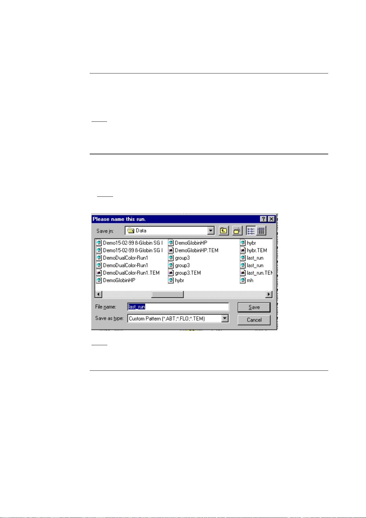
Create a Run Data File

• After you click on the Run button, a dialog box (shown below) will open and prompt you to name the file where the run data will be stored.

• Enter a name for the run data file and click the Save button. Note: To close the dialog box without specifying a file name, click on the Cancel button.

Note: After you save the data run file and the dialog box closes, the Loading Screen will appear and the software will prompt you to enter sample data for

the current run (see next page).

Continued on next page

B 26

2.1.4.2. Naming Samples at the Beginning of a Run, Continued

Loading Screen that Appears at the Beginning of a Run

After you click on the RUN button in the Experiment / RUN / EXIT Window, the Loading Screen (shown below) will appear. The software will prompt you to enter sample data for this run in the Sample Data table. Note: Start entering data for rotor position #1 and continue through the last rotor position that contains samples, including any gaps in the sample order.

Fields in Sample Data Table

To define sample data for the current run, describe your samples in these fields of the Sample Data table:

This field Contains this sample data

Rotor Position Indicates the position of the sample in the 32-sample

carousel.

Sample Name Lists the name of the sample as it will appear in the

sample loading dialog and the analysis results.

Type Indicates whether a sample is a positive control, negative

control, quantification standard, or an unknown.

Replicate of Indicates whether a sample is a replicate of another

sample located at another position in the carousel. Note: Enter the carousel position of the replicated sample.

Concentration Lists the concentration of a sample if it is known, e.g. if

the sample is a quantification standard.

Notes Allows additional sample information to be included.

Continued on next page

B 27

2.1.4.2. Naming Samples at the Beginning of a Run, Continued

Additional Fields on This Loading Screen

After entering the sample description into the fields of the Sample Data table, enter additional sample information into three fields along the bottom of the Loading Screen:

Field Location Contains this information

Temperature

Number of Samples

Left lower corner of Loading Screen

Lists the temperature that the sample chamber holds during the “Seek Process” at the beginning of a run. As a default during editing the sample list the LightCycler holds a temperature of 30°C.

Concentration Units

Right lower corner of Loading Screen

Note: This information is only used to correctly label the axis of the analysis program. It has no relevance for calculation of data as such.

B 28

2.1.4.2. Naming Samples at the Beginning of a Run, Continued

Additional Functions on This Loading Screen

This Loading Screen contains four buttons that perform the following useful functions:

Use this button To do the following

Done Closes the Loading Screen and opens the Run

Screen. Note: The instrument will begin to search for the indicated number of samples.

Enter Samples Later Allows user to define sample data after the

beginning of the run. Note: The Edit Samples button on the Run Screen

will flash red as a reminder that sample data still must be entered.

Clear Sample List Makes all fields in the Sample Data table blank. Default Sample List To reset the values in the Sample Data table to

values previously defined and stored in the *.exp- file by the user.

B 29

2.1.5. Real Time Fluorimeter (RTF)

Introduction The Real Time Fluorimeter (RTF) permits continuous monitoring of

fluorescence, even when a cycle program is not running. Whenever you set up a new experiment, e.g. with new primers, nucleic acid

templates, or with a new detection format, use the RTF to optimize the measuring sensitivity of the LightCycler fluorimeter. For example, you may adjust the fluorimeter gains to optimize the fluorescence response to variations in temperature or illumination.

Real Time Fluorimeter (RTF) Screen

From the Programming Screen, click on the Real Time Fluorimeter button. The RTF screen will appear (as in the photo below)

RTF Data Display

The graph that will appear on the gridlines of the RTF screen shows temperature and fluorescence output of a sample over time. The Real Time

Fluorimeter reads the raw output from the fluorimeters, so fluorescence outputs are plotted in tenths of a volt (i.e. a reading of 67 units equals 6.7 volts). Time is measured in seconds. Note: You may adjust the scale on the temperature axis by selecting the upper limit on the graph and typing in a new upper limit value. You may use the scroll bar at the bottom of the screen to move the display back and forth along the time axis.

Continued on next page

B 30

2.1.5. Real Time Fluorimeter (RTF), Continued

RTF Settings Use the fields at the bottom of the RTF screen to enter all RTF settings

described below. Fields are listed as they appear on screen from left to right.

Use this field... To alter this value

Target Temp.

Gains

Changes the temperature in the thermal chamber. The current temperature in the thermal chamber is displayed in the Value field to the left of Target Temp.

Note: To adjust the temperature, you may either type in a value, or adjust the value in the window incrementally by clicking on the small arrow tabs.

Caution: You must press Enter on the keyboard after typing in a temperature. Changes the enhancement factors in the fluorescence measuring channels. The range is 1-256. The default setting is 1, 15 and 30 for the respective channels F1, F2 and F3. Each channel can be individually switched on and off by clicking on the colored On/Off radio button to the left of the Gains field.

LED

Calibrated

Seek Sample

Note: As in other data screens, Channel 1 (F1) is optimized to detect emissions from SYBR Green I. Channel 2 (F2) is optimized to detect emissions from LC-Red 640. Channel 3 (F3) is optimized to detect emissions from LC-Red 705. The colored lines in the left lower corner of the screen show the color in which each parameter is displayed on the graph. Turns the LED light source on and off. The numerical value below the switch indicates the current LED level on a scale of 0-100%

Note: . We recommend using Calibrated LED only. If the Calibrated box is checked, the LED power is at 75% and cannot be adjusted Determines the power of the LED.

Note: We recommend leaving the LED power at its normal setting by leaving the Calibrated box checked x. If you would like to change the power setting, click on the x to clear the box; a scroll box will appear which allows you to make the necessary changes. When accessing the RTF, the LightCycler will seek sample #1. Enter the number of sample you wish to be graphed in the data display. Click on the Seek Sample button and the LightCycler will move the indicated sample into the optimal measuring position and acquire any other fluorescence signal of that sample.

Continued on next page

B 31

2.1.5. Real Time Fluorimeter (RTF), Continued

Finding the Optimum Gain Setting

To find the optimum gain setting for your experiment, proceed as described below:

Step Action

1 Prepare a capillary containing a complete PCR reaction mixture.

Note: As template, use the highest starting nucleic acid concentration that you plan to use in your experiment.

3 Depending on the detection format you plan to use, enter the

4 Verify that the correct measuring channel is turned on (i.e., the

5 6

• Place the capillary into the carousel.

• Load the rotor into the LightCycler.

temperature at which the fluorescence will be acquired during your experiment. Example: For SYBR Green I format, set the temperature at 72°C (temperature at end of extension phase). For Hybridization Probes format, set the temperature at the annealing temperature of the probes (usually in the range of 50°-60°C, at the end of annealing phase).

correct LED is lit). Note: Click on the F1 button for SYBR Green I; F2 button for Hybridization Probes. Click on the Seek Sample button to bring the capillary into the focus of the fluorimeter.

Adjust the fluorimeter Gain (by clicking on the small arrow tabs) until the displayed fluorescence signal is between 10 and 20. Caution: Gain values determined in the RTF will not be saved automatically when you exit the RTF and return to the Programming or Front Screen. However when returning to the Programming Screen you will be asked to confirm whether you wish to use the settings, chosen in the RTF in your experiment.

Exit RTF To quit the RTF and return to the Programming Screen or Front Screen,

either click on the Exit RTF button or choose “Exit RTF” from the File menu.

B 32

2.1.6. Programming Screen: Color Compensation Window

Location of Window

Color Compensation Window

Function of Color Compensation Window

The Color Compensation Window is in the upper left corner of the Programming Screen.

The Color Compensation Window allows you to select a software file (*.ccc file) containing information which can improve the display of data obtained with multicolor analysis systems (e.g., Dual Color Detection experiments). The use of color compensation is restricted to Hybridization probes. The DNA binding dye SYBR Green I is analyzed in channel 1 with no color compensation. Color compensation is also not required when a single color detection with LC Red 640 or LC Red 705 is performed. Note: See Section 5 of Chapter D for an example of a system that uses color compensation files.

How to Load a ccc File

If you select a *.ccc-file in the Color Compensation Window, color compensated run data will be displayed during a PCR run. To view the effect of color compensation during a run, do the following:

Step Action

1 2

Note:

• You may also choose and/or disable and enable Color compensation during

a Run.

• When Color Compensation is chosen, the Color Compensation file content

will be stored as part of the data-file, generated during the a Run.

• The Display of Fluorescence History however will not switch the displayed

fluorescence values back to the uncorrected values if you turn color compensation off. Data will be stored without color compensation after the run.

In the Programming Screen, open the *.exp-file (i.e., file name.exp). In the Color Compensation Window, click on “Choose CCC File” and select the appropriate color compensation file from the Calibration directory window. Color Compensation is automatically enabled. Click on Use Color Compensation to disable Color Compensation.

B 33

2.1.6. Programming Screen: Color Compensation Window,

Continued

Use of *.ccc Files for Data Analysis

In addition to using a *.ccc-file to generate a color compensated run display, you can use the file to analyze multicolor experiments more accurately. This important use of *.ccc-files is described more fully in Section 4.3.3 of this chapter.

B 34

2.1.7. Programming Screen: Display Mode / Fluorimeter Gains Window

Location of Window

Display Mode / Fluorimeter Gains Window

Display Mode

The Display Mode / Fluorimeter Gains Window is in the upper center portion of the Programming Screen.

To select the fluorescence display used during LightCycler runs, use the pulldown menus in the Display Mode window. One menu sets the numerator of the selection; the second sets the denominator of the selection. Choices for numerator and denominator include F1, F2, F3, and 1.

Note: The F1 channel is optimized to detect emissions from SYBR Green I or fluorescein, at wavelengths around 530 nm. The F2 channel detects emissions from LC-Red 640. The F3 channel is optimized to detect emissions from LCRed 705 (see Section 1.3.2 of Chapter C).

Examples: Use the following settings for typical experiments:

• For quantification runs with SYBR Green I alone, select F1/1.

• If fluorescein is used alone, select F1/1.

• If fluorescein is used with another fluorophore as a FRET pair (see Section

1.3.2 of Chapter C), select either F2/1 or F3/F1, depending on whether the second fluorophore is LC-Red 640 (F2/1) or LC-Red 705 (F3/F1).

Note: Channel Settings may also be selected and altered during a Run. For more information on the use of these fluorescence display settings in various applications, see Chapter D.

Continued on next page

B 35

2.1.7. Programming Screen: Display Mode / Fluorimeter Gains Window, Continued

Fluorimeter Gains

Different applications require different detection sensitivity. Use the Fluorimeter Gains window to set the correct detection sensitivity for your application in each of the fluorimeter channels. The gains may be adjusted on a scale from 1 to 256. You may either type in a gain number or click on the small tabs to adjust the number gradually. The default setting is 1, 15 and 30 for the respective channels F1, F2 and F3.

Note: Grain Settings cannot be changed during a Run, but must be set to their optimum values as described earlier. To determine the correct gain experimentally, use the Real Time Fluorimeter (RTF) (see Section 2.1.5 of this Chapter). If the signal for a channel in the RTF is too high, select a lower gain number. If the signal level is too low, select a higher gain number.

B 36

2.1.8. Programming Screen: Cycle Program Data and Temperature Targets Window

Location of Window

Cycle Program Data and Temperature Targets Window

The Cycle Program Data and Temperature Targets Window is in the center portion of the Programming Screen.

Cycle Program Data

The Cycle Program Data section automatically appears when a new cycle program is added to a protocol (e.g. by clicking the Add button under the Cycle Programs list as described in Section 2.1.2 above).The section accepts the following information:

Part Option

Cycles Field

Analysis Mode

Note: Information entered in this window is automatically saved without onscreen confirmation.

Type in the number of cycles to be run with the cycle program parameters to be defined in the Temperature Targets Window. Depending on the application and the cycle program, use the pull down menu to select the correct analysis mode:

• None,

• Quantification, or

• Melting Curves.

Note: The default setting is None. Change the setting if the data acquired during the cycle program is to be used for quantification or melting curve analysis.

Continued on next page

B 37

2.1.8. Programming Screen: Cycle Program Data and Temperature Targets Window, Continued

Temperature Targets

Field Description

Field Purpose

Target

Temperature

(°C)

Incubation Time

(h:min:s)

Temperature

Transition Rate

(°C/s)

Use the Temperature Targets section to define the temperature profiles for each individual program. Type the appropriate settings in the horizontal fields between the Ins and the Del buttons. Each temperature segment is inserted or deleted as follows:

Button Click on the button...

Ins

(Green)

Del

To enter a new temperature segment or to add a temperature segment in a new position. To delete a temperature segment.

(Red)

Enter the following information into the fields in the Temperature Targets section:

Defines the temperature of the segment in °C, e.g., 94°C for denaturation or 72°C for elongation phase.

Defines the holding time of a temperature segment. Use the following guidelines for setting typical incubation times:

• For denaturation: 0 s

• For annealing with SYBR Green I: 0–10 s

• For annealing with hybridization probes: 0–15 s

• For elongation: As a general rule, divide the length of fragment in bp

by 25 to determine the incubation time (in seconds). Note: If you enter a single number, it indicates the time is in seconds. To enter a time in minutes, you have to use a colon to separate minutes and seconds, e.g. ”10:30” means 10 minutes and 30 seconds. When entering 60 seconds or more "seconds" when leaving this field an automatic conversion from seconds to minutes occurs (e.g. 100 seconds will be converted to "1:40"). Defines rates at which the instrument changes temperature between temperature targets. The slowest rate is 0.1°C/s and the fastest rate is 20°C/s. Note: A fast transition rate (20°C/s) works well for amplification programs. Slower rates (0.1–0.2 °C/s) are recommended for melting curves.

Continued on next page

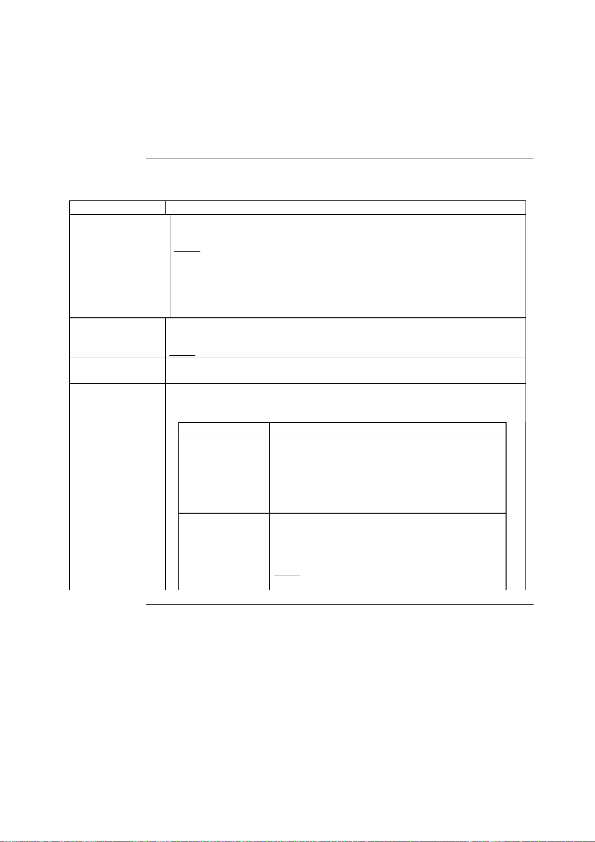
B 38

2.1.8. Programming Screen: Cycle Program Data and Temperature Targets Window, Continued

Field Description (continued)

Field Purpose

Secondary Target

Temperature

(°C)

Step Size

(°C)

Step Delay

(cycles)

Acquisition Mode

Defines a second target temperature within a segment beginning at a defined cycle number (see Step Delay below). Note: This is suitable for a so-called ”touch down” PCR. Here, annealing occurs at the upper temperature limit to ensure specificity during the first 15-20 cycles. However, this reduces the efficiency of amplification. After 15-20 cycles, the annealing temperature is decreased by as much as 10°C to the Secondary Target Temperature where annealing occurs

with lower specificity to facilitate greater amplification efficiency. Defines the degree change per cycle used to step up/step down from the Target Temperature to the Secondary Target Temperature. Note: A decrease of 1°C/cycle is commonly used in ”touch down” PCR. Defines the cycle number at which the step up/step down from the Target Temperature to the Secondary Target Temperature begins. Defines the time in each PCR cycle at which fluorescence measurement of samples is made. The available choices are:

None

Single Measures fluorescence once at the end of the

Cont.

(continuous)

No fluorescence measurement. temperature segment selected. For the

Hybridization Probe format, measurement occurs at the end of annealing phase; for the SYBR Green I format, it occurs at the end of the elongation phase. Monitors fluorescence data continuously from the first sample to the last one. The temperature continues to increase during measurement. Note: This acquisition mode is suitable for melting curve analysis.

Continued on next page

B 39

2.1.8. Programming Screen: Cycle Program Data and Temperature Targets Window, Continued

Field Description (continued)

Field Purpose

Acquisition mode

(continued)

Step

(stepwise)

Measures fluorescence at each temperature transition. Example: If you use Step to acquire fluorescence during a melting curve analysis, enter 0.2oC/s as your Temperature Transition Rate. The system will heat up the samples by

0.2°C, hold the temperature and measure all samples. It will then stepwise increase the temperature by 0.2°C and measure at the respective temperatures. Note: This acquisition mode is suitable for melting curve analysis.

B 40

2.1.9. Programming Screen: Graphic Simulation Window

Location of Window

Graphic Simulation Window

Cycle Program Simulation

The Graphic Simulation window is just below the Cycle Program list on the right side of the Programming Screen.

Click on the Simulation button in the Graphic Simulation window to display the Cycle Program Simulation. This simulation shows a graph of a single cycle of the program named in the Cycle Program list (directly above the window). Use this visual aid to confirm your cycling parameters

Experimental Notes

Note: In the simulation, the temperature profile is displayed as a red line, while the fluorescence acquisition profile is graphed in green.

In addition to the Cycle Program Simulation display, the Graphic Simulation Window can display notes about the current program. Use the buttons beneath the window to do the following:

Use this button To do this

Experimental Notes Edit Exp. Notes

Display notes on the program highlighted in the Cycle Program list. Alter the notes displayed in the window.

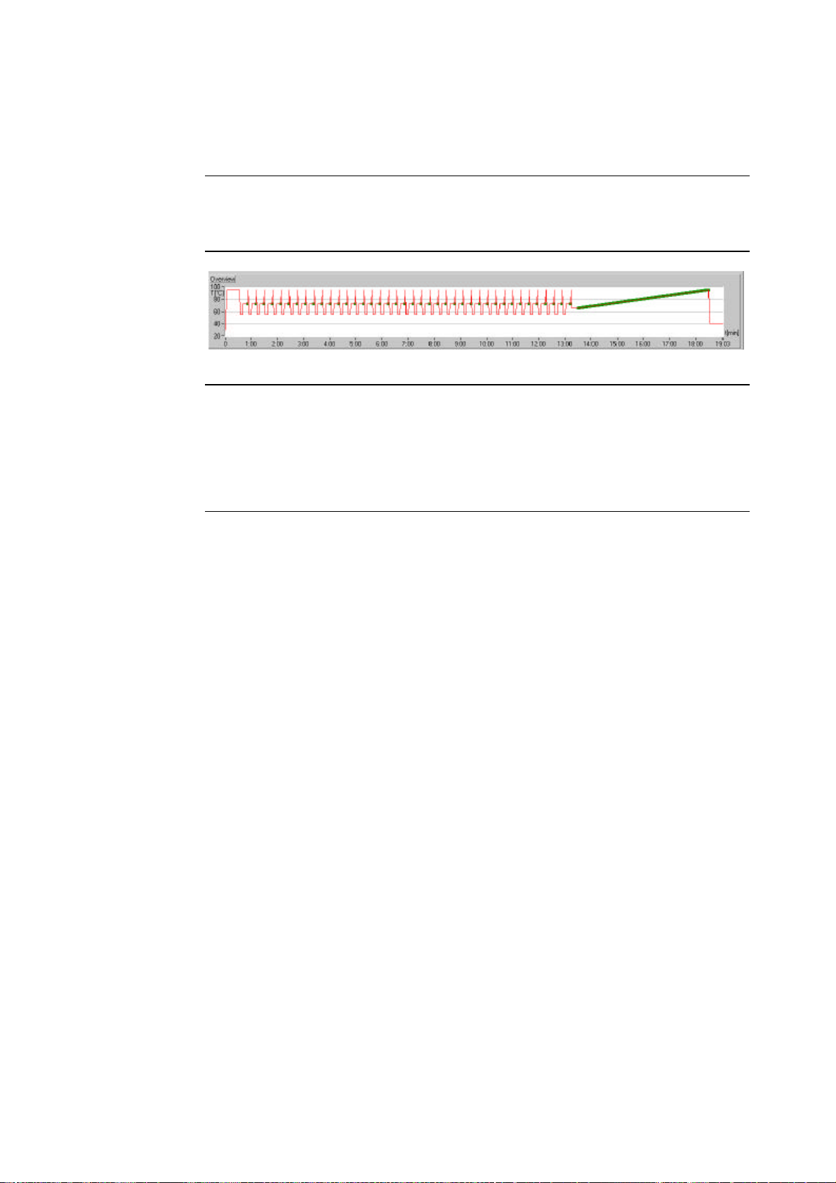
B 41

2.1.10. Programming Screen: Cycle Program Overview Window

Location of Window

Cycle Program Overview Window

Temperature Profile vs. Time

The Cycle Program Overview window stretches across the bottom of the Programming Screen.

The Cycle Program Overview window displays a graph of the current experimental protocol. The temperature profile is graphed in red, while the fluorescence acquisition profile is graphed in green. The time for the programmed Experimental Protocol is indicated as rough estimate.

B 42

3. Running the LightCycler

3.1. LightCycler Run Screen

Introduction When a PCR run is started, the monitor switches from the Programming

Screen to the Run Screen. This screen displays actual fluorescence values, the

development of fluorescence during the run, and the actual temperature online.

Note: A picture of the Run Screen is shown on the next page.

Run Screen Display

After the instrument detects the samples, temperature cycling begins and the Run Screen will display three graphs:

• Fluorescence vs. Time (Fluorescence History)

• Temperature vs. Time (Temperature History)

• Relative fluorescence of each sample (Current Fluorescence bar graph).

The screen also displays the following:

• Cycle Program Name

• Cycle Program Segment

• Cycle Number (currently in progress)

• Current Fluorescence Display Mode.

• Samples Names (and the corresponding line color used to display the

progress of that sample).

Note: If the LightCycler is unable to detect one or more samples, a dialog box will tell the user how many samples were found at which position and offer a chance to abort the run or continue it. This behavior also applies, when intentionally one position of the sample carousel was left free. In case the system was not able to find a capillary, repeat the seek with "Use Seek Threshold" disabled in the Options pull-down of the Programming Screen. Position #1 is always measured. Here, if no capillary is found, a default position, determined during instrument calibration is used.

Continued on next page

B 43

3.1. LightCycler Run Screen, Continued

LightCycler Run Screen

Fluorimetry Controls

A panel at the top of the Run Screen controls several fluorimetry display and acquisition (measurement) parameters.

Area Function

CCC File (fields) Display Mode

(pull down menus)

Fluorimeter Gains

(fields)

If you are using a color compensation file, this area will list the name of that file.

May be used to select the fluorescence channel(s) displayed during LightCycler runs. Note: Display mode is usually specified during programming (see Section 2.1.7 above), but may be changed here. Displays the detection sensitivity in each of the fluorimeter channels. Note: Gains cannot be changed during a run. Gains are set during the programming phase of the experiment (see Section 2.1.7 above).

Continued on next page

B 44

3.1. LightCycler Run Screen, Continued

Program Name / Segment / Cycle Number

Sample Names/ Default Colors

Other Buttons

The right section of the top panel shows 1) the name of the program (e.g. PCR, Annealing), 2) the number of the temperature segment now in progress, and 3) the number of the cycle now in progress.

A window in the far right corner of the screen lists 1) the names of the samples in the current run, 2) the rotor position of each sample, and 3) the color of the line (or bar) that represents each sample in the graphs.

Note: You can change the color coding by just clicking on the color squares to the left of the samples. Changes are effective in the current run and shall not be forwarded to the Graphics Defaults settings.To reset the color defaults that you defined earlier (see Section 1.5 above), click on the Default Colors button (lower right corner of the screen). This does not affect data display in the LCDA module.

In the lower right corner of the screen, there is a set of buttons. Use these buttons to perform the following functions:

Click on this

button...

End Program

Add 10 Cycles

Exit Run

Stop the cycle program that is currently running and move onto the next cycle program. Note: If the current program is the last in the protocol, clicking this button will return you to the Front Screen. Add ten more cycles to the program in progress. Note: Use this button if your amplification reaction is not complete or your reaction is proceeding slowly. This change is only effective for the current run and shall not be stored in the *.exp-file. End the run immediately and offer you two options:

• Save, or

• Cancel.

Note: If there was an error in the program or you do not want to save the data click on Cancel. Otherwise, click on Save to save the run data for later analysis. Caution: If a protocol is run twice, both sets of data cannot be saved. You can replace the first set of data with the second set, rename the second data set, or hit

Cancel to save the original data.

To do this...

Continued on next page

B 45

3.1. LightCycler Run Screen, Continued

End of Run

• If the LightCycler completes a run, it will automatically save the program.

• After the LightCycler finishes a run, it will automatically open a data

analysis window that displays the data acquired in the current run.

Note: When at the end of a Run another experiment is being analyzed, the current data will not be displayed atomatically.

B 46

4.1. Introduction

4. Data Analysis

Starting Data Analysis

Analysis Formats

Format Select by clicking Description

Quantification

Melting Curve

To begin data analysis, do either of the following:

• Simply allow the LightCycler to complete a run. When the protocol has finished, the software will automatically display the collected data on the LightCycler Data Analysis (LCDA) Front Screen.

• If no run has been performed, open the LCDA Front Screen by clicking on the Data Analysis button on the LightCycler Front Screen.

The LightCycler Data Analysis (LCDA) software allows a LightCycler user to analyze quantification data or melting curve data acquired during a LightCycler reaction. The LCDA software can display and analyze data in two formats:

Quantification button (at top of screen)

Melting Curve button (at top of screen)

Estimates the original number of target DNA copies in a sample by comparing it to at least two known concentrations of a standard. It displays the amplification profile of a PCR. Displays a fluorescence curve profile obtained during a slow denaturation of PCR products, and includes options for differentiating melting curves to give melting peaks, integrating the area under the melting peaks, and defining the melting temperature of amplified products.

In this Section

Note: You must select the segment of the run to be analyzed and define other analysis parameters before the data can be analyzed. For more information, see the following sections of this chapter for details:

• See Section 5 for details on defining parameters for the Quantification format, including setting the baseline and crossing line, determining crossing points, and selecting data from a set of standards to generate a standard curve.

• See Section 6 for details on defining parameters for the Melting Points format, which are similar to those used for the Quantification format.

The rest of Section 4 gives a brief overview of the various parts of the LCDA Front Screen. See Sections 5 and 6 for detailed information on using these parts to set up a Quantification or Melting Curve analysis.

B 47

4.2. Select Data File / Data Analysis Window

Select Data File to Analyze

Searching for a Data File

You must choose the data to be analyzed by doing the following:

• Select “Open” from the File menu on the LCDA Front Screen. A Data Analysis Window (shown below) will open and display a list of LightCycler data files. For each file, the list gives the File Name, User Name, date / time Created, and date / time Analyzed

Note: You will see only those files that belong to the current user (e.g., the user whose log on name was used to enter the LightCycler software. Every user has an individual data folder.

• Use the pointer to highlight the file containing the data.

• Click on the Open button.

Result: The LCDA Front Screen will open and display the selected data file in a new window.

Note: A new window is created for each open file. Thus, you may open and analyze several data sets by moving between windows.

If you are not certain which data file you want, you may use the fields at the bottom of the Data Analysis Window to search for a select subset of files. These fields allow you to search for files by File name, User name, Date

Created or Date Analyzed.

Data Analysis Window

Continued on next page

B 48

4.2. Select Data File / Data Analysis Window, Continued

Additional Information on Data Files

File Open Default Settings

After a file is highlighted (but before it is opened), additional information about the file will be displayed in the box at the right of the Data Analysis Window. This information includes:

• File name

• Number of linked programs that constitute the run, with a brief description

of each program

• Number of samples

• List of all sample names.

Note: If the samples were designated as standards of known concentration, the concentrations will also be listed next to the sample name.

The Preferences option under the pull down "Help" menu of the LCDA Front screen allows customizing the file open default settings.

Select by Clicking Description

Initial Directory Allows the user to define the directory from

which he wants to start in when the open file dialog appears for the first time.

Export Data Allows the user to define the format of numbers

when data will be exported.

B 49

4.3. LCDA Front Screen

Introduction When you open a data file from the Data Analysis Window, the data will

automatically be displayed in the LCDA Front Screen shown below. The data will eventually be displayed in two sections of the window:

• Initially, the top section of the window will display the run data as a Temperature versus Time graph. On this graph, you must define the section of the run that will be analyzed by bracketing the selected section with the green cursors (see Section 4.3.1).

• After you set the cursors, the lower section of the window will display the fluorescence data acquired during the selected section of the run (as shown below).

Note: In this and all subsequent data analysis screens, you can enlarge or reduce the size of each graph by clicking on the horizontal divider between the graphs and moving it up or down.

LCDA Front Screen

Continued on next page

B 50

4.3.1. LCDA Front Screen: Temperature vs. Time Graph

Set Cursors for Quantification Analysis

To use Quantification analysis to analyze the data (i.e., data acquired once per cycle), set the green cursors to bracket the section of the graph that represents the amplification program (as shown in the photo below).

Note: To automatically bracket an amplification program, click the Select a Program button and then select the program segment in which amplification

took place. (For example, see the upper left corner in the picture of the LCDA Front Screen on the previous page. The name of the selected segment appears in the window below the Select a Program button.) To further refine the data to be analyzed grab and move the green cursors manually.

Set Cursors for Melting Curve Analysis

To analyze melting curve data (i.e., data acquired continuously), set the green cursors to bracket the section of the graph that represents the melt program (as shown in the photo below).

Note: To automatically bracket a melt program, click the Select a Program button and then select the program segment of the protocol in which melting took place. To further refine the data to be analyzed grab and move the green cursors manually.

Continued on next page

B 51

4.3.1. LCDA Front Screen: Temperature vs. Time Graph, Continued

Upper Graph: Temperature vs. Time

Change Graph Settings

The graph in the top section of the LCDA Front Screen displays the temperature cycles (black line) during the run, as well as the temperatures at which fluorescent data was acquired (pink line). To define the area of this graph that will be analyzed, do one of the following:

• Use the mouse to move the green cursors until they bracket the area to be analyzed.

• Click on the button at the left corner of the graph to open a window (as shown below). In this window, you may enter a number in the Value field to specify the position of each cursor (expressed as a particular time, in h:min:s format). After you have entered the times for each cursor, click the OK button to set the cursors.

To change any axis values of the graphs displayed click on the button on the top left corner of the graph.

This will bring up a Customize Graph screen. In this screen the user can define values for the axis which will then be carried into the LCDA display. Deselect the Automatic Fit option and enter values for the axis in the appropriate fields.

B 52

4.3.2. Fluorescence vs. Cycle Number / Time / Temperature Graph

Fluorescence vs. Cycle Number

Select x-Axis

After you set the cursors in the top graph (see Section 4.3.1 above), the bottom graph (as shown in the photo below) will display the fluorescence data acquired during the bracketed section of the protocol.

In the pull down menu below the bottom graph, you may select any of three options for the parameter plotted on the x-axis: Time, Temperature, or

Cycles. Use the following guidelines to select the appropriate parameter:

If you will analyze... Then select...

Fluorescence data acquired once per cycle (i.e., quantification data) Fluorescence data from a melt Any experiment (default setting, for data viewing only)

Cycles

Temperature

Time

Continued on next page

B 53

4.3.2. Fluorescence vs. Cycle Number / Time / Temperature Graph, Continued

Select Fluorescence Display

Guidelines for Fluorescence Display

To set the fluorescence channel to be displayed in the lower graph, highlight the appropriate item in the pull-down menu to the right of the y-axis. You may choose to display fluorescence data from a single channel (F1, F2, or F3) or a ratio of data from two channels (F1/F2, F1/F3, F2/F1, F2/F3, F3/F1, or F3/F2).

Use the following guidelines to determine which fluorescence display to use for various applications:

Use this fluorescence display... For assays containing...

F2/F1

F3,

F3/F1

• SYBR Green 1

• Fluorescein

• LC-Red 640

• LC-Red 640 / Fluorescein

Hybridization probe pair

• LC-Red 705

• LC-Red 705 / Fluorescein

Hybridization probe pair

Note: When opening a file the first program with data acquisition is bracketed and the channel setting is chosen in the *.exp-file selected.

Example: For examples of experiments which use different fluorescence display settings, see the applications described in Chapter D.

B 54

4.3.3. LCDA Front Screen: Using Color Compensation Files

Color Compensation

Preparing a Color Compensation File

Saving a Color Compensation File

The following dyes can be used for multicolor analysis with the LightCycler:

Analysis Format Channel 1 Channel 2 Channel 3

Hybridization Probes

Each of the fluorophores listed above has a different emission maximum, and the LightCycler detection filters have been optimized to these maxima. However, when more than one of these dyes is used in a single run, there is some crosstalk between fluorimeter channels. LCDA color compensation software compensates for this between-channel crosstalk.

To use color compensation, you must first create a *.ccc (ccc)-file in a calibration experiment with the dyes listed above (see Section 5 of Chapter D for details). Note: We offer a LightCycler Color Compensation Set (Cat No. 2 158 580), with ready-to-use solutions and optimized conditions for the generation of ccc files.

After completing a calibration run, do the following:

Fluorescein LC Red 640 LC Red 705

Step Action

1 Open the acquired data in the Programming Screen. 2

3 4 Save the color compensation data by naming the calibration file.

Note: Once you have created and saved a color compensation calibration file, you can use that data to correct many future data sets (as long as you use the same combination of fluorophors).

In the Select a Program pull-down menu in LCDA, highlight the program segment that includes the melting program. From the Color Compensation menu, select “Calibration”.

Note: The file name must end in “.ccc”, e.g. data1.ccc.

Continued on next page

B 55

4.3.3. LCDA Front Screen: Using Color Compensation Files,

Continued

Using a Color Compensation File During Data Analysis

To use a calibration file to color compensate run data, follow the steps described below:

Step Action

2 3 Under the Color Compensation menu, select „Load Calibration

4 To see what your data looks like after color compensation, do

From the Data Analysis Window, open the file containing the run data (see Section 4.2 of this chapter). Result: The LCDA Front Screen will appear and display the run data. Bracket the program segment to be analyzed in the Temperature vs. Time screen (see Section 4.3.1 of this chapter).

Data“, and click on the name of the stored ccc (calibration) file. Note: You may also click on the Select CC Data button (top center portion of screen) to find the stored ccc file.

either of the following:

• Click on the Color Compensation button (top center portion of screen), or

• Select „Enable“ under the Color Compensation pull-down menu.

Click on the Color Compensation button again to return to the raw data.

B 56

4.4. LCDA Front Screen: Data Retrieval

Introduction

Print Data

You can retrieve permanent copies of the data displayed on the LCDA Front Screen. This section describes options for data retrieval.

You can print a hard copy of the data displayed on the screen. To print either the upper or lower graph:

• From the File pull-down menu, select “Print Window”, and

• On the Report pull-down menu, highlight the graph to be printed. The

Report function will launch the LightCycler Software report tool "Graphworks".

4.5. Further Analysis

Further Analysis of Amplification or Melting Curve Data

If you have collected data in specific formats, you can use the buttons at the top of the LCDA Front Screen to prepare them for further analysis, as follows:

If the data is displayed as... Fluorescence vs. Cycle

(e.g., fluorescence data that was acquired once per cycle)

Fluorsence vs. Temperature

(e.g., fluorescence data acquired continuously from a melting experiment)

For further analysis, click... Quantification button

Melting Curve button

And...

Use Section 5 of this chapter to set up a Quantification analysis

Use Section 6 of this chapter to set up a Melting Curve analysis

B 57

5. Display and Analysis of Quantification Data

5.1. Introduction

Quantification on the LightCycler

Fluorescence Acquisition for Quantification Analysis

Use of Crossing Line to Quantify Unknowns

The LightCycler performs a quantification analysis by comparing the fluorescence of a PCR product of unknown concentration with the fluorescence of several dilutions of an external standard. For this analysis, the instrument considers only fluorescence values measured in the log-linear phase of amplification.

Note: To perform a quantification analysis the user must have defined at least two standards of known concentration in the Loading Screen. Ideally, standards are amplified under the same conditions as the unknowns and have the same amplification efficiency. We recommend using the same primer set to amplify both standards and unknowns.

In order to quantify PCR product with the LightCycler, the instrument must be set up to acquire fluorescence once per cycle. This will generate a fluorescence curve that increases in value with each cycle as the product accumulates.

The most useful data occurs during the few cycles in which the fluorescence readings are above background and increase in a log-linear fashion. The LCDA quantification software is designed to generate a best-fit line from this log-linear region of each curve.

This best-fit line will be parallel to the x-axis and is called a Crossing Line. The point at which the Crossing Line intercepts the log-linear region of each fluorescence curve may be used to calculate the concentration of the sample that generated the fluorescence curve.

The instrument plots a standard curve of the Crossing Line intercepts of the standards vs. the known concentrations of these standards. By comparing the Crossing Line intercept of an unknown sample with the standard curve, the instrument generates a quantitative estimate of the starting copy number of the target DNA in the unknown.

B 58

5.2. Quantification: Selection of Analysis Method

Quantification Analysis Methods

Fit Points Method (Default Method)

Clicking on the Quantification button on the LCDA Front Screen will open the Quantification Analysis window. Once that window is open, the first step of the data analysis is to select the appropriate analysis method. There are two choices. The descriptions given below should help you determine the most suitable analysis.

Note: To choose either of the two methods, click on one of these buttons:

• Fit Points, or

• Second Derivative Maximum

Alternatively, you can choose either of the methods under “Analysis Method” in the Quantification menu. Note that the Fit Points option is called Fit N Points Above Threshold in this menu, while Second Derivative Maximum has the same name on both the menu and the button.

This method is possible with all applications. When quantitating samples containing low copy numbers of target DNA (typically less than 1000 copies), the Fit Points method often gives better results than Second Derivative Maximum. Fit Points also works well at high copy numbers, so if the template concentration in your samples ranges from low to high, you should use Fit Points. Additionally this method shows backward compatibility to the old software.

Second Derivative Maximum Method

Note: Set up and analysis by the Fit Points method requires three steps: Step 1: Baseline, Step 2: Noise Band and Step 3: Analysis. These steps are described in

detail in Sections 5.3–5.5 of this chapter.

The Second Derivative Maximum method is better for analyzing high copy numbers (above 1000 copies per tube) since it requires no user input or bias. However, this method may have problems analyzing low copy numbers that lead to less well-behaved reactions. The Second Derivative Maximum Method is a semiautomated method, that uses the shape of the curve to determine the target copy number. It is independent of user-borne influences and will produce identical data e.g. irrespective of baseline subtraction method.

Note: Set up and analysis by the Second Degree Maximum method requires only two steps: Step 1: Baseline, Step 2: Analysis. This method does not require setting a noise band (Step 2 under Fit Points above). See the next page for more information.

Continued on next page

B 59

5.2. Quantification: Selection of Analysis Method, Continued

Tabs on the Quantification Analysis Screen

The Quantification Analysis screen will display fluorescence curves for all the samples in the selected run. If you chose the Fit Points method, you will see three tabs displayed at the top of the screen: Step 1: Baseline, Step 2: Noise Band, and Step 3: Analysis. Note: For more details on each stage, see the section of this chapter listed in the table below). If you chose the Second Derivative Maximum method, you will see only two tabs: Step 1: Baseline and Step 2: Analysis.

To set up and perform the analysis, you must select each tab in turn, and define the appropriate data analysis parameters in the screen that appears. The following parameters must be defined:

Stage Description See

Section

Step 1:

Baseline

Step 2:

Noise Band

(Fit Points

method only)

Step 3:

Analysis

For valid comparison, all samples should have baseline fluorescence values close to zero. In this screen, you will define any baseline corrections that are necessary prior to analysis. In this screen, you will set the noise band that defines non-informative fluorescence data.Typically, this is data that cannot be distinguished from the fluorescence noise in the earlier cycles of amplification.

Note: Not required for the Second Derivative Maximum method. This method is a semiautomated approach to quantitative PCR. It solely interprets the shape of the curve to determine copy number. Consequently, it does not require setting a Noise Band, nor a Crossing Line. Also Baseline correction is solely performed to free the graph from effects of background variability. It will not have any effect on quantification as such.

In this screen, you will determine the point of intersection between the fluorescence curves and a defined crossing line. You will select the type of threshold setting from several options. Note: The values for the crossing points are used to generate a standard curve which plots Cycle Number vs. Log Concentration and this standard curve will be used to calculate concentrations for unknown samples.

5.3

5.4

5.5

Continued on next page

B 60

5.2. Quantification: Selection of Analysis Method, Continued

How to Use this Part of the Manual

Each of the steps in the table above are described more fully in Sections 5.2–

5.5 of this chapter. You may use these sections to familiarize yourself with the steps of a Quantification Analysis. After you are familiar with the required steps, use the convenient procedure (Section 5.6 of this chapter) to set up and perform Quantification Analysis.

B 61

5.3. Quantification Step 1: Baseline

Step 1: Baseline Screen

Continued on next page

B 62

5.3. Quantification Step 1: Baseline, Continued

Step 1: Baseline

Quantification

Regardless of which analysis method you choose, you must use the Baseline Screen to define any baseline corrections necessary for data analysis.

Note: Baseline fluorescence may vary from sample to sample for several reasons including differences in sample preparation, differences in DNA content from tube to tube or pipetting error. However, in order to make sample to sample comparisons easier, you must set the baseline fluorescence for all samples to zero. The Fluorescence vs. Cycle Number graph (shown on the previous page) has been carried over from the LCDA front screen and is used for baseline adjustment. As you select a method for baseline adjustment, this graph will change. The corrected graph will then be carried over to the next screen.

There are four options available for baseline adjustment:

Baseline

adjustment

None No baseline adjustment.

Arithmetic

(Default option)

Proportional

Recommended for any application with high sample-tosample background variation. In this method, the mean value of the five lowest measured data points for each sample will be calculated, then subtracted from each reading point in the sample. Note: This method is best for SYBR Green I reactions, since the template DNA will sometimes give a signal that is removed most efficiently by this method. When target DNA presents no baseline problem, the Proportional method can remove some of the tube-totube variations due to pipetting.

Description

Normalization

Note: This method is best for hybridization probes, TaqMan probes, Beacons, and especially suited for Dual Color experiments.

All fluorescence curves are displayed as a percent of maximum fluorescence. One hundred percent fluorescence is represented by the value 100. This brings all fluorescence curves to the same maximum value. When used with the Fit Points Method, it will alter the curves such, that incorrect quantification data may be produced. Note: This method is not suited for analysis.

Continued on next page

Roche LightCycler User manual

Specifications and Main Features

Frequently Asked Questions

User Manual

Prologue

Symbols and Notes

LightCycler Software and License Agreement

Chapter A

1. Technical Aspects of the LightCycler Instrument

1.1 Table of Contents

1.2 LightCycler System

1.3 Technical Data

1.3.1 Specifications of the LightCycler

1.3.2 Specifications for Applications

1.3.3 Specifications for the Detectors

1.3.4 Temperature Control

1.4 Safety Precautions for the LightCycler

2.1. The LightCycler

2. System Description

2.2 PC Configuration

3. Installation

3.1 Installation Requirements

3.2 Installation of the LightCycler

3.3 Installation of the Computer

3.4 Installation of LightCycler Software Version 3

3.5 Dismantling the LightCycler System

4. Operation and Maintenance of the LightCycler

Chapter B

1.1. Table of Contents

1. Software

1.2. Introduction

1.3. The Front Screen

1.4. Functions of Buttons on the Front Screen

1.5. Edit Graphics Defaults Window

2. Programming a Run

2.1. Programming Screen

2.1.1. Menu Options Available on the Programming Screen

2.1.2. Programming Screen: User / Experiment Window

2.1.3. Programming Screen: Experiment / RUN / EXIT Window

2.1.4. Programming Screen: Sample Data Entry

2.1.4.1. Loading Screen Activated by Edit Samples Button

2.1.4.2. Naming Samples at the Beginning of a Run

2.1.5. Real Time Fluorimeter (RTF)

2.1.6. Programming Screen: Color Compensation Window

2.1.7. Programming Screen: Display Mode / Fluorimeter Gains Window

2.1.8. Programming Screen: Cycle Program Data and Temperature Targets Window

2.1.9. Programming Screen: Graphic Simulation Window

2.1.10. Programming Screen: Cycle Program Overview Window

3. Running the LightCycler

3.1. LightCycler Run Screen

4.1. Introduction

4. Data Analysis

4.2. Select Data File / Data Analysis Window

4.3. LCDA Front Screen

4.3.1. LCDA Front Screen: Temperature vs. Time Graph

4.3.2. Fluorescence vs. Cycle Number / Time / Temperature Graph

4.3.3. LCDA Front Screen: Using Color Compensation Files

4.4. LCDA Front Screen: Data Retrieval

4.5. Further Analysis

5. Display and Analysis of Quantification Data

5.1. Introduction

5.2. Quantification: Selection of Analysis Method

5.3. Quantification Step 1: Baseline