

Page 1

NIS-Elements
M378 E 07.5.NF.5
Advanced Research
User’s Guide
(Ver. 2.34)
Page 2

Page 3

Thank you very much for choosing Nikon.
This manual explains installation and use of the NIS-Elements Advanced Research. For
trouble-free operation, read this manual before using the program.
No part of this manual may be reproduced without Nikon’s permission.
The content of this manual is subject to change without notice.
Nikon has carefully prepared this manual. However, we make no expressed or implied
warranty of any kind and assume no responsibility for such errors or omissions.
Be sure to read the instruction manuals for the microscope and PC you plan to use with the
NIS-Elements Advanced Research.
Trademarks:
Microsoft® and Windows® are either registered trademarks or trademarks of Microsoft
Corporation in the United States or other countries.
Products and brand names are trademarks or registered trademarks of their respective
companies.
The “TM” and ®marks are not used to identify registered trademarks and trademarks in this
manual.
To run NIS-Elements Advanced Research optimally, the following specifi cations are
recommended.
Recommended PC Environment:
CPU: Pentium IV, 3.2 GHz or faster
RAM: 1GB or higher
Operating system: Windows XP SP2 (English)
Hard disk space: 600MB of available hard disk space for installation
Display settings: 1280 x 1024 (True Color mode)
User rights: Administrators for installation and operation
*Operation cannot be guaranteed on all computer models. For futher information, contact
your nearest Nikon representatives.
Page 4

Page 5

Table of contents
INSTALLATION AND STARTUP
NIS-Elements Installation ................................................................7
APPLICATION APPEREANCE
NIS-Elements Screen .................................................................... 15
Layout Manager ......................................................................... 19
Organizer ................................................................................. 25
SETTING THE HARDWARE UP
Cameras .................................................................................. 33
Confi guring Attached Hardware ....................................................... 35
CAPTURING IMAGES
Images Capturing ........................................................................ 43
Time Lapse Acquisition ................................................................. 45
Multipoint acquisition .................................................................. 47
Z Series Acquisition ..................................................................... 49
Fluorescence acquisition ............................................................... 51
Capturing to Ring Buffer ............................................................... 53
DOCUMENTS, ARCHIVING
NIS-Elements Document Structure ................................................... 57
Working with Documents ............................................................... 61
IMAGE ANALYSIS
Histogram and Look Up Tables ........................................................ 67
Binary Editor ............................................................................. 73
Measurement ............................................................................ 77
Object Count ............................................................................ 81
Time Measurement ...................................................................... 85
Mathematical Morphology Basics ..................................................... 91
How to create a simple macro? ...................................................... 101
Creating Reports ....................................................................... 105
Page 6

CUSTOMIZATION
Modifying Main Toolbar ................................................................. 113
Command Line Options ................................................................. 117
ADDITIONAL MODULES
Database Module ........................................................................ 121
Extended Depth of Focus Module ..................................................... 131
ND Experiments ......................................................................... 137
Deconvolution Module .................................................................. 141
The 2D RT Deconvolution Module ..................................................... 143
Stage XY Module ......................................................................... 147
Stage Z Module .......................................................................... 157
90i Module................................................................................ 163
TE2000 Module .......................................................................... 167
Coolscope Module ...................................................................... 171
Nikon MM 400/800 Microscope ........................................................ 175
Nikon Eclipse LV Series Microscope ................................................... 179
Nikon AZ100 Microscope ............................................................... 187
Chapters and paragraphs marked by this symbol describe features available only in the
Advanced Research version of NIS-Elements.
Page 7

Installation and Startup
Page 8

Page 9
Installation
NIS-Elements Installation
Quick Start
The CD-ROM
Content
Installation
Quick Start
- Insert the installation CD in the CD-ROM drive. A splash screen automatically appears.
- Install the selected NIS-Elements software version, additional modules, and device
drivers.
- Plug in your HASP key into the USB port of your PC.
- Run NIS-Elements
The CD-ROM Content
The CD-ROM contains the NIS-Elements software itself, Windows system drivers for all
supported cameras, drivers and utilities for HASP, documentation in PDF format, a sample
image database, and sample image sequences for additional modules.
The installation process
Note that you have to possess the administrator rights to your computer to be able to install
NIS-Elements successfully. When the installation CD is inserted a splash screen appears.
Specifying
the software
version
Select the software version to be installed. Select the one you‘ve got the license for and that
is properly coded in your HASP hardlock key. The welcome dialog box appears. Click Next
to continue.
Page 7
Page 10
Installation
Installation
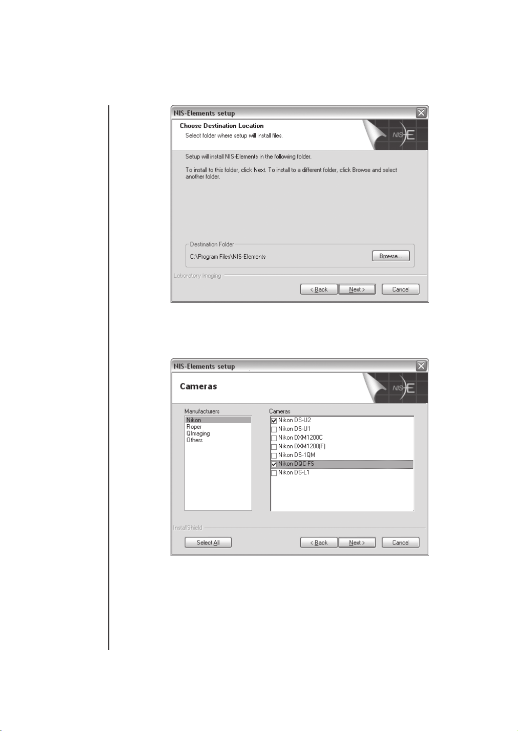
directory
Defi ne the folder where the NIS-Elements software should be installed. We recommend to
use the predefi ned directory. If you want to change the directory, press the Browse button
and select a new one, otherwise click Next .
Selecting
cameras
Now select the cameras you want to use with NIS-Elements.
Page 8
Page 11
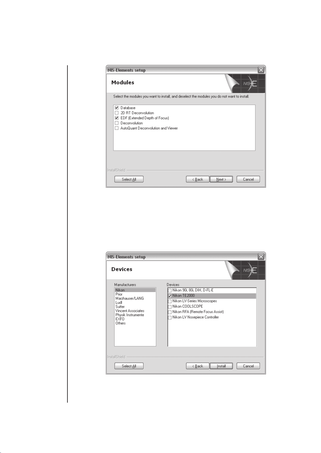
Selecting
modules
Installation
If your licence contains some additional modules besides the NIS-Elements base software,
please select them in this window.
Selecting
devices
Note:
Any module selected will be installed along with NIS-Elements automatically. However, you
might not be licensed to use it. The module will run after you get a corresponding code
registered in your HASP key.
Page 9
Page 12
Installation
If your licence contains some device controllers listed in this window, please select them.
Finish the installation by clicking the Install button.
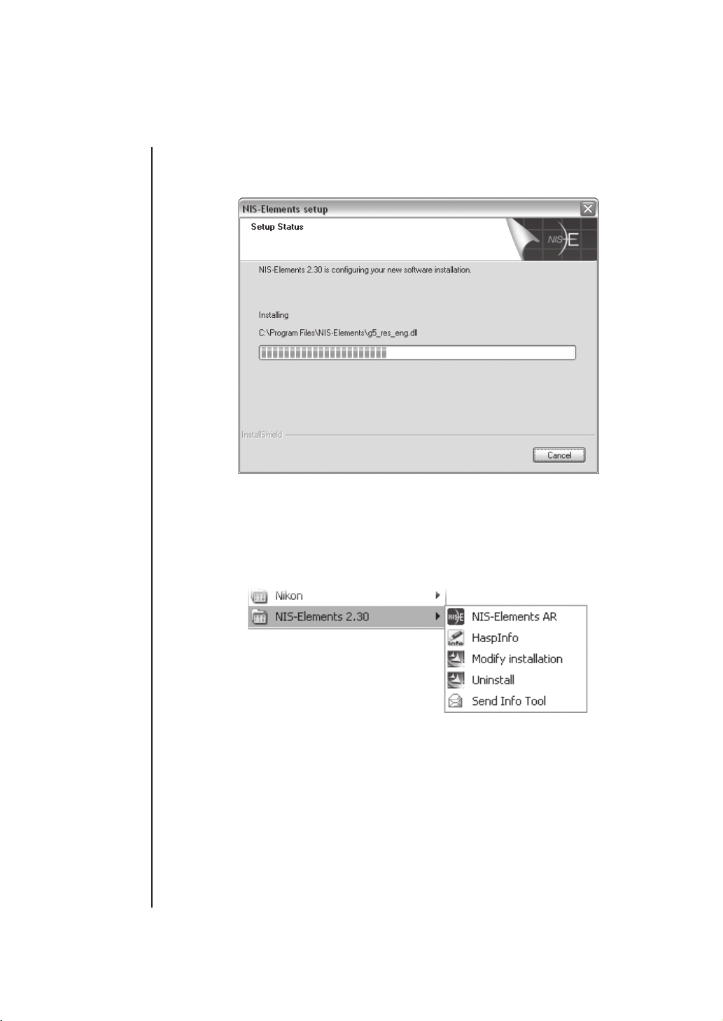
The program
group
Additional
installations
The Setup creates the NIS-Elements program group with the following items: HASP key information, NIS-Elements shortcut, Modify Installation (for adding hardware drivers, modules,
etc.), Uninstall procedure, and the Send Info Tool. A shortcut is created on the desktop. These
changes affect all user profi les of your local Windows system.
Note:
Clicking the Uninstall command deletes all installed fi les from disk, and removes the NIS-
Elements program group from Windows Start menu as well as the desktop icon.
Additional Module/Device installation
You may need to install a device or additional module after the NIS-Elements main system
installation.
Page 10
Page 13
Installation
- Go to Start menu>Programs>NIS-Elements program group.
- Select the Modify Installation command.
- Follow the install shield instructions.Check the checkboxes by the items you would like to
add.
- Finish the installation.
Installing sample database
Software copy
protection
Sample Database installation
If you chose to install the Sample Database, a new subdirectory „Databases“ is created
in NIS-Elements installation directory (e.g. C:\Program fi les\NIS-Elements\Databases\...).
The „Sample_Database.mdb“ fi le is copied in there along with database images (stored in
subdirectories). An administrator username/password to access this database is set to:
- Username: „sa“
- Password: „sa“
The software copy protection
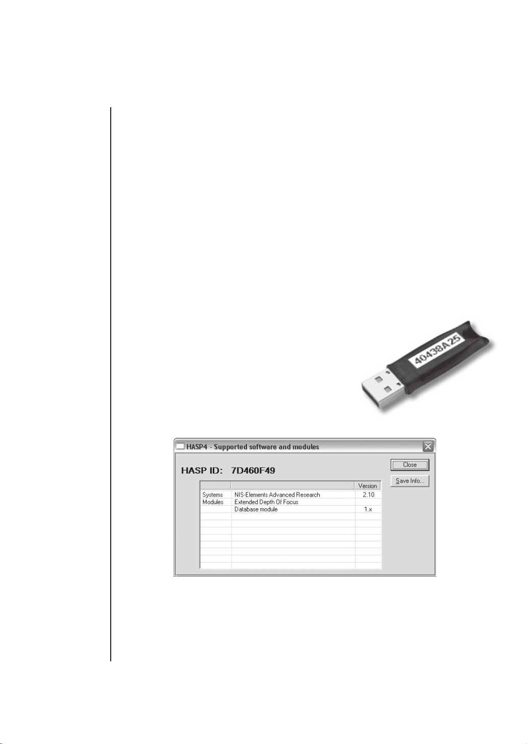
The NIS-Elements software is delivered with a HASP hardware key.
The HASP key contains information about the SW licence and allows
users to run the corresponding software. Please connect the
USB HASP after NIS-Elements installation. The utility called
„HASPinfo“ (Help menu) is installed to the NIS-Elements
directory. It enables the user to view information about
the actual software licence:
Page 11
Page 14

Installation
Page 12
Page 15

Application Appereance
Page 16

Page 17
NIS-Elements Screen
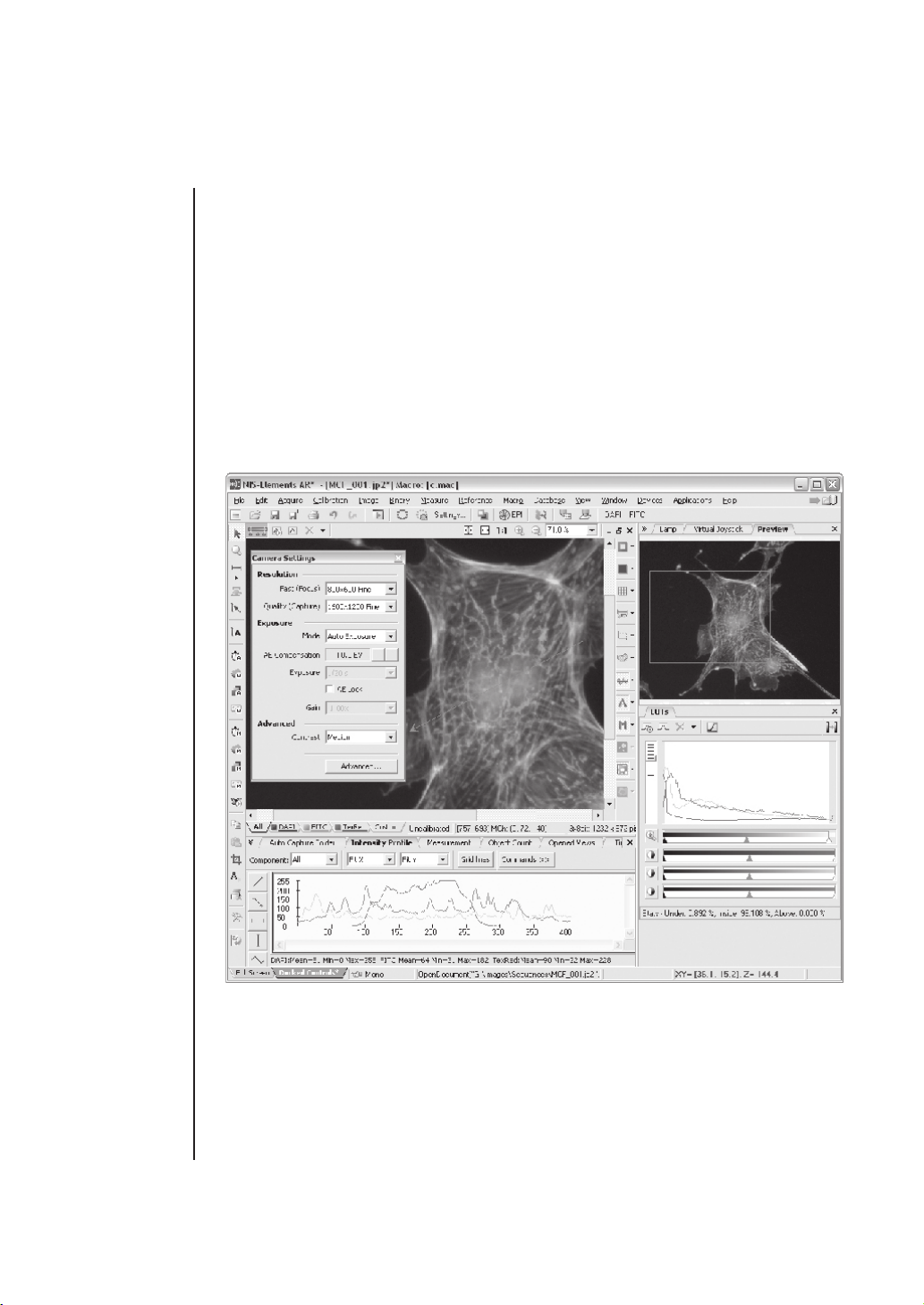
NIS-Elements Screen
Screen items
The following items appear on the screen:
- The menu bar containing pop-up menus with sets of commands.
- Two main toolbars (horizontal and vertical)
- Document toolbars (right and top) enabling to customize the images view. See its
description in the Document structure chapter.
- Docked control windows - see more description of docking windows in the Layout
Manager chapter.
- The status bar displaying useful information.
Page 15
Page 18

NIS-Elements Screen
Main toolbars
Horizontal toolbar
- Open fi le shortcut.
- Save fi le shortcut.
- Save Next shortcut.
- Print Image shortcut.
- Undo button.
- Redo button.
- Show live window displays a new document window with live signal from camera.
- RAM buffer ON - please see the Capturing to ring buffer chapter.
- Capture to RAM buffer - please see the Capturing to ring buffer chapter.
- Background correction ON is a shortcut to the Acquire>Backgroun Correction
ON/OFF command.
- Explore optical confi gurations button shows the optical confi gurations manager.
- New optical confi guration runs the optical confi guration wizard.
Vertical toolbar
- Pointing Tool enables to drag the image.
- Magnifi er Glass - interactive magnifi er tool to examine image details.
- Length measurement tool for interactive length measurements.
- Area measurement tool for interactive area measurements.
- Taxonomy tool for sorting objects in the picture into classes.
- Counts tool for counting objects in the picture.
- Radius tool for measuring radius of a circle.
- Semiaxis tool for measuring semiaxes of an ellipse.
- Angle tool for measuring angles.
- 3D Measurement tool measures length accross Z sequences (req. EDF module).
- Insert Arrow tool for inserting annotations.
- Insert Text tool for inserting text annotations.
- Capture Time Lapse automatically or manually.
- Capture Z Series automatically or manually.
- Capture Multichannel automatically or manually.
- Capture Multipoint automatically or manually.
- Real Time EDF performs Z series acquisition and EDF in one step (req. EDF)
- Copy copies the current image to memory.
- Paste As New Image creates a new document and inserts the image from memory.
- Crop tool for cropping images.
- Run Macro command runs the current macro.
- Close All documents shortcut.
- General Options
- ToolBar Setup
Page 16
Page 19

Status bar Status bar
The status bar at the bottom shows the following information (from left to right): available
views, a type of selected camera, the function corresponding to the last command used,
active objective name, and current coordinates of a stage and a Z-drive (if connected).
NIS-Elements Screen
Page 17
Page 20

NIS-Elements Screen
Page 18
Page 21
Displaying
docking pane
Layout Manager
Layout Manager
There can be a number of control windows (Camera Settings, Measurement, Histogram,
LUTs, etc.) displayed within the application window in several different ways, fl oating., docked
inside a docking pane, in tab or caption style..
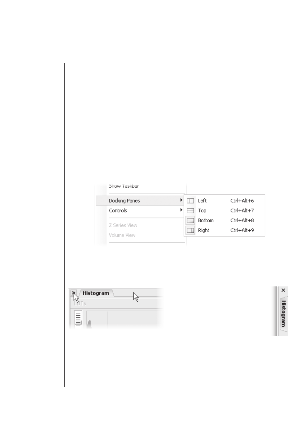
To display a docking pane
Docking panes are empty square spaces inside the application window, where you can place
(„dock“) the control windows. They can help to keep the screen „tidy“. There is one docking
pane available on each side (Top, Right, Bottom, Left).
- Go to the View>Docking Panes submenu and select the pane you would like to display.
- The docking pane appears, either empty or with some window(s) docked.
- Repeat this task to display more panes.
Hiding
docking pane
The same submenu can be also displayed by right-clicking into the empty application scre-
en.
To hide a docking pane
Either click the arrows in the top left
corner, or double click the empty pane
(not the docked control window). The
pane minimizes to a stripe by the edge
of the application. It can be recalled to
its original size by double clicking it.
Page 19
Page 22
Layout Manager
Shrink/Expand
docking panes
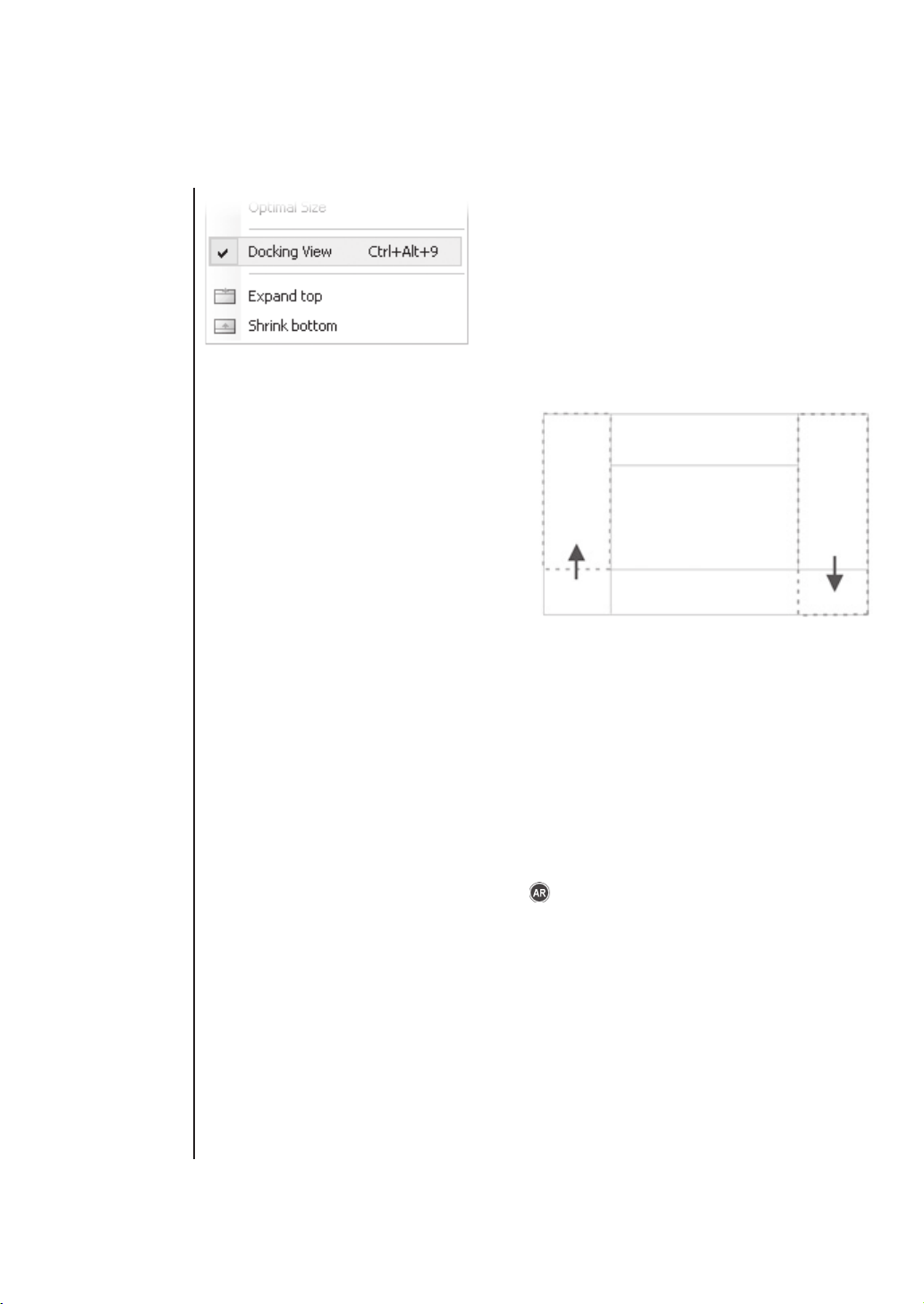
If you would like to close the pane completely, minimize it and press the cross button, or you can right click
the pane and unselect the Docking View option.
To shrink/expand docking panes
Having more docking panes opened, a
situation where there is not enough room for
the control windows can occur. In that case,
the Shrink and Expand commands shall be
used.
- Right click the pane you would like to
shrink/expand.
- A context menu appears.
- Select the Expand/Shrink command.
Control
windows
The commands Shrink/Expand Top, Right, Bottom, Left are available. When one of the panes
shrinks, the neighbouring pane expands to the emptied corner and vice-versa.
Control windows
The following control windows can be displayed within the application screen. They can be
fl oating, or docked inside the horizontal or vertical docking panes:
- 3D Measurement* (horizontal, req. EDF)
- Auto Capture Folder (horizontal)
- Camera Settings* (vertical)
- Filters and Shutters* (vertical)
- Histogram (vertical)
- Intensity Profi le (horizontal)
- LUTs (vertical)
- Lamp* (vertical)
- Measurement (horizontal)
- Microscope Control Pad* (vertical)
- Nosepiece* (vertical)
* - this control window is optional. A proper software licence or a correct device connected is
required in order to display it.
- Object Count (horizontal)
- Opened Views (horizontal, vertical)
- Preview (vertical)
- ROI Statistics (vertical)
- RT Deconvolution* (vertical)
- Time Measurement* (horizontal)
- View Synchronizer (vertical)
- Virtual Joystick* (vertical)
- Volume Measurement (horizontal,
vertical)
- Z Profi le* (horizontal, vertical)
Page 20
Page 23
Layout Manager
Displaying
control window
Closing control
window
Caption styles
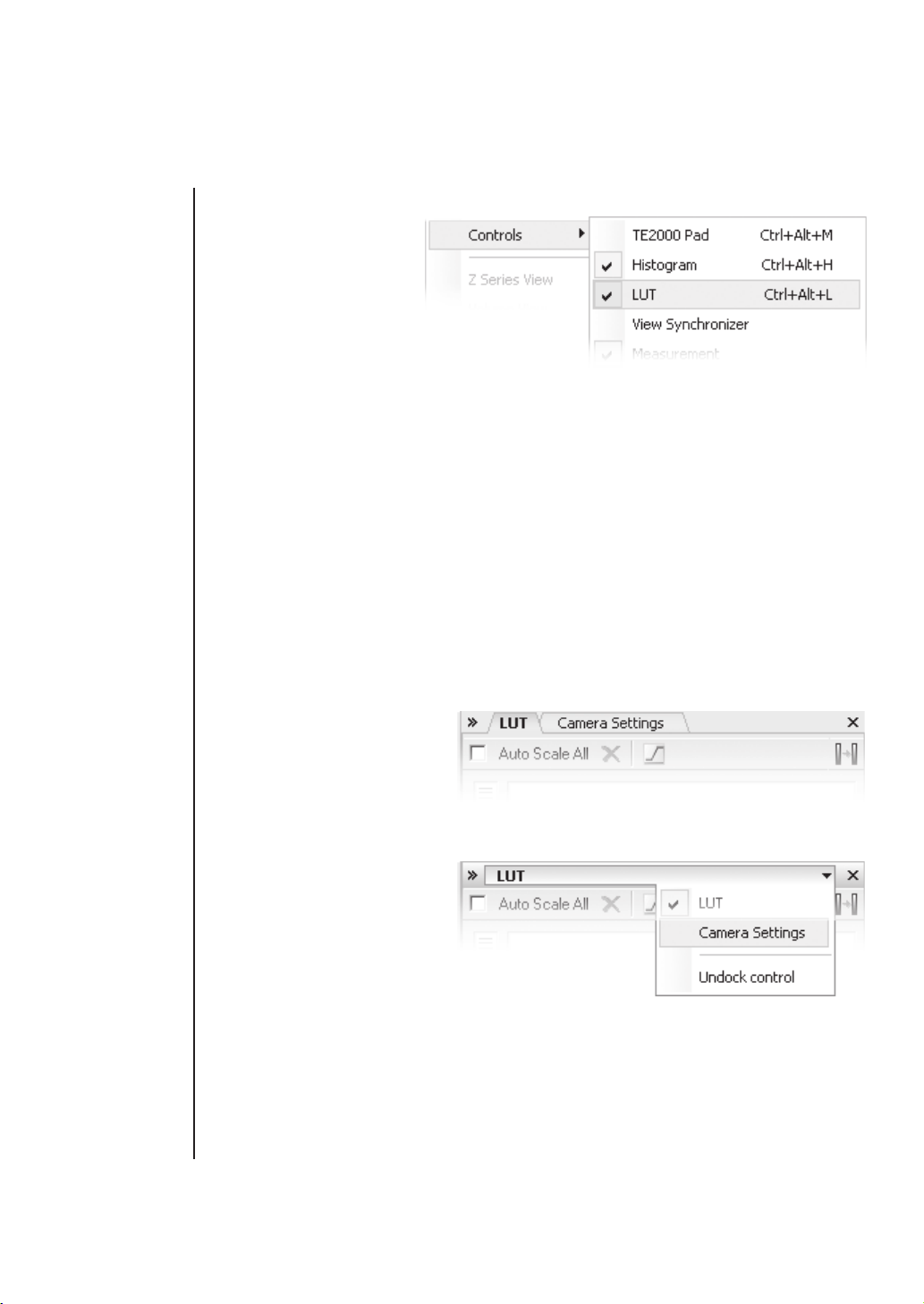
To display a control window
- Go to the View>Controls
submenu and select the
desired control window.
- The control window
appears fl oating on the
screen.
- To dock (and undock) it,
double click its caption.
It is also possible to display a control window docked. Right click inside a docking pane
and select the one of your choice. If the window is already opened somewhere (e.g. in the
opposite pane or fl oating), it closes and moves to the new destination.
To close a control window
- Click the „cross“ button on the right side of the active window caption.
- If the window is docked, you can also right click its caption and uncheck the appropriate
window.
- The control window closes.
Tab or caption style?
More control windows can be docked in the same place while only the front one is being
visible. There are two styles of displaying these windows, Tab and Caption.
Tab Style
- Besides the current control
window, the other window
tabs are visible.
- Switching the windows is a
one click operation.
Caption Style
- All docked windows except
the current one are hidden.
- The switching and undocking
of windows is done via the
menu that appears when you
click the arrow button.
Page 21
Page 24
Layout Manager
Managing
layouts
Creating new
layout
To manage layouts via the layout manager
The application can operate in two modes: supporting layouts or not.
To switch the layouts mode ON/OFF, reach the General Options tab
by double clicking the NIS-Elements caption. In the Appereance section, there is a check box
that enables/disables the mode.
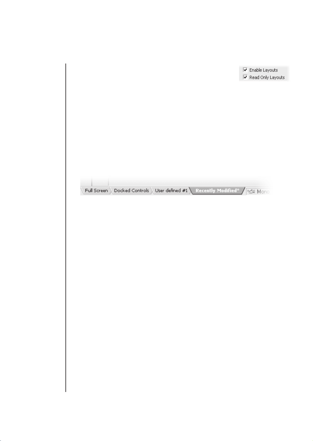
When you start the application with the Layouts mode ON, blue tabs representing active
layouts appear in the bottom left corner. The Full Screen and Docked Controls layouts are
placed by default. Other layouts can be added and managed via the Layout Manager.
If the „Read Only Layouts“ box is checked, no layout changes are saved during work or on
exit.
To create a new layout
- Modify the current layout to suit your concept of work.
- The asterisk appears next to the layout name (to indicate it has been modifi ed).
- Right click the layout tab and select the Save Current Layout As command.
- Write the new layout name and confi rm it by OK.
- A new tab appears and the layout is saved to the list of layouts.
If you do not need to create a new layout but would like to save the changes made, just right
click the current tab (asterisk-signed) and select the Save command from the menu.
Discarding
changes
Page 22
To reload previous layout settings
Unwanted changes of a layout may be made. Mostly, it can be fi xed by the Reload comma-
nd.
- Right click the asterisk-signed (recently modifi ed but not saved) tab and choose the
Reload command.
- The application restores the last saved state of the layout.
Page 25
Layout Manager
Using layout
manager
Layout manager
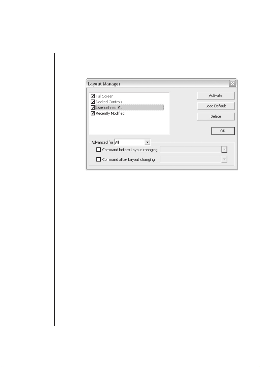
Right click any layout tab and select the Layout Manager command. The Layout Manager
appears.
- The check boxes on the left indicates the layout visibility (displayed/hidden)
- The Activate button makes the selected layout active (current)
- The Load Default button has the same functionality as the Reload command described
above. Except when applied to the Full Screen and the Docked Controls layouts where it
loads the original settings - so they look just the same as after the program installation.
- The Delete button deletes the selected layout. The fi rst two layouts cannot be deleted.
- Advanced settings enable to run a command or a macro right before and after a layout
change. It can be assigned to one or to all the layouts.
- The OK button stores all changes and closes the Layout Manager.
Page 23
Page 26

Layout Manager
Page 24
Page 27
Organizer
Organizer
Organizer
structure
Files view
Apart from the main application mode used for capturing and
image analysis, NIS-Elements provides a special Organizer
mode.
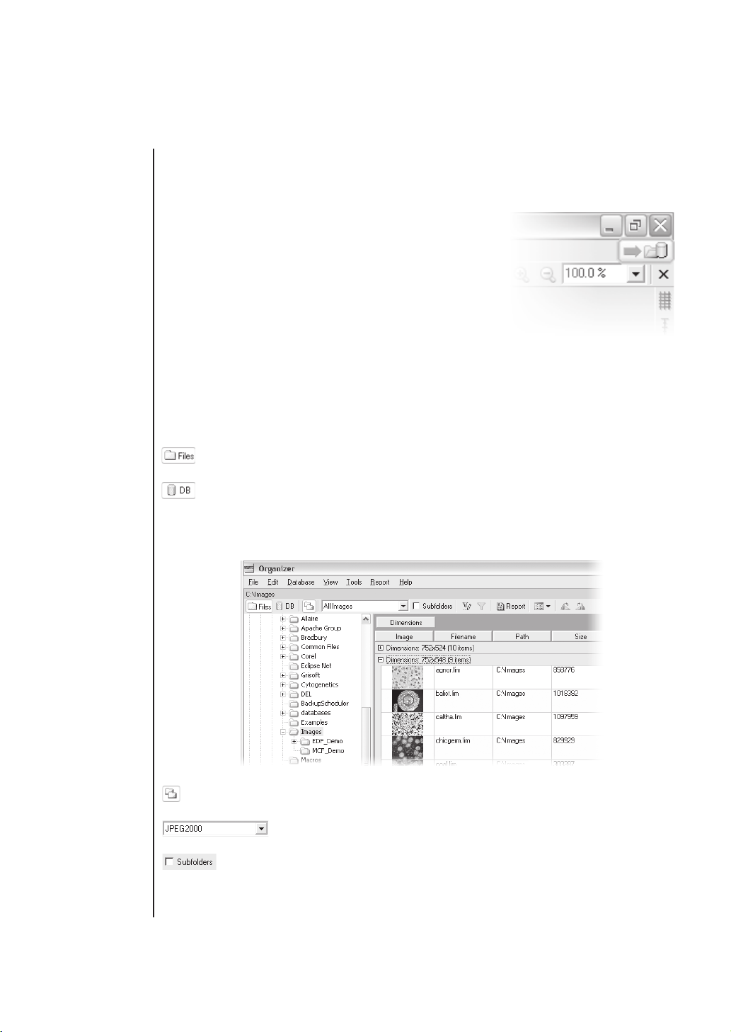
Organizer was designed to ease the work with image fi les
and databases. Clicking the Organizer button located in the
upper right corner of the NIS-Elements application window
or pressing F10 activates Organizer.
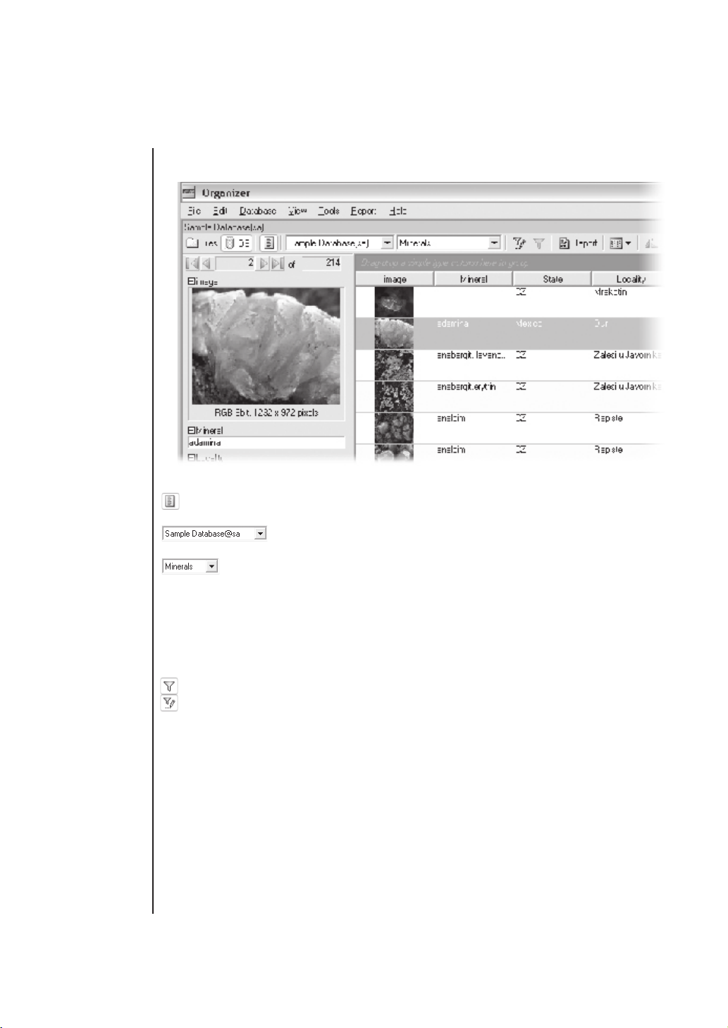
The screen is primarily divided into two identical panes. Each pane can be switched into two
modes: the Files mode and the Database mode. To switch from one pane to the other one
use „Next Pane“ command from the View menu. To copy fi les from one pane to the other one
simply drag selected images to the other pane.
- This button switches the pane to show a directory tree and images from the selected
folder (and its subfolders, when selected - see below). It is called the Files view .
- This button switches the pane to show the database structure and lists images
from the currently selected database table. This is called the Database view .
Features available in the Files view
- This button toggles the display of the directory tree. You can switch it off to get
additional space to display images.
- In this combo box it is possible to set the fi le type to be displayed.
You can select only a particular extension or show all fi les.
- If this check-box is selected all images from the included subfolders are
shown.
Page 25
Page 28
Organizer
Database view
Features available in the Database view
- This button toggles display of the database navigation and detailed information about
the selected image. You can switch it off to get additional space to display images.
- This combo-box displays the active connection point or enables to
select another defi ned connection point.
- This combo-box selects the database table and also indicates the current
table.
Filtering images
Page 26
Image fi lter
Both views (File and Database) have an option to use fi lters . It enables you to display only
such images, that match the criteria given.
- This button activates the fi lter.
- Pressing this button invokes the fi lter setup dialog box.
Page 29
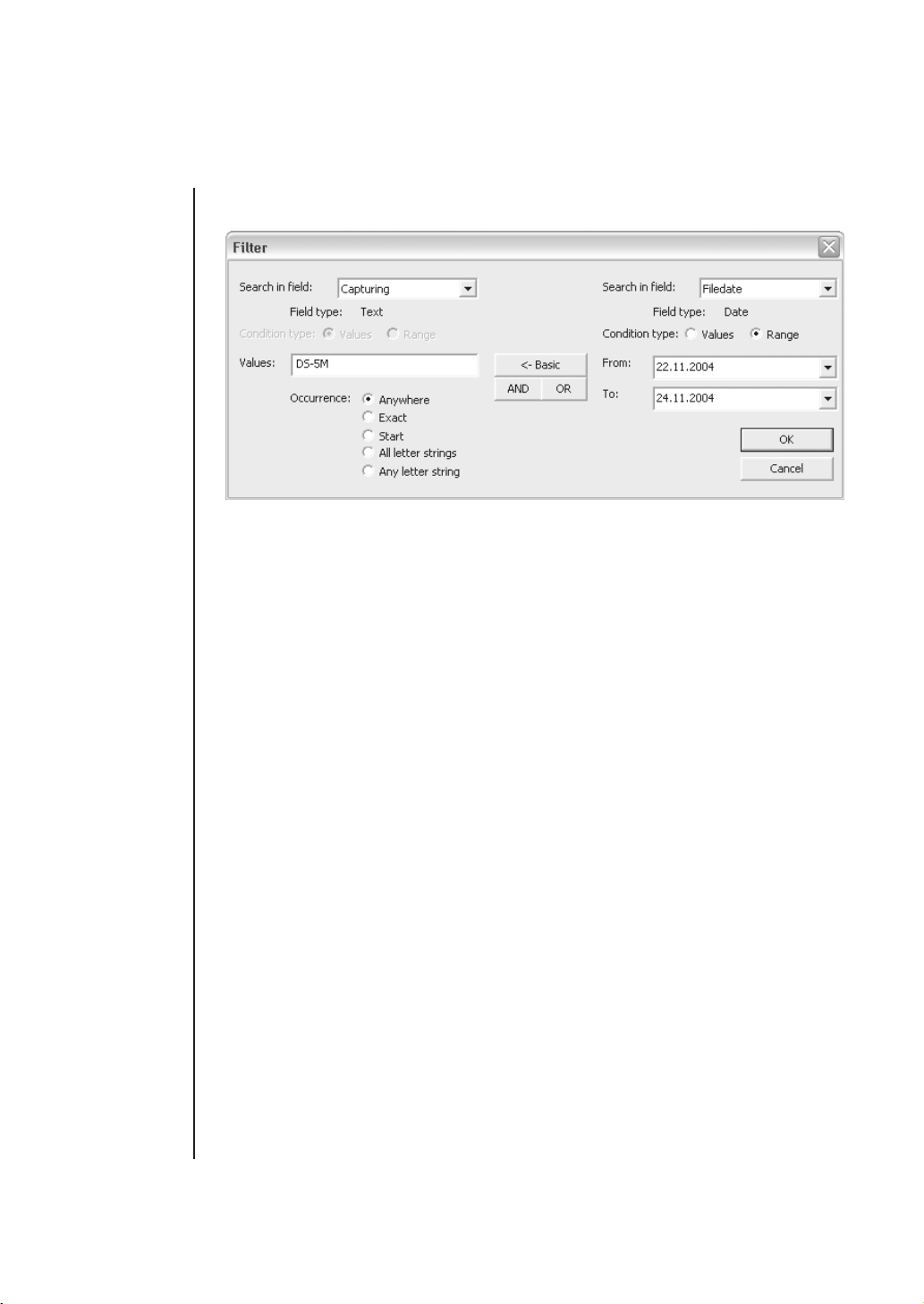
The fi lter can be used in two modes:
Organizer
Basic fi ltering
Advanced
fi ltering
Basic mode
This mode enables you to view fi les that match one defi ned condition.
Advanced mode
This mode enables you to defi ne two conditions with a relationship defi ned between them.
Either select OR to display fi les with the properties matching at least one given condition, or
select AND to display fi les the properties of which match both conditions at once.
First, select the fi eld, where NIS-Elements should search for a given expression. When using
a fi lter in the Files view, there are fi elds from fi le properties listed. In the Database view, the
listbox shows the names of fi elds from the currently selected database table.
If a selected fi eld is of a numerical type (e.g. Size, Calibration, File date etc.) you can specify,
whether you want to fi nd the exact value or a value in a given range (both displayed in the
picture above). This is selected by the Condition type radio button.
- Anywhere - If a given sequence of characters is found anywhere in the sequence of
characters in the fi eld, the system will evaluate it as a match. E.g. you have entered set
to the values edit box. The fi lter will select records with fi eld values: set , re set , set tings,
pre set ed...
- Exact - If the given sequence of characters exactly equals to the content of the fi eld, it
is evaluated as a match. E.g. if set is entered, fi elds containing the set value will only
match.
- Start - If the entered string is found at the beginning of a fi eld, it is displayed by fi lter. E.g
if set is entered, fi elds containing set , set ing set up are selected.
- All letter strings - It is possible to search for more expressions. These should be entered
separated by commas. If you want to enter an expression with a space, insert it into
Page 27
Page 30
Organizer
quotes. If this option is selected, only records in whose fi elds all of those expressions
(anywhere) appear are selected.
- Any letter string - This option is for entering multiple expressions as above, but this time
every fi eld with an occurrence of at least one from the given expressions is matched.
Operations with
images
Displaying
thumbnails
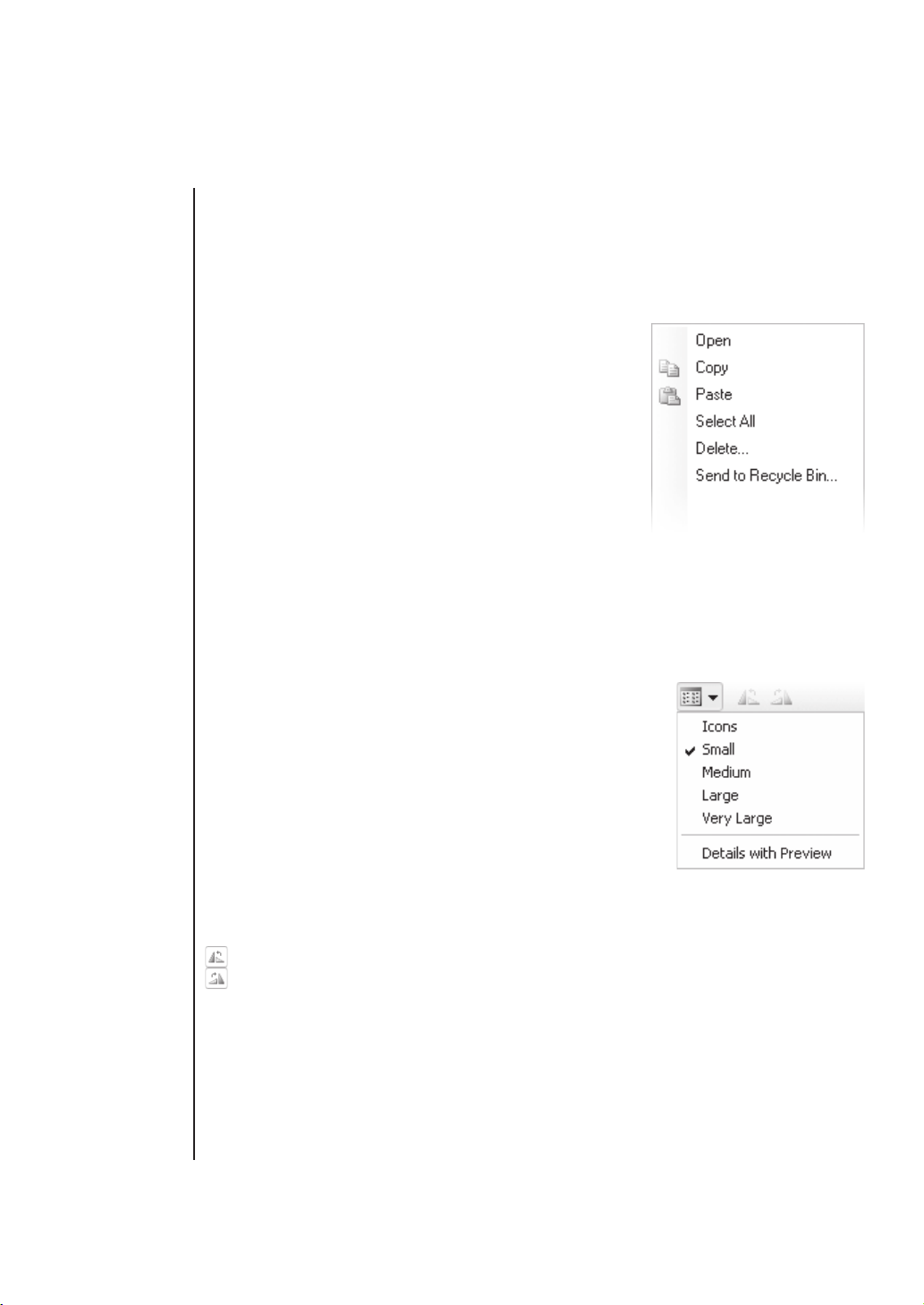
Operations with images
To open an image from the Files view, double click it. NIS-
Elements will display it in the main mode. To select multiple
images, either click on the fi rst and the last image holding
the Shift key (continuous group selection) or click individual
image names with the Ctrl key down to select more fi les that
do not appear together.
You can copy one or more selected images from one folder
to another only by dragging and dropping. This can be used
to ease inserting of images to the database too. Simply drag
the image from a folder and drop it onto the pane, where the
database table is opened. To delete selected images press
the Delete key.
All those operations and some other can be invoked also from the context menu, which
appears each time you right click on the image thumbnail:
Thumbnail displaying options
You can adjust the way images are shown in the panes. The
menu can be invoked in the main bar, where you can select the
size of displayed image thumbnails. Selecting the Details with
preview will display only one image per row with additional information about the image (image properties, if the images are in
folder or database fi elds, when viewing database records.)
Page 28
There is a possibility to rotate images which have wrong orientation. It doesn‘t affect just the display, but changes the underlying
image data too.
- Rotates image (or more selected images) left.
- Rotates image (or more selected images) right.
Page 31

Organizer
Images
sorting
Images
grouping
Adjusting
organizer
layout
Sorting of images
To adjust the order of displayed images, right
click anywhere in the pane. A context menu
will appear. Move to the Sort by command -
the submenu with several possible selectable
criteria will appear. If the sorting is already
active, the icon is displayed on the left side of
the selected sorting criteria (images are sorted
by their fi lenames).
Grouping of images
To better arrange the view of images one can use the grouping of images. Drag the column
name bar to the grouping bar (right above the column name bars). All fi les with matching
fi eld values of that column will be grouped together. This can be undone by dragging the
column caption back. See the example Files View picture above (the Dimensions column
is grouped).
Adjusting the look of Organizer
The pane size is adjustable. To resize it move the mouse cursor to the dividing in the middle.
The cursor becomes an arrow with two tips. Press the mouse button and move it to the new
position.
- Resizes the panes to achieve the same size of both of them.
- Resizes the pane to its maximal/minimal size (one pane is then displayed on the
whole screen).
Page 29
Page 32

Organizer
Page 30
Page 33

Setting the Hardware Up
Page 34

Page 35

Cameras
Cameras
This chapter is dedicated particularly to users running the active version of NIS-Elements equiped with a camera. Let‘s assume the camera works properly, is connected to the system
with proper system drivers installed and running (if required by camera).
Selecting driver
Selecting
camera
Selecting the driver
You will be asked to select the camera driver everytime you launch NIS-Elements. You can
change the driver later, using the Select Driver command from the Acquire menu. Choose
the driver that matches your camera:
Selecting the camera
Color cameras can be used in a monochromatic mode. The actual camera type (color/mono)
can be selected in the Acquire menu by choosing the Select Camera command. Confi rm the
choice with OK .
Camera setup
Live camera
signal
Setting up the camera
Exposure time, camera resolution, and other camera-specifi c features are adjustable
from the Camera Settings window. To invoke it, press the Camera Settings button
located on the left tool bar, or use the identical command from the Acquire menu. A
dialog window appears.
Live signal from camera
This button opens a new document window with the Live-Fast image from camera.
New buttons for controlling the camera appear in the document window to control the
camera.
Page 33
Page 36

Cameras
Live camera
formats
Capturing
images
Live formats
A format is a set of attributes of a video signal e.g.: resolution, bit depth, frame rate etc. Live
signal is a stream of image data, coming to your computer from the camera in real time. NISElements provides two different modes: Fast and Quality , each serving a different purpose.
The format of both modes can be set in the Camera Settings dialog box.
This tool bar button runs the Fast live mode. It is optimized to give as many frames
per second as possible in low resolution. This mode increases gain and uses short
exposure times.
This tool bar button runs the Quality live mode. It produces pictures in high resolution,
but the frame-rate is low. This mode sets the gain as low as possible and extends the
exposure time. This mode is applied every time the Capture button is pressed:
Capturing Images
Although it is possible to perform some procedures directly on the live image, other image
operations require captured or frozen images. If you try to perform such operation when the
live image is active, NIS-Elements automatically freezes the image. Let‘s see the difference
between Capture and Freeze functionality:
This is a Capture button. When pressed, the camera exposure runs till the end, and
the next frame is captured and displayed on the screen (the fi rst frame with the com-
plete exposure after you have pressed the Capture button).
The Freeze button interrupts the camera exposure, and displays the very last com-
plete frame.
Page 34
If you are using the fast mode and press Capture , NIS-Elements will automatically switch
to the quality mode to capture the image. When the image is captured, it is opened on the
screen as a new document.
Page 37

Hardware Confi guration
Confi guring Attached Hardware
Introduction
New optical
confi guration
Optical confi gu-
rations wizard
Typically, laboratory computer image analysis systems consist of a computer, a camera, and
a microscope equipped with all necessary accessories (objectives, fi lters, shutters, light,
various changers, etc). Most of the mentioned microscopic hardware is often motorized
and therefore can be controlled by NIS-Elements. Thanks to the NIS-Elements concept, it
is possible to integrate single settings of all these devices into one compact set called an
Optical Confi guration .
Creating New Optical Confi guration
Please check that all your devices (microscopes, cameras, etc.) that you want to associate
the new optical confi guration with are properly attached to the system and working. Insert a
calibration slide with reference objects of known sizes.
Start the Optical Confi guration Wizard
Choose the New Optical Confi guration command from the Calibration menu. The Optical
Confi guration Wizard starts. If a camera is connected, it is automatically set to Live mode.
- First type the name of the optical confi guration. We recommend to use short descriptive
names, e.g. name of the used objective.
- Then select the association to objective, camera or microscope. In case your typical
slides differ in brightness from the calibration slide, insert a specimen instead of the
calibration slide for this procedure.
- Use the Camera Setup button to adjust the camera image input. You can start the
illumination correction process by pressing the Capture Correction Image button.
- Adjust the Microscope setting by pressing the Microscope Pad button.
Press the Next button (when the Objective was selected) or Finish to continue...
Page 35
Page 38

Hardware Confi guration
Selecting
objective
Objective
calibration
Selecting Objective
Now, please select one of the following alternatives:
- Select one of already defi ned objectives from combo box or pick it from the pop-up menu
which appears after pressing the Insert button.
- Create a new objective by fi lling its name in.
Press the Next button to continue...
Objective Calibration
All digitized images consist of a number of small rectangular elements called pixels. A calibration assigns real size to one pixel, so correct measurements can be performed. Each
calibration depends on the associated magnifi cation, therefore it is necessary to create a
calibration for each objective. It is possible to assign names to objective calibrations and to
store them.
Page 36
Select one of the following alternatives:
Page 39

Hardware Confi guration
- The Manual calibration lets you draw a line into a picture and defi ne its real length (see
below). The „On Captured“ check box allows to decide whether a live or captured image
is used for a calibration.
- Having a motorized microscope, there are the Auto and 4 points alternatives available.
- Skip the calibration, if the selected objective (selected in the previous step) has been
already calibrated.
Press the Next button to continue...
Calibration
- manual
Manual Calibration
This step is dedicated to the manual calibration.
- The distance is defi ned by placing lines (Horizontal, Vertical, Parallel) in the image. First,
choose the lines orientation, then click into the image to place the fi rst line. Place the
second line in the intended location by another click. You can modify the line position
while holding the mouse button, not later.
- When Parallel lines are selected, fi rst defi ne the beginning of the fi rst line. The next click
defi nes its orientation and length. When satisfi ed, end the fi rst line creation by right-click.
The second line can be placed by another click into the image, this time to adjust the
distance from the fi rst line only. The process is completed again by right-click.
The following dialog box appears...
- Now enter the real distance between the two drawn lines and select correct units.
Press the OK button to continue...
Page 37
Page 40

Hardware Confi guration
Calibration
- automatic
Completion
Automatic Calibration (the Auto method)
This method is fully automatic. NIS-Elements moves the motorized stage, acquires two images, and calculates the calibration from the shift of the images.
Automatic Calibration (4 points method)
The system draws four points on the screen (subsequently) and asks user to move some
signifi cant part of the specimen by joystick to match the points. After all four steps are com-
pleted, the calibration is calculated from the moves of the stage.
Optical Confi guration Completion
Page 38
The last status window informs you about the parameters of the optical confi guration. Click
Finish to complete the process.
- You can create more calibrations by repeating the above procedures.
- The calibrations are stored to registry immediately and can be exported to a xml fi le
(Calibration > Optical Confi gurations > Backup).
- The selected calibration is maintained. It is applied during any image input from the
camera.
- The selected calibration remains unchanged even if a stored image together with its
(different) calibration would be loaded. After the camera input has been renewed the
formerly chosen calibration is restored.
- It is possible to adjust the created calibration. Select the Calibration menu > Optical
Confi gurations command.
Page 41

Hardware Confi guration
Selecting
optical
confi guration
Selecting Optical Confi guration
The active objective is displayed on the Status bar:
Buttons representing optical confi gurations are placed on the main toolbar. This feature is
set as default but it is possible to decide independently for every single Optical confi guration
whether to show its button or not. Pressing these buttons is the shortest way to switch among
the confi gurations.
The other way is to invoke the Optical
Confi gurations window (This can be
done by selecting the Calibration Menu
> Optical confi gurations or by right-
clicking the active objective name on the
status bar, and selecting this command from pop-up menu). The Optical
Confi guration dialog window appears...
Simply select the confi guration you
want to use, and click the Set as Active
button.
Recalibrating
captured
images
Recalibrating captured images
All images captured while a calibrated optical confi guration is selected are calibrated automa-
tically. If you need to change their calibration or you want to calibrate the image acquired via
scanner or transferred from digital camera, use the Recalibrate Document command from
the Calibration menu.
Recalibration is done the same way as the Manual Calibration described above.
Page 39
Page 42

Hardware Confi guration
Setting active
units
Setting Active Units
NIS-Elements supports following units: pixels, nanometers, micrometers, millimeters, centimeters, decimeters,
meters, inches, and mils. If the image is uncalibrated,
pixels are the only units available. In case of a calibrated
image, it is possible to select the desired units. All values
(e.g. measured length/area) are then displayed in the
corresponding units. There are two ways how to select
the desired units:
1) Right click on the document status bar section with
the information on image dimension and color bit depth.
A pop-up menu will appear. Select the units.
2) Or, click the Current unit button
located in the Optical confi gurations
dialog window and select the units.
Page 40
Page 43

Capturing Images
Page 44

Page 45

Images Capturing
Images Capturing
Having the whole hardware system set up and NIS-Elements installed, you can start capturing images. There are several ways of acquiring images, some of them specialized needing
specifi c hardware. The easiest way of all is to capture a single image:
Capturing single
images
Single Image Capture
- Turn the connected camera and other devices ON and start NIS-Elements. Select the
corresponding camera driver.
- When the application is started display the Camera Settings control window -
View>Controls>Camera Settings.
- Switch camera to live mode - Acquire>Live Fast - and adjust its parameters to get a clear
live image.
- Focus the objective on the scene you would like to capture an image of.
- Switch to the Live - Quality mode and adjust its parameters especially the Exposure time
and Format (this mode will be used every time an image is captured).
- Switch back to the Live - Fast mode. It is usual mode for smooth work because it uses
less hardware resources.
- Capture the image by pressing the capture button on the horizontal toolbar, by invoking
the Acquire>Capture command, or using the Ctrl+- shortcut.
- A new image is opened and named „Captured“ automatically.
Page 43
Page 46

Images Capturing
Page 44
Page 47

Timelapse Capturing
Time Lapse Acquisition
Detailed studying of long-lasting processes is enabled by the time lapse acquisition
mode of NIS-Elements. The possible experiment duration is almost limitless. Invoke the
Acquire>Capture Time Lapse command to set the experiment up:
Timelapse
options
Time Schedule
The Time schedule table enables you to defi ne consecutive time phases where duration,
interval between single images, and number of images of the phase can be adjusted for each
phase. The Interval, Duration, and Loops settings are bound together, so you just need to set
two of these parameters. The remaining parameter is calculated automatically.
Auto Focus
Automatic focusing can be used during experiment. You can select from the various
Autofocus methods that best meets your needs. The nearby combo box determines whether
the focusing shall be performed only at the begining of the experiment, at the begining of
each time-phase, or before each frame captured. The Defi ne button shows a dialog window
where you can defi ne parameters of the selected focusing method.
Special Options
The shutter can be closed between the acquisitions. Just check the Close Shutter... box.
Page 45
Page 48

Timelapse Capturing
The Advanced for combo box enables to run command (or macros) at the begining of each
loop. You can defi ne a common command (or macro) for all loops of the dimension or set a
command (or macro) individually for each loop.
You have an option to run a command* (or a macro) before and after Z-Series. It is possible to
enter the command directly, or press the rightmost button to show the context menu, where
you can select a command from list ( Command List ), or search for macro fi les on disk ( Run
Macro ).
* - The Live(); command can be used often. However, in some exceptional circumstances
the Live(); command may not work properly. In such case, please, use the LiveNoMsgLoop();
command instead.
Time
Measurement
Time Measurement
You can even Enable time measurement during acquisition . When no probes are defi -
ned, use the Defi ne Probes button. Please, see the Time Measurement chapter for further
details.
Page 46
Page 49

Multipoint Capturing
Multipoint acquisition
This feature is available when a mototized XY(Z) stage is present in the system and connected
properly. An arbitrary array of XY(Z) positions can be defi ned to be scanned during the mul-
tipoint capture experiment. The Z position can be included optionally. The defi ned array can
be saved (and loaded later) to an XML fi le by the Save button. Invoke the Acquire>Capture
Multipoint command.
Multipoint
options
To defi ne a multipoint array:
- Move the stage to the fi rst point (via a joystick or the „Move“ command).
- Press the Add New button. The new line containing current coordinates appears in the
list.
- Move to the next position and repeat the steps until you have all the intended points
defi ned.
To change a single Z coordinate:
- Click in the line you would like to change.
- Move the Z drive to the new position.
- Click the „<-“ button.
The XY coordinates of one point cannot be adjusted (unless you delete one and add a new
point).
Page 47
Page 50

Multipoint Capturing
Offset All
This button appears next to the currently selected point. It can shift the XY coordinates of all
points in the same way:
- Select one point of the list. (The stage moves to its coordinates automatically)
- Move the XY(Z) stage to a new position (defi ne the offset).
- Press the Offset All button.
- The coordinates of all points are rewrited (The same shift as you made is added/subtracted).
Special Options
Special Options
Please fi nd the description of all the other options in the Time Lapse Acquisition chapter.
Page 48
Page 51

Z Series Capturing
Z Series Acquisition
Capturing images from different focal planes of the specimen can be performed using the
Acquire>Capture Z Series>Capture Automatically command:
Z Series options
This dialog serves for setting the method of capturing in Z Series. Select between Absolute
positioning and Relative positioning
Absolute positioning
The two methods vary in the way the range is defi ned. The Absolute positions method
requires setting of two positions, by moving the stage and pressing the appropriate button.
The third position is counted automatically. For example if you defi ne Top and Bottom positi-
on, the middle one is set in the midle of these positions. Then if you move the stage and press
the Reposition button, all settings are recalculated so the middle value equals the current
stage position.
Relative positioning
Relative positions method can be used in Symetric (default) or Asymetric variation.
Symetric captures slices in range, that is same in both (up and down) direction from home
stage position. The value in Range editbox represent the whole range of capturing. When
selecting the Asymetric range checkbox, two editboxes, for defi ning individual range in each
Page 49
Page 52

Z Series Capturing
direction. The predefi ned values are halfs of the range defi ned in Symetric method.
Step Size
You can defi ne the step between images in Z axis manually, by entering the number of slices
or exact step size. It is possible to Use the automatically generated suggestion , that is
computed according to selected objective.
Page 50
Page 53

Multichannel Capturing
Fluorescence acquisition
Fluorescence (multichannel) pictures can be acquired using the Acquire>Capture
Multichannel Image>Capture Manually/Automatically commands. However, The
Multichannel setup should be adjusted fi rst (the Multichannel Setup command is located in
the same submenu):
Multichannel
options
Channels Setup
This table defi nes number and type of captured channels. First set a descriptive name, then
select the optical confi guration (from combo box) that is to be used for capturing the channel.
If any suitable confi guration does not exist, you can create a new one, by selecting the defi ne
new option (when clicking on the down arrow button next to the Optical Confi guration name).
Comp. color specifi es the color tone, in which this channel will be displayed.
Page 51
Page 54

Multichannel Capturing
Manual Filter Change
The Wait for user before changing to next channel option enables you to switch the wa-
velength fi lters manually during the multichannel experiment. Use this option if there is no
automatic fi lter changer available.
Autofocus
The Autofocus settings are applied within the automatic multichannel acquisition only. When
capturing multichannel images manually, the autofocus is not available.
Automatic
Capture
Manual
Capture
Automatic Capture
The Capture Automatically command runs the automatic multichannel acquisition procedure
according to the Multichannel Setup settings. When the procedure is fi nished, the resulting
multichannel document is opened.
The automatic capture can be performed even you do not have a motorized fi lter changer.
The Wait for user before changing to next channel option must be checked. Then a con-
fi rmation dialog box before each channel acquisition appears.
Manual Capture
The Capture Manually command opens a new document window with the
live image and the Capture button. After pressing the Capture button one
channel is captured. The number of channels depends on the Multichannel
Setup.
A single channel may be recaptured by the Live button during before the
experiment is fi nished. Select the channel and press the Live button that
appears instead of the Capture (at already captured channels).
After all channels are acquired, the Recapture button replaces the Capture
button. It enables you to capture the multichannel document again. All
previously obtained multichannel data will be lost. When a single channel is
selected, it can be recaptured separately.
Page 52
Page 55

Capturing to Ring Buffer
Capturing to Ring Buffer
Capturing to
RAM
Ring buffer size
The Capturing-to-RAM technique enables user to record sequences displaying very quick
actions, lasting tens of miliseconds. The quality and number of frames in a sequence depends
on hardware capabilities of the computer system.
Set the ring buffer size
The technique uses a ring buffer to store temporary data. The ring buffer is a part of virtual
memory that is being constantly (and repeatedly) fi lled with the live image data. Depending
on how fast the action to be captured is, you should set the ring buffer size in miliseconds.
- Click on the Settings command next to the RAM capture
buttons.
- Set the Time buffered before/after values. These
represent the time before and after you click the RAM Capture button. The whole time
interval will be included in the sequence.
- Confi rm it by OK.
Buffer ON/OFF
Turn the buffer ON
- Click on the leftmost button of the RAM capture tool bar to enable recording of Live image
to RAM.
- The ring buffer functionality is activated.
When the Camera is switched to Live mode, the left-side ring icon begins to indicate the buffer
activity. If the RAM Capture button is pressed then, the captured sequence contains frames
from the whole time interval before and after the button press. If you press the button while
in the Frozen mode or without the time buffer ON, only the Time buffered after sequence is
grabbed.
Page 53
Page 56

Capturing to Ring Buffer
Capturing a
sequence
Capture a sequence
- Press the RAM Capture button.
- A new document window containing the captured seqence opens.
Page 54
Page 57

Documents, Archiving
Page 58

Page 59

Document Structure
NIS-Elements Document Structure
Image Layers Image Layers
Each captured image can consist of the following image layers, serving different purposes:
Annotation layer - In this layer, graphi-
cal objects and texts can be stored in a
vector format. The results of interactive
and automatic object measurements,
arbitrary text notes and other annotations are stored there.
Binary layer - Pixels in this layer can
be found in two states only (i.e. Black/
White). A binary image is usually result
of thresholding. It is used mainly for
performing automatic measurements
of the thresholded objects.
Document types
Color layer - Contains image data.
When you open an image from disk,
it is loaded to this layer. It can handle
images with the depth of up to 16 bits
per color component. The dimensions
of this layer determine the view of the
other layers.
When saving an image, only the JPEG2000 and ND2 fi le formats can handle all image layers
and are capable of saving them. The other image formats will save the content of the color
layer only.
Document types in NIS-Elements
RGB documents
Images acquired by a color camera typically consist of three components that represent red,
green and blue channel intensities. Pixel values for each component range from 0 to 65535
(in 16 bit depth). You can display a single color channel using the tabs located in the bottomleft corner of a document window.
Page 57
Page 60

Document Structure
Multi-channel documents
These documents arise usually from fl uorescence microscopy. Instead of 3 color components
(R, G, B), multichannel images can be composed from many user-defi neable color planes.
When a multichannel image is opened, the channels panes (bottom-left corner) are not the
standard ones (marked with Red, Green, Blue), but are named differetly according to the
different colors. The maximum number of channels are 32.
If there is a document that contains more than 8 components, the tabs are replaced by the
Lambda dimension, similarly as other dimensions of ND2 documents are displayed.
ND2 (N dimensions) documents
The ND2 document is in fact a set of images. There are four types of ND documents depending
on the method of acquisition: T for timelapse acquisitions, XY for multipoint acquisition, Z for
Z-series (slices) acquisition and Lambda for acquisition of a defi ned wavelength (fl uorescen-
ce imaging). All these methods can be combined together. In the most advanced case, you
can have image data from defi ned time periods captured in different positions of an XY stage,
each image can be displayed in defi ned numbers of its Z slices and each slice can consist of
number of planes, where each plane can be acquired using different light wavelength. All the
images captured by these methods can be stored to a single fi le.
Document
window
Document window
Since NIS-Elements supports multiple windows, all controls affecting the view of the image,
its layers, and components are located in every image window. Therefore it is possible to
control each opened image individually.
Page 58
Page 61

Document Structure
Document
control buttons
LUTs
- Enable LUTs button applies LUTs to the image.
- Keep Auto Scale LUTs button applies the AutoScale command to the image conti-
nuously.
- Auto Scale button performs automatic setting of LUTs .
- Reset LUTs button discards the LUTs settings.
Zoom controls
- Fit to screen toolbar button. Adjusts zoom to view the whole image in its maximum
magnifi cation. It corresponds to the Fit to screen command .
- Best Fit toolbar button. It adjusts zoom to view the image as large as possible in
NIS-Elements image window. Corresponds to the Best Fit command .
- 1:1 Zoom toolbar button. It adjust the zoom to view the image in its original magnifi cati-
on. It corresponds to the 1:1 Zoom command .
- Increases magnifi cation. It corresponds to the Increase command .
- Decreases magnifi cation. It corresponds to the Decrease command .
General controls
- Show Probe button activates the probe. The probe affects histograms, auto exposure
and auto white functions.
- Show Background Probe toolbar button activates the background probe. Some
commands (Subtract Background) uses the BG probe data as reference.
- Show Grid button displays the grid for rough measurements.
- Show Scale button displays the scale.
- Show Frame button displays and applies the measurement frame.
- Show Measurement ROI button displays the Measurement ROI.
- Show Profi le toolbar button displays the intensity Profi le window. This tool alows
you to specify direction in the image (using arrow) and the graph displays intensity of
pixels, that this arrow passes trough.
Document
status bar
Right click the icons to invoke a context menu where properties of each tool can be modi-
fi ed.
Status bar
The status bar at the bottom shows the following information (from left to right): pixel coordinates of the mouse cursor with channel intensities, color mode, bit depth, and picture size
in pixels.
Page 59
Page 62

Document Structure
Annotation
layer
Working with the Annotation layer
This button toggles viewing of annotations. Right-clicking the button displays the
following context menu:
- Clear Annotations will remove all objects
from this layer.
- Remove Automatic Measurement
objects will remove only objects created
by automatical measurement. Other
objects remain untouched.
- Select Interactive Measurement
objects will select all measurement
objects created by user.
- Select Annotation Objects will select
all objects that are not the measurement
ones.
- Select All Objects and Deselect will select / unselect all objects stored in this layer.
This button toggles viewing of the measurement objects of the interactive and automatic measurements.
Working with
binary images
Working with Binary layer
This button switches to a view of the binary image. It can be edited by hand using
Binary editor command from the Binary menu, or by pressing the Tab key.
The Binary layer can be displayed together with the color layer using the Overlay
mode . The appearance of the binary layer can be modifi ed by right clicking the
Overlay Mode icon.
This button switches to a view of the color image. When working with RGB image, this
layer consist of 3 separate components (Red, Green, Blue). When working with multichannel images, there can be a lot more channels. You can view all these channels
mixed together or you can work with (process) only one single channel. To choose it,
click on the tab located in the bottom left corner of the document window.
The selected component is marked by color underlining and the pane moves optically to
front. ( Red is selected in the image.) To edit the name or color of component, click on the
tab by right mouse button and choose the command from pop-up menu. Custom number of
components can be selected while holding the Ctrl key down.
Page 60
Page 63

Working with Documents
Working with Documents
When working with documents it is possible to work with multiple images opened at the same
time. If an image has been opened and another one is opened next, the original doesn‘t
close and remains loaded in memory. The Multi-Document Window Environment ensures
that every document is opened to a single window that contains the most used controls
affecting the image appereance (Layers, LUTs, Zoom etc.).
Opening Saved Files
NIS-Elements offers several ways to open an image fi le:
Open dialog box
Organizer
Recent fi les list
Using the Open dialog-box
To invoke the Open dialog box, you have the following options:
- Select File menu - Open command...
- Press Ctrl + F12 keys simultaneously...
- Press the Open button located on the main NIS-Elements toolbar (left side of the
application window)...
Using the Organizer
An image can be opened by double clicking its fi lename within the
Organizer layout. More information can be found in the Organizer
chapter.
Using the Recent fi les list
You can quickly access the last opened images using the Recent fi les submenu from the
File menu. The number of listed fi les can be changed by user in the General Options window
(double click on NIS-Elements caption to display it).
Open next
command
Using the Open next/previous/fi rst/last command
These commands enable you to continuously open the next/previous images from a defi ned
directory or database table. This is useful when editing multiple fi les placed in one directory.
The commands are located in the Open/Save Next submenu of the File menu. You can
defi ne sorting, fi ltering and other features in the Open Next settings dialog box.
Page 61
Page 64

Working with Documents
Windows
explorer
Straight from Windows explorer
During installation, NIS-Elements creates fi le associations to fi les that are considered a native
format for storing images (JPEG2000, ND2). The JPEG2000 (JP2) and ND2 image fi les can
be then opened in NIS-Elements just by double clicking their names in Windows explorer.
Switching between loaded documents
The commands for managing the opened
images are grouped in the Window menu.
The presently opened fi les are listed in its
bottom part. The currently displayed image
is indicated by a check mark on the left side.
To change the current image, simply click the
window with the desired document. If it isn‘t
possible because of many opened windows
overlapping the one you would like to view,
select it from the list or use the Next or the
Previous command (represented by Ctrl +
Tab and Ctrl + Shift + Tab shortcuts). Another
possibility is to arrange document windows
automatically using the Tile horizontally or
Tile vertically commands. This will change
the size and position of all opened documents
and these will be aligned like tiles in selected
direction.
Page 62
Amount of opened images at one time
In NIS-Elements, it is possible to set the maximum number of images opened at one time.
This is done in the General Options dialog box that is displayed after double clicking the
NIS-Elements caption.
The amount is set in the List of opened documents contains n documents edit box. If you
set this parameter to 1, NIS-Elements will behave like a single document interface.
Page 65

Working with Documents
Closing documents
The currently displayed image can be quickly closed by pressing the close window
button, located in the upper right corner of the NIS-Elements document window . (The
image displayed below shows the close button of a maximized document.)
The image can be also closed by invoking the Close command from the Window menu or
by pressing the Ctrl+F4 shortcut. If you want to close all images use the Close all command
from the same menu, or the Ctrl+Shift+F4 key shortcut. If you try to close an image that
has been changed, NIS-Elements will display a confi rmation dialog box, offering to save
changes.
Supported
image formats
Image Formats
NIS-Elements supports the following number of standard fi le formats. In addition, NIS-Elements
uses its own image fi le formats (JP2, ND2) to fulfi ll specifi c application requirements.
JPEG2000 Format (JP2)
An advanced format with optional compression rates. Image calibration, text descriptions,
and other meta-data can be saved together with the image in this format.
ND2 Format (ND2)
This is the special format for storing sequences of images acquired during ND experiments.
It contains various information about the hardware settings and the experiment conditions
and settings.
Joint Photo Expert Group Format (JFF, JPG, JTF)
Standard JPEG fi les (JPEG File Interchange Format, Progressive JPEG, JPEG Tagged
Interchange Format) used in many image processing applications.
Tagged Image File Format (TIFF)
Developed by Aldus and Microsoft to promote the use of desktop scanners. Used for compatibility with other applications. This format includes information about author, sample, subject,
and calibration. Because TIFF fi les do not have a single way to store image data, there are
many versions of TIFF. The system supports the most common TIFF modalities.
CompuServe Graphic Interchange Format (GIF)
This is a fi le format commonly used on the Internet. It uses a lossless compression and stores
images in 8-bit color scheme. GIF supports single-color transparency and animation. GIF
does not support layers or alpha channels.
Portable Network Graphics Format (PNG)
This is a replacement for the GIF format. It is a full-featured (non-LZW) compressed format
intended for a widespread use without any legal restraints. NIS-Elements does not support
the interlaced version of this format.
Page 63
Page 66

Working with Documents
Windows Bitmap (BMP)
This is the standard Windows fi le format. This format does not include additional image
description information such as author, sample, subject or calibration.
LIM Format (LIM)
Developed for the needs of laboratory image analysis package. Nowadays, all its features
(and more) are provided by the JPEG 2000 format.
ICS/IDS image sequence
ICS/IDS sequences are generated by some microscopes and consist of two fi les: the ICS fi le
with information about the sequence; the IDS fi le containing the image data. The ICS fi le must
be stored in the same directory together with the IDS fi le.
Page 64
Page 67

Image Analysis
Page 68

Page 69

Histogram and LUTs
Histogram and Look Up Tables
Histogram
basics
Histogram
controls
Histogram Window
Histogram is a graphic representation of number of pixels (Y axis) in the image versus their
pixel values (X axis). The pixel values run from 0 displayed as black to 255 - 65535 (depending on the image bit depth) displayed as white. In case of grayscale images a vertical bar
is plotted for each pixel value showing the number of pixels in the image with that value.
Considering color images, such graph is displayed for every color component.
The picture above shows a standalone histogram window. When this window is docked, it
shows only the most signifi cant information to spare space.
Histogram controls
- This button switches the histogram view to a mode with three separate
graphs, one for each color component.
- This button switches the histogram view to a mode where all colors and
intensity curves are displayed in one graph(see the picture).
Normally, the histogram shows data of the original image. If the LUTs button is activated, the
histogram displays data as if LUTs were applied.
Page 67
Page 70

Histogram and LUTs
Look Up Tables
LUTs on RGB
LUTs
A look-up table represents a useful tool for color modifi cations. It takes a value, maps it to
a location in a table, and replaces the incoming value with the contents of the table entry.
There are 3 modes of LUTs, depending on the image you are processing. Different controls
will be available when applying LUTs to monochromatic, RGB, or multichannel image. When
LUTs are activated the LUTs button in the upper left corner of the document window is
highlighted.
LUTs on RGB images
Page 68
The main part of LUTs window is occupied by a histogram view. There are 3 separate curves
for each RGB component, and one gray fi lled curve for the whole image. You can adjust the
histogram view by moving the slider on the left part of the window.
The black and white triangular sliders defi ne threshold. All the pixels with values lower than
the black slider indicates (left of the slider) will be displayed as pure black. Everything to
the right of the white slider (all pixels with higher values) will be displayed as white. The
remaining color shades will be composed of the pixels with values between the two sliders
with defi neable gamma parameter. Gamma is adjustable by moving the gray slider.
- This button extends the sliders and displays the histogram as if LUTs was applied.
The range of pixel values currently displayed becomes indicated in the top right corner.
Page 71

Histogram and LUTs
Three color bars with sliders (displayed underneath the histogram) are representing RGB
components. The slider movement affects the brightness of each component.
Auto scale
LUTs
Auto scale
The auto scale mode automatically sets the white slider and gamma parameters to get
the best image view (what is „best“ is determined by a universal algorithm, that may
differ from your needs). If you select the Use Black Level parameter from the pop-up
menu, the black slider will be affected too.
It is possible to apply the Auto scale procedure only once by pressing the button, or to
run it permamently (on the live image) by clicking the Keep Auto Scale button. When
you turn the Keep Auto Scale off, the settings remain as if the Auto Scale button was
pressed once. If you want to discard all LUTs settings, press the red cross button,
located next to the Auto scale button.
Settings
Press the arrow next to the Auto Scale button, a pop-up menu will appear. Invoke the Settings
command.
Quantile (0-10%) - this value determines how many of all pixels of the picture are left outside
the sliders when LUT is applied.
White balance
Tolerance (0-10%) - if the threshold decreases within the set Tolerance, LUT remains unchan-
ged and is not re-counted. When the change exceeds the Tolerance, LUT is recounted. This
reduces number of LUT calculations when the camera produces picture noise.
AWB
AWB (Auto White Balance) mode adjusts the image to get the color neutral white. Similarly as
above, it can be used once, or permanently on the live image by clicking into the Keep Auto
White Balance checkbox left of the AWB button. When you uncheck the box, the settings
remains as if the AWB button was pressed once.
If you know which undertone your white has, you can select this color by the color picker that
appears after pressing the ... button on the right of the AWB button. And again, all changes
are discarded using the red cross button.
Page 69
Page 72

Histogram and LUTs
- The color overexposed button. When this button is activated, all pixels whose values
reach maximum will be highlighted.
- Press this button to apply the LUTs settings to the color image data. Until you press
this button, no changes are made to the image data.
LUTs on mono
images
LUTs on Monochromatic images
All things mentioned above are also valid for monochromatic images. When adjusting a
monochromatic image, you don‘t have AWB function available and the whole image is controled using only one bar with sliders. On the other hand, you can set more modes of displaying,
including colorizing the image using predefi ned color schemes.
Page 70
This pop-up menu is used for pickng the mode of mapping. You can
select from Contrast or Window modes. When Contrast is selected,
all pixels with values higher than the white slider will be set to white.
But when Window is active all pixels with value higher than the white
slider will be set back to black.
This button indicates the selected color table and displays
this pop-up menu. There you can select the color scheme, in
which you want to display your image. Try a few of them to
see which highlights most of the details you want to see.
Page 73

Histogram and LUTs
LUTs on
multichannel
images
LUTs on Multichannel images
In case of multichannel image the histogram shows different color curves - each color for
one component (channel). You can adjust any channel you want using the corresponding bar
placed at the bottom of the LUTs window.
- A single channel can be adjusted automatically using this Auto scale button.
Look-up tables are useful for equalizing images. For example, if the image is very dark (which
usually happens with quantitative cameras), you can restrict the view to display just the low
pixel intensities. Hidden details become more apparent.
Page 71
Page 74

Histogram and LUTs
Page 72
Page 75

Binary Editor
Binary Editor
Binary Layer
The binary layer, as a result of thresholding, can be modifi ed by hand using the binary layer
editor. It is a built-in application providing various drawing tools and morphology commands.
Go for the Binary Editor command in the Binary menu or press the Tab key. New controls
appear on main application toolbars:
Controls (horizontal tool bar)
- Reverses the changes made to the binary image. <U>
- Clears the binary image (fi lls the entire image with the „background“ color). <R>
- Loads the image previously saved by the Save button. <L>
- Temporarily saves the current binary image. It can be loaded anytime before the
binary editor is closed by the Load button. <S>
- Displays this help page.
- Stores the changes and quits the editor. <ESC> or <TAB>
The other buttons of the vertical tool bar are simplifi ed versions of mathematical morphology
functions. Please see the Mathematical Morphology Basics chapter for more details.
- Dilate
- Erode
- Close
- Open
- Separate Objects
- Clean
- Fill Holes
Drawing tools (vertical tool bar)
The binary image can be modifi ed using various drawing tools. Although the way of use of
some tools differs, there are some general principles:
- Make sure you are in the right drawing mode (drawing background/foreground)
- Any object that has not been completed yet can be canceled by pressing Esc .
- The polygon-like shapes are drawn by clicks of the left mouse button. The right button
fi nishes the shape.
- The auto-drawing tools (threshold, auto detect) have a changeable parameter. It can be
modifi ed by +/- keys or by mouse wheel.
- The scene can be magnifi ed by the UP/DOWN arrows when mouse wheel serves another
purposes.
- The right mouse button drags the image when magnifi ed.
- A line width can be set in the upper left corner.
- Hints are displayed below the horizontal tool bar.
Page 73
Page 76

Binary Editor
Auto white
balance tool
Drawing tools
- Switches between the foreground and the background editing mode. <Ctrl + SPACE>
- The Hand tool. Serves for moving the image when magnifi ed. <Ctrl+W>
- Bezier hollow tool. The object is defi ned by placing points on its perimeter. The lines
connecting those points can vary from straight lines to bezier curves. (Use +,- keys to
adjust them). To fi nish creation press the right mouse button. <Ctrl+F11>
- Bezier fi ll tool. It equals the Bezier hollow tool, but the resulting object is fi lled.
<Ctrl+F12>
- Draws a fi lled polygon. While holding the left mouse button down, you are in the
free hand mode. When you release it, each click defi nes a corner of the polygon. The
polygon is enclosed and fi lled by pressing the right mouse button. <F4>
- Draws a polygon. It equals the Filled polygon tool, but the resulting object is not fi lled.
<F3>
- Draws a fi lled circle. Click to determine the center and defi ne the perimeter holding
the left mouse button down. <F8>
- Draws a circle. Click to determine the center and defi ne the perimeter holding the left
mouse button down. <F7>
- Draws a fi lled rectangle. <F10>
- Draws a rectangle. <F9>
- Draws a fi lled moveable circle/ellipse. If you grab the ellipse near the center, you
can move it. If you grab it near the border, the nearest semi-axis is being modifi ed.
When holding down either the SHIFT or the CTRL key, both semi-axes change equally
(forming a circle). <F12>
- Draws an ellipse. <F12>
- Drawing by hand. <F1>
- Draws a straight line. <F2>
- Draws a polyline. <F5>
- The Auto Detect fi
image to place the probe, the detected area is drawn. You can adjust the thresholding
range by using the mouse wheel or by pressing the +, - keys. <Ctrl+B>
- Threshold tool. Click into the image to place the probe (or more of them) to defi ne the
initial color level for thresholding. Pres +,- keys or use the mouse wheel to change the
thresholding range. <J>
- Fill an enclosed shape. <F6>
- Area of interest. Entities outside the selected region will be cleared.
- Text tool. Displays dialog box for defi ning text parameters.
- Commands tool. Displays a pop up menu offering user some additional commands:
lled tool. Detect hollows using threshold techniques. Click to the
Page 74
Page 77

Binary Editor
Commands
Commands
- The Auto Detect hollow tool. Detect hollows using threshold techniques. Click to the
image to place the probe, the hollow is drawn. You can adjust the thresholding range
by using the mouse button or by pressing the +, - keys.
- Draws rectangularly crossed lines.
- Draws a rose. Click to the image to defi ne the center, than drag the mouse to set the
length of it‘s arms.
- Places a marker to the image. Simply click into image...
- Selects binary objects.
- The Connect tool. Draws a line(s) from the point you‘ve clicked on, to the nearest
object(s).
- Displays a grid. Visible only when using magnifi cation 400% and higher.
- Hides the binary image and displays the just the color image.
- Inverts the binary image. Foreground becomes background and vice versa.
The last two buttons perform simplifi ed versions of mathematical morphology functions.
Please see the Mathematical Morphology Basics chapter for more details.
- Smooth
- Contour
Tools are either applied in a „draw“ (foreground) or „erase“ (background) mode. Some tools
(like threshold or bezier) have editable parameters. Tips how to use the tools are displayed
in the vertical toolbar.
Page 75
Page 78

Binary Editor
Page 76
Page 79

Measurement
Measurement
Measurement is an advanced and complex image analysis technique. It starts with calibration of the NIS-Elements system which is followed by a quantitative evaluation of the image.
Image analysis is fi nalized with data examination and presentation.
Calibrating
system
Rough
measurement
Calibration
Calibration is of a crucial importance for the measurement. It assigns real sizes to objects,
so they can be compared to each other. A correct calibration has to be made before the
measurement begins. See the Optical confi gurations section explaining how to calibrate
the NIS-Elements system.
Rough Measurement
Quick and approximate measurements can be performed with the graticules. They
behave like adjustable fl oating rulers. The user can simply align it with the measured
object and read the distance (e.g. the diameter). To activate a graticule, press the Graticules
button placed in the upper-right corner of the document window ) The type of the graticule
ruler is indicated by a picture on this button. The types are: Rectangular , Circle , Cross ,
Vertical Ruler , and Horizontal Ruler .
To change the graticule type, click on the graticules button with
the right mouse button and select the appropriate item from
the context menu. The menu also contains two commands for
placing the graticules ruler into binary image layer and vice
versa. The command Move Graticules to Center aligns the
center of the ruler with the current center of screen. The last
command - Graticules properties - displays the following dialog
box:
Measurement
options
In this dialog box all parameters
(shape, color, line width, density of
lines) can be adjusted. The density
value - the closest distance between
two line intersections of the graticule
- can be set in pixels (in case of
uncalibrated image) or in selected
units. The density can be also
adjusted automatically according to
the current zoom factor.
Page 77
Page 80

Measurement
Interactive
measurement
Interactive measurement
The interactive measurement procedure means that the user measures directly on the screen
and gets precise outcome in selected units. The measurement is performed by drawing e.g.
two parallel lines, aligned with borders of the measured object. This is the way of defi ning
the boundaries of the object in the image. The real size of the object is then counted using
calibration constant.
The interactive measurement can be performed on both color and binary images. First,
select the feature you want to measure. You can choose from: Taxonomy , Counts , Length ,
Semiaxes , Area , Angle or Profi le . The selection is done by picking one of those commands
from the Measurement menu. For example, to measure the distance between two objects in
the image, select the Length command and the following dialog box appears:
Page 78
The buttons in the upper part of the window represent different measuring tools. Detailed info
about any of measuring tool can be found in the Command Reference section of the help.
The following example illustrates how to measure the size of a crystal on its binary image:
Select the interactive tool Horizontal parallel lines . Place
the fi rst line to its position by clicking into the image. Hold
the left mouse button during positioning, after you release
it, the line is positioned. Repeat it for the second line.
When fi nished, an arrow is drawn between those lines,
joined by the value of the measurement. A record with the
measurement type and measured value is added to the
table in the Length dialog box (pictured above).
Page 81

Measurement
Objects and
fi eld
measurement
Using
measurement
frame
Image types
needed for
measurement
Object and Field measurements
When starting measurements, it is important to decide whether a fi eld or an object should
be measured. Generally, NIS-Elements distinguishes two kinds of measurements, object
measurements, or fi eld measurements.
Object Measurements
Groups of neighbouring pixels of the binary layer are called objects. Object measurements
provide user with specifi c object data such as Length, Area, CentreX/Y (the X,Y position of
the central pixel of an object), etc.
Field Measurements
Field measurements produce information regarding the whole measurement frame area such
as Area Fraction, Mean Brightness, Density Variation, etc.
Measurement frame
The Measurement frame has different meanings for object and fi eld measurements. In the
object measurements, the particles touching the left and bottom lines are excluded from the
statistics of objects, whereas particles touching the top and right lines are included. In case of
the fi eld measurements, the measurement frame defi nes the rectangular area to which mea-
surements of features are restricted. To set up a measuring frame, choose the Measurement
Frame item from the Measure menu and type the co-ordinates of the top-left and bottom-right
corners or drag the measurement frame rectangle by the left mouse buton.
Images involved in measurement.
Measurements can be performed on both types of images:
- color images
- binary images
For instance, intensity or typical hue measurements are carried out on color images. Binary
image is used for shape and size measurements (area, perimeter, surface fraction). Mask
image is used when you wish to restrict the measurements to a non-rectangular area - referred to as an area of interest. The area of interest is defi ned as an intersection of the
measurement frame and a mask image.
Measured data
Statistics and data presentation
NIS-Elements calculates basic statistics - mean value, standard deviation and distribution
of all measurement features. NIS-Elements supports selective defi nition of a measurement
when you can customize a general measurement by selecting features of interest. Further, it
enables real time , and interactive data observation: when the user defi nes fi elds for statistics
evaluation. NIS-Elements provides two ways of graphic data presentation: direct, immediate
graphic presentation of a feature distribution in the NIS-Elements environment, or via the
clipboard, for graphic presentation of the data. See also the Object Data and Field Data
dialog boxes.
Page 79
Page 82

Measurement
Densitometric
and brightness
measurement
Densitometric and brightness measurements
NIS-Elements can also perform densitometric and brightness measurements on the red,
green and blue components. NIS-Elements transforms the camera output, which is strongly
dependent on the camera setup. Therefore any intensity quantifi cation of images needs pre-
cise calibration. Generally speaking, light intensity measurement is performed in any case,
but there are two arrangements of special interest. If we measure the light absorption (the
transmission through an absorbing sample) it is referred to as densitometric measurement. In
the other case the measurement of the refl ected (refl ectance measurement on coal samples)
or emitted light (fl uorescence) is referred to as brightness (intensity) measurement. The term
„optical density“ requires an explanation:
We denote the light intensity incident on some absorbing media by I
nuclei) and the transmitted light by I. We can then defi ne the transmittance T as the ratio
I/I
and the optical density (O.D.) as negative logarithm (base 10) of the transmittance. The
0
defi nition of optical density is correct for one pixel. For object or fi eld measurements it is
necessary to defi ne the integral (optical) density, as the sum of O.D. values over the object/
phase. The optical density is also referred to as density in this manual. Monochrome cameras
output electric video signal which depends on the intensity of incident light (on the surface of
CCD chip). This dependence is characterized by the gamma coeffi cient of the camera (some
cameras have fi xed gamma coeffi cient, others allow gamma adjustment usually from 0.45 to
1). Because the camera also allows setting the offset and gain independently of gamma coeffi cient, gray pixel values cannot be considered as absolute values. It is even more complex
issue because of the grabber setting parameters. The formula characterizing the gray value
on light intensity dependence is as follows:
(DNA staining of cell
0
Page 80
grayvalue = offsetcoef + gaincoef * I
y
NIS-Elements allows performing two types of calibration: density and brightness (intensity)
calibration. At least two points are necessary to determine the calibration curve. This is the
simplest case: gamma is known, and zero intensity (no incident light) is set to zero gray value,
then only one standard is necessary for calibration. NIS-Elements also supports calibration
using 3 standards (one of them could be a shut camera with zero intensity). In this case the
gamma coeffi cient is calculated. NIS-Elements even offers a general calibration scheme,
using from 4 to 8 standards. In this case the calibration may deviate from the simple brightness (intensity) or density quantifi cation and may be linked, e.g. to weight (biological mass).
Page 83

Object Count
Object Count
Object count
window
Thresholding
This control window combines important image analyzis tools together and enables user to
threshold, measure the image, and export the measured data to a fi le in a smooth way. Object
count can be performed even on Live image.
Thresholding the image
Threshold limits have to be defi ned by choosing reference points in the image. Select one of
the following tools:
- 1 point threshold tool.
- 3 points circle threshold too.l
- 6 points circle threshold tool.
Click inside the image to defi ne the objects. The system will detect similar parts of the image
and highlight it by color edges and fi ll. The threshold limits are indicated in the below his-
togram and can be further modifi ed (dragging the limits by mouse). The channel of which
the histogram is displayed can be selected from the rightmost combobox (All(RGB), single
channel, Intensity).
Threshold modifi cations
Use the following tools to modify the threshold:
- Reset threshold deletes all the Object Count (OC) objects.
- Undo threshold returns the OC layer one step back.
- Redo threshold returns the OC layer one step forward.
- Rethreshold image updates the OC layer according to the most recent threshold
settings.
Page 81
Page 84

Object Count
Tolerance
Threshold limits are always stretched by the tolerance number.
Clean
To remove very small OC objects that should not be included in the result, the binary Clean
operation can be applied to the OC layer one or more times.
Smooth
This binary transformation smothes the edges of the OC objects.
Measurement
restrictions
Measured
data
Applying measurement restrictions
The number of objects that are included in the results table can be restricted by defi ning
some limiting features.
- Right click to the restrictions list fi eld to select a limiting feature. Area , EqDiamete
r , Perimeter , Length , Width , MaxFeret , MinFeret , Circularity , Elongation , MeanInte
nsity , SumIntensity fetures are available.
- The nearby checkbox indicates whether it is applied or not. If applied, the histogram of
the feature is color (otherwise it is gray).
- Select the restriction feature you would like to defi ne.
- Move the sliders below the histogram to set the limits. The limit values are indicated next
to the feature name.
Reset
The Reset button discards restriction settings of the currently selected feature.
Bins
This is a number of columns in the histogram.
Working with measured data
The following results appears in the results table:
2
- Total Area is the area of the whole image in px
- Area Fraction is the ratio between Total Area and the area of the thresholded objects
in %.
- Number of objects counts the thresholded objects.
- Table of results - every thresholded object is measured and the results are inserted to
this table. Select the columns to display/hide from the context menu that appears when
you right-click one of the column names.
- # selected - number of selected objects is displayed in this box. One ot more objects can
be selected by mouse while holding the Ctrl key.
or [calibration units]
2
.
Page 82
Page 85

The following tools can be used:
- Delete selected objects removes the selected OC objects. The objects can be
selected by mouse holding the Ctrl key down.
- Invert selection deselects the selected OC objects and vice versa.
- Generate binary converts the current OC layer to binary layer (the previous binary
layer is overwritten).
- Load OC confi guration loads the saved settings.
- Save OC confi guration saves the threshold and restrictions settings under a user-
defi ned name.
- Keep updating count refreshes the measured results each time the OC layer
changes.
Object Count
Data export
Exporting Measured Data
- Export options enables to choose the export format (xls or text fi le).
- Export all data copies the measured data to xls/text fi le. The data are ordered and
there is a header above each measurement.
- Export raw data copies raw data to xls/text fi le.
Once you have the data, they can be exported to a fi le. Click the Export Options button, the
following widnow appears:
- Select whether to export the data to an Excel fi le or to a text fi le.
- The path and the name of the text fi le can be modifi ed via the Browse button. You can
also view the fi le using the Preview button.
- When the Show exported data after every export action box is checked, the system
switch to Notepad each time the export to text fi le is performed.
- The newly exported data are appended to the end of the export fi le.
- When exporting data to MS Excel, system runs the aplication and inserts the data there.
Page 83
Page 86

Object Count
- When exporting data to text fi le, the fi le does not need to be opened - depending on the
above checkbox, the system just appends the data to the selected text fi le.
- Confi rm the settings by OK
- Press the Export all data or Export raw data button.
Page 84
Page 87

Time Measurement
Time Measurement
General
overview
Defi ning probes
The time measurement tool enables to record avarage pixel intensities within defi ned probes
during a time interval. The measurement can be performed on Live camera signal. Before you
can start measuring, following actions shall be done: probes defi nition and the options sele-
ction. Go to View>Controls>Time Measurement command to open the Time Measurement
control window. All commands and buttons described below relates to this control window.
Probes Defi nition
To defi ne 1-31 areas (probes) where the measurements will be performed:
- Click the Defi ne Probes button.
- The toolbar containing fi ve different tools for creating the probes appears.
- Select one of the tools and create the probes.
- Click the Finish button to confi rm the action.
Rectangle
Draws rectangular probes.
Ellipse
Draws elliptical probes.
Freehand
A polygon can be drawn by defi ning the node points, or draw arbitrary shape holding the left
mouse button down. Finish the creation by right click.
Page 85
Page 88

Time Measurement
Auto Detect
This tool estimates the edges of a probe according to a threshold criterion. The detection
parameters can be modifi ed via the mouse wheel, arrow keys and the S key (separate).
Please see the NIS-Elements caption for hints.
Use Binary
Objects of the binary layer can be also transformed into probes. If there is more than 31
binary objects, the largest ones will be used.
Visibility, names, and colors of the probes
can be modifi ed from the control window.
As well as the position and rotation angle
can also be changed directly in the picture.
The probe can be duplicated or copied to
another document too. Measurement is
performed on the current live image under
all visible probes.
Measurement
options
Measurement Options
Click the Options button. There you can specify the time measurement details in the following
sections.
User events
Arbitrary time of some user events can be indicated in the data table or the graph by a
marker.
Page 86
Page 89

Time Measurement
- Defi ne Hot Keys - Press this button to defi ne up to 4 hot keys. Select a shortcut key
combination and insert a user text. A marker and the user text will be inserted each time
the shortcut is used during the time measurement.
Timing
A time interval shall be set to determine how often one partial measurement will be performed.
- The Measure every N frame section defi nes after how many (N) frames one measure-
ment is performed.
- The Measure every N ms section defi nes directly the time interval in miliseconds.
Graph & Data
Some of the schematic properties can be modifi ed:
- Data decimals - select the precision of the results in the data table.
- Background - choose the color of the graph background.
- Pen width - defi nes the graph line width.
- Show grid - shows a schematic grid inside the graph.
Background
subtraction
Background subtraction
A constant value can be subtracted from every measured value:
- Check the #B box of the Background probe to extract the value from the area of the
background probe.
- Or, you can defi ne a value for each channel in a separate dialog box. Click the nearby ...
button.
- Select a channel and defi ne the background value, or one value for all (RGB) channels can
be input.
Page 87
Page 90

Time Measurement
Ratio measurement
Measured data
Ratio measurement
There is a possibility to measure the ratio between two color components of the image. The
color components can be set in this section:
- Click the Ratio button on the horizontal tool bar
- The following dialog window appears.
- Select the channels and defi ne the background value to be subtracted.
- The background can be also subtracted using the background probe. Just check the
Keep updating using background probe box.
Measured Data
Once you have set the options and the timing, press the
Start button. The measurement runs until the Stop button is
pressed. The measured data can be viewed as a graph, table,
or exported.
Page 88
Data export
Data could be exported directly to Excel, to text fi le (the data
separator is TAB), or to clipboard. The graph can be exported
to a fi le or to a clipboard in graphical metafi le format. The export
is done via the Export menu or the context menu.
The probes that you have defi ned can be saved to a fi le and
loaded later. Click the Probes to fi le command to save it to
disk in a *.dat fi le. The Probes from fi le command loads the
saved probes and replaces the current ones.
Page 91

Time Measurement
Special Features
Measuring under a dynamic binary mask
The Dynamic Threshold feature can be used to restrict the measured area of the defi ned
probes:
- Defi ne Threshold by the Binary>Defi ne Threshold comma-
nd.
- Defi ne probes over the Live or Frozen image as described
above.
- Click the Enable Dynamic Threshold button.
- Start time measurement by clicking the Start button.
- Only values of that pixels covered with the dynamic binary mask (and
placed within the probes) are taken into account.
Graph Autoscale
There are the following buttons affecting the graph view:
- Autoscale Graph Vertical Fixed zooms the Y axis within a defi ned range. Use the
Defi ne Range command from the context menu to set the limits.
- Autoscale Graph Vertical zooms the Y axis to fi t the window.
- Autoscale Graph Vertical from Zero zooms the Y axis to fi t the window and preser-
ves all Y values including the origin visible.
- Autoscale Graph Vertical OFF performs no automatic scaling.
- Autoscale Graph Horizontal stretches the graph so that the whole X axis or a
defi ned time interval is allways visible. The time interval can be selected from the
context menu.
Page 89
Page 92

Time Measurement
Page 90
Page 93

Mathematical Morphology
Mathematical Morphology Basics
Overview
Basic
transformations
Homotopic
tranformations
The binary image as a result of thresholding often needs to be modifi ed before any measu-
rements are performed. Edges of the objects can be smoothed, holes in the objects fi lled
etc. by using the mathematical morphology commands. “Image Analysis and Mathematical
Morphology” by J. Serra (Academic Press, London, 1982) is used as a reference publication
for the following overview.
Basic processes of mathematical morphology are: erosion, dilation, open, close and homotopic transformations.
- Erosion -After performing erosion, the objects are shrunk. It means that the inner
layer of objects is subtracted. If an object or a narrow cape is thinner than the thickness
of the inner layer they disappear from the image.
- Dilation - After dilation the objects are enlarged. That means the outer layer of the
objects is added. If the distance between two objects is shorter than the thickness of
two layers these objects are connected together. If a hole is smaller than the thickness
of two layers, it disappears.
- Open - In this case erosion is followed by dilation so the size of the objects is not
signifi cantly affected. Contours are smoothed, small objects are suppressed and gently
connected, particles disconnected.
- Close - In this case dilation is followed by erosion so the size of objects is not
signifi cantly affected. Contours are smoothed, small holes and small depressions are
suppressed. Close objects may be connected together.
Homotopic transformations
Transformations that preserve topological relations between objects and holes inside them.
Using homotopic transformation, an object with 5 holes should be transformed to another
object with 5 holes. Two objects without holes should become also two objects without holes,
but probably with a different shape and size. Opening, Closing, Erosion and Dilation are
not homotopic transformations. Typical homotopic transformations in NIS-Elements are:
Skeletonize, Homotopic Marking and Thickening.
There are other very important transformations of binary images implemented in NISElements binary editor:
Page 91
Page 94

Mathematical Morphology
Advanced
tranformations
- Clean - This transformation is also called geodesic opening. First, the image is eroded
and small objects disappear. Then, the remaining eroded objects are reconstructed
to their original size and shape. The advantage of this algorithm is that small objects
disappear but the rest of the image is not affected.
- Fill Holes - Fills the holes inside the image. For example, you can detect only boun-
daries of the objects because objects have rich inner structure with intensities typical
for background and boundaries. After fi lling the holes, boundaries are transformed to
closed areas.
- Contour - This transformation converts an object into its contours.
- Smooth - Smooth transformation affects sharp edges and smooths them.
- Morpho separate objects This transformation detects standalone objects that are
connected together and detaches them.
Note:
Applying the above mentioned transformations in computerized image analysis brings some
limitations due to digitization. In digitized images, information is known only at grid verticals
and limiting cut-out of real scene is available. This is the reason why the most frequent terms
in binary image processing are: structuring elements, connectivity, grids, problem with border
areas.
When speaking about binary image processing, binary image is considered as a set of pixels
where values 1 represent objects (white areas) and values 0 represent background (black
areas). NIS-Elements system uses a square grid. In this type of grid there are two possibilities
of connectivity, the 8-connectivity or the 4-connectivity. The difference between the 8 and 4
connectivities is shown in the example picture. If the 8-connectivity is considered, there is one
object in the picture, if the 4-connectivity is considered, there are two single point objects in
the picture. NIS-Elements works with the 8-connectivity model, so all points neighboring by
the corner belong to one object.
Page 92
Page 95

Mathematical Morphology
Implementation
Erosion
Implementation in NIS-Elements
Erosion, dilation, opening and closing are defi ned by Matrix and Number of iterations. Matrix
is also known as the kernel or structuring element. There are the following structuring elements used in NIS-Elements:
The bright pixel in the center or near the center defi nes the central point of a structuring
element.
Erosion
Lets assume the 1 and 0 values represent object(1) and background(0) pixels. You can
imagine an erosion by a Matrix as the following algorithm:
Move the bright pixel of the Matrix to every point of the image. Each time, look at the neighborhood and make the following decision:
- If there are object(1) pixels in all the positions of the Matrix, set the bright pixel to
object(1).
- If there is at least one background(0) pixel in the neighborhood, set the bright pixel to
background(0).
The second parameter, the Number of iterations defi nes how many times the erosion is to
be applied.
Dilation
Open & Close
Dilation
You can imagine a dilation by a Matrix as the following algorithm:
Move the bright pixel of the Matrix to every point of the image. Each time, look at the neighborhood and make the following decision:
- If there is at least one object(1) pixel in any position of the Matrix, set the bright pixel to
object(1).
- If there are background(0) pixels in all the positions of the Matrix, set the bright pixel to
background(0).
Open and Close
Open is performed by eroding the image and then applying a dilation to the eroded image.
On the contrary, Closing is performed as a dilation followed by erosion.
Page 93
Page 96

Mathematical Morphology
Note:
If the bright point is not in the center (the fi rst and the third example picture above), then
applying erosions or dilations by odd number of iterations causes image to shift by 1 pixel. Normally the total image shift would be given by the Number of Iterations (in pixels).
NIS-Elements eliminates this shift: it changes the position of the bright point 1 pixel down-
-rightwards within the structuring element for even operations. For opening and closing it is
possible to eliminate this shift totally. However, if you run the erode or dilate processes again
and again (e.g. calling the Repeat Last command) using the Matrix with even dimensions and
odd number of iterations, then the shift is signifi cant.
Page 94
Page 97

Examples:
Mathematical Morphology
Original Image Threshold();
CloseHoles(); SmoothBinary();
CleanBinary(2, 4); OpenBinary(1,4); CloseBinary(1,4);
Page 95
Page 98

Mathematical Morphology
OpenBinary(2,4); MorphoSeparateObjects(4,1);
Page 96
Source Skeleton
Source Prunning 3-times
Page 99

Mathematical Morphology
Source Prunning 2-times
Source Convex Hull
Source Contour
Page 97
Page 100

Mathematical Morphology
Source Distance Function
Page 98
Source Ultimate Erosion
Source Zones of Infl uence + Source
 Loading...