

Page 1

APPENDIX 1 - K150FS SYSTEM EXCLUSIVE FORMATS
This section describes in detail the MIDI system exclusive message formats used by the K150FS and Sound Modeling
Program to exchange voice information. An additional document titled: K150FS Version 1.6 Software by Ralph Muha
describes additional system exclusive messages that are available for program dump and restore, master parameter block
(global parameters such as MIDI mode) dump and restore, and remote front panel operation. The K150 User’s Manual
describes general operating features of the K150 which are equally applicable to the K150FS.
1. DETAILED DESCRIPTION OF CONTOURED SOUND MODELING
Elsewhere in this manual is a generalized description of the Contoured Sound Modeling process used by the K150FS detailed
to the extent needed for effective use of the Sound Modeling Program (.S.M.P.). This section will detail the process to the
level needed for understanding the actual MIDI system exclusive messages used to represent sound models.
Sounds in the K150FS are actually a hierarchy of data structures as shown below:
PROGRAM
VOICE(S)
MODEL(S)
PARTIAL-PARAMETERS CONTOURS ATTACK-FUNCTION RELEASE-SLOPES
Programs are the highest level and consist of one or more Voices layered together. Voices are the basic sounds from the
user’s point of view and cover the full range of the keyboard. Voices usually consist of several Models each of which covers
a limited pitch range. Models are the basic sounds from the sound designer’s point of view and consist of Partial Parameters
and Contours which define the overall timbre, an Attack Function that modifies that timbre according to MIDI note-on
velocity, and Release Slopes that define the sound’s release. Each of these entities has a corresponding binary data structure
which is communicated via system exclusive messages. A bottom-up approach will be used in describing these structures.
1.1 PARTIAL PARAMETERS
A sound model may have from 1 to 64 partials (additive synthesis components). Partial parameters give information about
these partials as follows:
1.1.1 Partial Type
There are 4 types of partials available for constructing models. Relative
relative partial is a MULTIPLE times the fundamental frequency of the note being played. This multiple may have a
fractional part and may be less than 1. Absolute partials are also available. The frequency of an absolute partial is a fixed
number of Hertz regardless of the note being played. Two types of noise partials are available, "low" and "high". Each
causes the partial hardware to scan through a short noise table the difference being in the table that is used.
1.1.2 Partial Frequency
Every partial has a frequency which is a 16-bit value. The frequencies of relative partials are given as a multiple of the
fundamental pitch being played. The frequencies of absolute partials are given as a multiple (much less than one) of the
highest frequency that can be produced. The frequency field of noise partials varies the scan rate through the noise tables and
thus varies the noise spectrum. The relation between noise "frequency" and the spectrum is extremely complex and best
determined by trial and error.
1.1.3 Optional Partial Flag
This flag marks the partial as being less important to the sound’s timbre than unmarked partials. In a playing situation that
calls for more notes than there are partials available (but still less than the 16-note limit), optional partials are not sounded.
Thus in voices that use many partials, one should attempt to mark the less important ones optional. When actual partial
stealing is required, the higher numbered partials of presently sounding notes are stolen first.
partials are the most common. The frequency of a
Page 2
1.2 CONTOURS
0
-16
-32
-48
-64
-80
-96
dB
0 50 100 150 200 250 300 350 400 450 msec
40,0
100,0
200,-16
310,-24
40ms
2400 dB/s
60ms
0 dB/s
100ms
-160 dB/s
110ms
-72.7 dB/s
0 dB/s
0
-16
-32
-48
-64
-80
-96
dB
0 50
100 150
200 250 300 350 400 450 msec
30,
-16
70,-8
200,-32
330,-48
450,-56
30ms
2667 dB/s
40ms
200 dB/s
130ms
-184.6 dB/s
130ms
-123 dB/s
120ms
-66.7 dB/s
0
-16
-32
-48
-64
-80
-96
dB
0
50
100 150
200 250 300
350 400
450 msec
20,
-32
50,-8
250,-56
450,-96
20ms
3200 dB/s
30ms
800 dB/s
200ms
-240 dB/s
200ms
-200 dB/s
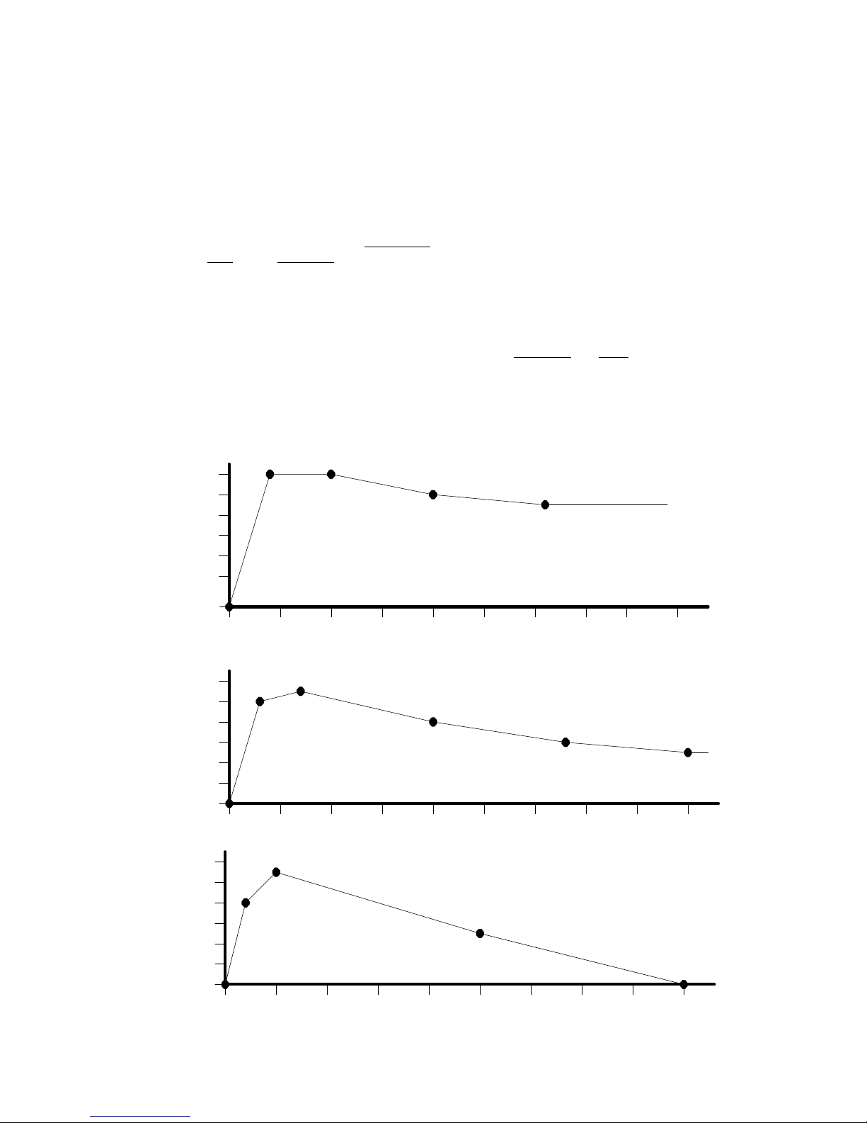
Contours are arbitrarily shaped amplitude envelopes, one for each partial in the model. A contour always starts from silence
(-95.6dB), follows a curve approximated by straight-line segments, and either returns to silence (model of a decaying sound),
ends at some finite value, or loops upon itself (sounds that may be indefinitely sustained). There is no upper limit to the
duration of a contour but accumulated error in generating the contours gives a practical limit in the low minutes range. The
Apple II Sound Modeling Program imposes a limit of 65 seconds.
Contours are effectively represented by a series of breakpoints with straight lines between them. Plotted on a normal graph,
every breakpoint has a time and an amplitude. Amplitude values between breakpoint times lie along a straight line
connecting the breakpoints. Breakpoint times may be unequally and arbitrarily spaced and specified to a precision of 51.2uS.
The breakpoint times of each contour are completely independent and need have no relation with each other. However, voice
memory may be saved and loading of the K150FS’s internal processor reduced if some of the breakpoint times coincide.
Whereas the Sound Modeling Program stores breakpoint data in absolute time (16-bit milliseconds) and amplitude (8-bit
fraction of maximum), breakpoints must be communicated to the K150FS in delta-time
breakpoint is specified relative to the previous breakpoint and the amplitude is specified as the slope of the line segment
connecting to the next breakpoint. Thus everything is relative to the first breakpoint which is always zero time and zero
amplitude. The example below should be studied to understand this.
and slope format. Thus the time of a
Page 3

A data structure for representing all of the contours of a model would normally be a rather complex two-dimensional array
with variable-length rows. Interpreting such an array would involve a lot of searching. For efficiency in playing the
contours, the K150FS requires the breakpoint data to be sorted into a one-dimensional vector of update commands which can
then be interpreted sequentially as time passes. There are four types of commands: Update Slope, Wait, End of Contour, and
End of Note. Note that End of Contour indicates that the partial is no longer needed and thus can be used by some other note.
It should be issued when a partial’s contour has decayed to silence and will remain there. End of Note indicates that no more
commands or arguments are present. The contours not already terminated by End of Contour will continue along whatever
slopes were last specified until the note is actually released. The three contour example above would be encoded into the
update command string listed below.
Command Argument Command Argument Command Argument
UPD#1 2400 dB/s WAIT 30 ms UPD#1 0 dB/s
UPD#2 2667 dB/s UPD#2 -184.6 dB/s WAIT 20 ms
UPD#3 3200 dB/s WAIT 30 ms UPD#2 -48 dB/s
WAIT 20 ms UPD#1 -160 dB/s WAIT 120 ms
UPD#3 1200 dB/s WAIT 100 ms UPD#2 0 dB/s
WAIT 10 ms UPD#1 -72.7 dB/s END#3
UPD#2 200 dB/s UPD#2 -123 dB/s END-0F-NOTE
WAIT 10 ms WAIT 50 ms
UPD#1 0 dB/s UPD#3 -56 dB/s
UPD#3 -240 dB/s WAIT 60 ms
Encoding of the command string above can be accomplished by allocating one byte for the partial number and command
code combined followed by two bytes for the argument. However, since the K150FS’s internal 68000 processor requires 16bit quantities to be at even addresses, the string is split into a command code vector and an argument vector. When a model
is being played, a pointer into each vector is maintained and is incremented to the next element as each element is read. This
makes memory dumps difficult to read but is efficient and compact for the microprocessor. Coding for the command code
bytes is as follows:
CODE ARGUMENT COMMAND MEANING
0 Time Wait Wait before executing next command
0 0 End-of-note No more commands follow
N Slope Update Update partial #N where 1 <= N <= 64
-N none End-of-partial Contour for partial N is complete, can reuse it.
-128 Destination Loopback See below
Actually, there is a fifth type of command; Loopback. This is used for looping contours. The command code byte is $80 (-
128). Its two arguments simply specify how many commands and how many arguments (times 2) the corresponding pointers
must be backed up before continuing. Since all of the contours are encoded into one pair of command and argument strings,
the loop affects all partials which have update commands inside the loop.
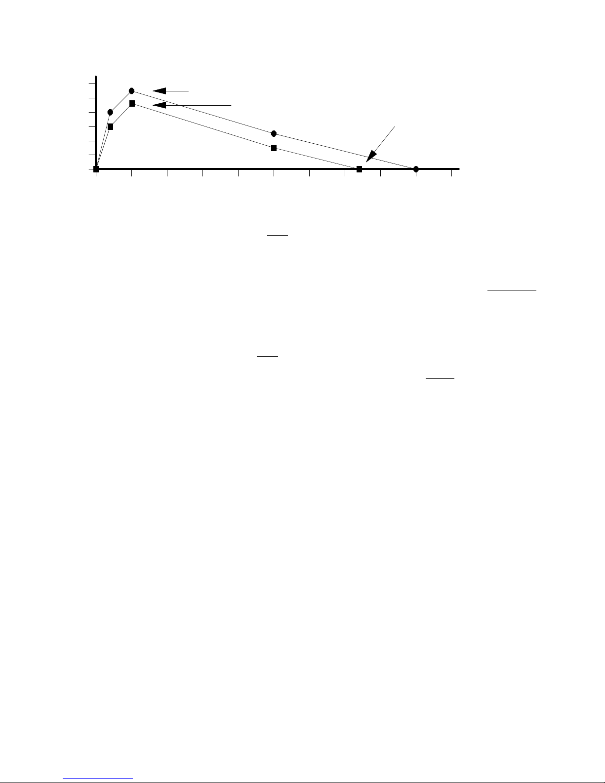
1.3 ATTACK FUNCTION
As mentioned earlier, the first breakpoint of all contours is at zero amplitude and zero time. The second
contour is actually specified by a table called the Attack Function. The third and subsequent breakpoints are specified by the
command and argument lists described above in section 1.2. Since an entire contour in delta-time-slope format is relative to
the amplitude of the second breakpoint, its overall amplitude can be shifted up or down simply by altering the amplitude of
the second breakpoint. This is illustrated below.
breakpoint of each
Page 4
0
-16
-32
-48
-64
-80
-96
dB
0 50 100 150 200 250 300 350 400 450
msec
3200 dB/s
2400 dB/s
30ms
800 dB/s
200ms
-240 dB/s
200ms
-200 dB/s
Original Contour
Second BP shifted
down 16 dB.
Hardware clips
at -95.6 dB
The K150FS operating system considers a host of variables in setting the absolute second breakpoint amplitude of each
partial when a note is started (actually it is setting the slope away from the first breakpoint). These include the attack
function table to be described, the MIDI velocity, the overall loudness of the model, the MIDI volume controller, and the
"graphic equalizer" layer parameters in the sound program. However, once the contours are launched.from the second
breakpoint, their evolution is predestined except for the Release Rates to be discussed later.
The Attack Function is a rectangular array with columns corresponding to partials and rows corresponding to attack levels
.
Each attack level specifies a different spectral modification of the model. A particular attack level is selected according to
the MIDI note-on velocity. There may be as few as one or as many attack levels as desired and they can be arbitrarily
spaced. The entries in this main part of the attack function array are absolute amplitudes of second breakpoints. A zero entry
will suppress the corresponding partial in notes played at the corresponding attack level.
An additional row in the Attack Function gives the times of the second breakpoints, one for each partial (column). An
additional column specifies the MIDI velocity (after translation to amplitude according to the current velocity map) for each
of the attack levels. The last array element at the extra row and column intersection gives the earliest second breakpoint time
which is when interpretation of the update command list should begin.
To make it easier on the processor in the K150FS, the second breakpoint times in the additional row are given as a special
code, not in milliseconds or samples. The codes are drawn from the following table:
TIME CODE TIME CODE TIME CODE TIME CODE TIME CODE
2 53 20 8 55 19 92 30 145 41
3 54 22 9 60 20 95 31 150 42
4 0 25 10 62 21 100 32 160 43
5 55 30 11 65 22 105 33 170 44
6 1 32 12 70 23 110 34 180 45
8 2 35 13 72 24 115 35 190 46
10 3 40 14 75 25 120 36 200 47
12 4 42 15 80 26 125 37 210 48
14 5 45 16 82 27 130 38 220 49
16 6 50 17 85 28 135 39 230 50
18 7 52 18 90 29 140 40 240 51
250 52
Note that only those times listed in the above table are available for the second breakpoint time. The Sound Modeling
Program rounds off the second breakpoint times when a model is compiled but retains millisecond accuracy for the third and
succeeding breakpoints. In cases where the user specified second breakpoint time is greater than 250mS, the .S.M.P.
actually inserts a phantom second breakpoint during compilation at 250mS that resides on the line segment connecting the
user specified first and second breakpoints.
Below is an example of an attack function for the earlier 3 partial example with 3 attack levels. The middle attack level,
which is used when the MIDI velocity maps into a loudness between -12 and -6dB, specifies the model unaltered. The
highest level, used for loudnesses above -6dB, has the first partial left alone but the second boosted by 3dB and the third
boosted by 6dB thus making the sound brighter. The lowest level, used for loudness below -12dB, cuts the third partial by
3dB while leaving the first and second alone.
Page 5

EXAMPLE ATTACK FUNCTION TABLE
Level Partial #l Partial #2 Partial #3
2nd BP time 20 mS 14 11 8
Highest level -6 dB 0 dB -13 dB -26 dB
- - -12 dB 0 dB -16 dB -32 dB
Lowest level -95.6 dB 0 dB -16 dB -35 dB
(Read out row-wise)
1.4 RELEASE SLOPES
Assuming that the Ignore Release model parameter flag is off (see 1.6 below), receipt of a MIDI note-off should cause the
sound to enter its release phase. The release shape of each contour is quite simple: a linear decrease in amplitude from
whatever amplitude the partial was at when the note-off was received to silence. Assuming that the Global Release model
parameter flag is off, each partial can have a different release slope. These slopes are specified in a vector having as many
entries as there are partials. After a note-off, a partial does not become available for reuse by other notes until it has decayed
to silence. An exception would be a restrike of the same note which could immediately reuse its partials.
1.5 UNITS AND ENCODING
The actual binary encoding of the vectors and arrays described above is largely set by the hardware implementation of the
sound generator and to a lesser extent by what is convenient (and therefore fast) for the 68000 control microprocessor. Data
in the arrays are 8 bits in some cases and 16 bits in others. 8-bit quantities are always unsigned integers whereas 16 bit
quantities are always signed, twos-complement integers.
In most cases, the units used to encode time variables into integers are based on the sample rate of the sound generator. This
rate is exactly 19531.25Hz which is exactly equal to a 51.2 uS period. It is derived in the hardware by dividing a 20MHz
clock by 1024. Frequency units are based on the highest standard frequency the sound generator is programmed to produce
which is D9 (A4=440Hz) or 9397.273Hz. Amplitude units are based on a dynamic range of 95.625dB.
1.5.1 Time Units
The Wait command described earlier has a time argument which is a sound generator sample count. It is a signed 16-bit
quantity and thus limited to 32767 which is about 1678 milliseconds. If a wait time longer than this is needed, two or more
Wait commands in a row should be used. In such a string of wait commands, the last one should be checked for very small
values (less than 20). If found, the needed time should be split evenly between the last two Wait commands. For example, if
a wait of 32775 samples is needed, use Wait commands of 16387 and 16388 instead of 32767 and 8.
Time units in the Attack Function table are given in "milliseconds" (the earliest second breakpoint) and codes representing
"milliseconds" (actual second breakpoint times). The "millisecond" units used are actually 1.024 mS long as determined by a
timer chip counting units of 20 samples.
1.5.2 Frequency Units
Frequencies and frequency ratios are always expressed on a log scale which has 2048 integer units per octave. The frequency
of an absolute partial for example is expressed relative to the highest possible frequency of 9397.273Hz. Thus a frequency 3
octaves below this (9397.273 / 8 = 1174.659125Hz) would be expressed as -6144. General conversion formulas are:
Value
= 2954.6394*ln
Hertz
= 9397.273*exp
Hertz
Value
9397.273
2954.6394
( )
( )
Page 6

For relative partials, frequency multiples are expressed using the same 1/2048th octave units. A perfect 4th harmonic, for
example, would be expressed as +4096. General conversion formulas are:
Value
= 2954.6394*ln
Multiple
Note that while frequencies can be specified very precisely with these formulas, the final result produced by the hardware is
quantized to 0.298Hz. This means that even sounds in which perfect harmonic intervals have been specified will generally
not "sit still" on an oscilloscope because the frequency quantization error alters the exact ratios slightly.
For noise partials, the "frequency" field specifies an integer playback rate through the noise table. The two tables are in fact
interleaved in the synthesizer memory and the noise type specification (high/low) simply affects the initial setting of the
noise table pointer to either zero or 4. The spectrum of the noise is defined for a playback rate of 8. Other playback rates
will create different but unpredictable spectra. Note that if the playback rate is not a multiple of 8, samples from the two
tables will be intermixed creating yet another effect. The hardware noise table pointer wraps-a round at 32768 so a playback
rate of 32760 is equivalent to 8 except that the noise table is scanned backward. The relatively short length of the noise table
(4096 samples) limits noise usage to relatively short bursts; otherwise repetition is readily apparent.
1.5.3 Amplitude Units
Where absolute amplitudes are specified, they are represented by an unsigned 8-bit integer in units of 3/8 of a decibel. This
gives a range of 0dB to 95.625dB. In most cases the dB value is an amplitude
maximum loudness. In other cases, the value is an attenuation
generally uses 0dB to represent maximum amplitude and -95.6dB to represent silence.
1.5.4 Slope Units
As described above, contours are represented in the hardware as delta time (sample period counts) and slope. Slopes are
represented by signed 16-bit integers
using the following conversion formulas:
Value
= exp
( )
, so 0 is loud and 255 is silence. The .S.M.P.’s user interface
Multiple
( )
2954.6394
which means that 0 is silence and 255 is
Fast Slope
Value
= 0.034953*(dB/
dB/sec
Note that the relatively large slope unit size restricts usage to fairly rapid slopes. By setting bit 14 of the slope value to one
(after the two’s complement for negative slopes), the slope may be reduced by a factor of 16 and thus slower slopes may be
represented accurately. The conversion formulas are now:
Slow Slope
dB/sec
Slow slopes are accomplished in the hardware by updating the partial amplitude every 16 samples rather than every sample.
This can lead to audible modulation noise if the slow slope flag is on but the slope is relatively fast. Thus judgment in
trading off the greater precision offered by slow slopes with the absence of noise offered by fast slopes must be exercised. In
any case, a routine for converting absolute breakpoints to relative ones for the K150FS should keep track of the errors
incurred and "feed back" a correction to prevent the errors from accumulating. The Apple II .S.M.P. does this and it is
completely effective. The basis of this error feedback process is shown below:
= 28.6098*
Value
= 0.559248*(dB/
= 1.788116*
Value
Value
sec)
sec
)
Page 7

0
-16
dB
300
350 400 450
msec
500 550 600 650
-4
-8
-12
-20
300, -16
600,-20.5
-20.3
550,-9
-7.42
450,-12.5
-13.14
400,-6
-4.56
114.4 dB/s
100 dB/s -171 dB/s
57.2 dB/s
-257.5 dB/s
Actual
Desired
Below is a spreadsheet showing how the values in the example above were calculated:
BREAKPOINT
NUMBER
INITIAL
POINT
DESIRED
ENDPOINT
DESIRED
SLOPE
ACTUAL
SLOPE
ACTUAL
ENDPOINT
1 300,-16 400, -6 100.0 114.4 400, -4.56
2 400, -4.56 450,-12.5 -158.8 -171.7 450,-13.14
3 450,-13.14 550, -9 41.4 57.2 550, -7.42
4 550, -7.42 600,-20.5 -261.6 -257.5 600,-20.30
5 600,-20.30
1.5.5 Partial Phases
No control over the phases of partials is offered by the K150FS. The operating software attempts to set all of the phases to
zero in order to minimize clicks on fast attacks. However, for high frequency partials, delays in getting them started relative
to other partials will result in noticeable (on an oscilloscope) deviations from zero phase. In any case, the 0.298Hz frequency
quantization will generally cause the phases to drift slowly while a note is held, even when exact harmonics are specified.
This effect may be easily seen by playing the built-in sawtooth voice (#253) or generating the .S.M.P. default voice which is
a 16 partial sawtooth. Of course the whole issue of phase is moot for sounds with intended inexact harmonics.
1.6 MODEL PARAMETERS
Model parameters affect the entire sound model in some fashion.
1.6.1 Model Name
The model name is 8 uppercase ASCII characters. Short names may be padded on the right by either blanks or zeroes. Since
we are dealing with models rather than voices, the model name will never appear on the K150FS display and thus serves no
useful purpose except if the model is read back out of the K150FS’s voice RAM.
1.6.2 Highest Note
When two or more models are combined into a voice, this parameter specifies the highest MIDI note number the model can
play. The lowest note is one higher than the highest note of the previous model. The first model however can play down to
C0 while the last model can play up to C8 regardless of this parameter.
1.6.3 Ignore Release Flag
For a sound that must play its contours to the end regardless of when the MIDI note-off is received (example: undamped
bell), this flag should be set. To avoid an abrupt termination of partials when the End-of-Note command is reached, they
should all have decayed to silence first. With this flag set, release slopes have no meaning since there is no release. This flag
should not be set if a Loopback command is present; if it is, End-of-Note will never be reached and the contours will loop
forever.
Page 8

1.6.4 Hold at End Flag
For a sustained sound (example: horn) that must last as long as the key is held, this flag is set to prevent the End-of-Note
command from shutting off all of the partials when it is reached. Note that Ignore Release and Hold at End should not both
be set; if they are, the note will hang on forever. The setting of this flag is irrelevant if a Loopback command is present since
End-of-Note will never be reached.
1.6.5 Global Release Flag
If this flag is set, a single release slope value given elsewhere in the model specifies the release slops of all of the partials. If
it is not set, a vector gives independent release slopes for each partial.
1.6.6 Ignore Sustain Pedal
This flag does what its name implies. The Apple II .S.M.P. has no way to set this flag.
1.6.7 Attenuation
This 8-bit unsigned value determines how loud the overall model is in units of 3/8dB. A value of 0 specifies maximum
possible loudness. The user would typically adjust this value so that the subjective loudness of the model balances that of
other models and voices.
1.7 COMPLETE MODEL STRUCTURE
The listing below gives the memory image of the example model that has been used previously. Encoding of the memory
image into a system exclusive MIDI message is covered in section 2. Note that bit 0 is the least significant bit and that 16-bit
quantities have the most significant byte at the lower (even) address. The symbolic names given to the various fields come
from the Apple II version of the .S.M.P. and are shown here simply as mnemonic aids. To make reading easier, decimal
values are given with no prefix and hex values have a $ prefix.
MODELH Beginning of a model header
MHNAME .BYTE ’ABCDEFGH’ 8 Character uppercase model name in ASCII
MHKEY .BYTE 72 Highest MIDI key number for the model (C5)
MHFLAGS .BYTE $00 Model option flags
Bit 0: 1=Ignore release
1: 1=Global release slope
2: 0 always
3: 1=Ignore sustain pedal
4: 1=Hold at end
5-7: 0 always
MHNPART .BYTE 3 Number of partials (1-64)
MHNAFLV .BYTE 3 Number of Attack Function LEVELS (1-254)
MHNUPDC .WORD 24 Number of Update COMMANDS
MHNUPDA .WORD 23 Number of Update ARGUMENTS
MHOFPFG .WORD PFGLIST-MODELH (48) Offset to partial flags list
MHOFPFQ .WORD PFQLIST-MODELH (52) Offset to partial frequency list (EVEN)
MHOFATF .WORD PAFLIST-MODELH (58) Offset to attack function array
MHOFUPC .WORD PUCLIST-MODELH (74) Offset to update commands list
MHOFUPA .WORD PUALIST-MODELH (98) Offset to update arguments list (EVEN)
MHOFIRR .WORD PRSLIST-MODELH (144) Offset to release slope list, if individual (EVEN);
actual release slope if global
MHLOUD .BYTE 8 Attenuation of the model (-3dB)
DS.B 19 19 bytes unused (set to zero)
NOTE: These lists need not directly follow the model header, nor be in the order shown below, as long as the offsets given
in the model header are accurate.
PFGLIST .BYTE $00 List of partial flags, one byte per partial
.BYTE $00 $00=relative, $01=absolute, $03=low noise,
.BYTE $00 $07=high noise, add $10 to mark optional
Page 9

PFQLIST .WORD 0 1.000* List of partial frequencies
.WORD 2048 2.000* (multiples for relative partials)
.WORD 3246 3.000*
PAFLIST .BYTE 20 Earliest second breakpoint time in actual mS
.BYTE 14,11,8 CODES for second breakpoint times of 3 partials
.BYTE 16 Amplitude defining highest attack level (-6dB)
.BYTE 255,220,185 Corresponding second breakpoint amplitudes
.BYTE 32 Amplitude defining mid attack level (-12dB)
.BYTE 255,212,170 Corresponding second breakpoint amplitudes
.BYTE 255 Amplitude defining lowest attack level (-95.6dB)
.BYTE 255,212,162 Corresponding second breakpoint amplitudes
PUCLIST .BYTE 3 Update #3, 772.5dB/S
.BYTE 0 Wait 10mS
.BYTE 2 Update #2, 171.7dB/S
.BYTE 0 Wait 10mS
.BYTE 1 Update #I, 0dB/S
.BYTE 0 Wait 10mS
.BYTE 3 Update #3, -228.9dB/S
.BYTE 0 Wait 20mS
.BYTE 2 Update #2, -171.7dB/S
.BYTE 0 Wait 30mS
.BYTE 1 Update #1, -143.0dB/S
.BYTE 0 Wait 100mS
.BYTE 1,2 Update #I, -80.5dB/S; Update #2, -114.4dB/S
.BYTE 0 Wait 50mS
.BYTE 3 Update #3, -200.3dB/S
.BYTE 0 Wait 60mS
.BYTE 1 Update #1, 0dB/S
.BYTE 0 Wait 20mS
.BYTE 2 Update #2, -84dB/S
.BYTE 0 Wait 120mS
.BYTE 2 Update #2, 0dB/S
.BYTE -3 End #3 (no argument)
.BYTE 0 End-of-Note
PUALIST .WORD 27 Update #3, 772.5dB/S
.WORD 195 Wait 10mS
.WORD 6 Update #2, 171.6dB/S
.WORD 195 Wait 10mS
.WORD 0 Update #I, 0dB/S
.WORD 195 Wait 10mS
.WORD -8&$BFFF Update #3, -228.9dB/S
.WORD 390 Wait 20mS
.WORD -6&$BFFF Update #2, -171.7dB/S
.WORD 585 Wait 30mS
.WORD -5&$BFFF Update #1, -143.0dB/S
.WORD 1952 Wait 100mS
.WORD -45 Update #I, -80.5dB/S (Slow slope)
.WORD -4&$BFFF Update #2, -114.4dB/S
.WORD 976 Wait 50mS
.WORD -7&$BFFF Update #3, -200.3dB/S
.WORD 1171 Wait 60mS
.WORD 0 Update #1, 0dB/S
.WORD 390 Wait 20mS
.WORD -47 Update #2, -84.0dB/S (Slow slope)
.WORD 2343 Wait 120mS
Page 10

.WORD 0 Update #2, 0dB/S
.WORD 0 End-of-Note
PRSLIST .WORD -20 Release slope for 1st partial(slow, -35.8dB/sec)
.WORD -40 2nd partial (slow, -71.5dB/sec)
.WORD -5&$BFFF 3rd partial (fast, -143.0dB/sec)
1.8 VOICE STRUCTURE
Actually, individual sound models are not sent to the K150FS, only complete voices. A voice is made of 1 or models in
ascending pitch range sequence. When the .S.M.P. sends a single model to the K150FS for auditing, it is first assembled
into a single model voice. The structure of a complete voice is shown schematically below:
VOICE HEADER (32 bytes)
MODEL HEADER (lowest pitch range, 48 bytes)
- - MODEL HEADER (highest pitch range, 48 bytes)
DATA ARRAYS FOR THE MODELS (order not important)
All of the model headers must follow the voice header. A field in the voice header specifies how many models follow so the
K150FS knows when it reaches the end of the model header list. The data arrays follow the model headers. They can be in
any sequence desired so long as the offset fields in the corresponding model headers point to them. Note that each offset is
relative to the beginning of the associated model header.
The format of the voice header is as follows:
VOICER
VHNAME .BYTE ’ABCDEFGH’ 8 character uppercase voice name in ASCII
VHNUMBR .BYTE 200 Voice ID number in K150FS
VHNMDLS .BYTE 6 Number of models in the voice
DS.B 22 22 bytes for expansion, make zero
The voice ID number is how voices are referred to in the K150FS sound program editing system. Generally, numbers greater
than 100 should be used to prevent conflict with the built-in ROM voices.
Page 11

2. SYSTEM EXCLUSIVE MESSAGE FORMAT
Exchange of non-musical data such as voices and remote front panel programming is accomplished via MIDI SystemExclusive messages. The K150FS message system uses a closed-loop handshaking protocol to regulate the flow of systemexclusive data. The formats of the messages and the protocol are described below.
2.1 MESSAGE HEADER
Every system-exclusive message, in either direction, consists of a header, optional data, and MIDI EOX status code ($F7). A
message thus consists of the following bytes:
$F0 MIDI system-exclusive status code
$07 Kurzweil ID code
sel Device Select. For several identical units connected together, specifies which one should respond.
Range is $00-$0F and for K150FS, the device ID is the same as the basic MIDI channel.
$0F Product code for K150FS
cc Command/status code (see list below)
data optional
$F7 MIDI end-of-exclusive
COMMAND/STATUS CODES MEANING
$01
$02
$03
$04
$05
$06
$07
$08
$09
$0A
$7E
$7F
Only Dump Voice, Load Voice, Block Data Transfer, NAK, and ACK are described in this document. The others are
described in a document titled: "K150FS Version 1.6 Software" (applies to 1.7 and later versions as well).
Load master parameter block
Dump master parameter block
Load program
Dump program
Load voice
Dump voice
Block data transfer
Remote button push
Request display content
Display text (acknowledgment to $09)
NAK (negative acknowledge; error)
ACK (positive acknowledge; OK)
2.2 ENCODING OF 8-BIT BINARY DATA
The data portion, if present, of messages usually consists of full 8-bit bytes. These are sent as pairs of MIDI bytes, 4 bits for
each member of the pair. The most significant 4 bits are sent first. Thus the MIDI bytes $4D $69 $64 $69 would be sent as
$04 $0D $06 $09 $06 $04 $06 $09. Although other packing techniques may be more efficient, this simple method is human
readable from a MIDI data logger and quite efficient enough for the relatively small amount of data required to represent
additive synthesis sounds.
2.3 HANDSHAKING PROTOCOL
The K150FS is connected to a computer with two MIDI cables. One connects the computer’s MIDI output to the K150FS
MIDI input and the other connects the K150FS MIDI output to the computer’s MIDI input. Note that the K150FS MIDI
output does not
Different message types use different protocols. The protocol for messages associated with voice loading dumping are
described below. Protocols for the other message types are outlined in K150FS Version 1.6 Software.
retransmit the normal musical messages it receives; it is only used to reply to system-exclusive messages.
Page 12

2.4 SENDING A VOICE
To send a voice to the K150FS, the host computer program must follow these steps in sequence:
1. Determine how large the voice will be inclusive of data and all headers.
2. Send a Load Voice command ($05 command code) system-exclusive message to the K150FS. The data field of the
message is as follows (each byte is two nybbles):
.BYTE vnum Voice number
.WORD size Voice size
3. Wait for a reply message from the K150FS. It will be an ACK if there is sufficient free space in voice RAM to hold the
voice, otherwise it will be a NAK. If no response is received within a second, there is a communication problem.
4. Assuming an ACK was received, send a Block Data command ($07). The data field is the complete voice beginning
with the first byte of the voice header using the two nybble per byte encoding method. Note that the voice ID number
given in the voice header must agree with the number given in the Load Voice command in step 2.
5. Wait for a reply message from the K150FS. It will be an ACK if no gross errors are found in the voice data (such as an
odd number of data nybbles). Otherwise it will a NAK. Only the simplest errors are checked for. Erroneous voice data
will likely cause the K150FS software to crash when a key is played. Again, if there is no reply within one second of
sending the last data byte, there is a communication problem.
2.5 RECEIVING A VOICE
Voice data from the built-in factory sound ROMs or previously loaded data in the sound RAM can be read back from the
K150FS. To read voice information, the host computer must do the following steps:
Send a Dump Voice command (code $06). The data field is as follows:
.BYTE vnum Voice number to dump, two nybble format
.BYTE type Modifier, a single MIDI byte interpreted as follows:
$00 = Send headers only (voice then model headers)
NN = Send model N (1=first=lowest, etc.).
Data will be a voice header, one model header, corresponding model data.
$7F = Send whole voice (all headers plus all data)
Wait for a Block Data message in response. If a NAK is received instead, then the voice number requested doesn’t exist.
The format of the headers and the data arrays is the same as described in Section 1 above. Note that some of the unused
fields in the headers may contain data other than zeroes; this is not significant.
 Loading...