HP HPjmete User Manual

HPjmeter 4.2 User's Guide

HP Part Number: 5900-2022
Published: December 2011
Edition: 1

© Copyright 2005-2011 Hewlett-Packard Development Company, L.P.

Document Notice

The information in this document is subject to change without notice.

Hewlett-Packard makes no warranty of any kind with regard to this manual, including, but not limited to, the implied warranties of merchantability and fitness

for a particular purpose. Hewlett-Packard shall not be held liable for errors contained herein or direct, indirect, special, incidental, or consequential

damages in connection with the furnishing, performance, or use of this material.

Warranty

A copy of the specific warranty terms applicable to your Hewlett-Packard product and replacement parts can be obtained from your local Sales

and Service Office.

U.S. Government License

Proprietary computer software. Valid license fromHP required for possession, use or copying.Consistent with FAR 12.211 and 12.212,Commercial

Computer Software, Computer Software Documentation, and Technical Data for Commercial Items are licensed to the U.S. Government under

vendor's standard commercial license.

You can find printable PDF versions of this user's guide and the release notes in the installation directory (doc subdirectory).

Copyright Notices

© Copyright 2005–2011 Hewlett-Packard Development Company, L.P. All rights reserved. Reproduction, adaptation, or translation of this

document without prior written permission is prohibited, except as allowed under copyright laws.

Trademark Notices

This product includes software developed by the Apache Software Foundation (http://www.apache.org/).

Intel and Itanium are trademarks or registered trademarks of Intel Corporation or its subsidiaries in the United States and other countries.

Microsoft and Windows are U.S. registered trademarks of Microsoft Corporation.

UNIX is a registered trademark of The Open Group.

Java™ and all Java based trademarks and logos are trademarks or registered trademarks of Oracle and/or its affiliates in the United States and

other countries.

HP-UX Release 11i and later (in both 32- and 64-bit configurations) are Open Group UNIX 95 branded products.

Table of Contents

About This Document.......................................................................................................10

Intended Audience................................................................................................................................10

Typographic Conventions.....................................................................................................................10

Additional HPjmeter Documents.........................................................................................................10

Related Information..............................................................................................................................10

Publishing History................................................................................................................................11

HP Encourages Your Comments..........................................................................................................11

1 Introducing HPjmeter 4.2.00.00 ...............................................................................12

Features.................................................................................................................................................12

Concepts................................................................................................................................................13

JVM Agent.......................................................................................................................................13

Node Agent.....................................................................................................................................13

2 Completing Installation of HPjmeter .........................................................................14

Platform Support and System Requirements.......................................................................................14

Agent Requirements........................................................................................................................14

Console Requirements.....................................................................................................................14

Completing the installation..................................................................................................................15

File Locations........................................................................................................................................15

Attaching to the JVM Agent of a Running Application.......................................................................15

Configuring your Application to Use HPjmeter Command Line Options..........................................15

Preparing to run Java.......................................................................................................................15

Example Usage...........................................................................................................................16

JVM Agent Options.........................................................................................................................17

Showing Version Information....................................................................................................17

Selecting Other JVM Agent Options..........................................................................................17

JVM Options Usage Examples...................................................................................................21

Security Awareness...............................................................................................................................21

Securing Communication Between the HPjmeter Node Agent and the Console...........................21

Ensuring the Integrity of HPjmeter Console/Node Agent Data Transfer..................................21

Protecting Data Confidentiality During HPjmeter Console/Node Agent Communication......21

Working with Firewalls .............................................................................................................21

Configuring User Access............................................................................................................22

Securing Communication Between the JVM and the HPjmeter Node Agent ................................22

3 Getting Started ............................................................................................................23

Are You Monitoring an Application or Analyzing Collected Data?....................................................23

Using HPjmeter to Monitor Applications.............................................................................................23

Configure and Start Your Application............................................................................................23

Confirm that the Node Agent is Running.......................................................................................23

Start the Console..............................................................................................................................23

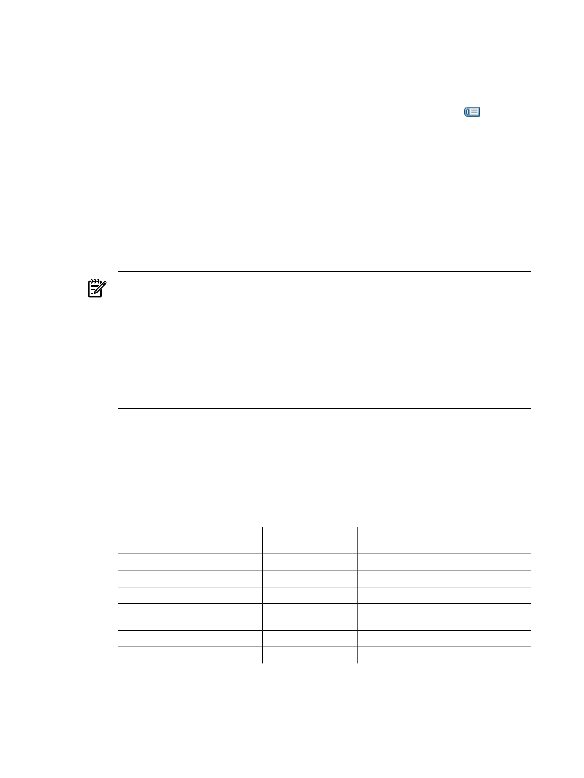
Connect to the Node Agent from the Console................................................................................23

Set Session Preferences....................................................................................................................26

Changing Session Preferences During a Session.............................................................................29

View Monitoring Metrics During Your Open Session....................................................................29

Using HPjmeter to Analyze Profiling Data..........................................................................................29

Using HPjmeter to Analyze Garbage Collection Data.........................................................................31

Monitoring Demonstration Instructions...............................................................................................32

Memory Leak Applications.............................................................................................................33

Thread Deadlock Sample.................................................................................................................34

Table of Contents 3

4 Monitoring Applications ............................................................................................36

Controlling Data Collection and Display.............................................................................................36

Setting Data Collection Preferences......................................................................................................36

Managing Node Agents........................................................................................................................37

Managing Node Agents On HP-UX................................................................................................37

Running Node Agent as a Daemon...........................................................................................37

Verifying HP-UX Daemon is Running.......................................................................................37

Starting Node Agents Manually................................................................................................37

Stopping Node Agents...............................................................................................................38

Node Agent Access Restrictions......................................................................................................38

Running Multiple Node Agents......................................................................................................38

Saving Monitoring Metrics Information...............................................................................................38

Saving Data from the Console.........................................................................................................39

Naming Monitoring Data Files.............................................................................................................39

Diagnosing Errors When Monitoring Running Applications..............................................................39

Identifying Unexpected CPU Usage by Method.............................................................................39

Viewing the Application Load........................................................................................................40

Checking for Long Garbage Collection Pauses...............................................................................40

Checking for Application Paging Problems....................................................................................40

Identifying Excessive Calls to System.gc()......................................................................................41

Reviewing the Percentage of Time Spent in Garbage Collection....................................................41

Checking for Proper Heap Sizing....................................................................................................43

Confirming Java Memory Leaks......................................................................................................43

Determining the Severity of a Memory Leak..................................................................................43

Identifying Excessive Object Allocation..........................................................................................44

Identifying the Site of Excessive Object Allocation.........................................................................44

Identifying Abnormal Thread Termination....................................................................................44

Identifying Multiple Short-lived Threads.......................................................................................44

Identifying Excessive Lock Contention...........................................................................................45

Identifying Deadlocked Threads.....................................................................................................45

Identifying Excessive Thread Creation...........................................................................................45

Identifying Excessive Method Compilation....................................................................................46

Identifying Too Many Classes Loaded............................................................................................47

Using the JMX Viewer...........................................................................................................................47

Understanding the JMX Summary View.........................................................................................48

JMX Summary Tab.....................................................................................................................48

JMX Memory Tab.......................................................................................................................49

JMX Threads Tab........................................................................................................................51

JMX Runtime Tab.......................................................................................................................52

JMX Notifications Tab................................................................................................................52

Changing Mbean Values and Monitoring the Result......................................................................52

Using the Functions in the JMX Server View..................................................................................53

The MBean Filter........................................................................................................................53

The MBean Attribute Tab...........................................................................................................54

The MBean Operations Tab........................................................................................................55

The MBean Notifications Tab.....................................................................................................56

The MBean Information Tab......................................................................................................56

5 Profiling Applications .................................................................................................58

Profiling Overview................................................................................................................................58

Tracing.............................................................................................................................................59

Sampling..........................................................................................................................................59

Tuning Performance........................................................................................................................59

Preparing a Benchmark........................................................................................................................60

Collecting Profile Data..........................................................................................................................61

4 Table of Contents

Profiling with -Xeprof......................................................................................................................61

Profiling with Zero Preparation......................................................................................................62

Profiling with -agentlib:hprof..........................................................................................................63

Naming Profile Data Files...............................................................................................................65

–Xeprof and –agentlib:hprof Profiling Options and Their Corresponding Metrics.............................65

Approaches to Analyzing Performance Data.......................................................................................68

Looking at the Data from the Bottom Up........................................................................................68

Looking at the Data from the Top Down........................................................................................68

Looking for Inefficiencies in Memory Usage..................................................................................68

Considerations in Interpreting the Data...............................................................................................68

Inclusive Versus Exclusive Time.....................................................................................................69

Time Units.......................................................................................................................................69

CPU Versus Clock Time.............................................................................................................69

Locating Summary Information for Saved Data Sets...........................................................................69

Adjusting Scope....................................................................................................................................70

Comparing Profiling Data Files ...........................................................................................................71

Scaling Comparison Data.....................................................................................................................72

Reading Profiling Histograms..............................................................................................................73

Key to Thread States Reported by ..................................................................................................73

Interpreting the Histogram Presentation........................................................................................74

Using Call Graph Trees.........................................................................................................................75

Interpreting Call Graph Data..........................................................................................................75

Example of Node Color Display................................................................................................76

Options for Manipulating the Call Tree Display.............................................................................77

Tree Pruning...............................................................................................................................77

Auto-Expanding the Call Tree...................................................................................................77

Using Sub-Trees..........................................................................................................................77

Searching the Trees.....................................................................................................................78

Using Heuristics to Locate Possible Hot Spots.....................................................................................78

6 Analyzing Garbage Collection Data .......................................................................80

Obtaining Garbage Collection Data......................................................................................................80

Data Collection with -Xverbosegc...................................................................................................80

Collecting Allocation Site Statistics for Viewing in HPjmeter...................................................83

Collecting Glance Data for Viewing in HPjmeter......................................................................83

Collecting GC Data with Zero Preparation.....................................................................................83

Data Collection with -Xloggc...........................................................................................................84

Naming GC Data Files.....................................................................................................................85

-Xverbosegc and -Xloggc Options and Their Corresponding Metrics.................................................85

Locating Summary Information for Saved Data Sets...........................................................................86

Comparing Garbage Collection Data Files ..........................................................................................86

Basic Garbage Collection Concepts......................................................................................................87

Key to Garbage Collection Types Recognized by HPjmeter...........................................................87

Understanding the Summary Presentation of GC Data..................................................................88

Understanding the System Details Captured with GC Data..........................................................90

7 Using the Console .......................................................................................................93

Starting the Console..............................................................................................................................93

Starting the Console On HP-UX......................................................................................................93

Starting the Console On Linux........................................................................................................93

Starting the Console On Microsoft Windows..................................................................................93

Using the Main Window Functions......................................................................................................93

Data Representation........................................................................................................................94

Icons and Their Meaning.................................................................................................................95

Node Agent................................................................................................................................95

JVM Agent..................................................................................................................................95

Table of Contents 5

Open and Cached Sessions........................................................................................................96

Time Slice Entries.......................................................................................................................96

Saving Data................................................................................................................................96

Console Tool Bar Buttons................................................................................................................97

Console Menu Choices....................................................................................................................97

The Monitor Menu.....................................................................................................................98

Console Guide.................................................................................................................................99

Status Bar.......................................................................................................................................100

Setting Monitoring Session Preferences .............................................................................................100

Specifying Metrics to Collect for Monitoring................................................................................100

Enabling Monitoring Alerts...........................................................................................................101

Specifying Filters for Monitoring .................................................................................................102

Editing Filters...........................................................................................................................102

Adding Filters...........................................................................................................................102

Specifying Filter Sets................................................................................................................103

Viewing Monitoring Data in HPjmeter...............................................................................................103

Using Alerts........................................................................................................................................103

Using the Alert Controller.............................................................................................................105

Viewing a Log of the Alert History..........................................................................................107

Editing E-mail Notification Attributes..........................................................................................107

Responding to Alerts.....................................................................................................................108

Abnormal Thread Termination Alert.......................................................................................108

Uncaught Exception Statistics.............................................................................................109

Excessive Compilation Alert....................................................................................................110

Expected Out Of Memory Error Alert......................................................................................110

GC Duration Notification.........................................................................................................110

Heap Usage Notification..........................................................................................................111

Java Collection Leak Locations Alert.......................................................................................111

Array Leak Locations Alert......................................................................................................112

Process CPU Usage Alert.........................................................................................................113

System CPU Usage Alert..........................................................................................................114

Thread Deadlock Alert.............................................................................................................115

Unfinalized Queue Growth......................................................................................................115

8 Using Visualizer Functions .......................................................................................116

Visualizer Behavior When Monitoring Behavior or Analyzing Data.................................................116

Locating Information About a JVM and its Environment..................................................................117

Using Monitoring Displays.................................................................................................................117

Monitor Code and/or CPU Activity Menu....................................................................................118

Java Method HotSpots..............................................................................................................118

Guidelines...........................................................................................................................119

Details..................................................................................................................................119

Thrown Exceptions...................................................................................................................120

Thrown Exceptions with Stack Traces......................................................................................120

Monitor Memory and/or Heap Activity Menu.............................................................................122

Heap Monitor...........................................................................................................................122

Guidelines...........................................................................................................................122

Details..................................................................................................................................123

Garbage Collections..................................................................................................................123

Guidelines...........................................................................................................................124

Details..................................................................................................................................124

GC Duration.............................................................................................................................124

Guidelines...........................................................................................................................124

Details..................................................................................................................................125

Percentage of Time Spent in Garbage Collection.....................................................................125

6 Table of Contents

Guidelines...........................................................................................................................125

Details..................................................................................................................................125

Unfinalized Objects..................................................................................................................126

Guidelines...........................................................................................................................126

Details..................................................................................................................................126

Allocated Object Statistics by Class..........................................................................................127

Guidelines...........................................................................................................................127

Details..................................................................................................................................127

Allocating Method Statistics.....................................................................................................128

Guidelines...........................................................................................................................128

Details..................................................................................................................................128

Current Live Heap Objects.......................................................................................................129

Details..................................................................................................................................130

Monitor Threads and/or Locks Menu............................................................................................131

Thread Histogram....................................................................................................................131

Guidelines...........................................................................................................................132

Details..................................................................................................................................132

Lock Contention.......................................................................................................................133

Guidelines...........................................................................................................................133

Details..................................................................................................................................133

Monitor JVM and/or System Activity Menu.................................................................................134

Method Compilation Count.....................................................................................................134

Guidelines...........................................................................................................................134

Method Compilation Frequency..............................................................................................135

Guidelines...........................................................................................................................135

Loaded Classes.........................................................................................................................135

Guidelines...........................................................................................................................135

Percent (%) CPU Utilization.....................................................................................................136

Guidelines...........................................................................................................................136

Viewing Profiling or GC Data in HPjmeter........................................................................................137

Using Profile Displays.........................................................................................................................137

Menu Choices................................................................................................................................140

Profile Code and/or CPU Activity.................................................................................................140

Method Call Count...................................................................................................................140

Exclusive Method Times (CPU)...............................................................................................141

Exclusive Method Clock Times................................................................................................141

Call Graph Tree with Call Count..............................................................................................141

Call Graph Tree with CPU........................................................................................................142

Call Graph Tree with Clock Time.............................................................................................142

Inclusive Method CPU Times...................................................................................................142

Inclusive Method Clock Times.................................................................................................142

Average Exclusive Method CPU Times*..................................................................................142

Average Exclusive Method Clock Times*................................................................................143

Average Inclusive Method CPU Times*...................................................................................143

Average Inclusive Method Clock Times*.................................................................................143

Starvation by Method*..............................................................................................................143

Starvation Ratio*.......................................................................................................................144

Methods with Loops*...............................................................................................................144

Exclusive Class CPU Times*.....................................................................................................144

Exclusive Class Clock Times*...................................................................................................144

Profile Memory and/or Heap Activity..........................................................................................144

Objects Created by Method......................................................................................................145

Created Objects (Count)...........................................................................................................145

Created Objects (Bytes)............................................................................................................145

Live Objects (Count).................................................................................................................145

Table of Contents 7

Live Objects (Bytes)..................................................................................................................145

Live Array Sizes........................................................................................................................145

Unfinalized Objects..................................................................................................................146

Reference Graph Tree...............................................................................................................146

Reference Sub-Trees by Size.....................................................................................................146

Object and Primitive Value Tables......................................................................................147

Related Topics.....................................................................................................................149

Class Loaders............................................................................................................................150

Guidelines...........................................................................................................................151

Residual Objects (Count)..........................................................................................................152

Residual Objects (Bytes)...........................................................................................................152

Profile by Threads..........................................................................................................................152

Threads Histogram...................................................................................................................152

Thread Groups Histogram.......................................................................................................153

Profile by Locks.............................................................................................................................153

Contested Lock Claims by Method..........................................................................................154

All Lock Claims by Method.....................................................................................................154

Lock Delay - Method Exclusive................................................................................................154

Lock Delay - Call Graph Tree...................................................................................................154

Lock Delay - Method Inclusive................................................................................................155

Lock Contention Ratio by Method*..........................................................................................155

Average Exclusive Method Lock Delay*..................................................................................155

Exclusive Method Lock Delay / Clock Time*...........................................................................155

Average Inclusive Method Lock Delay*...................................................................................155

Inclusive Method Lock Delay / Clock Time*............................................................................155

Exclusive Class Lock Delay*.....................................................................................................156

Using Heuristic Metrics from the Estimate Menu.........................................................................156

Inline Candidates.....................................................................................................................156

Exceptions Thrown...................................................................................................................156

Memory Leaks..........................................................................................................................156

Using Specialized Garbage Collection Displays.................................................................................157

Heap Usage After GC....................................................................................................................157

Duration (Stop the World).............................................................................................................158

Cumulative Allocation...................................................................................................................159

Creation Rate.................................................................................................................................160

Allocation Site Statistics.................................................................................................................161

How a Snapshot of Allocation Sites Statistics is Shown in GC Visualizers.............................166

User-Defined X-Y Axes..................................................................................................................167

Multiple User-Defined...................................................................................................................168

Glance Data....................................................................................................................................170

Glance System Call Data................................................................................................................174

Using Visualizer Tool Bars..................................................................................................................176

Common Tool Bar Buttons.............................................................................................................176

Tool Bar Buttons for Manipulating Tabular Data..........................................................................177

Tool Bar Buttons for Manipulating Graphical Data......................................................................177

Tool Bar Buttons for Manipulating Garbage Collection Data..................................................177

Special Button or Other Gadget Functions....................................................................................178

Mark an Item for Search...........................................................................................................178

Using the Marked Object List on the Console....................................................................179

Find a Search Pattern................................................................................................................179

Editing the Finder...............................................................................................................181

Pause or Resume Graphical Time-based Scrolling...................................................................181

Changing Time Interval in GC Data Visualizers......................................................................181

Select a Subset of the Available Data..................................................................................181

Apply Selected Interval Across All Metrics........................................................................183

8 Table of Contents

Reset Interval to Default Settings Across All Metrics.........................................................184

Changing Time Interval in Monitoring Visualizers.................................................................184

Change Color Selection for Histogram Display..................................................................................185

9 Understanding How HPjmeter Works ....................................................................187

Performance Overhead on Running Applications..............................................................................187

Application Server Startup Time...................................................................................................187

Monitoring Overhead....................................................................................................................187

Changes in Memory Overhead With Dynamic Attach............................................................187

Profiling Overhead and Intrusion.................................................................................................187

Node Agent Overhead...................................................................................................................187

Console Overhead..........................................................................................................................188

Data Sampling Considerations...........................................................................................................188

Using Confidence Interval to Indicate Sample Validity................................................................188

How Memory Leak Detection Works.................................................................................................189

Tapping in to Standard Management of the Java Virtual Machine....................................................190

10 Troubleshooting ......................................................................................................192

Documentation and Support..............................................................................................................192

Identifying Version Numbers.............................................................................................................192

Installation...........................................................................................................................................192

Console ...............................................................................................................................................193

JVM agent............................................................................................................................................194

Node agent..........................................................................................................................................195

Zero Preparation Profiling..................................................................................................................195

Unexpected Behavior in Visualizers...................................................................................................196

A Quick References.......................................................................................................197

Connecting to the HPjmeter Node Agent...........................................................................................197

Determining Which HPjmeter Features Are Available With a Specific JVM Version........................197

Default Location of Xverbosegc and Allocation Site Statistics Data Files..........................................198

Glossary ........................................................................................................................199

Index...............................................................................................................................202

Table of Contents 9

About This Document

This document provides updated information about product features, known problems, and
workarounds for the 4.2 release of HPjmeter.

Intended Audience

This document is intended for application administrators and software developers responsible
for monitoring Java application performance and operation on HP-UX. Users are expected to
have some knowledge of concepts and/or commands for the HP-UX operating system, usage of
the Java Virtual Machine on HP-UX, and Java application performance. When running the
HPjmeter console on a Microsoft® Windows® platform, the user is expected to be familiar with
installing executables and navigating the Windows file system.

Typographic Conventions

This document uses the following typographical conventions.
audit(5) A man page. The man page name is audit, and it is located in Section 5.

Command

ComputerOut

ENVIRONVAR The name of an environment variable, for example, PATH.

[ERRORNAME]

A command name or qualified command phrase.

Text displayed by the computer.

The name of an error, usually returned in the errno variable.

Key The name of a keyboard key. Return and Enter both refer to the same key.

UserInput

Variable

... The preceding element can be repeated an arbitrary number of times. A vertical

| Separates items in a list of choices.

Commands and other text that you type.

The name of a placeholder in a command, function, or other syntax display
that you replace with an actual value.

ellipsis indicates the continuation of a code example.

Additional HPjmeter Documents

• HPjmeter 4.2.00.00 Release Notes and Installation Guide: http://www.hp.com/go/

hpux-hpjmeter-docs.

• HPjmeter overview and access to software: https://h20392.www2.hp.com/portal/swdepot/

displayProductInfo.do?productNumber=HPJMETER .

Related Information

• JSR 174: Monitoring and Management Specification for the Java™ Virtual Machine at Java
Community Process web site: http://www.jcp.org/en/jsr/detail?id=174

• Java™ Troubleshooting Guide for HP-UX Systems: http://www.hp.com/go/hpux-java-docs

• Patch Information for Java on HP-UX: http://ftp.hp.com/pub/softlib/hpuxjava-patchinfo/

index.html

• HP-UX Secure Shell Getting Started Guide: http://www.hp.com/go/hpux-security-docs

• HP-UX System Administrator's Guide: Security Management, “Securing Remote Sessions Using
HP-UX Secure Shell” : http://www.hp.com/go/hpux-core-docs-11iv3

• Memory Management in the Java HotSpot™ Virtual Machine (Sun Developer Network): http://

java.sun.com/j2se/reference/whitepapers/memorymanagement_whitepaper.pdf

Publishing History

The document publication date and part number indicate this document's current edition. The
publication date changes when a new edition is printed. Document updates may be issued
between editions to correct errors or document product changes. To ensure that you receive the
updated or new editions, subscribe to the appropriate product support service. See your HP
sales representative for details. You can find the latest version of this document on the HP Business
Support Center at http://www.hp.com/go/hpux-hpjmeter-docs.

Publication DateEdition NumberSoftware Version NumberHP Part Number

December 201114.2.00.005900-2022

September 201014.1.00.005900-1025

May 200914.0.00.005992-5899

June 200813.1.0.005992-0757

November 200613.0.0.005991-6757

September 200622.15991-6686

July 200612.15991-5846

February 200612.05991-5437

HP Encourages Your Comments

We encourage your comments concerning this document. We are committed to providing
documentation that meets your needs.

Please send your comments via the Customer Feedback web page: http://www.hp.com/bizsupport/

feedback/ww/webfeedback.html. Include the document title, HP part number, and any comment,

error found, or suggestion for improvement you have concerning this document. Also, please
let us know what we did right so we can incorporate it into other documents.

1 Introducing HPjmeter 4.2.00.00

HPjmeter is a performance analysis tool for deployed Java applications. It will help you identify
performance problems in your production environment as well as during development.

NOTE: You cannot use HPjmeter to monitor Java applets in a production environment.

HPjmeter helps you diagnose many types of Java application problems that occur only after a
product is deployed. The types of problems you can identify include:

• Memory-retention problems

• Performance bottlenecks in Java code

• Improper JVM heap settings

• Certain application logic errors, such as deadlocks

• Ineffective or problematic garbage collection
These problems may not be apparent or reproducible before you deploy your application because

they depend on unique conditions present only in deployment.

With HPjmeter you can also gain a comprehensive overview of certain states of a running JVM
and running applications, including details on memory usage, garbage collection, runtime, and
class loading, for example. Using HPjmeter's ability to interact with the Java Management
Extensions (JMX) component in the JVM, you can also manipulate operations during a monitoring
session to control the state of some logging mechanisms, to gather snapshots of stack traces and
memory details, and to force a garbage collection.

Features

With its application and JVM metrics, HPjmeter helps close the loop between developers and
operations staff.

HPjmeter has two modes of operation: you can use it to monitor live applications, and you can
analyze data collected from applications that have been run using profiling or garbage collection
options.

Specifically, HPjmeter provides these monitoring capabilities:

• Dynamic display of heap size and live objects in the heap

• Dynamic display of garbage collection events and percentage time spent ingarbage collection

• Memory leak detection alerts with leak rate

• Java Method HotSpots, which represent CPU usage per method

• Thread views displaying thread states over time

• Object allocation percentage by method and by object type

• Method compilation count in the JVM dynamic compiler

• Number of classes loaded by the JVM over time

• Thrown exception statistics

• Thread deadlock detection

• Visibility into standard MBean attributes, operations, and notifications (JSR 174) within the

• Visibility into user-defined MBeans, with the ability to modify attributes and trigger

• Multi-application, multi-node monitoring from a single console

HPjmeter provides these profiling capabilities:

• Graphic display of profiling data

• Heuristics on inlining, thrown exceptions, and memory leaks

Java Virtual Machine, with the ability to trigger operations from HPjmeter and enable or
disable notifications.

operations in real time, then monitor the resulting application behavior.

12 Introducing HPjmeter 4.2.00.00

• Interactive call graph with call count, or with CPU or clock time, if available

• Per thread, per thread group, or per process display

• Allocated and residual objects with object reference graph

• Comparison capability for performance improvement tracking

HPjmeter provides these metrics for garbage collection (GC) analysis:

• Details and graphical display of object creation rate, changes in cumulative memory allocation

• Detailed summaries of GC activity and system resource allocation, along with other system

HPjmeter also provides these notification functions:

• Set notification thresholds for abnormal thread termination, excessive compilation, expected

• Set notification thresholds for levels of heap usage, process CPU, and system CPU.

• Enable or disable notifications.

• Change notification thresholds in real time to efficiently monitor targeted events

Concepts

HPjmeter contains these major components:

• The console – the primary control window where monitoring sessions are initiated and

• The monitoring agent – represents HPjmeter on each managed node. The agent has two

and in heap usage as related to GC events and types, and duration of GC events in the
recorded time period.

and JVM runtime and version data.

out-of-memory error, and memory leak rates.

controlled and where data files are opened and listed for access. The console presents data
in viewing windows that contain controls and functions specific to the data type and the
activity of the user.

subcomponents:
— The JVM agent: Each running JVM has an associated JVM agent that collects data and

sends it to a node agent, which sends it to the console.

— The HPjmeter node agent: Each managed node has a node agent that communicates

between the console and JVM agents.

JVM Agent

The JVM agent uses standard Java profiling interfaces (JVMTI and JVMPI) and a standard
monitoring and management interface (JSR174) to collect data from a running application and
to provide metrics to help detect and fix problems in that deployed application.

The JVM agent shares a process with a running JVM and forwards data through the node agent
to a console. Multiple consoles can connect to each of the multiple node agents on a managed
node. However, only one console and node agent can maintain an active session with a specific
JVM agent at any given time.

Node Agent

Node agents manage communication between JVM agents and consoles. The preferred way of
using node agents is to start the node agent as a daemon as root on each managed node.

Related Topics

• Managing Node Agents On HP-UX (page 37)

Concepts 13

2 Completing Installation of HPjmeter

NOTE: This chapter assumes that you have installed the HPjmeter components on the
appropriate server(s) and are ready to configure the agents. For information on initial installation,
see HPjmeter Release Notes and Installation Guide.

Platform Support and System Requirements

Although the agents and console can execute on the same system, this document assumes they
are installed on separate systems—the recommended configuration.

Agent Requirements

These are the requirements for systems running JVM agents and node agents.

Table 2-1 Agent Requirements

HP-UX on HP 9000 PA-RISC serversOperating system and

architecture

11.11 (11i v1),

11.23 (11i v2),

11.31 (11i v3)

HP-UX on Itanium®-based HP Integrity servers

11.23 (11i v2),

11.31 (11i v3)

Java • HP 1.4.2.02 or later 1.4.x, 5.x and 6.x versions on PA 2.0 for HP-UX (HP 9000

Patches and updates

Processor and memory

Zero Preparation Data Collection:

If you are running the HP JDK/JRE 5.0.04 or later, you can send a signal to the running JVM to
start and stop an eprof profiling data collection period with zero preparation and no interruption
of your application. See Profiling with Zero Preparation (page 62).

If you are running the HP JDK/JRE 5.0.14 (or later) or the 6.0.02 version (or later), you can send
a signal to the running JVM to start and stop a verbose GC data collection period with zero
preparation and no interruption of your application. See Collecting GC Data with Zero Preparation

(page 83).

Console Requirements

PA-RISC) 11.11 (11i v1) and 11.23 (11i v2), 11.31 (11i v3)

• HP 1.4.2.02 or later 1.4.x , 5.x , 6.x, and 7.x versions on HP-UX (HP Integrity)

11.23 (11i v2), 11.31 (11i v3)

HPjconfig canhelp you determine which Java patches are recommended or required

for best operation of the HPjmeter agent on HP-UX.

The agent is designed to be lightweight and low overhead, and does not require
any additionalprocessing power or memory beyond that requiredby the application
being monitored.

10 MBDisk space

These are the requirements for systems running the console.

Table 2-2 Console Requirements

Operating system and
architecture

14 Completing Installation of HPjmeter

The console is a pure Java application, so it should execute on any platform that
supports Java.

Java 5.x, Java 6.x, and 7.x versions.Java

Table 2-2 Console Requirements (continued)

Patches and updates

Processor and memory • Minimum 500 MHz processor is recommended.

Completing the installation

After installation, the HPjmeter console is available as a standalone tool or through Java Web
Start from a server of your choice, such as the HP Systems Insight Manager central management
server.

To complete installation, you need to configure the HPjmeter JVM agent by modifying the
command line for each application for which you want to monitor or collect data. Then you need
to start the HPjmeter node agent. The following sections will help you complete the installation.

• Platform Support and System Requirements (page 14)

• File Locations (page 15)

• Configuring your Application to Use HPjmeter Command Line Options (page 15)

• Working with Firewalls (page 21)

• For additional information on agents: Managing Node Agents (page 37)

File Locations

HPjconfig canhelp you determine which Java patches are recommended or required

for best operation of the HPjmeter agent on HP-UX.

• Minimum 256 MB memory is required.

10 MBDisk space

The default installation paths by operating system are as follow:

• On HP-UX and Linux: /opt/hpjmeter

• On Microsoft® Windows: C:\Program Files\HPjmeter

Attaching to the JVM Agent of a Running Application

For applications running with Java 6.0.03 or later, HPjmeter 4.2.00.00 can automatically identify
the JVMs running on the server and display them symbolically in the console for attachment
and monitoring. This includes JVMs for which no HPjmeter switches were used in the java
command that started the applications. With few exceptions (discussed elsewhere in this guide),
HPjmeter monitoring functionality is the same whetherthe JVM agent is loaded from the console
(through dynamic attachment) or from the command line when starting the application.

Configuring your Application to Use HPjmeter Command Line Options

For most supported versions of Java, it is still necessary to start the application using HPjmeter
options on the java command and to modify two environment variables. Or, you may want to
use command line options to control the bytecode instrumentation.

Preparing to run Java

For most installations, linkage to the appropriate libraries is completed automatically as part of
the installation process. Go to step 2 if you have a standard installation of the Java Runtime
Environment.

Completing the installation 15

To Take Advantage of Dynamic Attach:

Check that JM_JAVA_HOME in $JMETER_HOME/config/hpjmeter.conf is set to a Java 6
directory (6.0.03 or later) to be able to later dynamically attach to a running JVM from the HPjmeter
console without first setting HPjmeter options on the command line.

When HPjmeter is installed on a system that has Java 6 installed in the usual location, the
installation procedurewill automatically store the JDK location in hpjmeter.conf configuration
file. If the Java 6.x JDK is installed in a non-standard location, or Java 6.x is installed after HPjmeter
is installed, then it is necessary to update the hpjmeter.conf file manually. The typical contents
of the file are:

JM_JAVA_HOME=/opt/java6

1. The HPjmeter installation process will configure JDKs that are installed in the standard
location. Some systems have JDKs installed in nonstandard locations, and some applications
run with an embedded Java Runtime Environment. In these situations, it is necessary to
explicitly indicate the location of HPjmeter libraries.

Assuming that JMETER_HOME represents your installation directory, modify the shared
library path in your environment as follows:

• On HP-UX running on HP Precision Architecture systems, add

$JMETER_HOME/lib/$ARCH to SHLIB_PATH where $ARCH is PA_RISC2.0 or
PA_RISC2.0W.

• On HP-UX running on Itanium-based systems with Java 5.x or later, add

$JMETER_HOME/lib/$ARCH to LD_LIBRARY_PATH where $ARCH is IA64N or IA64W.

• On HP-UX running on Itanium-based systems, for JDK 1.4.x versions, use the

SHLIB_PATH environment variable to specify the shared library path.

2. On HP-UX and running Java 1.4.x, specify the Xbootclasspath in your java command:

$ java -Xbootclasspath/a:$JMETER_HOME/lib/agent.jar
$ ...

On Java 5.0 and later, -Xbootclasspath is optional.

3. Specify the HPjmeter switch in your java command:

On Java 5.0 and later:

$ java -agentlib:jmeter[=options] ...

On Java 1.4.x :

$ java -Xrunjmeter[:options] -Xbootclasspath/a:$JMETER_HOME/lib/agent.jar ...

NOTE: If you use the 64-bit version of the JVM (using the -d64 option), then you will need
to use the 64-bit version of the JVM agent. For example, type

$ java -d64 HelloWorld

when SHLIB_PATH is $JMETER_HOME/lib/$ARCH and

where $ARCH equals PA_RISC2.0W or IA64W.

See JVM Agent Options (page 17) for the list of available options and their descriptions.

Example Usage

• Using -agentlib on Java 5.x to run the JVM agent:

$ /opt/java1.5/bin/java -Xms256m -Xmx512m -agentlib:jmeter myapp

• Setting -Xbootclasspath and using -Xrunjmeter on Java 1.4 to run the JVM agent:

16 Completing Installation of HPjmeter

$ /opt/java1.4/bin/java -Xms256m -Xmx512m

-Xbootclasspath/a:/opt/hpjmeter/lib/agent.jar -Xrunjmeter myapp

NOTE:

With the addition of JVMTI in JDK 5.0, you should use the -agentlib switch to take
advantage of improvements in JDK 5.0 and reduce the impact of data sampling on application
performance. While -Xrunjmeter can still be used to specify the JVM agent with Java 5
versions, the impact on application performance is significantly greater than when using

-agentlib.

Starting with Java 5.0, -agentlib is the standard way to specify the JVM agent. Therefore,
this document will refer primarily to -agentlib.

• Using an alternate HPjmeter library to work with applications that are run with the –V2

option on PA systems:

$ /opt/java1.5/bin/java -V2 –agentlib:jmeter_v2 myapp

JVM Agent Options

This section provides the list of options for changing the JVM agent behavior and determining
the Java version running on the system.

Showing Version Information

To show the version information, use

-agentlib:jmeter=version

OR

-Xrunjmeter:version

Selecting Other JVM Agent Options

Add other options using this syntax

-agentlib:jmeter[[=version]|[=option[[,option]]...]]

OR

-Xrunjmeter[:[version]|[option[[,option]]...]]

where option may be any of these:

appserver_port=port

Associates a port number with a JVM process when it is displayed in the console. This port
number is unrelated to the port number used by the node agent, and so it is also unrelated
to the optional port number that can be specified in the console when attaching to a managed
node.

• It does not affect any communication, and is only part of the user interface. The

appserver_port= usually corresponds to the port to which the application server
listens.

• Example usage: -agentlib:jmeter=appserver_port=7001

group_private

Specifies that the JVM will be visible only to node agents run with the same group-id; that
is, run by the user belonging to the same group, as the one who runs the JVM. This limitation
does not apply to node agents run as root (the installation default). This is the default
behavior on HP-UX systems.

• You can specify only one of the options owner_private, group_private or public.

• Example usage: -agentlib:jmeter=group_private

Configuring your Application to Use HPjmeter Command Line Options 17

include=filter1[:filter2]..., exclude=filter1[:filter2]...

Creates a colon-separated list of classes to specify which classes or packages are instrumented.
Method-level filtering is not supported.

• If a class is not instrumented, the JVM agent metrics that use bytecode instrumentation
(BCI) do not provide any output related to the class methods. To see the list of filters in

effect while the data was collected, including default agent filters, click the icon when
you see it in the console.

• Class filtering minimizes the overhead and focuses attention on user-produced code.

• By default, the JVM agent instruments bytecode of all loaded classes to implement some
of the metrics, except those classes that belong to one of these:

— Application servers, for performance reasons.
— HPjmeter management tools, in order to focus on user-created code.
— A set of implementation-dependent classes that HPjmeter cannot instrument. These

cannot be overridden.

• Some metrics display results for all classes regardless of filters, because class filters apply
only to those metrics that use bytecode instrumentation.

NOTE: JVM agent filters are distinct from console monitoring filters. For more
information, see Setting Monitoring Session Preferences (page 100).

JVM agent filters are configured when you start the JVM, and cannot be dynamically

changed.

Console filters are configured when you open a session with a JVM agent, and can be

changed from session to session. With HPjmeter 4.0 and later, these filters can also be
changed during a session.

If the JVM agent has filtered out a class, the console will be unable to see metrics from
that class even if you try to remove the console filter for the class.

• HPjmeter always excludes these packages:

$Proxy

com.ibm.misc.
com.ibm.jvm.

com.hp.jmeter.jvmagent.
com.hp.jmeter.share.jmx.
com.hp.jmeter.asm.

• The default filters also exclude the following packages. However, you can use the

include option to override the default behavior:

COM.rsa.com.jrockit. COM.jrockit.

jrockit.

org.jboss org.jbossmq.

com.sun. java. javax. sun.
sunw.io. sunw.util.

org.omg.org.ietf.org.apache.

com.hp.ov.org.xml.org.w3c.

weblogic. com.bea. com.beasys.p0. p1.i2.

org.hsql.org.enhydra.com.ibm. com.tivoli.

com.netscape.server.http.com.iplanet.EDU.oswego.

oracle.com.orionserver.com.evermind.

18 Completing Installation of HPjmeter

• The default filters always include the following packages. They cannot be overriden
with an exclude option:

sun.jdbc.odbc.

weblogic.jdbc.informix4.
weblogic.jdbc.mssqlserver4.
weblogic.jdbc.oci.
weblogic.jdbc.rowset.
com.bea.p13n. com.bea.netuix.

org.apache.jsp.
org.apache.jasper.

com.bea.medrec.oracle.evermind.sql.oracle.jdbc. oracle.sql.

com.sun.ebank.com.sun.j2ee.blueprints.com.ibm.samples.

• You can change the default behavior by using the include option. For example:

-agentlib:jmeter=include=com.ibm.ws,exclude=com.ibm.ws.io

This effect is similar to the previous example, except that the classes belonging to the
com.ibm.ws.io package, and its sub-packages if any, will be excluded from the
instrumentation. Otherclasses belonging to the com.ibm.ws package or its sub-packages
other than io will be instrumented. Classes belonging to sub-packages other than ws of
the com.ibm package will be still excluded by the default rule.

• In general, you can specify multiple package or class names with the include or exclude
option. The behavior with respect to any loaded class will be as defined by the most
specific rule (filter) that applies to the fully qualified class name.

• An include filter rule will override an exclude filter rule when the same package name
is provided on both options, even if one of the options is an implicit default. For example:

-agentlib:jmeter=exclude=sun.jdbc.odbc:other-package-names

In this example, the sun.jdbc.odbc package is not excluded because the implicit
default include of this package overrides the explicit exclude.

logging=FINEST|FINER|FINE|CONFIG|INFO|WARNING|SEVERE|OFF

Sets a log level for the JVM agent, which allows you to collect varying amounts of information
about the node agent and JVM agent. Available log levels in order of impact on performance
are:

FINEST (Most impact on performance)
FINER
FINE
CONFIG
INFO
WARNING (Default setting)
SEVERE (Least impact on performance)
OFF (Turn off logging)

monitor_batch[:file=filename]

Enables all metrics and sends the collected data to a file. The default name for the file is
javapid.hpjmeter. Use the optional monitor_batch:file=your_file_name to
override the default.

• Once data has been collected and saved to a file on the managed node, you can view the
file from the console using the Open File button or using drag and drop. You may need
to copy the file to a file system visible from the console. For more information, see Saving

Monitoring Metrics Information (page 38).

• Example usage:
— To use default file name:

-agentlib:jmeter=monitor_batch

— To specify a file name:

-agentlib:jmeter=monitor_batch:file=mysaveddata.hpjmeter

Configuring your Application to Use HPjmeter Command Line Options 19

noalloc

Reduces dormant overhead by skipping bytecode instrumentation that applies to object
allocation metrics: Allocated Object Statistics by Class and Allocating Method Statistics. The
noalloc option makes those metrics unavailable.

Example usage: -agentlib:jmeter=noalloc

nohotspots

Reduces dormant overhead by skipping the bytecode instrumentation that supports Java
Method HotSpots. Any console connecting to an application initially started with this agent
flag does not enable Java Method HotSpots, and this metric is not listed in the Session
Preferences dialog.

Example usage: -agentlib:jmeter=nohotspots

noexception

Reduces dormant overhead by skipping bytecode instrumentation that applies to the Thrown
Exception metrics. Any console connecting to an application initially started with this attribute
does not enable Thrown Exception metrics, and these metrics are not listed in the Session
Preferences dialog.

Example usage: -agentlib:jmeter=noexception

nomemleak

Reduces dormant overhead by skipping bytecode instrumentation that applies to memory
leak location events. When you specify this option, the memory leak location alert is
unavailable in the console for the lifetime of this application.

Example usage: -agentlib:jmeter=nomemleak

noarrayleak

Reduces dormant overhead by skipping bytecode instrumentation that applies to array leak
location events. When you specify this option, the array leak location alert is unavailable in
the console for the lifetime of this application.

Example usage: -agentlib:jmeter=noarrayleak

owner_private

Specifies that the JVM is visible only to the node agents run with the same effective user ID;
that is, run by the same user as the one who runs the JVM. This limitation does not apply to
node agents run as root (the installation default).

• You can specify only one of the options owner_private, group_private, or public.

• Example usage: -agentlib:jmeter=owner_private

public

Specifies that the JVM is visible to all node agents run on the same host as the JVM.

• You can specify only one of the options owner_private, group_private, or public.

• Example usage: -agentlib:jmeter=public

verbose[:file=filename]

Prints information about the bytecode instrumentation rules in effect, such as include or
exclude settings, and about the individual instrumentation decisions made for all loaded

classes. By default, the information is printed on stdout. You can overridethis by specifying
a file name, for example verbose:file=bci.txt.

Example usage: -agentlib:jmeter=verbose

version

Displays the JVM agent version and quits immediately without running any Java applications
at all. You cannot use this option with any other options.

Example usage: -agentlib:jmeter=version

20 Completing Installation of HPjmeter

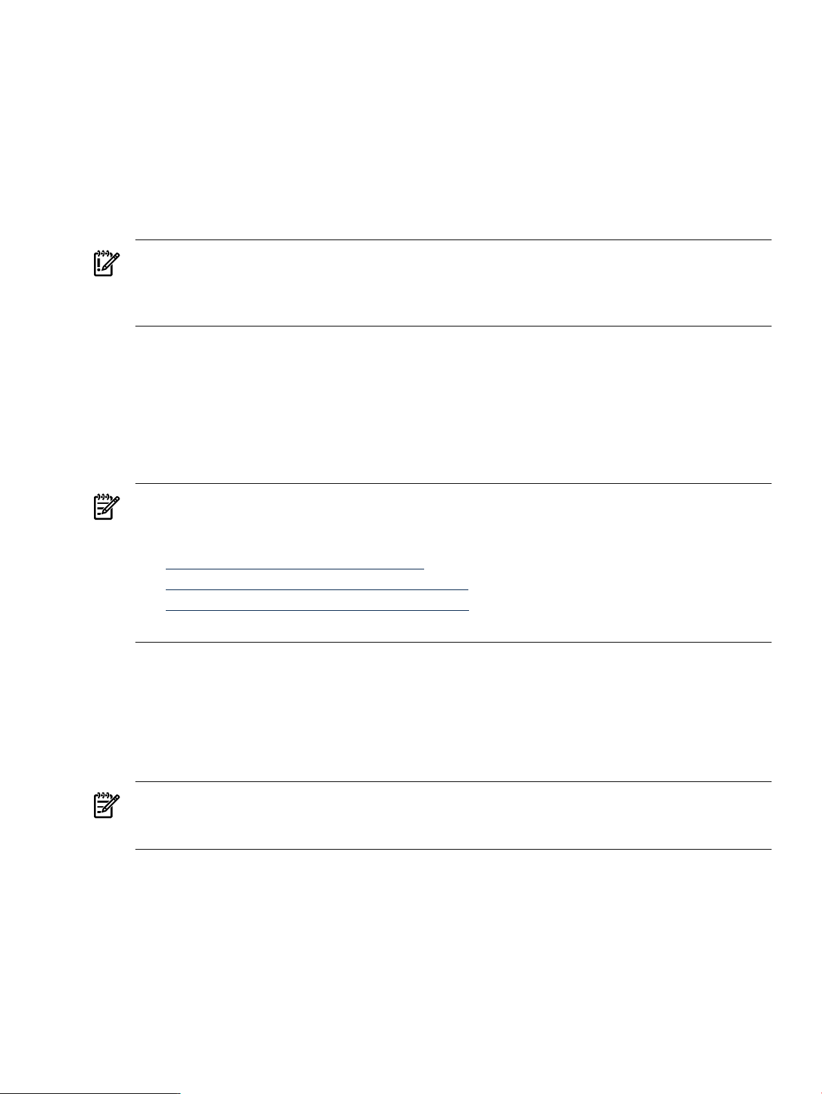
JVM Options Usage Examples

Here are some examples of JVM agent option usage:

$ -agentlib:jmeter=noalloc,appserver_port=7001,public,include=weblogic:com.bea
$ -agentlib:jmeter=nohotspots,owner_private,verbose:file=bcifilters.txt
$ -agentlib:jmeter=version
$ -agentlib:jmeter

Security Awareness

Securing Communication Between the HPjmeter Node Agent and the Console

IMPORTANT: The data stream between the HPjmeter console and agents is not protected from
tampering by a network attacker. You can help ensure that the data you view in HPjmeter
visualizers is an accurate reflection of your application's operation and that data confidentiality
is protected where needed.

Ensuring the Integrity of HPjmeter Console/Node Agent Data Transfer

For key applications in production, you may want increase your confidence that the data has
not been tampered with en route between the agents and console before you take action based
on HPjmeter metrics. Where you deem it necessary, confirm that the HPjmeter data looks
reasonable according to the usual behavior of your application. You can also pursue using secure
socket layer (SSL) tunneling to protect the integrity of data packets and to enhance the reliability
of the data reaching the HPjmeter console.

Want to Know More About Secure Socket Layer Tunneling?:

HP-UX IPSec and HP-UX Secure Shell are two HP products that provide secure socket layer
tunneling. To learn more:

• HP-UX IPSec technical documentation

• HP-UX Secure Shell overview and download

• HP-UX Secure Shell technical documentation

See also Connecting to the HPjmeter Node Agent (page 197).

Protecting Data Confidentiality During HPjmeter Console/Node Agent Communication

Data sent to the console is not encrypted by HPjmeter. If you are concerned about confidentiality
of this data, you can protect confidentiality by using SSL tunneling to encrypt the header and
data portion of each packet during transfer.

Working with Firewalls

NOTE: The console first attempts to use a port between 9505 and 9515 when arranging a port
for its server socket. If it is unable to successfully use a port from this range, it will use an ephemeral

port number.

The node agent has an open socket. Any HPjmeter console on any machine on the network (that
is not blocked by a firewall) can communicate with this node agent. If you want to have a console
contact a node agent through a firewall, you must provide a tunneling port so that the console
can contact the node agent.

Security Awareness 21

IMPORTANT: If youchoose to open a port through a firewall to enable communication between
a node agent and a console, secure the tunneling port using HP-UX Secure Shell or HP-UX IPSec.

Configuring User Access

The node agent must be started by either the same user or group as the running JVM
(recommended) or root to establish contact.

IMPORTANT: Setting access for owner or group should not be considered a security solution
because node agent to JVM communications are not secured by default—see below.

Securing Communication Between the JVM and the HPjmeter Node Agent

IMPORTANT: The data stream between the JVM and the node agent is not protected from
tampering by a user loggedinto the system runningthe JVM. For keyapplications in production,
you may want to increase your confidence that the data has not been tampered with en route
between the JVM and agent before you take action based on HPjmeter metrics.

Where you deem it necessary, either secure the communication mechanism between the JVM
and node agent (HP-UX 11i v2 or later only), or confirm that the HPjmeter data looks reasonable
according to the usual behavior of your application by independently validating its output.

To secure the communication mechanism between the JVM and node agent on HP-UX 11i v2 or
later operating systems, set the umask of the JVM process to 77 (no access except for the owner)
by executing the command

% umask 77

before running the JVM.

Related Topics

• Managing Node Agents On HP-UX (page 37)

• Node Agent Access Restrictions (page 38)

• Connecting to the HPjmeter Node Agent (page 197)

22 Completing Installation of HPjmeter

3 Getting Started

Are You Monitoring an Application or Analyzing Collected Data?

HPjmeter helps you to monitor a live run of your application. You can also view saved data
captured using HPjmeter during a live session, by using profiling or garbage collection options
when you start your application, or if you are running HP JDK/JRE 5.0.04 (or higher), by starting
and stopping profiling data collection from the command line.

Choose the get started information appropriate for your activity:

• Using HPjmeter to Monitor Applications (page 23)

• Using HPjmeter to Analyze Profiling Data (page 29)

• Using HPjmeter to Analyze Garbage Collection Data (page 31)

• Profiling with Zero Preparation (page 62)

Need a jumpstart?:

To aid in starting your use of HPjmeter, the console can display a beginning console guide
containing hints for getting started. The guide provides hints according to data set selected in
the console main pane.

To enable or disable the console guide, click Edit→ Window Preferences and toggle to the
desired option.

Using HPjmeter to Monitor Applications

The following sections summarize how to use HPjmeter to monitor applications. Detailed
descriptions of the behavior of HPjmeter are linked to from each section.

Configure and Start Your Application

1. Set the command line of your Java application to use the JVM agent and any desired agent
options.

2. Start your application with the JVM agent.

For details, see:

• Configuring your Application to Use HPjmeter Command Line Options (page 15)

• JVM Agent Options (page 17)

Confirm that the Node Agent is Running

With a standard installation, the node agent should be running on the systems where it was
installed.

For details about the node agent, see:

• Managing Node Agents On HP-UX (page 37)

Start the Console

Start the console from a local installation on your client workstation.

For starting instructions by platform, see Starting the Console.

Connect to the Node Agent from the Console

Procedure 3-2 Connection to Server (Default Mode)

To connect to a node agent:

Are You Monitoring an Application or Analyzing Collected Data? 23

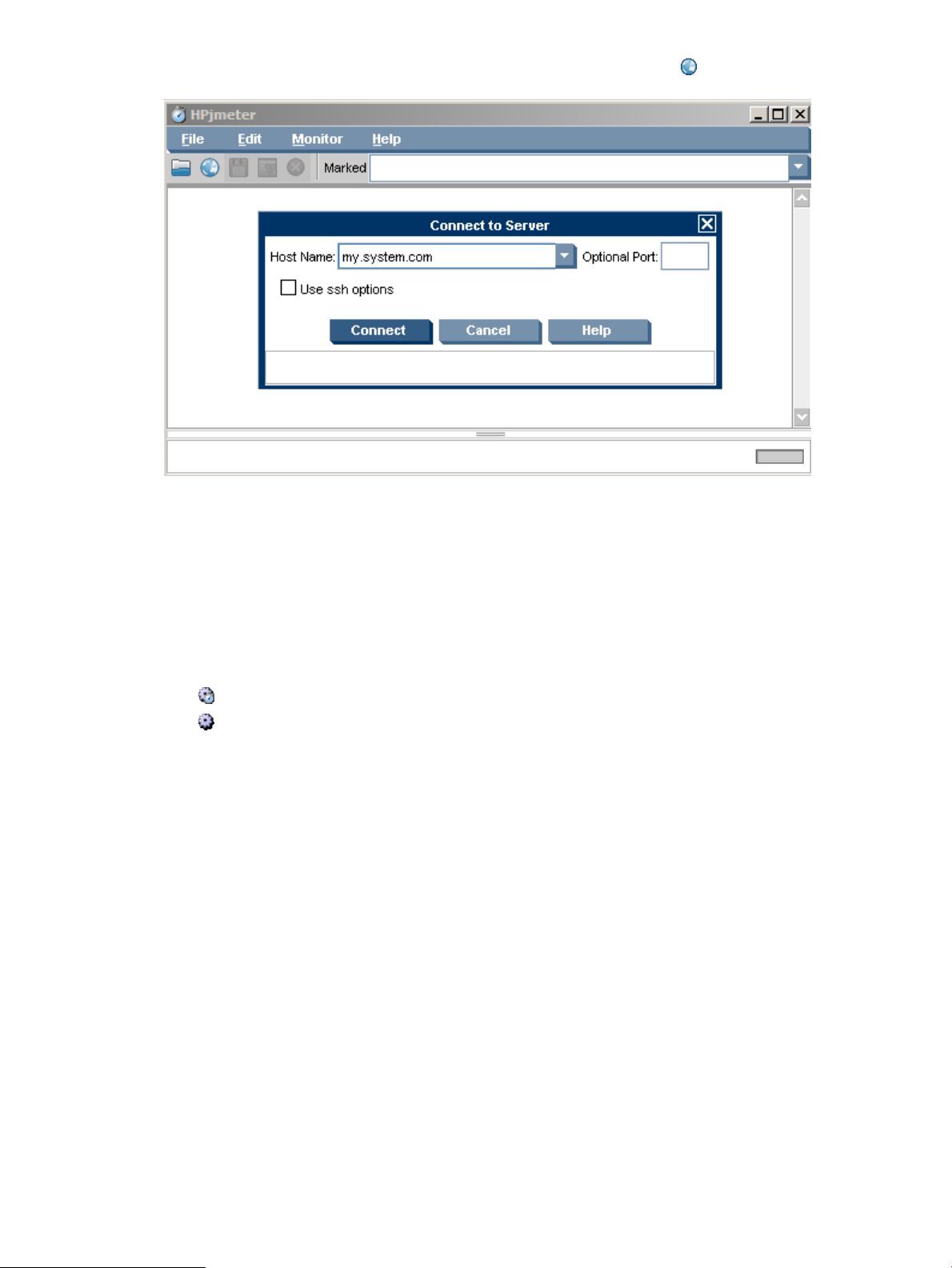
1. Choose Connect from the File menu or click Connect to server [ ]

2. In the Connect to Server dialog box, type the complete host name (server.domain.com)
on which a Java application and a corresponding node agent are running.

3. Optionally, in the Optional Port box, specify the same port number that was used when the
node agent was started.

4. Click Connect.

After a few moments, the running JVM for each application identified should appear in the
console main window pane marked with one of the following symbols:

• — A JVM that has already loaded an HPjmeter JVM agent

• — A JVM that has not yet loaded an HPjmeter JVM agent

5. Repeat the previous steps if you want to connect to several node agents on several servers
at once.

Procedure 3-3 Secured Connection to Server

To connect to a node agent via a SecureShell (SSH) tunnel:

24 Getting Started

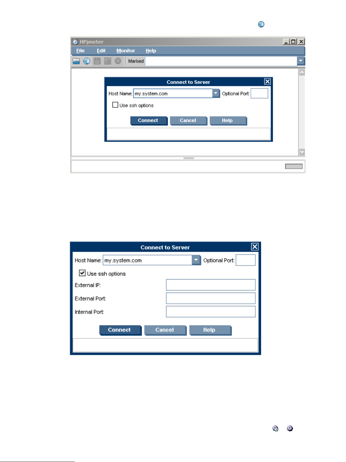
1. Choose Connect from the File Menu or click Connect to server [ ]

2. In the Connect to Server dialog box,type the complete host name (server.domain.com)

of the system that is the designated host for the SSH tunnel (the SSH delegate machine).

3. Optionally, in the Optional Port box, specify a port number through which information can

pass from the SSH delegate to the node agent.

4. Check the box labeled Use SSH Options.

The Connect to Server dialog expands to reveal required SSH attributes.

5. Type the IP address External IP) of the SSH delegate.

6. Type the port number (External Port) on the SSH delegate through which information can
pass from the SSH delegate machine to the console.

7. Type the port number (Internal Port) listened to on the console side that can accept
information from the SSH delegate machine.

8. Click Connect.

After a few moments, the running JVM for each application identified should appear in the
console main window pane marked with one of the following symbols: or .

Using HPjmeter to Monitor Applications 25

9. Repeat the previous steps if you want to connect to several node agents.

Set Session Preferences

1. Double-click on the JVM icon in the data pane for the application that you want to monitor.

This opens the Session Preferences dialog box.

26 Getting Started

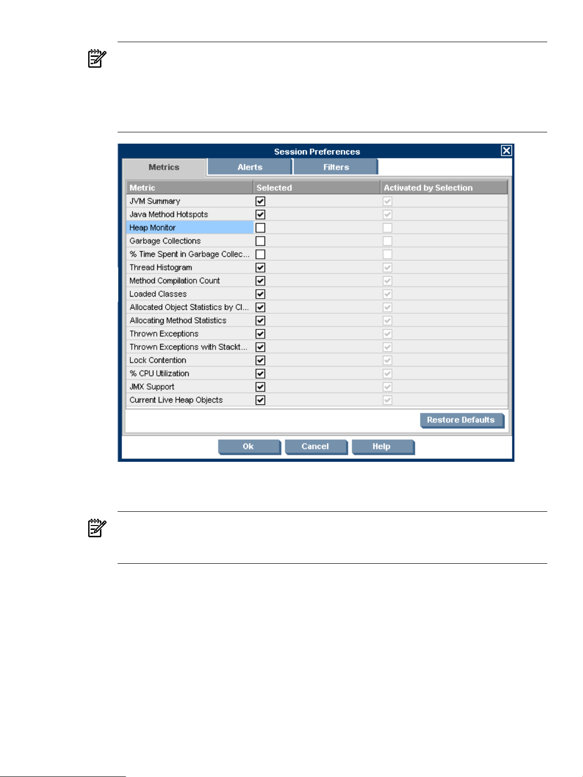
NOTE:

When the Optional Port Box Is Not Used

The console automatically attempts to use a port on the remote system between 9505 and
9515 when arranging a port for its server socket. If it is unable to successfully use a port
from this range, it will use an ephemeral port number.

2. By clicking the tabs in this dialog, you can see the default settings for metrics, filters, and
alerts. Enable or disable the settings as desired.

Interdependencies Exist Among Some Metrics and Between Some Metrics and Alerts:

Some metrics are obtained together and do not display independently from one another.
When this occurs, checking one metric may activate others, as shown in the following image.

Using HPjmeter to Monitor Applications 27

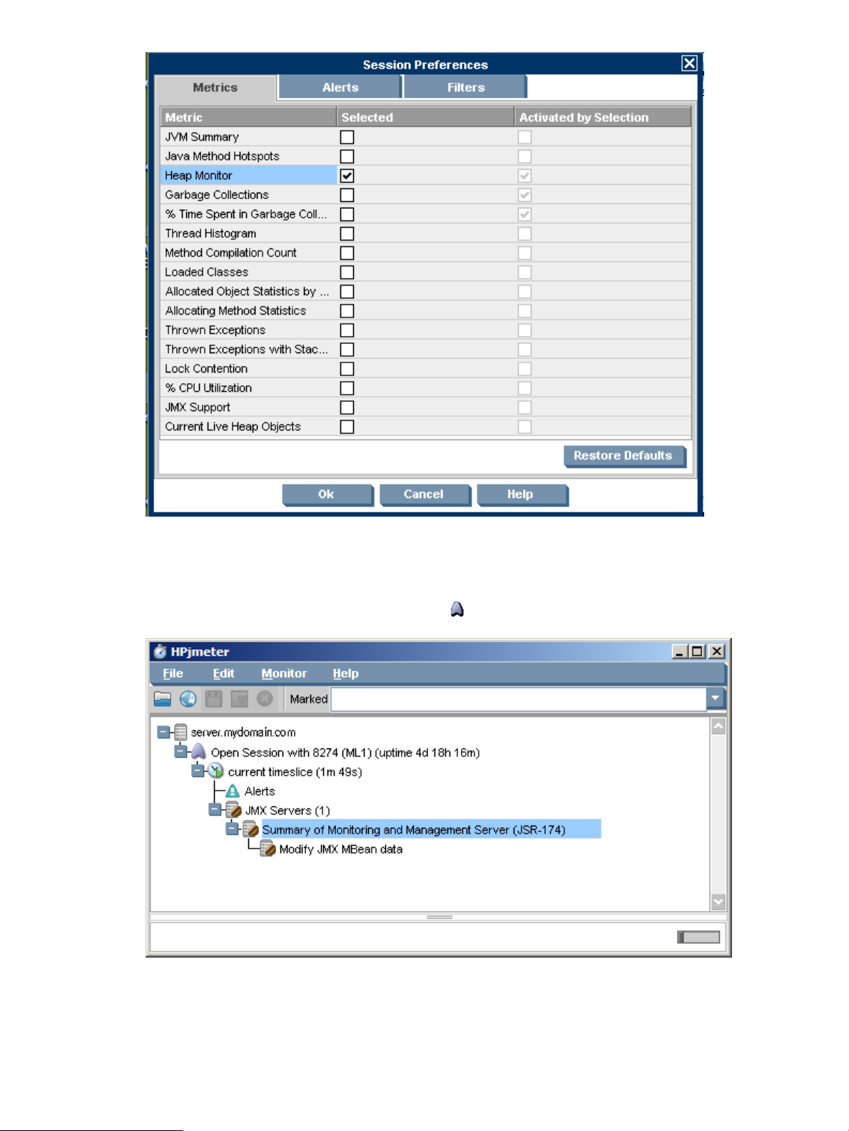
Some alerts require collection of specific metrics such that even if a metric is de-selected, it
may be activated by selection of a related alert.

3. Once all selections are made, click OK. The preferences window will close and the new Open
Session will be visible, marked by this icon:

Though it is possible to begin viewing application activity immediately in the monitoring
visualizers, you may want to wait for a short period of time before viewing some of the
metrics. The length of time needed to collect sufficient data depends on the application size,
the load imposed on the application, and on the selected preferences. Typically, a wait of 5
to 30 minutes provides sufficient data to begin seeing significant clues to the application

28 Getting Started

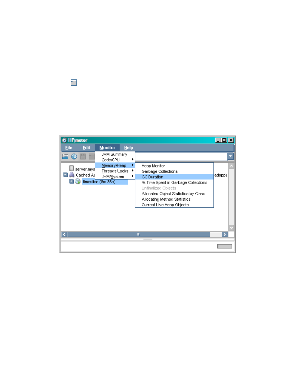
behavior and performance. A longer collection time gives you greater accuracy in the results.
For details, see: Setting Monitoring Session Preferences (page 100) .

Changing Session Preferences During a Session

With HPjmeter 4.0 and later, it is possible to change session preferences during a session.

1. Double-click the “Open Session” line in the console for the session that you want to change.

The Session Preferences window opens.

2. Alternately, selecting the “Open Session” line on the console enables the Session Preferences

icon on the console tool bar. Click the icon to open the Session Preferences window.

View Monitoring Metrics During Your Open Session

1. Click on the open session or time slice to highlight the data that you would like to view.

2. Use the Monitor menu on the console main window to select the metrics that you want to

see. Mousing over each category in the cascading menu will reveal the relevant metrics for
that category.

3. Click a metric to open a metric visualizer displaying the chosen data.

For details on individual metrics and how to interpret the data display, see:

• Using Monitoring Displays (page 117)

• Monitoring Applications (page 36)

See also:

• Saving Monitoring Metrics Information (page 38)

• Using Visualizer Functions (page 116)

Using HPjmeter to Analyze Profiling Data

The following steps summarize how to use HPjmeter to view profiling information from your
applications.

Using HPjmeter to Analyze Profiling Data 29

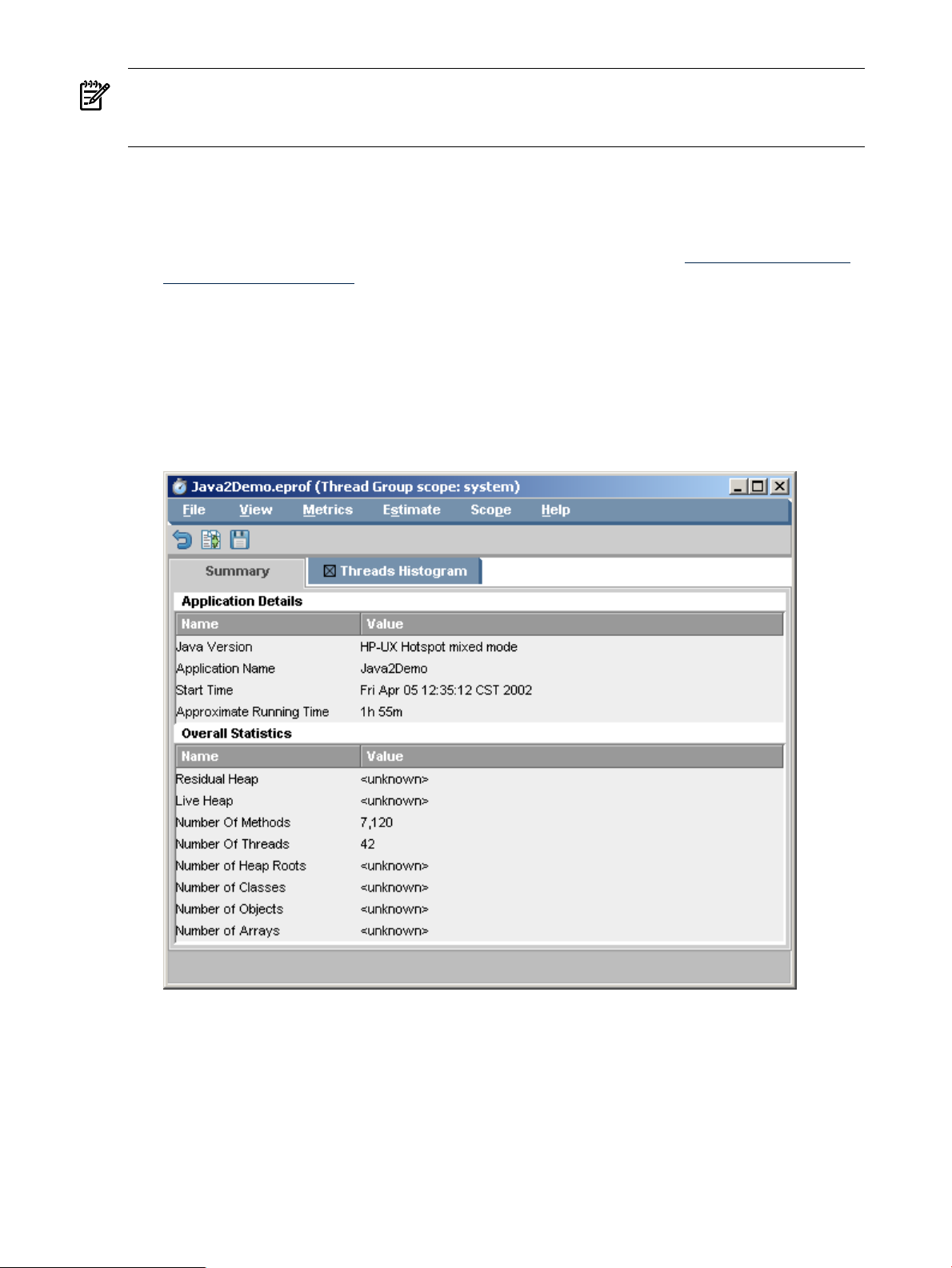
NOTE: If you are running the HP JDK/JRE 5.0.04 or later, you can send a signal to the running
JVM to start and stop a profiling data collection period with zero preparation and no interruption
of your application. See Profiling with Zero Preparation (page 62).

1. Configure your application.

Change the command line of your Java application to collect the desired type of data: -Xeprof
to collect execution profiling information, -agentlib:hprof to generate heap dump at program
exit, or -XX:+HeapDump to enable generation of heap dumps using the SIGQUIT signal.
There are additional heap dump options. For more details, see the Java™ Troubleshooting

Guide for HP-UX Systems .

2. Run the application to create a data file.

3. Start the console from a local installation on your client workstation.

4. Click File→Open File to browse for and open the data file, or drag and drop the file onto
the console.

5. For all profiling data types, a viewer window opens and displays a set of tabs containing
summary and graphical metric data. You will also see the Metrics and Estimate menus
containing additional metric display choices, and a control menu for changingthread scope.

30 Getting Started

6. Click among the tabs to view available metrics.

Use the Metrics or Estimate menus to select additional metrics to view. Each metric that
you select opens in a new tab. Mousing over each category in the cascading menu will reveal
the relevant metrics for that category.

For details on individual metrics and how to interpret the data display, see:

• Collecting Profile Data (page 61)

• –Xeprof and –agentlib:hprof Profiling Options and Their Corresponding Metrics (page 65)

• Profiling Applications (page 58)

• Using Profile Displays (page 137)

• Using Visualizer Functions (page 116)

Using HPjmeter to Analyze Garbage Collection Data

The following steps summarize how to use HPjmeter to view garbage collection information
from your applications.

NOTE: If you are running the HP JDK/JRE 5.0.14 or 6.0.02 version, you can send a signal to the
running JVM to start and stop a verbose GC data collection period with zero preparation and no
interruption of your application. See Collecting GC Data with Zero Preparation (page 83).

1. Configure your application.

Change thecommand line of yourJava application to use -Xverbosegc or -Xloggc options
to capture garbage collection data.

2. Run the application to create a data file.

3. Start the console from a local installation on your client workstation.

Using HPjmeter to Analyze Garbage Collection Data 31

4. Click File→Open File to browse for and open the data file, or drag and drop the file onto
the console.

5. A GC viewer window opens and displays a set of tabs containing summary and graphical
metric data.

6. Click among the tabs to view available metrics.

For details on individual metrics and how to interpret the data display, see:

• Analyzing Garbage Collection Data (page 80)

• -Xverbosegc and -Xloggc Options and Their Corresponding Metrics (page 85)

• Using Specialized Garbage Collection Displays (page 157)

• Using Visualizer Functions (page 116)

Monitoring Demonstration Instructions

HPjmeter includes two sample applications that you can run to see live examples of a “memory

leak” and a thread deadlock situation. You will be able to use the visualizers to examine data

during the demonstration session.

Here are the general steps for running the sample applications.

1. Start the console.

2. Start the node agent if it is not running as a daemon.

3. Start the sample application from the command line:

$ cd $JMETER_HOME/demo
$ export LD_LIBRARY_PATH=$JMETER_HOME/lib/$ARCH
$ java -agentlib:jmeter -jar ML1.jar

As a convenience, HPjmeter includes a script that sets up the library path and
bootclasspath using a JVM found at installation time. To use this script, type:

32 Getting Started

$ cd $JMETER_HOME/demo
$ ../bin/run_simple_jvmagent -jar sample_program

Use the file name of the specific sample you want to run in place of sample_program.

4. In the console main window, click Connect and type in the host name of the machine that
runs the sample application. If you specified a port number when starting the node agent,
use the same port number. Otherwise, leave the port number box empty.

5. An icon representing the host appears in the main window. After a few moments, the console
also shows the sample application as a child node of the host.

6. Double-click the application node to open a monitoring session with the application.

The dialog box for setting session preferences will open.

7. Click OK to accept the default settings for metrics, filters and alerts.

The console main window now displays the open session.

Memory Leak Applications

There are two sample applications ML1 and Pi, that demonstrate how memory leak alerts work
in HPjmeter. ML1 demonstrates how Java Collection Leak alerts work, and Pi demonstrates how
how Array Leak alerts work.

The ML1 example uses a simple Java program that allocates some objects, and uses a
java.util.Vector object to retain references to some of the objects,thus exhibiting the behavior
of a memory-leaking application.

This application is configured to leak memory at the rate of about 10 MB per hour. The demo
application is available from the HPjmeter installation directory:

Source: $JMETER_HOME/demo/ML1.java

Binary: $JMETER_HOME/demo/ML1.jar

Use —jar ML1.jar with the run_simple_jvmagent script to start the sample.

When measuring the sample applications, allow considerable time for the heap to mature and
stabilize, and for the JVM agent to collect memory leak data. Eventually, you will see two alerts:

• Expected Out Of Memory Error Alert (page 110) with the leaking rate.

• Java Collection Leak Locations Alert (page 111) with the leak location.

When using the default garbage collectors and heap size for Java HotSpot Virtual Machine 1.4.2,
the detection of a memory leak for this demonstration program occurs after about 20 minutes.
This time can be substantially longer when using a different JVM or non-standard garbage
collector or heap settings.

In real situations, the detection time depends on the maximum heap size, the size of the leak,
the application running time, and the application and load characteristics. Typically, the detection
will occur in about one hour.

Here is a Java collection leak alert for the sample program:

Here is the heap display for the sample program:

Monitoring Demonstration Instructions 33

Figure 3-1 Heap Display Showing Possible Memory Leak Behavior

See also Heap Usage Notification (page 111).

The Pi sample program uses a simple Java program that allocates some arrays, thereby exhibiting
the behavior of a memory-leaking application. The demo application is available from the
HPjmeter installation directory:

Source: $JMETER_HOME/demo/Pi.java
Binary: $JMETER_HOME/demo/Pi.jar

Use -jar Pi.jar with the run_simple_jvmagent script tostart the sample. When measuring
the sample application, allow considerable time for the heap to mature and stabilize, and for the
JVM agent to collect memory leak data. Eventually, you will see two alerts:

• Expected Out Of Memory Error Alert (page 110) with the leaking rate.

• Array Leak Locations Alert (page 112) with the leak location.

When the default garbage collectors and heap size for Java HotSpot Virtual Machine 1.5.0.07 are
used, the detection of a memory leak for this demonstration program occurs after about 90
minutes. This time can be substantially longer when using a different JVM or nonstandard
garbage collector or heap settings.

In real situations, the detection time depends on the maximum heap size, the size of the leak,
the application running time, and the application and load characteristics. Typically, the detection
will occur in about two hours.

Here is an Array Leak alert for the sample program:

Thread Deadlock Sample

This sample application demonstrates how HPjmeter detects deadlocked threads.

34 Getting Started

The example creates pairs of threads every 30 seconds, stopping at 50 threads, which synchronize
work using shared locks. Occasionally, the program reverses the order in which locks are taken,
eventually causing a deadlock, which generates a Thread Deadlock Alert (page 115).

The demo application is available from the HPjmeter installation directory:

Source: $JMETER_HOME/demo/DL1.java

Binary: $JMETER_HOME/demo/DL1.jar

Use —jar DL1.jar with the run_simple_jvmagent script to start the sample.

Use the Thread Histogram display to see the thread activity. Deadlocked threads show a solid
red bar.

Figure 3-2 Thread Deadlock Example Display

Monitoring Demonstration Instructions 35

4 Monitoring Applications

In addition to using HPjmeter when you notice a problem, you can also use it to prevent problems.
For example:

• You can use HPjmeter to check the efficiency of your applications, even if you don't notice
a problem.

To make it easier to detect problems, you should periodically review key metrics for your
application to establish a baseline profile.

To save metrics information to a file that you can review later, see Saving Monitoring Metrics

Information (page 38).

• You can check your application after making code or configuration changes to see how
performance might have been affected.

NOTE: You cannot use HPjmeter to monitor Java applets in a production environment.

Controlling Data Collection and Display

HPjmeter provides two methods to control how information is collected and displayed.

JVM agent filters. The include and exclude options to the JVM agent allow you to filter

metrics by class name.

JVM agent filters are configured when you start the JVM, and cannot be dynamically changed.

Console filters are configured when you open a session with a JVM agent, and can be changed

from session to session. With HPjmeter 4.0 and later, these filters can also be changed during a
session.

NOTE: In metrics displays, you can see the list of filters in effect while the data was collected,

including default agent filters, by clicking the icon.

Related Topics

• Setting filters with JVM Agent Options (page 17)

• Setting filters by Setting Monitoring Session Preferences (page 100)

Setting Data Collection Preferences

HPjmeter allows you to control how metrics are collected to give you control over the amount
of detail and possible performance impact on your application.

When you open a session between the console and JVM agent, theSession Preferences window
lets you select from the available metrics, filters, and alerts.

When you open a session to monitor your applications, you can:

• Specify which metrics to collect.

• Enable alerts to give notifications when specific conditions occur.

• Specify filters to include or exclude specific classes.

Related Topics

• Controlling Data Collection and Display (page 36)

• Performance Overhead on Running Applications (page 187)

• Specifying Metrics to Collect for Monitoring (page 100)

36 Monitoring Applications

Managing Node Agents

Each managed node requires an HPjmeter node agent that manages communication between
the console and JVM agents.

Once the Session Preferences window closes, and after waiting for a few moments, you should
see the running JVM agents listed below the connected server host name. If no JVM appears,
check that a node agent is running on that server. If no node agent is running, the console cannot
show the JVM agents.

On HP-UX, you can run the node agent as a daemon or service for automatic, continuous
operation, or as a manual process when you do not need continuous operation.

Managing Node Agents On HP-UX

Running Node Agent as a Daemon

When you install HPjmeter on HP-UX systems, you can start the node agent as a daemon for
continuous automatic operation.

NOTE: Though you can run the node agent continuously, the node agent is not a high availability
application.

As a daemon, the node agent can use an alternate port number. To specify a different port number,
edit the /sbin/init.d/HPjmeter_NodeAgent file, add the -port option, and manually
start the node agent.

To start or stop the node agent daemon on HP-UX PA and IA:

$ /sbin/init.d/HPjmeter_NodeAgent start|stop

To change default options, such as port number, edit the contents of the file.

Verifying HP-UX Daemon is Running

When the node agent is running as a daemon on a HP-UX system, use these steps to verify that
the node agent is running:

1. You must be logged in with root permissions.

2. Check that these files exist:

• /sbin/init.d/HPjmeter_NodeAgent

• /sbin/rc3.d/S999HPjmeter_NodeAgent

3. Use the ps command, or its equivalent on your system:

$ ps -ef | grep node

The result should show:

$ JMETER_HOME/bin/nodeagent -daemon

where

JMETER_HOME=/opt/hpjmeter

The –daemon flag indicates that the node agent is running as a daemon.

To start or stop the node agent daemon manually:

$ /sbin/init.d/HPjmeter_NodeAgent start|stop

Starting Node Agents Manually

If you cannot use the node agent daemon or you need to set up access restrictions, you can start
a node agent manually. For information about access restrictions, see Working with Firewalls

(page 21).

A node agent must be running before the console can connect to a managed node to discover
your applications and open monitoring sessions.

Managing Node Agents 37

Start the node agent from the command line by typing:

$ JMETER_HOME/bin/nodeagent

where $JMETER_HOME has the default value of

JMETER_HOME=/opt/hpjmeter

You can run the node agent as a background process. By default, the node agent listens for
console connections on port 9505, but you can designate an alternate port number using this
option: -port port_number

Related Topics

• Working with Firewalls (page 21)

• Running Node Agent as a Daemon (page 37)

Stopping Node Agents

To stop a manually started node agent, abort the process.

Node Agent Access Restrictions

To make the JVM agent visible to the corresponding node agent, start a node agent with the same
group ID or user ID of each JVM process whose JVM agent uses the group_private (default)
or owner_private options. Node agents started as root will see all JVM agents regardless of
the ownership ID used on the JVM agent.

Running Multiple Node Agents

To run multiple node agents on the same managed node, each node agent must listen on a
different port to control visibility to JVMs. Use the node agent port option to specify a port
number. Each user or group must remember the port on which their node agent is running to
connect to it.

To provide more secure access, run multiple node agents and use the owner_private or
group_private option for the JVM agent. For more information, refer to Node Agent Access

Restrictions (page 38).

Saving Monitoring Metrics Information

HPjmeter offers two methods to save monitoring metrics information to a file.

• If you know in advance that you want to capture information for an entire application
session, you can run the JVM agent monitor_batch option when you start the application.
See JVM agent option monitor_batch[:file=filename].

When you save information using the monitor_batch option, the information is captured
from the start of the application session in a file on the managed node. To stop capturing
information, stop your application. For more information, see

monitor_batch[:file=filename].

• If you want to capture information from the start of the console session to the current time,
click File→Save as to name the saved data file. For details, see Saving Data from the Console

(page 39)

Each of these methods saves metrics information that you can later load into the console using
the Open File button or menu option., or dragging and dropping the file onto the console.

You can use these data files to capture information from live sessions to review later or to send
to a development team to show the state of your application.

38 Monitoring Applications

NOTE: Saved data files can be quite large. If you expect to keep the files or you plan to transfer
the files, compress the files for speedier transfer.

Compressing the files also reduces the chances that the file could be corrupted during a transfer.
You can compress various profile data files; for example: .vgc, .hprof (ascii text and binary
format), .eprof, and .hpjmeter. The preferred compression format is gzip. HPjmeter 4.1 and
higher can read gzip compressed files, without having to expand them.

Saving Data from the Console

When you save information using the Save as button from the console, the information from
the start of the console session is saved in a file on the system running the console.

In addition, you can save information from any cached session available on the console.

To save information as a console snapshot:

1. Go to the console main window.

2. Select a live or cached session node from the data tree.

3. Click File→Save as from the main window tool bar.

This opens the file chooser that allows you to specify where to save the file.

4. In the file chooser, select the directory in which you want to save the snapshot file.

5. Specify the snapshot file name.

The file chooser automatically appends the extension .hpjmeter to your file name.

To prevent adding the file name extension, use double quotes to surround the file name.

6. Click Save.

HPjmeter writes the session information to the file.

NOTE: When you close the console, HPjmeter checks for session data that has not yet been
saved. You are given an opportunity to save collected data, but you can choose not to do so.

If you typically do not save monitoring session data, you can turn this checking function off by
selecting Edit→Window Preferences and unchecking Confirm save when closing the main
window.

Naming Monitoring Data Files

When you save monitoring data, HPjmeter appends the suffix .hpjmeter at the end of the file
name by default. You may want to follow this convention when naming data files saved during
a monitoring session, but it is not required.

Diagnosing Errors When Monitoring Running Applications

Issues or symptoms you might notice and how to identify problems and remedy them.

Identifying Unexpected CPU Usage by Method

To identify methods with unexpected CPU usage, use the Java Method HotSpots display.

This metric may require a relatively long time to stabilize, and is tuned for large, multi-CPU
systems.

To determine if the CPU usage is unexpected, you need to know and understand how the
application works.

If this metric shows a large percentage of CPU time spent in just a few methods listed at the top,
it indicates that a performance problem may exist or there is room for improvement.

Naming Monitoring Data Files 39

Typically, when the top entry is represented by a single-digit percentage, you should not see
application CPU performance issues unless the entry describes an obscure method that you did
not expect to see.

Related Topics

• Java Method HotSpots (page 118)

• Process CPU Usage Alert (page 113)

• System CPU Usage Alert (page 114)

Viewing the Application Load

Use the Heap Monitor display.

This metric shows how busy the application is. It checks to see whether it is doing lots of
allocations, which typically corresponds to the load level, or whether it is idle.

When you select a coarse granularity of the view (1 to 24 hours), and assuming that there is no
memory leak, you will notice the overall change of behavior in heap size and garbage collection
pattern. This setting can help you understand the correlation between the application load and
the pressure on the heap.

If it seems a significant amount of time is spent in garbage collection, (gray in selected areas of
the display), it means that the heap was not adequately sized — it was too small for the load on
the application at that time. This behavior may also mean that the load was too high for the given
hardware and software configuration.

Related Topics

• Heap Monitor (page 122)

• Percentage of Time Spent in Garbage Collection (page 125)

• Heap Usage Notification (page 111)

Checking for Long Garbage Collection Pauses

Use the Heap Monitor display and select the shortest time interval.

Most garbage collections take several seconds at most to execute. Very large heaps, however,
may take up to several minutes.

Although the display does not show numerical values for the garbage collection duration, you
can look for extra wide garbage collection bars, which correspond to garbage collection pauses.
They will likely cause transient service-level objective (SLO) violations.

If intermittent, very long garbage collections are a potential problem in a given environment,
you can select appropriate garbage collection algorithms with a JVM option. Refer to your JVM
documentation.

Related Topics

• Heap Monitor (page 122)

• GC Duration (page 124) and GC Duration Notification (page 110)

• Garbage Collections (page 123)

• Heap Usage Notification (page 111)

• Data Collection with -Xverbosegc (page 80)

• Basic Garbage Collection Concepts (page 87)

Checking for Application Paging Problems

Use the Heap Monitor display, selecting a short time interval.

If multiple consecutive garbage collections take extraordinary time to run, this may indicate an
excessive paging problem, called thrashing, where the physical memory available to the
application is too small for the specified maximum size.

40 Monitoring Applications

You can verify this using a system tool like HP GlancePlus. The possible remedies for thrashing:

• Decrease the maximum heap size, which corresponds to a decrease of the maximum load
supported by the application.

• Eliminate other load on the system.

• Install more physical memory.

Related Topics

• Heap Monitor (page 122)

• Garbage Collections (page 123)

• Heap Usage Notification (page 111)

Identifying Excessive Calls to System.gc()

Use the Heap Monitor display.

When a high level of detail is selected (1 to 20 minutes), this metric can help detect if calls to
System.gc() are creating a performance problem. When your application calls this method,
you see that the heap size does not go to the local maximum before a garbage collection happens.
However, from time to time, the JVM may automatically invoke garbage collection in such
circumstance, too.

A rule of thumb is that if over half of all garbage collections seem to happen when the heap is
not full, then it may mean explicit calls to System.gc() are occurring. Remove explicit calls
from your application, either by modifying the code or by using an appropriate JVM option.
These calls rarely improve the overall performance of the application.

Related Topics

• Heap Monitor (page 122)

• Garbage Collections (page 123)

• Heap Usage Notification (page 111)

• Using Specialized Garbage Collection Displays (page 157)

Reviewing the Percentage of Time Spent in Garbage Collection

The percentage of time your application spends in garbage collection can help you identify
potential problems. Use the % Time Spent in Garbage Collection display to view this
information. For details, see Percentage of Time Spent in Garbage Collection (page 125).

In this example, you see a fairly normal application behavior.

• A low flat graph

• A low average value, represented by the red line

Diagnosing Errors When Monitoring Running Applications 41

Figure 4-1 Example Metric: Percentage of Time Spent in Garbage Collection When Application
Behavior is Normal

This next example shows an application with a potential memory leak.

• A rising trend in the percentage of time spent in garbage collection.

Figure 4-2 Example Metric: Percentage of Time Spent in Garbage Collection When Application
Shows Potential Memory Leak

Related Topics

• How Memory Leak Detection Works (page 189)

• Expected Out Of Memory Error Alert (page 110)

• Java Collection Leak Locations Alert (page 111)

42 Monitoring Applications

• Array Leak Locations Alert (page 112)

• Class Loaders (page 150)

Checking for Proper Heap Sizing

Efficiencies inprogram performance can be obtained by allocating the optimal amount of memory
for the heap according tothe needs of the program and the operation of the JVM garbage collection
routine. Checkingactivity in the heap and comparing to garbagecollection frequency and duration
can help you determine optimal heap size needed for best performance from your application.

See the following sections for metrics that give insight into these aspects of the system:

• Current Live Heap Objects (page 129)

• Heap Monitor (page 122)

• Garbage Collections (page 123)

• Heap Usage Notification (page 111)

For detailed GC analysis, run your application with -Xverbosegc and use the HPjmeter GC
viewer to analyze GC activity in the heap. For additional details on memory usage, run your
application with -agentlib:hprof.

Confirming Java Memory Leaks

HPjmeter can automatically detect Java memory leaks, alerting you about the issue before the
application crashes.

After running for some time, Java applications can terminate with an out-of-memory error, even
if they initially had an adequate amount of heap space. The direct cause of this error is the inability
of the garbage collector to reclaim enough heap memory to continue.

The root cause of this problem is that some objects, due to the design or to coding errors, remain
live. Such objects, called lingering objects, tend to accumulate over time, clogging the heap and
causing multipleperformance problems, and eventually leading to theapplication crash. Although
the nature of this phenomenon is different than memory leaks in C/C++, Java lingering objects
are also commonly called memory leaks.

A more subtle problem that can cause an out-of-memory error occurs when the Permanent
Generation area of memory becomes full of loaded classes. Running -agentlib:hprof can
provide class loading data that can help to reveal whether this problem is occurring.

Related Topics

• Expected Out Of Memory Error Alert (page 110)

• Garbage Collections (page 123)

• Current Live Heap Objects (page 129)

• How Memory Leak Detection Works (page 189)

• Java Collection Leak Locations Alert (page 111)

• Array Leak Locations Alert (page 112)

• Loaded Classes (page 135)

• Class Loaders (page 150)

Determining the Severity of a Memory Leak

When HPjmeter automatically reports memory leaks, use the Garbage Collections and Heap
Monitor displays to help you visualize object retention. Object retention may indicate Java

memory leak problems.

Selecting large view ports, one hour or longer, allows you to easily see the trend in the heap size
after garbage collection and its increase rate, if any. You can visually assess the danger associated
with the memory leak, and estimate, based on the knowledge of the total heap size, when the
application would run out of memory, whether it is a matter of minutes, hours, or days.

Diagnosing Errors When Monitoring Running Applications 43

The Heap Monitor and Garbage Collections data help you determine if an observed application
termination could have been caused by running out of heap space.

The Heap Monitor gives the idea about the overall heap limit, while the Garbage Collections
display shows the size of heap after each garbage collection.

If the heap size shown by Garbage Collections converges toward the heap limit, the application
will, or has, run out of memory.

Related Topics

• Expected Out Of Memory Error Alert (page 110)

• Garbage Collections (page 123)

• Heap Monitor (page 122)

• Current Live Heap Objects (page 129)

• How Memory Leak Detection Works (page 189)

• Heap Usage Notification (page 111)

• JMX Memory Tab (page 49)

Identifying Excessive Object Allocation

Use the Allocated Object Statistics by Class display.

This metric shows the most frequently allocated object types.

Verify your understanding of the application memory use pattern with this metric. Resolving
this problem requires knowledge of the application.

Related Topics

• Allocated Object Statistics by Class (page 127)

Identifying the Site of Excessive Object Allocation

Use the Allocating Method Statistics display.

This metric shows the methods that allocate the most objects. This metric is useful when you
decide to decrease heap pressure by modifying the application code.

Related Topics

• Allocating Method Statistics (page 128)

Identifying Abnormal Thread Termination

Look for the Abnormal Thread Termination Alert, which allows you to see a list of the uncaught
exceptions.

You can then use the Thread Histogram to investigate possible problems.

Terminated threads appear as a discontinued row. HPjmeter is unable to tell if the thread was
prematurely terminated or just completed normally. This is a judgment call, but in many cases
the analysis does not require extensive application knowledge.

If just one thread from a group of similar threads (by name, creation time and characteristics)
terminates, it is very likely that it was stopped.

A thread terminating abnormally does not necessarily bring the application down, but can
frequently cause the application to be unresponsive.

Related Topics

• Abnormal Thread Termination Alert (page 108)

• Thread Histogram (page 131)

Identifying Multiple Short-lived Threads

Use the Thread Histogram.

44 Monitoring Applications

Threads are relatively costly to create and dispose; usually a more efficient solution is through
thread pooling.

Related Topics

• Thread Histogram (page 131)

• Identifying Abnormal Thread Termination (page 44)

Identifying Excessive Lock Contention

Use the Thread Histogram.

There is no simple answer to how muchlock contention is excessive. A multi-threaded application
normally exhibits some lock contention. With the Thread Histogram display, you can identify
the threads that clash over the same lock by visually comparing the pattern for the lock contention
(the red area) across several threads.

In situations when a small number of threads are involved in contention, you need to compare
a red area from one thread to the red and orange area in another thread. This may help identify
the involved locks, but it requires understanding the threading of the given application.

Some applications, such as WebLogic from BEA, use basic-level synchronization for multiple
threads reading from a single socket. This typically appears as very high lock contention for the
involved threads. If there are N threads using this pattern, the average lock contention for them
will be (N-1)/N*100%. Even though this kind of lock contention seems to be harmless, it
unnecessarily stresses the underlying JVM and the operating system kernel, and usually does
not bring a positive net result. There is a WebLogic option that can fix this. See the release notes
for your version of WebLogic for details.

You may attempt to decrease the level of lock contention by decreasing the number of involved
threads. If this does not help, or if it decreases the application throughput, you should deploy
the application as a cluster. At the same time, large servers, for example 8-way, can be
re-partitioned as a group of smaller virtual servers.

If the lock contention appears in your application, rather than a third-party application, you may
be able to change your code to use different algorithms or to use different data grouping.

Related Topics

• Lock Contention (page 133)

• Thread Deadlock Alert (page 115)

• Thread Histogram (page 131)

Identifying Deadlocked Threads

HPjmeter allows you to enable an alert that identifies deadlocked threads. You can then use the
Thread Histogram to get more specific information.

Deadlocked threads represent a multi-threaded program error.

Thread deadlock is the most common cause of application unresponsiveness. Even if the
application is still responding, expect SLO violations.

Restart the application that experienced the deadlock, and fix the application code to avoid future
deadlocks.

Related Topics

• Thread Deadlock Alert (page 115)

• Thread Histogram (page 131)

Identifying Excessive Thread Creation

Use the Thread Histogram to identify excessive thread creation.

Diagnosing Errors When Monitoring Running Applications 45

The Thread Histogram shows the number of threads existing in the observed period of time. By
selecting the smallest time interval, one minute, you can see an estimate of the number of
simultaneously active threads. Most operating systems have a limited capacity for the number
of threads a single process may create. Exceeding this capacity may cause a crash. Although
HPjmeter cannot indicate whether or not this will happen, the intensity of the new thread creation
may suggest deeper analysis is needed in this area.

Adjusting kernel parameters may increase the threads per process limit.

Sometimes an application may exhibit threads leak, when the number of dynamically created
threads is unconstrained and grows all the time. Tuning kernel parameters is unlikely to help
in this situation.

Related Topics

• Thread Histogram (page 131)

Identifying Excessive Method Compilation

HPjmeter allows you to enable an alert that identifies excessive method compilations. You can
then use the Method Compilation Count display to view the specific method or methods that
caused the alert.

Symptoms of excessive method compilation include poor application response because the JVM
is spending time re-compiling methods.

The Method Compilation Count display shows the methods that have been compiled, sorted by
number of compilations.

Figure 4-3 Example Metric: Method Compilation Count

Excessive method compilation is rare, especially with newer releases of JVM. Sometimes, due
to a defect in the JVM, a particular method can get repeatedly compiled, and de-optimized. This
means that the execution of this method oscillates between interpreter and compiled code.
However, due to the stress on the JVM, such phenomena are typically much more costly than
just running this method exclusively in interpreted mode.

Repeated compilation problems may result in SLO violations and will affect some or all
transactions. Read the JVM Release Notes to learn how to disable compilationof selected methods
for the HP Java HotSpot Virtual Machine.

46 Monitoring Applications

Related Topics

• Excessive Compilation Alert (page 110)

• Method Compilation Count (page 134)

• Method Compilation Frequency (page 135)

Identifying Too Many Classes Loaded

Use the Loaded Classes display.

This display can be used to determine if the pool of classes loaded into memory stabilizes over
time to a constant value, which is normal.

In some JVMs, like HotSpot, loaded classes are located in a dedicated memory area, called the
Permanent Generation, which is typically much smaller that the whole heap. If the application
repeatedly loads new classes, either from external sources, or by generating them on the fly, this
area overfills and the application abnormally terminates. This will correspond with the value of
this metric constantly growing up to the point of failure.

If you find that the application terminates because the number of loaded classes is too large for
the area of memory dedicated to this purpose, you can increase the heap area for the class storage
by using a JVM option. However, if changing the dedicated memory size will not help the
situation because the number of the loaded classes is unconstrained, this is an application design
issue that needs to be solved.

NOTE: An overflow of the area dedicated to class storage can cause the application to terminate,
sometimes with an OutOfMemoryError message, even if there is plenty of space available on
the heap. Consult your JVM documentation on how to increase the area dedicated for class
storage, if necessary.

Related Topics

• Loaded Classes (page 135)

• Class Loaders (page 150)

• Expected Out Of Memory Error Alert (page 110)

Using the JMX Viewer

The JMX viewer provides access to data collected from the operation of JMX servers inside the
Java Virtual Machine for Java 1.5.x versions.

The viewer also provides you with the ability to interject in some operations of the JVM and to
manipulate the operation and attributes of MBeans that you have defined. Using HPjmeter

monitoring displays, you can observe the effect of changing the characteristics of MBeans that

you have loaded into the JMX server of the virtual machine.
Opening the JMX viewer On opening a session with an application running on Java 1.5.x, a

data node displays in the main console to represent current data collected from the JVM.

Using the JMX Viewer 47

Figure 4-4 Main Console Showing an Expanded JMX Server Node in an Open Session

To access this summary data, double-click on the summary JMX server node. The summary JMX
Viewer opens. For information on this part of the JMX Viewer, see Understanding the JMX

Summary View (page 48).

To manipulate some JVM and MBean functions on this server, expand the summary node and
double-click the entry labeled Modify JMX MBean data. The server JMX Viewer opens. For
information on this part of the JMX Viewer, see Changing Mbean Values and Monitoring the

Result (page 52)

NOTE: This functionality is available only during an open session. No record of the actions
taken within the JMX viewer are saved. To preserve a record of changes occurring in the
application run due to manipulation of the JMX server and MBeans, save the monitoring session

data for later review. Use the monitoring metric visualizers to view the saved data.

See also

• View Monitoring Metrics During Your Open Session (page 29)

• Tapping in to Standard Management of the Java Virtual Machine (page 190)

Understanding the JMX Summary View

The JMX viewer opens in the Summary view with five tabs displayed:

• JMX Summary Tab (page 48)

• JMX Memory Tab (page 49)

• JMX Threads Tab (page 51)

• JMX Runtime Tab (page 52)

• JMX Notifications Tab (page 52)

JMX Summary Tab

The Summary tab shows a collection of data about the operating system and hardware, allocated
memory, current heap usage, and class loading status. Values are updated throughout the
duration of the open session.

48 Monitoring Applications

Figure 4-5 Appearance of the Summary JMX Viewer When First Opened

JMX Memory Tab

Fluctuations in memory usage in heap and non-heap areas are graphically displayed and
periodically updated for the duration of the open session. Mouse over the features of the graph
to learn what spaces are represented, as well as to learn what each of the markers designates.

The following image demonstrates some of the features available on this tab.

Using the JMX Viewer 49

Figure 4-6 JMX Viewer with Summary Memory Tab Selected

Select a region of interest Click the color bar in the graph to select the memory space of

interest. The bar will become outlined in blue and the Region Details will update in the text
area.

Consult the Region Details for updated information on memory usage in that region, total count
of garbage collections, and cumulative duration of GC events.

Set a usage threshold Where usage threshold can be set, a “0” (zero) appears in the Usage

Threshold box. To set a threshold, replace the current value with a desired, valid value in the

box, and press Enter. To see what values arevalid fora region, mouse over the Usage Threshold
box.

50 Monitoring Applications

On pressing Enter, a red marker will appear on the region usage bar to mark the point at which
the threshold is reached. The bar color turns red when the threshold is reached and a notification
is generated.

Start verbose GC At any point, you can click the verbose GC check box to start collection of

verbose GC data by the JVM. The JVM usually writes this information to stdout. Uncheck the
box to stop logging verbose GC data.

Perform a garbage collection At any point, you can click the Perform GC button to force a

System.gc garbage collection on the heap.

Related Topics

• Basic Garbage Collection Concepts (page 87)

• Using Monitoring Displays (page 117)

• Using Profile Displays (page 137)

JMX Threads Tab

HPjmeter locates and tracks the live threads processing during the application run. This image
shows available functions on the Threads tab.

Figure 4-7 JMX Viewer with Summary Threads Tab Open

See the list of live threads Pull the slider in the data pane to the right to reveal the current

list of live threads.

Using the JMX Viewer 51

See details for a selected thread Click a thread name in the left pane. Details on thread activity

and current state appear in the right pane.

Apply a filter This filtering text box is useful when the thread list is long. It allows you to

reduce the list size according to the starting letters of the thread name. To apply a filter, start
typing the first few distinguishing letters of the thread names that you are interested in. The list
will immediately be trimmed to entries starting with those letters. Deleting text from the filter
box returns the list to its original state.

Detect thread deadlock At any point, you can check the box for “Detect Deadlock” to start

monitoring specificallyfor thread deadlock conditions. When a deadlock condition is encountered
for a particular thread, the text of the thread name turns red. Uncheck the box to stop watching
for this condition.

Related Topic

• Using Monitoring Displays (page 117)

JMX Runtime Tab

The Runtime tab summarizes important characteristics of the runtime environment, including
data on the JVM version and uptime, options used to start the monitoring agent, and some aspects
of the hardware and operating system such as memory assignment, swap space, and operating
system type and version.

JMX Notifications Tab

Notifications triggered by changes that you make using the JMX viewer appear on the
Notifications tab. They are available for viewing for the duration of the open session or until
you clear them from the screen using the Clear All button.

See also The MBean Notifications Tab (page 56)

Changing Mbean Values and Monitoring the Result

Use the JMX server view to select the MBeans that you want to look at in detail. The following
image shows the default view on opening the JMX server view. An explanation follows the
image.

52 Monitoring Applications

Figure 4-8 Default View When Server JMX Viewer is Opened

JMX MBean list filter Click this button to see a list of the filters that you can apply to the

MBean drop-down menu items at .

JMX server drop-down menu The server from which this JMX viewer was launched is shown

in the “JMX Servers” drop-down menu.

JMX MBean drop-down menu This drop-down menu lists the viewable MBeans for which

data can be displayed in the viewer. This list can get quite long when viewing data for application
servers. To reduce the list length in the drop-down menu, click the MBean filter button at .

JMX MBean tab navigation Select an MBean, and the data for that bean is displayed in the

four tabs appearing immediately below the drop-down menus. Click among the tabs to looks at
various aspects of the selected MBean. Four tabs are available in the JMX server view:

Attributes [p. 54], Operations [p. 55], Notifications [p. 56], and Information [p. 56].

JMX MBean Details Viewer In the Detail Viewer, you can drill down into the MBean data

for details or to force an operation.

Using the Functions in the JMX Server View

The following discussion touches on the basic functions in this area of the JMX viewer.

The MBean Filter

Click the MBean filter button to select a subset of MBeans to populate the MBean drop-down
menu.

Using the JMX Viewer 53

A small window opens that gives you the following options for sorting the MBeans:

• by domain (for example, java.lang, com.bea)

• by name (for example, ClassLoadingImpl, MBeanServerDelegate)

• by type (for example,GarbageCollector, MemoryPool)

Select the filter type that you want, and click the Use Filter button.

Use the MBean drop-down menu to see the resulting list and to select an MBean to view.

The MBean Attribute Tab

The Attributes tab lists the contents of the selected MBean. In general, two actions are possible
at this level: drill down to see values of an attribute and change the value of an attribute. The
following image shows an example. An explanation follows the image.

Figure 4-9 MBean Attributes Tab Open for Display

List of name/value pairs found in the selected MBean The names are listed with their value.

Values may be dynamically updating; you may open them to reveal further details as in , or
you may edit them as in .

54 Monitoring Applications

Clickable value Names or values appearing in boldface type can be opened to display details

in the Detail Viewer area. Double-click the boldface text to open a tab in the Detail Viewer as in

. The tab remains open until you click the closure box on the tab or until you close the viewer.

Editable value Values appearing in blue type can be changed. Click the blue text to open a

text box. Type the change, and press Enter to immediately apply the change. To view the effect
of the change, choose an appropriate monitoring metric.

Detail Viewer tab Opens when boldface values are double-clicked. Tabs appearing in this

area provide additional data or operations that you can modify and immediately apply. The
detail tab remains available until you click the closure box on the tab or until you close the viewer.

The MBean Operations Tab

Not all MBeans have operations associated with them. This tab is grayed out when the selected
MBean has no operation associated with it. The next figure shows an open Operations tab with
details about a particular MBean. An explanation follows the image.

Figure 4-10 MBean Operations Tab Open for Display

Selected Operation Name The names are listed with their return type and number of

arguments. By double-clicking a boldface name, the return type is highlighted and a tab opens
in the Detail Viewer containing the operation and one or more editable text boxes. See and .

Using the JMX Viewer 55

Operational detail tab The detail tab remains available until you click the closure box on the

tab or until you close the viewer.

Editable text box Values appearing in text box can be changed. Type the change, and press

the Operation_Name button to immediately apply the operational change. In this example, the
operational button name is getThreadCpuTime . To view the effect of the change, choose an
appropriate monitoring metric.

The MBean Notifications Tab

Not all MBeans have notifications associated with them. This tab is grayed out when this
information is not present. The next figure shows an open Notifications tab with details about
the selected MBean. An explanation follows the image.

Figure 4-11 MBean Notifications Tab Open for Display

Enable or disable notification Click the check box to enable or disable the notification.
Notification detail tab When the conditions for the notification are triggered, messages

resulting from the event appear here. The detail tab remains available until you click the closure
box on the tab or until you close the viewer.

The MBean Information Tab

The next figure shows an open Information tab with additional related information about the
selected MBean. An explanation follows the image.

56 Monitoring Applications

Figure 4-12 MBean Information Tab Open for Display

View classification information Name/Value pairs are given that provide relationalinformation

for the selected MBean.

Using the JMX Viewer 57

5 Profiling Applications

HPjmeter allows you to process profile data from Java virtual machines.

Separating the profile data collection step from the analysis step has the following advantages:

• The data analysis can be done at a different time and on a different platform than was used
to run the application. For example, it can be done on a desktop system or on a laptop.

• A non-interactive profiling agent will often impose less overhead than an interactive one.

• The profile data files obtained naturally facilitate comparison of different runs or creation
of a history of performance improvements.

The -Xeprof profiling option, available for the HP-UX HotSpot™ VM, was specifically designed
to produce profile data files for HPjmeter. This option works well to capture performance data
for viewing, and now can be accessed during a program run, as well as when starting an
application.

-Xeprof focuses primarily on performance problems that characterize large server applications.

Its relatively low overhead allows you to collect performance data such as the delay caused by
lock contention, actual CPU time used by Java methods, and actual profiler overhead.

Using the -Xeprof switch on HP-UX 11.31:

For best results when using the -Xeprof switch on HP-UX 11.31 on Integrity systems, you
should run Java 1.5.0.14 or later, or 6.0.02 or later, because the thread timing data generated by
earlier releases of Java can be inaccurate on 11.31.

How to tell when the thread timing data is off: Because Java can generate an eprof data file
with no errors or other indication of a problem in this situation, you may not know the file is
inaccurate until you try to open it with HPjmeter. Then, HPjmeter will either refuse to load the
file, or it will load the file, but display unusual results.

If HPjmeter refuses to load the file, it will display an error message such as

Number format error at line NNN. Cannot continue.

If HPjmeter does load the file, you will see unexpected and inaccurate results in the metric
displays. The unexpected results can be seen most easily by examining the Threads Histogram.
If you see many threads spending all their time in an unexpected state, such as "Unknown" or
"Lock Contention", then you are experiencing the problem with inaccurate data. Update your
Java installation to one of the versions mentioned above to correct the problem.

Although many features of HPjmeter are available only when -Xeprof is used to capture the
profile data, useful profile data can be obtained from almost any JVM. No special compilation
or preprocessing of the application code is needed, and you do not need to have access to the
source code to get the profiling data for a Java program.

This guide also presents information on running the JVM with -agentlib:hprof , which also
provides numerous statistics, some of which are especially useful for detailed profiling of memory
usage).

Profiling Overview

Profiling an application means investigating its runtime performance by collectingmetrics during
its execution. One of the most popular metrics is method call count - this is the number of times
each function (method) of the program was called during a run. Another useful metric is method
clock time - the actual time spent in each of the methods of the program. You can also measure
the CPU (central processing unit) time, which directly reflects the work done on behalf of the
method by any of the computer's processors. This does not take into account the I/O, sleep,
context switch, or wait time.

58 Profiling Applications

Generally, a metric is a mapping that associates numerical values with program static or dynamic
elements such as functions, variables, classes, objects, types, or threads. The numerical values
may represent various resources used by the program.

For in-depth analysis of program performance, it is useful to analyze a call graph. Call graphs
capture the “call” relationships between the methods. The nodes of the call graph represent the
program methods, while the directed arcs represent calls made from one method to another. In
a call graph, the call counts or the timing data are collected for the arcs.

Tracing

Tracing is one of two methods discussed here for collecting profile data. Java virtual machines
use tracing with reduction. Here is how it works: the profile data is collected whenever the
application makes a function call. The calling method and the called method (sometimes called
“callee”) names are recorded along with the time spent in the call. The data is accumulated (this
is “reduction”) so that consecutive calls from the same caller to the same callee increase the
recorded time value. The number of calls is also recorded.

Tracing requires frequent reading of the current time (or measuring other resources consumed
by the program), and can introduce large overhead. It produces accurate call counts and the call
graph, but the timing data can be substantially influenced by the additional overhead.

Sampling

In sampling, the program runs at its own pace, but from time to time the profiler checks the
application statemore closely by temporarily interrupting the program's progress anddetermining
which method is executing. The sampling interval is the elapsed time between two consecutive
status checks. Sampling uses “wall clock time” as the basis for the sampling interval, but only
collects data for the CPU-scheduled threads. The methods that consume more CPU time will be
detected more frequently. With a large number of samples, the CPU times for each function are
estimated quite well.

Sampling is a complementary technique to tracing. It is characterized by relatively low overhead,
produces fairly accurate timing data (at least for long-running applications), but cannot produce
call counts. Also, the call graph is only partial. Usually a number of less significant arcs and
nodes will be missing.

See also Data Sampling Considerations.

Tuning Performance

The application tuning process consists of three major steps:

• Run the application and generate profile data.

• Analyze the profile data and identify any performance bottlenecks.

• Modify the application to eliminate the problem.

In most cases you should check if the performance problem has been eliminated by running the
application again and comparing the new profile data with the previous data. In fact, the whole
process should be iterated until reasonable performance expectations are met.

To be able to compare the profile data meaningfully, you need to run the application using the
same input data or load (which is called a benchmark) and in the same environment. See also

Preparing a Benchmark (page 60).

Remember the 80-20 rule: in most cases 80% of the application resources are used by only 20%
of the program code. Tune those parts of the code that will have a large impact on performance.

Profiling Overview 59

There are two important rules to remember when modifying programs to improve performance.
These might seem obvious, but in practice they are often forgotten.

• Don't put performance above correctness.

When you modify the code, and especially when you change someof the algorithms, always
take care to preserve program correctness. After you change the code, you'll want to test its
performance. Do not forget to test its correctness. You don't have to perform thorough testing
after each minor change, but it is certainly a good idea to do this after you're done with the
tuning.

• Measure your progress.

Try to keep track of the performance improvements you make. Some of the code changes,
although small, can cause great improvements. On the other hand, extensive changes that
seemed very promising may yield only minor improvements, or improvements that are
offset by a degradation in another part of the application. Rememberthat good performance
is only one of the factors determining software quality. Some changes (for example, inlining)
may not be worth it if they compromise code readability or flexibility.

Preparing a Benchmark

To test the performance of your application, you need to run it on some input data. Preparing
good data for performance testing can be a difficult task. For many server-type applications this
may involve setting up several machines, and creating an “artificial” load. Constructing the
benchmark itself is probably the single most time-consuming step in application tuning, but
when done correctly, it can be worth the effort.

Generally, you want the benchmark to resemble as much as possible the real load that the
application will face when finally deployed.

There are several mistakes that are often made at this stage. To avoid the most common ones,
remember the following:

• Make the benchmark repeatable; this is key to the systematic approach to performance
tuning.

• Do not create unrealistic situations that could speed up or slow down your application
considerably. For example:

— Do not direct all the traffic to just a few records in the database, which could cause

exceptionally good performance because of caching, or exceptionally bad performance
because of lock contention.

— Do not run all clients from one machine. This might not exercise your application

properly because of the performance bottleneck on the client side.

— Do not use too much invalid data; it may never get to the components of the application

that do the real work.

— Do not use a different environment (like the JVM, or options) for the performance testing

than the one to be used for the real deployment.

• Size your benchmark appropriately:
— If the benchmark runs only briefly, the profile data will contain too much “startup

noise” from the effects caused by class loading, dynamic libraries loading, bytecode
compilation and optimization, and the application initializations (database connections,
threads, and data structures).

— If the benchmark runs for too long, it will be very time consuming to repeat the run,

and you'll be tempted to make several changes to your application between the
consecutive profiling runs, which is not recommended.

• As your application grows in terms of performance, you may need to scale up your
benchmark as well.

60 Profiling Applications

See also For information on how to compare data files, see Comparing Profiling Data Files

(page 71) and Scaling Comparison Data (page 72).

Collecting Profile Data

To take full advantage of HPjmeter functionality, you can gather profiling data using -Xeprof
for performance tuning and -agentlib:hprof for memory tuning when you run your application.

NOTE: If you are running the HP JDK/JRE 5.0.04 or later, you can send a signal to the running
JVM to start and stop a profiling data collection period with zero preparation and no interruption
of your application. See Profiling with Zero Preparation (page 62).

Profiling with -Xeprof

To profile an application, use the following command:

$ java -Xeprof:options ApplicationClassName

To profile an applet, use the following command:

$ appletviewer -J-Xeprof:options URL

where options is a list of key[=value] arguments separated by commas.

You can also stop the JVM (kill pid) or control the profiling time using the time_on or
time_slice options. See the descriptions in the list of options.

The following options are especially useful in most cases:

• For CPU time, clock time, and lock contention metrics with minimal intrusion, use -Xeprof

• For exact call count information and non-array object creation profiling, use

-Xeprof:inlining=disable

To see the complete list of available options, use java -Xeprof:help

-Xeprof always collects call graph data with inclusive method times (clock and CPU), method

call count, and lock contention metrics. This option uses tracing with reduction and collects the
data separately for each thread.

To see the availability of HPjmeter metrics from -Xeprof data collection, see –Xeprof and

–agentlib:hprof Profiling Options and Their Corresponding Metrics (page 65).

Table 5-1 Supported -Xeprof options

time_on=integer

time_on=sigusr1|sigusr2

time_slice=integer

Specifies the time in secondsbetween the application start and the time when
the profile data collection will start. If no time_on option is present, the data
collection begins at the VM initialization.

Specifies which signal will cause profiling to begin (profile data collection).

• Be aware that the application or the VM may already be using the sigusr

signals for their own purposes.

• Specifying a signal and a timeout at the same time is possible by repeating

the time_on option.

• Only one of the two signals can be declared to use as the signal to start
profiling.

• During the application's run, the specified signal can be delivered to the
Java process multiple times.

Specifies the time in seconds between the profiling start and the time when
profiling will be terminated.

• When the profiling is terminated, the profile data is written to a file. The
application will continue running.

• If time_slice is not specified, or if the application terminates before the
specified time elapses, but the profiling has started, the profile data will
be written out after the termination of the application.

Collecting Profile Data 61

Table 5-1 Supported -Xeprof options (continued)

time_slice=sigusr1|sigusr2

file=filename

inlining=disable|enable

Specifies which signal will cause profiling termination and the profile data
output.

• The signals for profiling start and profiling termination can be the same.
Specifying a signal and a timeout at the same time is possible by repeating
the time_slice option — termination of profiling occurs when the first
qualifying event takes place. The application will continue running.

• Only one of the twosignals can be declared to use as the signal to terminate
profiling.

• During the application's run, the signal to terminate profiling can be
delivered to the Java process multiple times. However, profiling will only
be terminated and a result file generated if profiling is active when the
termination signal is delivered.

The profile data will be written to the named file.

• If time_on=sig... has not been specified, the default is

filename.eprof

If a signal has been specified to start profiling, several data files can be
created, with names filename_t.eprof, wheret is the time in seconds
between the application start and the profiling start.

The compiler in the HotSpot VM optimizes Java applications by inlining
frequently called methods. Execution of an inlined method is not reported as
a “call” because the actual call has been eliminated. Instead, the time spent
in an inlined method is attributed to its “caller” The consequences of inlining
for profiling can be characterized as follows:

• The obtained profile data does not reflect faithfully all the calls within the
Java code as written by the programmer, but rather as it isactually executed
by the VM. For most performance analysis cases, this is a desired feature.

• As the calls within the Java application are eliminated, the corresponding
calls to the profiler areeliminated too, resulting in lower profiling overhead.

• The count of created objects cannot be reliably estimated from the call
graph in the presence of inlining, because thecalls to the constructors may
have been inlined.

The default value for this option is enable. Another way to disable inlining
is to collect the profile data while running the VM in interpreted mode
(-Xint).

ie=yes|no

Profiling with Zero Preparation

Zero preparation profiling is a feature of the HP JDK/JRE 5.0.04. It is started from the command
line by sending a signal to the JVM to start eprof. Engaging zero preparation profiling may have
a short term impact on application performance as the JVM adjusts to the demands of performing
dynamic measurements.

To collect profiling data without interrupting your application, do the following from the
command line:

1. Confirm that a HP JDK/JRE5.0.04 or later is running the application that you want to profile,

and that no -Xeprof option has been specified.

2. Find the process ID of the running Java application.

Enable/disable the profiling intrusion estimation.

ie=yes, the default value, specifies that the profiler estimates the profiling
intrusion and writes the estimated values to the profile data file. HPjmeter
uses this data to compensate for intrusion, which means that the estimated
intrusion is subtracted from the CPU times before they are presented to the
user. Disabling intrusion estimation slightly reduces the size of the data files,
but will also disable the intrusion compensation feature. This option has no
impact on the actual profiling overhead.

62 Profiling Applications

3. Start the profiling interval: send a signal to the JVM by typing:

kill -USR2 pid

You will see the following message:

eprof: starting profiling

Let the profiling collection generated by the JVM continue for the length of time that you
think will be meaningful.

4. Stop the profiling interval by sending the same signal to the JVM:

kill -USR2 pid

You will see the following message:

eprof: terminating profiling

writing profile data to ./filename.eprof

You can now open the saved file in the HPjmeter console and view the collected metrics.

NOTE: For the signal to be captured by the JVM, you must either be logged in as root, or you
must be the user who started the JVM.

Related Topics

• Zero Preparation Profiling (page 195)

Profiling with -agentlib:hprof

Java 2 introduced a profiling interface, called JVMPI (Java Virtual Machine Profiler Interface).
This interface came with a sample profiling agent, called hprof.

The Java 5.0 release introduced an improved profiling interface, called JVMTI (Java Virtual
Machine Tool Interface), which replaces JVMPI. The hprof agent is also available with JVMTI.

This agent creates profile data files that can be interpreted after the program terminates. However,
note that the format of the files may be still evolving. Most Java versions based on JavaSoft
implementations are compatible. Currently HPjmeter can read text and binary files.

To run your application with profiling, use the following command:

$ java ... -agentlib:hprof[=options] ApplicationClassName

To profile an applet, use the following command:

$ appletviewer ... -J-agentlib:hprof[=options] URL

The following options are useful:

• For performance profiling:

cpu=samples,thread=y,depth=10,cutoff=0,format=a

• If you must have method call counts for performance profiling:

cpu=times,thread=y,cutoff=0,format=a

• For analyzing object allocations:

heap=sites,cpu=samples,thread=y,cutoff=0,format=a

• For solving memory retention problems ("memory leaks"):

heap=all,thread=y,cutoff=0,format=a,doe=n

Then use kill -QUIT pid (on UNIX ) to get the heap dump.

NOTE: Beginning with HPjmeter version 3.1, you can view binary hprof files (format=b) in
HPjmeter visualizers.

To see the complete list of available options, use

java ... -agentlib:hprof=help

Collecting Profile Data 63

To see the availability of HPjmeter metrics from hprof data collection, see –Xeprof and

–agentlib:hprof Profiling Options and Their Corresponding Metrics (page 65). For additional

information on collecting heap dumpdata, see the Java™ Troubleshooting Guide for HP-UX Systems.

NOTE:

With the addition of JVMTI in JDK 5.0, the -agentlib switch is the preferred way to activate
tools such as hprof. With -agentlib, you can take advantage of improvements in JDK 5.0 and
reduce the impact of data sampling on application performance. While -Xrunhprof can still
be used to specify the JVM agent with Java 5 versions, the impact on application performance is
significantly greater than when using -agentlib.

You will still need to use -Xrunhprof to specify the hprof agent for earlier supported versions
of Java (1.4.x).

Here are the supported -agentlib:hprof options that affect the collection of profile data:

Table 5-2 Supported -agentlib:hprof options

heap=dump|sites|all

cpu=samples|times

The heap dump shows all objects remaining in memory at the time of
the dump. The allocation sites show where the objects were created
during the execution of the program. Heap analysis can be used to
locate memory leaks, and the allocation sites can be used to minimize
the memory usage.

Tosolve memory retention problems, thebest practice is to use a signal
rather than the application shutdown to obtain the heap dump. When
the application shuts down, some references go out of scope and the
retention problem may get eliminated just before the heap is dumped.
Send the signal at the moment that you suspect the application is
holding references to no longer needed objects.

To keep the heap dump size down, try to send the signal just after a
full garbage collection (use -verbose:gc to be notified about the
garbage collections).

Remember that a heap dump contains all objects, not just live objects

cpu=samples uses sampling as the collecting technique, while
cpu=times uses tracing with reduction.

• Typically, the times collected by cpu=samples|times are CPU

virtual times. However, HP-UX 11i versions use real CPU times

rather than CPU virtual times unless sampling is used.

• Some implementations of cpu=times report clock time. HPjmeter

tries to figure out what times actually have been collected, but
sometimes does not do it right.

• cpu=samples and cpu=times output exclusive times.

• Collecting heap data can be very intrusive, so we recommend that
you measure the method times and heap usage at different times.
However, it may make sense to specify heap=sites and
cpu=samples|times for the same run when you want to locate
the allocation sites in the call graph.

thread=y|n

64 Profiling Applications

Controls whether the stack traces collected during program execution
will be associated with an individual thread.

• By default, no thread identification information is stored
(thread=n).

• We suggest that you always specify thread=y.

• With the thread identification in the profile file, HPjmeter can
calculate the thread profile data for the entire application.

Table 5-2 Supported -agentlib:hprof options (continued)

depth=size

cutoff=value

format=a ,format=b

Naming Profile Data Files

Table 5-3 shows the default file types HPjmeter uses when saving profile data files. You may

want to follow this convention when naming profile data files, but it is not required.

Table 5-3 Default File Name Suffixes for Profile Data

Controls the depth of the stack trace for each stack trace taken.

• Increasing this value will make the profile data file larger, but it
enables HPjmeter to better estimate inclusive method times and
generate more complete call graphs.

• If you measure application performance by sampling, the default
value of 4 is too small for most applications; use values between 6
and 12.

This is the cut-off value for printing the list of methods with their
exclusive times or object allocation sites.

• Decreasing this value will make the profile data file slightly larger,
but it enables HPjmeter to produce more complete call graphs or
heap metrics.

• Use a value of 0 for all applications.

HPjmeter displays both ASCII and binary format of the profile file.

NOTE: Note that hprof does not list method arguments. In effect,
all overloaded methods are represented as just one method.

File Name SuffixProfiling Option

.eprof-Xeprof

.hprof.txt-agentlib:hprof

For other file suffixes recognized by HPjmeter, see Naming Monitoring Data Files (page 39)

–Xeprof and –agentlib:hprof Profiling Options and Their Corresponding Metrics

Table 5-4 lists the metrics or features available with each of the two profiling options used for

collecting data. An * (asterisk) after a metric means it is a combination of one or more measures.
N/A (not applicable) means the option is irrelevant to the particular feature.

Table 5-4 Available Metrics or Features from -Xeprof and -agentlib:hprof Data

-agentlib:hprof-XeprofFeature

heap=sitesheap=dumpcpu=timescpu=samples

(CPU) (page 141)

Times (page 141)

Count (page 141)

NoYesMethod CallCount (page 140)

1

YesExclusive Method Times

Yes

NoYesCall Graph Tree with Call

2

1

2

N/AN/AYes

N/AN/AYes

N/AN/ANoNoYesExclusive Method Clock

N/AN/AYes

Time (page 142)

(page 142)

N/AN/ANoNoYesCall Graph Tree with Clock

1,2

YesCall Graph Tree with CPU

–Xeprof and –agentlib:hprof Profiling Options and Their Corresponding Metrics 65

Yes

1,2

N/AN/AYes

Table 5-4 Available Metrics or Features from -Xeprof and -agentlib:hprof Data (continued)

-agentlib:hprof-XeprofFeature

heap=sitesheap=dumpcpu=timescpu=samples

Yes

1,2

N/AN/AYes

N/AN/ANoNoYesInclusive Method Clock

3

2

2

Yes

3

Yes

YesNoYes

YesNoYes

3

YesNoN/AN/ANoCreated Objects (Bytes)

NoYesN/AN/ANoLive Objects (Count)

NoYesN/AN/ANoLive Objects (Bytes)

NoYesN/AN/ANoLive Array Sizes (page 145)

(page 142)

Times (page 142)

Objects Created by Method
(page 145)

Created Objects (Count)
(page 145)

(page 145)

(page 145)

(page 145)

1,2

YesInclusive Method CPU Times

YesThreads/Groups Histogram

2,4

2,4

Yes

Yes

N/AYes

N/AYes

3

(page 146)

(page 146)

(page 146)

(page 152)

(page 152)

Method (page 154)

(page 154)

Exclusive (page 154)

(page 154)

Inclusive (page 155)

CPU Times* (page 142)

NoYesNoNoNoUnfinalized Objects

NoYesN/AN/ANoReference Graph Tree

NoYesN/AN/ANoReference Sub-Trees by Size

NoYesNoNoNoClass Loaders (page 150)

YesYesN/AN/ANoResidual Objects (Count)

YesYesN/AN/ANoResidual Objects (Bytes)

N/AN/ANoNoYesContested Lock Claims by

N/AN/ANoNoYesAll Lock Claims by Method

N/AN/ANoNoYesLock Delay - Method

N/AN/ANoNoYesLock Delay- CallGraph Tree

N/AN/ANoNoYesLock Delay - Method

NoYesAverage Exclusive Method

1,2

N/AN/AYes

Clock Times* (page 143)

CPU Times* (page 143)

66 Profiling Applications

N/AN/ANoNoYesAverage Exclusive Method

NoYesAverage Inclusive Method

1,2

N/AN/AYes

Table 5-4 Available Metrics or Features from -Xeprof and -agentlib:hprof Data (continued)

-agentlib:hprof-XeprofFeature

heap=sitesheap=dumpcpu=timescpu=samples

N/AN/ANoNoYesAverage Inclusive Method

Clock Times* (page 143)

N/AN/ANoNoYesStarvation by Method*

(page 143)

N/AN/ANoNoYesStarvation Ratio* (page 144)

(page 144)

2

Method* (page 155)

Lock Delay* (page 155)

Delay / Clock Time*
(page 155)

Lock Delay* (page 155)

/ Clock Time* (page 155)

(page 144)

(page 144)

(page 156)

heuristics

N/AN/AYesNoYesMethods with Loops*

N/AN/ANoNoYesLock Contention Ratio by

N/AN/ANoNoYesAverage Exclusive Method

N/AN/ANoNoYesExclusive Method Lock

N/AN/ANoNoYesAverage Inclusive Method

N/AN/ANoNoYesInclusive Method Lock Delay

1

YesExclusive Class CPU Times*

Yes

1

N/AN/AYes

N/AN/ANoNoYesExclusive Class Clock Times*

N/AN/ANoNoYesExclusive Class Lock Delay*

N/AN/AYesNoYesInline Candidates (page 156)

heuristics

heuristics

Allocation sites for objects

4

3

YesPer-thread or

Yes

per-thread-group view

compensation

1 Virtual CPU times, unless on HP-UX; some platforms report clock times

2 Metric values estimated only

3

Requires thread=y (no color-coding or start/stop times available for threads)

4

Requires inlining=disable or running the VM in interpreted mode

See also:

• Profiling with -Xeprof (page 61)

• Profiling with -agentlib:hprof (page 63)

–Xeprof and –agentlib:hprof Profiling Options and Their Corresponding Metrics 67

N/AN/AYesNoYesExceptions Thrown (page156)

NoYesN/AN/ANoMemory Leaks (page 156)

YesYesYesN/AYes

3

N/AYes

Yes

3

N/AN/ANoNoYesProfiling intrusion

Approaches to Analyzing Performance Data

The metrics you choose to view depend on your application domain, your code, the demands
for the application, and the operating environment. Look at all of the available ones, and analyze
at least a few of the topmost entries.

Whenever possible, the console visualizers present all metrics sorted in decreasing order of
resources used. This places the largest resource users at the top of the screen. Evaluate them
knowing your application and its characteristics. Use your intuition. If you find anything that
you cannot explain, take the time to investigate and find the cause. A high level of resource
consumption may be legitimate, but it can also be an indication of a performance bottleneck.

Looking at the Data from the Bottom Up

One approach to performance analysis is the bottom-up technique. It can be used even if you
are not very familiar with the application. Look at the following metrics, if available:

• Method Call Count

• Exclusive Method CPU Time

• Exclusive Method Clock Time

If you find a method, or a few methods that consume much time, they can become a target for
your performance tuning. Similarly, if a method is called excessively many times, check to see
if you can reduce the number of calls.

This will often require investigating the invocation context for the method in question. Mark the

method , and find it later in the corresponding call graph. (See Using Call Graph Trees (page 75)).

Looking at the Data from the Top Down

An alternative, top-down approach to profile data analysis is to start from the call graph based
on Clock or CPU time and continue expanding the topmost nodes until you find a method or
multiple methods that implement high-level operations characteristic for your application (that
is, are responsible for transaction processing). By expanding this node you can see how this
high-level operation splits its work among the methods it calls. If your intuition tells you that
the numbers do not look appropriate or correct, continue expanding the nodes that consume too
much time to find the reason for the anomaly.

Looking for Inefficiencies in Memory Usage

Large applications put a lot of stress on all components of the computing system. One strategy
for understanding the behavior of your application is to look at how well the application is
working within the boundaries set for heap size and the selected garbage collection type in use
by the JVM. Adjusting heap size and garbage collection type can improve memory usage and
work efficiency when adjusted to the demands of a particular application. For a view of memory
usage and object metrics, see Profile Memory and/or Heap Activity (page 144). See Analyzing

Garbage Collection Data (page 80) to obtain a detailed view of the impact of GC activity on the

system.

Operating system performance, third-party software performance, the bandwidth of the I/O
subsystem, and so on, all affect application performance. Analyzing these factors is beyond the
scope of this tool, but it should always remain on your agenda.

Considerations in Interpreting the Data

What information can be gleaned from various metricsdepends on how the values are calculated.
Use this section to understand the meaning of the performance measures used by HPjmeter.

68 Profiling Applications

Inclusive Versus Exclusive Time

Exclusive time is the accumulated total time used by a method, but not including the time used
by the methods that were called from it.

Inclusive time is the accumulated total time used by all invocations of the method and all methods
that were called from it directly or indirectly. Inclusive times are useful if you want to see the
cost of a particular task performed by the application, and you can associate this task with a
single method.

However, for recursive methods, the inclusive times may not correspond well to your intuition.
When a given method calls itself directly or indirectly, the time spent in the topmost invocation
of the method is accumulated (for the purpose of inclusive times) for all active invocations of
this method. The inclusive times depend not only on the amount of work done by the method,
but also on the depth of recursion, and thus have limited value. The exclusive times for recursive
methods do not exhibit this anomaly.

Most profilers collect either the inclusive time or the exclusive time, but not both. Exclusive times
can be easily calculated from the inclusive times and the call graph information. However,
converting the times in the opposite direction usually cannot be done with 100% certainty. When
a console visualizer displays inclusive times calculated from the exclusive times, it appends
“(data estimated)” to the metric title.

Time Units

Generally, all times are expressed in some abstract time unit. The actual time units in the metrics
depend on the profiler agent used to generate the profile data and are beyond control of HPjmeter.

However, the actual time units are rarely needed to locate performance bottlenecks. Furthermore,
even though in most cases the execution times are measured by the profiler agent in milliseconds,
the profiler's intrusion can distort these times so much that the direct correspondence between
the measured time and the actual application speed (when run without profiling) is lost.

CPU Versus Clock Time

The clock time is the time as measured by an external independent clock, sometimes also called
wall clock. Clock time includes the time that passes for any state that a thread may be in. That is,
clock time includes the time the thread spends in sleeping, waiting, performing an I/O operation,
waiting for garbage collection to complete, being preempted by the operating system, and in
processing.

CPU time accounts for the time spent by any of the CPUs (processors) on executing a thread.
Other thread states are not counted in CPU time.

A so-called virtual CPU time, usually collected by sampling, is similar to CPU time, but includes
time elapsed while the thread was ready to run, but was not actually scheduled to run by a CPU,
for example, while the thread was preempted. Depending on the platform, virtual CPU time can
also include the time spent in I/O operations.

If the profile data file contains the information about the profiling overhead, HPjmeter adjusts
the measured CPU times by subtracting the time spent by the profiler. Thus, reported times
match more closely those actually used by the Java application.

To inform you about the increased accuracy, a console visualizer will show “times in milliseconds,
adjusted for profiling intrusion)” next to the metric label if the adjustment took place.

Locating Summary Information for Saved Data Sets

Summary data is displayed on the first tab that you encounter when you open a profiling data
set for viewing. This information includes when the application data was collected and for how
long, and a few application conditions present during the collection time.

Locating Summary Information for Saved Data Sets 69

Related Topics

• Viewing Profiling or GC Data in HPjmeter (page 137)

• Understanding the Summary Presentation of GC Data (page 88)

Adjusting Scope

The console can display metrics for the whole application, for a single thread, or for a single
thread group, provided the profile data has been appropriately collected. These three sectors of
analysis are called scopes.

To change the current scope, do the following.

1. If you do not have a profiling viewer open, double-click on a data representation in the main
console pane.

This opens a profiling viewer. You can see the Scope menu in the menu bar of the viewer.

2. Click the Scope menu name to see the scope options. By default, Process scope is selected.

3. Note that if you mark an item in a profiling viewer and then switch scope, the “find

immediate” action is automatically executed. If you want to disable this default action before
switching scope, uncheck the Automatic find immediately menu item.

4. Select the scope that you want. The scope change is immediately applied tothe data displayed
in the visualizers appearing in the open viewer.

5. View available metrics by clicking the tabs or by selecting new items from the Metrics or
Estimate menus.

The following image shows a metric for which “Thread” scope has been set. The slider allows
you to expand and contract the two views (method call count and associated threads).

70 Profiling Applications

Comparing Profiling Data Files

It can be useful to compare session data in order to understand the effect of differences in activity
at different times of day, week, or month. Comparisons can be especially useful when running
performance testing benchmarks. (See Preparing a Benchmark (page 60).)

To compare data files, do the following:

1. From the main console, open two data files of the same type that you want to compare.

Comparing Profiling Data Files 71

A viewer will open for each data representation (see Using HPjmeter to Analyze Profiling

Data (page 29) for an example profiling viewer).

2. Click on one of the viewers to make it active.

3. Two ways exist to create a combined set of comparable data:

• In one viewer, click File→Compare , or

• click the Compare button .

The Compare window opens, and you can now see the other file to compare your first file
against.

4. Click the file name that you want to compare against.

5. When the file is highlighted, click the Compare button.

A new profile viewer opens that presents the selected data sets in comparison to one another.

NOTE: For alternate access when you have multiple viewers open, click the button to bring
the console to the top. The console lists all open sessions and data sets. For data sets, click the
data representation to bring the already open viewer to the top.

If the viewer has been closed, but the data representation is still listed in the console,
double-clicking the data representation opens a new viewer.

Scaling Comparison Data

At times it is not possible to run performance testing benchmarks under identical conditions.
For example, the load may be slightly different, or the measurement duration may differ, or you
may want to compare the same activity at different times of the day or week. To compensate for
these differences, you can scale one set of data to more closely match the other set.

Scale and Scale Special are available from the Edit menu on the profiling viewer when
comparing two profiling data files. Use these scale options when the data files that you are
comparing are unequal in some way.

For example, imagine a scenario where you are able to generate a constant load on your systems,
but one profile represents 10 minutes of application activity and the other only 5 minutes. You
can use Edit →Scale Special to set and apply a factor of 2 to the shorter time period, which
normalizes the 5–minute data set to 10 minutes for easier presentation and interpretation.

Or, suppose that you want to look at activity for a particular application during peak business
hours and compare it to a relatively quiet period at night. You know that the number of
transactions will differ, so how do you compare the amount of work done for each transaction?

Open a profiling viewer with the peak time data. Open another viewer with the night data. In
the peak time viewer, click File→Compare to open a profiling viewer with the comparison data.

In the comparison viewer, select Metrics→Code/CPU→Method Call Count. Click to select a
known method that represents a unit of work or a transaction. Then click Edit →Scale from the

72 Profiling Applications

menu bar. HPjmeter automatically recalculates the call count for each method in the peak data
with the result that each value is normalized to the ratio of the call counts for the selected method.

HPjmeter then sorts the data. By viewing the information that appears in the newly sorted list,
you can compare differences in activity between the two data files. If you want to see how this
works in detail, select View→Show Formula to display the calculations that HPjmeter uses.

Reading Profiling Histograms

There are two kinds of histograms available:

• Threads Histogram. A presentation of all threads created by the application.

The horizontal bars represent the lifetime of the threads, with respect to the lifetime of the
whole application.

• Thread Groups Histogram. A presentation of all thread groups created by the application.

The horizontal bars represent the lifetime of the thread groups, with respect to the lifetime
of the whole application. The lifetime of the thread group is defined as the time span between
the creation of the first thread belonging to the group and the death of the last thread
belonging to the group.

Not all profile data files contain information about the times when the threads are created and
terminated. If such information is unavailable, the metric header will contain “times not to scale)”
meaning that only the order of the threads creation and termination events are shown.

If the profile data contains adequate information, the bars are displayed using colors describing
thread states; otherwise the bars are gray. There are a few coloring schemas used by HPjmeter,
depending on the profiling option and platform used. You can double click on the thread (or
thread group) bar to pop up the thread spectrum.

The next section presents a detailed description of the reported thread states.

Key to Thread States Reported by

-Xeprof

The image in the next figure presents a sample thread spectrum. A thread spectrum is obtained
when you double-click the thread name in a threads histogram.

Figure 5-1 Pie Chart Showing Percent Time Spent in Various States for a Given Thread

The values are shown as the percentage of the total thread lifetime (i.e., the clock time elapsed
between the thread creation and the thread completion).

Reading Profiling Histograms 73

Table 5-5 Key to Default Color Representation of Thread States in Histograms

Lock Contention. Time wasted trying to acquire a Java lock while it was acquired by another thread.
More precisely, it is the summary time measured from the moment the thread requests a Java lock
until the lock is actually granted.

CPU. Time spent running on any of the computer's processors. This includes Java code, the native
code (if any), and thetime spent in the virtual machine by this thread. If there's no Profiler Overhead
state listed in the legend, the CPU time consumed by the profiler is also included.

Profile Overhead. Estimated time used by the profiler to collect the profile data. In most cases, the
profiler overhead is proportional to the CPU time spent in Java, but also depends on the frequency
of Java method calls.This statewill not be shown if the profiledata file does not contain the profiler
overhead data.

I/O. Time spent while executing a synchronous input or output operation called directly from Java
code, using one of the standard library classes. This includes all types of I/O, in particular the
network (socket) operations.

Sleeping. Timespent while the thread was suspended bythe java.lang.Thread.sleep method.

Waiting. Time spent while the thread wassuspended bythe java.lang.Object.waitmethod.

Native Idle. Non-CPU-consuming time spent while the thread was in a non-Java code (i.e., using

JNI). The thread could be sleeping, running a non-Java I/O operation, waiting for a child process
or being suspended by the OS for a similar reason. HPjmeter is not able to identify the exact state
of the thread in such circumstances, since the native code remains unprofiled, and the amount of
time spent in this state is always estimated.

Garbage Collection. Time spent while the thread was suspended by the virtual machine because the
(non-concurrent) garbage collector needed to run. If there are many running threads, and the
garbage collection pauses are short,this time may be larger than the actual time spent in the garbage
collector. This is because all threads must be suspended before the garbage collection may start.

Unknown. The thread state could not be determined. If the lifetime of the thread was extremely
short, HPjmeter may not be able to show any other states but Unknown.

Starvation. The time wasted while the thread was theoretically able to run (was in the “runnable”
state), but actually did not run. The reasons for starvation can be within the Java VM or within the
operating system. Most typical situations resulting in starvation are listed below:

• A traditional, non-concurrent garbage collector was running (only if the specific Garbage
Collection state is not listed) at that time.

• There were more threads ready to run (within all applications present in the system) than the
number of available CPUs.

• The operating system (for example, virtual memory) overhead or failure to schedule the threads
“fairly”

• Virtual machine operations, such as class loading, or method de-optimization.

See also: Change Color Selection for Histogram Display (page 185)

Interpreting the Histogram Presentation

You can assess the scalability of the application from the spectrum of a typical “working” thread
from your application.

• A large amount of lock contention (red) indicates that scalability will be a problem. You
need to change the inter-thread communication mechanism to reduce the lock contention.

• A large amount of waiting (green) may indicate that the load on the application can be
increased. This is because in a typical server application the threads use the Java wait method
to wait for the data to process.

• A large amount of starvation (white) indicates that the ratio of the active threads to the
number of CPUs is too large. You can probably decrease the number of threads without
negatively affecting the performance or throughput.

74 Profiling Applications

TIP: To best view the relative amount of starvation for a particular thread, highlight the
thread by clicking on it once, or double-click to reveal the thread pie chart for that thread.
Starvation is represented by the “empty” slice of the pie.

NOTE: Be careful when analyzing the spectrum of a thread group. A thread group may contain
several threads with completely different roles within the application. Mixing them up and
analyzing just the summary may make little sense. User-defined thread groups that contain only
carefully selected threads (usually sharing the same code) are well suited for spectrum analysis.

See also Thread Histogram (page 131)

Using Call Graph Trees

The call graph trees are used to represent metrics based on graphs. There are four metrics based
on the method call graph (showing CPU Time, Clock Time, Call Count, and Lock Delay), and
two based on object references (Reference Graph and Reference Sub-Trees by Size).

You can expand or collapse any non-leaf node by clicking on the small square on the left side of
each node.

A consequence of representing a graph in the tree form is that the same graph node can be
displayed many times within the tree (showing different paths in the graph). Special color coding
of the nodes helps you to navigate the tree. Five colors are used:

Table 5-6 Key to Color Coding of Call Graph Nodes

Leaf. Leaf nodes, written in black, represent methods that did not call any other methods
or objects that do not keep any references to other objects. Leaf nodes cannot be expanded
or collapsed.

Expanded. After expansion the node will be shown using gray.

Expanded Elsewhere. A tree node that is already expanded elsewhere in the tree will be shown

in red.

It is possible to expand this node if you want to do so. The information shown will be
identical to that already displayed where thenode is expanded. You mayfind that expanding
the same graph node in more than one place makes the tree less manageable.

Visited. A node that you have expanded and then collapsed is called a visited node. It is
shown in a different color (purple) to remind you that you have already looked at the
contents of this node.

Regular. All other non-leaf nodes that have not been visited are presented in blue.

See the figure below for examples.

Interpreting Call Graph Data

In the trees that are based on the call graph, the nodes represent methods and the arcs represent
cumulative calls from the preceding node.

• For CPU and Clock trees, the numerical values represent the time used by the arc. That is,
the numerical values represent the inclusive time used by all invocations represented by
the arc. The numbers in parentheses indicate what percentage of the total inclusive time
used by the method was caused by the calls from the preceding node. By default, the arcs
with numerical values less than 50 are not shown.

• For a Call Count tree, the numerical values represent the number of calls made to the method
from the preceding node (the caller). The percentage numbers represent the ratio of calls

Using Call Graph Trees 75

from the caller to the number of all calls to this method from all callers. It may be non-intuitive
to traverse this graph if you get used to the call graphs representing time. This is because
below a low number of calls—for example, 1—a very large number of further calls can be
hidden.

In cases when there is more than one caller of a method, the number of other callers is also given.

Example of Node Color Display

It is best to explain the meaning of the numbers in a tree in an example. Here's a snippet from a
Call Graph Tree with times:

Figure 5-2 Multiple Nodes Exposed in Call Graph Tree Display Showing Visitation Color Coding

In the picture above, you can see that run was the only caller of sleepPerTab. The inclusive
time for all calls to sleepPerTab was 6,883,833 time units. Lower down, you can see that
sleepPerTab used 2,966 time units on calls to setValue , which represents 97% of the total
inclusive time used by this method. The remaining 3% of time used by setValue was caused
by calls from the remaining callers (three other callers in this case).

76 Profiling Applications

NOTE: Inclusive times include the time spent in called methods. Therefore, for recursive calls,
the same time is accumulated many times, depending on the depth of the recursion. When this
happens, a recursive method may show an inclusive time that is greater than the inclusive time
shown for its parent method.

TIP: To see the list of all callers of a given method, double-click on the method name.

The line showing repaint is marked in red. This is because a node showing this method is
already expanded elsewhere in the tree. Note that all recursive calls will appear in red (unless
you expand the red node), but not all red nodes indicate a recursive call!

Options for Manipulating the Call Tree Display

You have several options for adjusting the display to better reveal the data that you want to see.

Tree Pruning

For the trees showing time, arcs with values of less than 50 are not shown by default to avoid
cluttering the display with arcs that are not essential for locating performance bottleneck.
However, because the time units are generally abstract, and because your application may have
run exceptionally long (or briefly), this threshold (cut-offvalue) can be modified. Use Tree→Prune
to change the cut-off value.

You'll have a choice of changing the value just for the current tree, or changing the default. The
latter will be valid for all windows, but will not affect the trees that are already displayed.

Another form of pruning is available for the Object Reference Graph. To keep the size of the
displayed data manageable, arrays of references can be only partially represented on the screen.
The pruning mechanism controls the maximum number of elements from each reference array
that will be shown.

Auto-Expanding the Call Tree

Quite often the tree nodes that you would like to work with are deep in the tree. To see them,
you need to expand the entire call chain leading from the root to the nodes of interest. To assist
in this task, and to help locate the nodes that are good candidates for analysis in the top-down
approach, use the Tree→Auto Expand function that automatically expands the tree and selects
the nodes that seem to correspond to complex high-level operations.

Naturally, the tool's choice may be incorrect. In any case, your analysis should not end at the
nodes selected for you by HPjmeter.

Using Sub-Trees

Excessive expansion of the tree makes the display hard to navigate. It also slows down scrolling.

You can get rid of the usually uninteresting, higher layers of the tree by selecting one or more
nodes and then executing Tree→Set As Root(s). This will replace the current roots of the
displayed tree with the selected nodes. You can repeat this command more than once, if necessary.

To restore the original tree, use Tree→Restore Roots.

Using Call Graph Trees 77

Searching the Trees

The search functions work in trees basically the same way they work for other metrics, but there
are a few special considerations for searching call graph trees.

• Occasionally, not all nodes found in a search will be accessible (visible). You'll be notified
about such situations in the status bar at the bottom of the window. A node will be
inaccessible:

— if no path exists from the root to the node using only arcs with values above the current

cut-off value (see Tree Pruning (page 77)), or

— if no path exists from the root to the node at all. This can happen when you change the

roots of the tree (see Using Sub-Trees (page 77)).

• After a search, all found accessible nodes can be made visible by expanding the tree to show
the nodes. Occasionally, if the search yielded many results, this creates a tree that is too large
to be conveniently navigated, even if you use the Find Next Selected command.

You may then want to use Tree→Collapse All to fold down the tree alternately with Find
Next Selected. This will expand the tree to show only the current node, rather than all
selected nodes.

• The trees showing different metrics may expand differently, even if the same node is

—

found.

— For trees with time, the tree expands along the path from the root that shows the

maximum time (more precisely,the path that maximizes the minimum arc time existing
in the path).

— The tree with call counts expands showing the callers that made the most calls to the

found node and, recursively, its selected caller.

— Finally, the object reference tree expands showing the shortest path from the root to the

found node.

Using Heuristics to Locate Possible Hot Spots

HPjmeter uses heuristic algorithms to help you locate some of the application's hot spots.
Remember that these are only hints - nothing can replace your in-depth analysis of the application.

You can locate the heuristic displays in the Estimate menu. They include: Inline Candidates,
Exceptions Thrown, and Memory Leaks.

Candidates for inlining are those methods that were called many timesand seem to have relatively
short and simple code. HPjmeter cannot see the source or object code for the methods, so it makes
a guess. It is up to you to check if the inlining makes sense and will actually improve the
performance.

The profile data does not contain any information about the thrown exceptions. However,
HPjmeter assumes than whenever an exception object was created, the application did so with
the intention of throwing this exception.

Although the profile data does not contain information about created exception objects either,
HPjmeter looks for invocations of methods that look like exception initializers. It is up to you to
check if the found methods really create exception objects, and that the created exception objects
are actually thrown.

The term “memory leaks” is not technically correct, for Java has automatic memory management.
By this term we mean the objects that are held unintentionally in memory because other objects
keep references to them. This is usually caused by careless programming.

A heuristic approach to detecting “memory leaks” is difficult, because it is next to impossible to
guess a programmer's intentions. HPjmeter tries to locate objects with the following property:
the object is kept “alive” by a single reference, and removing this reference would entail freeing
(i.e., garbage-collecting) a substantial amount of bytes. The list of such objects is presented along

78 Profiling Applications

with the number of bytes that would be reclaimed. It is up to you to check if the presented objects
are still needed by the application, and how the critical references should be removed.

Using Heuristics to Locate Possible Hot Spots 79

6 Analyzing Garbage Collection Data

HPjmeter allows you to process garbage collection (GC) data from Java virtual machines.

Separating the GC data collection step from the analysis step has the following advantages:

• The data analysis can be done at a different time and on a different platform than was used
to run the application. For example, it can be done on a desktop system or on a laptop.

• A non-interactive agent will often impose less overhead than an interactive one.

• The data files obtained naturally facilitate comparison of different runs or creation of a
history of performance improvements.

For detailed analysis of the efficiency of garbage collection, it is useful to take a close look at
garbage collection patterns. A study of patterns of garbage collection can help you determine
whether or not the best GC type and heap size are being applied appropriately during the
application run. You can also use detailed GC data to uncover problems in the application
programming.

With the collection of verbose GC data, HPjmeter is able to present extensive details about the
memory usage and garbage collection (GC) exhibited when an application is running. Details
are presented in a data summary and in graphic visualizers that can be adjusted to focus on
particular aspects of the data.

Obtaining Garbage Collection Data

The -Xverbosegc option, available for the HP-UX HotSpot™ VM, was specifically designed
to produce ASCII garbage collection data files for in-depth analysis using HPjmeter.

-Xloggc can be useful for quick comparison of garbage collection behavior across different

platforms.

The GC viewer automatically opens when you open an Xverbosegc or Xloggc file from the
HPjmeter console.

Data Collection with -Xverbosegc

-Xverbosegc produces detailed information about the performance of individual garbage

collector types for the entire Java application.

To run your application with an option to capture the garbage collection information, use the
following command:

$ java ... -Xverbosegc[0|1][:file=[stdout|stderr|filename[,[n][h][d][u][t]]]]

The following table lists examples of supported -Xverbosegc options for capturing garbage
collection data. This table provides information for Java 1.5.0.04. Other versions may differ from
this. HPjmeter correctly presents and labels collected data based on the Java version running
with the application. To see the complete list of available options for the Java version you are
running, use

$ java ... -Xverbosegc:help

To see the availability of HPjmeter metrics from -Xverbosegc data collection, see -Xverbosegc

and -Xloggc Options and Their Corresponding Metrics (page 85).

Table 6-1 Supported -Xverbosegc options for Java 1.5.0.04

0|1 0 prints after every old generation garbage collection or after a full GC.

:file=[stdout|stderr|filename] stderr (default) directs output to standard error stream.

80 Analyzing Garbage Collection Data

1 prints after every garbage collection (default).

stdout directs output to standard output stream.

Table 6-1 Supported -Xverbosegc options for Java 1.5.0.04 (continued)

filename writes output to the specified file.

[n][h][d][u][t] n prevents appending the pid to the log filename.

h appends the hostname to the log file name.
u appends the username to the log file name.
d appends the date to the log file name.
t appends the time to the log file name.

At every selected garbage collection, the following 20 fields are printed. These values hold true
for Java 1.5.0.04. Other versions may differ. To see the complete list of available fields for the
Java version you are running, use

java ... -Xverbosegc:help

Table 6-2 Fields Captured in GC Log Data When Using -Xverbosegc print options

Type of garbage collection.

%1

1 = scavenge (of new generation only)

2 = old generation GC or full GC

3 = complete background, concurrent mark and sweep (CMS) GC

4 = incomplete background, concurrent mark and sweep GC

11 = Ongoing CMS GC

This value varies depending on the value of %1.%2

• When %1 is equal to 1, %2 indicates whether or not a parallel scavenge occurred. Possible values are:
— 0: non-parallel scavenge
— n(>0): parallel scavenge with n number of parallel GC threads

• When %1 is equal to 2, %2 indicates that an old generation GC or full GC has occurred. Reasons for the GC
are given as:

— 1: Allocation failure, followed by a failed scavenge, leading to a full GC
— 2: Call to System.gc made
— 3: Tenured generation is full
— 4: Permanent generation is full
— 5: Scavenge followed by a train collection
— 6: Concurrent-Mark-Sweep (CMS) generation is full
— 7: Old generation expanded on last scavenge
— 8: Old generation too full to scavenge
— 9: FullGCAlot
— 10: Allocation profiler triggered
— 11: JVMTI-forced garbage collection
— 12: Adaptive size policy
— 13: Last ditch collection
— 14: GC Locker-Initiated GC
— 15: Heap Dump Triggered GC (HP implementation)
— 16: Heap Dump Triggered GC

• When %1 is equal to 3, %2 indicates that a complete background, concurrent mark and sweepGC has occurred.
Reasons for the GC are given as:

— 1: Occupancy > initiating occupancy
— 2: Expanded recently
— 3: Incremental collection will fail
— 4: Linear allocation will fail
— 5: Anticipated promotion

• When %1 is equal to 4, %2 indicates that an incomplete background, concurrent mark and sweep GC has
occurred as a result of exiting after yielding to foreground GC. The form for this data set is given as n.m
where n is the GC reason as follows:

— 1: Occupancy > initiating occupancy
— 2: Expanded recently

Obtaining Garbage Collection Data 81

Table 6-2 Fields Captured in GC Log Data When Using -Xverbosegc print options (continued)

— 3: Incremental collection will fail
— 4: Linear allocation will fail
— 5: Anticipated promotion
— 6: Incremental CMS garbage collection

and m indicates the background CMS state when yielding, as follows:

— 0: Resetting
— 1: Idling
— 2: Initial marking
— 3: Marking
— 4: Final marking
— 5: Pre-cleaning
— 6: Sweeping
— 7. Abortable pre-cleaning

• When %1 is equal to 11, %2 indicates the stop-the-world phase of CMS GC, as follows:
— 2: Initial marking (first stop-the-world phase)
— 4: Final marking (second stop–the-world phase)

Program time at the beginning of the collection, in seconds

%3

Garbage collection invocation. Counts of background CMS garbage collections and other garbage collections

%4

are maintained separately

Size of the object allocation request that forced the GC, in bytes

%5

Tenuring threshold - memory allocation that determines how long newborn objects remain in the new

%6

generation, in bytes. These spaces are reported:

• Occupied before garbage collection (Before)

• Occupied after garbage collection (After)

• Current capacity (Capacity)

Eden sub-space within the new generation, in bytes. These spaces are reported:

%7,
%8,

• Before

%9

• After

• Capacity

Survivor sub-space within the new generation, in bytes. These spaces are reported:

%10,
%11,%12

• Before

• After

• Capacity

Old generation, in bytes. These spaces are reported:

%13,
%14,

• Before

%15

• After

• Capacity

Permanent generation, in bytes. These spaces are reported for storage of reflective objects:

%16,
%17,

• Before

%18

• After

• Capacity

Total stop-the-world duration, in seconds.

%19

Total time used in collection, in seconds.

%20

82 Analyzing Garbage Collection Data

Collecting Allocation Site Statistics for Viewing in HPjmeter

Use the following command to capture allocation site statistics in a file for display in the HPjmeter
garbage collection viewer. The GC viewer automatically opens when you open an Xverbosegc
file from the HPjmeter console in one of the following ways:

• Using -XX:+PrintAllocStatistics option to enable the Allocation Statistics function

by entering the following:

$ java ... -XX:+PrintAllocStatistics -Xverbosegc[0|1][:file=[filename[,[n][h][d][u][t]]]]

• Sending a signal to the JVM to capture allocation site statistics data at that time:

$ kill -PROF pid

OR

$ kill -21 pid

Data from the opened file is visible in the Allocation Site Statistics (page 161) visualizer.

Collecting Glance Data for Viewing in HPjmeter

If you have the HP GlancePlus product installed on your HP-UX system, you can run GlancePlus
in adviser mode using the script at /opt/hpjmeter/bin/javaGlanceAdviser.ksh. This
script has three command-line parameters: the pid of the Java process for which you want to
collect data, the name of the output file to receive the data, and the sampling interval, in seconds.
Only the first parameter is required, the second and third are optional. Here is a sample command
line to capture Glance data in a file for display in the HPjmeter garbage collection viewer:

$ /opt/hpjmeter/bin/javaGlanceAdviser.ksh 1234 ga.out.1234

This command collects information about process 1234 using the default sampling interval, and
writes the results to the file ga.out.1234. You can then open this file in the HPjmeter console
to view the data graphically. If you also collected GC information using the -Xverbosegc
option, you can append the Glance data to the GC log file and then use HPjmeter to read the
combined file. Collecting both the Glance data and the GC data at the same time is very useful
because you can view all the data together in one HPjmeter console.

Data from the opened file is visible in the Glance Data (page 170) visualizer, accessible from the
Glance Adviser tab on the GC visualizer. Glance system call data is obtained from the
PROC_SYSCALL loop in Glance Plus, and is visible in the Glance System Call Data (page 174)
visualizer, accessible from the Glance System Call tab on the GC visualizer.

Collecting GC Data with Zero Preparation

Zero preparation GC data collection is a feature in the HP JDK/JRE 5.0.14 and later, and 6.0.02
and later. It is started from the command line by sending a signal to the JVM to start GC data
collection.

To collect GC data without interrupting an already running application, do the following from
the command line:

1. Confirm that HP JDK/JRE 5.0.14 or later, or 6.0.02 or later is running the application that

you want to analyze, and that no -Xverbosegc or -Xloggc option has already been
specified.

2. Locate the process ID of the running Java application.

3. Start the profiling interval. Send a signal to the JVM by typing:

kill -PROF pid or kill -21 pid

The GC data will be written to a file named java_pid.vgc in the current directory of the
JVM process.

Obtaining Garbage Collection Data 83

Let the collection generated by the JVM continue for the length of time that you think will
be meaningful.

4. Stop the data collection interval by sending the same signal to the JVM:

kill -PROF pid

You can now open the saved file in the HPjmeter console and view the collected metrics.

Time periods where no data is collected are shown in a light purple in all the GC graphic
visualizers.

Figure 6-1 Appearance of GC Data Collected in Intervals During a Session

NOTE: For the signal to be captured by the JVM, you must either be logged in as root, or you

must be the user who started the JVM.

Related Topics

• Using Specialized Garbage Collection Displays (page 157)

Data Collection with -Xloggc

-Xloggc directs a smaller set of data to a file than what is available with -Xverbosegc.

For every garbage collection, the following six fields are printed to the log file:

• Cumulative time since data collection began (in seconds)

• Garbage collection type

• Heap in use before the GC event

84 Analyzing Garbage Collection Data

• Heap in use after the GC event

• Current maximum heap size

• Duration of the GC event

To capture basic -Xloggc data, use the following command:

$ java ... -Xloggc:filename

More data are available if you start the JVM with the -XX:+PrintGCDetails or

-XX:+PrintHeapAtGC options. For example, you can type:

$ java ... -XX:+PrintGCDetails -Xloggc:filename

Use these additional options to obtain more data on GC activity in the eden space, the survivor
space, the old generation, and the permanent generation.

NOTE:

Using -XX:+PrintGCDetails and -XX:+PrintHeapAtGC Together

Some JVMs improperly mix the output fromthese two options, resulting in adata file that cannot
be parsed properly by HPjmeter. We recommend using only one of the two options.

To see the availability in HPjmeter of metrics derived from -Xloggc data, see -Xverbosegc and

-Xloggc Options and Their Corresponding Metrics (page 85).

Naming GC Data Files

The following table shows the file name formats used by default when naming files containing
garbage collection data. You may want to follow this convention when naming GC data files,
but it is not required.

Table 6-3 Default File Name Suffixes for GC Data

File Name SuffixOption

.vgc-Xverbosegc

.vgc-Xloggc

-Xverbosegc and -Xloggc Options and Their Corresponding Metrics

The following metrics or features are available depending on the option used to collect data.

Table 6-4 Available Metrics from -Xverbosegc and -Xloggc Garbage Collection Data

-Xloggc-XverbosegcMetric

NoYesAllocation Site Statistics (page 161)†

YesYesHeap Usage After GC (page 157)

YesYesDuration (Stop the World) (page 158)

YesYesCumulative Allocation (page 159)

YesYesCreation Rate (page 160)

YesYesCumulative GC duration*

YesYesHeap usage before GC*

YesYesHeap capacity*

YesYesReclaimed bytes*

NoYesPromoted bytes*

YesYesPercentage of Time in GC*

-Xverbosegc and -Xloggc Options and Their Corresponding Metrics 85

† Requires the additional option -XX:+PrintAllocStatistics. See Collecting Allocation

Site Statistics for Viewing in HPjmeter (page 83) for an example of command syntax.

* You can create a graphical view of these metrics using the User-Defined X-Y Axes

visualizer [p. 167]. Other raw metrics are also available for graphing from this visualizer.

See also:

• Data Collection with -Xverbosegc (page 80)

• Data Collection with -Xloggc (page 84)

Locating Summary Information for Saved Data Sets

Summary data is displayed on the first tab that you encounter when you open a GC data set for
viewing.

For -Xverbosegc data, an extensive summary is given for garbage collection findings, as well
as for the state of the system.

Related Topics

• Understanding the Summary Presentation of GC Data (page 88)

Comparing Garbage Collection Data Files

It can be useful to compare session data in order to understand the effect of differences in activity
at different times of day, week, or month. Comparisons can be especially useful when running
performance testing benchmarks. (See Preparing a Benchmark (page 60).)

To compare garbage collection data files, do the following:

1. From the main console, open two or more data files of the same type that you want to
compare.

A viewer will open for each data representation (see Using HPjmeter to Analyze Garbage

Collection Data (page 31) for an example garbage collection viewer).

2. Click on one of the viewers to make it active.

86 Analyzing Garbage Collection Data

3. Two ways exist to create a combined set of comparable data:

• In one viewer, click File→Compare , or

• click the Compare button .

The Compare window opens, and you can now see the other possible files to compare your
first file against.

4. Click the file name that you want to compare against; or, if choosing more than one file,
hold the Ctrl key while selecting each desired file.

5. When the files are highlighted, click the Compare button.

A new viewer opens that presents the selected data sets in comparison to one another.

NOTE: For alternate access when you have multiple viewers open, click the button to bring
the console to the top. The console lists all open sessions and data sets. For data sets, click the
data representation to bring the already open viewer to the top.

If the viewer has been closed, but the data representation is still listed in the console,
double-clicking the data representation opens a new viewer.

Basic Garbage Collection Concepts

A basic principle behind the design of the garbage collector is that objects tend to be either
short-lived or else persist for the lifetime of an application run. By separating persistent objects
from short-lived objects and moving them to designated spaces, the garbage collector can free
memory for use by the application (improving efficiency of memory use), and avoid examining
every object each time a collection is done (reduce garbage collection overhead).

Through a system of identification and classification, an object ages each time it survives a garbage
collection event. After surviving a certain number of garbage collection events, the object is
considered old — at which point, it is moved from the young to the old area of the heap.

A scavenge is a garbage collection event where only short-lived, unused objects are collected from
the young heap area. Typically, scavenges are significantly faster than a full garbage collection,
which involves examining all objects in the entire heap.

Key to Garbage Collection Types Recognized by HPjmeter

HPjmeter reports numerous types of garbage collection. You may see references in HPjmeter to
GC types in data summaries or visualizers, so it helps to become familiar with them.

Basic Garbage Collection Concepts 87

Table 6-5 Common Garbage Collection Types Recognized by HPjmeter

Concurrent Mark-Sweep (CMS)

Parallel Scavenge

Scavenge

Scavenge during CMS

Incomplete Concurrent Mark-Sweep

Old Expanded Full GC

Train Full

Old Too Full

A garbage collection performed in the old area of the heap as a
background thread that does its work withfew pauses in the application
run.

Only objects from the young generation are collected using a
multi-threaded garbage collector.

Objects from the young generation only are collected using a single
thread.

Collection in the young generation occurs when a CMS operation is set
to collect in the old generation. The pauses for the young generation
collection and the old generation collection occur independently and
cannot overlap.

Occurs when a background thread is performing a garbage collection
in the old area, but is interrupted when the JVM determines that a full
GC is needed.

Necessary when the old area is expanded on the most recent scavenge.
Typically, this happens when -Xms and -Xmx are not the same.

Full GC necessary because the space reserved for metadata is full.Perm Full

Full GC necessary because intermediate space assigned to collection
using the train algorithm is full.

Full GC performed when the garbage collector determines that space
for old objects is insufficient to support a successful scavenge. This
determination is reached without analyzing the heap.

Old Full

System.gc

Heap Dump Triggered GC

JVMTI force GC

CMS First STW

CMS Second STW

Full GC performed when the garbage collector determines that space
for old objects is insufficient to support a successful scavenge. This
determination is reached by analyzing the heap.

The application calls method System.gc() to force a full garbage
collection.

A full GC is performed as a result of a signal sent to the JVM to collect
a heap dump.

A garbage collection is performed as a result of invoking the
ForceGarbageCollection function of JVMTI.

A full garbage collection of unknown type and cause.Other Full GC

Mark the first pause during a concurrent collection cycle. Called the
initial mark, this identifies the initial set of live objects directly reachable
from the application code.

Mark the second pause during a concurrent collection cycle. Called the
re-mark, this finalizes marking by revisiting any objects that were
modified during the concurrent marking phase.

See also Data Collection with -Xverbosegc (page 80).

For an explanation of Java memory terminology, see the Sun Developer Network publication

Memory Management in the Java HotSpot™ Virtual Machine (.pdf)

Understanding the Summary Presentation of GC Data

To view the summary presentation of GC data, double-click on the data representation in the
main panel. A window will open to display the data.

The following image shows a summary of .vgc data collected using the -Xverbosegc option
and displayed under the Summary tab. Important aspects of the summary data are defined
below the image.

88 Analyzing Garbage Collection Data

Figure 6-2 Summary Panel Showing Garbage Collection Statistics

Heap Capacity Initial, final, and peak sizes allocated for various organizational spaces in

the heap.

Peak Usage of Capacity The highest percentage of actual use by the application of the heap

at its final capacity configuration. A rule of thumb for optimal utilization would be to have the
eden space at 100% with the survivor and old spaces showing some reserve capacity, depending
on the application.

GC Activity Summary In this example, a comparison of scavenges and full garbage collection

of theold and permanent generations, showing numberof GC occurrences, duration, and memory
usage for each GC type displayed.

Duration of the Measurement The approximate, elapsed, wall clock time for the entire data

collection.

Measurement Enabled and Measurement Disabled “Measurement enabled” refers to the total

time during which zero preparation GC data collection has been activated during the session
thus far. “Measurement disabled” refers to the total time during which no data was collected
(zero preparation GC data collection is not in use). These values are visible on this tab when zero

Basic Garbage Collection Concepts 89

preparation GC data collection is used during a monitoring session. They are not present when
collecting GC data using the -Xverbosegc or -Xloggc options on the command line.

Total Bytes Allocated The total amount of space created for new objects over the lifetime of

the application. This number represents the total amount of memory the program would have
consumed had no garbage collection been performed. It is an abstract measure of the total work
done by the application.

Number of GC Events The number of times the garbage collector was invoked during the

program run.

Average Ideal Allocation Rate What the average memory allocation rate for new Java objects

would have been had no garbage collection been necessary. It is a theoretical limit of a program's
performance if GC time were driven to zero.

Residual Bytes Heap usage when the program ends.
Time spent in GC The total amount of wall clock time spent in garbage collection during the

program run.

Percentage of Time in GC The percentage of the total amount of wall clock time spent in

garbage collection during the program run. This value displays in red when 5% or more of clock
time is spent in garbage collection. When this value shows red, the amount of garbage collection
activity should be scrutinized.

Percentage of Time in Full GC The percentage of the total amount of wall clock time spent

doing a full GC during the program run. This value displays in red when 5% or more of clock
time is spent in a full garbage collection. When this value shows red, the amount of garbage
collection activity should be scrutinized. See also “Comparison of Percentages” color bars.

Average Allocation Rate The actual average memory allocation rate for new Java objects. See

also Average Ideal Allocation Rate.

Precise Data For rounded values given in MB or GB, mouse over the value to see the measure

in precise bytes.

Process is Swapping Indicates whether or not process swapping is occurring during the

measured period. To determine the amount of swap memory occupied when processes are being
swapped, click the System Details tab, and locate the swap data in the System and Memory
Details section.

Comparison of Percentages The color bars compare the percentage of time spent in Full GC

or in System.gc calls as a percentage of total time spent doing garbage collection. However,
if the total time spent in System.gc calls is greater than half the total time spent in Full GC,
System.gc percentages will display instead of Full GC percentages.

Understanding the System Details Captured with GC Data

To view the system details for GC data, select the System Details tab. If the value in a table cell
is too long, double click the data and a pop-up window will open to display the data.

The following image shows system details collected using the -Xverbosegc option and
displayed under the System Details tab.

The data on this tab is a summary of operating system attributes and the JVM options in effect
at the time the data collection began. It can be useful to refer to this information when determining
adjustments to make in the size of the heap and/or the memory spaces.

90 Analyzing Garbage Collection Data

Figure 6-3 Summary Panel Showing System Details for a Period of Xverbosegc Data Collection

NOTE: The Number of Localities, Heap Pointer Mode, and UseNUMA fields only display if

JDK/JRE 6.0.08 or later is being used.

As with any field whose value is too long for its column width, if the JVM Arguments value
shown at the bottom of the panel is extensive and runs beyond its column, you can mouse over
the value to display a yellow pop-up box that shows all the JVM arguments. When you mouse
away from it, the yellow box disappears. However, if you double click the JVM arguments value,
a pop-up box displays and remains until you close it:

Basic Garbage Collection Concepts 91

Figure 6-4 System Details Tab with JVM Arguments Pop-up Box

Related Topics

• Using Specialized Garbage Collection Displays (page 157)

• Basic Garbage Collection Concepts (page 87)

• Tool Bar Buttons for Manipulating Garbage Collection Data (page 177)

• Changing Time Interval in GC Data Visualizers (page 181)

92 Analyzing Garbage Collection Data

7 Using the Console

The console main window displays when you start HPjmeter.

Starting the Console

You can run the HPjmeter console on HP-UX, Linux, and Microsoft Windows systems.

Starting the Console On HP-UX

There are two ways to start the console on HP-UX.

• From the command line, type

/opt/hpjmeter/bin/hpjmeter

The console will be ready to display performance data. Connect to a JVM agent for real-time
data, or read a profile data file using the main window tool bar as described in the product
documentation.

• From an instance of HP Systems Insight Manager, select the systems that are running
applications that you want to monitor or profile.

Then from the HP Systems Insight Manager menu bar, click Tools →Java Management
→HPjmeter Console.

Starting the Console On Linux

To start HPjmeter, type from the command line:

/opt/hpjmeter/bin/hpjmeter

The console will be ready to display performance data. Connect to a JVM agent for real-time
data, or read a profile data file using the main window tool bar as described in the product
documentation.

Starting the Console On Microsoft Windows

Assuming that you used the defaults suggested by the installation wizard, you can do one of the
following to launch the console.

• Double-click the short-cut icon for HPjmeter on your desktop.

• From the Start menu, select Program Files →HPjmeter →Console .

Using the Main Window Functions

The console, which is the main control area, contains a data pane, a tool bar, and menus. The
console is where monitoring is initiated and controlled and where data files of all types can be
opened for display in visualizers (standalone or within a tabbed viewer). See Using Visualizer

Functions (page 116) for the descriptions of how visualizers behave and the options they provide

for manipulating the data view.

Starting the Console 93

Figure 7-1 The Main Console Window

Data Representation

The console main window pane displays session information in a tree format.

Figure 7-2 Main Pane with Several File Types Loaded and an Open Session

When monitoring a running application, double-click on a JVM entry to open a session. You

can display multiple node agents and sessions in the data tree.

When analyzing collected data, Open a saved file, or click on the representation that appears
in the console pane (in this case a cached monitoring session). You can load multiple data sets
into the console for easy access.

94 Using the Console

When viewing activity in the JMX server, double-click on the Summary to see the data
collection options used for this session, or while monitoring, change management bean attributes
and observe resulting changes in the data.

To quickly access alert visualizers or the Alert Controller, double-click on the alert entries
in the tree.

Status messages appear briefly in this area.

To view console memory usage, mouse over the bar to see current percentage use of memory

allocated to the console.

Icons and Their Meaning

Icons and descriptions that appear in the console main window represent:

• Node Agent

• JVM Agent

• Open and Cached Sessions

• Time Slice Entries

Node Agent

A node agent is a top-level entry in the data tree. It represents a connection to a node agent on
a managed node.

Table 7-1 Node Agent Connection Status Icons

JVM Agent

Java Virtual Machine (JVM) entries represent JVM agent-monitored JVMs on the host represented
by the corresponding node agent. The entry displays the correspondingprocess ID, the application
name, and its running time. The application is not monitored by HPjmeter. To open a monitoring
session with the application, double-click on the JVM entry.

Table 7-2 JVM Agent Connection Icons

The node agent is connected to a server and is running.

The node agent is connected and running through a Secure Shell (SSH) tunnel.

A JMX server is detected and HPjmeter is collecting data from it.

The connection is waiting for a response from the node agent. If this state exists for a long time,
verify that you specified the correct node name and port number.

The connection with the node agent is broken or cannot be established. Make sure that the node
agent is running on the specified host and double-click on the node agent to re-establish the
connection.

The connection with the node agent is broken or cannot be established. Make sure that the node
agent is running on the specified host and double-click on the node agent to re-establish the
connection.

A running JVM is identified, and has loaded the HPjmeter JVM agent; ready to open session
connection.

A running JVM is identified, but has not yet loaded the HPjmeter JVM agent; ready to connect
dynamically and open session.

Using the Main Window Functions 95

Table 7-2 JVM Agent Connection Icons (continued)

The JVM agent is not ready to open a session. Another console has already opened a session with
it, the JVM agent is running in batch mode, or the JVM agent is incompatible.

The JVM agent is unresponsive, that is, the node agent lost contact with it. The JVM might be down,
or it might be overloaded. Verify that the JVM is running and wait until it becomes responsive
again before opening a monitoring session with it.

Open and Cached Sessions

Session entries represent applications monitored by HPjmeter on the system. Many sessions can
exist for each node agent. Session entries display the system name and the port number of the
node agent connection if the connection is nonstandard.

An entry displays a process ID for the connection, the name of the application being run and
state information for the connection.

An entry markedCached Application Data is a cached session. The data in a cachedsession
is available foranalysis, but it isno longer connected toa running JVM andis no longer collecting
additional data. A cached session is created when a JVM in session terminates on its own, or
when you close an active session.

Table 7-3 Session State Icons

The session is running and working correctly, or the session is closed but the data for the session
is available for analysis.

Time Slice Entries

Time slice entries represent the life span of the current monitoring session for an application.
You can view data throughout the life span of a time slice.

Table 7-4 Time Slice Icons

You cannot store more than one time slice in the hierarchy below a JVM session. Closed sessions
accumulate at the bottom of the data tree.

Saving Data

The session is malfunctioning. Close the session and try to reopen it.

The session is unresponsive, that is, the node agent lost contact with it. The JVM might be down,
or it might be overloaded.

This entry displays the life span of the time slice. Click to activate the Monitor metric visualizers.

Alert entries represent current alerts. Double-click to open the visualizer that displays the data that
triggered the alert. (To see the alert history, check the alert log file accessible from the Alert
Controller.)

Table 7-5 Saved Data Icon

A saved data file will appear as the top-level entry in the data tree.

Data from monitoring a session is saved by clicking an open session, which activates the Save
as option on the File menu and the Save to Snapshot File button.

96 Using the Console

The data represented has been saved from a previous run of the application or from a monitoring
session. Metric and alert information are available, but interactions that require connection to the
live node agent are not.

Data from a session is saved by using the appropriate options on the command line when you
start your application.

• Collecting Profile Data (page 61)

• Setting Data Collection Preferences (page 36)

• Saving Monitoring Metrics Information (page 38)

Console Tool Bar Buttons

Open File

Connect to Server

Save to Snapshot File

Open Session Preferences

Open Alert Controller

Close

Select a previously saved monitor batch file, a snapshot
file, or a profile data file to view.

After opening a saved file, you can review data using the
menu metrics appropriate for the data file type.

Launches the Connect To Server dialog so that you can
specify the name of the host and optional port of the target
that you want to monitor. You must specify a port number
if the node agent was started on a nonstandard port. See

Connect to the Node Agent from the Console (page 23)

for an example of the Connect to Server dialog box. You
can also refer to Connecting to the HPjmeter Node Agent

(page 197).

Allows you to save monitoring data from a live or cached
session to a snapshot file. You can then analyze the session
data later or send the data file to others for further analysis.

Launches the Session Preferences window so that you
can change settings at the beginning of, or during (requires
Java 6), a monitoring session. To activate the Session
Preferences icon, first select an Open Session counter row
in the console data tree.

Launches the Alert Controller so that you can change
thresholds and time sustained for available alert settings.
You can also set options for e-mail notification when alerts
occur. To activate the Alert Controller icon, first select an
Alerts counter row or click a specific alert listed in the
console data tree.

Closes a selected monitoring session, deletes a connection
with a selected node agent, or removes a selected saved
data file entry from the data tree.

Console Menu Choices

The console menu bar contains these choices:

• File -- Contains selections corresponding to the buttons in the tool bar, plus Exit the HPjmeter

application.

• Edit -- Contains these commands:

— Look and Feel Preferences

Graphical user interface look-and-feel selections

— Window Preferences

◦ Remember Last Input File Directory on Exit

Click the menu item to toggle whether HPjmeter remembers the directory of the
last input file upon exit/restart of the console window. With this menu item enabled,
when you restart the console and do an Open File, it looks in the directory where

Using the Main Window Functions 97

it looked the last time. With this menu item disabled, the console looks in the current
directory. This menu selection is enabled by default.

◦ Remember Main Window Location

Click the menu item to toggle whether HPjmeter places the console window in the
same location when you restart.

◦ Cascade Metric Windows

Click the menu item to have HPjmeter open new metric windows position so you
can see the windows beneath the newly opened window.

◦ Show Console Guide

The Console Guide is enabled by default and appears in a pane below the main
console data pane. Use this menu selection to hide or reveal the guide pane.

◦ Confirm Save When Closing the Main Window

On exiting, HPjmeter will check that all new data collections or sessions have been
saved. If they have not been saved, HPjmeter will provide an opportunity to save
cached data. This selection is on by default.

— Standard Preferences

Allows you to import, export, delete, or reset preference settings.

◦ Import Preferences from File

You can import HPjmeter_preferences.xml to populate the preference data
of a new installation by placing this file in your home directory and selecting this
choice.

◦ Export Preferences to File

You can save the contents of the backing store by exporting it to a file named
HPjmeter_preferences.xml in your home directory.

◦ Delete Preference Backing Store

Use this selection to delete the contents of the backing store. The backing store
automatically collects the settings that you choose each time you run HPjmeter.

◦ Reset Default Color Preferences

Resets all color changes made to visualizer displays back to the default settings.

• Monitor — Contains these categorical submenus and their associated monitoring metrics:
— JVM Summary
— Code/CPU
— Memory/Heap
— Threads/Locks
— JVM/System

• Help — Provides links to the HPjmeter User's Guide, getting started material, and
demonstration instructions.

The Monitor Menu

The Monitor menu providesa summary of JVM information plus four submenus that give access
to the lists of specific available metrics. When you select a time slice (live or from a saved file),
the appropriate metrics for the Monitor menu become active so you can display the session data
in standalone visualizers. For details about specific monitoring metrics, see Using Monitoring

Displays (page 117).

Menus for selecting general profile data metrics are accessible within the profiling data viewer.
See Using Profile Displays (page 137).

98 Using the Console

NOTE: Some metrics may appear grayed out when you select a menu category. These metrics
may have been disabled in the session preferences or by specifying a JVM agent option. To
re-enable these metrics, you may need to close the current session and start a new session, enabling
the desired metrics in the Session Preferences window; or restart the application with different
JVM options; or both.

See Setting Monitoring Session Preferences (page 100).

Console Guide

To aid in starting your use of HPjmeter, the console can display a beginning guide containing
hints for getting started. The guide provides hints appropriate to the object highlighted in the
main console pane.

Figure 7-3 Console Guide Location and First Screen

To enable or disable the console guide, click Edit Window Preferences and toggle to the desired
option.

Using the Main Window Functions 99

Status Bar

The Status Bar in the lower bottom and right corner of the console provides standard notifications
including:

• status and error messages

• warning icon when an alert is present

• memory use by the console (mousing over the horizontal bar reveals percent memory use
of total allocated MB)

Setting Monitoring Session Preferences

The Session Preferences dialog box allows you to:

• Specify which monitoring metrics to collect.

• Enable or disable specific alerts.

• Control filters you can use to specify the information to collect.

Specifying Metrics to Collect for Monitoring

You can open the Session Preferences window at any time by double-clicking on an Open Session,
or single-clicking on it then clicking the Session Preferences toolbar button.

In pre-deployment or development, it is typical to enable all items. In deployment mode, when
you may be concerned about the impact on the application, you can enable a subset of the available
items. For more information about performance, see Performance Overhead on Running

Applications (page 187).

Reduce monitoring overhead by turning off metrics that you don't need for a monitoringsession.

Figure 7-4 Metric Preferences Window

In the Session Preferences dialog box:

100 Using the Console