HP 8590 E-Series, 8590 L-Series User Manual

Errata

Title & Document Type:

Manual Part Number:

Revision Date:

HP References in this Manual

This manual may contain references to HP or Hewlett-Packard. Please note that Hewlett­Packard's former test and measurement, semiconductor products and chemical analysis
businesses are now part of Agilent Technologies. We have made no changes to this
manual copy. The HP XXXX referred to in this document is now the Agilent XXXX.
For example, model number HP8648A is now model number Agilent 8648A.

About this Manual

We’ve added this manual to the Agilent website in an effort to help you support your
product. This manual provides the best information we could find. It may be incomplete
or contain dated information, and the scan quality may not be idea l. If we find a better
copy in the future, we will add it to the Agilent website.

Support for Your Product

Agilent no longer sells or supports this product. You will find any other available
product information on the Agilent Test & Measurement website:

www.tm.agilent.com

Search for the model number of this product, and the resulting product page will guide
you to any available information. Our service centers may be able to perform calibration
if no repair parts are needed, but no other support from Agilent is available.

User’s

Guide

HP 8590 E-Series and

L-Series Spectrum Analyzers

c?ii

HEWLETT
PACKARD

HP Part No. 08590-90301 Supersedes: 08590-90234

Printed in USA July 1998

Notice.

The information contained in this document is subject to change without notice.
Hewlett-Packard makes no warranty of any kind with regard to this material, including

but not limited to, the implied warranties of merchantability and fitness for a particular
purpose. Hewlett-Packard shall not be liable for errors contained herein or for incidental or
consequential damages in connection with the furnishing, performance, or use of this material.

@Copyright 1994, 1995, 1998 Hewlett-Packard Company

Certification

Hewlett-Packard Company certifies that this product met its published specifications at the
time of shipment from the factory. Hewlett-Packard further certifies that its calibration
measurements are traceable to the United States National Institute of Standards and
Technology, to the extent allowed by the Institute’s calibration facility, and to the calibration
facilities of other International Standards Organization members.

Warranty

This Hewlett-Packard instrument product is warranted against defects in material and
workmanship for a period of one year from date of shipment. During the warranty period,
Hewlett-Packard Company will, at its option, either repair or replace products which prove to
be defective.

For warranty service or repair, this product must be returned to a service facility designated by
HP Buyer shall prepay shipping charges to HP and HP shall pay shipping charges to return the
product to Buyer. However, Buyer shall pay all shipping charges, duties, and taxes for products
returned to HP from another country.

HP warrants that its software and firmware designated by HP for use with an instrument will
execute its programming instructions when properly installed on that instrument. HP does not
warrant that the operation of the instrument, or software, or firmware will be uninterrupted or
error-free.

Limitation of Warranty

The foregoing warranty shall not apply to defects resulting from improper or inadequate
maintenance by Buyer, Buyer-supplied software or interfacing, unauthorized modification or
misuse, operation outside of the environmental specifications for the product, or improper
site preparation or maintenance.

NO OTHER WARRANTY IS EXPRESSED OR IMPLIED. HP SPECIFICALLY DISCLAIMS
THE IMPLIED WARRANTIES OF MERCHANTABILITY AND FITNESS FOR A PARTICULAR
PURPOSE.

Exclusive Remedies

THE REMEDIES PROVIDED HEREIN ARE BUYER’S SOLE AND EXCLUSIVE REMEDIES.
HP SHALL NOT BE LIABLE FOR ANY DIRECT, INDIRECT, SPECIAL, INCIDENTAL, OR
CONSEQUENTIAL DAMAGES, WHETHER BASED ON CONTRACT, TORT, OR ANY OTHER
LEGAL THEORY.

Assistance

Product maintenance agreements and other customer assistance agreements are available for

Hewlett-Rxkard products.
Fbr any assistance, contact your nearest

Hewlett-Rxckard

Sales and

Service Ojice.

. . .
III

Safety Symbols

The following safety symbols are used throughout this manual. Familiarize yourself with each

of the symbols and its meaning before operating this instrument.

Caution

Caution denotes a hazard. It calls attention to a procedure that, if not
correctly performed or adhered to, would result in damage to or destruction
of the instrument. Do not proceed beyond a caution sign until the indicated
conditions are fully understood and met.

Warning

Warning denotes a hazard. It calls attention to a procedure which, if not
correctly performed or adhered to, could result in injury or loss of life.
Do not proceed beyond a warning note until the indicated conditions are
fully understood and met.

-

A

!

C6

@

0

I

w

I

0

n
P

The instruction documentation symbol. The product is marked with this symbol
when it is necessary for the user to refer to the instructions in the documentation.

The CE mark is a registered trademark of the European Community.
(If accompanied by a year, it is when the design was proven.)

The CSA mark is a registered trademark of the Canadian Standards Association.

This symbol is used to mark the ON position of the power line switch.

This symbol indicates that the input power required is AC.

This symbol is used to mark the STANDBY position of the power line switch.

This symbol is used to mark the STANDBY/OFF position of the power line switch.

This symbol is used to mark the ON position of the power line switch.

ISM

I-A

This is a symbol of an Industrial Scientific and Medical Group 1 Class A product.

General Safety Considerations

Warning

This is a Safety Class I product (provided with a protective earthing
ground incorporated in the power cord). The mains plug shall only be
inserted in a socket outlet provided with a protective earth contact. Any
interruption of the protective conductor, inside or outside the instrument,
is likely to make the instrument dangerous. Intentional interruption is
prohibited.

Warning

No operator serviceable parts inside. Refer servicing to qualified
personnel. To prevent electrical shock, do not remove covers.

Warning

If this product is not used as specified, the protection provided by the
equipment could be impaired. This product must be used in a normal
condition (in which all means for protection are intact) only.

Warning

For continued protection against fire hazard, replace fuse only with same
type and ratings, (type

5A/250V).

The use of other fuses or materials is

prohibited.

Warning

To prevent electrical shock, disconnect the BP 8590 Series equipment
from mains before cleaning. Use a dry cloth or one slightly dampened
with water to clean the external case parts. Do not attempt to clean
internally.

Warning

There are many points inside the instrument which can, if contacted,
cause personal injury. Be extremely careful. Any adjustments or service
procedures that require operation of the instrument with the protective
covers removed should be performed only by trained service personnel.
This product conforms to Enclosure Protection Standard IP 2 0 according
to IEC-529, and protects against finger access to hazardous parts within
the enclosure.

Warning

This product presents a

signifiant

risk of electrical shock

if operated
when wet. This product conforms to Enclosure Protection Standard
IP 2 0 according to IEC-529, and therefore, it does not protect against the

admittance of water into the interior of the product.

Caution

Before switching on this instrument, make sure that the line voltage selector
switch is set to the voltage of the power supply and the correct fuse is
installed.

Caution

Always use the three-prong AC power cord supplied with this product. Failure
to ensure adequate earth grounding by not using this cord may cause product
damage.

V

Caution

VENTILATION REQUIREMENTS: When installing the product in a cabinet,
the convection into and out of the product must not be restricted. The ambient
temperature (outside the cabinet) must be less than the maximum operating
temperature of the product by 4°C for every 100 watts dissipated in the
cabinet. If the total power dissipated in the cabinet is greater then 800 watts,
then forced convection must be used.

Caution

This product is designed for use in Installation Catigory II and Pollution
Degree 2 per IEC-1010 and IEC-664 respectively.

Regulatory Information

Regulatory Information is in the Calibration Guide shipped with this product.

vi

HP 8590 Series Spectrum Analyzer Documentation Description

Manuals Shipped with Your Spectrum Analyzer

HP 8590 E-Series and L-Series Spectrum Analyzers User’s Guide

Describes how to prepare the analyzer for use.
Describes analyzer features.
Describes common applications.
Tells how to make measurements with your spectrum analyzer.
Includes error messages.

Calibration Guide

Provides analyzer specifications and characteristics.
Provides manual procedures to verify specifications.
Indicates the test equipment required for verification.

HP 8590 E-Series and L-Series Series Spectrum Analyzers Quick Reference Guide

Describes how to make a simple measurement with your spectrum analyzer.
Briefly describes the spectrum analyzer functions.
Lists all the programming commands.

Options

Option 910: Additional User’s Documentation

Provides an additional copy of the user’s guide, the calibration guide, and the quick
reference guide.

Option 915: Service Guide and Component-Level Information

Describes troubleshooting and repair of the spectrum analyzer.

Option 915 consists of two manuals:

HP 8590 E-Series and L-Series Spectrum Analyzers, and HP 8591 C Cable TV Analyzer;
Assembly-Level &pair Service

Ouide

describes adjustment and assembly level repair of

the analyzer.

HP 8590 E-Series and L-Series Spectrum Analyzers, and HP 8591C Cable TV Analyzer;

Component-Level &pair Service

hide

provides information for component-level repair

of the analyzer.

Options 041 and 043: HP 8590 E-Series and L-Series Spectrum Analyzer and HP 8591C
Cable TV Analyzer Programmer 3 Guide

The HP 8590 E-Series and L-Series Spectrum Analyzer and HP 8591C Cable TV Analyzer

Programmer’s Guide describes analyzer operation via a remote controller (computer)

for Options 041 and 043. This manual is provided when ordering either Option 041 or
Option 043.

How to Order Manuals

Each of the manuals listed above can be ordered individually. To order, contact your local

HP Sales and Service Office.

vii

Contents

1. Preparing For Use

What You’ll Find in This Chapter

.......................

Introducing the HP 8590 Series Spectrum Analyzers

.............

Preparing Your Spectrum Analyzer for Use

..................

Initial Inspection ...............................

Power Requirements

.............................

Setting the Line Voltage Selector Switch

...................

Checking the Fuse

.............................

Power Cable ................................

Turning on the Analyzer for the First Time

..................

Performing the Tracking-Generator Self-Calibration Routine

.........

Performing the YTF Self-Calibration Routine

................

Electrostatic Discharge

............................

Reducing Damage Caused by ESD

......................

2. Getting Started

What You’ll Learn in this Chapter

.......................

Getting Acquainted with the Analyzer

....................

Front-Panel Features

............................

Rear-Panel Features

............................

Data Controls ...............................

HoldKey

................................

Knob ..................................

Number/Units Keypad ..........................

StepKeys

................................

Fine-Focus Control ............................

Screen Annotation ..............................

Menu and

Softkey

Overview

.........................

Making a Measurement

............................

Measurement Summary

...........................

Improving Accuracy with Self-Calibration Routines

..............

Warm-Up Time

..............................

Performing the Tracking Generator Self-Calibration Routine (Option 010 or 011

only) .................................

Performing the YTF Self-Calibration Routine (HP

8592L,

HP 85933, HP 85953, or

HP 85963 Only) ............................

When Is Self-Calibration Needed?

......................

Memory Card Insertion and Battery Replacement

...............

Changing the Memory Card Battery

.....................

Procedure to Change the Memory Card Battery

..............

l-l
l-l
1-2
l-3
1-4
1-4
1-5

1-6
l-8
1-9

l-10

l-11
1-12

2-l
2-l
2-l

2-5

2-8
2-8
2-8
2-8
2-9

2-9
2-10
2-12
2-13
2-15
2-16

2-16

2-17

2-18

2-18

2-19

2-20

2-21

Analyzer Battery Information . . . . . . . . . . . . . . . . . . . . . . . .

2-22

Contents-l

3.

Making Basic Measurements

What You’ll Learn in This Chapter . . . . . . . . . . . . . . . . . . . . . .

Resolving Signals of Equal Amplitude Using the Resolution Bandwidth Function .
Resolving Small Signals Hidden by Large Signals Using the Resolution Bandwidth

Function . . . . . . . . . . . . . . . . . . . . . . . . . . . . . . . . .

Increasing the Frequency Readout Resolution Using the Marker Counter

. . . .

Decreasing the Frequency Span Using the Marker Track Function

. . . . . . .

Peaking Signal Amplitude with Preselector Peak . . . . . . . . . . . . . . . .

Tracking Unstable Signals Using Marker Track and the Maximum Hold and

Minimum Hold Functions . . . . . . . . . . . . . . . . . . . . . . . . .

Comparing Signals Using Delta Markers . . . . . . . . . . . . . . . . . . . .

Measuring Low-Level Signals Using Attenuation, Video Bandwidth, and Video

Averaging . . . . . . . . . . . . . . . . . . . . . . . . . . . . . . . .

Identifying Distortion Products Using the RF Attenuator and Traces

. . . . .

_

Distortion from the Analyzer . . . . . . . . . . . . . . . . . . . . . . . .

Third-Order Intermodulation Distortion . . . . . . . . . . . . . . . . . . .

Using the Analyzer As a Receiver in Zero Frequency Span . . . . . . . . . . .

Measuring Signals Near Band Boundaries Using Harmonic Lock . . . . . . . . .

3-l
3-2

3-4
3-6
3-7
3-8

3-9

3-12

3-15

3-20

3-20
3-22
3-24
3-26

4. Making Measurements

What You’ll Learn in This Chapter

......................

4-l

Measuring Amplitude Modulation with the Fast Fourier Transform Function

...

4-2

Stimulus-Response Measurements

.......................

4-7

What Are Stimulus-Response Measurements?

................

4-7

Using a Spectrum Analyzer with a Tracking Generator

............

4-8

Stepping through the Measurement

.....................

4-8

Tracking Generator Unleveled Condition

..................

4-12

Demodulating and Listening to an AM or FM Signal

..............

4-13

Triggering on a Selected Line of a Video Picture Field

.............

4-15

Making Reflection Calibration Measurements

.................

4-17

Reflection Calibration

...........................

4-17

Measuring the Return Loss

.........................

4-18

Using the Gate Utility to Simplify Time-Gated Measurements (Option 105 only)

.

4-19

Using the Time-Gated Spectrum Analyzer Capability Without the Gate Utility . .

4-22

Introducing the Time-Gated Spectrum Analyzer Capability ..........

4-22

Using the Time-Gated Spectrum Analyzer Capability to View Pulsed RF ....

4-24

Example of a Time-Gated Pulsed RF Signal

.................

4-26

Setting the Gate Delay and Gate Length Properly, When NOT Using the Gate

Utility

.................................

4-33

Using the Self-Calibration Routines with Option 105 .............

4-35

Performing a Functional Check of Option 105

................

4-36

Using the One Button Measurements to Measure N dB Bandwidth, Percent

Amplitude Modulation, and Third Order Intercept

(TOI)

...........

4-39

N dB Bandwidth Measurement

........................

4-39

Percent Amplitude Modulation Measurement

.................

4-40

Third Order Intermodulation Measurement

(TOI)

................

4-41

Using the Power Measurement Functions to make Transmitter Measurements . .

4-43

Occupied Bandwidth and Transmitter Frequency Error ............

4-43

Adjacent Channel Power Ratio (ACP)

....................

4-45

Channel Power Measurement

........................

4-48

Contents-2

5. Using Analyzer Features

What You’ll Learn in this Chapter

.......................

Use the Marker Table to List All the Active Markers

..............

Use the Peak

Table

to List the Displayed Signals

................

Saving and Recalling Data from Analyzer Memory

...............

ToSaveaState

..............................

To Recall a State

..............................

ToSaveaTrace

..............................

To Recall a Trace

.............................

To Save a Limit-Line Table or Amplitude Correction Factors

.........

To Recall Limit-Line Tables or Amplitude Correction Factors

.........

To Protect Data From Being Overwritten

..................

Saving and Recalling Data from the Memory Card

...............

Preparing the Memory Card for Use

.....................

To Enter a Prefix

.............................

ToSaveaState

..............................

To Recall a State

..............................

ToSaveaTrace

..............................

To Recall a Trace

.............................

To Save a Display Image

..........................

To Recall a Display Image

.........................

To Save Limit-Line

Tables

or Amplitude Correction Factors

..........

To Recall Limit-Line

Tables

or Amplitude Correction Factors

.........

Saving and Recalling Programs with a Memory Card

.............

To Save a Program

.............................

To Recall a Program

............................

Using Limit-Line Functions

..........................

Procedure for Creating an Upper Limit Line

.................

Limit-Line Functions

............................

Editing, Creating, or Viewing a Limit-Line

.................

Selecting the Type of Limit-Line Table

..................

Selecting the Limit-Line

TPdble

Format

...................

Selecting the Segment Number

......................

Selecting the Frequency or Time Coordinate

................

Selecting the Amplitude Coordinate

....................

Selecting the Segment Type

.......................

Completing

‘Ihble

Entry and Activating Limit-Line Testing

.........

Saving or Recalling Limit-Line Tables

...................

Procedure for Creating an Upper and Lower Limit Line

...........

Learn About the Analog+ Display Mode (Option 101 only)

...........

Learn About the Windows Display

......................

Learn How to Enter Amplitude Correction Factors

...............

Procedure for Creating Amplitude-Correction Factors

............

Amplitude-Correction Functions

......................

Editing or Viewing the Amplitude-Correction Tables

............

Selecting the Amplitude-Correction Point

.................

Selecting the Frequency Coordinate

....................

Selecting the Amplitude Coordinate

....................

Completing

Table

Entry and Activating Amplitude Corrections

.......

Saving or Recalling Amplitude Correction

lhbles

..............

External Keyboard

..............................

Using the External Keyboard

........................

External Keyboard Installation

......................

To Enter a Screen Title ..........................

To Enter Programming Commands

....................

5-l

5-2
5-4
5-6
5-6
5-6
5-7

5-7
5-8
5-8

5-8

5-10
5-11
5-12
5-12
5-13
5-13
5-13
5-14

5-14
5-15
5-15

5-16

5-16

5-16

5-18

5-18
5-22
5-22
5-22
5-23
5-23
5-25
5-25

5-26
5-28

5-28

5-29

5-32

5-33

5-35

5-36
5-38
5-38
5-38
5-39
5-39
5-39
5-39

5-40

5-42

5-42
5-42

5-43

Contents-3

To Enter a Prefix . . . . . . . . . . . . . . . . . . . . . . . . . . . .

6. Printing and Plotting

Printing or Plotting with HP-IB

........................

Printing Using an HP-IB Interface

......................

Equipment

...............................

Interconnection and Printing Instructions

..................

Plotting Using an HP-IB Interface

......................

Equipment

...............................

Interconnection and Plotting Instructions

..................

Printing or Plotting with RS-232

.......................

Printing Using an RS-232 Interface

.....................

Equipment

...............................

Interconnection and Printing Instructions

..................

Plotting Using an RS-232 Interface

.....................

Equipment

...............................

Interconnection and Plotting Instructions

..................

Printing after Plotting or Plotting after Printing

...............

To print after plotting, press:

.......................

To plot after printing, press:

.......................

Printing With a Parallel Interface

.......................

Equipment

................................

Interconnection and Printing Instructions

..................

Plotting to an HP LaserJet Printer

......................

Equipment

................................

Interconnection and Plotting Instructions

..................

7. Key Descriptions

Service Functions

..............................

Service Calibration Functions

........................

Service Diagnostic Functions

........................

Analyzer Functions

.............................

8. Key Menus

9.

If You Have A Problem

What You’ll Find in This Chapter ......

Before You Call Hewlett-Packard ......

Check the Basics

.............

Read the Warranty ............

Service Options

.............

How to Call Hewlett-Packard .......

How to Return Your Analyzer for Service . .

Service lag

...............

Original Packaging ............

Other Packaging

.............

Error Messages

..............

................

9-1

................

9-2

................

9-2

................

9-4

................

9-4

................

9-4

................

9-6

................

9-6

................

9-6

................

9-6

................

9-7

5-43

6-1

6-4
6-4
6-4
6-7
6-7
6-7

6-10

6-10
6-10
6-10

6-14

6-14
6-14
6-17
6-17
6-17

6-18

6-18

6-18
6-21
6-21
6-21

7-2
7-2
7-2
7-4

Contents-4

10.

Measurement Personalities, Options, and Accessories

What You’ll Find In This Chapter

.......................

Measurement Personalities

..........................

Broadcast Measurements Personality

....................

CATV Measurements Personality

......................

CATV System Monitor Personality

......................

Cable TV Measurements and System Monitor Personality

...........

CDMA Measurements Personality

......................

CT2-CA1

Measurements Personality

.....................

DECT Measurements Personality

......................

Digital Radio Measurements Personality

...................

EM1 Diagnostics Measurements Personality

.................

GSMSOO

and DCS1800 Transmitter Measurements Personalities

........

Link Measurement Personality

.......................

NADC-TDMA Measurements Personality

...................

Noise Figure Measurements Personality

...................

PDC Measurements Personality

.......................

PHS Measurements Personality

.......................

Scalar Measurements Personality

......................

Options

...................................

75Q

Input Impedance (Option 001)

.....................

Memory Card Reader (Option 003)

.....................

Precision Frequency Reference (Option 004)

.................

LO and Sweep+Tune Outputs on Rear Panel (Option 009)

..........

Tracking Generator (Option 010 and Option 011)

...............

Protective

‘Ian

Operating/Carrying Case with Shoulder Strap (Option 015)

...

Protective Yellow Operating/Carrying Case with Shoulder Strap (Option 016)

.

HP-IB and Parallel Interface (Option 041)

..................

RS-232 and Parallel Interface (Option 043)

..................

Frequency Extension to 26.5

GHz

with APC-3.5 Connector (Option 026)

....

Frequency Extension to 26.5

GHz

with N-Type Connector (Option 027)

....

Front Panel Protective Cover (Option 040)

..................

Protective Soft Carrying Case/Back Pack (Option 042)

............

Improved Amplitude Accuracy for NADC bands (Option 050)

.........

Improved Amplitude Accuracy for PDC bands (Option 051)

..........

Improved Amplitude Accuracy for PHS (Option 052)

.............

Improved Amplitude Accuracy for CDMA (Option 053)

............

Fast Time Domain Sweeps (Option 101)

...................

AM/FM Demodulator with Speaker and TV Sync Trigger Circuitry (Option 102)
Quasi-Peak Detector and AM/FM Demodulator With Speaker (Option 103)

...

Time-Gated Spectrum Analysis (Option 105)

.................

CT2 Demodulator (Option 110)

.......................

Group Delay and Amplitude Flatness (Option 111)

..............

DECT Demodulator (Option 112)

......................

Noise Figure (Option 119)

.........................

Narrow Resolution Bandwidths (Option 130)

.................

Narrow Resolution Bandwidths and Precision Frequency Reference (Option 140)
DSP, Fast ADC and Digital Demodulator (Option 151)

.............

PDUPHSNADCKDMA

Firmware for Option 151 (Option 160)

........

GSM/DCS1800

Firmware for Option 151 (Option 163)

.............

TV Picture Display (Option 180)

......................

TV Sync Trigger Capability/Fast Time-Domain Sweeps and AM/FM Demodulator

(Option 301)

..............................

500 to

75fl

Matching Pad (Option 711)

....................

Reduced Frequency Accuracy (Option 713)

.................

10-l
10-2
10-2

10-2

10-2

10-2

10-2

10-3

10-3
10-3

10-3

10-3
10-4
10-4
10-4
10-4
10-4

10-4

IO-5
10-5
10-5

10-5

10-5

10-6
10-6
10-6
10-6

10-7

10-7
10-7

10-7

10-7

10-8

10-8

10-8

10-8
10-8

10-9
10-9

10-9

1 o-9
10-9

10-10
10-10

10-10

10-10
10-10
10-11
10-l 1
10-11

10-12
10-12
10-12

Contents-5

Rack Mount Kit Without Handles (Option 908)

................

Rack Mount Kit With Handles (Option 909)

.................

IJser’s Guide and Calibration Guide (Option 910)

...............

Service Documentation (Option 915)

BenchLink

Spectrum Analyzer (Option

‘B70) 1 1 1 1 : 1 : : 1 : : : : : : 1 1

Accessories

.................................

RF and Transient Limiters

.........................

5OB

Transmission/Reflection Test Set

....................

Scalar

5OQ

Transmission/Reflection Test Set

.................

5OQ2/75fl

Minimum Loss Pad

.........................

750 Matching Transformer

.........................

RF Bridges

................................

AC Power Source

.............................

ACProbe

.................................

Broadband Preamplifiers and Power Amplifiers

...............

Burst Carrier Trigger

............................

Close Field Probes

.............................

External Keyboard

.............................

HP-IB Cable

................................

Memory Cards

...............................

Parallel Interface Cable

..........................

PC Interface and Report Generator software

................

Plotter ..................................

Printer

..................................

Rack Slide Kit

...............................

RS-232 Cable

...............................

Transit Case

................................

A. SRQ

Service Requests

...............................

Status Byte Definition

...........................

Service Request Activating Commands

...................

IO-12

10-12

10-12

10-12

10-12
10-13
10-13

10-13
10-13
10-13
10-13

10-13

10-14

10-14
10-14
10-14
10-15

10-15

10-15
10-15

10-15

lo-16
lo-16
lo-16
lo-16
lo-16
lo-16

A-l

A-l

A-2

Glossary

Index

Contents-6

Figures

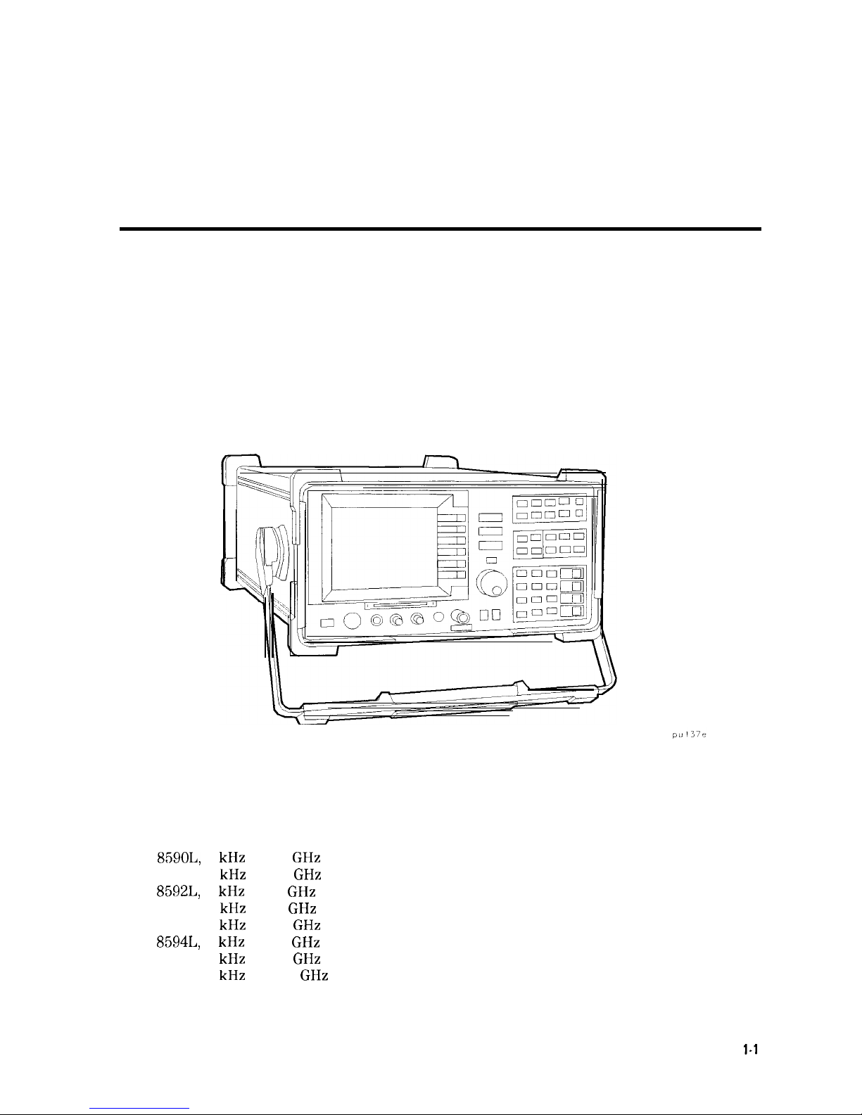
l-l. HP 8590 Series Spectrum Analyzer

.....................

1-2. Setting the Line Voltage Selector Switch

...................

l-3. Checking the Line Fuse

..........................

l-4. Reference Connector

............................

1-5. Example of a Static-Safe Work Station

...................

2-l. Front-Panel Feature Overview

.......................

2-2. Rear-Panel Feature Overview

........................

2-3. Adjusting the Fine Focus

..........................

2-4. Screen Annotation

.............................

2-5. Relationship between Frequency and Amplitude

...............

2-6. Reading the Amplitude and Frequency

...................

2-7. Inserting the Memory Card

.........................

2-8. Memory Card Battery Date Code Location

..................

2-9. Memory Card Battery Replacement

.....................

2-10. Rear-Panel Battery Information Label

....................

3-l. Set-Up for Obtaining Two Signals

......................

3-2. Resolving Signals of Equal Amplitude

....................

3-3. Resolution Bandwidth Requirements for Resolving Small Signals

.......

3-4. Signal Resolution with a 10 kHz Resolution Bandwidth

............

3-5. Signal Resolution with a 30 kHz Resolution Bandwidth

............

3-6. IJsing the Marker Counter

.........................

3-7. After Zooming In on the Signal

.......................

3-8. Peaking Signal Amplitude Using Preselector Peak

..............

3-9. Using Marker Tracking to Track an Unstable Signal

.............

3-10. Viewing an Unstable Signal Using Max Hold A

................

3-l 1. Viewing an Unstable Signal With Max Hold, Clear Write, and Min Hold

....

3-12. Placing a Marker on the CAL OUT Signal

..................

3-13. Using the Marker Delta Function

......................

3-14. Using the Marker to Peak/Peak Function

..................

3-15. Frequency and Amplitude Difference between Signals

............

3-16. Low-Level Signal

.............................

3-17. Using 0 dB Attenuation

..........................

3-18. Decreasing Resolution Bandwidth

......................

3-

19. Decreasing Video Bandwidth

........................

3-20. Using the Video Averaging Function

....................

3-2 1. Harmonic Distortion

............................

3-22. RF Attenuation of 10

dB

..........................

3-23. No Harmonic Distortion

..........................

3-24. Third-Order Intermodulation Equipment Setup

...............

3-25. Measuring the Distortion Product

......................

3-26. Viewing an AM Signal

...........................

3-27. Measuring Modulation in Zero Span

.....................

3-28. Using Harmonic Lock

...........................

3-29. Harmonic Locking Off

...........................

4-l. FFT Annotation

..............................

4-2. Percent Amplitude Modulation Measurement

................

l-l
1-4
1-5
1-8

l-11

2-2
2-5

2-9
2-10
2-14
2-15

2-19
2-20
2-21
2-22

3-2

3-3
3-4
3-5
3-5

3-6

3-7

3-8

3-10
3-11
3-11
3-12
3-13
3-13
3-14
3-15
3-16
3-16
3-17
3-19

3-20

3-21

3-21

3-22

3-23
3-25
3-25

3-27

3-27

4-2

4-5

Contents-7

4-3. Block Diagram of a Spectrum Analyzer/Tracking-Generator Measurement System

4-7

4-4. Transmission Measurement Test Setup

....................

4-8

4-5. Tracking-Generator Output Power Activated

.................

4-9

4-6. Spectrum Analyzer Settings According to the Measurement Requirement

...

4-9

4-7. Decrease the Resolution Bandwidth to Improve Sensitivity

..........

4-10

4-8. Manual Tracking Adjustment Compensates for Tracking Error

........

4-10

4-9. Normalized Trace

.............................

4-11

4-10. Measure the Rejection Range with Delta Markers

..............

4-12

4-l 1. Demodulation of an FM Signal

.......................

4-13

4-12. Continuous Demodulation of an FM Signal

..................

4-14

4-13. Triggering on an Odd Field of a Video Format

................

4-15

4-14. Triggering on an Even Field of a Video Format

...............

4-16

4-15. Reflection Measurement Short Calibration Test Setup

.............

4-17

4-16. Measuring the Return Loss of the Filter

...................

4-18

4-

17. Time-Gate Utility Display

..........................

4-19

4-18. Viewing Time-Sharing of a Frequency with an Oscilloscope

..........

4-23

4-19. Viewing Time-Sharing of a Frequency with a Spectrum Analyzer

.......

4-24

4-20. Pulse Repetition Interval and Pulse Width (with Two Signals Present)

.....

4-25

4-21. Test Setup for Option 105

.........................

4-27

4-22. Setting the Center Frequency, Span, and Reference Level

..........

4-28

4-23. Setting the Sweep Time

..........................

4-28

4-24. Setting the Gate Delay and Gate Length Using an Oscilloscope

........

4-29

4-25. Using Time-Gating to View Signal 1

.....................

4-30

4-26. Placing the Gate Output During the Second Signal

..............

4-31

4-27. Viewing Both Signals with Time-Gating

...................

4-32

4-28. Gate Not Occurring During the Pulse

....................

4-33

4-29. Gate is Occurring at the Beginning of the Pulse

...............

4-33

4-30. Self-Calibration Data Results

........................

4-36

4-31. Rear Panel Connections for Option 105

...................

4-36

4-32. Gate On

..................................

4-37

4-33. Using the Level Gate Control

........................

4-38

4-34. N dB Bandwidth Measurement

.......................

4-39

4-35. Percent Amplitude Modulation Measurement

................

4-40

4-36. Third-Order Intermodulation Measurement

.................

4-42

4-37. Occupied Bandwidth

............................

4-44

4-38. Adjacent Channel Power

..........................

4-46

4-39. Adjacent Channel Power Extended

.....................

4-46

4-40. Adjacent Channel Power Graph

.......................

4-47

4-41. Channel Power

..............................

4-48

4-42. Channel Power Graph

...........................

4-49

5-1. Marker

‘Ihble

Display

............................

5-2

5-2. Peak

‘Ihble

Display

.............................

5-4

5-3. Inserting the Memory Card

.........................

5-11

5-4. Typical Limit-Line Display

.........................

5-19

5-5. The Completed Limit-Line Table

......................

5-21

5-6. Limit-Line Segments

............................

5-24

5-7. Segment Types

..............................

5-27

5-8. Upper and Lower Limit-Line Testing

....................

5-30

5-9. Analog+ Display Mode

...........................

5-32

5-10. Windows Display Mode

...........................

5-33

5-

11. Amplitude-Correction Display

.......................

5-35

5-

12. Completed Amplitude-Correction

Iable

...................

5-37

5-13. Amplitude-Correction Points

........................

5-38

6-1. Three Printouts Per Page

..........................

6-2

6-2. Plots Per Page

...............................

6-3

Contents-8

6-3.

ThinkJet

Printer Switch Settings

......................

6-4

6-4. HP-IB to Centronics Converter Setup

....................

6-5

6-5. Printer Configuration Menu Map

......................

6-5

6-6. HP 7475A Plotter Switch Settings

......................

6-7

6-7. Plot Configure Menu

............................

6-8

6-8. 9600 Baud Settings for Serial Printers

....................

6-11

6-9. Printer Configure Menu

..........................

6-12

6-10. Connecting the HP

7550A/B

Plotter

.....................

6-15

6-l 1. Baud Rate Menu Map

...........................

6-15

6-12. Plot Configure Menu

............................

6-16

6-13. Parallel Printer Switch Settings

.......................

6-18

6-14. Printer Configuration Menu Map

......................

6-19

6-15. Plot Configure Menu

............................

6-22

7-l. Memory Card Catalog Information

.....................

7-17

7-2. Analyzer Memory Catalog Information

...................

7-18

7-3. CATALOG ON EVENT Display

.......................

7-20

7-4. Connecting a Printer to the Spectrum Analyzer

...............

7-29

Contents-9

lhbles

l-l. Accessories Supplied with the Spectrum Analyzer

..............

1-2. Power Requirements

............................

l-3. AC Power Cables Available

.........................

1-4. Static-Safe Accessories

...........................

2-l. RF Output Frequency Range

........................

2-2. Screen Annotation

.............................

2-3. Screen Annotation for Trace, Trigger, and Sweep Modes

...........

4-1. Determining Spectrum Analyzer Settings for Viewing a Pulsed RF Signal

...

4-2. Pulse Generator Test Setup Settings

.....................

4-3. Signal Generator Test Setup Settings

....................

4-4. Gate Delay, Resolution Bandwidth, Gate Length, and Video Bandwidth Settings
4-5. Sweep Time Settings

............................

5-1. Summary of Save and Recall Operations, Analyzer Memory ..........

5-2. Comparison of Analyzer Memory and Memory Card Operations

........

5-3. Save and Recall Functions Using Memory Card

...............

5-8. External Keyboard Functions

........................

7-1. Commands Not Available with Analog+ Operation ..............

7-2. Center Frequency and Span Settings for Harmonic Bands

..........

7-3. Memory Card Catalog Information

.....................

7-4. Analyzer Memory Catalog Information *

...................

7-5. CATALOG ON EVENT Display Description ..................

7-6. Default Configuration Values

........................

7-7. Compatibility of FFT With Other Functions .................

7-8. Commands Altered/Not Available within the Gate Utility

...........

7-9. Functions Which Exit The Windows Display Format

.............

7-10. Model Specific Preset Conditions

......................

7-

11. Common Preset Conditions

.........................

7-12. Preset Spectrum Conditions for All Models

7-13. HP 85933, HP

8594E,

HP 85953, and HP 8596E : : : : : : : : : : : : : :

:

9-1. Hewlett-Packard Sales and Service Offices ..................

A-l. Status Byte Definition

...........................

1-3
1-4
1-7

1-12

2-4
2-11
2-12
4-26
4-27
4-28

4-34

4-35

5-9

5-10

5-17
5-40

7-9
7-12
7-17
7-19
7-20

7-32

7-43

7-47
7-61

7-66
7-67
7-68
7-71

9-5

A-2

Contents-l 0

1

Preparing For Use

What You’ll Find in This Chapter

This chapter describes the process of getting the spectrum analyzer ready to use when you
have just received it. See “Preparing Your Spectrum Analyzer For Use” for the process steps.
The process includes initial inspection, setting up the unit for the selected ac power source,
and performing automatic self-calibration routines. Information about static-safe handling
procedures is also included in this chapter.

Introducing the HP 8590 Series Spectrum Analyzers

Figure l-l. HP 8590 Series Spectrum Analyzer

The HP 8590 Series spectrum analyzers are small, lightweight test instruments that cover the
RF and microwave frequency ranges:

HP

859OL,

9

kHz to 1.8

GHz

HP

85913,

9

kHz to 1.8

GHz

HP

8592L,

9

kHz

to 22

GHz

HP

85933,

9

kHz

to 22

GHz

HP

85943,

9

kHz to 2.9

GHz

HP

8594L,

9

kHz

to 2.9

GHz

HP

85953,

9

kHz to 6.5

GHz

HP

85963,

9

kHz

to 12.8

GHz

Preparing For Use

l-1

Preparing Your Spectrum Analyzer for Use

Detailed information for all of the steps in this process is included in this chapter.

1. Unpack the spectrum analyzer and inspect it.

2. Verify that all of the accessories and documentation has been shipped.

3. Check that the line voltage selector is set to the proper voltage.

4. Check that the correct fuse is in place.

Warning

Failure to ground the spectrum analyzer properly can result in personal
injury. Use an ac power outlet that has a protective earth contact.

DO

NOT defeat the earth grounding protection by using an extension cable,

power cable, or autotransformer without a protective ground conductor.

Caution

Do

not connect ac power until you have verified that the line voltage is correct,

the proper fuse is installed, and the line voltage selector switch is properly
positioned, as described in the following paragraphs. Damage to the equipment
could result.

5. Connect the power cable to the spectrum analyzer and turn it on.

Warning

Install the product so that the detachable power cord is readily

identifiable and easily reached by the operator. The detachable power
cord is the product disconnecting devise. It disconnects the mains

circuits from the mains supply before other parts of the product. The
front panel switch is only a standby switch and is not a LINE switch.
Alternatively, an externally installed switch or circuit breaker (which is
readily identifiable and is easily reached by the operator) may be used as a
disconnecting device.

6. Execute the self-calibration routines.

1-2 Preparing For Use

Initial Inspection

Inspect the shipping container for damage. If the shipping container or cushioning material is
damaged, keep it until you have verified that the contents are complete and you have tested
the spectrum analyzer mechanically and electrically.

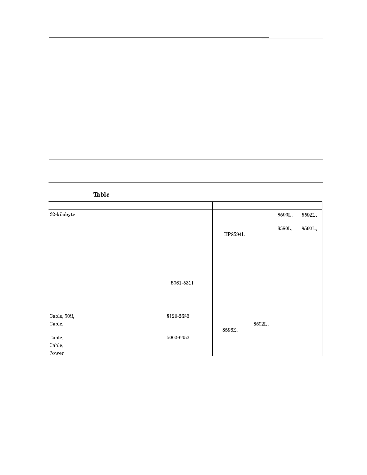
Table l-l contains the accessories shipped with the spectrum analyzer. If the contents are
incomplete or if the spectrum analyzer does not pass the verification tests in the calibration

guide, notify the nearest Hewlett-Packard office. If the shipping container is damaged or the

cushioning material shows signs of stress, also notify the carrier. Keep the shipping materials
for the carrier’s inspection. The HP office will arrange for repair or replacement without
waiting for a claim settlement.

If the shipping materials are in good condition, retain them for possible future use. You may
wish to ship the spectrum analyzer to another location or to return it to Hewlett-Packard for
service. See “How to Return Your Analyzer for Service,”

in Chapter 9 for more information

about shipping materials.

Note

If cleaning is necessary, use a damp cloth only.

lhble

l-l. Accessories Supplied with the Spectrum Analyzer

Description

HP Part Number

32-kilobyte Memory Card

0950-1964

Memory Card Holder

9222-1545

Adapter, Type N (m) to BNC (f)

1250-0780

Two Adapters, BNC (m) to BNC (f)

1250-0076

Adapter, BNC (m) to SMA (f)

HP 1250-1700

Connector, APC-3.5 mm (f) to (f)

HP

5061-5311

Reference Connector

1250-1499

Zable, 5OQ,

BNC

8120-2682

Zable,

SMA (m) to type N (m)

8120-5148

Zable,

750, BNC

5062-6452

Zable,

SMA (m) to SMA (m)

08592-60061

‘ower

cable

See Table 1-3

Comments

Shipped with analyzer. HP

859OL,

HP

8592L,

and HP 8594L must include Option 003.

Shipped with analyzer. HP

859OL,

HP

8592L,

and HP8594L must include Option 003.

Not shipped with Option 001. Two adapters

are shipped with Option 010.

Shipped with Option 105 only. The adapters
can be used to connect cables to the
rear-panel connectors.

Shipped with Option 026 only.
Shipped with Option 026 only.
Shipped connected between the 10 MHz REF

OUT and the EXT REF IN on the rear panel of
the analyzer. Not shipped with HP 8590L
option 713.

Not shipped with Options 001, 011, or 026.
Shipped with HP

8592L,

HP 85933, and

HP

85963.

Not shipped with Option 026.
Shipped with Options 001 or 011 only.
Shipped with Option 026 only.
Shipped with analyzer.

Preparing For Use 1-3

Power Requirements

The spectrum analyzer is a portable instrument and requires no physical installation other than
connection to a power source.

Warning

Failure to ground the spectrum analyzer properly can result in personal
injury. Use an ac power outlet that has a protective earth contact. DO

NOTdefeat

the earth grounding protection by using an extension cable,

power cable, or autotransformer without a protective ground conductor.

Caution

Do not connect ac power until you have verified that the line voltage is correct,
the proper fuse is installed, and the line voltage selector switch is properly
positioned, as described in the following paragraphs. Damage to the equipment
could result.

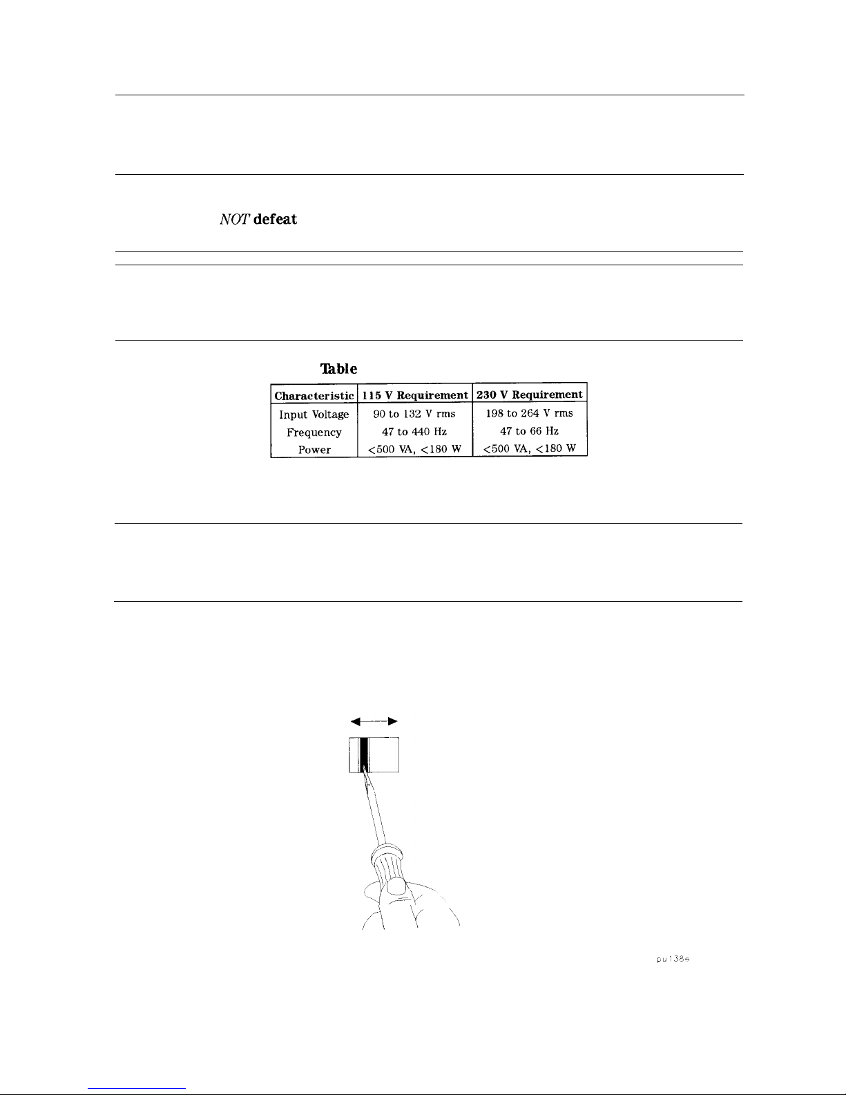
‘Ihble

1-2. Power Requirements

Setting the Line Voltage Selector Switch

Caution

Before connecting the spectrum analyzer to the power source, you must set the
rear-panel voltage selector switch correctly to adapt the spectrum analyzer
to the power source. An improper selector switch setting can damage the
spectrum analyzer when it is turned on.

Set the instrument’s rear-panel voltage selector switch to the line voltage range
(115 V or 230 V) corresponding to the available ac voltage. See Figure l-2. Insert a small
screwdriver or similar tool in the slot and slide the switch so that the proper voltage label is
visible.

,,*-\, ‘I/ “\

Figure l-2. Setting the Line Voltage Selector Switch

1-4 Preparing For Use

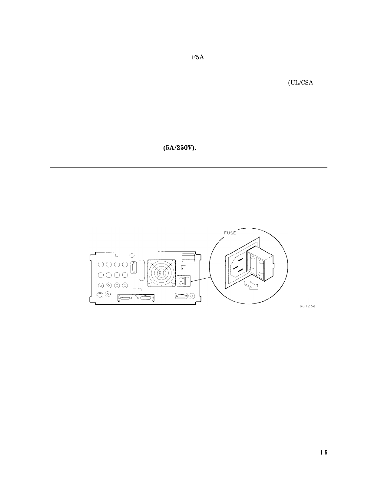
Checking the Fuse

The recommended fuse is size 5 by 20 mm, rated

F5A,

250 V (IEC approved). This fuse may be

used with input line voltages of 115 V or 230 V. Its HP part number is 2110-0709.

With an input line voltage of 115 V an alternate fuse can be used. In areas where the
recommended fuse is not available, a size 5 by 20 mm, rated fast blow, 5 A, 125 V (ULXSA
approved) fuse may be substituted. Its HP part number is 2110-0756.

The line fuse is housed in a small container beside the rear-panel power connector. See
Figure l-3. The container provides space for storing a spare fuse, as shown in the figure.

To check the fuse, insert the tip of a screwdriver in the slot at the middle of the container and
pry gently to extend the container.

Warning

For continued protection against fire hazard replace line fuse only with

same type and rating

(5A/250V).

The use of other fuses or material is

prohibited.

Note

The fuse container is attached to the line module; it cannot be removed.

The fuse closest to the spectrum analyzer is the fuse in use. If the fuse is defective or missing,
install a new fuse in the proper position and reinsert the fuse container.

Figure l-3. Checking the Line Fuse

Preparing For Use

l-5

Power Cable

The spectrum analyzer is equipped with a three-wire power cable, in accordance with
international safety standards. When connected to an appropriate power line outlet, this cable
grounds the instrument cabinet.

Warning

Failure to ground the spectrum analyzer properly can result in personal
injury. Before turning on the spectrum analyzer, you must connect its
protective earth terminals to the protective conductor of the main power
cable. Insert the main power cable plug only into a socket outlet that has

a protective earth contact. DO NOT defeat the earth-grounding protection

by using an extension cable, power cable, or autotransformer without a
protective ground conductor.

If you are using an autotransformer, make sure its common terminal is

connected to the protective earth contact of the power source outlet
socket.

Various power cables are available to connect the spectrum analyzer to the types of ac power
outlets unique to specific geographic areas. The cable appropriate for the area to which the
spectrum analyzer is originally shipped is included with the unit. You can order additional ac
power cables for use in different areas.

Table

l-3 lists the available ac power cables, illustrates

the plug configurations, and identifies the geographic area in which each cable is appropriate.

1-6 Preparing For Use

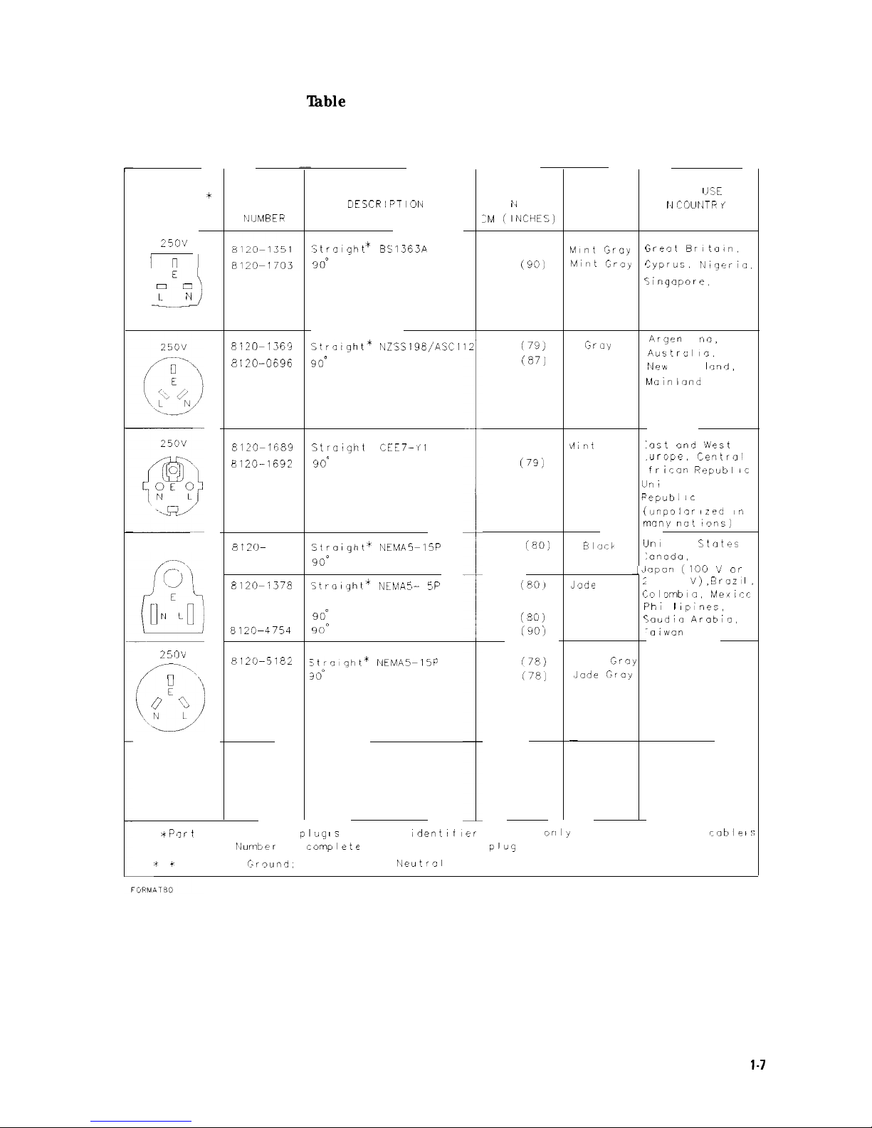
lhble

1-3. AC Power Cables Available

CABLE
L E rl G T H

:M ~INCHEC,)

FOR

IJSE

I II

COUI‘JTR i

CABLE

HP PART

rIIJMl3ER

PLUG

DESCRIPTI’JN

CABLE
COLOR

PLUG TYPE * *

25O’J

Strnight

BS1363A

9om

229 (90)
229

(90)

Mint Gray

Mint Gray

;reot Brltuin.
:yprus,

I‘Nigerin.
;ingnpore,

Zimbabwe

c
/

<

E
E

A

L

F

(
r

i

C

_J

;
(

F
‘

1

E

A

0 0

L

N

8120~1363
8 120-0696

Strn,ght*

NZSSlSB/ASCl

9o”

12

~

201

(79)

221

(87)

Grily

Gray

Argen

t i

~10,
Auitrulla,
New

Zen I

anJ,

Mainland

China

8120~1683
E120-1692

Stratght

*

CEE7-II

1

9o”

201 (79)

201

(79j

i4lnt

Gray

Mint Gray

:ast and \Nest
.urope,

Centrnl

fricon Replubl ic

InI

ted Arab

‘epubl IC

unpnlnrized

I”

nnny not 19ns)

I

125V

8 120-

1348

Straight*

NEMA5S15P

8120-1538

9o”

203

(80)

203 (80)

In,

ted

States

:anocla,

apon (100 $4

0,~

‘00

V), eraz I,

;olombia.

Mexlcr

‘hl

I I

spines,

<audio Arobin,

-0iwan

Blnck

Block

Jade

Gray
Jade Gray
Jade Gray
Jade Gray

8120-1378

Straight*

NEMA5-

1

:P

8 120-4753 Straight

8120-1521

go0

8120-4754

9oa

203

(80)

230 (90)

203

(80)

230

(9Oj

25O’d

8120-5182

stro1gt,t*

NEMA5S15P

8120-5181

30*

200

(78)

200

(78)

Israel

Jade

Grny

.Jade Gray

-

,A---,

i :

(:

.\f\ ‘”

ii Pnrt

number for

pluq IS

industry

Identifier

for plug

orlly

Number shown for

cable I:;

HP Port

rlurnber

for

complrie

cable, including

pll~g

ii #

E = Earth

Lr~und:

L = Line, N =

r>leutraI

Preparing For Use

l-7

Turning on the Analyzer for the First Time

When you turn the spectrum analyzer on for the first time, you should perform frequency and
amplitude self-calibration routines to generate correction factors and indicate that the unit is
functioning correctly. The spectrum analyzer should be allowed to warm-up for 30 minutes
before performing the self-calibration routines. See “When Is Self-Calibration Needed?”
in Chapter 2 for helpful guidelines on how often the self-calibration routines should be
performed.

Perform the following steps:

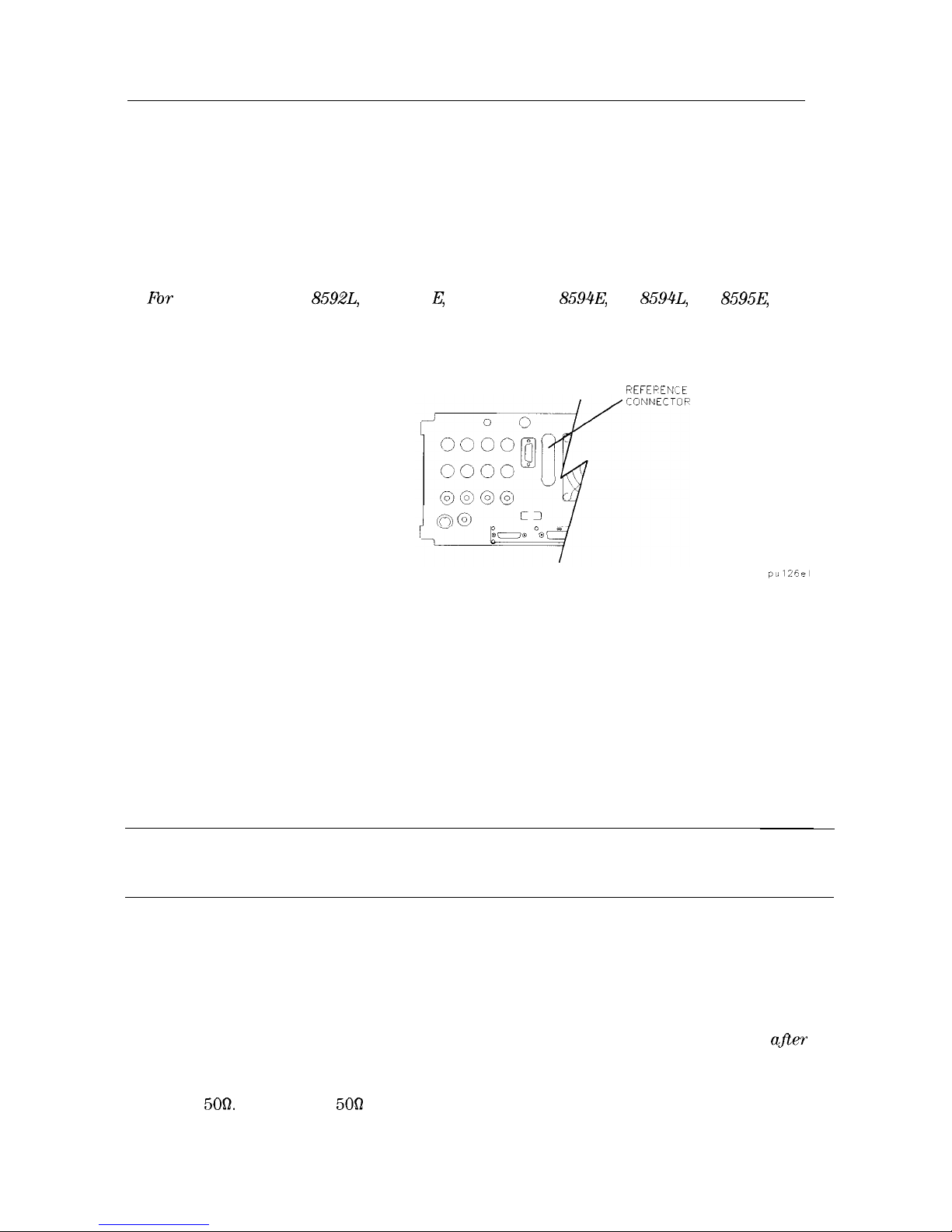
1. Fbr an HP 85901, HP

8592L,

HP 8591 E, HP 85933, HP

8594E,

HP

8594L,

HP

8595E,

or

HP 85963 ensure the reference connector is connected between the 10 MHz OUTPUT and

EXT REF IN rear-panel connectors. See Figure l-4.

REFEPENCE

Figure 1-4. Reference Connector

If you wish to use an external 10 MHz source as the reference frequency, disconnect the
reference connector from the rear-panel and connect an external reference source to the
EXT REF IN connector on the rear panel.

2. Plug the power cord into the spectrum analyzer.

3.

Press (LINE).

After a few seconds, the screen displays the firmware revision date in the YYMMDD format.
For example, 930522 indicates May 22, 1993. This is a change from previous revisions where
any firmware date used the DDMMYY format prior to 930506.

Note

Record the firmware date and keep it for reference. If you should ever need to
call Hewlett-Packard for service or with any questions regarding your spectrum
analyzer, it will be helpful to have the firmware date readily available.

If your spectrum analyzer is equipped with Option 021 (HP-IB interface), the appropriate
interface address (HP-IB ADRS : XX) also appears on the screen.

If your spectrum analyzer is equipped with Option 023 (RS-232 interface), the baud rate
(RS232 : XXXX) is displayed.

4. To meet spectrum analyzer specifications, allow a 30 minute warm-up before attempting to

make any calibrated measurements. Be sure to calibrate the spectrum analyzer only afler
the spectrum analyzer has met the operating temperature conditions.

5. Connect the type N (m) to BNC (f) connector (shipped with the spectrum analyzer) to the
INPUT

5OQ.

Connect the 500 coaxial cable (also shipped with the instrument) between the

front-panel CAL OUT and the INPUT 500 connector. If the spectrum analyzer has Option

1-8 Preparing For Use

001

(7562

input), use the 750 calibration cable shipped with the analyzer. Use only 750

connectors to avoid damage to the RF input connector.

Note

Option 105 only: Remove all connections to the GATE TRIGGER INPUT

rear-panel connector before performing the self-calibration routines.

6. Perform the frequency and amplitude self-calibration routine by pressing (CAL) and
CAL FREQ & AMPTD . During the frequency routine, CAL: SWEEP, CAL: FREQ, and CAL: SPAN

are displayed as the sequence progresses. For an Option 102, CAL: FM GAIN + OFFSET is also
displayed.

During the amplitude routine, CAL; AMPTD, CAL: 3 dB BW, CAL:

ATTEN,

and CAL:

LOGAMP

are

displayed as the sequence progresses. CAL: DONE appears when the routine is completed.

Any failures or discrepancies produce a message on the screen; see Chapter 9.

7. When the frequency and amplitude self-calibration routines have been completed
successfully, store the correction factors by pressing CAL STORE.

The self-calibration routines calibrate the spectrum analyzer by generating correction factors.
The

softkey

CAL STORE stores the correction factors in the area of spectrum analyzer

memory that is saved when the spectrum analyzer is turned

off;

the spectrum analyzer will

automatically apply these factors in future measurements. If CAL STORE is not pressed, the
correction factors remain in effect until the spectrum analyzer is turned off.

Performing the Tracking-Generator Self-Calibration Routine

For spectrum analyzers with Option 010 or 011, the tracking-generator self-calibration routine
should be performed prior to using the tracking generator.

Note

Since the tracking generator calibration routine depends on the accuracy of
the absolute amplitude level of the spectrum analyzer, the spectrum analyzer

amplitude calibration should be done prior to using CAL TRK GEM .

1. To calibrate the tracking generator, connect the tracking generator output (RF OUT

5OR)

to
the spectrum analyzer INPUT 500 connector, using an appropriate cable and BNC-to-Type
N adapters. If the spectrum analyzer has Option 001 (750 input), use the

75Q

calibration

cable shipped with the analyzer. Use only

75fl

connectors to avoid damage to the RF input

connector.

Note

A low-loss cable should be used for accurate calibration. Use the

509

cable
shipped with the spectrum analyzer. If the analyzer has Option 001 (75n input),
use the

75R

cable shipped with the spectrum analyzer.

2. Press the following spectrum analyzer keys:

m),

More 1 of 4 , More 2 of 4 , then

CAL TRK GEN . TG SIGNAL NOT FOUND will be displayed if the tracking generator output is

not connected to the spectrum analyzer input.

3. To save this data in the area of spectrum analyzer memory that is saved when the spectrum
analyzer is turned off, press CAL STORE .

Preparing For Use 1-9

Performing the YTF Self-Calibration Routine

For preselected spectrum analyzers (HP

8592L,

HP 85933, HP

8595E,

and HP 85963) only, the
yig-tuned filter (YTF) self-calibration routine should be performed periodically. See “When Is
Self-Calibration Needed?” in Chapter 2 for helpful guidelines on how often the self-calibration
routines should be performed.

To perform the YTF self-calibration routine, use the following procedure:

1. Connect a low-loss cable (such as HP part number 8120-5148) from 100 MHz COMB OUT to
the spectrum analyzer input. For the HP 85953, use the CAL OUT, instead of the COMB

OUT, as the spectrum analyzer input.

2. Press (CAL) then CAL YTF . The YTF self-calibration routine completes in approximately:

Model Number YTF Cal Time

HP 8592L

7 minutes

HP 85933

7

minutes

HP

85953

3

minutes

HP

85963

5

minutes

3. Press (CAL) then CAL STORE

_

When the self-calibration routines have been completed successfully, the spectrum analyzer is

ready for normal operation.

l-1 0

Preparing For Use

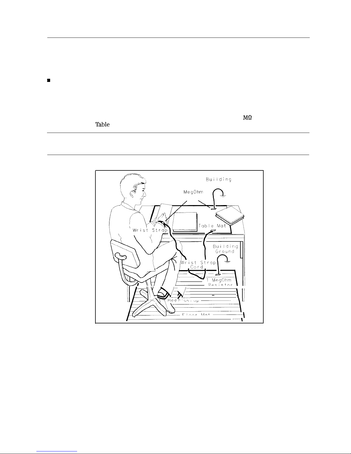
Electrostatic Discharge

Electrostatic discharge (ESD) can damage or destroy electronic components. All work on
electronic assemblies should be performed at a static-safe work station. Figure l-5 shows an
example of a static-safe work station using two types of ESD protection:

H

Conductive table-mat and wrist-strap combination.

n Conductive floor-mat and heel-strap combination.

Both types, when used together, provide a significant level of ESD protection. Of the two, only

the table-mat and wrist-strap combination provides adequate ESD protection when used alone.

To ensure user safety, the static-safe accessories must provide at least 1 MR of isolation from
ground. Refer to

‘fable

l-4 for information on ordering static-safe accessories.

Warning

These techniques for a static-safe work station should not be used when
working on circuitry with a voltage potential greater than 500 volts.

BUI lding

Ground

1

MegOhm

Resistor

1

q&-

-

\Il

mtiee I

St rap

k

AU

/./-xYD

” -

Floor Mat

-\

-~I

Figure 1-5. Example of a Static-Safe Work Station

Preparing For Use

l-l 1

Reducing Damage Caused by ESD

The following suggestions may help reduce ESD damage that occurs during testing and
servicing operations.

n Before connecting any coaxial cable to an spectrum analyzer connector for the first time each

day, momentarily ground the center and outer conductors of the cable.

w

Personnel should be grounded with a resistor-isolated wrist strap before touching the center

pin of any connector and before removing any assembly from the unit.

n Be sure that all instruments are properly earth-grounded to prevent a buildup of static

charge.

Table

l-4 lists static-safe accessories that can be obtained from Hewlett-Packard by using the

HP part numbers shown.

‘Ihble

1-4. Static-Safe Accessories

HP Part
Number

Description

9300-0797

Set includes: 3M static control mat 0.6 m x 1.2 m (2 ft x 4 ft) and 4.6 cm
(15 ft) ground wire. (The wrist-strap and wrist-strap cord are not included.
They must be ordered separately.)

9300-0980
9300-1383

9300-l 169

Wrist-strap cord 1.5 m (5 ft)
Wrist-strap, color black, stainless steel, without cord, has four adjustable

links and a 7 mm post-type connection.
ESD heel-strap (reusable 6 to 12 months).

1.12

Preparing For Use

2

Getting Started

What You’ll Learn in this Chapter

This chapter introduces the basic functions of the HP 8590 Series spectrum analyzers. In this

chapter you will:

w

Get acquainted with the front-panel and rear-panel features.

n Get acquainted with the menus and softkeys.

w

Learn about screen annotation.

n Make a basic measurement (the calibration signal).
n Learn how to improve measurement accuracy by using self-calibration routines.
n Learn how to insert the memory card and about the memory card battery.
n Learn about the spectrum analyzer battery.

Note

Before using your spectrum analyzer, please read Chapter 1 “Preparing for
Use,” which describes how to set up your spectrum analyzer and how to verify
that it is operational. Chapter 1 describes many safety considerations that
should not be overlooked.

Getting Acquainted with the Analyzer

Front-Panel Features

The following section provides a brief description of front-panel features. Refer to Figure 2-l.

1

Active function block is the space on the screen that indicates the active function. Most

functions appearing in this block can be changed using the knob, step keys, or data keys.

2

Message block is the space on the screen where

MEAS

UNCAL and the asterisk

(*)

appear.

If one or more functions are manually set (uncoupled), and the amplitude or frequency
becomes uncalibrated,

MEAS

UNCAL appears. (Use

[AUTO COUPLE]

and AUTO ALL to

recouple functions.) The asterisk indicates that a function is in progress.

3

Softkey

labels are the annotation on the screen next to the unlabeled keys. Most of the

labeled keys on the spectrum analyzer front panel (also called front-panel keys) access
menus of related softkeys.

4

Softkeys

are the unlabeled keys next to the screen.

Getting Started 2-1

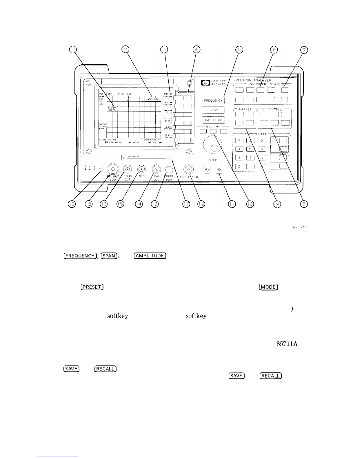
Figure 2-l. Front-Panel Feature Overview

5

[FREQUENCY],

ISPAN),

and

@Kii%ZE]

are the three large dark-gray keys that activate the

primary spectrum analyzer functions and access menus of related functions.

6

INSTRUMENT STATE functions affect the state of the entire spectrum analyzer.

Self-calibration routines and special-function menus are accessed with these keys. The
green

@‘EZi]

key resets the spectrum analyzer to a known state. The

m

key
accesses the current operating mode of the spectrum analyzer and allows you to change
to any operating mode available for your spectrum analyzer. All spectrum analyzers

have the spectrum analyzer mode of operation (indicated by SPECTRUM ANALYZER

).

If an additional

softkey

label appears in the

softkey

label area, a program (also called
a downloadable program or personality) has been loaded into the spectrum analyzer
memory. This document covers the spectrum analyzer mode of operation only; consult
the documentation accompanying the specific measurement personality that you are
using for information about other modes of operation. (For example: the HP

857llA

Cable Television Measurements Personality, the HP 85713A Digital Radio Measurements
Personality, or the HP 85715A GSM Measurements Personality.)

m

and

[?EXE]

keys save and recall traces, states, limit-line tables, amplitude

correction factors, and programs to or from a memory card.

ISAVE)

and

[RECALL)

keys also
save and recall traces, states, limit-line tables, and amplitude correction factors to or
from the spectrum analyzer memory.

2-2 Getting Started

Note

If you wish to reset the spectrum analyzer configuration to the state it was in
when it was originally shipped from the factory, use DEFAULT

CONFIG

. Refer

to the DEFAULT

CONFIG softkey

description in Chapter 7 for more information.

7

8

9

10

11

12

Icopv)

prints or plots screen data. (This requires Option 041 or 043.) Use

@ZiK$

Plot Conf

ig

or Print Conf

kg,

and COPY DEV PRMT PLT before using

Icopv).

See

Chapter 7 for more details.
CONTROL functions access menus that allow you to adjust the resolution bandwidth,

adjust the sweep time, store and manipulate trace data, and control the instrument
display.

MARKER functions control the markers, read out frequencies and amplitudes along the
spectrum-analyzer trace, automatically locate the signals of highest amplitude, and keep
a signal at the marker position in the center of the screen.

WINDOWS keys, turn on the windows display mode. They allow switching between
windows and control the zone span and location.

Fbr

the HP

859ZE,

HP

8593E,

HP

8594E,

HP

8595E,

and HP 85963 only.

HOLD key. Fbr the HP

859OL,

HP

8592L,

and HP 8594L only.

[HOLD]

deactivates an

active function. For the HP 85913, HP

8593E,

HP 85943, HP

8595E,

and HP

8596E,

the

“hold” function is available as the HOLD

softkey

under

cm).

DATA keys, STEP keys, and knob allow you to change the numeric value of an active
function.

INPUT 500 is the signal input for the spectrum analyzer. (INPUT

75Q

is the signal input

for an Option 001 spectrum analyzer.)

-

Caution

Excessive signal input will damage the spectrum analyzer input attenuator and
input mixer. Use extreme caution when using the spectrum analyzer around
high-power RF sources and transmitters. The maximum input power that the
spectrum analyzer can tolerate appears on the front panel and should not be
exceeded.

Excessive dc voltage can also damage the input attenuator. For your particular
instrument, note the maximum de voltage that should not be exceeded on the
spectrum analyzer front panel (beneath the INPUT

5OQ

connector).

13

PROBE PWR provides power for high-impedance ac probes or other accessories.

14

CAL OUT provides a calibration signal of 300 MHz at -20

dBm

(29

dBmV

for Option 001

or 011).

15

VOL-INTEN or INTENSITY. For the HP 85913, HP

8593E,

HP 85943, HP 85953, or

HP 8596E only. The VOL-INTEN knob changes the brightness of the display. If Option

102, 103, or 110 is installed, it can also adjust the volume of the internal speaker. If it
adjusts both, the inside part of the knob adjusts the intensity while the outside part
adjusts the volume.

The INTENSITY knob changes the brightness of the display. For the HP

859OL,

HP

8592L,

and HP 8594L only.

Getting Started 2-3

16

100 MHz COMB OUT supplies a 100 MHz reference signal that has harmonics up to

22

GHz. Fbr

the HP 85921, HP

8593E,

or HP 8596E only.

17

Memory card reader reads from or writes to a memory card. The memory card reader is

standard with an HP 85913, HP 85933, HP 85943, HP 85953, and HP 85963. It is also
available for the HP

859OL,

HP

8592L,

and HP 8594L as Option 003.

18

RF OUT

5OD

supplies a source output for the built-in tracking generator.

Fbr Option 010 only. See

liable

2-l.

Caution

If the tracking generator output power is too high, it may damage the device
under test. Do not exceed the maximum power that the device under test can
tolerate.

RF OUT 750 supplies a source output for the built-in tracking generator.

For Option 011 only. See lbble 2-l.

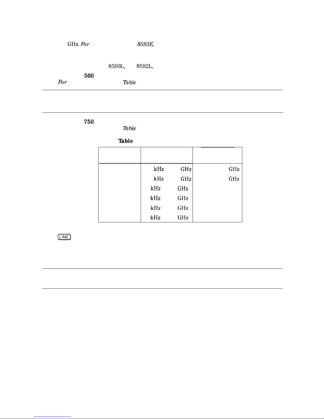
‘able

2-l. RF Output Frequency Range

Model Number

HP 8590L 100 kHz to 1.8

GHz

HP 85913

100 kHz to 1.8

GHz

HP 85933 9 kHz to 2.9

GHz

HP 85943 9 kHz to 2.9

GHz

HP 85953 9 kHz to 2.9

GHz

HP 85963 9 kHz to 2.9

GHz

Option 010

Frequency Range

Option 011

Frequency Range

1 MHz to 1.8

GHz

1 MHz to 1.8

GHz

not available
not available
not available
not available

19

ILINE)

turns the instrument on and off. The symbols to the left of the line switch
represent the up position of the switch when the instrument is off, and the down
position of the switch when the instrument is on. An instrument self-check is performed
every time the instrument is turned on. After applying power, allow the temperature of

the instrument to stabilize for best measurement results.

Note

The instrument continues to draw power when it is plugged into the ac power
source even if the line power switch is off.

2-4 Getting Started

Rear-Panel Features

I

KY

LO

OUT

WE

P+

TU E

i

AUX

SWEEP

HIGH SWEEP

VIDEO

OUTPVT N/OUT

CTTLj

OUTPUT

cm

m

63

SEP

OPT

B

p ,“K,“ER

-\1

In-

FUSE

\I

I

‘W

w

\vJ

ye

\

MON I T

A

Ill

I

(I

EXJ TRlG I

I

r--7

._.. _

AUX INTE

ACE ““TPUT

IN UT(TTLj

EXT

YBOARD

~

\

(3

/

\:

,0/d-

@

SD

fiy<

\~~~~

OPTlOh

041

OPTION 043

Figure 2-2. Rear-Panel Feature Overview

1

EXT ALC INPUT allows the use of an external detector or power meter for automatic

leveling control of the tracking generator. Fbr an HP 8590L and HP 8591E Option 010 or

011 only. Allows the use of an external detector for an HP

85934

HP

859-b&

HP 85953,

or HP 8596E

O-ption

010 only.

2

TV TRIG OUTPUT

(‘ITL)

provides TV trigger output using TTL and negative-edge

triggering. Fbr Options 101 and 102

combhed,

or Option 301 only.

3

FLATNESS EXT DET IN accepts a signal (16 V maximum) from an external crystal
detector. This signal is used to correct the spectrum analyzer response to the
detector’s flatness. Option E02 only. This input is used for digital radio testing in an
HP 11758T Digital Radio Test System.

Getting Started

2-5

4

5

6

7

8

9

10

11

12

13
14

15

16

GATE TRIGGER INPUT

(‘ITL)

accepts a TTL signal which acts as the gate trigger. In

edge mode, the trigger event (positive or negative edge) initiates a gate delay. In level

mode, the gate trigger input signal opens and closes the gate directly: TTL high sets the

gate on; TTL low sets the gate off. When this input is unconnected, TTL is set high. For

Option 105 only.

EVENT CNTR INPUT

(‘ITL)

accepts a TTL signal and counts the negative pulses (a

falling edge followed by a rising edge) that occur during the gate time interval. 0ption
E02 only. This input is used to test for digital radio signal errors when using the
HP 11758T Digital Radio Test System.

GATE OUTPUT

(TI’L)

provides a TTL signal which indicates gate status when the when

the gate is in edge trigger mode. A high TTL signal indicates the gate is on; a low

TTL

signal indicates the gate is off. GATE OUTPUT is not active in level mode. For 0ption

105 only,

EARPHONE connector provides a connection for an earphone jack instead of using the
internal speaker. For Option 102, 103, or 110 only.

INTERVAL CNTR INPUT

(‘ITL)

accepts a TTL signal. It identifies negative pulses (a

falling edge followed by a rising edge) and measures the accumulated time that a pulse is
low during the gate time interval. Option E02 only. This input is used to test for digital
radio signal errors when using the HP 11758T Digital Radio Test System.

SWEEP + TUNE OUTPUT provides a voltage ramp that is proportional to the spectrum
analyzer span (0 to 10 V) plus the tuning voltage of the LO. For Option 009 only.

LO OUT provides the output of the first LO, which is proportional to the frequency that
the spectrum analyzer is tuned to. For Option 009 or 010 only.

EXT REF IN accepts an external frequency source to provide the 10 MHz, -2 to

+ 10

dBm

frequency reference used by the spectrum analyzer. Not availablefor HP

8590L with Option 713 or HP 8592L with Option 713.

10 MHz REF OUTPUT provides a 10 MHz, 0

dBm

minimum, time-based reference signal.

Not available for HP 8590L with Option 713 or HP 8592L with Option 713.

VOIJIAGE

SELECTOR adapts the unit to the power source: 115 V or 230

V.

MONITOR OUTPUT drives an external monitor with a signal that has a 15.7 kHz
horizontal synchronizing rate. It can also be switched to provide an NTSC format output
which is compatible with VHS video recorders or a PAL format which is compatible with

PALSECAM

video recorders.

Power input is the input for the line power source. Make sure that the line-power
source outlet has a protective ground contact.

AUX INTERFACE provides a nine-pin

“D”

subminiature connector for control of external
devices. Refer to specifications and characteristics in your calibration guide for a more
detailed description.

2-6 Getting Started

Caution

Turn off the spectrum analyzer before connecting the AUX INTERFACE
connector to a device. Failure to do so may result in loss of factory-correction
constants.

Do not exceed the current limits for the +5 V supply when using the AUX
INTERFACE connector. Exceeding the current limits may result in loss of
factory-correction constants.

Do not use the AUX INTERFACE as a video monitor interface. Damage to the
video monitor will result.

17

18

19

20

21

22

Interface connectors are optional interfaces for HP-IB and parallel (Option 041) and

RS-232 and parallel (Option 043) interface buses. They support remote instrument
operation, direct plotting or printing, and parallel printing of screen data.

AUX IF OUTPUT is a 500, 21.4 MHz IF output that is the down-converted signal of the

RF input of the spectrum analyzer. Amplitude-correction factors are not applied to this

signal.
AUX VIDEO OUTPUT provides detected video output (before the analog-to-digital

conversion) proportional to vertical deflection of the trace. Output is from 0 V to 1 V.
Amplitude-correction factors are not applied to this signal.

EXT TRIG INPUT

(‘ITL)

accepts the positive edge of an external voltage input that

triggers the spectrum analyzer internal sweep source.

HIGH SWEEP IN/OUT

(‘ITL)

indicates when the spectrum analyzer is sweeping or can

be grounded to stop sweeping.
EXT KEYBOARD connector is provided with the optional interface connector. The

external keyboard is not included with the spectrum analyzer. The external keyboard
can be used to enter screen titles, prefixes, remote commands, and writing simple

DLP’s.

For Options 041 or 043 only.

Caution

Turn off the spectrum analyzer before connecting an external keyboard to the

spectrum analyzer.

23

SWEEP OUTPUT provides a voltage ramp proportional to the sweep and the spectrum

analyzer span (0 V to 10 V).

Getting Started 2-7

Data Controls

Data controls are used to change values for functions such as center frequency, start frequency,
resolution bandwidth, and marker position.

The data controls will change the active function in a manner prescribed by that function. For
example, you can change center frequency in fine steps with the knob, in discrete steps with
the step keys, or to an exact value with the number/units keypad. For example, resolution

bandwidth, which can be set to discrete values only, is changed to predetermined values with

any of the data controls.

Hold Key

Deactivate functions with HOLD which is found under the

@iZKZ7]

key. On the HP

859OL,

HP

8592L,

and HP 8594L it is also available as a front panel key, (HOLD). The active function
readout is blanked, indicating that no entry will be made inadvertently by using the knob, step
keys, or keypad. (Pressing a function key re-enables the data controls.)

Knob

The knob allows continuous change of functions such as center frequency, reference level,
and marker position. It also changes the values of many functions that change in increments
only. Clockwise rotation of the knob increases values. For continuous changes, the extent of
alteration is determined by the size of the measurement range; the speed at which the knob is
turned does not affect the rate at which the values are changed.

The knob enables you to change the center frequency, start or stop frequency, or reference
level in smooth scrolling action. The smooth scrolling feature is designed to move the trace
display to the latest function value as the knob is turned. When either center frequency or
reference level is adjusted, the signal will shift right or left or up or down with the rotation of
the knob before a new sweep is actually taken. An asterisk is placed in the message block (the
upper right-hand corner of the spectrum analyzer display) to indicate that the data on-screen
does not reflect data at the current setting.

Note

When using the knob to change frequency or amplitude settings, the trace data
is shifted. Therefore, when using MAX HOLD A , MAX HOLD B , or MIN HOLD C ,
moving the center frequency with the knob will not simulate a drifting signal.

Number/Units Keypad

The number/units keypad allows entry of exact values for many of the spectrum analyzer
functions. You may include a decimal point in the number portion. If not, the decimal point is
placed at the end of the number.

Numeric entries must be terminated with a units key. The units keys change the active
function in a manner prescribed bv that function. For example, the units keys for frequency
span are

(GHz), m), &KJ),

and a, whereas the units for reference level are

IfdBm), m,

a,

and

@J.

Note

If an entry from the number/units keypad does not coincide with an allowed
function value (for example, that of a 12 MHz bandwidth), the spectrum
analyzer defaults to the nearest allowable value.

2-8

Getting Started

Step Keys

The step keys allow discrete increases or decreases of the active function value. The step size
depends upon the spectrum analyzer measurement range or on a preset amount. Each press
results in a single step change. For those parameters with fixed values, the next value in a
sequence is selected each time a step key is pressed. Changes are predictable and can be set
for some functions. Out-of-range values or out-of-sequence values will not occur using these
keys.

Fine-Focus Control

The fine-focus control is located on the side of the spectrum analyzer. Use the following
procedure to adjust the fine-focus control:

1. Adjust the front-panel intensity control for a comfortable viewing intensity.

2. Use an adjustment tool or small screwdriver to access the fine-focus adjustment. See
Figure 2-3. Adjust for a focused display.

F I NE FOCUS ADJUSTMENT

Figure 2-3. Adjusting the Fine Focus

Getting Started 2-9

Screen Annotation

Figure 2-4 shows an example of the annotation that may appear on a spectrum analyzer screen.
The screen annotation is referenced by numbers and is listed in

‘Iable

2-2. The function key

column indicates which front-panel key or

softkey

activates the function related to the screen

annotation. Refer to Chapter 7 for more information on a specific function key.

1989 EXTE4 NAL

KEYBOARD

ENPUT

MIIR-TKK

399.9

/

MHz

/

AT 20 dB PG10.0

dB

-2

MHz

I MHz

OFFST

VIYW

d

15

Figure 2-4. Screen Annotation

In Figure 2-4, item 21 refers to the trigger and sweep modes of the spectrum analyzer. The first
letter (“F”) indicates the spectrum analyzer is in free-run trigger mode. The second letter (“S”)
indicates the spectrum analyzer is in single-sweep mode.

Item 22 refers to the trace modes of the spectrum analyzer. The first letter (“W”) indicates that
the spectrum analyzer is in clear-write mode. The second letter is “A,” representing trace A.
The trace B trace mode is “SB”, indicating trace B (“B”) is in the store-blank mode (“S”). The
trace mode annotation for trace C is displayed under the trace mode annotation of trace A. In
Figure 2-4, the trace C trace mode is “SC”, indicating trace C (“C”) is in the store blank mode

(‘is’).

Refer to Table 2-3 for the screen annotation codes for trace, trigger, and sweep modes.
The WINDOWS display mode splits the screen into two separate displays. Only one of these

displays is active at a time. The currently active window will have a solid line around the
graticule rather than a broken line. The complete annotation is not available for each window
because of space limitations.

2-10

Getting Started

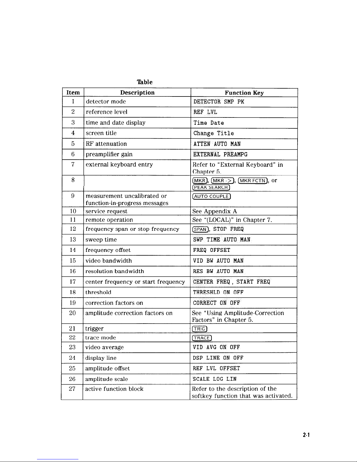
The display will be compressed slightly when using the PAL or NTSC format for the MONITOR
OUTPUT, instead of the normal format. The PAL and NTSC formats have less vertical
resolution than the spectrum analyzer display. The top and bottom of the spectrum analyzer
display are compressed slightly so that all of the information can be fit into the size required by
the MONITOR OUTPUT.

able

2-2. Screen Annotation

marker readout

Getting Started

2-l

1

‘Ihble

2-3. Screen Annotation for Trace, Trigger, and Sweep Modes

Trace Mode Trigger Mode

Sweep Mode

W = clear write (traces A/B/C)

F = free run

C = continuous

M = maximum hold (traces A/B) L = line

S

= single sweep
V = view (traces A/B/C) V = video

S

= store blank (traces A/B/C)

E = external

M = minimum hold (trace

C)

T = TV (Ootions 101 and 102 onlv)

Menu and Softkey Overview

The keys labeled FREQUENCY, CAL, and MKR are all examples of front-panel keys. Pressing
most front-panel keys accesses menus of functions that are displayed along the right side of the
display. These menus are called

softkey

menus.

Softkey

menus list functions other than those accessed directly by the front-panel keys. To

activate a function on the

softkey

menu, press the unlabeled key immediately to the right of
the annotation on the screen. The unlabeled keys next to the annotation on the display screen
are called softkeys.

Front-panel keys are designated with a box around the key label, for example,

C-1;

softkeys

are designated by shading on the key label, for example, REF LVL . The

softkeys

that

are displayed depend on which front-panel key is pressed and which menu level is enabled.
If a

softkey

function’s value can be changed, it is called an active function. The function label

of the active function appears in inverse video. For example, press

(AMPLITUDE].

This calls up

the

softkey

menu of related amplitude functions. Note the function labeled REF LVL appears
in inverse video. REF LVL also appears in the active function block, indicating that it is the
active amplitude function and can now be changed using any of the data entry controls.

A

softkey

with ON and OFF in its label can be used to turn the softkey’s function on or off. To

turn the function on, press the

softkey

so that ON is underlined. To turn the function off, press

the

softkey

so that OFF is underlined. The following example demonstrates how an ON or OFF

softkey

function will be annotated: VID AVG ON OFF (ON).

A function with AUTO and MAN in the label can either be auto-coupled or have its value
manually changed. The function’s value can be changed manually by pressing the

softkey

until MAN is underlined, and then changing its value with the numeric keypad, knob, or
step keys. To auto-couple a function, press the

softkey

so that AUTO is underlined. The

following example demonstrates how an AUTO or MAN

softkey

function will be annotated:

ATTEN

AUTO MAN (AUTO).

A summary of all front-panel keys and their related

softkeys

can be found in Chapter 8, “Key

Menus”.

2-12 Getting Started

Making a Measurement

Caution

Do not exceed the maximum input power.
The maximum input power for the HP 8590L and HP 85913 is

+30 dBm

(1 watt) continuous, 25 Vdc (with 10 dB or more attenuation).
The maximum input power for the HP

85921,

and HP 85933 is

+30 dBm

(1 watt) continuous, 0 Vdc (with input attenuation of 10 dB or more in

bands 1 through 4.)

The maximum input power for the HP 85943, HP

8594L,

HP 85953, or

HP 85963 is

+30

dBm (1 watt) continuous and 50 Vdc (ac-coupled) or 0 Vdc

(de-coupled). The input attenuation must be 10 dB or more.

Let’s begin using the spectrum analyzer by measuring an input signal. Since the 300 MHz
calibration signal (CAL OUT) is readily available, we will use it as our input signal.

You cannot hurt the spectrum analyzer by using the calibration signal and pressing any
of the keys described in this section. Don’t be afraid to play with the knob, step keys, or
number/units keypad. (If you have experimented with other keys and wish to return to a
known state, press the green

CPREsET)

key.)

1. First, turn the instrument on by pressing

ILINE).

Wait for the power-up process to complete.

2. Press the green [PRESET) key.

3. Connect the spectrum analyzer CAL

OTJT

to the INPUT

5OQ

with an appropriate cable.

4. Set the frequency.

Press the

[FREQUENCY)

key. CENTER appears on the left side of the screen, indicating that

the center-frequency function is active. The CENTER FREQ

softkey

label appears in inverse
video to indicate that center frequency is the active function. The active function block is
the space on the screen within the graticule where the center frequency messages appear.

Functions appearing in this block are active: their values can be changed with the knob,
step keys, or number/units keypad. Set the center frequency to 300 MHz with the DATA
keys by pressing 300 (MHz. The knob and step keys can also be used to set the center

frequency.

5. Set the span.
Press

(SPAN_).

SPAN is now displayed in the active function block, and the SPAN

softkey

label

appears in inverse video to indicate it is the active function. Reduce the span to 20 MHz by

using the knob, pressing the down key

(a),

or pressing 20

m.

6. Set the amplitude.

When the peak of a signal does not appear on the screen, it may be necessary to adjust
the amplitude level on the screen. Press

[AMPLITUDE).

REF LEVEL .O

dBm

appears in the

active function block. The REF LVL

softkey

label appears in inverse video to indicate

that reference level is the active function. The reference level is the top graticule line on
the display and is set to 0.0 dBm. Changing the value of the reference level changes the
amplitude level of the top graticule line.

If desired, use the reference level function to place the signal peak on the screen using the
knob, step keys, or number/units keypad. (Marker functions determine the frequency and
amplitude of a signal.)

Getting Started 2-13

Figure 2-5 demonstrates the relationship between center frequency and reference level. The
box in the figure represents the spectrum analyzer screen. Changing the center frequency
changes the horizontal placement of the signal on the screen. Changing the reference level
changes the vertical placement of the signal on the screen. Increasing the span increases the
frequency range that appears horizontally on the screen.

Note

Spectrum analyzers with Option 001 or 011 display the amplitude values in

dBmV.

Options 001 and 011 are available only for an HP

85901,

or HP 8591E.

v

f-U

REFERENCE

~FREWENC Y

LEVEL

t

AMP1 I ii/DE

c

Figure 2-5. Relationship between Frequency and Amplitude

7. Set the marker.

You can place a diamond-shaped marker on the signal peak to find the signal’s frequency
and amplitude.

To activate a marker, press the

m

key (located in the MARKER section of the front

panel). The MARKER NORMAL label appears in inverse video to show that the marker is the
active function. Turn the knob to place the marker at the signal peak.

You can also use the

[PEAK SEARCH]

key, which automatically places a marker at the highest

point on the trace.
Readouts of marker amplitude and frequency appear in the active function block and in the

upper-right corner of the display. Look at the marker readout to determine the amplitude of
the signal.

If another function is activated, the frequency and amplitude can still be identified by
looking at the marker readout in the upper-right corner of the screen.

2-14 Getting Started

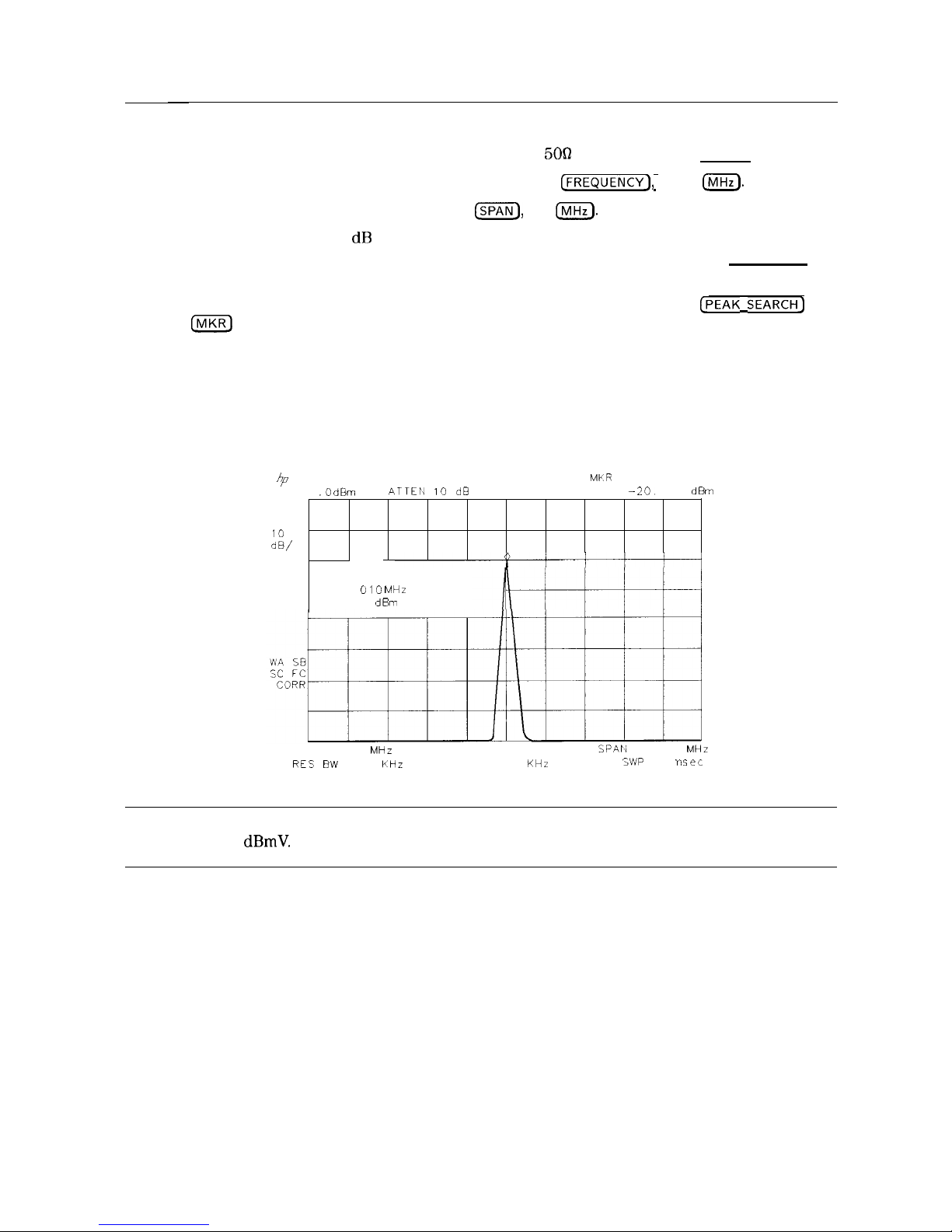
Measurement Summary

1. Connect the spectrum analyzer CAL OUT to the INPUT

5OQ

and press the (PRESET_) key.

2. Set the center frequency by pressing the following keys:

[FREQUENCY),

300

CMHz).

3. Set the span by pressing the following keys:

ISPAN),

20

m.

4. The calibration signal is 20 dB (two graticule divisions) below the top of the screen using
these spectrum analyzer settings. If desired, adjust the reference level: press [AMPLITUDE) to
activate the reference level, and use the knob or step keys to change the reference level.

5. Determine the amplitude and frequency of the signal. You can either press

[PEAK SEARCH]

or

press

m

and move the marker to the signal peak. Read the amplitude and frequency.
The display screen should look like the one in Figure 2-6. Frequency is displayed
horizontally, and amplitude (power) is displayed vertically.

‘tf

MKR

300.010 MHz

HEF .O

d6m

ATTEIJ 10 dB

--20.

17

dBm

PEAK
LOG

IO

dB/

MARKER

300

010 MHz

-20 17

dBm

CENTER 300.000

MHz

SPAll

2 000

MHz

RES

BW

10

KHz

VBW 10

KHz

5WP

co

r

nsec

Figure 2-6. Reading the Amplitude and Frequency

Note

Spectrum analyzers with Option 001 or 011 display the amplitude values in

dBmV.

Options 001 and 011 are available only for an HP 859OL or HP 85913.

Getting Started 2-15

Improving Accuracy with Self-Calibration Routines

Data from the self-calibration routine is necessary for spectrum analyzer operation. Executing
the self-calibration routine regularly ensures that the spectrum analyzer is using current
calibration data that improves the spectrum analyzer frequency and amplitude accuracy. Press
the

ICAL)

key to view the self-calibration routine menus. The last

softkey

on this menu, labeled

More 1 of 4 , provides access to additional self-calibration functions. For more detailed

information on the self-calibration softkeys, refer to Chapter 7.
The self-calibration routines add correction factors to internal circuitry. The addition of the

correction factors is required to meet frequency and amplitude specifications.
When the correction factors are added to internal circuitry, CORR (corrected) appears on the left

side of the screen.

Warm-Up Time

In order for the spectrum analyzer to meet its specifications, allow the spectrum analyzer
to warm up for 30 minutes after being turned on before attempting to make any calibrated
measurements. Be sure to calibrate the spectrum analyzer only

after

it has met operating

temperature conditions.

The spectrum analyzer frequency and amplitude self-calibration routines are initiated by the

CAL FREQ L AMPTD

softkey

in the menu located under the

ICAL]

key.

1. To calibrate the instrument, connect the spectrum analyzer CAL OUT to the INPUT

5On

connector with an appropriate cable.

Note

A low-loss cable should be used for accurate calibration. Use the

500

cable

shipped with the spectrum analyzer. (Instruments equipped with Option 001 or

011

only: use the 750 cable shipped with the spectrum analyzer).

2. On the spectrum analyzer, press (CAL) and CAL FREQ & AMPTD . Cal signal not found will
be displayed if CAL OUT is not connected to the spectrum analyzer input. The frequency
and amplitude self-calibration functions take approximately 5 minutes to finish (9 minutes
with Option

130),

at which time the internal adjustment data is in working RAM.

3. To save this data in the area of spectrum analyzer memory that is saved when the spectrum

analyzer is turned off, press CAL STORE .

Note

To interrupt the calibration routines started by CAL FREQ , CAL AMPTD , or

CAL FREQ & AMPTD , press

(-1,

(CAL), More 1 of 4 , and CAL FETCH.

CAL FETCH retrieves the previous correction factors. Improperly interrupting

the self-calibration routines may result in corrupt correction factors. (If this
occurs, press CAL FREQ t AMPTD to rerun the frequency and amplitude

self-calibration routines.)

The frequency and amplitude self-calibration functions can be done separately by using the

CAL FREQ or CAL AMPTD

softkeys

instead of CAL FREQ & AMPTD .

2-16 Getting Started

Note

If the frequency calibration CAL

FREQ

and the amplitude calibration

CAL AMPTD self-calibration routines are used, the frequency calibration should
be performed before the amplitude calibration, unless the frequency data is
known to be accurate.

The CAL

FREQ softkey

starts the frequency self-calibration routine. This routine adjusts the

frequency, sweep time, and span accuracy in approximately 2 minutes.
The CAL AMPTD

softkey

starts the amplitude calibration routine. This routine takes

approximately 3 minutes (7 minutes with Option 130) to adjust the bandwidths, log and linear
switching, IF gains, IF frequency centering, RF attenuation, and log amplifier. When the
amplitude calibration routine has finished, the preset display returns and CAL DONE is displayed.

Although the spectrum analyzer stores the correction factors in battery-backed RAM, the
data will not be saved when the spectrum analyzer power is turned off unless the data has

been stored with CAL STORE . Using CAL

STURE

stores the correction factors in an area
of spectrum analyzer memory that is accessed when the spectrum analyzer is turned on.
After the frequency and amplitude self-calibration routines are complete, CORR (corrected)

now appears on the left side of the screen, indicating that the spectrum analyzer is using its

frequency and amplitude correction factors. Correction factors can be turned off by pressing

CORRECT ON OFF . When OFF is underlined, most amplitude correction factors and some

frequency correction factors are not used.
If the self-calibration routines cannot be performed, see “Check the Basics” in Chapter 9.

Performing the Tracking Generator Self-Calibration Routine

(Option 010 or 011 only)

In order for the tracking generator to meet its specifications, allow the spectrum analyzer
to warm up for 30 minutes after being turned on before attempting to make any calibrated
measurements. Be sure to calibrate the spectrum analyzer and the tracking generator only

a&r

the spectrum analyzer has met operating temperature conditions.

Note

Since the tracking-generator self-calibration routine uses the absolute
amplitude level of the spectrum analyzer, the spectrum analyzer amplitude

should be calibrated prior to using CAL TRK GEM .

1. To calibrate the tracking generator, connect the tracking generator output (RF OUT 500) to

the spectrum analyzer INPUT

5OQ

connector, using an appropriate cable and adapters.

Note

A low-loss cable should be used for accurate calibration. Use the

5Ofl

cable

shipped with the spectrum analyzer.

(fir

Option 001 or

012:

use the 750 cable

shipped with the spectrum analyzer).

2. Press the following spectrum analyzer keys:

m),

More 1 of 4, More 2 of 4, and

CAL TRK GEN . TG SIGNAL NOT FOUND will be displayed if the tracking generator output is

not connected to the spectrum analyzer input.

3. To save this calibration data in the area of spectrum analyzer memory that is saved when
the spectrum analyzer is turned off, press (CAL) then CAL STORE.

Getting Started

2-17

Performing the YTF Self-Calibration Routine

(HP

8592L,

HP 85933, HP 85953, or HP 85963 Only)

For HP

8592L,

HP 85933, HP 85953, and HP 85963 spectrum analyzers only, the YTF

self-calibration routine should be performed periodically. See “When Is Self-Calibration

Needed?” in the following section for some helpful guidelines on how often the self-calibration

routines should be performed.

1. For the HP

8592L,

HP 85933, and HP 85963 connect a low-loss cable (such as HP part
number 8120-5148) from 100 MHz COMB OUT to the spectrum analyzer input. For the
HP 8595E connect the cable from the CAL OUT to the spectrum analyzer input.

2. Press

LCAL),

then CAL YTF . The YTF self-calibration routine completes in approximately:

Model Number Calibration Time

HP 8592L

7 minutes

HP 85933

7

minutes

HP 85953

3

minutes

HP 85963

5

minutes

3. Press

a),

then CAL STORE to save the calibration factors in memory.

4. Press (PRESET) to return to normal operation.

When Is Self-Calibration Needed?

While it is difficult to provide general advice for your specific measurement needs, the
following suggestions may help you decide when to use the self-calibration features:

1. Perform the frequency and amplitude self-calibration routines whenever the instrument
experiences significant environmental changes such as temperature

(f5

“C), humidity, shock,
or vibration (such as may occur during shipping or transport). This is especially important
if the frequency and amplitude self-calibration routines were performed last in a different
environment.

2. If the environment is relatively stable (for example, a lab environment), use
CAL

FREQ &

AMPTD monthly. After being turned off overnight, the spectrum analyzer will

need to warm up, but should not require self-calibration.

3. To achieve optimal amplitude accuracy for relative measurements:
a. Keep the spectrum analyzer in a stable environment.

b. Use CAL

FREQ t

AMPTD before beginning the first measurement.

c. Keep the spectrum analyzer turned on between measurements.

d.

Do not use CAL

FREQ &

AMPTD before subsequent measurements (the amplitude drift is

normally smaller than the self-calibration uncertainty).

4. If you change the input signal for EXT REF IN, run the frequency and amplitude

self-calibration routines using CAL OUT. Amplitude calibration is required to improve IF
centering.

5. If preselector peaking (PRESEL PEAK ) has more than a 2 dB effect on the signal amplitude

when in BAND 1 or above, and in a single band sweep, then perform the YTF self-calibration
routine and store the data with CAL STORE . The YTF self-calibration routine improves the
preselector default values. (HP

8592L,

HP 85933, HP

85956

or HP

859622

only.)

2-18 Getting Started

6. If accurate self-calibration is needed temporarily in a different environment, use

CAL

FREQ t

AMPTD , but do not press CAL STORE . The temporary correction factors will be

used until the spectrum analyzer is turned off or until CAL FETCH is pressed.

Memory Card Insertion and Battery Replacement

The memory card reader is available for the HP

859OL,

HP

8592L,

and HP 8594L as Option 003.
Use the following information to ensure that the memory card is inserted correctly. Improper
insertion causes error messages to occur, but generally does not damage the card or instrument.
Care must be taken, however, not to force the card into place. The cards are easy to insert
when installed properly.

1. Locate the arrow printed on the card’s label.

2. Insert the card with its arrow matching the raised arrow on the bezel around the

card-insertion slot. See Figure 2-7.

Figure 2-7. Inserting the Memory Card

3. Press the card into the slot. When correctly inserted, about 19 mm (0.75 in) of the card is
exposed from the slot.

Getting Started

2-l

9

Changing the Memory Card Battery

It is recommended that the memory card battery be changed every 2 years. The battery is a
lithium commercial CMOS type battery, part number CR 2016 or HP part number

1420-0383.

Note

The minimum lifetime of the battery (under ordinary conditions) is more
than 2 years.

The date that the memory card battery was installed is either engraved on the side of the
memory card or written on a label on the memory card.

If the memory card does not have a label with the date that the battery was installed, use
the date code engraved on side of the memory card. The date code engraved on the memory
card consists of numbers and letters engraved in the black plastic on the side of the memory
card. See Figure 2-8. The first number indicates the year, the following two characters indicate
the month, and the following number indicates the week in the month that the memory card

battery was installed. For example,

8OC3

indicates the battery was installed in the third week

in October in 1988.

Figure 2-8. Memory Card Battery Date Code Location

2-20

Getting Started

Procedure to Change the Memory Card Battery

The battery is located beside the card’s write-protect switch on the end opposite the connector.

Caution

The battery power enables the memory card’s memory to retain data. You can

lose the data when the battery is removed. Replace the battery while the card
is installed in a powered-up instrument.

1. Locate the groove along the edge of the battery clip. See Figure 2-9.

2. Gently pry the battery clip out of the card. The battery fits within this clip.

3. Replace the battery, making sure the plus

(+)

sign on the battery is on the same side as the

plus ( + ) sign on the clip.

HP Part Number: 1420-0383 or commercial Lithium CMOS type part number CR 2016.

.

I!!!!

DO NOT THROW BATTERIES AWAY BUT
COLLECT AS SMALL CHEMICAL WASTE.

0

sk78Oa

4. Insert the battery clip into the memory card, holding the clip as oriented in Figure 2-9.
(Face the “open” edge of the clip toward the write-protect switch on the memory card.)

5. Write the date that the battery was replaced on the memory card label. This will help you
to remember when the battery should be replaced.

.

=

INSERTION END

m

HEWLETT

PACKAPD

a5700A
,?K

BYTE

HAM

WPITE PRCJTECT 5WlTCH

BATTERY

SLOT

GPOOVE

BATTEP I’ ii P

Figure 2-9. Memory Card Battery Replacement

Getting Started 2-21

Analyzer Battery Information

The HP 8590 Series spectrum analyzers use a 3.6 V lithium battery to enable the spectrum
analyzer memory to retain data. The date when the battery was installed is on a label on the
rear panel of the spectrum analyzer. See Figure

2-10.

The minimum life expectancy of the battery is 8 years at 25

“C,

or 1 year at 55

“C.

If you
experience problems with the battery or the recommended time period for battery replacement
has elapsed, see “How to Return Your Analyzer for Service” in Chapter 9.

If you wish to replace the battery yourself, you can purchase the service documentation that
provides all necessary test and maintenance information. The battery is soldered onto the
spectrum analyzer processor board.

Warning

There is a danger of explosion if the battery is incorrectly replaced.
Replace only with the same or equivalent type recommended. Discard
used batteries according to manufacture’s instructions.

DO NOT THROW BATTERIES AWAY BUT
COLLECT AS SMALL CHEMICAL WASTE.

sk780a

You can order the service documentation for an HP 8590 Series spectrum analyzer through your
HP Sales and Service office. The documentation is described under “Service Documentation

(Option 915)” in Chapter 10 of this manual.

After replacing the spectrum analyzer battery, write the date of battery replacement on the

rear-panel label.

BATTERI

LIFE

0

8 ‘YEARS

AT

‘75’C

1 r EAP AT

55’C

>

IdSTALLED

p I.1

1 3 2

e

Figure 2-10. Rear-Panel Battery Information Label

2.22

Getting Started

3

Making Basic Measurements

What You’ll Learn in This Chapter

This chapter demonstrates basic spectrum analyzer measurements with examples of typical
measurements; each measurement focuses on different functions. The measurement procedures
covered in this chapter are listed below.

n Resolving signals of equal amplitude using the resolution bandwidth function.
n Resolving small signals hidden by large signals using the resolution bandwidth function,
n Increasing the frequency readout resolution using the marker counter.

w

Decreasing the frequency span using the marker track function.

w

Peaking signal amplitude using preselector peak (HP

8592L,

HP

8593E,

HP 85953, or

HP 85963 only).

n Tracking unstable signals using marker track and the maximum hold and minimum hold

functions.

n Comparing signals using delta markers.

w

Measuring low-level signals using attenuation, video bandwidth, and video averaging.

w

Identifying distortion products using the RF attenuator and traces.

w

Using the spectrum analyzer as a receiver in zero frequency span.

w

Measuring signals near band boundaries using harmonic lock (HP

8592L,

HP

8593E,

HP 85953, or HP 8596E only).

To find descriptions of specific spectrum analyzer functions refer to Chapter 7 “Key

Descriptions”.

Making Basic Measurements 3-1

Resolving Signals of Equal Amplitude Using the Resolution
Bandwidth Function

In responding to a continuous-wave signal, a swept-tuned spectrum analyzer traces out the
shape of the spectrum analyzer intermediate frequency (IF) filters. As we change the filter
bandwidth, we change the width of the displayed response. If a wide filter is used and two
equal-amplitude input signals are close enough in frequency, then the two signals appear as
one. Thus, signal resolution is determined by the IF filters inside the spectrum analyzer.

The resolution bandwidth (RES SW) function selects an IF filter setting for a measurement.
Resolution bandwidth is defined as the 3 dB bandwidth of the filter. The 3 dB bandwidth tells
us how close together equal amplitude signals can be and still be distinguished from each other.

Generally, to resolve two signals of equal amplitude, the resolution bandwidth must be less

than or equal to the frequency separation of the two signals. If the bandwidth is equal to the

separation a dip of approximately 3 dB is seen between the peaks of the two equal signals, and
it is clear that more than one signal is present. See Figure 3-2.

In order to keep the spectrum analyzer calibrated, sweep time is automatically set to a
value that is inversely proportional to the square of the resolution bandwidth. So, if the
resolution bandwidth is reduced by a factor of 10, the sweep time is increased by a factor of

100 when sweep time and bandwidth settings are coupled. (Sweep time is proportional to

1/BW2.)

For fastest measurement times, use the widest resolution bandwidth that still permits
discrimination of all desired signals. The spectrum analyzer allows you to select from 30 Hz to
3 MHz resolution bandwidth in a 1, 3, 10 sequence, plus 5 MHz, for maximum measurement
flexibility.

Example: Resolve two signals of equal amplitude with a frequency separation of 100

kHz.

1. To obtain two signals with a 100 kHz separation, connect the calibration signal and a signal
source to the spectrum analyzer input as shown in Figure 3-l. (If available, two sources can
be used.)

Figure 3-l. Set-Up for Obtaining Two Signals

2. If you are using the 300 MHz calibration signal, set the frequency of the source 100 kHz
greater than the calibration signal (that is, 300.1 MHz). The amplitude of both signals should

be approximately -20 dBm.

3. On the spectrum analyzer, press

Cm].

Set the center frequency to 300 MHz, the span to

2 MHz, and the resolution bandwidth to 300 kHz by pressing

(FREQUENCY]

300 [$iK),

@Ei@

2

IFvlHz_),

then

Isw]

300

(kHz).

A single signal peak is visible.

3-2 Making Basic Measurements

Note

When using an HP 8590L with Option 713 or an HP 8592L with Option 713,
and the signal peak cannot be found, increase the span to 20 MHz by pressing

ISPAN)

20

INIHz_).

The signal should be visible. Press

[PEAK SEARCH], (MKRJ,

MK TRACK ON OFF (ON), then

ISPAN_)

2

INIHz)

to bring the signal to center

screen. Then press MK TRACK

Old

OFF so that OFF is underlined to turn the

marker track function off.

4. Since the resolution bandwidth must be less than or equal to the frequency separation of
the two signals, a resolution bandwidth of 100 kHz must be used. Change the resolution
bandwidth to 100 kHz by pressing

(swl

100

(kHz).

Two signals are now visible as in
Figure 3-2. Use the knob or step keys to further reduce the resolution bandwidth and better
resolve the signals.

&

REF

PEAK

LOG

10

dB/

0

dB” ATTEN

10

d8

CENTER 300 000 MHz

SPAN 2

000 MHZ

CRES BW 100

kHL

VBW

30 CHZ

SW

20

mset

Figure 3-2. Resolving Signals of Equal Amplitude

As the resolution bandwidth is decreased, resolution of the individual signals is improved and
the sweep time is increased. For fastest measurement times, use the widest possible resolution
bandwidth. Under preset conditions, the resolution bandwidth is “coupled” (or linked) to span.

Since the resolution bandwidth has been changed from the coupled value, a

“#”

mark appears
next to RES BW in the lower-left corner of the screen, indicating that the resolution bandwidth
is uncoupled. (Also see the

CAUTO COUPLE)

key description in Chapter 7.)

Note

To resolve two signals of equal amplitude with a frequency separation of
200

kHz,

the resolution bandwidth must be less than the signal separation, and
resolution of 100 kHz must be used. The next larger filter, 300 kHz, would
exceed the 200 kHz separation and would not resolve the signals.

Making Basic Measurements 3-3

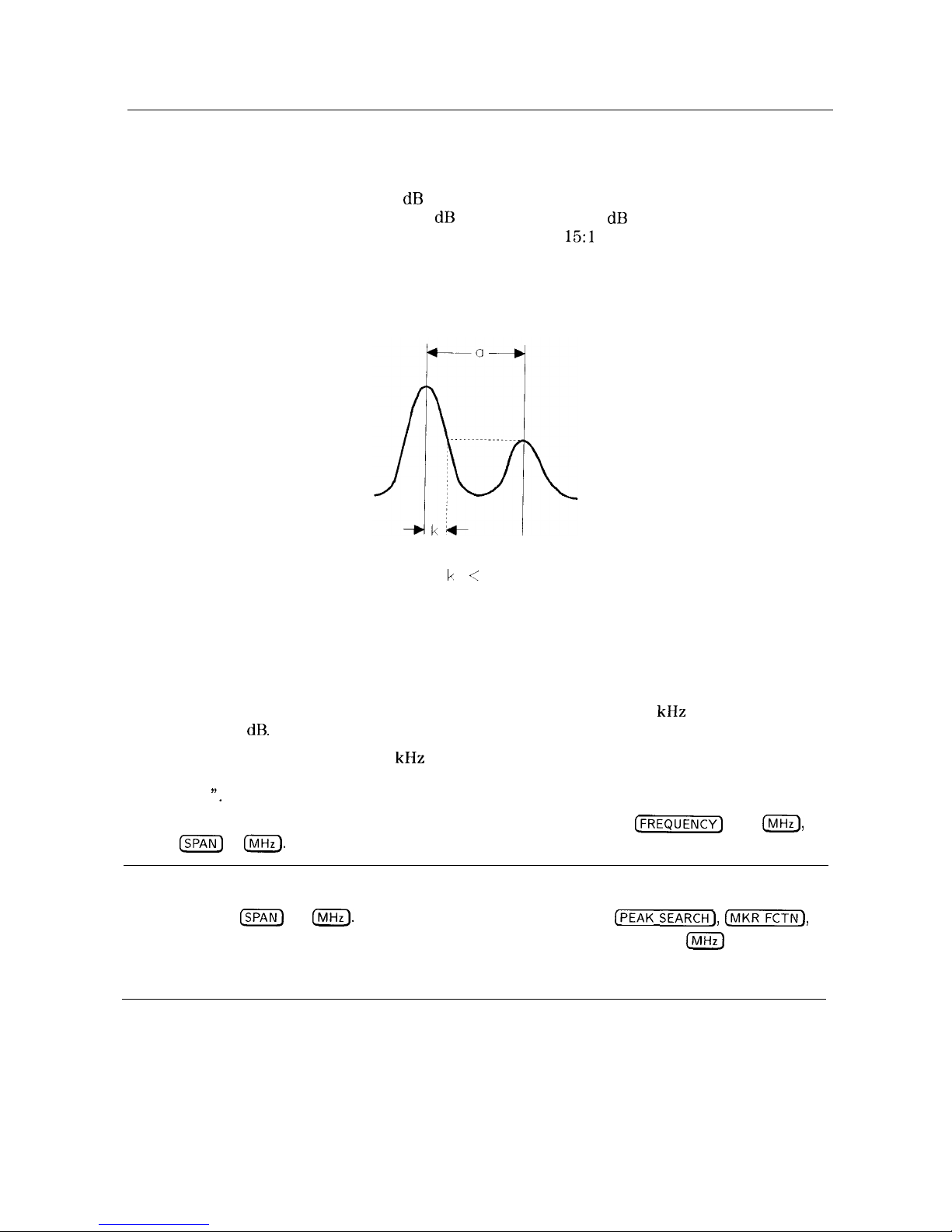
Resolving Small Signals Hidden by Large Signals Using the
Resolution Bandwidth Function

When dealing with resolution of signals that are not equal in amplitude, you must consider the
shape of the IF filter as well as its 3 dB bandwidth. The shape of the filter is defined by the
shape factor, which is the ratio of the 60 dB bandwidth to the 3 dB bandwidth. (Generally,
the IF filters in this spectrum analyzer have shape factors of 15:l or less.) If a small signal is
too close to a larger signal, the smaller signal can be hidden by the skirt of the larger signal. To
view the smaller signal, you must select a resolution bandwidth such that k is less than a.
See Figure 3-3.

k <

a

Figure 3-3. Resolution Bandwidth Requirements for Resolving Small Signals

The separation between the two signals must be greater than half the filter width of the larger
signal at the amplitude level of the smaller signal.

Example: Resolve two input signals with a frequency separation of 200 kHz and an amplitude
separation of 60

dB.

1. To obtain two signals with a 200 kHz separation, connect the equipment as shown in the
previous section, “Resolving Signals of Equal Amplitude Using the Resolution Bandwidth
Function

“.

2. Set the center frequency to 300 MHz and the span to 2 MHz: press

k-1

300

m,

then

ISPAN)

2

IIVIHz).

Note

When using an HP 8590L with Option 713 or an HP 8592L with Option 713,
and the signal peak cannot be found, increase the span to 20 MHz by pressing

ISPAN)

20

INIHz).

The signal should be visible. Press

[PEAK

SEARCH],

(rvlKR),

MK TRACK ON OFF so that ON is underlined. Then (SPAN) 2

INIHz)

to bring the

signal to center screen. Then press MK TRACK ON OFF to OFF to turn the
marker track function off.

3-4 Making Basic Measurements

3. Set the source to 300.2 MHz, so that the signal is 200 kHz higher than the calibration signal.
Set the amplitude of the signal to -80 dBm (60 dB below the calibration signal).

4. Set the 300 MHz signal to the reference level by pressing

[PEAK SEARCH),

[MKR),

then

MARKER -+REF LVL .

If a 10 kHz filter with a typical shape factor of 15: 1 is used, the filter will have a bandwidth
of 150 kHz at the 60 dB point. The half-bandwidth (75

kHz)

is narrower than the frequency

separation, so the input signals will be resolved.

4-J

MKR

300.010 MHz

REF

-23

7

dBrn AaTTEN

10

dB

0

-23 86

dBm

PEAK
LOG

10

dB/

MARKER

300.010 MHz

-23.86 dBm

CENTER 300 000

MHZ

SP,%hl

2

000

MHZ

RES EW 10

kHZ

YBW

10

kHZ

SW 60

msec

Figure 3-4. Signal Resolution with a 10

kHz

Resolution Bandwidth

If a 30 kHz filter is used, the 60 dB bandwidth will be 450 kHz. Since the half-bandwidth
(225

kHz)

is wider than the frequency separation, the signals most likely will not be resolved.
See Figure 3-5. (To determine resolution capability for intermediate values of amplitude level
differences, consider the filter skirts between the 3 dB and 60 dB points to be approximately
straight. In this case, we simply used the 60 dB value.)

4

MKR

300

010 MHz

REF

-23

7

dBm

ATTEN

10

dB

0

-23 87

dBm
PEPK

LOG

In

,1!

I

IW

dB/

i \

.-

RES EW

30

kHZ

\

CENTER

3Ub3.000

MHz

SPAN 2

000 MHz

#RES BW 38

kHL “BW

30

kHL

SW20msec

Figure 3-5. Signal Resolution with a 30

kHz

Resolution Bandwidth

Making Basic Measurements 3-5

Increasing the Frequency Readout Resolution Using the Marker

Counter

Note

This application cannot be performed using an HP

8590L

with Option 713 or an

HP 8592L with Option 713.

The marker counter increases the resolution and accuracy of frequency readout. When using

the marker count function, if the bandwidth to span ratio is too small (less than O.Ol), the
Reduce Span message appears on the display. If Widen RES BW is displayed, it indicates that the
resolution bandwidth is too narrow. Resolution bandwidths less than 300 Hz are not allowed if
you are using firmware with a revision date prior to 930506. If the signal being counted is the
largest signal within the 300 Hz bandwidth then the count will be correct. If there is another,
larger signal (even off the display), the count will be for the larger signal.

Example: Increase the resolution and accuracy of the frequency readout on the signal of
interest.

1.

2.

3.

4.

Place a marker on the signal of interest. (If you are using the CAL OUT signal, place the
marker on the 300 MHz calibration signal. Press

[FREQUENCY]

300

IIVIHz), (SPAN]

100

m),

and

(PEAK SEARCH].)

Press

(mFCTN),

then MK COUNT ON OFF (ON should be underlined) to turn the marker
counter on. COUNTER and the frequency and amplitude of the marker will appear in the
active function area.

Increase the counter resolution by pressing More 1 of 2 , CNT RES AUTO MAN and then
entering the desired resolution using the step keys or the number/units keypad. For
example, press 1

m.

The marker counter readout is in the upper-right corner of the

screen. The resolution can be set from 10 Hz to 100

kHz.

The marker counter remains on until turned off. Turn off the marker counter by pressing

(FCTNJ

then MK COUNT ON OFF (until OFF is underlined). (MARKER ALL OFF also turns

the marker counter off.)

43

CNTRCNTR 300 000300 000

MHzMHz

REF 0

d&r

REF 0

d&r

!iTTEld!iTTEld

1010

dBdB

-20 05-20 05dBrndBrn

PEAKPEAK

LOG

10

rlB/

Figure 3-6. Using the Marker Counter

3-6 Making Basic Measurements

Decreasing the Frequency Span Using the Marker Track
Function

Using the spectrum analyzer marker track function, you can quickly decrease the span while
keeping the signal at center frequency.

Example: Examine a carrier signal in a 200 kHz span.

1. Press (PRESET], tune to a carrier signal, and place a marker at the peak. (If you are using the
CAL OUT signal, place the marker on the 300 MHz calibration signal. Press

C-1,

300

m, ISPAN),

200

IMHz),

and

[PEAK SEARCH).)

Press

@iGX%],

MK TRACK ON OFF (ON) and the signal will move to the center of the

screen, if it is not already positioned there (note that the marker must be on the signal).

Because the marker track function automatically maintains the signal at the center of the

screen, you can reduce the span quickly for a closer look. If the signal drifts off of the
screen as you decrease the span, use a wider frequency span.

Press (SPAN), 200

IkHz).

The span decreases in steps as automatic zoom is completed.

See Figure 3-7. You can also use the knob or step keys to decrease the span or use the

PEAK ZOOM function under

ISPAN).

Press MK TRACK ON OFF again so that (OFF) is underlined to turn off the marker track
function.

Note

When you are finished with the example, turn off the marker tracking function.

b

MkR-TRK

300.0010 MHZ

REF

0

dB”

ATTEN

10 dB

-20

04 d0rn

CINTER 300

0015 MHZ SPAN 200.0 kHZ

RE5 tlW

3 ~HL

'VBW3kHz

CWP

100

msec

Figure 3-7. After Zooming In on the Signal

Making Basic Measurements 3-7

Peaking Signal Amplitude with Preselector Peak

Note

This application should only be performed using an HP

8592L,

HP

8593E,

HP 8595E, or HP 85963.

PRESEL PEAK works above 2.9

GHz

only (bands 1 through 4).

The preselector peak function automatically adjusts the preselector tracking to peak the
signal at the active marker. Using preselector peak prior to measuring a signal yields the most
accurate amplitude reading at the specified frequency. To maximize the peak response of
the preselector and adjust the tracking, tune the marker to a signal and press [AMPLITUDE),

PRESEL PEAK .

Note

PRESEL PEAK maximizes the peak response of the signal of interest, but may

degrade the frequency response at other frequencies. Use PRESEL DEFAULT or

[PRESET]

to clear preselector-peak values before measuring a signal at another

frequency.

PRESEL DEFAULT provides the best flatness for a full single-band, for viewing

several signals simultaneously.

Example: Use the knob, step keys, or

[PEAK SEARCH]

to place the marker on your signal and

then press

CAMPLITUDE)

and PRESEL PEAK . The message CAL : PEAKING appears in the active

function block while the routine is working.

b

MKR

18

005

GHT

REF 0

dBm

ATTEN

10

d0

-41 R> dR

m

PEAK
LOG

10

/

CENTER

18.000

GHz

SPAN

2

000

GH,

HE5 BW 3

MHz

VBW

1

MHz

SWP

40

msec

Figure 3-8. Peaking Signal Amplitude Using Preselector Peak

3-8 Making Basic Measurements

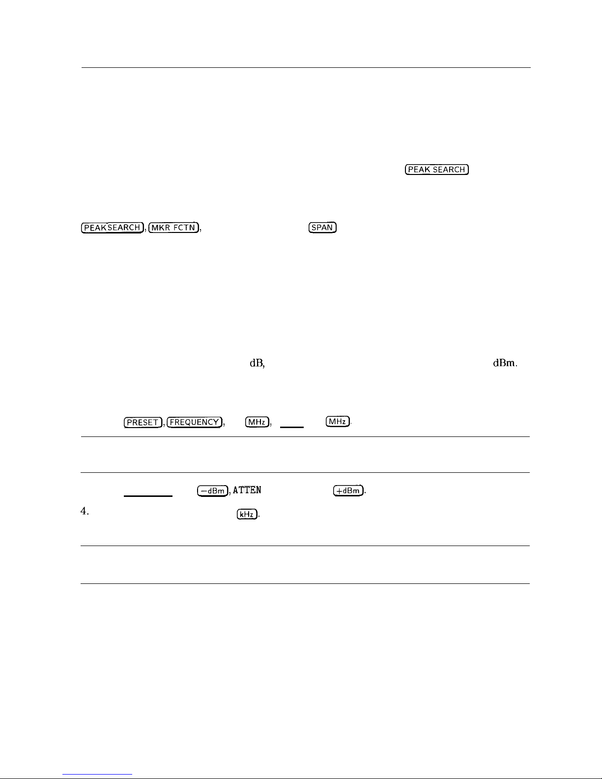
Tracking Unstable Signals Using Marker Track and the
Maximum Hold and Minimum Hold Functions

The marker track function is useful for tracking unstable signals that drift with time. The
maximum hold and minimum hold functions are useful for displaying modulated signals which
appear unstable, but have an envelope that contains the information-bearing portion of the
signal.

MK TRACK ON OFF may be used to track these unstable signals. Use

[PEAK SEARCH]

to place a

marker on the highest signal on the display. Pressing MK TRACK ON OFF (ON) will bring that
signal to the center frequency of the graticule and adjust the center frequency every sweep

to bring the selected signal back to the center. SPAN ZOOM is a quick way to perform the

IPEAK SEARCH],

C-1,

MK TRACK ON OFF ,

m

key sequence.

Note that the primary function of the marker track function is to track unstable signals, not to
track a signal as the center frequency of the spectrum analyzer is changed. If you choose to
use the marker track function when changing center frequency, check to ensure that the signal
found by the tracking function is the correct signal.

Example: Use the marker track function to keep a drifting signal at the center of the display
and monitor its change.

This example requires a modulated signal. An acceptable signal can be easily found by

connecting an antenna to the spectrum analyzer input and tuning to the FM broadcast band
(88 to 108 MHz). Set the spectrum analyzer center frequency for 100 MHz with a span of
20 MHz, an attenuator setting of 0

dB,

and reference level setting of approximately -40 dBm.

Your circumstances may be slightly different, depending on building shielding and proximity to
transmitters.

1. Connect an antenna to the spectrum analyzer input.

2. Press

cm),

[FREQUENCY],

100

IIVIHz),

(SPAN], 20

INIHz_).

Note

Use a different signal frequency if no signal is available at 100 MHz in your
area.

3. Press (AMPLITUDE], 40

C-dBm), ATTEN

AUTO MAN , 0

(+dBm].

4.

Press (SPAN), SPAN ZOOM, 500

(kHz).

Notice that the signal has been held in the center of the display.

Note

If the signal you selected drifts too quickly for the spectrum analyzer to keep
up with, use a wider span.

Making Basic Measurements 3-9

5.

The signal frequency drift can be read from the screen if both the marker track and marker
delta functions are active. Press

INIKR),

MARKER A ,

Cm),

MK TRACK ON OFF ; the
marker readout indicates the change in frequency and amplitude as the signal drifts. See
Figure 3-9.

b

MKR A-TRII 28.8 ktiz

REF -40 0

dBm

#ATTEN 0

dB

-

05 dB

PEAK

LOG

0

10

I

d

dB/

1

k/Afi: I

CENTER 104 9275

MHZ

RES ew 10

CHZ

SPAN 500.0

I-Hz

“BW10kHZ

SWP

30

m5ec

Figure 3-9. Using Marker Tracking to Track an Unstable Signal

The spectrum analyzer can measure the short- and long-term stability of a source. The

maximum amplitude level and the frequency drift of an input signal trace can be displayed and
held by using the maximum-hold function. The minimum amplitude level can be displayed by
using minimum hold (available for trace C only).

You can use the maximum-hold and minimum-hold functions if, for example, you want to
determine how much of the frequency spectrum an FM signal occupies.

Example: Using the maximum-hold and minimum hold functions, monitor the envelopes of a
signal.

1. Connect an antenna to the spectrum analyzer input.

2. Press

CPRESET_), [FREQUENCY],

100

m,

and

m,

20

IMHz).

3.

Press

[AMPLITUDE_),

40

I-),

ATTEN

AUTO MAN , 0

(+dBm), m),

SPAN ZOOM , 500

@.

Notice that the signal has been held in the center of the display.

4. Turn off the marker track function by pressing MK TRACK ON OFF (OFF).,

5.

To measure the excursion of the signal, press [TRACE) then MAX HOLD A . As the signal

varies, maximum hold maintains the maximum responses of the input signal, as shown in
Figure 3- 10.

3.10 Making Basic Measurements

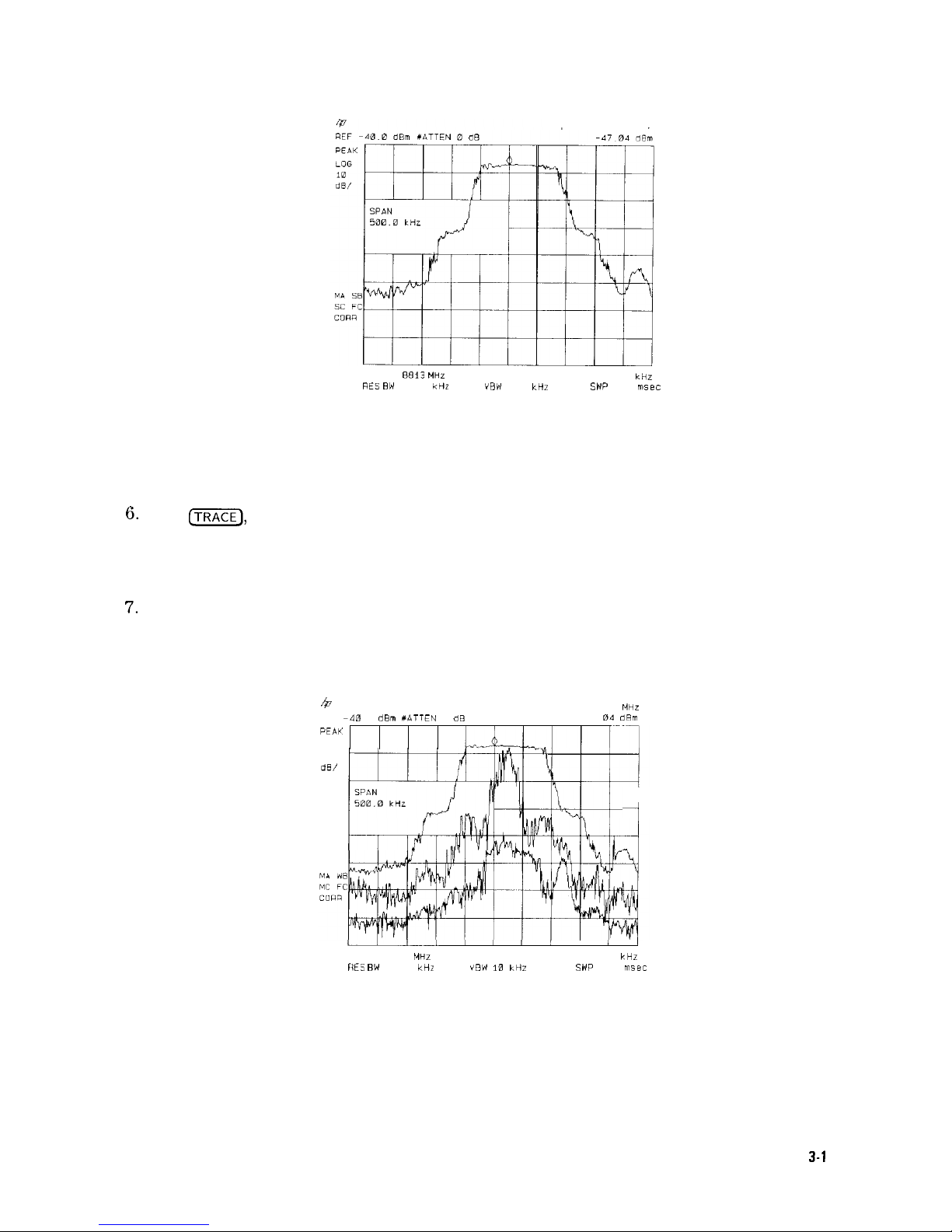
CENTER 104

8813

MHz

MKR 104.8813 MHz

SPAN 500.0

kHz

RES BW 10

ktiz

VEW

10 kHZ

SWP

30

msec

Figure 3-10. Viewing an Unstable Signal Using Max Hold A

Annotation on the left side of the screen indicates the trace mode. For example, MA SB SC
indicates trace A is in maximum-hold mode, trace B and trace C are in store-blank mode.
See “Screen Annotation” in Chapter 2.

6.

Press

(j%?Fj,

TRACE A B C to select trace B. (Trace B is selected when B is underlined.)

Press CLEAR WRITE B to place trace B in clear-write mode, which displays the current

measurement results as it sweeps. Trace A remains in maximum-hold mode, showing the
frequency shift of the signal.

7.

Press TRACE A B C to select trace C (C should be underlined). Press MIN HOLD C . Trace C

is in the minimum-hold mode and displays the minimum amplitude of the frequency drift of
the signal.

b

MKR 104.8813

MHZ

REF

-400d&n XATTEN0dB

-4704dRm

PE,4II

LOG

10

dE/

i

I

CENTER 104 8813 MHz

SPAN 500.0

kHr

fiES BW

10 CHZ

VOW

10

kHr

SWP

30

msec

Figure 3-11. Viewing an Unstable Signal With Max Hold, Clear

Write, and Min Hold

Making Basic Measurements

3-l

1

Comparing Signals Using Delta Markers

Using the spectrum analyzer, you can easily compare frequency and amplitude differences
between signals, such as radio or television signal spectra. The spectrum analyzer delta marker
function lets you compare two signals when both appear on the screen at one time or when
only one appears on the screen.

Example: Measure the differences between two signals on the same display screen.

1. Connect the spectrum analyzer CAL OUT to the INPUT

50R.

Press @ZZY’). For the

HP 85933 only, set the center frequency to 900 MHz and the span to 1.8

GHz:

press

[FREQUENCY],

900

($iiC),

(SPANS, 1.8

IGHz).

The calibration signal and its harmonics appear on the display.

2.

Press

(PEAK SEARCH]

to place a marker at the highest peak on the display. The

NEXT PK RIGHT and NEXT PK LEFT

softkeys

move the marker from peak to peak. Press

NEXT PK RIGHT to move the marker to the 300 MHz calibration signal. See Figure 3-12.

The signal that appears at the left edge of the screen is the spectrum analyzer local
oscillator (LO) and represents 0 Hz.

4

MKR 311

MHz

REF

0

dBm

ATTEN

IB

dB

-20 15

dBm

PEAK
LOG

10

dB/

n

u/-.

J

CEFITER

900 MHZ

SPaN

1

A00

GHZ

RES BW 3

MHZ VBW

1 MHz

SWP

20 msec

3-12. Placing a Marker on the CAL OUTFigure

Signal

3. Press MARKER A to activate a second marker at the position of the first marker. Move the
second marker to another signal peak using the NEXT PK RIGHT or NEXT PK LEFT

softkeys

or the knob.

4. The amplitude and frequency difference between the markers is displayed in the active
function block and in the upper-right corner of the screen. See Figure 3-13.

Press

(MKR),

More 1 of 2 , then MARKER ALL OFF to turn the markers off.

3-12 Making Basic Measurements

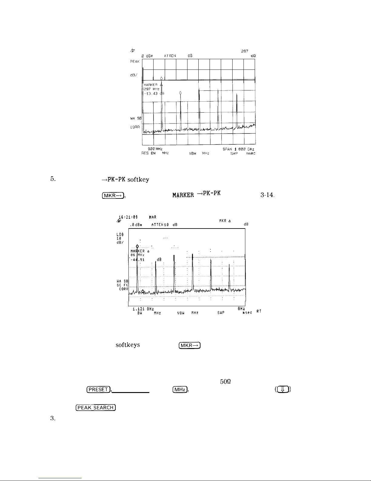
MKA A

2!97

MHz

4

REF

PEaK

LOG

10

dB/

0 dEm

ATTEN

10

dB

-13.43 dB

WA SB

SC FC

COAR

CENTER

900

MHz

SPQN

1

600

GH.?

RES EW 3

MHZ

VBW1MHZ

SWP20msec

Figure 3-13. Using the Marker Delta Function

5.

The MARKER

-+PK-PK softkey

can be used to find and display the frequency and amplitude
difference between the highest- and lowest-amplitude signals. To use this automatic
function, press

(MKR--t),

More 1 of 2 ,

M&RKER -+PK-PK

. See Figure

3-14.

16:21:03

12

MhR 1992

&

NKR A 86 MHz

REF .B

dBm

RTTEN

18

dB

-44.91 dB

PEAK I

I

LOG

18

dB/

:

."'

'.

.'.

I

'I'

:

"

I'":&

d8

1

,,,.. 1 .,.,,,,,I..,,,;

,,,,,,..,,,,,,,...,,,.,......

1

CENTER I.121 GHz

SPAN 1.919 GHz

RES 8W 3.8 NHz

UBW

1 NHz

SWP 38.4

nts.ee RT

Figure 3-14. Using the Marker to Peak/Peak Function

The frequency and amplitude differences between the signals appear in the active function
block. In addition, the

softkeys

accessed by

(s)

appear on the screen.

Example: Measure the frequency and amplitude difference between two signals that do not
appear on the screen at one time. (This technique is useful for harmonic distortion tests when
narrow span and narrow bandwidth are necessary to measure the low-level harmonics.)

1. Connect the spectrum analyzer CAL OUT to the INPUT

5OQ

(if you have not already done

so). Press

[PREsETI,

(FREQUENCY), 300

m,

(SPAN) and the step down key

(a)

to narrow

the frequency span until only one signal appears on the screen.

2. Press

(PEAK SEARCH)

to place a marker on the peak.

3.

Press MARKER A to identify the position of the first marker.

Making Basic Measurements 3-13

4. Press CFREQUENCY] to activate center frequency. Turn the knob clockwise slowly to adjust

the center frequency until a second signal peak is placed at the position of the second
marker. It may be necessary to pause occasionally while turning the knob to allow a sweep
to update the trace. The first marker remains on the screen at the amplitude of the first
signal peak.

Note

Changing the reference level changes the marker delta amplitude readout.

The annotation in the upper-right corner of the screen indicates the amplitude and frequency
difference between the two markers. See Figure 3-15.

To turn the markers off, press

IIVIKR),

More 1 of 2 , then MARKER ALL OFF .

~ - ““7

3

h

MKR A 306.~ ,mn

REF 0

dBm

ATTEN

10

dB

-13

33 dL

PEAK
LOG

10

d8/

CEIlTER

597 5 MHz

SPAN 500.0

MHz

RES EW 3 MHZ

VEW

1

MHZ

SWP 28

msec

Figure 3-15. Frequency and Amplitude Difference between Signals

3-14 Making Basic Measurements

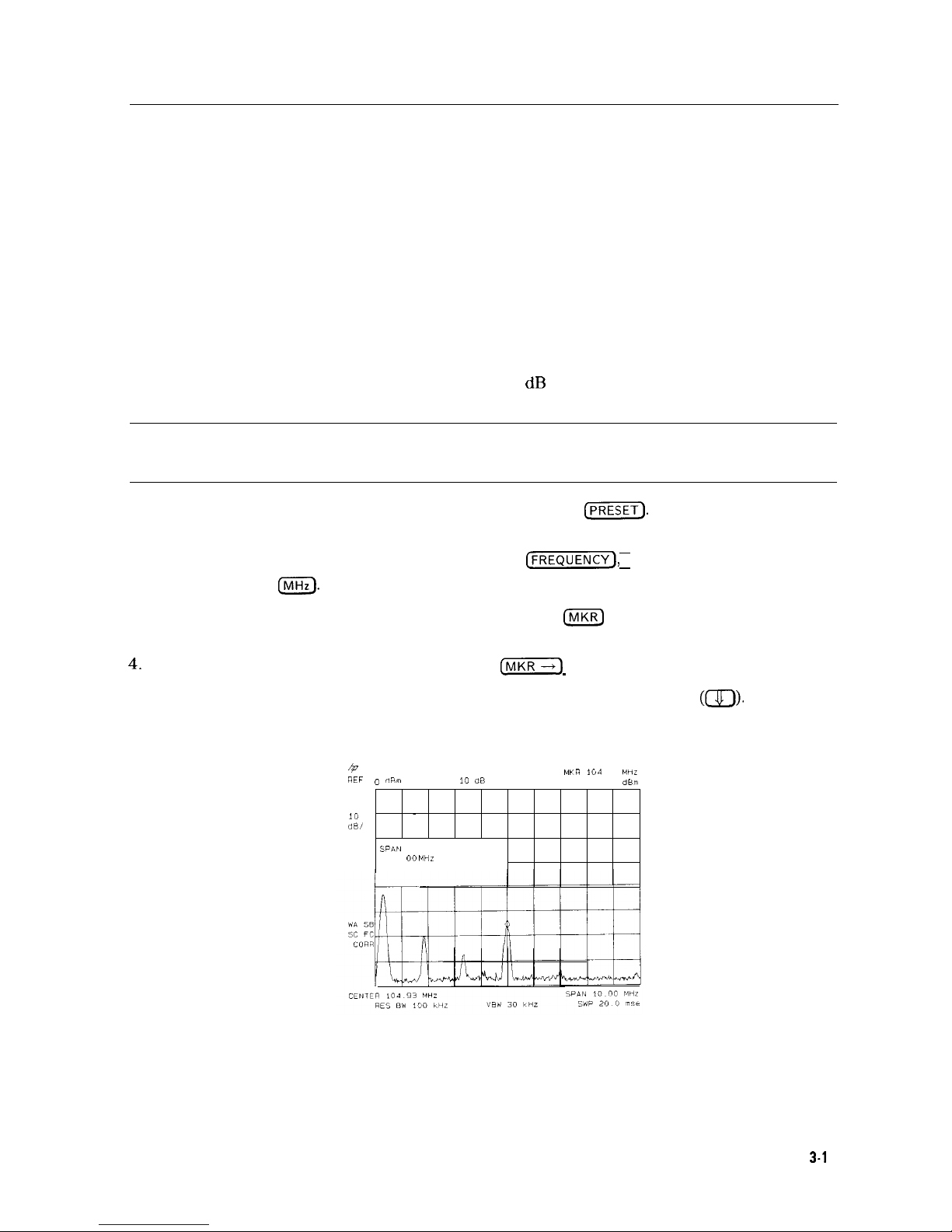
Measuring Low-Level Signals Using Attenuation, Video
Bandwidth, and Video Averaging

Spectrum analyzer sensitivity is the ability to measure low-level signals. It is limited by the
noise generated inside the spectrum analyzer. The spectrum analyzer input attenuator and

bandwidth settings affect the sensitivity by changing the signal-to-noise ratio. The attenuator

affects the level of a signal passing through the instrument, whereas the bandwidth affects the
level of internal noise without affecting the signal. In the first two examples in this section, the
attenuator and bandwidth settings are adjusted to view low-level signals.

If, after adjusting the attenuation and resolution bandwidth, a signal is still near the noise,
visibility can be improved by using the video-bandwidth and video-averaging functions, as
demonstrated in the third and fourth examples.

Example: If a signal is very close to the noise floor, reducing input attenuation brings the

signal out of the noise. Reducing the attenuation to 0 dB maximizes signal power in the

spectrum analyzer.

Note

The total power of all input signals at the spectrum analyzer input must not
exceed the maximum power level for the spectrum analyzer.

1. Connect an antenna to the spectrum analyzer input. Press

Cm).

2. Reduce the frequency range to view a low-level signal of interest. For example, narrow the
frequency span from 88 MHz to 108 MHz by pressing

[FREQUENCY],

START FREQ , 88 (MHz),

STOP FREQ , 108

IRnHz).

3. Place a marker on the low-level signal of interest. Press

(MKR)

and use the knob to position

the marker at the signal’s peak.

4.

Place the signal at center frequency by pressing

(MKR]

then MARKER -CF.

5. Reduce the span to 10 MHz. Press (SPAN), and then use the step-down key

(m).

See Figure 3-16.

4

MKR

164 93

MHL

REF

0

dRrn

AT

10

‘38

-57

12

d&r

-­PEAK
LOG

10

-

dB/

SPAN

in 00

MHZ

Figure 3-16. Low-Level Signal

Making Basic Measurements

3-l

5

6.

Press (AMPLITUDE),

ATTEN

AUTO MAN .

Press the step-up key

(m)

once to select 20

dB

attenuation. Increasing the attenuation moves the noise floor closer to the signal.
A

“#”

mark appears next to the AT annotation at the top of the display, indicating the

attenuation is no longer coupled to other spectrum analyzer settings.

7. To see the signal more clearly, press 0

m.

Zero attenuation makes the signal more visible.
(As a precaution to protect the spectrum analyzer input mixer, 0 dB RF attenuation can be
selected only with the number/units keypad.)

hp
REF

PEAV

COG

10

dB/

VA SE
SC FC

LOW

0 0

dBm

I-

L

ATTEN
0

idB

n

MYR

104

93

MHZ

#AT 0 dB -56 54

dBm

B

L

CEllTER 104

93

MHZ

5PAPl 10 no MHZ

RES BW

100 k.HL

“EW 30 CHL

SWP 20

0 mse

Figure 3-17.

Using 0

dB

Attenuation

Before connecting other signals to the spectrum analyzer input, increase the RF attenuation to
protect the spectrum analyzer input mixer: press

ATTEN

AUTO MAN so that AUTO is underlined

or press

[AUTO COUPLE)

and AUTO ALL.

Example: The resolution bandwidth can be decreased to view low-level signals.

1. As in the previous example, connect an antenna to the spectrum analyzer input. Set the
spectrum analyzer to view a low-level signal.

2. Press

Isw)

then

a.

The low-level signal appears more clearly because the noise level is

reduced. See Figure 3-18.

_ ., _- _
#RESBW30

iHZ

vew 30

kHZ

CWP

33

3 m5tc

Figure 3-18. Decreasing Resolution Bandwidth

3-16 Making Basic Measurements

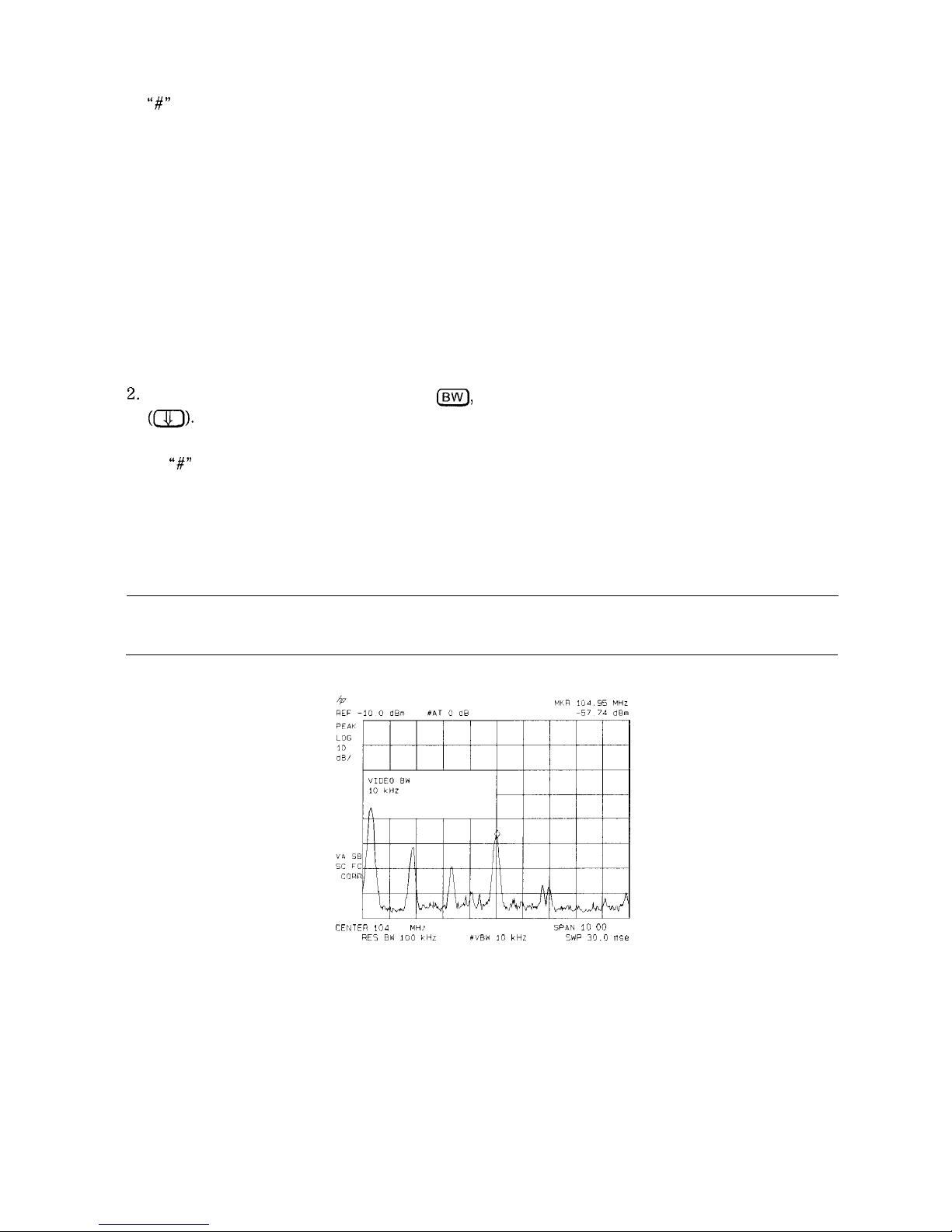
A

“#I’

mark appears next to the RES BW annotation at the lower-left corner of the screen,

indicating that the resolution bandwidth is uncoupled.
As the resolution bandwidth is reduced, the sweep time is increased to maintain calibrated

data.
Example: The video-filter control is useful for noise measurements and observation of

low-level signals close to the noise floor. The video filter is a post-detection low-pass filter that
smoothes the displayed trace. When signal responses near the noise level of the spectrum
analyzer are visually masked by the noise, the video filter can be narrowed to smooth this noise
and improve the visibility of the signal. (Reducing video bandwidths requires slower sweep
times to keep the spectrum analyzer calibrated.)

Using the video bandwidth function, measure the amplitude of a low-level signal.

1. As in the first example, connect an antenna to the spectrum analyzer input. Set the
spectrum analyzer to view a low-level signal.

2.

Narrow the video bandwidth by pressing

Isw],

VID BW AUTO MAN , and the step-down key

((7J-J).

This clarifies the signal by smoothing the noise, which allows better measurement of

the signal amplitude.
A

“#”

mark appears next to the VBW annotation at the bottom of the screen, indicating that

the video bandwidth is not coupled to the resolution bandwidth.
Instrument preset conditions couple the video bandwidth to the resolution bandwidth

so that the video bandwidth is equal to or narrower than the resolution bandwidth. If
the bandwidths are uncoupled when video bandwidth is the active function, pressing

VID BW AUTO MAN (so that AUTO is underlined) recouples the bandwidths. See Figure 3-19.

Note

The video bandwidth must be set wider than the resolution bandwidth when
measuring impulse noise levels.

CEIJTEP 104 93

MH‘~

5P4N

100”MHZ

HE5 BW 100 YHL

#VW I”

lrtiz

SW 30.0 mse

Figure 3-19. Decreasing Video Bandwidth

Making Basic Measurements 3-17

Example: If a signal level is very close to the noise floor, video averaging is another way to
make the signal more visible.

Note

The time required to construct a full trace that is averaged to the desired

degree is approximately the same when using either the video-bandwidth or
the video-averaging technique. The video bandwidth technique completes the
averaging as a slow sweep is taken, whereas the video averaging technique
takes many sweeps to complete the average. Characteristics of the signal
being measured such as drift and duty cycle determine which technique is
appropriate.

Video averaging is a digital process in which each trace point is averaged with the previous

trace-point average. Selecting video averaging changes the detection mode from peak to
sample. The result is a sudden drop in the displayed noise level. The sample mode displays
the instantaneous value of the signal at the end of the time or frequency interval represented
by each display point, rather than the value of the peak during the interval. Sample mode is
not used to measure signal amplitudes accurately because it may not find the true peak of the
signal.

Video averaging clarifies low-level signals in wide bandwidths by averaging the signal and the
noise. As the spectrum analyzer takes sweeps, you can watch video averaging smooth the
trace.

1. Position a low-level signal on the spectrum analyzer screen.

2. Press

(j%ZEJ

More 1 of 3, then VID AVG ON OFF . When ON is underlined, the
video-averaging routine is initiated. As the averaging routine smoothes the trace, low-level
signals become more visible. VID AVG 100 appears in the active function block.

The number represents the number of samples (or sweeps) taken to complete the averaging
routine.

3. To set the number of samples, use the number/units keypad. For example, press
VID AVG ON OFF (so that ON is underlined), 25

IHz).

Turn video averaging off and on again

by pressing VID AVG ON OFF (OFF), VID AVG ON OFF (ON).
The number of samples equals the number of sweeps in the averaging routine.
During averaging, the current sample appears at the left side of the graticule. Changes in

active functions settings, such as the center frequency or reference level, will restart the
sampling. The sampling will also restart if video averaging is turned off and then on again.

Once the set number of sweeps has been completed, the spectrum analyzer continues to
provide a running average based on this set number.

3-l 8

Making Basic Measurements

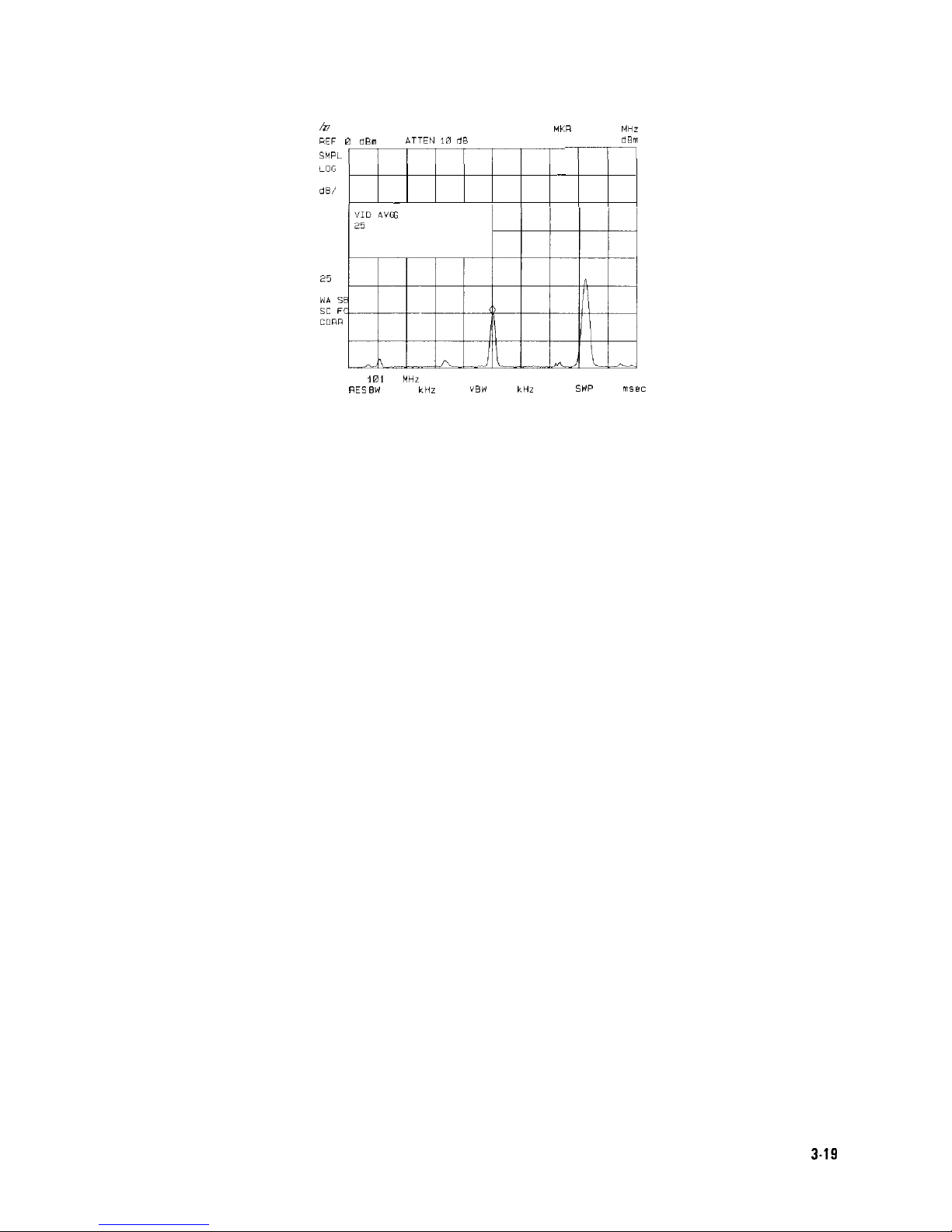
ii?7

MKR 181.73 MHz

REF 0

*Bn

*TEN 10

dR

-60 29

dBm

SMPL

-17

771

LOG

10

-

dB/

-

“ID AVG
25

AVG

25

WA

SB

SC

FC

CURR

t

CENTER

Irnl

73

MHZ

SPAN 10.00 MHZ

RES BW 100 CHz

VBW

30

kHr

SWP

20 rnsec

Figure 3-20. Using the Video Averaging Function

Making Basic Measurements

3.19

Identifying Distortion Products Using the RF Attenuator and
Traces

Distortion from the Analyzer

High-level input signals may cause spectrum analyzer distortion products that could mask the
real distortion measured on the input signal. Using trace B and the RF attenuator, you can
determine which signals, if any, are internally generated distortion products.

Example: Using a signal from a signal generator, determine whether the harmonic distortion
products are generated by the spectrum analyzer.

1. Connect a signal generator to the spectrum analyzer INPUT 500. Set the signal generator
frequency to 200 MHz and the amplitude to 0 dBm.

Set the center frequency of the spectrum analyzer to 400 MHz and the span to 500 MHz:
press

(-1,

400

m,

(SPAN) 500

m.

The signal shown in Figure 3-21 produces

harmonic distortion products in the spectrum analyzer input mixer.

PEAK
LOG

10

dE/

WA SE
SC F(

CDRR

c

L

CENTER

400

0 MHZ

5PAll 500 m

MHZ

RE: SW

3 MHz

YBW 1 MHZ

SWP

20

msec

Figure 3-2

1.

Harmonic

Distortion

2. Change the span to 200 MHz: press (SPAN), 200

INIHz).

3.

Change the attenuation to 0

dB:

press

[AMPLITUDE], ATTEN

AUTO MAN , 0

IdBm_l.

4. To determine whether the harmonic distortion products are generated by the spectrum
analyzer, first save the screen data in trace B.

Press

(ml,

TRACE A B C (until trace B is underlined), then CLEAR WRITE B . Allow the

trace to update (two sweeps) and press VIEW B

, [PEAK SEARCH),

MARKER A . The spectrum

analyzer display shows the stored data in trace B and the measured data in trace A.

5.

Next, increase the RF attenuation by 10

dB:

press

C-1,

ATTEN

AUTO MAN , and the

step-up key

(m)

once. See Figure 3-22.

3-20

Making Basic Measurements

//

1

II / 1

/ 1

CENTER

400

0

MHZ

CENTER

400

0

MHZ

SPAiN 200

SPAiN 200 .o MHZ

.o MHZ

RES BW 1 0 MHZRES BW 1 0 MHZ

“BW 300

kHZ

“BW 300

kHZ

SWP 20

SWP 20 0

nl5P0 nl5P

Figure 3-22.

Figure 3-22. RF

RF

AttenuationAttenuation of 10

of 10

dB

dB

6. Compare the response in trace A to the response in trace B. If the distortion product
decreases as the attenuation increases, distortion products are caused by the spectrum
analyzer input mixer.

Note

When the source signal amplitude is changed between trace A and trace B and
there is a resulting change in the distortion product, this is shown by a change
in the marker amplitude (marker-delta value). An example of the marker-delta
value produced by a change in the distortion product is shown in Figure 3-22.
A change in the distortion product is indicative of high-level input signals
causing circuit overload conditions and producing distortion. This distortion is a
function of the internal hardware of the analyzer. The input signals must be
attenuated to eliminate the interference caused by the internal distortion.

However, if is no change in the distortion product with an increase in
attenuation, the distortion is not caused internally but is a result of distortion
that is present on the input signal as supplied from the signal source. An
example of this is shown in Figure 3-23, where the source signal is not high
enough to cause internal distortion in the spectrum analyzer, therefore, any
distortion that is displayed is present on the input signal.

08hp52:39APR

07.

1943

MKR

a 0

HZ

HEF

-100dBm

iiAT

10 dR

.c7

dB

PEAK

LOG

10

c1 B /

CENTER

a00

0

MHZ SPA!4 200

0

MHZ

RES

BW

1.0

MHZ VBW

300

kHL

SW 20

0 nl5e

Figure 3-23. No Harmonic Distortion

Making Basic Measurements

3-21

Third-Order Intermodulation Distortion

Two-tone, third-order intermodulation distortion is a common problem in communication
systems. When two signals are present in a system, they can mix with the second harmonics
generated and create third-order intermodulation distortion products, which are located close
to the original signals. These distortion products are generated by system components such as
amplifiers and mixers.

Example: Test a device for third-order intermodulation. This example uses two sources, one
set to 300 MHz and the other to approximately 301 MHz. (Other source frequencies may be
substituted, but try to maintain a frequency separation of approximately 1 MHz.)

1. Connect the equipment as shown in Figure 3-24.

Figure 3-24. Third-Order Intermodulation Equipment Setup

2. Set one source to 300 MHz and the other source to 301 MHz for a frequency separation of
1 MHz. Set the sources equal in amplitude (in this example, the sources are set to -5

dBm)

3. Tune both signals onto the screen by setting the center frequency between 300 and

301 MHz. Then, using the knob, center the two signals on the display. Reduce the frequency
span to 5 MHz for a span wide enough to include the distortion products on the screen. To

be sure the distortion products are resolved, reduce the resolution bandwidth until the

distortion products are visible. Press

(BW),

RES BW , and then use the step-down key

((J-J)

to

reduce the resolution bandwidth until the distortion products are visible.

4. For best dynamic range, set the mixer input level to -40

dBm

and move the signal to the

reference level: press

C-1,

More 1 of 3 , MAX MXR LEVEL , 40

m.

The spectrum analyzer automatically sets the attenuation so that a signal at the reference
level will be a maximum of -40 dBm at the input mixer.

5. To measure a distortion product, press

[PEAK SEARCH)

to place a marker on a source signal.

To activate the second marker, press MARKER A . Using the knob, adjust the second marker
to the peak of the distortion product that is beside the test tone. The difference between
the markers is displayed in the active function block.

3-22 Making Basic Measurements

To measure the other distortion product, press

SPEAK SEARCH],

NEXT PEAK . This places a

marker on the next highest peak, which, in this case, is the other source signal. To measure
the difference between this test tone and the second distortion product, press MARKER A
and use the knob to adjust the second marker to the peak of the second distortion product.

See Figure 3-25.

J@

MKR a I 025

MHz

REF 0

dBm

ATTEN 40 dB

-54.04 dB
PEAK
LOG

10

dB/

WA SE
SC

FS

CORR

t-

L

CENTER 300.650 MHz

SPAN 5

000 MHZ

XRFS RW

7

kH7

“RW-4kH7

SWP1 7

SPr

Figure 3-25. Measuring the Distortion Product

Making Basic Measurements 3-23

Using the Analyzer As a Receiver in Zero Frequency Span

The spectrum analyzer operates as a fixed-tuned receiver in zero span. The zero span mode can
be used to recover modulation on a carrier signal.

Center frequency in the swept-tuned mode becomes the tuned frequency in zero span. The
horizontal axis of the screen becomes calibrated in time, rather than frequency. Markers

display amplitude and time values.
The following functions establish a clear display of the video waveform:

w

Trigger stabilizes the waveform trace on the display by triggering on the modulation

envelope. If the signal’s modulation is stable, video trigger synchronizes the sweep with the
demodulated waveform.

n Linear mode should be used in amplitude modulation (AM) measurements to avoid distortion

caused by the logarithmic amplifier when demodulating signals.

n Sweep time adjusts the full sweep time from 20 ms (20 ps in zero span with Option 101) to

100 s. The sweep time readout refers to the full lo-division graticule. Divide this value by 10

to determine sweep time per division.

w

Resolution and video bandwidth are selected according to the signal bandwidth.

Each of the coupled function values remains at its current value when zero span is activated.
Video bandwidth is coupled to resolution bandwidth. Sweep time is not coupled to any other
function.

Note

Capability for measuring AM or FM demodulation is available if Option 102,

103, or 301 is installed in your spectrum analyzer. Refer to “Demodulating and

Listening to an AM or FM Signal” in Chapter 4 for more information.

Example: View the modulation waveform of an AM signal in the time domain.

1. To obtain an AM signal, you can either connect an antenna to the spectrum analyzer input
and tune to a commercial AM broadcast station or you can connect a source to the spectrum

analyzer input and set the percent modulation of the source. (If a headset is used with the

VIDEO OUT connector, the spectrum analyzer will operate as a radio.)

2. First, center and zoom in on the signal in the frequency domain (see “Decreasing the
Frequency Span Using the Marker Track Function”). Be sure to turn off the marker track
function, since the marker track function must be off for zero span. See Figure 3-26.

3.24

Making Basic Measurements

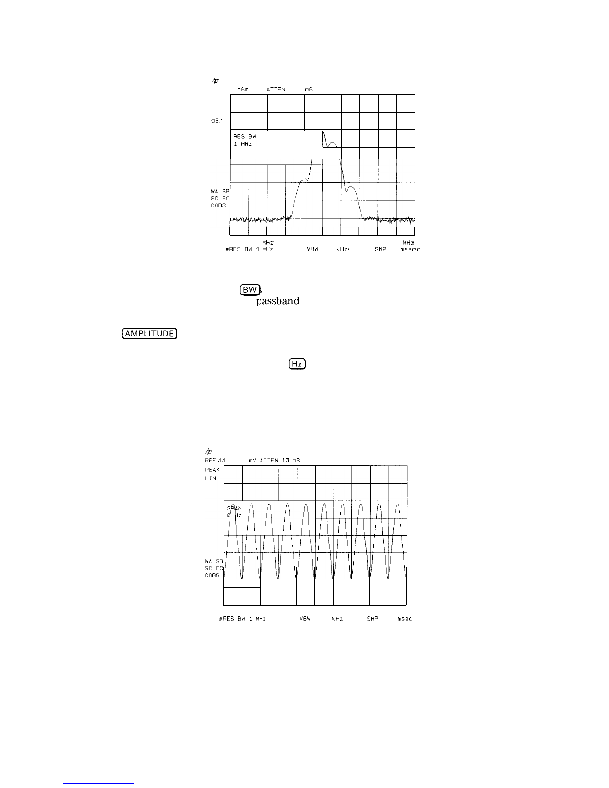
44

REF
PEAK
LOG

10

dB/

0

dBm

ATTEN

10

dB

I I

CENTER 300 00

CENTER 300 00 MHz

MHz SPAN 20.00SPAN 20.00 MHzMHz

#RES BW 1

#RES BW 1 MHZ

MHZ VBWVBW

300

kHz

300

kHz

SW

20

msec

SW

20

msec

Figure 3-26. Viewing an AM SignalFigure 3-26. Viewing an AM Signal

3. To demodulate the AM, press

[Bw).

Increase the resolution bandwidth to include both

sidebands of the signal within the

passband

of the spectrum analyzer.

4. Next, position the signal peak near the reference level and select a linear voltage display.
Press

[AMPLITUDE]

and change the reference level, then press SCALE LOG LIN to underline

LIN.

5. To select zero span, either press (SPAN), 0

IHz)

or press ZERO SPAN . See Figure 3-27. If
the modulation is a steady tone (for example, from a signal generator), use video trigger
to trigger on the waveform and stabilize the display. Adjust the sweep time to change the
horizontal scale.

Use markers and delta markers to measure time parameters of the waveform.

4

REF dd 61 mVATTEN 10

dB

CENTER 300 000 MHZ SPAN 0 HZ

XRES BW i

MHz VBW

300

kHz

SWP

20

msec

Figure 3-27. Measuring Modulation in Zero Span

Making Basic Measurements 3-25

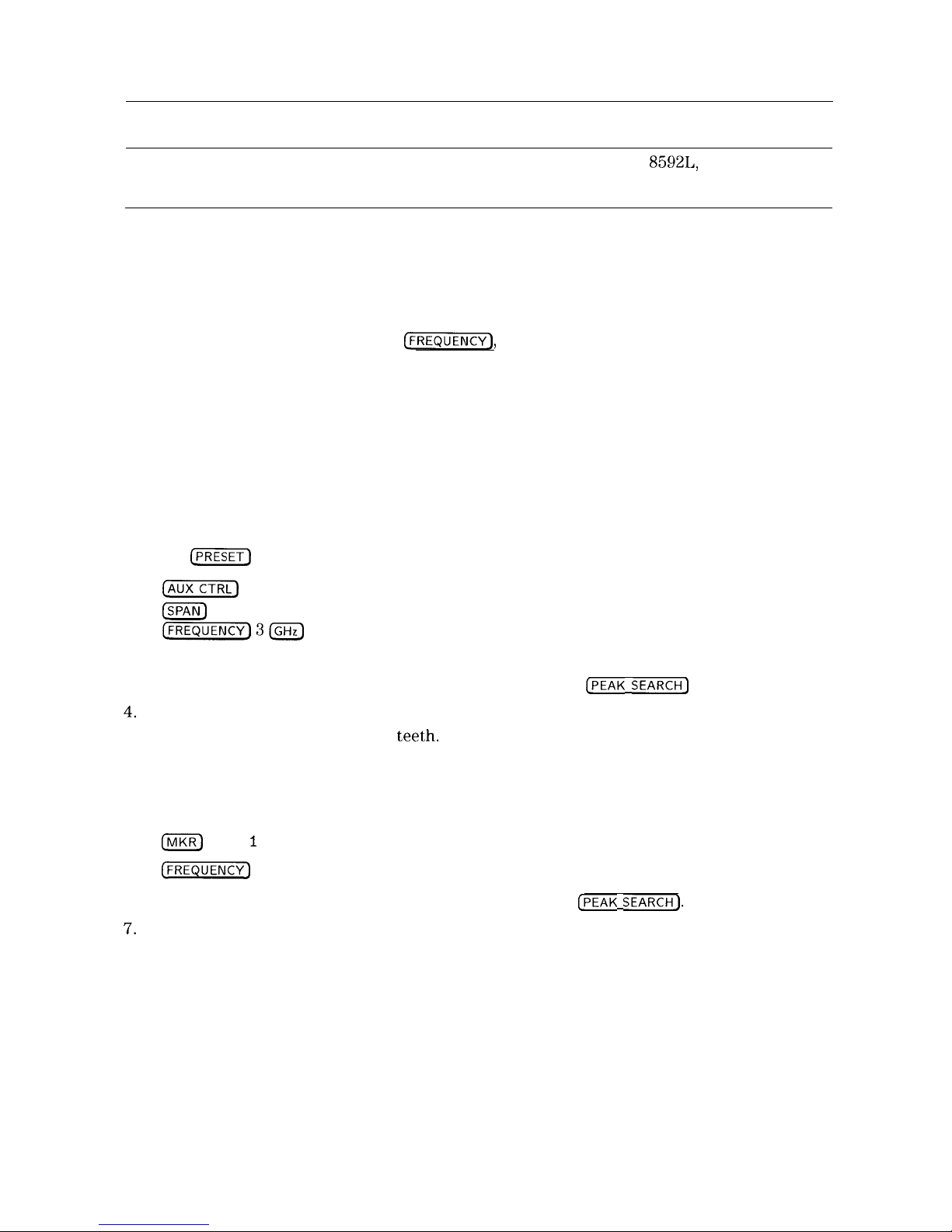
Measuring Signals Near Band Boundaries Using Harmonic Lock

Note

This application should only be performed using an HP

8592L,

HP 85933,

HP 85953, or HP 85963.

When measuring signals at or near a band crossing, use the lowest band having a specified
upper frequency limit that will include the signal of interest. See specifications and

characteristics in your calibration guide for your instrument for harmonic band specifications.

Using harmonic lock, and choosing the lowest possible band to analyze a signal, ensures the

best specified measurement accuracy.
To lock onto a specific harmonic, press

C-1,

Band Lock , BND LOCK ON OFF (so that
ON is underlined), or select a band (see specifications and characteristics in your calibration
guide for your instrument for band specifications). After setting the harmonic lock, only center
frequencies and spans within the frequency range of the harmonic band may be entered. The
span is automatically reduced to accommodate a center frequency specified near the end of the

band ‘range.

Example:

1. Connect 100 MHz COMB OUT to the spectrum analyzer input. The HP 85953 does not have
a 100 MHz COMB OUT signal, so it cannot be used for this measurement example. (An
external source must be substituted.)

2. Press

[PRESET]

and then the following keys:

(mCTRL_)

COMB GEN ON OFF (ON)

ISPAN)

350 (MHz)

[FREQUENCY)3m

Band Lock BND LOCK ON OFF (ON)

3. Place a marker on the farthest peak to the left by using the

[PEAK SEARCH]

key.

4.

Press MARKER A , NEXT PK RIGHT, NEXT PK RIGHT to show the frequency and amplitude

difference between the two comb teet,h.
You will see three comb teeth on your display. The spectrum analyzer is locked in band 1

and will not allow multiband sweeps. See Figure 3-28.

5. To see a multiband sweep, press the following keys:

(MKR)

More 1 of 2 MARKER ALL OFF

(FREQUENCY]

Band Lock BND LOCK ON OFF (OFF)

6. Place a marker on the farthest peak to the left by pressing

[PEAK SEARCH].

‘7.

Press MARKER A . Use NEXT PK RIGHT to place a marker on the farthest peak to the right.

The marker readout displays the frequency and amplitude difference between the two comb
teeth. See Figure 3-29.

3-26 Making Basic Measurements

4Q

MKR a

200.4 MHz

REF 0

dBm

ATTEN

10 dB

-2

02 dB

LOG

10

I I II i

dE/

MARKER

C

,

CENTER 12.9000 GHr SPAN 350.0 MHz

RES BW 3 MHz “BW1MHZ SWP

20

msec

Figure 3-28. Using Harmonic Lock

Note

The comb frequencies have a 100 MHz spacing.

b

REF
PEAK
LOG

10

dE/

MKR A

201.3 MHz

dBm

ATTEN

10 dB

MARKER

C

CENTER 12.9000 GHr

RES

B’*I

3 MHz

SPAN 350.0 MHz

SW

40

msec

Figure 3-29. Harmonic Locking Off

Making Basic Measurements

3.27

Making Measurements

What You’ll Learn in This Chapter

This chapter demonstrates spectrum analyzer measurement techniques with examples
of typical applications; each application focuses on different features. The measurement
procedures covered in this chapter are listed below.

n Measuring amplitude modulation using the fast Fourier transform function.

w

Stimulus-response measurements using the built-in tracking generator (Option 010 or 011).

n Demodulating and listening to an AM or FM signal (Option 102 or 103 only).

w

Triggering on a selected line of a video picture field (Options 101 and 102, or Option 301

only).

n Making a reflection calibration and measurements.

w

Using the Gate Utility to simplify time-gated measurements (Option 105 only).

w

Using the time-gated spectrum analyzer capability (Option 105 only).

n Using the one-button measurements to measure N

dB

bandwidth, percent amplitude

modulation, and third order intercept

(TOI).

w

Using the power measurement functions to make transmitter measurements.

To find descriptions of specific spectrum analyzer functions refer to Chapter 7 “Key

Descriptions”.

‘Making Measurements 4-1

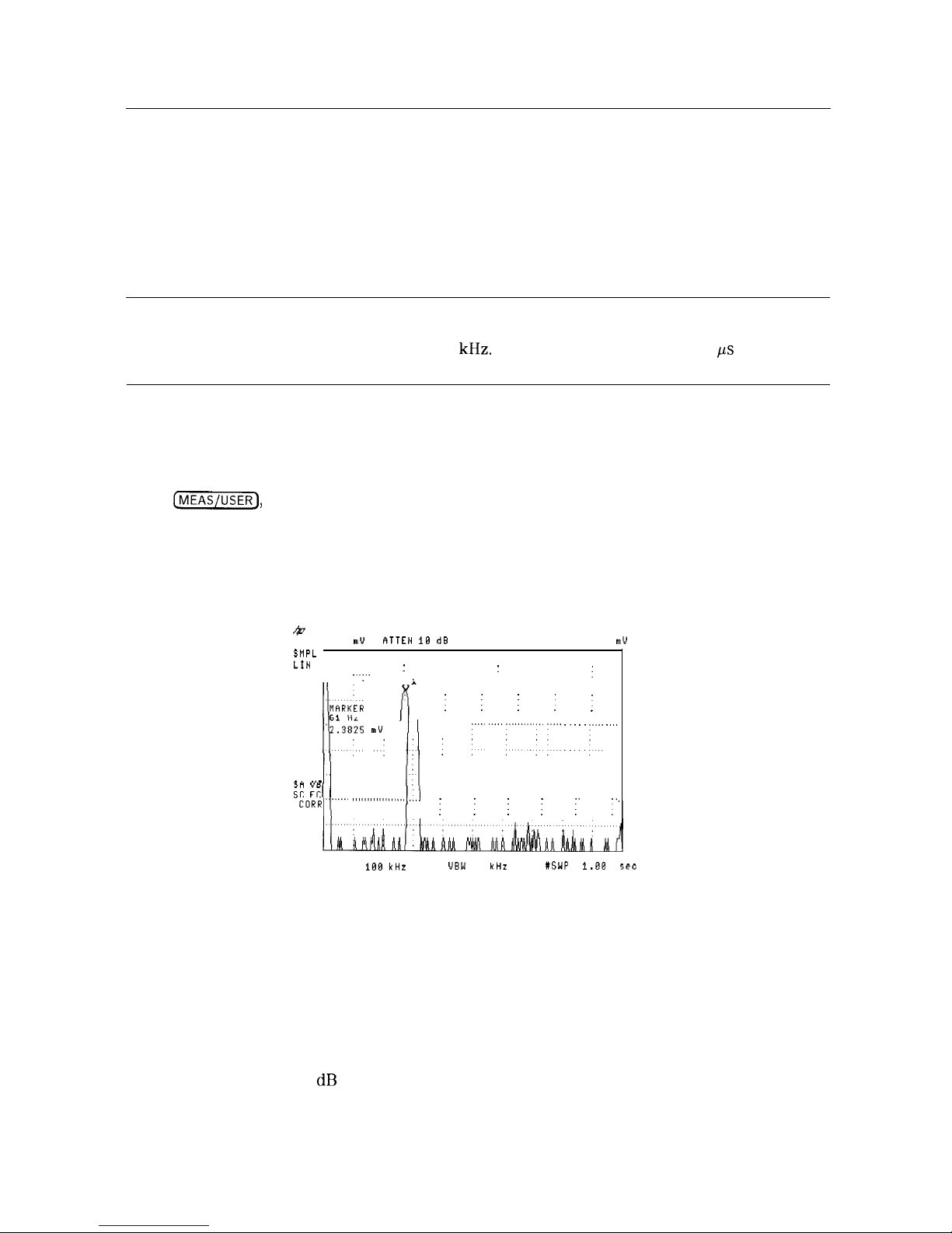
Measuring Amplitude Modulation with the Fast Fourier
Transform Function

A Fourier transform, transforms time domain data (zero span) into the frequency domain.
The fast Fourier transform (FFT) function of the spectrum analyzer allows measurements
of amplitude modulation (AM). It is commonly used to measure AM at rates that cannot be
measured in the normal frequency domain due to spectrum analyzer limitations on narrow
resolution bandwidths. For a given AM rate, the FFT function can generate a trace faster than
using the frequency domain for the equivalent spectrum analyzer measurement.

Note

The fast ADC Option 101 extends FFT operation. The standard spectrum

analyzer has sweep times (in zero span) up to 20 ms and allows FFT stop
frequencies from 20 Hz to 10

kHz.

With Option 101, spans of 20 ps can be used

and FFT stop frequencies up to 10 MHz are available.

The FFT function calculates the magnitude of each frequency component from a block of
time-domain samples of the input signal. It uses a flat top filter response. This implementation
is a post-detection Fourier transform and it cannot be used to resolve continuous wave or
carrier signals.

When

IjjJ

FFT Menu , and SINGLE FFT are pressed, sample-detection mode is selected
and a sweep is taken to obtain a sample of the input signal. Then the spectrum analyzer
executes a series of computations on the time data to produce the frequency-domain results.

CONTINUS FFT can be used instead of SINGLE FFT and the spectrum analyzer will be put in

continuous sweep mode with an FFT being performed at the end of each sweep.

/;o

WKR 61 HZ

REF 15.83 muhTTEN 1B dB

2.3825

mV

SWPL

'.IN

: :

I

.;

i

llFyR(bR

/j : : : :

:

/y3y

n”:

,:\

:

I ,I.., i,,.~ ~ . . . . . . ..,,

** ‘I-

II

ii: 3 I

II

""""1'1"""

,,,,,,,,,,,,,,,,.,

I...1

, :

: : : :.

:.

FFT START 0 Hz

FFT STOP

200 Hz

RES BW 188 kHz

UBW 38 kHz

XSWP 1.88 set RT

Figure 4-l. FFT Annotation

Some of the screen annotation is altered when the FFT function is active. The left edge of
the graticule is relabeled FFT START and represents 0 Hz relative to the carrier. The right
edge of the graticule is relabeled FFT STOP and is the maximum FFT frequency used in the
transformation. The annotation LIN in the upper left corner refers to the scale of the incoming
data being transformed. The FFT results, which are being displayed, are always in LOG scale.

The carrier appears at the left edge of the graticule with the modulation sidebands and any
distortion appearing along the horizontal axis. The amplitude relationships of all the signals

are the same as they would be if the components were displayed with normal swept-tuned

operation in log mode, 10 dB per division.

4-2 Making Measurements

If the FFT stop frequency is less than the highest harmonic of the AM modulation, than the
FFT results may include

aliased

signals. That is, it will include some signals that are being
displayed at the wrong frequency. The sweep time affects the sample rate and must be
optimized to avoid aliasing.

The single and continuous FFT functions require a specific spectrum analyzer setup before they

can be activated. First, an AM signal is demodulated in the time domain. In order to do this,
the resolution bandwidth is widened to include the signal sidebands within the

passband

of
the spectrum analyzer. Next, zero span is selected so that the spectrum analyzer operates as a
fixed-tuned receiver. Tuning is centered around the AM carrier.

The MARKER+ AUTO FFT

softkey

activates the FFT function with very little preliminary setup

required. Two examples of using the FFT function are included in this section.

n First example: uses the manual FFT functions.
n Second example: uses the automatic FFT measurement.

Note

After the FFT function is used, the markers are still in FFT mode for use in
evaluating data. Turn off the FFT markers before attempting to use markers in

the normal fashion. Press FFT OFF in the FFT menu to turn off the markers
and exit the FFT measurement.

Example 1: Use the manual FFT measurement to look at 60 Hz AM modulation.

1. Connect a signal generator to the spectrum analyzer INPUT 500. Adjust the signal
generator to produce an AM signal with a 60 Hz modulation frequency.

2. Press [FREQUENCY_) and set the spectrum analyzer center frequency to the frequency of the
modulated input signal. Press

m),

10 MHz. Press

[FREQUENCY)

again and center the

signal on the spectrum analyzer display.

3. Press

LSPAN),

1 MHz. Press

[FREQUENCY)

and center the signal on the spectrum analyzer

display again.

4. Press

m,

100 kHz. (Re-center the signal, if necessary.)

Press

m

200 kHz, re-centering the signal again if it is necessary.

5.

Press VID BW

AUl’fl

MAN , 1 kHz. The video bandwidth should be about ten times greater

than the highest modulation frequency of interest for the best amplitude accuracy.

6. Press REF LVL and turn the knob to change the reference level, placing the signal peak
within the top division of the screen. The signal peak must be below the reference level.

The signal amplitude moves up and down because the spectrum analyzer catches the signal
at different points of modulated amplitude each time it sweeps.

‘7.

Change the amplitude scale to linear by pressing

IjAMPL’TUDE]

and SCALE LOG LIN so that
LIN is underlined. The FFT will give incorrect results when the spectrum analyzer is in Log
mode.

Press REF

LVL

and place the signal peak within the top division of the screen.

8. Press

m,

0 Hz. The spectrum analyzer now operates as a fixed-tuned receiver.

9.

Press

(MEAS~JSER],

FFT Menu, and CONTINUS FFT . The spectrum analyzer will now be

taking

FFTs

continuously, updating the measurement at the end of every sweep.

Press FFT STOP FREQ , 250 Hz. This sets the spectrum analyzer to include the fourth
harmonic of the 60 Hz modulation signal on the screen.

Making Measurements 4-3

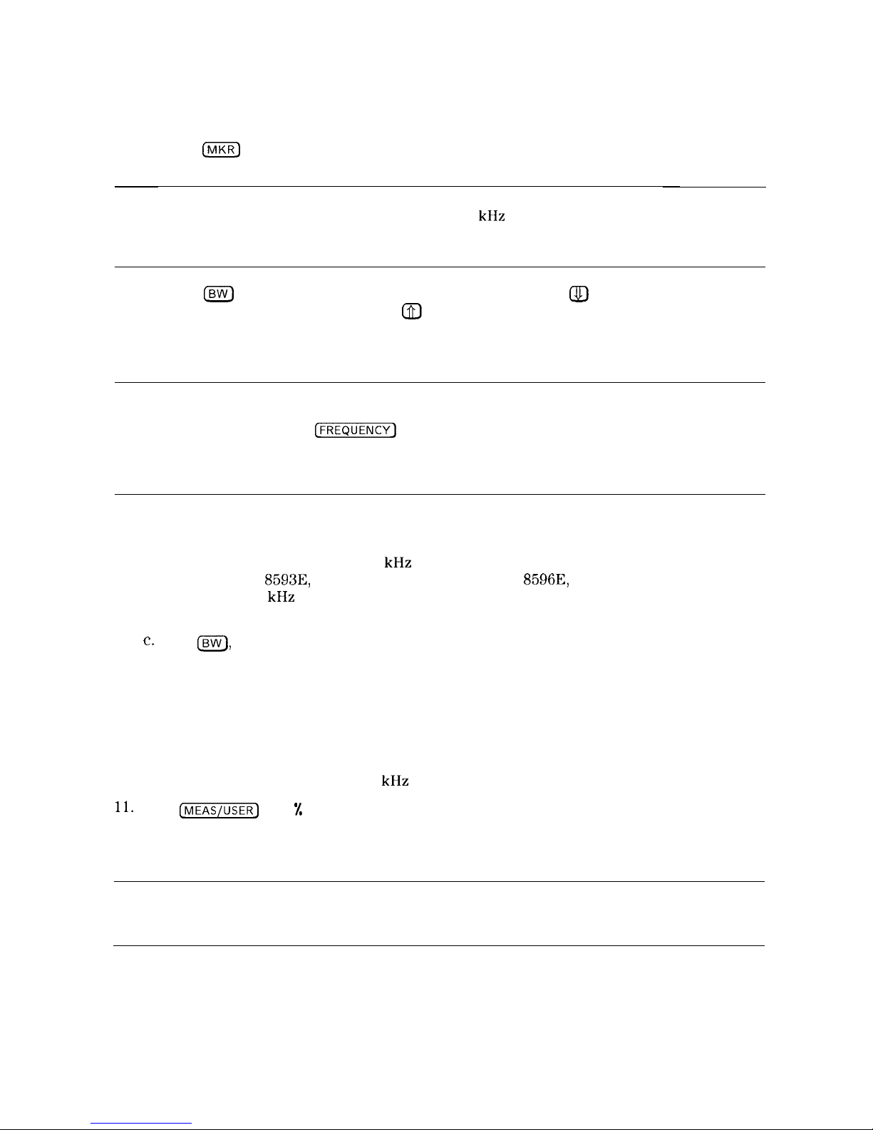
10. To confirm that the resolution bandwidth and video bandwidth are correct for measuring
the modulation amplitude, use the following procedure:

a. Press

(MKRI

and use the knob to move the marker to the desired modulation signal. In

this example, place the marker on the 60 Hz fundamental modulation signal.

Note

For HP 8590L with Option 713 or HP 8592L with Option 713 the resolution
bandwidth must be left at about 100 kHz to accommodate frequency drift of
the spectrum analyzer. If you are using an HP 8590L with Option 713, or an
HP 8592L with Option 713, do not do step b.

b. Press

CBW)

and decrease the resolution bandwidth using the @J key, until measured

signal amplitude drops. Then press a to increase the bandwidth until the signal

amplitude stops increasing and stays the same, or until the maximum resolution

bandwidth is reached. Use the narrowest bandwidth that does not cause a change in the

signal amplitude.

Note

As the resolution bandwidth is stepped down, the modulated signal must be
re-centered in the filter bandwidth. This is a zero span display. To center the
signal, select

[FREQUENCY)

and adjust the center frequency to maximize the

amplitude of the trace. If this is not done, the signal amplitude can decrease
due to off tuning of the spectrum analyzer and not because of the resolution

bandwidth chosen.

For the best amplitude accuracy, the resolution bandwidth should be about 10 times
greater than the highest modulation frequency of interest.

For the 60 Hz fundamental, a 1 kHz resolution bandwidth works well. (For the
HP 85913, HP

8593E,

HP 85943, HP 85953, and HP

8596E,

if harmonics are not a
concern, a 100 kHz resolution bandwidth can be used and it will provide a faster update
rate.)

C.

Press

IBW),

VID BW AUTO MAN (MAN) and use the step keys to decrease the video

bandwidth until the amplitude of the measured signal drops. Then step the bandwidth
up until the signal amplitude stops increasing, or until the maximum video bandwidth is
reached. Use the narrowest video bandwidth that does not cause a change in the signal
amplitude.

For the best amplitude accuracy, the video bandwidth should be about 10 times greater
than the highest modulation frequency of interest.

For the 60 Hz fundamental, a 1 kHz video bandwidth works well.

11.

Press

[MEAS/USERJ

and % AM ON OFF so that ON is underlined. The spectrum analyzer
reads out the percent AM of the largest modulation frequency. An arrow indicates the
signal being measured (see Figure 4-l). This measurement does not include all of the
harmonics of the modulating signal.

Note

The percent AM function will not run if the SIGNAL CLIPPED error message
is being displayed. Increase the reference level until the error message goes
away.

4-4 Making Measurements

Note

When the FFT measurement is active, pressing the

CMEAS/USER)

key will cycle

between the MEASUSER and FFT menus.

4.7

MKR

1.817

LHZ

REF .B

dBrn

RTTEH i@

dB

-45.25

dBrn

No

u5er

SMPL

Men”

LOG
2,

:

.:

I

I

FFT

START B HZ

FFT

STOP 6.667

k”Z

RES BW 18

k”Z

“BW 9.8

k”Z

SWP

38.8 m5e.2

R

Figure 4-2. Percent Amplitude Modulation Measurement

Example 2: Use the automatic FFT measurement to look at 60 Hz AM modulation.

1. Connect a signal generator to the spectrum analyzer INPUT

509.

Adjust the signal generator

to produce an AM signal with a 60 Hz modulation frequency.

2. Press

[FREQUENCY)

and set the spectrum analyzer center frequency to the frequency of the

modulated input signal. Press

m),

10

m.

Press

[FREQUENCY)

to keep the signal on the

spectrum analyzer display.

3.

Press

[MEAS~USER),

FFT Menu, and MARKER

+

AUTO FFT . This initiates the FFT function and

activates a marker.

4. Use the knob to place the marker on the AM modulated signal and press
MARKER--+ AUTO FFT again. The spectrum analyzer will perform the following steps:

a. Save the present instrument state in state register 8.

b. Reduce the span to zoom in on the signal.

c. Set the detector mode to sample.
d. Set the scale to linear.

e. Change the span

to zero

span.

f. Start the continuous FFT function.

g. Set the FFT stop frequency to 10 kHz.

5. Press FFT STOP

FREQ

, 250

a).

This sets the spectrum analyzer to include the fourth

harmonic of the 60 Hz modulation signal on the screen.

6. To confirm that the resolution bandwidth and video bandwidth are correct for measuring the

modulation amplitude, use the following procedure:
a. Press

m

and use the knob to move the marker to the desired modulation signal. In

this example, place the marker on the 60 Hz fundamental modulation signal.

Note

For HP 8590L with Option 713 or HP 8592L with Option 713 the resolution
bandwidth must be left at about 100 kHz to accommodate frequency drift of
the spectrum analyzer. If you are using an HP 8590L with Option 713, or an
HP 8592L with Option 713, do not do step b.

Making Measurements 4-5

b. Press

(Bw)

and decrease the resolution bandwidth using the Q) key, until measured signal

amplitude drops. Then press @) to increase the bandwidth until the signal amplitude

stops increasing and stays the same, or until the maximum resolution bandwidth is

reached. Use the narrowest bandwidth that does not cause a change in the signal
amplitude.

Note

As the resolution bandwidth is stepped down, the modulated signal must be
re-centered on the spectrum analyzer display. If this is not done, the signal
amplitude can decrease due to off tuning of the spectrum analyzer and not

because of the resolution bandwidth chosen.

For the best amplitude accuracy, the resolution bandwidth should be about 10 times
greater than the highest modulation frequency of interest.

For the 60 Hz fundamental, a 1 kHz resolution bandwidth works well. (For the HP

8591E,

HP 85933, HP 85943, HP 85953, and HP 85963, if harmonics are not a concern, a

100 kHz resolution bandwidth can be used and it will provide a faster update rate.)

c.

Press

Isw),

VID BW AUTO MAN (MAN) and use the step keys to decrease the video
bandwidth until the amplitude of the measured signal drops. Then step the bandwidth
up until the signal amplitude stops increasing, or until the maximum video bandwidth is
reached. Use the narrowest video bandwidth that does not cause a change in the signal
amplitude.

For the best amplitude accuracy, the video bandwidth should be about 10 times greater
than the highest modulation frequency of interest.

For the 60 Hz fundamental, a 1 kHz video bandwidth works well.

‘7.

Press

[jJ

and % AM ON OFF so that ON is underlined. The spectrum analyzer reads
out the percent AM of the largest modulation frequency. An arrow indicates the signal being
measured (see Figure 4-l). This measurement does not include all of the harmonics of the

modulating signal.

Note

The percent AM function will not run if the SIGNAL CLIPPED error message
is being displayed. Increase the reference level until the error message goes
away.

Note

Note

To return to the spectrum analyzer state prior to running the FFT function,
press the FFT OFF softkey. This turns off the FFT function. Press

[RECALL],

INTERNAL

+STATE

, and 8 to recall the state from state register 8.

When the FFT measurement is active, pressing the

[MEAS~USER]

key will cycle

between the MEASUSER and FFT menus.

4-6 Making Measurements

Stimulus-Response Measurements

Note

This application should only be performed using an HP 8590L or HP 85913 with
Option 010 or 011, or using an HP 85933, HP 85943, HP 85953, or HP 85963
with Option 010.

What Are Stimulus-Response Measurements?

Stimulus-response measurements require a source to stimulate a device under test (DUT), a
receiver to analyze the frequency-response characteristics of the DUT, and, for return-loss
measurements, a directional coupler. Characterization of a DUT can be made in terms of its
transmission or reflection parameters. Examples of transmission measurements include flatness

and rejection. A reflection measurement is return loss.
A spectrum analyzer combined with a tracking generator forms a stimulus-response

measurement system. With the tracking generator as the swept source and the spectrum

analyzer as the receiver, operation is analogous to a single-channel scalar network analyzer.
A narrow-band system has a wide dynamic measurement range, but the tracking generator’s
output frequency must be made to precisely track the spectrum analyzer input frequency. This
wide dynamic range will be illustrated in the following example. Figure 4-3 shows the block
diagram of a spectrum analyzer and tracking-generator system.

SPECTRUM

AI‘JAL YZER

I

:‘---) ~-~~~2~~

I

T

\’

2-+-gg

Ii AMP

-i

I

TRACK I

r\iG

GEI\IERATOR

v

L..

____

4

------

Fi\,;;~9-fgF.

;F

Figure 4-3.

Block Diagram of a Spectrum Analyzer/Tracking-Generator Measurement System

Note

The HP 85630A Transmission/Reflection Test Set with the HP 85714A Scalar
Measurement Personality is recommended for making transmission and
reflection measurements with your spectrum analyzer. The scalar measurement
personality provides simple menu-driven functions to make fast, accurate
scalar network analysis measurements with your spectrum analyzer and test
set.

Making Measurements 4-7

Using a Spectrum Analyzer with a Tracking Generator

The procedure below describes how to use the built-in tracking generator system of the

HP 85913 Option 010 spectrum analyzer to measure the rejection of a low-pass filter which

is a type of transmission measurement. Illustrated in this example are the functions in the

tracking-generator menu, such as adjusting the tracking-generator output power, source
calibration, and normalization. Conducting a reflection measurement is similar and is covered
in “Making Reflection Calibration Measurements”.
or Application Note

150-7,

for more information.

Refer to the HP Spectrum Analyzer Seminar,

Stepping through the Measurement

There are four basic steps in performing a stimulus-response measurement, whether it be

a transmission or reflection measurement: set up the spectrum analyzer settings, calibrate,

normalize, and measure.

1. If necessary, perform the self-calibration routine for the tracking generator described in
“Performing the Tracking Generator Self-Calibration Routine” in Chapter 2.

2. To measure the rejection of a low-pass filter, connect the equipment as shown in Figure 4-4.
This example uses a filter with a cut-off frequency of 300 MHz as the DUT.

SPECTRUM ANALYZER

RF

OlJi

INPUT

SOS7

Figure 4-4. Transmission Measurement Test Setup

3. Activate the tracking generator menu by pressing

(%ZiK]

and Track Gen . To activate

the tracking-generator power level, press SRC PWR ON OFF until ON is underlined
(see Figure 4-5).

Caution

Excessive signal input may damage the DUT. Do not exceed the maximum

power that the device under test can tolerate.

Note

To reduce ripples caused by source return loss, use 10 dB or greater tracking
generator output attenuation. Tracking generator output attenuation is
normally a function of the source power selected. However, the output

attenuation may be controlled by using SRC ATN AUTO MAN . (There is no

output attenuation in the HP

85901,

with Option 010 or Option 011.) Refer to

specifications and characteristics in your calibration guide for more information

on the relationship between source power and source attenuation.

4-8 Making Measurements

&&

REFREF

dBm

ATTEN

10

d8

PEAKPEAK
LOGLOG

10

dB/dB/

/

WA SBWA

SB

SC FCSC FC

CORRCORR

1

CENTER 900 MHZ

CENTER

900

MHZ

SPAN

1

SPAN 1

800 GHr

800

GHr

RES BW 3

MHZ

RES BW 3

MHZ “BW“BW 1 MHZ1MHZ SWPSWP

20

msec20msec

Figure 4-5. Tracking-Generator Output Power Activated

4. Put the sweep time of the analyzer into stimulus-response auto-coupled mode by pressing
More 1 of 2 , then SWP CPLG SR SA until SR (stimulus-response mode) is underlined.

Auto-coupled sweep times are usually much faster for swept-response measurements than
they are for spectrum analyzer measurements.

Note

In the stimulus-response mode, the Q (reactance versus resistance) of the
DUT can determine the fastest rate at which the spectrum analyzer can be
swept. To determine whether the analyzer is sweeping too fast, slow the
sweep time and note whether there is a frequency or amplitude shift of the
trace. Continue to slow the sweep time until there is no longer a frequency or
amplitude shift.

5. Since we are only interested in the rejection of the low-pass filter, tune the spectrum
analyzer center frequency so that the roll-off of the filter comprises the majority of the trace
on the display (see Figure 4-6).

ik
FIEF

0

dBm

ATTEN

10

dB

PEAKPEAK
LOGLOG

1818

dB/dB/

CENTER 443 6 MHZ SPAN 5061.0 MHz

FE5 BW

3

MHZ

vow1MHZ

SWP 20

msec

Figure 4-6. Spectrum Analyzer Settings According to the Measurement Requirement

Making Measurements 4-9

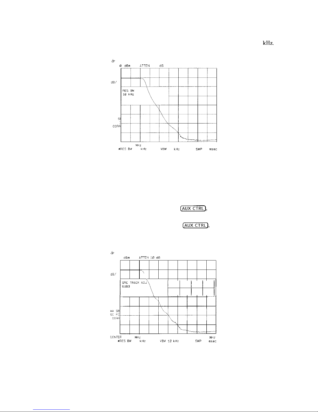
6. Decrease the resolution bandwidth to increase sensitivity, and narrow the video bandwidth
to smooth the noise. In Figure 4-7, the resolution bandwidth has been decreased to 10

kHz.

40

REF 0

dBm

ATTEN

10 dB
PEAK
LOG

10

dB/

VP

St

SC F!

CO!a

CENTER 443 6

MHZ

SPAN 500.0

MHz

#RES EW

10

kHz

“BW

10 kHZ

SWP

50

msec

Figure 4-7. Decrease the Resolution Bandwidth to Improve Sensitivity

Adjusting the resolution bandwidth may result in a decrease in amplitude of the signal.
This is known as a tracking error. Tracking errors occur when the tracking generator’s
output frequency is not exactly matched to the input frequency of the spectrum analyzer.
Tracking errors are most notable when using narrow resolution bandwidths. Tracking
error can be compensated manually or automatically. In narrow bandwidths, the manual
method of adjusting the tracking is usually faster than the automatic tracking adjustment.

To compensate for the tracking error manually, press

(AUX],

Track Gen , and

MAN TRK ADJUST , then use the knob to adjust the trace for the highest amplitude. To

compensate for the tracking error automatically, press

(-1,

Track Gen , then

TRACKING PEAK.

h

REF 0

dBm

ATTEN I0 dB

PEAK
LOG

10

dB/

:

\

/ ;W;RACK ADJ\

~

( 1 j

~

CENlEn

443 6

MHz

SPAN 500.0

MH7

XRES

EW

10

CllZ

“BW

10 kHZ

SWP

50

msec

Figure 4-8. Manual Tracking Adjustment Compensates for Tracking Error

4-10 Making Measurements

Note

If the automatic tracking routine is activated in a narrow resolution bandwidth,
it usually is not necessary to use the tracking adjust again when increasing the
resolution bandwidth.

7. To make a transmission measurement accurately, the frequency response of the test system
must be known. To measure the frequency response of the test system, connect the cable

(but not the DUT) from the tracking generator output to the spectrum analyzer input. Press

Cm],

TRACE A B C (so B is underlined), CLEAR WRITE B , BLANK B . The frequency

response of the test system is now stored in trace B.

8.

To normalize, reconnect the DUT to the spectrum analyzer. Press

(TRACE],

More 1 of 3 ,

NORMLIZE ON OFF until ON is underlined. Press NORMLIZE POSITION to activate the
display line. This display line marks the normalized reference position, or the position
where 0 dB insertion loss (transmission measurements) or 0 dB return loss (reflection
measurements) will normally reside. Using the knob results in a change in the position of
the normalized trace, within the range of the graticule.

Normalization eliminates the frequency response error of the test system. When
normalization is on, trace math is being performed on the active trace. The trace math
performed is trace A minus trace B plus the display line, with the result placed into trace
A. Remember that trace A contained the measurement trace, trace B contained the stored
calibration trace, and DL (display line) represents the normalized reference position. Note
that the units of the reference level,

dB,

reflect this relative measurement.

b
REF

e

PEAK
LOG

10

dB/

DL

-6

6

dB

1 dBm

ATTEN

10 dB

I

I I I I I II I

I

i

DISPLAY LINE

-6

6 dB

CENTER 443 6 MHz SPAN

500.0

MHz

#RES BW

10

kHz

VQW10kHz

SWP

50

nlsec

Figure 4-9. Normalized Trace

9. To measure the rejection of the filter at a given frequency, press

Ir\nKRl,

and enter the
frequency. For example, enter 350 MHz. The marker readout displays the rejection of the
filter at 350 MHz (see Figure 4-10).

Making Measurements

4-11

Figure

@

MKR

349.9

MHZ

REF 0 darn

*TTEN10da

-ia

64 dB
PEAK
LOG

10

dE/

DL

-6

6

da

WA-SE

\

SC FC

COW

1.

----,.&--

CENTER 443 6

MHz SPAN 500.0

MHz

XRES

BW

10 CHZ

“BW

10 kHZ

SWP

50

msec

4-10. Measure the Rejection Range with Delta

Markers

Tracking Generator Unleveled Condition

When using the tracking generator, the message TG UNLVL may appear. The TG UNLVL message

indicates that the tracking generator source power (SRC PWR ON OFF ) could not be maintained
at the user-selected level during some portion of the sweep. If the unleveled condition exists
at the beginning of the sweep, the message will be displayed immediately. If the unleveled
condition occurs after the sweep begins, the message will be displayed after the sweep is
completed. A momentary unleveled condition may not be detected when the sweep time is
small. The message will be cleared after a sweep is completed with no unleveled conditions.

The unleveled condition may be caused by any of the following:

n Start frequency is too low or the stop frequency is too high. The unleveled condition is likely

to occur if the true frequency range exceeds the tracking generator frequency specification
(especially the low frequency specification). The true frequency range being swept may be
significantly different than the start or stop frequency annotations indicate, depending on
other spectrum-analyzer settings, especially the span (see specifications and characteristics in
your calibration guide for your instrument). For better frequency accuracy, use a narrower
span.

. Tracking peak may be required (use TRACKING PEAK

).

’

Source attenuation may be set incorrectly (select SRC ATN MAN AUTO (AUTO) for optimum

setting).

n The source power may be set too high or too low, use SRC PWR ON OFF to reset it.
n The source power sweep may be set too high, resulting in an unleveled condition at the end

of the sweep. Use PWR SWP ON OFF to decrease the amplitude.

4-12 Making Measurements

Demodulating and Listening to an AM or FM Signal

Note

This application should only be performed using an HP 85913, HP

8593E,

HP 85943, HP 85953, or HP 85963 with Option 102 or 103.

The functions listed in the menu under Demod allow you to demodulate and hear signal
information displayed on the spectrum analyzer. Simply place a marker on a signal of interest,
activate AM or FM demodulation, and then listen.

Example:

1. Connect an antenna to the spectrum analyzer input.

2. Select a frequency range on the spectrum analyzer, such as the range for FM radio
broadcasts. For example, the frequency range for FM broadcasts in the United States is

88 MHz to 108 MHz. Press

c-1,

(m),

START FREQ , 88

[MHz_),

STOP FREQ ,

108

INIHz).

3. Place a marker on the signal of interest by using

PEAK SEARCH)

to place a marker on the

highest-amplitude signal, or by pressing

[MKR)

,

MARKER NORMAL and moving the marker to a

signal of interest.

4. Press

[AUXCTRL_),

Demod,

DEMOD ON OFF (so that ON is underlined), and DEMOD AM FM

(so that FM is underlined). SPEAKER ON OFF is set to ON by the preset function. Use the
front-panel volume control to control the speaker’s volume.

4
REF 0

dBm

FM”
LOG

10

dE/

MKR

104.90

MHZ

BTTEN

10 dB

-46 61

dEm

START 88 00 MHz

STOP

100.00

MHZ

RES

BW

100 kHz

“BW30kHr

SWP 75

msec

Figure 4- 11. Demodulation of an FM Signal

5. The signal is demodulated at the marker’s position for the duration of the dwell time.

llse

the step keys, knob, or number/units keypad to change the dwell time. For example, press
the step-up key

(m)

twice to increase the dwell time to 2 seconds.

6. The peak search functions can be used to move the marker to other signals of interest.

PIY?SS

[PEAK SEARCH]

t.0

XCeSS NEXT PEAK , NEXT PK RIGHT , OI- NEXT PK LEFT .

Making Measurements 4-13

Example: The signal can be continuously demodulated if the spectrum analyzer is in zero span.

1.

2.

3.

4.

5.

6.

7.

Place the marker on a signal of interest as in steps 1 through 3 of the previous example.
If the signal of interest is the highest-amplitude on-screen signal, set the frequency of the

signal to center frequency by pressing

(MKR-1

then MK TRACK ON OFF (ON). If it is not

the highest-amplitude on-screen signal, move the signal to center screen by pressing

[ml

and MARKER -CF.
If marker track is on, press

ISPAN)

and 1

~

to reduce the span to 1 MHz. If marker track

is not used, use the step-down key

(@J)

to reduce the span and use MARKER

-CF

to keep

the signal of interest at center screen.
Set the span to zero by pressing ZERO SPAN . ZERO SPAN turns off the marker track

function.
Change the resolution bandwidth to 100 kHz by pressing @ and entering 100

IkHz).

Set the signal in the top two divisions of the screen by changing the reference level. Press

(A-],

and then the step-down key

(m)

until the signal is in the top two divisions.

Press

C-1,

Demod ,

DEMOD ON OFF (ON), then DEMOD AM FM (FM). SPEAKER ON OFF
is set to ON by the preset function. Use the front-panel volume control to control the
speaker’s volume.

For FM demodulation, use FM GAIN to adjust the top-to-bottom screen deviation of the
signal with center screen as the reference (0 deviation). The top is the positive deviation

and the bottom is the negative deviation. FM gain sensitivity is increased by decreasing the
FM gain value. As the FM gain sensitivity is increased, the volume is increased. Pressing

SQUELCH mutes the noise level.

b

MKR

10.000001

mscc

FIEF -30 0 darn

CTTEN

10 dB -99 46 diim

FMV
LOG

10

dB/

VA SE
SC FC

CORR

III

1I

vr

1

I1

1

CENTER 97.300 MHZ

SPAN 0

HZ

XRES BW 100

kHr

“SW 30

kWZ SWP

20

msec

Figure 4-12. Continuous Demodulation of an FM Signal

4-14 Making Measurements

Triggering on a Selected Line of a Video Picture Field

Note

This application should only be performed using an HP 85913, HP 85933,
HP 85943,

HP

85953, or HP 85963

with

Option

301

(Options

101

and

102

combined).

With Option 301, you can trigger on a TV picture carrier signal. This example enables you to
view a test signal transmitted during vertical retrace when the TV screen is blanked.

1.

Press

(j%KY).

2. Set the frequency of a picture carrier signal to center frequency.

3. Press (TRIG] and TV TRIG . If the spectrum analyzer is in a

nonzero

span, TV TRIG sets

the amplitude scale to linear, places a marker on the signal peak, moves the marker to the
reference level, changes the detector to sample, sets the sweep time to 100

,US,

sets the
resolution bandwidth to 1 MHz, and sets the span to 0 Hz. The TV line number is the active
function. The preset function sets the spectrum analyzer to trigger on an odd field of a

video format and TV line number 17.
The sweep time of 100 ps allows you to view two TV lines, line 17 and part of line 18. The

multiburst is on TV line number 17, and the composite is on TV line number 18.

b

MKR 85 000

psec

REF 1 492

rn”

aTTE,v I0 d8

302

45

p”

SMPL

i I N

VA SE
SC TS

CORR

CENTER

67.250

MHZ

SP/IN

0

HI

CAES BW 1 MHz

“BW

300 kHZ

XSWP

100 LSBC

Figure 4-13. Triggering on an Odd Field of a Video Format

4. Press TV TRIG EVEN FLD to trigger on an even field of a video format.

Making Measurements

4-l

5

b

MKR a5

000 p&PC

REF

1

492

m”

ATTEEJ

10 dB

283

02 u”

SHPL

LIN

VA SB
SC

TS

CORR

CENTER 67.250 MHz

YRES BW 1

MHZ

VW

300

kHZ

SPAN 0 HZ

#SWP 100

met

Figure 4-14. Triggering on an Even Field of a Video Format

The default video format is NTSC. Press TV Standard, then PAL-M, PAL , or SECAM-L to
select a different video format. For non-interlaced video formats, press TV TRIG VERT INT

Note

The video format selection (NTSC , PAL-M, PAL , or SECAM-L ) automatically
selects the video modulation (negative or positive).

4-16 Making Measurements

Making Reflection Calibration Measurements

Typically, the calibration standard for reflection measurements is a short circuit connected at

the reference plane (the point at which the test device will be connected-see Figure 4-15).
A short circuit has a reflection coefficient of 1 (0 dB return loss); it thus reflects all incident
power and provides a convenient 0 dB reference.

TC OUT

HP 85630A

TEST SET

OR DIRECTIONAL

OR

BRIDGE/COUPLER

pu135e

Figure 4-15. Reflection Measurement Short Calibration Test Setup

Example: Measure the return loss of a filter.

The HP 85630A transmission/reflection test set is recommended for making reflection
measurements with your spectrum analyzer. It must be used with the HP 85714A scalar
measurement personality. The scalar measurement personality includes instructions on how
to make fast, accurate scalar network analysis measurements with your spectrum analyzer
and test set. The following procedure is written for making a reflection measurement using a
coupler or directional bridge, instead of the test set.

Reflection Calibration
Note

The spectrum analyzer center frequency and span for this measurement can
easily be set up using the transmission measurement setup. Tune the spectrum
analyzer so that the

passband

of the filter comprises a majority of the display,

then proceed with the steps outlined below.

1. Connect the DUT to the output port of a directional bridge or coupler. Terminate the

unconnected port of the DUT.

2. Connect the tracking generator output of the spectrum analyzer to the input port of a

directional bridge or coupler.

3. Connect the spectrum analyzer INPUT to the coupled port of a directional bridge or coupler.

Making Measurements 4-17

4. Adjust the spectrum analyzer for measurement conditions or settings. Turn on the tracking
generator and set the amplitude level by pressing

(AUX],

Track Gen , and setting

SRC PWR ON OFF to ON. Set center frequency, span, and other settings.

5. Replace the DUT with a short circuit

6. Normalize the trace by performing the following functions:
a. Press

[ml,

select B using TRACE A B C , then CLEAR WRITE B to display the

reference trace in B.

b. Press BLANK B to store the reference trace in B.

c.

Press More 1 of 3 , then set NORMLIZE ON OFF to ON to activate the trace A minus

trace B function, and display the results in trace A for each sweep. The normalized trace
or flat line represents 0 dB return loss.

Measuring the Return Loss
Note

If possible, use a coupler or bridge with the correct test port connector for
both calibrating and measuring. Any adapter between the test port and DUT

degrades coupler/bridge directivity and system source match. Ideally, you
should use the same adapter for the calibration and the measurement. Be sure
to terminate the second port of a two-port device.

7. After calibrating the system with the above procedure, reconnect the filter in place of the
short circuit without changing any spectrum analyzer settings.

8. Use the marker to read return loss. Press

m

and position the marker with the knob to

read the return loss at that frequency (see Figure 4-16).

&

REF .B d8m

MKR 324.27 IHz

fsTTEN 10 dB

-26.45

dB

.;..

.,y'

"',

Y----L.

MARKER

'-

Y,&ik"y

:

:

1'4.27

MHz

MARKER

DELTA

DL

'Iii.45

dB

. . . . . . . . .

..~........,,,~~,,,,,,,,,,,,,,...,,,..,,,

;I:

ON

E

.,.

MKNOISE

ON

x

W*-SB

:

SC FC

CoRR

.

..~~~~~~~~~....~.~~~~~~~~~~~.........~~~.,.,,,,,,,,.........~,,,,,,,,,,,,,,.,,,,,,,,,,,,,....,,,,,

MARKERS

OFF

I: : I

I

. . . . . . . . . . . . . . . . . . . . . . . . . . . . . . . . . . . . . . . . . . . . . . . . . . . . . . . . . . . . . . . . .

.._..

. . . . . . . . . . . . .

..___.

___...___

I

CENTER 322.50 MHz

1

Y":

SPAN 37.24 MHz

RES BW 308 kHz UBW 1EE kHz

SWP 28 M5eC

RT

Figure 4-16. Measuring the Return Loss of the Filter

4-18 Making Measurements

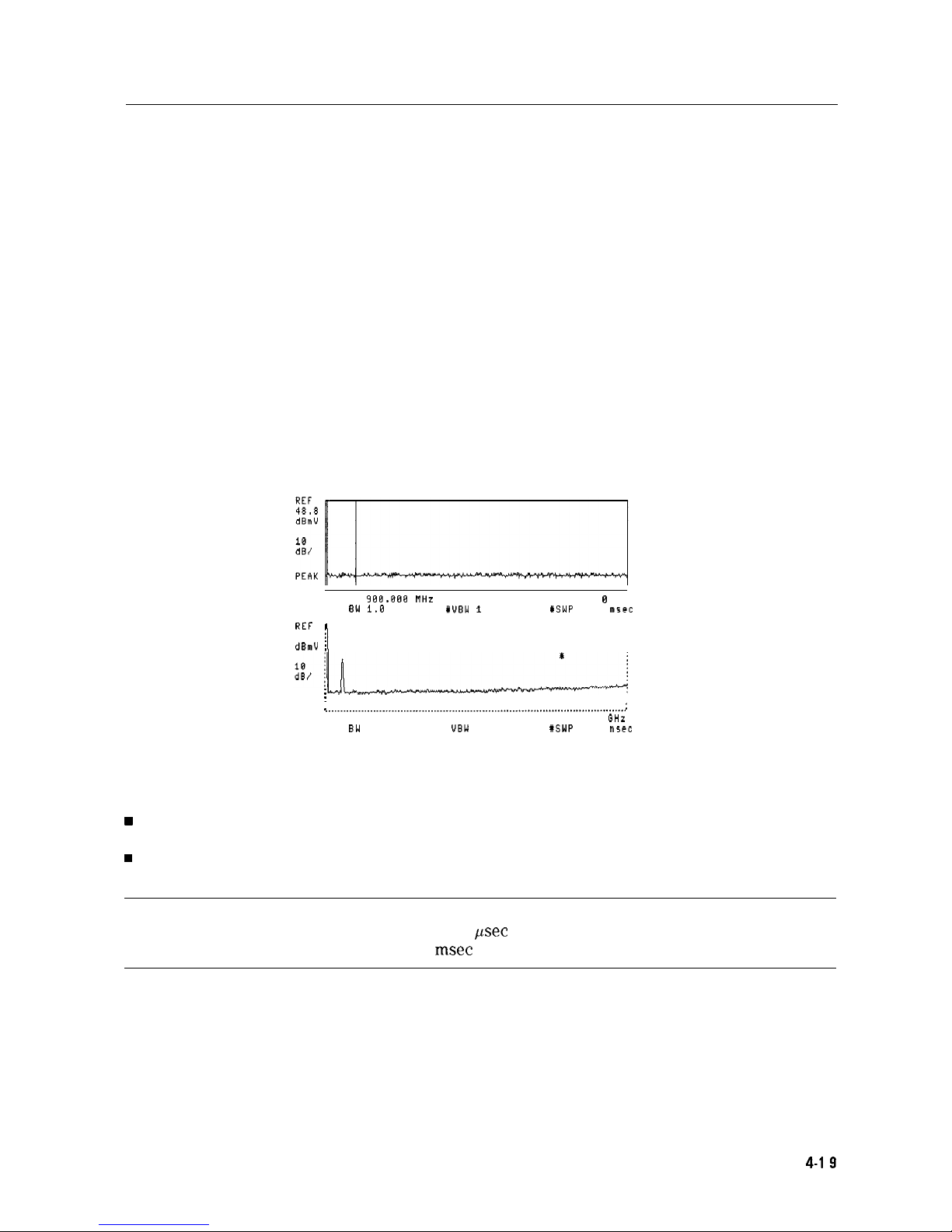
Using the Gate Utility to Simplify Time-Gated Measurements

(Option 105 only)

The time gate allows the user to control when a spectrum analyzer measurement begins and
the length of time during which the measurement is made. The time gate is an RF signal switch
that permits signal into the spectrum analyzer only while the switch, or gate, is closed. Since
the spectrum analyzer receives the signal only when passed through the gate, it will only
display the measurement results from the portion of the signal selected by the time position of
the gate closure. The time gate acts as a time filter, rejecting signals and spectra not occurring
at the desired time.

The time gate utility simplifies the use of the time gate. In the gate utility, the spectrum

analyzer can display the time domain and the frequency domain simultaneously, using two
separate windows. The user is able to adjust the time position of the gate closure relative to
the input signal, using interactive graphic tools in the gate utility. The gate position relative to
the signal is clearly shown in the time domain window. The spectral effects corresponding to
an adjustment of the gate time position are displayed in the frequency domain window. Tools
are provided to aid the user in determining the best gate position, and optimizing the spectrum
analyzer settings for the input signal.

CENTER

980.888

WHz

SPAN B HZ

YRES BW 1.0 MHz YUBW 1 MHz YSWP 18.8

rn5ec

REF

48.8

:
I

dBmV

/

PERK

j

I __..................................................................................................

:

CENTER 900 MHz SPAN 1.800 GHz
RES BW 3.0 MHz

UBW

1 MHz

#SWP 36.8 msec

Figure 4-17. Time-Gate Utility Display

Gate utility features include:

w

Displays time and frequency domains simultaneously.

n Measures continuously.

Interactively controls and displays the gate’s position in time.

n

Note

Option 105, time gate, is required. Option 101, fast ADC, is recommended

psec

(Sweep times down to 20

msec

are available without Option 101.)

The gate utility provides tools to make pulsed RF measurements easy. If the user enters the
optimize the resolution bandwidth, sweep time, and video bandwidth for these pulse

parameters. Coupling the spectrum analyzer settings to pulse characteristics allows easy,

Making Measurements

4-l 9

The types of signals that can be measured using the time gate function include:

n Pulsed RF signals
n Time domain multiple access (TDMA) communication system signals
n Interleaved or intermittent signals
n Signals with transient spectra

Time critical signals are present in many different applications. A few of the applications are
listed below:

n Digital cellular communication systems require measurements on pulse modulated TDMA

signals. Measurements must be accurately aligned with the time division multiple access
(TDMA) burst of the communication carrier. The time gate can position spectrum analyzer
measurement to assess TDMA burst timing and the quality of the burst modulation.

n Rotating head devices, such as VCRs and hard disks, have time interleaved signals

multiplexed from alternate recording tracks on the storage media. The time gate can isolate
the spectrum due to a single recording track.

n Tests required for mobile communication systems often require that the transient spectrum,

due to pulse modulation, be excluded from measurement results.

Example: Measure a Pulsed RF signal.

1. The rear panel GATE OUTPUT must be connected to EXT TRIG INPUT.

2. A TTL trigger signal must be connected to GATE TRIGGER INPUT on the rear panel. If no
trigger is present an error message is displayed and the gate utility will not be activated.

3. Press

[PRESET].

Connect a pulsed RF signal to the spectrum analyzer INPUT 503.

4. Press

(FREQUENCY)

and enter the frequency of your input signal to place the signal at the

spectrum analyzer center frequency.

5.

Press

@iEiTEFj,

CPEAK SEARCH),

[MKR--I)

and MARKER

-+REF

LVL to bring the signal to the

top of the display.

6.

Access the gate utility by pressing [SWEEP], Gate Control , and GATE UTILITY .

Note

If the gate menus are exited without turning the gate utility off (by pressing

another front panel key), press the

(-1

key twice to return to the last gate

utility menu used.

7. Press Define Time to set up the time domain window (the upper window.) Change the
sweep time using the T WINDOW SWP TIME

softkey

so that the pulses are displayed. Press

SWEEP DELAY and use the knob to center the pulses in the upper window.

8. The trigger marker reads out the time from the rear panel gate trigger point to the current
marker position. Turn the trigger marker on by pressing TRIG MKR ON OFF (ON) and
use the knob to move the trigger marker to the edge of the pulse. The marker readout

indicates the position of the edge relative to the rear panel trigger. The trigger marker may
be used to perform “settling time” measurements on the rising or falling edges of a digital
communications signal. (Settling time is the time from the trigger to 90 percent of the
stable pulse on/off value.)

9.

Press Main Menu to exit the define time menu.

4-20 Making Measurements

lo.

Press Define Gate. Use the GATE DELAY and GATE LENGTH keys to position the gate.

Once gate delay or gate length are activated, use the knob and data entry keys can be used
to position the two vertical gate markers. Select a time interval within the last half of the
pulse is selected.

11. Turn the gate on by pressing GATE ON OFF so that ON is underlined. This activates the
frequency domain window, which is the lower window. The spectrum selected with
the current gate position can now be viewed in the frequency domain window. Press

Main Menu.

12. The resolution bandwidth, video bandwidth, and sweep time are not optimized, so the
frequency display may not look correct. There may be signal dropouts or poor frequency
resolution. This can be corrected by entering the pulse parameters and turning on the
coupling.

The gate utility can optimize the setting of resolution bandwidth if the user enters the

value of the pulse width and turns on the coupling. The video bandwidth will be optimized
if the gate length is entered and coupled. The sweep time is optimized when the pulse
repetition interval is entered and coupled.

Press Define

Coupling .

Then press Pulse

Param

to enter the pulse parameters. (This

activates the time domain window and turns off the time gate.) If pulse parameters have

previously been entered, the values will be displayed.

12.

Use the ENTER REF EDGE, ENTER WIDTH, and ENTER PRI

softkeys

to enter the pulse
parameters. These parameter entry tools allow pulse parameters to be entered using a
marker or through the keypad. Press Previous Menu to return to the coupling menu.

14.

Press CPL RBW ON OFF (ON) to turn on the resolution bandwidth coupling. Press

CPL VBW ON OFF (ON), and CPL SWP ON OFF (ON) to turn on the video bandwidth and

sweep time coupling.

15.

Press Main Menu and look at the signal in the time domain window.

16.

Press UPDATE

TIMEFREIJ

so that FREQ is underlined or press

mEXT),

to activate the

frequency window instead of the time domain window. (If the gate was not on when
the user left the frequency window, it may be necessary to press Define Gate and

GATE ON OFF (ON) to turn the gate on again.)

Note

another front panel key), press the key twice to return to the last gate
utility menu used.

Making Measurements

4.21