HP 39gs Graphing Calculator, 40gs Graphing Calculator User Manual

Download

hp 39gs and hp 40gs graphing calculators

Mastering the hp 39gs & hp 40gs

A guide for teachers, students and other users of the hp 39gs & hp 40gs

Edition 1.0

HP part number F2224-90010

Notice

THIS MANUAL AND ANY EXAMPLES CONTAINED HEREIN ARE PROVIDED "AS IS" AND ARE SUBJECT TO CHANGE WITHOUT NOTICE. HEWLETT-PACKARD COMPANY MAKES NO WARRANTY OF ANY KIND WITH REGARD TO THIS MANUAL, INCLUDING, BUT NOT LIMITED TO, THE IMPLIED WARRANTIES OF MERCHANTABILITY, NON-INFRINGEMENT AND FITNESS FOR A PARTICULAR PURPOSE.

HEWLETT-PACKARD CO. SHALL NOT BE LIABLE FOR ANY ERRORS OR FOR INCIDENTAL OR CONSEQUENTIAL DAMAGES IN CONNECTION WITH THE FURNISHING, PERFORMANCE, OR USE OF THIS MANUAL OR THE EXAMPLES CONTAINED HEREIN.

Reproduction, adaptation, or translation of this manual is prohibited without prior written permission of Hewlett-Packard Company, except as allowed under the copyright laws.

Hewlett-Packard Company

16399 West Bernardo Drive, MS 8-600

San Diego, CA 92123

USA

Acknowledgements

Hewlett-Packard would like to thank the author Colin Croft.

Printing History Edition 1 December 2006

Table of Contents

Introduction .......................................................................................................................7

Getting Started ..................................................................................................................9

Some Keyboard Examples ...............................................................................................10

Keys & Notation Conventions ..........................................................................................11

Everything revolves around Aplets! .................................................................................14

The HOME view ...............................................................................................................18

What is the HOME view? .............................................................................................18

Exploring the keyboard ...............................................................................................19

Angle and Numeric settings .........................................................................................28

Memory Management .................................................................................................30

Fractions on the hp 39gs and hp 40gs .........................................................................33

The HOME History .......................................................................................................37

Storing and Retrieving Memories .................................................................................39

Referring to other aplets from the HOME view.............................................................40

A brief introduction to the MATH Menu ........................................................................41

Resetting the calculator................................................................................................42

Summary ....................................................................................................................45

The Function Aplet ...........................................................................................................46

Auto Scale ...................................................................................................................49

The PLOT SETUP view...................................................................................................50

The default axis settings ..............................................................................................52

The Bar ............................................................................................................52

The Menu Bar functions ...............................................................................................53

The FCN menu .............................................................................................................57

The Expert: Working with Functions Effectively ................................................................62

The VIEWS menu..............................................................................................................85

Downloaded Aplets from the Internet ..........................................................................91

The Parametric Aplet .......................................................................................................92

The Expert: Vector Functions ............................................................................................95

Fun and games............................................................................................................95

Vectors ........................................................................................................................96

The Polar Aplet................................................................................................................98

The Sequence Aplet..........................................................................................................99

The Expert: Sequences & Series......................................................................................102

The Solve Aplet..............................................................................................................105

The Expert: Examples for Solve......................................................................................113

The Statistics Aplet - Univariate Data..............................................................................114

The Expert: Simulations & random numbers...................................................................120

The Statistics Aplet - Bivariate Data................................................................................123

The Expert: Manipulating columns & eqns......................................................................133

The Inference Aplet ........................................................................................................141

The Expert: Chi2 tests & Frequency tables .......................................................................147

The Linear Solver Aplet ..................................................................................................150

Example 1 .................................................................................................................150

Example 2 .................................................................................................................150

Example 3 .................................................................................................................151

The Triangle Solve Aplet ................................................................................................152

Example 1 .................................................................................................................152

Example 2 .................................................................................................................153

Example 3 .................................................................................................................154

The Finance Aplet ..........................................................................................................155

The Quad Explorer Teaching Aplet .................................................................................159

The Trig Explorer Teaching Aplet....................................................................................162

The MATH menus...........................................................................................................165

Accessing the MATH menu commands........................................................................166

The PHYS menu commands........................................................................................168

The MATH menu commands.......................................................................................169

The ‘Real’ group of functions .....................................................................................170

The ‘Stat-Two’ group of functions ..............................................................................178

The ‘Symbolic’ group of functions ..............................................................................179

The ‘Tests’ group of functions ....................................................................................182

The ‘Trigonometric’ & ‘Hyperbolic’ groups of functions ..............................................182

The ‘Calculus’ group of functions ...............................................................................184

The ‘Complex’ group of functions ..............................................................................186

The ‘Constant’ group of functions ..............................................................................189

The ‘Convert’ group of functions ...............................................................................189

The ‘List’ group of functions .......................................................................................190

The ‘Loop’ group of functions ....................................................................................193

The ‘Matrix’ group of functions..................................................................................195

The ‘Polynomial’ group of functions...........................................................................202

The ‘Probability’ group of functions ...........................................................................205

Working with Matrices ..................................................................................................209

Working with Lists.........................................................................................................215

Working with Notes & the Notepad...............................................................................217

Independent Notes and the Notepad Catalog ............................................................219

Creating a Note .........................................................................................................220

Working with Sketches..................................................................................................222

The DRAW menu........................................................................................................223

Copying & Creating aplets on the calculator...................................................................226

Different models use different methods to communicate.............................................227

Sending/Receiving via the infra-red link or cable.......................................................228

Creating a copy of a Standard aplet. .........................................................................230

Some examples of saved aplets ................................................................................232

Storing aplets & notes to the PC.....................................................................................237

Overview ..................................................................................................................237

Software is required to link to a PC ...........................................................................238

Sending from calculator to PC ....................................................................................239

Receiving from PC to calculator..................................................................................244

Aplets from the Internet.................................................................................................245

Using downloaded aplets ..........................................................................................249

Deleting downloaded aplets from the calculator ........................................................250

Capturing screens using the Connectivity Kit ..............................................................251

Editing Notes using the Connectivity Software................................................................252

Programming the hp 39gs & hp 40gs ............................................................................255

The design process ....................................................................................................255

Planning the VIEWS menu .........................................................................................257

The SETVIEWS command ............................................................................................259

Example aplet #1 – Displaying info............................................................................262

Example aplet #2 – The Transformer Aplet.................................................................268

Designing aplets on a PC ...........................................................................................270

Example aplet #3 – Transformer revisited ..................................................................272

Example aplet #4 – The Linear Explorer aplet ............................................................274

Alternatives to HP Basic Programming...........................................................................281

Flash ROM.....................................................................................................................284

Programming Commands ..............................................................................................286

The Aplet commands .................................................................................................286

The Branch commands...............................................................................................287

The Drawing commands ............................................................................................289

The Graphics commands ............................................................................................291

The Loop commands ..................................................................................................291

The Matrix commands ...............................................................................................292

The Print commands ..................................................................................................293

The Prompt commands ..............................................................................................294

Appendix A: Some Worked Examples............................................................................298

Finding the intercepts of a quadratic ..........................................................................298

Finding complex solutions to a complex equation ......................................................299

Finding critical points and graphing a polynomial......................................................300

Solving simultaneous equations.................................................................................302

Expanding polynomials .............................................................................................304

Exponential growth ...................................................................................................305

Solution of matrix equations......................................................................................307

Finding complex roots ...............................................................................................308

Complex Roots on the hp 40gs ..................................................................................309

Analyzing vector motion and collisions ......................................................................310

Circular Motion and the Dot Product ..........................................................................311

Inference testing using the Chi2 test............................................................................312

Appendix B: Teaching or Learning Calculus....................................................................314

Investigating the graphs of y=xn for n an integer ....................................................314

Domains and Composite Functions .............................................................................315

Gradient at a Point ....................................................................................................317

Gradient Function ......................................................................................................318

The Chain Rule...........................................................................................................319

Optimization .............................................................................................................319

Area Under Curves ....................................................................................................320

Fields of Slopes and Curve Families ...........................................................................320

Inequalities................................................................................................................321

Rectilinear Motion......................................................................................................321

Limits.........................................................................................................................321

Piecewise Defined Functions ......................................................................................322

Sequences and Series ................................................................................................322

Transformations of Graphs ........................................................................................323

Appendix C: The CAS on the hp 40gs .............................................................................324

Introduction ...............................................................................................................324

Using the CAS ............................................................................................................327

Examples using the CAS ............................................................................................341

The CAS menus ..........................................................................................................358

On-line help ..............................................................................................................361

Configuring the CAS...................................................................................................362

Tips & Tricks - CAS .....................................................................................................366

NNTTRROODDUUCCTTIIOON

This book is intended to help you to master your hp 39gs or hp 40gs calculator but will also be useful to users of earlier models such as the hp 39g, hp 40g and hp 39g+. These are very sophisticated calculators, having more capabilities than a mainframe computer of the 1970s, so you should not expect to become an expert in one or two sessions. However, if you persevere you will gain efficiency and confidence.

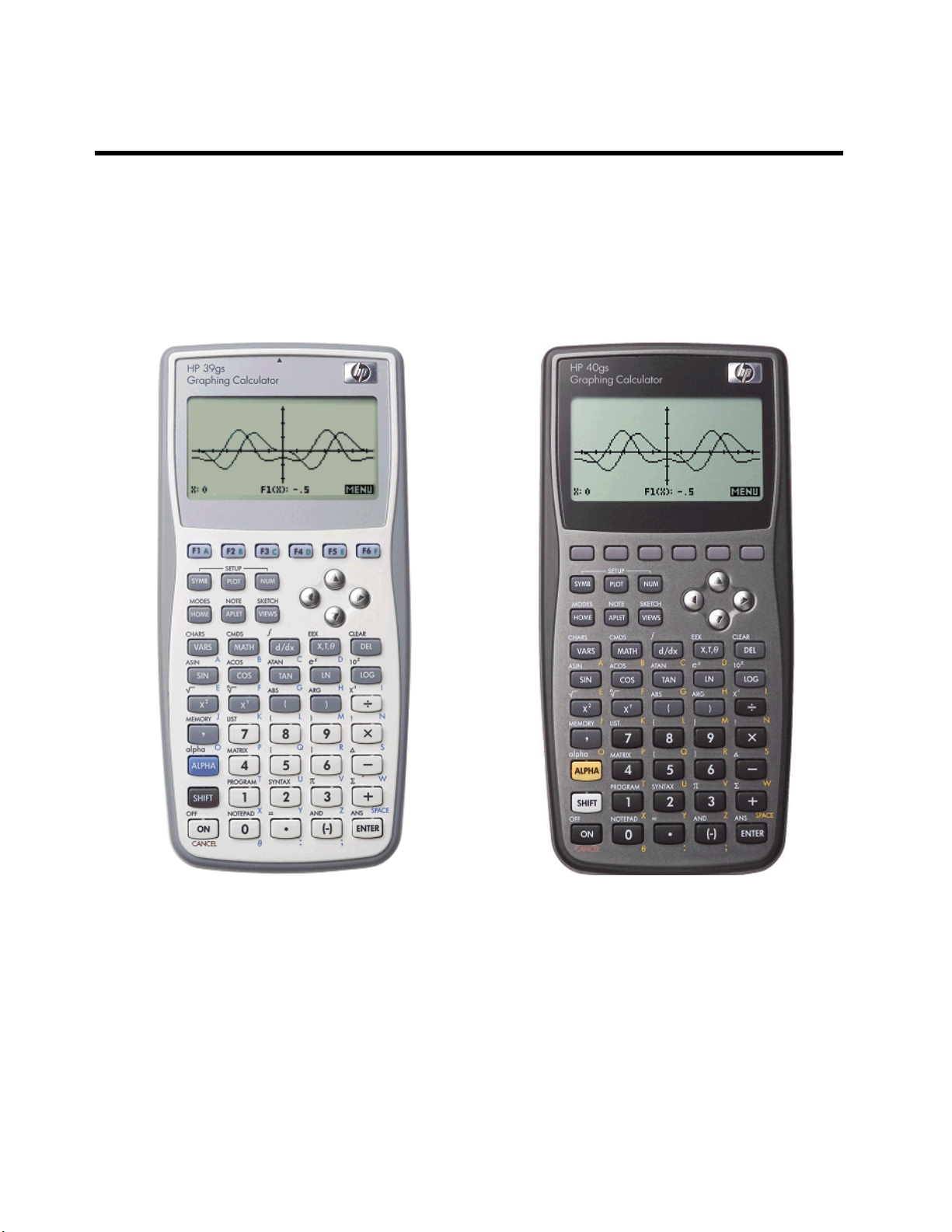
The hp 39gs vs. the hp 40gs

The hp 39gs and hp 40gs, shown above, are ‘sister’ calculators released in 2006. They are identical in almost all respects except for their color schemes and in whether they have infra-red or a CAS. The hp 39gs was released mainly in the United States and other regions, such as Australia, which do not allow a Computer Algebra System, or CAS, in their educational systems. The hp 40gs, on the other hand, was released mainly in Europe where a CAS has long been an expected ability for calculators used by high school students. The hp 39gs has infra-red communication, similar to that of a TV remote control, which allows easy transmission of programs and aplets between calculators. The hp 40gs does not and uses a cable instead.

Many of the markets targeted by the hp 40gs do not allow infra-red communication in assessments and so, on the hp 40gs, this ability is permanently disabled, substituting instead a mini-serial cable supplied with the calculator (see page 237). The previous models, the hp 39g & hp 40g shared a common chip and, although it was never intended to be possible, a hacker released a special aplet for the hp 39g which would ‘convert’ it into an hp 40g and activate the CAS. This is not the case with the hp 39gs & hp 40gs: the internal chips are different and there is no way to ‘convert’ one into the other using an aplet or program.

For more information on the CAS, see page 324. This manual will cover, for the most part, the features which are shared by both calculators with the CAS covered in Appendix C. A detailed manual for the CAS is also supplied with the hp 40gs and more information can be found on the official HP website and on the author’s website The HP HOME view at

http://www.hphomeview.com

The majority of readers of this manual may only have used a Scientific calculator before so explanations are as complete as possible. However it is not the purpose of this book to teach mathematics and knowledge will largely be assumed. Those already familiar with another brand or type of calculator may find a quick skim sufficient, concentrating perhaps on the ‘Expert User’ chapters.

This book provides a supplement to the official manual and, more importantly, expert tips to make your work smother and more confident. It has been designed to cover the full use of the hp 39gs and hp 40gs calculators. This means explanations which will be useful to anyone from a student who is just beginning to use algebra seriously, to one who is coming to grips with advanced calculus, and also to a teacher who is already familiar with some other brand of graphic calculator.

The impact graphical calculators are having on the topics taught and even more, the way they are taught is proving to be profound. The inventiveness and flexibility of teachers of mathematics is being stretched to the limit as we gradually change the face of teaching in the light of these machines. For those concerned with the impact of a graphical calculator on the ‘fundamentals’ of mathematics, it should be recalled that the same fears were held for scientific calculators when they were introduced to schools. History has shown that these fears were generally groundless. Students are learning topics in high school that their parents did not cover until university years. In particular, the scientific calculator proved to be a great boon to students of middle to lower ability in mathematics, relieving them of the burden of tedious calculations and allowing them to concentrate on the concepts. It is my opinion, as a practicing mathematics teacher of some 25 years, that this is also the case with graphical calculators.

EETTTTIINNG

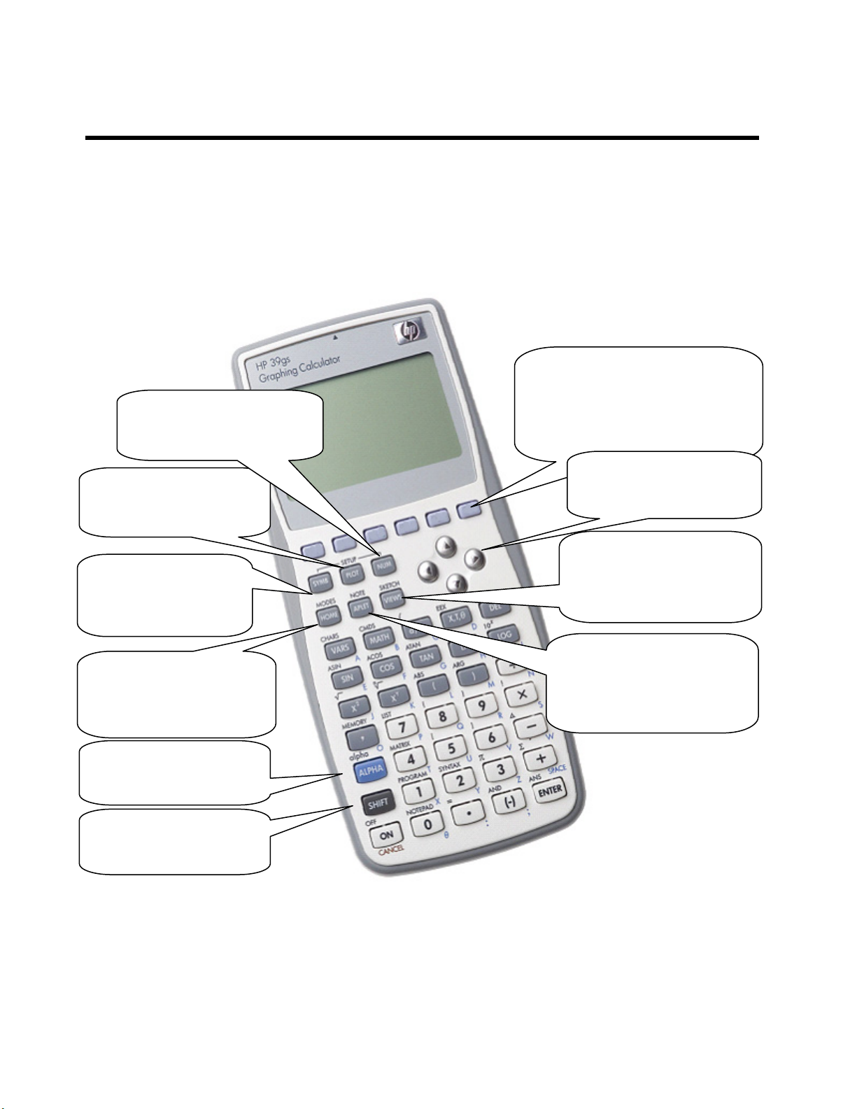
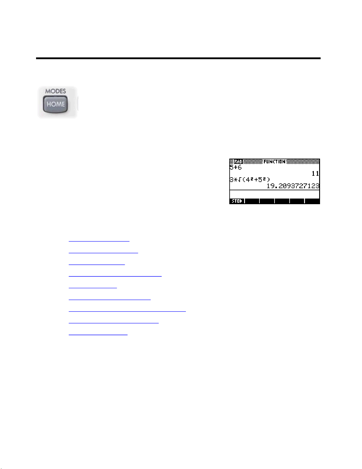
Let’s begin by looking at the fundamentals - the layout of the keyboard and the positions of the important keys used frequently. The sketch below shows most of the important keys. As can be seen on the previous pages, the keyboards for the hp 39gs and hp 40gs are exactly the same except for the different color schemes. These keys are the ones which control the operation of the calculator – most others are simply used to do calculations once the important keys have set up the environment to do it in.

The NUM key gives you a tabular view of your function, sequence or data.

The PLOT key displays the graph view for any given environment.

The SYMB key nearly always takes you to a view in which you can enter e

uations.

TTAARRTTEED

These six screen keys change their function in different contexts. The bar at the bottom of the screen labels them. Check this bar for special functions in any given context.

These are the arrow keys. They let you move within a screen.

The VIEWS key gives a different menu in each aplet. It can be very useful, and is always worth checking.

HOME is where you will do most of your calculations. It is shared by all the aplets and oversees them all.

The ALPHA key accesses the alphabetical chars below most buttons.

The SHIFT key accesses the extra functions above most buttons.

The APLET key is central. This key allows you to choose which mathematical environment you wish to work in.

Examples of the effects of each of these keys and many more are shown on the pages that follow.

OOMME

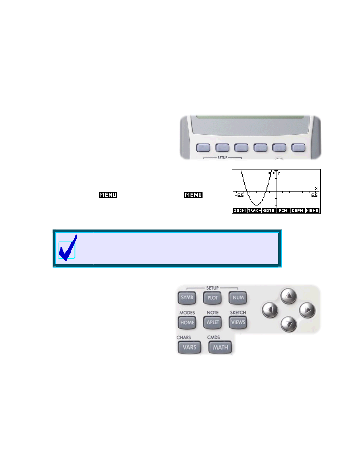
Shown below are snapshots of some typical screens (called “views”) which you might see when you press the keys shown on the previous page. Exactly what you see depends on which aplet is active at the time. See page

The Function aplet is used below to illustrate this. The normal use of the Function aplet is to graph and analyze Cartesian functions. Notice at the bottom of the various screens how the meanings of the row of unlabelled screen keys change in different views.

EEYYBBOOAARRD

14 for an introduction to aplets.

SYMB key - in this case it is set to graph

The

the function

XXAAMMPPLLEES

= x − x2 − 7 x + 6 .x

()

PLOT key - used to graph the function.

The

PLOT SETUP view sets the axes.)

(The

The NUM key showing a tabular view of the function.

NUM SETUP view sets table parameters.)

(The

The

APLET key is used to choose which aplet is active. There are 12

aplets provided with the calculator and more can be downloaded from the internet.

The MATH key gives access to more than a hundred extra functions, grouped into categories. The view shown right is part of the Probability section.

There are a number of types of keys/buttons that are used on the hp 39gs and hp 40gs.

The basic keys are those that you see on any calculator including scientific ones, such as the numeric operators and the trig keys. Most of these keys have two or more functions, with the second function accessed via the

In this book, all references to buttons, whether they need the

KEY.

The SHIFT and ALPHA keys

EEYYS

SHIFT key and the alphabetic character accessed via the ALPHA key.

&&N

OOTTAATTIIOON

OONNVVEENNTTIIOONNS

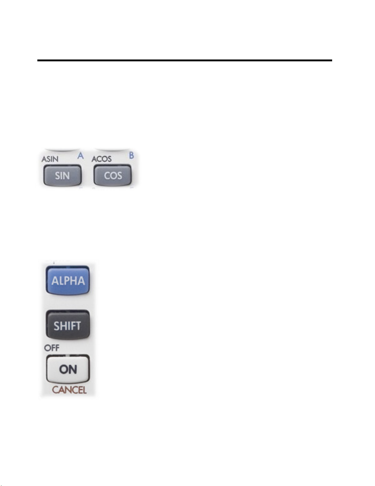
Take for example the you get the right you will see two additional meanings assigned via the

ALPHA keys.

and

COS function. However above left of the key and below

COS key shown left. If you just press the key,

SHIFT key or not, are written in this typeface:

SHIFT

SHIFT key gives you the second function for each key. In the case of the

The

COS key, the second function is ACOS, sometimes referred to as arc-cos or cos

or inverse cos. Most keys have these second functions that are obtained via the

SHIFT key.

Note: When I want you to use one of these keys that needs to have the key pressed first I usually won’t say so. It seems to me that you’re intelligent enough to work out for yourself when the

The ALPHA key

The next modifier key is the characters, and these appear below and right of most keys. Pressing before the the calculator can be locked in can also simply hold down the

ALPHA key will give lower case alphabetic characters. In many views

ALPHA key. This is used to type alphabetic

ALPHA mode using one of the screen keys. You

ALPHA key.

SHIFT key needs to be pressed.

SHIFT

-1

The Screen keys

A special type of key unique to the hp 39gs, hp 40gs and family is the row of blank keys directly under the screen. These keys change their function depending on what you are doing at the time. The easiest way to see this is to press the

APLET key. As you can see right, the functions

are listed at the bottom of the screen. All you have to is to press the key under the screen definition you want to use. These buttons are normally referred to as SK1 to SK6, where SK is “Screen Key”.

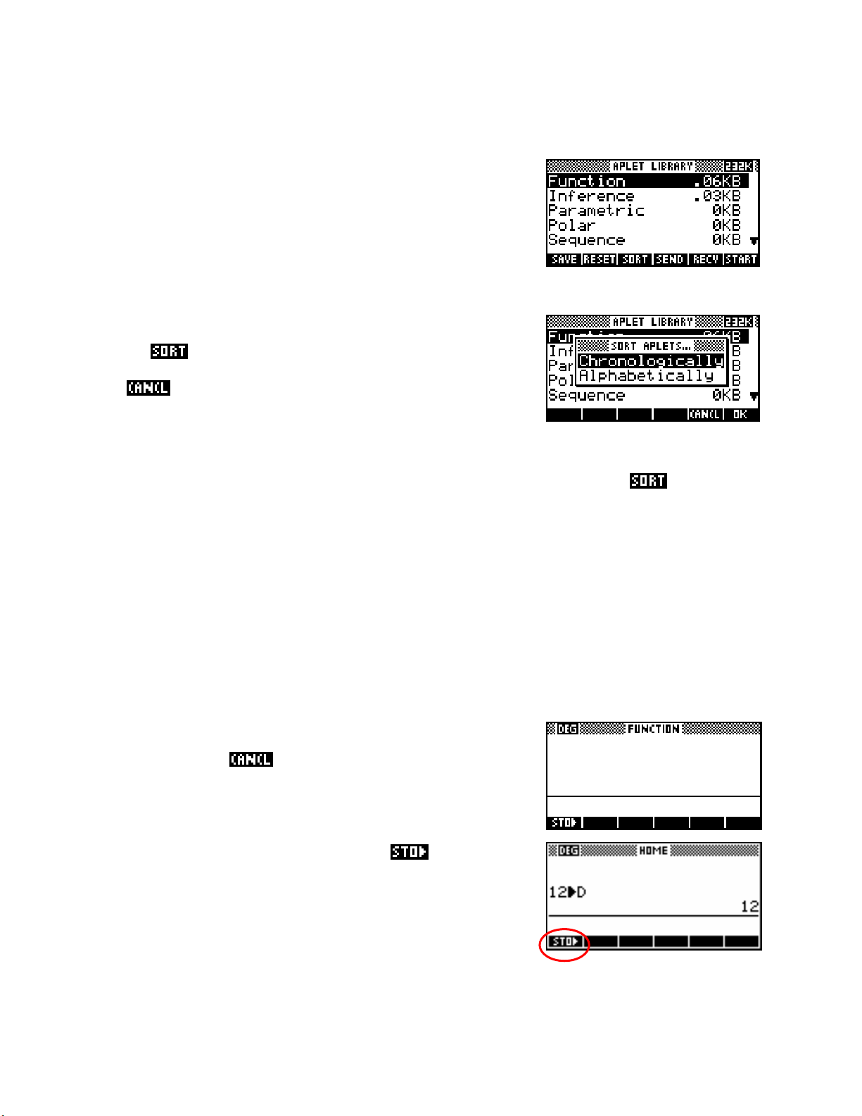
All references to keys of this type are shown as images of the label. For example, if I want you to press the key under the SORT label it would be written as

. Do it now and you’ll see the screen shown on the right. Notice that the keys have now changed function. Press the one under

to return to the previous view.

Pop-up menus & short-cuts

Sometimes pressing a key pops up a menu on the screen as you just saw. You use the up/down arrow keys to move the highlight through the menu and make choices by pressing the listed in a menu will usually be written using italics. As an example, I might say to press

ENTER key. Choices that are

and choose

Chronologically. The manual you are given with your calculator uses a different convention.

As mentioned before, the third way a key can be used is to get letters of the alphabet. This is not so that you can write letters to your friends (although you can do that with the Notepad) but so that you can use variables like X and Y or A and B. The key above the alphabet. Lower case letters are obtained by pressing the type in more than just a single letter, hold down the

SHIFT key labeled ALPHA is used to type in letters of the

SHIFT key before the ALPHA key. If you want to

ALPHA key. Unfortunately, this doesn't work for

lowercase.

Try this…

If you haven’t already, Press the

HOME key to see the screen on the right. Yours may not be

out of the menu from the previous screen.

blank like mine but that doesn’t matter.

1 2 and then press the screen key labeled , circled on the

Press image. Now press the

XTθ key). Finally, press the ENTER key. Your screen should look

the like the one on the right. You have now stored the value

D. Each alpha key can be used as a memory.

Note that memories

ALPHA key and then the alphabetic D key (on

12 into memory

X, T and θ are regularly overwritten by the normal

operation of the calculator and should be used with caution.

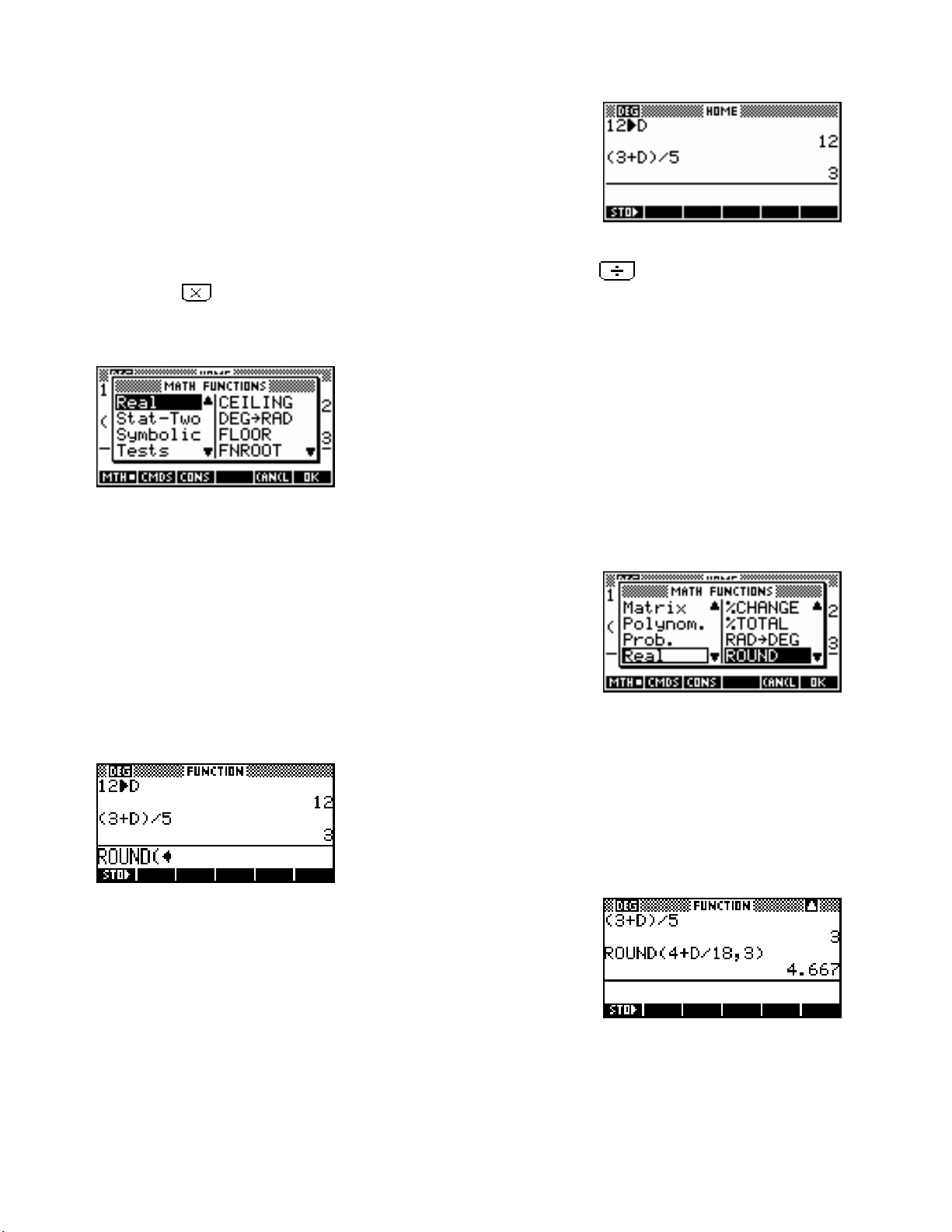
You can also use these memories in calculations. Type in the following, not forgetting the

ALPHA key before the D….

(3+D)/5 ENTER

The calculator will use the value of haven’t worked it out for yourself, the multiply key

12 stored earlier in D to evaluate the expression (see image). In case you

/ symbol comes from the divide key and the * symbol from the

More information on memories and detailed information on the HOME view in general is given on pages 39.

The calculator also comes with an immense number of mathematical functions. They can all be obtained via menus through the from the keyboard. Try pressing the

MATH key now and you should

MATH key or

find your screen looks like the screen shot left.

MATH menu is covered in detail on pages 165 but we will have a brief look now.

The

The left side of the menu lists the categories of functions. As you use the up/down arrows to scroll through the topics, you’ll see the actual list on the right change. Move down through the menu until you reach Prob. (short for Probability) and then one step more and you’ll find yourself back at Real. Now press the right arrow key and your highlight will move into the right hand menu (see above). Move the highlight down through this menu until you reach Round. Press

ENTER.

You should now be back the display as shown right. You can also achieve the same effect by

ALPHA to type in the word letter by letter. Many people prefer to

using do it that way.

Now type in:

4+D/18,3) and press ENTER

As you can see, the effect was to round off the answer of 4 3 decimal places. Entering

ROUND(4+D/18,-3) would have rounded to

3 significant figures instead.

There are shortcuts for obtaining things from the

MATH menu that are

covered later (see page 41).

HOME, with the function ROUND( entered in

666666.. to

VVEERRYYTTHHIINNGGRREEVVOOLLVVEESSAARROOUUNND

A built in set of aplets are provided in the and hp 40gs. This effectively mean that it is not just one calculator but a dozen (or more), changing capabilities according to which aplet is chosen.

The best way to think of these aplets is as “environments” or “rooms” within which you can work. Although these environments may seem dissimilar at first, they all have things in common, such as that the produces graphs, that the

NUM key displays the information in tabular form.

There are twelve standard aplets available via the the Internet (see pages 255 & 245). These aplets are:

SYMB key puts you into a screen used to enter equations and rules, and that the

APLET view on the hp 39gs

APLET key. More can be created by you or obtained via

PPLLEETTS

PLOT key

The Finance aplet (see page 155)

Performs calculations involving time/value of money.

The Function aplet (see page 46)

Provides f(x) style graphs, calculus functions etc. It will not only graph but find intercepts, intersections, areas and turning points.

The Inference aplet (see page 141)

Allows the investigation of inferential statistics via hypothesis testing and confidence intervals.

The Linear Solver aplet (see page 150 )

This aplet is used to solve simultaneous linear equations in two or three unknowns.

The Parametric aplet (see page 92)

Handles x(t), y(t) style graphs. Can also be used to help with vector motion.

The Polar aplet (see page 98)

Handles r(θ) style graphs. Quite apart from their mathematical use, they produce some really lovely patterns!

The Quadratic Explorer aplet (see page 159)

This is a teaching aplet, allowing the student to investigate the properties of quadratic graphs using an interactive format which allows the connection between the coefficients and the graph to be easily seen.

The Sequence aplet (see page 99)

(

Handles sequences such as T

recursive and non-recursive sequences.

+ 3; T1 = 2 or T = 2

n−1

The Solve aplet (see page 105)

n−1

. Allows you to explore

Solves equations for you. Given an equation such as A

variable if you tell it the values of the others.

2πr r + h

it will solve for any

)

The Statistics aplet (see page 114 & 123)

Handles descriptive statistics. Data entry is easy, as is editing. It analyzes univariate and bivariate data, drawing scatter graphs, histograms and box & whisker graphs and finding lines of best fit, linear and non-linear.

The Triangle Solve aplet (see page 152 )

This aplet solves for sides and angles in triangles.

The Trig Explorer aplet (see page 162)

This is a teaching aplet, allowing the student to investigate the properties of sine and cosine graphs in the same interactive fashion as the Quadratic Explorer.

The Function aplet is probably the easiest to understand and also the one you will use most often, so we will have a very quick look at the commonly seen views of this aplet.

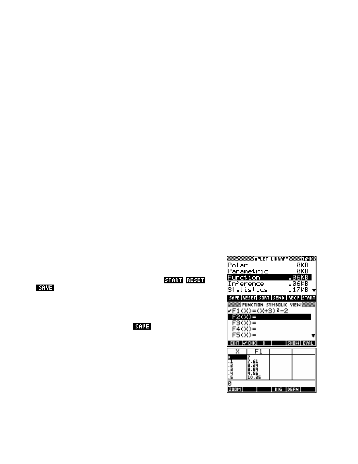
Some typical aplet views

APLET key is used to list all the aplets and to , or

The

them.

SYMB view is used to enter equations….

The It can store up to ten functions. If you copies of the aplet then any number of functions can be used.

NUM view shows the function in table form…

The

additional

The

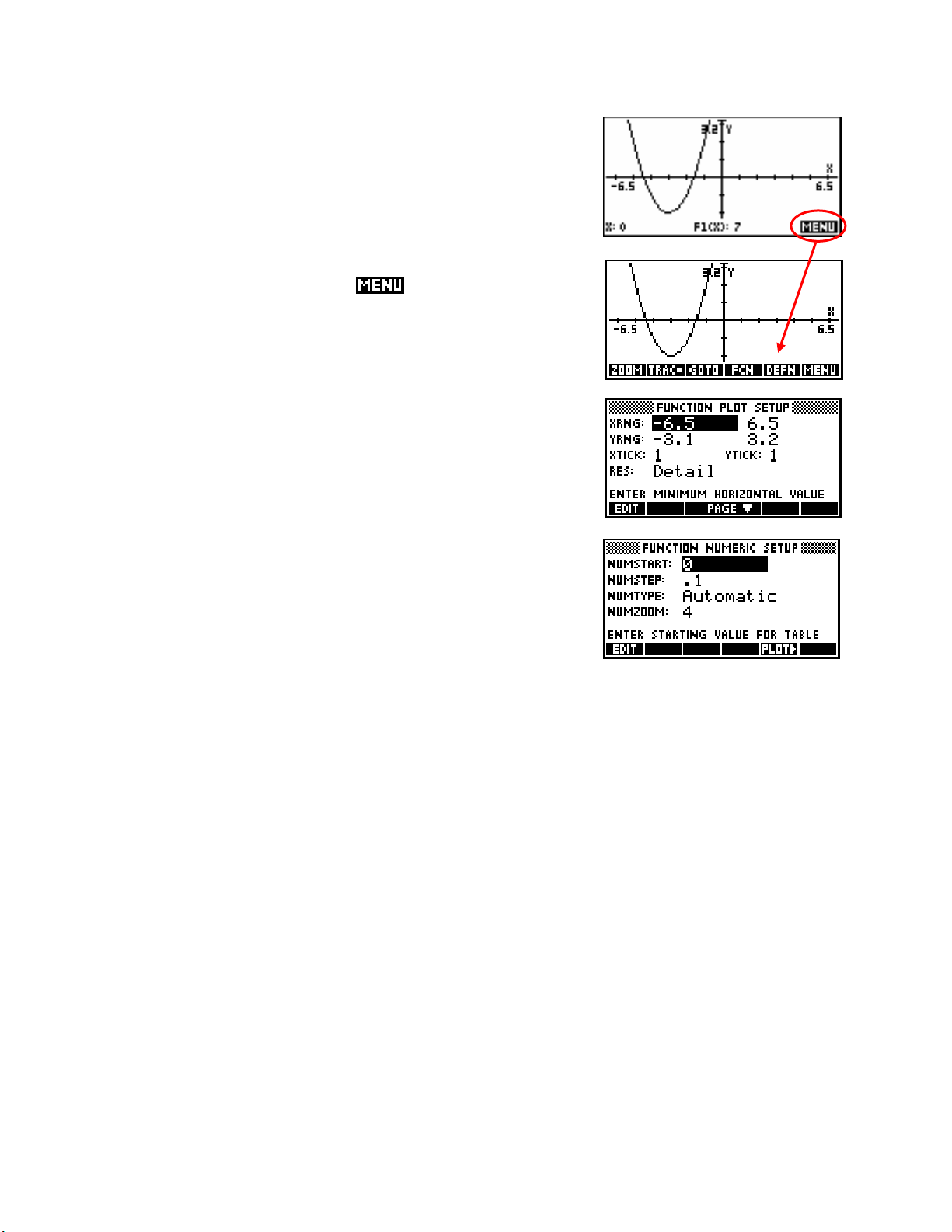
PLOT view is used to display the function as a graph…

At the bottom of the

PLOT view is the

key. This gives access to a number of other useful tools allowing further analysis of the function. Some of these tools have their own sub-menus.

PLOT SETUP view controls the settings for the PLOT view…

The

NUM SETUP view controls the settings for the NUM table view…

The

Although these views are superficially different in other aplets, the basic idea is usually similar.

Having said that aplets are best thought of as “working environments”, it is equally true that aplets are essentially programs, with the standard ones simply being built into the calculator. This is a programmable calculator, having its own programming language and able to perform quite sophisticated tasks.

Unless you particularly want to learn about the programming language, there is no reason why you should worry about it. The standard aplets will cover all of your normal requirements in mathematics.

However one of the great strengths of the hp 39gs and hp 40gs is their ability to “download” additional aplets from other calculators and from the Internet. See page

245.

A mini-USB cable (see page 237) and software were provided with your hp 39gs and hp 40gs which you

A g

can use to connect your PC to your calculator via the USB port and then download aplets from the computer to the calculator or to save your work to the computer. If you have an earlier model such as the hp 38g, hp 39g or hp 40g then you need to buy the cable separately from an HP reseller and download the software from Hewlett-Packard’s website. More information on this can be found on pages 245 - 274.

Calculator Tip

If you search on the web using the key words “39g” or “40g” and you will find a variety of sites which contain information and aplets. lar

e variety of programs and aplets were written for the older hp 39g & hp 40g and these will generally run with no problems on the hp 39gs & hp 40gs. www.hphomeview.com) has the largest

The author’s site (

collection and has extensive help pages as well.

Once an aplet is transferred onto any calculator from the PC, transferring it to another takes only seconds using the built in infra-red link at the top of each calculator on the hp 39gs or using the mini-serial cable on the hp 40gs. The infra-red link is exactly like the remote control of a TV or VCR, and allows two calculators to talk to each other. In the interests of security in examinations the distance over which the infra-red link can communicate is limited to about 8 - 10cm (about 3 - 4 inches). See page

237 for details on this process. The hp 40gs does not have infra-red because some of the markets for which it was produced did not wish students to have this capability.

Aplets are available to do many mathematical tasks such as statistical simulations, time series analysis as well as many tasks called for in calculus, physics and chemistry. There are a number of sites which offer aplets.

The Hewlett-Packard site is found at…

http://www.hp.com/calculators

(follow the links to graphical calculators and then your model)

In addition to this you should check the site called The HP HOME view which can be found at…

http://www.hphomeview.com

(This site is maintained by the author and contains not only hundreds of aplets and games, but also a huge amount of detailed information on the 39gs/40gs family of calculators.)

The entire topic of aplets is discussed in more detail in the chapter entitled “Copying & creating aplets” on page

226.

Calculator Tip

The aplets for an hp 39/40 family are interchangeab e but those of an hp 38g are not.

If you load an aplet from an hp 38g onto an newer

model then the download may appear to be successfu but the

calcu ator will “crash” when the aplet is run. No permanent damage

will be done but it may cause a reset with loss of user information. Programs from the hp 48 and 49 family are not compatible with those of the 39/40 family (nor vice versa).

HHE

HHOOMME

In addition to the aplets, there is also the scratch pad for all the others. This is accessed via the you will do your routine calculations such as working out 5% of $85, or finding √35. The

HOME view is the view that you will most often use, so we will explore that view first.

WWhhaattiisstthheeHHOOMMEEvviieeww?

This is the accessed from it and can affect it to varying degrees. All mathematical functions are available in this view. You should learn to use this view as efficiently as possible, since a great deal of work will be done here.

We will explore the

HOME base for the calculator. All other aplets can be

HOME view in the following order:

• Exploring the Keyboard

VVIIEEW

HOME view, which can best be thought of as a

HOME key and is the view in which

• Angle and numeric settings

• Memory management

• Fractions on the hp 39gs & hp 40gs

• The

• Storing and retrieving memories

• Referring to other aplets from the

• An introduction to the

• Resetting the calculator

HOME History

HOME view

MATH menu

EExxpplloorriinnggtthheekkeeyybbooaarrd

The first step in efficient use of the calculator is to familiarize yourself with the mathematical functions available on the keyboard. If we examine them row by row, you will see that they tend to fall into two categories - those which are specific to the use of aplets, and those which are commonly used in mathematical calculations.

The screen keys

The first row of blank keys are context defined. The reason they have no label is that their meaning is redefined in different situations - they are the ‘screen keys’. The current meaning of each key is listed in the row of boxes at the bottom of the screen.

A common abbreviation used for these keys is “screen key 1” ). In the are labeled, such as the row of screen keys labels in the another view where all the keys are in use, change to the

Aplet related keys

The next two rows of keys and part of the third are mainly aplet related, so we’ll deal with them as a group.

The arrow keys

The arrow keys on the right are used in most views, usually to move the cursor (a small cross) or the highlight around on the screen.

PLOT view shown right, some of the screen keys

key. When you press this key the

PLOT view appear or disappear. To see

Calculator Tip

Develop the habit of checking the screen to see if any of those keys have been given meanings. In many views, the screen keys have been set up with useful shortcuts and functions.

SK1 or SK2 etc (for

APLET view.

The

APLET key is used to choose between the various different aplets

available. Everything in the calculator revolves around aplets, which you can think of either as miniature programs or as environments within which you can work.

The hp 39gs and hp 40gs come with twelve standard aplets - Finance, Function, Inference, Parametric, Polar, Linear Solver, Triangle Solver, Quadratic Explorer, Sequence, Solve, Statistics and Trig Explorer. Which one you want to work with is chosen via the page

14 for more details on this.

APLET key. See

Calculator Tip

The name of the active aplet is shown at the top of the screen, as above. It is important to bear this in mind because the angle and numeric settings are tied to the active aplet. Changing aplets may therefore cause these settings to change in

HOME too. See page 28.

In addition to the standard twelve, covered in great detail in the chapters following, many more aplets are available from the Internet written by other programmers. Once these are downloaded into your calculator they can also be accessed via the

APLET key. For more detail on this type of aplet, see the brief summary

later in this section, and the chapter entitled “Programming the hp 39gs & hp 40gs” on page 255.

The SYMB, PLOT and NUM keys

When working mathematically there are three ways that we view functions:

• symbolically, as an equation;

• numerically, as a table;

• graphically, as a graph in various formats.

SYMB, PLOT and NUM keys are intended to reflect this common

The methodology. In most aplets the

SYMB view shows the equations and the NUM view shows the

PLOT view shows the graph, the

equations in tabular (numeric) format.

The VIEWS key pops up a menu from which you can choose various options. Part of the See page

85 for more detailed information. A summary only is given

VIEWS menu for the Function aplet is shown right.

below.

Essentially the

VIEWS menu is provided for two purposes…

Intro to the VIEWS menu

Firstly, within the standard aplets (Function, Sequence, Solve etc.) it provides a list of special views available to enhance the

For example the standard covering the whole screen, but the screen such as shown right. Information on the

PLOT view.

PLOT screen provides a standard graph

VIEWS menu lets you use a split

VIEWS menu is given in

the chapter dealing with the Function aplet.

In its second role, the

VIEWS key also has a critical purpose when using aplets which have been downloaded

from the Internet. When a programmed aplet is created for the hp 39gs or hp 40gs, a menu is provided by the programmer to let you control and use it. During the programming this menu is tied to the

VIEWS key,

replacing the menu normally found on the key.

For example, the snapshot shown right is of a

VIEWS menu taken from

an aplet designed to analyze and graph Time Series data.

The next important key is the

HOME view from wherever you are. Above it is the MODES key,

the accessed by pressing

SHIFT first. More detailed information on these

HOME key. It allows you to change into

two views follows later.

The VARS key

VARS key is used, mainly by programmers, as a compact way to access all the

The different variables stored by the calculator including aplet environment variables.

Shown right are two views of the list showing the graphic variables (memories) from the

PLOT.

The

APLET list showing some of the variables in the set controlling

VARS key is not generally used much, and you may not have

VARS screen, the first from the HOME

G1, G2…. and the next

followed this explanation. This is not important as it is a key that is very rarely used by the average user. A few uses for the average user are detailed in the Function aplet’s “Expert User” section on page 62.

MATH key next to VARS is far more important and provides access to a

The huge library of mathematical functions. The more common functions have keys of their own, but there is a limit to the number of keys that one can put on a calculator before it takes too long to find the key required. Hence the

MATH menu lists all those functions that would not fit onto the

The

MATH key.

keyboard plus some which also appear on the keyboard. Shown in the screen snapshot right is a small selection of the total list. For a listing of almost all the functions, with examples of their use, see the chapter entitled “The MATH Menus” on page 165.

As is usual with all calculators, most of the keys have another function above the key. The hp 39gs and hp 40gs get twice the action from each key by having this second function.

The second function is accessed via the

SHIFT key on the left side of the calculator. Although this book will

sometimes tell you explicitly to press this key, in most cases it will be assumed that you are intelligent enough to work out for yourself when it is necessary to press it.

The

ALPHA key gives access to the alphabetical characters, shown below and

right of most keys. Pressing

SHIFT ALPHA gives lower case.

Calculator Tip

If you press and hold down the key you can ‘lock’ alpha mode,

ALPHA

although this doesn’t work for lower case. Many people use this to type in functions by hand rather than going through the views, such as the Notepad, also offer a screen key function that lets you lock either upper or lower case alpha mode.

The SETUP views

SETUP views, above PLOT, SYMB and NUM, are used to customize

The their respective views. For example, the

PLOT SETUP screen controls things

like axes, labels etc. Their use changes in different aplets, so for more information see the explanations in the chapters dealing with the various aplets, particularly in the Function aplet on page

50.

MATH

menu. Some

SYMB SETUP key is only used in one place, which is to choose the data model for bivariate statistics in

The the Statistics aplet. It is not available in the other aplets and trying to access it will result only in a quick flash of an exclamation mark on the screen to say “You’ve done something wrong!”.

Information on the use of the

VIEWS keys) can be found in the chapters “Working with Sketches” and

and

SKETCH and NOTE views (located above the APLET

“Working with Notes & the Notepad” on pages 222 & 217.

The main use for the

SKETCH and NOTE views is in aplets downloaded from the Internet. Instructions for

using the aplet are sometimes included with the aplet in note form, and sometimes as an accompanying sketch.

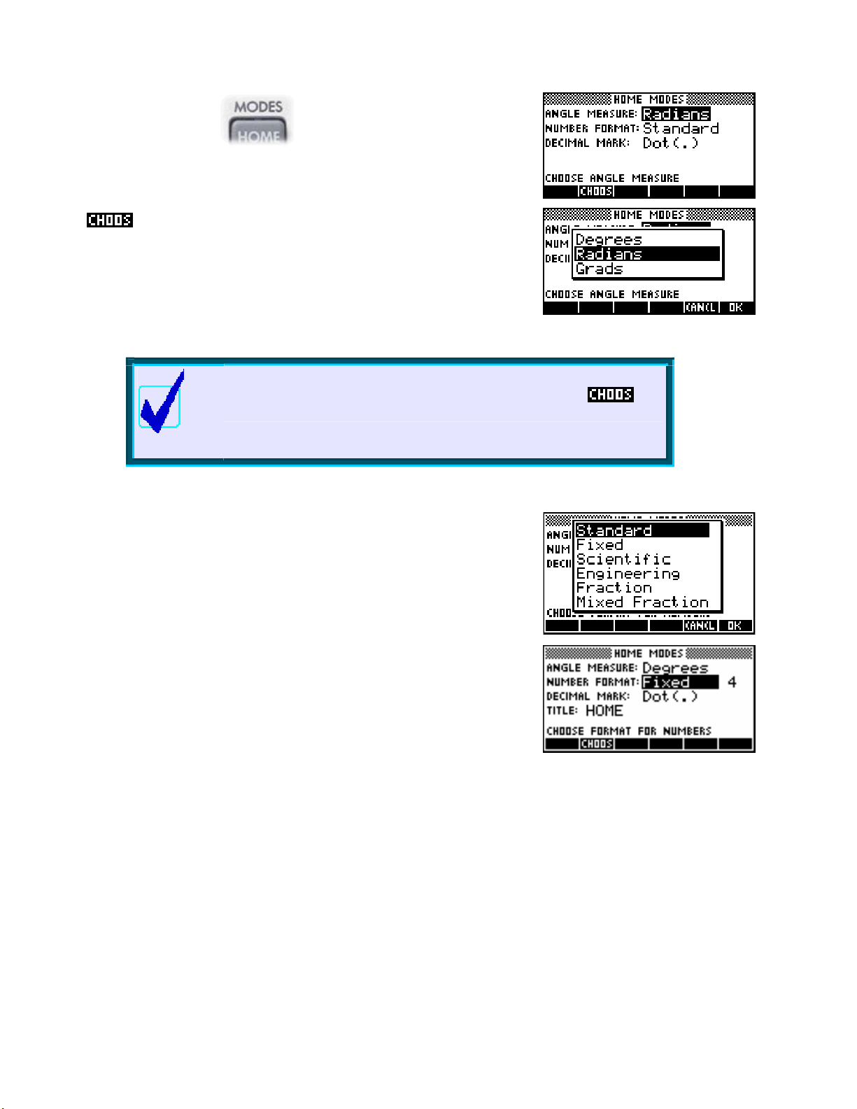
The MODES view

The

MODES view (see right) controls the numeric format used in

displaying numbers and angles in aplets. At the bottom of the screen you will see that one of the screen keys has been given the function

. Pressing this key pops up a menu of choices from which you can select the option which suits you. The default angle setting is radians.

Calculator Tip

If you don’t want to use the menu then, rather than pressing highlight the field and then press the ‘ ’ key repeatedly. This will cycle

through the choices without popping up a menu. This can be much faster if the menu has only a few choices.

Numeric formats

The choices for ‘

Number format’ are shown on the right. Standard is

probably the best choice in most cases, although it can be a little annoying to constantly have 12 significant figures displayed. In

Standard mode, very large and very small numbers are displayed in

scientific notation.

Fixed, Scientific and Engineering formats all require you to

The specify how many decimal places to display. The screenshot right shows

Fixed 4, which rounds everything off to 4 decimal places. Of course,

you can change the

A setting of

Scientific ensures that any results are displayed in scientific notation. Of course, the

4 to any other number you want.

calculator’s idea of scientific notation may not be the same as yours. Since the calculator has no way of displaying powers as superscripts, a result of

Engineering is very similar to Scientific, except that powers are displayed as multiples of 3 (ie. 10 ,10

3203 ×10

has to be displayed as 3.203E4. The alternative of ⋅

This is done to allow easy conversion in the metric system, which also works in multiples of 1000.

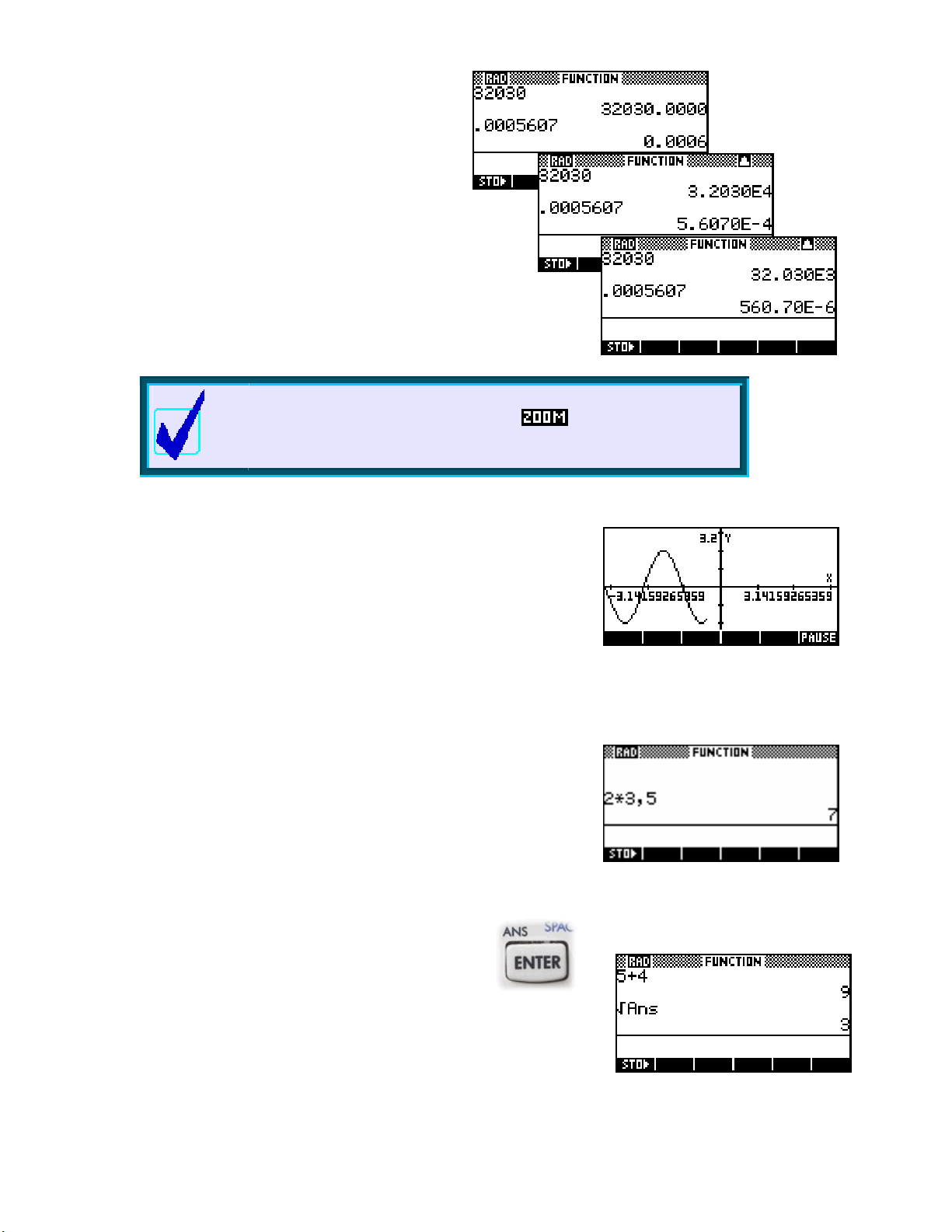
The screens right show the same two numbers displayed as in turn as;

Engineering 4.

Fixed 4, Scientific 4 and

Calculator Tip

If you have Labels turned on when you in (or out) on a graph or choose a Trig scale then you may end up with axes whose numeric labels are horrible decimals (see below right).

The setting of in more detail on page

The next alternative in the

Fraction can be quite deceptive to use and is discussed

33.

MODES view of Decimal Mark controls the character which is used as a decimal

point. In some countries a comma is used instead of a decimal point.

If you opt to use a comma rather than a full stop then any places where a comma would normally be used (such as in lists) will swap to using a full stop. Any functions which might normally have terms separated by a comma will use a full stop instead. For example, become

ROUND(3,456.2).

ROUND(3.456,2) will

Moving back to our tour of the keyboard, the next key is

ENTER key. This is used as an all purpose “I’ve

the finished - do your thing!” signal to the calculator. In situations where you woul

ators, press the

calcul

key. This can be used to retrieve the final value of the last

ANS

d normally press the ‘

ENTER key instead.

=’ key on most

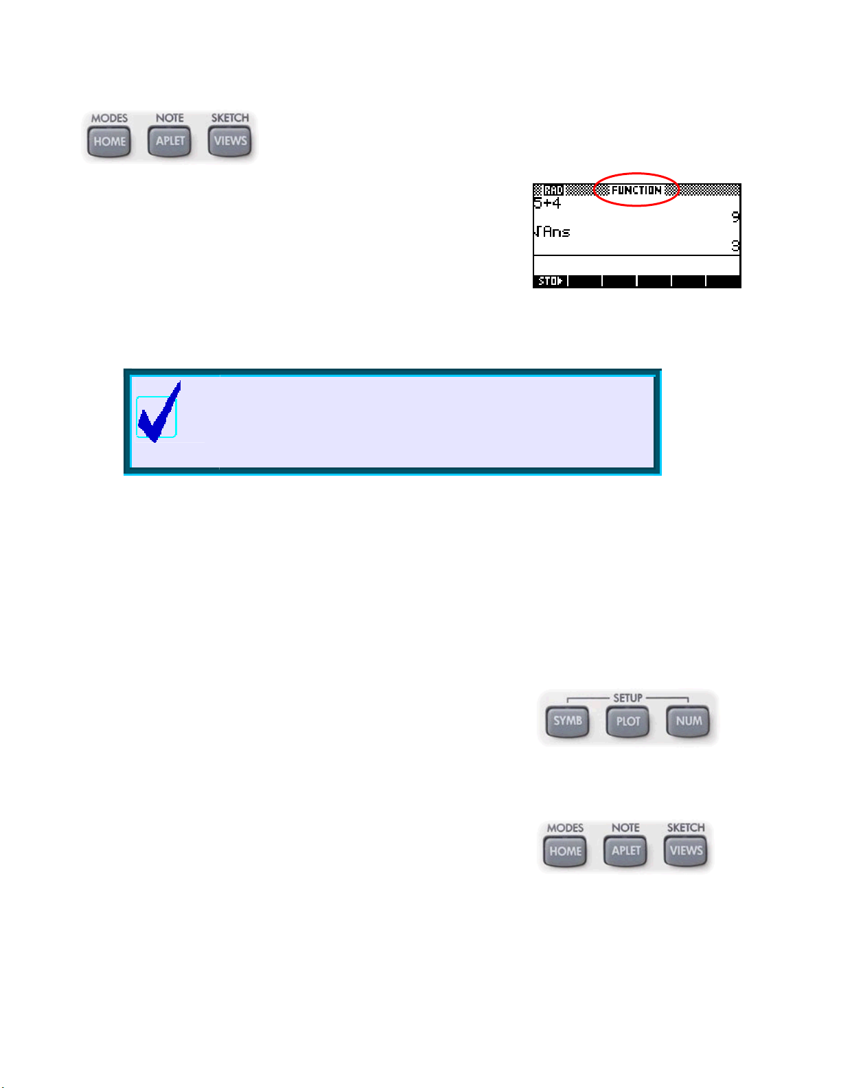
Above the

ENTER key is the

calculation done. An example is shown right.

The ANS key

−

If you are not confident about using brackets, then the ANS key can be quite useful.

372

For example, you could calculate the value of

2 5

by using

brackets…

…. or you could use the ANS key.

A better alternative to using the the

function. This is discussed on page 37.

ANS key is to use the History facility and

The negative key

Another important key is the

(-) key shown left. It is important to realize that the

hp 39gs and hp 40gs do not treat a negative as being the same as a subtract.

If you want to calculate the value of (say)

−−2(9) then you must use the (-) key

before the 2 and the 9 rather than the subtract key. If you press the subtract key twice, entering ‘subtract, subtract 9’ instead of ‘subtract (-) 9’ you will receive an error message of “Invalid syntax”, meaning it does not make mathematical sense to have two subtract signs rather than a subtract of a negative.

Similarly, if you press ‘subtract 2’ as the first keys in the above calculation then the calculator will display

Ans - 2. The reason for this is that a subtract cannot start an expression in mathematics, while a negative

sign can. Since the subtract can’t come first, the calculator decides that you must have intended to subtract from the previous answer. Hence the sudden appearance of an common error by new users is to enter a value into the

PLOT SETUP view using subtract instead of negative.

Ans. This occurs at other times too. A

This will usually have unexpected results.

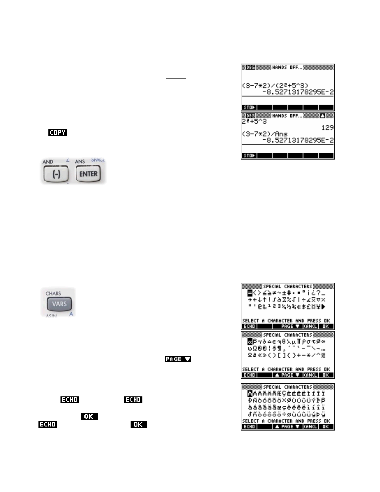
The CHARS key

The next important key is the

VARS). It accesses a view containing the characters

CHARS key (above

that are required occasionally but not often enough to bother putting on the keyboard.

Pressing the screen keys is set to be a ‘Page Down’ key

SHIFT CHARS will pop up the screens shown right. One of

, and will give

access to two more pages of characters as shown.

These special characters are obtained by pressing the screen key labeled

. You can press as many times as you need to in order to obtain multiple characters. When you have as many as you need, press the

is not required – just press

key. If you only require one character then

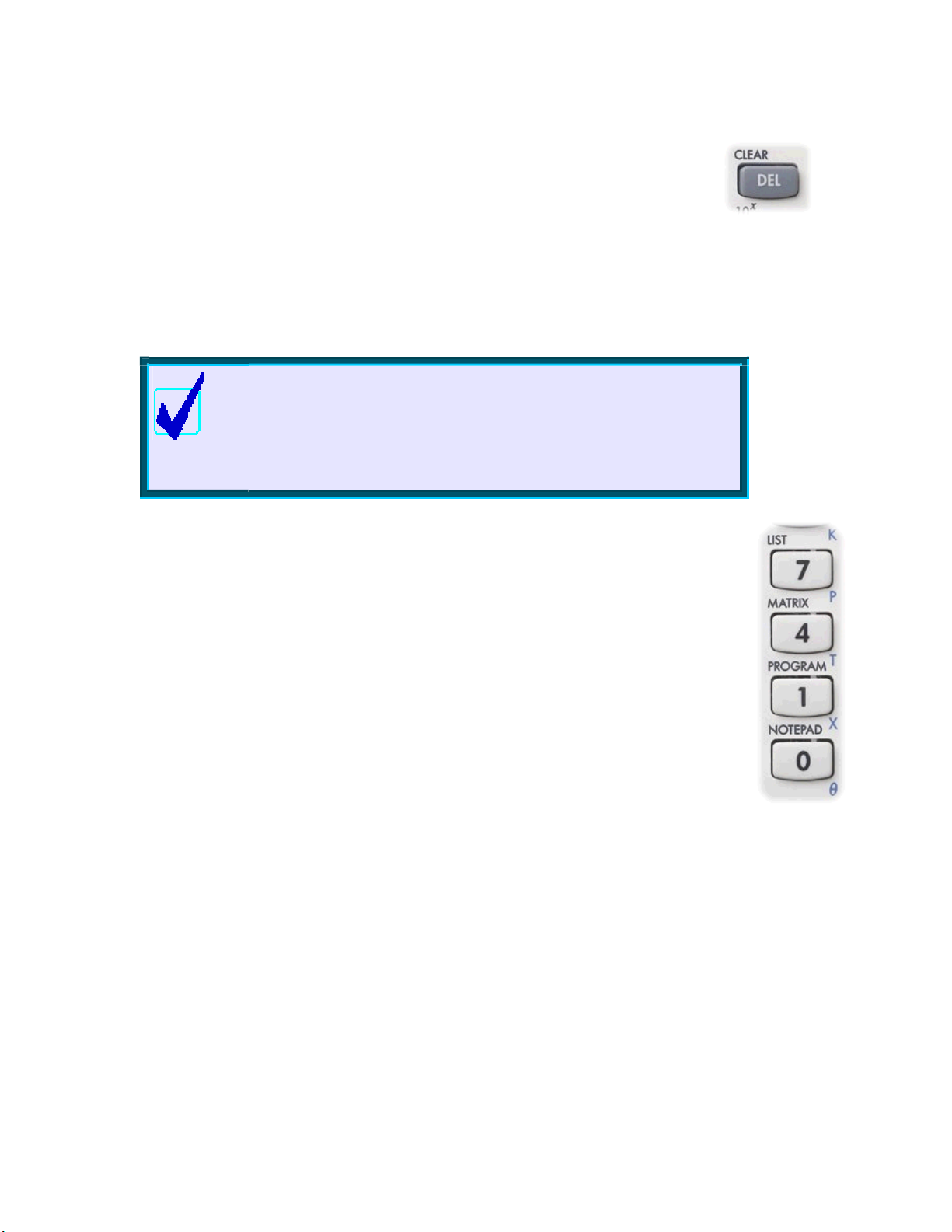
The DEL and CLEAR keys

Another important key is the

DEL key at the top right of the keyboard. This serves as a

backspace key when typing in formulas or calculations, erasing the last character typed. If you have used the left/right arrow keys to move around within a line of typing, then the

DEL key will delete the character at the cursor position.

CLEAR key above DEL can be thought of as a kind of ‘super delete’ key. For example, if pressing DEL

The would erase one function only in the

SYMB view then CLEAR will erase the whole set.

Calculator Tip

Another use for the DEL For example, if you move back into the screen and change to Degree mode, then pressi DEL lt of Radians. Pressing

CLEAR in the MODES view would restore factory settings to all the

ng the key will restore the defau

entries. This is particularly useful in the

key is to restore factory settings.

MODES

PLOT SETUP

view.

The remaining keys of chapters of their own.

LIST, MATRIX, MEMORY, NOTEPAD and PROGRAM have special

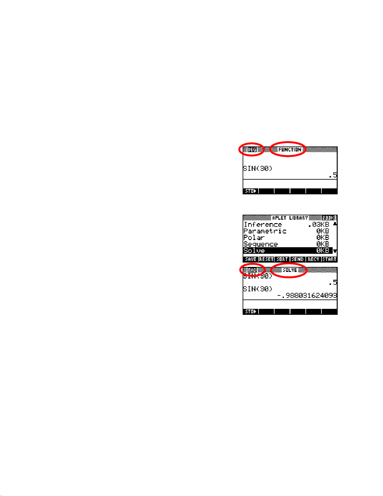
AAnngglleeaannddNNuummeerriiccsseettttiinnggs

It is critical to your efficient use of the hp 39gs and hp 40gs that you understand how the angle and numeric settings work. For those few who may be upgrading from the original hp 38g released in the mid ‘90s this is particularly important, since the behavior is significantly different.

On the hp 39gs and hp 40gs, when you set the angle measure or the numeric format in the applies both to the aplet and to the aplet (the one highlighted in the

HOME view. However, this setting applies only to the currently active

APLET view).

This means that if you change active aplet then these settings may change also, not only for the aplet but in the

HOME view too.

For example, suppose you have been performing trig calculations in the

HOME view with the Function aplet being currently active, and have set

the angle measure to

DEG.

If you were to now change to the Solve aplet in order to solve an equation then the settings would revert to those of the Solve aplet; probably be radians unless you had also changed those as well.

Radian measure is the default for all aplets and thus also for unless you change it. Performing exactly the same calculation in

HOME

would now give a different result, as shown right.

MODES view, it

Although this may seem to be a strange way of doing things, there is actually a very good reason for it. On the original first model, the hp 38g, the settings for the

HOME view were independent from those of the aplets

and it caused a number of users to have difficulties as you'll see on the next page.

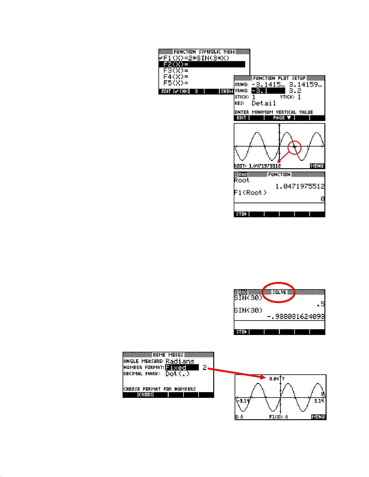
Suppose we define a trig function in the

Function aplet as shown.

The default setting for the Function aplet is radians, so if we set the axes to extend from -

to π, the graph would

look as shown right.

PLOT

In the

view shown, the first positive root has been

found (see page 57) as x=1.0471…

On the hp 39gs and hp 40g, if we now change to the retrieve the root and perform the calcul

ation shown right, we expect that

the answer should be zero, as indeed it is.

HOME

view,

However, this is only the case because the angle measures of problem was that on the original hp 38g the default setting for the Function aplet was radians, while

HOME and the Function aplet agree. The

HOME

had a default setting of degrees and its setting was independent of those of the aplet. This meant that a calculation such as the one above would give incorrect results, and caused considerable confusion to some students. It even resulted in users returning their hp 38g to dealers as being ‘faulty’! Hence the change, which was first made in the hp 39g and hp 40g.

The only drawback of synchronizing the settings of the

HOME and aplet

is that you might change aplets and forget that it may also change the

HOME view settings. For this reason, the name of the active aplet is

shown at the top of the

HOME view as a reminder.

On the hp 39gs and hp 40gs you can see that if we turn

Labels on and then PLOT,

the numeric mode also affects the axis labels.

The default behavior in the

PLOT view is to not display axis labels due

to the way that they often interfere with the clear display of the graph.

Settings made in the

SHOW command, covered on page 38.

MODES view also apply to the appearance of equations and results displayed using the

Calculator Tip

Under the system used on the hp 39gs and hp 40gs, if you want to work in degrees then you will need to choose that setting in the MODES view and possibly set it again if you change to another aplet. Some people choose to go through and change the setting on all the aplets at once so that they don’t have to remember that it might change. However, if you an aplet or reset the calculator then the default setting will return.

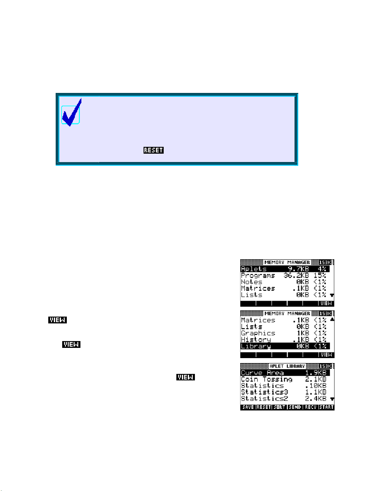
MMeemmoorryyMMaannaaggeemmeennt

One of the major complaints about the original hp 38g was its memory - mainly the lack of it at only 23Kb, but also the inability to easily control or manage it. This problem has been addressed on the hp 39gs and hp 40gs in two ways. Both have a very ample amount, just short of 200Kb, and there are very few users who will come close to filling this. Depending on size, there is enough room for at least 40 aplets, 40 pages of notes, or nearly 10,000 data points although not, of course, all at once.

The MEMORY MANAGER view

In addition to all this memory, the hp 39gs and hp 40gs supply an easy way to control it through the

MEMORY key you will see the view shown right. Scrolling through it

the will show you exactly how the available memory is currently being used. The remaining memory, in Kb, is shown at the top right of the screen. This view gives an overview of the memory. For detailed management the

Pressing you can delete entries no longer needed.

key is provided.

on any entry will take you a relevent screen in which

MEMORY MANAGER view. If you press

For example, with the highlight on Aplets, pressing

APLET view (right), where you can choose to delete or reset any

to the aplets no longer required.

will take you

As you can see in the screen snapshot on the previous page, my calculator has a number of extra aplets. Two of them, Statistics2 and Statistics3 are simply copies of the normal Statistics aplet containing data that I did not want to lose. The top two aplets Curve Area and Coin Tossing are teaching aplets that I have downloaded from the internet.

Downloaded aplets & memory

If you use teaching aplets that you download from the internet via the Connectivity Kit, or which are supplied to you by your teacher via the infra-red link on an hp 39gs or the cable on an hp 40gs, then you need to bear in mind that most of them have ‘helper’ programs that aid them in performing their tasks.

In the screens shown right you can see some of the programs which are attached to the two aplets mentioned above. The convention which most programmers follow is to name these ‘helper’ programs in a way that associates them clearly with the parent aplet. The memory associated with these programs is not included in that shown for the aplet in the

APLET view but will not usually be a very large amount, as you can see

in the examples shown.

Calculator Tip

The reason for this naming convention for ‘helper’ programs is that when you delete the parent aplet in the

APLET view the ‘helper’

programs are NOT automatically deleted with it because they may be shared by other aplets.

You must change to the

Program Catalog

view and delete them manually after you have finished with the teaching aplet and deleted it in the If you don’t do this

APLET view.

then they will continue to take up memory on the calculator. the hp 39gs and hp 40gs this is not infinite and too many left over programs will eventually cause problems.

As mentioned on the earlier, pressing

MANAGER

screen takes you to a relevent view showing greater detail.

in the MEMORY

For example, the Matrices entry right shows 0.1 Kb in use. Pressing

will take you to the MATRIX CATALOG view which shows exactly where the memory is being used and allows you to delete any or all of the matrices. Alternatively, you can enter the view in the normal way by pressing

The History entry will take you to the

SHIFT CLEAR will clear the History.

SHIFT 4.

HOME view, where pressing

Even on

The GRAPHICS MANAGER

There are two views, shown right, for which the only access is via the

MEMORY MANAGER screen. The first of these, the GRAPHICS

MANAGER

, shows some memory in use on my calculator due to the screen captures I am performing to show you these views. Yours will probably be empty. If you have loaded an aplet from the internet then it may have used a GROB (Graphics Object) to store an image as part of its working.

The LIBRARY MANAGER

The second view is the

LIBRARY MANAGER, and this will almost

certainly be empty unless you have games loaded. Generally, the only aplets which use libraries are those such as games which are written by expert programmers in machine code in order to make them run as fast as possible. These games, available on the internet, are listed in the

APLET view along with the normal aplets and when you delete them the associated library is automatically

deleted with them, unlike the case of the ‘helper’ programs.

Calculator Tip

Because of the amount of memory available on the hp 39gs & hp 40gs, the Memory View is not one that you will normally need to worry about unless you store a tru y amazing number of Notes. It

is probably of more interest to programmers.

As discussed later, most games currently available for the hp 39gs and hp 40gs were originally written for the hp 39g. This can cause problems in two respects:

• l

The hp 39g was a much slower calcu ator and the games may simply run too fast to be playable.

•

Some games were written using programming commands specifically aimed at the hp 39g chip. When these commands execute on an hp 39gs or hp 40gs they may cause the

calcu ator to lock up and/or lose user memory. They should not, however, cause permanent damage.

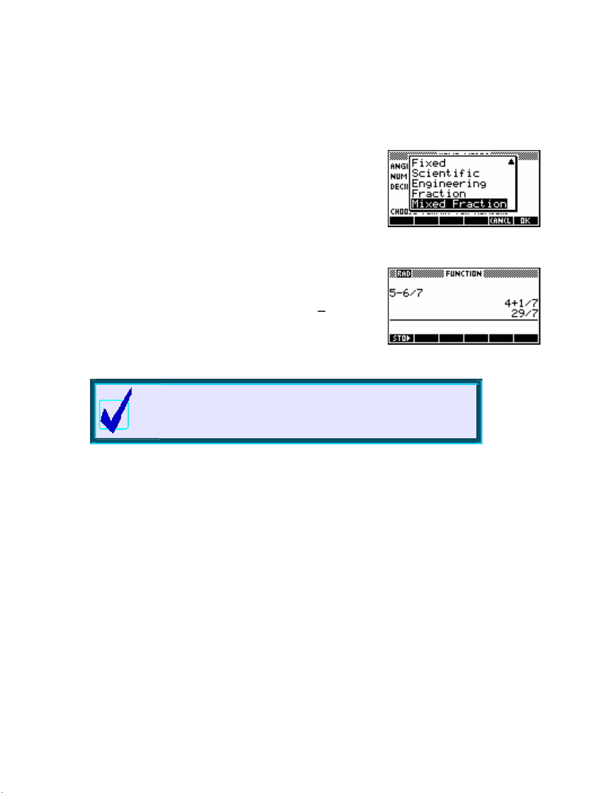
FFrraaccttiioonnssoonntthheehhpp3399ggssaannddhhpp4400ggs

Earlier we examined the use of the

Number Format. We discussed the use of the settings Fixed, Scientific and Engineering, but left the setting of Fraction for later.

The reason for this is that the Begin by selecting

Fraction in the MODES view, leaving the

accompanying number as the default value of

Most calculators have a fraction key, often labeled

MODES view, and the meaning of

Fraction setting can be a little deceptive.

, that allows you to input, for example,

12¬¬3 or something similar. What these calculators usually won’t do is allow you to mix fractions and

decimals. A calculation such as

to convert the

37 into a fraction. The reason for this is that while some decimals like 0.25 are easy to⋅

13 +⋅

3 7

will usually give a decimal result: most calculators will not attempt

convert to a fraction, others, such as recurring ones, are not so easy. Most calculators opt for the easy option of switching to a decimal answer in any mixture of fractions and decimals. When making the hp 39gs and hp 40gs HP took a very different approach. Once you select

Fraction mode, all numbers become fractions -

including any decimals.

The first point to remember is that there is no provision for inputting

mixed fractions such as

. Fractions are entered using the divide key

and, while the calculator is quite happy with improper fractions such as

5/3, it correctly interprets 1/2/3 as ½ divided by 3 and gives a result of 1/6 . The solution to this is simply to enter mixed fractions as (1+2/3).

Calculator Tip

You need to be careful with brackets or else “order of operations” problems may occur, such as

1+(2/3*1/5) rather than as it should be: (1+2/3)*1/5.

When in doubt, use brackets for mixed fractions.

Some examples are… (using a setting of

14 17

35 15

1 1 1

3 − 4 = −1

3 2 6

Fraction 4 or higher)

being interpreted as

The second point to remember involves the method the hp 39gs and hp 40gs use when converting decimals to fractions, which is basically to generate (internally and unseen by you) a series of continued fractions which are approximations to the decimal entered. The final fractional approximation chosen for display is the first one found which is ‘sufficiently close’ to the decimal. Look up ‘continued fractions’ on the web or in a textbook if you don’t know what these are.

The trap lies in what constitutes ‘sufficiently close’, and this is determined by the ‘

4’ in Fraction 4. Very

roughly explained, the calculator will use the first fraction it finds in its process of approximation which matches the decimal to that number of significant digits.

For example, a setting in the

Fraction 1

MODES view of…

changes 0.234 to

which is actually 0.2307692…

(matching to at least 1 significant figures.)

Fraction 2

changes 0.234 to

which is actually 0.2333333…

(matching to at least 2 significant figures.)

Fraction 3

changes 0.234 to

11 47

which is actually 0.2340425…

(matching to at least 3 significant figures.)

Fraction 4

changes 0.234 to

117

500

234

⎛

⎜ ⎝

1000

⎞ ⎟

⎠

which is exactly 0.234

(thus finally matching to the required 4 significant figures.)

Essentially, the value of

4 in Fraction 4 affects the degree of precision used in converting the decimal to a

fraction. As was said earlier, the calculator will use the first fraction it finds in its process of approximation which matches the decimal to that number of significant digits.

The

Fraction setting is thus far more powerful than most calculators but

can require that you understand what is happening. It should also be clear now why a special fraction button was not provided: the ‘fractions’ are never actually stored or manipulated as fractions at all!

Pitfalls in Fraction mode

As you can see above right, a setting of

0.666, while adding one more 6 (to take the decimal beyond 4 d.p.) will give the desired result of

Fraction 4 produces a strange (but actually correct) result for

2/3. In

other words, so long as you understand the approach taken by the hp 39gs and hp 40gs it is capable of producing results which are closer to what was probably intended by the user in entering 0.66666.

You may have noticed that all the results so far have been improper fractions. For example the first calculation shown right gives the answer

. The fraction setting of Mixed Fraction is

as 22/15 rather than

essentially the same but answers are given as mixed fractions instead of improper fractions, as shown.

If you want to use the

Fraction setting to convert decimals to fractions, here are some tips…

• if converting a recurring decimal to a fraction, then make sure

you include at least one more digit in the decimal than the setting of

Fraction in MODES. As you can see right, failing to

include enough decimal places does not produce the desired result.

• if you are converting an exact decimal to a fraction, then set a

Fraction n value of at least one more than the number of

decimal places in the value entered. Both examples in the third screen shot to the right were done at

Not understanding the significance of the setting of produce some unfortunate effects. For example, at Fraction

123.456 becomes 123, with the 0.456 dropped entirely.

Fraction 6.

Fraction can

2, the value

An example of this is shown right. If you use a setting of only

Fraction 2

to perform the calculation shown, you will find to your amazement that

1/3 + 4/5 = 8/7 , whereas using Fraction 6 gives the correct answer.

The reason for this ‘error’ is that the

1.133333…. This was converted back to a fraction using Fraction 2 to give 8/7 (1.1428..).

1/3 and 4/5 were converted to decimals and added to give

This may seem odd but it does match sufficiently closely in

Fraction 2 to be accepted.

Generally it is not a good idea to go below the default setting of

Fraction 4. In fact, a Fraction 6 setting tends to be more reliable.

A new feature of the hp 39gs and hp 40gs is the setting of

Fraction

in the MODES view.

Mixed

The results of this new setting can be seen in the image to the right.

Using the setting of

Mixed Fraction the result is 4+1/7 (

) whereas

the answer of

29/7 is obtained using the old Fraction setting.

Calculator Tip

If you scroll back through the History and re-use a result such as the

4+1/7

shown above then don’t forget to put brackets around it to ensure

that no ‘order of operations’ errors occur.

TThhe

HHOOMME

HOME page maintains a record of all your calculations called the History. You can re-use any of the

The calculations or their results in subsequent calculations.

Try this for yourself now. Type in at least four calculations of any kind, pressing the the calculation.

You will now be looking at a screen similar to the one on the right (except probably with different calculations).

If you now press the up arrow key, a highlighted bar moves up the screen. When you reach the top of the screen the previous calculations will scroll into view. Pressing top in one movement.

COPYing calculations

You may have noticed that as soon as the highlight appeared so did two labels at the bottom of the screen. If you now press the screen key under

the edit line. This is shown in the screen shot on the right.

HHiissttoorry

ENTER key after each one to tell the calculator to perform

you will find that the highlighted calculation will be copied on

SHIFT up-arrow takes the highlight to the

At this point you can use the left and right arrows and the of the characters and/or adding to it.

For example, in the screenshot right, the calculation of has been edited to

Clearing the History

Pressing enter will now cause this new calculation to be performed.

3*COS(35).

Calculator Tip

Pressing ON during editing will erase the whole line. Pressing SHIFT CLEAR erases the whole history. This is worth doing regularly, since the history uses memory that may be needed for other things, even with the immense amount of user memory the hp 39gs & hp 40gs have. You can calculations and results from any number of different lines in building your new expression.

DEL key to edit the calculation by removing some

3*2*COS(35)

SHOWing results

Next to the

key you will see another screen key labeled . This key will display an expression the way you would write it on the page rather than in the somewhat difficult to read style that is forced on the calculator when it must show the whole expression on one line. This works anywhere the appears, not just in

HOME. Some examples…

label

SSttoorriinnggaannddRReettrriieevviinnggMMeemmoorriiees

−

Each of the alphabetic characters shown in orange below the keys can function as a memory. Some examples of this are shown in the third of the four examples above where the values of stored into

A, B and C prior to the use of the quadratic formula. All of this storing of values is done with the

1, -3 and -4 are

key, which is one of the screen keys listed at the bottom of the HOME view. There are ways of

obtaining even more memories than these 26 alphabetic ones, such as storing values into a list (see page

215), but 26 is enough for most purposes.

Once stored into memory, values can be used in calculations by typing the letter in place of the value. Typing a letter and pressing

ENTER will

display memory’s contents. See right.

There is an advantage to storing results in memories, particularly if they are long decimals, or if you’re going to be re-using the result a number of times.

4(3)

As an example, we will perform the calculation of

−

23 5

⋅−

We will do this in two stages, calculating the top and bottom of the fraction and storing the results in memories.

Firstly the top of the fraction, storing the result in memory bottom, storing in

As another example, suppose we were evaluating value

x =−3 . We can store -3 into the memory X and then use that

B, and then finally the result…

3xx2+ 7 for the

A, then the

symbol in the calculation as shown right. The advantage of this is that if we now wanted to evaluate that expression for other values then we need only store a different value into X and then

the expression for re-evaluation. Clearly, if the expression is complex, this can be very helpful.

Calculator Tip

1. The memory X is the exception to the above information. It is used to store the current cursor position in the PLOT view so that you can access it in other places. Values stored in X will be overwritten the next time you use the PLOT view.

2. A common error is to forget to put brackets around negatives when evaluating expressions with powers. For example, evaluating

as -32 – 1 rather than as (-3)2 – 1. This can be avoided by

1x −

storing the value into memory X and evaluating X2 -1. This is particularly useful in very complex expressions. Any memory can be used in this way, not just X.

RReeffeerrrriinnggttooootthheerraapplleettssffrroommtthhe

HHOOMME

vviieeww.

Once functions or sequences have been defined in other aplets, they can be referenced in the

e.g. 1 Suppose we use the Function aplet to define

F1(X)=X²-2 and F2(X)=e

These functions now become accessible not only from within the

as shown right.

HOME

view but also within any other aplet also. This is shown by the screen shots below.

The results shown will, of course, depend on your settings in the

MODES

view.

The reason for the

QUOTE(X-2) rather than just X-2, is that using X-2

would tell the calculator to use the value currently stored in memory X,

QUOTE(X-2) tells it to use the symbol. The QUOTE function is

while available through the

MATH menu under Symbolic (see page 181).

HOME view.

Note: This type of work is actually far more easily done in the Function aplet, where better job. See page

QUOTE is not needed and the key does a

64.

e.g. 2 Suppose we use the Sequence aplet to define a sequence

with

In the

= 3, 12 = and Tn = 2 T

HOME view, the sequence values can be referred to as easily as

n−1

+ T

n− 2

the function values in the previous example.

You could also define a function refer to this function in the

F1(X)=1000.

F1(X) in the Function aplet and then

Solve aplet to find, for example, where

AAbbrriieeffiinnttrroodduuccttiioonnttootthheeMMAATTHHMMeennu

MATH menu holds all the functions that are not used often enough to be worth a key of their own. There

The

is a very large supply of functions available, many of them extremely powerful, listed in their own chapter beginning

on page 165.

When you press the

MATH key you will see the pop up screen shown

right. The left hand menu is a list of topics. Scroll through the topics until you find the one you want, then use the right arrow key to move into the list of functions for that topic.

For example:

The function

ROUND will round off to a specified number of decimal

places.

E.g. round off 145.25667 to 3 decimal places.

Press the

Press the ‘ beginning with ‘R’, then move down one more function to Press

MATH key & right arrow ( ) into the Real group of functions.

R’ key (the 9 key) to move to the first of the functions

ROUND.

ENTER.

Now finish off the command and press

ENTER again to see the result.

For more information on the Math Menu, see page

165.

RReesseettttiinnggtthheeccaallccuullaattoor

It is probably inevitable as the line between calculators and computers becomes blurred that calculators will inherit one of the more frustrating characteristics of computers: they crash! The hp 39gs and hp 40gs can sometimes do this due to the very complex and flexible operating system they use. If you find that the calculator is beginning to behave strangely, or is locking up then there are a number of ways to deal with this.

Calculator Tip

If you are a user of external aplets then you may occasionally find that an aplet that has been working perfectly will unexpectedly stop working with the message “Invalid syntax. Edit program?”. There is almost certainly nothing wrong. Press , try a soft reboot as below, then run the aplet again.

Soft reboot (Keyboard)

Pressing that your third screen key from the left. The calculator will very briefly display a boot screen and then redisplay the

HOME view, with the Function aplet as the active one.

If you find that the calculator locks up so completely that the keyboard will not respond then a method of reset is provided below which is independent of the keyboard. This shouldn’t happen but it is important to know how to deal with it in case it happened during a test or an exam.

Thi s method is provided in case the calculator is locked up to the point that the keyboard no longer responds.

On the back of the calculator is a small hole. Poke a paper clip or a pin into this hole and press gently switch inside. This briefly interrupts the power supply and, to the calculator, is exactly equivalent to a soft reboot as outlined in the previous section. Normally it should not only unlock the calculator but retain your data intact. However, it must be pointed out that a problem so severe that it has locked up the keyboard may be so bad that it has corrupted the memory anyway. If so then you may find that you see the “Memory Clear” message when it reboots. If you find that it keeps locking up repeatedly then you should perform a hard reboot as described in the next section. If you have important data on the calculator then you might try to save it to a PC before doing this since a hard reboot will wipe all user memory.

ON+SK3 will perform a soft reboot. It is perfectly safe and will not cause any memory loss except

HOME History will be cleared. Hold down the ON key and, while still holding it down, press the

Soft reboot (Hardware)

on the

Hard reboot (with loss of memory)

To completely reset the calculator’s memory back to factory settings press 1”) When doing this, don’t press them all at once; hold down the

ON key and, while still holding it down,

press the first and then the last screen keys. Release them in the opposite order. Don't release together - release

SK6, then SK1, then ON. This is deliberately made complex so that it won’t happen by

ON+SK1+SK6. (SK1=”screen key

SK1 and SK6

accident!

This type of reset will always cause complete loss of data. If you find that the screen fills with garbage, or if the calculator’s in-built diagnostic routine starts to run, then it is just that you have not released them in the right order. Simply try again.

Calculator Tip

If your calculator is really thoroughly locked up or won’t turn on then try the procedures listed below this tip.

My past experience with these calculators is that they do tend to lock up occasionally, particularly if you load aplets and programs from the web.

I usually suggest to my students that they regularly save their work to a PC and perform a hard reboot about once a month, reloading the saved work onto the calcu

3. ON+SK4

Pressing by mistake will

lator afterwards.

result in the screen shown right. This is a special diagnostic mode that can be used by engineers to test the calculator’s components. There is nothing wrong with experimenting with it but it is of no use to the average user. To exit, simply reboot normally by pressing

ON+SK3

Locked Calculator? Won't turn on? Turns on briefly and then immediately off?

Try the following:

• Try a soft reboot using ON+SK3.

• Try a paperclip in the hole in the back (gently).

•

Is it possible that the screen is blank because the contrast is turned to extremely light? Try

ON and to make the screen darker. (Hold down ON and press repeatedly.)

ON and to lighten the screen.

Use

• Change the batteries for new ones. Try this more than once because sometimes batteries are dead

right off the shelf if they've been in the shop too long. Try replacing the backup battery too. Make SURE you’ve put the batteries in right way around. Putting them in reversed may seriously damage the calculator.

• Take the batteries out, including the round backup battery. Press and hold the ON button for 2

minutes to remove any possible remaining power from the internal capacitors. Leave the calculator overnight and re-insert fresh batteries.

• If this happened when running a game or aplet that you've downloaded from the internet then

consider that this may be the source of the problem. Backup anything that you want to keep to the PC and do a full reboot to restore factory settings.

• Try a full reboot using ON+SK1+SK6.

Some less likely options:

• Did the paperclip feel funny when you inserted it? There should be a very subtle sensation of

'pressing a button' as the paperclip shorts out the batteries momentarily. Could you have accidentally bent the shorting contact last time you used a paperclip so that it is permanently shorting out?

• Check the battery compartment. Are any of the metal contacts broken or out of place? Are the

batteries firmly in contact with all of them? Is anything out of place? Do any of the batteries or the metal contacts show corrosion? If so, clean them carefully, being careful not to get moisture inside the calculator.

• Have you recently dropped the calculator or spilled liquid on it? If so, this is not good. It is probably

permanently dead. Did you need a very expensive paperweight?

• Check the USB and Serial ports at the top of the calculator. Do they have anything wedged in them

courtesy of a young child perhaps?

SSuummmmaarry

• The up/down arrow key moves the history highlight through the record of previous calculations.

When the highlight is visible, the using the left/right arrow keys and the

key can be used to retrieve any earlier results for editing

DEL key.

• Care must be taken to ensure the your idea of order of operations agrees with the calculator’s.

For example, (-5)

must be entered as (-5) 2 rather than as -52, and 54must be entered as

√(5+4) rather than √5 + 4.

• The ANS key can be used to retrieve the results of the calculation immediately preceding the one

you’re working on. E.g.

√(5+Ans)

• The DEL key can be used to erase single characters in the editing line or single lines in the HOME

history. The

SHIFT CLEAR key will delete the entire history. Regular clearing will ensure that

memory is not gradually eroded.

• The key displays a calculation as you would see it written and is available in many views.

• The MODES view can be used to set the format in which numbers are displayed on the HOME page,

and to choose the angle measure which is to be used.

• Make sure you understand Fraction mode before using it.

• Remember that the angle and numeric mode settings may change if you change aplets in the APLET

view.

• Numbers are stored in memory using the key labeled . The stored values can then be used by

simply putting the letter in the expression in place of the number.

• You can easily reboot the calculator if it locks up, generally without loss of memory. Make sure you

know how to do this in case it happens during a test or an examination.

• Regularly saving your information to a PC will ensure that you don’t lose anything important.

Additionally, it is a good idea to completely reset the calculator occasionally so that any instability in the operating system has no chance to grow.

• Many extra functions are available via the MATH menu. For more information on the complete set of

mathematical functions available in the menu” on page

165.

HOME view (and anywhere else) see the chapter “The MATH

The Function aplet is probably the one that you will use most of all. It allows you to:

Choose the aplet

The first step for any aplet is to choose it in the Press the the right. Use the arrow keys to move the highlight up or down until the Function aplet is selected. Now, looking at the list of context sensitive functions at the bottom of the screen, you should see labels of and

HHE

UUNNCCTTIIOON

• graph equations

• find intercepts

• find turning points (maxima/minima)

• find areas under curves

• find areas between curves

• find gradients

• find derivatives algebraically

• find simple integrals algebraically

• evaluate functions at particular values

• graph and evaluate algebraically expressions such as f(g(x)) or f(x+2)

APLET key and you will see something similar to the screen on

PPLLEET

APLET LIBRARY.

Press the key under press the functions that you may have put in there while playing around, and so to make sure that what you see will be the same as the screen snapshots.

key. The reason for doing this is to clear out any

first. You’ll see the message shown right -

The SYMB view

Now press the so that it appears like the one on the right. This is the

key. When you do, your screen should change

SYMB view.

Notice that the screen title is supplied so that you will know where you are (if you didn’t already).

Calculator Tip

Pressing d have had the same effect.

ENTER rather than woul

Whenever there is an obvious choice pressing produce the desired effect.

The

button

ENTER will usually

Whenever you enter an aplet, one of the keys which often changes its function is the key labeled label suggests, it supplies an produce a graph of the quadratic we dealt with in the earlier section on the

Using the up/down arrows, move the cursor (if necessary) to the line labeled

X, or a T, or a θ, depending on which aplet you are in. Let's use that key to

HOME view.

F1(X) = .

XTθ. As its

Type in:

This will produce the screen shown on the right. Notice the check/tick mark next to the

F1(X) that appeared when you pressed ENTER. This

signifies that this function is to be graphed, so that if you had five functions entered but only wanted 1 and 3 graphed, you could simply ensure that only

F1(X) and F3(X) were checked.

ing your function

The key that turns the check on or off is a screen key - the one labeled with the

. In computer terminology it is a ‘toggle’ key - when the check is off it turns it on and when on it turns it off. In some countries a check mark is called a ‘tick’ but the idea is the same.

Try turning the check on and off for function

F1(X). Remember, the highlight has to be on the function before

the check can be changed. Make sure it’s checked when you have finished.

The NUM view

If you now press the

NUM key, you will see the screen on the right. It

shows the calculated function values for increasing in steps of

0.1

F1(X), starting at zero and

Make sure the highlight is in the You will find that the numbers will now start at four via the

key, which can be convenient at times, particularly for trig functions. The simplest way to set

the start value and increment is in the

X column as shown on the previous page, and then press 4 and ENTER.

instead of zero. It is also possible to change the step size

NUM SETUP view. This is covered in detail on page 70.

The PLOT view

Now press the

PLOT key. The graph you’ll see will not be a terribly

useful one (see right) because the axes will not be set up correctly. We’ll look next at how to do this.

One of the easiest ways to set up the axes properly for a function whose shape is not known in advance is to let the calculator suggest a suitable scale using the Auto Scale option in the

VIEWS menu covered on the next

page. However, its suggested scales are not always very helpful. There are a number of ways of working out a ‘nice’ scale. See page 78 for a discussion of this. Another method is to use the

NUM view to investigate the

range of values that will be required for the function.

More complete information on the

VIEWS menu can be found on page 85.

AAuuttooSSccaalle

Auto Scale attempts to fit the best possible vertical scale to the horizontal scale you have chosen. It is not always successful but will often give you a good starting point from which to refine the scale. In the example which follows it is assumed that you have plotted the graph as shown on the previous page.

PLOT view, press the VIEWS key. Use the arrow keys to scroll

In the down to Auto Scale and press

ENTER. The calculator will adjust the y

axis in an attempt to fit as much of the graph on to the screen as possible.

Some points to bear in mind;

• the y axis is scaled only on the first function which has a .

• the y axis is scaled for the current x axis (domain) you have chosen in PLOT SETUP. If you’ve not

chosen the domain wisely then your result may not be good.

• it doesn’t choose ‘nice’ scales for the y axis such as we would choose (going up in 0.2’s or 5’s or

10’s etc.) so you will generally need to tidy up its choice a little.

If you look at the y axis of the graph you’ve just produced, you’ll see that the axis tick marks are so close together that it looks like a solid line. To tidy this up you must change to the above the

SETUP’. The SETUP view for each of these keys is obtained via the

‘

SHIFT key.

PLOT, SYMB and NUM keys you will see the word

PLOT SETUP view. If you look

The values produced by the Auto Scale are shown below, along with a better set that produces a clearer

PLOT view. Note particularly the YTick setting that removes the ‘thick’ effect on the y axis.

See “The Expert” chapter beginning on page 62 for more information on how to find good choices for axes. The Auto Scale function is

also covered on page 89.

TThheePPLLOOTTSSEETTUUPPvviieew

In the information that follows it will be assumed that you have performed the tasks on the previous page.

If you press

SHIFT then PLOT you will see something like the view on

the right.

The highlight should be on the first value of XRng. Enter the value -4.

Calculator Tip

Don’t use the subtract key to enter a negative. You MUST use the negative key labeled (-). Similarly, don’t use a (-) when you mean a subtract. For example, 2 (-) X will produce -2*X not 2 – X.

Type in 4 for the other values. When you’ve done this use the arrow keys move to

XRng value, then -20 and 20 for the YRng

Ytick and

change it to 5.

Detail vs. Faster

At the bottom of the screen you will see

Res (short for ‘Resolution’). If you highlight it and press the

key you will see that you have a choice of ‘Faster’ or ‘More Detail’. ‘More Detail’ should be selected. If you choose Faster then every second dot is plotted instead of every dot. This is quicker but may make some graphs appear less smooth, particularly graphs with steep gradients.

There are two pages to this view (see the

key at the bottom of the screen). The first page is used to set axes, the second to control certain features of them.

If you press the

key you will now be looking at the screen shown above right. Using the arrow keys to move the highlight, make sure that your checks/ticks match the ones in my snapshot. Now press

PLOT again.

Let's have a look at the meaning of the CHKs (check marks or ticks) on the second page of

PLOT SETUP

above right. Although they are not used often they can be quite useful and I recommend highly that you at least consider using the Simult setting.

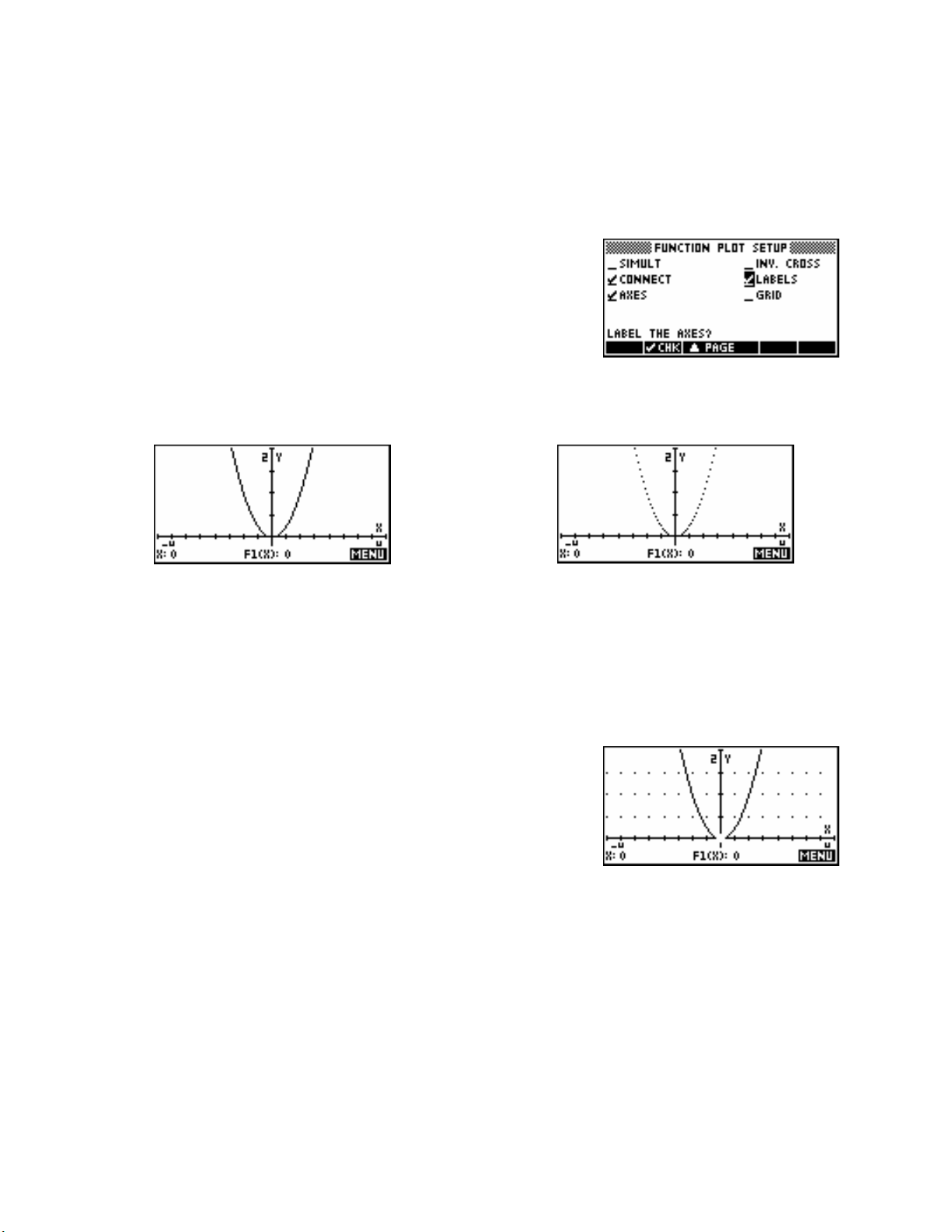
Simultaneous

The first option

Simult controls whether each graph is drawn separately (one after the other) or whether they

are all drawn at the same time, sweeping from left to right on the screen.

My preference is to turn this off. I find that if there are more than two functions defined then drawing them all at the same time can be confusing. Turning off

Simult means that they are drawn one after the

other, in the order that they are defined. This is obviously a bit slower but makes it easier to understand.

Connect

The second option

Connect controls whether the separate dots that make up a graph are connected with

lines or left as dots. This is very seldom of use.

vs…

Axes

The third option

Axes controls whether axes are drawn. The fourth Inv. Cross controls the appearance of

the cursor that is moved by the arrow keys. It is best if you try this one yourself to see the effect.

Labels

The fifth option

Labels controls whether labels (‘X’, ‘Y’) and a scale are put on the axes. The only time this

causes problems is if the scale is an odd one, causing the labels to have too many decimal places. If desired this effect can be offset by setting fixed decimal places in the

MODES view.

Grid

The sixth and last option

Grid causes a grid of dots to be drawn on the

screen (see right). The density of the grid is controlled by the values of

Xtick and Ytick. This can be quite useful.

TThheeddeeffaauullttaaxxiisssseettttiinnggs

The default scale is displayed in the may seem a strange choice for axes but it reflects the physical properties of the LCD screen, which is 131 pixels wide by 63 pixels tall. A ‘pixel’ is a ‘picture element’ and means a dot on the screen.

The default scale means that each dot represents a ‘jump’ in the scale of

0.1 when tracing graphs. The y value is determined by the graph, of course, and has nothing to do with your choice of scale. Once the scale changes, the size of the jumps from dot to dot are often not a useful size. See page

TThhe

The MENU toggle

If you look at the screen key list at the bottom of the screen you will see only a single entry, labeled

Press the key under it and your screen will change to look like the middle one of the three right.

62 for information on choosing ‘nice’ scales.

BBaar

PLOT SETUP view shown right. It

Press it again and the screen will clear completely. Once more and you are back to the original appearance. Try pressing it a few times to get the feel for its behavior. This is what is known as a ‘toggle’ switch. The of the display modes shown above and right. The first (default) mode is (X,Y) mode, where the coordinates of the current cursor position are displayed at the bottom of the screen. In any of these modes the up/down arrows move the cursor from function to function, while the left/right arrows move along the currently selected function.

key is a triple toggle, cycling through each

Calculator Tip

Pressing SHIFT right arrow or SHIFT left arrow will jump the cursor directly to the right or left side of the screen.

TThheeMMeennuuBBaarrffuunnccttiioonns

In the examples and explanations which follow, the functions and settings used are:

Trace

is quite a useful tool. The dot next to the word means that it is currently switched on. If yours shows underneath to turn it on. Leave it on for now.

Press the left arrow 5 or 6 times to see a similar display to that shown right. Pressing up or down arrow moves from function to function.

instead then press the key

The order used when moving from graph to graph is not related to the physical location of the graphs on the screen but rather to the order that they are defined in the is free to move anywhere on the screen.

Defn

Press the key labeled equation is now listed at the bottom of the screen.

The up/down arrows will move the cursor from F1(X) to F2(X), with the definition changing as it does so. If

is switched off then

However, it does have the advantage that the cursor can be freely moved around the screen with the current coordinates displayed at the bottom of the screen. For this aspect to work properly you really need to choose a scale where the pixels are on ‘nice’ numbers. Multiples or fractions of the default scale are best for this.

(short for Definition). You will find that the

will not work correctly, nor will various other useful tools.

SYMB view. If is turned off then the cursor

Goto

This function allows you to move directly to a point on the graph without having to trace along the graph. It is very powerful and useful.

Suppose we begin with the cursor at x = 0 on

Press

Type the value 3 and press

and then to see the input form shown right.

ENTER. The cursor will jump straight to the

F1(X) as shown right.

value x = 3, displaying the (X,Y) coordinates at the bottom of the screen.

A very nice feature of the

key is that it will jump to values which are not on the current screen, or which would be inaccessible for the current scale.

For example, we can jump to the value x = 100 and see the (X,Y) coordinate displayed, with the cursor positioned at the far right side of the screen. Similarly, you could jump to the value x = √2 despite this value being inaccessible for the scale chosen, since the cursor will normally only move to the values defined by the dots on the screen.

Calculator Tip

The lated values. example, jump to a value such as e If you had recently found an intersection, then jumping to a value of would return the cursor to that point. See page 58 for information on Isect. finding areas between curves using

key will also accept calcu You could, for

+2.

Isect

This is useful when finding areas between functions.

See page 70 for an example of

The Zoom Sub-menu

The next menu key we’ll examine is

. Pressing the key under

pops up a new menu, shown right.

The list which follows covers the purpose of the first nine options shown right, down to “Set Factors”.

The four final options which follow these are also on the and are covered on page

VIEWS menu.

85 as part of the detailed examination of the

VIEWS menu

Center

This redraws the graph with proportionally the same scale for each axis but re-centered around the current position of the cursor. If you already have a ‘nice’ scale, this will preserve it, while perhaps showing a more interesting section of graph.

In/Out

These two options zoom in or out by adjusting the scales by the factor shown. The default factor is 4 for both axes but this can be adjusted through the Set Zoom Factor option later in the menu. The most useful settings are either 5x5 or 2x2 as these are more likely to preserve nice scales.

Box…

This is the most useful of the

commands. When you choose this option a message will appear at the bottom of the screen asking you to Select first corner.

If you use the arrow keys to move the cursor to one corner of a rectangle containing the part of the graph you want to zoom into and then press

ENTER, the message will change to Select second corner.

The cursor is positioned at one corner of a box.

As you move the cursor to a position at the diagonally opposite corner of a rectangle, the selection box will appear on the screen.

Pressing

expands the box to fill the screen.

…and then at the other corner.

You’ll notice that the scale has been disrupted so that the labels are no longer very helpful.

PLOT SETUP would give better end points for the

axes or let you switch off the labels option. Alternatively you could use

MODES view to set two decimal places.

the

Rather than doing any of these however, scroll down the

menu to a new option of UnZoom. This option puts the screen back to the way it was before you did the

X-Zoom In/Out x4 and Y-Zoom In/Out x4

These two options allow you to zoom in (or out) by a factor of 4 on either axis.

The factors can be set using the Set Factors… option, which gives you access to the view shown above right. You will also see a check mark next to an option called

Recenter. If this is ed then the graph

will be redrawn after zooming in or out with the current position of the cursor as its center.

Changing the x factor is reflected in the

menu as you can see in the second screen snapshot.

Square

This option changes the vertical scale to proportionally match the horizontal scale. This will ensure that circles will appear properly circular rather than falsely elliptical.

Auto Scale, Decimal, Integer and Trig

These four options are duplicates of those found on the for convenience. For information on them, see the section on the

VIEWS menu, and are provided in both places simply

VIEWS menu on pages 85.

TThheeFFCCNNmmeennu

Note:

Looking at the menu functions again, you will see that the only one we have not yet examined is the one labeled Function Tools

Before you use this key, make sure

shown right.

Root

Press the access to a number of useful tools. If you leave the highlight on Root (as shown) and press nearest root or x intercept for the function it is on, starting its search at the current position of the cursor. Try it now.

Before continuing, set the axes back to the way we set them at the top of page

FCN menu and is the most useful of them all.

) and then move the cursor so that it is in roughly the position

key. As you can see on the right, this key gives you

53.

ENTER (or

. This key pops up the

is switched on (ie showing

) then the cursor will jump to the

Move to about this position.

Notice the message at the bottom of the screen giving the value of the root that was found. To find the other root, you need to move the cursor so that it is closer to the other root than to the present one. In this case that means moving it past the turning point.

Calculator Tip

If you are working with a function which has asymptotes then make sure the cursor is positioned on the same side of the asymptote as the root. The internal algorithm used to find roots does not cope well with crossing asymptotes.

Intersection

The next function tool in the

menu is Intersection. If you choose this option, then you will be presented with a choice similar to the one in the screen shown right. The Intersection option only appears if there is more than one function in the

PLOT view.

Exactly what is in the menu depends on how many functions you have showing. In the case shown here we only have two, so the choice is of finding the intersection of either the X axis, or the other function

F2(X) are shown right.

F1(X), which is the one the cursor is on, with

F2(X). The results of choosing

Calculator Tip

When you find an intersection or a root the value of the x coordinate is stored in the memory . If you immediately change to the and type X

and hit

X HOME view

ENTER then you can retrieve and use this value.

See “The Expert” on page 75 for more detail and examples.

Slope

This gives the numerical value of the derivative at the point of the cursor for the current function. There are many other methods of doing this, some of which can be found on pages 66, 70 & 83.

Calculator Tip

If the value at which you wish to find the slope is not accessible for the current scale then use the key to jump to the desired point before choosing The value is remembered and used in the calcu ation, despite perhaps not being ‘on’ the current scale. same way, choosing immediately after finding a root or

Slope. Slope

l In the

Slope

intersection will give the slope at the remembered value rather than the nearest dot on the scale.

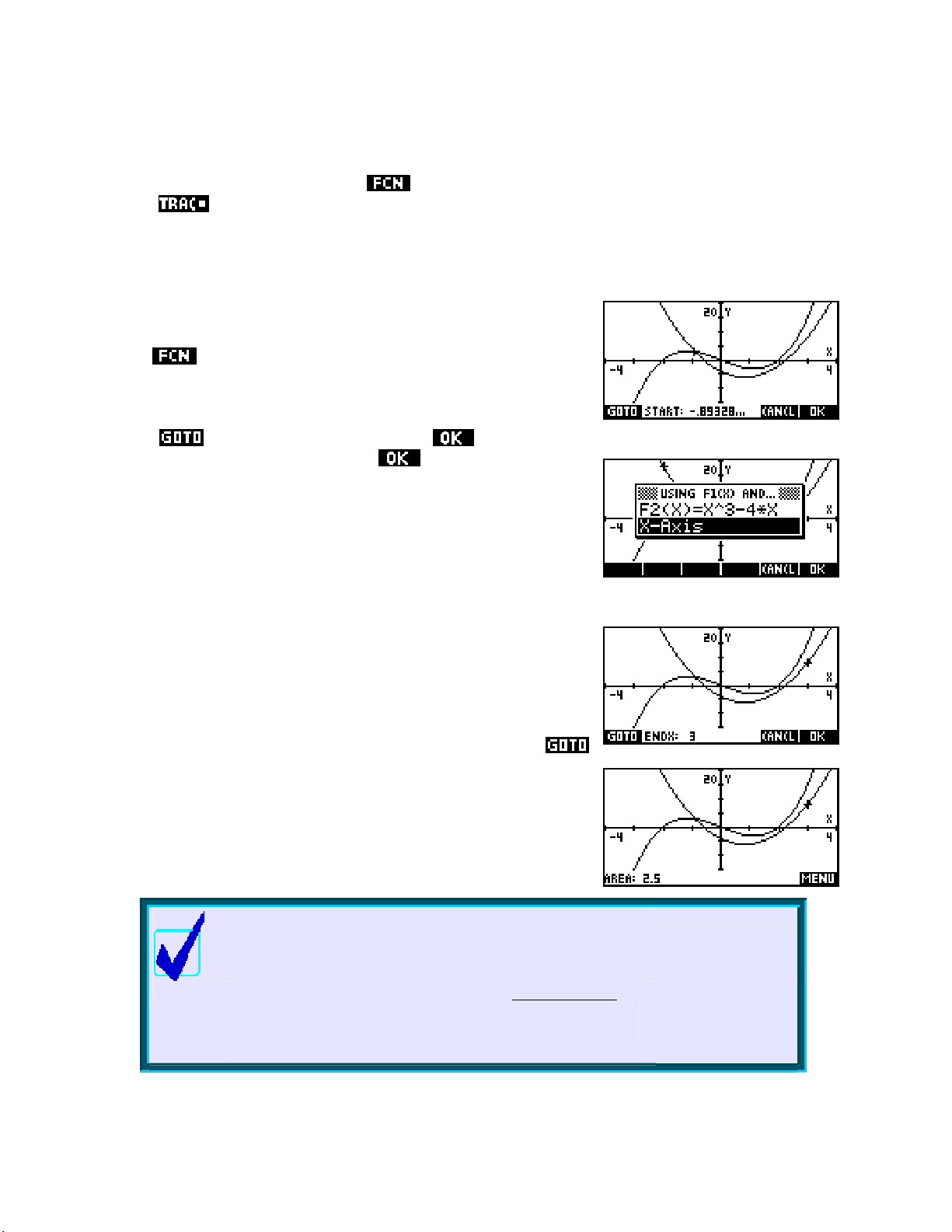
Signed area…

Another very useful tool provided in the sure that

is switched on, and that the cursor is on F1(X) - the quadratic. The Signed Area tool is

menu is the Signed Area tool. Before we begin to use it, make

similar to the Box Zoom in that it requires you to choose start and end points of the area to be calculated.

Definite integrals

Suppose we want to find the definite integral:

Choose

and then Signed Area. At the bottom of the screen you

− 5x − 4 dx

∫

−

will see a prompt, as shown right, asking you to choose a starting point.

Press the The starting value will then be -2 so press

key, enter the value -2 and press or ENTER.

again (or ENTER) to

accept it.

Another menu will now pop up, asking you to choose what area you wish to calculate. In this case there are only two choices: between

F1(X) and the x axis, or between F1(X) and F2(X).

If we had defined more functions in the would be longer. In this case we want the area between x axis, so position the highlight as shown and press

SYMB view then this menu

F1(X) and the

ENTER.

The graphs will then reappear, with a message requesting that you choose an end point. In the screenshot shown right I have pressed and entered the value 3 to move to that point directly.

If you now press

ENTER again to accept the end point, the hp 39gs or

hp 40gs will calculate the signed area and display the result at the bottom of the screen.

Calculator Tip

It should be c early understand that although the label at the bottom of the screen is

What has actually been calcu ated is the definite integral

it is a little misleading.

Area

l (right), with ‘areas’ below the x axis included as negatives. This is why the label on the original menu reads area” .

instead of just “Area”

“Signed

2nd point

∫

1st point

1( )

FX dx

Tracing the integral in PLOT

Rather than using the

key, an alternative method is to use the tracing facility. The advantage of this is that the ‘area’ is shown visually as you go by shading, as can be seen right.

The disadvantage of this is that you can only trace to values which are permitted in the scale you are using. As soon as you use

the shading stops. In this case, due to the scale we chose, if you try to trace to the values x = -3 or x = 2 you will find that they are not accessible. To illustrate the process we will need to change scale.

Change to the default values highlighting the

Press the left/right arrow keys or the

ENTER to accept the starting point.

Press

This time, choose the boundary as

PLOT SETUP view and set the x axis (only) back to the

-6.5 to 6.5, then PLOT again. This can be done by XRng fields and pressing DEL.

and again, choosing Signed Area… as before. Use

key to move the cursor to x = -2.

F2(X) instead of the x axis so that we

will be finding the signed area between curves instead of the signed area under one. Again, note that the result will be a signed area (definite integral) not a true area. See page

75 for a simple method of

finding true areas.

We now need to choose the end point. This time do it by tracing with right arrow to move the cursor. As you do the area will be shaded by the calculator. The current position is shown at the bottom of the screen. When you reach the end point you are looking for, press the

key and the area will be calculated as before. This is shown right. To remove the shading, press

PLOT again to force a re-drawing of the

screen.

Calculator Tip

Common sense tells us that the answer in the example above is almost certainl

y -3.75 rather than -3.75000000002. The small error is simply due to accumulated rounding error in the internal methods used by the calculator. as 0.5

For example, an answer of 0.4999999999 should be read

This is quite common and users should be aware of the need

for common sense interpretation.

Areas between and under curves

If we are wanting to find true areas rather than the ‘signed areas’ given by a simple definite integral then we must take into account any roots of the function.

The difficulty with this is that for most functions the roots and intersections are quite unlikely to be whole numbers and rounding them off will produce inaccuracies in the calculation.

There are ways to get around this and the process is shown in detail on page 75. Basically the trick is to find each root in turn and use the

HOME view to store the values of the roots as A, B, C… These values can then

be used in the calculation to retain full accuracy.

Extremum

The final item in the

menu is the Extremum tool. This is used to

find relative maxima and minima for the graphs.

Ensure that the cubic

F2(X) in the vicinity of the left hand maximum (turning point)

as shown right. Press

is switched on and that the cursor is positioned on

and choose Extremum from the menu. You

should find that the cursor will jump to the position of the maximum.

Calculator Tip

If your graph has asymptotes then make sure that the cursor is positioned on the side of the asymptote containing the extremum before initiating the process. The internal algorithm used does not cope well with intervening asymptotes.

Finding a suitable set of axes

This is probably the most frustrating aspect of graphical calculators for many users and there is unfortunately no simple answer. Part of the answer is to know your function – this is why we still expect you to learn mathematics instead of expecting the calculator to do it all! If you know, for example, that your function is hyperbolic then that immediately gives information about what to expect. If you don’t have knowledge then here are a few tips:

HHE

XXPPEERRT

•

Try plotting the function on the default axes. You may find that enough of the function is showing to give you a rough idea of how to ad either axis or on both. When in doubt, zoom out rather than in. See Tip #4 on the next page.

• The NUM view can be very helpful. Try changing to NUM SETUP and setting the value of

NumStep to 5 or even 10. Now scroll through the NUM view and look at what is happening to the F(X) values. Look for two things.

::W

o Firstly, where is the function most active? For what domain on the x axis is it changing rapidly

both up and down? This is likely to be the domain you are most interested in.

OORRKKIINNGGWWIITTH

UUNNCCTTIIOONNS

just them to display it better. Remember that

FFFFEECCTTIIVVEELLY

can work on

o Secondly, what is the range? What sort of values will you need to display on the y axis?

Change to the those you can

• If the graph is part of a test or an examination then the wording of the question will often give a clue

as to what x axis domain you should work with. You can then use Auto Scale.

Auto Scale can be used to get a first approximation to a good set of axes. To do this you must choose your x axis domain first. Use your knowledge of what the function might look like, perhaps together with a quick scroll through the

For example, suppose a company’s profit is modeled by the equation

number of items manufactured. Suppose that from the context of the question it is clear that we are mainly interested in the domain

After entering the equation into the

SETUP

steps of 10 (or 5 if you want more details).

view and set the numeric scale to start at zero and increment in

NUM view, to get an idea of what section of the x axis is important.

PLOT SETUP view and set what you think may be appropriate axes. From

PLOT and then zoom in or out.

0 ≤≤x 100 .

SYMB view, change into the NUM

()

−100

Px , where x is the

+ 50

−0.025 x

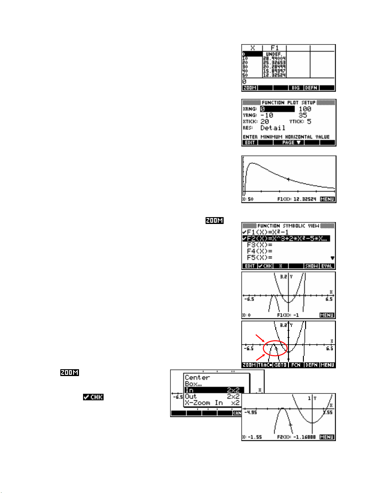
Change into the

NUM view and scroll through the window from zero to

100. As you do so, take note of the values that the function takes. From the display it seems that the function peaks around y=30 and then declines steadily.

Change into the

PLOT SETUP view and enter an x axis of 0 to 100

with a ‘tick’ value of 20, and a y axis of -10 to 35 with a tick value of 5.

The result of this is a

PLOT view as shown right. This would be ideal for

answering questions on the domain stated.

Another possible strategy for graphing which works quite well and, perhaps importantly, always gives ‘nice’ scales is to use

Enter your graphs into the

SYMB view. Remember that Auto Scale only

works on the first ticked graph.

VIEWS and choose Decimal, or press SHIFT CLEAR in the

Press

PLOT SETUP view. This will give you the default axes, probably not

showing the graph very well.

Place the cursor so that it is in the center of the area you are most interested in.

Use the

menu to adjust the view. You may choose first to change the zoom factors to something other than 4x4, and to ensure that Recenter is

ed. The PLOT view on the right is the result of setting 2x2 and recenter.

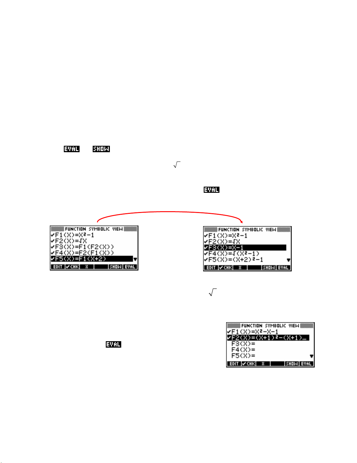
The advantage of doing it this way is that if you zoom in or out by a factor of 2 or 4 or 5, the cursor jumps

(

−

(

will stay at (relatively) nice values allowing you to trace more easily. In this case, the cursor now moves in jumps of 0 may not be important.

The disadvantage of this method is that you need to have at least some of the graph showing on the screen before you can zoom in or out to show more! Auto Scale can sometimes give you this first step.

Composite functions

05, which is ideal for most purposes. If you are not interested in tracing along the graph then this

The Function aplet is capable of dealing with composite functions such as

view. The

For example, if we define

F4(X). See the screen shot on the left below.

If the highlight is now positioned on each of these in turn, and the performed. The result is shown in the right hand snapshot.

Notice that the calculator is smart enough to realize in

not, unfortunately, smart enough to keep track of the implications for the domain, which are that be defined only for non-negative x.

and keys are particularly helpful with this.

1( ) =

Fx x 2 −1

and

2( x) =

x , then we can use these in our defining of F3(X),

F3(X) that

fx+2

key pressed then the substitution is

1 is the same as x − 1 , although

)

or fgx in its SYMB

)

(

()

)

F3(X) should

There is a limit to this however. If you define

2( ) = 1( Fx Fx +1) , then the routine will not simplify

x +1)− + −1 to x

(

x 1

(

)

+−1 .

Fx x x 11( )

−− and then

On the other hand there is a way to further simplify the expression.

the result and enclose it with the POLYFORM function as shown

right, adding a final ‘

,X’ as shown, then highlight it and press .

The calculator will expand the brackets and gather terms.

Calculator Tip

These functions can all be graphed but the speed of graphing is slowed if you don’t press This is because the composite function

first. is internally re-evaluated for each point graphed. The hp 39gs and hp 40gs are fast enough that the result is still satisfactory but if you have an old 39g or 40g they are slowed to the point of being unusable.

Evaluating the function may also hide the domain and for this reason it is sometimes best to leave the evaluation undone.

) =

For example, if

) = 1( 2(

3( X FFX )) will show the correct domain of x ≥ 0 for both

F2(X) and F3(X) in the NUM view. Pressing will destroy this.

1( X X

and

2( X) = X then

Using functions in the HOME view

Once functions have been defined in the

SYMB view of the Function aplet, they can be reused in the HOME

view (and indeed in any other aplet!).

For example suppose you needed to find some exact points (x = 0, 1, 2 and 3) for a graph

()

(

Type its definition into the Function aplet

HOME view and then simply type F1(0) and press ENTER. The

when doing a hand sketch of it.

x −

)

SYMB view, switch to the

function will be evaluated for x = 0. Similar results can be obtained for

F1(1), F1(2) and F1(3). Notice the error message for x = 2 caused by

a divide by zero.

A simpler way to get function values is to changing into the

NUM view and use its tabular listing.

Differentiating

−

There are different approaches that can be taken to differentiating, most of which are best done in the

SYMB view of the Function aplet.

The syntax of the differentiation function is:

∂X( function )

where function is defined in terms of X.

The function can be already defined in the

F2(X) in the screen shot above. Alternatively it can be directly entered into the brackets as shown in function F3(X).

∂ symbol most easily obtained by pressing the key

The labeled

. It can also be found in the MATH menu.

One point to remember is that if you use this function in the

SYMB view of the Function aplet as shown in functions F1(X) and

HOME view

you may not receive the result you expect. If you try this yourself your result will probably not be the same as that shown right.

The reason for this is that the result you see is the derivative of

evaluated at whatever value of x happens to be currently in memory. This can be seen more clearly if we store a specific value into the memory the value of the derivative

X beforehand. In the example shown right, the answer of 3 is

2x −1 at the value of x = 2.

But what of algebraic differentiation? It is possible but not very convenient to do this in the

S1. The drawback of this is simply the awkwardness of having to work

S1’s rather than with X’s.

with

HOME view using a “formal variable” of

Algebraic differentiation is most easily handled in the your function as

F1(X) and its derivative as F2(X) (see below)…

press

Calculator Tip

Doing your differentiation in the Function aplet is much easier and offers the additional advantage of being able to graph the two functions.

Circular functions

SYMB view of Function. The best method is to define

There are two issues that influence the graphing of circular functions, both related to the scale chosen.

The first one, illustrated on the right, causes circles to be ellipses if you don’t choose scales for the x and y axes which are ‘square’ relative to each other. The two graphs above are both

of the same function

x2 + y = 9 .

The simplest way to deal with this is to use scales which are multiples of the default scales. For example by using

6.2 y 6.4 − ≤≤

. These are a scale factor of 2 from the default axes of

13 x

−≤≤13 and

6.5 x 3.1 y 3.2 .− ≤≤6.5 and − ≤≤

You can also use the Square option on the

ZOOM menu. This adjusts the

y axis so that it is ‘square’ relative to whatever x axis you have chosen.

The second issue is caused by the domain of the circle being undefined for some values. The screen on your calculator is made up of small dots called pixels and is 131 pixels wide and 64 pixels high. As was mentioned earlier, this means that each pixel is 0.1 apart on the x and y axes.

This can affect your graphs and it becomes particularly obvious with circles because the graph does not exist for the part of the x axis outside the circle. The two screen shots right are an example of two images of

the same graph

x2 + =9 using two slightly different scales. You can see that the second example has y

missing pieces.

Let's look at the circle

x2 + =9 as an example. This circle only exists from -3 to 3 on the x axis and is y

undefined outside this domain. In order to graph it you have to rearrange it into two equations of:

F1(X)= (9-X

F2(X)= - (9-X

) for the top half

) for the bottom half.

If you enter these equations and then graph them with the default axes then you get a perfect circle. However, if you change the x axis to -6 to 6 rather that the default setting and then

PLOT again you will find

that part of the circle disappears. This is shown in the second snapshot above.

The reason for this is that when the calculator draws the graph it does so by ‘joining the dots’. For the default scale of -6.5 to 6.5 this is not a problem since the edges of the two half circles at -3 and 3 fall on a pixel. This means that the last segment of the graph plotted extends is from 2.9 to 3 and the circle reaches right down to the x axis.

However, for the scale of -6 to 6 the pixels are no longer 'nice' values of 0.1. If you try to trace the circle

you'll see that the pixels fall on 0, 0.0923077, 0.1846154..... In particular, near x=3 the pixel values are

2.953846 and 3.046154. This means that the calculator can't draw anything past 2.953846 because the next value doesn't exist, being outside the circle. This is what causes the gap in the circle. There's nothing to join to past that last point.

If this missing piece is a problem to you then the solution is to use scales which allow the end points of your circle to fall on a pixel point. If your circle has an integer radius then this is easily done by starting with the default axes and then

ZOOM in or out to show the circle. This will tend to give 'nice' pixel points. If your

circle is not centered on the origin then just check/tick the box in the Set Zoom Factors box to Recenter. That will allow you to turn off be and then

, move the cursor closer to the point where you'd like the centre of screen to

Trig functions

If you intend to

the graph of a trig function and you are using radian measure then you should choose a scale which will cause pixel values (screen dots) to fall at convenient points. A good scale to use is provided on the

This scale sets each dot to be

factors of

VIEWS menu (see right).

, ensuring that multiples and most

will fall on dots and thus helping if you want to trace values

on the graph. You can see in the example right that the value of

that the angle measure is set to Radians in the

MODES view if you intend to use this scale.

is easily traceable. You should ensure

Retaining calculated values

When you find an extremum or an intersection, the point is remembered until you move the cursor even if it is not actually on a value that would normally be accessible for the scale you have chosen.

For example, if you find an intersection and then immediately return to the

menu and choose Slope, the slope calculated will be for the intersection just found rather than for the nearest pixel point. If you have recently found a root then pressing the

key and entering the value Root will return the cursor to it.

There are two ways to access these values:

o The first and simplest is via the value stored in memory

HOME view without moving the cursor and type X then the value it will contain will be the last

X. If you move from the PLOT view to the

position of the cursor. If you just found a root or an intersection then this will be the value displayed. To find the y value for the x coordinate just evaluate

F1(X) in the HOME view (or whatever function

you are using).

o The second way is via the reserved words of

Root, Extremum, Area, Slope and Isect. Typing

any of these reserved words in any situation will retrieve their last calculated values. If a value has not yet been found then they will return zero.

This trick is particularly useful when calculating areas under or between curves. See page 75.

The NUM view revisited

We saw earlier that the

It is possible to manipulate this view through the

NUM view gives a tabular view of the function.

NUM SETUP view. The first way is to change the start value

and the step size for the view.

NumStart & NumStep

For example, values of 10 and 2 give:

Automatic vs. Build Your Own

Looking at the

NUM SETUP view you will see an entry called NumType with the default value of Automatic.

The alternative to Automatic is the setting of Build Your Own. Under this setting the waiting for you to enter your own values for

Typing in the values of (for example):

3 ENTER (-) 2 ENTER 5 ENTER

… will give…

NUM view will be empty,

In this situation the function values are being calculated as you input the

X values. This can be quite useful if

you are wanting to evaluate the behavior of a function at selected points.

ZOOM

If you now use the find that there is a

NUM SETUP view to switch to Automatic you will

key at the bottom left of the NUM view. This

can be quite useful as a fast way to reset the scale.

Pressing the

key pops up the menu on the right. The first option of In causes the step size to decrease from 0.1 to 0.025. This is a factor of 4 and is changeable via the

NUM SETUP view. I find a zoom

factor setting of 2 or 5 to be more useful.

The second option of Out causes the opposite effect, changing the step size upwards by whatever the Zoom Factor is set to.

The Decimal option restores the default settings. It changes from whatever is showing back to the step size of

0.1 The Integer option on the other hand, changes the scale so the step size is 1.

The Trig option changes the scale so that the step size is

exactly.

This will obviously be useful when dealing with trigonometric functions since it means that values such as

will appear exactly in the table.

Integration: The definite integral using the

∫

(

∫

The situation for integration is very similar to that of differentiation. As with differentiation, the results for algebraic integration are better in the Function aplet. The

The syntax of the integration function is:

(,, ,

a b function name )

∫

where: a and b are the limits of integration

and function is defined in terms of name. eg.

Let’s look first at the definite integral…

The screen left shows

∫

followed by

(1, 3,

∫

+1 dx = 3.3333…

ln 2

edx

∫

+ 5, x) or (0.5, π, cos ( S1 , S1)

= 1.

function

symbol is obtained via the keyboard.

)

It may help you to remember the syntax of the differentiation and integration functions if you realize that they are filled in with values in exactly the same way that they are spoken.

E.g.

& entered the same way:

A similar path was taken with the differentiation function, so that:

Note that although I have used

requirement. The integration example could be done as

+1 dx is read as:

∫

“the integral from 1 to 2 of

⎡

⎤

, which is read as “the derivative” ….. “with respect to X”…..“of X2”

⎦

⎣

and entered as it is read as

1 dx ”

( 1, 2, X2 + 1 , X )

∫

∂

X as the variable of integration in the examples above, this is not a

)

( 1, 2, A

1 , A ) with the same result.

Integration: The algebraic indefinite integral

(

Algebraic integration is also possible (for simple functions), in the following fashions:

• If done in the SYMB view of the Function aplet, then the integration must be done using the symbolic

variable there is no constant of integration ‘c’.

The screenshot right shows the results of defining

with the results of the same thing after pressing the (the result is placed in

All that is now necessary is to read ‘

or as it should be read as

• If done in the HOME view, then S1 must again be used

as the variable of integration.

S1 (or S2, S3, S4 or S5). If done in this manner then the results are satisfactory, except that

1( ) = SX

−1 and then

2( X) =

F3(X) only for convenience of viewing).

−+ .

0, 1,

∫

-S1+S1^3/3’ as −+

−1, X

, together FX X

)

key

i.e.

This is shown above, together with the results of highlighting the answer and pressing result may seem odd but is caused by calculator assuming that other variable and integrating accordingly as a ‘partial integration’. While mathematically correct, this is not what most of us want.

The way to simplify this answer to a better form is to highlight it,

right. This is the result of the calculator performing the substitutions implied in the previous expression.

−1 dx is entered as

∫

( 1, S1, X2 - 1, X ).

∫

it, and press ENTER again, giving the result shown

X itself may be a function of some

. The

A caveat when integrating symbolically…

∫

This substitution process has one implication which you need to be wary of and so it is worth examining the process in more detail. The expanded version of what is happening is shown below.

x−1dx

∫

⎡

⎢ ⎣

⎛

⎜ ⎝

= −S1

xS1

⎤

−

⎥

⎦

x= 0

3 3

−

1 3

⎞⎛

−

⎟⎜ ⎠⎝

⎞

−

⎟

⎠

The potential problem lies with the second line, where the substitution of zero results in the second bracket disappearing. This will not always happen.

For example…

x−2)dx

(

∫

⎡

⎢

⎣

(

⎜ ⎟⎜

⎜ ⎝ ⎠⎝⎠

(

= −⋅

x−2

(

−

S12

−

)

⎤

)

⎥ ⎥

⎦

x= 0

0 −2

(

)

⎞ ⎛ ⎟ ⎟

⎞⎛

)

−

⎟⎜

xS1

The final constant of 6.4 comes from substituting zero into the expression and should not be there if we were doing this with the aim of finding an indefinite integral. On the other hand, we all know that the answer should have a constant of integration, so perhaps this extra constant will help you to remember the ‘+c’!

Calculator Tip

There are strict limits to what the hp 39gs can integrate. For example, on the hp 39gs if you try to evaluate

able to do it.

Essentially, little beyond polynomials.

sin .cos it will not be

xdx

On the other hand, the hp 40gs is far more capable through its CAS (see page 324). The hp 40gs can handle integration by parts and by substitution as well as many other tricks.

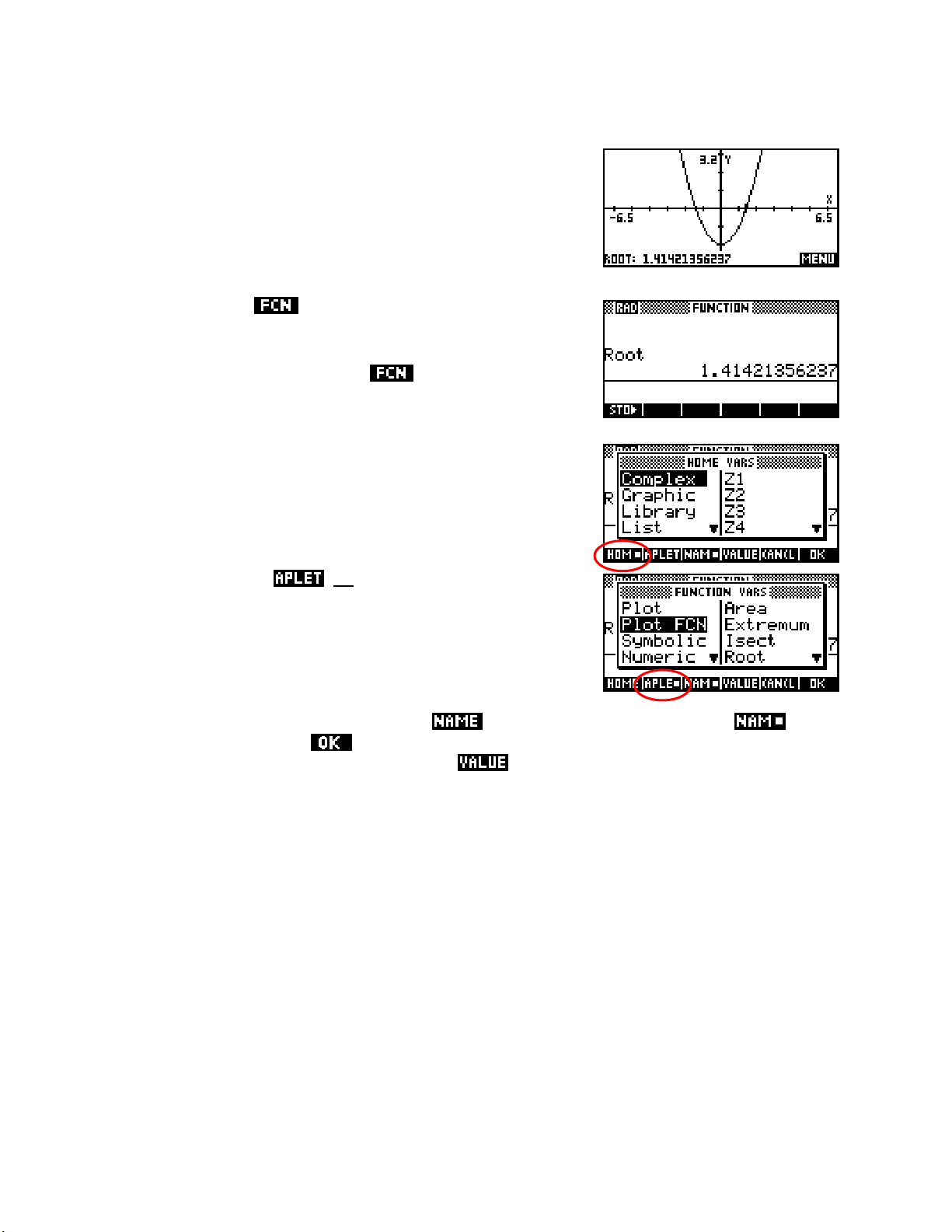
Integration: The definite integral using PLOT variables

As was discussed earlier, when you find roots, intersections, extrema or signed areas in the

PLOT view, the results are stored into variables for

later use.

For example, if we use

fx()= x2− 2

then the result is stored into a variable called Root, which

can be accessed anywhere else. Similar variables called

Extremum are stored for the other tools.

and

You can access these names by typing them in using the by using the

HOME variables.

If you press

VARS key. Press VARS and you will see a list of the

SK2, labeled

Root to find the x intercept of

Isect, Area,

ALPHA key, or

(not the APLET button on the keyboard), then the display changes to show the variables specific to whatever aplet you are currently using. Those shown right are for the Function aplet and the group of Plot FCN variables is shown.

If you look at the screen shot you will see that the this means that when you press using when you pressed the

VARS key. Pressing the screen key will cause the value of the variable to

the name of the variable will be pasted into what ever view you were

tag is currently selected (showing as ) and

be pasted instead. There is no effective difference in most situations.

This can be very useful in finding areas, as you will see in the example on the following page.

()= x2− 2 andSuppose we want to find the area between fx

−

() 0.5x −1

x =

graphs.

From the hand shaded screenshot shown above right it can be seen that to find the area we need to split it into two sections, with the boundaries being -2 and the two intersections.

After finding the first intersection using Intersection we change into the store the results into memory variable

We then do the same thing for the second intersection, storing the result into

from x = -2 to the first positive intersection of the two

HOME view and

We can now calculate the area in the

the first and

integral and edit it to adjust the functions and limits.

Finally,

− f

for the second. Use to duplicate the first

the two solutions and add them to give the final answer.

HOME view, using

for

Piecewise defined functions

It is possible to graph piecewise defined functions using the Function aplet, although it involves literally splitting the function into pieces.

x + 3 ; x <− 2

⎧ ⎪

For example:

fx()=⎨x2− 2 ; − 2≤ x ≤ 1

⎪

3−x ; x≥1

⎩

To graph this we need to enter it into the

SYMB view as

three separate functions:

F1(X)=(X+3)/(X < -2) F2(X)=(X2-2)/(X ≥ -2 AND X ≤  1) F3(X)=(3-X)/(X

Note: The

AND function can be found on top of the (-) key.

The reason why this works is that the

≥ 1)

(X < -2) and the (X ≥ 1) expressions are evaluated as being

-2 AND X ≤

either true (which for computers has a value of 1) or false (which has a value of 0).

By dividing by this domain expression we are effectively dividing by 1 inside the range (with no effect) or dividing by zero outside the domain (making the function undefined). This can be seen in the

NUM view to

the right. Since undefined values are not graphed, this produces the desired effect.

‘Nice’ scales

As discussed earlier, the reason for the seemingly strange default scale of -6.5 to 6.5 is to ensure that each dot on the screen is exactly 0.1 apart.

There are other scales, basically multiples of these numbers, that also give nice values if you want to along the graph. For example, halving each of -6.5 and 6.5 will place the dots

0.05 apart.

To zoom out instead of in simply double the values, producing dots that are 0.2 apart.

Similarly, if you want to center the graph around a particular value then just add that value to the range values. The example right is centered around x = 1 by adding 1 to -3.25 and 3.25.

Nice scales in the PLOT-TABLE view

A time when ‘nice’ scales are more important is when you use the PlotTable option in the

VIEWS menu. If you use the default axes you will

find that the dots, and hence the table values are no longer ‘nice’ because of the dots consumed by the line down the middle of the screen.

This can be solved by changing the x axis scale to -6.4 to 6.4, which gives table values of 0.2.

Using -3.2 to 3.2 is even better since it makes the graph ‘square’ again, with both axes proportional. Another good choice of scale for the Plot- Table view is -8 to 8, giving table values of 0.25. Basically any power of 2 is a good choice. Again, adding or subtracting a constant from each end of the axes will produce a graph where the y axis is not centred.

Use of brackets in functions

One problem commonly encountered by new users is misinterpretation of brackets. The hp calculator will correctly interpret

X2*(X+1) but will not understand F(X)=X(X+1). When used in either

F1(X) = X2(X+1) as

Function or Solve, it will result in the error message of “Invalid User Function”.

Similarly if you want to use the sum to n terms formula for a GP in the Solve aplet and enter it as message unless you change it to read

The reason for this apparent ‘error’ is that all of the built-in functions such as

ROUND(....) work with brackets. When the calculator encounters X(X+1) it interprets this as asking it to

evaluate a function called

S=A(1-R^N)/(1-R) then you will see a similar

S=A*(1-R^)/(1-R).

SIN(....) and COS(....) and

X(....) at the value X+1. Since there is no such function it returns the error message

that you are trying to use a function that is unknown.

The solution is simple: just remember to put the * sign in when you use letters immediately before a bracket.

Problems when evaluating limits

In evaluating limits to infinity using substitution, problems can be encountered if values are used which are too large.

For example:

lim

→∞

+ 6

It is possible to gain an idea of the value of this limit by entering the function

NUM view and then trying increasingly large values. As you can see

F1(X)=e^X/(2*e^X+6) into the Function aplet, changing to the

(right) the limit appears to be 0.5, which is correct. It is not the intention here to pretend that this is any sort of thorough mathematical justification but it does provide you with an indication of whether or not you are on the right track.

However, if you continue to use larger values then the limit appears to change to 1 (see right). This is obviously not correct, so why is it happening?

The reason for this is that the calculated value of e

500

calculator, which is 10

500

value of 10

) instead of the true situation of the bottom being roughly twice size of the top. This error is

. When this happens the top and bottom of the fraction become equal (both at a

very quickly passes the upper limit of the capacity of the

most likely to happen with limits involving power functions as they will overflow for smaller values of x.

The hp 40gs can instead evaluate limits algebraically using the CAS (see page

324). An

example is shown right to illustrate the results.

A related effect happens when investigating the behavior of the commonly used

⎛

calculus limit of

lim ⎜1

→∞

⎞

. One of the common tasks given to students in introductory calculus classes is

⎟

⎝

⎠

to evaluate this expression for increasing values of n to see that it tends towards e. This can easily be done in the Function aplet using the

NUM view but there is a trap in store for the unwary!

Begin as follows:

1. Entering the function into the

2. Change to the

NumType field.

in the

3. Now change to the

for

NUM SETUP view and choose Build Your Own

NUM view enter increasingly large values

The convergence towards e can also be seen graphically in the

SYMB view as F1(X)=(1+1/X)^X

PLOT view but is very slow to reach high

accuracy.

The ‘trap’ mentioned earlier lies in the fact that the slow convergence will mean that people will often try to graph this function for very large values of

X. The first graph on the

right shows the graph of this function for the domain of 0 to 100. The second graph shows how instability develops in the domain 0

110

to 1E11 (

).×

This apparent instability is caused by the internal rounding of the calculator. It works to 16 bits accuracy, which means that it can store 12 significant digits (for reasons only of interest to programmers). This means that when you invert a really large number and add it to one, you lose a lot of accuracy.

For example, if X =

⋅× ⋅ ×

285 10

then 1/

is 2 5087719298 10

-11

. When you add 1 to this, the calculator is

forced to discard all but the last decimal place because it can only store 12 significant digits. Thus 1 + 1/ becomes 1.00000000003 (rounded off from 1.00000000002508...)

There are naturally a whole range of numbers which will all round off to the same value of 1.00000000003, so that (for that range of numbers)

the expression (1+1/X)

is equivalent mathematically (on the HP) to

1.00000000003X. This produces a short section of an exponential graph, which only looks linear because you don't see enough of it.

Eventually the calculator reaches a value on the x axis which is large enough that it rounds off to a smaller number than 1.00000000003, which is 1.00000000002. This produces the sudden drop in the graph as

the plot changes from a section of a 1.00000000003

graph to a section of a 1.00000000002X graph

(which has a shallower gradient).

This section is maintained until the next drop, and so on. Finally, at the value x =

210

the inverted value is ×

so small that 1+1/X becomes exactly 1 and the graph becomes horizontal. Of course this is completely the wrong value!

Although this explanation may be beyond the level of many students it is quite important that they have some understanding of these ideas if they use an hp 39gs to numerically evaluate limits. Because of the CAS on the hp 40gs this situation is less likely to be a problem for that model. The solution to all problems of this type is to simply be aware of their existence and to allow for them rather than simply accepting the results shown in

NUM view.

the

Gradient at a point as the limit of the slope of a chord

The true gradient at a point is available in a number of ways. For example, via the

PLOT view or via the δ differentiation operator. For students first being introduced to calculus a common task

is to investigate the slope of the chord joining two points as the length of the chord tends towards zero.

xh fx

+)−

⎛

ie.

This can be effectively introduced via the Function aplet.

Begin by entering the function being studied into

To examine the gradient at x=3, store 3 into memory A in the view as shown right.

Return to the expression:

lim

h→0

SYMB view, un- the function F1(X) and enter the

F2(X)=(F1(A+X)-F1(A))/X in F2(X).

(

⎜ ⎟ ⎝

⎞

)

(

⎠

F1(X) as shown.

HOME

Slope tool in the

This is the basic differentiation formula quoted above with role of h and

Change to the Your Own”. By entering successively smaller values for investigate the limit as h tends towards zero.

In this case it is clear that the limit for x=3 is the value 6.

To investigate the gradient at a different point simply change back to the

HOME view, enter a new value into A and then return to the NUM view.

The disadvantage of the previous method is that it is not very visual. An alternative is to use an aplet downloaded from the web. An aplet that will automate the process and provide a visual display of the chord diminishing in length can be found on the author’s website at

http://www.hphomeview.com

A being the point of evaluation, in this case with A = 3.

NUM SETUP view and change the NumType to “Build

X taking the

X you can now

Finding and accessing polynomial roots

POLYROOT function can be used to find roots very quickly, but the results are often difficult to see in the

The

HOME view due to the number of decimal places spilling off the edge of the screen, particularly if they

include complex roots. This can be dealt with easily by storing the results to a matrix.

()= x3− 3x + 3 .

For example, suppose we want to find the roots of We will use the

POLYROOT function and store the results into M1.

The advantage of this is that you can now view the roots by changing to the

Matrix Catalog (SHIFT 4) and

pressing

. See page 209 for

more detailed information on matrices.

In addition to this, you can access the roots in the

HOME

view as shown. This method works equally well for complex roots.

See page 309 for details on finding roots of real and complex polynomials using the CAS on the hp 40gs.

Calculator Tip

This trick is particularly helpful if you are working with complex roots. Not only does it make it easier to re-use them it makes it easier to tell at a glance which are real and which complex.

HHE

In addition to the views of PLOT, SYMB and NUM (together with their SETUP views), there is another key which we have so far only used very fleetingly - the

It may seem odd to devote an entire chapter to what might appear to be an inconsequential key. In fact, however, this button is very useful to the effective use of the calculator, and crucial if you intend to use aplets downloaded from the internet.

The contents of the Function aplet contents are covered here but the others differ in only small ways.

Aplets downloaded from the Internet, however, will usually have a radically different program for the aplet. See page process if you intend to program the calculator. The first image shown right shows the contents of the Toss” which investigates probability.

WSS

VVIIEEW

MMEENNU

VIEWS menu changes slightly according to which aplet you are currently using. The

VIEWS menus created by the person who wrote the

VIEWS key.

257 for more information on this

VIEWS menu for an aplet called “Coin

VIEWS key normally pops up the menu on the right. We have

The already seen the use of the Auto Scale option (see page probably the one most used. The other options are also very useful at times.

1( ) =

Shown on the right is the graph of

VIEWS key, the menu above will pop up.

On the pages following we will investigate each of the menu options in detail.

FX X2 −1 . If we press the

89) and this is

Plot-Detail

Choosing Plot-Detail from the menu splits the screen into two halves and re-plots the graph in each half. The right hand side can now be used to

without affecting the left screen. The idea is that you on

the left screen and the result appears on the right screen.

For example a Box zoom shows the result on the right allowing easy comparison of ‘before’ and ‘after’ views.

The left hand graph is always the active one, with results of actions shown on the right. We can now use the left graph again to zoom in on another section of interest, or alternatively, press the key under the label. This switches the right hand graph onto the left screen so that you can perform progressive zooms.

ll the normal function tools are

available except .

Using

or the menu you can then find or examine points of interest. Alternatively you can zoom in again using another Box zoom.

Any of the normal

tools such as Signed Area or Extremum can

be used in this split screen.

Plot-Table

The next item on the

VIEWS menu is Plot-Table. This option plots the

graph on the right, with the Numeric view on the right half screen. Using the left/right arrow keys moves the cursor in both the graph and the numeric windows.

See page 79 for information on how to keep nice

scales in the table view. When more than one function defined in the

SYMB view, pressing the up or down arrows changes the table focus

from one to another. In this case, with only one, it centers the table.

1( )

Let us switch now to a graph of the two functions

FX X − 52( ) = 3 + 2 X X − 4 . This is shown on the right, using an XRng

FX X 2 −1 and

of -8 to 8.

Choosing Plot-Table gives the result shown left. As you can see, the scale has been preserved unchanged, although without labels. The table

on the right also uses a sensible scale of 0 an x axis scale of -8 to 8. As mentioned, choice of scale in the

Table

view is discussed in detail on page 79. The technique is requires

slightly different values than the default values in the

25 because of the choice of

Plot-

PLOT SETUP

view.

Looking at the table heading you will see that it currently shows the function

F1(X). The left/right arrow keys move within that function, with

the cursor keeping track. Pressing the up/down arrows now not only centers the table highlight but, more importantly switches from

F2(X). The X column does not change.

F1(X) to

Nice table values

What makes this view even more useful is that the table keeps its ‘nice’ scale even while the usual

tools are being used. As you can see in the screenshot left, the table is automatically repositioned to show the closest pixel value to that of the extremum found.

The Signed Area tool is also available in this view and when the cursor is moved the values in the table follow it. Unfortunately, the highlighted value in the table doesn’t change as the cursor moves to create the shaded area.

For this reason the best strategy is to use the

key to jump

to the end point. This means that the area will not be shaded but this should not be a problem.

Overlay Plot

Another possibility from the

VIEWS menu is Overlay Plot. This option can be used to add another graph

over the top of an existing one, without the screen being blanked first as it usually is. As an example, if you have already graphed functions

F1(X) through to F6(X) SYMB view, then

you may not want to have to wait while all the earlier ones are redrawn.

and then add another one in the

If you un-

the earlier graphs and then use Overlay Plot for the new one then it will be drawn over the top of the existing ones. Of course the results will not be good if the scales don’t match!.

More usefully, you can use this to combine different styles of graphs. For example, the screen shot right was produced by drawing a circle in the Parametric aplet and then superimposing the equations y = x and y = -x in the Function aplet. This could be used to show, for example, the enclosing curves for conic sections.

You can also use this technique to overlay functions on top of statistical graphs. Again, the important point would be to ensure that the scales matched.

Auto Scale

−

Auto Scale is an good way to ensure that you get a reasonable picture of the graph if you are not sure in advance of the scale. After using Auto Scale you can then use the

PLOT SETUP view to adjust the results.

It is important to understand two points about how Auto Scale works.

1. Auto Scale uses the X-axis range that is currently chosen in

range to include as much of the graph as possible. It will not adjust the x axis.

first

2. Auto Scale is done only for the

graph with a . If there are other graphs and they don’t fit the scale then they will not benefit. As you can see in the example shown right, the quadratic shows well but the second graph (a cubic) shows only an ascending section. Zooming out would be an option at this stage, as would un-

ing the quadratic in the hopes that

Auto Scaling the cubic might give better results.

The resulting y scale is often not a very ‘nice’ one. Commonly you will find that the y axis appears ‘thick’ as shown right. The reason for this is that the

Ytick value is too small, resulting in ticks too close

together.

You will usually have to adjust it in the make it look good. The third graph has a

PLOT SETUP view to

Ytick value of 10

instead of 1.

PLOT SETUP. It then adjusts the Y-axis

Decimal, Integer & Trig

The next option of Decimal resets the scales so that each pixel (dot on the screen) is exactly 0

−⋅ ≤ ≤ ⋅

and a Y scale of

31 y 32

1. The result is an X scale of . This may not give the best view of the

⋅≤ ≤ ⋅ 65 x 65

function. Personally I don’t often use it, as it is generally easier to go to

PLOT SETUP view and press SHIFT CLEAR, which restores the

the factory settings to all fields.

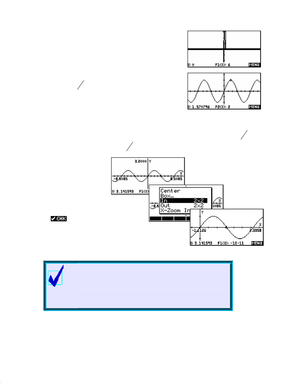
The Integer option is similar to decimal, except that it sets the axes so

that each pixel is 1 rather than 0.1 thus giving an X scale of

−≤ X ≤ 65 . The usual result of this is rather horrible to be honest.

The final option of Trig is designed for graphing trig functions. It sets the

scale so each pixel is

F1(X)=2SIN(X) then pressing the left or right arrow 24 times would

move you through exactly

. This means that if you were graphing

and the value would be exactly 2 instead

of a horrible decimal. This is shown right.

If you zoom in or out from this, the jumps will still stay relatively nice, particularly since 24 has so many

factors. For example, with a zoom factor of 2, zooming out once would mean each pixel was now

while zooming in would give a pixel jump of

The default axes under the Trig

−2

option is primarily interested in the first 2

to 2π . If you are

π of

the graph then simply change Xmin to zero. Alternatively you can move the cursor to

(the middle) and

then zoom in.

The example right uses zoom factors of 2x2 with

Recenter:

ed.

Calculator Tip

In the graphs above the cursor is at x = . The coordinates at the bottom of the screen should show F1(X)=0 but doesn’t due to the fact that the value of π rounding of decimal place means that the resulting trig

stored internally is not exact and of course cannot be. The

π in the 13

values will be ‘wrong’ in the 11 decimal place depending on the function used.

to 15

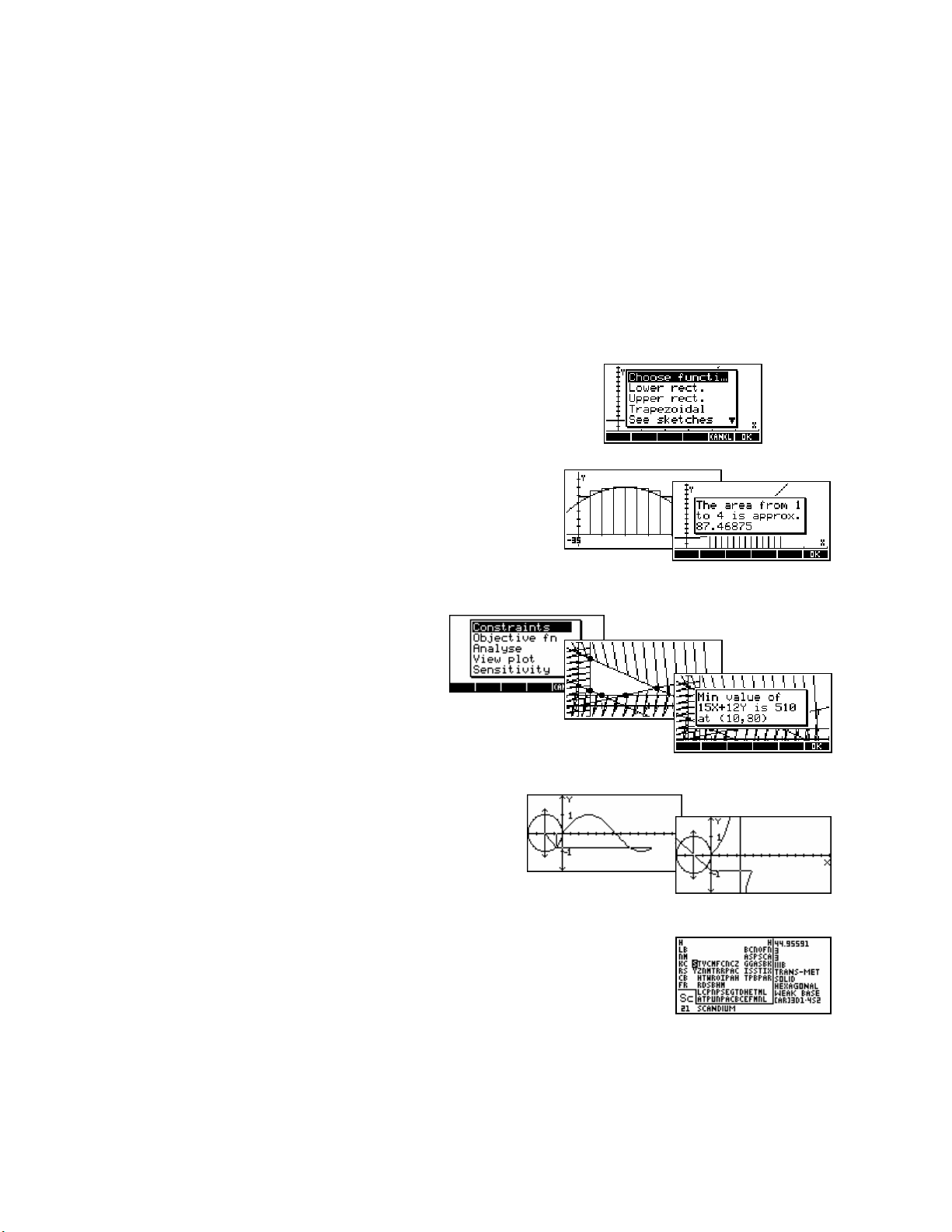
DDoowwnnllooaaddeeddAApplleettssffrroommtthheeIInntteerrnneet

The most powerful feature of the hp 39gs & hp 40gs is that you can download aplets and programs from the internet to help you to learn and to do mathematics. Two quick examples of aplets that are available are shown here. More are listed in the supplementary appendix on “Teaching Calculus using the hp 39gs & hp 40gs” and examples are also given in the chapter on programming. In each case the aplet is controlled by a menu. This menu is created by the programmer and ‘attached’ to the place of the normal menu.

Curve Areas

This aplet allows the user to find approximations to the area under a curve by finding either the lower rectangular area, the upper rectangular area, or the trapezoidal area.

The user can choose the end points of the interval, the type of calculation and the number of rectangles to be used. The rectangles are drawn on the screen. A worksheet introduces the idea of integration to find areas.

VIEWS button so that it displays in

Linear Programming

This aplet visually solves linear programming problems, finding the vertices of the feasible region and the max/min of an objective function. It even performs sensitivity analysis on the collected vertices.

Sine Define

This is an aplet to illustrate the process of obtaining the sine, cosine & tangent graphs from the unit circle.

Periodic Table

This is a library that can be added to the calculator which allows the user to display a periodic table with information on each element.

This aplet is used to graph functions where x and y are both functions of a third independent variable T. It is generally very similar to the Function aplet and so we will look mainly at the ways that it differs.

An example of a graph from this aplet is:

Although you can graph equations of this type, only some of the usual see in the screen shot above, the Thinking about the nature of these equations will tell you why.

As usual the first step is to choose the aplet in the Aplet Library. Press the ensure that you see the same thing as the examples following then press the

As with the Function aplet, this aplet begins in the view by allowing you to enter functions, but the functions are X and another for Y.

HHE

xt t yt

AARRAAMMEETTRRIIC

() =5cos

() =3sin 3

APLET key, highlight Parametric and press . If you wish to

paired

⎫

()

⎪

⎬

()

⎪

⎭

button before pressing .

. Each function consists of a function in T for

≤≤

PPLLEET

which gives:

key is not shown, meaning that none of its tools are available.

PLOT tools are present. As you can

SYMB

Choose XRng, YRng & TRng

Looking at the enter a range for T as well as the usual ranges for X and Y. It is crucial to understand the different effect of the T range to that of the X and Y ranges.

PLOT SETUP view, you will see that we now have to

Calculator Tips

i. The default setting for TStep is 0.1. In my experience this is too

large and can result in graphs that are not sufficiently smooth. It is worth developing the habit of changing it to 0.05

ii. The default maximum for T is 12. If your graph involves a trig

function then this may not be a good choice. A better one might be 2π. You can use the pi above the button to enter this.

The effect of TRng

≤

The X and Y ranges control the lengths of the axes. They determine how much of the function, when drawn, will be visible.

See the examples below. Notice that in both cases,

is on and shows the T value,

followed by an ordered pair giving (X,Y).

gives a graph of:

whereas..

gives a graph of:

XRng & YRng, the effect of TRng is to decide how much of the graph is drawn at all, not how much

Unlike is displayed of the total picture.

For example…

gives a graph of:

As you can see above, changing the T range from

0 ≤t ≤ 2

to 0

t ≤ 5 gives a graph that appears only

partially drawn. Of course, what constitutes “fully drawn” depends on the function used.

TStep controls smoothness

The value of the parameter values of

T when evaluating the function for graphing. Making TStep

TStep controls the jump between successive

too large will produces a graph which is not smooth. The example on the right shows

TStep=0.5 instead of 0.05.

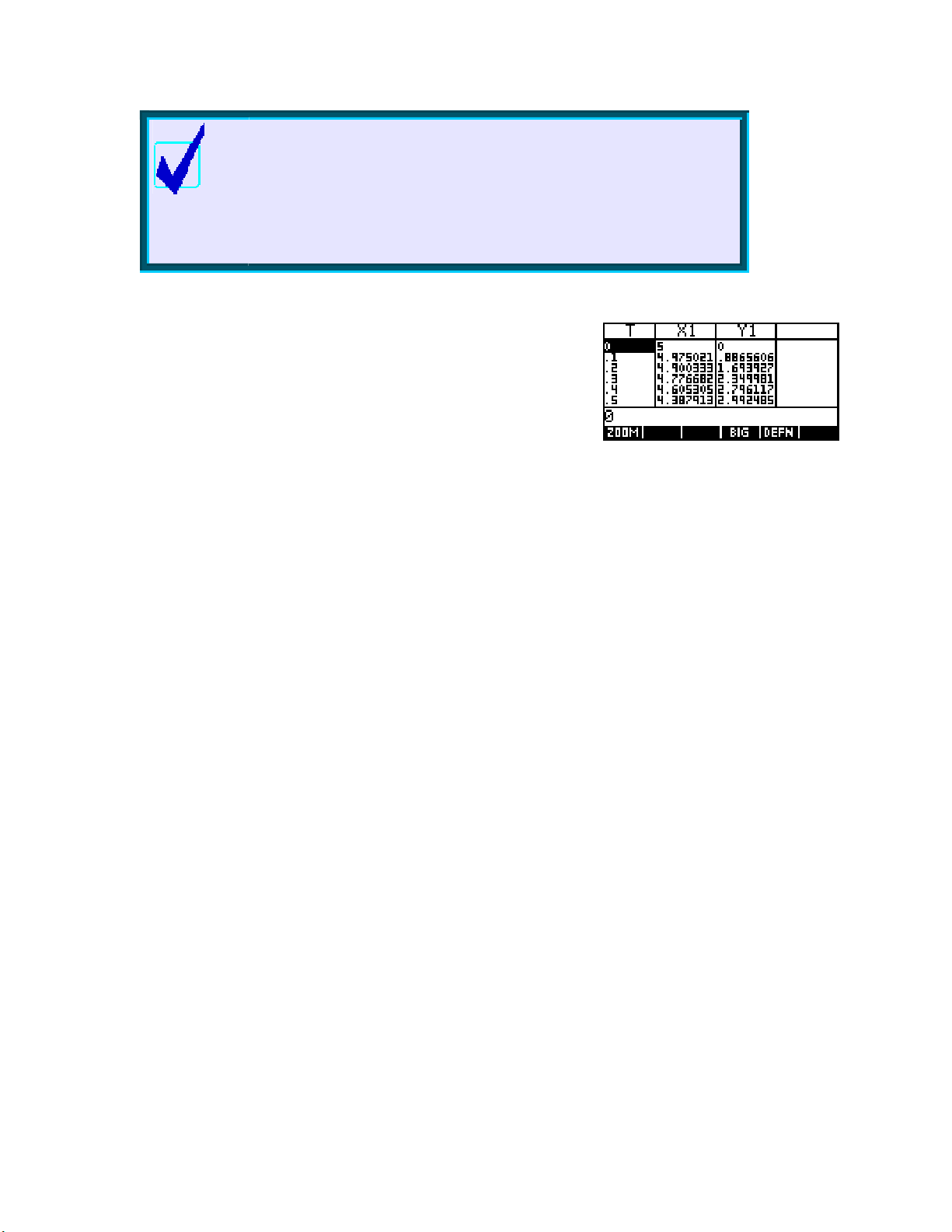
Calculator Tip

 TStep

Decreasing beyond a certain point will slow down the

graphing process without smoothing the graph any further.

0.05 is generally enough.



Since trig functions are often used in parametric equations, one

should always be careful that the angle measure chosen in

MODES l

is correct. The defau t for all aplets is radian measure.

As usual, the NUM view gives a tabular view of the function. In this case there are three columns, since

X1 and Y1 both derive from T.

As with the Function aplet, it is possible to change the starting point and step size of the table, and also to change it into a Build Your Own type of table (see page 70).

Using

HE E

XXPPEERRT

FFuunnaannddggaammees

Apart from the normal mathematical and engineering applications of parametric equations, some interesting graphs are available through this aplet. Three quick examples are given below.

Example 1

Try exploring variants of the graph of:

()

Example 2

Try varying the values of A and B in the equations:

1(t) = ( A B)cos(t Bcos((

1( + ) −

= 3sin 3t

= 2sin 4t yt

) =(

EECCTTOOR

::V

+ ) −

)sin(

A B

t B

UUNNCCTTIIOONNS

+1) )

sin((

+1) )

Hint: An easy way to vary A and B is to store values to memories

equations exactly as shown. New graphs can then be created by changing back to storing different values to

TRng of 0 to 31.5 step .2, XRng of -21.66 to 21.66 and YRng of -12 to 9. It also has Axes

un-

Example 2

Try varying the constants in the equations:

’d in PLOT SETUP.

A and B. The example shown uses A=4, B=2.5 and has axes set with

A and B in the HOME view and enter the

1(t) =3sin(t) +2sin(15 t)

yt) = 3cos(t) + 2cos(15t)

For those who remember them, this is curve like those produced by a “Spirograph”.

HOME and

VVeeccttoorrs

The Parametric aplet can be used to visually display vector motion in one and two dimensions.

Example 1

-1

A particle P is moving in a straight line. Its velocity v (in ms

()= 2t − 5t2+ 2t − 3

. Illustrate its motion during the first 2.5 seconds.

) at any time t (in seconds, t>0) is given

Enter the motion equation from (v) as X(T) and enter Y(T)=T. The only purpose of this second equation is to move the particle up the y axis as it traces out its path, thereby making it easier to view.

Changing to the

NUM view lets me scroll through the first three seconds

of movement, allowing me to choose a good scale for the x axis.

I’m interested in the first 2½ seconds only, so I’ll also restrict TRng to 0 to 2.5. Using Y(T)=T for this TRng means the y values will also range from 0 to 2.5. Maximizing visibility of this range of values is the reason for setting YRng to be –0.5 to 3 in axis is chosen from the values shown in the

PLOT SETUP. The range for the x

NUM view . The value of

TStep is carefully chosen so that when the motion plots, the speed is slow enough to show its progress.

The graph makes it plain that it doubles back twice in the first two seconds. The really nice part about this method though is that the motion can be seen on the screen. As the particle slows down near the turning points it does so on the screen. As it accelerates in the final section you can see this on the screen too. Obviously this can’t be seen on this page, and I recommend you try this for yourself.

Example 2

Two ships are traveling according to the vector motions given below, where time is in hours and distance in kilometers. Illustrate their motion during the first ten hours.

100

−

Ship A

Ship B

Enter the equations of motion as shown right.

Now change to the values. Possible values are shown below.

Now press example, the value of graph appears it can be seen that the ships do not collide, even though the final plot may make it appear that they do.

PLOT SETUP view and set the axes to suitable

PLOT to see the ships paths appear. As with the previous

TStep is chosen to allow visible motion. As the

⎛

x =

⎜

500

⎝

200

⎛



= +

⎞⎛

⎜⎟⎜ ⎟

400

⎝

⎠⎝

⎞⎛

+ t

⎟⎜ ⎟ ⎠⎝

−

⎞

⎞ ⎠

−

⎠

To find the distance between the two ships at any time t, you can enter

the equation

Function aplet. Note that the active variable must be an X in the Function aplet instead of the T of the Parametric aplet but you can still refer to the Parametric functions this function in the its minimum value. In this case the minimum separation of 13.74 km is achieved at t=8.68 hrs.

F1(X)=

(X1()

X1 and Y1 even within the Function aplet. Graphing

PLOT view of the Function aplet will allow you to find

− X 2

())+(

Y X X 1

()

− Y2

())

into the

≤

This aplet is used to graph functions of the type where the radius r is a function of the angle the Parametric aplet, it is very similar to the Function aplet and so the space devoted to it here is limited mainly to the way it differs. Some examples of functions of this type, together with their graphs are:

Choose XRng, YRng &

The

X and Y but for θ. The values set for XRng and YRng control the length

of the axes. The movement of the cursor follows the increments set for in

The values of

θRng control how much of the graph is drawn, while the values for XRng and YRng only control how much

of the graph is displayed on the screen once drawn. in the Parametric aplet. The default values for

HHE

θStep regardless of the resulting X and Y positions.

Step and smoothness

OOLLAAR

R1(θ) = 4 cos(3θ) R2(θ) =0.5

PLOT SETUP view shows that ranges must be specified not only for

θRng and for θStep are critical in controlling the appearance of the graph. The values set for

PPLLEET

Rng

θStep controls how smooth the graph is, as did TStep

θRng are 0

θ (theta). As with

≤ 2

and the default value for θStep is π/24.

R3(θ) =+3 2 sin(10θ)

Changing the default for

The default for between smoothness & speed. If you particularly want to use a fraction of

try

Circular circles

If it is important that graphs of circles do not look oval, then use the default values for the axes. If the resulting axes don’t show enough of the function, then be used to achieve round circles.

θStep often results in graphs which are not very smooth and 0.05 is a better compromise

Step

in or out. The Square option can also

π to aid in tracing the graph then

}

{

}

This aplet is used to deal with sequences, and indirectly series, in both non-recursive form (where T function of n) and implicit/recursive/iterative form (where T

Recursive or non-recursive

Examples of these types of sequences are:

As with most aplets, the Sequence aplet starts in the you enter formulas. The Sequence aplet uses the terminology U(N) rather than the other commonly used T avoid having to use subscripts which would not show up well on the screen.

HHE

EEQQUUEENNCCE

(explicit/non-recursive)

T = 3n −1 ..... {2, 5,8,11,14,.....

T = n

T = 2 ..... {2, 4,8,16, 32,.....

(implicit/recursive)

T = 2T

T =T

n−1

=−

n n−1

n n−1 n−2

T ;T

..... {1, 4, 9,16, 25,.....

PPLLEET

}

−1 ;T1 = 2 .....

2 ..... {2, 3, 2, 3, 2,.....

T ;T

1,T

1 ..... {1,1, 2, 3, 5,8.....

for its definitions in order to

is a function of T

2, 3, 5, 9,17,.....

} }

SYMB view when

n-1

is a

All functions of this type are assumed to be defined for the positive integers only – ie. for

First, second & general terms

Each definition has three entries -

U1(N) (see above) but it is not always necessary to

supply all three.

For example, if the sequence is non-recursive then only the needs to be filled in, with the other two entries calculated automatically from the definition as shown in the sequence of two screens shown right.

N = 1,2,3,4…

U1(1), U1(2) and

U1(N) entry

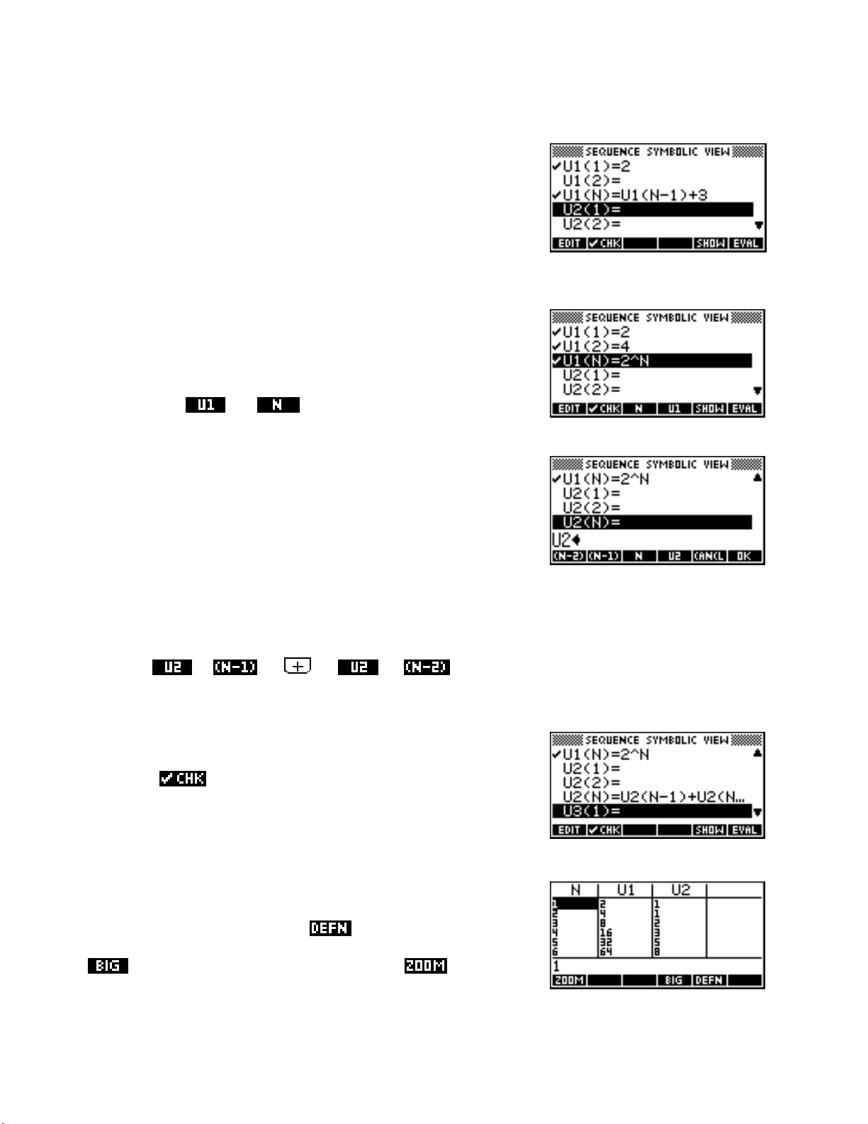
If the definition is recursive but only involves value for

For example, for the sequence enter the value

The value of calculator automatically in the

U1(2).

= T

n−1

5 into U1(1) and the expression U1(N-1)+4 into U1(N).

U1(2) will be ignored in the SYMB view but filled in by the

NUM view.

rather than both T

n−1

+ 3; T1 = 2 you need only

Convenient screen keys provided

There are a number of very convenient extra buttons provided at the bottom of the screen when entering sequences.

n−1

and T

then you need not enter a

n−2

Two of these moves onto the

and

U(N) line (see right). Pressing either will enter the

- are available as soon as the cursor

appropriate text into the sequence definition.

The rest become visible once you have begun to enter the sequence definition.

For example, suppose we enter the Fibonacci sequence into

U2 by defining U2(N) as U2(N-1) + U2(N-2).

Rather than having to type all of this we can use the buttons provided, pressing:

This is a very convenient feature, and worth remembering.

There is no defined recursively and no values have yet been given for

U2(2). Type in a value of 1 for both of these and then press the NUM

button to switch to the

mark next to the definition yet, since the sequence is

U2(1) and

NUM view.

As you can see in the screenshot right, the values in the sequence as a table. If you move the highlight into the

U2 columns, you can press the button and see the sequence

and

NUM view shows the actual

rule. You can experiment for yourself and see the result of pressing the

button (see next page for an example). The

button is also

available as usual, but it is easier to use other methods.

100

HP 39gs Graphing Calculator, 40gs Graphing Calculator User Manual

Specifications and Main Features

Frequently Asked Questions

User Manual

The hp 39gs vs. the hp 40gs

The SHIFT and ALPHA keys

The ALPHA key

The Screen keys

Pop-up menus & short-cuts

The Finance aplet (see page 155)

The Function aplet (see page 46)

The Inference aplet (see page 141)

The Linear Solver aplet (see page 150 )

The Parametric aplet (see page 92)

The Polar aplet (see page 98)

The Quadratic Explorer aplet (see page 159)

The Sequence aplet (see page 99)

The Solve aplet (see page 105)

The Statistics aplet (see page 114 & 123)

The Triangle Solve aplet (see page 152 )

The Trig Explorer aplet (see page 162)

Some typical aplet views

The screen keys

Aplet related keys

The arrow keys

The SYMB, PLOT and NUM keys

Intro to the VIEWS menu

The VARS key

The SETUP views

The MODES view

Numeric formats

The ANS key

The negative key

The CHARS key

The DEL and CLEAR keys

The MEMORY MANAGER view

Downloaded aplets & memory

The GRAPHICS MANAGER

The LIBRARY MANAGER

Pitfalls in Fraction mode

COPYing calculations

Clearing the History

SHOWing results

Choose the aplet

The SYMB view

ing your function

The NUM view

The PLOT view

In the down to Auto Scale and press

Detail vs. Faster

Simultaneous

Connect

Axes

Labels

Grid

The MENU toggle

Trace

Defn

Goto

The Zoom Sub-menu

Center

In/Out

Box…

X-Zoom In/Out x4 and Y-Zoom In/Out x4

Square

Auto Scale, Decimal, Integer and Trig

Root

Intersection

Slope

Signed area…

Definite integrals

Tracing the integral in PLOT

Areas between and under curves

Extremum

Finding a suitable set of axes

Composite functions

Using functions in the HOME view

Differentiating

Circular functions

Trig functions