

Page 1

Remote programming
and measuring
uncommon RTDs with
the Fluke 726
Using custom RTD temperature constants
The Fluke 726 Multifunction Process Calibrator can
measure temperature with most common resistance
temperature detectors (RTD’s). But what about the many
“legacy” non-standard RTD’s still in use, as well as standard
RTDs that have been specially calibrated? The 726 allows
you to enter custom RTD constants so you can measure
any RTD for which you have the constants. You can also
use custom constants to take advantage of the Fluke 726
ability to measure with 0.01° resolutions by coupling it with
a characterized RTD. This application note explains how
to use the 726 to measure non-standard or characterized
RTD’s. It covers the basic theory of RTD conversion formulas and shows how to load custom constants into the Fluke
726 using a Windows PC with an RS-232 serial port.
Application Note
RTD Temperature Curves
RTD’s take advantage of a natural property of
metals, namely that a metal’s resistance increases
with temperature. An RTD is a precisely manufactured metal wire or film, and by measuring its
resistance we can derive its temperature.
Resistance of an RTD is a function of the length
and cross sectional area of the wire or film used to
make it, and the resistivity of its metal. Resistivity
is a characteristic of a metal’s chemical makeup.
Most RTD’s are made of platinum, nickel, or copper.
The alloy of the platinum or copper must be tightly
controlled to produce precise resistivity. International standards like IEC 60751 and ASTM 1137
define the geometry and resistivity of standard
RTD’s. RTD manufacturers work to build their product to meet these standards.
In addition to defining the physical parameters of
standard RTD’s, international standards also define
equations and constants used to convert resistance
readings to temperature. Over a limited range the
relationship between temperature and resistance is
approximately linear, and you can convert temperature to resistance using Equation 1.
Equation 1: R
Where: t is the temperature of the sensor
R
a is a constant slope that describes
R
Using this simple linear equation delivers fairly
good results, especially at temperatures between 0
and 100 °C. To extend the range of the RTD and to
get more precision, IEC and ASTM standards specify
a more complex polynomial that fine-tunes the
resistance-temperature relationship. One form of
that equation is given here as Equation 2. The RTD
standards also specify values for the constants R
A, B, C. (The C constant is only used for temperatures less than 0 °C.)
= R0 (1 + at)
t
is the resistance at 0 °C.
0
resistance change per degree C.
is the resistance at temperature t,
t
in degrees C.
,
0
From the Fluke Digital Library @ www.fluke.com/library
Page 2
300.000
280.000
260.000
240.000
220.000
200.000
18 0.000
200 250 300 350 400 450 500
Temperature (C)
Resistance (Ohms)
Rt polynomial
Rt linear
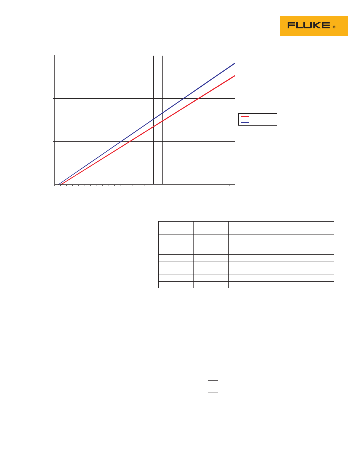
Figure 1. RTD Curves.
Equation 2: Rt = R0 [1 + At + Bt2 + C(t — 100)t3]
Figure 1 shows the difference between temperature values produced by the linear equation and
the polynomial between 200 and 500 °C. Note that
at 240 ohms, the polynomial curve of Equation 2
gives a more accurate temperature 16 °C higher
than the linear equation.
The Fluke 726 uses the polynomial in Equation
2 and it has built-in constants to support most
common RTD’s. Standard RTD’s supported by the
Fluke 726 are shown in Table 1.
Older or specialized equipment may use nonstandard RTDs. Well-equipped standards labs can
improve the accuracy of an RTD by adjusting the
constants to suit a particular sensor. The Fluke 726
allows you to check less common RTD’s or take
advantage of RTD’s that have been characterized,
by specifying your own values for R
For example, for the common Pt 385 RTD with
, A, B and C.
0
100 W resistance at 0 °C, the constants are:
R
= 100 W
0
A = 3.9083 x 10
B = -5.775 x 10
C = -4.183 x 10
Note: Instruments installed before and up to the early 1990s used a
slightly different temperature scale (IPTS-68) than newer instruments
(ITS-90). When a calibrator using ITS-90 RTD curves is used to
calibrate an instrument using IPTS-68 errors will result. The errors
are extremely small at room temperature and increase to a maximum
of 0.36 °C at 760 °C.
-3
-7
-12
RTD Type Reference R0, Metal a Range
Ohms W/W/°C °C
Pt 100 (3916) 100 Platinum 0.003916 -200 to 630
Pt 100 (385)* 100 Platinum 0.00385 -200 to 800
Pt 200 (385) 200 Platinum 0.00385 -200 to 630
Pt 500 (385) 500 Platinum 0.00385 -200 to 630
Pt 1000 (385) 1000 Platinum 0.00385 -200 to 630
Pt 100 (3926) 100 Platinum 0.003926 -200 to 630
Ni 120 (672) 120 Nickel 0.00672 -80 to 260
Cu 10 (42) 10 Copper 0.0042 -10 to 250
Table 1: Standard RTDs types included in the Fluke 726.
Pt 100 (385) is the IEC and ASTM standard.
Another common form of Equation 2, the Call-
endar Van Dusen or CVD, uses the constants a, d,
and b. This alternative form is directly derived from
Equation 1 and uses the same constant a. And even
though the two polynomials produce the same
results, the constants are different. The Fluke 726
uses the constants A, B, and C. If you know the a,
d, and b constants for an RTD you can convert them
to A, B, C constants by using Equations 3, 4 and 5.
Equation 3: A = a +
Equation 4: B = —
Equation 5: C = —
a.d
100
a.d
100
a.b
100
2
4
2 Fluke Corporation Measuring uncommon RTDs with the Fluke 726
Page 3
Loading custom RTD constants into the Fluke 726
Setting up communications
Figure 2.
The Fluke 700SC Serial Interface Cable (PN
667425) is used to communicate with the Fluke
726. The serial cable connects to the round multipin connector at the top of the 726 and to a 9-pin
serial port on your PC. The serial cable can only
interface with one instrument or module at a time.
After connecting the cable, make sure the 726
is turned on. Call up the Windows HyperTerminal
Program. It is usually listed in the Windows Start
Programs menu under Accessories, Communications. The HyperTerminal program will ask you
to set up a file name to store your communication
settings. You can select any icon and click OK to
continue.
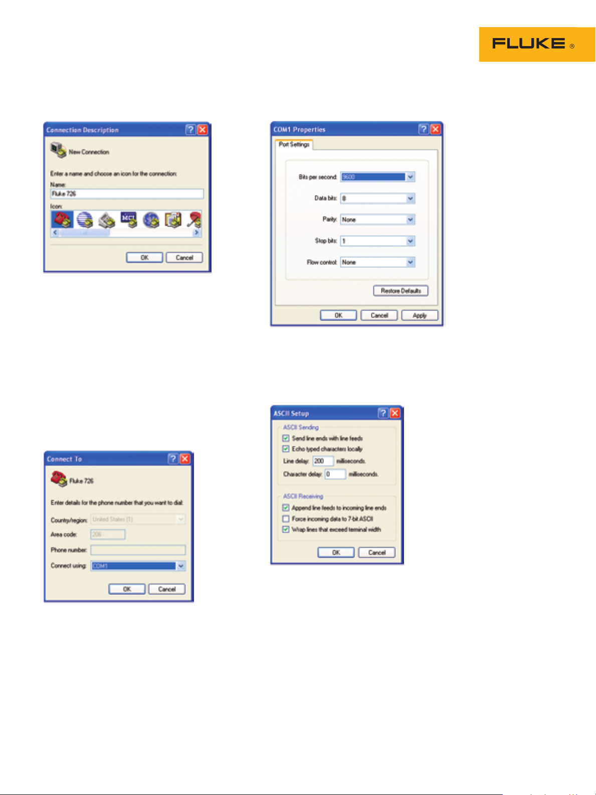
Figure 4.
Next, a COM Properties box will come up. Set
baud rate (9600 in Figure 4), data bits, parity,
stop bits and flow control as shown in the Figure
4. Once your settings match Figure 4, click OK to
continue.
Figure 3.
A second dialog box, “Connect To”, will pop up.
Skip down to the bottom, where it says “Connect
Using:” Select the COM port you connected to
the 726.
3 Fluke Corporation Measuring uncommon RTDs with the Fluke 726
Figure 5.
To make it easier to read the commands and
responses, you can make some adjustments to the
way the HyperTerminal program treats screen text.
Under the File menu select Properties and click on
the Settings tab. Click on the button labeled ASCII
Setup. You will see a dialog like the one shown in
Figure 5. Match the settings shown in the figure.
Note that adding the 200 ms line delay makes it
possible to send short scripts to the 726. More on
this later.
To test the connection, type:
*idn?
After you hit Enter, the 726 should respond with
“FLUKE,726,0,X.X” where X.X is the version of the
firmware in the instrument.
Page 4
Sending custom RTD constants to the
Fluke 726
Once communication is established you can load
custom constants into the 726. You can also send
queries to the 726 to check the current settings and
to verify your changes. Here is an overview of the
steps to modify the constants:
1. Set the RTD type to the one of the custom types
(CUST1, CUST2 or CUST3)
2. Set the minimum and maximum temperatures for
the custom RTD
3. Set the constants R0, A, B, and C
4. Assign a six-character name that will appear
on the front panel of the instrument to help the
operator choose RTD types
The best way to show the detailed process is
through an example. Let’s say we need to measure
an RTD with the following attributes:
Range is from 0 to 630 °C
R
= 100 W
0
A = 3.9692 x 10
B = -5.8495 x 10
-3
-7
C = unknown and unnecessary since range is
0 °C or greater
Rather than having to type all of the commands
each time we want to change the constants, we
can define short text files and send them using
the HyperTerminal program. The Windows Notepad program may be used to create and edit the
command scripts.
The text file in Figure 6 is designed to query all
of the parameters associated with the RTD type
CUST1. Try building and sending this query file first.
It is a good practice script and is useful for verifying
any changes you make to the constants later.
When you finish editing the script file, make sure
you hit Enter after the last command (in this example “cust1_alias?”). The cursor should be blinking
below the last command when you save the file.
This will ensure that the 726 sees the endline after
the last command and processes it.
To send a script file to the 726, click on Transfer,
Send Text File in HyperTerminal. The 726 will
respond to each of the queries with the current
values of each constant.
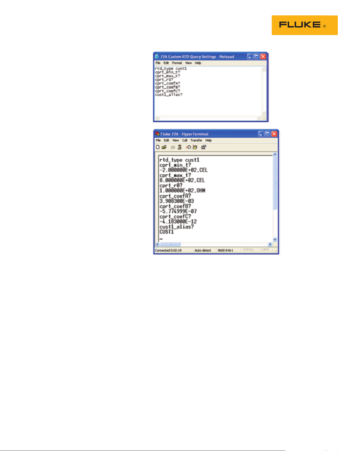
Figure 6. A script used to query custom RTD settings and the results
of sending it to the 726. Each query command is followed by a
response from the 726.
The HyperTerminal window shown in Figure
6 shows the response of the 726 to sending the
query commands. Each command that ends in a
question mark is followed by a response from the
726. These response are the factory default values
for the CUST1 RTD.
4 Fluke Corporation Measuring uncommon RTDs with the Fluke 726
Page 5
Note: The cursor should be
here before you save the file.
Using custom-defined RTD’s with the
Fluke 726
To use a custom RTD with the Fluke 726 you simply
select it by pressing the RTD button on the front
panel. This will cycle you through all of the available RTD types, including the three custom ones.
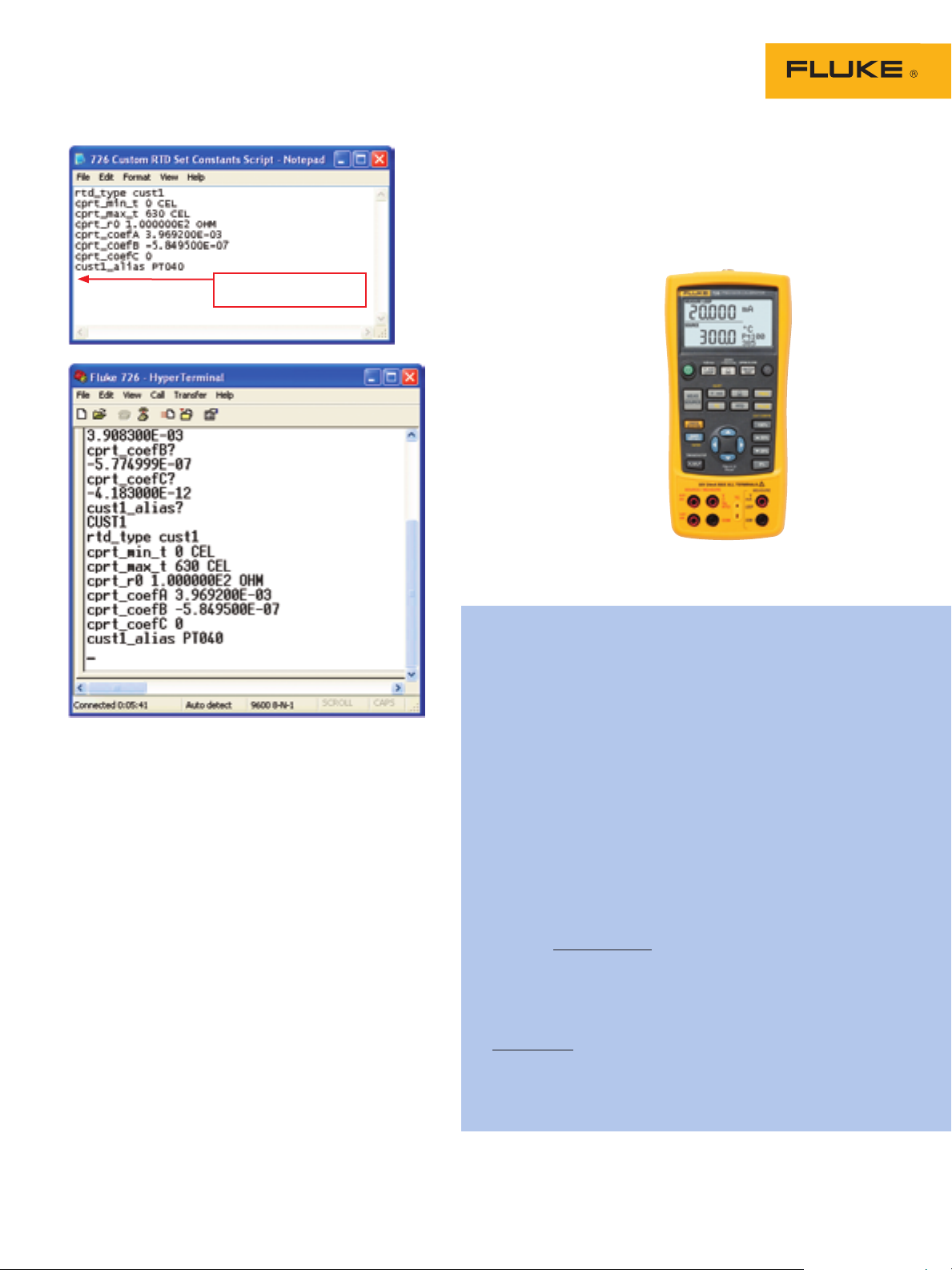
Figure 7. A script used to define custom RTD constants and the
results of sending it to the 726.
Figure 7 shows a script to change the constants
for the CUST1 type RTD. The script can be developed in Windows Notepad, just like the previous
example. Here’s how it works:
The script activates the RTD measurement and
•
sets the RTD type to CUST1.
It sends commands to establish new min and
•
max limits for the new RTD type.
The next three commands set the A, B, and C
•
constants. In this example we are limiting the
sensor to temperatures of 0 °C or greater, and
setting the C coefficient to 0.
The alias command will name the new RTD
•
PT040.
Note that numbers may be in integer, decimal or scientific notation.
Once the file is prepared, click on Transfer, Send
Text File in HyperTerminal to send the file to the
726. You can verify that the 726 has the correct
constants by using the query script from Figure 6.
Your 726 is now ready to make measurements
using your custom RTD curve.
Calculating the combined uncertainty of any
meter and transducer
The combination of the Fluke 726 and an RTD will have an
uncertainty that considers both the meter and the transducer.
Since the uncertainties of the meter and probe are independent of each other, rather than simply adding the uncertainties, we can take the square root of the sum of the squares.
The uncertainty of the Fluke 726 is expressed as a percentage of reading with a noise floor that is determined by the
range. The temperature specifications are 0.15 °C uncertainty
for the meter, 0.1 °C uncertainty for the probe. Here’s an
example of how to calculate the uncertainty for the Fluke 726
in °C at 100 °C.
Once you have the uncertainties of both the meter and the
probe at a particular point, you can combine these uncertainties to come up with the uncertainty of the system. The
formula for combining these independent uncertainties is:
= √U
2
probe
U
system
For example, the uncertainty of the Fluke 726 at 100 °C is
0.15 °C as calculated above. If we have an RTD whose uncertainty at 100 °C is 0.1 °C, then the combined accuracy will be
plus or minus
2
√0.1
+ 0.152 = 0.18 °C
*The above equation assumes that the U values follow a normal distribution. A
metrology standpoint would recommend dividing the ‘U’ values by √3 and then
doing the root sum square, when using the manufacture’s specification.
+ U
2
meter
*
5 Fluke Corporation Measuring uncommon RTDs with the Fluke 726
Page 6

726 Serial Command List
Command Response/Actions Command Arguments Comment Ch 1 Ch 2
*IDN? Returns the ID string “FLUKE,726,0, Verify model
{sw_rev}” where sw_rev is the number, serial
firmware revision number and
firmware rev.
FUNC? Returns {Upper},{Lower} Answers with
{Upper} responses (Channel 1) the configured
DCI, DCI_LOOP, DCV, DCI_ERROR, function for the
DCI_ERROR_LOOP upper and lower
{Lower} responses display.
DCI, DCMV, DCV, DCI_SIM, TC, RTD,
FREQUENCY, PULSE_TRAIN
VAL? Returns the measured value with base
units for the upper and lower display
{upper_val},{upper_units},{lower_val},
{lower _units},
upper_units: V, A, PERCENT
lower _units: V, CEL, FAR, A, OHM,
CPM, HZ, COUNT
UPPER_MEAS 1 argument, valid settings: DCI, Set upper
DCI_LOOP, DCV, DCI_ERROR, channel
DCI_ERROR_LOOP measure mode.
OUT Arguments: {value} {units} Configures the
Multipliers u for micro, m for milli, and output source
k for kilo are accepted. function. If the
units: {value} and {units}
-V used for mV and Volts, the V_range are valid, this
command can be used to switch ranges command will
-CEL used for RTD, TC AND TC mV change modes if
-FAR used for RTD and TC necessary and set
-A used for mA (see SIM for mA SIM) the output value
-OHM used for RTD ohms, RTD_TYPE to {value} and
must be set to ohms {units} in that
-CPM used for frequency mode.
-HZ used for HZ and KHZ frequency
(unit will auto range)
-COUNT used for pulse
OUT? Returns the output (source) value Verify the output
with units or none. function and units.
FREQ_UNIT 1 argument: CPM, HZ or KHZ Set the output
frequency range.
FREQ_UNIT? Returns CPM, HZ, KHZ Verify the
frequency range.
LOWER_MEAS 1 argument, Valid Modes: Configures the
DCI, DCMV, DCV, TC, RTD, measurement
FREQUENCY, PULSE_TRAIN function. Sets the
specified measure
mode.
SIM 1 Argument {value} Multipliers u for If the value is
micro, m for milli, and k for kilo are valid, this
accepted,. A is for amps command will
change modes if
necessary and set
the output value
to {value} in that
mode.
SIM? Returns the simulate value in Amps Verify the SIM
with units or none output.
V_RANGE 1 Argument VOLTS or MVOLTS Sets the voltage
range.
V_RANGE? Returns the voltage range VOLTS or Verify the voltage
MVOLTS range.
PULSE_FREQ 2 arguments {number}{units}. Sets the pulse
(units CPM ,Hz ,Khz) output frequency
and range.
PULSE_FREQ? Returns the pulse output frequency Verify the pulse
with units. frequency.
• •
• •
• •
•
•
•
•
•
•
•
•
•
•
continued on next page
6 Fluke Corporation Measuring uncommon RTDs with the Fluke 726
Page 7

726 Serial Command List cont.
Command Response/Actions Command Arguments Comment Ch 1 Ch 2
FREQ_LEVEL 1 Argument, valid values: 1-20 V Sets the pulse
output and
frequency output
voltage.
FREQ_LEVEL? Returns the pulse output and Verify the
frequency output voltage 1-20 V frequency voltage
level.
TRIG Toggles the pulse mode and totalize Initialize totalized
trigger for read and source. pulse
measurement
or output.
TRIG? Returns the state of the pulse mode Verify TRIG state.
trigger, TRIGGERED, UNTRIGGERED
or NONE.
TC_TYPE One argument, valid settings: B, C, E, Set TC type.
J, K, L, N, R, S, T, U, BP, XK, MV
TC_TYPE? Returns TC type Verify TC type.
B, C, E, J, K, L, N, R, S, T, U, BP, XK, MV
TSENS_TYPE 1 argument TC or RTD Sets the sensor
type TC or RTD.
TSENS_TYPE? Returns the sensor type TC or RTD Verify is set for
RTD or TC.
CJC_STATE One argument ON or OFF Thermocouple
cold junction
compensation.
CJC_STATE? Returns ON or OFF Verify CJC state.
RTD_TYPE 1 argument: NI120, PT392_100, Sets RTD type
PT385_100, PTJIS_100, PT385_200,
PT385_500, PT385_1000, CU_10,
CUST1, CUST2, CUST3, OHMS
RTD_TYPE? Returns RTD type Verify the RTD
NI120, PT392_100, PT385_100, type setting.
PTJIS_100, PT385_200, PT385_500,
PT385_1000, CU_10, CUST1, CUST2,
CUST3, OHMS
CPRT_R0 2 arguments {number} OHM. RTD_TYPE must
Sets the custom CPRT R0. be either CUST1,
CUST2 or CUST3.
CPRT_R0? Returns CPRT R0 with units OHM.
CPRT_MIN_T 2 arguments {number} CEL.
CPRT_MIN_T? Returns {number} CEL.
CPRT_MAX_T 2 arguments {number} CEL.
CPRT_MAX_T? Returns {number} CEL.
CPRT_COEFA 1 argument. Sets the custom CPRT
Coefficient A.
CPRT_COEFA? Returns the custom CPRT Coefficient A.
CPRT_COEFB 1 argument. Sets the custom CPRT
Coefficient B.
CPRT_COEFB? Returns the custom CPRT Coefficient B.
CPRT_COEFC 1 argument. Sets the custom CPRT
Coefficient C.
CPRT_COEFC? Returns the custom CPRT Coefficient C.
RTD_WIRE 1 argument, 2W, 3W or 4W.
Sets RTD read wire.
RTD_WIRE? Returns RTD read wire. Verify connection
setting.
TEMP_UNIT 1 argument. Sets temperature units, CEL: Celsius
CEL or FAR FAR: Fahrenheit
TEMP_UNIT? Returns temperature units, CEL or FAR
continued on next page
•
•
•
•
•
•
•
•
•
•
•
•
•
•
•
•
•
•
•
•
•
•
•
•
•
•
•
7 Fluke Corporation Measuring uncommon RTDs with the Fluke 726
Page 8

726 Serial Command List
Command Response/Actions Command Arguments Comment Ch 1 Ch 2
CUST1_ALIAS 1 argument, sets screen name for
CUST1 RTD.
CUST1_ALIAS? Returns screen name for CUST1 RTD Verify RTD 1 alias.
CUST2_ALIAS 1 argument, sets screen name for
CUST2 RTD.
CUST2_ALIAS? Returns screen name for CUST2 RTD. Verify RTD 2 alias.
•
•
•
•
CUST3_ALIAS1 1 argument, sets screen name for
CUST3 RTD.
CUST3_ALIAS? Returns screen name for CUST3 RTD. Verify RTD 3 alias
HART_ON Turns HART mode on. Switches in 250
ohm resistor.
HART_OFF Turns HART mode off. Switches out 250
ohm resistor.
HART? Returns state of hart mode, ON or OFF
*CLS Clear the error queue
FA U LT Returns error code FILO
ERROR CODES: NONNUMERIC_ENRTY (100)
EBUFFER_OVERFLOW (101)
INVALID_UNITS_CODE (102)
ENTRY_OVER_RNG (103)
ENTRY_UNDER_RNG (104)
MISSING_PARM (105)
INVALID_UNIT_PARM (106)
INVALID_SENSOR_TYPE (108)
UNKNOWN_COMMAND (110)
BAD_PARM_VALUE (111)
INPUT_BUFF_OVERFLOW (112)
MSG_BUFF_OVERFLOW (113)
OUTPUT_BUFF_OVERFLOW (114)
OUTPUT_OVERLOAD (115)
CAL_START Initiates a password protected See Cal. Manual
calibration (password = 627) for details
•
•
• •
• •
• •
•
•
•
•
•
•
•
•
8 Fluke Corporation Measuring uncommon RTDs with the Fluke 726
Fluke. Keeping your world
up and running.
Fluke Corporation
PO Box 9090, Everett, WA USA 98206
Fluke Europe B.V.
PO Box 1186, 5602 BD
Eindhoven, The Netherlands
For more information call:
In the U.S.A. (800) 443-5853 or
Fax (425) 446-5116
In Europe/M-East/Africa +31 (0) 40 2675 200 or
Fax +31 (0) 40 2675 222
In Canada (800)-36-FLUKE or
Fax (905) 890-6866
From other countries +1 (425) 446-5500 or
Fax +1 (425) 446-5116
Web access: http://www.fluke.com
©2007 Fluke Corporation. All rights reserved.
Specifications subject to change without notice.
Printed in U.S.A. 6/2007 2546483 A-EN-N Rev B
®
 Loading...