Emerson Fisher Vee-Ball V150E Reference Manual

CONTROL VALVE

SOURCEBOOK

PULP & PAPER

Copyright © 2011 Fisher Controls International LLC
All Rights Reserved.

Fisher, ENVIRO-SEAL, Whisper Trim, Cavitrol, WhisperFlo, Vee‐Ball, Control‐Disk, NotchFlo, easy‐e and FIELDVUE are marks
owned by Fisher Controls International LLC, a business of Emerson Process Management. The Emerson logo is a trademark and
service mark of Emerson Electric Co. All other marks are the property of their respective owners.

This publication may not be reproduced, stored in a retrieval system, or transmitted in whole or in part, in any form or by any means,
electronic, mechanical, photocopying, recording or otherwise, without the written permission of Fisher Controls International LLC.

Printed in U.S.A., First Edition

Table of Contents

Introduction v

Chapter 1 Control Valve Selection 1-1

Chapter 2 Actuator Selection 2-1

Chapter 3 Liquid Valve Sizing 3-1

Chapter 4 Cavitation & Flashing 4-1

Chapter 5 Gas Valve Sizing 5-1

Chapter 6 Control Valve Noise 6-1

Chapter 7 Steam Conditioning 7-1

Chapter 8 Process Overview 8-1

Chapter 9 Pulping 9-1

Chapter 10A Batch Digesters 10A-1

Chapter 10B Continuous Digesters 10B-1

Chapter 11 Black Liquor Evaporators/Concentrators 11-1

Chapter 12 Kraft Recovery Boiler 12-1

Chapter 13 Recausticizing & Lime Recovery 13-1

Chapter 14 Bleaching & Brightening 14-1

Chapter 15 Stock Preparation 15-1

Chapter 16 Wet End Chemistry 16-1

Chapter 17 Paper Machine 17-1

Chapter 18 Power & Recovery Boiler 18-1

iii

iv

Pulp and Paper Control Valves

Introduction

This sourcebook’s intent is to introduce a pulp
and paper mill’s processes, as well as the use of
control valves in many of the processes found in
the mill. It is intended to help you:

D Understand pulp and paper processes
D Learn where control valves are typically

located within each process

D Identify valves commonly used for specific

applications

D Identify troublesome/problem valves within

the process
The information provided will follow a standard

format of:

D Description of the process
D Functional drawing of the process
D FisherR valves to be considered in each

process and their associated function

Control Valves

Valves described within a chapter are labeled
and numbered corresponding to the identification
used in the proces s flow chart for that chapter.
Their valve function is described, and a
specification section gives added information on
process conditions, names of Fisher valves that
may be considered, process impact of the valve,
and any special considerations for the process
and valve(s) of choice.

Process Drawings

The process drawings within each chapter show
major equipment items, their typical placement
within the processing system, and process flow
direction. Utilities and pumps are not shown
unless otherwise stated.

Many original equipment manufacturers (OEMs)
provide equipment to the pulp and paper
industry, each with their own processes and
proprietary information. Process drawings are
based on general equipment configurations
unless otherwise stated.

D Impacts and/or considerations for

troublesome/problem valves

Valve Selection

The information presented in this sourcebook is
intended to assist in understanding the control
valve requirements of general pulp and paper
mill’s processes.

Since every mill is different in technology and
layout, the control valve requirements and
recommendations presented by this sourcebook
should be considered as general guidelines.
Under no circumstances should this information
alone be used to select a control valve without
ensuring the proper valve construction is identified
for the application and process conditions.

All valve considerations should be reviewed by the
local business representative as part of any valve
selection or specification activity.

Problem Valves

Often there are references to valve-caused
problems or difficulties. The list of problems
include valve erosion from process media,
stickiness caused by excessive friction (stiction),
excessive play in valve to actuator linkages
(typically found in rotary valves) that causes
deadband, excessive valve stem packing
leakage, and valve materials that are
incompatible with the flowing medium. Any one,
or a combination of these difficulties, may affect
process quality and throughput with a resulting
negative impact on mill profitability.

Many of these problems can be avoided or
minimized through proper valve selection.
Consideration should be given to valve style and
size, actuator capabilities, analog versus digital
instrumentation, materials of construction, etc.
Although not being all-inclusive, the information
found in this sourcebook should facilitate the
valve selection process.

v

vi

Chapter 1

Control Valve Selection

In the past, a customer simply requested a control
valve and the manufacturer offered the product
best-suited for the job. The choices among the
manufacturers were always dependent upon
obvious matters such as cost, delivery, vendor
relationships, and user preference. However,
accurate control valve selection can be
considerably more complex, especially for
engineers with limited experience or those who
have not kept up with changes in the control valve
industry.

An assortment of sliding-stem and rotary valve
styles are available for many applications. Some
are touted as “universal” valves for almost any
size and service, while others are claimed to be
optimum solutions for narrowly defined needs.
Even the most knowledgeable user may wonder
whether they are really getting the most for their
money in the control valves they have specified.

Like most decisions, selection of a control valve
involves a great number of variables; the everyday
selection process tends to overlook a number of
these important variables. The following
discussion includes categorization of available
valve types and a set of criteria to be considered in
the selection process.

What Is A Control Valve?

Process plants consist of hundreds, or even
thousands, of control loops all networked together
to produce a product to be offered for sale. Each
of these control loops is designed to control a
critical process variable such as pressure, flow,
level, temperature, etc., within a required operating
range to ensure the quality of the end-product.

These loops receive, and internally create,
disturbances that detrimentally affect the process
variable. Interaction from other loops in the
network provides disturbances that influence the
process variable. To reduce the effect of these
load disturbances, sensors and transmitters collect
information regarding the process variable and its
relationship to a desired set point. A controller then
processes this information and decides what must
occur in order to get the process variable back to
where it should be after a load disturbance occurs.
When all measuring, comparing, and calculating
are complete, the strategy selected by the
controller is implemented via some type of final
control element. The most common final control
element in the process control industries is the
control valve.

A control valve manipulates a flowing fluid such as
gas, steam, water, or chemical compounds to
compensate for the load disturbance and keep the
regulated process variable as close as possible to
the desired set point.

Many people who speak of “control valves” are
actually referring to “control valve assemblies.”
The control valve assembly typically consists of
the valve body, the internal trim parts, an actuator
to provide the motive power to operate the valve,
and a variety of additional valve accessories,
which may include positioners, transducers, supply
pressure regulators, manual operators, snubbers,
or limit switches.

It is best to think of a control loop as an
instrumentation chain. Like any other chain, the
entire chain is only as good as its weakest link. It
is important to ensure that the control valve is not
the weakest link.

www.Fisher.com

Valve Types and Characteristics

The control valve regulates the rate of fluid flow as
the position of the valve plug or disk is changed by
force from the actuator. To do this, the valve must:

D Contain the fluid without external leakage.
D Have adequate capacity for the intended

service.

D Be capable of withstanding the erosive,
corrosive, and temperature influences of the
process.

D Incorporate appropriate end connections to
mate with adjacent pipelines and actuator
attachment means to permit transmission of
actuator thrust to the valve plug stem or rotary
shaft.

Many styles of control valve bodies have been
developed. Some can be used effectively in a
number of applications while others meet specific
service demands or conditions and are used less
frequently. The subsequent text describes popular
control valve body styles utilized today.

Globe Valves

Single-Port Valve Bodies

Single-port is the most common valve body style
and is simple in construction. Single-port valves
are available in various forms, such as globe,
angle, bar stock, forged, and split constructions.
Generally, single-port valves are specified for
applications with stringent shutoff requirements.
They use metal-to-metal seating surfaces or
soft-seating with PTFE or other composition
materials forming the seal.

W7027-1

Figure 1-1. Single-Ported Globe-Style Valve

Body

characteristics. Retainer-style trim also offers ease
of maintenance with flow characteristics altered by
changing the plug. Cage or retainer-style
single-seated valve bodies can also be easily
modified by a change of trim parts to provide
reduced-capacity flow, noise attenuation, or
cavitation eliminating or reducing trim (see
chapter 4).

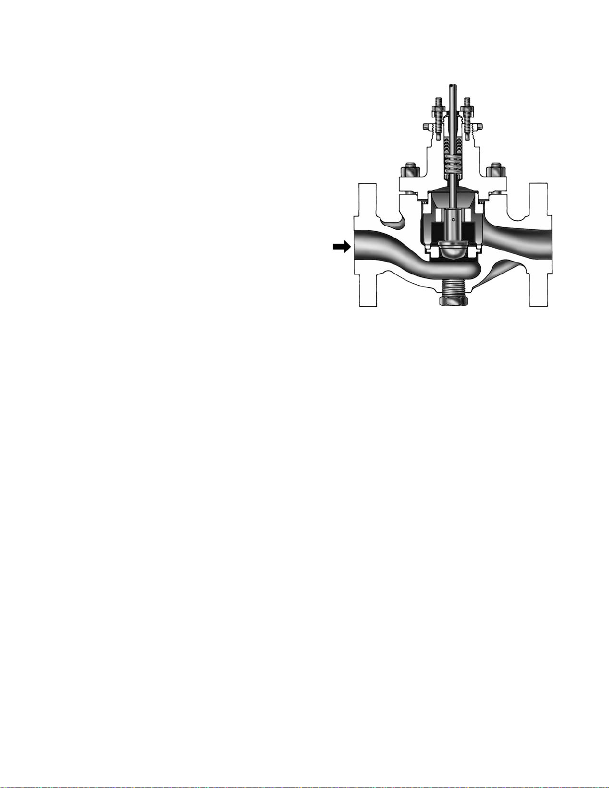
Figure 1-1 shows one of the more popular styles of
single-ported or single-seated globe valve bodies.
They are widely used in process control
applications, particularly in sizes NPS 1 through
NPS 4. Normal flow direction is most often flow-up
through the seat ring.

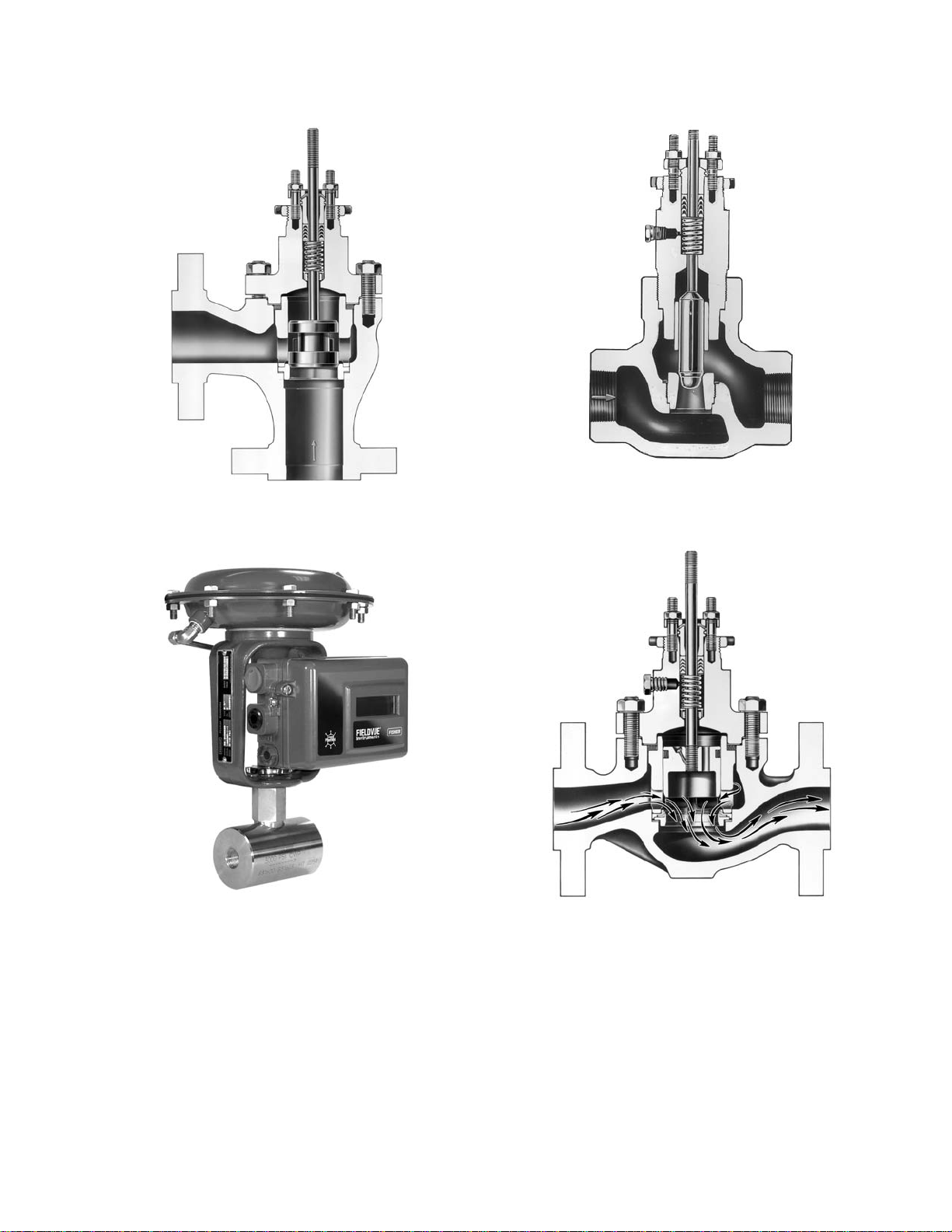
Angle valves are nearly always single ported, as
shown in figure 1-2. This valve has cage-style trim
construction. Others might have screwed-in seat
rings, expanded outlet connections, restricted trim,
and outlet liners for reduction of erosion damage.

Single-port valves can handle most service
requirements. Because high pressure fluid is
normally loading the entire area of the port, the
unbalance force created must be considered when
selecting actuators for single-port control valve
bodies. Although most popular in the smaller
sizes, single-port valves can often be used in NPS
4 to 8 with high thrust actuators.

Many modern single-seated valve bodies use cage
or retainer-style construction to retain the seat ring
cage, provide valve plug guiding, and provide a
means for establishing particular valve flow

1−2

Bar stock valve bodies are often specified for
corrosive applications in the chemical industry
(figure 1-3), but may also be requested in other
low flow corrosive applications. They can be
machined from any metallic bar-stock material and
from some plastics. When exotic metal alloys are
required for corrosion resistance, a bar-stock valve
body is normally less expensive than a valve body
produced from a casting.

High pressure single-ported globe valves are often
found in power plants due to high pressure steam
(figure 1-4). Variations available include

W0971

Figure 1-2. Flanged Angle-Style

Control Valve Body

W0540

Figure 1-4. High Pressure Globe-Style

Control Valve Body

W9756

Figure 1-3. Bar Stock Valve Body

cage-guided trim, bolted body-to-bonnet
connection, and others. Flanged versions are
available with ratings to Class 2500.

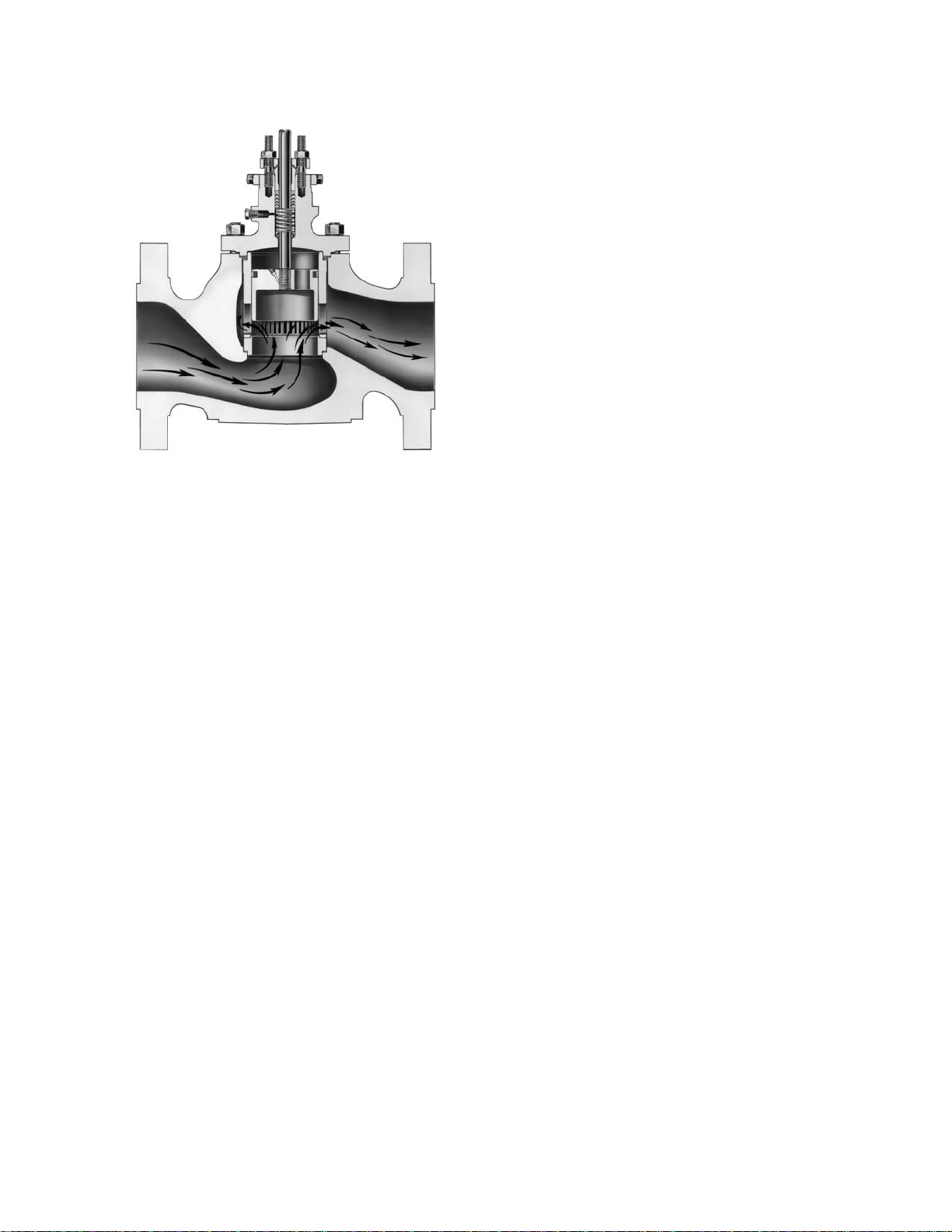
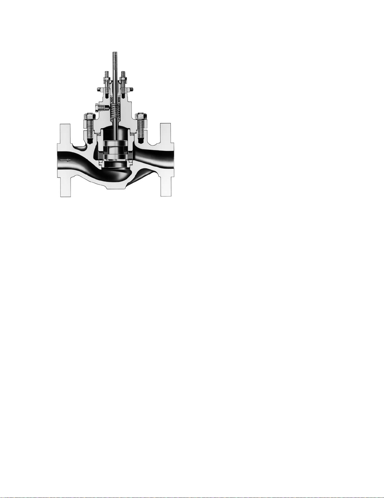
Balanced-Plug Cage-Style Valve
Bodies

This popular valve body style, single-ported in the
sense that only one seat ring is used, provides the
advantages of a balanced valve plug often

W0992-4

Figure 1-5. Valve Body with Cage-Style Trim,

Balanced Valve Plug, and Soft Seat

associated only with double-ported valve bodies
(figure 1-5). Cage-style trim provides valve plug
guiding, seat ring retention, and flow
characterization. In addition, a sliding piston
ring-type seal between the upper portion of the
valve plug and the wall of the cage cylinder
virtually eliminates leakage of the upstream high
pressure fluid into the lower pressure downstream
system.

1−3

W0997

Figure 1-6. High Capacity Valve Body with

Cage-Style Noise Abatement Trim

liquid service. The flow direction depends upon the
intended service and trim selection, with
unbalanced constructions normally flow-up and
balanced constructions normally flow-down.

Port-Guided Single-Port Valve Bodies

D Usually limited to 150 psi (10 bar) maximum

pressure drop.

D Susceptible to velocity-induced vibration.
D Typically provided with screwed in seat rings

which might be difficult to remove after use.

Three-Way Valve Bodies

D Provide general converging (flow-mixing) or

diverging (flow-splitting) service.

D Best designs use cage-style trim for positive

valve plug guiding and ease of maintenance.

Downstream pressure acts upon both the top and
bottom sides of the valve plug, thereby nullifying
most of the static unbalance force. Reduced
unbalance permits operation of the valve with
smaller actuators than those necessary for
conventional single-ported valve bodies.

Interchangeability of trim permits the choice of
several flow characteristics or of noise attenuation
or anticavitation components. For most available
trim designs, the standard direction of flow is in
through the cage openings and down through the
seat ring. These are available in various material
combinations, sizes through NPS 20, and pressure
ratings to Class 2500.

High Capacity, Cage-Guided Valve
Bodies

This adaptation of the cage-guided bodies
mentioned above was designed for noise
applications, such as high pressure power plants,
where sonic steam velocities are often
encountered at the outlet of conventional valve
bodies (figure 1-6).

The design incorporates oversized end
connections with a streamlined flow path and the
ease of trim maintenance inherent with cage-style
constructions. Use of noise abatement trim
reduces overall noise levels by as much as 35
decibels. The design is also available in cageless
versions with a bolted seat ring, end connection
sizes through NPS 20, Class 600, and versions for

D Variations include trim materials selected for
high temperature service. Standard end
connections (flanged, screwed, butt weld, etc.) can
be specified to mate with most any piping scheme.

D Actuator selection demands careful
consideration, particularly for constructions with
unbalanced valve plug.

A balanced valve plug style three-way valve body
is shown with the cylindrical valve plug in the down
position (figure 1-7). This position opens the
bottom common port to the right-hand port and
shuts off the left-hand port. The construction can
be used for throttling mid-travel position control of
either converging or diverging fluids.

Rotary Valves

Traditional Butterfly Valve

Standard butterfly valves are available in sizes
through NPS 72 for miscellaneous control valve
applications. Smaller sizes can use versions of
traditional diaphragm or piston pneumatic
actuators, including the modern rotary actuator
styles. Larger sizes might require high output
electric or long-stroke pneumatic cylinder
actuators.

Butterfly valves exhibit an approximately equal
percentage flow characteristic. They can be used

1−4

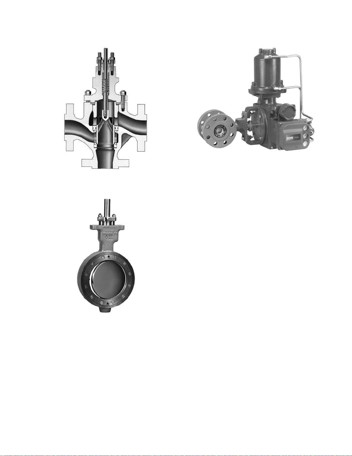
W8380

W9045-1

Figure 1-7. Three Way Valve with

Balanced Valve Plug

W4641

Figure 1-8. High-Performance Butterfly

Control Valve

for throttling service or for on-off control. Soft-seat
constructions can be obtained by utilizing a liner or
by including an adjustable soft ring in the body or
on the face of the disk.

Figure 1-9. Eccentric-Disk Rotary-Shaft

Control Valve

D Offer an economic advantage, particularly in
larger sizes and in terms of flow capacity per dollar
investment.

D Mate with standard raised-face pipeline
flanges.

D Depending on size, might require high output
or oversized actuators due to valve size valves or
large operating torques from large pressure drops.

D Standard liner can provide precise shutoff
and quality corrosion protection with nitrile or
PTFE liner.

Eccentric-Disk Control Valve

Eccentric disk rotary control valves are intended
for general service applications not requiring
precision throttling control. They are frequently
applied in applications requiring large sizes and
high temperatures due to their lower cost relative
to other styles of control valves. The control range
for this style of valve is approximately one third as
large as a ball or globe-style valves.
Consequently, additional care is required in sizing
and applying this style of valve to eliminate control
problems associated with process load changes.
They are well-suited for constant process load
applications.

D Provide effective throttling control.

D Require minimum space for installation

(figure 1-8).

D Provide high capacity with low pressure loss

through the valves.

D Linear flow characteristic through 90 degrees
of disk rotation (figure 1-9).

D Eccentric mounting of disk pulls it away from
the seal after it begins to open, minimizing seal
wear.

1−5

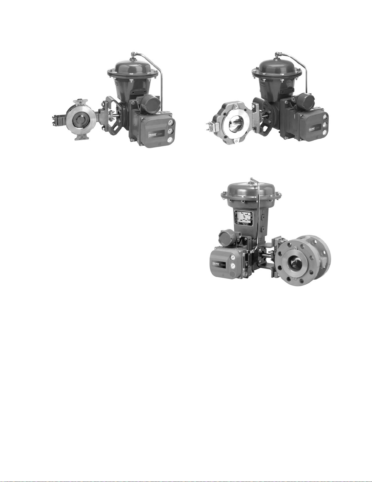
W9425 W9418

WAFER STYLE SINGLE FLANGE STYLE

Figure 1-10. Fisher Control-Disk Valve with 2052 Actuator and FIELDVUE DVC6200 Digital Valve Controller

D Bodies are available in sizes through NPS 24

compatible with standard ASME flanges.

D Utilize standard pneumatic diaphragm or

piston rotary actuators.

D Standard flow direction is dependent upon
seal design; reverse flow results in reduced
capacity.

Control-Disk Valve

The Control-Diskt valve (figure 1-10) offers
excellent throttling performance, while maintaining
the size (face-to-face) of a traditional butterfly
valve. The Control-Disk valve is first in class in
controllability, rangeability, and tight shutoff, and it
is designed to meet worldwide standards.

D Utilizes a contoured edge and unique
patented disk to provide an improved control range
of 15 - 70% of valve travel. Traditional butterfly

lever design to increase torque range within each
actuator size.

valves are typically limited to 25% - 50% control
range.

V-notch Ball Control Valve

D Includes a tested valve sealing design,
available in both metal and soft seats, to provide
an unmatched cycle life while still maintaining
excellent shutoff

D Spring loaded shaft positions disk against the
inboard bearing nearest the actuator allowing for
the disk to close in the same position in the seal,
and allows for either horizontal or vertical
mounting.

D Complimenting actuator comes in three,
compact sizes, has nested springs and a patented

This construction is similar to a conventional ball
valve, but with patented, contoured V-notch in the
ball (figure 1-11). The V-notch produces an
equal-percentage flow characteristic. These
control valves provide precise rangeability, control,
and tight shutoff.

pressure drop.

erosive or viscous fluids, paper stock, or other
slurries containing entrained solids or fibers.

W8172-2

Figure 1-11. Rotary-Shaft Control Valve

with V-Notch Ball

D Straight-through flow design produces little

D Bodies are suited to provide control of

1−6

on-off operation. The flanged or flangeless valves
feature streamlined flow passages and rugged
metal-trim components for dependable service in
slurry applications.

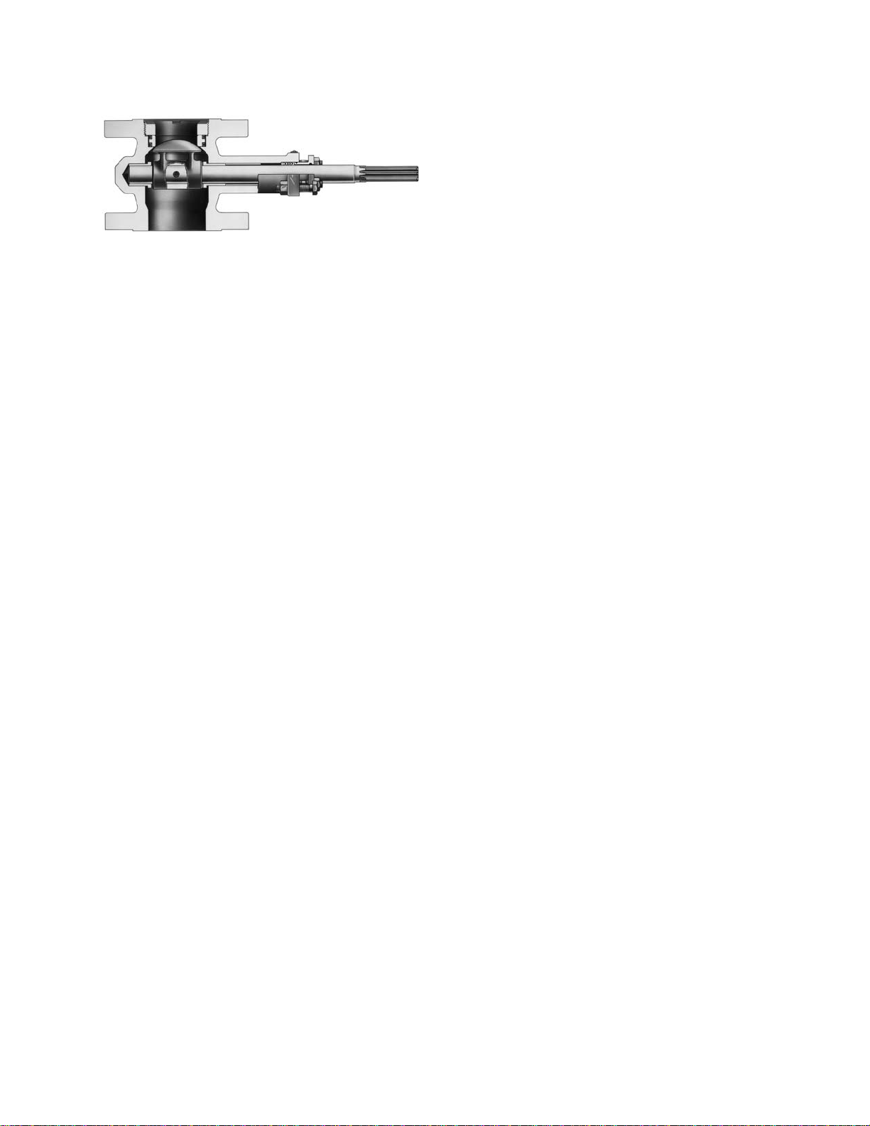
W4170-4

Figure 1-12. Sectional of Eccentric-Plug

Control Valve Body

D They utilize standard diaphragm or piston
rotary actuators.

D Ball remains in contact with seal during
rotation, which produces a shearing effect as the
ball closes and minimizes clogging.

D Bodies are available with either heavy-duty or
PTFE-filled composition ball seal ring to provide
excellent rangeability in excess of 300:1.

D Bodies are available in flangeless or
flanged-body end connections. Both flanged and
flangeless valves mate with Class 150, 300, or 600
flanges or DIN flanges.

D Valves are capable of energy absorbing
special attenuating trim to provide improved
performance for demanding applications.

Eccentric-Plug Control Valve

Control Valve End Connections

The three common methods of installing control
valves in pipelines are by means of:

D Screwed pipe threads
D Bolted gasketed flanges
D Welded end connections

Screwed Pipe Threads

Screwed end connections, popular in small control
valves, are typically more economical than flanged
ends. The threads usually specified are tapered
female National Pipe Thread (NPT) on the valve
body. They form a metal-to-metal seal by wedging
over the mating male threads on the pipeline ends.
This connection style, usually limited to valves not
larger than NPS 2, is not recommended for
elevated temperature service. Valve maintenance
might be complicated by screwed end connections
if it is necessary to take the body out of the
pipeline. This is because the valve cannot be
removed without breaking a flanged joint or union
connection to permit unscrewing the valve body
from the pipeline.

D Valve assembly combats erosion. The
rugged body and trim design handle temperatures
to 800°F (427°C) and shutoff pressure drops to
1500 psi (103 bar).

D Path of eccentric plug minimizes contact with
the seat ring when opening, thus reducing seat
wear and friction, prolonging seat life, and
improving throttling performance (figure 1-12).

D Self-centering seat ring and rugged plug
allow forward or reverse-flow with tight shutoff in
either direction. Plug, seat ring, and retainer are
available in hardened materials, including
ceramics, for selection of erosion resistance.

D Designs offering a segmented V-notch ball in
place of the plug for higher capacity requirements
are available.

This style of rotary control valve is well-suited for
control of erosive, coking, and other
hard-to-handle fluids, providing either throttling or

Bolted Gasketed Flanges

Flanged end valves are easily removed from the
piping and are suitable for use through the range
of working pressures for which most control valves
are manufactured (figure 1-13). Flanged end
connections can be used in a temperature range
from absolute zero to approximately 1500°F
(815°C). They are used on all valve sizes. The
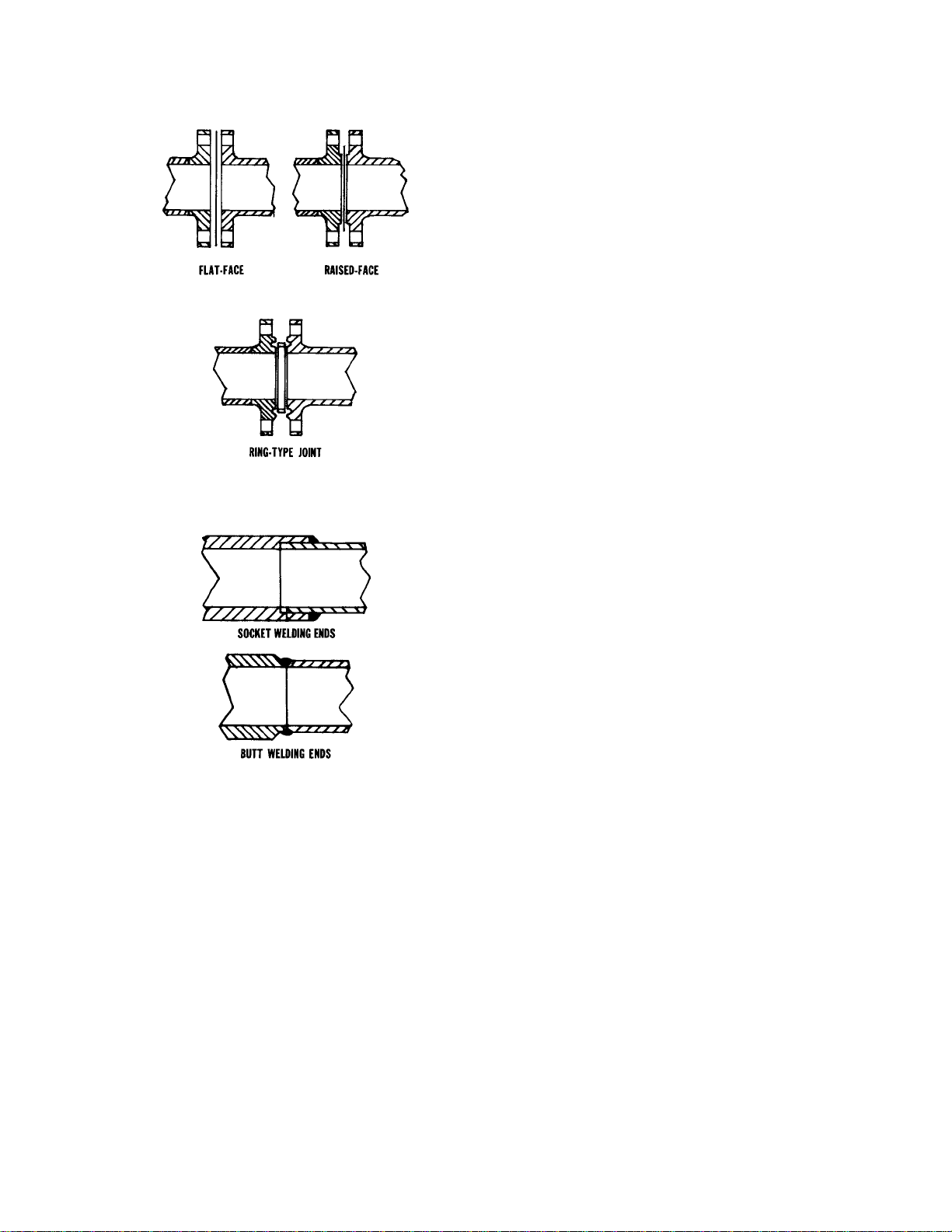
most common flanged end connections include
flat-face, raised-face, and ring-type joint.

The flat face variety allows the matching flanges to
be in full-face contact with the gasket clamped
between them. This construction is commonly
used in low pressure, cast iron, and brass valves,
and minimizes flange stresses caused by initial
bolting-up force.

The raised-face flange features a circular
raised-face with the inside diameter the same as
the valve opening, and the outside diameter less
than the bolt circle diameter. The raised-face is

1−7

or Monelt, but is available in almost any metal.
This makes an excellent joint at high pressures
and is used up to 15,000 psig (1034 bar),
however, it is generally not used at high
temperatures. It is furnished only on steel and
alloy valve bodies when specified.

Welding End Connections

Welding ends on control valves (figure 1-14) are
leak-tight at all pressures and temperatures, and
are economical in first cost. Welding end valves
are more difficult to take from the line and are
limited to weldable materials. Welding ends come
in two styles:

D Socket welding

A7098

Figure 1-13. Popular Varieties of

Bolted Flange Connections

A7099

Figure 1-14. Common Welded End Connections

finished with concentric circular grooves for
precise sealing and resistance to gasket blowout.
This kind of flange is used with a variety of gasket
materials and flange materials for pressures
through the 6000 psig (414 bar) pressure range
and for temperatures through 1500°F (815°C).
This style of flanging is normally standard on Class
250 cast iron bodies and all steel and alloy steel
bodies.

The ring-type joint flange is similar in looks to the
raised-face flange except that a U-shaped groove
is cut in the raised-face concentric with the valve
opening. The gasket consists of a metal ring with
either an elliptical or octagonal cross-section.
When the flange bolts are tightened, the gasket is
wedged into the groove of the mating flange and a
tight seal is made. The gasket is generally soft iron

D Buttwelding

The socket welding ends are prepared by boring in
a socket at each end of the valve with an inside
diameter slightly larger than the pipe outside
diameter. The pipe slips into the socket where it
butts against a shoulder and then joins to the valve
with a fillet weld. Socket welding ends in a given
size are dimensionally the same regardless of pipe
schedule. They are usually furnished in sizes
through NPS 2.

The buttwelding ends are prepared by beveling
each end of the valve to match a similar bevel on
the pipe. The two ends are then butted to the
pipeline and joined with a full penetration weld.
This type of joint is used on all valve styles and the
end preparation must be different for each
schedule of pipe. These are generally furnished for
control valves in NPS 2-1/2 and larger. Care must
be exercised when welding valve bodies in the
pipeline to prevent excessive heat transmitted to
valve trim parts. Trims with low-temperature
composition materials must be removed before
welding.

Valve Body Bonnets

The bonnet of a control valve is the part of the
body assembly through which the valve plug stem
or rotary shaft moves. On globe or angle bodies, it
is the pressure retaining component for one end of
the valve body. The bonnet normally provides a
means of mounting the actuator to the body and
houses the packing box. Generally, rotary valves
do not have bonnets. (On some rotary-shaft
valves, the packing is housed within an extension
of the valve body itself, or the packing box is a
separate component bolted between the valve
body and bonnet.)

1−8

W0989

Figure 1-15. Typical Bonnet, Flange,

and Stud Bolts

guides the valve plug to ensure proper valve plug
stem alignment with the packing.

As mentioned previously, the conventional bonnet
on a globe-type control valve houses the packing.
The packing is most often retained by a packing
follower held in place by a flange on the yoke boss
area of the bonnet (figure 1-15). An alternate
packing retention means is where the packing
follower is held in place by a screwed gland (figure
1-3). This alternate is compact, thus, it is often
used on small control valves, however, the user
cannot always be sure of thread engagement.
Therefore, caution should be used if adjusting the
packing compression when the control valve is in
service.

Most bolted-flange bonnets have an area on the
side of the packing box which can be drilled and
tapped. This opening is closed with a standard
pipe plug unless one of the following conditions
exists:

D It is necessary to purge the valve body and
bonnet of process fluid, in which case the opening
can be used as a purge connection.

On a typical globe-style control valve body, the
bonnet is made of the same material as the valve
body or is an equivalent forged material because it
is a pressure-containing member subject to the
same temperature and corrosion effects as the
body. Several styles of valve body-to-bonnet
connections are illustrated. The most common is
the bolted flange type shown in figure 1-15. A
bonnet with an integral flange is also illustrated in
figure 1-15. Figure 1-3 illustrates a bonnet with a
separable, slip-on flange held in place with a split
ring. The bonnet used on the high pressure globe
valve body illustrated in figure 1-4, is screwed into
the valve body. Figure 1-8 illustrates a rotary-shaft
control valve in which the packing is housed within
the valve body and a bonnet is not used. The
actuator linkage housing is not a pressure­containing part and is intended to enclose the
linkage for safety and environmental protection.

On control valve bodies with cage- or retainer-style
trim, the bonnet furnishes loading force to prevent
leakage between the bonnet flange and the valve
body, and also between the seat ring and the
valve body. The tightening of the body-bonnet
bolting compresses a flat sheet gasket to seal the
body-bonnet joint, compresses a spiral-wound
gasket on top of the cage, and compresses an
additional flat sheet gasket below the seat ring to
provide the seat ring-body seal. The bonnet also
provides alignment for the cage, which, in turn,

D The bonnet opening is being used to detect
leakage from the first set of packing or from a
failed bellows seal.

Extension Bonnets

Extension bonnets are used for either high or low
temperature service to protect valve stem packing
from extreme process temperatures. Standard
PTFE valve stem packing is useful for most
applications up to 450°F (232°C). However, it is
susceptible to damage at low process
temperatures if frost forms on the valve stem. The
frost crystals can cut grooves in the PTFE, thus,
forming leakage paths for process fluid along the
stem. Extension bonnets remove the packing box
of the bonnet far enough from the extreme
temperature of the process that the packing
temperature remains within the recommended
range.

Extension bonnets are either cast (figure 1-16) or
fabricated (figure 1-17). Cast extensions offer
better high temperature service because of greater
heat emissivity, which provides better cooling
effect. Conversely, smooth surfaces that can be
fabricated from stainless steel tubing are preferred
for cold service because heat influx is usually the
major concern. In either case, extension wall
thickness should be minimized to cut down heat
transfer. Stainless steel is usually preferable to

1−9

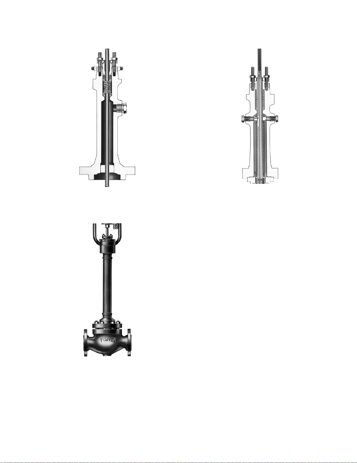
W0667-2

Figure 1-16. Extension Bonnet

W1416

Figure 1-17. Valve Body with

Fabricated Extension Bonnet

W6434

Figure 1-18. ENVIRO-SEALt Bellows

Seal Bonnet

Bellows Seal Bonnets

Bellows seal bonnets (figure 1-18) are used when
no leakage (less than 1x10−6 cc/sec of helium)
along the stem can be tolerated. They are often
used when the process fluid is toxic, volatile,
radioactive, or highly expensive. This special
bonnet construction protects both the stem and the
valve packing from contact with the process fluid.
Standard or environmental packing box
constructions above the bellows seal unit will
prevent catastrophic failure in case of rupture or
failure of the bellows.

As with other control valve pressure/ temperature
limitations, these pressure ratings decrease with
increasing temperature. Selection of a bellows
seal design should be carefully considered, and
particular attention should be paid to proper
inspection and maintenance after installation. The
bellows material should be carefully considered to
ensure the maximum cycle life.

Two types of bellows seal designs are used for
control valves:

D Mechanically formed as shown in figure 1-19

carbon steel because of its lower coefficient of
thermal conductivity. On cold service applications,
insulation can be added around the extension to
protect further against heat influx.

1−10

D Welded leaf bellows as shown in figure 1-20
The welded-leaf design offers a shorter total

package height. Due to its method of manufacture
and inherent design, service life may be limited.

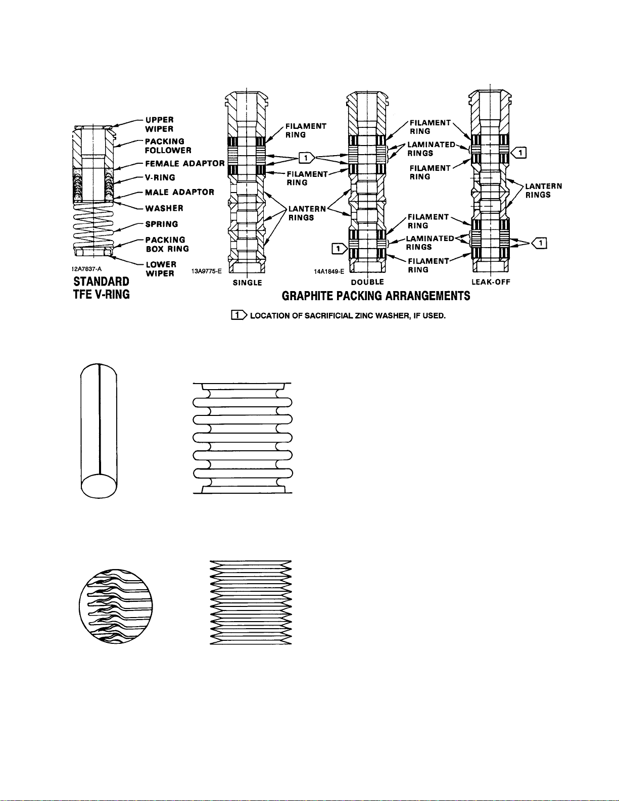
B2565

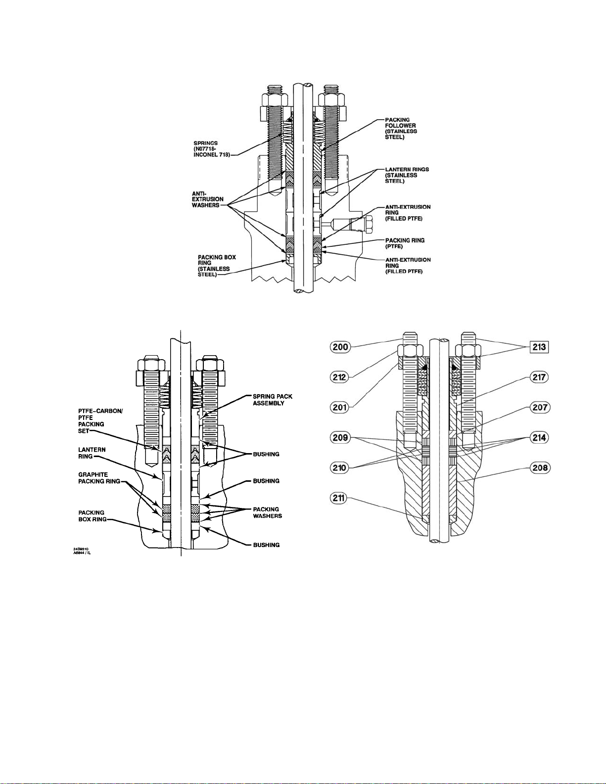
Figure 1-21. Comprehensive Packing Material Arrangements

for Globe-Style Valve Bodies

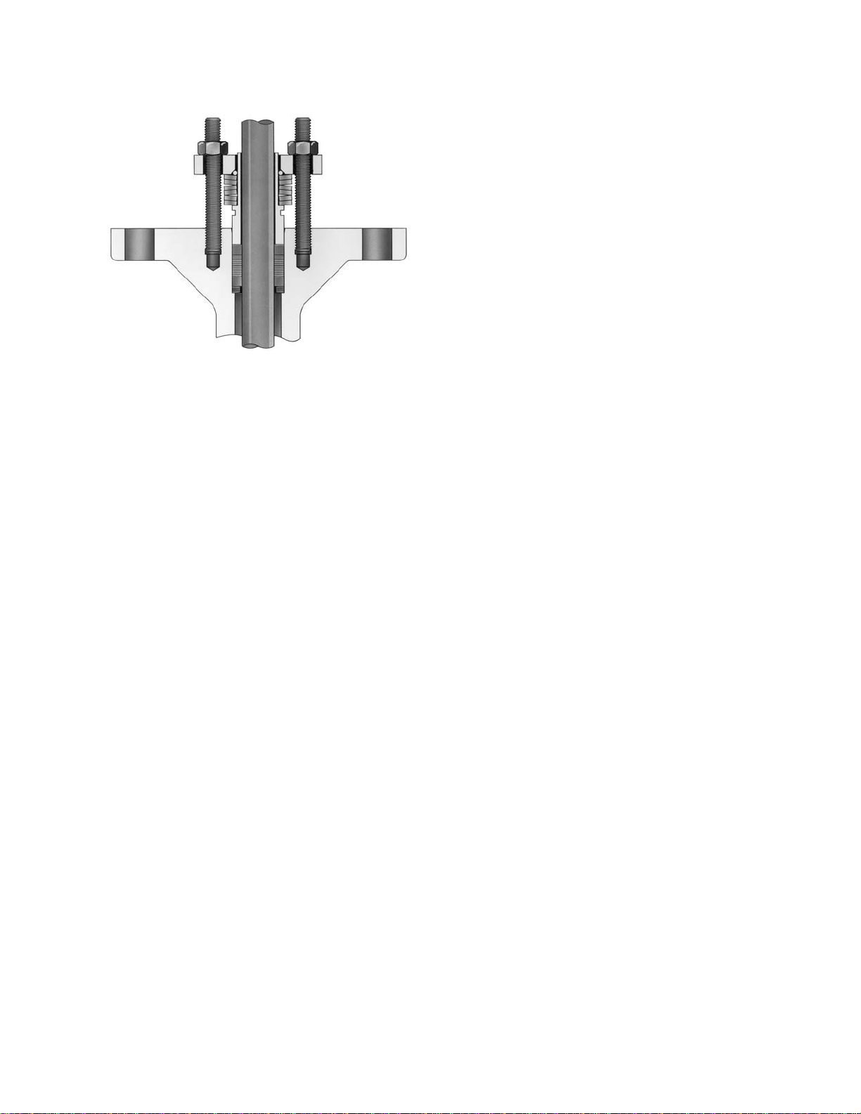
Control Valve Packing

Most control valves use packing boxes with the
packing retained and adjusted by a flange and
stud bolts (figure 1-27). Several packing materials
can be used depending upon the service
conditions expected and whether the application
requires compliance to environmental regulations.
Brief descriptions and service condition guidelines
for several popular materials and typical packing
material arrangements are shown in figure 1-21.

A5954

Figure 1-19. Mechanically Formed Bellows

A5955

Figure 1-20. Welded Leaf Bellows

The mechanically formed bellows is taller in
comparison and is produced with a more
repeatable manufacturing process.

PTFE V-Ring

D Plastic material with inherent ability to
minimize friction.

D Molded in V-shaped rings that are spring
loaded and self-adjusting in the packing box.
Packing lubrication not required.

D Resistant to most known chemicals except
molten alkali metals.

D Requires extremely smooth (2 to 4
micro-inches RMS) stem finish to seal properly.
Will leak if stem or packing surface is damaged.

D Recommended temperature limits: −40°F to
+450°F (−40°C to +232°C)

D Not suitable for nuclear service because
PTFE is easily destroyed by radiation.

1−11

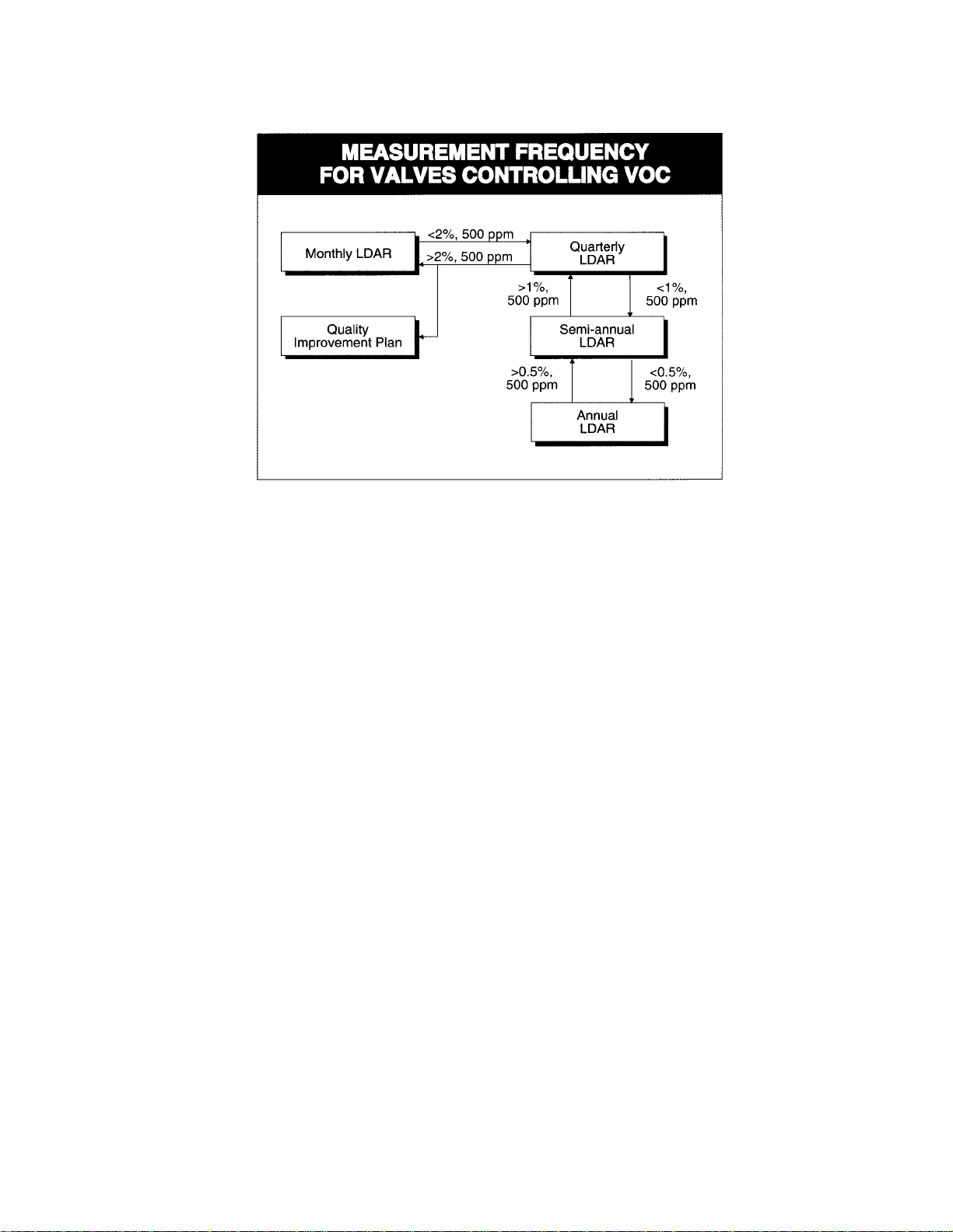
B2566

Figure 1-22. Measurement Frequency for Valves

Controlling Volatile Organic Chemicals (VOC)

Laminated and Filament Graphite

D Suitable for high temperature nuclear service
or where low chloride content is desirable (Grade
GTN).

D Provides leak-free operation, high thermal
conductivity, and long service life, but produces
high stem friction and resultant hysteresis.

D Impervious to most hard-to-handle fluids and
high radiation.

D Suitable temperature range: Cryogenic
temperatures to 1200°F (649°C).

D Lubrication not required, but an extension
bonnet or steel yoke should be used when packing
box temperature exceeds 800°F (427°C).

USA Regulatory Requirements for
Fugitive Emissions

Fugitive emissions are non-point source volatile
organic emissions that result from process
equipment leaks. Equipment leaks in the United
States have been estimated at over 400 million
pounds per year. Strict government regulations,
developed by the US, dictate Leak Detection and
Repair (LDAR) programs. Valves and pumps have
been identified as key sources of fugitive
emissions. In the case of valves, this is the

leakage to atmosphere due to packing seal or
gasket failures.

The LDAR programs require industry to monitor all
valves (control and noncontrol) at an interval that
is determined by the percentage of valves found to
be leaking above a threshold level of 500 ppmv
(some cities use a 100 ppmv criteria). This
leakage level is so slight you cannot see or hear it.
The use of sophisticated portable monitoring
equipment is required for detection. Detection
occurs by sniffing the valve packing area for
leakage using an Environmental Protection
Agency (EPA) protocol. This is a costly and
burdensome process for industry.

The regulations do allow for the extension of the
monitoring period for up to one year if the facility
can demonstrate an extremely low ongoing
percentage of leaking valves (less than 0.5% of
the total valve population). The opportunity to
extend the measurement frequency is shown in
figure 1-22.

Packing systems designed for extremely low
leakage requirements also extend packing seal life
and performance to support an annual monitoring
objective. The ENVIRO-SEALt packing system is
one example. Its enhanced seals incorporate four
key design principles including:

D Containment of the pliable seal material

through an anti-extrusion component.

1−12

D Proper alignment of the valve stem or shaft
within the bonnet bore.

D Applying a constant packing stress through
Belleville springs.

D Minimizing the number of seal rings to reduce
consolidation, friction, and thermal expansion.

The traditional valve selection process meant
choosing a valve design based upon its pressure
and temperature capabilities as well as its flow
characteristics and material compatibility. Valve
stem packing used in the valve was determined
primarily by the operating temperature in the
packing box area. The available material choices
included PTFE for temperatures below 93°C
(200°F) and graphite for higher temperature
applications.

Today, choosing a valve packing system has
become much more complex due to the number of
considerations one must take into account. For
example, emissions control requirements, such as
those imposed by the Clean Air Act within the
United States and by other regulatory bodies,
place tighter restrictions on sealing performance.
Constant demands for improved process output
mean that the valve packing system must not
hinder valve performance. Also, today’s trend
toward extended maintenance schedules dictates
that valve packing systems provide the required
sealing over longer periods.

In addition, end user specifications that have
become de facto standards, as well as standards
organizations specifications, are used by
customers to place stringent fugitive emissions
leakage requirements and testing guidelines on
process control equipment vendors. Emerson
Process Management and its observance of
limiting fugitive emissions is evident by its reliable
valve sealing (packing and gasket) technologies,
global emissions testing procedures, and
emissions compliance approvals.

A6161-1

Figure 1-23. Single PTFE V-Ring Packing

Single PTFE V-Ring Packing (Fig.
1-23)

The single PTFE V-ring arrangement uses a coil
spring between the packing and packing follower.
It meets the 100 ppmv criteria, assuming that the
pressure does not exceed 20.7 bar (300 psi) and
the temperature is between −18°C and 93°C (0°F
and 200°F). It offers excellent sealing performance
with the lowest operating friction.

ENVIRO-SEAL PTFE Packing
(Fig. 1-24)

The ENVIRO-SEAL PTFE packing system is an
advanced packing method that utilizes a compact,
live-load spring design suited to environmental
applications up to 51.7 bar and 232°C (750 psi
and 450°F). While it most typically is thought of as
an emission-reducing packing system,
ENVIRO-SEAL PTFE packing is, also, well-suited
for non-environmental applications involving high
temperatures and pressures, yielding the benefit of
longer, ongoing service life.

ENVIRO-SEAL Duplex Packing
(Fig. 1-25)

Given the wide variety of valve applications and
service conditions within industry, these variables
(sealing ability, operating friction levels, operating
life) are difficult to quantify and compare. A proper
understanding requires a clarification of trade
names.

This special packing system provides the
capabilities of both PTFE and graphite
components to yield a low friction, low emission,
fire-tested solution (API Standard 589) for
applications with process temperatures up to
232°C (450°F).

1−13

A6163

Figure 1-24. ENVIRO-SEAL PTFE Packing System

Figure 1-25. ENVIRO-SEAL Duplex (PTFE and

Graphite) Packing System

39B4612-A

Figure 1-26. ENVIRO-SEAL Graphite

ULF Packing System

carbon fiber reinforced TFE, is suited to 260°C
(500°F) service.

KALREZt Valve Stem Packing (KVSP)
systems

The KVSP pressure and temperature limits
referenced are for Fisher valve applications only.
KVSP with PTFE is suited to environmental use up
to 24.1 bar and 204°C (350 psi and 400°F) and, to
some non-environmental services up to 103 bar
(1500 psi). KVSP with ZYMAXXt, which is a

1−14

ENVIRO-SEAL Graphite Ultra Low
Friction (ULF) Packing (Fig. 1-26)

This packing system is designed primarily for
environmental applications at temperatures in
excess of 232°C (450°F). The patented ULF
packing system incorporates thin PTFE layers
inside the packing rings and thin PTFE washers on
each side of the packing rings. This strategic

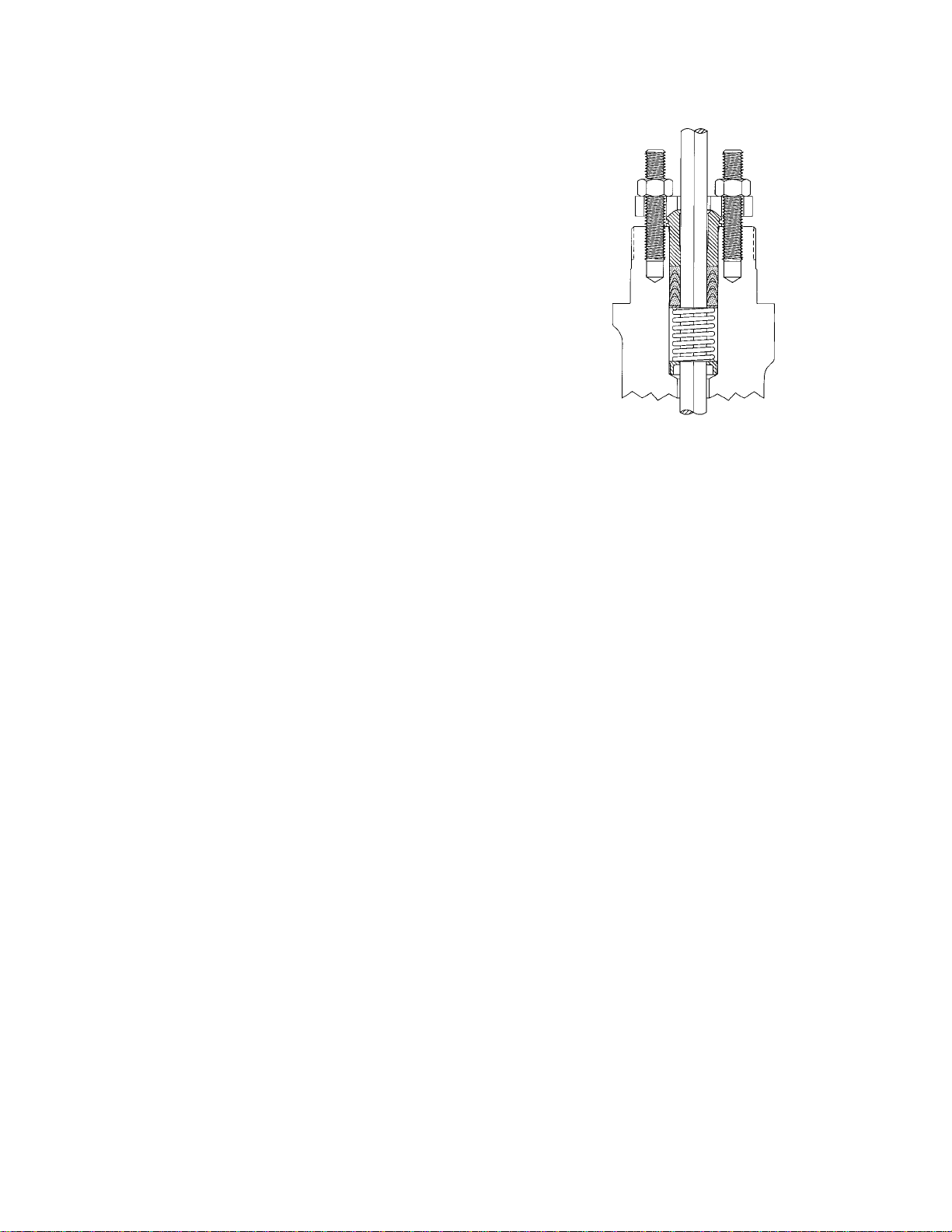
W6125-1

Figure 1-27. ENVIRO-SEAL Graphite

Packing System for Rotary Valves

placement of PTFE minimizes control problems,
reduces friction, promotes sealing, and extends
the cycle life of the packing set.

Braided graphite filament and double PTFE are
not acceptable environmental sealing solutions.

The following applies to rotary valves. In the case
of rotary valves, single PTFE and graphite ribbon
packing arrangements do not perform well as
fugitive emission sealing solutions.

The control of valve fugitive emissions and a
reduction in industry’s cost of regulatory
compliance can be achieved through these stem
sealing technologies.

While ENVIRO-SEAL packing systems have been
designed specifically for fugitive emission
applications, these technologies should also be
considered for any application where seal
performance and seal life have been an ongoing
concern or maintenance cost issue.

Characterization of Cage-Guided
Valve Bodies

HIGH-SEAL Graphite ULF Packing

Identical to the ENVIRO-SEAL graphite ULF
packing system below the packing follower, the
HIGH-SEAL system utilizes heavy-duty, large
diameter Belleville springs. These springs provide
additional follower travel and can be calibrated
with a load scale for a visual indication of packing
load and wear.

ENVIRO-SEAL Graphite Packing for
Rotary Valves (Fig. 1-27)

ENVIRO-SEAL graphite packing is designed for
environmental applications from −6°C to 316°C
(20°F to 600°F) or for those applications where fire
safety is a concern. It can be used with pressures
to 103 bar (1500 psi) and still satisfy the 500 ppmv
EPA leakage criteria.

Graphite Ribbon Packing for Rotary
Valves

Graphite ribbon packing is designed for
non-environmental applications that span a wide
temperature range from −198°C to 538°C (−325°F
to 1000°F).

The following table provides a comparison of
various sliding-stem packing selections and a
relative ranking of seal performance, service life,
and packing friction for environmental applications.

In valve bodies with cage-guided trim, the shape of
the flow openings or windows in the wall of the
cylindrical cage determines flow characterization.
As the valve plug is moved away from the seat
ring, the cage windows are opened to permit flow
through the valve. Standard cages have been
designed to produce linear, equal-percentage, and
quick-opening inherent flow characteristics. Note
the differences in the shapes of the cage windows
shown in figure 1-28. The flow rate/travel
relationship provided by valves utilizing these
cages is equivalent to the linear, quick-opening,
and equal-percentage curves shown for contoured
valve plugs (figure 1-29).

Cage-guided trim in a control valve provides a
distinct advantage over conventional valve body
assemblies in that maintenance and replacement
of internal parts is simplified. The inherent flow
characteristic of the valve can easily be changed
by installing a different cage. Interchange of cages
to provide a different inherent flow characteristic
does not require changing the valve plug or seat
ring. The standard cages shown can be used with
either balanced or unbalanced trim constructions.
Soft seating, when required, is available as a
retained insert in the seat ring and is independent
of cage or valve plug selection.

Cage interchangeability can be extended to
specialized cage designs that provide noise
attenuation or combat cavitation. These cages
furnish a modified linear inherent flow
characteristic, but require flow to be in a specific

1−15

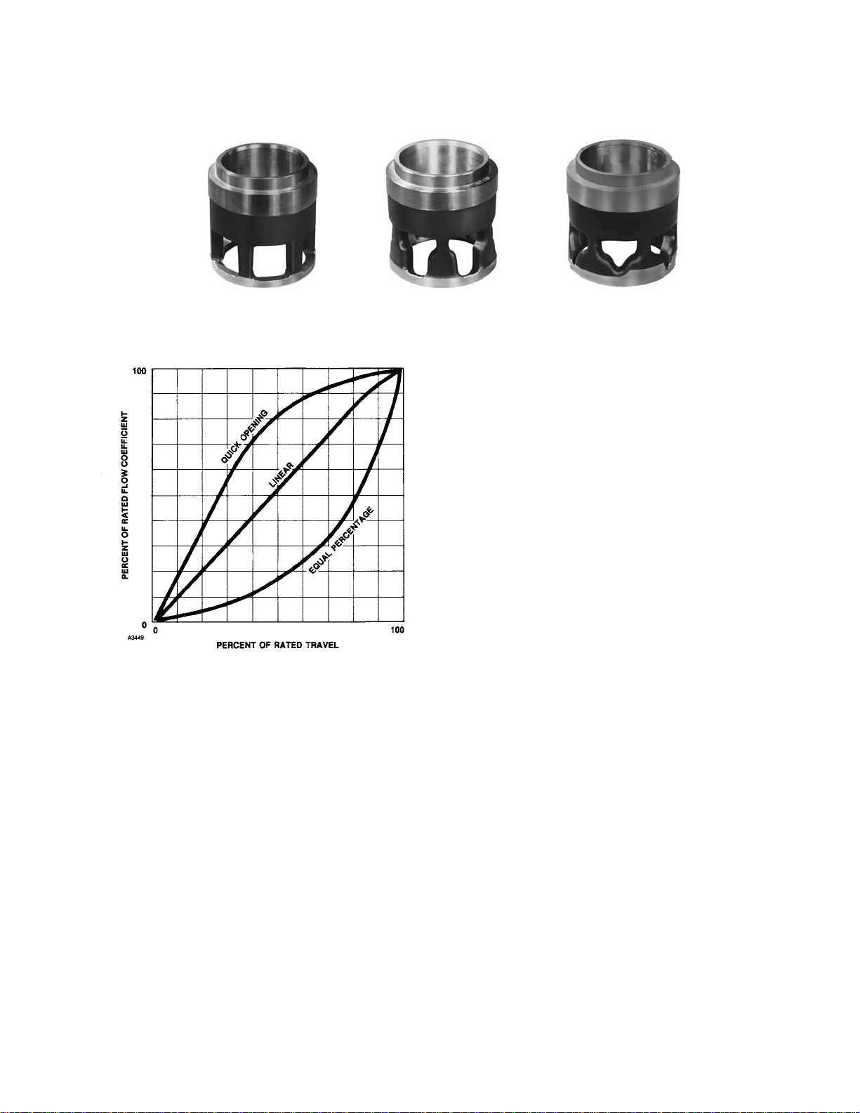
W0958 W0959 W0957

QUICK OPENING LINEAR EQUAL PERCENTAGE

Figure 1-28. Characterized Cages for Globe-Style Valve Bodies

Figure 1-29. Inherent Flow

Characteristics Curves

direction through the cage openings. Therefore, it
could be necessary to reverse the valve body in
the pipeline to obtain proper flow direction.

Characterized Valve Plugs

The valve plug, the movable part of a globe-style
control valve assembly, provides a variable
restriction to fluid flow. Valve plug styles are each
designed to:

D Provide a specific flow characteristic.

D Permit a specified manner of guiding or

alignment with the seat ring.

D Have a particular shutoff or
damage-resistance capability.

Valve plugs are designed for either two-position or
throttling control. In two-position applications, the
valve plug is positioned by the actuator at either of
two points within the travel range of the assembly.
In throttling control, the valve plug can be
positioned at any point within the travel range as
dictated by the process requirements.

The contour of the valve plug surface next to the
seat ring is instrumental in determining the
inherent flow characteristic of a conventional
globe-style control valve. As the actuator moves
the valve plug through its travel range, the
unobstructed flow area changes in size and shape
depending upon the contour of the valve plug.
When a constant pressure differential is
maintained across the valve, the changing
relationship between percentage of maximum flow
capacity and percentage of total travel range can
be portrayed (figure 1-29), and is designated as
the inherent flow characteristic of the valve.

Commonly specified inherent flow characteristics
include:

Linear Flow

D A valve with an ideal linear inherent flow
characteristic produces a flow rate directly
proportional to the amount of valve plug travel
throughout the travel range. For instance, at 50%
of rated travel, flow rate is 50% of maximum flow;
at 80% of rated travel, flow rate is 80% of
maximum; etc. Change of flow rate is constant
with respect to valve plug travel. Valves with a
linear characteristic are often specified for liquid
level control and for flow control applications
requiring constant gain.

Equal-Percentage Flow

D Ideally, for equal increments of valve plug
travel, the change in flow rate regarding travel may
be expressed as a constant percent of the flow

1−16

Valve Plug Guiding

Accurate guiding of the valve plug is necessary for
proper alignment with the seat ring and efficient
control of the process fluid. The common methods
used are listed below.

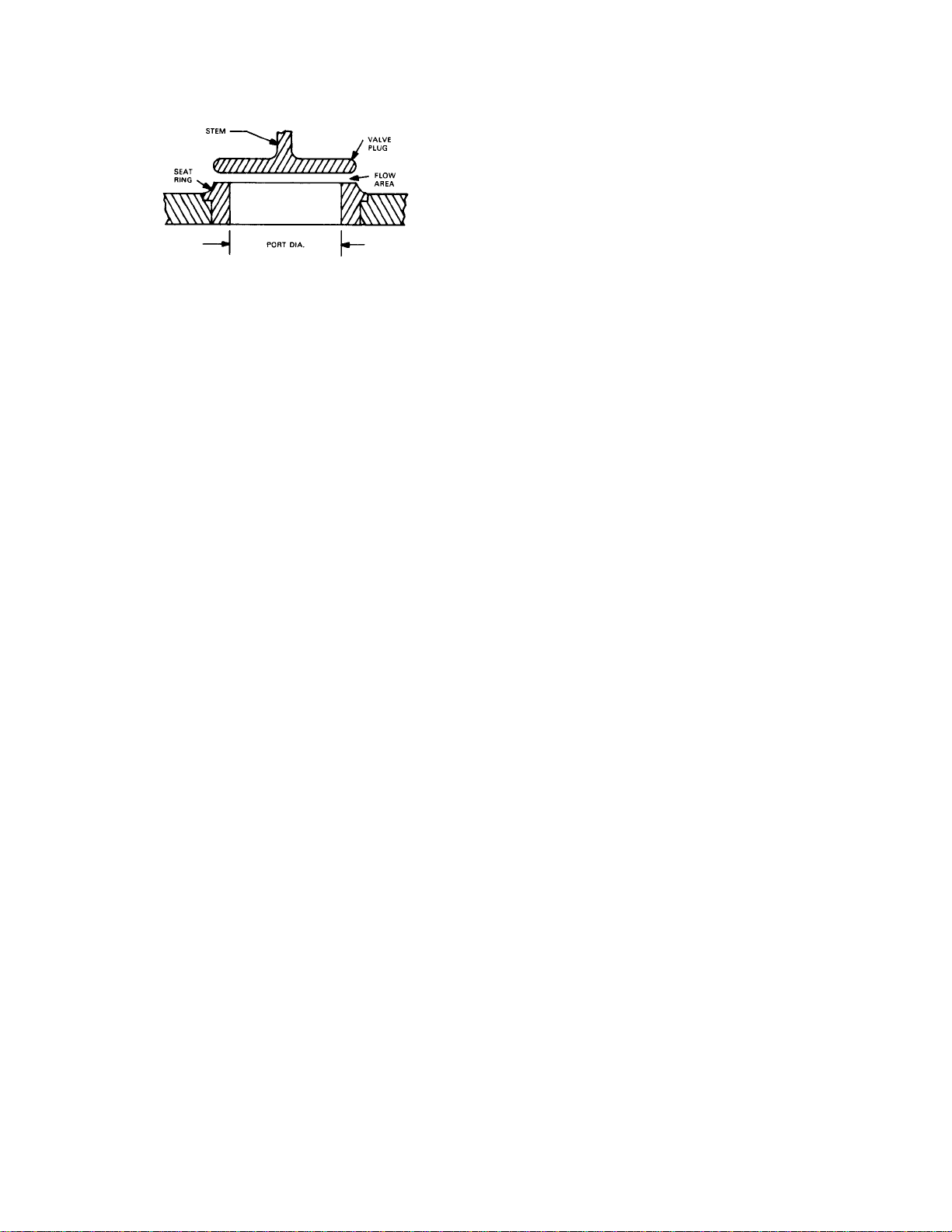
A7100

Figure 1-30. Typical Construction to Provide

Quick-Opening Flow Characteristic

rate at the time of the change. The change in flow
rate observed regarding travel will be relatively
small when the valve plug is near its seat, and
relatively high when the valve plug is nearly wide
open. Therefore, a valve with an inherent
equal-percentage flow characteristic provides
precise throttling control through the lower portion
of the travel range and rapidly increasing capacity
as the valve plug nears the wide-open position.
Valves with equal-percentage flow characteristics
are used on pressure control applications, on
applications where a large percentage of the
pressure drop is normally absorbed by the system
itself with only a relatively small percentage
available at the control valve, and on applications
where highly varying pressure drop conditions can
be expected. In most physical systems, the inlet
pressure decreases as the rate of flow increases,
and an equal percentage characteristic is
appropriate. For this reason, equal percentage
flow is the most common valve characteristic.

D Cage Guiding: The outside diameter of the
valve plug is close to the inside wall surface of the
cylindrical cage throughout the travel range. Since
the bonnet, cage, and seat ring are self-aligning
upon assembly, the correct valve plug and seat
ring alignment is assured when the valve closes
(figure 1-15).

D Top Guiding: The valve plug is aligned by a
single guide bushing in the bonnet, valve body
(figure 1-4), or by packing arrangement.

D Stem Guiding: The valve plug is aligned with
the seat ring by a guide bushing in the bonnet that
acts upon the valve plug stem (figure 1-3, left
view).

D Top-and-Bottom Guiding: The valve plug is
aligned by guide bushings in the bonnet and
bottom flange.

D Port Guiding: The valve plug is aligned by the
valve body port. This construction is typical for
control valves utilizing small-diameter valve plugs
with fluted skirt projections to control low flow rates
(figure 1-3, right view).

Quick-Opening Flow

D A valve with a quick opening flow
characteristic provides a maximum change in flow
rate at low travels. The curve is essentially linear
through the first 40 percent of valve plug travel,
then flattens out noticeably to indicate little
increase in flow rate as travel approaches the
wide-open position. Control valves with
quick-opening flow characteristics are often used
for on/off applications where significant flow rate
must be established quickly as the valve begins to
open. As a result, they are often utilized in relief
valve applications. Quick-opening valves can also
be selected for many of the same applications for
which linear flow characteristics are
recommended. This is because the quick-opening
characteristic is linear up to about 70 percent of
maximum flow rate. Linearity decreases
significantly after flow area generated by valve
plug travel equals the flow area of the port. For a
typical quick-opening valve (figure 1-30), this
occurs when valve plug travel equals one-fourth of
port diameter.

Restricted-Capacity Control Valve
Trim

Most control valve manufacturers can provide
valves with reduced- or restricted- capacity trim
parts. The reduced flow rate might be desirable for
any of the following reasons:

D Restricted capacity trim may make it possible
to select a valve body large enough for increased
future flow requirements, but with trim capacity
properly sized for present needs.

D Valves can be selected for adequate
structural strength, yet retain reasonable
travel/capacity relationship.

D Large bodies with restricted capacity trim can
be used to reduce inlet and outlet fluid velocities.

D Purchase of expensive pipeline reducers can
be avoided.

D Over-sizing errors can be corrected by use of
restricted capacity trim parts.

1−17

Conventional globe-style valve bodies can be fitted
with seat rings with smaller port size than normal
and valve plugs sized to fit those smaller ports.
Valves with cage-guided trim often achieve the
reduced capacity effect by utilizing valve plug,
cage, and seat ring parts from a smaller valve size
of similar construction and adapter pieces above
the cage and below the seat ring to mate those
smaller parts with the valve body (figure 1-28).
Because reduced capacity service is not unusual,
leading manufacturers provide readily available
trim part combinations to perform the required
function. Many restricted capacity trim
combinations are designed to furnish
approximately 40% of full-size trim capacity.

General Selection Criteria

Most of the considerations that guide the selection
of valve type and brand are rather basic. However,
there are some matters that may be overlooked by
users whose familiarity is mainly limited to just one
or a few valve types. Table 1-1 below provides a
checklist of important criteria; each is discussed at
length following the table.

Table 1-1. Suggested General Criteria for Selecting Type

and Brand of Control Valve

Body pressure rating
High and low temperature limits
Material compatibility and durability
Inherent flow characteristic and rangeability
Maximum pressure drop (shutoff and flowing)
Noise and cavitation
End connections
Shutoff leakage
Capacity versus cost
Nature of flowing media
Dynamic performance

Pressure Ratings

Body pressure ratings ordinarily are considered
according to ANSI pressure classes — the most
common ones for steel and stainless steel being
Classes 150, 300 and 600. (Source documents
are ASME/ANSI Standards B16.34, “Steel
Valves,” and ANSI B16.1, “Cast Iron Pipe
Flanges and Flanged Fittings.”) For a given body
material, each NSI Class corresponds to a
prescribed profile of maximum pressures that
decrease with temperature according to the
strength of the material. Each material also has a

minimum and maximum service temperature
based upon loss of ductility or loss of strength. For
most applications, the required pressure rating is
dictated by the application. However, because all
products are not available for all ANSI Classes, it
is an important consideration for selection.

Temperature Considerations

Required temperature capabilities are also a
foregone conclusion, but one that is likely to
narrow valve selection possibilities. The
considerations include the strength or ductility of
the body material, as well as relative thermal
expansion of various parts.

Temperature limits also may be imposed due to
disintegration of soft parts at high temperatures or
loss of resiliency at low temperatures. The soft
materials under consideration include various
elastomers, plastics, and PTFE. They may be
found in parts such as seat rings, seal or piston
rings, packing, rotary shaft bearings and butterfly
valve liners. Typical upper temperature limits for
elastomers are in the 200 - 350°F range, and the
general limit for PTFE is 450°F.

Temperature affects valve selection by excluding
certain valves that do not have high or low
temperature options. It also may have some affect
on the valve’s performance. For instance, going
from PTFE to metal seals for high temperatures
generally increases the shutoff leakage flow.
Similarly, high temperature metal bearing sleeves
in rotary valves impose more friction upon the
shaft than do PTFE bearings, so that the shaft
cannot withstand as high a pressure-drop load at
shutoff. Selection of the valve packing is also
based largely upon service temperature.

Material Selection

The third criterion in table 1-1, “material
compatibility and durability”, is a more complex
consideration. Variables may include corrosion by
the process fluid, erosion by abrasive material,
flashing, cavitation or pressure and temperature
requirements. The piping material usually indicates
the body material. However, because the velocity
is higher in valves, other factors must be
considered. When these variables are included,
often valve and piping materials will differ. The trim
materials, in turn, are usually a function of the
body material, temperature range and qualities of
the fluid. When a body material other than carbon,
alloy, or stainless steel is required, use of an
alternate valve type, such as lined or bar stock,
should be considered.

1−18

Flow Characteristic

The next selection criterion, “inherent flow
characteristic”, refers to the pattern in which the
flow at constant pressure drop changes according
to valve position. Typical characteristics are
quick-opening, linear, and equal-percentage. The
choice of characteristic may have a strong
influence upon the stability or controllability of the
process (see table 1-3), as it represents the
change of valve gain relative to travel.

Most control valves are carefully “characterized”
by means of contours on a plug, cage, or ball
element. Some valves are available in a variety of
characteristics to suit the application, while others
offer little or no choice. To quantitatively determine
the best flow characteristic for a given application,
a dynamic analysis of the control loop can be
performed. In most cases, however, this is
unnecessary; reference to established rules of
thumb will suffice.

The accompanying drawing illustrates typical flow
characteristic curves (figure 1-29). The quick
opening flow characteristic provides for maximum
change in flow rate at low valve travels with a fairly
linear relationship. Additional increases in valve
travel give sharply reduced changes in flow rate,
and when the valve plug nears the wide open
position, the change in flow rate approaches zero.
In a control valve, the quick opening valve plug is
used primarily for on-off service; but it is also
suitable for many applications where a linear valve
plug would normally be specified.

Rangeability

operating stability. To a certain extent, a valve with
one inherent flow characteristic can also be made
to perform as though it had a different
characteristic by utilizing a nonlinear (i.e.,
characterized) positioner-actuator combination.
The limitation of this approach lies in the
positioner’s frequency response and phase lag
compared to the characteristic frequency of the
process. Although it is common practice to utilize a
positioner on every valve application, each
application should be reviewed carefully. There
are certain examples of high gain processes
where a positioner can hinder valve performance.

Pressure Drop

The maximum pressure drop a valve can tolerate
at shutoff, or when partially or fully open, is an
important selection criteria. Sliding-stem valves
are generally superior in both regards because of
the rugged nature of their moving parts. Many
rotary valves are limited to pressure drops well
below the body pressure rating, especially under
flowing conditions, due to dynamic stresses that
high velocity flow imposes on the disk or ball
segment.

Noise and Cavitation

Noise and cavitation are two considerations that
often are grouped together because both result
from high pressure drops and large flow rates.
They are treated by special modifications to
standard valves. Chapter four discusses the
cavitation phenomenon and its impact and
treatment, while chapter six discusses noise
generation and abatement.

Another aspect of a valve’s flow characteristic is its
rangeability, which is the ratio of its maximum and
minimum controllable flow rates. Exceptionally
wide rangeability may be required for certain
applications to handle wide load swings or a
combination of start-up, normal and maximum
working conditions. Generally speaking, rotary
valves—especially partial ball valves—have
greater rangeability than sliding-stem varieties.

Use of Positioners

A positioner is an instrument that helps improve
control by accurately positioning a control valve
actuator in response to a control signal. They are
useful in many applications and are required with
certain actuator styles in order to match actuator
and instrument pressure signals, or to provide

End Connections

The three common methods of installing control
valves in pipelines are by means of screwed pipe
threads, bolted flanges, and welded end
connections. At some point in the selection
process, the valve’s end connections must be
considered with the question simply being whether
the desired connection style is available in the
valve being considered.

In some situations, this matter can limit the
selection rather narrowly. For instance, if a piping
specification calls for welded connections only, the
choice usually is limited to sliding-stem valves.

Screwed end connections, popular in small control
valves, offer more economy than flanged ends.

1−19

The threads usually specified are tapered female
NPT on the valve body. They form a
metal-to-metal seal by wedging over the mating
male threads on the pipeline ends. This
connection style is usually limited to valves not
larger than NPS 2, and is not recommended for
elevated temperature service.

Valve maintenance might be complicated by
screwed end connections if it is necessary to take
the body out of the pipeline. Screwed connections
require breaking a flanged joint or union
connection to permit unscrewing the valve body
from the pipeline.

Flanged end valves are easily removed from the
piping and are suitable for use through the range
of working pressures that most control valves are
manufactured (figure 1-13).

Flanged end connections can be utilized in a
temperature range from absolute zero (−273°F) to
approximately 1500°F (815°C). They are utilized
on all valve sizes. The most common flanged end
connections include flat face, raised face, and ring
type joint.

the trim. Special precautions in seat material
selection, seat preparation and seat load are
necessary to ensure success.

Flow Capacity

Finally, the criterion of capacity or size can be an
overriding constraint on selection. For extremely
large lines, sliding-stem valves are more
expensive than rotary types. On the other hand,
for extremely small flows, a suitable rotary valve
may not be available. If future plans call for
significantly larger flow, then a sliding-stem valve
with replaceable restricted trim may be the
answer. The trim can be changed to full size trim
to accommodate higher flow rates at less cost than
replacing the entire valve body assembly.

Rotary style products generally have much higher
maximum capacity than sliding-stem valves for a
given body size. This fact makes rotary products
attractive in applications where the pressure drop
available is rather small. However, it is of little or
no advantage in high pressure drop applications
such as pressure regulation or letdown.

Welded ends on control valves are leak-tight at all
pressures and temperatures and are economical
in initial cost (figure 1-14). Welded end valves are
more difficult to remove from the line and are
limited to weldable materials. Welded ends come
in two styles, socket weld and buttweld.

Shutoff Capability

Some consideration must be given to a valve’s
shutoff capability, which is usually rated in terms of
classes specified in ANSI/FCI70-2 (table 1-4). In
service, shutoff leakage depends upon many
factors, including but not limited to, pressure drop,
temperature, and the condition of the sealing
surfaces. Because shutoff ratings are based upon
standard test conditions that can be different from
service conditions, service leakage cannot be
predicted accurately. However, the shutoff class
provides a good basis for comparison among
valves of similar configuration. It is not uncommon
for valve users to overestimate the shutoff class
required.

Because tight shutoff valves generally cost more
both in initial cost, as well as in later maintenance
expense, serious consideration is warranted. Tight
shutoff is particularly critical in high pressure
valves, considering that leakage in these
applications can lead to the ultimate destruction of

Conclusion

For most general applications, it makes sense
both economically, as well as technically, to use
sliding-stem valves for lower flow ranges, ball
valves for intermediate capacities, and high
performance butterfly valves for the very largest
required flows. However, there are numerous
other factors in selecting control valves, and
general selection principles are not always the
best choice.

Selecting a control valve is more of and art than a
science. Process conditions, physical fluid
phenomena, customer preference, customer
experience, supplier experience, among numerous
other criteria must be considered in order to obtain
the best possible solution. Many applications are
beyond that of general service, and as chapter 4
will present, there are of number of selection
criteria that must be considered when dealing with
these sometimes severe flows.

Special considerations may require out-of-the­ordinary valve solutions; there are valve designs
and special trims available to handle high noise
applications, flashing, cavitation, high pressure,
high temperature and combinations of these
conditions.

1−20

After going through all the criteria for a given
application, the selection process may point to
several types of valves. From there on, selection
becomes a matter of price versus capability,

institutional preferences. As no single control valve
package is cost-effective over the full range of
applications, it is important to keep an open mind
to alternative choices.

coupled with the inevitable personal and

Table 1-2. Major Categories and Subcategories of Control Valves with Typical General Characteristics

Valve Style

Regular

Sliding-stem

Bar Stock

Economy

Sliding-stem

Thru-Bore

Ball

Partial Ball

Eccentric Plug Erosion Resistance 1 to 8

Swing-Thru

Butterfly

Lined Butterfly

High

Performance

Butterfly

Main

Characteristics

Heavy Duty

Versatile

Machined from Bar

Stock

Light Duty

Inexpensive

On-Of f Service 1 to 24

Characterized for

Throttling

No Seal 2 to 96

Elastomer or

TFE Liner

Offset Disk

General Service

Typical Size

Range,
inches

1 to 24

½ to 3

½ to 2

1 to 24

2 to 96

2 to 72

Typical

Standard Body

Materials

Carbon Steel

Cast Iron
Stainless

Variety of Alloys

Bronze

Cast Iron

Carbon Steel
Carbon Steel

Stainless

Carbon Steel

Stainless

Carbon Steel

Stainless

Carbon Steel

Cast Iron
Stainless

Carbon Steel

Cast Iron
Stainless

Carbon Steel

Stainless

Typical Standard

End Connection

ANSI Flanged

Welded

Screwed

Flangeless

Screwed

Screwed To ANSI 125 Moderate Good

Flangeless To ANSI 900 High Excellent
Flangeless

Flanged
Flanged To ANSI 600 Moderate Excellent

Flangeless

Lugged
Welded

Flangeless

Lugged

Flangeless

Lugged

Typical

Pressure

Ratings

To ANSI 2500 Moderate Excellent

To ANSI 600 Low Excellent

To ANSI 600 High Excellent

To ANSI 2500 High Poor

To ANSI 300 High Good

To ANSI 600 High Excellent

Relative Flow

Capacity

Relative

Shutoff

Capability

1−21

Table 1-3. Control Valve Characteristic Recommendations

Liquid Level Systems

Control Valve Pressure Drop

Constant ΔP Linear
Decreasing ΔP with increasing load, ΔP at maximum load > 20% of minimum load ΔP Linear
Decreasing ΔP with increasing load, ΔP at maximum load < 20% of minimum load ΔP Equal-percentage
Increasing ΔP with increasing load, ΔP at maximum load < 200% of minimum load ΔP Linear
Increasing ΔP with increasing load, ΔP at maximum load > 200% of minimum load ΔP Quick Opening

Best Inherent

Characteristic

Pressure Control Systems

Application

Liquid Process Equal-Percentage
Gas Process, Large Volume (Process has a receiver, Distribution System or Transmission Line Exceeding 100 ft. of

Nominal Pipe Volume), Decreasing ΔP with Increasing Load, ΔP at Maximum Load > 20% of Minimum Load ΔP Linear
Gas Process, Large Volume, Decreasing ΔP with Increasing Load, ΔP at Maximum Load < 20% of Minimum Load ΔP Equal-Percentage
Gas Process, Small Volume, Less than 10 ft. of Pipe between Control Valve and Load Valve Equal-Percentage

Best Inherent

Characteristic

Flow Control Processes

Application Best Inherent Characteristic

Flow Measurement Signal to

Controller

Proportional to Flow In Series Linear Equal-Percentage

Proportional to Flow Squared In Series Linear Equal-Percentage

*When control valve closes, flow rate increases in measuring element.

Location of Control Valve in Relation

to Measuring Element

In Bypass* Linear Equal-Percentage

In Bypass* Equal-Percentage Equal-Percentage

Wide Range of Flow Set Point

Small Range of Flow but

Large ΔP Change at Valve

with Increasing Load

1−22

Table 1-4. Control Valve Leakage Standards

ANSI

B16.104-1976

Class II 0.5% valve capacity at full travel Air

Class III 0.1% valve capacity at full travel Air

Class IV 0.01% valve capacity at full travel Air

Class V

Class VI

Copyright 1976 Fluid Controls Institute, Inc. Reprinted with permission.

Maximum Leakage Test Medium Pressure and Temperature

5 x 10-4 mL/min/psid/inch port dia. (5

-12 m3

x 10

/sec/Δbar/mm port dia)

Nominal Port

Diameter

In

1

1-1/2

2

2-1/2

3
4
6
8

mm

25
38
51
64

76
102
152
203

Bubbles per

Minute

1
2
3
4

6
11
27
45

Water

mL per Minute

0.15

0.30

0.45

0.60

0.90

1.70

4.00

6.75

Service ΔP or 50 psid (3.4 bar differential),

whichever is lower, at 50_ or 125_F (10_ to 52_C)

Service ΔP or 50 psid (3.4 bar differential),

whichever is lower, at 50_ or 125_F (10_ to 52_C)

Service ΔP or 50 psid (3.4 bar differential),

whichever is lower, at 50_ or 125_F (10_ to 52_C)

Service ΔP at 50_ or 125_F (10_ to 52_C)

Test

Medium

Pressure and Temperature

Service ΔP or 50 psid (3.4 bar

Air

differential), whichever is lower, at 50_

or 125_F (10_ to 52_C)

1−23

1−24

Chapter 2

Actuator Selection

The actuator is the distinguishing element that
differentiates control valves from other types of
valves. The first actuated valves were designed in
the late 19th century. Today, they would be better
described as regulators since they operated
directly from the process fluid. These “automatic
valves” were the mainstay of industry through the
early 1930s.

It was at this time that the first pneumatic
controllers were used. Development of valve
controllers and the adaptation of standardized
control signals stimulated design of the first, true,
control valve actuators.

The control valve industry has evolved to fill a
variety of needs and desires. Actuators are
available with an array of designs, power sources
and capabilities. Proper selection involves process
knowledge, valve knowledge, and actuator
knowledge.

A control valve can perform its function only as
well as the actuator can handle the static and
dynamic loads placed on it by the valve.
Therefore, proper selection and sizing are very
important. Since the actuator can represent a
significant portion of the total control valve price,
careful selection of actuator and accessory options
can lead to significant dollar savings.

The range of actuator types and sizes on the
market today is so great that it seems the selection
process might be highly complex. With a few rules
in mind and knowledge of fundamental needs, the
selection process can be simple.

The following parameters are key as they quickly
narrow the actuator choices:

D Power source availability
D Fail-safe requirements

D Torque or thrust requirements
D Control functions

Power Source Availability

The power source available at the location of a
valve can often point directly to what type of
actuator to choose. Typically, valve actuators are
powered either by compressed air or by electricity.
However, in some cases water pressure, hydraulic
fluid, or even pipeline pressure can be used.

Since most plants have both electricity and
compressed air readily available, the selection
depends upon the ease and cost of furnishing
either power source to the actuator location.
Reliability and maintenance requirements of the
power system must also be considered.
Consideration should also be given to providing
backup operating power to critical plant loops.

Fail-safe Requirements

The overall reliability of power sources is quite
high. However, many loops demand specific valve
action should the power source ever fail. Desired
action upon a signal failure may be required for
safety reasons or for protection of equipment.

Fail-safe systems store energy, either
mechanically in springs, pneumatically in volume
tanks, or in hydraulic accumulators. When power
fails, the fail-safe systems are triggered to drive
the valves to the required position and to then
maintain this position until returned to normal
operation. In many cases, the process pressure is
used to ensure or enhance this action.

www.Fisher.com

Actuator designs are available with a choice of
failure mode between failing open, failing closed,
or holding in the last position. Many actuator
systems incorporate failure modes at no extra
cost. For example, spring-and-diaphragm
actuators are inherently fail open or closed, while
electric operators typically hold their last position.

Torque or Thrust Requirements

An actuator must have sufficient thrust or torque
for the prescribed application. In some cases this
requirement can dictate actuator type as well as
power supply requirements.

For instance, large valves requiring a high thrust
may be limited to only electric or electro-hydraulic
actuators due to a lack of pneumatic actuators with
sufficient thrust capability. Conversely,
electro-hydraulic actuators would be a poor choice
for valves with very low thrust requirements.

The matching of actuator capability with valve
body requirements is best left to the control valve
manufacturer as there are considerable
differences in frictional and fluid forces from valve
to valve.

Throttling actuators have considerably higher
demands put on them from both a compatibility
and performance standpoint. A throttling actuator
receives its input from an electronic or pneumatic
instrument that measures the controlled process
variable. The actuator must then move the final
control element in response to the instrument
signal in an accurate and timely fashion to ensure
effective control. The two primary additional
requirements for throttling actuators include:

D Compatibility with instrument signal
D Better static and dynamic performance to

ensure loop stability
Compatibility with instrument signals is inherent in

many actuator types, or it can be obtained with
add-on equipment. But, the high-performance
characteristics required of a good throttling
actuator cannot be bolted on; instead, low
hysteresis and minimal deadband must be
designed into actuators.

Stroking speed, vibration, and temperature
resistance must also be considered if critical to the
application. For example, on liquid loops
fast-stroking speeds can be detrimental due to the
possibility of water hammer.

Vibration or mounting position can be a potential
problem. The actuator weight, combined with the
weight of the valve, may necessitate bracing.

Control Functions

Knowledge of the required actuator functions will
most clearly define the options available for
selection. These functions include the actuator
signal (pneumatic, electric, etc.), signal range,
ambient temperatures, vibration levels, operating
speed, frequency, and quality of control that is
required.

Signal types are typically grouped as such:

D Two-position (on-off)
D Analog (throttling)
D Digital

Two-position electric, electro-pneumatic, or
pneumatic switches control on-off actuators. This
is the simplest type of automatic control and the
least restrictive in terms of selection.

It is essential to determine the ambient
temperature and humidity that the actuator will
experience. Many actuators contain either
elastomeric or electronic components that can be
subject to degradation by high humidity or
temperature.

Economics

Evaluation of economics in actuator selection is a
combination of the following:

D Cost
D Maintenance
D Reliability

A simple actuator, such as a
spring-and-diaphragm, has few moving parts and
is easy to service. Its initial cost is low, and
maintenance personnel understand and are
comfortable working with them.

2−2

An actuator made specifically for a control valve
eliminates the chance for a costly performance
mismatch. An actuator manufactured by the valve
vendor and shipped with the valve will eliminate
separate mounting charges and ensure easier
coordination of spare parts procurement.
Interchangeable parts among varied actuators are
also important to minimize spare-parts inventory.

splined shaft end and then is rigidly clamped to the
shaft eliminates lost motion, is easy to
disassemble, and is capable of high torque.

Sliding stem actuators are rigidly fixed to valve
stems by threaded and clamped connections.
Because they don’t have any linkage points, and
their connections are rigid, they exhibit no lost
motion and have excellent inherent control
characteristics.

Actuator Designs

There are many types of actuators on the market,
most of which fall into five general categories:

D Spring-and-diaphragm
D Pneumatic piston
D Rack and Pinion
D Electric motor
D Electro-hydraulic

Each actuator design has weaknesses, strong
points and optimum uses. Most actuator designs
are available for either sliding stem or rotary valve
bodies. They differ only by linkages or motion
translators; the basic power sources are identical.

Most rotary actuators employ linkages, gears, or
crank arms to convert direct linear motion of a
diaphragm or piston into the 90-degree output
rotation required by rotary valves. The most
important consideration for control valve actuators
is the requirement for a design that limits the
amount of lost motion between internal linkage
and valve coupling.

Spring-and-Diaphragm Actuators

The most popular and widely used control valve
actuator is the pneumatic spring-and-diaphragm
style. These actuators are extremely simple and
offer low cost and high reliability. They normally
operate over the standard signal ranges of 3 to 15
psi or 6 to 30 psi, and therefore, are often suitable
for throttling service using instrument signals
directly.

Many spring-and-diaphragm designs offer either
adjustable springs and/or wide spring selections to
allow the actuator to be tailored to the particular
application. Because they have few moving parts
that may contribute to failure, they are extremely
reliable. Should they ever fail, maintenance is
extremely simple. Improved designs now include
mechanisms to control the release of spring
compression, eliminating possible personnel injury
during actuator disassembly.

Use of a positioner or booster with a
spring-and-diaphragm actuator can improve
control, but when improperly applied, can result in
poor control. Follow the simple guidelines
available for positioner applications and look for:

D Rugged, vibration-resistant construction

Rotary actuators are now available that employ
tilting pistons or diaphragms. These designs
eliminate most linkage points (and resultant lost
motion) and provide a safe, accurate and enclosed
package.

When considering an actuator design, it is also
necessary to consider the method by which it is
coupled to the drive shaft of the control valve.
Slotted connectors mated to milled shaft flats are
generally not satisfactory if any degree of
performance is required. Pinned connections, if
solidly constructed, are suitable for nominal torque
applications. A splined connector that mates to a

D Calibration ease

D Simple, positive feedback linkages

The overwhelming advantage of the
spring-and-diaphragm actuator is the inherent
provision for fail-safe action. As air is loaded on
the actuator casing, the diaphragm moves the
valve and compresses the spring. The stored
energy in the spring acts to move the valve back to
its original position as air is released from the
casing. Should there be a loss of signal pressure
to the instrument or the actuator, the spring can
move the valve to its initial (fail-safe) position.

2−3

DIAPHRAGM CASING

DIAPHRAGM

DIAPHRAGM
PLATE

LOWER DIAPHRAGM CASING

ACTUATOR SPRING

ACTUATOR STEM

SPRING SEAT

SPRING ADJUSTOR

STEM CONNECTOR

YOKE

TRAVEL INDICATOR DISK
INDICATOR SCALE

W0364-1

W0363-1

Figure 2-1. Spring-and-diaphragm actuators offer an excellent first choice for most control valves.

They are inexpensive, simple and have built-in, fail-safe action. Pictured above are cutaways of the popular

Fisher 667 (left) and Fisher 657 (right) actuators.

W0368-2

Figure 2-2. Spring-and-diaphragm actuators

can be supplied with a top-mounted handwheel.

The handwheel allows manual operation and also

acts as a travel stop or means of emergency

operation.

Actuators are available for either fail-open or
fail-closed action. The only drawback to the
spring-and-diaphragm actuator is a relatively
limited output capability. Much of the thrust
created by the diaphragm is taken up by the spring
and thus does not result in output to the valve.

Therefore, the spring-and-diaphragm actuator is
used infrequently for high force requirements. It is
not economical to build and use very large
spring-and-diaphragm actuators because the size,
weight and cost grow exponentially with each
increase in output force capability.

Piston Actuators

Piston actuators are generally more compact and
provide higher torque or force outputs than
spring-and-diaphragm actuators. Fisher piston
styles normally work with supply pressures
between 50 and 150 psi and can be equipped with
spring returns (however, this construction has
limited application).

Piston actuators used for throttling service must be
furnished with double-acting positioners that
simultaneously load and unload opposite sides of
the piston. The pressure differential created across
the piston causes travel toward the lower pressure
side. The positioner senses the motion, and when
the required position is reached, the positioner
equalizes the pressure on both sides of the piston.

The pneumatic piston actuator is an excellent
choice when a compact unit is required to produce
high torque or force. It is also easily adapted to

2−4

W9589-1 W9588-1

Figure 2-3. The Fisher 2052 spring-and-

diaphragm actuator has many features to provide

precise control. The splined actuator connection

features a clamped lever and single-joint linkage

to help eliminate lost motion.

W3827−1

W7447

Figure 2-5. Spring fail-safe is present in this

piston design. The Fisher 585C is an example of

a spring-bias piston actuator. Process pressure

can aid fail-safe action, or the actuator can be

configured for full spring-fail closure.

Figure 2-4. Double-acting piston actuators such

as the Fisher 1061 rotary actuator are a good

choice when thrust requirements exceed the

capability of spring-and-diaphragm actuators.
Piston actuators require a higher supply pressure,
but have benefits such as high stiffness and small

size. The 1061 actuator is typically used for

throttling service.

services where high ambient temperatures are a
concern.

The main disadvantages of piston actuators are
the high supply pressures required for positioners
when used in throttling service and the lack of
fail-safe systems.

W4102

Figure 2-6. Since the requirements for accuracy

and minimal lost motion are unnecessary for

on-off service, cost savings can be achieved by

simplifying the actuator design. The Fisher

1066SR incorporates spring-return capability.

There are two types of spring-return piston
actuators available. The variations are subtle, but
significant. It is possible to add a spring to a piston

2−5

actuator and operate it much like a spring-and­diaphragm. These designs use a single-acting
positioner that loads the piston chamber to move
the actuator and compress the spring. As air is
unloaded, the spring forces the piston back. These
designs use large, high output springs that are
capable of overcoming the fluid forces in the valve.

The alternative design uses a much smaller spring
and relies on valve fluid forces to help provide the
fail-safe action. In normal operation they act like a
double action piston. In a fail-safe situation the
spring initiates movement and is helped by
unbalance forces on the valve plug. These
actuators can be sized and set up to provide full
spring closure action without process assistance.

An alternative to springs is a pneumatic trip
system which often proves to be complex in
design, difficult to maintain and costly. While a trip
system is completely safe, any fail-safe
requirement consideration should be given first to
spring-and-diaphragm operators if they are
feasible.

Special care should be given during the selection
of throttling piston actuators to specify a design
that has minimal hysteresis and deadband. As the
number of linkage points in the actuator increases,
so does the deadband. As the number of sliding
parts increases, so does the hysteresis. An
actuator with high hysteresis and deadband can
be quite suitable for on-off service; however,
caution is necessary when attempting to adapt this
actuator to throttling service by merely bolting on a
positioner.

The cost of a spring-and-diaphragm actuator is
generally less than a comparable piston actuator.
Part of this cost saving is a result of the ability to
use instrument output air directly, thereby
eliminating the need for a positioner. The inherent
provision for fail-safe action in the spring-and­diaphragm actuator is also a consideration.

Rack and Pinion Actuators

W9479

Figure 2-7. The FieldQt actuator is a quarter
turn pneumatic rack and pinion actuator. It comes
with an integrated module combining the solenoid

and switchbox into a low profile, compact

package.

Electric Actuators

Electric actuators can be applied successfully in
many situations. Most electric operators consist of
motors and gear trains and are available in a wide
range of torque outputs, travels, and capabilities.
They are suited for remote mounting where no
other power source is available, for use where
there are specialized thrust or stiffness
requirements, or when highly precise control is
required.

Electric operators are economical versus
pneumatic actuators for applications in small size
ranges only. Larger units operate slowly and weigh
considerably more than pneumatic equivalents.
Available fail action is typically lock in last position.

One key consideration in choosing an electric
actuator is its capability for continuous closed-loop
control. In applications where frequent changes
are made in control-valve position, the electric
actuator must have a suitable duty cycle.

Rack and pinion actuators may come in a
double-acting design, or spring return, and are a
compact and economical solution for rotary shaft
valves. They provide high torque outputs and are
typically used for on-off applications with high
cycle life. They may also be used in processes
where higher variability is not a concern.

2−6

High performance electric actuators using
continuous rated DC motors and ball screw output
devices are capable of precise control and 100%
duty cycles.

Compared to other actuator designs, the electric
actuator generally provides the highest output

available within a given package size. Additionally,
electric actuators are stiff, that is, resistant to valve
forces. This makes them an excellent choice for
good throttling control of large, high-pressure
valves.

A. Unbalance Force

The unbalance force is that resulting from fluid
pressure at shutoff, and in the most general sense
can be expressed as:

Unbalance force = net pressure differential X net
unbalance area

Actuator Sizing

The last step in the selection process is to
determine the required actuator size.
Fundamentally, the process of sizing is to match
as closely as possible the actuator capabilities to
the valve requirements.

In practice, the mating of actuator and valve
requires the consideration of many factors. Valve
forces must be evaluated at the critical positions of
valve travel (usually open and closed) and
compared to actuator output. Valve force
calculation varies considerably between valve
styles and manufacturers. In most cases it is
necessary to consider a complex summation of
forces including:

D Static fluid forces
D Dynamic fluid forces and force gradients
D Friction of seals, bearings, and packing
D Seat loading

Although actuator sizing is not difficult, the great
variety of designs on the market and the ready
availability of vendor expertise (normally at no
cost) make detailed knowledge of the procedures
unnecessary.

Frequent practice is to take the maximum
upstream gauge pressure as the net pressure
differential unless the process design always
ensures a back pressure at the maximum inlet
pressure. Net unbalance area is the port area on a
single seated flow up design. Unbalance area may
have to take into account the stem area depending
on configuration. For balanced valves there is still
a small unbalance area. This data can be obtained
from the manufacturer. Typical port areas for
balanced valves flow up and unbalanced valves in
a flow down configuration are listed in table 2-1.

Table 2-1. Typical Unbalance Areas of Control Valves

Unbalance Area

Port Diameter,

Inches

1/4 0.049 – – –
3/8 0.110 – – –
1/2 0.196 – – –
3/4 0.441 – – –

1 0.785 – – –

1 5/16 1.35 0.04

1 7/8 2.76 0.062
2 5/16 4.20 0.27
3 7/16 9.28 0.118

4 3/8 15.03 0.154

7 38.48 0.81
8 50.24 0.86

Single-Seated

Unbalanced

Valves, In

2

Unbalance Area

Balanced Valves,

2

In

Actuator Spring for Globe Valves

The force required to operate a globe valve
includes:

A. Force to overcome static unbalance of the
valve plug

B. Force to provide a seat load
C. Force to overcome packing friction
D. Additional forces required for certain specific

applications or constructions
Total force required = A + B + C + D

B. Force to Provide Seat Load

Seat load, usually expressed in pounds per lineal
inch or port circumference, is determined by
shutoff requirements. Use the guidelines in table
2-2 to determine the seat load required to meet
the factory acceptance tests for ANSI/FCI 70-2
and IEC 534-4 leak Classes II through VI.

Because of differences in the severity of service
conditions, do not construe these leak
classifications and corresponding leakage rates as
indicators of field performance. To prolong seat life
and shutoff capabilities, use a higher than
recommended seat load. If tight shutoff is not a
prime consideration, use a lower leak class.

2−7

Table 2-2. Recommended Seat Load Per Leak Class for
Control Valves

Class I As required by customer

specification, no factory leak test
required

Class II 20 pounds per lineal inch of port

circumference

Class III 40 pounds per lineal inch of port

circumference

Class IV Standard (Lower) Seat only—40

pounds per lineal inch of port
circumference (up through a
4–3/8 inch diameter port)
Standard (Lower) Seat only—80
pounds per lineal inch of port
circumference (larger than 4–3/8
inch diameter port)

Class V Metal Seat—determine pounds

per lineal inch of port
circumference from figure 2-9

C. Packing Friction

Packing friction is determined by stem size,
packing type, and the amount of compressive load
placed on the packing by the process or the
bolting. Packing friction is not 100% repeatable in
its friction characteristics. Newer live loaded
packing designs can have significant friction forces
especially if graphite packing is used. Table 2-3
lists typical packing friction values.

D. Additional Forces

Additional forces to consider may include bellows
stiffness, unusual frictional forces resulting from
seals or special seating forces for soft metal seals.
The manufacturer should either supply this
information or take it into account when sizing an
actuator.

A2222−4/IL

Figure 2-8. Recommended Seat Load

pre-compression can be calculated as the
difference between the lower end of the bench set
(6 psig) and the beginning of the operating range
(3 psig). This 3 psig is used to overcome the
pre-compression so the net pre-compression force
must be:

3 psig X 100 sq. in. = 300 lbf.
This exceeds the force required and is an

adequate selection.

Actuator Force Calculations

Pneumatic spring-and-diaphragm actuators
provide a net force with the additional air pressure
after compressing the spring in air-to-close, or with
the net pre-compression of the spring in
air-to-open. This may be calculated in pounds per
square inch of pressure differential.

For example, suppose 275 pound-force (lbf) is
required to close the valve as calculated per the
process described earlier. An air-to-open actuator
with 100 square inches of diaphragm area and a
bench set of 6 to 15 psig is one available option.
The expected operating range is 3 to 15 psig. The

2−8

Piston actuators with springs are sized in the same
manner. The thrust from piston actuators without
springs can be calculated as:

Piston area X minimum supply pressure =
minimum available thrust
(maintain compatibility of units)

In some circumstances an actuator could supply
too much force and cause the stem to buckle, to
bend sufficiently to cause a leak, or to damage
valve internals.

The manufacturer normally takes responsibility for
actuator sizing and should have methods
documented to check for maximum stem loads.
Manufacturers also publish data on actuator
thrusts, effective diaphragm areas, and spring
data.

Table 2-3. Typical Packing Friction Values (Lb)

Stem Size

(Inches)

5/16 All 20 30 – – –

3/8 125

1/2 125

5/8 125

3/4 125

1 300

1–1/4 300

2 300

Values shown are frictional forces typically encountered when using standard
packing flange bolt-torquing procedures.

ANSI

Class

150
250
300

600
900

1500

150
250
300

600

900
1500
2500

150

250

300

600

150

250

300

600

900
1500
2500

600

900
1500
2500

600

900
1500
2500

600

900
1500
2500

PTFE Packing

Single Double

38 56 – – –

50 75 – – –

63 95 – – –

75 112.5 – – –

100 150 610

120 180 800

200 300 1225

Graphite

Ribbon/

Filament

125

– – –

190
250

320
380

180

– – –

230
320

410
500
590

218

– – –

290
400

350

– – –

440
660

880
1100
1320

850
1060
1300
1540

1100
1400
1700
2040

1725
2250
2750
3245

Torque Equations

Rotary valve torque equals the sum of a number of
torque components. To avoid confusion, a number
of these have been combined, and a number of
calculations have been performed in advance.
Thus, the torque required for each valve type can
be represented with two simple and practical
equations.

Breakout Torque

TB=A(DP

shutoff

)+B

Dynamic Torque

TD=C(DP

)

eff

Specific A, B, and C factors, for example, rotary
valve designs are included in tables 2-4 and 2-5.

Maximum Rotation

Maximum rotation is defined as the angle of valve
disk or ball in the fully open position.

Normally, maximum rotation is 90 degrees. The
ball or disk rotates 90 degrees from the closed
position to the wide-open position.

Some of the pneumatic spring-return piston and
pneumatic spring-and-diaphragm actuators are
limited to 60 or 75 degrees rotation.

For pneumatic spring-and-diaphragm actuators,
limiting maximum rotation allows for higher initial
spring compression, resulting in more actuator
breakout torque. Additionally, the effective length
of each actuator lever changes with valve rotation.
Published torque values, particularly for pneumatic
piston actuators, reflect this changing lever length.

Actuator Sizing for Rotary Valves

In selecting the most economical actuator for a
rotary valve, the determining factors are the torque
required to open and close the valve and the
torque output of the actuator.

This method assumes the valve has been properly
sized for the application and the application does
not exceed pressure limitations for the valve.

The Selection Process

In choosing an actuator type, the fundamental
requirement is to know your application. Control
signal, operating mode, power source available,
thrust/torque required, and fail-safe position can
make many decisions for you. Keep in mind
simplicity, maintainability and lifetime costs.

Safety is another consideration that must never be
overlooked. Enclosed linkages and controlled
compression springs available in some designs
are important for safety reasons. Table 2-6 lists
the pros and cons of the various actuator styles.

2−9

Table 2-4. Typical Rotary Shaft Valve Torque Factors V-Notch Ball Valve with Composition Seal

Fisher TCMt Plus Ball Seal

Valve Size,

NPS

1

1-1/2

2
3
4
6
8

10
12
14
16
16
20

1. PEEK/PTFE or metal/PTFE bearings.

Valve Shaft

Diameter,

Inches

1/2
5/8
5/8
3/4
3/4

1

1-1/4
1-1/4

1-1/2
1-3/4

2
2-1/8
2-1/2

Composition Bearings

Table 2-5. Typical High Performance Butterfly Torque Factors for Valve with Composition Seal

Valve Size Shaft Diameter

NPS Inch

2 1/2 0.30 100 1.05 2.45 515 515
3 5/8 0.56 150 3.59 10.8 1087 1028
4 3/4 0.99 232 7.65 21.2 1640 1551
6 1 2.30 438 17.5 46.7 4140 4140

8 1-1/4 4.80 705 33.4 223 7988 7552
10 1-1/4 8.10 1056 82.2 358 9792 9258
12 1-1/2 12.5 1470 106 626 12000 12000

A

(1)

0.07

0.12

0.19

0.10

0.10

1.80

1.80

1.80

4.00
42
60
60
97

PEEK/PTFE Bearings with PTFE Seal

A B

B

50
100
175
280
380
500
750

1250
3000
2400
2800
2800
5200

ANGLE OF OPENING S17400 H1075 S20910

60_ (K) 90_ (q) lbfSin lbfSin

60 Degrees 70 Degrees

0.38

1.10

1.30

0.15

1.10

1.10

3.80

3.80

11.0
75

105
105
190

C Maximum Allowable Torque

C

0.48

1.10

2.40

3.80

18.0

36.0

60.0
125

143
413
578
578

1044

Maximum TD,

LbfSIn.

515
1225
1225
2120
2120
4140
9820

9820

12,000
23,525
23,525
55,762
55,762

Table 2-6. Actuator Feature Comparison

Actuator Type Advantages Disadvantages

Spring-and-Diaphragm Lowest cost

Ability to throttle without positioner
Simplicity
Inherent fail-safe action
Low supply pressure requirement
Adjustable to varying conditions
Ease of maintenance

Pneumatic Piston High thrust capability

Compact
Lightweight
Adaptable to high ambient temperatures
Fast stroking speed
Relatively high actuator stiffness

Electric Motor Compactness

Very high stiffness
High output capability

Electro-Hydraulic High output capability

High actuator stiffness
Excellent throttling ability
Fast stroking speed

2−10

Limited output capability
Larger size and weight

Higher cost
Fail-safe requires accessories or
addition of a spring
Positioner required for throttling
High supply pressure requirement

High cost
Lack of fail-safe action
Limited duty cycle
Slow stroking speed

High cost
Complexity and maintenance difficulty
Large size and weight
Fail-safe action only with accessories

Actuator Selection Summary

D Actuator selection must be based upon a
balance of process requirements, valve
requirements and cost.

D Simple designs such as the spring-and­diaphragm are simpler, less expensive and easier
to maintain. Consider them first in most situations.

D Piston actuators offer many of the
advantages of pneumatic actuators with higher
thrust capability than spring-and-diaphragm styles.
They are especially useful where compactness is
desired or long travel is required.

D Electric and electro-hydraulic actuators
provide excellent performance. They are, however,
much more complex and difficult to maintain.

D Actuator sizing is not difficult, but the wide
variety of actuators and valves make it difficult to
master. Vendor expertise is widely available.

D Systems such as control valves are best
purchased, assembled and tested by one source.

W9915

Figure 2-9. The FIELDVUE Digital Valve Controller

brings increased control accuracy and flexibility.

When utilized with AMS ValveLinkt software,

FIELDVUE instruments provide valuable diagnostic

data that helps to avoid maintenance problems.

Use of actuators and accessories of the same
manufacturer will eliminate many problems.

2−11

2−12

Chapter 3

Liquid Valve Sizing

Valves are selected and sized to perform a
specific function within a process system. Failure
to perform that given function in controlling a
process variable results in higher process costs.
Thus, valve sizing becomes a critical step to
successful process operation. The following
sections focus on correctly sizing valves for liquid
service: the liquid sizing equation is examined, the
nomenclature and procedures are explained, and
sample problems are solved to illustrate their
use.2-

Valve Sizing Background

Standardization activities for control valve sizing
can be traced back to the early 1960s when a
trade association, the Fluids Control Institute,
published sizing equations for use with both
compressible and incompressible fluids. The
range of service conditions that could be
accommodated accurately by these equations was
quite narrow, and the standard did not achieve a
high degree of acceptance.

In 1967, the International Society of America
(ISAt) established a committee to develop and
publish standard equations. The efforts of this
committee culminated in a valve sizing procedure
that has achieved the status of American National
Standards Institute (ANSI). Later, a committee of
the International Electrotechnical Commission
(IEC) used the ISA works as a basis to formulate
international standards for sizing control valves.*
Except for some slight differences in nomenclature
and procedures, the ISA and IEC standards have
been harmonized. ANSI/ISA Standard S75.01 is
harmonized with IEC Standards 534-2-1 and
534-2-2 (IEC Publications 534-2, Sections One
and Two for incompressible and compressible
fluids, respectively).

Liquid Sizing Equation Background

This section presents the technical substance of
the liquid sizing equations. The value of this lies in
not only a better understanding of the sizing
equations, but also in knowledge of their intrinsic
limitations and relationship to other flow equations
and conditions.

The flow equations used for sizing have their roots
in the fundamental equations, which describe the
behavior of fluid motion. The two principle
equations include the:

D Energy equation
D Continuity equation

The energy equation is equivalent to a
mathematical statement of the first law of
thermodynamics. It accounts for the energy
transfer and content of the fluid. For an
incompressible fluid (e.g. a liquid) in steady flow,
this equation can be written as:

2

V

2g

P

)

) gZǓ* w ) q ) U + constant (1)

ò

c

2

V

P

)

) gZ + constant (2)

ò

2g

c

ǒ

The three terms{ in parenthesis are all
mechanical, or available, energy terms and carry a
special significance. These quantities are all
capable of directly doing work. Under certain
conditions more thoroughly described later, this
quantity may also remain constant:

This equation can be derived from purely
kinematic methods (as opposed to thermodynamic
methods) and is known as “Bernoulli’s equation”.

The other fundamental equation, which plays a
vital role in the sizing equation, is the continuity

www.Fisher.com

*Some information in this introductory material has been extracted from ANSI/ISA
S75.01 standard with the permission of the publisher, the ISA.
{All terms are defined in the nomenclature section.

Figure 3-1. Liquid Critical Pressure Ratio Factor for Water

equation. This is the mathematical statement of
conservation of the fluid mass. For steady flow
conditions (one-dimensional) this equation is
written as follows:

òVA + constant (3)

Using these fundamental equations, we can
examine the flow through a simple, fixed
restriction such as that shown in figure 3-1. We
will assume the following for the present:

1. The fluid is incompressible (a liquid)

2. The flow is steady

3. The flow is one-dimensional

4. The flow can be treated as inviscid (having no
viscosity)

5. No change of fluid phase occurs
As seen in figure 3-1, the flow stream must

contract to pass through the reduced flow area.
The point along the flow stream of minimum cross
sectional flow area is the vena contracta. The flow
processes upstream of this point and downstream
of this point differ substantially, thus it is
convenient to consider them separately.

The process from a point several pipe diameters
upstream of the restriction to the vena contracta is
very nearly ideal for practical intents and purposes
(thermodynamically isentropic, thus having
constant entropy). Under this constraint,
Bernoulli’s equation applies and we see that no
mechanical energy is lost — it merely changes
from one form to the other. Furthermore, changes
in elevation are negligible since the flow stream
centerline changes very little, if at all. Thus,
energy contained in the fluid simply changes from
pressure to kinetic. This is quantified when
considering the continuity equation. As the
flowstream passes through the restriction, the
velocity must increase inversely proportional to the
change in area. For example, from equation 4
below:

VVC+

Using upstream conditions as a reference, this
becomes:

Thus, as the fluid passes through the restriction,
the velocity increases. Below, equation 2 has been

(constant)

VVC+ V

A

VC

A

ǒ

1

A

(4)

1

Ǔ

(5)

VC

3−2

applied and elevation changes have been
neglected (again using upstream conditions as a
reference):

Consequently, the pressure decreases across the
restriction, and the thermal terms (internal energy
and heat lost to the surroundings) increase.

òV1

2g

2

) P1+

c

òVVC

2g

c

2

) PVC (6 )

In the equation below, equation 5 has been
inserted and rearranged:

2

A

1

ǒ

Ǔ

* 1ƫ(7)

A

VC

PVC+ P1*

òV1

2g

2

ƪ

c

Thus, at the point of minimum cross sectional
area, we see that fluid velocity is at a maximum
(from equation 5 above) and fluid pressure is at a
minimum (from equation 6 above).

The process from the vena contracta point to a
point several diameters downstream is not ideal,
and equation 2 no longer applies. By arguments
similar to the above, it can be reasoned (from the
continuity equation) that, as the original cross
sectional area is restored, the original velocity is
also restored. Because of the non-idealities of this
process, however, the total mechanical energy is
not restored. A portion of it is converted into heat
that is either absorbed by the fluid itself, or
dissipated to the environment.

Losses of this type are generally proportional to
the square of the velocity (references one and
two), so it is convenient to represent them by the
following equation:

2

HI+ KI

òV

2

 (11)

In this equation, the constant of proportionality, KI,
is called the available head loss coefficient, and is
determined by experiment.

From equations 10 and 11, it can be seen that the
velocity (at location two) is proportional to the
square root of the pressure drop. Volume flow rate
can be determined knowing the velocity and
corresponding area at any given point so that:

2(P1* P2)

Q + V2A2

Ǹ

òK

  A2(12)

I

Now, letting:

ò + Gò

W

and, defining:

Let us consider equation 1 applied from several
diameters upstream of the restriction to several
diameters downstream of the restriction:

U1)

V1

2g

P

gZ

1

)

g

C

1

) q +

)

ò

c

2

(8)

U2)

V2

2g

P

gZ

2

)

2

) w

g

C

)

ò

c

2

No work is done across the restriction, thus the
work term drops out. The elevation changes are
negligible and as a result, the respective terms
cancel each other. We can combine the thermal
terms into a single term, HI:

òV1

2g

2

) P1+

c

2

òV2

) P2) HI (9 )

2g

c

The velocity was restored to its original value so
that equation 9 reduces to:

P1+ P2) HI(10)

2

CV+ A2

Ǹ

òWK

 (13)

I

Where G is the liquid specific gravity, equation 12
may be rewritten as:

Q + CV

P1* P

Ǹ

G

2

 (14)

Equation 14 constitutes the basic sizing equation
used by the control valve industry, and provides a
measure of flow in gallons per minute (GPM)
when pressure in pounds per square inch (PSI) is
used. At times, it may be desirable to work with
other units of flow or independent flow variables
(pressure, density, etc). The equation
fundamentals are the same for such cases, and
only constants are different.

Determination of Flow Coefficients

Rather than experimentally measure KI and
calculate Cv, it is more straightforward to measure
Cv directly.

3−3

A2738-1

Figure 3-2. Liquid Critical Pressure Ratio Factor for Liquids Other Than Water

In order to assure uniformity and accuracy, the
procedures for both measuring flow parameters
and use in sizing are addressed by industrial
standards. The currently accepted standards are
sponsored by the ISA.

The basic test system configuration is shown in
figure 3-2. Specifications, accuracies, and
tolerances are given for all hardware installation
and data measurements such that coefficients can
be calculated to an accuracy of approximately 5%.
Fresh water at approximately 68°F is circulated
through the test valve at specified pressure
differentials and inlet pressures. Flow rate, fluid
temperature, inlet and differential pressure, valve
travel, and barometric pressure are all measured
and recorded. This yields sufficient information to
calculate the following sizing parameters:

D Flow coefficient (Cv)

D Pressure recovery coefficient (FL)

D Piping correction factor (Fp)

D Reynolds number factor (FR)

Basic Sizing Procedure Overview

The procedure by which valves are sized for
normal, incompressible flow is straightforward.
Again, to ensure uniformity and consistency, a
standard exists that delineates the equations and
correction factors to be employed for a given
application.

The simplest case of liquid flow application
involves the basic equation developed earlier.
Rearranging equation thirteen so that all of the
fluid and process related variables are on the right
side of the equation, we arrive at an expression for
the valve Cv required for the particular application:

Ǹ

Q

P1*P

G

 (15)

2

Cv+

It is important to realize that valve size is only one
aspect of selecting a valve for a given application.
Other considerations include valve style and trim
characteristic. Discussion of these features can be
referenced in chapter 2, chapter 4, and other
thorough resources.

In general, each of these parameters depends on
the valve style and size, so multiple tests must be
performed accordingly. These values are then
published by the valve manufacturer for use in
sizing.

3−4

Once a valve has been selected and Cv is known,
the flow rate for a given pressure drop, or the
pressure drop for a given flow rate, can be
predicted by substituting the appropriate quantities
into equation 16.

Many applications fall outside the bounds of the
basic liquid flow applications just considered.
Rather than develop special flow equations for all
of the possible deviations, it is possible (and
preferred) to account for different behavior with
the use of simple correction factors. These
factors, when incorporated, change the form of
equation 14 to the following:

Q + (N1FPFR)CV

P1* P

Ǹ

G

2

 (16)

All of the additional factors in this equation are
explained in the following sections.

Use N1 if sizing the valve for a flow rate in
volumetric units (gpm or m3/h).

Use N

if sizing the valve for a flow rate in mass

6

units (lb/h or kg/h).

3. Determine F

, the piping geometry factor.

p

Fp is a correction factor that accounts for pressure
losses due to piping fittings such as reducers,
elbows, or tees that might be attached directly to
the inlet and outlet connections of the control
valve to be sized. If such fittings are attached to
the valve, the Fp factor must be considered in the
sizing procedure. If, however, no fittings are
attached to the valve, Fp has a value of 1.0 and
simply drops out of the sizing equation.

Sizing Valves for Liquids

Following is a step-by-step procedure for the
sizing of control valves for liquid flow using the
IEC procedure. Each of these steps is important
and must be considered during any valve sizing
procedure. Steps three and four concern the
determination of certain sizing factors that may, or
may not, be required in the sizing equation
depending upon the service conditions of the
sizing problem. If one, two, or all three of these
sizing factors are to be included in the equation for
a particular sizing problem, please refer to the
appropriate factor determination section(s) located
in the text proceeding step six.

1. Specify the variables required to size the valve
as follows:

D Desired design

D Process fluid (water, oil, etc.)

D Appropriate service conditions Q or w, P1, P

or ΔP, T1, Gf, Pv, Pc, and υ*

2. Determine the equation constant, N.
N is a numerical constant contained in each of the

flow equations to provide a means for using
different systems of units. Values for these various
constants and their applicable units are given in
the Equation Constants Table (table 3-2).

For rotary valves with reducers (swaged
installations), and other valve designs and fitting
styles, determine the Fp factors by using the
procedure for determining Fp, the piping geometry
factor.

4. Determine q
given upstream conditions) or ΔP

(the maximum flow rate at

max

max

(the

allowable sizing pressure drop).
The maximum or limiting flow rate (q

max

),
commonly called choked flow, is manifested by no
additional increase in flow rate with increasing
pressure differential with fixed upstream
conditions. In liquids, choking occurs as a result of
vaporization of the liquid when the static pressure
within the valve drops below the vapor pressure of
the liquid.

The IEC standard requires the calculation of an
allowable sizing pressure drop (ΔP

) to account

max

for the possibility of choked flow conditions within
the valve. The calculated ΔP

2

compared with the actual pressure drop specified
in the service conditions, and the lesser of these

max

value is

two values is used in the sizing equation. If it is
desired to use ΔP

to account for the possibility

max

of choked flow conditions it can be calculated
using the procedure for determining q
maximum flow rate, or ΔP

, the allowable sizing

max

max

, the

pressure drop. If it can be recognized that choked
flow conditions will not develop within the valve
ΔP

need not be calculated.

max

* The ability to recognize which terms are appropriate for a specific sizing
procedure can only be acquired through experience with different valve sizing
problems. If any of the above terms appears to be new or unfamiliar, refer to
the Abbreviations and Terminology Table (table 3-1) for a complete definition.

3−5

Table 3-1. Abbreviations and Terminology

Symbol Symbol

C

Valve sizing coefficient P

v

d Nominal valve size P

1
2

Upstream absolute static pressure
Downstream absolute static

pressure

D Internal diameter of the piping P

F

Valve style modifier,

d

dimensionless

F

Liquid critical pressure ratio factor,

F

dimensionless

F

Ratio of specific heats factor,

k

dimensionless

F

Rated liquid pressure recovery

L

factor, dimensionless

F

Combined liquid pressure recovery

LP

factor and piping geometry factor

ΔP

ΔP

max(LP)

Absolute thermodynamic critical

c

pressure

P

Vapor pressure absolute of liquid at

v

inlet temperature

ΔP Pressure drop (P1-P2) across the

valve
Maximum allowable liquid sizing

max(L)

pressure drop
Maximum allowable sizing pressure

drop with attached fittings

q Volume rate of flow

of valve with attached fittings
(when there are no attached
fittings, FLP equals FL),
dimensionless

F

Piping geometry factor,

P

dimensionless

q

Maximum flow rate (choked flow

max

conditions) at given upstream
conditions

G

Liquid specific gravity (ratio of

f

density of liquid at flowing

T

Absolute upstream temperature

1

(degree K or degree R)
temperature to density of water at
60_F), dimensionless

G

Gas specific gravity (ratio of

g

density of flowing gas to density of
air with both at standard
conditions

(1)

, i.e., ratio of

w Mass rate of flow

molecular weight of gas to
molecular weight of air),
dimensionless

k Ratio of specific heats,

dimensionless

x Ratio of pressure drop to upstream

absolute static pressure (ΔP/P1),

dimensionless

K Head loss coefficient of a device,

dimensionless

x

Rated pressure drop ratio factor,

T

dimensionless

M Molecular weight, dimensionless Y Expansion factor (ratio of flow

coefficient for a gas to that for a

liquid at the same Reynolds

number), dimensionless

N Numerical constant

Z Compressibility factor,

dimensionless

Specific weight at inlet conditions

γ

1

υ Kinematic viscosity, centistokes

1. Standard conditions are defined as 60_F (15.5_C) and 14.7 psia (101.3kPa).

3−6

Table 3-2. Equation Constants

N

1

N

2

N

5

N

6

Normal Conditions

TN = 0_C

Standard Conditions

(3)

N

7

(3)

N

9

1. Many of the equations used in these sizing procedures contain a numerical constant, N, along with a numerical
subscript. These numerical constants provide a means for using different units in the equations. Values for the
various constants and the applicable units are given in the above table. For example, if the flow rate is given in U.S.
gpm and the pressures are psia, N1 has a value of 1.00. If the flow rate is m3/hr and the pressures are kPa, the N
constant becomes 0.0865.

2. All pressures are absolute.

3. Pressure base is 101.3 kPa (1.013 bar)(14.7 psia).

Ts = 15.5_C

Standard Conditions

Ts = 60_F

N

8

Normal Conditions

TN = 0_C

Standard Conditions

Ts = 15.5_C

Standard Conditions

TS = 60_F

(1)

N w q p

0.0865

0.865

1.00

0.00214
890

0.00241

1000

2.73

27.3

63.3

3.94
394

4.17
417

1360 - - - scfh psia - - - deg R - - -

0.948

94.8

19.3

21.2

2120

22.4

2240
7320 - - - scfh psia - - - deg R - - -

- - -

- - -

- - -

- - -

- - -

- - -

- - -

kg/h
kg/h

lb/h

- - -

- - -

- - -

- - -

kg/h
kg/h

lb/h

- - -

- - -

- - -

- - -

m3/h
m3/h

gpm

- - -

- - -

- - -

- - -

- - -

- - -

- - -

m3/h
m3/h

m3/h
m3/h

- - -

- - -

- - -

m3/h
m3/h

m3/h
m3/h

(2)

kPa

bar

psia

- - -

- - -

- - -

- - ­kPa

bar

psia
kPa

bar

kPa

bar

kPa

bar

psia
kPa

bar

kPa

bar

g

- - -

- - -

- - -

- - -

- - -

- - -

- - -

kg/m
kg/m

lb/ft

- - -

- - -

- - -

- - -

- - -

- - -

- - -

- - -

- - -

- - -

- - -

3
3

3

T d, D

- - -

- - -

- - -

- - -

- - -mminch

- - -

- - -mminch

- - -

- - -

- - -

deg K
deg K

deg K
deg K

deg K
deg K

deg R

deg K
deg K

deg K
deg K

- - -

- - -

- - -

- - -

- - -

- - -

- - -

- - -

- - -

- - -

- - -

- - -

- - -

- - -

- - -

- - -

- - -

1

5. Solve for required Cv, using the appropriate
equation.

For volumetric flow rate units:

Cv+

N1FP

q

Ǹ

P1*P

G

f

 (17)

2

For mass flow rate units:

Cv+

N6FP (P1* P2)g

In addition to Cv, two other flow coefficients, K

w

Ǹ

 (18)

v

and Av, are used, particularly outside of North
America. The following relationships exist:

KV+ (0.865)(CV)

AV+ (2.40 10*5)(CV)

6. Select the valve size using the appropriate flow
coefficient table and the calculated Cv value.

Determining Piping Geometry Factor
(Fp)

Determine an Fp factor if any fittings such as
reducers, elbows, or tees will be directly attached
to the inlet and outlet connections of the control
valve that is to be sized. When possible, it is
recommended that Fp factors be determined
experimentally by using the specified valve in
actual tests.

Calculate the Fp factor using the following
equation:

*1ń2

2

C

SK

v

ǒ

Fp+ƪ1 )

where,
N2 = Numerical constant found in the Equation

Constants table
d = Assumed nominal valve size
Cv = Valve sizing coefficient at 100% travel for the

assumed valve size

Ǔ

2

N

d

2

ƫ

(19)

3−7

In the above equation, the “K” term is the
algebraic sum of the velocity head loss
coefficients of all of the fittings that are attached to
the control valve.

SK + K1) K2) KB1* KB2(20)

where,
K1 = Resistance coefficient of upstream fittings

Determining Maximum Flow Rate
(q

Determine either q
choked flow to develop within the control valve
that is to be sized. The values can be determined
by using the following procedures:

max

q

)

max

max

+ N1FLCv

or ΔP

P1* FFP

Ǹ

if it is possible for

max

v

G

 (25)

f

K2 = Resistance coefficient of downstream fittings
KB1 = Inlet Bernoulli coefficient
KB2 = Outlet Bernoulli coefficient
The Bernoulli coefficients, KB1 and KB2, are used

only when the diameter of the piping approaching
the valve is different from the diameter of the
piping leaving the valve, whereby:

4

d

ǒ

KB1orKB2+ 1 *

where,
d = Nominal valve size
D = Internal diameter of piping
If the inlet and outlet piping are of equal size, then

the Bernoulli coefficients are also equal, KB1 =
KB2, and therefore they are dropped from the
equation.

Ǔ

D

(21)

Values for FF, the liquid critical pressure ratio
factor, can be obtained from figure 3-3, or from the
following equation:

P

v

FF+ 0.96 * 0.28 

Values of FL, the recovery factor for rotary valves
installed without fittings attached, can be found in
published coefficient tables. If the given valve is to
be installed with fittings such as reducer attached
to it, FL in the equation must be replaced by the
quotient FLP/Fp, where:

K

C

1

FLP+

and

K1 = K1 + K

where,

ǒ

ƪ

N

d

2

B1

Ǹ

 (26)

P

c

FL

*1ń2

1

(27)

ƫ

2

2

v

Ǔ

)

2

The most commonly utilized fitting in control valve
installations is the short-length concentric reducer.
The equations for this fitting are as follows:

For an inlet reducer:

2

2

d

K1+ 0.5ǒ1 *

For an outlet reducer:

K2+ 1.0ǒ1 *

For a valve installed between identical reducers:

K1) K2+ 1.5ǒ1 *

3−8

D

2

d

D

Ǔ

(22)

2

2

Ǔ

(23)

2

2

d

Ǔ

2

D

2

(24)

K1 = Resistance coefficient of upstream fittings
KB1 = Inlet Bernoulli coefficient
Note: See the procedure for determining Fp, the

piping geometry factor, for definitions of the other
constants and coefficients used in the above
equations.)

Determining Allowable Sizing Pressure
Drop (DP

ΔP

(the allowable sizing pressure drop) can be

max

determined from the following relationships:
For valves installed without fittings:

DP

)

max

+ FL2ǒP1* FFP

max(L)

Ǔ

(28)

v

Figure 3-3. Liquid Critical Pressure Ratio Factor for Water

For valves installed with fittings attached:

2

F

LP

DP

max(LP)

+

ǒ

ǒ

Ǔ

P1* FFP

F

P

Ǔ

(29)

V

where,
P1 = Upstream absolute static pressure
P2= Downstream absolute static pressure
Pv = Absolute vapor pressure at inlet temperature
Values of FF, the liquid critical pressure ratio

factor, can be obtained from figure 3-3 or from the
following equation:

P

v

FF+ 0.96 * 0.28

Ǹ

 (30)

P

c

An explanation of how to calculate values of FLP,
the recovery factor for valves installed with fittings
attached, is presented in the preceding procedure
determining q

Once the ΔP

(the maximum flow rate).

max

value has been obtained from the

max

appropriate equation, it should be compared with
the actual service pressure differential (ΔP = P1 −

P2). If ΔP

is less than ΔP, this is an indication

max

that choked flow conditions will exist under the
service conditions specified. If choked flow
conditions do exist (ΔP

< P1 − P2), then step

max

five of the procedure for sizing valves for liquids
must be modified by replacing the actual service
pressure differential (P1 − P2) in the appropriate
valve sizing equation with the calculated ΔP

max

value.
Note: Once it is known that choked flow conditions

will develop within the specified valve design
(ΔP

is calculated to be less than ΔP), a further

max

distinction can be made to determine whether the
choked flow is caused by cavitation or flashing.
The choked flow conditions are caused by flashing
if the outlet pressure of the given valve is less than
the vapor pressure of the flowing liquid. The
choked flow conditions are caused by cavitation if
the outlet pressure of the valve is greater than the
vapor pressure of the flowing liquid.

Liquid Sizing Sample Problem

Assume an installation that, at initial plant start-up,
will not be operating at maximum design
capability. The lines are sized for the ultimate
system capacity, but there is a desire to install a
control valve now which is sized only for currently

3−9

anticipated requirements. The line size is 8-inches,
and an ANSI Class 300 globe valve with an equal
percentage cage has been specified. Standard
concentric reducers will be used to install the valve
into the line. Determine the appropriate valve size.

1. Specify the necessary variables required to
size the valve:

D Desired valve design is an ANSI Class 300
globe valve with equal percentage cage and an
assumed valve NPS 3.

D Process fluid is liquid propane

D Service conditions are q = 800 gpm

P1 = 300 psig = 314.7 psia

To compute ΣK for a valve installed between
identical concentric reducers:

SK + K

where,
D = 8 inches, the internal diameter of the piping

so,

) K

1

2

+ 1.5ǒ1 *

+ 1.5ǒ1 *

+ 1.11

d

D

(3)
(8)

2

2

Ǔ

2

2

2

Ǔ

2

P2 = 275 psig = 289.7 psia
ΔP = 25 psi
T1 = 70°F
Gf = 0.50
Pv = 124.3 psia
Pc = 616.3 psia

2. Use an N1 value of 1.0 from the Equation
Constants table.

3. Determine Fp, the piping geometry factor.
Because it is proposed to install a NPS 3 valve in

an 8-inch line, it will be necessary to determine the
piping geometry factor, Fp, which corrects for
losses caused by fittings attached to the valve.

From Equation 19,

*1ń2

2

C

SK

v

ǒ

Fp +ƪ1 )

where,
N2 = 890, from the Equation Constants Table
d = 3 inches, from step one
Cv = 121, from the flow coefficient table for an

ANSI Class 300, NPS 3 globe valve with equal
percentage cage.

Ǔ

ƫ

2

N

d

2

*1ń2

ǒ

max

q

Ǹ

P

121

Ǔ

2

3

> ΔP).

P1*P

G

f

800

2

ƫ

2

25

Ǹ

)

0.5

Fp+ƪ1 )

+ 0.90

4. Determine ΔP
pressure drop)

Based upon the small required pressure drop, the
flow will not be choked (ΔP

5. Solve for Cv, using equation 17.

6. Select the valve size using the flow coefficient
table and the calculated Cv value.

The required Cv of 125.7 exceeds the capacity of
the assumed valve, which has a Cv of 121.

Although, for this example, it may be obvious that
the next larger size (NPS 4) would be the correct
valve size, this may not always be true, and a
repeat of the above procedure should be carried
out. This is assuming that a NPS 4 valve, Cv =

203. This value was determined from the flow
coefficient table for an ANSI Class 300, NPS 4
globe valve with an equal percentage cage.

Recalculate the required Cv using an assumed C
value of 203 in the Fp calculation.

1.11
890

(the allowable sizing

max

Cv+

N1F

+

(

1.0)(0.90

+ 125.7

v

3−10

where,

The required Cv then becomes:

and

and

+ƪ1 )

F

p

+ƪ1 )

+ 0.93

SK + K1) K

+ 1.5ǒ1 *

+ 1.5ǒ1 *

+ 0.84

C

SK

ǒ

N

d

2

0.84

203

ǒ

890

4

N1F

Ǹ

p

(

1.0)(0.97

q

P1*P

800

2

G

f

)

v

25

Ǹ

0.5

is close to the

2

2

2

d

Ǔ

2

D

2

16

Ǔ

64

Because this newly determined C

used initially for this recalculation (116.2 versus

C

v

121.7), the valve sizing procedure is complete,

*1ń2

2

v

Ǔ

ƫ

2

*1ń2

2

Ǔ

ƫ

2

and the conclusion is that a NPS 4 valve opened
to about 75% of total travel should be adequate for
the required specifications.

Sizing for Pulp Stock

The behavior of flowing pulp stock is different from
water or viscous Newtonian fluids. It is necessary
to account for this behavior when determining the
required valve size. Methods have been
developed to aid in determining correct valve size
for these types of applications.

Cv+

+

+ 116.2

N1F

Ǹ

p

(

1.0)(0.93

SK

ǒ

N

2

0.84
890

q

P1*P

800

C

d

121.7

ǒ

2

G

f

25

Ǹ

)

0.5

*1ń2

2

v

Ǔ

ƫ

2

*1ń2

2

Ǔ

ƫ

2

4

Cv+

+

+ 121.7

This solution indicates only that the NPS 4 valve is
large enough to satisfy the service conditions
given. There may be cases, however, where a
more accurate prediction of the Cv is required. In
such cases, the required Cv should be determined
again using a new Fp value based on the Cv value
obtained above. In this example, Cv is 121.7,
which leads to the following result:

Fp+ƪ1 )

+ƪ1 )

+ 0.97

The pulp stock sizing calculation uses the
following modified form of the basic liquid sizing
equation (equation thirteen, above):

Q + CvKpDP

where,
ΔP = sizing pressure drop, psid
Cv = valve flow coefficient
Kp = pulp stock correction factor
Q = volumetric flow rate, gpm
The root of this calculation is the pulp stock

correction factor, Kp. This factor is the ratio of the
pulp stock flow rate to water flow rate under the
same flowing conditions. It, therefore, modifies the
relationship between Q, Cv, and ΔP to account for
the effects of the pulp stock relative to that for
water. The value of this parameter, in theory,
depends on many factors such as pulp stock type,
consistency, freeness, fiber length, valve type and
pressure drop. However, in practice, it appears
that the dominant effects are due to three primary
factors: pulp type, consistency and pressure
differential. Values of Kp for three different pulp
stock types are shown in figure 3-4 through 3-6.

Ǹ

3−11

Once the value of the pulp stock correction factor
is known, determining the required flow coefficient
or flow rate is equivalent to basic liquid sizing. For
example, consider the following:

Q = 1000 gpm of 8% consistency Kraft pulp stock
ΔP = 16 psid

P1 = 150 psia
Kp = 0.83 from figure 3-5

therefore, C

v

+

Q

Ǹ

KpDP

+

0.83 16

1000

Ǹ

+ 301

3−12

E1377

Figure 3-4. Pulp Stock Correction Factors for Kraft Pulp

E1378

Figure 3-5. Pulp Stock Correction Factors for Mechanical Pulp

E1379

Figure 3-6. Pulp Stock Correction Factors for Recycled Pulp

3−13

3−14

Cavitation and Flashing

Severe Liquid Flow Sizing

Proper control valve sizing is important to
successful plant operation. However, sizing is not
always straightforward. At times, it involves
considering phenomena beyond that of general
service. Selecting the appropriate control valve
can be extremely critical to the complete process
loop. Liquid sizing for severe flow service,
including events involving cavitation or flashing,
must be closely examined in order to obtain
successful plant operation.

Sizing for severe flow service applications can be
explained by expanding upon base liquid sizing
knowledge. The following sections will build upon
the basic liquid sizing equations presented in
chapter 3 in order to study liquid fluid behaviors
involved with choked flow, cavitation, flashing,
viscous flow, and sizing for pulp stock. In addition,
discussion of considerations in selecting the
appropriate control valves for cavitating and
flashing services will take place.

Choked Flow

The equation illustrated below (chapter 3, equation

14) would imply that, for a given valve, flow could
be continually increased to infinity by simply
increasing the pressure differential across the
valve.

P1* P

Q + C

In reality, the relationship given by this equation
holds for only a limited range. As the pressure
differential is increased a point is reached where
the realized mass flow increase is less than
expected. This phenomenon continues until no
additional mass flow increase occurs in spite of

v

Ǹ

2

G

(31)

Chapter 4

A3442 / IL

Figure 4-1. Typical Flow Curve Showing Relationship

Between Flow Rate Q and Imposed Pressure

Differential DP

increasing the pressure differential (figure 4-1).
This condition of limited maximum mass flow is
known as choked flow. To understand more about
what is occurring, and how to correct it when
sizing valves, it is necessary to revisit some of the
fluid flow basics discussed in chapter 3.

Recall that, as a liquid passes through a reduced
cross-sectional area, velocity increases to a
maximum and pressure decreases to a minimum.
As the flow exits, velocity is restored to its original
value while the pressure is only partially restored
thus creating a pressure differential across the
device. As this pressure differential is increased,
the velocity through the restriction increases
(increasing flow) and the vena contracta pressure
decreases. If a sufficiently large pressure
differential is imposed upon the device, the
minimum pressure may decrease to, or below, the
vapor pressure of the liquid under these
conditions. When this occurs the liquid becomes
thermodynamically unstable and partially
vaporizes. The fluid now consists of a liquid and
vapor mixture that is no longer incompressible.

www.Fisher.com

While the exact mechanisms of liquid choking are
not fully confirmed, there are parallels between
this and critical flow in gas applications. In gas
flows, the flow becomes critical (choked) when the
fluid velocity is equal to the acoustic wave speed
at that point in the fluid. Pure incompressible fluids
have high wave speeds and, practically speaking,
they do not choke. Liquid-to-gas or liquid-to-vapor
mixtures, however, typically have low acoustic
wave speeds (actually lower than that for a pure
gas or vapor), so it is possible for the mixture
velocity to equal the sonic velocity and choke the
flow.

Another way of viewing this phenomenon is to
consider the density of the mixture at the vena
contracta. As the pressure decreases, so does the
density of the vapor phase, hence, the density of
the mixture decreases. Eventually, this decrease
in density of the fluid offsets any increase in the
velocity of the mixture to the point where no
additional mass flow is realized.

It is necessary to account for the occurrence of
choked flow during the sizing process so that
undersizing of a valve does not occur. In other
words, knowing the maximum flow rate a valve
can handle under a given set of conditions is
necessary. To this end, a procedure was
developed which combines the control valve
pressure recovery characteristics with the
thermodynamic properties of the fluid to predict
the maximum usable pressure differential, i.e. the
pressure differential at which the flow chokes.

A pressure recovery coefficient can be defined as:

Km+

P1* P

P1* P

2

vc

(32)

A3443 / IL

Figure 4-2. Generalized rc Curve

P

vc

rc+ FF+ 0.96 * 0.28

Ǹ

P

c

(34)

The value of Km is determined individually by test
for each valve style and accounts for the pressure
recovery characteristics of the valve.

By rearranging equation sixteen, the pressure
differential at which the flow chokes can be
determined is known as the allowable pressure
differential:

(P1* P2)

+ Km(P1* rcPv)

allowab le

(35)

When this allowable pressure differential is used in
the equation below (equation 14 from chapter 3),
the choked flow rate for the given valve will result.

Under choked flow conditions, it is established
that:

Pvc+ rcP

v

(33)

The vapor pressure, Pv, is determined at inlet
temperature because the temperature of the liquid
does not change appreciably between the inlet
and the vena contracta. The term “rc” is known as
the critical pressure ratio, and is another
thermodynamic property of the fluid. While it is
actually a function of each fluid and the prevailing
conditions, it has been established that data for a
variety of fluids can be generalized, according to
figure 4-2 or the following equation, without
significantly compromising overall accuracy:

4−2

Q + C

Ǹ

v

P1* P

2

G

If this flow rate is less than the required service
flow rate, the valve is undersized. It is then
necessary to select a larger valve, and repeat the
calculations using the new values for Cv and Km.

The equations supplied in the sizing standard are,
in essence, the same as those presented in this
chapter, except the nomenclature has been
changed. In this case:

Q

max

+ N1FLC

P1* FFP

Ǹ

v

v

G

(36)

where:

W1350

Figure 4-3. Typical Cavitation Damage

= K

L

= rc

F

Ǹ

m

F
F
N1 = units factor

Cavitation

Closely associated with the phenomenon of
choked flow is the occurrence of cavitation. Simply
stated, cavitation is the formation and collapse of
cavities in the flowing liquid. It is of special
concern when sizing control valves because if left
unchecked, it can produce unwanted noise,
vibration, and material damage.

As discussed earlier, vapor can form in the vicinity
of the vena contracta when the local pressure falls
below the vapor pressure of the liquid. If the outlet
pressure of the mixture is greater than the vapor
pressure as it exits the valve, the vapor phase will
be thermodynamically unstable and will revert to a
liquid. The entire liquid-to-vapor-to-liquid phase
change process is known as “cavitation,” although
it is the vapor-to-liquid phase change that is the
primary source of the damage. During this phase
change a mechanical attack occurs on the
material surface in the form of high velocity
micro-jets and shock waves. Given sufficient
intensity, proximity, and time, this attack can
remove material to the point where the valve no
longer retains its functional or structural integrity.
figure 4-3 shows an example of such damage.

A3444

Figure 4-4. Comparison of High and Low Recovery Valves

The concept of pressure recovery plays a key role
in characterizing a valve’s suitability for cavitation
service. A valve that recovers a significant
percentage of the pressure differential from the
inlet to the vena contracta is appropriately termed
a high recovery valve. Conversely, if only a small
percent is recovered, it is classified as a low
recovery valve. These two are contrasted in figure
4-4. If identical pressure differentials are imposed
upon a high recovery valve and a low recovery
valve, all other things being equal, the high
recovery valve will have a relatively low vena
contracta pressure. Thus, under the same
conditions, the high recovery valve is more likely
to cavitate. On the other hand, if flow through
each valve is such that the inlet and vena
contracta pressures are equal, the low recovery
valve will have the lower collapse potential
(P2−Pvc), and cavitation intensity will generally be
less.

Therefore, it is apparent that the lower pressure
recovery devices are more suited for cavitation
service.

The possibility of cavitation occurring in any liquid
flow application should be investigated by
checking for the following two conditions:

Cavitation and the damage it causes are complex
processes and accurate prediction of key events
such as damage, noise, and vibration level is
difficult. Consequently, sizing valves for cavitation
conditions requires special considerations.

1. The service pressure differential is
approximately equal to the allowable pressure
differential.

2. The outlet pressure is greater than the vapor
pressure of the fluid.

4−3

W2842

Figure 4-6. Typical Flashing Damage

A3445

Figure 4-5. Pressure Profiles for Flashing

and Cavitating Flows

If both of these conditions are met, the possibility
exists that cavitation will occur. Because of the
potentially damaging nature of cavitation, sizing a
valve in this region is not recommended. Special
purpose trims and products to control cavitation
should be considered. Because of the great
diversity in the design of this equipment, it is not
possible to offer general guidelines for sizing
valves with those specialized trims. Please refer to
specific product literature for additional
information.

Cavitation in Pulp Stock

Cavitation behavior in low consistency pulp stock
(less than 4%) is treated as equivalent to that of
water. Generally, pulp stock consistency greater
than 4% is not known to be problematic, as the
stock itself absorbs the majority of the energy
produced by the cavitating microjets.

Flashing

Flashing shares some common features with
choked flow and cavitation in that the process
begins with vaporization of the liquid in the vicinity
of the vena contracta. However, in flashing
applications, the pressure downstream of this
point never recovers to a value that exceeds the
vapor pressure of the fluid. Thus, the fluid remains
in the vapor phase. Schematic pressure profiles
for flashing and cavitating flow are contrasted in
figure 4-5.

Flashing is of concern not only because of its
ability to limit flow through the valve, but also
because of the highly erosive nature of the
liquid-vapor mixture. Typical flashing damage is
smooth and polished in appearance (figure 4-6) in

stark contrast to the rough, cinder-like appearance
of cavitation (figure 4-3).

If P2 < Pv, or there are other service conditions to
indicate flashing, the standard sizing procedure
should be augmented with a check for choked
flow. Furthermore, suitability of the particular valve
style for flashing service should be established
with the valve manufacturer. Selection guidelines
will be discussed later in the chapter.

Viscous Flow

One of the assumptions implicit in the sizing
procedures presented to this point is that of fully
developed, turbulent flow. Turbulent flow and
laminar flow are flow regimes that characterize the
behavior of flow. In laminar flow, all fluid particles
move parallel to one another in an orderly fashion
and with no mixing of the fluid. Conversely,
turbulent flow is highly random in terms of local
velocity direction and magnitude. While there is
certainly net flow in a particular direction,
instantaneous velocity components in all directions
are superimposed on this net flow. Significant fluid
mixing occurs in turbulent flow. As is true of many
physical phenomena, there is no distinct line of
demarcation between these two regimes. Thus, a
third regime of transition flow is sometimes
recognized.

The physical quantities which govern this flow
regime are the viscous and inertial forces; this
ratio is known as the Reynolds number. When the
viscous forces dominate (a Reynolds number
below 2,000) the flow is laminar, or viscous. If the
inertial forces dominate (a Reynolds number
above 3,000) the flow is turbulent, or inviscid.

Consideration of these flow regimes is critical
because the macroscopic behavior of the flow
changes when the flow regime changes. The
primary behavior characteristic of concern in sizing
is the nature of the available energy losses. In
earlier discussion it was asserted that, under the
assumption of inviscid flow, the available energy

4−4

A3446

Figure 4-7. Viscous Flow Correction Factors

losses were proportional to the square of the
velocity.

consists of a prescribed length of straight pipe up
and downstream of the valve.) Field installation
may require elbows, reducers, and tees, which will
induce additional losses immediately adjacent to
the valve. To correct for this situation, two factors
are introduced:

D F

p

D F

lp

Factor Fp is used to correct the flow equation
when used in the incompressible range, while
factor Flp is used in the choked flow range. The
expressions for these factors are:

Fp+

2

C

SK

v

ǒ

ƪ

Ǔ

2

N

d

2

) 1

*1ń2

ƫ

In the laminar flow regime, these same losses are
linearly proportional to the velocity; in the
transitional regime, these losses tend to vary.
Thus, for equivalent flow rates, the pressure
differential through a conduit or across a
restriction will be different for each flow regime.

To compensate for this effect (the change in
resistance to flow) in sizing valves, a correction
factor was developed. The required Cv can be
determined from the following equation:

C

+ FRC

v

reqȀd

The factor FR is a function of the Reynolds
number and can be determined from a simple
nomograph procedure, or by calculating the
Reynolds number for a control valve from the
following equation and determining FR from figure
4-7.

Rev+

N4FdQ

nFL1ń2Cv1ń2

v

rated

(37)

) 1

1ń4

ƫ

2

(FL)

C

v

2

ǒ

Ǔ

2

d

1

ƪ

N

2

(39)

) 1

*1ń2

ƫ

(40)

4

(41a)

(41b)

FIp+ F

The term K in equation 39 is the sum of all loss
coefficients of all devices attached to the valve
and the inlet and outlet Bernoulli coefficients.
Bernoulli coefficients account for changes in the
kinetic energy as a result of a cross-sectional flow
area change. They are calculated from the
following equations.

Thus, if reducers of identical size are used at the
inlet and outlet, these terms cancel out.

The term “KI” in equation 40 includes the loss
coefficients and Bernoulli coefficient on the inlet
side only.

FL2K

ƪ

L

K

B

inlet

K

B

outlet

N

2

+ 1 * (dńD)

+ (dńD)4* 1

2

C

I

v

ǒ

Ǔ

2

d

(38)

To predict flow rate, or resulting pressure
differential, the required flow coefficient is used in
place of the rated flow coefficient in the
appropriate equation.

When a valve is installed in a field piping
configuration which is different than the specified
test section, it is necessary to account for the
effect of the altered piping on flow through the
valve. (Recall that the standard test section

In the absence of test data or knowledge of loss
coefficients, loss coefficients may be estimated
from information contained in other resources.

The factors Fp and FI would appear in flow
equations 31 and 36 respectively as follows:

For incompressible flow:

Q + FpC

v

Ǹ

P1* P

2

G

(42)

4−5

E0111

Figure 4-8. The implosion of cavitation vapor cavities is rapid, asymmetric and very energetic. The mechanics of

collapse give rise to high velocity liquid jets, which impinge on metallic surfaces. Ultimately, the metal fatigues and

breaks away in small pieces.

For choked flow:

P1* FFP

Q

+ FIC

max

v

Ǹ

v

G

(43)

Valve Material Damage

Cavitation damage is usually the most
troublesome side effect plaguing the control valve
industry. It does not take many examples of such
damage to fully demonstrate the destructive
capabilities of cavitation.

Typically, cavitation damage is characterized by
an irregular, rough surface. The phrase
“cinder-like appearance” is used frequently to
describe cavitation damage. It is discernible from
other types of flow damage such as erosion and
flashing damage which are usually smooth and
shiny in appearance. This next section will deal
with cavitation damage, although most of the
comments can also apply to flashing damage. A
comparison of figures 4-3 and 4-6 illustrates these
differences.

While the results of cavitation damage are all too
familiar, the events and mechanisms of the
cavitation damage process are not known or
understood completely in spite of extensive study
over the years. There is general agreement,
however, on a number of aspects of the process
and consistency in certain observations.

Cavitation damage has been observed to be
associated with the collapse stage of the bubble
dynamics. Furthermore, this damage consists of
two primary events or phases:

1. An attack on a material surface as a result of
cavitation in the liquid.

2. The response or reaction of the material to the
attack.

Any factor that influences either of these events
will have some sort of final effect on the overall
damage characteristics.

The attack stage of the damage process has been
attributed to various mechanisms, but none of
them account for all the observed results. It
appears that this attack involves two factors that
interact in a reinforcing manner:

1. Mechanical attack

2. Chemical attack
There is evidence indicating the almost universal

presence of a mechanical attack component which
can occur in either of two forms:

1. Erosion resulting from high-velocity microjets
impinging upon the material surface.

2. Material deformation and failure resulting from
shock waves impinging upon the material surface.

In the first type of mechanical attack a small,
high-velocity liquid jet is formed during the
asymmetrical collapse of a vapor bubble. If
orientation and proximity of the jets is proper, a
damaging attack occurs on the metal surface as
shown in figure 4-8. This is the most probable
form of mechanical attack. High-speed
cinematography, liquid drop impingement
comparisons, and various analytical studies
support its presence.

The second type of mechanical attack, shock
wave impingement, does not appear to be as

4−6

dominant. Analytical estimations of vapor bubble
collapse pressures do not suggest that the shock
waves are on a damaging order of magnitude —
at least during the initial collapse. Experimental
studies bear this out. They also reveal that
resulting collapse pressures increase in magnitude
with subsequent rebound collapses and become
potentially damaging.

The other primary component of attack, chemical
attack, is perhaps more significant because it
interacts with the mechanical component rather
than acting by itself. After a period of mechanical
attack, many of the protective coatings of a
material (films, oxides, etc.) are physically
removed, making the base material more
vulnerable to chemical attack.

Just as a number of variables have an affect on
the behavior of individual cavities, a number of
variables influence the degree and extent of
material damage. The principal variables that
influence cavitation damage include air content,
pressure, velocity and temperature.

Air content impacts cavitation damage primarily
through its effect on cavity mechanics. Again, two
opposing trends are evident on increasing the
amount of air. Adding air supplies more entrained
air nuclei which, in turn, produce more cavities
that can increase the total damage. After a point,
however, continued increases in air content
disrupt the mechanical attack component and
effectively reduce the total damage.

Pressure effects also exhibit two opposing trends.
Given a fixed inlet pressure P1, decreasing the
backpressure P2 tends to increase the number of
cavities formed, which creates a worse situation.
However, a lower backpressure also creates a
lower collapse pressure differential (P2 − Pv),
resulting in a decrease in the intensity of the
cavitation.

An additional pressure effect, unrelated to the
above, concerns the location of damage. As the
backpressure is changed, the pressure required to
collapse the cavities moves upstream or
downstream depending upon whether the
pressure is increased or decreased, respectively.
In addition to a change in the severity of the total
damage, there may be an accompanying change
in the physical location of the damage when
pressure conditions are altered.

It should now be apparent that the cavitation and
flashing damage process is a complex function of:

1. Intensity and degree of cavitation (cavitation
attack)

2. Material of construction (material response)

3. Time of exposure
While the above-mentioned influences have been

observed, they remain to be quantified. Often,
experience is the best teacher when it comes to
trying to quantify cavitation damage.

Noise

Although the noise associated with a cavitating
liquid can be quite high, it is usually of secondary
concern when compared to the material damage
that can exist. Therefore, high intensity cavitation
should be prevented to decrease the chance of
material damage. If cavitation is prevented, the
noise associated with the liquid flow will be less
than 90 dBA.

For a flashing liquid, studies and experience have
shown that the noise level associated with the
valve will be less than 85 dBA, regardless of the
pressure drop involved to create the flashing.

Cavitation / Flashing Damage
Coefficients and Product Selection

Cavitation in control valves can be an application
challenge. It is important to understand the
guidelines when selecting an appropriate valve
and trim. Experience, knowledge of where
cavitation problems begin, and the effect of valve
size and type, are all useful in deciding which
valve and trim can be used.

Terminology

FL: Pressure recovery coefficient. A valve
parameter used to predict choked flow.

ΔP

: Allowable sizing pressure drop. The

max

limiting pressure drop beyond which any increase
in pressure drop brought about by decreasing P
will not generate additional flow through the valve.
Therefore the valve is “choked”. Per equation 28
of chapter 3:

DP

max(L)

+ F

2

(P1* FFPv)

L

where,
P1 = Upstream absolute static pressure
Pv = Absolute vapor pressure at inlet temperature

2

4−7

FF = the liquid critical pressure ratio factor. Can be
obtained from the following equation:

P

v

FF+ 0.96 * 0.28

Ǹ

P

c

Kc: Cavitation coefficient. A valve parameter
dependent upon valve style and trim. It predicts
the beginning of cavitation related damage and
vibration problems for a particular valve/trim style.

DP

+ Kc(P1* Pv)

Cavitation

Ar: Application ratio. A cavitation index which is
dependent upon the actual service conditions. It
indicates the presence of flashing or potentially
cavitating services.

indicate an absence of cavitation. Thus, noise due
to cavitation may still be present. If noise is a
concern, use hydrodynamic noise prediction to
assist in selecting a valve.

The following restrictions apply to these
guidelines:

D Water only
D Customer requirements that may require use

of different guidelines
Examples:

D Long maintenance intervals
D Very low noise requirements

Ar+ (DP

)ń(P1* Pv)

Flow

Ki: Incipient cavitation coefficient. A valve
parameter which predicts the point of initial
generation and collapse of vapor bubbles.
(Specific values of Ki are generally not available).

DP

IncipientCav.

+ Ki(P1* Pv)

Valve Selection Coefficient Criteria and
Selection Procedure

1. Determine ΔP

2. Calculate A

r

a. If Ar ≥ 1.0, the service is flashing.
b. If Ar ≤ 1.0, the service is potentially

cavitating.

3. Use ΔP

and Ar in conjunction with the K

Flow

values of valve trim ΔP limits and Kc indices, as
well as other valve selection criteria (P1, temp.,
style, etc.), to make a valve selection.

The cavitation coefficient (Kc) is based upon valve
type and pressure drop limit. Select a valve/trim
that has a ΔP limit higher than the service ΔP
and a Kc higher that the service Ar.

Flowing

(ΔP

Flow

)

c

Flow

D Different fluids
D Corrosive an/or erosive environment
D Installation limitations
D Valve usage rate

These guidelines will aid in selecting a valve and
trim designed to help prevent cavitation damage
and thus offer long term valve life in potentially
cavitating services.

For detailed cavitating service valve selection
guidelines, please contact your local sales office.

Additional Guidelines

D For all valve styles and sizes, applying
backpressure to the valve can eliminate cavitation.
This solution is most effective when the service
conditions do not vary widely.

D Fluids information:

— Cold water is the most common problem
fluid.

— Pure component fluids, similar to water,
can also cause problems.

Application Guidelines

Guidelines (including Ar and Kc ratios) were
developed to help select the proper valve
construction when cavitation is present. These
guidelines are intended to provide valve selections
free of cavitation related material and vibration
damage over the long term. The guidelines do not

4−8

— Fluid mixtures, like that of pulp stock, can
be less damaging even when the numbers
indicate cavitation is present. Experience is
most useful here.

These guidelines have been constructed from a
broad base of experience. There are undoubtedly
exceptions to these guidelines and, as always,

recent experience should be used to select the
best valve for specific applications.

Hardware Choices for Flashing
Applications

It was stated previously that flashing is a liquid
flow phenomenon that is defined by the system,
and not by the valve design. Therefore, since
flashing cannot be prevented by the control valve,
all that can be done is to prevent flashing damage.
There are three main factors that affect the
amount of flashing damage in a control valve:

1. Valve design

2. Materials of construction

3. System design

RESTRICTED-TRIM
ADAPTOR

Valve Design

While valve design has no bearing upon whether
flashing does or does not occur, it can have a
large impact on the intensity of flashing damage.
Generally, there are two valve designs that are
more resistant to flashing damage.

An angle valve with standard trim in the flow down
direction and with a downstream liner is perhaps
the best solution to preventing flashing damage.
figure 4-9 shows a typical angle valve for flashing
service.

This construction is an excellent choice because
flashing damage occurs when high velocity vapor
bubbles impinge on the surface of a valve. An
angle valve reduces the impingement by directing
flow into the center of the downstream pipe, not
into the valve body. If damage does occur, the
downstream liner can be replaced much more
economically than the valve body.

A rotary plug style of valve is also an excellent
choice for medium to low pressure flashing
applications. This valve can be installed with the
plug facing the downstream side of the body
(figure 4-10) so when flashing occurs, it does so
downstream of the valve. In some cases, a spool
piece of sacrificial pipe is used to absorb the
flashing damage.

Materials of Construction

There are several factors that determine the
performance of a given material in a particular
flashing and/or cavitating situation including the
materials’ toughness, hardness, and its corrosion

LINER

W0970

Figure 4-9. Fisher EAS valve with outlet liner is

used for flashing service. The liner resists

erosion and protects the body.

resistance in the application environment. Within a
given material family (e.g. the 400-series stainless
steels), hardness is a fairly accurate method for
ranking materials. However, when comparing
materials from different families, hardness does
not correlate with overall resistance to damage.
For example, cobalt-chromium-tungsten based
alloy 6 has much more resistance to cavitation
and flashing than either hardened type 410 or 17-4
stainless steels, even though they all exhibit
roughly the same hardness. In fact, alloy 6 equals
or exceeds the performance of many materials
with a hardness of 60 HRC and higher. The
superior performance of alloy 6 is attributed to a
built-in “energy-absorbing” mechanism shared by
a number of cobalt-base alloys.

Materials commonly used for flashing and
cavitating services are alloy 6 (solid and overlays),
nickel-chromium-boron alloys (solid and overlays),
hardened 440C stainless steel, hardened 17-4
stainless steel, and hardened 410/416 stainless
steel.

Because the standard mater ials used in valv e
bodies are relat iv ely soft, selec tion for cav it at ion and
flashing resist ance must rely upon fact ors other than
hardness. In general, as the chromium and
molybdenum content s increas e, the resist ance to
damage by bot h cavitation and flashing increase.
Thus, the chromium-molybdenum alloy steels have

4−9

W8359

Figure 4-10. Rotary plug valves, such as the V500 Vee-Ball valve(reverse flow trim direction, trim level 3) have excellent

erosion resistance and perform well in flashing service

better resist anc e than the carbon steels, and the
stainless st eels have even better resist anc e than the
chromium-molybdenum alloy steels.

In the past, ASME SA217 grade C5 was the most
commonly specified chromium-molybdenum alloy
steel. However, because of the poor casting,
welding, and manufacturing characteristics of C5,
ASME SA217 grade WC9 has become a more
popular alternative. Experience indicates that WC9
performs on par with C5 in cavitation and flashing
services despite its lower chromium content
(2-1/4% vs. 5%). This is apparently because its
higher molybdenum content (1% vs. 1/2%) makes
up for the lower chromium content.

E0864

Figure 4-11. Location of a control valve can often
be changed to lengthen its life or allow use of less
expensive products. Mounting a heater drain valve

near the condenser is a good example.

ASTM A217 grade C12A is becoming more
common in the power industry. This material has
excellent high temperature properties, and is
typically used at temperatures exceeding 1000°F
(538°C). Its higher chromium and molybdenum
contents (9% Cr, 1% Mo) would indicate excellent
cavitation resistance.

While angle bodies are a better choice for flashing
applications than globe bodies, they are also a
more economical choice in most cases. This is
because carbon steel bodies can be used in an
angle valve with an optional hardened downstream
liner (17-4PH SST or alloy 6) because only the
downstream portion of the valve will experience
the flashing liquid (see figure 4-9). If a globe valve
is used, it is better to use a
chromium-molybdenum alloy steel body because
the flashing will occur within the body itself.

4−10

System Design

This section discusses system design where it is
assumed flashing will occur. The optimum position
of the valve in a flashing service can have a great
impact on the success of that valve installation.

Figure 4-11 shows the same application with the
exception of the location of the control valve.
These figures are fairly representative of a valve
that controls flow to a condenser. In the top
illustration, the flashing will occur in the
downstream pipe between the control valve and
the tank. Any damage that occurs will do so in that
downstream piping area. In the bottom illustration,
the flashing will occur downstream of the valve
within the tank.

Because the tank has a much larger volume
compared to the pipe, high velocity fluid

impingement on a material surface will not occur
as there is essentially no material surface. This
system design will help prevent flashing damage.

Hardware Choices for Cavitating
Applications

The design of a control valve greatly affects the
ability of a valve to control cavitation. This section
discusses the theories behind each type of trim
design that is used for cavitation control and also
reviews each type of Fisher trim used to control
cavitation.

The design theories or ideas behind the various
trim designs include:

D Tortuous path
D Pressure drop staging
D Expanding flow area
D Drilled hole design
D Characterized cage
D Separation of seating and throttling locations
D Cavitation control in lieu of prevention

Tortuous Path

Providing a tortuous path for the fluid through the
trim is one way to lower the amount of pressure
recovery of that trim. Although this tortuous path
can be in the form of drilled holes, axial flow
passages or radial flow passages, the effect of
each design is essentially the same. The use of a
tortuous path design concept is used in virtually
every cavitation control style of hardware.

Pressure Drop Staging

This approach to damage control routes flow
through several restrictions in series, as opposed
to a single restriction. Each restriction dissipates a
certain amount of available energy and presents a
lower inlet pressure to the next stage.

A well-designed pressure-staging device will be
able to take a large pressure differential while
maintaining the vena contracta pressure above the
vapor pressure of the liquid, which prevents the
liquid from cavitating.

A2149-1

Figure 4-12. In Cavitrol trim, the pressure drop is

staged in two or more unequal steps. Staging is

accomplished by increasing the flow area from

stage to stage. This stepped reduction allows full

pressure drop without the vena contracta pressure

falling below the vapor pressure of the liquid.

For the same pressure differential then, the vena
contracta pressure in conventional trim will be
lower than for the staged trim, and the liquid will
be more prone to cavitate.

Trims that dissipate available energy have an
additional advantage. If the design pressure
differential is exceeded and cavitation does occur,
the intensity will be less. This is because the
pressure that causes the collapse of cavities (i.e.,
the recovered pressure) will be less.

Expanding Flow Areas

The expanding flow area concept of damage
control is closely related to the pressure drop
staging concept. Figure 4-12 shows a pressure
versus distance curve for flow through a series of
fixed restrictions where the area of each
succeeding restriction is larger than the previous.
Notice that the first restriction takes the bulk of the
pressure drop, and the pressure drop through
successive sections decreases.

4−11

provides relatively high flow efficiency while
maintaining a high F

2

, which results in a low

L

pressure recovery. This design represents the
optimal choice between capacity and cavitation
control.

Another benefit of this type of drilled hole design is
that the vena contracta point is further from the
exit of the hole when compared to a straight
through drilled hole. Consequently, if pressure
recovery above the vapor pressure occurs
(cavitation), it will do so further away from the
external wall of the cage, and the amount of
damage will be smaller.

E0113−1

Figure 4-13. By combining the geometric effects of

thick plates and thin plates, it is possible to design

a flow passage that optimizes capacity and

recovery coefficient values. These carefully

designed passages are used exclusively in

Cavitrol cages.

In the last restriction, where cavitation is most
likely to occur, the pressure drop is only a small
percentage of the total drop, and the pressure
recovery is substantially lowered.

The expanding flow area concept requires fewer
pressure drop stages to provide the same
cavitation protection as the equal area concept.
Because the pressure drop of the last stage is
rather low compared to the total pressure drop, if
cavitation does occur, the intensity and cavitation
damage will be much less.

Drilled Hole Design

Drilled hole cages are used in the Fisher Cavitrolt
cavitation control trim line to provide a tortuous
path, pressure drop staging, and expanding flow
area. The design of each particular drilled hole has
a significant impact on the overall pressure
recovery of the valve design.

One disadvantage of cavitation control trims is the
potential for flow passages to become plugged
with sand, dirt or other debris. Particulate laden
flow is common to water injection applications.
The flowing media often times contains small
particulate that can plug the passages, restricting
or totally stopping flow through the valve. If this
potential exists, the particles must be removed
from the flow stream, usually by filtration or an
alternative approach to cavitation should be taken.

An alternative is to use a trim that is designed to
allow the particulate to pass, but still control
cavitation. The Fisher Dirty Service Trim (DST)
has been designed to allow particles up to 3/4” to
be passed and to control cavitation up to pressure
drops of 4000 psi. This trim has been used
extensively in produced water injection, water
injection pump recirculation, and other liquid flow,
particulate containing, high pressure drop
applications.

Characterized Cage

The characterized cage design theory has evolved
from the fact that “capacity is inversely related to a
design’s ability to prevent cavitation.” In those
applications where the pressure drop decreases
as the flow rate increases, characterized cages
can be used to optimize cavitation prevention and
capacity.

Figure 4-13 illustrates a cross section of three
types of drilled holes that could be used in a
cavitation control cage. The thin plate design is an
inefficient flow device, but it does provide a high

2

F

and, therefore, a low pressure recovery. The

L

thick plate design provides an efficient design, but
also provides a high pressure recovery as denoted
by a low F

2

value.

L

The Cavitrol trim hole design is a balance between
the thick plate and the thin plate hole designs. It

4−12

For a Cavitrol III trim design, as the travel
increases, the cage design changes. It begins as
a pressure-staging design and then develops into
a straight-through hole design. Consequently, the
cavitation control ability of this trim design is
greatest at low travels and decreases with
increasing valve plug travel.

Care should be taken to employ characterized
cages only in applications where the pressure
drop decreases as travel increases.

utilizing this soft seating material are capable of
providing Class VI shutoff.

Cavitation Control Hardware
Alternatives

In the previous sections, theories behind modern
types of cavitation control hardware were
discussed. This section presents alternatives to
the, sometimes, costly cavitation hardware.
Guidelines are also presented to help determine
when cavitation control hardware is required or
when other alternatives can be employed.

System Design

Correct liquid system design is the most
economical way to prevent the damaging effects
caused by cavitation without applying cavitation
prevention control valves. Unfortunately, even the
best system design is likely to need cavitation type
control valves, but by applying certain design
features, the complexity of these control valves
may be simplified.

W3668−1

Figure 4-14. Cavitrol IV trim provides cavitation

protection at pressures to 6500 psi. It uses

expanding flow areas to affect a four-stage

pressure drop. All significant pressure drop is

taken downstream of the shutoff seating surface.

Separate Seating and Throttling
Locations

In a modern power plant, most cavitating
applications require a control valve to not only
provide cavitation control, but also provide tight
shutoff. The best way to accomplish this is to
separate the throttling location from the seating
location as shown in figure 4-14. The seating
surface of the plug is upstream of the throttling
location, and the upper cage is designed such that
it takes very little pressure drop. The seating
surface experiences relatively low flow velocities
as velocity is inversely related to pressure. A
recent technological advancement has been to
implement the use of a softer seating material
relative to the material of the plug. This allows for
a slight deformation of the seating material, which
provides much better plug/seat contact and, as a
result, greatly enhanced shutoff capability. Valves

The most common and oldest method of
designing a liquid flow system where large
pressure drops must occur is to use a standard
trim control valve with a downstream
backpressure device. Although these devices
come in various sizes, shapes, and designs, they
all perform the same function of lowering the
pressure drop across the control valve by raising
its downstream pressure.

Because the downstream pressure of the valve is
increased, the vena contracta pressure is
increased. If the backpressure device is sized
correctly, the vena contract pressure will not fall
below the vapor pressure, and cavitation will not
occur.

While this is a simple and cost-effective way to
prevent cavitation damage in the control valve,
there are several serious considerations to look at
before using a downstream backpressure device.

D A larger valve may be required to pass the

required flow as the pressure drop is lowered.

D Although cavitation may not occur at the
control valve, it may occur at the backpressure
device.

D The backpressure device can only be sized
for one condition. If other conditions exist, the

4−13

backpressure provided may allow cavitation to
occur.

D If the backpressure device becomes worn,
the backpressure will decrease and cavitation in
the valve may occur.

Another disadvantage that is rarely mentioned
occurs when a valve is opened against a high
upstream pressure. Until the flow reaches the
backpressure device and stabilizes, the valve will
experience the entire pressure drop of the system.
Although this may only occur for a short period of
time, the potential for damage exists.

In the instance of rotary valves, air injection
(known as aspiration) also can be used to
minimize the effects of cavitation in a system. With
this method, air is injected upstream of the vena
contracta. The dispersed air acts as a buffer when
the vapor bubbles implode so that the intensity of
the cavitation is lowered. Unfortunately, the
location of the vena contracta, the amount of air to
be injected, etc. are hard to quantify.

Because air is being injected into the system, this
method of cavitation control is usually used on
large valves dumping to a tank or pond or where
solids in the system prevent the use of other
cavitation control devices.

Cavitation is an interesting but destructive
phenomenon. Preventing cavitation is the most
acceptable way of limiting potential for damage.
Proper application of available products, based
upon sizing equations and field experience, will
provide long term success.

Summary

The past two chapters have indicated that a
fundamental relationship exists between key
variables (P1, P2, Pv, G, Cv, Q) for flow through a
device such as a control valve. Knowledge of any
four of these allows the fifth to be calculated or
predicted. Furthermore, adjustments to this basic
relationship are necessary to account for special
considerations such as installed piping
configuration, cavitation, flashing, choked flow,
and viscous flow behavior. Adherence to these
guidelines will ensure correct sizing and optimum
performance.

It is important to understand that pulp stock flow
exhibits characterizations that closely resemble
those of water. Guidelines for hindering the effects
of cavitation are based upon process testing using
water. One must consider that a pulp stock
multi-phase flow may result in less severe damage
when compared to that of water for flashing,
cavitation, or turbulent flow. However, it must be
noted that pulp stock can lead to other issues
such as erosion and corrosion, depending on
process make-up and the materials used in the
process. Therefore, it is important to understand
the process media, as well as firm process
conditions, in order to ensure the correct valve is
properly sized and selected for the given severe
service application.

As noted throughout the chapter, it is evident that
severe flow phenomena through a control valve
can occur under the proper conditions. In general,
the most common liquid severe service
applications involve either cavitation or flashing. It
is important to have a basic understanding of both
liquid service incidents as presented in this
chapter.

4−14

Chapter 5

Gas Sizing

This chapter addresses the six-step procedure for
sizing control valves for compressible flow using
the standardized ISA procedure. All six steps are
outlined below, and must be accounted for when
sizing a valve for compressible flow. Steps three
and four are involved in determining specific sizing
factors that may or may not be required in the
sizing equation depending on the service
conditions of the application. When steps three
and/or four are required, refer to the appropriate
section of the book referenced below.

Standardized ISA Procedure

1. Specify the necessary variables required to
size the valve as follows:

D Desired valve design (globe, butterfly, ball)

D Process fluid (air, natural gas, steam, etc.)

D Appropriate service conditions (q, or w, P1,

P2 or DP, T1, Gg, M, k, Z, and g1)
The ability to recognize the appropriate terms for a

specific valve sizing application is gained through
experience sizing valves for different applications.
Refer to the notations table in chapter three for
any new or unfamiliar terms.

2. Determine the equation constant, N.
N is a numerical constant contained in each of the

flow equations to provide a means for using
different systems of units. Values for these various
constants and their applicable units are given in
the equation constants table 5-2 at the end of this
chapter.

Use N7 or N9 when sizing a valve with a specified
flow rate in volumetric units (scfh or m3/h).
Selecting the appropriate constant depends upon
the specified service conditions. N7 is used only

when specific gravity, Gg, has been specified
along with the other required service conditions.
N9 is used only when the molecular weight, M, of
the gas has been specified.

Use N6 or N8 when sizing a valve with a specified
flow rate in mass units (lb/h or kg/h). In this case,
N6 is used only when specific weight, g1, has been
specified along with the other required service
conditions. N8 is used only when the molecular
weight, M, of the gas has been specified.

3. Determine Fp, the piping geometry factor.
Fp is a correction factor that accounts for any

pressure losses due to piping fittings such as
reducers, elbows, or tees that might be attached
directly to the inlet and outlet connections of the
control valve. If such fittings are attached to the
valve, the Fp factor must be considered in the
sizing procedure. If no fittings are attached to the
valve, Fp has a value of one and drops out of the
sizing equation.

For rotary valves with reducers, other valve
designs and fitting styles refer to the determining
piping geometry section of chapter three to
determine the appropriate Fp value.

4. Determine Y, the expansion factor.

Y + 1 *

where,

Fk = k/1.4, the ratio of specific heats factor
k = Ratio of specific heats
x = DP/P

xT = The pressure drop ratio factor for valves
installed without attached fittings. More
definitively, xT is the pressure drop ratio required

1

x

3Fkx

T

www.Fisher.com

to produce critical, or maximum, flow through the
valve when Fk = 1.0

D when molecular weight, M, of the gas has

been specified:

When the control valve to be installed has fittings,
such as reducers or elbows attached to it, their
effect is accounted for in the expansion factor
equation by replacing the xT term with a new
factor xTP. A procedure for determining the x
factor is described in the following section:
Determining xTP, the Pressure Drop Ratio Factor.

Note: Conditions of critical pressure
drop are realized when the value of x
becomes equal to or exceeds the
appropriate value of the product of
either Fk*xT or Fk*xTP at which
point::

y + 1 *

In actual service, pressure drop ratios can, and
often will exceed the indicated critical values. At
this point, critical flow conditions develop. Thus,
for a constant P1, decreasing P2 (i.e., increasing
DP) will not result in an increase in the flow rate
through the valve. Therefore, the values of x
greater than the product of either Fk*xT or Fk*x
must never be substituted in the expression for Y.
This means that Y can never be less than 0.667.
This same limit on values of x also applies to the
flow equations introduced in the next section.

x

+ 1 * 1ń3 + 0.667

3Fkx

T

TP

TP

Cv+

N8FpP1Y

6. Select the valve size using the appropriate flow
coefficient table using the calculated CV value.

M

Ǹ

xM

T1Z

Determining xTP, the Pressure Drop
Ratio Factor

When the control valve is to be installed with
attached fittings such as reducers or elbows, their
affect is accounted for in the expansion factor
equation by replacing the xT term with a new
factor, xTP.

*1

2

C

i

v

ǒ

Ǔ

ƫ

2

d

ƪ

1 )

xTK

N

5

x

Fp

T

2

xTP+

where,

N5 = numerical constant found in the equation
constants table

d = assumed nominal valve size
CV = valve sizing coefficient from flow

coefficient table at 100% travel for the assumed
valve size

5. Solve for the required CV using the appropriate
equation.

For volumetric flow rate units —

D when specific gravity, Gg, of the gas has
been specified:

Cv+

N7FpP1Y

D when molecular weight, M, of the gas has
been specified:

Cv+

N9FpP1Y

For mass flow rate units —

D when specific weight, g1, of the gas has been
specified:

Cv+

q

Ǹ

GgT1Z

q

Ǹ

MT1Z

w

Ǹ

N6FpYxP1g

x

x

1

Fp = piping geometry factor
xT = pressure drop ratio for valves installed

without fittings attached. xT values are included
in the flow coefficient tables.

In the above equation, Ki is the inlet head loss
coefficient, which is defined as:

Ki+ K1) K

where,

K1 = resistance coefficient of upstream fittings
(see the procedure: Determining Fp, the Piping
Geometry Factor, which is contained in Chapter
3: Liquid Valve Sizing

KB1 = Inlet Bernoulli coefficient (see the
procedure: Determining Fp, the Piping
Geometry Factor, which is contained in chapter
three: Liquid Valve Sizing

B1

Compressible Fluid Sizing Sample
Problem No. 1

Assume steam is to be supplied to a process
designed to operate at 250 psig. The supply

5−2

source is a header maintained at 500 psig and
500_F. A 6-inch line from the steam main to the
process is being planned. Also, make the
assumption that if the required valve size is less
than 6 inches, it will be installed using concentric
reducers. Determine the appropriate ED valve with
a linear cage.

d = 4 in.
Cv = 236, which is the value listed in the flow

coefficient table 4-2 for a NPS 4 ED valve at
100% total travel.

and

1. Specify the necessary variables required to
size the valve.

D Desired valve design—ANSI Class 300 ED
valve with a linear cage. Assume valve size is 4
inches.

D Process fluid—superheated steam

D Service conditions—

w = 125,000 lb/h
P1 = 500 psig = 514.7 psia
P2 = 250 psig = 264.7 psia
DP = 250 psi
x = DP/P1 = 250/514.7 = 0.49
T1 = 500_F

= 1.0434 lb/ft3 (from properties of

g1

saturated steam table)
k= 1.28 (from properties of saturated steam

table)

2. Determine the appropriate equation constant,
N, from the equation constants table 3-2 in
chapter three.

Because the specified flow rate is in mass units,
(lb/h), and the specific weight of the steam is also
specified, the only sizing equation that can be
used is that which contains the N6 constant.

Therefore, N6 = 63.3

3. Determine Fp, the piping geometry factor.

SK + K1) K

+ 1.5ǒ1 *

+ 1.5ǒ1 *

+ 0.463

Finally:

ȱ
ȧ
Ȳ

1 )

0.463
890

+ 0.95

Y + 1 *

Fk+

+

+ 0.91

x

T

1 )

ƪ

2

Fp

ǒ

1.28

1.40

Fp+

4. Determine Y, the expansion factor.

where,

x + 0.49(As calculatedinstep1.)

Because the size 4 valve is to be installed in a
6-inch line, the xT term must be replaced by xTP.

xTP+

where,

2

d

Ǔ

2

D

2

4

Ǔ

2

6

(

1.0)(236

(4)

x

3Fkx

k

1.40

xTK

i

N

5

2

2

2

*1ń2

2

ȳ

)

Ǔ

ȧ

2

ȴ

TP

*1

2

C

v

ǒ

Ǔ

ƫ

2

d

*1ń2

2

C

SK

v

ǒ

Fp+ƪ1 )

where,

N2 = 890, determined from the equation

constants table

Ǔ

ƫ

2

N

d

2

N5 = 1000, from the equation constants table
d = 4 inches
Fp = 0.95, determined in step three
xT = 0.688, a value determined from the

appropriate listing in the flow coefficient
table

5−3

Cv = 236, from step three

where D = 6 inches

and

Ki+ K1) K

+ 0.5ǒ1 *

+ 0.5ǒ1 *

2

2

d

Ǔ

2

D

2

2

4

Ǔ

2

6

+ 0.96

B1

)ƪ1 *

)ƪ1 *

so:

*1

(

0.69

X

+

4

d

ǒ

Ǔ

ƫ

D

4

4

ǒ

Ǔ

ƫ

6

TP

Finally:

2

0.95

+ 1 *

ƪ

0.69)(0.96

1 )

1000

Y + 1 *

0.49

(3)(0.91)(0.67)

3F

)

x

x

k

ǒ

236

4

TP

2

Ǔ

ƫ

2

+ 0.73

+ 0.67

5−4

Table 5-1. Abbreviations and Terminology

Symbol Symbol

C

Valve sizing coefficient P

v

d Nominal valve size P

1
2

Upstream absolute static pressure
Downstream absolute static

pressure

D Internal diameter of the piping P

F

Valve style modifier,

d

dimensionless

F

Liquid critical pressure ratio factor,

F

dimensionless

F

Ratio of specific heats factor,

k

dimensionless

F

Rated liquid pressure recovery

L

factor, dimensionless

F

Combined liquid pressure recovery

LP

factor and piping geometry factor

ΔP

ΔP

max(LP)

Absolute thermodynamic critical

c

pressure

P

Vapor pressure absolute of liquid at

v

inlet temperature

ΔP Pressure drop (P1-P2) across the

valve
Maximum allowable liquid sizing

max(L)

pressure drop
Maximum allowable sizing pressure

drop with attached fittings

q Volume rate of flow

of valve with attached fittings
(when there are no attached
fittings, FLP equals FL),
dimensionless

F

Piping geometry factor,

P

dimensionless

q

Maximum flow rate (choked flow

max

conditions) at given upstream
conditions

G

Liquid specific gravity (ratio of

f

density of liquid at flowing

T

Absolute upstream temperature

1

(degree K or degree R)
temperature to density of water at
60_F), dimensionless

G

Gas specific gravity (ratio of

g

density of flowing gas to density of
air with both at standard
conditions

(1)

, i.e., ratio of

w Mass rate of flow

molecular weight of gas to
molecular weight of air),
dimensionless

k Ratio of specific heats,

dimensionless

x Ratio of pressure drop to upstream

absolute static pressure (ΔP/P1),

dimensionless

K Head loss coefficient of a device,

dimensionless

x

Rated pressure drop ratio factor,

T

dimensionless

M Molecular weight, dimensionless Y Expansion factor (ratio of flow

coefficient for a gas to that for a

liquid at the same Reynolds

number), dimensionless

N Numerical constant

Z Compressibility factor,

dimensionless

Specific weight at inlet conditions

γ

1

υ Kinematic viscosity, centistokes

1. Standard conditions are defined as 60_F (15.5_C) and 14.7 psia (101.3kPa).

5−5

Table 5-2. Equation Constants

N

1

N

2

N

5

N

6

Normal Conditions

TN = 0_C

Standard Conditions

(3)

N

7

(3)

N

9

1. Many of the equations used in these sizing procedures contain a numerical constant, N, along with a numerical
subscript. These numerical constants provide a means for using different units in the equations. Values for the
various constants and the applicable units are given in the above table. For example, if the flow rate is given in U.S.
gpm and the pressures are psia, N1 has a value of 1.00. If the flow rate is m3/hr and the pressures are kPa, the N
constant becomes 0.0865.

2. All pressures are absolute.

3. Pressure base is 101.3 kPa (1.013 bar)(14.7 psia).

Ts = 15.5_C

Standard Conditions

Ts = 60_F

N

8

Normal Conditions

TN = 0_C

Standard Conditions

Ts = 15.5_C

Standard Conditions

TS = 60_F

(1)

N w q p

0.0865

0.865

1.00

0.00214
890

0.00241

1000

2.73

27.3

63.3

3.94
394

4.17
417

- - -

- - -

- - -

- - -

- - -

- - -

- - -

kg/h
kg/h

lb/h

- - -

- - -

- - -

- - -

m3/h
m3/h

gpm

- - -

- - -

- - -

- - -

- - -

- - -

- - -

m3/h
m3/h

m3/h
m3/h

(2)

kPa

bar

psia

- - -

- - -

- - -

- - ­kPa

bar

psia
kPa

bar

kPa

bar

g

- - -

- - -

- - -

- - -

- - -

- - -

- - -

kg/m
kg/m

lb/ft

- - -

- - -

- - -

- - -

3
3

3

T d, D

- - -

- - -

- - -

- - -

- - -mminch

- - -

- - -mminch

- - -

- - -

- - -

deg K
deg K

deg K
deg K

1360 - - - scfh psia - - - deg R - - -

0.948

94.8

19.3

21.2

2120

22.4

2240

kg/h
kg/h

lb/h

- - -

- - -

- - -

- - -

- - -

- - -

- - -

m3/h
m3/h

m3/h
m3/h

kPa

bar

psia
kPa

bar

kPa

bar

- - -

- - -

- - -

- - -

- - -

- - -

- - -

deg K
deg K

deg R

deg K
deg K

deg K
deg K

7320 - - - scfh psia - - - deg R - - -

- - -

- - -

- - -

- - -

- - -

- - -

- - -

- - -

- - -

- - -

- - -

- - -

- - -

- - -

- - -

- - -

- - -

1

5−6

Table 5-3. Flow Coefficient Table

Gas or Liquid Flow

Valve

Size,

Inches

1. Valves should not be required to throttle at a Cv less than the minimum throttling Cv.

Minimum

Throttling

C

V

8 86.7

10 136

12 196

16 347

20 542

(1)

Coefficient

s

C

v

K

V

F

L

F

d

X

T

C

v

K

V

F

L

F

d

X

T

C

v

K

V

F

L

F

d

X

T

C

v

K

V

F

d

F

L

X

T

C

v

K

V

F

d

F

L

X

T

10 20 30 40 50 60 70 80 90

47.3 126 236 382 604 972 1600 3000 4960

40.9 109 204 330 522 841 1380 2600 4290

0.79 0.87 0.91 0.91 0.85 0.81 0.73 0.63 0.63

0.37 0.64 0.78 0.88 0.94 0.97 0.98 0.99 1.00

0.44 0.64 0.77 0.77 0.67 0.51 0.38 0.20 0.13

74.1 197 369 598 946 1520 2510 4700 7770

64.1 171 320 517 818 1320 2170 4060 6720

0.79 0.87 0.91 0.91 0.85 0.81 0.73 0.63 0.63

0.37 0.64 0.78 0.87 0.94 0.97 0.99 0.99 1.00

0.44 0.64 0.77 0.77 0.67 0.51 0.38 0.20 0.13
107 284 532 861 1360 2190 3610 6760 11 200

92.2 246 460 745 1180 1890 3120 5850 9670

0.79 0.87 0.91 0.91 0.85 0.81 0.73 0.63 0.63

0.39 0.67 0.79 0.87 0.93 0.97 0.99 1.00 1.00

0.44 0.64 0.77 0.77 0.67 0.51 0.38 0.20 0.13
189 505 945 1530 2420 3890 6410 12 000 19 900
164 437 818 1320 2090 3370 5540 10 400 17 200

0.38 0.64 0.79 0.87 0.93 0.97 0.99 0.99 1.00

0.79 0.87 0.91 0.91 0.85 0.81 0.73 0.63 0.63

0.44 0.64 0.77 0.77 0.67 0.51 0.38 0.20 0.13
296 788 1480 2390 3780 6080 10 000 18 800 31 000
256 681 1280 2070 3270 5260 8660 16 200 26 800

0.42 0.66 0.79 0.87 0.93 0.97 0.99 1.00 1.00

0.79 0.87 0.91 0.91 0.85 0.81 0.73 0.63 0.63

0.44 0.63 0.76 0.76 0.66 0.50 0.38 0.20 0.13

Percentage Characteristic

Modified Equal

Valve Rotation, Degrees

5−7

Table 5-4. Representative Sizing Coefficients for ED Single-Ported Globe Style Valve Bodies

3/4
3/4
3/4
3/4
3/4

3/4
3/4
3/4
3/4
3/4

1 1/8
1 1/8

Rated
Travel

(in.)

136

224

394

818

C

3.07

4.91

8.84

20.6

17.2

3.20

5.18

10.2

39.2

35.8

72.9

59.7

V

F

L

0.89

0.93

0.97

0.84

0.88

0.84

0.91

0.92

0.82

0.84

0.77

0.85

0.82

0.82

0.82

0.82

0.84

0.85

0.87

0.86

X

T

0.66

0.80

0.92

0.64

0.67

0.65

0.71

0.80

0.66

0.68

0.64

0.69

0.62

0.68

0.69

0.72

0.74

0.78

0.81

0.81

Valve Size

(inches)

Valve Plug Style Flow Characteristic

Port Dia.

(in.)

1/2 Post Guided Equal Percentage 0.38 0.50 2.41 0.90 0.54 0.61
3/4 Post Guided Equal Percentage 0.56 0.50 5.92 0.84 0.61 0.61

Micro Form

Equal Percentage

3/8
1/2

1

Cage Guided

Linear
Equal Percentage

Micro-Form

Equal Percentage

3/4
1 5/16
1 5/16

3/8

1/2

1 1/2

2

3

4

6

8

Cage Guided

Linear
Equal Percentage

Cage Guided Linear

Equal Percentage

Cage Guided Linear

Equal Percentage

Cage Guided Linear

Equal Percentage

Cage Guided Linear

Equal Percentage

Cage Guided Linear

Equal Percentage

3/4

1 7/8
1 7/8

2 5/16
2 5/16

3 7/16 1 1/2 148

4 3/8 2 236

7 2 433

8 3 846

F

D

0.72

0.67

0.62

0.34

0.38

0.72

0.67

0.62

0.34

0.38

0.33

0.31

0.30

0.32

0.28

0.28

0.28

0.26

0.31

0.26

5−8

Chapter 6

Control Valve Noise

Noise has always been present in control valves.
It is a natural side effect of the turbulence and
energy absorption inherent in control valves. This
chapter will address how noise is created, why it
can be a problem, and methods to attenuate noise
created in control valves.

The major problem with industrial noise is its affect
on humans. Companies usually build town border
stations on sites remote from residential
developments. Isolation, however, is not always
possible, and noise prevention is a must.

The U.S. Occupational Safety and Health Act
(OSHA) establishes maximum permissible noise
levels for all industries whose business affects
interstate commerce. These standards relate
allowable noise levels to the permissible exposure
time. Notice in table 6-1 that the maximum
permissible levels depend upon the duration of
exposure. For example, the maximum sound level
a person should be exposed to for an eight hour
day is 90 dBA. These maximum sound levels have
become the accepted noise exposure standard for
most regulatory agencies. Thus, they have
become the standard by which much noise
generating equipment has been specified and
measured.

Table 6-1. Maximum Permissible Noise Levels

Duration of Exposure

(Hours)

16 85

8 90
4 95
2 100

1 105
1/2 110
1/4 115

Maximum Sound Pressure

(dBA)

Decibels (dB) are a measure to give an indication
of loudness. The “A” added to the term indicates
the correction accounting for the response of the
human ear. The sensitivity of our ears to sound
varies at different frequencies. Applying this “A”
correction is called weighting, and the corrected
noise level is given in dBA.

The A-weighting factor at any frequency is
determined by how loud noise sounds to the
human ear at that particular frequency compared
to the apparent loudness of sound at 1000 hertz.
At 1000 hertz the A-weighting factor is zero, so if
the sound pressure level is 105 dB, we say it
sounds like 105 dB.

On the other hand, if we listen to a sound at 200
hertz with a sound pressure level of 115 dB, it
sounds more like 105 dB. Therefore, we say that
the A-weighted loudness of the noise with a sound
pressure level of 115 dB is 105 dBA.

Essentially, if two or more sounds with different
sound pressure levels and frequencies sound like
the same loudness, they have the same dBA,
regardless of what their individual, unweighted
sound pressure levels may be.

The effect of A-weighting on control valve noise
depends upon the flowing medium since each
develops its own characteristic spectrum. Noise
levels for hydrodynamic noise, or liquid flow noise,
have appreciable energy at frequencies below 600
hertz. When the levels are A-weighted, it makes
the low frequency terms more meaningful and the
government standards somewhat more difficult to
meet.

On the other hand, aerodynamic noise levels
produced by steam or gas flow are the same in
either dB or dBA. This is because aerodynamic
noise occurs primarily in the 1000 to 8000 hertz
frequency range. The human ear has a fairly flat
response in the frequency range of 600 to 10,000

www.Fisher.com

hertz, and the A-weighting factor is essentially
zero in this range. Thus, there is negligible
difference between the dB and dBA ratings.

Sound Characteristics

Analyzing noise, in the context of piping and
control valves, requires consideration of its origin.
This indicates how the noise will propagate.
Generally speaking, noise originates from either a
line source or a point source.

A sound level meter is used to determine sound
pressure levels. Readings for line source noise
levels are normally measured one meter from the
pipe’s surface and at a point one meter
downstream from the valve outlet. Measurements
should be made in an unobstructed free field area
with no sound reflecting surfaces nearby.

Line source noise levels are radiated from the
piping in the form of an imaginary cylinder, the
pipe centerline as the axis. As you move away
from the pipeline, the sound pressure level
decreases inversely to the changes in surface
area of the imaginary cylinder. The following
equation defines the sound pressure level (LpA) at
distances other than one meter from the pipeline
surface:

The other type of noise source needed to be
discussed is point source. Point source noise
measurements are taken at a three meter distance
in the horizontal plane through the source. Vent
applications are typical examples of point source
noise. Point source noise levels are radiated in the
form of an imaginary sphere with the source at the
center of the sphere. As you move away from a
point source, the sound pressure level decreases
inversely in proportion to the changes in the
surface area of the imaginary sphere. The
equation that defines the sound pressure level at
distances other than three meters from the point
source and below a horizontal plane through the
point source is:

LpA + F ) 20 log

where,

LpA = the sound pressure level

F = the noise level at three meters from

the source

R = the distance in meters from the

source

This procedure determines the noise level radiated
only by the point source. Other noise sources
could combine with the point source noise to
produce a greater overall sound pressure level.

3

R

LpA + F ) 10 log

where,

LpA = sound pressure level
F = noise level at one meter from the pipe
surface
r = pipe radius in meters based on the
pipe outside diameter

R = distance in meters from the pipe

surface

What this equation tells us is that the sound
pressure level decreases dramatically as the
distance from the pipeline increases. Keep in mind
that this equation determines the noise level
radiated only by the pipeline. Other noise sources
could combine with the pipeline noise source to
produce greater overall sound pressure level.

1 ) r

R ) r

Combining Noise Sources

The noise level in a certain area is the result of
combining all of the noise generated by every
noise source in the vicinity. The methodology of
combining sources is important to prediction and
actually lies at the root of noise abatement
technology.

To determine the resultant noise level of two noise
sources, it is necessary to combine two sources of
energy. The energy, or power, of two sources
combines directly by addition. The power levels
must be calculated separately and then
logarithmically combined as one overall noise
source. The sources can be line, point, or a
combination of both. Table 6-2 simplifies the
process of combining two known noise levels.

6−2

Table 6-2. Combined Noise Corrections

dBA1 - dBA

To use table 6-2:

1. Determine the noise level of each source at the point where you want to
determine the combined noise level.

2. Determine the arithmetic dB difference between the two sources at the
location of interest.

3. Find the difference between the two sources in the table.

4. Read across the table to find the dB factor to be used. Add this factor to the
louder of the two sources. This value is the combined dB of the two sources.

2

0 3.01
1 2.54
2 2.12
3 1.76
4 1.46
5 1.2
6 <1

dBA Adder to Loudest Noise Source

incurred by the valve plug and associated guiding
surfaces is generally of more concern than the
noise emitted.

Another source of mechanical vibration noise is
resonant vibration, which occurs when a valve
component resonates at its natural frequency.
Resonant vibration produces a single-pitched tone
normally having a frequency between 3000 and
7000 hertz. This type of vibration produces high
levels of mechanical stress that may produce
fatigue failure of the vibrating part. Valve
components susceptible to natural frequency
vibration include contoured valve plugs with hollow
skirts and flexible seals.

Let’s put this table to work to illustrate how noise
sources combine. Two interesting examples help
illustrate how sound levels combine:

1. When two noise sources with equal sound
pressure levels of 90 dB are combined, the
correction factor is 3.01. Therefore, the resultant
combined noise level is 93 dB.

2. If two sources have considerably different
noise levels, say 95 dB and 65 dB, the correction
factor is nearly zero. Therefore, the combined
noise level is essentially the same as the louder of
the two sources, that is, 95 dB. This leads us to
the first rule of noise control: Preventing or
controlling the loudest noise sources first.

While this appears obvious, in practice it is not the
easiest path.

Sources of Valve Noise

Control valves have long been recognized as a
contributor to excessive noise levels in many fluid
process and transmission systems. The major
sources of control valve noise are mechanical
vibration noise, aerodynamic noise, and
hydrodynamic noise.

Mechanical noise generally results from valve plug
vibration. Vibration of valve components is a result
of random pressure fluctuations within the valve
body and/or fluid impingement upon the movable
or flexible parts. The most prevalent source of
noise resulting from mechanical vibration is the
lateral movement of the valve plug relative to the
guiding surfaces. The sound produced by this type
of vibration normally has a frequency less than
1500 hertz and is often described as a metallic
rattling. In these situations, the physical damage

The noise caused by the vibration of valve
components is usually of secondary concern, and,
ironically, may even be beneficial because it gives
warning when conditions exist that could produce
valve failure. Noise resulting from mechanical
vibration has for the most part been eliminated by
improved valve design. Most modern control
valves employ cage guiding and more precise
bearings to eliminate vibration problems. Testing
helps isolate and eliminate resonant frequency
problems before installation.

The second type of noise is hydrodynamic noise.
Hydrodynamic noise results from liquid flow and is
caused by the implosion of vapor bubbles formed
in the cavitation process. Vapor bubble formation
occurs in valves controlling liquids when the
service conditions are such that the local static
pressure, at some point within the valve, is less
than or equal to the liquid vapor pressure.
Localized areas of low static pressures within the
valve are a result of the pressure-to-velocity-head
interchange that occurs at the valve vena
contracta. When the vapor bubbles move
downstream, they encounter pressures higher
than the vapor pressure and collapse. The rapid
implosion can result in severe damage to adjacent
valve or pipeline surfaces, and generate high
noise levels.

Hydrodynamic noise sounds similar to that of
gravel flowing through a pipe. Intense cavitation
can cause noise levels as high as 115 dBA, but
such cavitation would not be tolerated because
cavitation damage would drastically shorten the
operating life of the installation. Therefore, control
valve damage is normally of more concern than
the noise produced in cavitating services.

Aerodynamic noise is generated by the turbulence
associated with control of gas, steam, or vapors.
While generally thought of as accompanying high
capacity, high pressure systems, damaging noise

6−3

levels can be produced in a two-inch line with as
little as a 200 psi pressure drop. Major sources of
aerodynamic noise are the stresses or shear
forces present in turbulent flow.

Some of the sources of turbulence in gas
transmission lines are obstructions in the flow
path, rapid expansion or deceleration of
high-velocity gas, and directional changes in the
fluid stream. Specific areas that are inherently
noisy include headers, pressure regulators, line
size expansions, and pipe elbows.

Aerodynamic noise is generally considered the
primary source of control valve noise. There are
several reasons for this:

D This type of noise has its highest energy
components at the same frequencies where the
human ear is most sensitive - between 1000 and
8000 hertz.

D Large amounts of energy can be converted
to aerodynamic noise without damaging the valve.
In the past, the noise was considered a nuisance,
but as long as the valve did its job, it was not of
major concern. Today, with increasing focus on
environmental issues, including noise, there are
guidelines on the amount of noise a valve can emit
in a given workplace. Research has also shown
that sustained noise levels above 110 decibels
can produce mechanical damage to control
valves.

High noise levels are an issue primarily because
of OSHA’s standards for permissible noise limits
and the potential for control valve damage above
110 dBA. Additionally, loud hydrodynamic noise is
symptomatic of the more dangerous and
destructive phenomenon known as cavitation.

The method defines five basic steps to noise
prediction:

1. Calculate the total stream power in the process
at the vena contracta.

The noise of interest is generated by the valve in
and downstream of the vena contracta. If the total
power dissipated by throttling at the vena
contracta can be calculated, then the fraction that
is noise power can be determined. Because power
is the time rate of energy, a form of the familiar
equation for calculating kinetic energy can be
used. The kinetic energy equation is:

Ek+ 1ń2mv

2

where,

m = mass
v = velocity

If the mass flow rate is substituted for the mass
term, then the equation calculates the power. The
velocity is the vena contracta velocity and is
calculated with the energy equation of the first law
of thermodynamics.

2. Determine the fraction of total power that is
acoustic power.

This method considers the process conditions
applied across the valve to determine the
particular noise generating mechanism in the
valve. There are five defined regimes dependent
upon the relationship of the vena contracta
pressure and the downstream pressure. For each
of these regimes an acoustic efficiency is defined
and calculated. This acoustic efficiency
establishes the fraction of the total stream power,
as calculated in step one, which is noise power. In
designing a quiet valve, lower acoustic efficiency
is one of the goals.

Noise Prediction

Industry leaders use the International
Electrotechnical Commission standard IEC
534-8-3. This method consists of a mix of
thermodynamic and aerodynamic theory and
empirical information. This method allows noise
prediction for a valve to be based only upon the
measurable geometry of the valve and the service
conditions applied to the valve. There is no need
for specific empirical data for each valve design
and size. Because of this pure analytical approach
to valve noise prediction, the IEC method allows
an objective evaluation of alternatives.

6−4

3. Convert acoustic power to sound pressure.
The final goal of the IEC prediction method is to

determine the sound pressure level at a reference
point outside the valve where human hearing is a
concern. Step two delivers acoustic power, which
is not directly measurable. Acoustic or sound
pressure is measurable and, therefore, has
become the default expression for noise in most
situations. Converting from acoustic power to the
sound pressure uses basic acoustic theory.

4. Account for the transmission loss of the pipe
wall and restate the sound pressure at the outside
surface of the pipe.

Steps one and three are involved with the noise
generation process inside the pipe. There are

times when this is the area of interest, but the
noise levels on the outside of that pipe are the
prime requirement. This method must account for
the change in the noise as the reference location
moves from inside the pipe to outside the pipe.

The pipe wall has physical characteristics, due to
its material, size, and, shape, that define how well
the noise will transmit through the pipe. The
fluid-borne noise inside the pipe interacts with the
inside pipe wall causing the pipe wall to vibrate,
then the vibration transmits through the pipe wall
to the outside pipe wall, and there the outside pipe
wall interacts with the atmosphere to generate
sound waves. These three steps of noise
transmission are dependent upon the noise
frequency. The method represents the frequency
of the valve noise by determining the peak
frequency of the valve noise spectrum. It also
determines the pipe transmission loss as a
function of frequency. The method then compares
the internal noise spectrum to determine how
much the external sound pressure will be
attenuated by the pipe wall.

5. Account for distance and calculate the sound
pressure level at the observer’s location.

Step four delivers the external sound pressure
level at the outside surface of the pipe wall.
Again, basic acoustic theory is applied to calculate
the sound pressure level at the observer’s
location. Sound power is constant for any given
situation, but the associated sound pressure level
varies with the area of distributed power. As the
observer moves farther away from the pipe wall,
the total area of distributed sound power
increases. This causes the sound pressure level
to decrease.

W1257/IL

Figure 6-1 . Whisper Trim I cage used for reducing

aerodynamic noise

Noise control techniques fall into one of two basic
categories:

D Source treatment
D Path treatment

While preventing noise at the source is the
preferred approach to noise control, it is
sometimes economically or physically impractical
due to particular application requirements. Path
treatment is then a reasonable approach. There
are also instances when source treatment alone
does not provide sufficient noise reduction; path
treatment is then used as a supplement.

In any event, the decision to use source
treatment, path treatment, or a combination of
both should be made only after the application
requirements and alternative approaches have
been thoroughly analyzed.

Methods to Attenuate Noise

With increasing interest in the environmental
impact of all aspects of industry, there are
increasing demands for noise abatement
procedures and equipment.

In a closed system, (not vented to the
atmosphere) noise becomes airborne only by
transmission through the valves and adjacent
piping that contains the flowstream. The sound
field in the flowstream forces these solid
boundaries to vibrate, causing disturbances in the
surrounding air to propagate as sound waves.

Source Treatment

The Fisher Whisper Trimt I cage, illustrated in
figure 6-1 , is interchangeable with standard trim in
many globe valves. It uses many narrow parallel
slots designed to minimize turbulence and provide
a favorable velocity distribution in the expansion
area of the valve. It provides a multitude of low
noise flowpaths, which combine to produce less
overall noise than standard cages. A Whisper Trim
I cage is most efficient when the ratio of pressure
drop to inlet pressure is equal to or less than 0.65
(that is, ΔP/P1 is less than or equal to 0.65). In
addition, this approach is most effective when the
maximum downstream velocity of the fluid is equal
to or less than half the sonic velocity of that fluid.
This style of cage will provide up to 18 dBA
attenuation versus a standard cage with little
sacrifice in flow capacity.

6−5

W2618

Figure 6-2 . Valve with Whisper Trim I and Inline Diffuser Combination

When the pressure drop ratio exceeds 0.65, the
Whisper Trim I cage loses its effectiveness.
Diffusers, used in conjunction with the Whisper
Trim I cage to divide the overall pressure drop into
two stages, can extend the useful capability and
also improve noise performance (figure 6-2). The
diffuser provides a fixed restriction, which
increases backpressure to the valve thereby
reducing the pressure drop across the valve. This
decreases the pressure drop ratio which in turn
decreases the sound pressure level. The use of a
diffuser allows the Whisper Trim I cage to remain
within its most efficient P/P1 range. Diffusers are
only effective for the condition they are sized for.
They are not effective in throttling applications. At
this optimum condition they can provide up to an
additional attenuation of 25 dBA.

When pressure drop ratios are high, a Whisper
Trim III cage (figure 6-3) may be used. Fluid flows
from the inside of the cage out through many
orifices. The performance of these cages is
closely tied to spacing of these orifices. As the
pressure drop ratio increases, the centerline
distance to hole diameter of these orifices also
needs to increase to prevent jet recombination.
Therefore, as the level of the Whisper Trim III
cage increases, so does the centerline distance to
hole diameter. For many applications involving
high pressure drop ratios, a baffle is installed
outside the cage. For very high pressure drop

6−6

W9039

Figure 6-3 . Whisper Trim III

ratios a baffle is often used to act on the fluid jets
exiting from the cage to further reduce turbulence.
Cages similar to the Fisher Whisper Trim III cage
can reduce control valve noise by as much as 30
dBA. These cages are most effective when the
maximum downstream velocity of the fluid is equal
to or less than 0.3 of the sonic velocity of that
fluid.

W7065

W7056

Figure 6-4 . WhisperFlo Technology

Fisher WhisperFlot trim (figure 6-4) is well-suited
for applications that have high noise levels and
require large Cvs. It is effective in applications that
have a pressure drop ratio up to 0.99. When a
pressure drop ratio of .94 or higher is expected,
and WhisperFlo is desired, the noise calculations
will be performed by the engineering experts at
Emerson Process Management. This design is a
multi-path, two-stage design that has the
capability of reducing noise up to 50 dBA. The key
factor behind this attenuation is allowing the
pressure to recover between stages. This allows
for the pressure drop ratio of the second stage to
be less than the pressure drop ratio of the first
stage. In achieving this, along with special
passage shapes, the frequency is shifted to a
higher spectrum, velocities are managed, and the
jets maintain independence.

All of the Whisper Trim cages and WhisperFlo
trims are designed for sliding stem valves. In
applications requiring rotary valves that have high
noise, an attenuator, diffuser, or combination there
of may be applied. Applications with ball valves
can apply an attenuator to obtain up to 10 dBA
reduction in noise. These attenuators are
designed to reduce both aerodynamic and
hydrodynamic noise. With butterfly valves you can
only attenuate aerodynamic noise utilizing an
inline diffuser. As mentioned above, these
diffusers can provide up to a 25 dBA reduction in
noise.

W6116

Figure 6-5 . Vee-Ball Noise Attenuator

For control valve applications operating at high
pressure ratios (ΔP/P1 is greater than 0.8), a
series approach can be very effective in
minimizing the noise. This approach splits the total
pressure drop between the control valve and a
fixed restriction (such as a diffuser) downstream of
the valve. In order to optimize the effectiveness of
the diffuser, it must be designed for each unique
installation so that the noise levels generated by
the valve and diffuser are equal.

Control systems venting to atmosphere are
generally very noisy, as well. This is because of
the high pressure ratios and high exit velocities
involved. In these applications, a vent silencer
may be used to divide the total pressure drop
between the actual vent and an upstream control
valve (figure 6-6). This approach quiets both the
valve and the vent. A properly sized vent silencer
and valve combination can reduce the overall
system noise level by as much as 60 dBA.

Path Treatment

Path treatment can be applied where source
treatment is more expensive, or in combination
with source treatment where source treatment
alone is inadequate. Path treatment consists of
increasing the resistance of the transmission path
to reduce the acoustic energy that is transmitted
to the environment. Common path treatments
include the use of:

D Heavy walled pipe

The noise attenuation possible with heavy-walled
pipe varies with the size and schedule used. As an
example, increasing a pipeline from schedule 40
to schedule 80 may reduce sound levels by
approximately 4 dB.

6−7

W2672

Figure 6-6 . Valve and Vent Diffuser Combination

D Acoustical or thermal insulation

The noise level near the valve can be lowered by
applying insulation to absorb the noise. Insulation
absorbs much of the noise that would normally
reach the atmosphere, but does not absorb any of
the noise going up or down inside the pipe walls.

Thermal insulation can give 3 to 5 dBA noise
reduction per inch of insulation thickness to a
maximum attenuation of 12 to 15 dBA. Acoustical
insulation can give 8 to 10 dBA noise reduction
per inch of blanket type insulation. The maximum
attenuation that should be expected is 24 to 27
dBA.

Path treatments such as heavy-walled pipe or
external insulation can be a very economical and
effective technique for localized noise abatement.
However, they are effective for localized noise
reduction only. That is, they do not reduce the
noise in the process stream, but only shroud it
where the treatment is used. Noise propagates for
long distances via the fluid stream and the
effectiveness of the treatment ends where the
treatment ends.

D Silencers

The silencer differs from other path treatments in
that it does actually absorb some of the noise
energy. Therefore, it reduces sound intensity both
in the working environment and in the pipeline. In
gas transmission systems, in-line silencers
effectively dissipate the noise within the fluid
stream and attenuate the noise level transmitted
to the solid boundaries. Where high mass flow
rates and/or high pressure ratios across the valve
exist, an in-line silencer is often the most realistic
and economical approach to noise control. Use of
absorption-type in-line silencers can provide
almost any degree of attenuation desired.
However, economic considerations generally limit
noise attenuation to approximately 35 dBA.

Hydrodynamic Noise

The primary source of hydrodynamic noise is
cavitation. Recall that cavitation is the formation
and subsequent collapse of vapor bubbles in a
flowing liquid. This phenomenon sounds similar to
that of gravel flowing down the pipe.

Source treatment for noise problems associated
with control valves handling liquid is directed
primarily at eliminating or minimizing cavitation.
Cavitation and its associated noise and damage
can often be avoided at the design stage of a
project by giving proper consideration to service
conditions. However, where service conditions are
fixed, a valve may have to operate at pressure
conditions normally resulting in cavitation. In such
instances, noise control by source treatment can
be accomplished by using one of several methods;
multiple valves in series, a special control valve, or
the use of special valve trim that uses the series
restriction concept to eliminate cavitation.

Cavitrol Trim is a source treatment solution as it
eliminates cavitation across the control valve. This
is achieved by staging the pressure drop across
the valve so the pressure of the fluid never drops
below its vapor pressure (figure 6-7). Cavitrol Trim
is only effective in clean processes. If a process
contains particulate, it will require Dirty Service
Trim (DST). DST also operates on the concept of
staging the pressure drops (figure 6-8).

While path treatment of aerodynamic noise is
often an economical and efficient alternative, path
treatment of hydrodynamic noise is not generally
recommended. This is because the physical
damage to control valve parts and piping produced
by cavitation is generally a much more serious
issue than the noise generated.

6−8

W2479

Figure 6-7 . Cavitrol III Trim

Prediction techniques accurately alert the designer
to the need for noise control. When it is a problem,
a variety of solutions are available ranging from
simple path insulation to sophisticated control
valves which eliminate noise at the source.

Two-Phase Noise

As the properties of the fluids vary, the noise
generation, propagation, and pipe excitation
processes area are all affected. Acoustical wave
speed and the density of the fluid are key
considerations. In an all gas or all liquid
application, these are reasonably predictable at
any point from the inlet of the downstream piping.

However, for a multiphase fluid, either
one-component or two-component, there can be
tremendous variations in these important
parameters. In fact, at the vena contracta where
the velocities are greatest, the phases may
separate and form annular flow, with the gas and
the liquid phases having different velocities. This
possibility makes the noise generation process
nearly impossible to model.

W8538

Figure 6-8. NotchFlo DST Trim for

Fisher Globe Style Valves

However, if cavitation damage can be eliminated
using the special trims discussed, it becomes
practical to use the path treatment method to
further reduce the local noise caused by the
cavitating liquid. This may be accomplished
through the use of heavy-walled pipe and
acoustical or thermal insulation.

Much technology now exists for predicting and
controlling noise in the industrial environment.

Between the vena contracta and the downstream
piping, the phases may be re-oriented to a
homogenous mixture. Propagation of a pressure
wave in this region would be again nearly
impossible to model, as even if it is perfectly
homogenous, the void fraction would be constantly
changing with pressure.

Wave speed and density are also important in
determining the efficiency with which a sound field
is coupled to the pipe wall to cause vibrations and
subsequent external noise radiation.

Emerson engineers have conducted field studies
on applications where flashing noise was present
in an attempt to quantify the problem, if indeed
there was one. After an extensive search there
were not any applications which were considered
noise problems, nor have any surfaced since.

Based upon this experience, two conclusions were
made:

1. 1. A technically appropriate two-phase noise
prediction method does not exist

2. Two-phase, or pure flashing, applications do
not create noise problems.

6−9

Control Valve Noise Summary

The requirement for noise control is a function of
legislation to protect our wellbeing and to prevent
physical damage to control valves and piping.

Noise prediction is a well defined science. Actual
results will be within 5 dBA of predicted levels.

Prediction is based upon contributions for:

D Pressure drop

D Flow rate

D P/P

D Piping and insulation

D Downstream pressure

Noise reduction is accomplished in two general
ways:

1. Source treatment, which acts upon the amount
of noise generated

and trim style

1

2. Path treatment, which blocks transmission on
noise to the environment.

There are two common source treatments:

1. Valve noise trim is based on principles of
dividing the flow to create many small noise
sources which combine to a lower level than a
single large flow noise. Diffusers used with control
valves share pressure drop creating two lower
noise sources which again combine to an overall
lower level.

2. Path treatment involves use of insulation or
absorptive devices to lower the sound level which
reaches observers.

Hydrodynamic noise from liquid flow streams can
mainly be traced to cavitation. In this case,
damage from the cavitation is of more concern
than the noise. Appropriate treatment of the
cavitation source should be initiated through
staging the pressure drop.

Two-phase, or pure flashing, applications do not
create noise problems, and there is no technically
appropriate two-phase noise prediction method.

6−10

Chapter 7

Steam Conditioning

Introduction

Power producers have an ever-increasing need to
improve efficiency, flexibility, and responsiveness
in their production operations. Changes resulting
from deregulation, privatization, environmental
factors, and economics are combining to alter the
face of power production worldwide. These
factors are affecting the operation of existing
power plants and the design of future plants
resulting in a myriad of changes in the designs
and operating modes of future and existing power
plants. 3-

Competing in today’s power market requires
heavy emphasis on the ability to throttle back
operations during non-peak hours in order to
minimize losses associated with power prices
falling with demand. These changes are
implemented in the form of increased cyclical
operation, daily start and stop, and faster ramp
rates to assure full load operation at daily peak
hours.

Advanced combined cycle plants are now
designed with requirements including operating
temperatures up to 1500°F, noise limitation in
urbanized areas, life extension programs,
cogeneration, and the sale of export steam to
independent customers. These requirements
have to be understood, evaluated, and
implemented individually with a minimum of cost
and a maximum of operational flexibility to assure
profitable operation.

Great strides have been made to improve heat
rates and increase operational thermal efficiency
by the precise and coordinated control of the
temperature, pressure, and quality of the steam.
Most of the steam produced in power and process
plants, today, is not at the required conditions for
all applications. Thus, some degree of

conditioning is warranted in either control of
pressure and/or temperature, to protect
downstream equipment, or desuperheating to
enhance heat transfer. Therefore, the sizing,
selection, and application of the proper
desuperheating or steam conditioning systems are
critical to the optimum performance of the
installation.

Thermodynamics of Steam

Highly superheated steam, (i.e. 900 - 1100°F) is
usually generated to do mechanical work such as
drive turbines. As the dry steam is expanded
through each turbine stage, increasing amounts of
thermal energy is transformed into kinetic energy
and turns the turbine rotor at the specified speed.
In the process, heat is transferred and work is
accomplished. The spent steam exits the turbine
at greatly reduced pressure and temperature in
accordance with the first law of thermodynamics.

This extremely hot vapor may appear to be an
excellent source for heat transfer, but in reality it is
just the opposite. Utilization of superheated steam
for heat transfer processes is very inefficient. It is
only when superheated steam temperatures are
lowered to values closer to saturation that its heat
transfer properties are significantly improved.
Analysis has shown that the resultant increase in
efficiency will very quickly pay for the additional
desuperheating equipment that is required.

In order to understand why desuperheating is so
essential for optimization of heat transfer and
efficiency, we must examine the thermodynamic
relationship of temperature and the enthalpy of
water. Figure 7-1 illustrates the changes of state
that occur in water over a range of temperatures,
at constant pressure, and relates them to the
enthalpy or thermal energy of the fluid.

www.Fisher.com

300

200

100

212 deg F

970 Btu to

boil water

These lines curve and meet at

705.4 deg F the critical
temperature, above
which water cannot
exist as a liquid

Evaporation at more than 14.7 psi

Evaporation at 14.7 psi

Atmospheric pressure

Water heating at 1 Btu per degree

Steam superheating at about

0.4 Btu per degree

Temperataure, def F

LIQUID

T-H DIAGRAM
WATER

800 PSIA

Temperataure, def F

32

0

0 500 1000

E0117

144 Btu to melt ice

Ice heating at about

1/2 Btu per degree

Btu added to 1 pound of water

All data for 1 lb. water

Figure 7-1 . Temperature enthalpy diagram for

water. Note that the greatest amount of thermal

energy input is used to vaporize the water.

Maximum efficiency in heat transfer requires

operation at near saturation temperature to recover

this energy.

In the lower left portion of the graph, the water is
frozen at atmospheric pressure and below 32°F.
At this point, heat is being rejected from the water
as it maintains its solid state. As heat is gradually
added the ice begins to change. Addition of heat
to the ice raises the temperature and slows the
rate of heat rejection. It requires approximately
1/2 BTU of thermal energy to be added to a pound
of ice to raise its temperature 1°F. Upon reaching
32°F, the addition of more heat does not
immediately result in an increase in temperature.
Additional heat at this point begins to melt the ice
and results in a transformation of state from a
solid to a liquid. A total of 144 BTUs is required to
melt one pound of ice and change it to water at
32°F.

Once the phase change from a solid to a liquid is
complete, the addition of more heat energy to the
water will again raise its temperature. One BTU of
heat is required to raise the temperature of one
pound of water by 1°F. This relationship remains
proportionate until the boiling point (212°F) is
reached. At this point, the further addition of heat
energy will not increase the temperature of the
water. This is called the saturated liquid stage.

14.7 PSIA

VAPOR

E0118

LIQUID-VAPOR

ENTHALPY, BTU/LBM

Figure 7-2. Temperature enthalpy diagram for

water showing that saturation temperature varies

with pressure. By choosing an appropriate

pressure, both correct system temperature and

thermal efficiency can be accommodated.

The water begins once again to change state, in
this case from water to steam. The complete
evaporation of the water requires the addition of
970 BTUs per pound. This is referred to as the
latent heat of vaporization, and is different at each
individual pressure level. During the vaporization
process the liquid and vapor states co-exist at
constant temperature and pressure. Once all the
water, or liquid phase, has been eliminated we
now have one pound of steam at 212°F. This is
called the saturated vapor stage. The addition of
further thermal energy to the steam will now again
increase the temperature. This process is known
as superheating. To superheat one pound of
steam 1°F requires the addition of approximately

0.4 BTUs of thermal energy.
The potential thermal energy release resulting

from a steam temperature change differs
significantly depending on temperature and
superheat condition. It is much more efficient, on
a mass basis, to cool by addition of ice rather than
by the addition of cold fluids. Similarly, it is more
efficient to heat with steam at temperatures near
the saturation temperature rather than in the
superheated region. In the saturated region much
more heat is liberated per degree of temperature
change than in the superheated range because

7−2

production of condensate liberates the enthalpy of
evaporation, the major component of the total
thermal energy content. The temperature­enthalpy diagram in figure 7-2 is generalized to
show the thermodynamic relationship at various
pressures.

The graph in figure 7-2 illustrates three distinct
phases (i.e., liquid, vapor, and liquid-vapor) and
how enthalpy relates to temperature in each phase
at constant pressure. The rounded section in the
middle of the graph is called the ”steam dome”
and encompasses the two-phase, liquid-vapor
region. The left boundary of the steam dome is
called the saturated liquid line. The right boundary
line is the saturated vapor line. The two
boundaries meet at a point at the top of the dome
called the critical point. Above this point, 3206 psi
and 705°F, liquid water will flash directly to dry
steam without undergoing a two-phase
coexistence. When conditions exceed this critical
point they are considered to be existing in the
supercritical state.

In the lower left side of the graph, the saturated
liquid line intersects the temperature axis at 32°F.
At this point we have water and a defined enthalpy
of 0 BTU/LB. As heat is added to the system, the
temperature and enthalpy rise and we progress up
the saturated liquid line. Water boils at 212°F at

14.7 psia. Thus, at 212°F and 180 BTU/LB, we
note a deviation from the saturated liquid line.
The water has begun to boil and enter a new
phase; Liquid-Vapor.

As long as the liquid stays in contact with the
vapor, the temperature will remain constant as
more heat is added. At 1150 BTU/LB (at 14.7 psi)
we break through to the saturated vapor line.
Thus, after inputting 970 BTU/LB, all of the water
has been vaporized and enters the pure vapor
state. As more heat is added, the temperature
rises very quickly as the steam becomes
superheated.

Why Desuperheat?

Desuperheating, or attemperation as it is
sometimes called, is most often used to:

D Improve the efficiency of thermal transfer in
heat exchangers

D Reduce or control superheated steam
temperatures that might otherwise be harmful to
equipment, process or product

D Control temperature and flow with load

variation
Dry superheated steam is ideally suited for

mechanical work. It can be readily converted to
kinetic energy to drive turbines, compressors and
fans. However, as the steep temperature­enthalpy line slope would indicate, the amount of
heat output per unit of temperature drop is very
small. A heat exchanger using superheated
steam would have to be extremely large, use great
quantities of steam, or take tremendous
temperature drops. A 10°F drop in temperature
liberates only 4.7 BTU per pound.

If this same steam had been desuperheated to
near saturation the thermal capabilities would be
greatly enhanced. The same 10°F drop in
temperature would result in the release of over
976 BTU of heat. This illustrates the obvious
advantages of desuperheating when thermal
processes are involved. Only by desuperheating
the superheated steam is it possible to
economically retrieve the energy associated with
vaporization. By changing steam pressure, the
saturation temperature can be moved to match the
temperature needs of the process and still gain
the thermal benefits of operating near saturation.

The previous discussion centered on why we
superheat steam (to do mechanical work) and
when it should be desuperheated back to
saturation (to heat). There are many situations
when saturated steam suddenly and
unintentionally acquires more superheat than the
downstream process was designed to
accommodate. This “unintentional” superheat
produces the same thermal inefficiencies
mentioned previously. In this case, we are talking
about the sudden expansion and temperature
change associated with a pressure reducing valve.
Take the following steam header conditions for
example:

Conditions: P1 = 165 psia

T

= 370°F

1

Enthalpy = 1198.9 BTU/LB

Saturation temperature at 165 psia is 366°F.
Therefore, the steam has only 4°F of superheat
and would be excellent for heat transfer. Assume
that another thermal process requires some
steam, but at 45 psia rather than 165 psia. The
simple solution is to install a pressure reducing
valve. Since throttling devices, such as valves
and orifices, are isenthalpic (constant enthalpy
processes) the total heat content of the steam will
not change as flow passes through the restriction.

7−3

After the valve, the steam will have the following
conditions:

Conditions: P2 = 45 psia

Enthalpy = 1198.9 BTU/LB

Referencing a set of steam tables, we see that at
the above conditions the steam temperature is
328°F giving the impression that it has cooled.
However, from the steam tables we see that the
saturation temperature for 45 psia steam has also
dropped to 274°F. The net result is that our steam
now has 54°F of superheat (328°F - 274°F). Use
of this steam for heat transfer could be
uneconomical and return on investment on a
desuperheater would be most favorable.

E0865

Figure 7-3. Insertion style desuperheater injects a

controlled amount of cooling water into super-

heated steam flow.

Desuperheating

In this section we will briefly discuss the process
of desuperheating. The need to desuperheat is
usually performed simply to control the steam
temperature, or heat content, of the flowing vapor
media. Depending on the process downstream of
the main steam source, a desuperheater will be
utilized to transform the steam into a medium that
is more efficient for heat transfer or just more
conducive for interaction with its surrounding
components. One means of accomplishing this is
with a direct contact heat transfer mechanism.
This can easily be achieved by the use of a single
spray injection nozzle that, when properly placed,
diffuses a calculated quantity of liquid into the
turbulent flow stream. Vaporization of the liquid
phase proceeds while mass, momentum, and
energy transfer occurs, and the resultant vapor
exits the process at the desired temperature or
heat content level.

Desuperheaters

A desuperheater is a device that injects a
controlled amount of cooling water into a
superheated steam flow in an effort to reduce or
control steam temperature (figure 7-3).
Desuperheaters come in various physical
configurations and spray types that optimize
performance within specified control and
installation parameters. Selection should also
always include attention to those details that would
provide the most economic solution without
sacrificing required performance.

The success of a particular desuperheater station
can rest on a number of physical, thermal, and
geometric factors. Some of the factors are quite
obvious and others are more obscure, but they all
have a varying impact on the performance of the
equipment and the system that it is installed in.
Considerable research has been conducted into
the characteristics of desuperheaters and the
transformation of spraywater to vapor. The
findings are of considerable interest to both design
and process engineers. In the next several
sections, we will discuss these findings and how
they relate to the desuperheating system as a
whole.

The most important factor is the selection of the
correct desuperheater type for the respective
application. Units come in all shapes and sizes
and use various energy transfer and mechanical
techniques to achieve the desired performance
criteria and optimize the utilization of the system
environment. These design criteria include:

D Mechanically Atomized − Fixed and Variable

Geometry Spray Orifice

D Geometrically Enhanced
D Externally Energized

The mechanically atomized style of desuperheater
is the most popular and simplistic style that
provides nominal performance over a wide range
of flow and conditions. These models are of the
internally energized variety. The atomization and
injection of the spray water is initiated by the
pressure differential between the spraywater and
the steam. The DMA, fixed geometry spray
orifice, units are the simplest and by design have
a constant area flow path. These units are highly

7−4

W6310-1

Figure 7-4. The DMA/AF desuperheater

utilizes variable-geometry, back-pressure

activated spray nozzles.

dependent on the pressure differential and thus
provide levels of performance that are
commensurate with the magnitude of the
difference. Obviously, the larger the water/steam
differential the better the unit will perform (i.e.,
penetration velocity, flow variation and droplet
size). Since the equipment turndown is usually
limited to 4:1, it is best suited for near steady load
applications.

An upgrade from the fixed geometry unit is the
DMA/AF (figure 7-4) variable geometry nozzle
desuperheater. Here the actual flow geometry of
the unit is varied to maintain an optimum
differential across the discharge orifice. As a
result of this change, the level of flow variation is
greatly enhanced and so is the performance.
Equipment turndowns can exceed 40:1, thus
making this style a good choice for medium to
high load change applications.

Another form of mechanically atomized
desuperheater is the DVI, Geometric Enhanced
style, (figure 7-5). Here, the unit is supplied a high
pressure recovery flow restriction that alters flow
geometry and helps to keep the level of turbulence
and kinetic energy at a high level during all phases
of the units operation due to an increased velocity
at the point of spray water injection. This
increased level of surrounding energy helps to

W6313-1

Figure 7-5. The DVI desuperheater injects

spraywater in the outlet of the venturi section,

assuring excellent mixing and rapid atomization.

impart energy transfer to the droplets and assists
in break-up, mixing, and vaporization. This style is
best suited for medium turndown applications
typically around 15:1.

The last group of desuperheater units utilizes an
external energy source for the atomization of the
spraywater. The most common medium is a high
pressure steam source. In this case, the high
levels of kinetic energy are provided by a critical
pressure reduction in the desuperheater
sprayhead. The critical drop is used to shear the
water into a fine mist of small droplets, which is
ideal for vaporization, as shown in figure 7-6. This
type of system can provide a very high degree of
flow variation without requiring a high pressure
water supply. Applications requiring turndown
ranges greater then 40:1 utilize this type of
equipment for best performance. In addition to an
external spraywater control valve, the system will
also require an atomizing steam shut-off valve
(figure 7-7).

Other factors that have a large amount of impact
on the performance of a desuperheating system
include:

D Installation Orientation
D Spray Water Temperature
D Spray Water Quantity
D Pipeline Size
D Equipment vs. System Turndown

7−5

W6311-2

Figure 7-6. The DSA desuperheater uses

high-pressure steam for rapid and complete

atomization of spraywater in low-velocity steam

lines.

Installation orientation is often overlooked, but a
critical factor in the performance of the system.
Correct placement of the desuperheater can have
more impact on the operation than the style of the
unit itself. For most units, the optimum orientation
is in a vertical pipeline with the flow direction up.
This flow direction is ideal, as the natural flow
direction of the injected water tends to be in the
counter direction due to effect of gravity. The role
of gravity in this orientation will suspend the
droplets in the flow longer while they are being
evaporated, thus shortening the required
downstream distance or efficient mixing.

Other orientation factors that are of concern
include downstream pipefittings, elbows, and any
other type of pipeline obstruction that can provide
a point for water impingement or fallout.

D Surface Tension
D Drop Size Distribution
D Latent Heat of Vaporization
D Vaporization Rate

Improvement in all these areas will act to improve
the overall performance of the system, as the
spraywater will evaporate and mix with the steam
at a faster rate.

The quantity of water to be injected will, as with
any mass flow calculation, have a directly
proportionate affect on the time for vaporization.

The heat transfer process is time dependent; thus,
the quantity of spray water will increase the time
for complete vaporization and thermal stability.

Another concern for proper system performance is
pipeline size. Pipe size should be determined in an
effort to balance the velocity of the steam flow.
Steam traveling at a fast rate will require longer
distances to effectively cool, as heat transfer is a
function of time. Steam traveling at low velocity
will not have enough momentum to suspend water
droplets long enough for evaporation. As a result,
water will fall out of the steam flow to collect along
the bottom of the pipe, and it will not cool the
steam effectively. Ideal velocity is typically in the
range of 250 ft/sec to 300 ft/sec.

As the pipeline size increases to limit steam
velocity, more attention must be paid to the
penetration velocity of the spray and the coverage
in the flow stream. Experience shows that single
point injection type desuperheaters will have
insufficient nozzle energy to disperse throughout
the entire cross-sectional flow area of the pipeline.
As a result, the spray pattern collapses and
thermal stratification occurs (i.e., sub-cooled
center core within a superheated outer jacket.)

This condition normally is eliminated after the flow
stream undergoes several direction changes,
although this is not always possible within the
limits of the control system or process. Proper
placement of high-energy TBX-T (figure 7-8)
multi-nozzle steam coolers in the larger pipelines
will normally prevent thermal stratification.

Spraywater temperature can have an great impact
on the desuperheater performance. While it goes
against logical convention, hotter water is better
for cooling. As the temperature increases and
moves closer to saturation, its flow and thermal
characteristics are improved and impact most
significantly the following:

7−6

The most over used and misunderstood word in
the field of desuperheating is “turndown.” When
applied to a final control element, such as a valve,
it is a simple ratio of the maximum to minimum
controllable flow rate. Turndown is sometimes
used interchangeably with rangeability; however,
the exact meaning differs considerably when it

C0817 / IL

Figure 7-7. The DSA desuperheater utilizes two external control valves: a spraywater unit and an atomizing steam valve.

DSA DESUPERHEATER

desuperheater failure if the unit is not designed for
the operation. Design upgrades for this application
consist of thermal liners to reduce thermal loads
and structural optimization to reduce induced
vibration at stress sensitive welds.

To summarize the requirements to correctly size a
desuperheater, the following system and operating
information is required:

D Minimum and Maximum Steam Flow
D Steam Pressure and Temperatures

W8786-1

Figure 7-8. TBX-T Cooler

comes to actual performance comparisons. Since
a desuperheater is not a final control element its
performance is linked directly to its system
environment; thus, the actual turndown is more a
function of system parameters rather than based
on the equipment’s empirical flow variations. Once
this is understood, it is obvious that even a good
desuperheater cannot overcome the limitations of
a poorly designed system. They must be
evaluated on their own merits and weighed
accordingly.

A final design parameter for all insertion type
desuperheaters is its ability to withstand high
levels of thermal cycling. Due to the nature of
operation of today’s plants, desuperheaters should
be designed with the intent to operate under daily
cycling environments. Exposure to frequent daily
cycling can lead to thermal fatigue and

D Cooling Water Pressure and Temperature
D Required System Turndown Ratio
D Pipe Size and System Layout
D Planned Mode of Operating

Steam Conditioning Valves

Steam conditioning valves represent
state-of-the-art control of steam pressure and
temperature by integrally combining both functions
within one control element unit. These valves
address the need for better control of steam
conditions brought on by increased energy costs
and more rigorous plant operation. Steam
conditioning valves also provide better
temperature control, improved noise abatement,
and require fewer piping and installation
restrictions than the equivalent desuperheater and
pressure reduction station.

7−7

W8493-1

Figure 7-9. The TBX utilizes an external

spraywater manifold with multiple nozzles for

moderate to large volume applications.

Steam conditioning valve designs can vary
considerably, as do the applications they are
required to handle. Each has particular
characteristics or options that yield efficient
operation over a wide range of conditions and
customer specified requirements.

The TBX steam-conditioning valve (figure 7-9)
combines pressure and temperature control in a
single valve. Finite element analysis (FEA) and
computational fluid dynamic (CFD) tools were
used in its development to optimize the valve’s
operating performance and overall reliability. The
rugged design of the TBX proves capable of
handling full mainstream pressure drops, while its
flow-up configuration, in conjunction with Whisper
Trim technology, prevents the generation of
excessive noise and vibration.

The simplified trim configuration used in the TBX
accommodates rapid changes in temperature as
experienced during a turbine trip. The cage is
casehardened for maximum life and is allowed to
expand during thermally induced excursions. The
valve plug is continuously guided and utilizes
cobalt-based overlays both as guide bands and to
provide tight, metal-to-metal shutoff against the
seat.

W8494-1

Figure 7-10. Detail of AF Spray Nozzle.

The TBX incorporates a spraywater manifold
downstream of its pressure reduction stage. The
manifold features variable geometry, backpressure
activated AF nozzles that maximize mixing and
quick vaporization of the spraywater.

The AF nozzle (figure 7-10) was developed
originally for condenser dump systems in which
the downstream steam pressure can fall below the
saturation level. In these instances, the
spraywater may flash and significantly change the
flow characteristic and capacity of the associated
nozzle at a critical point in the operation.

Spring loading of the valve plug within the AF
nozzle prevents any such changes by forcing the
plug to close when flashing occurs. With flashing,
the compressibility of the fluid changes, and the
nozzle spring will force closure and
re-pressurization of the fluid leg. Once this is
done, the fluid will regain its liquid properties and
reestablish flow to the condenser.

The TBX injects the spray water towards the
center of the pipeline and away from the pipe wall.
The number of injection points varies by
application. With high differentials in steam
pressure, the outlet size of the valve increases
drastically to accommodate the larger specific
volumes. Correspondingly, an increased number
of nozzles are arranged around the circumference
of the outlet making for a more even and complete
distribution of the spray water (figure 7-11).

The simplified trim arrangement in the TBX
permits extending its use to higher pressure
classes (through ANSI Class 2500) and operating
temperatures. Its balanced plug configuration

7−8

W8520

Figure 7-11. The TBX showing external

spraywater manifold.

provides Class V shutoff and a linear flow
characteristic.

The TBX typically uses high-performance,
pneumatic piston actuators in combination with
FIELDVUE Digital Valve Controllers to achieve full
stroke in less than two seconds while maintaining
highly accurate step response. The FIELDVUE
instruments along with AMS ValveLinkt software
provide a self-diagnostic capability that gives
answers about valve performance. The current
valve/actuator signature (seat load, friction, etc.)
can be compared against previously stored
signatures to identify performance changes before
they cause process control problems.

When piping dictates, the TBX valve can be
provided as separate components, allowing
pressure control in the valve body and
temperature reduction in a downstream steam
cooler. The steam cooler is equipped with a water
supply manifold (multiple manifolds are also
possible). The manifold provides cooling water
flow to a number of individual spray nozzles that
are installed in the pipe wall of the cooler section.
The result is a fine spray injected radially into the
high turbulence of the axial steam flow.

Installation Guidelines

Installation of desuperheaters and steam
conditioning valves is key to long term success

and performance. It is best to install
desuperheaters in a straight run of horizontal or
vertical pipe. Installation in elbows is also possible,
but it can affect system turndown and thermal
stratification due to momentum caused changes in
the velocity profile.

Momentum forces the majority of the steam flow
to the outside surfaces of the bend. This results in
a low velocity void on the inside of the elbow. If
high turndowns are not required, this installation is
satisfactory since the voids would rarely be below
minimum velocity at maximum flow. As the flow is
reduced, however, these areas may lose their
ability to perform as required to desuperheat the
steam.

Other installation parameters that are always of
interest to the piping designer are how much
straight run of pipe is required and where the
temperature sensor should be located. Both are
thermally derived questions and require thermally
derived answers. It is desirable to have the
thermal sensor as close as possible to the
desuperheater in order to reduce the signal lag
time. It is also desirable not to have any piping
components (e.g., elbows or tees) that would
detract from the thermal process.

The following equations provide guidelines for
designing a proper system. These equations
relate to time required for complete vaporization
and mixing.

Downstream Straight Pipe Requirements (SPR):
SPR (ft) = 0.1 Sec. x Maximum Steam Velocity
(ft/sec)

Downstream Temperature Sensor Distance (TS):

15% Spraywater or less:

TS (ft) = 0.2 Sec. x Maximum Steam Velocity
(ft/sec)

Greater than 15% Spraywater:

TS (ft) = 0.3 Sec. x Maximum Steam Velocity
(ft/sec)

Temperature control is not limited to receiving a
signal from a downstream temperature sensor.
Another valid alternative is feed-forward control.

Feedforward control is accomplished using an
algorithm that is characterized specifically to the
valve installed in the application. The algorithm is
programmed into the distributed control system to
provide an accurate calculation of the spray water
that is required to reduce the steam enthalpy and
temperature to the desired outlet set point. The
algorithm requires input of upstream temperature

7−9

and pressure as well as the position of the valve.
Upstream and spraywater enthalpies are then
determined using an inherent steam table within
the DCS. The total spraywater required is
calculated from a heat balance using the final
enthalpy into the condenser. This method of
temperature control is a practical solution for
applications that do not have enough downstream
pipe distance for accurate measurement by a
temperature sensor.

Turbine Bypass Systems

The most severe and critical application of any
steam conditioning installation is that of the turbine
bypass.

limiting temperature differentials during turbine
admission the effects of thermal fatigue are
minimized and longevity of components
maximized. This is especially important for life
extension programs where the role and
justification of the bypass system may be centered
solely on this aspect.

D The ability to avoid a boiler trip following

a full load rejection. A boiler (HRSG) / turbine

unit with a bypass can withstand a complete
system load rejection and remain available for
rapid reloading after the disturbance has been
removed. This important advantage for system
flexibility and operating efficiency can make the
difference between a more costly and time
consuming warm start and a hot start.

The concept of the turbine bypass has been
around for a long time; however, its application
and importance has broadened significantly in
recent years. Steam turbine bypass systems
have become essential to today’s power plant
performance, availability, responsiveness, and
major component protection.

The following will concentrate on the general
application of bypass systems as used in fossil
fueled utility power plants. The closed
water/steam heat cycle of such typical units may
be comprised, but not limited to, sub- or
super-critical pressures, to single, double, or triple
reheat sections and to condensation at or near
ambient temperatures. The steam generating
principles where such bypass systems are
employed include natural or assisted circulation
drum boilers, combined circulation boilers, and
once-through boilers. The turbine may be of
single or double shaft design and operated either
at fixed inlet pressure or on sliding pressure.

Bypass System Benefits

Just how beneficial a bypass system proves to be
depends upon many factors (e.g., plant size,
mode of operation, age of existing components,
size of the condenser, main fuel type, control
philosophy, etc). However, the main benefits for
the application of a comprehensive bypass system
in the 25-100% size range are:

D The matching of steam and heavy turbine
metal component temperatures during the
startup and shutdown phase. This has proven

to be of major economic significance in terms of
fuel savings and the thermal protection of critical
heavy wall boiler and turbine components. By

D Reduction in solid-particle erosion of

turbine components. The loss of material from

the boiler tubing and internals is most prevalent
during commissioning startup and after the unit
has been shutdown for an expended period of
time. Thermal transients assist in the dislodging
of scale, oxides, and weldments within the boiler
circuit to form an abrasive steam flow that, over
time, could accelerate the wear of sensitive
turbine blades and seriously affect operating
efficiencies and maintenance costs. Damage can
be reduced or eliminated by routing the steam
through the bypass system.

D Independent operation of the boiler and

turbine set. The ability to operate the boiler

without the turbine, at any load up to the limit of
the bypass capacity, can be surprisingly useful for
operational or testing purposes. For example, all
boiler controls and firing systems can be tested
and fine-tuned independent of the turbine
operation. This significantly reduces both cost
and time relating to initial commissioning of the
plant, retrofitting and checking equipment
performance, and system troubleshooting.

General System Description

A complete and comprehensive turbine bypass
system can be comprised of many inter-linked and
coordinated components. These include the
bypass valves, spray water control valves, control
system, and the actuation and positioning system.
For this discussion, we will center our attention on
the bypass valves themselves.

The bypass system incorporates the dual
operating function of steam conditioning valves
(i.e., for the controlled reduction of both pressure
and temperature). The bypass valve incorporates

7−10