BK Precision 2190D User Manual

Model: 2190D

100 MHz Digital Storage Oscilloscope

USER MANUAL

Safety Summary

The following safety precautions apply to both operating and maintenance personnel and must be followed during all phases of operation, service, and repair of this instrument.

Before applying power to this instrument:

 Read and understand the safety and operational information in

this manual.

 Apply all the listed safety precautions.  Verify that the voltage selector at the line power cord input is set

to the correct line voltage. Operating the instrument at an incorrect line voltage will void the warranty.

 Make all connections to the instrument before applying power.  Do not operate the instrument in ways not specified by this

manual or by B&K Precision.

Failure to comply with these precautions or with warnings elsewhere in this manual violates the safety standards of design, manufacture, and intended use of the instrument. B&K Precision assumes no liability for a customer’s failure to comply with these requirements.

Category rating

The IEC 61010 standard defines safety category ratings that specify the amount of electrical energy available and the voltage impulses that may occur on electrical conductors associated with these category ratings. The category rating is a Roman numeral of I, II, III, or IV. This rating is also accompanied by a maximum voltage of the circuit to be tested, which defines the voltage impulses expected and required insulation clearances. These categories are:

Category I (CAT I): Measurement instruments whose measurement inputs are not intended to be connected to the mains supply. The voltages in the environment are typically derived from a limited-energy transformer or a

battery.

Category II (CAT II): Measurement instruments whose measurement inputs are meant to be connected to the mains supply at a standard wall outlet or similar sources. Example measurement environments are portable tools and household appliances.

Category III (CAT III): Measurement instruments whose measurement inputs are meant to be connected to the mains installation of a building. Examples are measurements inside a building's circuit breaker panel or the wiring of permanently-installed motors.

Category IV (CAT IV): Measurement instruments whose measurement inputs are meant to be connected to the primary power entering a building or other outdoor wiring.

Do not use this instrument in an electrical environment with a higher category rating than what is specified in this manual for this instrument.

You must ensure that each accessory you use with this instrument has a category rating equal to or higher than the instrument's category rating to maintain the instrument's category rating. Failure to do so will lower the category rating of the measuring system.

Electrical Power

This instrument is intended to be powered from a CATEGORY II mains power environment. The mains power should be 120 V RMS or 240 V RMS. Use only the power cord supplied with the instrument and ensure it is appropriate for your country of use.

Ground the Instrument

iii

To minimize shock hazard, the instrument chassis and cabinet must be connected to an electrical safety ground. This instrument is grounded

through the ground conductor of the supplied, three-conductor AC line power cable. The power cable must be plugged into an approved threeconductor electrical outlet. The power jack and mating plug of the power cable meet IEC safety standards.

Do not alter or defeat the ground connection. Without the safety ground connection, all accessible conductive parts (including control knobs) may provide an electric shock. Failure to use a properly-grounded approved

outlet and the recommended three-conductor AC line power cable may result in injury or death.

Unless otherwise stated, a ground connection on the instrument's front or rear panel is for a reference of potential only and is not to be used as a safety ground.

Do not operate in an explosive or flammable atmosphere

Do not operate the instrument in the presence of flammable gases or vapors, fumes, or finely-divided particulates.

The instrument is designed to be used in office-type indoor environments. Do not operate the instrument

 In the presence of noxious, corrosive, or flammable fumes, gases,

vapors, chemicals, or finely-divided particulates.

 In relative humidity conditions outside the instrument's

specifications.

 In environments where there is a danger of any liquid being

spilled on the instrument or where any liquid can condense on the instrument.

 In air temperatures exceeding the specified operating

temperatures.

 In atmospheric pressures outside the specified altitude limits or

where the surrounding gas is not air.

 In environments with restricted cooling air flow, even if the air

temperatures are within specifications.

 In direct sunlight.

This instrument is intended to be used in an indoor pollution degree 2 environment. The operating temperature range is 0 °C to 40 °C and the operating humidity is ≤ 85 % relative humidity at 40 °C, with no condensation allowed. Measurements made by this instrument may be outside specifications if the instrument is used in non-office-type environments. Such environments may include rapid temperature or humidity changes, sunlight, vibration and/or mechanical shocks, acoustic noise, electrical noise, strong electric fields, or strong magnetic fields.

Do not operate instrument if damaged

If the instrument is damaged, appears to be damaged, or if any liquid, chemical, or other material gets on or inside the instrument, remove the instrument's power cord, remove the instrument from service, label it as not to be operated, and return the instrument to B&K Precision for repair.

Notify B&K Precision of the nature of any contamination of the instrument.

Clean the instrument only as instructed

Do not clean the instrument, its switches, or its terminals with contact cleaners, abrasives, lubricants, solvents, acids/bases, or other such chemicals. Clean the instrument only with a clean dry lint-free cloth or as instructed in this manual.

Not for critical applications

This instrument is not authorized for use in contact with the human body or for use as a component in a life-support device or system.

Do not touch live circuits

Instrument covers must not be removed by operating personnel. Component replacement and internal adjustments must be made by qualified service-trained maintenance personnel who are aware of the hazards involved when the instrument's covers and shields are removed. Under certain conditions, even with the power cord removed, dangerous voltages may exist when the covers are removed. To avoid injuries, always disconnect the power cord from the instrument, disconnect all other connections (for example, test leads, computer interface cables, etc.), discharge all circuits, and verify there are no hazardous voltages present on any conductors by measurements with a properly-operating voltagesensing device before touching any internal parts. Verify the voltagesensing device is working properly before and after making the measurements by testing with known-operating voltage sources and test

for both DC and AC voltages. Do not attempt any service or adjustment unless another person capable of rendering first aid and resuscitation is present. Do not insert any object into an instrument's ventilation openings or other openings.

Hazardous voltages may be present in unexpected locations in circuitry being tested when a fault condition in the circuit exists.

Servicing

Do not substitute parts that are not approved by B&K Precision or modify this instrument. Return the instrument to B&K Precision for service and repair to ensure that safety and performance features are maintained.

Cooling fans

This instrument contains one or more cooling fans. For continued safe operation of the instrument, the air inlet and exhaust openings for these fans must not be blocked nor must accumulated dust or other debris be allowed to reduce air flow. Maintain at least 25 mm clearance around the sides of the instrument that contain air inlet and exhaust ports. If mounted in a rack, position power devices in the rack above the instrument to minimize instrument heating while rack mounted. Do not continue to operate the instrument if you cannot verify the fan is operating (note some fans may have intermittent duty cycles). Do not insert any object into the fan's inlet or outlet.

vii

For continued safe use of the instrument

 Do not place heavy objects on the instrument.  Do not obstruct cooling air flow to the instrument.  Do not place a hot soldering iron on the instrument.  Do not pull the instrument with the power cord, connected

probe, or connected test lead.

 Do not move the instrument when a probe is connected to a

circuit being tested.

viii

Compliance Statements

Disposal of Old Electrical & Electronic Equipment (Applicable in the European

Union and other European countries with separate collection systems)

This product is subject to Directive 2002/96/EC of the European Parliament and the Council of the European Union on waste electrical and electronic equipment (WEEE), and in jurisdictions adopting that Directive, is marked as being put on the market after August 13, 2005, and should not be disposed of as unsorted municipal waste. Please utilize your local WEEE collection facilities in the disposition of this product and otherwise observe all applicable requirements.

CE Declaration of Conformity

This instrument meets the requirements of 2006/95/EC Low Voltage Directive and 2004/108/EC Electromagnetic Compatibility Directive with the following standards.

Low Voltage Directive

- EN61010-1: 2001

- EN61010-031: 2002+A1: 2008

EMC Directive

- EN 61326-1:2006

- EN 61000-3-2: 2006+A2: 2009

- EN 61000-3-3: 2008

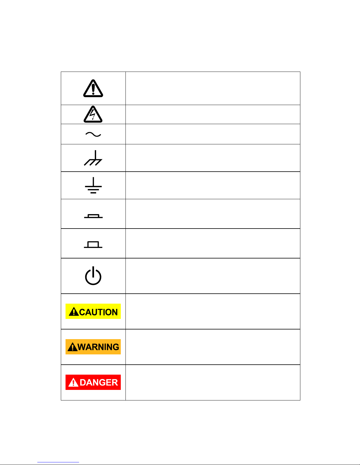
Safety Symbols

Refer to the user manual for warning information to avoid hazard or personal injury and prevent damage to instrument.

Electric Shock hazard

Alternating current (AC)

Chassis (earth ground) symbol.

Ground terminal

On (Power). This is the In position of the power switch when instrument is ON.

Off (Power). This is the Out position of the power switch when instrument is OFF.

Off (Supply). This is the AC mains connect/disconnect switch on top of the instrument.

CAUTION indicates a hazardous situation which, if not avoided, will result in minor or moderate injury

WARNING indicates a hazardous situation which, if not avoided, could result in death or serious injury

DANGER indicates a hazardous situation which, if not avoided, will result in death or serious injury.

Table of Contents

Safety Summary ........................................................................................i

Compliance Statements ........................................................................ viii

Safety Symbols ......................................................................................... x

1 General Information .........................................................................1

1.1 Product Overview ......................................................................... 1

1.2 Package Contents ......................................................................... 1

1.3 Front Panel ................................................................................... 2

Front Panel Description ........................................................................ 2

1.4 Back Panel .................................................................................... 3

Back Panel Description ......................................................................... 4

1.5 Display Information ...................................................................... 4

User Interface Description ................................................................... 5

2 Getting Started .................................................................................6

2.1 Input Power Requirements .......................................................... 6

Input Power .......................................................................................... 6

2.2 Preliminary Check ......................................................................... 6

Verify AC Input Voltage ........................................................................ 7

Connect Power ..................................................................................... 7

Self Test ................................................................................................ 7

Self Cal .................................................................................................. 7

Check Model and Firmware Version .................................................... 8

Function Check ..................................................................................... 8

Probe Safety ....................................................................................... 10

Probe Attenuation .............................................................................. 11

Probe Compensation .......................................................................... 11

3 Functions and Operating Descriptions ............................................ 13

3.1 Menu and Control Button .......................................................... 14

3.2 Connectors ................................................................................. 16

3.3 Auto Setup .................................................................................. 17

xii

3.4 Default Setup .............................................................................. 19

3.5 Universal Knob............................................................................ 20

3.6 Vertical System ........................................................................... 21

Using Vertical Position Knob and Volts/div Knob ............................... 21

3.7 Channel Function Menu ............................................................. 22

Setting up Channels ............................................................................ 25

3.8 Math Functions ........................................................................... 31

FFT Spectrum Analyzer ....................................................................... 32

3.9 Using REF .................................................................................... 39

3.10 Horizontal System....................................................................... 40

Horizontal Control Knob ..................................................................... 41

Window Zone ..................................................................................... 42

3.11 Trigger System ............................................................................ 43

Signal Source ...................................................................................... 44

Trigger Type ........................................................................................ 45

Coupling .............................................................................................. 63

Position ............................................................................................... 63

Slope and Level ................................................................................... 63

Trigger Holdoff ................................................................................... 64

3.12 Signal Acquisition System ........................................................... 65

3.13 Display System ............................................................................ 70

X-Y Format .......................................................................................... 74

3.14 Measure System ......................................................................... 75

Scale Measurement ............................................................................ 75

Cursor Measurement ......................................................................... 75

3.15 Storage System ........................................................................... 88

Recalling Files ..................................................................................... 90

Creating Folders and Files .................................................................. 90

Save/Recall Setup ............................................................................... 91

Save/Recall Waveform ....................................................................... 95

3.16 Utility System............................................................................ 102

System Status ................................................................................... 106

Language .......................................................................................... 107

Self Calibration ................................................................................. 107

Self Test ............................................................................................ 108

Update Firmware.............................................................................. 111

xiii

Pass/Fail ............................................................................................ 112

Waveform Record ............................................................................ 117

Recorder (Scan Mode Only) ............................................................. 121

Help Menu ........................................................................................ 124

4 Application Examples ................................................................... 125

4.1 Taking Simple Measurements .................................................. 125

4.2 Taking Cursor Measurements................................................... 126

4.3 Capturing a Single-Shot Signal .................................................. 128

4.4 Analyzing Signal Details ............................................................ 129

4.5 Triggering on a Video Signal ..................................................... 130

4.6 Application of X-Y Function ...................................................... 131

4.7 Analyzing a Differential Communication Signal........................ 133

5 Remote Control ............................................................................ 134

6 Message Prompts and Troubleshooting ........................................ 135

6.1 Message Prompts ..................................................................... 135

6.2 Troubleshooting ....................................................................... 136

7 Specifications ............................................................................... 138

8 Calibration .................................................................................... 142

SERVICE INFORMATION ....................................................................... 143

LIMITED ONE-YEAR WARRANTY ........................................................... 144

1 General Information

1.1 Product Overview

The B&K Precision 2190D digital storage oscilloscope (DSO) is a portable benchtop instrument used for making measurements of signals and waveforms. The oscilloscope’s bandwidth is capable of capturing up to 100 MHz signals with a real time sampling rate of up to 1 GSa/s. With up to 40k points of deep memory, it allows for capturing more details of a signal for analysis and displayed on the large color LCD display.

Features:

 2 Channels, Bandwidth: 100 MHz  Single channel real-time sampling rate of up to 1GSa/s  Up to 40k points of memory depth  7” Color TFT LCD display  Trigger types: Edge, Pulse, Video, Slope and Alternative  Unique Digital Filter function and Waveform recorder function  Auto measure 32 parameters (Voltage and Time)  Standard interface: USB Host, USB Device, RS-232, Pass/Fail Out

1.2 Package Contents

Please inspect the instrument mechanically and electrically upon receiving it. Unpack all items from the shipping carton, and check for any obvious signs of physical damage that may have occurred during transportation. Report any damage to the shipping agent immediately. Save the original packing carton for possible future reshipment. Every instrument is shipped with the following contents:

 1 x 2190D 100 MHz Digital Storage Oscilloscope  1 x User Manual (printed)  1 x AC power cord  1 x USB type A to Type B cable

 2 x 1:1/10:1 Passive Oscilloscope Probes

Verify that all items above are included in the shipping container. If anything is missing, please contact B&K Precision.

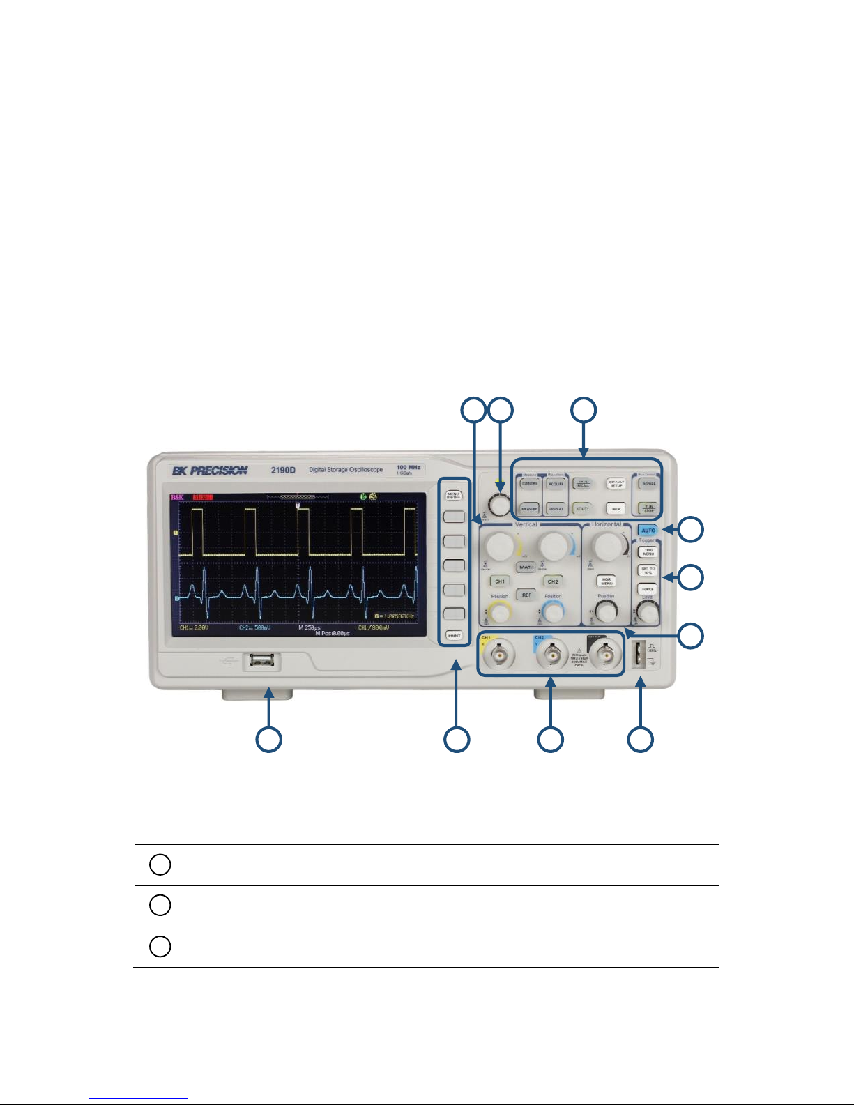
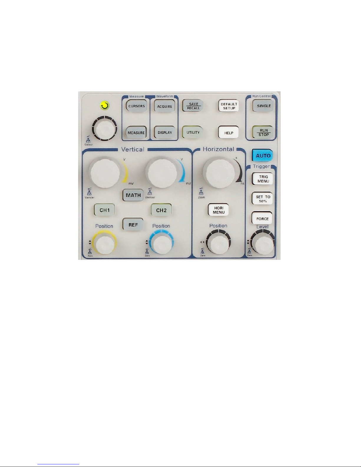
1.3 Front Panel

It is important for you to familiarize yourself with the DSO’s front panel before operating the instrument. Below is a brief introduction of the front panel function operation.

Figure 1.1 – Front Panel

Front Panel Description

Front USB (Type A) Connector

Menu function keys, Menu On/Off, Print keys

Input Channels (1 MΩ BNC)

Probe Compensator (1 kHz and Ground)

Horizontal Controls (Time Base)

Trigger Controls

Auto Function Button

Menu and Measurement Buttons

Universal Knob

Vertical Controls

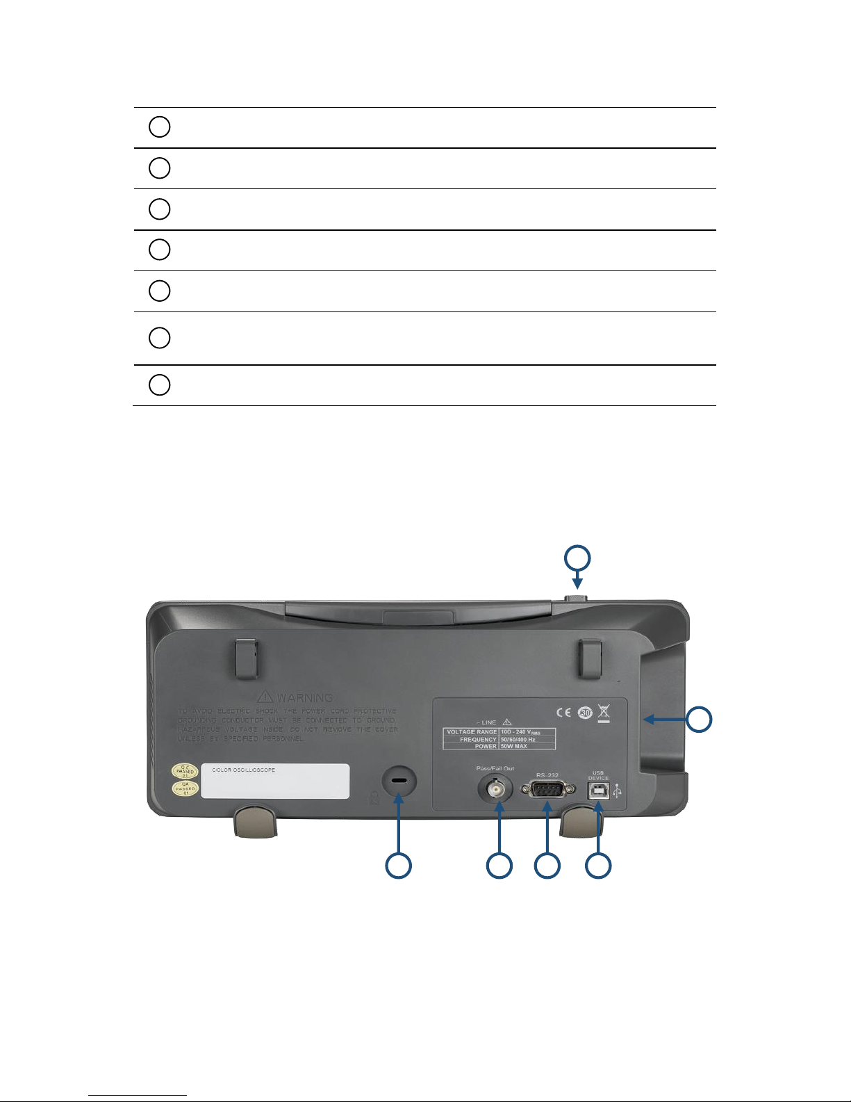
1.4 Back Panel

The following images show back and side panel connection locations.

Figure 1.2 – Back Panel

9 4 5 7 8

Back Panel Description

Security Lock Receptacle

Pass/Fail Output

RS-232 Connector

Rear USB (Type B) Device Connector

Power Input Connector

AC Power Switch

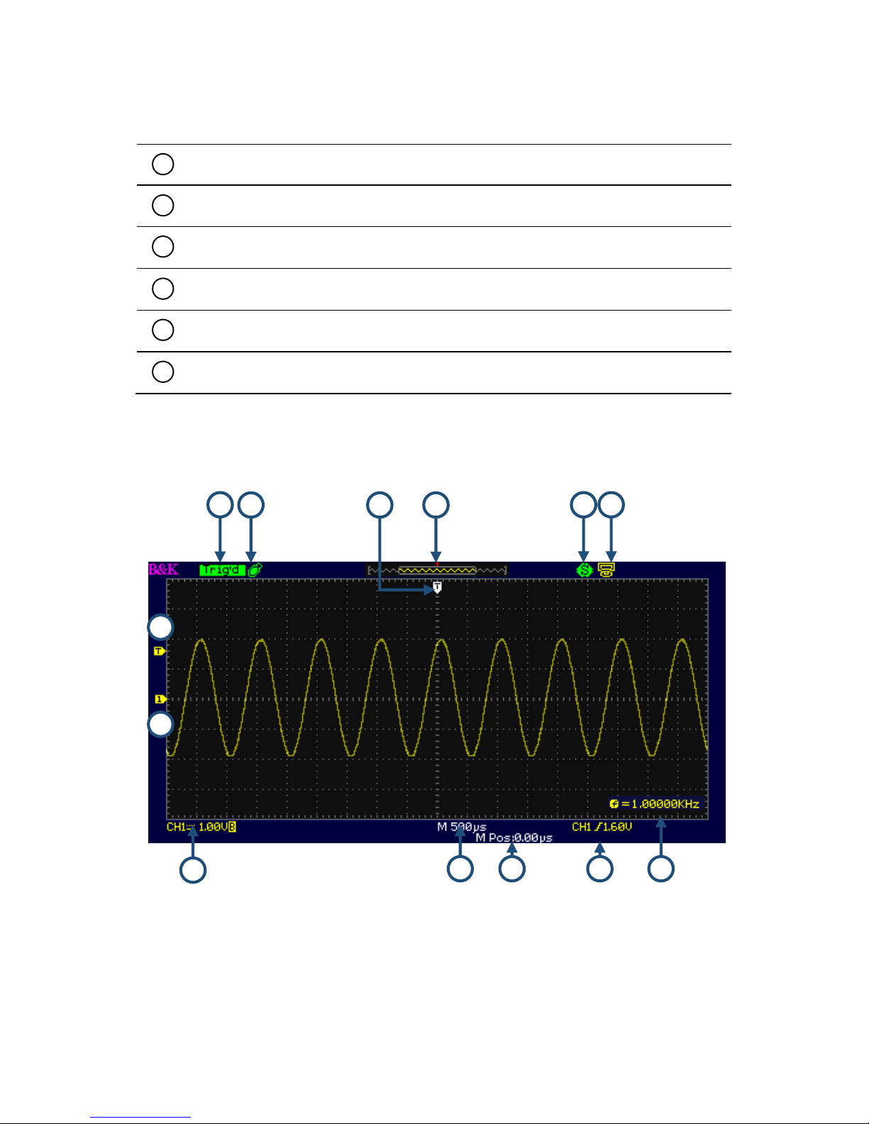
1.5 Display Information

Figure 1.3 – Display Screen

1 2 3 4 5

User Interface Description

Trigger Level Display Marker

Vertical Display Markers (Ground Reference)

Channel Source, Coupling Type, Volts/Division, BW Limit Indicator

Timebase Setting

Horizontal Trigger Position Display

Frequency Counter

Trigger Source, Type, and Level Indicator

Rear USB Indicator

Print Key Save Function Indicator

Waveform Display Preview

Horizontal Trigger Position Marker

USB Flash Drive Indicator

Trigger Status

1 2 3 4 5

2 Getting Started

Before connecting and powering up the instrument, please review and go through the instructions in this chapter.

2.1 Input Power Requirements

Input Power

The supply has a universal AC input that accepts line voltage and frequency input within:

100 – 240 V (+/- 10%), 50 /60 Hz (+/- 5%)

100 – 127 V, 45 – 440 Hz

Before connecting to an AC outlet or external power source, be sure that the power switch is in the OFF position and verify that the AC power cord, including the extension line, is compatible with the rated voltage/current and that there is sufficient circuit capacity for the power supply. Once verified, connect the cable firmly.

The included AC power cord is safety certified for this instrument operating in rated range. To change a cable or add an extension cable, be sure that it can meet the required power ratings for this instrument. Any misuse with wrong or unsafe cables will void the warranty.

2.2 Preliminary Check

Complete the following steps to verify that the oscilloscope is ready for use.

Verify AC Input Voltage

Verify and check to make sure proper AC voltages are available to power the instrument. The AC voltage range must meet the acceptable specification as explained in section 2.1.

Connect Power

Connect AC power cord to the AC receptacle in the rear panel and press the power switch to the ON position to turn ON the instrument. The instrument will have a boot screen while loading, after which the main screen will be displayed.

Self Test

The instrument has 3 self-test options to test the screen, keys, and the LED back lights of the function, menu, and channel keys as shown below.

Figure 2.1 – Self Test Menu

To perform the self test, please refer to the Self Test section for further instructions.

Self Cal

This option runs an internal self calibration procedure that will

check and adjust the instrument. To perform the self calibration, please refer to the Self Calibration section for further instructions.

Check Model and Firmware Version

The model and firmware version can be verified from within the menu system.

Press Utility and select System Status option. The software/firmware version, hardware version, model, and serial number will be displayed. Press the Single key to exit.

Function Check

Follow the steps below to do a quick check of the oscilloscope’s functionality.

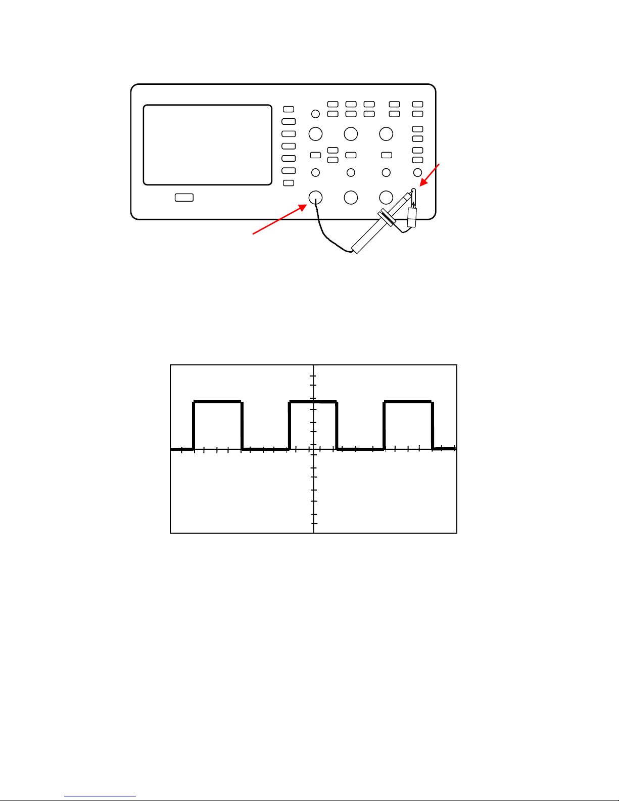
1. Power on the oscilloscope. Press “DEFAULT SETUP” to show the

result of the self check. The probe default attenuation is 1X.

Figure 2.2 – Scope Layout

2. Set the switch to 1X on the probe and connect the probe to

channel 1 on the oscilloscope. To do this, align the slot in the probe connector with the key on the CH 1 BNC, push to connect, and twist to the right to lock the probe in place. Connect the probe tip and reference lead to the PROBE COMP connectors.

Figure 2.3 – Probe Compensation

3. Press “AUTO” to show the 1 kHz frequency and about 3V peak-

peak square wave in couple seconds.

Figure 2.4 – 3 Vpp Square Wave

4. Press “CH1” two times to turn off channel 1, Press“CH2” to

change screen into channel 2, reset the channel 2 as step 2 and step 3.

PROBE

COMP

CH1

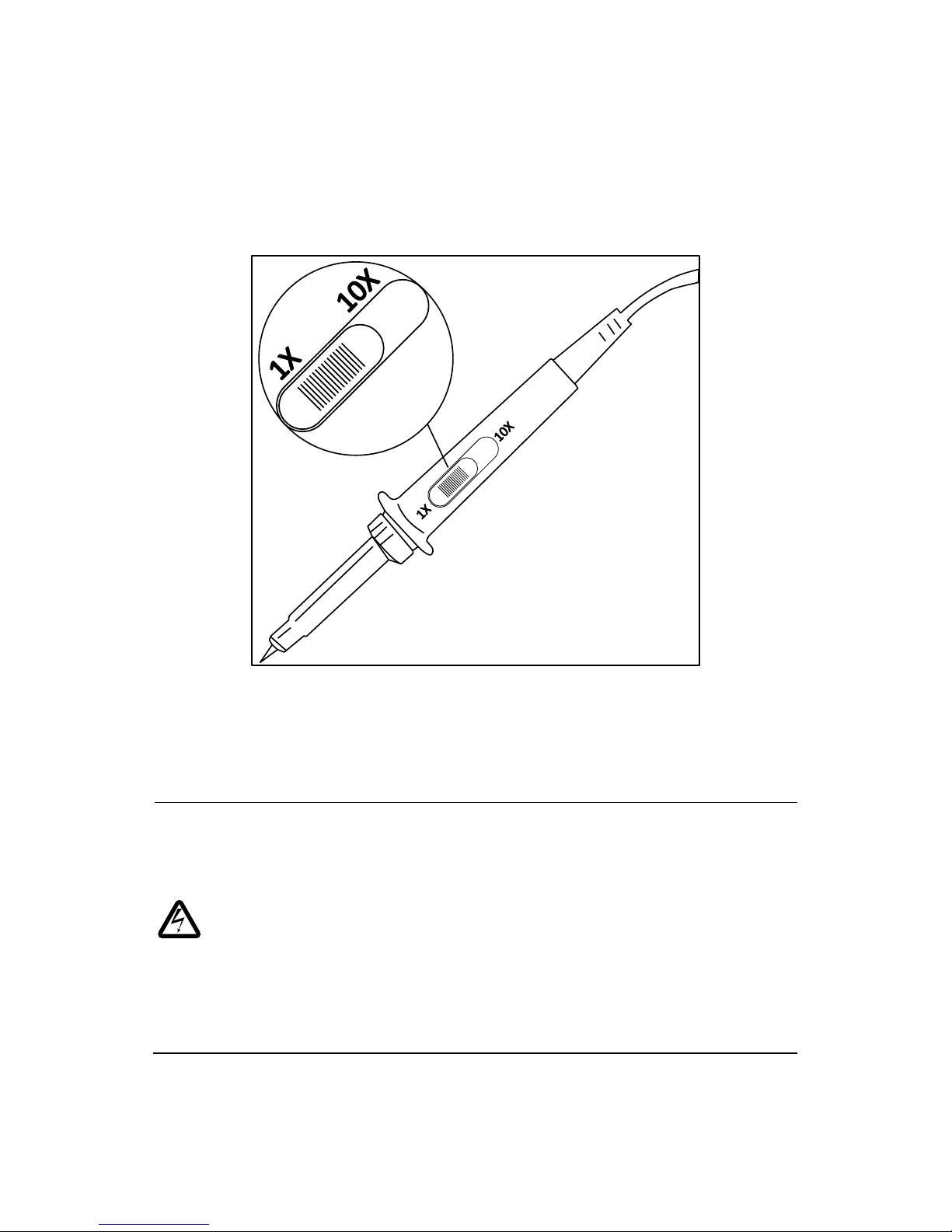
Probe Safety

A guard around the probe body provides a finger barrier for protection from electric shock.

Figure 2.5 – Oscilloscope Probe

Connect the probe to the oscilloscope and connect the ground terminal to ground before you take any measurements.

SHOCK HAZARD

To avoid electric shock when using the probe, keep fingers behind the guard on the probe body.

To avoid electric shock while using the probe, do not touch metallic portions of the probe head while it is connected to a voltage source. Connect the probe to the oscilloscope and connect the ground terminal to ground before you take any measurements.

Probe Attenuation

Probes are available with various attenuation factors which affect the vertical scale of the signal. The Probe Check function verifies that the Probe attenuation option matches the attenuation of the probe.

You can push a vertical menu button (such as the CH 1 MENU button), and select the Probe option that matches the attenuation factor of your probe.

NOTE: The default setting for the Probe option is 1X.

Be sure that the attenuation switch on the probe matches the Probe option in the oscilloscope. Switch settings are 1X and 10X.

NOTE: When the attenuation switch is set to 1X, the probe limits

the bandwidth of the oscilloscope to 6 MHz (according to Probe spec). To use the full bandwidth of the oscilloscope, be sure to set

the switch to 10X

Probe Compensation

As an alternative method to Probe Check, you can manually perform this adjustment to match your probe to the input channel.

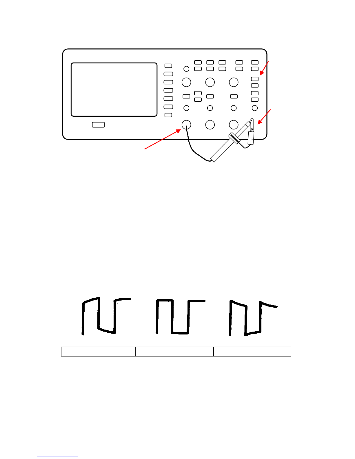
Figure 2.6 – Probe Compensation Setup

1. Set the Probe option attenuation in the channel menu to 10X. Do

so by pressing CH1 button and selecting “Probe” from menu.

Select 10X. Set the switch to 10X on the probe and connect the probe to channel 1 on the oscilloscope. If you use the probe hook-tip, ensure a proper connection by firmly inserting the tip onto the probe.

2. Attach the probe tip to the PROBE COMP 3V connector and the

reference lead to the PROBE COMP Ground connector. Display the channel and then push the “AUTO” button.

3. Check the shape of the displayed waveform.

Figure 2.7 – Compensation Illustration

4. If necessary, adjust your probe’s compensation trimmer pot.

Repeat as necessary.

AUTO BUTTO

PROBE

COMP

CH1

Overcompensated

Compensated Correctly

Undercompensated

3 Functions and Operating

Descriptions

To use your oscilloscope effectively, you need to learn about the following oscilloscope functions:

• Menu and control button

• Connector

• Auto Setup

• Default Setup

• Universal knob

• Vertical System

• Channel Function Menu

• Math Functions

• Using REF

• Horizontal System

• Trigger System

• Acquiring signals System

• Display System

• Measuring waveforms System

• Utility System

• Storage System

• Online Help function

3.1 Menu and Control Button

Figure 3.1 – Control Buttons

 Channel buttons (CH1, CH2): Press a channel button to turn

that channel ON or OFF and open the channel menu for that channel. You can use the channel menu to set up a channel. When the channel is on, the channel button is lit.

 MATH: Press to display the Math menu. You can use the

MATH menu to use the oscilloscope’s Math functions.

 REF: Press to display the Ref Wave menu. You can use this

menu to save and recall four or two reference waveforms to and from internal memory.

 HORI MENU: Press to display the Horizontal menu. You can

use the Horizontal menu to display the waveform and zoom in a segment of a waveform.

 TRIG MENU: Press to display the Trigger menu. You can use

the Trigger menu to set the trigger type (Edge. Pulse, Video, Slope, Alternative) and trigger settings.

 SET TO 50%: Press to stabilize a waveform quickly. The

oscilloscope can set the trigger level to be halfway between the minimum and maximum voltage level automatically. This is useful when you connect a signal to the EXT TRIG connector and set the trigger source to Ext or Ext/5.

 FORCE: Use the FORCE button to complete the current

waveform acquisition whether the oscilloscope detects a trigger or not. This is useful for Single acquisitions and Normal trigger mode.

 SAVE/RECALL: Press to display the Save/Recall menu. You

can use the Save/Recall menu to save and recall up to 20 oscilloscope setups and 10 waveforms to/from internal memory or a USB memory device (limited by memory capacity of the USB flash drive). You can also use it to recall the default factory settings, to save waveform data as a comma-delimited file (.CSV), and to save the displayed waveform image.

 ACQUIRE: Press to display Acquire menu. You can use the

Acquire menu to set the acquisition Sampling Mode (Sampling, Peak Detect, and Average).

 MEASURE: Press to display a menu of measurement

parameters.

 CURSORS: Display the Cursor Menu. Vertical Position

controls adjust cursor position while displaying the Cursor Menu and the cursors are activated. Cursors remain

displayed (unless the “Type” option is set to “Off”) after

leaving the Cursor Menu but are not adjustable.

 DISPLAY: Press to open the Display menu. You can use the

Display menu to set grid and waveform display styles, and persistence.

 UTILITY: Press to open the Utility menu. You can use the

Utility menu to configure oscilloscope features, such as

sound, language, counter, etc. You can also view system status and update software.

 DEFAULT SETUP: Press to reset the oscilloscope’s settings to

the default factory configuration.

 HELP: Enter the online help system.  AUTO: Automatically sets the oscilloscope controls to

produce a usable display of the input signals.

 RUN/STOP: Continuously acquires waveforms or stops the

acquisition.

 Note: If waveform acquisition is stopped (using the

RUN/STOP or SINGLE button), the TIME/DIV control expands or compresses the waveform.

 SINGLE: Acquire a single waveform and then stops waveform

acquisition.

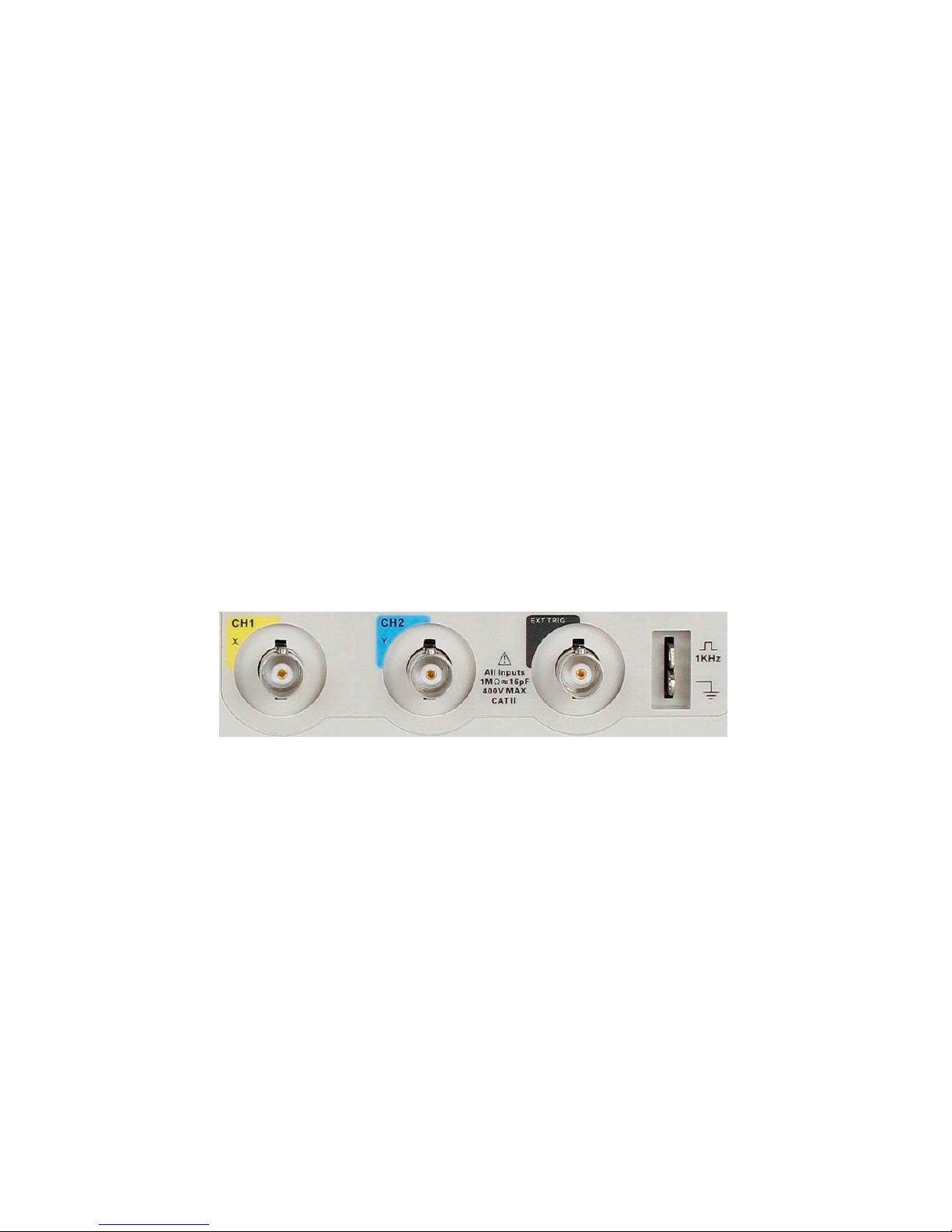
3.2 Connectors

Figure 3.2 – Connectors

 Channel Connector (CH1, CH2): Input connectors for waveform

display.

 EXT TRIG: Input connector for an external trigger source. Use the

Trigger Menu to select the “Ext” or “Ext/5” trigger source.

 Probe Compensation: 1 kHz voltage probe compensation output

and ground. Use to electrically match the probe to the oscilloscope input circuit.

3.3 Auto Setup

The 2190D Digital Storage Oscilloscope has an Auto Setup function that identifies the waveform types and automatically adjusts controls to produce a usable display of the input signal.

Press the AUTO front panel button, and then press the menu option button adjacent to the desired waveform as follows:

Figure 3.3 – Auto Setup

Table 3.1 – Autoset Menu

Option

Description

(Multi-cycle sine)

Auto set the screen and display several cycles signal.

(Single-cycle sine)

Set the screen and auto display single cycle signal.

(Rising edge)

Auto set and show the rising time.

(Falling edge)

Auto set and show the falling time.

(Undo Setup)

Causes the oscilloscope to recall the previous setup.

Auto Set determines the trigger source based on the following conditions:

• If multiple channels have signals, channel with the lowest

frequency signal.

• No signals found, the lowest-numbered channel displayed when

Auto set was invoked.

• No signals found and no channels displayed, oscilloscope displays

and uses channel 1.

Table 3.2 – Auto Set Function Menu Items

Function

Setting

Acquire Mode

Adjusted to Sampling

Display Format

Y-T

Display Type

Set to Dots for a video signal, set to Vectors for an FFT spectrum; otherwise, unchanged

Vertical Coupling

Adjusted to DC or AC according to the input signal

Bandwidth Limit

Off(full)

V/div

Adjusted

VOLTS/DIV adjustability

Coarse

Signal inverted

Off

Horizontal position

Center

Time/div

Adjusted

Trigger type

Edge

Trigger source

Auto detect the channel which has the input signal

Trigger slope

Rising

Trigger mode

Auto

Trigger coupling

Trigger holdoff

Minimum

Trigger level

Set to 50%

NOTE: The AUTO button can be disabled. Please see “Appendix C Disabling Auto Function” for details.

3.4 Default Setup

The oscilloscope is set up for normal operation when it is shipped from the factory. This is the default setup. To recall this setup, press the DEFAULT SETUP button. For the default options, buttons and controls when you press the DEFAULT SETUP button, refer to “Appendix A Default Setup”.

The DEFAULT SETUP button does not reset the following settings:

• Language option

• Saved reference waveform files

• Saved setup files

• Display contrast

• Calibration data

3.5 Universal Knob

Figure 3.4 – Universal Knob

You can use the Universal knob with many functions, such as adjusting the hold off time, moving cursors, setting the pulse width, setting the video line, adjusting the upper and lower frequency limit, adjusting the X and Y masks when using the pass/fail function, etc. You can also turn the

“Universal” knob to adjust the storage position of setups, waveforms,

pictures when saving/recalling, and to select menu options. With some functions, the light indicator above the knob will turn on to indicate that the knob can be used to make changes or adjustments for that function. The knob can also be pushed to make a selection after changes/adjustments have been made.

3.6 Vertical System

The vertical control could be used for displaying waveform, rectify scale and position.

Figure 3.5 – Vertical System Controls

Using Vertical Position Knob and Volts/div Knob

• Vertical “POSITION” Knob

1. Use the Vertical “POSITION” knobs to move the channel

waveforms up or down on the screen. This button’s

resolution varies as per the vertical scale.

2. When you adjust the vertical position of channels

waveforms, the vertical position information will display on the bottom left of the screen. For example “Volts Pos=24.6mV”.

3. Press the vertical “POSITION” knob to set the vertical

position to zero.

• “Volts/div” Knob

1. Use the “Volts/div” knobs to control how the

oscilloscope amplifies or attenuates the source signal of

channel waveforms. When you turn the “volts/div”

knob, the oscilloscope increases or decreases the vertical size of the waveform on the screen with respect to the ground level.

2. When you press the “Volt/div” knob, you can switch

“Volts/div” option between “Coarse” and “Fine”. The vertical scale is set by a 1-2-5 step sequence in Coarse mode. Increase in the clockwise direction and decrease in the counterclockwise direction. In Fine mode, the knob changes the Volts/Div scale in small steps between the coarse settings. Again, increase in the clockwise direction and decrease in the counterclockwise direction.

3.7 Channel Function Menu

Table 3.3 – Channel Function Menu

Option

Setting

Introduction

Coupling

GND

DC passes both AC and DC components of the input signal.

AC blocks the DC component of the input signal and attenuates signals below 10 Hz.

GND disconnects the input signal.

BW limit

Off

Limits the bandwidth to reduce display noise; filters the signal to reduce noise and other unwanted high frequency components.

Volts/Div

Coarse

Fine

Selects the resolution of the Volts/Div knob

Coarse defines a 1-2-5 sequence.

23 Fine changes the resolution to small steps between the coarse settings.

Probe

1X, 5X 10X, 50X 100X, 500X, 1000X

Set to match the type of probe you are using to ensure correct vertical readouts.

Page 1/3

Press this button to enter the second page menu

Table 3.4 – Channel Function Menu 2

Option

Setting

Instruction

Invert

off

Turn on invert function.

Turn off invert function.

Filter

Press this button to enter the “Digital Filter menu”.

Page 2/3

Press this button to enter the third page menu.

Table 3.5 – Channel Function Menu 3

Option

Setting

Introduction

Unit

V A Set the scale unit to voltage

Set the scale unit to current.

Skew

-100 ns – 100ns

Set the skew time between two channels.

Page 3/3

Press this button to return to the first page menu.

Table 3.6 – Digital Filter Menu

Option

Setting

Introduction

Digital Filter

Off

Turn on the digital filter.

Turn off the digital filter.

Type

Setup as LPF (Low Pass Filter).

Setup as HPF (High Pass Filter).

Setup as BPF (Band Pass Filter).

Setup as BRF (Band Reject Filter).

Upper_limit

Turn the “Universal” knob to set

upper limit.

Lower_limit

Turn the “Universal” knob to set

lower limit.

Return

Return to the second page menu.

• “GND” Coupling: Use GND coupling to display a zero-volt

waveform. Internally, the channel input is connected to a zerovolt reference level.

• Fine Resolution: The vertical scale readout displays the actual

Volts/Div setting while in the fine resolution setting. Changing the setting to coarse does not change the vertical scale until the VOLTS/DIV control is adjusted.

NOTE:

The oscilloscope’s vertical response rolls off slowly above its specified bandwidth. Therefore, the FFT spectrum can show valid frequency information higher than the oscilloscope’s bandwidth. However, the magnitude information near or above the

bandwidth will not be accurate.

If the channel is set to DC coupling, you can quickly measure the DC component of the signal by simply noting its distance from the ground symbol.

If the channel is set to AC coupling, the DC component of the signal is blocked allowing you to use greater sensitivity to display the AC component of the signal.

Setting up Channels

Each channel has its own separate Menu. The items are set up separately according to each channel.

1. Setup Channel Coupling

Take CH1 for example; the tested signal is a sine wave signal with DC deflection:

• Press “CH1”→“Coupling”→“AC”, Set to AC couple mode.

This will block the DC component of the input signal.

Figure 3.6 – AC Coupling

• Press “CH1”→“Coupling”→“DC”, Set to DC couple mode.

Both DC and AC components of the input signal will be captured.

Figure 3.7 – DC Coupling

• Press “CH1”→“Coupling”→“GND”, Set to GROUND mode.

This disconnects the input signal.

Figure 3.8 – Ground Coupling

2. Bandwidth Limiting

Take CH1 for example:

• Press “CH1”→“BW Limit”→ “On”, and bandwidth will be

limited to 20 MHz.

• Press “CH1”→“BW Limit”→ “Off”, and bandwidth limit

will be disabled.

Figure 3.9 – Bandwidth Limit

3. Volts/Div Settings

Vertical scale adjust have Coarse and Fine modes, Vertical sensitivity range of 2 mV/div – 10 V/div. Take CH1 for example:

• Press “CH1”→“Volts/Div”→“Coarse”. It is the default

setting of Volts/Div, and makes the vertical scaling in a 12-5-step sequence from 2 mV/div, 5 mV/div, 10 mV/div to 10 V/div.

• Press “CH1”→ Volts/Div”→ Fine”. This setting changes

the vertical control to small steps between the coarse settings. It will be helpful when you need to adjust the waveform vertical size in smaller steps.

Figure 3.10 – Coarse/Fine Control

4. Setting Probe Attenuation

In order to set the attenuation coefficient, you need to specify it in the channel operation Menu. If the attenuation coefficient is 10:1, the input coefficient should be set to 10X, so that the Volts/div information and measurement testing is correct. Take CH1 for example, when you use the 100:1 probe:

• Press “CH1”→“Probe” →“100X”

Figure 3.11 – Probe Attenuation Setting

5. Inverting Waveforms

Take CH1 for example:

• Press “CH1”→ Next Page “Page 1/3” →“Invert”→“On”:

Figure 3.12 – Invert Waveform Screen

6. Using the Digital Filter

• Press “CH1”→ Next Page “Page 1/3”→ “Filter”, display

the digital filter menu. Select “Filter Type”, then select “Upper Limit” or “Lower Limit” and turn the “Universal”

knob to adjust them.

• Press “CH1”→ Next Page “Page 1/3”→ “Filter” →“Off”.

Turn off the Digital Filter function.

Figure 3.13 – Digital Filter Menu

• Press “CH1”→ “Next Page “Page 1/3”→ “Filter” → “On”.

Turn on the Digital Filter function.

Figure 3.14 – Digital Filter Adjustment Screen

3.8 Math Functions

Math shows the results after +,-,*, / and FFT operations of the CH1 and CH2. Press the MATH button to display the waveform math operations. Press the MATH button again to remove the math waveform display.

Table 3.7 – Math Function Menu

Function

Setting

Description

Operation

+, -, *, /, FFT

Math operates between signal source CH1 and CH2.

Source A

CH1 – CH2

Select CH1 or CH2 as Source A.

Source B

CH1 – CH2

Select CH1 or CH2 as Source B.

Invert

off

Invert the MATH waveform.

Turn off MATH Invert function.

Page 1/2

Enter the second page of MATH menu.

Table 3.8 – Math Function Menu 2

Function

Setting

Description

Use universal knob to adjust the vertical position of the MATH waveform.

Use universal knob to adjust the vertical scale of the MATH waveform.

Page 2/2

Go back to first page of MATH menu.

Table 3.9 – Math Function Description

Operation

Setting

Description

＋

A+B

Source A waveform adds Source B waveform.

－

A-B

Source B waveform is subtracted from Source A waveform.

A*B

Source A multiplied by Source B

A/B

Source A divided by Source B

FFT

Fast Fourier Transform.

Figure 3.15 – Math Waveform

FFT Spectrum Analyzer

The FFT process mathematically converts a time-domain signal into its frequency components. You can use the Math FFT mode to view the following types of signals:

• Analyze the harmonic wave in the Power cable.

• Test the harmonic content and distortion in the system

• Show the Noise in the DC Power supply

• Test the filter and pulse response in the system

• Analyze vibration

Table 3.10 – FFT Function Menu 1

FFT Option

Setting

Description

Source

CH1, CH2

Select this channel as the FFT source.

Window

Hanning

Hamming

Rectangular

Blackman

Select FFT window types.

FFT ZOOM

10X

Changes the horizontal magnification of the FFT display.

Page 1/2

Enter the second page of FFT menu.

Table 3.11 – FFT Function Menu 2

FFT Option

Setting

Description

Scale

Vrms

Set Vrms to be the Vertical Scale unit.

dBVrms

Set dBVrms to be the vertical

Scale unit.

Display

Split

Full screen

Display FFT waveform on half screen.

Display FFT waveform on full screen.

Page 2/2

Return to the first page of FFT menu.

To use the Math FFT mode, you need to perform the following steps:

1. Set up the source (time-domain) waveform.

2. Press the AUTO button to display an YT waveform.

3. Turn the vertical “POSITION” knob to move the YT waveform to

the center vertically (zero divisions).

4. Turn the horizontal “POSITION” knob to position the part of the

YT waveform that you want to analyze in the center eight divisions of the screen. The oscilloscope calculates the FFT spectrum using the center 1024 points of the time-domain waveform.

5. Turn the “Volts/div” knob to ensure that the entire waveform

remains on the screen.

6. Turn the “S/div” knob to provide the resolution you want in the

FFT spectrum.

7. If possible, set the oscilloscope to display many signal cycles.

To display FFT correctly, follow these steps:

1. Push the “MATH” button.

2. Set the “Operation” option to FFT.

3. Press the “Source” button to select “CH1” or “CH2” according to

input signal channel.

4. Turn the “Time/div” knob to adjust the sampling rate (this

parameter is displayed behind the time base parameter), making sure it is at least double the input signal frequency. (to avoid aliasing according to Nyquist’s theorem)

Displaying the FFT Spectrum

Press the MATH button to display the Math Menu. Use the options to select the Source channel, Window algorithm, and FFT Zoom factor. You

can display only one FFT spectrum at a time. You can select “Full screen” or “Split” in “Display” option to display FFT waveform on full screen or

display channel waveform and its FFT waveform on half screen at a time.

Select FFT window

Windows reduce spectral leakage in the FFT spectrum. The FFT assumes that the YT waveform repeats forever. With an integral number of cycles, the YT waveform starts and ends at the me amplitude and there are no discontinuities in the signal shape A non-integral number of cycles in the YT waveform causes the signal start and end points to be at different amplitudes. The transitions between the start and end points cause discontinuities in the signal that introduce high-frequency transients.

Table 3.12 – FFT Window Description

Window

Characteristics

Applications

Rectangular

Best frequency resolution, worst magnitude resolution. This is essentially the

Symmetric transients or bursts. Equalamplitude sine waves with fixed frequencies.

same as no window.

Broadband random noise with a relatively slowly varying spectrum.

Hanning Hamming

Better frequency, poorer magnitude accuracy than Rectangular. Hamming has slightly better frequency resolution than Hanning.

Sine, periodic, and narrow-band random noise. Asymmetric transients or bursts.

Blackman

Best magnitude, worst frequency resolution.

Single frequency waveforms, to find higher order harmonics.

Magnifying the FFT Spectrum

You can magnify and use cursors to take measurements on the FFT

spectrum. The oscilloscope includes an “FFT Zoom” option to magnify horizontally, press this option button to select “1X”, “2X”, “5X” or “10X”. Moreover, you also can turn the “Universal” knob to magnify FFT

waveform horizontally in a 1-2-5 step. To magnify vertically, turn the “Volts/div” knob.

Measuring an FFT Spectrum Using Cursors

You can take two measurements on FFT spectrums: magnitude (in dB) and frequency (in Hz). Magnitude is referenced to 0 dB, where 0 dB equals 1 VRMS. You can use the cursors to take measurements at any zoom factor. Use horizontal cursors to measure amplitude and vertical cursors to measure frequency.

If you input a sine signal into channel 1, follow these steps:

• Measure FFT Amplitude

1. Input a sine signal to channel 1, and press the

“AUTO” button.

2. Press the “MATH” button to enter the “MATH”

menu.

3. Press the “Operation” option button to select “FFT”.

4. Press the “Source” option button to select “CH1”.

5. Press CH1 button to display CH1 menu.

6. Turn the “Time/div” knob to adjust the sampling

rate (at least double the frequency of input signal).

7. If FFT is displayed on full screen, press CH1 button

again to remove channel waveform display.

8. Press the “CURSOR” button to enter “Cursor” menu.

9. Press the “Cursor Mode” button to select “Manual”.

10. Press the “Type” option button to select “Voltage”.

11. Press the “Source” option button to select “MATH”.

12. Press the “CurA” option button; turn the “Universal”

knob to move Cursor A to the highest point of the FFT waveform.

13. Press the “CurB” option button, turn the “Universal”

knob to move Cursor B to the lowest point of the FFT waveform.

14. The amplitude (△T) displays on the top of the left

screen.

Figure 3.16 – Measuring FFT Amplitude

• Measure FFT Frequency

1. Press the CURSOR button.

2. Press the “Cursor Mode” button to select “Manual”.

3. Press the “Type” option button to select “Time”.

4. Press the “Source” option button to select “MATH”.

5. Press the “CurA” option button, turn the “Universal”

button to move Cursor A to the highest position of the FFT waveform.

6. The value of CurA displaying on the top of the left

screen is FFT frequency. This frequency should be the same as input signal frequency.

Figure 3.17 – Measuring FFT Frequency

NOTE:

The FFT of a waveform that has a DC component or offset can cause incorrect FFT waveform magnitude values. To minimize the DC component, choose AC Coupling on the source waveform.

To display FFT waveforms with a large dynamic range, use the dBVrms scale. The dBVrms scale displays component magnitudes using a log scale.

The Nyquist frequency is the highest frequency that any real-time digitizing oscilloscope can acquire without aliasing. This frequency is half that of the sample rate provided it is within the analog bandwidth of the oscilloscope. Frequencies above the Nyquist frequency will be undersampled, which causes aliasing.

3.9 Using REF

The reference control saves waveforms to a nonvolatile waveform memory. The reference function becomes available after a waveform has been saved.

Table 3.13 – REF Function Menu

Option

Setting

Description

Source

CH1,CH2,

CH1 off

CH2 off

Choose the waveform display to store.

REFA

REFB

Choose the reference location to store or recall a waveform.

Save

Stores source waveform to the chosen reference location.

REFA

REFB

off

Recall the reference waveform on the screen.

Turn off the reference waveform.

Press the Ref button to display the “Reference waveform menu”.

Figure 3.18 – Reference Waveform Menu

Operation step:

1. Press the “REF” menu button to display the “Reference waveform

menu”.

2. Press the “Source” option button to select input signal channel.

3. Turn the vertical “POSITION” knob and “Volts/div” knob to adjust

the vertical position and scale.

4. Press the third option button to select “REFA” or “REFB” as

storage position.

5. Press the “Save” option button.

6. Press the bottom option button to select “REFA On” or “REFB On”

to recall the reference waveform.

NOTE:

X-Y mode waveforms are not stored as reference waveforms.

You cannot adjust the horizontal position and scale of the reference waveform.

3.10 Horizontal System

Shown below are two knobs and one button in the HORIZONTAL area.

Figure 3.19 – Horizontal Controls

Table 3.14 – Horizontal System Function Menu

Option

Setting

Description

Delayed

Off

Turn on this function for main timebase waveform to display on the top half screen and window timebase waveform to display on the below half screen at the same time.

Turn off this function to only display main timebase waveform on the screen.

Horizontal Control Knob

You can use the horizontal controls to change the horizontal scale and position of waveforms. The horizontal position readout shows the time represented by the center of the screen, using the time of the trigger as zero. Changing the horizontal scale causes the waveform to expand or contract around the screen center.

• Horizontal “POSITION” knob

1. Adjust the horizontal position of all channels and

math waveforms (the position of the trigger relative

to the center of the screen). The resolution of this control varies with the time base setting.

2. When you press the horizontal “POSITION” Knob,

you can set the horizontal position to zero.

• “Time/div” knob

1. Used to change the horizontal time scale to magnify

or compress the waveform. If waveform acquisition is stopped (using the RUN/STOP or SINGLE button), turn the Time/div knob to expand or compress the waveform.

2. Select the horizontal Time/div (scale factor) for the

main or the window time base. When Window Zone is enabled, it changes the width of the window zone by changing the window time base.

• Display scan mode

When the Time/div control is set to 100 ms/div or slower and the trigger mode is set to Auto, the oscilloscope enters the scan acquisition mode. In this mode, the waveform display updates from left to right. There is no trigger or horizontal position control of waveforms during scan mode.

Window Zone

Use the Window Zone option to define a segment of a waveform to see more detail. This function behaves like zooming into a portion of the captured waveform. The window time base setting cannot be set slower than the Main time base setting.

You can turn the Horizontal Position and Time/div controls to enlarge or minimize waveforms in the Window Zone.

If you want to see a section of the waveform in details, follow these steps:

1. Press the “HORI MENU” button to enter the “Horizontal menu”.

2. Turn the “Time/div” knob to change the main timebase scale.

3. Press the “Delayed” option button to select “On”.

Figure 3.20 – Horizontal Delay Menu

4. Turn the “Horizontal Position” knob (adjust window’s position) to

select the window that your need and expanded window waveform display on the below half screen at the same time.

3.11 Trigger System

The trigger determines when the oscilloscope starts to acquire data and display a waveform. When a trigger is set up properly, the oscilloscope converts unstable displays or blank screens into meaningful waveforms.

Here are three buttons and one knob in the trigger area. See below:

Figure 3.21 – Trigger Controls

• “TRIG MENU” Button: Press the “TRIG MENU” Button to

display the “Trigger Menu”.

• “LEVEL” Knob: The LEVEL knob is to set the

corresponding signal voltage of trigger point in order to

sample. Press the “LEVEL” knob to set trigger level to

zero.

• “SET TO 50%” Button: Use the “SET TO 50%” button to

stabilize a waveform quickly. The oscilloscope can set the Trigger Level to be about halfway between the minimum and maximum voltage levels automatically. This is useful when you connect a signal to the EXT TRIG BNC and set the trigger source to Ext or Ext/5.

• “FORCE Button: Use the FORCE button to complete the

current waveform acquisition whether the oscilloscope detects a trigger or not. This is useful for SINGLE acquisitions and Normal trigger mode.

Signal Source

You can use the Trigger Source options to select the signal that the oscilloscope uses as a trigger. The source can be any signal connected to a channel BNC, to the EXT TRIG BUS, or the AC power line (available only with Edge Trigger).

Trigger Type

The scopes have five trigger types: Edge, Video, Pulse, Slope, and Alternate.

Edge Trigger

Use Edge triggering to trigger on the edge of the oscilloscope input signal at the trigger threshold.

Table 3.15 – Edge Trigger Function Menu

Option

Setting

Description

Type

Edge

With Edge highlighted, the rising or falling edge of the input signal is used for the trigger.

Source

CH1

CH2

Triggers on a channel whether or not the waveform is displayed.

EXT

Does not display the trigger signal; the Ext option uses the signal connected to the EXT TRIG front-panel BNC and allows a trigger level range of -1.2V to +1.2V.

EXT/5

Same as Ext option, but attenuates the signal by a factor of five, and allows a trigger level range of +6V to -6V.This extends the trigger level range.

AC Line

This selection uses a signal derived from the power line as the trigger source; trigger coupling is set to DC and the trigger level to 0 volts.

Slope

Trigger on Rising edge of the trigger signal.

Trigger on Falling edge of the trigger signal.

Trigger on Rising edge and Falling edge of the trigger signal.

Mode

Auto

Use this mode to let the acquisition free-run in the absence of a valid trigger; This mode allows an untriggered, scanning waveform at 100 ms/div or slower time base settings.

Normal

Use this mode when you want to see only valid triggered waveforms; when you use this mode, the oscilloscope does not display a waveform until after the first trigger.

Single

When you want the oscilloscope to acquire a single waveform, press the “SINGLE” button.

Set up

Enter the “Trigger Setup Menu” (See Table 3.16).

Table 3.16 – Trigger Setup Function Menu

Option

Setting

Explain

Coupling

Passes all components of the signal

Blocks DC components, attenuates signals below 50 Hz.

HF Reject

Attenuates the high-frequency components above 150 kHz.

LF Reject

Blocks the DC component, attenuates the low-frequency components below 7 kHz.

Holdoff

Using the “universal” knob to adjust

holdoff time (sec), the holdoff value is displayed.

Holdoff

Reset

Reset holdoff time to 100ns.

47 Return

Return to the first page of “Trigger main menu”.

Figure 3.22 – Trigger Menu Screen

Operating Instructions:

1. Setup Type

 Press the “TRIG MENU” button to display “Trigger” menu.  Press the “Type” option button to select “Edge”.

2. Set up Source

 According to the input signal, press the “Source” option

button to select “CH1”, “CH2”, “EXT”, “EXT/5” or “AC Line”.

3. Set up Slope

 Press the “Slope” option button to select “ ”, “

” or “ ”.

4. Set up Trigger mode

 Press the “Trigger mode” option button to select “Auto”,

“Normal”, “Single”.

Auto: The waveform refreshes at a high speed whether the trigger condition is satisfied or not.

Normal: The waveform refreshes when the trigger condition is satisfied and waits for next trigger event occurring when the trigger condition is not satisfied.

Single: The oscilloscope acquires a waveform when the trigger condition is satisfied and then stops

5. Set up Trigger coupling

 Press the “Set Up” button to enter the “Trigger Setup

Menu”.

 Press the “Coupling” option button to select “DC”, “AC”,

“HF Reject” or “LF Reject”.

Pulse Trigger

Use Pulse Width triggering to trigger on aberrant pulses.

Table 3.17 – Pulse Trigger Function Menu 1

Option

Setting

Description

Type

Pulse

Select the pulse to trigger the pulse match the trigger condition.

Source

CH1 CH2 EXT EXT/5 AC Line

Select input signal source.

When

(Positive pulse width less

than pulse width setting)

(Positive pulse width larger

than pulse width setting)

(Positive pulse width equal

to pulse width setting)

(Negative pulse width less

than pulse width setting)

(Negative pulse width

larger than pulse width setting)

(Negative pulse width

equal to pulse width setting)

Select how to compare the trigger pulse relative to the value selected in the Set Pulse Width option.

Set Width

20.0ns～10.0s

Selecting this option can turn the universal to set up the pulse width.

Page 1/2

Press this button to enter the second page.

Figure 3.23 – Pulse Trigger Menu 1

Table 3.18 – Pulse Trigger Function Menu 2

Option

Setting

Description

Type

Pulse

Select the pulse to trigger the pulse match the trigger condition.

Mode

Auto Normal single

Select the type of triggering; Normal mode is best for most Pulse Width trigger applications.

Set up

Enter the “Trigger setup menu”.

Page 2/2

Press this button to return to the first page.

Figure 3.24 – Pulse Trigger Menu 2

Operating Instructions:

1. Setup Type

 Press the “TRIG MENU” button to display “Trigger” menu.  Press the “Type” option button to select “Pulse”.

2. Set up condition

 Press the “When” option button to select “ ”, “

”, “ ”, “ ”, “ ”or“ ”.

3. Set up pulse width

 Turn the “Universal” knob to set up width.

Video Trigger

Trigger on fields or lines of standard video signals.

Table 3.19 – Video Trigger Function Menu 1

Option

Setting

Description

Type

Video

When you select the video type, put the couple set to the AC, then you could trigger the NTSC,PAL and SECAM video signal.

Source CH1 CH2

Select the input source to be the trigger signal.

EXT EXT/5

Ext and Ext/5 use the signal applied to the EXT TRIG connector as the source.

Polarity

(Normal)

Normal triggers on the negative edge of the sync pulse.

(Inverted)

Inverted triggers on the positive edge of the sync pulse.

Sync

Line Num All lines Odd field Even Field

Select appropriate video sync.

Page 1/2

Enter the second page of “Video trigger menu”.

Table 3.20 - Video Trigger Function Menu 2

Option

Setting

Description

Type

Video

When you select the video type, put the couple set to the

52 AC, then you could trigger the

NTSC, PAL and SECAM video signal.

Standard

NTSC Pal/Secam

Select the video standard for sync and line number count.

Mode

Auto

Use this mode to let the acquisition free-run in the absence of a valid trigger; This mode allows an untriggered, scanning waveform at 100 ms/div or slower time base settings.

Normal

Use this mode when you want to see only valid triggered waveforms; when you use this mode, the oscilloscope does not display a waveform until after the first trigger.

Single

When you want the oscilloscope to acquire a single waveform, press the “SINGLE” button.

Set up

Enter the “Trigger setup menu”.

Page 2/2

Return to the first page of “Video Trigger menu”.

Figure 3.25 – Video Trigger Menu

Operating Instructions:

1. Set up Type

 Press the “TRIG MENU” button to display “Trigger” menu.  Press the “Type” option button to select “Video”.

2. Set up Polarity

 Press the “Polarity” option button to select “ ” or “

”.

3. Set up Synchronization

 Press the “Sync” option button to select “All Lines”, “Line

Num”, “Odd Field”, and “Even Field”.

 If you select “Line Num”, you can turn the “Universal”

knob to set the appointed line number.

4. Set up Standard

 Press the “Next Page - Page 2/2” option  Press the “Standard” option button to select

“PAL/SECAM” or “NTSC”.

Slope Trigger

Trigger on positive slope or negative slope of waveform, according to setup time of the oscilloscope.

Table 3.21 – Slope Trigger Function Menu 1

Option

Setting

Instruction

Type

Slope

Trigger on positive slope of negative slope according to setup time of the oscilloscope.

Source

CH1

CH2

EXT

EXT/5

Select trigger source. When

Select trigger condition.

Time <Set time>

Turn the “Universal” knob to set

slope time. Time setup range is 20ns-10s.

Page 1/2

Enter the second page of slope trigger.

Figure 3.26 – Slope Trigger Menu 1

Table 3.22 – Slope Trigger Function Menu 2

Option

Setting

Instruction

Type

Slope

Trigger on positive slope or negative slope according to setup time of the oscilloscope.

Vertical

Select the trigger level that can be

adjusted by “LEVEL” knob. You can adjust “LEVEL A”, “LEVEL B” or adjust

them at the same time.

Mode

Auto

Use this mode to let the acquisition freerun in the absence of a valid trigger; This mode allows an untriggered, scanning waveform at 100 ms/div or slower time base settings.

56 Normal

Use this mode when you want to see only valid triggered waveforms; when you use this mode, the oscilloscope does not display a waveform until after the first trigger.

Single

When you want the oscilloscope to acquire a single waveform, press the “SINGLE” button.

Set up

Enter “Trigger setup menu” (See Table

3.16).

Page 2/2

Return to the first page of slope trigger.

Figure 3.27 – Slope Trigger Menu 2

Operating Instructions:

Follow the next steps after “Slope Trigger” is selected:

1. Input a signal to CH1 or CH2.

2. Press the “AUTO” button.

3. Press the “TRIG MENU” button to enter “Trigger menu”.

4. Press the “Type” option button to select “Slope”.

5. Press the “Source” option button to select “CH1” or “CH2”.

6. Press the “When” option button to select “ ”, “ ”,

“ ”, “ ”, “ ” and “ ”.

7. Press the “Time” button, turn the “Universal” knob to adjust

slope time.

8. Press the “Next Page - Page 1/2” option button to enter the

second page of the “Slope trigger menu”.

9. Press the “Vertical” option button to select trigger level that can

be adjusted.

10. Turn the “LEVEL” knob.

Alternate Trigger

The trigger signal comes from two vertical channels when you use alternate trigger. In this mode, you can observe two irrelative signals at the same time. You can select different trigger types for two vertical signals, and selected types cover edge, pulse, video and slope trigger. Trigger information of two channel signals display on the bottom right of the screen.

Figure 3.28 – Alternate Trigger Menu

Table 3.23 – Alternate Trigger Edge Mode Function Menu 1

Option

Setting

Description

Type

Alternate

When using alternate trigger, the triggered signal comes from two vertical channels. In this mode, you can observe two irrelative signals at a time.

Channels

CH1-CH2

Set the trigger channels

Source

CH1 CH2

Set trigger type information for CH1 signal Set trigger type information for CH2 signal

Mode

Edge

Set trigger type of vertical channel signal to edge

Page 1/2

Go to the second page of the TRIGGER Menu.

Table 3.24 – Alternate Trigger Edge Mode Function Menu 2

Option

Setting

Description

Slope

Triggering on rising edge. Triggering on falling edge. Triggering on rising edge and falling edge.

Set up

Enter “Trigger setup menu” (See Table

3.16).

Page 2/2

Go to the back to the first page of the TRIGGER Menu.

Table 3.25 – Alternate Trigger Pulse Mode Function Menu 1

Option

Setting

Description

Type

Alternate

The trigger signal comes from two vertical channels when you use alternative trigger. In this mode, you can observe two irrelative signals at the same time.

Channels

CH1-CH2

Set the trigger channels

Source

CH1 CH2

Set trigger type information for CH1 signal Set trigger type information for CH2 signal

Mode

Pulse

Set trigger type of the vertical channel signal to Pulse trigger.

Page 1/2

Enter the second page of Alternative trigger menu.

Table 3.26 – Alternate Trigger Pulse Mode Function Menu 2

Option

Setting

Description

When

Select how to compare the trigger pulse relative to the value selected in the Set Pulse Width option.

Set Width

20.0ns-10.0s

Selecting this option can turn the universal to set up the pulse width.

Set up

Enter the “Trigger Setup Menu” (See Table 3.16).

Page 2/2

Press this button to return to the first page.

Table 3.27 – Alternate Trigger Video Mode Function Menu 1

Option

Setting

Description

Type

Alternative

The trigger signal comes from two vertical channels when you use alternative trigger. In this mode, you can observe two irrelative signals at the same time.

Channels

CH1-CH2

Set the trigger channels

Source

CH1 CH2

Set trigger type information for CH1 signal Set trigger type information for CH2 signal

Mode

Video

Set trigger type of the vertical channel signal to Video trigger.

Page 1/2

Enter the second page of Alternative trigger menu.

Table 3.28 – Alternate Trigger Video Mode Function Menu 2

Option

Setting

Description

Polarity

(Normal) (Inverted)

Normal triggers on the negative edge of the sync pulse. Inverted triggers on the positive edge of the sync pulse.

Sync

Line Num All lines Odd field Even Field

Select appropriate video sync.

Standard

NTSC Pal/Secam

Select the video standard for sync and line number count.

Set up

Enter the “Trigger Setup Menu” (See Table 3.16).

Page 2/2

Press this button to return to the first page.

Table 3.29 – Alternate Trigger Slope Mode Function Menu 1

Option

Setting

Description

Type

Alternative

The trigger signal comes from two vertical channels when you use alternative trigger. In this mode, you can observe two irrelative signals at the same time.

Channels

CH1-CH2

Set the trigger channels

Source

CH1 CH2

Set trigger type information for CH1 signal Set trigger type information for CH2 signal

Mode

Slope

Set trigger type of the vertical channel signal to slope trigger.

Page 1/2

Enter the second page of the alternative trigger.

Table 3.30 – Alternate Trigger Slope Mode Function Menu 2

Option

Setting

Description

When

Select slope trigger condition.

Time

Turn the “Universal” knob to set the

slope time. Time setup range is 20ns10s.

Vertical

Select the trigger level that can be

adjusted by “LEVEL” knob. You can adjust “LEVEL A”, “LEVEL B” or adjust

them at the same time.

Set up

Enter “Trigger setup menu” (See Table

3.16).

Page 2/2

Return to the first page of “Alternative trigger menu”.

Operating Instructions:

To use alternate triggering, follow these steps:

1. Input two irrelative signals to channel 1 and channel 2.

2. Press the AUTO button.

3. Press the TRIG MENU button to enter “trigger menu”.

4. Press the “Type” option button to select “Alternative”.

5. Press the “Channels” option button to select “CH1-CH2”

6. Press the “Source” option button to select “CH1”.

7. Press the CH1 button and turn the “Time/div” knob to optimize

waveform display.

8. Press “Mode” option button to select “Edge”, “Pulse”, “Slope”

or “Video”.

9. Set the trigger according to trigger edge.

10. Press the “Source” option button to select “CH2”.

11. Press the CH2 button and turn the “Time/div” knob to optimize

waveform display.

12. Repeat steps 8 and 9.

Coupling

Use “Coupling” to make sure the signal passes through the trigger circuit.

It is useful for obtaining a steady waveform.

If you use trigger coupling, you should press the “TRIG MENU” button and

then select “Edge”, “Pulse”, “Video”, or “Slope” trigger. Then select the “Coupling” option in the “Set Up menu”.

Position

The horizontal position control establishes the time between the trigger

position and the screen center. You can adjust the horizontal “POSITION”

knob control to view waveform data before the trigger, after the trigger, or some of each. When you change the horizontal position of a waveform, you are changing the time between the trigger and the center of the display actually. (This appears to move the waveform to the right or left on the display.)

Slope and Level

The Slope and Level controls help to define the trigger. The Slope option (Edge trigger type only) determines whether the oscilloscope finds the trigger point on the rising and/or the falling edge of a signal.

The TRIGGER LEVEL knob controls at what point on the edge the trigger occurs.

Figure 3.29 – Rising and Falling Edge Illustration

NOTE: Press the SINGLE button when you want the oscilloscope to

acquire a single waveform.

Trigger coupling affects only the signal passed to the trigger system. It does not affect the bandwidth or coupling of the signal displayed on the screen.

Normal Polarity Sync triggers always occur on negative-going horizontal sync pulses. If the video waveform has positive-going horizontal sync pulses, use the Inverted Polarity selection.

Trigger Holdoff

You can use the Trigger Holdoff function to produce a stable display of complex waveforms. Holdoff is time between when the oscilloscope detects one trigger and when it is ready to detect another. The oscilloscope will not trigger during the holdoff time. For a pulse train, you can adjust the holdoff time so the oscilloscope triggers only on the first pulse in the train.

Falling edge

Rising edge

g g

e r

e v

e l c

a n

e a

d j

e d

a l

Holdoff time

Trigger position

Trigger level

Figure 3.30 – Trigger Holdoff Illustration

If you want to change holdoff time, please follow the steps below:

1. Press the “TRIG MENU” button to show the “TRIG

Menu”.

2. Press the “Type” option button to select trigger type.

3. Press the “Set Up” option button to enter the “Trigger

setup menu”.

4. Press the “Holdoff” option button and turn the

“Universal” knob to change the holdoff time until the

waveform triggers steadily.

NOTE: Use trigger holdoff to help stabilize the display of aperiodic waveforms.

3.12 Signal Acquisition System

Shown below is the “ACQUIRE” button for entering the menu for “Acquiring Signals”.

Table 3.31 – Acquire Function Menu

Option

Setting

Description

Acquisition

Sampling

Use for sampling and accurately display most of the waveform.

Peak Detect

Detect the noise and decrease the possibility of aliasing.

Average

Use to reduce random or uncorrelated noise in the signal display.

Averages (4, 16, 32, 64, 128, 256)

Select number of averages.

Sinx/x

Sinx x

Use sin interpolation Use linear interpolation

Mode

Equ time Real time

Set the Sampling mode to Equivalent time. Set the Sampling mode to Real time.

Sa Rate

Displays system sampling rate.

When you acquire a signal, the oscilloscope converts it into digital form and displays a waveform. The acquisition mode defines how the signal is digitized and the time base setting affects the time span and level of detail in the acquisition.

 Sampling: In this acquisition mode, the oscilloscope samples

the signal in evenly spaced intervals to construct the waveform. This mode accurately represents signals most of the time.

Advantage: You can use this mode to reduce random noise. Disadvantage: This mode does not acquire rapid variations in the

signal that may occur between samples. This can result in aliasing may cause narrow pulses to be missed. In these cases, you should use the Peak Detect mode to acquire data.

Figure 3.31 – Acquire Menu

 Peak Detect: Peak Detect mode capture the maximum and

minimum values of a signal Finds highest and lowest record points over many acquisitions. Advantage: In this way, the oscilloscope can acquire and display narrow pulses, which may have otherwise been missed in Sample mode.

Disadvantage: Noise will appear to be higher in this mode.

Figure 3.32 – Peak Detect

 Average: The oscilloscope acquires several waveforms, averages

them, and displays the resulting waveform.

Advantage: You can use this mode to reduce random noise.

Figure 3.33 – Average Acquisition

 Equivalent Time Sampling: The equivalent time sampling mode

can achieve up to 20 ps of horizontal resolution (equivalent to 50GSa/s). This mode is good for observing repetitive waveforms.

 Real Time Sampling: The scope has a maximum Real-time

sampling rate of 1GSa/s.

 “RUN/STOP” Button: Press the RUN/STOP button when you want

the oscilloscope to acquire waveforms continuously. Press the button again to stop the acquisition.

 “SINGLE” Button: Press the SINGLE button to acquire a single

waveform. Each time you push the SINGLE button, the oscilloscope begins to acquire another waveform. After the oscilloscope detects a trigger it completes the acquisition and stops. When you push the RUN/STOP or SINGLE buttons to start an acquisition, the oscilloscope goes through the following steps:

1. Acquire enough data to fill the portion of the waveform

record to the left of the trigger point. This is also called the pre-trigger.

2. Continue to acquire data while waiting for the trigger

condition to occur.

3. Detect the trigger condition.

4. Continue to acquire data until the waveform record is

full.

5. Display the newly-acquired waveform.

 Time Base: The oscilloscope digitizes waveforms by acquiring the

value of an input signal at discrete points. The time base allows you to control how often the values are digitized. To adjust the time base to a horizontal scale that suits your purpose, use the Time/div knob.

 Time Domain Aliasing: Aliasing occurs when the oscilloscope

does not sample the signal fast enough to construct an accurate waveform record. When this happens, the oscilloscope displays a waveform with a frequency lower than the actual input waveform, or triggers and displays an unstable waveform.

Sampled points

Apparent low-frequency waveform due to aliasing

Actual high-frequency waveform

Figure 3.34 – Time Domain Aliasing Illustration

Operating Instructions:

Set up Sampling Format

You can press the “Acquisition” option button or turn the “Universal” knob to select “Sampling” mode, “Peak Detect” mode or “Average” mode.

Set up Averages

When you select “Average” format, you can press the “Averages” option button to select “4”, “16”, “32”, “64”, “128”or “256”.

Set up function interpolation

You can select Sinx interpolation or linear interpolation.

Set up Sampling Mode

Press the “Mode” option button to select “Real Time” or “Equ Time”.

Set up Sampling Rate

The sampling rate is based on the time division scaling on the screen. Adjust the sampling rate by turning the Time/div front panel knob. The sampling rate is shown under the “Sa Rate” display.

3.13 Display System

The display function can be setup by pressing the “DISPLAY” button.

Table 3.32 – Display System Menu 1

Option

Setting

Description

Type

Vectors

Dots

Vectors fill the space between adjacent sample points in the display. There is no link between adjacent sample points.

Persist

Off 1 sec 2 sec 5 sec Infinite

Sets the length of time each displayed sample point remains displayed.

Intensity <Intensity>

Set waveforms’ intensity.

Brightness <Brightness>

Set grid brightness. Next Page

Page 1/3

Press this button to enter second

page.

Figure 3.35 – Display Menu 1

Table 3.33 – Display System Menu 2

Option

Setting

Description

Format

YT XY

YT format displays the vertical voltage in relation to time (horizontal scale). XY format displays a dot each time a sample is acquired on channel 1 and channel 2

Screen

Normal Inverted

Set to normal mode. Set to invert color display mode.

Grid

Display grids and axes on the screen. Turn off the grids. Turn off the grids and axes.

Menu Display

2sec 5sec 10sec

Set menu display time on screen.

20sec Infinite

Page 2/3

Press this button to enter the second page of “Display menu”.

Figure 3.36 – Display Menu 2

Table 3.34 – Display System Menu 3

Option

Setting

Description

Skin

Classical Modern Tradition Succinct

Set up screen style.

Page 3/3

Press this button to return to the first page.

Operating Instructions:

Set up waveform display type

1. Press the “DISPLAY” button to enter the “Display” menu.

2. Press the “Type” option button to select “Vectors” or “Dots”.

Set up Persist

Press “Persist” option button to select “Off”, “1 Sec”, “2 Sec”, “5 Sec” or “Infinite”. You can use this option to observe some special waveforms.

Figure 3.37 – Persist Screen

Set up Intensity

Press the “Intensity” option button and turn the “Universal” knob to adjust waveforms’ intensity.

Set up Brightness

Press the “Brightness” option button and turn the “Universal” knob

to adjust grid brightness.

Set up display format

1. Press the “Next Page” option button to enter second

display menu.

2. Press the “Format” option button to select “YT” or “XY”.

Set up Screen

Press the “Screen” option button to select “Normal” or “Inverted” to

set the screen display color.

Set up Grid

Press the “Grid” option button to select “ ”, “ ”or“

”to set the screen whether display grid or not.

Set up Menu Display

Press the “Menu Display” option button to select “2 sec”, “5sec”, “10sec”, “20sec” or “Infinite” to set menu display time on screen.

Set Skin

Press the “skin” option button or turn the “Universal” knob to select “Classical”, “Modern”, “Traditional” or “Succinct”.

X-Y Format

Use the XY format to analyze phase differences, such as those represented by Lissajous patterns. The format plots the voltage on channel 1 against the voltage on channel 2, where channel 1 is the horizontal axis and channel 2 is the vertical axis. The oscilloscope uses the untriggered Sample acquisition mode and displays data as dots.

NOTE: The oscilloscope can capture a waveform in normal YT mode at any sampling rate. You can view the same waveform in XY mode.

To do so, stop the acquisition and change the display format to XY.

Operation steps:

 Channel 1 “Volt/div” and vertical “POSITION” set up the

horizontal scale and position.

 Channel 2 “Volt/div” and vertical “POSITION” set up the

horizontal scale and position.

 Turn the “Time/div” knob to adjust the sampling rate  The following functions are forbidden in XY display form:

o Benchmark wave form and wave mathematic o Cursor o Auto (resets display format to YT) o Trigger Control o Horizontal Position Knob o Vector Display Type o Scan Display

3.14 Measure System

The oscilloscope displays the voltage in relation to time and tests the waveform displayed. Different measurement techniques such as scale, Cursor and auto measure modes are used.

Scale Measurement

This method allows you to make a quick, visual estimate. For example, you might look at waveform amplitude and determine that it is a little more than 100 mV. You can take simple measurements by counting the major and minor graticule divisions involved and multiplying by the scale factor. For example, if you counted five major vertical graticule divisions between the minimum and maximum values of a waveform and knew you had a scale factor of 100 mV/div, then you could easily calculate your peak-topeak voltage as follows:

5 𝑑𝑖𝑣𝑖𝑠𝑖𝑜𝑛𝑠 ×

100 𝑚𝑉

𝑑𝑖𝑣𝑖𝑠𝑖𝑜𝑛

= 500 𝑚𝑉

Cursor Measurement

Press the “CURSORS” button to display the “Cursor” menu. The cursor measurement has three modes: Manual, Track, and Auto Measure.

Manual Mode

Table 3.35 – Manual Cursor Menu

Option

Setting

Description

Cursor Mode

Manual

In this menu, set the manual cursor measure.

Type

Voltage

Time

Use cursor to measure voltage parameters. Use cursor to measure time

parameters.

Source

CH1 CH2 MATH REFA REFB

Select input signal channel. Cur A

Select this option, use “Universal” knob to adjust cursor A.

Cur B

Select this option, use “Universal” knob to adjust cursor B.

In this mode, the screen displays two horizontal parallel cursors or vertical parallel cursors to measure voltage or time. You can move the cursor by

turning the “Universal” knob. Before using cursors, you should make sure

that you have set the signal source as the channel for measuring.

 Voltage Cursor: Voltage cursors appear as horizontal lines on the

display and measure the vertical parameters.

 Time Cursor: Time cursors appear as vertical lines on the display

and measure the horizontal parameters.

 Cursor Moving: Use the “universal” knob to move cursor 1 and

cursor 2. They could be moved when the corresponding cursor option are selected, and cursor value will display on the bottom left and top left of the screen when you move the cursor.

To do manual cursor measurements, follow these steps:

1. Press CURSOR button to enter the cursor function menu.

2. Press the “Cursor Mode” option button to select “Manual”.

3. Press the “Type” option button to select “Voltage” or “Time”.

4. Press the “Source” option button to select “CH1”, “CH2”,

“MATH”, “REFA”, “REFB” according to input signal channel.

5. Select “Cur A”, turn the “Universal” knob to adjust Cursor A.

6. Select “Cur B”, turn the “Universal” knob to adjust Cursor B.

7. The measurement values are displayed on the top of the left

corner.

If the measurement type is set to “Voltage”, the values are as followed:

 The voltage increment between Cursor A and Cursor

B: ΔV

 The value of Cur A: CurA  The value of Cur B: Cur B

If the measurement type is set to “Time”, the values are as followed:

 The time increment between Cursor A and Cursor B:

ΔT

 The reciprocal of time increment between Cursor A

and Cursor B: 1/ΔT

 The value of Cur A: CurA  The value of Cur B: Cur B

Figure 3.38 – Cursor Menu (Manual)

Track Mode

Table 3.36 – Track Mode Menu

Option

Setting

Description

Cursor Mode

Track

In this mode, set track cursor measure.

Cursor A

CH1 CH2 NONE

Set the input signal channel that the Cursor A will measure.

Cursor B

CH1 CH2 NONE

Set the input signal channel that the Cursor B will measure.

Cur A

Select this option, turn the

“Universal” knob to adjust

horizontal coordinate of Cursor A.

Cur B

Select this option, turn the

“Universal” knob to adjust

horizontal coordinate of Cursor B.

In this mode, the screen displays two cross cursors. The cross cursor sets

the position on the waveform automatically. You could adjust cursor’s

horizontal position on the waveform by turning the “Universal” knob. The oscilloscope displays the values on the top left of the screen.

To do track cursor measurement, follow these steps:

1. Press CURSOR button to enter the cursor measure function

menu.

2. Press the “Cursor Mode” option button to select “Track”.

3. Press the “Cursor A” option button to select the input signal

channel.

4. Press the “Cursor B” option button to select the input signal

channel.

5. Select “Cur A”, turn the “Universal” knob to move Cursor A

horizontally.

6. Select “Cur B”, turn the “Universal” knob to move Cursor B

horizontally.

7. The measurement values are displayed on the top left of the

screen:

A→T: The horizontal position of Cursor A (Time cursor centered around the midpoint of screen).

A→V: The Vertical position of Cursor A (Voltage cursor centered around channel ground level).

B→T: The horizontal position of Cursor B (Time cursor

centered around the midpoint of screen).

B→V: The Vertical position of Cursor B (Voltage cursor

centered around channel ground level).

ΔT: Horizontal space between Cursor A and Cursor B (Time value between two cursors).

1/ΔT: The reciprocal of horizontal space between cursor A and cursor B.

ΔV: Vertical space between Cursor A and Cursor B (Voltage value between two cursors).

Figure 3.39 – Cursor Menu (Track)

Auto Mode

This mode will take effect with automatic measurements. The instruments will display cursors while measuring parameters automatically. These cursors demonstrate the physical meanings of these measurements.

To do auto cursor measurements, follow these steps:

1. Press the CURSOR button to enter “Cursor measure menu”.

2. Press the “Cursor Mode” option button to select “Auto”.

3. Press the “MEASURE” button to enter “Auto cursor measure

mode menu” to select the parameter that you want to

measure.

Figure 3.40 – Auto Mode

Auto Measurement

When you take automatic measurements, the oscilloscope does all the calculation for you. The measurements use all the recorded points in the memory, which are more accurate than measurements made using the graticule lines or cursor measurements because these measurements are confined to be made by only using points on the display and not all the data points recorded by the oscilloscope.

Press the ‘MEASURE’ button for Automatic Test.

There are three auto measurement types: Voltage Measure, Time Measure, and Delay Measure. There are a total of 32 measurement parameters.

Table 3.37 – Auto Measurement Menu

Option

Description

Voltage

Press this button to enter the Voltage measure menu.

Time

Press this button to enter the Time measure menu.

Delay

Press this button to enter the Delay measure menu.

All Mea

Press this button to enter the All Measurement menu.

Return

Press this option button to return to the home page of the auto measure menu.

Figure 3.41 – Auto Measure Menu

Table 3.38 – Auto Voltage Measurement Menu

Option

Setting

Description

Source

CH1, CH2

Select input signal source for Voltage measure.

Type

Vpp, Vmax, Vmin, Vpp, Vamp, Vtop, Vbase, Vavg, Mean, Vrms, Cycle Vrms, FOVShoot, FPREShoot, ROVShoot, RPREShoot

Press the “Type”

button or turn the

“Universal” knob to

select Voltage measure parameter.

Display the corresponding icon and measure value of your selected Voltage measure parameter.

Return

Return to the first page of auto measurement menu.

Table 3.39 – Auto Time Measurement Menu

Option

Setting

Description

Source

CH1, CH2

Select input signal source for Time measure.

Type

Period, Freq, +Width, -Width, Rise Time, Fall Time, BWidth, +Duty, Duty

Press the “Type”

button or turn the

“Universal” knob to

select Time measure parameter.

Display the corresponding icon and measure value of your selected time measure parameter.

Return

Return to the first page of auto measurement menu.

Table 3.40 – Auto Delay Measurement Menu

Option

Setting

Description

Source

CH1, CH2

Select any two input signal source for Delay measure.

Type

Phase, FRR, FRF, FFR, FFF, LRR, LRF, LFR, LFF

Press the “Type” button or turn the “Universal” knob

to select Delay measure parameter.

Display the corresponding icon and measure value of your selected Delay measure parameter.

Return

Return to the first page of auto measurement menu.

Table 3.41 – All Measurement Menu

Option

Setting

Description

Source

CH1 CH2

Select input signal channel.

Voltage

On Off

Turn on the all measurement function to measure voltage parameters. Turn of the all measurement function to measure voltage parameters.

Time

On Off

Turn on the all measurement function to measure Time parameters. Turn of the all measurement function to measure Time parameters.

Delay

On Off

Turn on the all measurement function to measure Delay parameters. Turn of the all measurement function to measure Delay parameters.

Return

Return to the “All Measure main

menu”.

Table 3.42 – Types of Measurements

Measure Type

Description

Vmax

The most positive peak voltage measured over the entire waveform.

Vmin

The most negative peak voltage measured over the entire waveform.

Vpp

Measures the absolute difference between the maximum and minimum peaks of the entire waveform.

Vtop

Measures the highest voltage over the entire waveform.

Vbase

Measures the lowest voltage over the entire waveform.

Vamp

Voltage between Vhig and Vlow of a waveform.

Vavg

The arithmetic mean over the first cycle in the waveform.

Mean

The arithmetic mean over the entire waveform.

Crms

The true Root Mean Square voltage over the first cycle in the waveform.

Vrms

The true Root Mean Square voltage over the entire waveform.

ROVShoot

Defined as (Vmax-Vhig)/Vamp after the waveform rising.

FOVShoot

Defined as (Vmin-Vlow)/Vamp after the waveform falling.

RPREshoot

Defined as (Vmin-Vlow)/Vamp before the waveform rising.

FPREshoot

Defined as (Vmax-Vhig)/Vamp before the waveform falling.

Rise Time

Measures the time between 10% and 90% of the first rising edge of the waveform.

Fall Time

Measures the time between 90% and 10% of the first falling edge of the waveform.

BWid

The duration of a burst. Measured over the entire waveform.

+ Wid

+ Width Measures the time between the first rising edge and the next falling edge at the waveform 50% level.

- Wid

-Width Measures the time between the first falling edge and the next rising edge at the waveform 50% level.

+ Duty

Measures the first cycle waveform. Positive Duty Cycle is the ratio between positive pulse width and period.

－Duty

Measures the first cycle waveform. Negative Duty Cycle is the ratio between negative pulse width and period.

Phase

The amount one waveform leads or lags another in time. Expressed in degrees, where 360 degrees comprise one waveform cycle.

FRR

The time between the first rising edge of source X and the first rising edge of source Y.

FRF

The time between the first rising edge of source X and the first falling edge of source Y.

FFR

The time between the first falling edge of source X and the first rising edge of source Y.

FFF

The time between the first falling edge of source X and the first falling edge of source Y.

LRR

The time between the first rising edge of source 1 and the last rising edge of source 2.

LRF

The time between the first rising edge of source X and the last falling edge of source Y.

LFR

The time between the first falling edge of source X and the last rising edge of source Y.

LFF

The time between the first falling edge of source X and the last falling edge of source Y.

If you want to measure voltage parameters, please follow the steps below:

1. Press the “MEASURE” button to enter the “Auto measurement”

menu.

2. Press the first option button to enter the “second measurement

menu”.

3. Select measure type. If you press the “Voltage” option button,

“Voltage measurement” menu will display on the screen.

4. Press the “Source” option button to select “CH1”, “CH2”

according to input signal channel.

5. Press the “Type” option button to select the parameter type that

you want to measure. The corresponding icon and value will display below the measure parameter.

BK Precision 2190D User Manual

Specifications and Main Features

Frequently Asked Questions

User Manual