BK Precision 2160A, 1541D User Manual

Download

INSTRUCTION

MANUAL

MANUAL DE INSTRUCCION

MODELS 1541D

and 2160A

MODELOS 1541D & 2160A

40 MHz & 60 MHz DUAL-TRACE OSCILLOSCOPES

40MHz & 60MHz DOBLE LINEA OSCILOSCOPIOS

TEST INSTRUMENT SAFETY

WARNING

Normal use of test equipment exposes you to a certain amount of danger from electrical shock because testing must often be performed where exposed high voltage is present. An electrical shock causing 10milliampsofcurrenttopassthroughthe heartwillstopmosthumanheartbeats.Voltageaslow as 35 volts dc or ac rms should be considered dangerous and hazardous since it can produce a lethal current under certain conditions. Higher voltage poses an even greater threat because such voltage can more easily produce a lethal current. Your normal work habits should include all accepted practices that will prevent contact with exposed high voltage, and that will steer current away from your heart in case of accidental contact with a high voltage. You will significantly reduce the risk factor if you know and observe the following safety precautions:

1. Don’t expose high voltage needlessly in the equipment under test. Remove housings and covers only when necessary. Turn off equipment while making test connections in high-voltage circuits. Discharge high-voltage capacitors after removing power.

2. If possible, familiarize yourself with the equipment being tested and the location of its high voltage points. However, remember that high voltage may appear at unexpected points in defective equipment.

3. Use an insulated floor material or a large, insulated floor mat to stand on, and an insulated work surface on which to place equipment; make certain such surfaces are not damp or wet.

4. Use the time-proven “one hand in the pocket” technique while handling an instrument probe. Be particularly careful to avoid contacting a nearby metal object that could provide a good ground return path.

5. When using a probe, touch only the insulated portion. Never touch the exposed tip portion.

6. When testing ac powered equipment, remember that ac line voltage is usually present on some power input circuits such as the on-off switch, fuses, power transformer, etc. any time the equipment is connected to an ac outlet, even if the equipment is turned off.

7. Some equipment with a two-wire ac power cord, including some with polarized power plugs, is the “hot chassis” type. This includes most recent television receivers and audio equipment. A plastic or wooden cabinet insulates the chassis toprotect the customer. When the cabinet is removed for servicing, a serious shock hazard exists if the chassis is touched. Not only does this present a dangerous shock hazard, but damage to test instruments or the equipment under test may result from connecting the ground lead of most test instruments (including this oscilloscope) to a “hot chassis”. To make measurements in “hot chassis” equipment, always connect an isolation transformer between the ac outlet and the equipment under test. The B+K Precision Model TR-110 or 1604A Isolation Transformer, or Model 1653A or 1655A AC Power Supply is suitable for most applications. To be on the safe side, treat all two wire ac powered equipment as “hot chassis” unless you are sure it has an isolated chassis or an earth ground chassis.

8. Never work alone. Someone should be nearby to render aid if necessary. Training in CPR (cardio-pulmonary resuscitation) first aid is highly recommended.

Instruction Manual

22820 Savi Ranch Parkway, Yorba Linda, CA 92887

for

BK PRECISION

Models 1541D

and 2160A

40 MHz and 60 MHz

Dual-Trace Oscilloscopes

This symbol on oscilloscope means “refer to instruction manual for further precautionary information”. This symbol appears in the manual where the corresponding information is given.

TABLE OF CONTENTS

Page Page

TEST INSTRUMENT SAFETY . . . . . . inside front cover

FEATURES. . . . . . . . . . . . . . . . . . . . . . . . . . . . . . . . . . . . 3

SPECIFICATIONS . . . . . . . . . . . . . . . . . . . . . . . . . . . . . . 5

CONTROLS AND INDICATORS . . . . . . . . . . . . . . . . . . 7

General Function Controls . . . . . . . . . . . . . . . . . . . . . . 7

Vertical Controls. . . . . . . . . . . . . . . . . . . . . . . . . . . . . . 7

Horizontal Controls . . . . . . . . . . . . . . . . . . . . . . . . . . . 9

Triggering Controls . . . . . . . . . . . . . . . . . . . . . . . . . . 10

Rear Panel Controls . . . . . . . . . . . . . . . . . . . . . . . . . . 10

OPERATING INSTRUCTIONS. . . . . . . . . . . . . . . . . . . 11

Safety Precautions . . . . . . . . . . . . . . . . . . . . . . . . . . . 11

Equipment Protection Precautions. . . . . . . . . . . . . . . 11

Operating Tips . . . . . . . . . . . . . . . . . . . . . . . . . . . . . . 12

Initial Starting Procedure . . . . . . . . . . . . . . . . . . . . . . 12

Single Trace Display . . . . . . . . . . . . . . . . . . . . . . . . . 12

Dual Trace Display. . . . . . . . . . . . . . . . . . . . . . . . . . . 12

Triggering. . . . . . . . . . . . . . . . . . . . . . . . . . . . . . . . . . 13

Magnified Sweep Operation . . . . . . . . . . . . . . . . . . . 15

OPERATING INSTRUCTIONS (Continued)

X−Y Operation . . . . . . . . . . . . . . . . . . . . . . . . . . . . . 15

Video Signal Observation . . . . . . . . . . . . . . . . . . . . . 15

Applications Guidebook . . . . . . . . . . . . . . . . . . . . . . 15

Delayed Sweep Operation. . . . . . . . . . . . . . . . . . . . . 15

Component Test Operation . . . . . . . . . . . . . . . . . . . . 16

MAINTENANCE. . . . . . . . . . . . . . . . . . . . . . . . . . . . . . 20

Fuse Replacement . . . . . . . . . . . . . . . . . . . . . . . . . . . 20

Line Voltage Selection. . . . . . . . . . . . . . . . . . . . . . . . 20

Periodic Adjustments. . . . . . . . . . . . . . . . . . . . . . . . . 20

Calibration Check . . . . . . . . . . . . . . . . . . . . . . . . . . . 21

Instrument Repair Service. . . . . . . . . . . . . . . . . . . . . 21

APPENDIX . . . . . . . . . . . . . . . . . . . . . . . . . . . . . . . . . . 22

Important Considerations for Rise Time and

Fall Time Measurements . . . . . . . . . . . . . . . . . . . . 22

Service Information . . . . . . . . . . . . . . . . . . . . . . . . . . . . 23

Limited Warranty . . . . . . . . . . . . . . . . . . . . . . . . . . . . . . 24

SPANISH MANUAL . . . . . . . . . . . . . . . . . . . . . . . . . 25

“Guidebook To Oscilloscopes”

Availability . . . . . . . . . . . . . . . . . . . . . inside back cover

FEATURES

LOW COST ,HIGH PERFORMANCE

B+K Precision’s 40 MHz and 60 MHz oscilloscopes are among the lowest cost in the industry, yet offer high performance and features not found on many competitors’ oscilloscopes. Model 2160A includes a built-in component tester,which is an excellent tool for in-circuit troubleshooting. These oscilloscopes are built by and backed by B+K Precision, a compnay that has been selling reliable, durable, value priced test instruments for over 50 years.

CRT FEATURES

Rectangular CRT

Rectangular CRTwith large 8 x 10 centimeter viewing area. On Model 2160A, graticule is equipped with variable scale illumination.

Convenience

Tracerotation electrically adjustable from front panel. 0%, 10%, 90%, and 100% markers for rise time measurements.

DUAL TRACE FEATURES

Dual Trace

Models2160A and 1541D eachhavetwo verticalinput channels for displaying two waveforms simultaneously. Selectable single trace (either CH 1 or CH 2) or dual trace. Alternate or chop sweep selectable at all sweep rates.

Sum and Difference Capability

Permits algebraic addition or subtraction of channel 1 and channel 2 waveforms, displayed as a single trace. Useful for differentialvoltageand distortion measurements.

HIGH FREQUENCY FEATURES

Wide Bandwidth

Conservatively-rated −3 dB bandwidth is dc to 60 MHz for Model 2160A and dc to 40 MHz for Model 1541D.

Fast Rise Time

Rise time is less than 5.8 ns for Model 2160A and

8.8 ns for Model 1541D.

Fast Sweep

Maximum sweep speed of 10 ns/div (with X10 MAG) assures high frequencies and short-duration pulses are displayed with high resolution.

VERTICAL FEATURES

High Sensitivity

5 mV/div sensitivityfor full bandwidth. High-sensitivity 1 mV/div and 2 mV/div using PULL X5 gain control.

Calibrated VoltageMeasurements

Accurate voltage measurements (±3%) on 10 calibrated ranges from 5 mV/div to 5 V/ div. Vertical gain fully adjustable between calibrated ranges.

SWEEP FEATURES

Calibrated Time Measurements

Accurate (±3%) time measurements. The main sweep has 23 calibrated ranges from 2 S/div to 0.1 µS/div. The delayed sweep on the Model 2160A has 23 calibrated ranges from 2 S/div to 0.1 µS/div. Sweep time is fully adjustable between calibrated ranges.

X10 Sweep Magnification

Allows closer examination of waveforms, increases maximum sweep rate to 10 nS/div.

DUAL TIME BASE FEATURES (Model 2160A)

Dual Sweep Generators

Main sweep gives normal waveform display, delayed sweepmay beoperatedat fastersweepspeed toexpand a portion of the waveform.

Four Sweep Modes

Choice of main sweep only, delayed sweep only, main sweep and delayed sweep sh arin g the tr ace (percentage of mai n/d elaye d sweep adjustable), or X−Y.

Adjustable Start Of Delayed Sweep

DELAY TIME POSition control allows adjustment of delayed sweep starting point.

TRIGGERING FEATURES

Two Trigger Modes

Selectable normal (triggered) or automatic sweep modes.

Triggered Sweep

Sweep remains at rest unless adequate trigger signal is applied. Fully adjustable trigger level and (+) or (−) slope.

FEATURES

AUTO Sweep

Selectable AUTO sweep provides sweep without trigger input, automatically reverts to triggered sweep operation when adequate trigger is applied.

Five TriggerSources

Five trigger source selections, including CH 1, CH 2, alternate, EXT, and LINE.

Video Sync

Frame(TV V) or Line (TV H) triggering selectablefor observingcomposite video waveforms.TV-Hposition can also be used as low frequency reject and TV-V position can be used as high frequency reject.

Variable Holdoff

Trigger inhibit period after end of sweep adjustable. Permits stable observation of complex pulse trains.

OTHER FEATURES

X−Y Operation

Channel 1 can be applied as horizontal deflection (X-axis) while channel 2 provides vertical deflection (Y-axis).

Built-in Probe Adjust Square Wave

A 2 V p-p, 1 kHz square wave generator permits probe compensation adjustment.

Component TestFunction (Model 2160A)

Built-inX−Ytypecomponent tester appliesfixedlevel ac signal to components for display of signature on CRT.

Channel 2 (Y) Output (Model 2160A)

A buffered 50Ω output of the channel 2 signal is available at the rear panel for driving a frequency counter or other instruments. The output is 50 mV/div (nominal) into 50Ω.

Z-Axis Input (Model 2160A)

Rear panel Z-Axis input allows intensity modulation.

Supplied With TwoProbes

SPECIFICATIONS

CRT

Type: 6-inch rectangular with integral graticule,

P31 phosphor.

DisplayArea: 8 x 10 div (1 div = 1 cm). AcceleratingVoltage: 12 kV. Phosphor:P31. Trace Rotation: Electrical, front panel adjustable. Scale Illumination: Continuously variable (Model 2160A). Beam Finder (Model 2160A).

VERTICAL AMPLIFIERS (CH 1 and CH 2)

Sensitivity: 5 mV/div to 5 V/div, 1 mv/div to 1 V/div at

X5 MAG.

Attenuator:10 calibrated steps in 1-2-5 sequence.Vernier

control provides fully adjustable sensitivity between steps; range 1/1 to at least 1/3.

Accuracy:±3%, 5 mV to 5 V/div; 5%, at X5 MAG. Input Resistance:1MΩ±2%. Input Capacitance: 25 pF ±10 pF. Frequency Response:

5 mV/div to 5 V/div:

DC to 60 MHz (−3 dB), Model 2160A DC to 40 MHz (−3 dB), Model 1541D.

X5 MAG:

DC to 15 MHz (−3 dB), Model 2160A DC to 10 MHz (−3 dB), Model 1541D.

Rise Time:

5.8 nS, Model 2160A

8.8 nS, Model 1541D.

Overshoot:Less than 5%. Operating Modes:

CH 1: CH 1, single trace. CH 2: CH 2, single trace. DUAL: CH 1 and CH 2, dual trace.

Alternate or Chop selectable at any sweep rate.

ADD: Algebraic sum of CH 1 + CH 2.

Chop Frequency:Approximately 500 kHz. PolarityReversal:CH 2 invert.

HORIZONTAL AMPLIFIER

(Input through channel 1 input)

X−Y mode:

CH 1 = X axis. CH 2 = Y axis.

Sensitivity: Same as verticalchannel 2. Input Impedance: Same as vertical channel 2. Frequency Response:

DC to 1 MHz (−3 dB).

X-Y Phase Difference: 3° or less at 50 kHz. MaximumInputVoltage: Same as vertical channel 1.

SWEEP SYSTEM

Operating Modes:

Model 2160A: Main, Mix (both main and delayed

sweep displayed), Delay (only delayed sweep displayed), X−Y.

Model 1541D: Main only.

Main Time Base: 0.1 µS/div to 2.0 S/div in 1-2-5

sequence,23 steps. Vernier control provides fully adjustablesweep time between steps.

DelayedTime Base (Model 2160A only): 0.1 µS/divto

2.0 S/div in 1-2-5 sequence, 23 steps.

Accuracy:±3%. Sweep Magnification: X10 ±10%. Holdoff: Continuously adjustable for main time base from

NORM to 5 times normal.

Delay Time Position: Control sets percentage of display

that is devotedto main and delayed sweep.

Delay Jitter: 1/10,000 of full scale sweep time.

TRIGGERING

Trigger Modes:

AUTO (free run), NORM, TV-V, TV-H.

Trigger Source:

CH 1, CH 2, Alternate, EXT,LINE.

Slope:

(+) or (–).

MaximumInput Voltage: 400 V (dc + ac peak).

SPECIFICATIONS

NOTE:

Specifications and information

are

subject to change without notice.

Please visit

Trigger Coupling:

AUTO: Sweep free-runs in absence of

suitable trigger signal.

NORM: Sweep triggered only by adequate

trigger signal.

TV-V: Video vertical sync pulses are

selected. Also usable for high frequency reject.

TV-H: Video horizontal sync pulses are

selected. Also usable for low frequency reject.

Trigger Sensitivity:

Auto: 1.5 div (internal)

≥0.5 Vp-p (external)

100 Hz – 60 MHz (2160A) 100 Hz – 40 MHz (1541D)

Norm: 1.5 div (internal)

≥0.5 Vp-p (external)

100 Hz – 60 MHz (2160A) DC – 40 MHz (1541D)

TV-V: 1.0 div (internal)

≥0.5 Vp-p (external)

DC – 1 kHz

TV-H: 1.0 div (internal)

≥0.5 Vp-p (external) 1 kHz – 100 kHz

MaximumExternalTriggerVoltage: 300 V (dc + ac

peak).

COMPONENTTESTER (Model 2160A)

ComponentsTested: Resistors, capacitors, inductors, and

semiconductors.

Test Voltage: 6 V rms maximum (open). Test Current: 11 mA maximum (shorted). Test Frequency:Line frequency (60 Hz in USA).

OTHER SPECIFICATIONS

Cal/ProbeCompensationVoltage: 2 V p-p ±3% square

wave,1 kHz nominal.

CH 2 (Y) Output (Model 2160A):

Output Voltage: 50 mV/div (nominal into 50 ohm

load).

Output Impedance: Approximately 50 ohms. Frequency Response:20 Hz to 30 MHz, −3 dB.

IntensityModulation (Model 2160A)

Input Signal: TTL level, intensity increasing with

more positive levels, decreased intensity with more negative levels.

Input Impedance: Approximately 50 kΩ. Usable Frequency Range: DC to 5 MHz. Maximum Input Voltage: 30 V (dc + ac peak).

Power Requirements: 100–130 VACor 200–260 VAC,

50/60 Hz, 38 watts.

Dimensions (H 3 W3 D):

5.2″ 3 12.8″ 3 15.7″ (132 3 324 3 398 mm).

Weight: 16.8 lbs (7.6 kg). Environment:

Within Specified Accuracy: +10° to +35° C, 10–80%

relative humidity.

Full Operation: 0° to +50° C, 10–80% relative

humidity.

Storage: −30° to +70° C, 10–90% relative humidity.

ACCESSORIES SUPPLIED:

Two Switchable X1/X10 Probes.

Instruction Manual. AC Line Cord.

www.bkprecision.com for the most current product information.

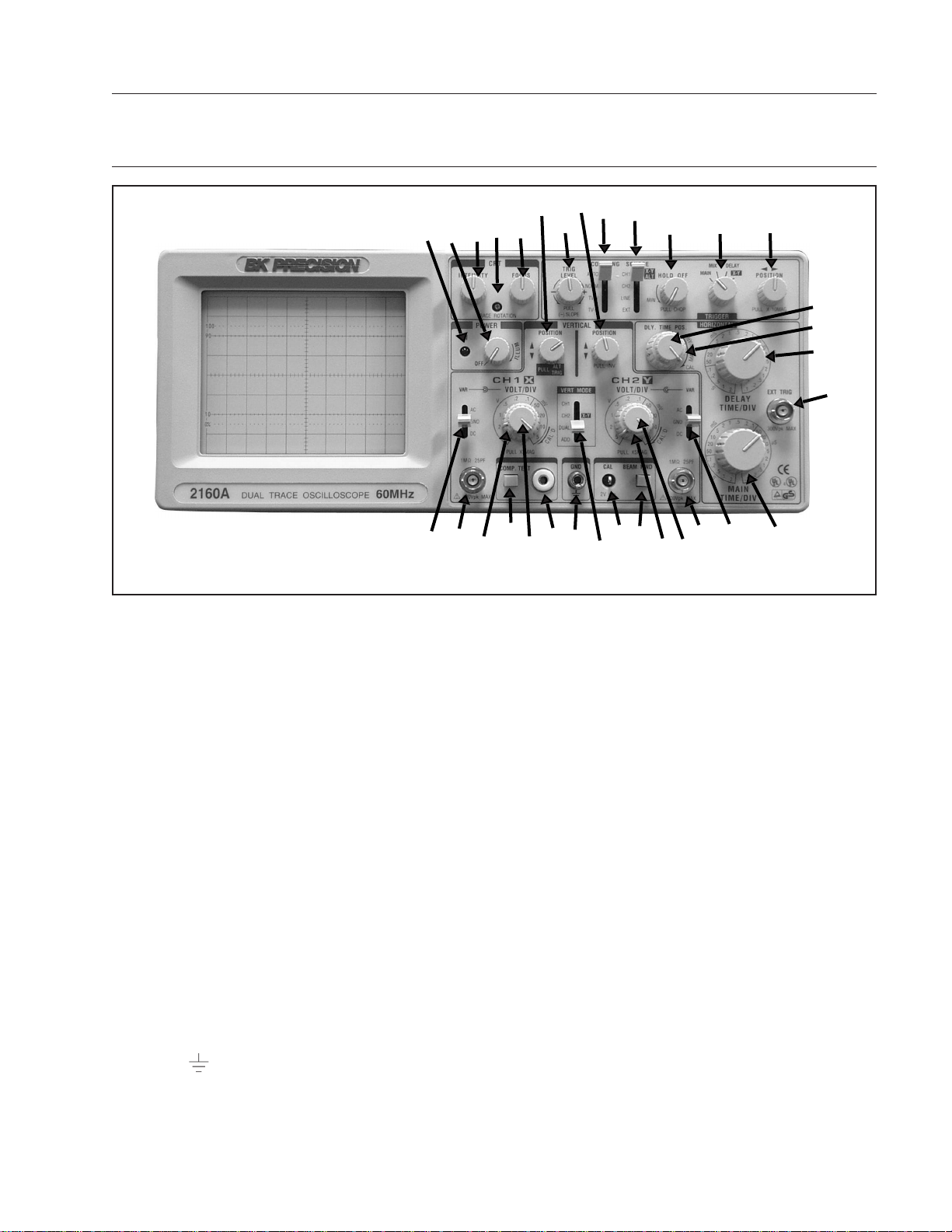
CONTROLS AND INDICATORS

26 25

Fig. 1. Model 2160A Controls and Indicators.

GENERAL FUNCTION CONTROLS

1. ON Indicator. Lights when oscilloscope is “on”.

2. 2160A Only. POWER/Scale ILLUMination Control. Clockwise rotation from OFF position turns os-

cilloscope “on”. Further clockwise rotation increases amount of graticule illumination.

3. 1541D Only. POWER Pushbutton. Turns oscilloscope “on” and “off”.

4. INTENSITY Control. Adjusts brightness of trace.

5. TRACE ROTATION Control. Adjusts to maintain

trace at a horizontal position.

6. FOCUS Control. Adjusts trace focus.

7. 2160A Only. COMPonent TEST Pushbutton. With pushbutton set to “in” position, Component Test mode is enabled. Normal scope operation is enabled with pushbutton in “out” position.

8. 2160A Only. COMPonent TEST Jack. “Banana”type HI-side input jack for connection to component in Component Test operating mode.

9. GND Terminal. Oscilloscope chassis ground jack, and earth ground via three-wire ac power cord. On Model 2160A, also serves as LO-side Component Test jack.

10. CAL Terminal. Terminal provides 2 V p-p, 1 kHz

(nominal) square wave signal. This signal is useful for checking probe compensation adjustment, as well as providing a rough check of vertical calibration.

11. 2160AOnly.BEAM FIND Pushbutton. Momentary-

contact pushbutton speeds setup of trace positioning by bringing the beam into graticule area; operates independently of other display controls.

VERTICAL CONTROLS

12. VERTical MODE Switch. Selects vertical display

mode. Four-position lever switch with the following positions:

CH1:

Displays the channel 1 signal by itself.

CH2/X-Y:

CH2: displays the channel 2 signal by itself. X-Y: used in conjunction with the X-Y control and

Trigger SOURCE switch to enable X-Y display

mode.

DUAL:

Displays the channel 1 and channel 2 signals simultaneously. Dual-trace mode may be either alternate or chop ped sweep; see the description under HOLDOFF/PULL CHOP control.

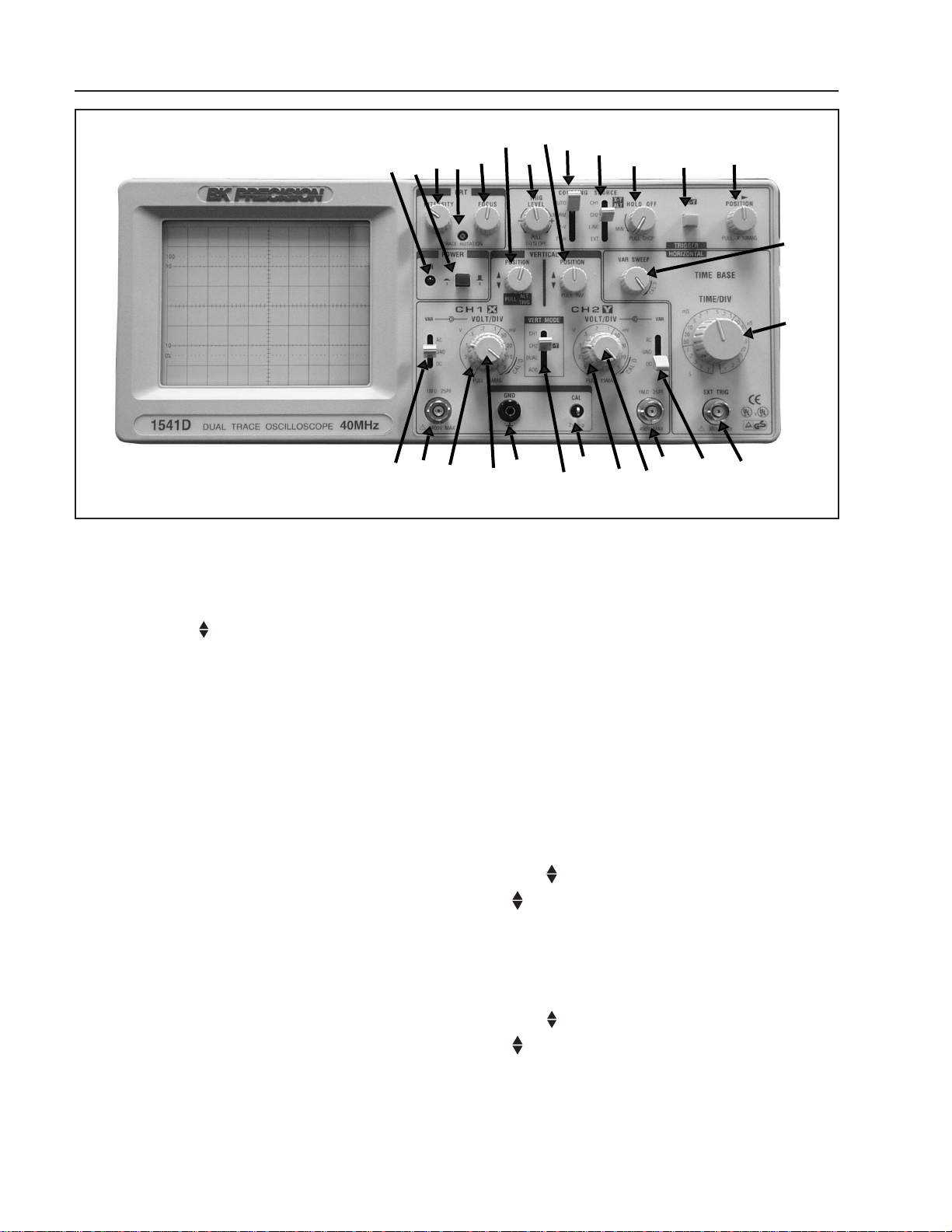
CONTROLS AND INDICATORS

Fig. 2. Model 1541D Controls and Indicators.

ADD:

The inputs from channel 1 and channel 2 are summed and displayed as a single signal. If the Channel 2 POSition/PULL INVert control is pulled out, the input from channel 2 is subtracted from channel 1 and the difference is displayed as a single signal.

13. CH1 AC-GND-DC Switch. Three-position lever

switch with the following positions:

AC:

Channel 1 input signal is capacitively coupled; dc component is blocked.

GND:

Opens signal path and grounds input to vertical amplifier. This provides a zero-volt base line, the position of which can be used as a reference when performing dc measurements.

DC:

Direct coupling of channel 1 input signal; both ac and dc components of signal produce vertical deflection.

14. CH1 (X) Input Jack. Vertical input for channel 1.

X-axis input for X-Y operation.

15. CH1 (X) VOLTS/DIV Control. Vertical attenuator

for channel 1. Provides step adjustment of vertical sensitivity. When channel 1 VARiable control is set to CAL, vertical sensitivity is calibrated in 10 steps from 5 mV/div to 5 V/div in a 1-2-5 sequence. When

the X-Y mode of operation is selected, this control provides step adjustment of X-axis sensitivity.

16. CH1 VARiable/PULL X5 MAG Control: VARiable:

Rotation provides vernier adjustment of channel 1 vertical sensitivity. In the fully-clockwise (CAL) position, the vertical attenuator is calibrated. Counterclockwise rotation decreases gain sensitivity. In X-Y operation, this control becomes the vernier X-axis sensitivity control.

PULL X5 MAG:

When pulled out, increases vertical sensitivity by a factor of five. Effectively provides two extra sensitivity settings: 2 mV/div and 1 mV/div. In X-Y mode, increases X-sensitivity by a factor of five.

17. CH1 POSition/PULL ALT TRIGger Control:

POSition:

Adjusts vertical position of channel 1 trace.

PULL ALT:

Used in conjunction with the Trigger SOURCE switch to activate alternate triggering. See the description under the Trigger SOURCE switch.

18. CH2 POSition/PULL INVert Control:

POSition:

Adjusts vertical position of channel 2 trace. In X-Y operation, rotation adjusts vertical position of X-Y display.

CONTROLS AND INDICATORS

PULL INVert:

When pushed in, the polarity of the channel 2 signal is normal. When pulled out, the polarity of the channel 2 signal is reversed, thus inverting the waveform.

19. CH2 VOLTS/DIV Control. Vertical attenuator for

channel 2. Provides step adjustment of vertical sensitivity. When channel 2 VARiable control is set to CAL, vertical sensitivity is calibrated in 10 steps from 5 mV/div to 5 V/div in a 1-2-5 sequence. When the X-Y mode of operation is selected, this control provides step adjustment of Y-axis sensitivity.

20. CH2 VARiable/PULL X5 MAG Control: VARiable:

Rotation provides vernier adjustment of channel 2 vertical sensitivity. In the fully-clockwise (CAL) position, the vertical attenuator is calibrated. Counterclockwise rotation decreases gain sensitivity. In X-Y operation, this control becomes the vernier Y-axis sensitivity control.

PULL X5 MAG:

When pulled out, increases vertical sensitivity by a factor of five. Effectively provides two extra sensitivity settings: 2 mV/div and 1 mV/div. In X-Y mode, increases Y-sensitivity by a factor of five.

21. CH2 (Y) Input Jack. Vertical input for channel 2. Y-axis input for X-Y operation.

22. CH2 AC-GND-DC Switch. Three-position lever switch with the following positions:

AC:

Channel 2 input signal is capacitively coupled; dc component is blocked.

GND:

Opens signal path and grounds input to vertical amplifier. This provides a zero-volt base line, the position of which can be used as a reference when performing dc measurements.

DC:

Direct coupling of channel 2 input signal; both ac and dc components of signal produce vertical deflection.

HORIZONTAL CONTROLS

23. Main Time Base TIME/DIV Control. Provides step selection of sweep rate for the main time base. When theVARiable Sweep control isset to CAL, sweep rate iscalibrated. This controlhas23 steps, from0.1 µS/div to 2 S/div, in a 1-2-5 sequence.

24. 2160A Only. DELAY Time Base TIME/DIV Control. Provides step selection of sweep rate for delayed

sweep time base. This control has 23 steps, from 0.1 µS/div to 2 S/div, in a 1-2-5 sequence.

25. 2160A Only. DELAY TIMEPOSition Control. Sets

starting point of delayed sweep. Clockwise rotation causes delayed sweep to begin earlier.

26. VARiable Sweep Control. Rotation of control is ver-

nier adjustment for sweep rate. In fully clockwise (CAL) position, sweep rate is calibrated. On the Model 2160A, this control is the vernier adjustment for both the main and delayed time bases.

27. POSition/PULL X10 MAG Control. POSition:

Horizontal (X) position control.

PULL X10 MAG:

Selects ten times sweep magnification when pulled out, normal when pushed in. Increases maximum sweep rate to 10 nS/div.

28. 2160A Only. Sweep Mode Switch. Selects sweep

(horizontal) mode. Four-position rotary switch with the following positions:

MAIN:

Only the main sweep operates, with the delayed sweep inactive.

MIX:

The main and delayed sweep share a single trace; main sweep occupies the left portion of the display; delayed sweep occupies the right portion of the display. The DELAY TIME POSition control de- termines the percentage of display that is main sweep and the percentage of display that is delayed sweep (main sweep is usually brighter than the delayed sweep). Delayed sweep speed cannot be slower than main sweep speed.

DELAY:

Only delayed sweep operates, while main sweep stays inactive. DELAY TIME POSition control determines the starting point of the delayed sweep.

X-Y:

Used with the VERTical MODE switch and Trigger SOURCE switch to select X- Y operating

mode. The channel 1 input becomes the X-axis and the channel 2 input becomes the Y-axis. Trigger source and coupling are disabled in this mode.

29. 1541D Only. X-Y Switch. Used with the VERTical

MODE switch and Trigger SOURCE switch to se-

lect X-Y operating mode. The channel 1 input becomes the X-axis and the channel 2 input becomes the Y-axis. Trigger source and coupling are disabled in this mode.

CONTROLS AND INDICATORS

TRIGGERING CONTROLS

30. HOLDOFF/PULL CHOP Control. HOLDOFF:

Rotation adjusts holdoff time (trigger inhibit period beyond sweep duration). When control is rotated fully counterclockwise, the holdoff period is MIN- inum (normal). The holdoff period increases progressively with clockwise rotation.

PULL CHOP:

When this switch is pulled out in the dual-trace mode, the channel 1 and channel 2 sweeps are chopped and displayed simultaneously (normally used at slower sweep speeds). When it is pushed in, the two sweeps are alternately displayed, one after the other (normally used at higher sweep speeds).

31. Trigger SOURCE Switch. Selects source of sweep

trigger. Four-position lever switch with the following positions:

CH1/X-Y/ALT

CH1:

Causes the channel 1 input signal to become the sweep trigger, regardless of the VERTical

MODE switch setting.

X-Y:

Used with two other switches to enable the X-Y mode — see the Operating Instructions under “XY Operation”.

ALT:

Used with the channel 1 POSition/PULL ALTernate TRIGger control to enable alternate

triggering. Alternate triggering, used in dualtrace mode, permits each waveform viewed to become its own trigger source.

CH2:

The channel 2 signal becomes the sweep trigger, regardless of the VERTicalMODE switch setting.

LINE:

Signal derived from input line voltage (50/60 Hz) becomes trigger.

EXT:

Signal from EXTernal TRIGger jack becomes sweep trigger.

32. Trigger COUPLING Switch. Selects trigger cou-

pling. Four-position lever switch with the following positions:

AUTO:

Selectsautomatic triggeringmode.In this mode,the oscilloscope generates sweep (free runs) in absence of an adequate trigger; it automatically reverts to triggeredsweepoperation when anadequate trigger signal is present. On the Model 2160A, automatic triggering is applicable to both the main sweep and delayed sweep.

NORM:

Selects normal triggered sweep operation. A sweep is generated only when an adequate trigger signal is present.

TV-V:

Used for triggering from television vertical sync pulses. Also serves as lo-pass/dc (high frequency reject) trigger coupling.

TV-H:

Used for triggering from television horizontal sync pulses.Also servesashi-pass (low frequencyreject) trigger coupling.

33. TRIGger LEVEL/PULL (-) SLOPE Control. TRIGger LEVEL:

Trigger level adjustment; determines the point on the triggering waveform where the sweep is triggered. Rotation in the (-) direction (counterclockwise) s elects more negative triggering point; rotation in the (+) direction (clockwise) selects more positive triggering point.

PULL (—) SLOPE:

Two-position push-pull switch. The “in” position selectsa positive-going slope and the “out” position selectsa negative-goingslopeastriggering point for main sweep.

34. EXTernal TRIGger Jack. External trigger input for single- and dual-trace operation.

REAR PANEL CONTROLS (not shown)

35. Fuse Holder/Line Voltage Selector. Contains fuse and selects line voltage.

36. Power Cord Receptacle.

37. 2160A Only. CH 2 (Y) SIGNAL OUTPUT Jack.

Output terminal where sample of channel 2 signal is available.Amplitude of output is nominally 50mVper division of vertical deflection seen on CRT when terminated into 50 Ω. Output impedance is 50 Ω.

38. 2160A Only. Z-Axis Input Jack. Input jack for intensity modulation of CRT electron beam. TTL compatible (5 V p-p sensitivity). Positive levels increase intensity.

39. Handle/Tilt Stand.

40. Feet/Cord Wrap.

OPERATING INSTRUCTIONS

NOTE

All operating instructions in this chapter apply equally to both Models 2160A and 1541D,exceptfor the sectionson“Delayed Sweep Operation” and “Component Test”, which apply only to the Model 2160A. Other differences are noted when necessary.

SAFETY PRECAUTIONS

WARNING

The following precautions must be observed to help prevent electric shock.

1. When the oscilloscope is used to make measurements in equipment that contains high voltage, there is always acertainamountofdangerfromelectricalshock. The person using the oscilloscope in such conditions should be a qualified electronics technician or otherwise trained and qualified to work in such circumstances. Observe the TEST INSTRUMENT SAFETY recommendations listed on the inside front cover of this manual.

2. Donotoperate this oscilloscope with the caseremoved unless you are a qualified service technician. High voltage up to 12,000 volts is present when the unit is operating with the case removed.

3. The ground wire of the 3-wire ac power plug places the chassis and housing of the oscilloscope at earth ground. Use only a 3-wire outlet, and do not attempt to defeat the ground wire connection or float the oscilloscope; to do so may pose a great safety hazard.

4. Specialprecautions are required to measureorobserve line voltage waveforms with any oscilloscope. Use the following procedure:

a. Do not connect the ground clip of the probe to

either side of the line. The clip is already at earth ground and touching it to the hot side of the line may “weld” or “disintegrate” the probe tip and cause possible injury, plus possible damage to the scope or probe.

b. Insert the probe tip into one side of the line voltage

receptacle, then the other. One side of the receptacleshould be “hot” and producethe waveform.The other side of the receptacle is the ac return and no waveform should result.

EQUIPMENT PROTECTION PRECAUTIONS

Thefollowing precautionswill help avoid damage to the oscilloscope.

1. Never allow a small spot of high brilliance to remain stationary on the screen for more than a few seconds. The screen may become permanently burned. A spot will occur when the scope is set up for X−Y operation and no signal is applied. Either reduce the intensity so the spot is barely visible, apply signal, orswitch back to normal sweep operation. It is also advisable to use low intensity with AUTO triggering and no signal applied for long periods. A high intensity trace at the same position could cause a line to become permanently burned onto the screen.

2. Do not obstruct the ventilating holes in the case, as this will increase the scope’s internal temperature.

3. Excessive voltage applied to the input jacks may damage the oscilloscope. The maximum ratings of the inputs are as follows:

CH 1 and CH 2:

400 V dc + ac peak.

EXT TRIG:

300 V dc + ac peak.

Z-AXIS INPUT (Model 2160A):

30 V ( dc and ac peak).

4. Always connect a cable from the ground terminal of the oscilloscope to the chassis of the equipment under test. Without this precaution, the entire current for the equipment under test may be drawn through the probe clip leads under certain circumstances. Such conditionscould also pose a safety hazard,whichthe ground cable will prevent.

5. The probe ground clips are at oscilloscope and earth ground and should be connected only to the earth ground or isolated common of the equipment under test. To measure with respect to any point other than the common, use CH 2 – CH 1 subtract operation (ADD mode and INV 1), with the channel 2 probe to the point of measurement and the channel 1 probe to the point of reference. Use this method even if the reference point is a dc voltage with no signal.

OPERATING INSTRUCTIONS

OPERATING TIPS

The following recommendations will help obtain the best

performance from the oscilloscope.

1. Always use the probe ground clips for best results, attached to a circuit ground point near the point of measurement.Do not rely solely on an externalground wire in lieu of the probe ground clips as undesired signals may be introduced.

2. Avoid the following operating conditions: a. Direct sunlight. b. High temperature and humidity. c. Mechanical vibration. d. Electricalnoise and strong magnetic fields, such as

near large motors, power supplies, transformers, etc.

3. Occasionally check trace rotation, probe compensation,and calibration accuracyofthe oscilloscope using the procedures found in the MAINTENANCE section of this manual.

4. Terminate the output of a signal generator into its characteristic impedance to minimize ringing, especially if the signal has fast edges such as square waves or pulses. For example, the typical 50 Ω output of a square wave generator should be terminated into an external 50 Ω terminating load and connected to the oscilloscope with 50 Ω coaxial cable.

5. Probe compensation adjustment matches the probe to the input of the scope. For best results, compensation should be adjusted initially, then the same probe alwaysusedwith the same channel. Probecompensation should be readjusted when a probe from a different oscilloscope is used.

INITIAL STARTING PROCEDURE

Until you familiarize yourself with the use of all controls, the settings given here can be used as a reference point to obtain a trace on the CRT in preparation for waveform observation.

1. Set these controls as follows: On both models:

VERTical MODE to CH1. CH1AC/GND/DC to GND. Trigger COUPLING to AUTO. Trigger SOURCE to CH1.

All POSition controls and INTENSITY control centered (pointers facing up). Main Time Base control to 1 mS/div.

On the Model 2160A: Sweep Mode switch to MAIN.

2. Press the red POWER pushbutton (Model 1541D), or rotate the POWER control clockwise away from “OFF” (Model 2160A).

3. A trace should appear on the CRT. Adjust the trace brightness with the INTENSITY control, and the trace sharpness with the FOCUS control.

NOTE

On the Model 2160A, you can use the BEAM FINDER pushbutton to locate a trace that has been moved off the screen by the POSition controls. When the button is pushed, a compressed version of the trace is brought into view which indicates the location of the trace.

SINGLE TRACEDISPLAY

Either channel 1 or channel 2 maybe used for single-trace

operation. To observe a waveform on channel 1:

1. Perform the steps of the “Initial Starting Procedure”.

2. Connect the probe to the CH 1 (X) input jack.

3. Connect the probe ground clip to the chassis or common of the equipment under test. Connect the probe tip to the point of measurement.

4. Move the CH1 AC/GND/DC switch out of the GND position to either DC or AC.

5. If no waveforms appear, increase the sensitivity by turning the CH 1 VOLTS/DIV control clockwise to a position that gives 2 to 6 divisions vertical deflection.

6. Position the waveform vertically as desired using the CH1 POSition control.

7. Thedisplay on the CRT maybeunsynchronized.Refer to the “Triggering” paragraphs in this section for procedures on setting triggering and sweep time controls to obtain a stable display showing the desired number of waveforms.

DUAL TRACE DISPLAY

In observing simultaneous waveforms on channel 1 and 2, the waveforms are usually related in frequency, or one of the waveforms is synchronized to the other, although the basic frequencies are different. To observe two such related waveforms simultaneously, perform the following:

1. Connect probes to both the CH 1 (X) and CH 2 (Y)

input jacks.

2. Connect the ground clips of the probes to the chassis or common of the equipment under test. Connect the tips of the probes to the two points in the circuit where waveforms are to be measured.

OPERATING INSTRUCTIONS

3. To view both waveforms simultaneously, set the

VERTical MODE switch to DUAL and select either ALT (alternate) or CHOP with the PULL CHOP

switch.

4. In the ALT sweep mode (PULL CHOP switch

pushed in), one sweep displays the channel 1 signal and the next sweep displays the channel 2 signal in an alternating sequence. Alternate sweep is normally used for viewing high-frequency or high-speed waveforms at sweep times of 1 ms/div and faster, but may be selected at any sweep time.

5. In the CHOP sweep mode (PULL CHOP switch

pulled out), the sweep is chopped (switched) between channel 1 and channel 2. Using CHOP, one channel does not have to “wait” for a complete swept display of the other channel. Therefore, portions of both channel’swaveformsaredisplayedwith the phase relationship between the two waveforms unaltered. Chop sweep is normally used for low-frequency or lowspeed waveforms at sweep times of 1 ms/div and slower; or where the phase relationship between channel 1 and channel 2 requires measurement.

If chop sweep is used at sweep times of 0.2 ms/div and faster, the chop rate becomes a significant portion of the sweep and may become visible in the displayed waveform. However, you may select chop sweep at any sweep time for special applications.

6. Adjust the channel 1 and 2

▲

POSition controls to

▼

place the channel 1 trace above the channel 2 trace.

7. Set the CH 1 and CH 2 VOLTS/DIV controls to a

position that gives 2 to 3 divisions of vertical deflection for each trace. If the display on the screen is unsynchronized, refer to the “Triggering” paragraphs in this section of the manual for procedures for setting triggering and sweep time controls to obtain a stable display showing the desired number of waveforms.

8. WhentheVERTicalMODE switch is set to ADD, the

algebraic sum of CH 1 + CH 2 is displayed as a single trace. When the PULL INV switch is pulled out, the algebraic difference of CH 1 – CH 2 is displayed.

9. Iftwowaveformshavenophaseorfrequencyrelationship, there is seldom reason to observe both waveforms simultaneously. However, these oscilloscopes do permit the simultaneous viewing of two such unrelated waveforms, using alternate triggering. Refer to the paragraphs on “Triggering - Trigger SOURCE Switch”, for details on alternate triggering.

TRIGGERING

The Models 2160A and 1541D Oscilloscopes provide versatility in sync triggering for ability to obtain a stable, jitter-free display in single-trace, or dual-trace operation. The proper settings depend upon the type of waveforms being observed and the type of measurement desired. An explanation of the various controls which affect synchronization is given to help you select the proper setting over a wide range of conditions.

Trigger COUPLING Switch

1. In the AUTO position, automatic sweep operation is

selected. In automatic sweep operation, the sweep generator free-runs to generate a sweep without a trigger signal. However, it automatically switches to triggered sweep operation if an acceptable trigger source signal is present. The AUTO position is handy when first setting up the scope to observe a waveform; itprovides sweepforwaveform observationuntilother controls can be properly set. Once the controls are set, operation is often switched back to the normal triggering mode, since it is more sensitive. Automatic sweep must be used for dc measurements and signals of such low amplitude that they will not trigger the sweep.

2. The NORM position provides normal triggered

sweep operation. The sweep remains at rest until the selected trigger source signal crosses the threshold level set by the TRIG LEVEL control. The trigger causes one sweep to be generated, after which the sweep again remains at rest until triggered. In the normal triggering mode, there will be no trace unless an adequate trigger signal is present. In the ALT

VERTICAL MODE of dual trace operation with the SOURCE switch also set to ALT, there will be no

trace unless both channel 1 and channel 2 signals are adequate for triggering. Typically, signals that produce even one division of vertical deflection are adequate for normal triggered sweep operation.

3. The TV H and TV V positions are primarily for

viewing composite video waveforms. Horizontal sync pulses are selected as trigger when the trigger COU- PLINGswitch is set to the TV H position, and vertical sync pulses are selected as trigger when the trigger

COUPLING switch is set to the TV V position. The TV H and TV V positions may also be used as low

frequency reject and high frequency reject coupling, respectively. Additional procedures for observing video waveforms are given later in this section of the manual.

OPERATING INSTRUCTIONS

Trigger SOURCE Switch

The trigger SOURCE switch (CH 1, CH 2, etc.) selects

the signal to be used as the sync trigger.

1. If the SOURCE switch is set to CH 1 (or CH 2) the

channel 1 (or channel 2) signal becomes the trigger source regardless of the VERTICAL MODE selection.CH 1,orCH 2 are often used as the triggersource for phase or timing comparison measurements.

2. By setting the SOURCE switch to ALT (same as CH1) and PULL ALT TRIG pulled, alternating triggering mode is activated. In this mode, the trigger source alternates between CH 1 and CH 2 with each sweep. This is convenient for checking amplitudes, waveshape, or waveform period measurements, and even permits simultaneous observation of two waveforms which are not related in frequency or period. However,this setting isnot suitable forphase or timing comparison measurements. For such measurements, both traces must be triggered by the same sync signal. Alternate triggering can only be used in dual-trace mode (VERT MODE set to DUAL), and with alternate sweep only (PULL CHOP not engaged).

3. In the LINE position, triggering is derived from the input line voltage (50/60 Hz) and the trigger SOURCE switch is disabled. This is useful for measurements that are related to line frequency.

4. In the EXT position, the signal applied to the EXT TRIG jack becomes the trigger source. This signal must have a timing relationship to the displayed waveforms for a synchronized display.

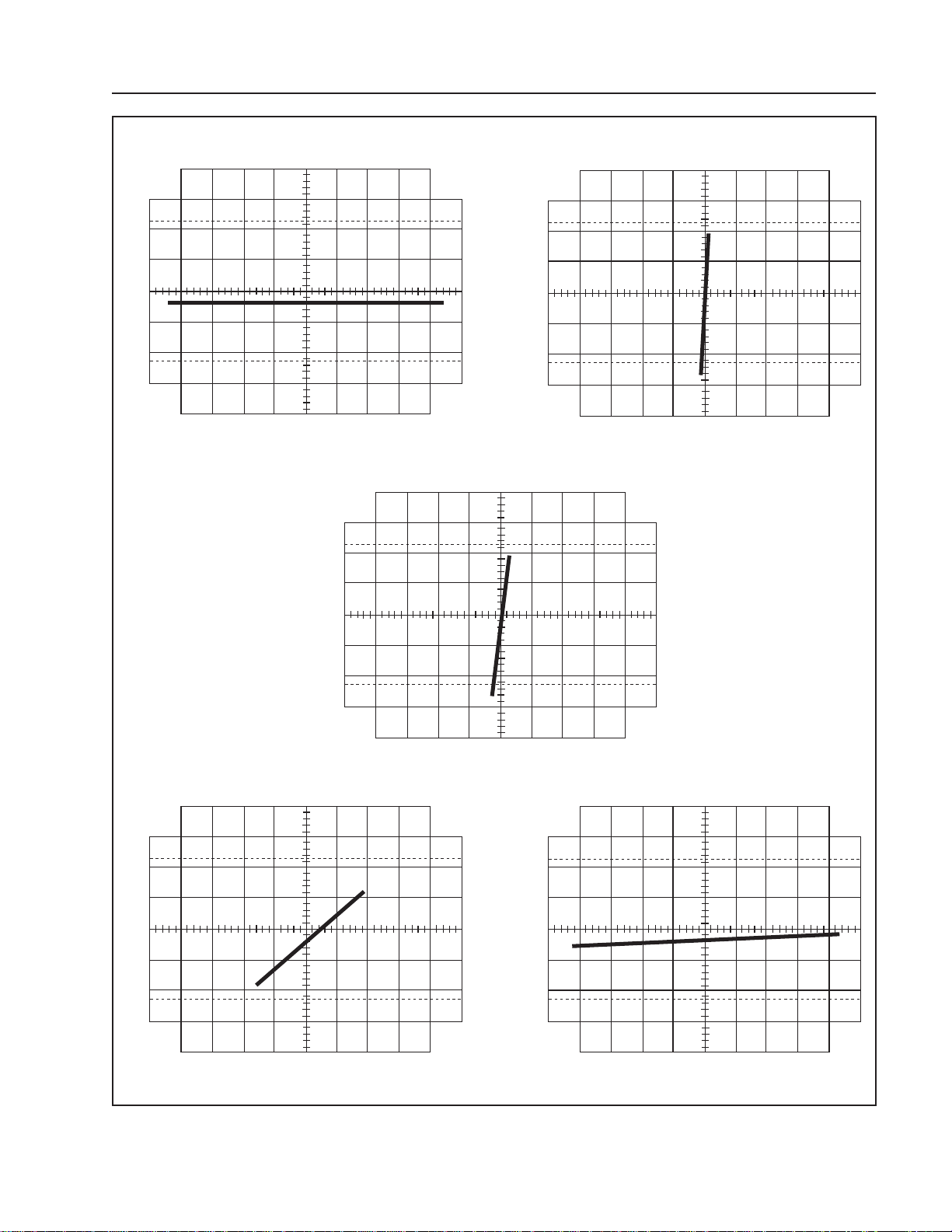
TRIG LEVEL/PULL (–) SLOPE Control

(Refer to Fig. 3)

A sweep trigger is developed when the trigger source

signalcrosses a preset threshold level.Rotation of the TRIG LEVEL control varies the threshold level. In the + direction (clockwise), the triggering threshold shifts to a more positive value, and in the − direction (counterclockwise), the triggering threshold shifts to a more negative value. When

the control is centered, the threshold level is set at the approximate average of the signal used as the triggering source. Proper adjustment of this control usually synchronizes the display.

The TRIG LEVEL control adjusts the start of the sweep

to almost any desired point on a waveform. On sine wave signals, the phase at which sweep begins is variable. Note that if the TRIG LEVEL control is rotated toward its extreme + or − setting, no sweep will be developed in the normal trigger mode because the triggering threshold exceeds the peak amplitude of the sync signal.

When the PULL (–) SLOPE control is set to the + (“in”)

position, the sweep is developed from the trigger source waveform as it crosses a threshold level in a positive-going direction. When the PULL (–) SLOPE control is set to the −(“out”) position, a sweep trigger is developed from the trigger source waveform as it crosses the threshold level in a negative-going direction.

MAIN TIME BASE Control

Set the Main Time Base TIME/DIV control to display

the desired number of cycles of the waveform. If there are too many cycles displayed for good resolution, switch to a faster sweep time. If only a line is displayed, try a slower sweep time. When the sweep time is faster than the waveform being observed,only part of it will be displayed, which may appear as a straight line for a square wave or pulse waveform.

HOLDOFF Control

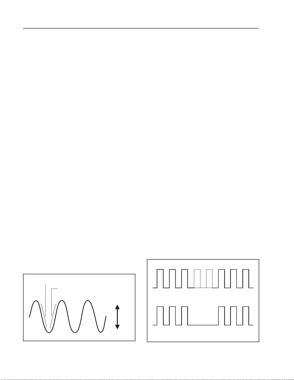
(Refer to Fig. 4)

A “holdoff” period occurs immediately after the completion of each sweep, and is a period during which triggering of the next sweep is inhibited. The normal holdoff period varies with sweep rate, but is adequate to assure complete retrace and stabilization before the next sweep trigger is permitted. The HOLDOFF control allows this period to be extended by a variable amount if desired.

Slope “–” Range

Slope “+” Range

Level

–

Fig. 3. Function of Slope and Level Controls.

A. Holdoff not used

B. Holdoff used

Fig. 4. Use of HOLDOFF Control.

OPERATING INSTRUCTIONS

This control is usually set to the MIN position (fully

counterclockwise) because no additional holdoff period is necessary. The HOLDOFF control is useful when a complex series of pulses appear periodically such as in Fig. 4B. Improper sync may produce a double image as in Fig. 4A. Such a display could be synchronized with the VA R SWEEP control, but this is impractical because time measurements are then uncalibrated. An alternate method of synchronizing the display is with the HOLDOFF control. The sweep speed remains the same, but the triggering of the next sweep is “held off” for the duration selected by the HOLDOFF control. Turn the HOLDOFF control clockwise from the MIN position until the sweep starts at the same point of the waveform each time.

MAGNIFIED SWEEP OPERATION

Since merely shortening the sweep time to magnify a portion of an observed waveform can result in the desired portion disappearing off the screen, magnified display should be performed using magnified sweep.

Using the POSition control, move the desired portion of waveformto the center of the CRT. Pull out the PULL X10 knob to magnify the display ten times. For this type of display the sweep time is the Main Time Base TIME/DIV control setting divided by 10. Rotation of the POSition control can then be used to select the desired portion of the waveforms.

X−Y OPERATION

X−Y operation permits the oscilloscope to perform many measurements not possible with conventional sweep operation. The CRT display becomes an electronic graph of two instantaneous voltages. The display may be a direct comparison of the two voltages such as stereoscope display of stereo signal outputs. However, theX−Y mode can be used to graph almost any dynamic characteristic if a transducer is used to change the characteristic (frequency, temperature, velocity, etc.) into a voltage. One common application is frequencyresponse measurements,where the Yaxis correspondsto signal amplitude and the X axis corresponds to frequency .

1. On the Model 2160A, set the SWEEP MODE switch

totheX−Yposition. On the Model 1541D, depress the X−Y switch. On both models, set the Trigger Source and VERTical MODE switches to X−Y.

2. In this mode, channel 1 becomes the X axis input and channel 2 becomes the Y axis input. The X and Y positionsare now adjusted usingthe POSitionand the channel 2 POSition controls respectively.

3. Adjust the amount of vertical (Y axis) deflection with the CH 2 VOLTS/DIV and VARIABLE controls.

4. Adjust the amount of horizontal (X axis) deflection with the CH 1 VOLTS/DIV and VARIABLE controls.

VIDEO SIGNAL OBSERVATION

Setting the COUPLING switch to the TV-H or TV-V

position permits selection of horizontal or vertical sync pulses for sweep triggering when viewing composite video waveforms.

When the TV-H mode is selected, horizontal sync pulses

are selected as triggers to permit viewing of horizontal lines of video. A sweep time of about 10 µs/div is appropriate for displaying lines of video. The VAR SWEEP control can be set to display the exact number of waveforms desired.

When the TV-Vmode is selected, verticalsync pulses are

selected as triggers to permit viewing of vertical fields and frames of video. A sweep time of 2 ms/divis appropriate for viewing fields of video and 5 ms/div for complete frames (two interlaced fields) of video.

At most points of measurement, a composite video signal

is of the (−)polarity, that is, the sync pulses are negative and the video is positive. In this case, use (− ) SLOPE. If the waveform is taken at a circuit point where the video waveform is inverted, the sync pulses are positive and the video is negative. In this case, use (+) SLOPE.

APPLICATIONS GUIDEBOOK

B+K Precision offers a “Guidebook to Oscilloscopes”

which describes numerous applications for this instrument and important considerations about probes. It includes a glossary of oscilloscope terminology and an understanding of how oscilloscopes operate. It may be downloaded free of charge from our Website, www.bkprecision.com.

DELAYED SWEEP OPERATION (Model 2160A)

(Refer to Fig. 5)

Delayed sweep operation is achieved by use of both the

main sweep and the delayed sweep and allows any portion of a waveform to be magnified for observation. Unlike X10 magnification, delayed sweep allows selectable steps of magnification.

1. SettheSweepMode switch to the MAIN position and

adjust the oscilloscope for a normal display.

2. Set the Sweep Mode switch to the MIX position. The

display will show the main sweep on the left portion (representing the MAIN Time Base control setting) and the delayed sweep on the right portion (representing the DELAY Time Base control setting). The MAIN Time Base portion of the trace usually will be brighter than the delayed time base portion. Fig. 5 shows a typical display for the MIX display mode.

3. Shift the percentage of the display that is occupied by

the main sweep by adjusting the DELAY TIME POSition control. Counterclockwise rotation causes more of the display to be occupied by the main sweep

OPERATING INSTRUCTIONS

Delayed Sweep

100

Main

Sweep

Fig. 5. MIX SWEEP MODE Display.

and clockwise rotation causes more of the display to be occupied by the delayed sweep.

4. Set the Sweep Mode switch to the DELAY position

to display only the magnified delayed sweep portion of the display.

NOTE

In order to obtain meaningful results with delayed sweep, the DELAY Time Base control must set be set to a faster sweep speed than the MAIN Time Base control. Because of this, the oscilloscope automatically prevents (electrically) the DELAY Time Base from being set to a slower sweep speed than the MAIN Time Base. Forexample, if the MAINTimeBase is set to0.1 ms/div, theslowest possibleDELAY TimeBase sweep speed is also 0.1ms/div, even if the control is set slower.

COMPONENT TEST OPERATION

(Model 2160A)

Do not apply an external voltage to the COMP TEST jacks. Only non-powered circuits should be tested with this unit. Testing powered circuits could damage the instrument and increase the risk of electrical shock.

The component test function produces a component “signature” on the CRT by applying an ac signal across the device and measuring the resulting ac current. The display represents a graph of voltage (X) versus current (Y). The

component test function can be used to view the signatures of resistors, capacitors, inductors, diodes, and other semiconductor devices. Devices may be analyzed in-circuit or out-of-circuit and combinations of two or more devicesmay be displayed simultaneously. Each component produces a different signature and the components can be analyzed as outlined below.

Component Test mode is activated by depressing the

COMPonent TEST switch. The SWEEP MODE switch must not be in the DELAY position.

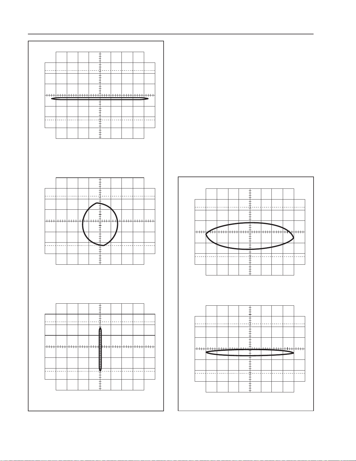
Resistors

A purely resistive impedance produces a signature that is a straight line. A short circuit produces a vertical line and an open circuit causes a horizontal line. Therefore, the higher the resistance, the closer to horizontal the trace will be. Values from 10 Ω to about 5 kΩ are within measurement range. Values below 10 Ω will appear to be a dead short while values above 5 kΩ will appear to be an open circuit. Fig. 6 shows some typical resistance signatures.

To test a resistor,insertone of the resistor’sleads into the white COMP TEST jack, and the other into the GND jack (make sure that the leads touch the metal walls inside the jacks). To test in-circuit, a pair of test leads can be used to connect the COMP TEST and GND jacks to the component(s).

Capacitors

Besureto dischargecapacitors (by shorting the leads together) before connecting to the COMP TEST jack. Some capacitors can retain a voltage high enough to damage the instrument.

A purely capacitive impedance produces a signature that is an ellipse or circle. Value is determined by the size and shape of the ellipse. A very low capacitance causes the ellipse to flatten out horizontally and become closer to a straight horizontal line and a very high capacitance causes the ellipse to flatten out vertically and become closer to a straight vertical line. Values from about 0.33 µF to about 330 µF are within measurable range. Values below 0.33 µF will be hard to distinguish from an open circuit and values above330 µF will be hard to distinguish from ashort circuit. Fig. 7 shows several typical capacitance signatures.

To test a capacitor,insert the capacitor’spositive lead into the white COMP TEST jack, and the negative lead into the GND jack (make sure that the leads touch the metal walls inside the jacks). Totest in-circuit or to test a capacitor with leadsthat aretoo short tofit intotheCOMPTESTand GND jacks, a pair of test leads can be used to connect the COMP TEST and GND jacks to the component(s).

OPERATING INSTRUCTIONS

100

Open Circuit

100

Short Circuit

100

10 Resistor

Ω

100

200 Resistor

Ω

5.1 k ResistorΩ

Fig. 6. Typical Resistive Signatures.

OPERATING INSTRUCTIONS

100

0.33 F Capacitorµ

100

Inductors

Like capacitance, a purely inductive impedance produces asignaturethat is an ellipse or circle and valueis determined by the size and shape of the ellipse. A very high inductance causes the ellipse to flatten out horizontally and a very low inductance causes the ellipse to flatten out vertically.Values from about 0.05 H to about 5 H are within measurement range. Values below 0.05 H will be hard to distinguish from a short circuit and values above 5 H will be hard to distinguish from an open. Fig. 8 shows several typical inductance signatures.

To test an inductor, insert one of the inductor’s leads into the white COMP TEST jack, and the other into the GND jack (make sure that the leads touch the metal walls inside the jacks). To test in-circuit or to test an inductor with leads that are too short to be inserted into the COMP TEST and

GND jacks, a pair of test leads can be used to connect the COMP TEST and GND jacks to the component(s).

100

4.7 F Capacitorµ

1 Henry Inductor

100

300 F Capacitorµ

5 Henry Inductor

Fig. 7. Typical Capacitive Signatures.

Fig. 8. Typical Inductive Signatures.

Semiconductors

Purelysemiconductordevices (such as diodes and transistors) will produce signatures with straight lines and bends. Typical diode junctions produce a single bend with a horizontal and vertical line as shown in Fig. 9. Zener diodes produce a double bend with two vertical and one horizontal line as shown in Fig. 10 (value is determined by the distance of the leftmost vertical component from the center graduation on the CRT). The maximum Zener voltage observable on this feature is about 15 V. It is also possible to test transistors and IC’s by testing one pair of pins at a time.

NOTE

When testing diodes it is important to connect the diode’s cathode to the white

COMP TEST jack and the anode to the GNDjack.Reversing thepolaritywill not

damage the devicebut the horizontal and vertical components of the signature will appear in different quadrants of the display.

To test semiconductors, insert the diode’s or transistor’s leads (only two at a time) into the COMP TEST and GND jacks (make sure that the leads touch the metal walls inside the jacks). To test in-circuit or to test IC’s or devices with leads too short to insert into the COMP TESTand GND jacks, a pair of test leads can be used to connect the COMP TEST and GND jacks to the component(s).

OPERATING INSTRUCTIONS

100

Silicon Diode

Fig. 9. Typical P-N Junction Signature.

100

Combinations of Components

Using the component test feature it is also possible to observe the signatures of combinations of components. Combinations cause signatures that are a combination of the individual signatures for each component. For example, a signature for a resistor and capacitorin parallel will produce a signature with the ellipse of the capacitor but the resistor would cause the ellipse to be at an angle (determined by the valueof the resistor). When testing combinations of components it is important to make sure that all the components being connected are within measurement range.

In-CircuitTesting

The component test feature can be very effectivein locating defective components in-circuit, especially if a “known good” piece of equipment is available for reference. Compare the signatures from the equipment under test with signatures from identical points in the reference unit. When

10 V Zener Diode

Fig. 10. Typical Zener Signature.

signaturesare identical orverysimilar,the tested component is good. When signatures are distinctively different, the tested component is probably defective.

MAINTENANCE

WARNING

The following instructions are for use by qualifiedservice personnel only. Toavoid electricalshock,do not perform any servicing other than contained in the operating instructions unless you are qualified to do so.

High voltage up to 12,000 V is present when covers are removed and the unit is operating. Remember that high voltage may be retained indefinitely on high voltage capacitors. Also remember that ac line voltage is present on line voltage input circuits any time the instrument is plugged into an ac outlet, even if turned off. Unplug the oscilloscope and discharge high voltage capacitors before performing service procedures.

FUSE REPLACEMENT

If the fuse blows, the “ON” indicator will not light and the oscilloscope will not operate. The fuse should not normally open unless a problem has developed in the unit. Try to determine and correct the cause of the blown fuse, then replace only with the correct value fuse. For 110/125 V line voltage operation, use an 800 mA, 250 V fuse. For 220/240 Vline voltage operation, use a 600 mA,250Vfuse. The fuse is located on the rear panel adjacent to the power cord receptacle.

PERIODIC ADJUSTMENTS

Probe compensation and trace rotation adjustments should be checked periodically and adjusted if required. These procedures are given below.

Probe Compensation

1. Connectprobes toCH1 andCH2 input jacks.Perform

procedure for each probe, one probe at a time.

2. Set the probe to X10 (compensation adjustment is not possible in the X1 position).

3. Touch tip of probe to CAL terminal.

4. Adjust oscilloscope controls to display 3 or 4 cycles of CAL square wave at 5 or 6 divisions amplitude.

5. Adjust compensation trimmer on probe for optimum square wave (minimum overshoot, rounding off, and tilt). Refer to Fig. 11.

Correct Compensatio

Over Compensatio

Insufficient Compensatio

Remove the fuseholder assembly as follows:

1. Unplug the power cord from rear of scope.

2. Insert a small screwdriver in fuseholder slot (located between fuseholder and receptacle). Pry fuseholder away from receptacle.

3. When reinstalling fuseholder, be sure that the fuse is installedso that the correct line voltage is selected(see LINE VOLTAGE SELECTION).

LINE VOLTAGE SELECTION

To select the desired line voltage, simply insert the fuse and fuse holder so that the appropriate voltage is pointed to by the arrow. Be sure to use the proper value fuse (see label on rear panel).

Fig. 11. Probe Compensation Adjustment.

Trace Rotation Adjustment

1. Set oscilloscope controls for a single trace display in

CH 1 mode, and with the channel 1 AC-GND-DC switch set to GND.

2. Use the channel 1 POSition control to position the trace over the center horizontal line on the graticule scale. The trace should be exactly parallel with the horizontal line.

3. Usethe TRACEROTATIONadjustmenton the front panel to eliminate any trace tilt.

MAINTENANCE

CALIBRATION CHECK

A general check of calibration accuracy may be made by

displaying the output of the CAL terminal on the screen. Thisterminalprovidesa square wave of 2 V p-p. This signal should produce a displayed waveform amplitude of four divisions at .5 V/div sensitivity for both channel 1 and 2 (with probes set for direct). With probes set for X10, there should be four divisions amplitude at 50 mV/div sensitivity. The VARIABLE controls must be set to CAL during this check.

NOTE

The CAL signal should be used only as a general check of calibration accuracy,not as a signal source for performing recalibration adjustments; a voltage standard calibrated at several steps and of 0.3% or better accuracy is required for calibration adjustments.

The CAL signal should not be used as a time base standard.

INSTRUMENT REPAIR SERVICE

Because of the specialized skills and test equipment re-

quired for instrument repair and calibration, many customers prefer to rely upon B+K Precision for this service. To use this service, even if the oscilloscope is no longer under warranty, follow the instructions given in the SERVICE INFORMATION portion of this manual. There is a flat rate charge for instruments out of warranty.

APPENDIX

IMPORTANT CONSIDERATIONS FOR RISE TIME

AND FALL TIME MEASUREMENTS

Error in Observed Measurement

The observed rise time (or fall time) as seen on the CRT is actually the cascaded rise time of the pulse being measured and the oscilloscope’sownrisetime. The two rise times are combined in square law addition as follows:

observed

(T ) +(T )

pulse

scope

The effect of the oscilloscope’s rise time is almost negligible when its rise time is at least 3 times as fast as that of the pulse being measured. Thus, slower rise times may be measured directly from the CRT. However, for faster rise time pulses, an error is introduced that increases progressively as the pulse rise time approaches that of the oscilloscope. Accurate measurements can still be obtained by calculation as described below.

Direct Measurements

TheModel2160A oscilloscope has aratedrisetime of 5.8 ns (8.8 ns for Model 1541D). Thus, pulse rise times of about 17 ns or greater can be measured directly (26 ns for Model 1541D). Most fast rise times are measured at the fastest sweep speed and using X10 magnification. For the Models 2160A and 1541D, this sweep rate is 10 ns/div. A rise time of less than about two divisions at this sweep speed should be calculated for Model 2160A (three divisions for Model 1541D).

Calculated Measurements

Forobserved rise times of lessthan17 ns(26nsforModel 1541D),the pulserisetimeshouldbecaluclated to eliminate the error introduced by the cascaded oscilloscope rise time. Calculate pulse rise time as follows:

pulse

(T ) +(T )

observed

scope

Limits of Measurement

Measurements of pulse rise times that are faster than the scope’srated rise time are not recommended because a very small reading error introduces significant error into the calculation. This limit is reached when the “observed” rise time is about 1.3 times greater than the scope’s rated rise time, about 7.5 ns minimum for the Model 2160A and 12 ns for Model 1541D.

Probe Considerations

Forfast rise timemeasurementswhich approach the limits of measurement, direct connection via 50 Ω coaxial cable and 50 Ω termination is recommended where possible. When a probe is used, its rise time is also cascaded in square law addition. Thus the probe rating should be considerably faster than the oscilloscope if it is to be disregarded in the measurement.

Service Information

Warranty Service: Please return the product in the original packaging with proof of purchase to the address below. Clearly state in writing the performance problem and return any leads, probes, connectors and accessories that you are using with the device.

Non-Warranty Service: Return the product in the original packaging to the address below. Clearly state in writing the performance problem and return any leads, probes, connectors and accessories that you are using with the device. Customers not on open account must include payment in the form of a money order or credit card. For the most current repair charges please visit www.bkprecision.com and click on “service/repair”.

Return all merchandise to B&K Precision Corp. with pre-paid shipping. The flat-rate repair charge for Non-Warranty Service does not include return shipping. Return shipping to locations in North American is included for Warranty Service. For overnight shipments and non-North American shipping fees please contact B&K Precision Corp.

B&K Precision Corp.

22820 Savi Ranch Parkway

Yorba Linda, CA 92887

www.bkprecision.com

714-921-9095

Include with the returned instrument your complete return shipping address, contact name, phone number and description of problem.

Limited Three-Year Warranty

B&K Precision Corp. warrants to the original purchaser that its products and the component parts thereof, will be free from defects in workmanship and materials for a period of three years from date of purchase.

B&K Precision Corp. will, without charge, repair or replace, at its option, defective product or component parts. Returned product must be accompanied by proof of the purchase date in the form of a sales receipt.

To obtain warranty coverage in the U.S.A., this product must be registered by completing a warranty registration form on www.bkprecision.com within fifteen (15) days of purchase.

Exclusions: This warranty does not apply in the event of misuse or abuse of the product or as a result of unauthorized alterations or repairs. The warranty is void if the serial number is altered, defaced or removed.

B&K Precision Corp. shall not be liable for any consequential damages, including without limitation damages resulting from loss of use. Some states do not allow limitations of incidental or consequential damages. So the above limitation or exclusion may not apply to you.

This warranty gives you specific rights and you may have other rights, which vary from state-to-state.

B&K Precision Corp. 22820 Savi Ranch Parkway Yorba Linda, CA 92887 www.bkprecision.com 714-921-9095

B+K Precision

OSCILOSCOPIOS

Models 2120B – 30 MHz 2125A – 30 MHz

1541D – 40 MHz

2160A – 60 MHz

2190B – 100 MHz

=============================================================================

DESCRIPCION

Los Osciloscopios B&K Precision de la serie PS comprenden 5 modelos con ancho de banda de 30; 40; 60 y 100 MHz ( para una atenuación de 3 dB ), con diferentes prestaciones en cada modelo. Aparte de las diferencias de ancho de banda, los modelos presentan diferencias funcionales entre sí, indicándose algunas de ellas en la tabla siguiente. Para facilitar el uso de este manual, la tabla incorpora una guía rápida para ubicar la página correspondiente a los textos relevantes para las funciones adicionales de cada modelo.

Modelo

Pag.

2120B 30 MHz Simple 150 mm - Interna 2125A 30 MHz Demorada 150 mm - Interna

Ancho

Banda

Base de

Tiempo

Tubo / Retícula Multímetro

Digital

No No No No No Si No Si

Salida

Canal 2

Readout

en TRC

Probador

Comp.

Iluminada

1541D 40 MHz Simple 150 mm - Interna

2160A 60 MHz Demorada 150 mm - Interna

No No No No No Si No Si

Iluminada

2190B 100 MHz Demorada 150 mm - Interna

No Si No Si

=============================================================================

CARACTERISTICAS DESTACADAS DE LA SERIE

Facilidad de operación: los controles y el panel frontal han sido diseñados teniendo en cuenta el

agrupar convenientemente los controles relacionados entre sí por su función, facilitando su ubicación y uso. El panel posee varias áreas codificadas en diferentes colores para facilitar al usuario la identificación, ubicación y uso de los distintos comandos disponibles. Alta impedancia de entrada: la impedancia de entrada de ambos canales es, en todos los modelos, de 1 M Ω +/- 2 % en paralelo con 25 pF +/- 10 pF.

Alta sensibilidad : 1 mV / Div. Máximo en todos los modelos. Hold-off variable: disponible en todos los modelos, permite inhibir la generación de pulsos de

disparo de la base de tiempo por un tiempo variable a voluntad, en condición de señales complejas, permitiendo lograr un display estable y repetible. Operación X – Y : seleccionando este modo, el canal 1 se convierte en canal X y el canal 2 en Y permitiendo graficar señales relacionadas entre sí. Disparo de TV: la serie posee separadores de sincronismo para disparo sobre las señales de TV –V y TV -H.

Barrido mezclado (modelos 2125A, 2160A, 2190B): esta función permite ver ambos barridos a continuación uno de otro.

Salida de canal 2: (modelos 2125A, 2160A, 2190B): conector BNC en el panel posterior para extracción de señal de canal 2 para lecturas de frecuencia, etc.

Modulación de intensidad (modelos 2125A, 2160A, 2190B): permite modular la intensidad del haz mediante una señal externa de nivel TTL.

Comprobador de componentes (modelos 2125A, 2160A, 2190B): permite determinar su condición en base a la generación y presentación de una curva característica de corriente en función de la tensión aplicada. Localizador de haz: (modelos 2125A, 2160A, 2190B): permite ubicar el haz dentro de la pantalla irrespectivamente de la posición de los controles de posición, reduciendo el rango de actuación de estos. Retícula iluminada: (modelos 2125A, 2160A, 2190B): facilita la observación de formas de onda en lugares con iluminación pobre. La intensidad es ajustable a conveniencia del usuario.

Barrido de alta velocidad : hasta 10 nSeg / Div ( con magnificador x 10 ) Mod. 2190B: hasta 2 ns / div. con magnificador x 10.

Exactitud : ±3% para sensibilidad , y barrido. Display : rectangular de 150 mm de diagonal, lo que asegura excelente observación de formas de

onda ; aceleración: 2 KV ( 2120B y 2125A ); 8,5 KV ( 1541D ); 12 KV ( 2160A ) y 16 KV ( 2190B ).

=========================================================================

ESPECIFICACIONES

MODELOS

2120B; 2125A; 1541D; 2160A; 2190B

PANTALLA

Tubo rectangular de 150 mm de diagonal, aluminizado. Retícula interna de 8 x 10 div. de 10 mm de lado. Marcas de referencia para 0; 10 %; 90 % y 100 % para verificación de tiempos de establecimiento y atenuación. Ejes centrales con marcas cada 0,2 div. ( 2 mm ). Aceleración simple en mod. 20 y 25 MHz. Modelos de 40; 60 y 100 MHz con posaceleración.

MODELO ACEL. / POSACELERACION

2120B y 2125A 2 KV

1541D 2 KV / 8,5 KV

2160A 2 KV / 12 KV

2190B 2 KV / 16 KV

VERTICAL

Dos canales idénticos; conectores BNC en la entrada. Acoplamiento seleccionable de CA ó CC; posibilidad de conectar a masa la entrada.

Modelo Ancho de banda normal /

Tiempo de establecimiento

Ancho de banda magnificado/

Tiempo de establecimiento

2120B y 2125A 30 MHz ( - 3 dB ) 17,5 ns 5 MHz ( - 3 dB ) 70 ns

1541D 40 MHz ( - 3 dB ) 8,8, ns 10 MHz ( - 3 dB ) 35 ns

2160A 60 MHz ( - 3 dB ) 5,8 ns 15 MHz ( - 3 dB ) 23,2 ns

2190B 100 MHz ( - 3 db ) 3,5 ns 25 MHz ( - 3 dB ) 14 ns

Sensibilidad:

Modelo Sensibilidad normal Sensibilidad magnificado

2120B y 2125A 5 mV a 5 V / div. 1 mV a 1 V / div @ 5 MHz

1541D 5 mV a 5 V / div. 1 mV a 1 V / div @ 10 MHz

2160A 5 mV a 5 V / div. 1 mV a 1 V / div @ 15 MHz

2190B 5 mV a 5 V / div. 1 mV a 1 V / div @ 25 MHz

Atenuador: compensado en frecuencia; secuencia 1-2-5; 10 pasos con ajuste variable contínuo

entre pasos con relación 1:3 (mínimo).

Impedancia: 1 M Ω +/- 2% en paralelo con 25 pF +/-10% todos los modelos. Tensión máxima de entrada: 400 V CC + pico de CA todos los modelos. Sobreimpulso: > 5% Modo Vertical: CH 1; CH2; DUAL ( seleccionable Alternado ó Chopeado ) Modo Suma: CH 1 + CH 2 ó CH 1 – CH 2 ( con canal 2 invertido ) Inversión de polaridad: solo para canal 2

HORIZONTAL Modo X – Y : seleccionable; CH 1 corresponde a X y CH 2 a Y. Exactitud: Eje Y +/- 3 % ; Eje X: +/- 6 % . Ancho de banda del amplificador Horizontal:: CC a 1 MHz – 3 dB Diferencia de fase en modo X - Y: aprox. 3 ° @ 50 KHz todos los modelos excepto 2190B aprox. 3 °

@ 100 KHz.

BARRIDO Modo de barrido:

Modelos 2120B con base de tiempo única, no presenta opción. Modelos 2125A; 2160A y 2190B con doble base de tiempos : Main ( principal ); Mix , Delay ( mezcla, demorado )

Tiempo de Hold-Off : 5 : 1 variable continuamente. Velocidad de Barrido: Ver tabla Exactitud general : +/- 3% para todos los modelos; para ambas bases de tiempo. Rango del ajuste variable: 5 : 1 con cobertura completa entre pasos, no calibrado. Magnificador: x 10 +/- 10%; aumenta la velocidad máxima de barrido para todos los modelos. Demora ajustable: Control variable contínuo para localización del segmento a magnificar; no

calibrado.

Modelo Base de Tiempo

Rango Principal Rango Demorada Pasos

2120B Unica 0,2 s a 0,1 µs / div -- 20 2125A Doble 0,2 s a 0,1 µs / div 0,2 s a 0,1 µs / div 20 / 20

1541D Doble 2 s a 0,1 µs / div 2 s a 0,1 µs / div 23 / 23

2160A Doble 2 s a 0,1 µs / div 2 s a 0,1 µs / div 23 / 23 2190B Doble 0,5 s a 20 ns / div 0,5 s a 20 ns / div 23 / 23

DISPARO Modo: AUTO; NORM; TV -V y TV-H. Automático, normal, cuadro y línea de TV Fuente: Canal 1; Canal 2; ALT ( alternado desde ambos canales ); LINE ( línea de alimentación );

EXT ( externo )

Pendiente: seleccionable positiva o negativa. Nivel: ajustable manualmente.

Sensibilidad:MODO ANCHO DE BANDA SENS. INTERNA SENS. EXTERNA

TV – V CC a 1 KHz 1 div 0,5 v p - p

TV – H 1 KHz a 100 KHz 1 div 0,5 v p - p

AUTO 100 Hz a 20 MHz 1,5 div 0,5 v p - p

NORM 100 Hz a 20 MHz 1,5 div 0,5 v p - p

Nota: los valores indicados señalan la mínima sensibilidad dentro del ancho de banda indicado. EXT: máxima entrada 300 V CC + pico de CA; Impedancia 1 MΩ // 30 pF.

Presenta en pantalla lecturas digitales de posición de cursores de movimiento manual, con indicación de : Vertical: sensibilidad seleccionada, UNCAL, MAG – Valores convertidos de posición del selector.

Indicación separada para cada canal.

Horizontal: sensibilidad seleccionada, UNCAL, MAG - Valores convertidos de posición del selector. Diferencia de Voltaje ∆ V : Diferencia de voltaje entre cursores. Diferencia de Tiempo ∆ T : diferencia de tiempo entre cursores. Recíproca de diferencia de Tiempo: 1 / ∆ T : por cálculo.

Resolución: 1 / 25 de división mayor ( 1 cm ) Rango efectivo de medición desde el centro: Vertical +/- 4 div.; Horizontal: +/- 5 div.

Las indicaciones se ubican cerca de los bordes superior e inferior de la pantalla dejando libre el centro.

Tipo: independiente, aislado, con alimentación separada del osciloscopio (no comparten terminales) Presentación: display de LCD de ¾" reflectivo. Polaridad: selección automática con indicación de signo.

Rangos: selección automática. Muestreo: 2 por seg. Sobrerrango: indica " 1 " parpadeando en la posición más significativa, y zumbido continuo (excepto

en " OHM " .

Tensión en CC

Rango Resolución Exactitud Impedancia Protección

200 mV 100 µV +/- 0,3 % + 1 dig. > 100 M Ω CC 1100 V CA 800 V

2 V 1 mV +/- 0,3 % + 1 dig. aprox. 11 M Ω CC 1100 V CA 800 V

20 V 10 mV +/- 0,5 % + 1 dig. aprox. 10 M Ω CC 1100 V CA 800 V

200 V 100mV +/- 0,5 % + 1 dig. aprox. 10 M Ω CC 1100 V CA 800 V

1000 V 1 V +/- 0,5 % + 1 dig. aprox. 10 M Ω CC 1100 V CA 800 V

Tensión en CA

Rango Resolución Exactitud

Impedancia Protección

40 a 500 Hz

2 V 1 mV +/- 0,5 % + 5 dig. aprox. 11 M Ω CC 1100 V CA 800 V

20 V 10 mV +/- 1 % + 5 dig. aprox. 10 M Ω CC 1100 V CA 800 V

200 V 100mV +/- 1 % + 5 dig. aprox. 10 M Ω CC 1100 V CA 800 V

1000 V 1 V +/- 2,5 % + 5 dig. aprox. 10 M Ω CC 1100 V CA 800 V

Resistencia

Rango Resolución Exactitud Tensión de prueba Protección

200 Ω 100 mΩ +/- 0,8 % + 2 dig. 0,45 V 250 V CA / CC

2 kΩ 1 Ω +/- 0,8 % + 2 dig. 0,45 V 250 V CA / CC

20 kΩ 10 Ω +/- 0,8 % + 2 dig. 0,45 V 250 V CA / CC

200 kΩ 100 Ω +/- 0,8 % + 2 dig. 0,45 V 250 V CA / CC

2000 kΩ 1 kΩ +/- 0,8 % + 2 dig. 0,45 V 250 V CA / CC

Continuidad (zumbador)

Rango Resolución Rango Tensión de prueba Protección

))) 1 Ω R < 300 Ω 0,45 V 250 V CA / CC

Prueba de díodos

Rango Resolución

Exactitud Tensión / Corriente de prueba Protección

Diodo 1 mV +/- 0,8 % + 2 dig. 1,7 V @ 0,8 mA 250 V CA / CC

PROBADOR DE COMPONENTES ( 2125A;1541D; 2160A; 2190B) Tensión de ensayo: máx. 6 V RMS a circuito abierto. Corriente de ensayo: 11 mA (en cortocircuito a masa). Velocidad de barrido: frecuencia de línea. Componentes identificables : capacitores, díodos, transistores; inductores, etc.

Traza la curva I = f ( V ) en pantalla.

SALIDA DE CANAL 2 ( 2125A; 1541D; 2160A; 2190B) Nivel: 100 mV / div. a circuito abierto. 50 mV / div. con carga de 50 Ω. Ancho de banda: 20 Hz hasta límite superior del instrumento en cuestión. Modulación de intensidad: (2125A; 1541D; 2160A; 2190B): Nivel TTL; bajo para corte; alto para

habilitación. Rotación de trazo : en todos los modelos; operable desde el panel frontal.

Alimentación: 110; 125; 220 y 240 VCA @ 50/60 Hz.

NOTA:

Las especificaciones y la información están conforme a cambio sin el aviso de B&K Precision Corp. Por favor visite

Consumo: aprox. 38 Watt. Límites de operación: desde 0 a 50 °C; con humedad del 10 al 80 % sin condensación. Dimensiones: 324 x 394 x 132 mm; Peso aprox. 7,6 a 8, 5 Kg dependiendo del modelo. Rango de operación para datos publicados : 10 a + 35 °C @ H. R. < 80% sin condensación.

www.bkprecision.com para las especificaciones más corriente y información de nuestros productos.

========================================================================

PRECAUCIONES PREVIAS AL USO

========================================================================

1-DESEMPAQUE

Una vez recibido el instrumento, verifique que el contenido esté intacto, sin daños por el transporte; en caso contrario notifique de inmediato a su proveedor.

2-AMBIENTE

El rango de temperatura ambiente adecuado para el uso de esta serie de osciloscopios es de 5 a 40° C, mientras que la humedad ambiente no debe superar el 80% para temperaturas de hasta 31 C, decreciendo linealmente hasta el 50 % para 40 C. En lo posible, no utilice el instrumento fuera de este rango, pues podría perjudicarse la exactitud, y causarse algún tipo de daño a los circuitos, ni tampoco dentro de campos magnéticos de elevada intensidad que podrían alterar las mediciones o distorsionar la presentación.

NOTA: si opera el instrumento en presencia de campos magnéticos de intensidad extremadamente elevada, es posible que algunas partes metálicas del instrumento queden magnetizadas, por lo que deberá corregirse la posición del trazo mediante el accionamiento del control de rotación de trazo . El instrumento ha sido diseñado para uso interno, no a la intemperie. Evite por tanto el riesgo de humedad excesiva, o lluvia trabajando bajo protección suficiente. Recuerde que es un instrumento de precisión, cuyas características permanecerán inalteradas por mucho tiempo dependiendo del cuidado que se le preste. Al mismo tiempo se recomienda verificar la calibración en forma periódica y ante la menor duda recurrir al representante local.

3-TENSION DE LINEA

El osciloscopio ha sido diseñado para operar dentro de uno de los rangos de tensión indicados en la tabla adjunta; la selección del rango correspondiente se efectúa en el panel posterior mediante el selector incluido con el portafusibles. Antes de encender el instrumento verifique que haya sido ajustado en concordancia con la tensión de línea de su zona. Reemplace el fusible por el correspondiente al rango de tensión nominal seleccionado. De no hacerlo así, el instrumento estará expuesto a serios daños.

TENSION NOMINAL TOLERANCIA / FUSIBLE

115 V 108 ~ 132 V - 800 mA 230 V 207 ~ 252 V – 600 mA

4-CONSEJOS DE OPERACION

NUNCA coloque objetos pesados sobre el instrumento. NUNCA utilice el osciloscopio apoyado sobre una base inestable o en movimiento ( vibración ) NUNCA utilice el osciloscopio bajo luz solar directa. NUNCA deje un soldador caliente o en uso sobre el instrumento o la pantalla. NUNCA inserte objetos metálicos o de cualquier otra índole a través de las rejillas de ventilación. NUNCA arrastre el osciloscopio conectado a línea o a un circuito bajo ensayo. NUNCA arrastre el osciloscopio por medio del cable de línea o las puntas de prueba. NUNCA abra el osciloscopio e intente efectuar reparaciones por su cuenta. Por seguridad recurra a

su proveedor o a personal debidamente entrenado y autorizado.

Fig. 1

Fig.2

=========================================================================

CONTROLES E INDICADORES

=========================================================================

CONTROLES, INDICADORES Y CONECTORES DEL FRENTE

PANEL FRONTAL

Las figuras precedentes, fig.1; fig. 2 y fig. 3 muestran el panel frontal de los modelos que componen la serie de osciloscopios B&K Precision PS. La acción de cada uno de los controles se indica para el giro en sentido horario salvo indicación en contrario. El número al lado del nombre del control indica la referencia en la figura correspondiente; cuando es un control en ambos canales se indica la referencia a cada canal separándola mediante // . Los modelos 2120B son los modelos que poseen una única base de tiempos. Los modelos 2125A, 2160A, 2190B son los modelos que poseen doble base de tiempos y comprobador de componentes.

DESCRIPCION Y CONTROLES DE LA PANTALLA Controles del Display

TUBO - 34

Display de 150 mm de diagonal, con retícula interna. Marcaciones cada cm ( 8 x 10 div. ) y marcas horizontales de 0, 10, 90 y 100% para medición de tiempos de establecimiento. Marcas a 0,2 div. sobre ejes principales.

POWER - 30

Interruptor principal. Al accionárse se iluminará el indicador ( 32 ).

ILLUM - 30

Ajuste de la iluminación de la retícula ( solo para modelos 2125A, 2160A, 2190B).

INTENSITY - 31

Aumenta el brillo de la presentación en pantalla.

FOCUS - 28

Permite ajustar el foco de la imagen en pantalla. Ajústese luego del ajuste de intensidad.

BEAM FIND - 12

Presionándolo permite localizar el trazo, sin importar la posición determinada por los controles correspondientes.

TRACE ROTATION - 29

Permite el ajuste de la horizontalidad del trazo en pantalla. Úsese cuando se cambia el instrumento de posición o ubicación. Sirve para compensar las pequeñas variaciones de campo magnético local (terrestre y producido por objetos ferromagnéticos cercanos).

DEFLEXION VERTICAL CH 1 // CH 2 - 1 // 13

Conectores tipo BNC de entrada a cada uno de los canales verticales. En operación en modo X - Y el canal 1 corresponde al eje X y el canal 2 al eje Y, ( abscisas y ordenadas respectivamente).

DC / GND / AC - 2 // 14

Llaves selectoras de acoplamiento. En la posición DC, el conector de entrada está conectado directamente al atenuador correspondiente. En la posición GND, se desconecta la entrada de canal del atenuador, y éste se conecta a masa. En la posición AC, el atenuador está vinculado a la entrada de canal mediante un capacitor que bloquea la CC. Véase límite inferior de frecuencia en

ESPECIFICACIONES.

CH A // CH B Volts / DIV - 4 // 10

Controles de los atenuadores de canal. Seleccionan factores de deflexión desde 5 mV a 5 V por división en secuencia 1-2-5 , permitiendo la medición de la señal en pantalla.

VARIABLE - 5 // 11

Ajuste fino de sensibilidad. Permite llevar la sensibilidad del canal a 1 / 3 o menos de la indicada en la llave principal. En la posición CAL, la sensibilidad indicada en la llave principal es válida. Si se la extrae, la sensibilidad se multiplica x 5 (x 5 MAG ).

POSITION - 25 // 27

Estos comandos controlan la posición vertical de cada trazo. La correspondiente al canal 1 selecciona si se la extrae, ALT TRIG (trigger o disparo alternado, ver sección correspondiente).

VERT MODE - 7

Permite seleccionar el modo de trabajo de los dos canales verticales.

CH 1: canal 1 solamente. CH 2: canal 2 solamente ( y habilita modo X - Y ). DUAL: en este modo funcionan ambos canales barriendo la pantalla en forma alternada. Es

adecuada para observación de señales a altas velocidades de Base de Tiempo; no es posible conservar la relación de fase entre canales con este modo. CHOP : En este modo se presentan ambos canales simultáneamente, conservando la relación de fase entre ellos. La conmutación entre ambos canales se produce a unos 500 kHz y es adecuada para observación de fenómenos a bajas velocidades de barrido. Se selecciona extrayendo la llave de HOLD OFF.

ADD: permite mostrar en un trazo único la suma algebraica de las señales de ambos canales, o la diferencia se invierte la polaridad del canal 2 ( CH PULL INV )

DISPARO TRIGGER SOURCE - 23

Selecciona la fuente de disparo del instrumento.

CH 1: en este caso la señal de canal 1 es la fuente de disparo, sin importar cual sea el modo vertical seleccionado.

CH 2: igual al caso anterior, excepto que se selecciona el canal 2. LINE: la señal de frecuencia de línea se convierte en la fuente de disparo. EXT : se debe proveer una señal externa para producir el disparo del instrumento a través del

conector EXT TRIG.

EXT TRIG - 16

Conector BNC para ingresar la señal de disparo externo .

TRIGGER COUPLING - 24

Selecciona el modo de disparo. AUTO: en este modo mientras no haya señal de disparo, se presenta un trazo en pantalla. Al ingresar

alguna señal apropiada, el sistema cambia automáticamente a barrido disparado, y permite ver una señal estable en la pantalla. NORM: modo normal, que en ausencia de señal deja la pantalla en blanco. Al ingresar una señal adecuada, se restablece el barrido y permite ver una señal estable en la pantalla. TV - V: Permite disparar el barrido solo con señales de baja frecuencia desde CC hasta 1 kHz. Puede usarse como limitador de ancho de banda para hacer mas estable el disparo en caso de señales " sucias ", es decir con ruido de alta frecuencia superpuesto.

TV - H : Permite disparar el barrido con señales de entre 1 y 100 kHz. SLOPE AND TRIG LEVEL - 26

Selecciona la pendiente de disparo así como el nivel a partir del cual se dispara el barrido horizontal. “ + ” : el disparo ocurre cuando la señal de disparo es igual al nivel de disparo seleccionado, pero solo

cuando la señal es creciente. Es la posición normal. “ - ” : el disparo ocurre cuando la señal de disparo es igual al nivel de disparo seleccionado, pero solo cuando la señal es decreciente. Se activa con extraer la perilla. TRIG LEVEL: este control permite elegir un nivel de señal tal que por debajo de él, no exista barrido

alguno, y se active cuando la misma exceda el nivel elegido. Girándolo en sentido horario, se incrementa el nivel de señal necesario, y el punto de la señal en que se inicia el barrido se mueve hacia “ arriba ”, y viceversa.

HOLD OFF – 21

Es un control que inhibe el barrido por un tiempo determinado por la posición del control, de modo de permitir encontrar un punto conveniente en la señal para su comparación y disparo del barrido. Se lo utiliza con formas de onda complejas que no permiten establecer un nivel de disparo con comodidad. Extrayendo la perilla se habilita el modo CHOP para los canales verticales. ALT TRIG: esta opción habilita el disparo alternado. Cada vez que se produce la conmutación de trazo en el modo Dual, el disparo de cada barrido se hace con la señal del canal seleccionado por lo que se podrán observar las dos señales perfectamente estables.

BASE DE TIEMPO MAIN, MIX AND DELAY - 19

Selecciona que modo de barrido se presentará en pantalla, si el principal, la mezcla de ambos, el barrido demorado ( solo la base de tiempo demorada ), o el modo de operación X-Y. NOTA: este comando esta disponible solamente en los modelos 2125A, 2160A y 2190B con doble base de tiempo.

MAIN TIME / DIV - 15

Permite seleccionar por pasos la velocidad de barrido de la base de tiempos A o principal desde 0,1µS / div hasta 0,2 s / div en una secuencia de valores 1-2-5.

POSITION (PULL X 10) – 18

Control de posición horizontal. Además extrayendo la perilla, se activa la magnificación horizontal x 10 lo que aumenta la velocidad efectiva de la base de tiempo en el mismo factor.

DELAY TIME / DIV - 17

Selecciona la velocidad del barrido demorado. Rangos y consideraciones iguales que para la base de tiempo principal. NOTA: este comando esta disponible solamente en los modelos XX5 con doble

base de tiempo.

DELAY TIME POSITION - 20

Control variable de la posición en que se inicia el barrido demorado. No calibrado. NOTA: este comando esta disponible solamente en los modelos 2125ª, 2160A y 2190B con doble base de tiempo.

VAR - 22

Permite variación continua del tiempo de barrido hasta un factor de 1 / 5 de la velocidad indicada en el selector principal.

OTROS COMP TEST - 3 // 6

Terminales banana ( 4 mm ) para conexión de los componentes a ensayar.

CAL (V p-p) - 9

Terminal para calibración de puntas y de ganancia del osciloscopio. Entrega señal rectangular positiva de 2 V p-p a una frecuencia aprox. de 1 kHz.

GND - 8

Terminal de masa del gabinete del osciloscopio.

PANEL POSTERIOR Z AXIS INPUT - 38

Permite ingresar una señal para modular la intensidad del trazo en pantalla. Nivel TTL NOTA: este comando esta disponible solamente en los modelos XX5 con doble base de tiempo.

CH B ( Y ) SIGNAL OUTPUT - 39

Extrae señal del canal 2 a un nivel de aprox. 100 mV / div. medido en la retícula en pantalla. Impedancia 50 Ω aprox. Puede usarse para medición de frecuencia u otros propósitos. NOTA: esta

facilidad esta disponible solamente en los modelos XX5 con doble base de tiempo.

AC - 37

Conector para el cable de alimentación, incluyendo conexión de tierra.

AC (fusible y selector de tensión) – 36

Selecciona la tensión de alimentación alineando la flecha con la tensión de línea.

Patas - 40

Permiten operar el instrumento parado, y enrollar el cable de alimentación para transporte y almacenamiento.

NOTA: para simplificar y dada su similitud, se muestra el panel posterior de un osciloscopio con doble base de tiempo (posee modulación de intensidad de trazo y salida del canal 2). Por lo tanto, los instrumentos que no la poseen carecen de los conectores BNC ilustrados.

====================================================================

INSTRUCCIONES DE OPERACION

====================================================================

ADVERTENCIAS

Al utilizar este instrumento tenga en cuenta los siguientes consejos para su seguridad y la del instrumento:

1 Siempre existe cierto riesgo de contactos accidentales con las partes bajo tensión en los equipos que operan con tensiones elevadas. Trabaje seguro, evitando en lo posible el uso de anillos, relojes, cadenas, collares, etc. y siempre opere con una mano separada del bastidor del equipo bajo ensayo. 2 No utilice el osciloscopio con la tapa superior retirada. Existen tensiones de hasta 1250 Volts las que pueden resultar peligrosas. 3 Utilice siempre el cable suministrado con el equipo, y conéctelo a un tomacorriente con terminal de tierra debidamente conectado; no modifique este cable reemplazando el conector de tres patas por uno de dos, ni tampoco use adaptadores para su conexión a línea. Instale una conexión segura y de acuerdo a las normas para el uso de este instrumento. 4 No utilice el instrumento para medir en forma flotante sobre tensiones elevadas o superiores a 40 V RMS ó CC + pico de CA. 5 Asegúrese que cuando conecte el terminal de masa de las puntas de prueba, se esté conectando efectivamente a la masa del circuito a medir, y no a potencial.

Respecto del osciloscopio en particular, recuerde que: NUNCA debe permitir la existencia de un punto brillante en pantalla por tiempo prolongado, pues se

podría marcar el tubo de forma permanente. Esto es válido para operación en modo X - Y, o barridos muy lentos con elevada intensidad. NUNCA se deben obstruir las rejillas de ventilación de la tapa superior y laterales para evitar así el incremento de la temperatura interna.

NUNCA se debe exceder en las entradas de señal tensiones superiores a: 400 V p en los canales verticales; 300 V p en la entrada de Trigger externo; 600 V p en las puntas de prueba en posición x 10 30 V p en la entrada de modulación de intensidad.

En todos los casos se entiende señal de CC + pico de CA.

NUNCA aplique tensión a los terminales de salida de señal del osciloscopio. SIEMPRE conecte un cable entre el terminal de masa del Osciloscopio ( GND ) y el bastidor del

equipo bajo ensayo, para evitar la circulación eventual de grandes corrientes por el terminal de masa de la punta de prueba, y asimismo evitar el error provocado por señales en modo común. Por otra parte, el instrumento debe estar conectado a tierra adecuadamente, cumpliendo la reglamentación vigente en el sitio donde será usado.

RECOMENDACIONES GENERALES

Siempre trate de conectar la masa de la punta de prueba lo más cerca posible de la fuente de la señal a investigar. Esto suele ser imprescindible en los casos de señales de alta frecuencia, o muy bajo nivel, especialmente si se usa el magnificador vertical. Evite en general operar en lugares donde haya iluminación solar directa, exceso de vibraciones, alta temperatura y / o humedad, campos magnéticos o eléctricos intensos, o cualquier otra situación que podría entorpecer la medición o introducir errores imprevisibles.

En caso de medir señales provenientes de generadores de señal, siempre trate de cargar el mismo con la impedancia nominal de carga, y conectar la terminación correspondiente a la impedancia característica del cable en uso. Verifique de tanto en tanto la calibración del instrumento, la posición del trazo (ajústese con el control de rotación si hace falta), la compensación de las puntas de prueba, especialmente si las usa en los dos canales en forma indistinta, etc.

Antes del uso verifique que:

• El interruptor esté en OFF;

• El control de intensidad y el de foco estén en el centro;

• VERT MODE en CH A;

• VA ( canales A y B ) en CAL;

• Controles de posición al centro;

• Llave AC / GND / DC en GND

• TIME / DIV en 0,5 ms / div.

• VAR ( de base de tiempo A ) en CAL;

• COUPLING en AUTO

• SOURCE en CH A

• TRIG LEVEL esté en “ + ” ( adentro ) ;

• MAIN / MIX / DELAY ( X - Y ) en MAIN;

• POSITION ( horizontal ) al centro.

OPERACION CON UN SOLO CANAL

Encienda el instrumento; verifique que se enciende el LED piloto en el frente del instrumento. Luego de unos segundos deberá verse una línea horizontal en la pantalla. De no ser así, presione BEAM FIND y ajuste con los controles de posición hasta que el trazo aparezca centrado y luego suelte el botón. Ajuste intensidad del trazo y luego el foco (siempre en este orden) si es necesario, con los controles correspondientes. Conecte la punta al canal A ó B según sea mas conveniente, en posición de x 10 y conéctela a la salida de calibración. Seleccione AC con la llave AC / GND / DC. Observe la forma de onda, que debe ser como la de figura

5. En caso necesario, efectúe la compensación de la punta. Si se lleva a cabo este procedimiento, deberá mantener la punta conectada al canal con el cual se la verificó. Si las intercambia deberá repetir el procedimiento.

Fig. 5

OPERACION EN DOS CANALES

La operación en dos canales es similar a la de un canal solo, a excepción que es necesario seleccionar que tipo de presentación se desea, ALTernado o CHOPeado ( literalmente ” recortada” ).

En ALTernado, se alterna los barridos, de forma que un barrido presenta el canal A y durante el siguiente, se presenta el canal B. Es particularmente útil cuando solo se desea analizar diferencias de tensión en señales periódicas y no es importante conservar o medir el desplazamiento de fase entre ellas, especialmente cuando se presenten señales de alta frecuencia, y los tiempos de barrido son de 1 ms / div o mas rápidos.

El modo CHOPeado, en cambio se utiliza en general para visualizar señales de baja frecuencia en tiempos de barrido relativamente lentos. En este modo, el amplificador vertical recibe un nivel de CC que determina la posición del trazo en pantalla, y una porción de la señal de un canal y al instante siguiente otra señal similar que lleva la información del otro canal, superpuesta a un nivel de CC diferente del anterior. De esta manera se pueden ver dos señales sin parpadeo aparente y sin que haya diferencias de fase entre ellas impuestas por el osciloscopio.

En el caso de seleccionarse el modo vertical DUAL, el modo de presentación por defecto es ALTernado, a menos que se extraiga la perilla de HOLD OFF que habilita el modo choppeado. Se debe prestar atención a este detalle para evitar una presentación incorrecta ( error de fase ) . También se debe tener en cuanta que en este modo, cada señal genera el disparo del barrido con el

nivel ajustado con TRIG LEVEL, lo que puede traer inconvenientes si no se está familiarizado con el instrumento.

OPERACION EN MODO ADD (suma)

Permite ver la suma algebraica de las señales de ambos canales. Si se tira de la perilla de posición del canal B, se invierte la polaridad de la señal, con lo que en lugar de la suma se observa la diferencia. En este caso es posible que si se aplica la misma señal a ambos canales pero con fase

invertida, la suma de ambas no sea exactamente un trazo recto, sino que se presenten pequeñas irregularidades. Esto es normal, debido a pequeñas diferencias inevitables entre las características de los dos canales, y no constituye de por sí un defecto o falla. Es una característica común a todos los osciloscopios de dos canales

OPERACION X-Y

Para habilitar este modo de presentación, se debe utilizar la llave MAIN / MIX / DELAY ( X - Y ) girándola a la posición X -Y, la llave de modo vertical llevándola a la posición CH B ( X - Y ); y la selectora de trigger CH A ( X – Y ). En este modo el canal A funciona como canal X ( abscisas ) y el canal B como canal Y ( ordenadas ). Tenga en cuenta que en este caso el ancho de banda máximo disponible con caída de 3 dB es de aprox. 1 Mhz, y preste atención a la diferencia de fase en altas frecuencias. En este modo ambas señales deben ser provistas por el usuario y la imagen será una representación de la relación entre ambas.

DISPARO

Es esencial para el buen aprovechamiento del instrumento que se asegure de obtener una buena señal de disparo, lo que representa una visualización estable sin otros defectos. Se recomienda familiarizarse con los controles de disparo para lograr siempre una presentación aceptable.

1- Selectora de fuente de señal de disparo

Esta llave permite elegir que señal proporcionará el disparo de la base de tiempos. Las posiciones son:

CH A: selecciona la señal del canal A, sin importar cuál sea el modo vertical elegido. CH B: selecciona la señal del canal B, sin importar cuál sea el modo vertical elegido. LINE: selecciona la señal de línea de alimentación para el disparo (en nuestro país 50

Hz). Es particularmente útil en los casos en que se desea observar el ripple de

una fuente de alimentación, disparo de tiristores de control de motores, o para frecuencias múltiplo de la de línea. EXT: permite ingresar una señal cualquiera que tenga una relación de frecuencia con la que se desea observar.

NOTA: los dos casos mencionados en último término permiten sincronizar la presen tación en pantalla sin importar que la señal a observar tenga amplitud inferior que la requerida para garantizar su estabilidad.

ALT: en este modo, la señal a utilizar para el disparo se toma alternadamente de cada canal, y se lo selecciona al tirar del control de posición del canal A. Este modo es conveniente para observación de señales no relacionadas en frecuencia, medición de períodos o visualización de señales complejas. Sin embargo, no es conveniente para comparaciones de tiempo, ni de desplazamiento de fase entre canales.

2-Acoplamiento de la señal de disparo

Esta llave se utiliza para elegir el modo en que la señal seleccionada para servir de disparo de la base de tiempos será acoplada eléctricamente al circuito. AUTO: en ausencia de señal proveniente de los canales verticales, o con señal de frecuencia superior a 100 Hz, la base de tiempo se autodispara. NORM: en ausencia de señal proveniente de los canales verticales, la base de tiempos se mantiene inactiva (no hay barrido) y el trazo no se habilita. TV-V: el ancho de banda del amplificador está limitado desde CC a 1 kHz, para señales

de amplitud superior a 1 div. en pantalla. TV-H: el ancho de banda es en este caso desde 1 kHz a 100 kHz, para señales

de amplitud superior a 1 div. en pantalla.

3-Control de Nivel de Disparo ( Trigger Level )

Este control ajusta el nivel de señal vertical necesario para iniciar el barrido. El funcionamiento es el siguiente: El control de nivel de disparo es simplemente un nivel de CC variable que ajusta el operador, con el que se compara la señal vertical. Cuando el nivel de ésta es superior al ajustado para el disparo, el circuito de disparo se activa, generando un pulso que inicia la base de tiempo y habilita el TRC , es decir inicia el barrido horizontal y desbloquea el haz de escritura. Note que si se gira el control hacia cualquiera de los dos extremos, no habrá disparo dado que el nivel obtenido es superior al de cualquier señal entrante.

4-Llave selectora de Pendiente ( Slope )

Esta llave permite la selección de la pendiente de disparo, lo que significa que el barrido se iniciará a una amplitud determinada ajustada mediante el control Trigger Level, y lo hará tanto en el flanco ascendente de la señal o en el descendente según se elija. Por lo tanto, se podrá ver al inicio del barrido una señal que crece en amplitud, o una que decrece.

5-Hold Off ( Inhibición )

Este comando permite establecer un tiempo variable a elección del operador para inhibir el disparo por tiempos de hasta 5 veces el seleccionado por la base de tiempos principal (ó única según sea el modelo de osciloscopio). Su utilización está centrada en aquellas situaciones donde la señal no es periódica, o el período de la misma es lo suficientemente largo como para que habiendo elegido una base de tiempo que permite ver el punto de interés, esta es demasiado rápida, y el siguiente disparo se produce en un momento tal que no se visualiza nuevamente el punto deseado, sino otro produciendo una superposición o inestabilidad que imposibilita el análisis adecuado. En la fig.6 se vé un ejemplo típico con una señal digital.

fig. 6

BASE DE TIEMPOS 1-Tiempos de Barrido

La base de tiempos es el circuito que genera un barrido de la pantalla por el haz electrónico de una velocidad determinada, usualmente expresada en unidades de tiempo por división. Lo esencial es que de esta manera se puede determinar con muy buena exactitud ( típicamente un 3 % ) el período de una señal, o lo que es lo mismo, determinar la frecuencia. Es conveniente para poder apreciar adecuadamente la señal, elegir un velocidad tal que muestre entre dos y tres ciclos completos.

La serie PS posee modelos con una base de tiempo única, y modelos con doble base de tiempo. La base única permite enfrentar mediciones de distinta índole con éxito en la gran mayoría de los casos. Existen sin embargo situaciones en que es necesario analizar una señal con el máximo detalle, por lo cual se requiere de una segunda base de tiempos vinculada a la primera. El funcionamiento de esta segunda base es similar a la principal, lo mismo sucede con su rango de velocidades de barrido, excepto que su actuación esta determinada por un comando variable a voluntad (Delay Time) que demora su disparo. De esta manera, es posible examinar una señal con la base principal, y elegir un punto cualquiera de ella desde el cual se prosigue el examen a una velocidad de barrido mayor, obteniendo un mayor detalle de sucesos de otra manera no observables.

NOTA: es necesario comprender que un osciloscopio de un determinado ancho de banda no necesariamente va a ser capaz de mostrar uno o dos ciclos de una señal cuya frecuencia sea igual a su ancho de banda. Esta posibilidad depende exclusivamente de la velocidad máxima de la base de tiempos. El ancho de banda se refiere exclusivamente a la frecuencia a la que la ganancia vertical cae 3 dB ( o sea a la mitad de su valor nominal ) .

2 - Magnificador x 10

Usualmente sucede que se requieren tiempos por división menores que los que el osciloscopio puede generar. Un recurso simple y efectivo es aumentar la amplific ación horizontal por un factor fijo, de modo que la velocidad aparente efectiva de barrido se multiplique por este factor. Dicho de otra manera, a igual espacio a barrer, y una amplitud de barrido 10 veces mayor, el tiempo se reduce a 1/10 del establecido por la base de tiempos. Para examinar otras partes de la señal se utiliza el control de posición horizontal, luego de haber tirado de él activando la función.

Fig. 7.

3 - Llave MAIN / MIX / DELAY

Esta llave permite seleccionar que tipo de presentación se obtiene. En MAIN, solo se presenta el barrido de la base de tiempos principal. En MIX se obtiene una presentación combinada de la base de tiempos principal y la demorada, tal como se vé en la figura 8. En este caso, la base de tiempos principal se dispara con el nivel elegido mediante el control de nivel, y la demorada, lo hace luego de

la principal tanto como el control DELAY TIME POSITION esté girado en sentido horario. La presentación obtenida se compone entonces de un barrido relativamente lento y a partir de un punto determinado por el tiempo de demora elegido, se inicia el barrido por la base B o demorada,

aumentando el detalle observable. La posición DELAY habilita la presentación en el TRC de la señal barrida a la velocidad seleccionada en la base de tiempo demorada, y con inicio en el punto

determinado por el control DELAY TIME POSITION. De esta manera es posible observar la señal de interés en detalle focalizando solo la parte seleccionada.

Por regla general, no es conveniente utilizar una velocidad superior a 10 veces la de la base de tiempo principal. Si la velocidad elegida es superior, existe la posibilidad que sea necesario elevar mucho la intensidad del trazo para hacerlo visible, con lo que la parte de baja velocidad quedaría con intensidad exagerada.

Start point C mixed point

A B

Fig. 8

OPERACION EN MODO X - Y

En este modo la pantalla se convierte en una representación en coordenadas ortogonales de dos señales que pueden tener una relación entre sí. Usualmente se lo utiliza para determinar la relación entre dos frecuencias ( figuras de Lissajous ), como para graficar mediante un generador con capacidad de barrido en frecuencia, la respuesta en frecuencias de un circuito cualquiera, o bien para representar curvas características de semiconductores ( mediante circuitos accesorios ). Para operar en este modo, siga el procedimiento detallado a continuación:

1-Presione el botón X - Y o gire la llave MAIN / MIX / DELAY / X - Y a la posición X - Y; 2-En el selector de modo vertical, seleccione CH B / X-Y 3-Se verá un punto en la pantalla. Ajuste la posición del mismo mediante el control de posición horizontal, y mediante CH B POS. 4-Ajuste la amplitud de la deflexión horizo ntal mediante CH A VOLTS / DIV y la amplitud de deflexión vertical mediante CH B VOLTS / DIV. NOTA: en el caso de la deflexión horizontal, si la señal es insuficiente para barrer el ancho total de pantalla, utilice además del atenuador por pasos, el control VARiable de

Atenuación. IMPORTANTE: la calibración de los dos ejes X e Y se mantendrá mientras que los controles VAR de ambos atenuadores estén en la posición CAL. Dé preferencia a trabajar con señales que pueda atenuar externamente, para mantener esta ventaja.

PRUEBA DE COMPONENTES

Esta función está disponible en los modelos XX5, y permite mediante un ensayo simple de barrido de tensión, determinar que tipo de componente se ensaya, y su condición graficando la corriente que circula por el disp ositivo.

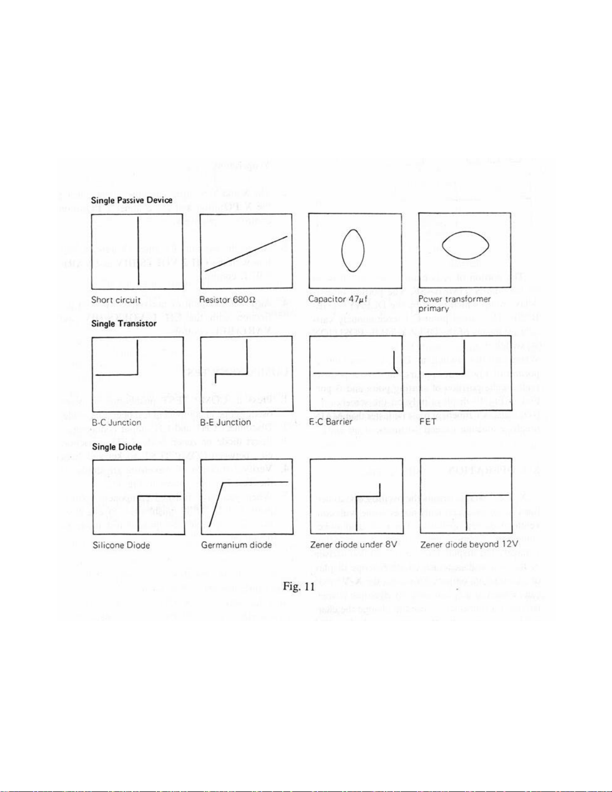
Para emplearlo, desconecte la puntas de prueba del osciloscopio, y presione el botón COMP TEST con lo que el instrumento estará listo para operar. Desconecte las puntas de prueba de los conectores de canal. A continuación, conecte el componente entre el terminal correspondiente marcado COMP TEST y GND. Verifique que la forma de onda obtenida se corresponde con las ilustradas en la fig. 11. Tenga en cuenta que para componentes similares pero de distintas características los graficos mostrarán posi blemente diferentes proporciones.

====================================================================

APLICACIONES

====================================================================

MEDICION DE TENSIONES DE CC (Todos los modelos)

Las técnicas que se describen a continuación pueden ser utilizadas para medición tanto de tensiones de CC puras ( sin superposición de otras señales ) , como de tensiones instantáneas en señales complejas.

1. Conecte la señal a medir y establezca una presentación adecuada, tal como para permitirle

observar los puntos de interés actuando sobre los atenuadores verticales y la base de tiempos. En estos casos, siempre los controles VARiables de los atenuadores verticales deben estar en posición CAL.

2. Lleva la llave COUPLING a AUTO y la Llave AC / GND / DC del canal en uso a GND. Establezca

un trazo horizontal que sirva de referencia. Puede modificar la posición mediante el control correspondiente, pero recuerde dejarlo en esa posición para la medición. Recuerde también la posición donde lo dejó, o use el trazo no utilizado como referencia.

3. Lleve la llave AC / GND / DC a DC y observe la señal. Si esto no es posible (queda fuera de

pantalla), repita los pasos anteriores hasta poder observarla en pantalla.

4. Con el control de posición horizontal, lleve la porción de señal a medir al centro de la pantalla,

haciéndola coincidir con las marcas verticales de la retícula.

5. Para medir el nivel de CC puede: contar las divisiones y fracciones entre la posición marcada

como referencia ( para asegurarse, lleve la llave AC / GND / DC a GND momentáneamente ) y el punto de interés, o bien si usa el Canal B, mover el control de posición hasta superponer el trazo con la referencia, y luego con el punto de interés, co ntando también las divisiones de retícula.

La tensión presente será

V CC = Nivel CC+ # Divisiones x VOLTS/DIV x Atenuación de la punta

Refiérase al ejemplo de la fig. 12. En todos los casos, trate que la cantidad de divisiones a contar sea de tres o m ás, para asegurar una

mejor precisión.

MEDICIÓN DE TENSIÓN ENTRE DOS PUNTOS DE UNA SEÑAL (Todos los modelos )

Este procedimiento puede utilizarse para medir tensiones pico a pico, tanto como para medir una diferencia de tensión entre dos puntos de una señal determinada.

Conecte la señal al instrumento, y mediante el atenuador ( siempre debe estar en CAL ), y la llave de base de tiempos logre una presentación tal que permita observar convenientemente los puntos de interés. Recuerde el uso de los controles de Nivel de Disparo, tanto como el de inhibición que permitirán una presentación estable.

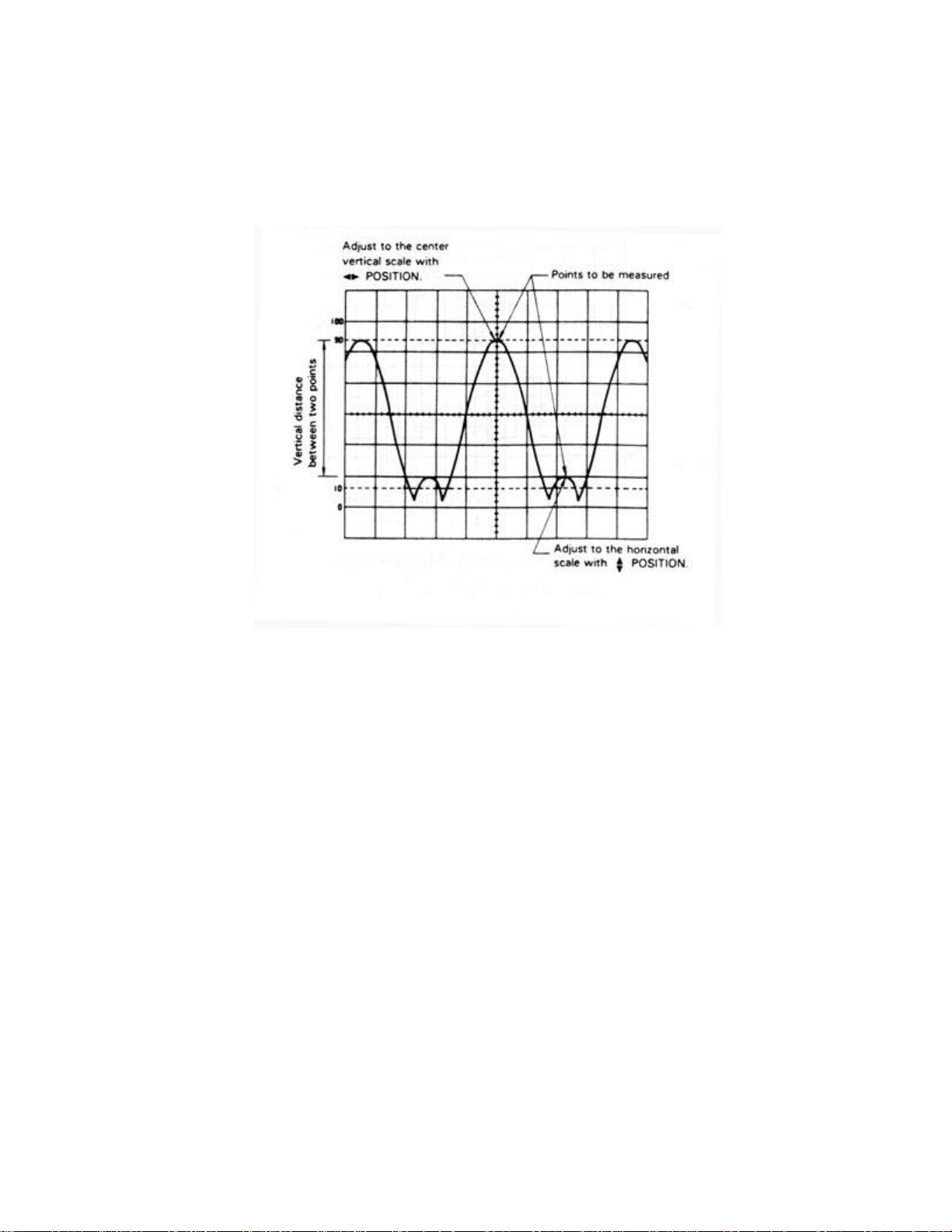
Usando el control de Posición vertical, ajuste la misma de modo que uno de los puntos de interés esté superpuesto a una de las divisiones mayores de la pantalla. Luego, con el control de posición horizontal desplace la imagen lateralmente, de modo de hacer coincidir el otro punto de interés por sobre la línea vertical de referencia. Léase cantidad de divisiones (enteras y fracciones) y multiplíquese este valor por el indicado por el atenuador vertical. Multiplíquese ahora por el factor de atenuación de la punta, y el resultado será la tensión medida entre dos puntos de la señal en cuestión.

MEDICIONES DE TIEMPO Y PERIODO (Todos los modelos )

Mediante este procedimiento se puede medir el período de una señal, y por consiguiente calcular la frecuencia de la misma. En señales digitales ( pulsos ), también se puede calcular el ciclo de actividad, así como el tiempo entre dos puntos de una misma señal.

Conecte la señal a medir a uno cualquiera de los canales verticales, y obtenga una presentación estable, de por lo menos un ciclo completo de la señal y de ser preferible algo más. Utilice el control

de HOLD OFF para conseguir una presentación estable. Asegúrese que el control VAR SWEEP este en CAL. Usando el control de posición horizontal desplace la imagen obtenida de modo que el punto elegido como inicio coincida con una división vertical. Al mismo tiempo, desplace la imagen verticalmente de modo que la línea de base coincida con línea horizontal graduada del centro de la pantalla. Mida la separación horizontal entre el punto elegido como inicio y el equivalente en el siguiente ciclo de la señal. Trate de obtener por lo menos 4 divisiones de separación para asegurar una mayor precisión. Tenga en cuenta si está habilitado el magnificador X 10.

El tiempo medido será entonces:

T = # Div. Horiz. x Tiempo / Div

ó T = # Div. Horiz. x Tiempo / Div x 10 si el magnificador x 10 está en uso. Véase el ejemplo de medición en pantalla y cálculo en la fig. 14

MEDICIONES DE FRECUENCIA (Todos los modelos )

El método es esencialmente similar a la medición de tiempos, con la excepción que en este caso se debe calcular luego la recíproca del período, es decir la frecuencia; para asegurar la mejor exactitud de la medición se debe tomar sea un período completo o semiperíodo en caso de señales de baja frecuencia, y en señales de alta frecuencia una cantidad entera de períodos, dividiendo luego o multiplicando por la cantidad de períodos medidos. En cualquier caso se debe trabajar con el control de VAR SWEEP en posición CAL. En el caso simple de un período o semiperíodo, se mide el tiempo, tal como en el método descrito anteriormente, y luego se calcula la inversa, obteniéndose la frecuencia. Véase el ejemplo de la fig. 15. En ese caso tenemos un ciclo completo de señal cuyo período es de 40 µs. El cálculo de frecuencia nos da entonces:

F = 1 / 40 x 10

-6

= 25 x 10 4 = 25 kHz. En el caso de señales de alta frecuencia, donde a lo mejor la velocidad de la base de tiempos no permite observar un único período se debe proceder como sigue:

1. Obtener, igual que para el caso anterior, una presentación estable en pantalla;

2. Ajustar con el control de posición horizontal para que el flanco ascendente de la señal coincida con

una marcación vertical en un período cualquiera. ;

3. Contar una cantidad N de períodos completos y determinar su duración, utilizando la línea

horizontal graduada de la retícula ( usar en lo posible cantidades enteras p. ej. 10 períodos y tener en cuenta si se usa o no el magnificador );

Efectuar luego el siguiente cálculo:

Numero de Períodos

f = -----------------------------------------

Tiempo Total

donde f = frecuencia de la señal; Tiempo total = cant. de divisiones x TIME / DIV Numero de períodos = cantidad de períodos de la señal observada. Refiérase a la fig. 16

MEDICIONES DE ANCHO DE PULSOS (Todos los modelos )

En este caso es conveniente que una vez se haya obtenido una presentación correcta, se desplace la señal en pantalla de forma que una división vertical coincida con el flanco ascendente de la señal a observar.

Obsérvese la fig. 17. El procedimiento consiste en utilizar una velocidad de barrido tal que se observe, de ser ello posible, solamente el pulso a medir ocupando el máximo espacio horizontal posible, y manteniendo el control VAR SWEEP en CAL. Es posible que sea necesario utilizar el HOLD OFF para obtener una imagen estable. Mídase entonces la longitud que ocupa el pulso y calcúlese la duración:

PW = N , M div x Y TIME / DIV x 1 / 10

NOTA : corresponde aplicar el factor 1 / 10 sólo si se usa el magnificador horizontal. N , M : divisiones enteras y su fracción Y es la velocidad de barrido en Unid. de tiempo por división.

TIEMPO DE ESTABLECIMIENTO Y DE CAIDA DE PULSOS (Todos los modelos)

En las mediciones de tiempo de establecimiento ( rise time ) y caida ( fall time ) de pulsos, se mide el tiempo transcurrido para una variación del 10 al 90 % en amplitud de la señal. Para lograr esto se debe seguir este procedimiento:

1. Conectar el osciloscopio a la señal a medir, y obtener una presentación estable, utilizando los

comandos de TRIGGER LEVEL, TIME / DIV y HOLD OFF.

2. Ajuste la amplitud de la señal con el control VOLTS / DIV y VAR de modo que esta ocupe

exactamente 6 divisiones verticales, y ajustando la velocidad de barrido a que la zona de interés ocupe el máximo ancho de pantalla.

3. Al hacer coincidir la señal con las 6 divisiones mencionadas antes, cerciórese que son las

marcadas 0 y 100 ( % ) en la retícula. Ahora se encontrará que la señal cruza una línea de trazos marcada 10 ( % ) y 90 ( % ) que son los puntos de interés.

4. Con el control de posición horizontal desplace el punto correspondiente al 10 % hacia una división

vertical mayor, y luego cuente el espacio en divisiones y fracciones, que multiplicado por la velocidad de barrido ( y eventualmente la magnificación x 10 ) darán el tiempo de establecimiento.

Rise time = # Div x TIME / DIV ( x 1 / 10 )

NOTA : corresponde aplicar el factor 1 / 10 sólo si se usa el magnificador horizontal. De la misma manera se puede medir el tiempo de caida, seleccionando el flanco descendente de la señal.

DIFERENCIAS DE TIEMPO Y / O FASE ENTRE SEÑALES (Todos los modelos )

Esta medición permite determinar la diferencia de tiempo entre dos señales relacionadas y sincronizadas entre sí, que presentan una diferencia de tiempo entre la ocurrencia de cada una de ellas.

Aplique las señales a analizar a los canales verticales y obtenga una presentación estable con los controles de barrido. Recuerde elegir el modo vertical adecuadamente ( CHOP ) para evitar introducir una diferencia de fase adicional a la señal.

Seleccione la de mayor frecuencia para el disparo.

Actúe con los controles de posición vertical de modo que ambas ocupen el centro de la pantalla en sentido vertical.

Actúe sobre la posición horizontal, de modo de hacer coincidir una de las dos señales (la de referencia) con una división vertical cualquiera.

Mida ahora la diferencia de tiempo contando las divisiones y fracción sobre la línea central. Tenga en cuenta si está en uso el magnificador.

El cálculo es:

∆ Τ = # Div. x TIME / DIV ( x 1 / 10 )

NOTA : corresponde aplicar el factor 1 / 10 sólo si se usa el magnificador horizontal. Véase como referencia la fig. 19.

Fig. 19

MEDICION DE DIFERENCIA DE FASE (Todos los modelos )

Uno de los métodos disponibles ha sido descrito en el párrafo anterior, y es utilizable en la medida que se pueda establecer una presentación estable, es decir sin oscilaciones de posición horizontal (jitter).

Dado que ambas señales son afectadas por igual por las condiciones del barrido, la diferencia de fase será irrespectiva de estos. Teniendo este valor en cuenta, es fácil determinar la diferencia de fase mediante un simple cálculo:

∆ ϕ = 360° / # Div x N, M Div ( x 1 / 10 )

donde

∆ ϕ = diferencia de fase en grados;

# Div = numero de divisiones ocupado por un ciclo;

N , M = numero de divisiones enteras y fracciones;

1 / 10 = factor de magnificación. Recuerde que sea como sea se debe mantener una presentación estable, por lo que puede ser

necesario actuar sobre los controles de tanto en tanto, excepto del de VAR.

MEDICION DE TENSIONES DE CC Y TENSIÓN ENTRE DOS PUNTOS DE UNA SEÑAL

Para ambos casos, ubíquese el cursor de referencia ( X ) en un punto apropiado de la señal a medir. Presione ahora " SEL " para seleccionar el otro cursor. Con los botones de desplazamiento posicione el cursor " + " en el punto que se desee medir, y léanse los valores obtenidos en el ángulo superior izquierdo de la pantalla. En el ejemplo de la figura, se tiene una sensibilidad de 200 mV/div., y el resultado de la medición se observa en el angulo sup. izquierdo, así como la diiferencia de tiempo entre cursores (en este caso

corresponde al período de la señal.

MEDICIONES DE TIEMPO Y PERIODO - MEDICIONES DE FRECUENCIA - MEDICIONES DE ANCHO DE PULSOS

Para estas tres mediciones, se debe posicionar el cursor de referencia ( X ) en un punto apropiado de la señal mediante los botones de desplazamiento. Presione ahora " SEL " para seleccionar el otro cursor. Con los botones de desplazamiento posicione el cursor " + " en el punto que se desee medir, y léanse los valores obtenidos en el ángulo superior derecho de la pantalla. En este caso, es posible leer valores de tiempo en forma directa, o de frecuencia, presionando el botón 1 / ∆ Τ

TIEMPO DE ESTABLECIMIENTO Y DE CAIDA DE PULSOS

En las mediciones de tiempo de establecimiento ( rise time ) y caida ( fall time ) de pulsos, se mide el tiempo transcurrido para una variación del 10 al 90 % en la amplitud de la señal. Para lograr esto con el RS 608 se debe seguir este procedimiento:

• Conectar el osciloscopio a la señal a medir, y obtener una presentación estable, utilizando los

comandos de TRIGGER LEVEL, TIME / DIV y HOLD OFF.

• Ajuste la amplitud de la señal con el control VOLTS / DIV y VAR de modo que esta ocupe

exactamente 6 divisiones vertic ales, y ajustando la velocidad de barrido a que la zona de interés ocupe el máximo ancho de pantalla.

• Al hacer coincidir la señal con las 6 divisiones mencionadas antes, cerciórese que son las

marcadas 0 y 100 ( % ) en la retícula. Ahora se encontrará que la señal cruza una línea de trazos marcada 10 ( % ) y 90 ( % ) que son los puntos de interés.

• Con los botones de desplazamiento posicione el cursor de referencia ( X ) sobre el punto donde la

señal intersecta la marca de 10 % .

• Presione SEL seleccionando el cursor " + "

• Desplace este cursor hacia el punto donde la señal intersecta la marca del 90 %

• Lea el valor de tiempo en el ángulo superior derecho de la pantalla.

De la misma manera se puede medir el tiempo de caida, seleccionando el flanco descendente de la señal.

DIFERENCIAS DE TIEMPO Y / O FASE ENTRE SEÑALES - MEDICION DE DIFERENCIA DE FASE

Uno de los métodos disponibles ha sido descrito anteriormente y es válido, pero , y es utilizable en la medida que se pueda establecer una presentación estable, es decir sin oscilaciones de posición horizontal (jitter).

Otro de los métodos disponibles es generar una presentación, mediante la actuación adecuada de los controles de barrido ( TIME / DIV; HOLD OFF; VAR; POS) tal que un ciclo completo de la señal de referencia ocupe un espacio definido en pantalla, p. ej. 10 divisiones. De esta manera, cada división representa 360 ° / 10 = 36 °. Dado que ambas señales son afectadas por igual por las condiciones del barrido, la diferencia de fase será irrespectiva de estos. Teniendo este valor en cuenta, es fácil determinar la diferencia de fase mediante un simple cálculo:

∆ ϕ = 360° / # Div x N, M Div ( x 1 / 10 )

donde

∆ ϕ = diferencia de fase en grados;

# Div = numero de divisiones ocupado por un ciclo;

N , M = numero de divisiones enteras y fracciones;

1 / 10 = factor de magnificación. Recuerde que sea como sea se debe mantener una presentación estable, por lo que puede ser

necesario actuar sobre los controles de tanto en tanto, excepto del de VAR.

APLICACIONES EN MODO X-Y

Este modo es particularmente útil en el análisis de frecuencias de audio, y mediante un método simple permite determinar relaciones de fase y distorsión en amplificadores.

Se debe poseer un generador de audio, preferentemente de baja distorsión armónica, y eventualmente para análisis de respuesta en frecuencia un generador de funciones o un generador de audio con barrido. Siga el siguiente procedimiento para analizar un amplificador:

1. Conecte un generador de audio al amplificador o circuito bajo ensayo;

2. Ajústelo para niveles normales de operación;

3. Conecte el canal B a la entrada del amplificador, en paralelo con ésta y el canal A a la salida del

mismo. Verifique que no exista sobreexcitación y recorte de señal, y ajuste el osciloscopio de modo de obtener la misma amplitud en pantalla, en modo normal.

4. Seleccione operación en X-Y con el botón.

5. Verifique la condición del amplificador, comparando la imagen obtenida con las ilustradas en la fig. Típicamente, dos señales en fase producen una línea recta a 45°; dos señales fuera de fase, una elipse, dos señales separadas por 90 ° una circunferencia. La distorsión se indica como un achatamiento en algún lugar de la elipse o circunferencia obtenida. La diferencia de fase se puede calcular también.

Medición de Respuesta en frecuencia

Para esto se debe disponer de un generador de barrido de audio, o un generador de funciones con barrido y un rango de por lo menos de 1000:1 para cubrir el rango audible ( 20 Hz a 20.000 Hz ), y efectuar el siguiente procedimiento. Conecte la señal de diente de sierra del barredor al canal A del osciloscopio. Con el barrido activado, haga que este cubra el ancho total de pantalla, p. ej. 10 div horizontales. Conecte un demodulador a la salida del circuito a ensayar, y la salida de CC del demodulador a la entrada del canal B del osciloscopio. Ajuste la amplitud del canal B de forma que puedan usarse las marcas de referencia de la retícula para comparar amplificación, atenuación, etc.

MANTENIMIENTO

La serie de osciloscopios B&K PRECISION PS requiere poco o nulo mantenimiento por parte del usuario, mientras que el equipo sea operado dentro de sus características. Las instrucciones siguientes están prevista para ser ejecutadas por personal técnicamente competente y adiestrado en el manejo y eventual reparación de instrumental. Si no está familiarizado con el equipo, no intente reemplazar componentes internos o efectuar modificaciones. Recurra al repreentante de quie obtuvo el instrumento.

Dentro de las tareas periódicas a realizar se encuentran la compensación de las puntas de prueba, y la rotación de trazo .

La compensación de las puntas de prueba se debe realizar cada vez que se reemplaza la punta por una nueva, o se utiliza la de un canal en el otro. Esto es por que si bien se toma el máximo cuidado en la selección de componentes, existe siempre una pequeña diferencia entre ellos por lo cual se deberá efectuar el ajuste manual.

El procedimiento es como sigue:

• Conecte una punta a Canal 1 y la otra a Canal 2. En lo posible identifíquelas de modo de evitar el

intercambio.

• Con una de la puntas toque el terminal marcado CAL en el frente del instrumento.

• Ajuste el atenuador para ver una señal de 5 o 6 div de altura y por lo menos 3 o cuatro ciclos

completos de ella.

• Ajuste el capacitor de compensación ubicado, (según el modelo de punta suministrado) en:

A - El conjunto conector BNC / circuito compensador.

B – Cuerpo de la punta, cerca del selector de atenuación. La figura muestra la respuesta de una punta compensa da correctamente (trazo superior), con exceso

y con falta de compensación en los siguientes trazos. Utilice siempre que sea posible un calibrador cerámico; de no serlo, utilice un destornillador pequeño

de mango aislado con la hoja más corta posible. En ambos casos tenga extremo cuidado de no dañar al capacitor; pues esto obligará al reemplazo de la punta completa.

Para efectuar la rotación de trazo , debe primero colocar el osciloscopio en su ubicación definitiva. Una vez hecho esto, proceda como sigue:

Encienda el instrumento y coloque el selector COUPLING de la Base de tiempos en AUTO. Observe que se produzca una trazo mas o menos horizontal.

Centre este trazo en la pantalla con los controles de posición, usando como guía el eje horizontal mayor del TRC. Con un destornillador pequeño, ajuste el control TRACE ROTATION ubicado en el panel frontal, entre los controles de intensidad ( INTENSITY ) y foco ( FOCUS ) hasta lograr un paralelismo perfecto entre el trazo y la linea de referencia. Tenga cuidado c on la herramienta usada, pues el eje del control es de material plástico, por lo que puede dañarse de no ser tratado adecuadamente. DE ser posible use un calibrador cerámico.

Reemplazo de fusibles.

Esta tarea debe ser efectuada solamente ante un cambio de la tensión de alimentación, o cuando el fusible se ha quemado. Si es válido el último caso, debe investigarse la causa. Reemplace el fusible, y si nuevamente se quema, recurra a su distribuidor, o a personal especializado y debidamente capacitado para investigar las causas y proceder a una reparación. No reemplace el fusible por otro de mayor

capacidad. Puede dañar al instrumento.

En caso de cambios en la alimentación, reemplace el fusible según el siguiente detalle:

115 V 800 mA @ 250 V 230 V 600 mA @ 250 V

El fusible va alojado dentro del selector de tensión ubicado en el panel trasero.

Verificación de calibración

Todos los instrumentos de la serie PS están provistos de un terminal marcado CAL que entrega una señal rectangular de 2 V p-p +/-3% que es normalmente suficiente para verificaciones periódicas. Téngase en cuenta que es solamente para una verificación rápida de la validez de las indicaciones del instrumento y atenuación de las puntas de prueba. Peródicamente conecte la punta a la señal de calibración y verifique que en todas las posiciones del atenuador, se mantenga la calibración del instrumento. Efectúe esta verificación siempre en los dos canales. En caso de anomalías, diríjase a su distribuidor y no intente efectuar reparación alguna.

Información de Servicio

Servicio de Garantía: Por favor regrese el producto en el empaquetado original con prueba de la fecha de la compra a la dirección debajo. Indique claramente el problema en escritura, incluya todos los accesorios que se estan usado con el equipo.

Servicio de No Garantía: Por favor regrese el producto en el empaquetado original con prueba de la fecha de la compra a la dirección debajo. Indique claramente el problema en escritura, incluya todos los accesorios que se estan usado con el equipo. Clientes que no tienen cuentas deben de incluir pago en forma de queque, orden de dinero, o numero de carta de crédito. Para los precisos mas corriente visite www.bkprecision.com y oprime “service/repair”.

Vuelva toda la mercancía a B&K Precision Corp. con el envío pagado por adelantado. La carga global de la reparación para el servicio de la No-Garantía no incluye el envío de vuelta. El envío de vuelta a las localizaciones en norte americano es incluido para el servicio de la garantía. Para los envíos de noche y el envío del no-Norte los honorarios americanos satisfacen el contacto B&K Precision Corp.

B&K Precision Corp. 22820 Savi Ranch Parkway Yorba Linda, CA 92887 www.bkprecision.com 714-921-9095

Incluya con el instrumento la dirección de vuelto para envío, nombre del contacto, número de teléfono y descripción del problema.

Garantía Limitada de Tres Anos

B&K Precision Corp. Autorizaciones al comprador original que su productos y componentes serán libre de defectos por el periodo de tres anos desde el día en que se compro.

B&K Precision Corp. sin carga, repararemos o sustituir, a nuestra opción, producto defectivo o componentes. Producto devuelto tiene que ser acompañado con prueba de la fecha del la compra en la forma de tres recibo de las ventas.

Para obtener cobertura en los EE.UU., este producto debe ser registrado por medio de la forma de registro en

www.bkprecision.com dentro de quince (15) días de la compra de este producto.

Exclusiones: Esta garantía no se aplica en el evento de uso en error o abuso de este producto o el resultado de alteraciones desautorizado o reparaciones. La garantía es vacía si se altera, se desfigura o se quita el número de serie.

B&K Precision Corp. no será obligado a dar servicio por danoss consecuente, incluyendo sin limitaciones a danoss resultando en perdida de uso. Algtresos estados no permiten limitaciones de daños fortuitos o consecuentes. Tan la limitación o la exclusión antedicha puede no aplicarse a usted.

Esta garantía le da ciertos derechos y pueden tener otros derechos, cuales camb ian estado por estado.

B&K Precision Corp. 22820 Savi Ranch Parkway Yorba Linda, CA 92887 www.bkprecision.com 714-921-9095

INFORMATION

One of the best tutorials on oscilloscopes in the industry. Valuable to those with little knowledge

of oscilloscopes as well as the experienced technician or engineer who wishes

to refresh their memory or explore new uses for oscilloscopes.

Download your FREE copy

from our Web site

www.bkprecision.com

Declaration of CE Conformity

according to EEC directives and NF EN 45014 norm

Responsible Party

Manufacturer’s Name: B&K Precision Corporation

Manufacture’s Address: 22820 Savi Ranch Pkwy.

Yorba Linda, CA 92887-4610 USA

Declares that the below mentioned product

Product Name: Oscilloscope

Part Numbers: 1541D, 2120B, 2125A, 2160A, 2522B

complies with the essential requirements of the following applicable European Directives:

Low Voltage Directive 73/23/EEC (19.02.73) amended by 93/68/EEC (22.07.93) Electromagnetic Compatibility (EMC) 89/336/EEC (03.05.88) amended by 92/68/EEC (22.07.93)

and conforms with the following product standards:

LV D EN 61010-1

EMC EN 50081-1 -- EN 55022

EN 60555-2

EN 50082-1 -- IEC 801-2

IEC 801-3 IEC 801-4

This Declaration of Conformity applies to above listed products place on the EU market after:

January 1, 2005

Date Victor Tolan

President

22820 Savi Ranch Parkway, Yorba Linda, CA 92887

481-313-9-001 Printed in Taiwan

BK Precision 2160A, 1541D User Manual

Specifications and Main Features

Frequently Asked Questions

User Manual