

organic compounds per unit time
are purposely produced in order to
be screened against a variety of biological targets for drug detection.
Introduction
High sample throughput is particularly important in the pharmaceutical industry, for example, in
combinatorial chemistry and
metabolite studies. In combinatorial chemistry a large number of
An ideal instrument configuration
for high sample throughput comprises:
• an autosampler such as a standard HPLC autosampler for
2-ml vials or a sampler with
microtiter and deep-well plates,
• a high-pressure gradient pump
for lowest delay volume,
• a UV detector such as a diode
array detector or variable wavelength detector, and
• a mass selective detector for
additional mass and structural
information (optional).
Optimizing the Agilent 1100 Series
System for High Sample Throughput
Technical Note
Agilent Technologies
Innovating the HP Way

The limiting factor for high
throughput in such systems is the
speed of the HPLC analysis.
Standard HPLC cycle times from
injection to injection for gradient
analysis lie between 15 and 20 min
using columns of 100 to 200 mm in
length.
To significantly increase the sample throughput, cycle times must
be shortened. This can be
achieved using fast gradients with
short columns and high flow rates.
In the following example we
demonstrate how to optimize the
Agilent 1100 Series high-pressure
gradient system to obtain rapid
gradients and high sample
throughput. Hints are given on the
influence of chromatographic
parameters on cycle times, and on
how run times of less than two
minutes can be expected to affect
performance.
Equipment
All HPLC experiments were carried out on the Agilent 1100 Series
high-pressure gradient system
comprising:
• Agilent 1100 Series high-pressure
pump for lowest delay volume.
In this design each solvent is
pumped by its own pump
assembly, and mixing takes
place on the high-pressure side.
This means gradient changes
reach the column much faster
than in low-pressure gradient
systems where mixing takes
place on the low-pressure side.
• Agilent 1100 Series vacuum
degasser for optimum baseline
stability.
• Agilent 1100 Series autosampler
for sampling from 2-ml standard
vials.
• Optional Agilent 220 micro
plate sampler for flexible sampling from deepwell and/or
microtiter plates.
• Agilent 1100 Series thermostatted column compartment for
highest stability from 10 °C
below ambient up to 80 °C.
• Agilent 1100 Series diode array
detector with standard flow cell
(10-mm pathlength, 13-microliter volume).
• Optional Agilent 1100 Series
variable wavelength detector.
• Optional Agilent 1100 Series
LC/MSD module for mass and
structural information.
• Agilent ChemStation with 3D
HPLC single instrument software
for instrument control, data handling and sample tracking.
Compounds and chromatographic conditions
For our experiments we selected
the following compounds which
differ considerably in polarity:
• caffeine
• primidone
• phenacetin
• mandelic acid benzylester
• biphenyl
The chromatographic conditions
are listed next to the figures.
Optimization of chromatographic parameters
The following parameters have to
be adapted to obtain short cycle
times, sufficient resolution and
best performance over a wide
range of polarity:
• column length
• gradient
• flow rate
• delay volume
• data rate of detector
• column temperature
The aim was to achieve cycle
times of about 2 min and baseline
separation for all compounds.
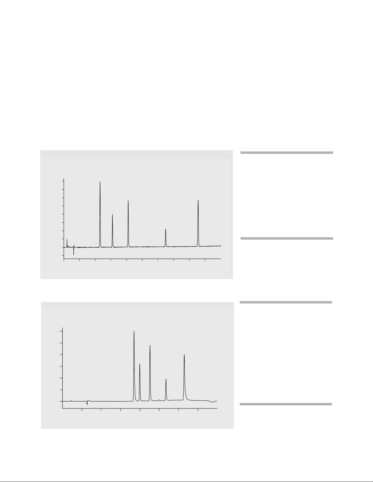
Influence of column length on
run time
For a standard column with a
length of 100 mm and an id of
4.6 mm, run time cycles of about
15 min are good practice. In
figure 1, the compounds mentioned in the previous paragraph
were analyzed.
Cycle times of 14 min were
obtained with excellent resolution
for all compounds.
Shorter cycle times are obtained
using a short column. In figure 2,
the analysis of the same compounds is shown using a 50-mm
colum. Cycle times are down to
2.8 min and baseline separation
for all compounds is given, despite
decrease in resolution. Shortening
the column length was the principal step in achieving reduced
cycle times. The example on the
next page demonstrates how to
shorten the cycle even further.
Column 100 x 4.6 mm ODS
Hypersil, 5 µm
Flow rate 2 ml/min
Mobile phase A = water, B = ace-
tonitrile (ACN)
Gradient 5 % B to 95 % B in
12 min
to 5 % B in 13 min
Run time 13 min
Post run 1 min
Diode-array settings 210/8 nm,
ref. wavelength
360/100 nm
Injector volume 5 µl
Column temperature 50 °C
Figure 1
Analysis of selected compounds using a 100-mm column
Figure 2
Analysis of selected compounds using a 50-mm column
Column 50 x 4.6 mm Zorbax
SB-C18, 3.5 µm
Flow rate 2 ml/min
Mobile phase A = water, B = ace-
tonitrile (ACN)
Gradient 5 % B to 95 % B in
1 min
95 % up to 1.5 min
to 5 % B in min
Run time 2 min
Post run 0.8 min
Diode-array settings 210/8 nm,
ref. wavelength
360/100 nm,
response time 0.1 s
Injector volume 5 µl, autosampler in
bypass mode
Column temperature 50 °C
Absorbance
[mAU]
400
350
300
250
200
150
100
50
0
-50
0
Absorbance
[mAU]
1200
1000
800
600
400
200
0
1
2
3
2
1
1 Caffeine 4 Mandelic acid
2 Primidone benzylester
3 Phenacetin 5 Biphenyl
3
5
4
Time [min]
5
4
9
8
7
6
0.25
0.5
0.75
1
Time [min]
1.25
1.5
1.75

Influence of gradient on run
time
In order to achieve a good separation for the polar and the nonpolar compounds, a gradient from
5 to 95 % of the organic phase was
chosen. The evaluation of the
steepest possible gradient with
baseline separation for all compounds is shown in figure 3. The
flow rate was 2 ml/min.
As a result, the gradient from 5 to
95 % ACN in 1 min met the
demands of shortest run time and
baseline separation for all peaks.
Influence of flow rate on run
time
As well as the column length, the
flow rate can also be used to
shorten run times or achieve better cycle times. In figure 4, the
analysis of the selected compounds at 4 different flow rates is
shown using the gradient from
5 to 95 % ACN in 1 min.
Cycle time can be reduced from
3 min at a 1 ml/min flow rate,
down to 1.3 min at a flow rate of
4 ml/min. All peaks are baseline
separated, also at a flow rate of
4 ml/min. In the evaluation of peak
area counts, it is apparent that
there are about four times less
area counts in the 4-ml/min run
than in the 1-ml/min run.
Figure 3
Evaluation of gradient steepness
Figure 4
Analysis of selected compounds at four different flow rates
Absorbance
[mAU]
800
400
0
800
400
0
1200
800
400
0
0.5
0.5
0.5
5 % to 95 ACN in
1
1
1
1.5
1.5
1.5
Time [min]
2
2
2
2.5
5 % to 95 ACN in
2.5
5 % to 95 ACN in
2.5
3 min
3
2 min
3
1 min
3
Absorbance
[mAU]
1500
0
1000
0
800
0
600
0
0
0
0
0
1 ml/min
0.25
2 ml/min
0.25
3 ml/min
0.25
4 ml/min
0.25
0.5
0.5
0.5
0.5
0.75
0.75
0.75
0.75
1
1
1
1
Time [min]
1.25
1.25
1.25
1.25
1.5
1.5
1.75
2

Influence of high flow rates on
minimum detectable concentrations
If a high flow rate is run, peak
heights and area counts for UV
detection are reduced. Consequently, for UV detectors, which
are able to detect compounds in
the 0.1 ppm range, the compound
concentration in the analyzed
sample should be in the low ppm
or high ppt range to ensure that
the UV detector is able to “see”
the compounds. It must also be
taken into account that a mass
selective detector (MSD) cannot
handle flow rates of 4 ml/min. The
maximum flow rate range is about
1 to 1.5 ml/min. Optimum flow
rates for most MSD instruments
are about 0.5 ml/min. The column
eluent must therefore be split 1 to
10 for optimum conditions. The
MSD is able to detect masses in
the 100 ppt range. If the compound concentration of the evaluated sample is in the low ppb
range, the MSD should still be able
to detect the masses, even though
the column eluent has to be split
before entering the ion source.
Influence of delay volume on
run time
Modern high-pressure gradient systems, such as the Agilent 1100
Series, offer system delay volume
below 1 ml without modifying the
standard system. The Agilent 1100
Series also offers the possibility to
switch the Agilent 1100 Series
autosampler into bypass mode
after the sample has reached the
column. This is done using an
injector program saving another
300 µl of delay volume. In figure 5,
the effect when switching the
autosampler into bypass mode is
shown. The experiment was done
at a flow rate of 2 ml/min, with a
gradient of 5 to 95 % ACN in 1 min.
The following injector program
used was used:
1. DRAW 5 µl from sample
2. INJECT
3. WAIT 0.03 min
4. VALVE bypass
5. WAIT 1.75 min
6. VALVE mainpass
The wait time before the valve is
switched to the bypass position
depends on the injection volume,
according to the equation:
Wait time = 6 (injection volume +
5 µl)/flow rate.
The run time difference for the
last peak is about 0.16 min which
corresponds to a volume of 320 µl
at 2 ml/min. The influence of the
delay volume is not significant in
this case and the higher the flow
rate the lower the gain in time.
Influence of data rate on precision
Assuming that 20 to 30 data points
per peak are needed for a precise
measurement, the set data rate of
a response time of 0.1 s is sufficient for a peak width of 2 s. The
peak width is measured at peak
bottom (4 s). This peak width produces 20 data points. All peaks,
even those measured at a flow
rate of 4 ml/min, are broad enough
to produce at least 20 data points
per peak.
Influence of column temperature on run time
The influence of column temperature was tested for 50 °C and
25 °C at a 2 ml/ min flow rate,
using the gradient from 5 to 95 %
ACN in 1 min. The influence is low
in this case. The retention time
difference for the last peak is only
0.052 min.
Figure 5
Analysis of selected compounds at different delay volumes
Absorbance
[mAU]
1200
Agilent 1100 Series
800
autosampler in bypass mode
400
0
0.8
0.6
0.4
0.2
1200
Agilent 1100 Series
800
autosampler in mainpass mode
400
0
0.8
0.6
0.4
0.2
1.8
1.6
1.4
1.2
1
1.8
1.6
1.4
1.2
1
Time [min]

Results of optimization
process
The aim was to obtain cycle times
of about 2 min and baseline separation of all analyzed compounds.
This was achieved as shown in
figure 6.
The time the autosampler needs to
inject the next sample is sufficient
to equilibrate the system for the
start conditions.
Method performance was tested
over 10 runs and relative standard
deviations (rsd) are listed in
table 1. The injection volume was
5 µl. The precision of areas is
worse than normally expected in
HPLC. This is due to the low number of data points that can be
acquired at such narrow peak
width.
Compared to standard cycle times
of about 15 to 20 min, the cycle
time could be reduced by a factor
of 10.
Figure 6
Optimized chromatogram for high throughput and cycle run times below 1.5 min
Compound Precision of retention time Precision of areas
Caffeine 0.30 2.60
Primidone 0.29 2.58
Phenacetin 0.19 2.51
Madelic acid benylester 0.16 2.58
Biphenyl 0.06 2.32
Table 1
Precision of rentention times and areas
Column 50 x 4.6 mm Zorbax
SB-C18, 3.5 µm
Flow rate 4 ml/min
Mobile phase A = water, B = ace-
tonitrile (ACN)
Gradient 5 % B to 95 % B in
1 min,
95 % until 1.09 min
to 5 % B at 1.1 min
Run time 1.2 min
Post run time needed to inject
the next sample
Diode-array settings 210/8 nm,
ref. wavelength
360/100 nm,
response time 0.1 s
Injector volume 5 µl, autosampler in
bypass mode
Column temperature 50 °C
Absorbance
[mAU]
800
600
400
200
0
0
0.25
0.5
Time [min]
0.75
1

Conclusions
High-sample throughput in an
HPLC system can be achieved by
optimizing the cycle times from
injection to injection using short
columns, high flow rates and steep
gradients. Such an HPLC system
should include a high-pressure
gradient pump. These pumps have
low delay volumes and gradient
changes almost immediately affect
the column. The column length
should be 50 mm or less, and the
internal diameter should be
approximately 4.6 mm. Start and
end concentration of the gradient
composition should be selected
such that it has an impact on all
compounds. Otherwise the unaffected compounds tend to
broaden, especially at higher injection volumes. The gradient slope
should be as steep as possible,
however, peak resolution is the
limiting factor. A high flow rate of
approximately 2 to 4 ml/min is
recommended in order to further
reduce run times and equilibration
times. The data rate must be set as
high as possible to guarantee at
least 20 to 30 data points per peak.
If all parameters are optimized,
the sample throughput can be
increased at least by a factor of 10
with good precision for retention
times and areas.
Literature Reference
Wolfgang K. Goetzinger and
James N.Kyranos, “Fast gradient
RP-HPLC for high throughput
quality control analysis of spatially
addressable combinatorial
libraries” American Laboratory,
pp 27-37, April 1998.

For the latest information and services visit
our world wide web site:
http://www.agilent.com/chem
Agilent Technologies
Innovating the HP Way
Copyright © 1998 Agilent Technologies
All Rights Reserved. Reproduction, adaptation
or translation without prior written permission
is prohibited, except as allowed under the
copyright laws.
Publication Number 5968-0467E
 Loading...