

Page 1

CAS
Reference Guide
This guidebook applies to TI-Nspire™ software version 1.4. To obtain the
latest version of the documentation, go to education.ti.com/guides.
Page 2

Important Information
Except as otherwise expressly stated in the License that accompanies a
program, Texas Instruments makes no warranty, either express or
implied, including but not limited to any implied warranties of
merchantability and fitness for a particular purpose, regarding any
programs or book materials and makes such materials available solely on
an "as-is" basis. In no event shall Texas Instruments be liable to anyone
for special, collateral, incidental, or consequential damages in connection
with or arising out of the purchase or use of these materials, and the sole
and exclusive liability of Texas Instruments, regardless of the form of
action, shall not exceed the amount set forth in the license for the
program. Moreover, Texas Instruments shall not be liable for any claim of
any kind whatsoever against the use of these materials by any other
party.
License
Please see the complete license installed in C:\Program Files\TI
Education\TI-Nspire CAS.
© 2008 Texas Instruments Incorporated
Macintosh®, Windows®, Excel®, Vernier EasyLink®, EasyTemp®,
Go!®Link, Go!®Motion, and Go!®Temp are trademarks of their
respective owners.
ii
Page 3

Contents
Expression templates
Fraction template ........................................ 1
Exponent template ......................................1
Square root template .................................. 1
Nth root template ........................................1
e exponent template ................................... 2
Log template ................................................ 2
Piecewise template (2-piece) .......................2
Piecewise template (N-piece) ......................2
System of 2 equations template ................. 3
System of N equations template .................3
Absolute value template .............................3
dd°mm’ss.ss’’ template ................................3
Matrix template (2 x 2) ................................3
Matrix template (1 x 2) ................................4
Matrix template (2 x 1) ................................4
Matrix template (m x n) .............................. 4
Sum template (G) ......................................... 4
Product template (Π) ...................................4
First derivative template ............................. 5
Nth derivative template .............................. 5
Definite integral template ..........................5
indefinite integral template ....................... 5
Limit template .............................................. 5
Alphabetical listing
A
abs() ..............................................................6
amortTbl() .................................................... 6
and ................................................................6
angle() ..........................................................7
ANOVA .........................................................7
ANOVA2way ................................................ 8
Ans ..............................................................10
approx() ......................................................10
approxRational() ........................................ 10
arcLen() .......................................................10
augment() ...................................................10
avgRC() ....................................................... 11
B
bal() .............................................................11
4Base2 .........................................................12
4Base10 .......................................................12
4Base16 .......................................................12
binomCdf() ................................................. 13
binomPdf() ................................................. 13
C
ceiling() .......................................................13
cFactor() ......................................................13
char() ...........................................................14
charPoly() ....................................................14
2
c
2way ........................................................14
2
Cdf() .........................................................15
c
2
GOF ......................................................... 15
c
2
Pdf() .........................................................15
c
ClearAZ .......................................................16
ClrErr .......................................................... 16
colAugment() ............................................. 16
colDim() ...................................................... 16
colNorm() ................................................... 16
comDenom() .............................................. 17
conj() .......................................................... 17
constructMat() ........................................... 18
CopyVar ...................................................... 18
corrMat() .................................................... 18
4cos ............................................................. 19
cos() ............................................................ 19
cosê() .......................................................... 20
cosh() .......................................................... 21
coshê() ........................................................ 21
cot() ............................................................ 21
cotê() .......................................................... 22
coth() .......................................................... 22
cothê() ........................................................ 22
count() ........................................................ 22
countif() ..................................................... 23
crossP() ....................................................... 23
csc() ............................................................. 23
cscê() ........................................................... 24
csch() ........................................................... 24
cschê() ......................................................... 24
cSolve() ....................................................... 24
CubicReg .................................................... 26
cumSum() ................................................... 27
Cycle ........................................................... 27
4Cylind ........................................................ 27
cZeros() ....................................................... 27
D
dbd() ........................................................... 29
4DD ............................................................. 29
4Decimal ..................................................... 30
Define ......................................................... 30
Define LibPriv ............................................ 31
Define LibPub ............................................ 31
DelVar ........................................................ 31
deSolve() .................................................... 32
det() ............................................................ 33
diag() .......................................................... 33
dim() ........................................................... 33
Disp ............................................................. 34
4DMS ........................................................... 34
dominantTerm() ........................................ 35
dotP() .......................................................... 35
E
e^() ............................................................. 36
eff() ............................................................. 36
eigVc() ........................................................ 36
eigVl() ......................................................... 37
Else ............................................................. 37
ElseIf ........................................................... 37
EndFor ........................................................ 37
EndFunc ...................................................... 37
EndIf ........................................................... 37
EndLoop ..................................................... 37
iii
Page 4

EndPrgm .....................................................37
EndTry .........................................................37
EndWhile ....................................................38
exact() .........................................................38
Exit ..............................................................38
4exp .............................................................38
exp() ............................................................38
exp4list() ......................................................39
expand() ......................................................39
expr() ...........................................................40
ExpReg ........................................................40
F
factor() ........................................................41
FCdf() ..........................................................42
Fill ................................................................42
FiveNumSummary ......................................42
floor() ..........................................................43
fMax() .........................................................43
fMin() ..........................................................43
For ...............................................................44
format() ......................................................44
fPart() ..........................................................44
FPdf() ..........................................................44
freqTable4list() ............................................45
frequency() .................................................45
FTest_2Samp ..............................................45
Func .............................................................46
G
gcd() ............................................................46
geomCdf() ...................................................46
geomPdf() ...................................................47
getDenom() ................................................47
getLangInfo() .............................................47
getMode() ...................................................47
getNum() ....................................................48
getVarInfo() ................................................48
Goto ............................................................49
4Grad ...........................................................49
I
identity() .....................................................50
If ..................................................................50
ifFn() ............................................................51
imag() ..........................................................51
impDif() .......................................................52
Indirection ..................................................52
inString() .....................................................52
int() .............................................................52
intDiv() ........................................................52
integrate .....................................................52
2
() .........................................................53
invc
invF() ...........................................................53
invNorm() ....................................................53
invt() ............................................................53
iPart() ..........................................................53
irr() ..............................................................53
isPrime() ......................................................54
L
Lbl ...............................................................54
lcm() ............................................................54
left() ............................................................ 55
libShortcut() ............................................... 55
limit() or lim() ............................................. 55
LinRegBx ..................................................... 56
LinRegMx ................................................... 57
LinRegtIntervals ......................................... 57
LinRegtTest ................................................ 59
@List() .......................................................... 59
list4mat() ..................................................... 60
4ln ................................................................ 60
ln() .............................................................. 60
LnReg .......................................................... 61
Local ........................................................... 61
log() ............................................................ 62
4logbase ...................................................... 62
Logistic ....................................................... 63
LogisticD ..................................................... 63
Loop ............................................................ 64
LU ................................................................ 65
M
mat4list() ..................................................... 65
max() ........................................................... 66
mean() ........................................................ 66
median() ..................................................... 66
MedMed ..................................................... 67
mid() ........................................................... 67
min() ........................................................... 68
mirr() ........................................................... 68
mod() .......................................................... 68
mRow() ....................................................... 68
mRowAdd() ................................................ 69
MultReg ...................................................... 69
MultRegIntervals ....................................... 69
MultRegTests ............................................. 70
N
nCr() ............................................................ 71
nDeriv() ....................................................... 71
newList() ..................................................... 71
newMat() .................................................... 72
nfMax() ....................................................... 72
nfMin() ....................................................... 72
nInt() ........................................................... 72
nom() .......................................................... 73
norm() ......................................................... 73
normalLine() ............................................... 73
normCdf() ................................................... 73
normPdf() ................................................... 73
not .............................................................. 74
nPr() ............................................................ 74
npv() ........................................................... 75
nSolve() ....................................................... 75
O
OneVar ....................................................... 76
or ................................................................ 77
ord() ............................................................ 77
P
P4Rx() .......................................................... 77
P4Ry() .......................................................... 78
PassErr ........................................................ 78
iv
Page 5

piecewise() ..................................................78
poissCdf() .................................................... 78
poissPdf() ....................................................78
4Polar ..........................................................79
polyCoeffs() ................................................ 79
polyDegree() .............................................. 80
polyEval() .................................................... 80
polyGcd() ....................................................80
polyQuotient() ........................................... 81
polyRemainder() ........................................ 81
PowerReg ...................................................82
Prgm ...........................................................83
Product (PI) ................................................. 83
product() ..................................................... 83
propFrac() ................................................... 83
Q
QR ...............................................................84
QuadReg .....................................................85
QuartReg ....................................................86
R
R4Pq() ..........................................................87
R4Pr() ...........................................................87
4Rad .............................................................87
rand() ..........................................................88
randBin() ..................................................... 88
randInt() ..................................................... 88
randMat() ................................................... 88
randNorm() ................................................. 88
randPoly() ................................................... 88
randSamp() ................................................. 89
RandSeed .................................................... 89
real() ...........................................................89
4Rect ............................................................89
ref() .............................................................90
remain() ......................................................90
Return .........................................................91
right() ..........................................................91
root() ...........................................................91
rotate() .......................................................91
round() ........................................................92
rowAdd() ....................................................92
rowDim() ....................................................92
rowNorm() ..................................................93
rowSwap() ..................................................93
rref() ............................................................93
S
sec() .............................................................93
sec/() ...........................................................94
sech() ...........................................................94
sechê() ......................................................... 94
seq() ............................................................94
series() .........................................................95
setMode() ................................................... 96
shift() ..........................................................97
sign() ...........................................................97
simult() ........................................................98
4sin ..............................................................98
sin() .............................................................99
sinê() ...........................................................99
sinh() .........................................................100
sinhê() ....................................................... 100
SinReg ...................................................... 101
solve() ....................................................... 101
SortA ........................................................ 103
SortD ........................................................ 104
4Sphere ..................................................... 104
sqrt() ......................................................... 104
stat.results ................................................ 105
stat.values ................................................ 106
stDevPop() ................................................ 106
stDevSamp() ............................................. 106
Stop .......................................................... 107
Store ......................................................... 107
string() ...................................................... 107
subMat() ................................................... 107
Sum (Sigma) ............................................. 107
sum() ......................................................... 108
sumIf() ...................................................... 108
system() .................................................... 108
T
T (transpose) ............................................ 109
tan() .......................................................... 109
tanê() ........................................................ 110
tangentLine() ........................................... 110
tanh() ........................................................ 110
tanhê() ...................................................... 111
taylor() ...................................................... 111
tCdf() ........................................................ 111
tCollect() ................................................... 112
tExpand() .................................................. 112
Then ......................................................... 112
tInterval .................................................... 112
tInterval_2Samp ....................................... 113
tmpCnv() .................................................. 113
@tmpCnv() ................................................ 114
tPdf() ........................................................ 114
trace() ....................................................... 114
Try ............................................................. 115
tTest .......................................................... 115
tTest_2Samp ............................................. 116
tvmFV() ..................................................... 116
tvmI() ........................................................ 117
tvmN() ...................................................... 117
tvmPmt() .................................................. 117
tvmPV() ..................................................... 117
TwoVar ..................................................... 118
U
unitV() ...................................................... 119
V
varPop() .................................................... 119
varSamp() ................................................. 120
W
when() ...................................................... 120
While ........................................................ 121
“With” ...................................................... 121
X
xor ............................................................ 121
v
Page 6

Z
zeros() .......................................................122
zInterval ....................................................123
zInterval_1Prop ........................................124
zInterval_2Prop ........................................124
zInterval_2Samp .......................................124
zTest ..........................................................125
zTest_1Prop ..............................................125
zTest_2Prop ..............................................126
zTest_2Samp .............................................126
Symbols
+ (add) .......................................................128
N(subtract) ................................................128
·(multiply) ...............................................129
à (divide) ...................................................129
^ (power) ..................................................130
2
(square) ................................................131
x
.+ (dot add) ...............................................131
.. (dot subt.) ..............................................131
·(dot mult.) .............................................131
.
. / (dot divide) ...........................................132
.^ (dot power) ..........................................132
ë(negate) ..................................................132
% (percent) ...............................................133
= (equal) ....................................................133
ƒ (not equal) .............................................133
< (less than) ..............................................134
{ (less or equal) ........................................134
> (greater than) ........................................134
| (greater or equal) ..................................134
! (factorial) ................................................134
& (append) ............................................... 135
d() (derivative) ......................................... 135
‰() (integrate) ............................................ 135
‡() (square root) ...................................... 136
Π() (product) ............................................ 136
G() (sum) ................................................... 137
GInt() ......................................................... 138
GPrn() ........................................................ 138
# (indirection) .......................................... 139
í (scientific notation) .............................. 139
g (gradian) ............................................... 139
ô(radian) ................................................... 139
¡ (degree) ................................................. 140
¡, ', '' (degree/minute/second) ................. 140
(angle) .................................................. 140
' (prime) .................................................... 141
_ (underscore) .......................................... 141
4 (convert) ................................................. 141
10^() .......................................................... 142
^ê (reciprocal) .......................................... 142
| (“with”) .................................................. 142
& (store) ................................................... 143
:= (assign) ................................................. 143
© (comment) ............................................ 144
0b, 0h ........................................................ 144
Error codes and messages
Texas Instruments Support and
Service
vi
Page 7
TI-Nspire™
This guide lists the templates, functions, commands, and operators available for evaluating
math expressions.
CAS Reference Guide
Expression templates
Expression templates give you an easy way to enter math expressions in standard mathematical
notation. When you insert a template, it appears on the entry line with small blocks at positions
where you can enter elements. A cursor shows which element you can enter.
Use the arrow keys or press
value or expression for the element. Press
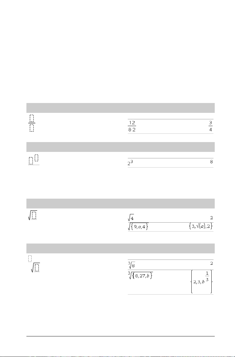
Fraction template
Note: See also / (divide), page 129.
e to move the cursor to each element’s position, and type a
· or /· to evaluate the expression.
/p keys
Example:
Exponent template
Note: Type the first value, press l, and then type the
exponent. To return the cursor to the baseline, press right arrow (¢).
Note: See also ^ (power), page 130.
Square root template
Note: See also
Nth root template
Note: See also root(), page 91.
‡
() (square root), page 136.
l key
Example:
/q keys
Example:
/l keys
Example:
TI-Nspire™ CAS Reference Guide 1
Page 8
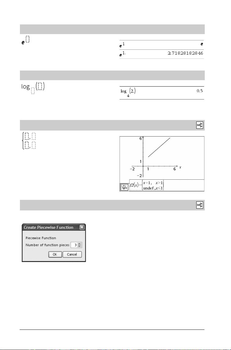
e exponent template
Natural exponential e raised to a power
Note: See also e^(), page 36.
u keys
Example:
Log template
Calculates log to a specified base. For a default of base 10, omit the
base.
Note: See also log(), page 62.
Piecewise template (2-piece)
Lets you create expressions and conditions for a two-piece piecewise
function. To add a piece, click in the template and repeat the
template.
Note: See also piecewise(), page 78.
Piecewise template (N-piece)
Lets you create expressions and conditions for an N-piece piecewise
function. Prompts for N.
/s key
Example:
Catalog >
Example:
Catalog >
Example:
See the example for Piecewise template (2-piece).
Note: See also piecewise(), page 78.
2 TI-Nspire™ CAS Reference Guide
Page 9
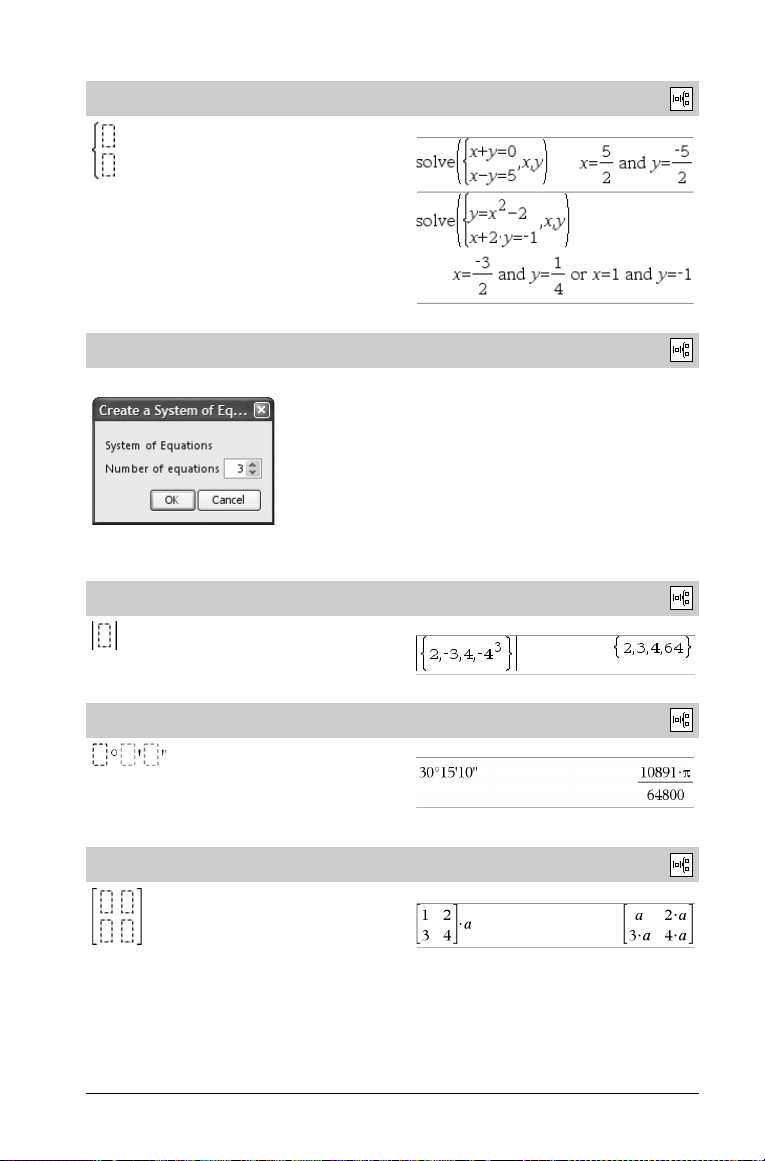
System of 2 equations template
Creates a system of two equations. To add a row to an existing
system, click in the template and repeat the template.
Note: See also system(), page 108.
Catalog >
Example:
System of N equations template
Lets you create a system of N equations. Prompts for N.
Note: See also system(), page 108.
Absolute value template
Note: See also abs(), page 6.
dd°mm’ss.ss’’ template
Lets you enter angles in dd°mm’ss.ss’’ format, where dd is the
number of decimal degrees, mm is the number of minutes, and ss.ss
is the number of seconds.
Matrix template (2 x 2)
Catalog >
Example:
See the example for System of equations template (2-equation).
Catalog >
Example:
Catalog >
Example:
Catalog >
Example:
Creates a 2 x 2 matrix.
TI-Nspire™ CAS Reference Guide 3
Page 10
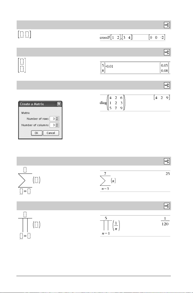
Matrix template (1 x 2)
.
Catalog >
Example:
Matrix template (2 x 1)
Matrix template (m x n)
The template appears after you are prompted to specify the number
of rows and columns.
Note: If you create a matrix with a large number of rows and
columns, it may take a few moments to appear.
Sum template (G)
Catalog >
Example:
Catalog >
Example:
Catalog >
Example:
Product template (Π)
Example:
Note: See also Π() (product), page 136.
Catalog >
4 TI-Nspire™ CAS Reference Guide
Page 11
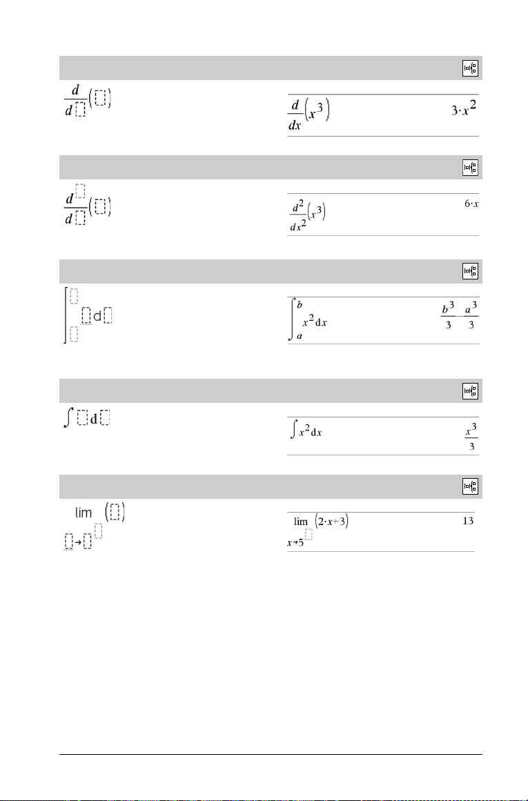
First derivative template
Catalog >
Example:
Note: See also
d() (derivative)
, page 135.
Nth derivative template
Note: See also
d() (derivative)
, page 135.
Definite integral template
Note: See also ‰() integrate(), page 135.
indefinite integral template
Note: See also
‰()
integrate()
, page 135.
Limit template
Catalog >
Example:
Catalog >
Example:
Catalog >
Example:
Catalog >
Example:
Use N or (N) for left hand limit. Use + for right hand limit.
Note: See also limit(), page 55.
TI-Nspire™ CAS Reference Guide 5
Page 12
Alphabetical listing
Items whose names are not alphabetic (such as +, !, and >) are listed at the end of this section,
starting on page 128. Unless otherwise specified, all examples in this section were performed
in the default reset mode, and all variables are assumed to be undefined.
A
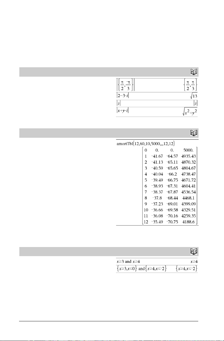
abs()
abs(Expr1) ⇒ expression
abs(
List1) ⇒ list
abs(Matrix1) ⇒ matrix
Returns the absolute value of the argument.
Note: See also Absolute value template, page 3.
If the argument is a complex number, returns the number’s modulus.
Note: All undefined variables are treated as real variables.
amortTbl()
amortTbl(NPmt,N,I,PV, [Pmt], [FV], [PpY], [CpY], [PmtAt],
roundValue]) ⇒ matrix
[
Amortization function that returns a matrix as an amortization table
for a set of TVM arguments.
NPmt is the number of payments to be included in the table. The
table starts with the first payment.
N, I, PV, Pmt, FV, PpY, CpY, and PmtAt are described in the table
of TVM arguments, page 117.
• If you omit Pmt, it defaults to
Pmt=tvmPmt(N,I,PV,FV,PpY,CpY,PmtAt).
• If you omit FV, it defaults to FV=0.
• The defaults for PpY, CpY, and PmtAt are the same as for the
TVM functions.
roundValue specifies the number of decimal places for rounding.
Default=2.
The columns in the result matrix are in this order: Payment number,
amount paid to interest, amount paid to principal, and balance.
The balance displayed in row n is the balance after payment n.
You can use the output matrix as input for the other amortization
functions GInt() and GPrn(), page 138, and bal(), page 11.
Catalog
Catalog
>
>
and
BooleanExpr1 and BooleanExpr2 ⇒ Boolean expression
BooleanList1 and BooleanList2 ⇒ Boolean list
BooleanMatrix1 and BooleanMatrix2 ⇒ Boolean matrix
Returns true or false or a simplified form of the original entry.
Catalog
>
6 TI-Nspire™ CAS Reference Guide
Page 13
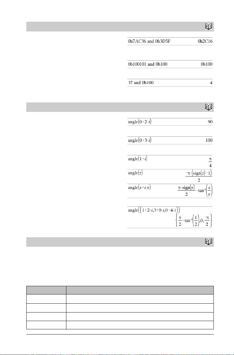
and
Integer1 and Integer2 ⇒ integer
Compares two real integers bit-by-bit using an
Internally, both integers are converted to signed, 64-bit binary
numbers. When corresponding bits are compared, the result is 1 if
both bits are 1; otherwise, the result is 0. The returned value
represents the bit results, and is displayed according to the Base
mode.
You can enter the integers in any number base. For a binary or
hexadecimal entry, you must use the 0b or 0h prefix, respectively.
Without a prefix, integers are treated as decimal (base 10).
If you enter a decimal integer that is too large for a signed, 64-bit
binary form, a symmetric modulo operation is used to bring the value
into the appropriate range.
and operation.
Catalog
>
In Hex base mode:
Important: Zero, not the letter O.
In Bin base mode:
In Dec base mode:
Note: A binary entry can have up to 64 digits (not counting the
0b prefix). A hexadecimal entry can have up to 16 digits.
angle()
angle(Expr1) ⇒ expression
Returns the angle of the argument, interpreting the argument as a
complex number.
Note: All undefined variables are treated as real variables.
angle(List1) ⇒ list
angle(Matrix1) ⇒ matrix
Returns a list or matrix of angles of the elements in List1 or Matrix1,
interpreting each element as a complex number that represents a
two-dimensional rectangular coordinate point.
ANOVA
ANOVA List1,List2[,List3,...,List20][,Flag]
Performs a one-way analysis of variance for comparing the means of
two to 20 populations. A summary of results is stored in the
stat.results variable. (See page 105.)
Flag=0 for Data, Flag=1 for Stats
In Degree angle mode:
In Gradian angle mode:
In Radian angle mode:
Catalog
Catalog
>
>
Output variable Description
stat.F Value of the F statistic
stat.PVal Smallest level of significance at which the null hypothesis can be rejected
stat.df Degrees of freedom of the groups
stat.SS Sum of squares of the groups
TI-Nspire™ CAS Reference Guide 7
Page 14

Output variable Description
stat.MS Mean squares for the groups
stat.dfError Degrees of freedom of the errors
stat.SSError Sum of squares of the errors
stat.MSError Mean square for the errors
stat.sp Pooled standard deviation
stat.xbarlist Mean of the input of the lists
stat.CLowerList 95% confidence intervals for the mean of each input list
stat.CUpperList 95% confidence intervals for the mean of each input list
ANOVA2way
ANOVA2way List1,List2[,List3,…,List20][,levRow]
Computes a two-way analysis of variance for comparing the means of
two to 20 populations. A summary of results is stored in the
stat.results variable. (See page 105.)
LevRow=0 for Block
LevRow=2,3,...,Len-1, for Two Factor, where
Len=length(List1)=length(List2) = … = length(List10) and
Len / LevRow ∈ {2,3,…}
Outputs: Block Design
Output variable Description
stat.FF statistic of the column factor
stat.PVal Smallest level of significance at which the null hypothesis can be rejected
stat.df Degrees of freedom of the column factor
stat.SS Sum of squares of the column factor
stat.MS Mean squares for column factor
stat.FBlock F statistic for factor
stat.PValBlock Least probability at which the null hypothesis can be rejected
stat.dfBlock Degrees of freedom for factor
stat.SSBlock Sum of squares for factor
stat.MSBlock Mean squares for factor
stat.dfError Degrees of freedom of the errors
stat.SSError Sum of squares of the errors
stat.MSError Mean squares for the errors
stat.s Standard deviation of the error
Catalog
>
8 TI-Nspire™ CAS Reference Guide
Page 15

COLUMN FACTOR Outputs
Output variable Description
stat.Fcol F statistic of the column factor
stat.PValCol Probability value of the column factor
stat.dfCol Degrees of freedom of the column factor
stat.SSCol Sum of squares of the column factor
stat.MSCol Mean squares for column factor
ROW FACTOR Outputs
Output variable Description
stat.FRow F statistic of the row factor
stat.PValRow Probability value of the row factor
stat.dfRow Degrees of freedom of the row factor
stat.SSRow Sum of squares of the row factor
stat.MSRow Mean squares for row factor
INTERACTION Outputs
Output variable Description
stat.FInteract F statistic of the interaction
stat.PValInteract Probability value of the interaction
stat.dfInteract Degrees of freedom of the interaction
stat.SSInteract Sum of squares of the interaction
stat.MSInteract Mean squares for interaction
ERROR Outputs
Output variable Description
stat.dfError Degrees of freedom of the errors
stat.SSError Sum of squares of the errors
stat.MSError Mean squares for the errors
s Standard deviation of the error
TI-Nspire™ CAS Reference Guide 9
Page 16
Ans
Ans ⇒ value
Returns the result of the most recently evaluated expression.
/v
keys
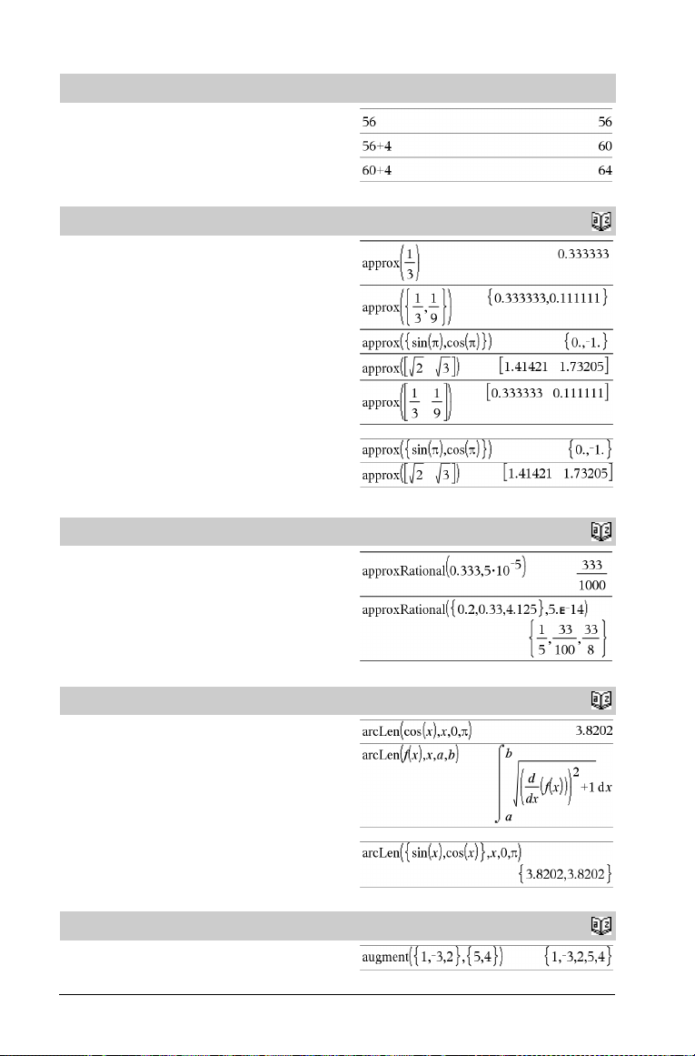
approx()
approx(Expr1) ⇒ expression
Returns the evaluation of the argument as an expression containing
decimal values, when possible, regardless of the current Auto or
Approximate
This is equivalent to entering the argument and pressing
mode.
/
·.
approx(List1) ⇒ list
approx(Matrix1) ⇒ matrix
Returns a list or matrix where each element has been evaluated to a
decimal value, when possible.
approxRational()
approxRational(Expr[, tol]) ⇒ expression
approxRational(List[, tol]) ⇒ list
approxRational(Matrix[, tol]) ⇒ matrix
Returns the argument as a fraction using a tolerance of tol. If tol is
omitted, a tolerance of 5.E-14 is used.
arcLen()
arcLen(Expr1,Var ,St art,End) ⇒ expression
Returns the arc length of Expr1 from Start to End with respect to
variable Var .
Arc length is calculated as an integral assuming a function mode
definition.
Catalog
Catalog
Catalog
>
>
>
arcLen(List1,Var ,Start,End) ⇒ list
Returns a list of the arc lengths of each element of List1 from Start to
End with respect to Va r .
augment()
augment(List1, List2) ⇒ list
Returns a new list that is List2 appended to the end of List1.
Catalog
>
10 TI-Nspire™ CAS Reference Guide
Page 17
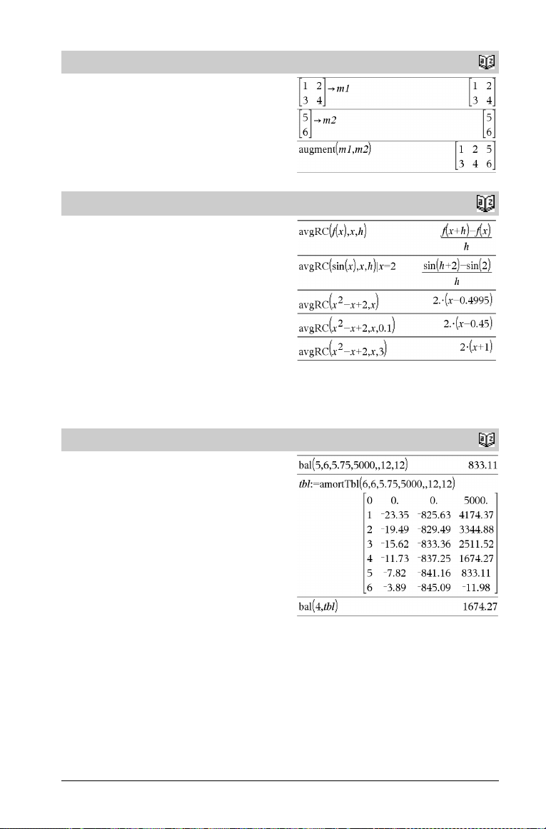
augment()
augment(Matrix1, Matrix2) ⇒ matrix
Returns a new matrix that is Matrix2 appended to Matrix1. When
the “,” character is used, the matrices must have equal row
dimensions, and Matrix2 is appended to Matrix1 as new columns.
Does not alter Matrix1 or Matrix2.
Catalog
>
avgRC()
avgRC(Expr1, Va r [=Value] [, H]) ⇒ expression
avgRC(Expr1, Va r [=Value] [, List1]) ⇒ list
avgRC(List1, Va r [=Value] [, H]) ⇒ list
avgRC(Matrix1, Var [=Value] [, H]) ⇒ matrix
Returns the forward-difference quotient (average rate of change).
Expr1 can be a user-defined function name (see Func).
When value is specified, it overrides any prior variable assignment o r
any current “such that” substitution for the variable.
H is the step value. If H is omitted, it defaults to 0.001.
Note that the similar function nDeriv() uses the central-difference
quotient.
B
bal()
bal(NPmt,N,I,PV ,[Pmt], [FV], [PpY], [CpY], [PmtAt],
roundValue]) ⇒ value
[
bal(NPmt,amortTable) ⇒ value
Amortization function that calculates schedule balance after a
specified payment.
N, I, PV, Pmt, FV, PpY, CpY, and PmtAt are described in the table
of TVM arguments, page 117.
NPmt specifies the payment number after which you want the data
calculated.
N, I, PV, Pmt, FV, PpY, CpY, and PmtAt are described in the table
of TVM arguments, page 117.
• If you omit Pmt, it defaults to
Pmt=tvmPmt(N,I,PV,FV,PpY,CpY,PmtAt).
• If you omit FV, it defaults to FV=0.
• The defaults for PpY, CpY, and PmtAt are the same as for the
TVM functions.
roundValue specifies the number of decimal places for rounding.
Default=2.
bal(NPmt,amortTable) calculates the balance after payment
number NPmt, based on amortization table amortTable. The
amortTable argument must be a matrix in the form described under
amortTbl(), page 6.
Note: See also GInt() and GPrn(), page 138.
Catalog
Catalog
>
>
TI-Nspire™ CAS Reference Guide 11
Page 18
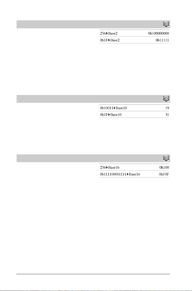
4Base2
4Base2 ⇒ integer
Integer1
Converts Integer1 to a binary number. Binary or hexadecimal
numbers always have a 0b or 0h prefix, respectively.
0b binaryNumber
0h hexadecimalNumber
Zero, not the letter O, followed by b or h.
A binary number can have up to 64 digits. A hexadecimal number can
have up to 16.
Without a prefix, Integer1 is treated as decimal (base 10). The result
is displayed in binary, regardless of the Base mode.
If you enter a decimal integer that is too large for a signed, 64-bit
binary form, a symmetric modulo operation is used to bring the value
into the appropriate range.
Catalog
>
4Base10
Integer1 4Base10 ⇒ integer
Converts Integer1 to a decimal (base 10) number. A binary or
hexadecimal entry must always have a 0b or 0h prefix, respectively.
0b binaryNumber
0h hexadecimalNumber
Zero, not the letter O, followed by b or h.
A binary number can have up to 64 digits. A hexadecimal number can
have up to 16.
Without a prefix, Integer1 is treated as decimal. The result is
displayed in decimal, regardless of the Base mode.
4Base16
Integer1 4Base16 ⇒ integer
Converts Integer1 to a hexadecimal number. Binary or hexadecimal
numbers always have a 0b or 0h prefix, respectively.
0b binaryNumber
0h hexadecimalNumber
Zero, not the letter O, followed by b or h.
A binary number can have up to 64 digits. A hexadecimal number can
have up to 16.
Without a prefix, Integer1 is treated as decimal (base 10). The result
is displayed in hexadecimal, regardless of the Base mode.
If you enter a decimal integer that is too large for a signed, 64-bit
binary form, a symmetric modulo operation is used to bring the value
into the appropriate range.
Catalog
Catalog
>
>
12 TI-Nspire™ CAS Reference Guide
Page 19
binomCdf()
binomCdf(n,p,lowBound,upBound) ⇒ number if lowBound
upBound are numbers, list if lowBound and upBound are
and
lists
binomCdf(
list if upBound is a list
Computes a cumulative probability for the discrete binomial
distribution with n number of trials and probability p of success on
each trial.
For P(X upBound), set lowBound=0
n,p,upBound) ⇒ number if upBound is a number,
Catalog
>
binomPdf()
binomPdf(n,p) ⇒ number
binomPdf(n,p,XVal) ⇒ number if XVal is a number, list if
XVal is a list
Computes a probability for the discrete binomial distribution with n
number of trials and probability p of success on each trial.
C
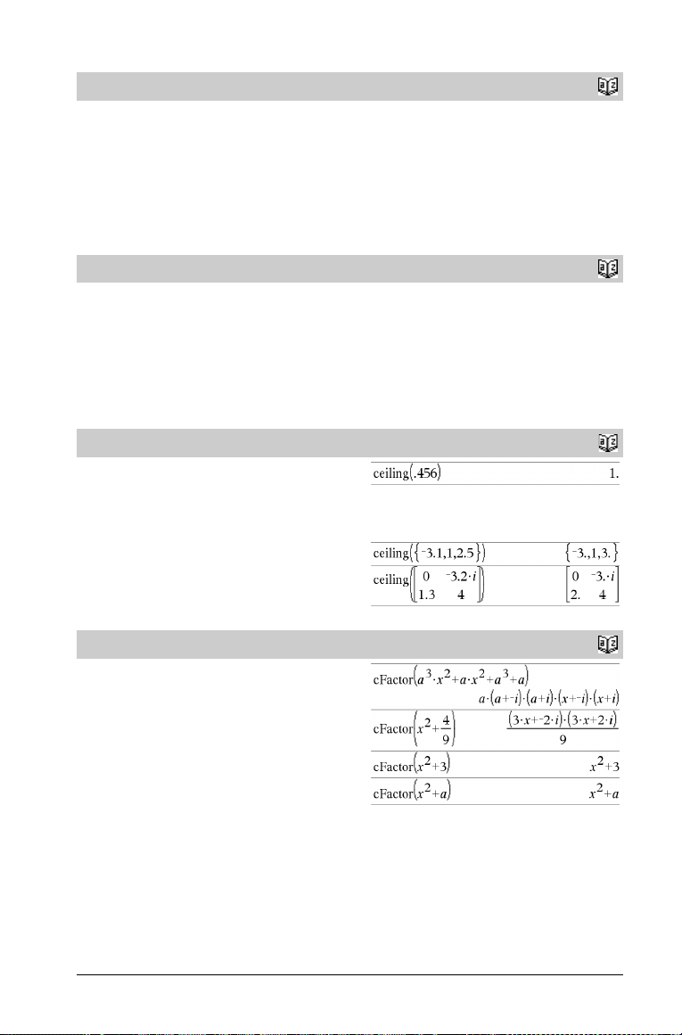
ceiling()
ceiling(Expr1) ⇒ integer
Returns the nearest integer that is ‚ the argument.
The argument can be a real or a complex number.
Note: See also floor().
ceiling(List1) ⇒ list
ceiling(Matrix1) ⇒ matrix
Returns a list or matrix of the ceiling of each element.
cFactor()
cFactor(Expr1[,Var ]) ⇒ expression
cFactor(List1[,Va r]) ⇒ list
cFactor(Matrix1[,Var ]) ⇒ matrix
cFactor(Expr1) returns Expr1 factored with respect to all of its
variables over a common denominator.
Expr1 is factored as much as possible toward linear rational factors
even if this introduces new non-real numbers. This alternative is
appropriate if you want factorization with respect to more than one
variable.
Catalog
Catalog
Catalog
>
>
>
TI-Nspire™ CAS Reference Guide 13
Page 20
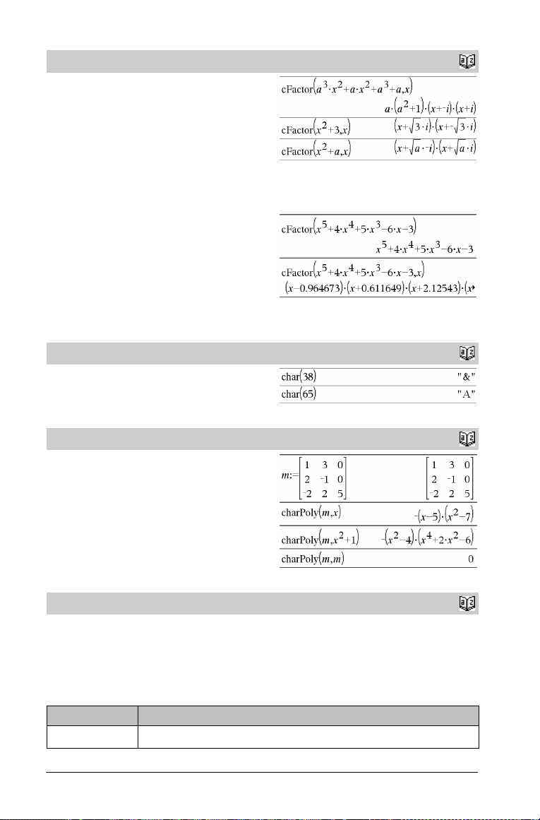
cFactor()
cFactor(Expr1,Var ) returns Expr1 factored with respect to variable
Var .
Expr1 is factored as much as possible toward factors that are linear
in Va r, with perhaps non-real constants, even if it introduces
irrational constants or subexpressions that are irrational in other
variables.
The factors and their terms are sorted with Va r as the main variable.
Similar powers of Va r are collected in each factor. Include Va r if
factorization is needed with respect to only that variable and you are
willing to accept irrational expressions in any other variables to
increase factorization with respect to Va r . There might be some
incidental factoring with respect to other variables.
For the Auto setting of the Auto or Approximate mode,
including Va r also permits approximation with floating-point
coefficients where irrational coefficients cannot be explicitly
expressed concisely in terms of the built-in functions. Even when
there is only one variable, including Va r might yield more complete
factorization.
Note: See also factor().
Catalog
>
To see the entire result, press £ and then use ¡ and ¢ to
move the cursor.
char()
char(Integer) ⇒ character
Returns a character string containing the character numbered Integer
from the handheld character set. The valid range for Integer is 0–
65535.
charPoly()
charPoly(squareMatrix,Var) ⇒ polynomial expression
charPoly(squareMatrix,Expr) ⇒ polynomial expression
charPoly(squareMatrix1,Matrix2) ⇒ polynomial expression
Returns the characteristic polynomial of squareMatrix. The
characteristic polynomial of n×n matrix A, denoted by pA(l), is the
polynomial defined by
pA(l) = det(l• I NA)
where I denotes the n×n identity matrix.
squareMatrix1 and squareMatrix2 must have the equal dimensions.
2
c
2way
2
c
2way obsMatrix
chi22way obsMatrix
Computes a c2 test for association on the two-way table of counts in
the observed matrix obsMatrix. A summary of results is stored in the
stat.results variable. (See page 105.)
Output variable Description
stat.c2 Chi square stat: sum (observed - expected)2/expected
Catalog
Catalog
Catalog
>
>
>
14 TI-Nspire™ CAS Reference Guide
Page 21

Output variable Description
stat.PVal Smallest level of significance at which the null hypothesis can be rejected
stat.df Degrees of freedom for the chi square statistics
stat.ExpMat Matrix of expected elemental count table, assuming null hypothesis
stat.CompMat Matrix of elemental chi square statistic contributions
2
c
Cdf()
2
c
Cdf(lowBound,upBound,df) ⇒ number if lowBound and
upBound are numbers, list if lowBound and upBound are lists
chi2Cdf(
lowBound,upBound,df) ⇒ number if lowBound and
upBound are numbers, list if lowBound and upBound are lists
Computes the c2 distribution probability between lowBound and
upBound for the specified degrees of freedom df.
For P(X upBound), set lowBound = 0.
2
c
GOF
2
c
GOF obsList,expList,df
chi2GOF obsList,expList,df
Performs a test to confirm that sample data is from a population that
conforms to a specified distribution. obsList is a list of counts and
must contain integers. A summary of results is stored in the
stat.results variable. (See page 105.)
Output variable Description
stat.c2 Chi square stat: sum((observed - expected)2/expected
stat.PVal Smallest level of significance at which the null hypothesis can be rejected
stat.df Degrees of freedom for the chi square statistics
stat.CompList Elemental chi square statistic contributions
Catalog
Catalog
>
>
2
c
Pdf()
2
c
Pdf(XVal,df) ⇒ number if XVal is a number, list if XVal is a
list
chi2Pdf(
XVal,df) ⇒ number if XVal is a number, list if XVal is
a list
Computes the probability density function (pdf) for the c2 distribution
at a specified XVal value for the specified degrees of freedom df.
Catalog
>
TI-Nspire™ CAS Reference Guide 15
Page 22
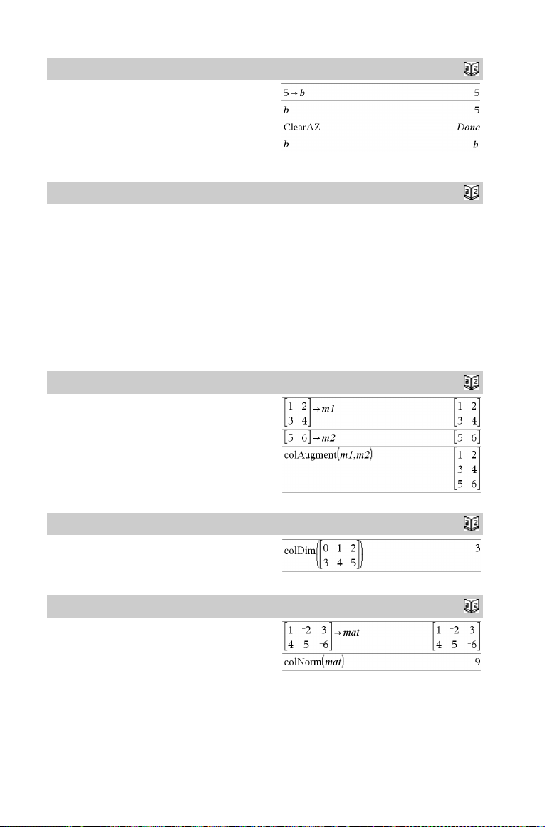
ClearAZ
ClearAZ
Clears all single-character variables in the current problem space.
Catalog
>
ClrErr
ClrErr
Clears the error status and sets system variable errCode to zero.
The Else claus e of the Try...Else...EndTry block should use ClrErr
or PassErr. If the error is to be processed or ignored, use ClrErr. If
what to do with the error is not known, us e PassErr to se nd it to the
next error handler. If there are no more pendin g Try...Else...EndTry
error handlers, the error dialog box will be displayed as normal.
Note: See also PassErr, page 78, and Try , page 115.
Note for entering the example: In the Calculator application
on the handheld, you can enter multi-line definitions by pressing
@ instead of · at the end of each line. On the computer
keyboard, hold down Alt and press Enter.
colAugment()
colAugment(Matrix1, Matrix2) ⇒ matrix
Returns a new matrix that is Matrix2 appended to Matrix1. The
matrices must have equal column dimensions, and Matrix2 is
appended to Matrix1 as new rows. Does not alter Matrix1 or
Matrix2.
colDim()
colDim(Matrix) ⇒ expression
Returns the number of columns contained in Matrix.
Note: See also rowDim() .
Catalog
For an example of ClrErr, See Example 2 under the Try
command, page 115.
Catalog
Catalog
>
>
>
colNorm()
colNorm(Matrix) ⇒ expression
Returns the maximum of the sums of the absolute values of the
elements in the columns in Matrix.
Note: Undefined matrix elements are not allowed. See also
rowNorm().
Catalog
>
16 TI-Nspire™ CAS Reference Guide
Page 23
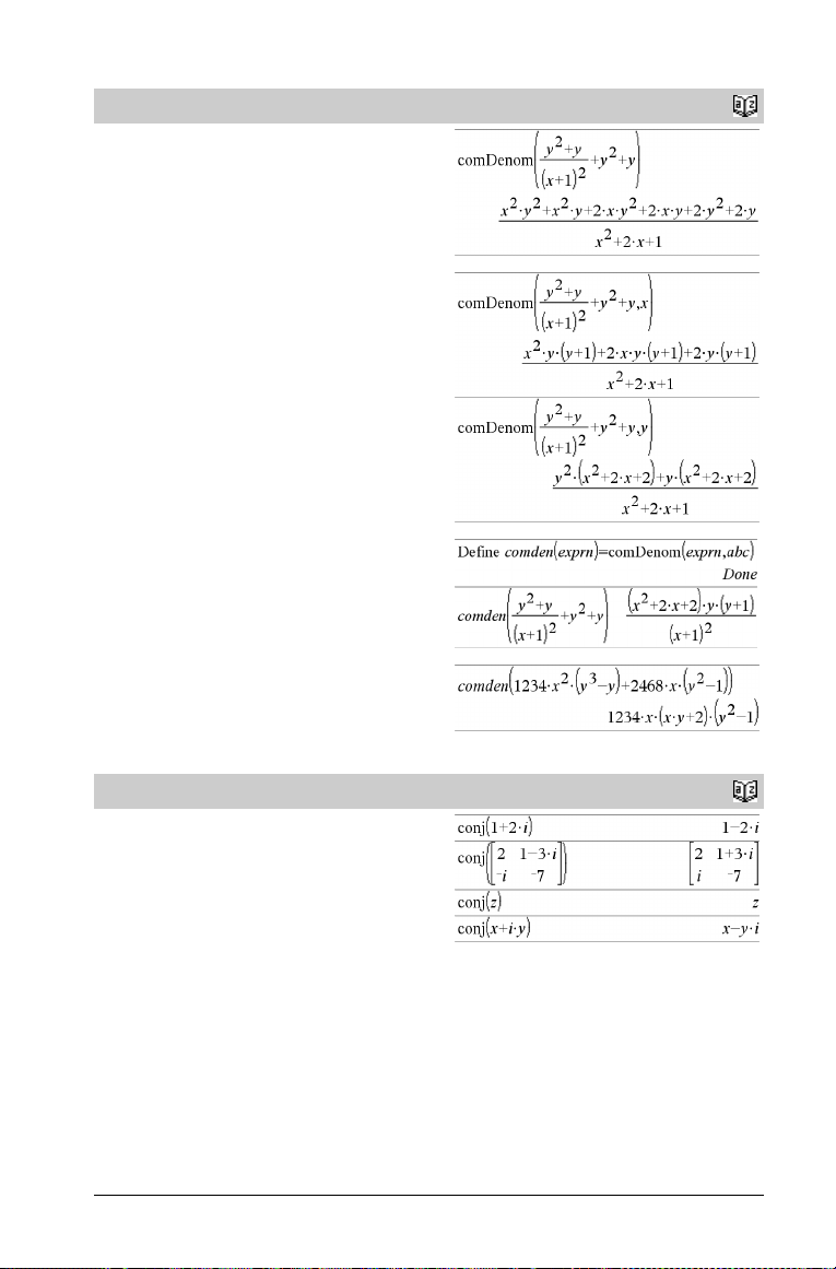
comDenom()
comDenom(Expr1[,Va r]) ⇒ expression
comDenom(List1[,Var ]) ⇒ list
comDenom(Matrix1[,Var ]) ⇒ matrix
comDenom(Expr1) returns a reduced ratio of a fully expanded
numerator over a fully expanded denominator.
comDenom(Expr1,Va r) returns a reduced ratio of numerator and
denominator expanded with respect to Va r . The terms and their
factors are sorted with Var as the main variable. Similar powers of
Var are collected. There might be some incidental factoring of the
collected coefficients. Compared to omitting Va r , this often saves
time, memory, and screen space, while making the expression more
comprehensible. It also makes subsequent operations on the result
faster and less likely to exhaust memory.
If Var does not occur in Expr1, comDenom(Expr1,Var ) returns a
reduced ratio of an unexpanded numerator over an unexpanded
denominator. Such results usually save even more time, memor y, and
screen space. Such partially factored results also make subsequent
operations on the result much faster and much less likely to exhaust
memory.
Even when there is no denominator, the comden function is often a
fast way to achieve partial factorization if factor() is too slow or if it
exhausts memory.
Hint: Enter this comden() function definition and routinely try it as
an alternative to comDenom() and factor().
Catalog
>
conj()
conj(Expr1) ⇒ expression
conj(List1) ⇒ list
conj(Matrix1) ⇒ matrix
Catalog
>
Returns the complex conjugate of the argument.
Note: All undefined variables are treated as real variables.
TI-Nspire™ CAS Reference Guide 17
Page 24
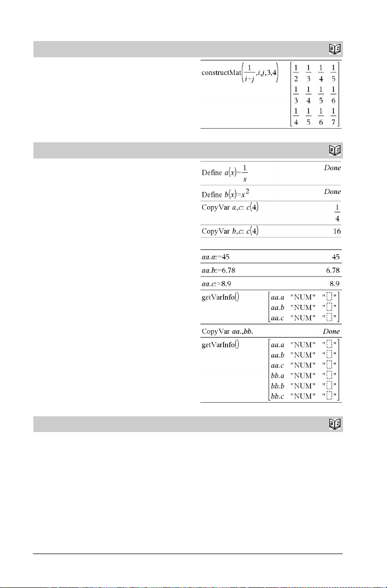
constructMat()
constructMat(Expr,Var 1 ,Var 2 ,numRows,numCols)
⇒ matrix
Returns a matrix based on the arguments.
Expr is an expression in variables Va r 1 and Va r 2 . Elements in the
resulting matrix are formed by evaluating Expr for each incremented
value of Var 1 and Va r 2.
Var 1 is automatically incremented from
each row, Va r2 is incremented from 1 through numCols.
1 through numRows. Within
Catalog
>
CopyVar
CopyVar Var 1 , Va r 2
CopyVar Var 1 ., Va r2 .
CopyVar Var 1 , Var 2 copies the value of variable Va r 1 to variable
Var 2 , creating Va r 2 if necessary. Variable Va r1 must have a value.
If Var 1 is the name of an existing user-defined function, copies the
definition of that function to function Va r 2. Function Va r 1 must be
defined.
Var 1 must meet the variable-naming requirements or must be an
indirection expression that simplifies to a variable name meeting the
requirements.
CopyVar Var 1 ., Va r 2. copies all members of the Var 1 . variable
group to the Var 2 . group, creating Var 2 . if necessary.
Var 1 . must be the name of an existing variable group, such as the
statistics stat.nn results, or variables created using the
LibShortcut() function. If Var 2 . already exists, this command
replaces all members that are common to both groups and adds the
members that do not already exist. If a simple (non-group) variable
named Va r2 exists, an error occurs.
corrMat()
corrMat(List1,List2[,…[,List20]])
Computes the correlation matrix for the augmented matrix [List1,
List2, ..., List20].
Catalog
Catalog
>
>
18 TI-Nspire™ CAS Reference Guide
Page 25
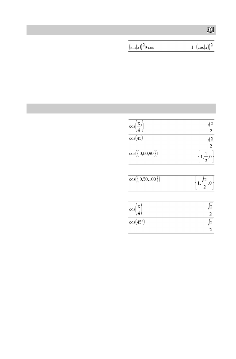
4
cos
4cos
Expr
Represents Expr in terms of cosine. This is a display conversion
operator. It can be used only at the end of the entry line.
4
cos reduces all powers of
sin(...) modulo 1Ncos(...)^2
so that any remaining powers of cos(...) have exponents in the range
(0, 2). Thus, the result will be free of sin(...) if and only if sin(...)
occurs in the given expression only to even powers.
Note: This conversion operator is not supported in Degree or
Gradian Angle modes. Before using it, make sure that the Angle
mode is set to Radians and that Expr does not contain explicit
references to degree or gradian angles.
Catalog
>
cos()
cos(Expr1) ⇒ expression
cos(List1) ⇒ list
cos(Expr1) returns the cosine of the argument as an expression.
cos(List1) returns a list of the cosines of all elements in List1.
Note: The argument is interpreted as a degree, gradian or radian
angle, according to the current angle mode settin g. You can use ó,G,
or ôto override the angle mode temporarily.
n key
In Degree angle mode:
In Gradian angle mode:
In Radian angle mode:
TI-Nspire™ CAS Reference Guide 19
Page 26
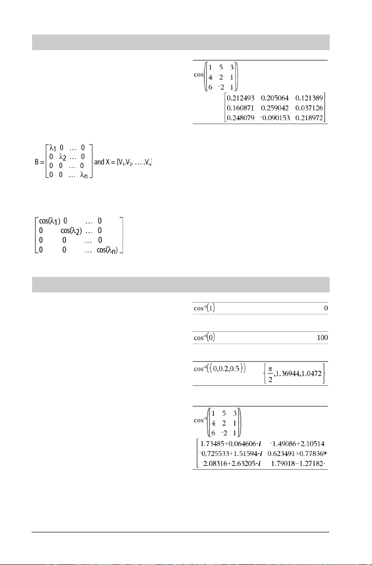
cos()
cos(squareMatrix1) ⇒ squareMatrix
Returns the matrix cosine of squareMatrix1. This is not the same as
calculating the cosine of each element.
When a scalar function f(A) operates on squareMatrix1 (A), the
result is calculated by the algorithm:
Compute the eigenvalues (li) and eigenvectors (Vi) of A.
squareMatrix1 must be diagonalizable. Also, it cannot have symbolic
variables that have not been assigned a value.
Form the matrices:
Then A = X B Xêand f(A) = X f(B) Xê. For example, cos(A) = X cos(B)
Xê where:
cos(B) =
All computations are performed using floating-point arithmetic.
n key
In Radian angle mode:
cosê()
cosê(Expr1) ⇒ expression
cosê(List1) ⇒ list
cosê(Expr1) returns the angle whose cosine is Expr1 as an
expression.
cosê(List1) returns a list of the inverse cosines of each element of
List1.
Note: The result is returned as a degree, gradian or radian angle,
according to the current angle mode setting.
cosê(squareMatrix1) ⇒ squareMatrix
Returns the matrix inverse cosine of squareMatrix1. This is not the
same as calculating the inverse cosine of each element. For
information about the calculation method, refer to cos().
squareMatrix1 must be diagonalizable. The result always contains
floating-point numbers.
In Degree angle mode:
In Gradian angle mode:
In Radian angle mode:
In Radian angle mode and Rectangular Complex Format:
To see the entire result, press £ and then use ¡ and ¢ to
move the cursor.
/n keys
20 TI-Nspire™ CAS Reference Guide
Page 27
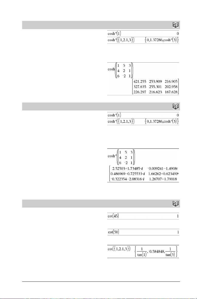
cosh()
cosh(Expr1) ⇒ expression
cosh(List1) ⇒ list
cosh(Expr1) returns the hyperbolic cosine of the argument as an
expression.
cosh(List1) returns a list of the hyperbolic cosines of each element o f
List1.
cosh(squareMatrix1) ⇒ squareMatrix
Returns the matrix hyperbolic cosine of squareMatrix1. This is not
the same as calculating the hyperbolic cosine of each element. For
information about the calculation method, refer to
squareMatrix1 must be diagonalizable. The result always contains
floating-point numbers.
cos().
In Radian angle mode:
Catalog
>
coshê()
coshê(Expr1) ⇒ expression
coshê(List1) ⇒ list
ê
cosh
(Expr1) returns the inverse hyperbolic cosine of the argument
as an expression.
ê
cosh
(List1) returns a list of the inverse hyperbolic cosines of each
element of List1.
coshê(squareMatrix1) ⇒ squareMatrix
Returns the matrix inverse hyperbolic cosine of squareMatrix1. This
is not the same as calculating the inverse hyperbolic cosine of each
element. For information about the calculation method, refer to
cos().
squareMatrix1 must be diagonalizable. The result always contains
floating-point numbers.
cot()
cot(Expr1) ⇒ expression
cot(List1) ⇒ list
Returns the cotangent of Expr1 or returns a list of the cotangents of
all elements in List1.
Note: The argument is interpreted as a degree, gradian or radian
angle, according to the current angle mode settin g. You can use ó,G,
orôto override the angle mode temporarily.
Catalog
>
In Radian angle mode and In Rectangular Complex Format:
To see the entire result, press £ and then use ¡ and ¢ to
move the cursor.
Catalog
>
In Degree angle mode:
In Gradian angle mode:
In Radian angle mode:
TI-Nspire™ CAS Reference Guide 21
Page 28
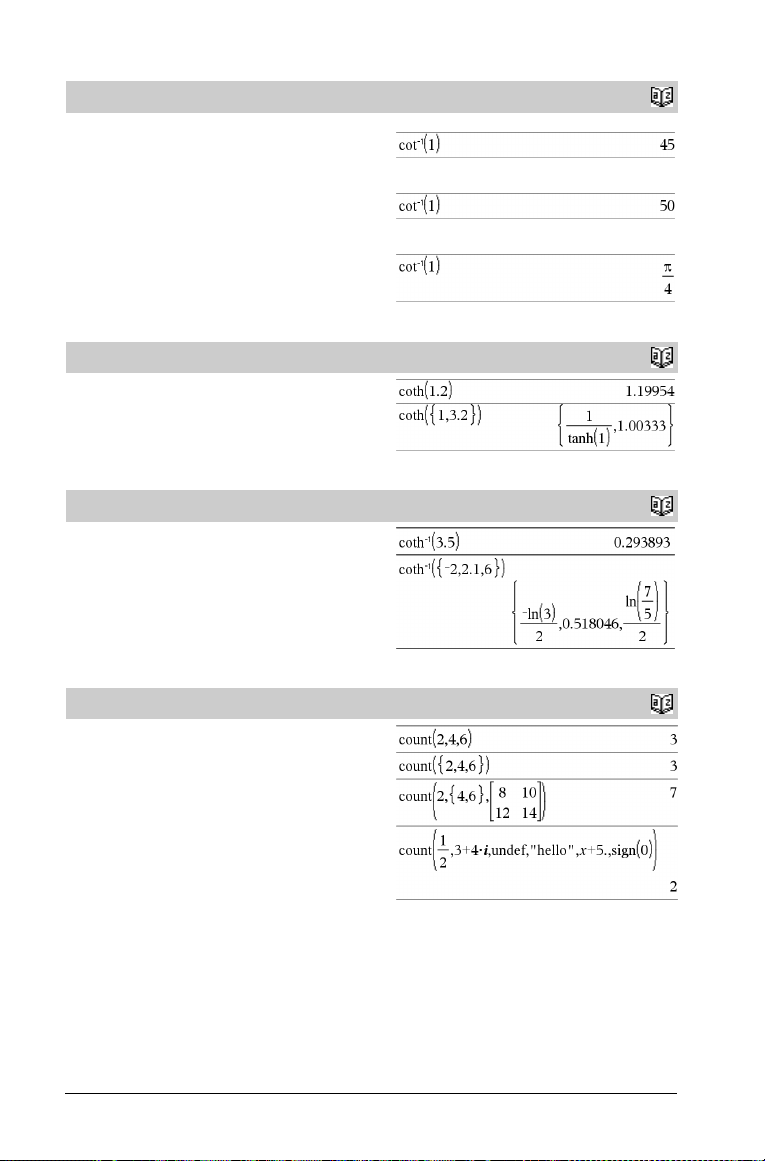
cotê()
cotê(Expr1) ⇒ expression
cotê(List1) ⇒ list
Returns the angle whose cotangent is Expr1 or returns a list
containing the inverse cotangents of each element of List1.
Note: The result is returned as a degree, gradian or radian angle,
according to the current angle mode setting.
In Degree angle mode:
In Gradian angle mode:
In Radian angle mode:
Catalog
>
coth()
coth(Expr1) ⇒ expression
coth(List1) ⇒ list
Returns the hyperbolic cotangent of Expr1 or returns a list of the
hyperbolic cotangents of all elements of List1.
cothê()
cothê(Expr1) ⇒ expression
cothê(List1) ⇒ list
Returns the inverse hyperbolic cotangent of Expr1 or returns a list
containing the inverse hyperbolic cotangents of each element of
List1.
count()
count(Val u e 1 or L i s t1 [,Value2orList2 [,...]]) ⇒ value
Returns the accumulated count of all elements in the arguments that
evaluate to numeric values.
Each argument can be an expression, value, list, or matrix. You can
mix data types and use arguments of various dimensions.
For a list, matrix, or range of cells, each element is evaluated to
determine if it should be included in the count.
Within the Lists & Spreadsheet application, you can use a range of
cells in place of any argument.
Catalog
>
Catalog
>
Catalog
>
In the last example, only 1/2 and 3+4*i are counted. The
remaining arguments, assuming x is undefined, do not evaluate
to numeric values.
22 TI-Nspire™ CAS Reference Guide
Page 29
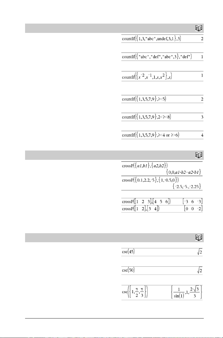
countif()
countif(List,Criteria) ⇒ value
Returns the accumulated count of all elements in List that meet the
specified Criteria.
Criteria can be:
• A value, expression, or string. For example, 3 counts only those
elements in List that simplify to the value 3.
• A Boolean expression containing the symbol ? as a placeholder
for each element. For example, ?<5 counts only those elements
in List that are less than 5.
Within the Lists & Spreadsheet application, you can use a range of
cells in place of List.
Note: See also sumIf(), page 108, and frequency(), page 45.
Catalog
Counts the number of elements equal to 3.
Counts the number of elements equal to “def.”
Counts the number of elements equal to x; this example
assumes the variable x is undefined.
Counts 1 and 3.
Counts 3, 5, and 7.
Counts 1, 3, 7, and 9.
>
crossP()
crossP(List1, List2) ⇒ list
Returns the cross product of List1 and List2 as a list.
List1 and List2 must have equal dimension, and the dimension must
be either 2 or 3.
crossP(Vector1, Vector2) ⇒ vector
Returns a row or column vector (depending on the arguments) that is
the cross product of Vector1 and Vector2.
Both Vector1 and Vector2 must be row vectors, or both must be
column vectors. Both vectors must have equal dimension, and the
dimension must be either 2 or 3.
csc()
csc(Expr1) ⇒ expression
csc(List1) ⇒ list
Returns the cosecant of Expr1 or returns a list containing the
cosecants of all elements in List1.
In Degree angle mode:
In Gradian angle mode:
In Radian angle mode:
Catalog
Catalog
>
>
TI-Nspire™ CAS Reference Guide 23
Page 30
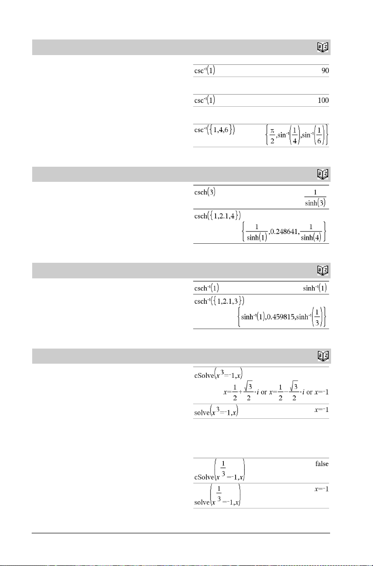
cscê()
cscê(Expr1) ⇒ expression
cscê(List1) ⇒ list
Returns the angle whose cosecant is Expr1 or returns a list
containing the inverse cosecants of each element of List1.
Note: The result is returned as a degree, gradian or radian angle,
according to the current angle mode setting.
In Degree angle mode:
In Gradian angle mode:
In Radian angle mode:
Catalog
>
csch()
csch(Expr1) ⇒ expression
csch(List1) ⇒ list
Returns the hyperbolic cosecant of Expr1 or returns a list of the
hyperbolic cosecants of all elements of List1.
cschê()
cschê(Expr1) ⇒ expression
cschê(List1) ⇒ list
Returns the inverse hyperbolic cosecant of Expr1 or returns a list
containing the inverse hyperbolic cosecants of each element of List1.
cSolve()
cSolve(Equation, Va r ) ⇒ Boolean expression
cSolve(Equation, Va r =G u e s s) ⇒ Boolean expression
cSolve(Inequality, Va r ) ⇒ Boolean expression
Returns candidate complex solutions of an equation or inequality for
Var . The goal is to produce candidates for all real and non-real
solutions. Even if Equation is real, cSolve() allows non-real results
in Real result Complex Format.
Although all undefined variables that do not end with an underscore
(_) are processed as if they were real, cSolve() can solve polynomial
equations for complex solutions.
cSolve() temporarily sets the domain to complex during the solution
even if the current domain is real. In the complex domain, fractional
powers having odd denominators use the principal rather than the
real branch. Consequently, solutions from solve() to equations
involving such fractional powers are not necessarily a subset of those
from cSolve().
Catalog
Catalog
Catalog
>
>
>
24 TI-Nspire™ CAS Reference Guide
Page 31

cSolve()
cSolve() starts with exact symbolic methods. cSolve() also uses
iterative approximate complex polynomial factoring, if necessary.
Note: See also cZeros(), solve(), and zeros().
Note: If Equation is non-polynomial with functions such as abs(),
angle(), conj(), real(), or imag(), you should place an
underscore (press
variable is treated as a real value.
If you use var_ , the variable is treated as complex.
You should also use var_ for any other variables in Equation that
might have unreal values. Otherwise, you may receive unexpected
results.
cSolve(Eqn1 and Eqn2 [and …],
VarOrGuess1, VarOrGuess2 [, … ]) ⇒ Boolean expression
cSolve(SystemOfEqns, VarOrGuess1,
VarOrGuess2 [, …]) ⇒ Boolean expression
Returns candidate complex solutions to the simultaneous algebraic
equations, where each varOrGuess specifies a variable that you
want to solve for.
Optionally, you can specify an initial guess for a variable. Each
varOrGuess must have the form:
variable
– or –
variable = real or non-real number
For example, x is valid and so is x=3+i.
If all of the equations are polynomials and if you do NOT specify any
initial guesses, cSolve() uses the lexical Gröbner/Buchberger
elimination method to attempt to determine all complex solutions.
Complex solutions can include both real and non-real solutions, as in
the example to the right.
/_) at the end of Var . By default, a
Catalog
>
In Display Digits mode of Fix 2:
To see the entire result, press
move the cursor.
z is treated as real:
z_ is treated as complex:
Note: The following examples use an underscore (press
£ and then use ¡ and ¢ to
/_) so that the variables will be treated as complex.
To see the entire result, press £ and then use ¡ and ¢ to
move the cursor.
Simultaneous polynomial equations can have extra variables that
have no values, but represent given numeric values that could be
substituted later.
To see the entire result, press £ and then use ¡ and ¢ to
move the cursor.
TI-Nspire™ CAS Reference Guide 25
Page 32

cSolve()
You can also include solution variables that do not appear in the
equations. These solutions show how families of solutions might
contain arbitrary constants of the form ck, w here k is an integer suffix
from 1 through 255.
For polynomial systems, computation time or memory exhaustion
may depend strongly on the order in which you list solution variables.
If your initial choice exhausts memory or your patience, try
rearranging the variables in the equations and/or varOrGuess list.
If you do not include any guesses and if any equation is nonpolynomial in any variable but all equations are linear in all solution
variables, cSolve() uses Gaussian elimination to attempt to
determine all solutions.
If a system is neither polynomial in all of its variables nor linear in its
solution variables, cSolve() determines at most one solution using
an approximate iterative method. To do so, the number of solution
variables must equal the number of equations, and all other vari ables
in the equations must simplify to numbers.
A non-real guess is often necessary to determine a non-real solution.
For convergence, a guess might have to be rather close to a solution.
Catalog
>
To see the entire result, press £ and then use ¡ and ¢ to
move the cursor.
To see the entire result, press £ and then use ¡ and ¢ to
move the cursor.
CubicReg
CubicReg X, Y[, [Freq] [, Category, Include]]
Computes the cubic polynomial regression y = a·x3+b·
x2+c·x+d on lists X and Y with frequency Freq. A summary of
results is stored in the stat.results variable. (See page 105.)
All the lists must have equal dimension except for Include.
X and Y are lists of independent and dependent variables.
Freq is an optional list of frequency values. Each element in Freq
specifies the frequency of occurrence for each corresponding X and Y
data point. The default value is 1. All elements must be integers | 0.
Category is a list of numeric category codes for the corresponding X
and Y data.
Include is a list of one or more of the category codes. Only those data
items whose category code is included in this list are included in the
calculation.
Output variable Description
stat.RegEqn
stat.a, stat.b, stat.c,
stat.d
2
stat.R
stat.Resid Residuals from the regression
stat.XReg List of data points in the modified X List actually used in the regression based on restrictions of Freq,
Regression equation: a·x3+b·x2+c·x+d
Regression coefficients
Coefficient of determination
Category List, and Include Categories
Catalog
>
26 TI-Nspire™ CAS Reference Guide
Page 33

Output variable Description
stat.YReg List of data points in the modified Y List actually used in the regression based on restrictions of Freq,
Category List, and Include Categories
stat.FreqReg List of frequencies corresponding to stat.XReg and stat.YReg
cumSum()
cumSum(List1) ⇒ list
Returns a list of the cumulative sums of the elements in List1,
starting at element 1.
cumSum(Matrix1) ⇒ matrix
Returns a matrix of the cumulative sums of the elements in Matrix1.
Each element is the cumulative sum of the column from top to
bottom.
Cycle
Cycle
Transfers control immediately to the next iteration of the cu rrent loop
(For, While, or Loop).
Cycle is not allowed outside the three looping structures (For,
While, or Loop).
Note for entering the example: In the Calculator
application on the handheld, you can enter multi-line definitions by
pressing @ instead of · at the end of each line. On the
computer keyboard, hold down Alt and press Enter.
Catalog
>
Catalog
>
Function listing that sums the integers from 1 to 100 skipping
50.
4Cylind
Catalog
>
Vec t o r 4Cylind
Displays the row or column vector in cylindrical form [r,q, z].
Vec t o r must have exactly three elements. It can be either a row or a
column.
cZeros()
cZeros(Expr, Va r ) ⇒ list
Returns a list of candidate real and non-real values of Va r that make
Expr=0. cZeros() does this by computing
exp4list(cSolve(Expr=0,Var ),Va r ). Otherwise, cZeros() is
similar to zeros().
Note: See also cSolve(), solve(), and zeros().
In Display Digits mode of Fix 3:
To see the entire result, press £ and then use ¡ and ¢ to
move the cursor.
Catalog
>
TI-Nspire™ CAS Reference Guide 27
Page 34
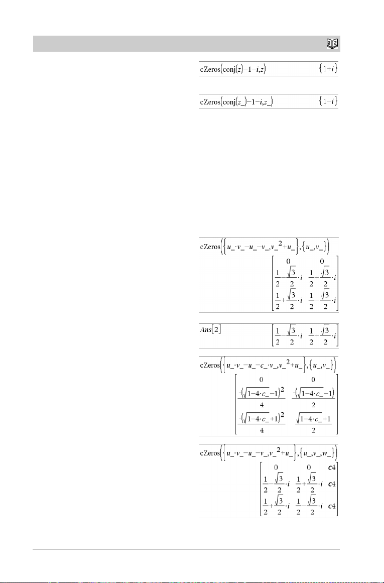
cZeros()
Note: If Expr is non-polynomial with functions such as abs(),
angle(), conj(), real(), or imag(), you should place an
underscore (press /_) at the end of Var . By default, a
variable is treated as a real value. If you use var_ , the variable is
treated as complex.
You should also use var_ for any other variables in Expr that might
have unreal values. Otherwise, you may receive unexpected results.
cZeros({Expr1, Expr2 [, … ] },
VarOrGuess1,VarOrGuess2 [, … ] }) ⇒ matrix
{
Returns candidate positions where the expressions are zero
simultaneously. Each VarOrGuess specifies an unknown whose
value you seek.
Optionally, you can specify an initial guess for a variable. Each
VarOrGuess must have the form:
variable
– or –
variable = real or non-real number
For example, x is valid and so is x=3+i.
If all of the expressions are polynomials and you do NOT specify any
initial guesses, cZeros() uses the lexical Gröbner/Buchberger
elimination method to attempt to determine all complex zeros.
Complex zeros can include both real and non-real zeros, as in the
example to the right.
Each row of the resulting matrix represents an alternate zero, with
the components ordered the same as the VarOrGuess list. To extract
a row, index the matrix by [row ].
Catalog
>
z is treated as real:
z_ is treated as complex:
Note: The following examples use an underscore _ (press
/_) so that the variables will be treated as complex.
Extract row 2:
Simultaneous polynomials can have extra variables that have no
values, but represent given numeric values that could be substituted
later.
You can also include unknown variables that do not appear in the
expressions. These zeros show how families of zeros might contain
arbitrary constants of the form ck, where k is an integer suffix from 1
through 255.
For polynomial systems, computation time or memory exhaustion
may depend strongly on the order in which you list unknowns. If your
initial choice exhausts memory or your patience, try rearranging the
variables in the expressions and/or VarOrGuess list.
28 TI-Nspire™ CAS Reference Guide
Page 35

cZeros()
If you do not include any guesses and if any expression is nonpolynomial in any variable but all expressions are linear in all
unknowns,
cZeros() uses Gaussian elimination to attempt to
determine all zeros.
If a system is neither polynomial in all of its variables nor linear in its
unknowns, cZeros() determines at most one zero using an
approximate iterative method. To do so, the number of unknowns
must equal the number of expressions, and all other variables in the
expressions must simplify to numbers.
A non-real guess is often necessary to determine a non-real zero. For
convergence, a guess might have to be rather close to a zero.
D
Catalog
>
dbd()
dbd(date1,date2) ⇒ value
Returns the number of days between date1 and date2 using the
actual-day-count method.
date1 and date2 can be numbers or lists of numbers within the range
of the dates on the standard calendar. If both date1 and date2 are
lists, they must be the same length.
date1 and date2 must be between the years 1950 through 2049.
You can enter the dates in either of two formats. The decimal
placement differentiates between the date formats.
MM.DDYY (format used commonly in the United States)
DDMM.YY (format use commonly in Europe)
4
DD
Expr1 4DD ⇒ value
List1 4DD ⇒ list
Matrix1 4DD ⇒ matrix
Returns the decimal equivalent of the argument expresse d in degrees.
The argument is a number, list, or matrix that is interpreted by the
Angle mode setting in gradians, radians or degrees.
In Degree angle mode:
In Gradian angle mode:
In Radian angle mode:
Catalog
Catalog
>
>
TI-Nspire™ CAS Reference Guide 29
Page 36

4Decimal
Expression1
List1
Matrix1
Displays the argument in decimal form. This operator can be used
only at the end of the entry line.
4Decimal
4Decimal
4
Decimal
⇒ expression
⇒ expression
⇒ expression
Catalog
>
Define
Define Var = Expression
Define Function(Param1, Param2, ...) = Expression
Defines the variable Var or the user-defined function Function.
Parameters, such as Param1, provide placeholders for passing
arguments to the function. When calling a user-defined function, you
must supply arguments (for example, values or variables) that
correspond to the parameters. When called, the function evaluates
Expression using the supplied arguments.
Var and Function cannot be the name of a system variable or built -in
function or command.
Note: This form of Define is equivalent to executing the
expression: expression & Function(Param1,Param2).
Define Function(Param1, Param2, ...) = Func
Block
EndFunc
Program(Param1, Param2, ...) = Prgm
Define
Block
EndPrgm
In this form, the user-defined function or program can execute a block
of multiple statements.
Block can be either a single statement or a series of statements on
separate lines. Block also can include expressions and instructions
(such as If, Then, Else, and For).
Note for entering the example: In the Calculator application
on the handheld, you can enter multi-line definitions by pressing
@ instead of · at the end of each line. On the computer
keyboard, hold down Alt and press Enter.
Note: See also Define LibPriv, page 31, and Define LibPub,
page 31.
Catalog
>
30 TI-Nspire™ CAS Reference Guide
Page 37

Define LibPriv
Define LibPriv Var = Expression
Define LibPriv Function(Param1, Param2, ...) = Expression
Define LibPriv Function(Param1, Param2, ...) = Func
Block
EndFunc
Define LibPriv
EndPrgm
Operates the same as Define, except defines a private library
variable, function, or program. Private functions and pr ograms do not
appear in the Catalog.
Note: See also Define, page 30, and Define LibPub, page 31.
Program(Param1, Param2, ...) = Prgm
Block
Catalog
>
Define LibPub
Define LibPub Var = Expression
Define LibPub Function(Param1, Param2, ...) = Expression
Define LibPub Function(Param1, Param2, ...) = Func
Block
EndFunc
Define LibPub
EndPrgm
Operates the same as Define, except defines a public library
variable, function, or program. Public functions and programs appear
in the Catalog after the library has been saved and refreshed.
Note: See also Define, page 30, and Define LibPriv, page 31.
Program(Param1, Param2, ...) = Prgm
Block
DelVar
DelVar Var 1 [, Va r 2] [, Va r 3 ] ...
DelVar
Var .
Deletes the specified variable or variable group from memory.
DelVar Var . deletes all members of the Va r . variable group (such as
the statistics stat.nn results or variables created using the
LibShortcut() function). The dot (.) in this form of the DelVar
command limits it to deleting a variable group; the simple variable
Var is not affected.
Catalog
Catalog
>
>
TI-Nspire™ CAS Reference Guide 31
Page 38

deSolve()
deSolve(1stOr2ndOrderODE, Var , depVar)
⇒ a general solution
Returns an equation that explicitly or implicitly specifies a general
solution to the 1st- or 2nd-order ordinary differential equation (ODE).
In the ODE:
• Use a prime symbol (press ') to denote the 1st derivative of
the dependent variable with respect to the independent variable.
• Use two prime symbols to denote the corresponding second
derivative.
The prime symbol is used for derivatives within deSolve() only. In
other cases, use
The general solution of a 1st-order equation contains an arbitrary
constant of the form ck, where k is an integer suffix from 1 through
255. The solution of a 2nd-order equation contains two such
constants.
Apply solve() to an implicit solution if you want to try to convert it
to one or more equivalent explicit solutions.
When comparing your results with textbook or manual solutions, be
aware that different methods introduce arbitrary constants at
different points in the calculation, which may produce different
general solutions.
deSolve(1stOrderODE and initCond, Var , depVar)
Returns a particular solution that satisfies 1stOrderODE and
initCond. This is usually easier than determining a general solution,
substituting initial values, solving for the arbitrary constant, and then
substituting that value into the general solution.
initCond is an equation of the form:
depVar (initialIndependentValue) = initialDependentValue
The initialIndependentValue and initialDependentValue can be
variables such as x0 and y0 that have no stored values. Implicit
differentiation can help verify implicit solutions.
d().
⇒ a particular solution
Catalog
>
deSolve(2ndOrderODE and initCond1 and initCond2,
Var , depVar) ⇒ a particular solution
Returns a particular solution that satisfies 2nd Order ODE and has a
specified value of the dependent variable and its first derivative at
one point.
For initCond1, use the form:
depVar (initialIndependentValue) = initialDependentValue
For initCond2, use the form:
depVar (initialIndependentValue) = initial1stDerivativeValue
32 TI-Nspire™ CAS Reference Guide
Page 39

deSolve()
deSolve(2ndOrderODE and bndCond1 and
bndCond2, Var , depVar) ⇒ a particular solution
Returns a particular solution that satisfies 2ndOrderODE and has
specified values at two different points.
Catalog
>
det()
det(squareMatrix[, Tolerance]) ⇒ expression
Returns the determinant of squareMatrix.
Optionally, any matrix element is treated as zero if its absolute value
is less than Tolerance. This tolerance is used only if the matrix has
floating-point entries and does not contain any symbolic variables
that have not been assigned a value. Otherwise, Tolerance is
ignored.
• If you use
•If Tolerance is omitted or not used, the default tolerance is
diag()
diag(List) ⇒ matrix
diag(rowMatrix) ⇒ matrix
diag(columnMatrix) ⇒ matrix
Returns a matrix with the values in the argument list or matrix in its
main diagonal.
diag(squareMatrix) ⇒ rowMatrix
Returns a row matrix containing the elements from the main diagonal
of squareMatrix.
squareMatrix must be square.
/
mode to Approximate, computations are done using floatingpoint arithmetic.
calculated as:
5EM14 ·max(dim(squareMatrix))·
rowNorm(squareMatrix)
· or set the Auto or Approximate
Catalog
Catalog
>
>
dim()
dim(List) ⇒ integer
Returns the dimension of List.
dim(Matrix) ⇒ list
Returns the dimensions of matrix as a two-element list {rows,
columns}.
dim(Strin g) ⇒ integer
Returns the number of characters contained in character string
Strin g.
Catalog
>
TI-Nspire™ CAS Reference Guide 33
Page 40

Disp
Disp [exprOrString1] [, exprOrString2] ...
Displays the arguments in the Calculator history. The arguments are
displayed in succession, with thin spaces as separators.
Useful mainly in programs and functions to ensure the display of
intermediate calculations.
Note for entering the example: In the Calculator application
on the handheld, you can enter multi-line definitions by pressing
@ instead of · at the end of each line. On the computer
keyboard, hold down Alt and press Enter.
4
DMS
Expr 4DMS
List 4DMS
Matrix 4DMS
Interprets the argument as an angle and displays the equivalent DMS
(DDDDDD¡MM'SS.ss'') number. See ¡, ', '' on page 140 for DMS
(degree, minutes, seconds) format.
Note: 4DMS will convert from radians to degrees when used in
radian mode. If the input is followed by a degree symbol ¡ , no
conversion will occur. You can use 4DMS only at the en d of an entry
line.
In Degree angle mode:
Catalog
Catalog
>
>
34 TI-Nspire™ CAS Reference Guide
Page 41

dominantTerm()
dominantTerm(Expr1, Va r [, Point]) ⇒ expression
dominantTerm(Expr1, Va r [, Point]) | Va r >Point
⇒ expression
dominantTerm(Expr1, Va r [, Point]) | Va r <Point
⇒ expression
Returns the dominant term of a power series representation of Expr1
expanded about Point. The dominant term is the one whose
magnitude grows most rapidly near Va r = Point. The resulting power
of (Var N Point) can have a negative and/or fractional exponent. The
coefficient of this power can include logarithms of (Va r N Point) and
other functions of Va r that are dominated by all powers of (Va r N
Point) having the same exponent sign.
Point defaults to 0. Point can be ˆ or Nˆ, in which cases the
dominant term will be the term having the largest exponent of Var
rather than the smallest exponent of Va r .
dominantTerm(…) returns “dominantTerm(…)” if it is unable
to determine such a representation, such as for essential singularities
such as sin(1/z) at z=0, e
If the series or one of its derivatives has a jump discont inuity at Point,
the result is likely to contain sub-expressions of the form sign(…) or
abs(…) for a real expansion variable or (-1)
complex expansion variable, which is one ending with "_". If you
intend to use the dominant term only for values on one side of Point,
then append to dominantTerm(...) the appropriate one of "| Va r
> Point", "| Var < Point", "| "Va r ‚ Point", or "Va r Point" to
obtain a simpler result.
dominantTerm() distributes over 1st-argument lists and matrices.
dominantTerm() is useful when you want to know the simplest
possible expression that is asymptotic to another expression as
Var " Point. dominantTerm() is also useful when it isn’t obvious
what the degree of the first non-zero term of a series will be, and you
don’t want to iteratively guess either interactively or by a program
loop.
Note: See also series(), page 95.
N1/z
at z=0, or ez at z = ˆ or Nˆ.
floor(…angle(…)…)
for a
Catalog
>
dotP()
dotP(List1, List2) ⇒ expression
Catalog
>
Returns the “dot” product of two lists.
dotP(Vector1, Vector2) ⇒ expression
Returns the “dot” product of two vectors.
Both must be row vectors, or both must be column vectors.
TI-Nspire™ CAS Reference Guide 35
Page 42

E
e^()
e^(Expr1) ⇒ expression
Returns e raised to the Expr1 power.
Note: See also e exponent template, page 2.
Note: Pressing u to display
character E on the keyboard.
You can enter a complex number in re
form in Radian angle mode only; it causes a Domain error in Degree
or Gradian angle mode.
e^(List1) ⇒ list
Returns e raised to the power of each element in List1.
e^(squareMatrix1) ⇒ squareMatrix
Returns the matrix exponential of squareMatrix1. This is not the
same as calculating e raised to the power of each element. For
information about the calculation method, refer to cos().
squareMatrix1 must be diagonalizable. The result always contains
floating-point numbers.
eff()
eff(nominalRate,CpY) ⇒ value
Financial function that converts the nominal interest rate
nominalRate to an annual effective rate, given CpY as the number of
compounding periods per year.
nominalRate must be a real number, and CpY must be a real number
> 0.
Note: See also nom(), page 73.
eigVc()
eigVc(squareMatrix) ⇒ matrix
Returns a matrix containing the eigenvectors for a real or complex
squareMatrix, where each column in the result corresponds to an
eigenvalue. Note that an eigenvector is not unique; it may be scaled
by any constant factor. The eigenvectors are normalized, meaning
that if V = [x1, x2, … , xn], then:
2
2
+ … + x
2
n
x
+x
1
2
squareMatrix is first balanced with similarity transformations until
the row and column norms are as close to the same va lue as possible.
The squareMatrix is then reduced to upper Hessenberg form and the
eigenvectors are computed via a Schur factorization.
= 1
e
^( is different from pressing the
i q
polar form. However, use this
u key
Catalog
>
Catalog
>
In Rectangular Complex Format:
To see the entire result, press £ and then use ¡ and ¢ to
move the cursor.
36 TI-Nspire™ CAS Reference Guide
Page 43

eigVl()
eigVl(squareMatrix) ⇒ list
Returns a list of the eigenvalues of a real or complex squareMatrix.
squareMatrix is first balanced with similarity transformations until
the row and column norms are as close to the same va lue as possible.
The squareMatrix is then reduced to upper Hessenberg form and the
eigenvalues are computed from the upper Hessenberg matrix.
Else See If, page 50.
In Rectangular complex format mode:
To see the entire result, press £ and then use ¡ and ¢ to
move the cursor.
Catalog
>
ElseIf
If BooleanExpr1 Then
Block1
ElseIf BooleanExpr2 Then
Block2
©
ElseIf BooleanExprN Then
BlockN
EndIf
©
Note for entering the example: In the Calculator application
on the handheld, you can enter multi-line definitions by pressing
Catalog
>
@ instead of · at the end of each line. On the computer
keyboard, hold down Alt and press Enter.
EndFor See For, page 44.
EndFunc See Func, page 46.
EndIf See If, page 50.
EndLoop See Loop, page 64.
EndPrgm See Prgm, page 83.
EndTry See Try, page 115.
TI-Nspire™ CAS Reference Guide 37
Page 44

EndWhile See While, page 121.
exact()
exact(Expr1 [, Tolerance]) ⇒ expression
exact(List1 [, Tolerance]) ⇒ list
exact(Matrix1 [, Tolerance]) ⇒ matrix
Uses Exact mode arithmetic to return, when possible, the rationalnumber equivalent of the argument.
Tolerance specifies the tolerance for the conversion; the default is 0
(zero).
Exit
Exit
Exits the current For, While, or Loop block.
Exit is not allowed outside the three looping structures (For,
While, or Loop).
Note for entering the example: In the Calculator application
on the handheld, you can enter multi-line definitions by pressing
@ instead of · at the end of each line. On the computer
keyboard, hold down Alt and press Enter.
Function listing:
Catalog
Catalog
>
>
4
exp
4
Expr
exp
Represents Expr in terms of the natural exponential e. This is a
display conversion operator. It can be used only at the end of the
entry line.
exp()
exp(Expr1) ⇒ expression
Returns e raised to the Expr1 power.
Note: See also e exponent template, page 2.
You can enter a complex number in re
form in Radian angle mode only; it causes a Domain error in Degree
or Gradian angle mode.
i q
polar form. However, use this
Catalog
u key
>
38 TI-Nspire™ CAS Reference Guide
Page 45

exp()
exp(List1) ⇒ list
Returns e raised to the power of each element in List1.
exp(squareMatrix1) ⇒ squareMatrix
Returns the matrix exponential of squareMatrix1. This is not the
same as calculating
information about the calculation method, refer to
squareMatrix1 must be diagonalizable. The result always contains
floating-point numbers.
e raised to the power of each element. For
cos().
u key
exp4list()
exp4list(Expr,Va r ) ⇒ list
Examines Expr for equations that are separated by the word “or,”
and returns a list containing the right-hand sides of the equations of
the form Var = E x pr . This gives you an easy way to extract some
solution values embedded in the results of the solve(), cSolve(),
fMin(), and fMax() functions.
Note: exp4list() is not necessary with the zeros and cZeros()
functions because they return a list of solution values directly.
expand()
expand(Expr1 [, Va r ]) ⇒ expression
expand(List1 [,Va r ]) ⇒ list
expand(Matrix1 [,Var ]) ⇒ matrix
expand(Expr1) returns Expr1 expanded with respect to all its
variables. The expansion is polynomial expansion for polynomials and
partial fraction expansion for rational expressions.
The goal of expand() is to transform Expr1 into a sum and/or
difference of simple terms. In contrast, the goal of factor() is to
transform Expr1 into a product and/or quotient of simple factors.
expand(Expr1,Va r) returns Expr1 expanded with respect to Va r.
Similar powers of Va r are collected. The terms and their factors are
sorted with Var as the main variable. There might be some inciden tal
factoring or expansion of the collected coefficients. Compared to
omitting Va r , this often saves time, memory, and screen space, while
making the expression more comprehensible.
Catalog
Catalog
>
>
Even when there is only one variable, using Va r might make the
denominator factorization used for partial fraction expansion more
complete.
Hint: For rational expressions, propFrac() is a faster but less
extreme alternative to expand().
Note: See also comDenom() for an expanded numerator over an
expanded denominator.
TI-Nspire™ CAS Reference Guide 39
Page 46
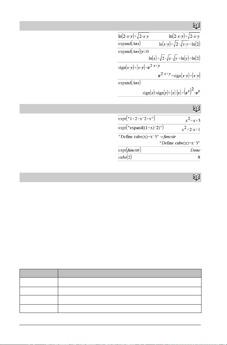
expand()
expand(Expr1,[Va r]) also distributes logarithms and fractional
powers regardless of Va r. For increased distr ibution of logarithms and
fractional powers, inequality constraints might be necessary to
guarantee that some factors are nonnegative.
expand(Expr1, [Va r]) also distributes absolute values, sign(),
and exponentials, regardless of Va r .
Note: See also tExpand() for trigonometric angle-sum and
multiple-angle expansion.
Catalog
>
expr()
expr(Stri ng) ⇒ expression
Returns the character string contained in Stri ng as an expression and
immediately executes it.
ExpReg
ExpReg X, Y [, [Freq] [, Category, Include]]
Computes the exponential regression y = a·(b)xon lists X and Y
with frequency Freq. A summary of results is stored in the
stat.results variable. (See page 105.)
All the lists must have equal dimension except for Include.
X and Y are lists of independent and dependent variables.
Freq is an optional list of frequency values. Each element in Freq
specifies the frequency of occurrence for each corresponding X and Y
data point. The default value is 1. All elements must be integers | 0.
Category is a list of numeric category codes for the corresponding X
and Y data.
Include is a list of one or more of the category codes. Only those data
items whose category code is included in this list are included in the
calculation.
Output variable Description
stat.RegEqn
Regression equation: a·(b)
x
stat.a, stat.b Regression coefficients
stat.r
2
Coefficient of linear determination for transformed data
stat.r Correlation coefficient for transformed data (x, ln(y))
Catalog
Catalog
>
>
40 TI-Nspire™ CAS Reference Guide
Page 47
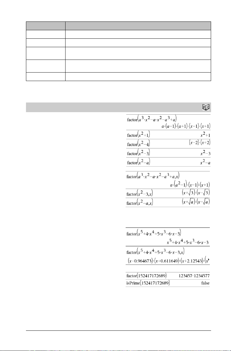
Output variable Description
stat.Resid Residuals associated with the exponential model
stat.ResidTrans Residuals associated with linear fit of transformed data
stat.XReg List of data points in the modified X List actually used in the regression based on restrictions of Freq,
stat.YReg List of data points in the modified Y List actually used in the regression based on restrictions of Freq,
stat.FreqReg List of frequencies corresponding to stat.XReg and stat.YReg
Category List, and Include Categories
Category List, and Include Categories
F
factor()
factor(Expr1[, Va r ]) ⇒ expression
factor(List1[,Va r ]) ⇒ list
factor(Matrix1[,Var ]) ⇒ matrix
factor(Expr1) returns Expr1 factored with respect to all of its
variables over a common denominator.
Expr1 is factored as much as possible toward linear rational factors
without introducing new non-real subexpressions. This alternative is
appropriate if you want factorization with respect to more than one
variable.
factor(Expr1,Var ) returns Expr1 factored with respect to variable
Var .
Expr1 is factored as much as possible toward real factors that are
linear in Va r, even if it introduces irrational constants or
subexpressions that are irrational in other variables.
The factors and their terms are sorted with Va r as the main variable.
Similar powers of Va r are collected in each factor. Include Va r if
factorization is needed with respect to only that variable and you are
willing to accept irrational expressions in any other variables to
increase factorization with respect to Va r . There might be some
incidental factoring with respect to other variables.
For the Auto setting of the Auto or Approximate mode,
including Va r permits approximation with floating-point coefficients
where irrational coefficients cannot be explicitly expressed concisely
in terms of the built-in functions. Even when there is only one
variable, including Va r might yield more complete factorization.
Note: See also comDenom() for a fast way to achieve partial
factoring when factor() is not fast enough or if it exhausts memory.
Note: See also cFactor() for factoring all the way to complex
coefficients in pursuit of linear factors.
factor(rationalNumber) returns the rational number factored into
primes. For composite numbers, the computing time grows
exponentially with the number of digits in the second-largest factor.
For example, factoring a 30-digit integer could take more than a day,
and factoring a 100-digit number could take more than a century.
Note: To stop (break) a computation, press w.
If you merely want to determine if a number is prime, use isPrime()
instead. It is much faster, particularly if rationalNumber is not prime
and if the second-largest factor has more than five digits.
Catalog
>
TI-Nspire™ CAS Reference Guide 41
Page 48

FCdf()
FCdf(lowBound,upBound,dfNumer,dfDenom) ⇒ number if
lowBound and upBound are numbers, list if lowBound and
upBound are lists
FCdf(lowBound,upBound,dfNumer,dfDenom) ⇒ number if
lowBound and upBound are numbers, list if lowBound and
upBound are lists
Computes the F distribution probability between lowBound and
upBound for the specified dfNumer (degrees of freedom) and
dfDenom.
upBound), set lowBound = 0.
For P(X
Catalog
>
Fill
Fill Expr, matrixVar ⇒ matrix
Replaces each element in variable matrixVar with Expr.
matrixVar must already exist.
Fill Expr, listVar ⇒ list
Replaces each element in variable listVar with Expr.
listVar must already exist.
FiveNumSummary
FiveNumSummary X[,[Freq][,Category,Include]]
Provides an abbreviated version of the 1-variable statistics on list X.
A summary of results is stored in the stat.results variable. (See page
105.)
X represents a list containing the data.
Freq is an optional list of frequency values. Each element in Freq
specifies the frequency of occurrence for each corresponding X value.
The default value is 1. All elements must be integers | 0.
Category is a list of numeric category codes for the corresponding X
values.
Include is a list of one or more of the category codes. Only those data
items whose category code is included in this list are included in the
calculation.
Output variable Description
stat.MinX Minimum of x values.
stat.Q1X 1st Quartile of x.
stat.MedianX Median of x.
stat.Q3X 3rd Quartile of x.
stat.MaxX Maximum of x values.
Catalog
Catalog
>
>
42 TI-Nspire™ CAS Reference Guide
Page 49

floor()
floor(Expr1) ⇒ integer
Returns the greatest integer that is { the argument. This function is
identical to int().
The argument can be a real or a complex number.
floor(List1) ⇒ list
floor(Matrix1) ⇒ matrix
Returns a list or matrix of the floor of each element.
Note: See also ceiling() and int().
Catalog
>
fMax()
fMax(Expr, Var) ⇒ Boolean expression
fMax(Expr, Va r,lowBound)
fMax(
Expr, Va r,lowBound,upBound)
fMax(
Expr, Va r) | lowBound<Va r <upBound
Returns a Boolean expression specifying candidate values of Va r that
maximize Expr or locate its least upper bound.
You can use the “|” operator to restrict the solution interval and/or
specify other constraints.
For the Approximate setting of the Auto or Approximate mode,
fMax() iteratively searches for one approximate local maximum.
This is often faster, particularly if you use the “|” operator to
constrain the search to a relatively small interval that contains exactly
one local maximum.
Note: See also fMin() and max().
fMin()
fMin(Expr, Var) ⇒ Boolean expression
fMin(Expr, Var ,lowBound)
fMin(
Expr, Va r,lowBound,upBound)
fMin(
Expr, Va r) | lowBound<Va r <upBound
Returns a Boolean expression specifying candidate values of Va r that
minimize Expr or locate its greatest lower bound.
You can use the “|” operator to restrict the solution interval and/or
specify other constraints.
For the Approximate setting of the Auto or Approximate mode,
fMin() iteratively searches for one approximate local minimum. This
is often faster, particularly if you use the “|” operator to constrain the
search to a relatively small interval that contains exactly one local
minimum.
Note: See also fMax() and min().
Catalog
Catalog
>
>
TI-Nspire™ CAS Reference Guide 43
Page 50

For
For Var , Low, High [, St ep]
Block
EndFor
Executes the statements in Block iteratively for each value of Va r ,
from Low to High, in increments of Step.
Var must not be a system variable.
Step can be positive or negative. The default value is 1.
Block can be either a single statement or a series of statements
separated with the “:” character.
Note for entering the example: In the Calculator application
on the handheld, you can enter multi-line definitions by pressing
@ instead of · at the end of each line. On the computer
keyboard, hold down Alt and press Enter.
Catalog
>
format()
format(Expr[, formatString]) ⇒ string
Returns Expr as a character string based on the format template.
Expr must simplify to a number.
formatString is a string and must be in the form: “F[n]”, “S[n]”,
“E[n]”, “G[n][c]”, where [ ] indicate optional portions.
F[n]: Fixed format. n is the number of digits to display after the
decimal point.
S[n]: Scientific format. n is the number of digits to display after the
decimal point.
E[n]: Engineering format. n is the number of digits after the first
significant digit. The exponent is adjusted to a multiple of three, and
the decimal point is moved to the right by zero, one, or two digits.
G[n][c]: Same as fixed format but also separates digits to the left of
the radix into groups of three. c specifies the group separator
character and defaults to a comma. If c is a period, the radix will be
shown as a comma.
[Rc]: Any of the above specifiers may be suffixed with the Rc radix
flag, where c is a single character that specifies what to substitute for
the radix point.
fPart()
fPart(Expr1) ⇒ expression
fPart(List1) ⇒ list
fPart(Matrix1) ⇒ matrix
Returns the fractional part of the argument.
For a list or matrix, returns the fractional parts of the elements.
The argument can be a real or a complex number.
FPdf()
FPdf(XVal,dfNumer,dfDenom) ⇒ number if XVal is a number,
list if XVal is a list
Computes the F distribution probability at XVal for the
specified dfNumer (degrees of freedom) and dfDenom.
Catalog
Catalog
Catalog
>
>
>
44 TI-Nspire™ CAS Reference Guide
Page 51

freqTable4list()
freqTable4list(List1,freqIntegerList) ⇒ list
Returns a list containing the elements from List1 expanded according
to the frequencies in freqIntegerList. This function can be used for
building a frequency table for the Data & Statistics application.
List1 can be any valid list.
freqIntegerList must have the same dimension as List1 and must
contain non-negative integer elements only. Each element specifies
the number of times the corresponding List1 element will be
repeated in the result list. A value of zero excludes the corresponding
List1 element.
Catalog
>
frequency()
frequency(List1,binsList) ⇒ list
Returns a list containing counts of the elements in List1. The counts
are based on ranges (bins) that you define in binsList.
If binsList is {b(1), b(2), …, b(n)}, the specified ranges are {?{b(1),
b(1)<?{b(2),…,b(n-1)<?{b(n), b(n)>?}. The resulting list is one
element longer than binsList.
Each element of the result corresponds to the number of elements
from List1 that are in the range of that bin. Expressed in terms of the
countIf() function, the result is { countIf(list, ?{b(1)), countIf(list,
b(1)<?{b(2)), …, countIf(list, b(n-1)<?{b(n)), countIf(list, b(n)>?)}.
Elements of List1 that cannot be “placed in a bin” are ignored.
Within the Lists & Spreadsheet application, you can use a range of
cells in place of both arguments.
Note: See also countIf(), page 23.
FTest_2Samp
FTest_2Samp List1,List2[,Freq1[,Freq2[,Hypoth]]]
FTest_2Samp
(Data list input)
List1,List2[,Freq1[,Freq2[,Hypoth]]]
FTest_2Samp sx1,n1,sx2,n2[,Hypoth]
FTest_2Samp
(Summary stats input)
Performs a two-sample F test. A summary of results is stored in the
stat.results variable. (See page 105.)
For Ha: s1 > s2, set Hypoth>0
For Ha: s1 ƒ s2 (default), set Hypoth =0
For Ha: s1 < s2, set Hypoth<0
sx1,n1,sx2,n2[,Hypoth]
Catalog
>
Explanation of result:
2 elements from Datalist are {2.5
4 elements from Datalist are >2.5 and {4.5
3 elements from Datalist are >4.5
The element "hello" is a string and cannot be placed in any of
the defined bins.
Catalog
>
Output variable Description
stat.F
stat.PVal Smallest level of significance at which the null hypothesis can be rejected
stat.dfNumer numerator degrees of freedom = n1-1
stat.dfDenom denominator degrees of freedom = n2-1
stat.sx1, stat.sx2 Sample standard deviations of the data sequences in List 1 and List 2
Calculated ó statistic for the data sequence
TI-Nspire™ CAS Reference Guide 45
Page 52

Output variable Description
stat.x1_bar
stat.x2_bar
stat.n1, stat.n2 Size of the samples
Sample means of the data sequences in List 1 and List 2
Func
Func
Block
EndFunc
Template for creating a user-defined function.
Block can be a single statement, a series of statements separated
with the “:” character, or a series of statements on separate lines.
The function can use the Return instruction to return a specific
result.
Note for entering the example: In the Calculator application
on the handheld, you can enter multi-line definitions by pressing
@ instead of · at the end of each line. On the computer
keyboard, hold down Alt and press Enter.
G
gcd()
gcd(Number1, Number2) ⇒ expression
Returns the greatest common divisor of the two arguments. The gcd
of two fractions is the gcd of their numerators divided by the lcm of
their denominators.
In Auto or Approximate mode, the gcd of fractional floating-point
numbers is 1.0.
gcd(List1, List2) ⇒ list
Returns the greatest common divisors of the corresponding elements
in List1 and List2.
gcd(Matrix1, Matrix2) ⇒ matrix
Returns the greatest common divisors of the corresponding elements
in Matrix1 and Matrix2.
Define a piecewise function:
Result of graphing g(x)
Catalog
Catalog
>
>
geomCdf()
geomCdf(p,lowBound,upBound) ⇒ number if lowBound and
upBound are numbers, list if lowBound and upBound are lists
geomCdf(
p,upBound) ⇒ number if upBound is a number, list
upBound is a list
if
Computes a cumulative geometric probability from lowBound to
upBound with the specified probability of success p.
For P(X upBound), set lowBound = 1.
Catalog
>
46 TI-Nspire™ CAS Reference Guide
Page 53

geomPdf()
geomPdf(p,XVal) ⇒ number if XVal is a number, list if XVal
is a list
Computes a probability at XVal, the number of the trial on which the
first success occurs, for the discrete geometric distribution with the
specified probability of success p.
Catalog
>
getDenom( )
getDenom(Expr1) ⇒ expression
Transforms the argument into an expression having a reduced
common denominator, and then returns its denominator.
getLangInfo( )
getLangInfo() ⇒ string
Returns a string that corresponds to the short name of the currently
active language. You can, for example, use it in a program or function
to determine the current language.
English = "en"
Danish = "da"
German = "de"
Finnish = "fi"
French = "fr"
Italian = "it"
Dutch = "nl"
Belgian Dutch = "nl_BE"
Norwegian = "no"
Portuguese = "pt"
Spanish = "es"
Swedish = "sv"
getMode()
getMode(ModeNameInteger) ⇒ value
getMode(0) ⇒ list
getMode(ModeNameInteger) returns a value representing the
current setting of the ModeNameInteger mode.
getMode(0) returns a list containing number pairs. Each pair
consists of a mode integer and a setting integer.
For a listing of the modes and their settings, refer to the table below.
If you save the settings with getMode(0) & var, you can use
setMode(var) in a function or program to temporarily restore the
settings within the execution of the function or program only. See
setMode(), page 96.
Catalog
Catalog
Catalog
>
>
>
TI-Nspire™ CAS Reference Guide 47
Page 54

Mode
Name
Mode
IntegerSetting Integers
Display Digits
Angle
Exponential Format
Real or Complex
Auto or Approx.
Vector Format
Base
Unit system
1
2
3
4
5
6
7
8
1
=Float, 2=Float1, 3=Float2, 4=Float3, 5=Float4, 6=Float5, 7=Float6, 8=Float7,
9=Float8, 10=Float9, 11=Float10, 12=Float11, 13=Float12, 14=Fix0, 15=Fix1,
16=Fix2, 17=Fix3, 18=Fix4, 19=Fix5, 20=Fix6, 21=Fix7, 22=Fix8, 23=Fix9, 24=Fix10,
25=Fix11, 26=Fix12
1
=Radian, 2=Degree, 3=Gradian
1
=Normal, 2=Scientific, 3=Engineering
1
=Real, 2=Rectangular, 3=Polar
1
=Auto, 2=Approximate, 3=Exact
1
=Rectangular, 2=Cylindrical, 3=Spherical
1
=Decimal, 2=Hex, 3=Binary
1
=SI, 2=Eng/US
getNum()
getNum(Expr1) ⇒ expression
Transforms the argument into an expression having a reduced
common denominator, and then returns its numerator.
getVarInfo()
getVarInfo() ⇒ matrix or string
getVarInfo(LibNameString) ⇒ matrix or string
getVarInfo() returns a matrix of information (variable name, type,
and library accessibility) for all variables and library objects defined in
the current problem.
If no variables are defined, getVarInfo() returns the string
"NONE".
getVarInfo(LibNameString) returns a matrix of information for
all library objects defined in library LibNameString. LibNameString
must be a string (text enclosed in quotation marks) or a string
variable.
If the library LibNameString does not exist, an error occurs.
Catalog
Catalog
>
>
48 TI-Nspire™ CAS Reference Guide
Page 55

getVarInfo()
Note the example to the left, in which the result of getVarInfo() is
assigned to variable vs. Attempting to display row 2 or row 3 of vs
returns an “Invalid list or matrix” error because at least one of
elements in those rows (variable b, for example) revaluates to a
matrix.
This error could also occur when using Ans to reevaluate a
getVarInfo() result.
The system gives the above error because the current version of the
software does not support a generalized matrix structure where an
element of a matrix can be either a matrix or a list.
Catalog
>
Goto
Goto labelName
Transfers control to the label labelName.
labelName must be defined in the same function using a Lbl
instruction.
Note for entering the example: In the Calculator application
on the handheld, you can enter multi-line definitions by pressing
@ instead of · at the end of each line. On the computer
keyboard, hold down Alt and press Enter.
4Grad
Expr1 4 Grad ⇒ expression
Converts Expr1 to gradian angle measure.
In Degree angle mode:
In Radian angle mode:
Catalog
Catalog
>
>
TI-Nspire™ CAS Reference Guide 49
Page 56

I
identity()
identity(Integer) ⇒ matrix
Returns the identity matrix with a dimension of Integer.
Integer must be a positive integer.
If
If BooleanExpr Statement
If BooleanExpr Then
Block
EndIf
If BooleanExpr evaluates to true, executes the single statement
Statement or the block of statements Block before continuing
execution.
If BooleanExpr evaluates to false, continues execution without
executing the statement or block of statements.
Block can be either a single statement or a sequence of statements
separated with the “:” character.
Note for entering the example: In the Calculator application
on the handheld, you can enter multi-line definitions by pressing
@ instead of · at the end of each line. On the computer
keyboard, hold down Alt and press Enter.
If BooleanExpr Then
Block1
Else
Block2
EndIf
If BooleanExpr evaluates to true, executes Block1 and then skips
Block2.
If BooleanExpr evaluates to false, skips Block1 but executes
Block2.
Block1 and Block2 can be a single statement.
Catalog
Catalog
>
>
50 TI-Nspire™ CAS Reference Guide
Page 57

If
If BooleanExpr1 Then
Block1
ElseIf
BooleanExpr2 Then
Block2
©
ElseIf
BooleanExprN Then
BlockN
EndIf
Allows for branching. If BooleanExpr1 evaluates to true, executes
Block1. If BooleanExpr1 evaluates to false, evaluates
BooleanExpr2, etc.
Catalog
>
ifFn()
ifFn(BooleanExpr,Val u e _ If _ t r ue [,Value_If_false
[,
Value_If_unknown]]) ⇒ expression, list, or matrix
Evaluates the boolean expression BooleanExpr (or each element
from BooleanExpr ) and produces a result based on the following
rules:
• BooleanExpr can test a single value, a list, or a matrix.
• If an element of BooleanExpr evaluates to true, returns the
corresponding element from Value_If_true.
• If an element of BooleanExpr evaluates to false, returns the
corresponding element from Value_If_false. If you omit
Value_If_false, returns undef.
• If an element of BooleanExpr is neither true nor false, returns
the corresponding element Value_If_unknown. If you omit
Value_If_unknown, returns undef.
• If the second, third, or fourth argument of the ifFn() function is
a single expression, the Boolean test is applied to every position
in BooleanExpr.
Note: If the simplified BooleanExpr statement involves a list or
matrix, all other list or matrix arguments must have the same
dimension(s), and the result will have the same dimension(s).
imag()
imag(Expr1) ⇒ expression
Returns the imaginary part of the argument.
Note: All undefined variables are treated as real variables. See also
real(), page 89
Catalog
>
Test va lue o f 1 is less than 2.5, so its corresponding
Value_If_True element of 5 is copied to the result list.
Test va lue o f 2 is less than 2.5, so its corresponding
Value_If_True element of 6 is copied to the result list.
Test va lue o f 3 is not less than 2.5, so its corresponding
Value_If_False element of 10 is copied to the result list.
Value_If_true is a single value and corresponds to any selected
position.
Value_If_false is not specified. Undef is used.
One element selected from Value_If_true. One element
selected from Value_If_unknown.
Catalog
>
imag(List1) ⇒ list
Returns a list of the imaginary parts of the elements.
TI-Nspire™ CAS Reference Guide 51
Page 58

imag()
imag(Matrix1) ⇒ matrix
Returns a matrix of the imaginary parts of the elements.
Catalog
>
impDif()
impDif(Equation, Va r, dependVar[,Ord])
⇒ expression
Catalog
>
where the order Ord defaults to 1.
Computes the implicit derivative for equations in which one variable
is defined implicitly in terms of another.
Indirection See #(), page 139.
inString()
inString(srcString, subString[, Start]) ⇒ integer
Returns the character position in string srcString at which the first
occurrence of string subString begins.
Start, if included, specifies the character position within srcString
where the search begins. Default = 1 (the first character of srcString).
If srcString does not contain subString or Start is > the length of
srcString, returns zero.
int()
int(Expr) ⇒ integer
int(List1) ⇒ list
int(Matrix1) ⇒ matrix
Returns the greatest integer that is less than or equal to the
argument. This function is identical to floor().
Catalog
Catalog
>
>
The argument can be a real or a complex number.
For a list or matrix, returns the greatest integer of each of the
elements.
intDiv()
intDiv(Number1, Number2) ⇒ integer
intDiv(List1, List2) ⇒ list
intDiv(Matrix1, Matrix2) ⇒ matrix
Catalog
>
Returns the signed integer part of (Number1 ÷ Number2).
For lists and matrices, returns the signed integer part of
(argument 1 ÷ argument 2) for each element pair.
integrate
‰
See
(), page 135.
52 TI-Nspire™ CAS Reference Guide
Page 59

invc2()
invc2(Area,df)
Area,df)
invChi2(
Computes the Inverse cumulative c2 (chi-square) probability function
specified by degree of freedom, df for a given Area under the curve.
Catalog
>
invF()
invF(Area,dfNumer,dfDenom)
Area,dfNumer,dfDenom)
invF(
computes the Inverse cumulative F distribution function specified by
dfNumer and dfDenom for a given Area under the curve.
invNorm()
invNorm(Area[,m[,s]])
Computes the inverse cumulative normal distribution function for a
given Area under the normal distribution curve specified by m and s.
invt()
invt(Area,df)
Computes the inverse cumulative student-t probability function
specified by degree of freedom, df for a given Area under the curve.
iPart()
iPart(Number) ⇒ integer
iPart(List1) ⇒ list
iPart(Matrix1) ⇒ matrix
Returns the integer part of the argument.
For lists and matrices, returns the integer part of each element.
The argument can be a real or a complex number.
irr()
irr(CF0,CFList [,CFFreq]) ⇒ value
Financial function that calculates internal rate of return of an
investment.
CF0 is the initial cash flow at time 0; it must be a real number.
CFList is a list of cash flow amounts after the initial cash flow CF0.
CFFreq is an optional list in which each element specifies the
frequency of occurrence for a grouped (consecutive) cash flow
amount, which is the corresponding element of CFList. The default is
1; if you enter values, they must be positive integers < 10,000.
Note: See also mirr(), page 68.
Catalog
Catalog
Catalog
Catalog
Catalog
>
>
>
>
>
TI-Nspire™ CAS Reference Guide 53
Page 60
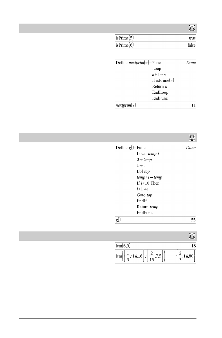
isPrime()
isPrime(Number) ⇒ Boolean constant expression
Returns true or false to indicate if number is a whole number ‚ 2 that
is evenly divisible only by itself and 1.
If Number exceeds about 306 digits and has no factors
isPrime(Number) displays an error message.
If you merely want to determine if Number is prime, use
instead of
factor(). It is much faster, particularly if Number is not
prime and has a second-largest factor that exceeds about five digits.
Note for entering the example: In the Calculator application
on the handheld, you can enter multi-line definitions by pressing
{1021,
isPrime()
@ instead of · at the end of each line. On the computer
keyboard, hold down Alt and press Enter.
L
Catalog
Function to find the next prime after a specified number:
>
Lbl
Lbl labelName
Defines a label with the name labelName within a function.
You can use a Goto labelName instruction to transfer control to the
instruction immediately following the label.
labelName must meet the same naming requirements as a variable
name.
Note for entering the example: In the Calculator application
on the handheld, you can enter multi-line definitions by pressing
@ instead of · at the end of each line. On the computer
keyboard, hold down Alt and press Enter.
lcm()
lcm(Number1, Number2) ⇒ expression
lcm(List1, List2) ⇒ list
lcm(Matrix1, Matrix2) ⇒ matrix
Returns the least common multiple of the two arguments. The lcm of
two fractions is the lcm of their numerators divided by the gcd of
their denominators. The lcm of fractional floating-point numbers is
their product.
For two lists or matrices, returns the least common multiples of the
corresponding elements.
Catalog
Catalog
>
>
54 TI-Nspire™ CAS Reference Guide
Page 61

left()
left(sourceString[, Num]) ⇒ string
Returns the leftmost Num characters contained in character string
sourceString.
If you omit Num, returns all of sourceString.
left(List1[, Num]) ⇒ list
Returns the leftmost Num elements contained in List1.
If you omit Num, returns all of List1.
left(Comparison) ⇒ expression
Returns the left-hand side of an equation or inequality.
Catalog
>
libShortcut()
libShortcut(LibNameString, ShortcutNameString
[, LibPrivFlag]) ⇒ list of variables
Creates a variable group in the current problem that contains
references to all the objects in the specified library document
libNameString. Also adds the group members to the Variables menu.
You can then refer to each object using its ShortcutNameString.
Set LibPrivFlag=0 to exclude private library objects (default)
Set LibPrivFlag=1 to include private library objects
To copy a variable group, see CopyVar on page 18.
To delete a variable group, see DelVar on page 31.
limit() or lim()
limit(Expr1, Va r, Point [,Direction]) ⇒ expression
limit(List1, Va r, Point [, Direction]) ⇒ list
limit(Matrix1, Var , Point [, Direction]) ⇒ matrix
Returns the limit requested.
Note: See also Limit template, page 5.
Direction: negative=from left, positive=from right, otherwise=both.
(If omitted, Direction defaults to both.)
Catalog
>
This example assumes a properly stored and refreshed library
document named linalg2 that contains objects defined as
clearmat, gauss1, and gauss2.
Catalog
>
Limits at positive ˆ and at negative ˆ are always converted to onesided limits from the finite side.
Depending on the circumstances, limit() returns it self or undef when
it cannot determine a unique limit. This does not necessarily mean
that a unique limit does not exist. undef means that the result is
either an unknown number with finite or infinite magnitude, or it is
the entire set of such numbers.
TI-Nspire™ CAS Reference Guide 55
Page 62

limit() or lim()
limit() uses methods such as L’Hopital’s rule, so there are unique
limits that it cannot determine. If Expr1 contains undefined variables
other than Va r, you might have to constrain them to obtain a more
concise result.
Limits can be very sensitive to rounding error. When possible, avoid
the Approximate setting of the Auto or Approximate mode and
approximate numbers when computing limits. Otherwise, limits that
should be zero or have infinite magnitude probably will not, and
limits that should have finite non-zero magnitude might not.
Catalog
>
LinRegBx
LinRegBx X,Y[,[Freq][,Category,Include]]
Computes the linear regression y = a+b·x on lists X and Y with
frequency Freq. A summary of results is stored in the stat.results
variable. (See page 105.)
All the lists must have equal dimension except for Include.
X and Y are lists of independent and dependent variables.
Freq is an optional list of frequency values. Each element in Freq
specifies the frequency of occurrence for each corresponding X and Y
data point. The default value is 1. All elements must be integers | 0.
Category is a list of numeric category codes for the corresponding X
and Y data.
Include is a list of one or more of the category codes. Only those data
items whose category code is included in this list are included in the
calculation.
Output variable Description
stat.RegEqn
stat.a, stat.b Regression coefficients
2
stat.r
stat.r Correlation coefficient
stat.Resid Residuals from the regression
stat.XReg List of data points in the modified X List actually used in the regression based on restrictions of Freq,
stat.YReg List of data points in the modified Y List actually used in the regression based on restrictions of Freq,
stat.FreqReg List of frequencies corresponding to stat.FreqReg and stat.YReg
Regression Equation: a+b·x
Coefficient of determination
Category List, and Include Categories
Category List, and Include Categories
Catalog
>
56 TI-Nspire™ CAS Reference Guide
Page 63

LinRegMx
LinRegMx X,Y[,[Freq][,Category,Include]]
Computes the linear regression y = m·x+b on lists X and Y with
frequency Freq. A summary of results is stored in the stat.results
variable. (See page 105.)
Catalog
All the lists must have equal dimension except for Include.
X and Y are lists of independent and dependent variables.
Freq is an optional list of frequency values. Each element in Freq
specifies the frequency of occurrence for each corresponding X and Y
data point. The default value is 1. All elements must be integers | 0.
Category is a list of numeric category codes for the corresponding X
and Y data.
Include is a list of one or more of the category codes. Only those data
items whose category code is included in this list are included in the
calculation.
Output variable Description
stat.RegEqn
Regression Equation: m·x+b
stat.m, stat.b Regression coefficients
stat.r
2
Coefficient of determination
stat.r Correlation coefficient
stat.Resid Residuals from the regression
stat.XReg List of data points in the modified X List actually used in the regression based on restrictions of Freq,
stat.YReg List of data points in the modified Y List actually used in the regression based on restrictions of Freq,
Category List, and Include Categories
Category List, and Include Categories
stat.FreqReg List of frequencies corresponding to stat.XReg and stat.YReg
>
LinRegtIntervals
LinRegtIntervals X,Y[,Freq[,0[,CLev]]]
Catalog
>
For Slope. Computes a level C confidence interval for the slope.
LinRegtIntervals X,Y[,Freq[,1,Xval[,CLev]]]
For Response. Computes a predicted y-value, a level C prediction
interval for a single observation, and a level C confidence interval for
the mean response.
A summary of results is stored in the stat.results variable. (See page
105.)
All the lists must have equal dimension.
X and Y are lists of independent and dependent variables.
Freq is an optional list of frequency values. Each element in Freq
specifies the frequency of occurrence for each corresponding X and Y
data point. The default value is 1. All elements must be integers | 0.
TI-Nspire™ CAS Reference Guide 57
Page 64

Output variable Description
stat.RegEqn
stat.a, stat.b Regression coefficients
stat.df Degrees of freedom
2
stat.r
stat.r Correlation coefficient
stat.Resid Residuals from the regression
For Slope type only
Output variable Description
[stat.CLower,
stat.CUpper]
stat.ME Confidence interval margin of error
stat.SESlope Standard error of slope
stat.s Standard error about the line
For Response type only
Output variable Description
[stat.CLower,
stat.CUpper]
stat.ME Confidence interval margin of error
stat.SE Standard error of mean response
[stat.LowerPred ,
stat.UpperPred]
stat.MEPred Prediction interval margin of error
stat.SEPred Standard error for prediction
stat.y
Regression Equation: a+b
Coefficient of determination
Confidence interval for the slope
Confidence interval for the mean response
Prediction interval for a single observation
a + b·XVal
·x
58 TI-Nspire™ CAS Reference Guide
Page 65

LinRegtTest
LinRegtTest X,Y[,Freq[,Hypoth]]
Computes a linear regression on the X and Y lists and a t test on the
value of slope b and the correlation coefficient r for the equation
y=a+bx. It tests the null hypothesis H0:b=0 (equivalently, r=0)
against one of three alternative hypotheses.
All the lists must have equal dimension.
X and Y are lists of independent and dependent variables.
Freq is an optional list of frequency values. Each element in Freq
specifies the frequency of occurrence for each corresponding X and Y
data point. The default value is 1. All elements must be integers | 0.
Hypoth is an optional value specifying one of three alternative
hypotheses against which the null hypothesis (H0:b=r=0) will be
tested.
For Ha: bƒ0 and rƒ0 (default), set Hypoth=0
For Ha: b<0 and r<0, set Hypoth<0
For Ha: b>0 and r>0, set Hypoth>0
A summary of results is stored in the stat.results variable. (See page
105.)
Output variable Description
stat.RegEqn
stat.t t-Statistic for significance test
stat.PVal Smallest level of significance at which the null hypothesis can be rejected
stat.df Degrees of freedom
stat.a, stat.b Regression coefficients
stat.s Standard error about the line
stat.SESlope Standard error of slope
2
stat.r
stat.r Correlation coefficient
stat.Resid Residuals from the regression
Regression equation: a + b·x
Coefficient of determination
Catalog
>
@List()
Catalog
>
@List(List1) ⇒ list
Returns a list containing the differences between consecutive
elements in List1. Each element of List1 is subtracted from the next
element of List1. The resulting list is always one element shorter than
the original List1.
TI-Nspire™ CAS Reference Guide 59
Page 66

list4mat()
list4mat(List [, elementsPerRow]) ⇒ matrix
Returns a matrix filled row-by-row with the elements from List.
elementsPerRow, if included, specifies the number of elements per
row. Default is the number of elements in List (one row).
If List does not fill the resulting matrix, zeros are added.
Catalog
>
4ln
Expr 4ln ⇒ expression
Causes the input Expr to be converted to an expression containing
only natural logs (ln).
ln()
ln(Expr1) ⇒ expression
ln(List1) ⇒ list
Returns the natural logarithm of the argument.
For a list, returns the natural logarithms of the elements.
ln(squareMatrix1) ⇒ squareMatrix
Returns the matrix natural logarithm of squareMatrix1. This is not
the same as calculating the natural logarithm of each element. For
information about the calculation method, refer to cos() on.
squareMatrix1 must be diagonalizable. The result always contains
floating-point numbers.
Catalog
>
/u
If complex format mode is Real:
If complex format mode is Rectangular:
In Radian angle mode and Rectangular complex format:
To see the entire result, press £ and then use ¡ and ¢ to
move the cursor.
keys
60 TI-Nspire™ CAS Reference Guide
Page 67

LnReg
LnReg X, Y[, [Freq] [, Category, Include]]
Computes the logarithmic regression y = a+b·ln(x) on lists X and Y
with frequency Freq. A summary of results is stored in the
stat.results variable. (See page 105.)
All the lists must have equal dimension except for Include.
X and Y are lists of independent and dependent variables.
Freq is an optional list of frequency values. Each element in Freq
specifies the frequency of occurrence for each corresponding X and Y
data point. The default value is 1. All elements must be integers | 0.
Category is a list of numeric category codes for the corresponding X
and Y data.
Include is a list of one or more of the category codes. Only those data
items whose category code is included in this list are included in the
calculation.
Output variable Description
stat.RegEqn
stat.a, stat.b Regression coefficients
2
stat.r
stat.r Correlation coefficient for transformed data (ln(x), y)
stat.Resid Residuals associated with the logarithmic model
stat.ResidTrans Residuals associated with linear fit of transformed data
stat.XReg List of data points in the modified X List actually used in the regression based on restrictions of Freq,
stat.YReg List of data points in the modified Y List actually used in the regression based on restrictions of Freq,
stat.FreqReg List of frequencies corresponding to stat.XReg and stat.YReg
Regression equation: a+b·ln(x)
Coefficient of linear determination for transformed data
Category List, and Include Categories
Category List, and Include Categories
Catalog
>
Local
Local Var 1 [, Va r 2] [, Va r 3 ] ...
Declares the specified vars as local variables. Those variables exist
only during evaluation of a function and are deleted when the
function finishes execution.
Note: Local variables save memory because they only exist
temporarily. Also, they do not disturb any existing global variable
values. Local variables must be used for For loops and for
temporarily saving values in a multi-line function since modifications
on global variables are not allowed in a function.
Note for entering the example: In the Calculator application
on the handheld, you can enter multi-line definitions by pressing
Catalog
>
@ instead of · at the end of each line. On the computer
keyboard, hold down Alt and press Enter.
TI-Nspire™ CAS Reference Guide 61
Page 68

log()
log(Expr1[,Expr2]) ⇒ expression
log(List1[,Expr2]) ⇒ list
Returns the base-Expr2 logarithm of the first argument.
Note: See also Log template, page 2.
For a list, returns the base-Expr2 logarithm of the elements.
If the second argument is omitted, 10 is used as the base.
If complex format mode is Real:
If complex format mode is Rectangular:
/
s
keys
log(squareMatrix1[,Expr]) ⇒ squareMatrix
Returns the matrix base-Expr logarithm of squareMatrix1. This is
not the same as calculating the base-Expr logarithm of each element.
For information about the calculation method, refer to cos().
squareMatrix1 must be diagonalizable. The result always contains
floating-point numbers.
If the base argument is omitted, 10 is used as base.
4logbase
Expr 4logbase(Expr1) ⇒ expression
Causes the input Expression to be simplified to an expression using
base Expr1.
In Radian angle mode and Rectangular complex format:
To see the entire result, press £ and then use ¡ and ¢ to
move the cursor.
Catalog
>
62 TI-Nspire™ CAS Reference Guide
Page 69

Logistic
Logistic X, Y[, [Freq] [, Category, Include]]
Computes the logistic regression y = (c/(1+a·e
with frequency Freq. A summary of results is stored in the
stat.results variable. (See page 105.)
-bx
)) on lists X and Y
Catalog
All the lists must have equal dimension except for Include.
X and Y are lists of independent and dependent variables.
Freq is an optional list of frequency values. Each element in Freq
specifies the frequency of occurrence for each corresponding X and Y
data point. The default value is 1. All elements must be integers | 0.
Category is a list of numeric category codes for the corresponding X
and Y data.
Include is a list of one or more of the category codes. Only those data
items whose category code is included in this list are included in the
calculation.
Output variable Description
stat.RegEqn
Regression equation: c/(1+a·e
-bx
)
stat.a, stat.b, stat.c Regression coefficients
stat.Resid Residuals from the regression
stat.XReg List of data points in the modified X List actually used in the regression based on restrictions of Freq,
stat.YReg List of data points in the modified Y List actually used in the regression based on restrictions of Freq,
Category List, and Include Categories
Category List, and Include Categories
stat.FreqReg List of frequencies corresponding to stat.XReg and stat.YReg
>
LogisticD
LogisticD X, Y [ , [Iterations] , [Freq] [, Category, Include] ]
Computes the logistic regression y = (c/(1+a·e
Y with frequency Freq, using a specified number of Iterations. A
summary of results is stored in the stat.results variable. (See page
105.)
-bx
)+d) on lists X and
Catalog
>
All the lists must have equal dimension except for Include.
X and Y are lists of independent and dependent variables.
Iterations is an optional value that specifies the maximum number of
times a solution will be attempted. If omitted, 64 is used. Typically,
larger values result in better accuracy but longer exe cution times, and
vice versa.
Freq is an optional list of frequency values. Each element in Freq
specifies the frequency of occurrence for each corresponding X and Y
data point. The default value is 1. All elements must be integers | 0.
Category is a list of numeric category codes for the corresponding X
and Y data.
Include is a list of one or more of the category codes. Only those data
items whose category code is included in this list are included in the
calculation.
TI-Nspire™ CAS Reference Guide 63
Page 70

Output variable Description
stat.RegEqn
stat.a, stat.b, stat.c,
stat.d
stat.Resid Residuals from the regression
stat.XReg List of data points in the modified X List actually used in the regression based on restrictions of Freq,
stat.YReg List of data points in the modified Y List actually used in the regression based on restrictions of Freq,
stat.FreqReg List of frequencies corresponding to stat.XReg and stat.YReg
Regression equation: c/(1+a·e
Regression coefficients
Category List, and Include Categories
Category List, and Include Categories
-bx
)+d)
Loop
Loop
Block
EndLoop
Repeatedly executes the statements in Block. Note that the loop will
be executed endlessly, unless a Goto or Exit instruction is executed
within Block.
Block is a sequence of statements separated with the “:” character.
Note for entering the example: In the Calculator application
on the handheld, you can enter multi-line definitions by pressing
@ instead of · at the end of each line. On the computer
keyboard, hold down Alt and press Enter.
Catalog
>
64 TI-Nspire™ CAS Reference Guide
Page 71

LU
LU Matrix, lMatName, uMatName, pMatName[, Tol ]
Calculates the Doolittle LU (lower-upper) decomposition of a real or
complex matrix. The lower triangular matrix is stored in lMatName,
the upper triangular matrix in uMatName, and the permutation
matrix (which describes the row swaps done during the calculation) in
pMatName.
lMatName · uMatName = pMatName · matrix
Optionally, any matrix element is treated as zero if its absolute value
is less than Tol . This tolerance is used only if the matrix has floatingpoint entries and does not contain any symbolic variables that have
not been assigned a value. Otherwise, To l is ignored.
• If you use
•If Tol is omitted or not used, the default tolerance is calculated
The LU factorization algorithm uses partial pivoting with row
interchanges.
/
mode to Approximate, computations are done using floatingpoint arithmetic.
as:
5EM14 ·max(dim(Matrix)) ·rowNorm(Matrix)
· or set the Auto or Approximate
Catalog
>
M
mat4list()
mat4list(Matrix) ⇒ list
Returns a list filled with the elements in Matrix. The elements are
copied from Matrix row by row.
TI-Nspire™ CAS Reference Guide 65
Catalog
>
Page 72

max()
max(Expr1, Expr2) ⇒ expression
max(List1, List2) ⇒ list
max(Matrix1, Matrix2) ⇒ matrix
Returns the maximum of the two arguments. If the arguments are
two lists or matrices, returns a list or matrix containing the maximum
value of each pair of corresponding elements.
max(List) ⇒ expression
Returns the maximum element in list.
max(Matrix1) ⇒ matrix
Returns a row vector containing the maximum element of each
column in Matrix1.
Note: See also fMax() and min().
Catalog
>
mean()
mean(List[, freqList]) ⇒ expression
Returns the mean of the elements in List.
Each freqList element counts the number of consecutive occurrences
of the corresponding element in List.
mean(Matrix1[, freqMatrix]) ⇒ matrix
Returns a row vector of the means of all the columns in Matrix1.
Each freqMatrix element counts the number of consecutive
occurrences of the corresponding element in Matrix1.
median()
median(List) ⇒ expression
Returns the median of the elements in List.
median(Matrix1) ⇒ matrix
Returns a row vector containing the medians of the columns in
Matrix1.
Note: All entries in the list or matrix must simplify to numbers.
In Rectangular vector format:
Catalog
Catalog
>
>
66 TI-Nspire™ CAS Reference Guide
Page 73

MedMed
MedMed X,Y [, Freq] [, Category, Include]]
Computes the median-median line y = (m·x+b) on lists X and Y
with frequency Freq. A summary of results is stored in the
stat.results variable. (See page 105.)
All the lists must have equal dimension except for Include.
X and Y are lists of independent and dependent variables.
Freq is an optional list of frequency values. Each element in Freq
specifies the frequency of occurrence for each corresponding X and Y
data point. The default value is 1. All elements must be integers | 0.
Category is a list of numeric category codes for the corresponding X
and Y data.
Include is a list of one or more of the category codes. Only those data
items whose category code is included in this list are included in the
calculation.
Output variable Description
stat.RegEqn
stat.m, stat.b Model coefficients
stat.Resid Residuals from the median-median line
stat.XReg List of data points in the modified X List actually used in the regression based on restrictions of Freq,
stat.YReg List of data points in the modified Y List actually used in the regression based on restrictions of Freq,
stat.FreqReg List of frequencies corresponding to stat.XReg and stat.YReg
Median-median line equation: m·x+b
Category List, and Include Categories
Category List, and Include Categories
Catalog
>
mid()
mid(sourceString, Start[, Count]) ⇒ string
Returns Count characters from character string sourceString,
beginning with character number Star t.
If Count is omitted or is greater than the dimension of sourceString,
returns all characters from sourceString, beginning with character
number Start.
Count must be ‚ 0. If Count = 0, returns an empty string.
mid(sourceList, Start [, Count]) ⇒ list
Returns Count elements from sourceList, beginning with element
number Start.
If Count is omitted or is greater than the dimension of sourceList,
returns all elements from sourceList, beginning with element number
Start.
Count must be ‚ 0. If Count = 0, returns an empty list.
mid(sourceStringList, Start[, Count]) ⇒ list
Returns Count strings from the list of strings sourceStringList,
beginning with element number Start.
Catalog
>
TI-Nspire™ CAS Reference Guide 67
Page 74

min()
min(Expr1, Expr2) ⇒ expression
min(List1, List2) ⇒ list
min(Matrix1, Matrix2) ⇒ matrix
Returns the minimum of the two arguments. If the arguments are two
lists or matrices, returns a list or matrix containing the minimum
value of each pair of corresponding elements.
min(List) ⇒ expression
Returns the minimum element of List.
min(Matrix1) ⇒ matrix
Returns a row vector containing the minimum element of each
column in Matrix1.
Note: See also fMin() and max().
Catalog
>
mirr()
mirr(financeRate,reinvestRate,CF0,CFList[,CFFreq])
Financial function that returns the modified internal rate of return of
an investment.
financeRate is the interest rate that you pay on the cash flow
amounts.
rein vestRa te is the interest rate at which the cash flows are
reinvested.
CF0 is the initial cash flow at time 0; it must be a real number.
CFList is a list of cash flow amounts after the initial cash flow CF0.
CFFreq is an optional list in which each element specifies the
frequency of occurrence for a grouped (consecutive) cash flow
amount, which is the corresponding element of CFList. The default is
1; if you enter values, they must be positive integers < 10,000.
Note: See also irr(), page 53.
mod()
mod(Expr1, Expr2) ⇒ expression
mod(List1, List2) ⇒ list
mod(Matrix1, Matrix2) ⇒ matrix
Returns the first argument modulo the second argument as defined
by the identities:
mod(x,0) = x
mod(x,y) = x -ìy floor(x/y)
When the second argument is non-zero, the result is periodic in that
argument. The result is either zero or has the same sign as the second
argument.
If the arguments are two lists or two matrices, returns a list or matrix
containing the modulo of each pair of corresponding elements.
Note: See also remain(), page 90
Catalog
Catalog
>
>
mRow()
mRow(Expr, Matrix1, Index) ⇒ matrix
Returns a copy of Matrix1 with each element in row Index of
Matrix1 multiplied by Expr.
Catalog
>
68 TI-Nspire™ CAS Reference Guide
Page 75

mRowAdd()
mRowAdd(Expr, Matrix1, Index1, Index2) ⇒ matrix
Returns a copy of Matrix1 with each element in row Index2 of
Matrix1 replaced with:
Expr · row Index1 + row Index2
Catalog
>
MultReg
MultReg Y, X1[,X2[,X3,…[,X10]]]
Calculates multiple linear regression of list Y on lists X1, X2, …, X10.
A summary of results is stored in the stat.results variable. (See page
105.)
All the lists must have equal dimension.
Output variable Description
stat.RegEqn
Regression Equation: b0+b1·x1+b2·x2+ ...
stat.b0, stat.b1, ... Regression coefficients
stat.R
2
Coefficient of multiple determination
stat.yList yList = b0+b1·x1+ ...
stat.Resid Residuals from the regression
MultRegIntervals
MultRegIntervals Y, X1[,X2[,X3,…[,X10]]],XValList[,CLevel]
Computes a predicted y-value, a level C prediction interval for a single
observation, and a level C confidence interval for the mean response.
A summary of results is stored in the stat.results variable. (See page
105.)
All the lists must have equal dimension.
Output variable Description
stat.RegEqn
Regression Equation: b0+b1·x1+b2·x2+ ...
Catalog
Catalog
>
>
stat.y A point estimate: y = b0 + b1 · xl + ... for XValList
stat.dfError Error degrees of freedom
stat.CLower, stat.CUpper Confidence interval for a mean response
stat.ME Confidence interval margin of error
stat.SE Standard error of mean response
stat.LowerPred,
stat.UpperrPred
Prediction interval for a single observation
TI-Nspire™ CAS Reference Guide 69
Page 76

Output variable Description
stat.MEPred Prediction interval margin of error
stat.SEPred Standard error for prediction
stat.bList List of regression coefficients, {b0,b1,b2,...}
stat.Resid Residuals from the regression
MultRegTests
MultRegTests Y, X1[,X2[,X3,…[,X10]]]
Multiple linear regression test computes a multiple linear regression
on the given data and provides the global F test statistic and t test
statistics for the coefficients.
A summary of results is stored in the stat.results variable. (See page
105.)
Catalog
Outputs
Output variable Description
stat.RegEqn
Regression Equation: b0+b1·x1+b2·x2+ ...
stat.F Global F test statistic
stat.PVal P-value associated with global F statistic
stat.R
stat.AdjR
2
2
Coefficient of multiple determination
Adjusted coefficient of multiple determination
stat.s Standard deviation of the error
stat.DW Durbin-Watson statistic; used to determine whether first-order auto correlation is present in the model
stat.dfReg Regression degrees of freedom
stat.SSReg Regression sum of squares
stat.MSReg Regression mean square
stat.dfError Error degrees of freedom
stat.SSError Error sum of squares
stat.MSError Error mean square
stat.bList {b0,b1,...} List of coefficients
stat.tList List of t statistics, one for each coefficient in the bList
stat.PList List P-values for each t statistic
stat.SEList List of standard errors for coefficients in bList
>
stat.yList yList = b0+b1·x1+...
stat.Resid Residuals from the regression
stat.sResid Standardized residuals; obtained by dividing a residual by its standard deviation
stat.CookDist Cook’s distance; measure of the influence of an observation based on the residual and leverage
70 TI-Nspire™ CAS Reference Guide
Page 77

Output variable Description
stat.Leverage Measure of how far the values of the independent variable are from their mean values
N
nCr()
nCr(Expr1, Expr2) ⇒ expression
For integer Expr1 and Expr2 with Expr1 ‚ Expr2 ‚ 0, nCr() is the
number of combinations of Expr1 things taken Expr2 at a time. (This
is also known as a binomial coefficient.) Both arguments can be
integers or symbolic expressions.
nCr(Expr, 0) ⇒ 1
Expr, negInteger) ⇒ 0
nCr(
Expr, posInteger) ⇒ Expr·(ExprN1)...
nCr(
ExprNposInteger+1)/ posInteger!
(
Expr, nonInteger) ⇒ expression!/
nCr(
((
ExprNnonInteger)!·nonInteger!)
List1, List2) ⇒ list
nCr(
Returns a list of combinations based on the corresponding element
pairs in the two lists. The arguments must be the same size list.
nCr(Matrix1, Matrix2) ⇒ matrix
Returns a matrix of combinations based on the corresponding
element pairs in the two matrices. The arguments must be the same
size matrix.
nDeriv()
nDeriv(Expr1, Va r [=Value] [, H]) ⇒ expression
nDeriv(Expr1, Va r [, H] | Var = Va lu e ) ⇒ expression
nDeriv(Expr1, Va r [=Value], List) ⇒ list
nDeriv(List1, Va r [=Value] [, H]) ⇒ list
nDeriv(Matrix1, Va r [=Value] [, H]) ⇒ matrix
Returns the numerical derivative as an expression. Uses the central
difference quotient formula.
When Val u e is specified, it overrides any prior variable assignment or
any current “such that” substitution for the variable.
H is the step value. If H is omitted, it defaults to 0.001.
When using List1 or Matrix1, the operation gets mapped across the
values in the list or across the matrix elements.
Note: See also avgRC() and d().
Catalog
Catalog
>
>
newList()
newList(numElements) ⇒ list
Returns a list with a dimension of numElements. Each element is
zero.
Catalog
>
TI-Nspire™ CAS Reference Guide 71
Page 78

newMat()
newMat(numRows, numColumns) ⇒ matrix
Returns a matrix of zeros with the dimension numRows by
numColumns.
Catalog
>
nfMax()
nfMax(Expr, Va r) ⇒ value
nfMax(Expr, Va r, lowBound) ⇒ value
nfMax(Expr, Va r, lowBound, upBound) ⇒ value
nfMax(Expr, Var) | lowBound<Var <upBound ⇒ value
Returns a candidate numerical value of variable Va r where the local
maximum of Expr occurs.
If you supply lowBound and upBound, the function looks between
those values for the local maximum.
Note: See also fMax() and d().
nfMin()
nfMin(Expr, Va r) ⇒ value
nfMin(Expr, Va r, lowBound) ⇒ value
nfMin(Expr, Va r, lowBound, upBound) ⇒ value
nfMin(Expr, Var) | lowBound<Var <upBound ⇒ value
Returns a candidate numerical value of variable Va r where the local
minimum of Expr occurs.
If you supply lowBound and upBound, the function looks between
those values for the local minimum.
Note: See also fMin() and d().
nInt()
nInt(Expr1, Var, Lower, Upper) ⇒ expression
If the integrand Expr1 contains no variable other than Va r , and if
Lower and Upper are constants, positive ˆ, or negative ˆ, then
nInt() returns an approximation of ‰(Expr1, Va r , Lower, Upper).
This approximation is a weighted average of some sample values of
the integrand in the interval Lower<Va r <Upper.
The goal is six significant digits. The adaptive algorithm terminates
when it seems likely that the goal has been achieved, or when it
seems unlikely that additional samples will yield a worthwhile
improvement.
A warning is displayed (“Questionable accuracy”) when it seems that
the goal has not been achieved.
Catalog
Catalog
Catalog
>
>
>
Nest nInt() to do multiple numeric integration. Integration limits can
depend on integration variables outside them.
Note: See also ‰(), page 135.
72 TI-Nspire™ CAS Reference Guide
Page 79

nom()
nom(effectiveRate,CpY) ⇒ value
Financial function that converts the annual effective interest rate
effectiveRate to a nominal rate, given CpY as the number of
compounding periods per year.
effectiveRate must be a real number, and CpY must be a real number
> 0.
Note: See also eff(), page 36.
Catalog
>
norm()
norm(Matrix) ⇒ expression
norm(Ve c to r ) ⇒ expression
Returns the Frobenius norm.
normalLine()
normalLine(Expr1,Va r ,Point) ⇒ expression
normalLine(Expr1,Va r =Point) ⇒ expression
Returns the normal line to the curve represented by Expr1 at the
point specified in Va r=Point.
Make sure that the independent variable is not defined. For example,
If f1(x):=5 and x:=3, then normalLine(f1(x),x,2) returns "false."
normCdf()
normCdf(lowBound,upBound[,m[,s]]) ⇒ number if lowBound
upBound are numbers, list if lowBound and upBound are
and
lists
Computes the normal distribution probability between lowBound
and upBound for the specified m (default=0) and s (default=1).
For P(X upBound), set lowBound = .ˆ.
Catalog
Catalog
Catalog
>
>
>
normPdf()
normPdf(XVal[,m[,s]]) ⇒ number if XVal is a number, list if
XVal is a list
Computes the probability density function for the normal distribution
at a specified XVal value for the specified m and s.
Catalog
>
TI-Nspire™ CAS Reference Guide 73
Page 80

not
not BooleanExpr ⇒ Boolean expression
Returns true, false, or a simplified form of the argument.
Catalog
>
not Integer1 ⇒ integer
Returns the one’s complement of a real integer. Internally, Integer1 is
converted to a signed, 64-bit binary number. The value of each bit is
flipped (0 becomes 1, and vice versa) for the one’s complement.
Results are displayed according to the Base mode.
You can enter the integer in any number base. For a binary or
hexadecimal entry, you must use the 0b or 0h prefix, respectively.
Without a prefix, the integer is treated as decimal (base 10).
If you enter a decimal integer that is too large for a signed, 64-bit
binary form, a symmetric modulo operation is used to bring the value
into the appropriate range.
nPr()
nPr(Expr1, Expr2) ⇒ expression
For integer Expr1 and Expr2 with Expr1 ‚ Expr2 ‚ 0, nPr() is the
number of permutations of Expr1 things taken Expr2 at a time. Both
arguments can be integers or symbolic expressions.
nPr(Expr, 0) ⇒ 1
Expr, negInteger) ⇒ 1/((Expr+1)·(Expr+2)...
nPr(
(
expressionNnegInteger))
nPr(
Expr, posInteger) ⇒ Expr·(ExprN1)...
ExprNposInteger+1)
(
Expr, nonInteger) ⇒ Expr! / (ExprNnonInteger)!
nPr(
nPr(
List1, List2) ⇒ list
Returns a list of permutations based on the corresponding element
pairs in the two lists. The arguments must be the same size list.
nPr(Matrix1, Matrix2) ⇒ matrix
Returns a matrix of permutations based on the corresponding
element pairs in the two matrices. The arguments must be the same
size matrix.
In Hex base mode:
Important: Zero, not the letter O.
In Bin base mode:
To see the entire result, press £ and then use ¡ and ¢ to
move the cursor.
Note: A binary entry can have up to 64 digits (not counting the
0b prefix). A hexadecimal entry can have up to 16 digits.
Catalog
>
74 TI-Nspire™ CAS Reference Guide
Page 81

npv()
npv(InterestRate,CFO,CFList[,CFFreq])
Financial function that calculates net present value; the sum of the
present values for the cash inflows and outflows. A positive result for
npv indicates a profitable investment.
InterestRate is the rate by which to discount the cash flows (the cost
of money) over one period.
CF0 is the initial cash flow at time 0; it must be a real number.
CFList is a list of cash flow amounts after the initial cash flow CF0.
CFFreq is a list in which each element specifies the frequency of
occurrence for a grouped (consecutive) cash flow amount, which is
the corresponding element of CFList. The default is 1; if you enter
values, they must be positive integers < 10,000.
Catalog
>
nSolve()
nSolve(Equation,Var [=Guess]) ⇒ number or error_string
nSolve(Equation,Var [=Guess],lowBound)
⇒ number or error_string
nSolve(Equation,Var [=Guess],lowBound,upBound)
⇒ number or error_string
nSolve(Equation,Var [=Guess]) | lowBound<Va r <upBound
⇒ number or error_string
Iteratively searches for one approximate real numeric solution to
Equation for its one variable. Specify the variable as:
variable
– or –
variable = real number
For example, x is valid and so is x=3.
nSolve() is often much faster than solve() or zeros(), particularly
if the “|” operator is used to constrain the search to a small interval
containing exactly one simple solution.
nSolve() attempts to determine either one point where the residual
is zero or two relatively close points where the residual has opposite
signs and the magnitude of the residual is not excessive. If it cannot
achieve this using a modest number of sample points, it returns the
string “no solution found.”
Note: See also cSolve(), cZeros(), solve(), and zeros().
Catalog
>
Note: If there are multiple solutions, you can use a guess to
help find a particular solution.
TI-Nspire™ CAS Reference Guide 75
Page 82

O
OneVar
OneVar [1,]X[,[Freq][,Category,Include]]
OneVar [
n,]X1,X2[X3[,…[,X20]]]
Calculates 1-variable statistics on up to 20 lists. A summary of results
is stored in the stat.results variable. (See page 105.)
All the lists must have equal dimension except for Include.
The X arguments are data lists.
Freq is an optional list of frequency values. Each element in Freq
specifies the frequency of occurrence for each corresponding X value.
The default value is 1. All elements must be integers | 0.
Category is a list of numeric category codes for the corresponding X
values.
Include is a list of one or more of the category codes. Only those data
items whose category code is included in this list are included in the
calculation.
Output variable Description
stat.v
stat.Gx
2
stat.Gx
stat.sx Sample standard deviation of x
stat.ssssx Population standard deviation of x
stat.n Number of data points
stat.MinX Minimum of x values
stat.Q1X 1st Quartile of x
stat.MedianX Median of x
stat.Q3X 3rd Quartile of x
stat.MaxX Maximum of x values
stat.SSX Sum of squares of deviations from the mean of x
Mean of x values
Sum of x values
Sum of x2 values
Catalog
>
76 TI-Nspire™ CAS Reference Guide
Page 83

or
BooleanExpr1 or BooleanExpr2
⇒ Boolean expression
Returns true or false or a simplified form of the original entry.
Returns true if either or both expressions simplify to true. Returns
false only if both expressions evaluate to false.
Note: See xor.
Note for entering the example: In the Calculator application
on the handheld, you can enter multi-line definitions by pressing
@ instead of · at the end of each line. On the computer
keyboard, hold down Alt and press Enter.
Catalog
>
Integer1 or Integer2 ⇒ integer
Compares two real integers bit-by-bit using an or operation.
Internally, both integers are converted to signed, 64-bit binary
numbers. When corresponding bits are compared, the result is 1 if
either bit is 1; the result is 0 only if both bits are 0. The returned value
represents the bit results, and is displayed according to the Base
mode.
You can enter the integers in any number base. For a binary or
hexadecimal entry, you must use the 0b or 0h prefix, respectively.
Without a prefix, integers are treated as decimal (base 10).
If you enter a decimal integer that is too large for a signed, 64-bit
binary form, a symmetric modulo operation is used to bring the value
into the appropriate range.
Note: See xor.
ord()
ord(Str ing) ⇒ integer
ord(List1) ⇒ list
Returns the numeric code of the first character in character string
Strin g, or a list of the first characters of each list element.
P
P4Rx()
P4Rx(rExpr, qExpr) ⇒ expression
P4Rx(rList, qList) ⇒ list
P4Rx(rMatrix, qMatrix) ⇒ matrix
Returns the equivalent x-coordinate of the
(r, q) pair.
Note: The q argument is interpreted as either a degree, gradian or
radian angle, according to the current angle mode. If the argument is
an expression, you can use ó,G or ôto override the angle mode
setting temporarily.
In Hex base mode:
Important: Zero, not the letter O.
In Bin base mode:
Note: A binary entry can have up to 64 digits (not counting the
0b prefix). A hexadecimal entry can have up to 16 digits.
Catalog
>
Catalog
>
In Radian angle mode:
TI-Nspire™ CAS Reference Guide 77
Page 84

P4Ry()
P4Ry(rExpr, qExpr) ⇒ expression
P4Ry(rList, qList) ⇒ list
P4Ry(rMatrix, qMatrix) ⇒ matrix
Returns the equivalent y-coordinate of the (r, q) pair.
Note: The q argument is interpreted as either a degree, radian or
gradian angle, according to the current angle mode. If the argument
is an expression, you can use
setting temporarily.
G
ó,
or ôto override the angle mode
In Radian angle mode:
Catalog
>
PassErr
PassErr
Passes an error to the next level.
If system variable errCode is zero, PassErr does not do anything.
The Else clause of the Try...Else...EndTry block should use ClrErr
or PassErr. If the error is to be processed or ignored, use ClrErr. If
what to do with the error is not known, use PassErr to send it to the
next error handler. If there are no more pending
Try...Else...EndTry error handlers, the error dialog box will be
displayed as normal.
Note: See also ClrErr, page 16, and Try, page 115.
Note for entering the example: In the Calculator application
on the handheld, you can enter multi-line definitions by pressing
@ instead of · at the end of each line. On the computer
keyboard, hold down Alt and press Enter.
piecewise()
piecewise(Expr1 [, Cond1 [, Expr2 [, Cond2 [, … ]]]])
Returns definitions for a piecewise function in the form of a list. You
can also create piecewise definitions by using a template.
Note: See also Piecewise template, page 2.
poissCdf()
poissCdf(l,lowBound,upBound) ⇒ number if lowBound and
upBound are numbers, list if lowBound and upBound are lists
poissCdf(
l,upBound) (for P(0XupBound) ⇒ number if
upBound is a number, list if upBound is a list
Computes a cumulative probability for the discrete Poisson
distribution with specified mean l.
For P(X upBound), set lowBound=0
Catalog
For an example of PassErr, See Example 2 under the Try
command, page 115.
Catalog
Catalog
>
>
>
poissPdf()
poissPdf(l,XVal) ⇒ number if XVal is a number, list if XVal is
a list
Computes a probability for the discrete Poisson distribution with the
specified mean l.
Catalog
>
78 TI-Nspire™ CAS Reference Guide
Page 85

4Polar
4Polar
Vec t o r
Displays vector in polar form [r q]. The vector must be of
dimension 2 and can be a row or a column.
Note: 4Polar is a display-format instruction, not a conversion
function. You can use it only at the end of an entry line, and it does
not update ans.
Note: See also 4Rect, page 89.
complexValue 4Polar
Displays complexVector in polar form.
• Degree angle mode returns (rq).
• Radian angle mode returns reiq.
complexValue can have any complex form. However, an reiq entry
causes an error in Degree angle mode.
Note: You must use the parentheses for an (rq) polar entry.
In Radian angle mode:
In Gradian angle mode:
In Degree angle mode:
Catalog
>
polyCoeffs()
polyCoeffs(Poly [,Var ]) ⇒ list
Returns a list of the coefficients of polynomial Poly with respect to
variable Var .
Poly must be a polynomial expression in Va r. We recommend that
you do not omit Va r unless Poly is an expression in a single variable.
Expands the polynomial and selects x for the omitted Va r.
Catalog
>
TI-Nspire™ CAS Reference Guide 79
Page 86

polyDegree()
polyDegree(Poly [,Var ]) ⇒ value
Returns the degree of polynomial expression Poly with respect to
variable Var . If you omit Va r , the polyDegree() function selects a
default from the variables contained in the polynomial Poly.
Poly must be a polynomial expression in Va r. We recommend that
you do not omit Va r unless Poly is an expression in a single variable.
Catalog
>
Constant polynomials
The degree can be extracted even though the coefficients
cannot. This is because the degree can be extracted without
expanding the polynomial.
polyEval()
polyEval(List1, Expr1) ⇒ expression
polyEval(List1, List2) ⇒ expression
Interprets the first argument as the coefficient of a descending-degree
polynomial, and returns the polynomial evaluated for the value of the
second argument.
polyGcd()
polyGcd(Expr1,Expr2) ⇒ expression
Returns greatest common divisor of the two arguments.
Expr1 and Expr2 must be polynomial expressions.
List, matrix, and Boolean arguments are not allowed.
Catalog
Catalog
>
>
80 TI-Nspire™ CAS Reference Guide
Page 87

polyQuotient()
polyQuotient(Poly1,Poly2 [,Var ]) ⇒ expression
Returns the quotient of polynomial Poly1 divided by polynomial
Poly2 with respect to the specified variable Var .
Poly1 and Poly2 must be polynomial expressions in Va r. We
recommend that you do not omit Va r unless Poly1 and Poly2 are
expressions in the same single variable.
Catalog
>
polyRemainder()
polyRemainder(Poly1,Poly2 [,Var ]) ⇒ expression
Returns the remainder of polynomial Poly1 divided by polynomial
Poly2 with respect to the specified variable Var .
Poly1 and Poly2 must be polynomial expressions in Va r. We
recommend that you do not omit Va r unless Poly1 and Poly2 are
expressions in the same single variable.
Catalog
>
TI-Nspire™ CAS Reference Guide 81
Page 88

PowerReg
PowerReg X,Y [, Freq] [, Category, Include]]
Computes the power regression y = (a·(x)b) on lists X and Y with
frequency Freq. A summary of results is stored in the stat.results
variable. (See page 105.)
Catalog
All the lists must have equal dimension except for Include.
X and Y are lists of independent and dependent variables.
Freq is an optional list of frequency values. Each element in Freq
specifies the frequency of occurrence for each corresponding X and Y
data point. The default value is 1. All elements must be integers | 0.
Category is a list of numeric category codes for the corresponding X
and Y data.
Include is a list of one or more of the category codes. Only those data
items whose category code is included in this list are included in the
calculation.
Output variable Description
stat.RegEqn
Regression equation: a·(x)
b
stat.a, stat.b Regression coefficients
stat.r
2
Coefficient of linear determination for transformed data
stat.r Correlation coefficient for transformed data (ln(x), ln(y))
stat.Resid Residuals associated with the power model
stat.ResidTrans Residuals associated with linear fit of transformed data
stat.XReg List of data points in the modified X List actually used in the regression based on restrictions of Freq,
stat.YReg List of data points in the modified Y List actually used in the regression based on restrictions of Freq,
Category List, and Include Categories
Category List, and Include Categories
stat.FreqReg List of frequencies corresponding to stat.XReg and stat.YReg
>
82 TI-Nspire™ CAS Reference Guide
Page 89
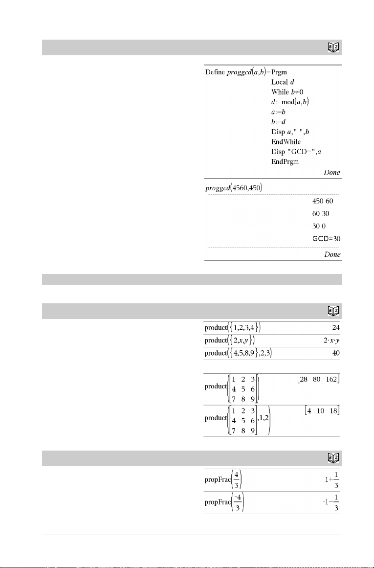
Prgm
Prgm
Block
EndPrgm
Template for creating a user-defined program. Must be used with the
Define, Define LibPub, or Define LibPriv command.
Block can be a single statement, a series of statements separated
with the “:” character, or a series of statements on separate lines.
Note for entering the example: In the Calculator application
on the handheld, you can enter multi-line definitions by pressing
@ instead of · at the end of each line. On the computer
keyboard, hold down Alt and press Enter.
Calculate GCD and display intermediate results.
Catalog
>
Product (PI)
product()
product(List[, Start[, End]]) ⇒ expression
Returns the product of the elements contained in List. Start and End
are optional. They specify a range of elements.
product(Matrix1[, Start[, End]]) ⇒ matrix
Returns a row vector containing the products of the elements in the
columns of Matrix1. Start and end are optional. They specify a range
of rows.
propFrac()
propFrac(Expr1[, Va r ]) ⇒ expression
propFrac(rational_number) returns rational_number as the sum
of an integer and a fraction having the same sign and a greater
denominator magnitude than numerator magnitude.
See Π(), page 136.
Catalog
>
Catalog
>
TI-Nspire™ CAS Reference Guide 83
Page 90

propFrac()
propFrac(rational_expression,Var ) returns the sum of proper
ratios and a polynomial with respect to Va r . The degree of Va r in the
denominator exceeds the degree of Va r in the numerator in each
proper ratio. Similar powers of Va r are collected. The terms and their
factors are sorted with Var as the main variable.
If Var is omitted, a proper fraction expansion is done with respect to
the most main variable. The coefficients of the polynomial part are
then made proper with respect to their most main variable first and so
on.
For rational expressions, propFrac() is a faster but less extreme
alternative to expand().
You can use the propFrac() function to represent mixed fractions
and demonstrate addition and subtraction of mixed fractions.
Q
Catalog
>
QR
QR Matrix, qMatrix, rMatrix[, Tol ]
Calculates the Householder QR factorization of a real or complex
matrix. The resulting Q and R matrices are stored to the specified
Matrix. The Q matrix is unitary. The R matrix is upper triangular.
Optionally, any matrix element is treated as zero if its absolute value
is less than Tol . This tolerance is used only if the matrix has floatingpoint entries and does not contain any symbolic variables that have
not been assigned a value. Otherwise, To l is ignored.
• If you use
•If Tol is omitted or not used, the default tolerance is calculated
/
mode to Approximate, computations are done using floatingpoint arithmetic.
as:
5Eë14 ·max(dim(Matrix)) ·rowNorm(Matrix)
· or set the Auto or Approximate
Catalog
The floating-point number (9.) in m1 causes results to be
calculated in floating-point form.
>
84 TI-Nspire™ CAS Reference Guide
Page 91

QR
The QR factorization is computed numerically using Householder
transformations. The symbolic solution is computed using GramSchmidt. The columns in qMatName are the orthonormal basis
vectors that span the space defined by matrix.
Catalog
>
QuadReg
QuadReg X,Y [, Freq] [, Category, Include]]
Computes the quadratic polynomial regression y = a·x2+b·x+c on
lists X and Y with frequency Freq. A summary of results is stored in
the stat.results variable. (See page 105.)
All the lists must have equal dimension except for Include.
X and Y are lists of independent and dependent variables.
Freq is an optional list of frequency values. Each element in Freq
specifies the frequency of occurrence for each corresponding X and Y
data point. The default value is 1. All elements must be integers | 0.
Category is a list of numeric category codes for the corresponding X
and Y data.
Include is a list of one or more of the category codes. Only those data
items whose category code is included in this list are included in the
calculation.
Output variable Description
stat.RegEqn
stat.a, stat.b, stat.c Regression coefficients
2
stat.R
stat.Resid Residuals from the regression
stat.XReg List of data points in the modified X List actually used in the regression based on restrictions of Freq,
stat.YReg List of data points in the modified Y List actually used in the regression based on restrictions of Freq,
stat.FreqReg List of frequencies corresponding to stat.XReg and stat.YReg
Regression equation: a·x2+b·x+c
Coefficient of determination
Category List, and Include Categories
Category List, and Include Categories
Catalog
>
TI-Nspire™ CAS Reference Guide 85
Page 92

QuartReg
QuartReg X,Y [, Freq] [, Category, Include]]
Computes the quartic polynomial regression
4
y = a
·x
+b·x3+c· x2+d·x+e on lists X and Y with frequency
Freq. A summary of results is stored in the stat.results variable. (See
page 105.)
All the lists must have equal dimension except for Include.
X and Y are lists of independent and dependent variables.
Freq is an optional list of frequency values. Each element in Freq
specifies the frequency of occurrence for each corresponding X and Y
data point. The default value is 1. All elements must be integers
Category is a list of numeric category codes for the corresponding X
and Y data.
Include is a list of one or more of the category codes. Only those data
items whose category code is included in this list are included in the
calculation.
Output variable Description
stat.RegEqn
stat.a, stat.b, stat.c,
stat.d, stat.e
2
stat.R
stat.Resid Residuals from the regression
stat.XReg List of data points in the modified X List actually used in the regression based on restrictions of Freq,
stat.YReg List of data points in the modified Y List actually used in the regression based on restrictions of Freq,
stat.FreqReg List of frequencies corresponding to stat.XReg and stat.YReg
Regression equation: a·x4+b·x3+c· x2+d·x+e
Regression coefficients
Coefficient of determination
Category List, and Include Categories
Category List, and Include Categories
| 0.
Catalog
>
86 TI-Nspire™ CAS Reference Guide
Page 93
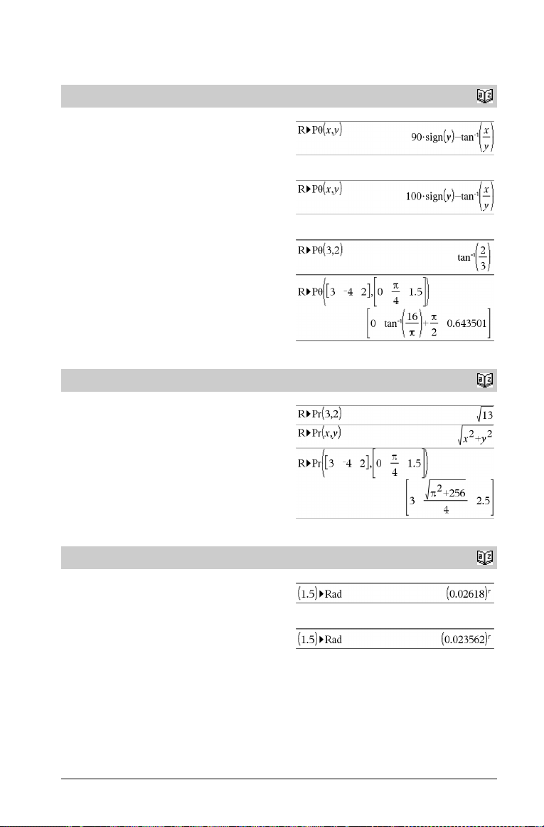
R
R4Pq()
R4Pq (xExpr, yExpr) ⇒ expression
R4Pq (xList, yList) ⇒ list
R4Pq (xMatrix, yMatrix) ⇒ matrix
Returns the equivalent q-coordinate of the
(x,y) pair arguments.
Note: The result is returned as a degree, gradian or radian angle,
according to the current angle mode setting.
R4Pr()
R4Pr (xExpr, yExpr) ⇒ expression
R4Pr (xList, yList) ⇒ list
R4Pr (xMatrix, yMatrix) ⇒ matrix
Returns the equivalent r-coordinate of the (x,y) pair arguments.
In Degree angle mode:
In Gradian angle mode:
In Radian angle mode:
In Radian angle mode:
Catalog
Catalog
>
>
4
Rad
Expr14Rad ⇒ expression
Converts the argument to radian angle measure.
In Degree angle mode:
In Gradian angle mode:
Catalog >
TI-Nspire™ CAS Reference Guide 87
Page 94

rand()
rand() ⇒ expression
rand(#Trials) ⇒ list
rand() returns a random value between 0 and 1.
rand(#Trials) returns a list containing #Trials random values
between 0 and 1.
Sets the random-number seed.
Catalog
>
randBin()
randBin(n, p) ⇒ expression
randBin(n, p, #Trials) ⇒ list
randBin(n, p) returns a random real number from a specified
Binomial distribution.
randBin(n, p, #Trials) returns a list containing #Trials random real
numbers from a specified Binomial distribution.
randInt()
randInt(lowBound,upBound) ⇒ expression
randInt(lowBound,upBound ,#Trials) ⇒ list
randInt(lowBound,upBound) returns a random integer within the
range specified by lowBound and upBound integer bounds.
randInt(lowBound,upBound ,#Trials) returns a list containing
#Trials random integers within the specified range.
randMat()
randMat(numRows, numColumns) ⇒ matrix
Returns a matrix of integers between -9 and 9 of the specified
dimension.
Both arguments must simplify to integers.
randNorm()
randNorm(m, s) ⇒ expression
randNorm(m, s, #Trials) ⇒ list
randNorm(m, s) returns a decimal number from the specified
normal distribution. It could be any real number but will be heavily
concentrated in the interval [mN3·s, m+3·s].
randNorm(m, s, #Trials) returns a list containing #Trials decimal
numbers from the specified normal distribution.
Catalog
>
Catalog
>
Catalog
>
Note: The value s in this matr ix will change each time you press
·.
Catalog
>
randPoly()
randPoly(Va r , Order) ⇒ expression
Returns a polynomial in Va r of the specified Order. The coefficients
are random integers in the range ë9 through 9. The leading
coefficient will not be zero.
Catalog
>
Order must be 0–99.
88 TI-Nspire™ CAS Reference Guide
Page 95

randSamp()
randSamp(List,#Trials[,noRepl]) ⇒ list
Returns a list containing a random sample of #Trials trials from List
with an option for sample replacement (noRepl=0), or no sample
replacement (noRepl=1). The default is with sample replacement.
Catalog
>
RandSeed
RandSeed Number
If Number = 0, sets the seeds to the factory defaults for the randomnumber generator. If Number ƒ 0, it is used to generate two seeds,
which are stored in system variables seed1 and seed2.
real()
real(Expr1) ⇒ expression
Returns the real part of the argument.
Note: All undefined variables are treated as real variables. See also
imag()
, page 51.
real(List1) ⇒ list
Returns the real parts of all elements.
real(Matrix1) ⇒ matrix
Returns the real parts of all elements.
4Rect
Vec t o r 4Rect
Displays Vec t o r in rectangular form [x, y, z]. The vector must be of
dimension 2 or 3 and can be a row or a column.
Note: 4Rect is a display-format instruction, not a conversion
function. You can use it only at the end of an entry line, and it does
not update ans.
Note: See also 4Polar, page 79.
Catalog
Catalog
Catalog
>
>
>
TI-Nspire™ CAS Reference Guide 89
Page 96

4
Rect
complexValue 4Rect
Displays complexValue in rectangular form a+bi. The complexValue
can have any complex form. However, an reiq entry causes an error in
Degree angle mode.
Note: You must use parentheses for an (rq) polar entry.
Catalog
>
In Radian angle mode:
In Gradian angle mode:
In Degree angle mode:
Note: To type , select it from the symbol list in the Catalog.
ref()
ref(Matrix1[, To l]) ⇒ matrix
Returns the row echelon form of Matrix1.
Optionally, any matrix element is treated as zero if its absolute value
is less than Tol . This tolerance is used only if the matrix has floatingpoint entries and does not contain any symbolic variables that have
not been assigned a value. Otherwise, To l is ignored.
• If you use
•If Tol is omitted or not used, the default tolerance is calculated
Note: See also rref(), page 93.
remain()
remain(Expr1, Expr2) ⇒ expression
remain(List1, List2) ⇒ list
remain(Matrix1, Matrix2) ⇒ matrix
Returns the remainder of the first argument with respect to the
second argument as defined by the identities:
remain(x,0) x
remain(x,y) xNy·iPart(x/y)
As a consequence, note that remain(Nx,y) Nremain(x,y). The
result is either zero or it has the same sign as the first argument.
Note: See also mod(), page 68.
/
mode to Approximate, computations are done using floatingpoint arithmetic.
as:
5Eë14 ·max(dim(Matrix1)) ·rowNorm(Matrix1)
· or set the Auto or Approximate
Catalog
Catalog
>
>
90 TI-Nspire™ CAS Reference Guide
Page 97

Return
Return [Expr]
Returns Expr as the result of the function. Use within a
Func...EndFunc block.
Note: Use Return without an argument within a
Prgm...EndPrgm block to exit a program.
Note for entering the example: In the Calculator application
on the handheld, you can enter multi-line definitions by pressing
@ instead of · at the end of each line. On the computer
keyboard, hold down Alt and press Enter.
Catalog
>
right()
right(List1[, Num]) ⇒ list
Returns the rightmost Num elements contained in List1.
If you omit Num, returns all of List1.
right(sourceString[, Num]) ⇒ string
Returns the rightmost Num characters contained in character string
sourceString.
If you omit Num, returns all of sourceString.
right(Comparison) ⇒ expression
Returns the right side of an equation or inequality.
root()
root(Expr) ⇒ root
root(Expr1, Expr2) ⇒ root
root(Expr) returns the square root of Expr.
root(Expr1, Expr2) returns the Expr2 root of Expr1. Expr1 can be
a real or complex floating point constant, an integer or complex
rational constant, or a general symbolic expression.
Note: See also Nth root template, page 1.
rotate()
rotate(Integer1[,#ofRotations]) ⇒ integer
Rotates the bits in a binary integer. You can enter Integer1 in any
number base; it is converted automatically to a signed, 64-bit binary
form. If the magnitude of Integer1 is too large for this form, a
symmetric modulo operation brings it within the range.
If #ofRotations is positive, the rotation is to the left. If #ofRotations
is negative, the rotation is to the right. The default is ë1 (rotate right
one bit).
For example, in a right rotation:
Catalog
>
Catalog
>
Catalog
>
In Bin base mode:
To see the entire result, press £ and then use ¡ and ¢ to
move the cursor.
In Hex base mode:
TI-Nspire™ CAS Reference Guide 91
Page 98

rotate()
Each bit rotates right.
0b00000000000001111010110000110101
Rightmost bit rotates to leftmost.
produces:
0b10000000000000111101011000011010
The result is displayed according to the Base mode.
rotate(List1[,#ofRotations]) ⇒ list
Returns a copy of List1 rotated right or left by #of Rotations
elements. Does not alter List1.
If #ofRotations is positive, the rotation is to the left. If #of Rotations
is negative, the rotation is to the right. The default is ë1 (rotate right
one element).
rotate(String1[,#ofRotations]) ⇒ string
Returns a copy of String1 rotated right or left by #ofRotations
characters. Does not alter String1.
If #ofRotations is positive, the rotation is to the left. If #ofRotations
is negative, the rotation is to the right. The default is ë1 (rotate right
one character).
Catalog
>
Important: To enter a binary or hexadecimal number, always
use the 0b or 0h prefix (zero, not the letter O).
In Dec base mode:
round()
round(Expr1[, digits]) ⇒ expression
Returns the argument rounded to the specified number of digits after
the decimal point.
digits must be an integer in the range 0–12. If digits is not included,
returns the argument rounded to 12 significant digits.
Note: Display digits mode may affect how this is displayed.
round(List1[, digits]) ⇒ list
Returns a list of the elements rounded to the specified number of
digits.
round(Matrix1[, digits]) ⇒ matrix
Returns a matrix of the elements rounded to the specified number of
digits.
rowAdd()
rowAdd(Matrix1, rIndex1, rIndex2) ⇒ matrix
Returns a copy of Matrix1 with row rIndex2 replaced by the sum of
rows rIndex1 and rIndex2.
rowDim()
rowDim(Matrix) ⇒ expression
Returns the number of rows in Matrix.
Note: See also colDim(), page 16.
Catalog
Catalog
Catalog
>
>
>
92 TI-Nspire™ CAS Reference Guide
Page 99

rowNorm()
rowNorm(Matrix) ⇒ expression
Returns the maximum of the sums of the absolute values of the
elements in the rows in Matrix.
Note: All matrix elements must simplify to numbers. See also
colNorm(), page 16.
Catalog
>
rowSwap()
rowSwap(Matrix1, rIndex1, rIndex2) ⇒ matrix
Returns Matrix1 with rows rIndex1 and rIndex2 exchanged.
rref()
rref(Matrix1[, To l]) ⇒ matrix
Returns the reduced row echelon form of Matrix1.
Optionally, any matrix element is treated as zero if its absolute value
is less than Tol . This tolerance is used only if the matrix has floatingpoint entries and does not contain any symbolic variables that have
not been assigned a value. Otherwise, To l is ignored.
• If you use
•If Tol is omitted or not used, the default tolerance is calculated
Note: See also ref(), page 90.
/
mode to Approximate, computations are done using floatingpoint arithmetic.
as:
5Eë14 ·max(dim(Matrix1)) ·rowNorm(Matrix1)
· or set the Auto or Approximate
Catalog
Catalog
>
>
S
sec()
sec(Expr1) ⇒ expression
sec(List1) ⇒ list
Returns the secant of Expr1 or returns a list containing the secants of
all elements in List1.
Note: The argument is interpreted as a degree, gradian or radian
angle, according to the current angle mode settin g. You can use ó,G,
orôto override the angle mode temporarily.
In Degree angle mode:
TI-Nspire™ CAS Reference Guide 93
Catalog
>
Page 100

sec/()
sec/(Expr1) ⇒ expression
sec/(List1) ⇒ list
Returns the angle whose secant is Expr1 or returns a list containing
the inverse secants of each element of List1.
Note: The result is returned as a degree, gradian or radian angle,
according to the current angle mode setting.
In Degree angle mode:
In Gradian angle mode:
In Radian angle mode:
Catalog
>
sech()
sech(Expr1) ⇒ expression
sech(List1) ⇒ list
Returns the hyperbolic secant of Expr1 or returns a list containing t he
hyperbolic secants of the List1 elements.
sechê()
sechê(Expr1) ⇒ expression
sechê (List1) ⇒ list
Returns the inverse hyperbolic secant of Expr1 or returns a list
containing the inverse hyperbolic secants of each element of List1.
seq()
seq(Expr, Va r, Low, High[, St ep]) ⇒ list
Increments Va r from Low through High by an increment of Step ,
evaluates Expr, and returns the results as a list. The original contents
of Var are still there after seq() is completed.
Var cannot be a system variable.
The default value for Ste p = 1.
Catalog
Catalog
In Radian angle and Rectangular complex mode:
Catalog
Press Ctrl+Enter /· to evaluate:
>
>
>
94 TI-Nspire™ CAS Reference Guide
 Loading...