

™
Introduction to
by Bernhard Kutzler
& Vlasta Kokol-Voljc
TI EXPLORATIONS™SOFTWARE

Bernhard KUTZLER
Vlasta KOKOL-VOLJC
Introduction to
TM
D
The following Derive™ 5 documentation is being
provided as a courtesy of the authors, Bernhard
Kutzler / Vlasta Kokol and the publisher Texas
Instruments. We invite you to use the following
abbreviated document during your personal
evaluation of Derive™ 5. Use of the document for
any other purpose is strictly prohibited.
A book for learning how to use D
ERIVE
5
ERIVE
5

Kutzler, Bernhard & Kokol-Voljc, Vlasta
Introduction to D
ERIVE
5
2000
2000 Kutzler & Kokol-Voljc OEG, Austria
1. Edition, 1. Printing: March 2000
Typesetting: Bernhard Kutzler, Leonding, Austria
Cover art: Texas Instruments Incorporated, Dallas, Texas, USA
The author and publisher make no warranty of any kind, expressed or implied, with regard to the
documentation contained in this book. The author and publisher shall not be liable in any event for
incidental or consequental damages in connection with, or arising out of, the furnishing, performance
or use of this text.
No part of this publication may be reproduced, stored in a retrieval system, or transmitted, in any
form, or by any means, electronic, mechanical, photocopying, recording or otherwise, without prior
permission, in writing, from the publisher.
ERIVE
is a trademark of Texas Instruments Incorporated
D
INDOWS
W
, W
INDOWS
95, W
INDOWS
NT, and WIN32S are registered trademarks of Microsoft Corp.

Table of Contents
Introduction ............................................................................................................................................. 1
Chapter 1: First Steps ............................................................................................................................. 3
Chapter 2: Documenting Polynomial Zero Finding ........................................................................... 23
Chapter 3: The Whole and Its Parts – Subexpressions ..................................................................... 43
Chapter 4: Equations and Inequalities ................................................................................................ 63
Chapter 5: Approximate Versus Exact Computations ...................................................................... 83
Chapter 6: Sequences and Families of Curves ................................................................................... 95
Chapter 7: Investigations in Space .................................................................................................... 117
Chapter 8: What Is ‘Simple’? .............................................................................................................. 135
Chapter 9: Vectors, Matrices, and Sets ............................................................................................. 153
Chapter 10: Parametric Plots ............................................................................................................. 171
Chapter 11: Towards a Module for Analytical Geometry ............................................................... 185
Chapter 12: Some Calculus ................................................................................................................ 203
Chapter 13: More on Plotting ............................................................................................................. 221
ERIVE
Chapter 14: What Else Can D
ERIVE
Learn More about D
Appendix A: D
Appendix B: Factory Default D
Index ..................................................................................................................................................... 269
ERIVE
................................................................................................................... 261
Startup Options ................................................................................................ 263
Do? ............................................................................................ 243
ERIVE
................................................................................................ 265
iii

Preface
v
The desire to make D
Many thanks to Albert Rich and Theresa Shelby, the principal authors of D
continuous support during the writing of this book.
Many thanks to Patricia Littlefield and David Stoutemyer who polished the language of this
book.
Bernhard Kutzler & Vlasta Kokol-Voljc, February 2000
ERIVE
5 easily and quickly accessible led to this book.
ERIVE
5, for their

Introduction
ERIVE
D
is a mathematical computer program. It processes algebraic variables, expressions,
equations, functions, vectors, and matrices like a scientific calculator processes floating point
numbers. D
calculus, and plot graphs in 2 and 3 dimensions. The main strength of D
algebra and powerful graphics. It is an excellent tool for doing and applying mathematics, for
documenting mathematical work, and for teaching and learning mathematics.
For a teacher and student, D
mathematics. By providing numeric, algebraic, and graphic capabilities together with seamless
integration of these, D
mathematics. You will find that many topics can be treated more efficiently and effectively than
by using traditional methods. Many problems that require extensive and laborious training at
school can be solved with a single keystroke using D
performing long mathematical calculations. While D
mechanical/algorithmic parts of solving a problem, students can concentrate on the
mathematical meaning of concepts. Instead of teaching and learning boring technical skills,
teachers and students can concentrate on the exciting and useful techniques of problem solving.
It has proven to be highly supportive for the cognitive development of advanced mathematical
concepts.
For an engineer, D
operations and functions and for visualizing problems and their solutions in various ways. If you
use D
knowledgeable mathematical assistant that is easy to use.
ERIVE
can perform numeric and symbolic computations, algebra, trigonometry,
ERIVE
are symbolic
ERIVE
is the ideal tool for supporting the teaching and the learning of
ERIVE
enables new approaches in teaching, learning, and understanding
ERIVE
: It eliminates the drudgery of
ERIVE
takes the burden of doing the
ERIVE
is the ideal tool for fast and effective access to numerous mathematical
ERIVE
for your everyday mathematical work, you will find it a tireless, powerful, and
This book is for learning how to use D
ERIVE
5 by private study. Install D
ERIVE
5 on your
computer. Starting with the first chapter, you will learn step by step how to use the program.
Follow all instructions and examples. The text leads you through several mathematical topics
that are used for learning how to solve mathematical problems with D
ERIVE
examples also provide ideas for using D
during teaching; some of them are explained in
ERIVE
. Many of the
more detail in “Educator’s footnotes.” Paragraphs starting with the symbol give instructions
about what you should do on your computer. Hundreds of screen dumps ensure that you will not
get lost on this journey.

2 Introduction
By solving typical mathematical high school level problems, you will learn to handle D
ERIVE
5 as
much as necessary for everyday use and for teaching or learning mathematics. You will learn
how to use the major commands, keys, and functions. At the end of each chapter you will find a
summary of the features learned in that chapter. The Quick Reference Guide at the end of the
book is a summary of commands, keys, functions, and utility files, which is organized by tasks.
The index at the end is useful if you need to locate a particular portion of the text.
All you need to run D
INDOWS
W
NT.
ERIVE
5 is a PC compatible computer with W
It is assumed that you know how to use computers and the W
screen shots in this book were produced from D
D
ERIVE
on W
INDOWS
95 or 98, some of the screens may appear slightly different.
ERIVE
running on W
This book introduces all features and functions that are required for routine use of D
There is more functionality than can be described here. This book is
ERIVE
. A complete reference to all features is included with the software as online help. Some
D
INDOWS
95, W
INDOWS
operating system. The
INDOWS
not
a reference manual for
INDOWS
98, or
NT. If you are running
ERIVE
5.
of the chapters give examples of how to use the online help.
ERIVE
We plan to write additional texts on D
http://series.bk-teachware.com
for new texts and local dealer information.
5. Please regularly look at the web site
Have fun reading and discovering.
Chapter 1: First Steps
ERIVE
D
makes it easy to perform mathematical operations: Enter an expression, apply a
command, and a new expression is obtained. All expressions can be used for new
computations—just like on a piece of paper. This chapter teaches the basic techniques of using
ERIVE
D
5. Note: For simplicity, we will abbreviate D
This text assumes that you use a factory default D
match those in this book. If you just installed D
version of D
ERIVE
that was used by someone else, we recommend that you turn it into a factory
default version now. Appendix B gives instructions on how to do this.
ERIVE
Start D
by double clicking on the D
desktop, you probably will find D
ERIVE
ERIVE
on the
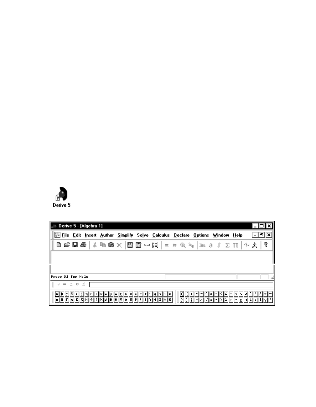
The following screen appears after a few seconds:
ERIVE
ERIVE
. Only then will your screen images fully
ERIVE
, it is a factory default version. If you use a
icon. If there is no D
Start
menu or via
5 as D
ERIVE
throughout this text.
ERIVE
icon on your computer’s
Start>Programs
.
ERIVE
The D
•
•
•
•
•
•
•
screen comprises (from top to bottom):
the Titlebar
the Menu Bar
the Command Toolbar
a (currently empty) Algebra Window, also called the View
the Status Bar
the Expression Entry Toolbar, also called the entry line
the Greek Symbol Toolbar and the Math Symbol Toolbar
4 Chapter 1: First Steps
Work with D
After starting D
ERIVE
by entering expressions and applying commands, thus creating a worksheet.
ERIVE
, the system is ready to accept user input via the Expression Entry Toolbar,
as is indicated by the blinking cursor in the toolbar’s entry field. Input mode can be implemented
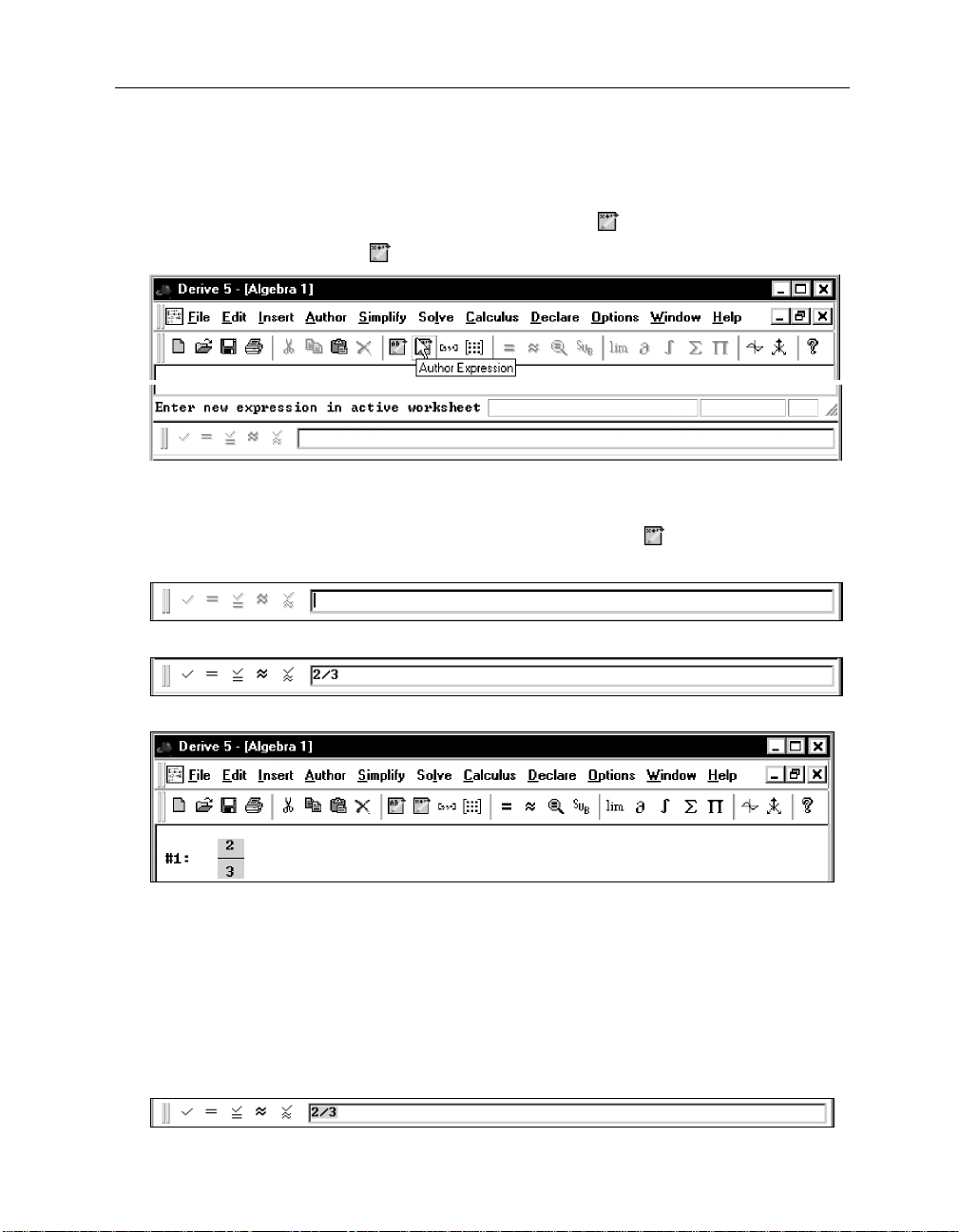
with the Command Toolbar’s tenth button from the left, labeled
Learn more about the button
The message
Author Expression
Enter new expression in active work sheet
Prepare for entering an expression: Move the mouse pointer onto
by moving the mouse pointer onto it.
below the cursor is the button’s title. The Status Bar message
is the button’s function description.
.
, then click (i.e. press
and release) the left mouse button.
Enter the fraction:
2/3
End the input with the ‘Enter’-key
ERIVE
D
displays this expression as a fraction with a horizontal line, a numerator, and a
(¢)
.
denominator, i.e. in “2-dimensional” output format, as opposed to the “1-dimensional” or “linear”
input format used for entering the number. The expression’s unique label number, #1, is shown
ERIVE
to the left of the expression. D
focus
) is still in the entry line. Also observe that a copy of the input is still in the entry field and is
is again ready to accept the next input, i.e. input control (the
entirely highlighted. This has the same meaning as in text editors and word processors. You can
remove the highlighting with the right arrow key, then edit the string of symbols, or you can
replace the marked string by typing new symbols.
Kutzler & Kokol-Voljc: Introduction to D
11
(¢)
+
23
.
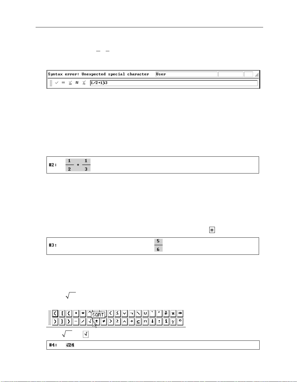
Replace the last input by
Enter
1/2+1&3
55
ERIVE
with an intentional typographical error:
When a syntax error is detected, the cursor is moved to the location of the error and the cause of
the error is displayed in the Status Bar’s first pane. In the above example D
ERIVE
discovered an
unexpected special character. In some cases (for example, when entering an opening
parenthesis instead of the division symbol) there are several errors possible, and D
ERIVE
can only
guess.
Update the input to
the backspace key
Conclude with
(¢)
1/2+1/3
(æ_)
: Use the
) to delete the incorrect character, then type the division operator.
(Del)
key (or the right arrow key
.
(Æ)
followed by
The expression and its label, #2, are displayed. The new expression is highlighted in reverse
video. Expression #1 is no longer highlighted.
If you mistyped the input and want to delete the highlighted expression for a retry, use
move the focus into the algebra window, use the ‘Delete’ key
expression, then use the
Author Expression
button to move the focus back into the entry line.
(Del)
to delete the highlighted
(Esc)
to
An alternative technique for replacing an expression will be explained in Chapter 2.
Simplify expression #2 using the Command Toolbar’s
Simplify
button .
The result becomes the next expression with the label #3. By default, simplified expressions are
displayed centered. This makes it easy to distinguish between entry and result. As with many
ERIVE
other behaviors of D
Even after using the
24
expression,
. To enter the square root symbol, use the respective button on the Math
, this can be customized if desired.
Simplify
button, the focus still is in the entry line. Enter the next
Symbol Toolbar:
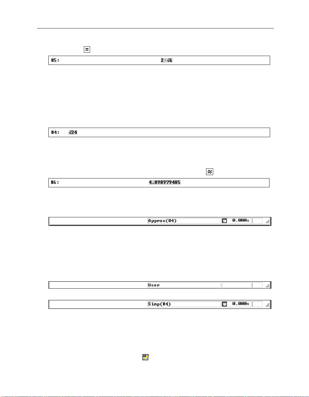
Enter
24
as: 24
(¢)
6 Chapter 1: First Steps
Simplify using
.
This is different from what an “ordinary” calculator would produce. A mathematician once
“How do you recognize a mathematician?”
asked:
mathematician considers expression #5 a beautiful result.”
and suggested the following answer:
Most students strive to replace
such an expression by the corresponding floating point approximation. D
ERIVE
can do this as
“A
well: Highlight expression #4 so that you can apply a different command to it.
Highlight expression #4 by moving the mouse pointer anywhere in the row occupied by the
expression, then clicking the left mouse button.
Selecting an expression with the mouse button is one technique of highlighting it. An alternative
technique is first to move the focus into the algebra window (if necessary) using the
then using the cursor keys
(½)
or
(¼)
to move the highlighting one expression up or down.
(Esc)
key,
Approximate using the Command Toolbar’s
Approximate
button .
While an expression is highlighted, the Status Bar’s second pane shows the automatically
generated expression annotation. The third pane shows the computing time in case the expres-
sion was obtained as a result of a computation. For expression #6 this is:
The automatically generated annotation explains how the expression was obtained.
Approx(#4)
means that the expression was obtained by applying the
command) to expression #4. The computation time displayed in the third pane,
Approximate
0.000s
button (or
,
indicates that the calculation took less than 0.001 seconds (the time may be different on your
computer).
Highlight expression #4, . . .
. . . then expression #5.,
The annotation of expression #4,
expression #5,
Simp(#4)
User
, means that it was entered by the user; the annotation of
, indicates that the expression was obtained by applying the
Simplify
button (or command) to expression #4. The first pane is always available for messages
associated with a menu item, button, or command status.
ERIVE
worksheets also can include text and other objects. The easiest way of entering text is via
D
the Command Toolbar’s
Insert Text
button . New expressions are added at the end of the
Kutzler & Kokol-Voljc: Introduction to D
57
ERIVE
worksheet. Other objects (including text objects) are added after the highlighted object. To
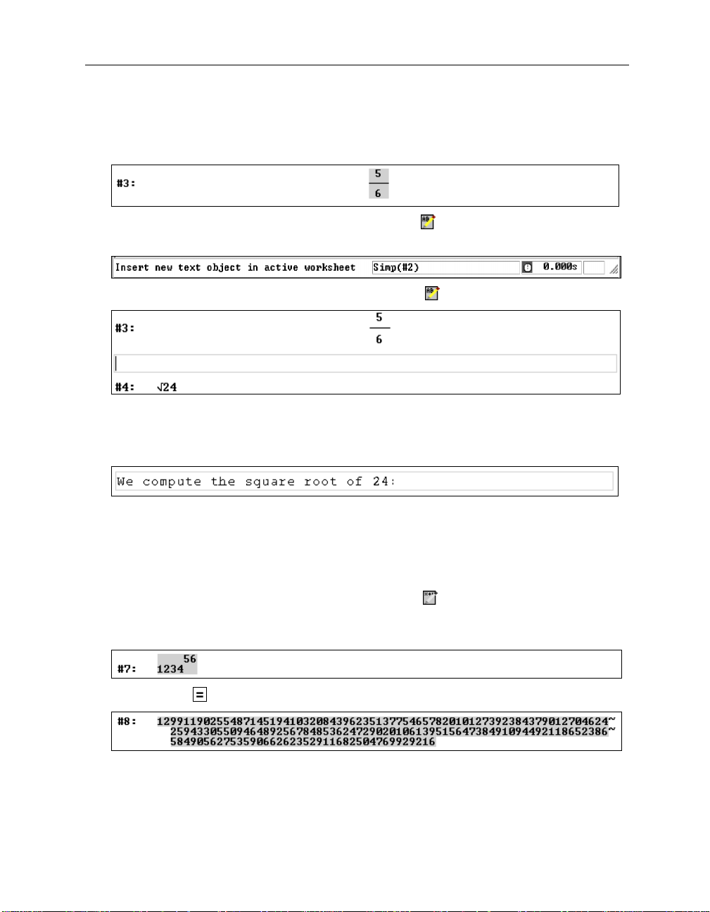
insert a text object above the square root of 24, first highlight the object that is now above it.
Highlight expression #3.
Display a function description of the
Insert Text
button by moving the mouse pointer
onto it.
Insert a text object by clicking on the
Insert Text
button .
Highlighting of a text object is indicated by a frame around it. The blinking cursor inside
indicates text editing mode.
Enter the text:
We compute the square root of 24:
A text object allows simple text editing similar to what you can do in standard text editors. Later
you will learn how to change the font size, alignment, color, etc.
As a next example compute
56
. Due to the previous activity, the focus now is in the algebra
1234
window. Before you can enter another expression, move the focus into the entry line.
1234^56
Enter
by using the
of digits followed by
Author Expression
(¢)
. The exponentiation operator ^ can be found on both the
button , then typing the respective string
keyboard and the Math Symbol Toolbar. (It is the sixth symbol from the left in the first row.)
Simplify using
.
This is a very big number. For those who want to know the number of digits, there are two
methods to find out: First, you can count them. Second, you can approximate the number.
8 Chapter 1: First Steps
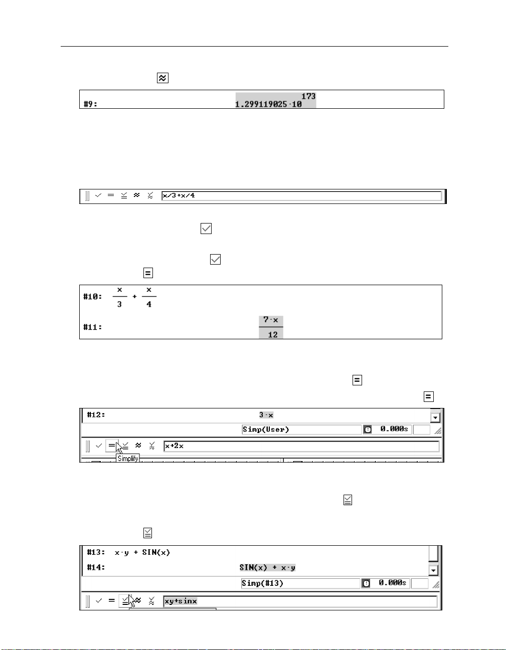
Approximate using
.
The answer is displayed in scientific notation. Since the count of whole digits is one more than
the power of 10, the number has 173+1 = 174 digits.
In the next exercise, you will learn a different technique of entering expressions by using the
buttons preceding the entry field.
Type into the entry line
x/3+x/4
this time
without concluding with
(¢)
.
Note the five buttons left of the entry field. The usual technique of moving the mouse pointer
onto a button reveals the first one,
, as the
has the same effect as concluding the input with the
Enter the above expression with
Simplify
Unlike ordinary calculators, D
button .
ERIVE
can perform nonnumeric (symbolic, algebraic) computations
Author Expression
(¢)
button. Selecting this button
key. Try it:
, then simplify as usual using the Command Toolbar’s
such as simplifying expression #10 into expression #11.
For the next example use the Expression Entry Toolbar’s second button,
To simplify
+
2xx
immediately, type
x+2x
then select the entry line’s
.
Simplify
button .
This button simplified the entered expression immediately without the usual display of the
unsimplified expression. Note the result’s annotation:
For the next example use the Expression Entry Toolbar’s third button,
Enter and simplify
Simplify
button .
+
sinxy x
by typing
xy+sinx
Simp(User)
.
then using the entry line’s
Author and

Kutzler & Kokol-Voljc: Introduction to D
59
ERIVE
This button produced two expressions, #13 and #14 and has the same effect as entering the
unsimplified expression with
(¢)
or
, then simplifying it with . It is, therefore, a convenient
shortcut for the frequently used “enter and simplify.” This example also shows how convenient
fast input is in D
ERIVE
. You can enter expressions just as you would write them on paper. For ‘
x
times y ‘ simply enter xy. No multiplication operator is needed between x and y. For ‘Sine of x ‘
simply enter sinx. No parentheses are needed around x.
The Expression Entry Toolbar has buttons for entering, simplifying, entering & simplifying,
approximating, and entering & approximating expressions.
The simplified expression #14 differs from the unsimplified expression #13 only in the order in
which its terms are displayed. While unsimplified expressions are displayed as they were entered
(except for the 2-dimensional pretty print format), simplified expressions are displayed in a
standardized format using a certain term ordering.
Back to how simple it is to enter expressions. A consequence of the convenient fast input, such
xy+sinx
as
for
⋅+
sin( )xy x
, is that variable names can consist of only one character (for
example x and y). This suffices most of the time, but if you need to use multicharacter variable
names, D
ERIVE
allows this, too (for example
time
or x12). Using multicharacter variable names
will be explained in Chapter 14.
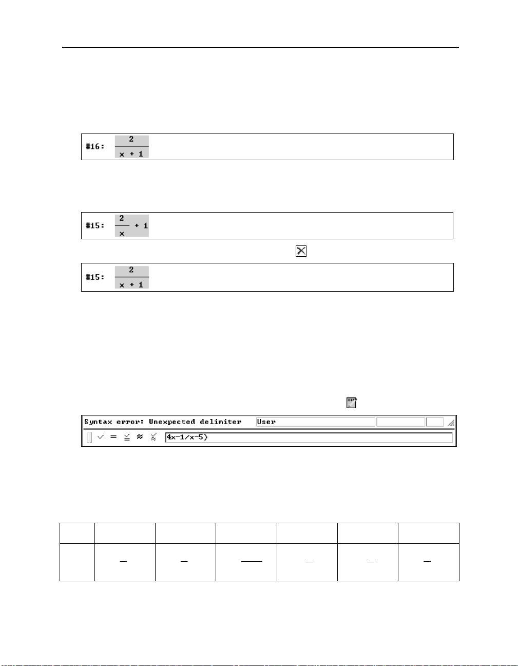
Clearly, you cannot omit all parentheses. For example, you will need to parenthesize the
denominator to enter a rational expression such as
2
. If the parentheses are omitted in this
+
1x
example, the resulting expression has a different meaning.
Enter:
2/x+1
Oops—the expression on the screen looks different from the intended expression! D
ERIVE
applies operations in the conventional order, for example multiplication and division before
addition and subtraction. As you can see from the above example, the 2-dimensional screen
display of an input provides you with valuable feedback about the soundness of your input.
1
Educator’s footnote:
the students to input expressions given to them on the chalkboard or a piece of paper. Because D
features 2-dimensional output of expressions, the students get an immediate feedback. If the
expression on the screen looks different from the one on the chalkboard or paper, then the input was
wrong, and they must try again. When the teacher lets students input expressions of increasing
complexity, they learn how to “linearize” expressions by trying and experimenting (trial and error),
and learn to understand the structure of expressions. In this way, they improve their competence in
recognizing structures, which is one of the basic mathematical skills important in many areas.
A very simple educational exercise with D
ERIVE
, therefore, consists of asking
1
ERIVE
10 Chapter 1: First Steps
When correcting the most recent input, you can take advantage of the fact that a copy of the
most recent input and the focus are still in the entry line.
To edit the expression use the right arrow key
input to
Now it looks correct. Since you don’t need expression #15 any more, delete it.
Prepare for deletion: Highlight expression #15 either with the mouse or with the keyboard’s
arrow keys after moving the focus into the algebra window using
2/(x+1)
by adding the parentheses, then enter the expression with
(Æ)
to remove the highlighting. Change the
(¢)
(Esc)
.
.
Delete expression #15: Use the
The expression that was expression #15 disappeared. The expression that was expression #16
has become expression #15. By default, automatic renumbering adjusts expression numbers so
that they begin with #1 and have no gaps.
Errors such as omitting a whole pair of parentheses may change the meaning of an expression,
as was the case in the previous example. If only one parenthesis is omitted, the input becomes a
meaningless character string, and D
syntax error message:
ERIVE
D
parenthesis can be spotted while a missing opening parenthesis obviously cannot, the first
alternative is used for the error message. Depending on how the expression should look, you
have to either delete the closing parenthesis or insert an opening parenthesis somewhere before
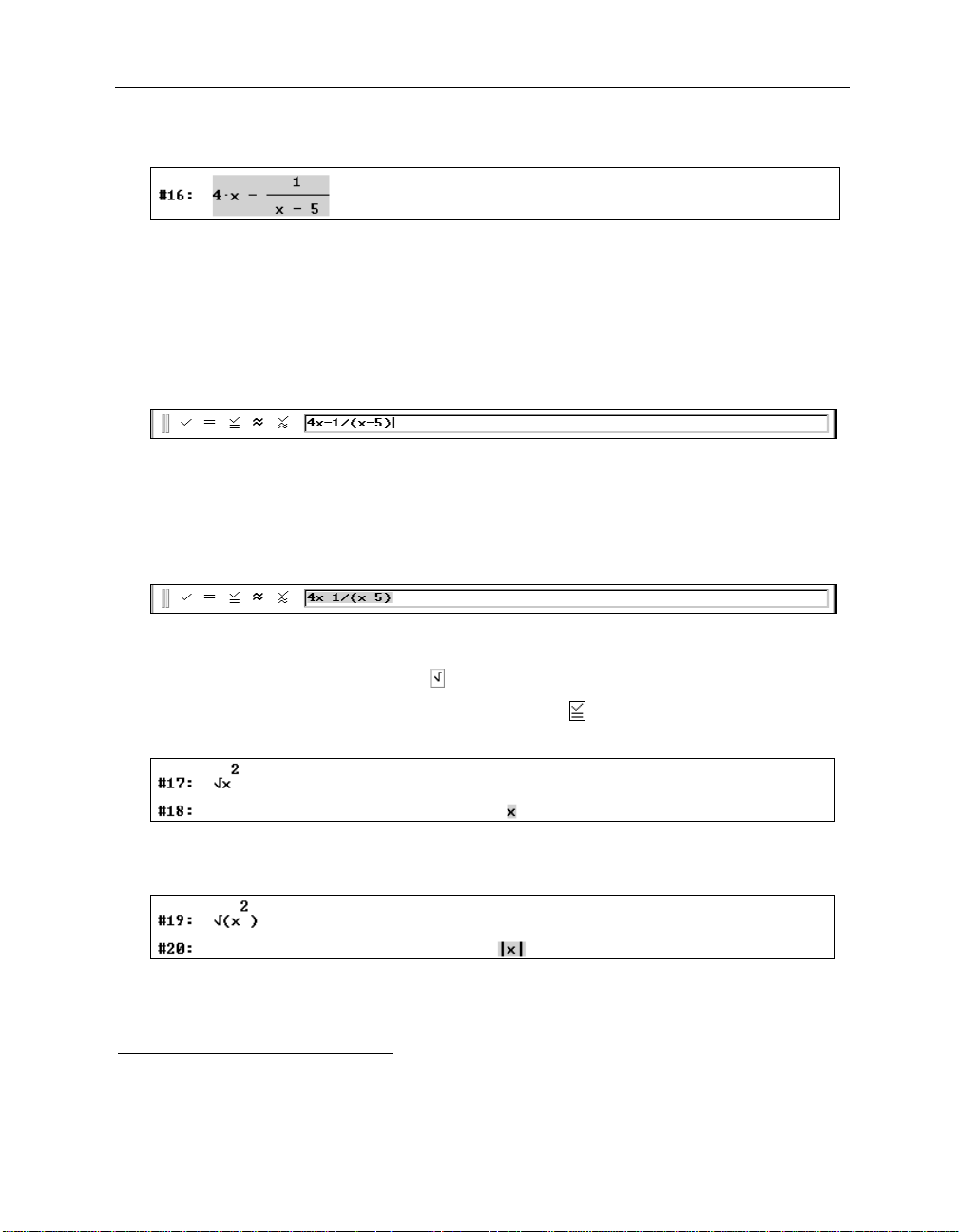
it. For the above example there are six possible repairs:
input
4x-1/x-5)
Enter
attempts to position the cursor in front of the expected error. Since a superfluous closing
4x-1/x-5 4x-1/x-(5) 4x-1/(x-5) 4x-(1/x-5) 4(x-1/x-5) (4x-1/x-5)
after moving the focus into the entry line with
Delete Object
ERIVE
will issue a warning in the form of an appropriate
button or press the
(Del)
.
key.
output
To choose the third variant insert an opening parenthesis between the division operator and the
variable x.
−−
45x
1
x
−−
45x
1
x
45x
1
−
−
x
45x
−−
1
x
1
−−
45x
x
45x
1
−−
x
Kutzler & Kokol-Voljc: Introduction to D
Edit the input string to
4x-1/(x-5)
511
ERIVE
2
then press
(¢)
.
When working with D
When focus is in the entry line,
Author Expression
the
ERIVE
, focus can be either in the entry line or in the algebra window (View).
(Esc)
will move focus into the View. When focus is in the View,
button or its hot key equivalent,
(F2)
, moves it into the entry line.
Another method to move focus is using the mouse. Focus is where one last moved the mouse
pointer to and then pressed the left mouse button.
Ensure that focus is in the entry line by moving the mouse pointer into the entry line’s entry
field, then clicking with the left mouse button.
The disadvantage of this method is that it removes highlighting if there was any, so now you
cannot simply replace the old input with a new one by starting to type the new input string. You
could use the backspace key several times to delete the old string, but a more elegant way is to
use the tab key.
Highlight the contents of the entry line with the tab key
x^2
Enter and simplify
button or to use the entry line’s
obtained from the Math Symbol Toolbar (
Type
√
x^2
√
. It is up to you to either use the ‘Enter’ key followed by the
then press
Enter and Simplify
(Ctrl)+(¢)
) or entered as
. This is the same as
button. The square root symbol √ can be
(ÿ)
.
(Ctrl)-(Q)
.
, i.e. this is a simple way to
Simplify
perform an “enter and simplify” operation without using the mouse.
As an alternative, introduce a pair of parentheses around
Enter and simplify:
2
Educator’s footnote:
students how many different expressions they can generate by inserting 1, 2 (or more) pairs of parentheses into a valid string of characters. This is another excellent exercise to help students gain an
understanding of the structure of expressions.
(x^2)
√
This is another example for an elementary educational use of D
x^2
.
ERIVE
. Ask
12 Chapter 1: First Steps
The last two examples are remarkable for two reasons. First, they demonstrate the importance
of using parentheses to differentiate between
2
x
). Second, expression #20 shows how carefully D
()
α
The third power of
−
is entered as follows:
1
2
x
(meaning
ERIVE
2
x
) and
()
simplifies expressions.
2
x
(meaning
This did not change anything. Now you have an opportunity to apply one of those commands for
which there is no equivalent Command Toolbar button.
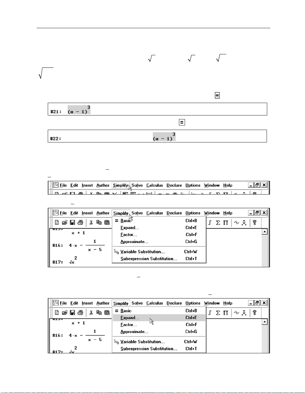
(α-1)^3
Enter
Try to expand expression #21, first by simplifying with
Prepare for opening the
Simplify
Open the
. (Insert Alpha with the Greek Symbol Toolbar button
command.
Simplify
Simplify
menu by clicking the left mouse button.
menu by moving the mouse pointer above the Menu Bar’s
.)
.
This menu offers several commands. The
expression.
Select this command by moving the mouse pointer above the word
Expand
command is appropriate for expanding an
Expand
. . .
Kutzler & Kokol-Voljc: Introduction to D
. . . then invoke the command by clicking on it with the left mouse button.
513
ERIVE
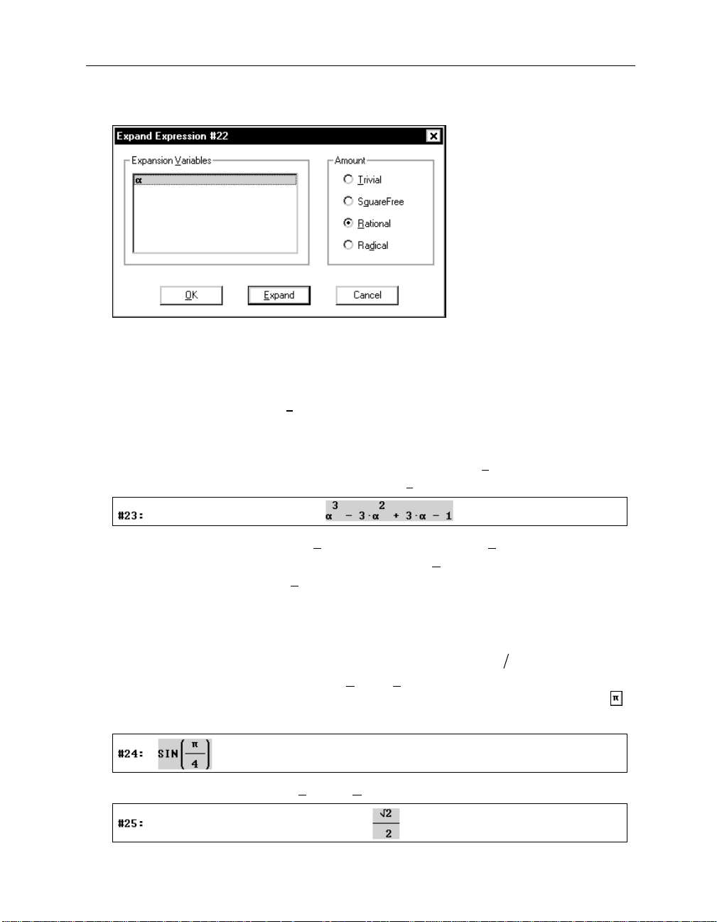
D
ERIVE
opens the
Expand Expression
dialog box. You will obtain similar dialog boxes with all
commands that require specification of parameters. The above dialog box requires the
specification of the expansion variable and the amount of expansion. Often it is enough to accept
the default specifications and immediately exit the dialog box with the ‘Enter’ key or by clicking
xpand_)
the default button, which here is
displayed.) Use the
(_Cancel_)
(_E
button or the
you want an unsimplified application of the
Perform the expansion with the suggested parameters by using
(¢)
because this is the default button or click on
A keyboard alternative for selecting the
following standard W
the underscore under the letter S in
underscore, but now without the
INDOWS
technique:
Simplify
(Alt)
. (The default button is the one prominently
(Esc)
EXPAND
Expansion
(Alt)+(S)
), then press
key to cancel the command. Use
function.
(_E
xpand_)
(_E
xpand_)
command from the
opens the
(E)
.)
Simplify
Simplify
menu (use
(again the letter with the
(_OK_)
(either press
menu is the
(S)
because of
, which is used only to open menus.) This technique
if
works for all menu commands.
For all buttons from the Command Toolbar there exist corresponding menu commands. Use
π
commands for the next example. Enter, simplify, then approximate
To enter the above expression, select the
sin(¹/4)
(¢)
. (Obtain π from either the Greek or the Math Symbol Toolbar. A button
Author>Expression
sin 4
command, then type
.
()
for this frequently used character is in both of these toolbars.)
Simplify expression #24 with the
Simplify>Basic
command.
14 Chapter 1: First Steps
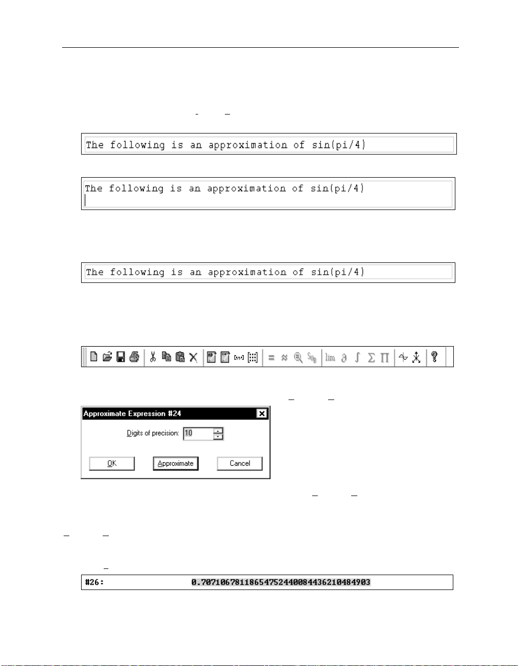
This is another “beautiful” result. Before computing an approximation, add an appropriate
comment to the worksheet in form of a text object.
Insert a text object with the
Insert>Text Object
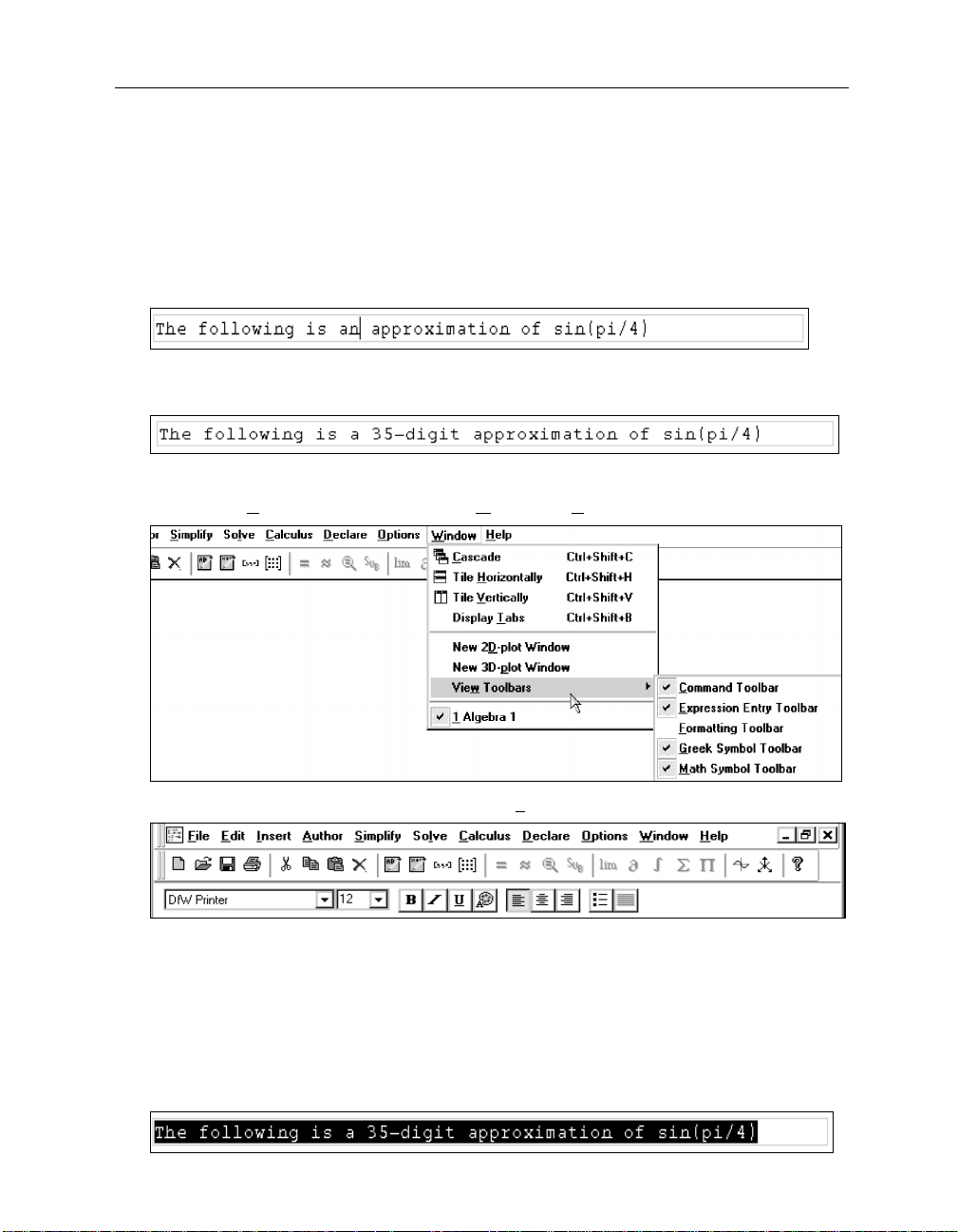
command, then type:
The following is an approximation of sin(pi/4)
(Try to) conclude the input with
(¢)
.
The ‘Enter’ key, used from within text editing mode, added an extra line to the text object. This
is not what was intended.
Delete the extra line using the backspace key
Note that while D
ERIVE
is in text editing mode, you have no access to certain buttons and menu
(æ_)
.
commands as you can see in the Command Toolbar. The inaccessible buttons and menu
commands appear dimmed. For example, the
Approximate
button is not available in text editing
mode now, because a text object is highlighted.
You need to highlight an expression before you can approximate it.
Highlight expression #24, then approximate it with
Simplify>Approximate
.
Other than the Command Toolbar’s
Approximate
button, the
Simplify>Approximate
command
invokes a dialog box in which you are asked to specify the number of digits of precision. The
currently displayed default value of 10 digits is also used by the
Simplify>Approximate
command allows you to temporarily change the default value for the next
Approximate
button. The
computation. Change the number to 35, then use the default dialog exit.
(_A
35
pproximate_)
Kutzler & Kokol-Voljc: Introduction to D
ERIVE
In D
you can specify virtually any precision, meaning number of significant digits used for
515
ERIVE
arithmetic. The practical limitations are given by the available memory and your patience. Note
that computing time increases with increasing precision.
Update your text to indicate the chosen precision.
Bring the text object into editing mode by clicking into it. Position the cursor immediately
after the word:
an
Change the text appropriately by using the backspace key
adding:
35-digit
(æ_)
Reducing the text’s font size requires the Formatting Toolbar to be on.
Open the
Turn the Formatting Toolbar on by selecting the
View Toolbars
submenu with the
Window>View Toolbars
Formatting Toolbar
to delete the letter n, then
command.
command.
For editing D
ERIVE
text, use the same techniques as in standard word processing programs. This
toolbar indicates that the font size is 12 points. Before you can reduce the font size to 10 points,
you need to highlight the respective portion of text.
Highlight the entire sentence. Either use the technique of dragging the mouse pointer (hold
the left mouse button down) from one end of the text to the other, or put the cursor at the
text’s end (or beginning), then repeatedly use the left (or right) arrow key together with the
shift key, or place the cursor anywhere in the text, then triple-click.
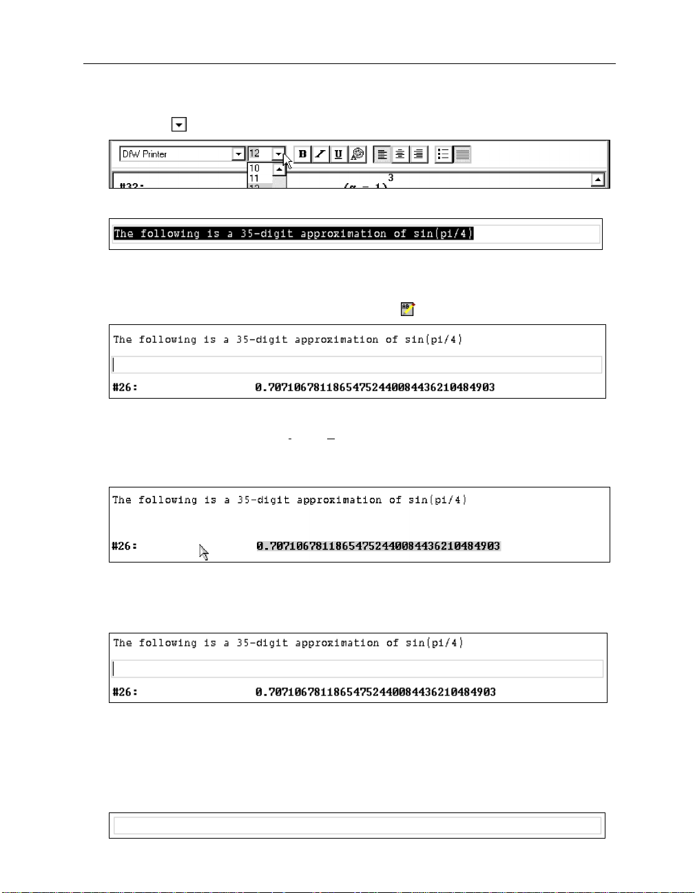
16 Chapter 1: First Steps
Prepare for changing the font size: Open the
clicking on
Select the number 10.
Alternatively, you could make the
.
Font Size
Font Size
field’s dropdown selection menu by
field active, then overwrite 12 with 10.
Now, announce the next example with an appropriate text.
Prepare for entering text using the
Insert Text
button .
Oops—this is the wrong position. The new text should appear at the end of the document. Since
Insert Text
the
button (as well as the
Insert>Text Object
command) adds the text object after the
highlighted object, you need to highlight expression #26 first.
Select expression #26.
Although the frame around the unintentionally inserted, empty text object disappeared, it is still
there. It can be deleted like any other object only after it is highlighted.
Highlight the text object by clicking into it.
Try to delete it, using the
(Del)
key.
This has no effect. Remember: Clicking inside a text object starts text editing mode. To select a
text object for deletion, copying, or moving, click (precisely) onto the frame or into the narrow
space left (or right) of the text object, or press
Select the text object for deletion using
(Esc)
(Esc)
from within text editing.
.
Kutzler & Kokol-Voljc: Introduction to D
517
ERIVE
The text object is selected now as is indicated by the frame around it. Make sure there is no
cursor inside it. If there is, press
Delete the empty text object using the
(Esc)
again.
(Del)
key.
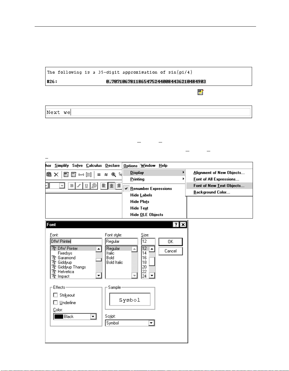
Insert a new text object after the highlighted expression #26 (using
the text “
Next we
.”
Note that this text again has font size 12 as you can see in the Formatting Toolbar’s
), then start entering
Font Size
field. Earlier you only changed the format of existing text. Changing the default format of all new
text objects is done via a command from the
To change the default setting of future text objects, select the
Text Objects
command.
Options>Display
menu.
Options>Display>Font of New
18 Chapter 1: First Steps
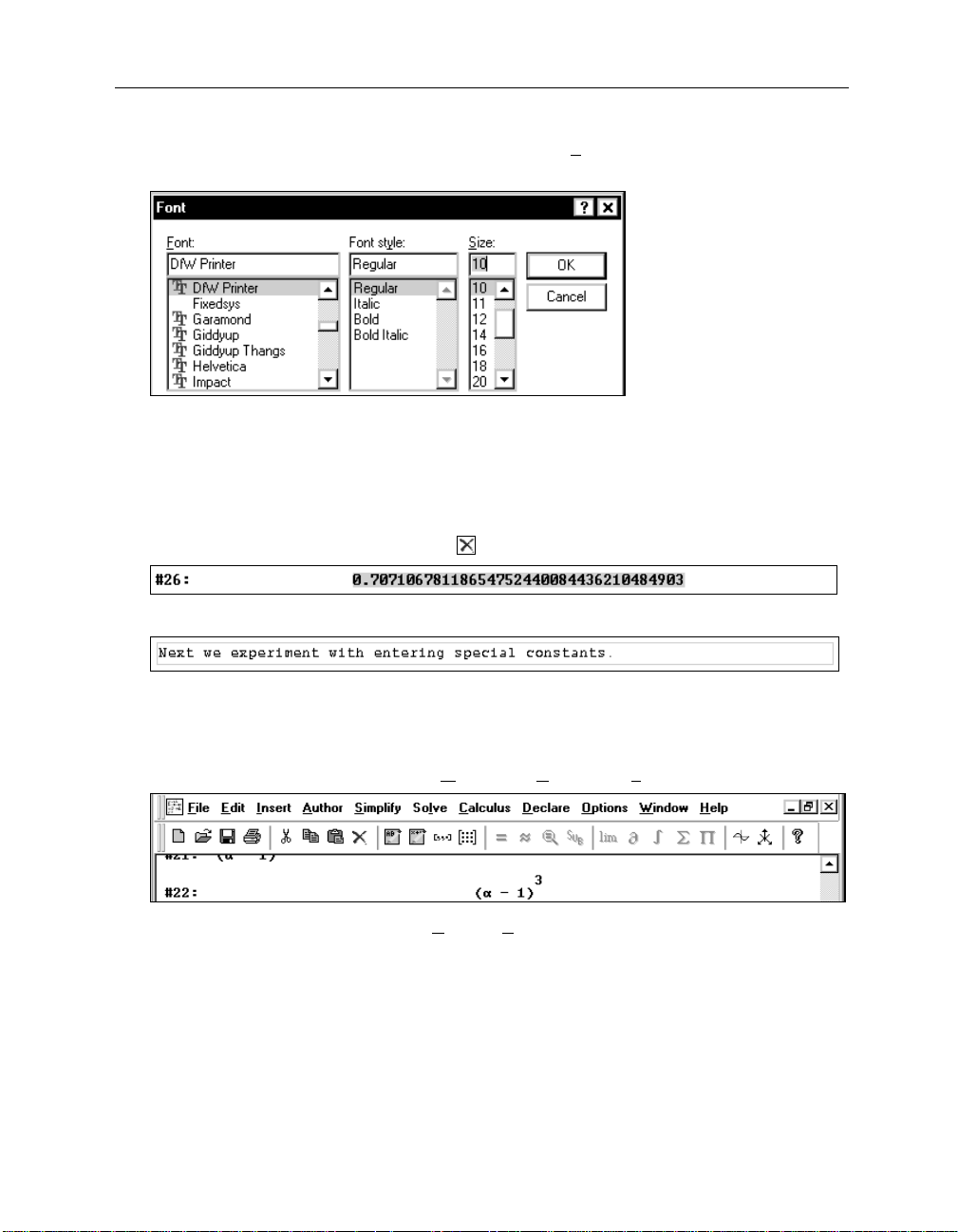
Change the font size to 10 points by scrolling within the
Size
selection menu appropriately,
then selecting the number 10, or by overwriting 12 with 10 via the keyboard.
Close the dialog with
(_OK_)
.
When continuing to write into the text object you started (you may need to click into the text
object to put it into text editing mode), it still is in 12 point size, because the setting you just
changed effects
Delete the text object for a retry with the new default text font size. Select it by clicking into
it then using
Enter a new text object with the following contents:
new
text objects only.
(Esc)
. Delete with
(Del)
or
.
The text has font size 10 points now. You will not need the Formatting Toolbar any more in this
session, so switch it off to provide more space for other purposes. Switching a toolbar off
requires the same procedure as switching it on.
Turn the Formatting Toolbar off using
Window>View Toolbars>Formatting Toolbar
.
Experiment with the commands from the
changing the “look” of a D
ERIVE
worksheet.
Options>Display
submenu to become familiar with
Kutzler & Kokol-Voljc: Introduction to D
519
ERIVE
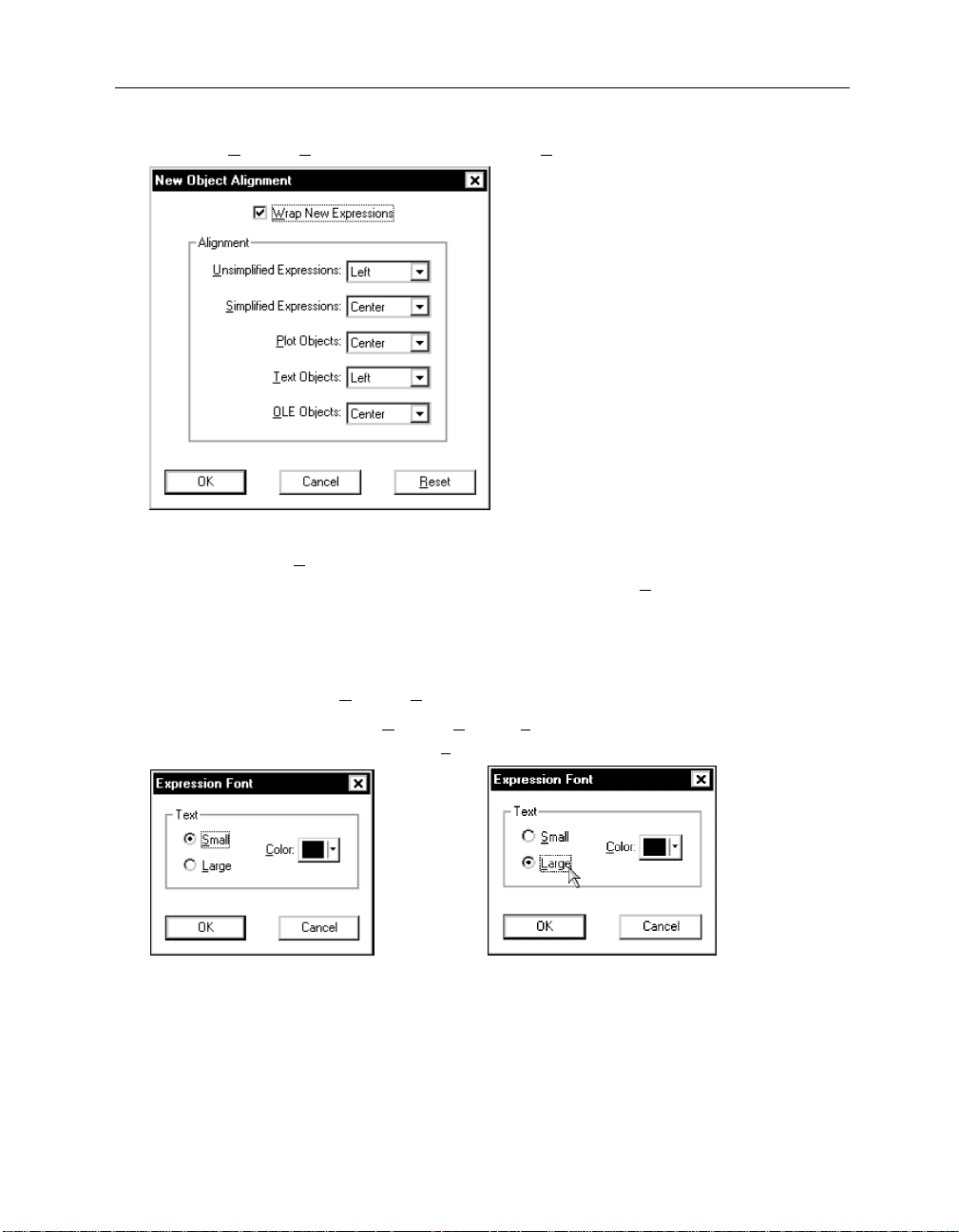
Select the
Options>Display
menu’s first choice (i.e.
Alignment of New Objects
.)
This invokes a dialog box that allows you to control the alignment of all the objects that can be
ERIVE
in a D
worksheet.
obtained by adding an operator to an expression without simplifying.
Unsimplified Expressions
are expressions entered by you or expressions
Simplified Expressions
expressions obtained from simplifying or approximating an expression. It is helpful to display
user input left justified and the answers centered, as it is done by the default setting.
To keep the settings as they are, exit the dialog with
Try the next command in the
Try the menu’s second choice,
change the text size by clicking on the
Options>Display
Options>Display>Font of All Expressions
Large
(_Cancel_)
submenu.
radio button.
or the
(Esc)
key.
(left picture), then
are
20 Chapter 1: First Steps
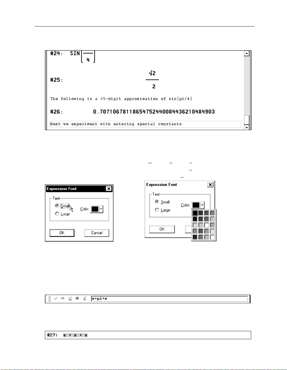
Carry out the change by leaving the dialog box with
(_OK_)
.
This font is useful for demonstration purposes, especially when using an overhead projector with
a display palette. For personal work the small font may be preferable. Therefore, switch back to
it and try a different color instead.
To undo the change of expression size, select
again, then change the text size back to small by clicking on the
picture.) Prepare for changing the font color by opening the
Options>Display>Font of All Expressions
Small
radio button (left
Color
selection menu.
Select a color of your choice by clicking on it, then close the dialog with
(_OK_)
.
Earlier you entered π via the Greek or Math Symbol Toolbar. There are several methods for
entering special constants such as π, the base of the natural logarithm e, or the imaginary unit i.
To enter a sum of three π‘s, first move the focus into the entry line using
π
from one of the two symbol toolbars, the second one by typing pi, and the third one as
(Ctrl)+(P)
. (The pluses in between are all entered via the keyboard.)
(F2)
. Enter the first
These are the three methods of entering the number π. While some look different in the entry
line, they all look and mean the same once they are entered:
Conclude the input of the sum of three π‘s with
(¢)
.

Kutzler & Kokol-Voljc: Introduction to D
521
ERIVE
There are also three methods for entering the base of the natural logarithm e. Use all three of
them to enter a sum of three e’s, then add the ordinary letter e to see the difference between a
variable with this name and the famous constant. There is also another method of simplifying an
expression.
Enter the first e from the Math Symbol Toolbar using
the third one as
(Ctrl)+(E)
. Then type:
+e=
(Note the use of the postfix equals operator.)
, the second one by typing #e, and
End the input of the sum of three e’s and the variable e with
(¢)
.
The postfix equals operator causes an automatic simplification and the generation of an equation
whose left hand side is the unsimplified expression and whose right hand side is the simplified
expression. This method displays both the unsimplified and simplified expression on the same
line, saving lines on the screen.
Similarly there are three methods for entering the imaginary unit. You can obtain I from the
Math Symbol Toolbar, type #i, or enter it via the key combination
(Ctrl)+(I)
.
Conclude this chapter as follows.
Enter the text “
ERIVE
Exit D
. The
ERIVE
Exit D
To exit without saving the worksheet, select
This is the end of the first chapter.
Exit
command can be found in the
using the
File>Exit
command.
(_N
File
o_)
”
menu.
.

22 Chapter 1: First Steps
Summary
Algebra Window
(Del)
or
or
or
or
or
File>Exit
Simplify>Expand
Options>Display
Window>View Toolbars>Formatting Toolbar
(½), (¼)
(Esc)
click left mouse button into row occupied by the expression ......................... highlight expression
click left mouse button into text object .................................................. edit contents of text object
click onto text object frame or left or right of it, or press
............................................................................................. delete highlighted expression
Insert>Text Object
Author>Expression
implify>Basic
S
implify>Approximate
S
.................................................................................................................................. exit D
................................................................................. expand highlighted expression
............................................................................................... change display settings
........................................................................ move highlighting one expression up, down
............................................................................................................................. cancel command
.....................................................................highlight text object (without text editing)
(F5)
or
......................................................................... simplify highlighted expression
............................. insert text object after the highlighted object
(F2)
or
............................. enter expression, move focus into entry line
................................................... approximate highlighted expression
.................................... toggle the formatting toolbar
(Esc)
from within text editing ...............
ERIVE
Expression Entry Toolbar
(¢)
or
................................................................................................................ enter simplified expression
...................................................................................... enter expression and simplified expression
(Esc)
(ÿ)
or
or
or
, etc................................................................................................................................... Greek letters
or
=
(postfix equals operator) ................................................................................ enforce simplification
...................................................................................................................... enter expression
............................................................................................ move focus into the algebra window
...................................................................................................... highlight contents of entry field
(Ctrl)+(P)
(Ctrl)+(E)
(Ctrl)+(I)
(Ctrl)+(Q)
or pi ...........................................................................................................................
or #e .............................................................................. base of natural logarithm
or #i ................................................................................................. imaginary unit
sqrt
or
..................................................................................... square root symbol
π
e
i

Chapter 2: Documenting Polynomial Zero Finding
The emphasis in this chapter is on creating a simple mathematical document about the finding of
the zeros of a polynomial. At the same time you will learn the corresponding basic techniques of
ERIVE
using D
Start D
.
ERIVE
.
Your first session with D
information about the status of D
performed with the
this file. The
default settings or start D
changes from the first chapter. This book is written so that each chapter starts with a factory
default D
Start with a factory default D
Start the new document with an appropriate headline.
Insert a text object containing the text “
You will look for the zeros of the polynomial
Derive Startup
ERIVE
. We recommend that you do the same.
ERIVE
left a trace in the form of an initialization file. This file stores
ERIVE
before you last shut it down. For example, the change
Options>Display>Font of New Text Objects
dialog gives you the choice to either start D
ERIVE
with the settings from the initialization file, i.e. with some of the
ERIVE
by exiting the dialog with
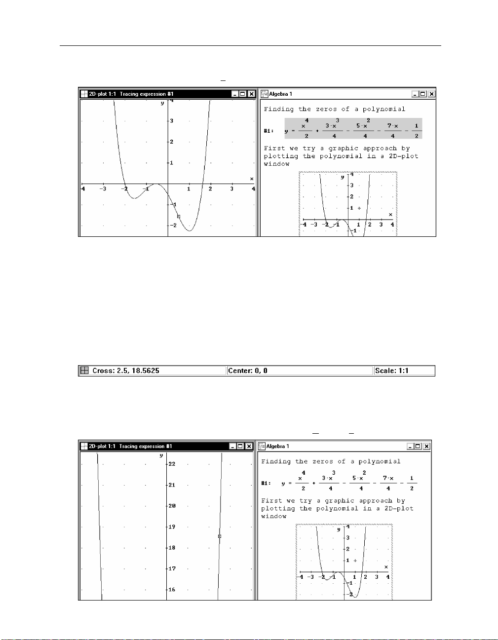
Finding the zeros of a polynomial
432
xxxx
=+ − −−
()ypx
y
,
24 442
=
command is among the data in
ERIVE
with the factory
(_Y
es_)
.
.”
3571
.

24 Chapter 2: Documenting Polynomial Zero Finding
Enter the above polynomial by preparing for expression input with
, then typing:
y=x^4/2+3x^3/4-5x^2-7x/4-1/2
(Intentionally leave out the /4 in the middle term.)
From here on, the key
(¢)
or the button
(_OK_)
will be displayed only in ambiguous situations.
It will not be used any more for simple inputs such as the above. It is important for some of the
features you are going to study and use in this chapter that you work with the above polynomial.
Therefore, make sure it was entered properly.
As you know, it was not! The /4 in the middle term is missing. This is easily repaired by applying
Edit>Derive Object
the
Edit the highlighted expression by selecting the
command to the highlighted expression.
Edit>Derive Object
command.
This brings a copy of the expression into the entry line with the cursor positioned at its left end,
so the system is ready for editing.
Insert /4 after
(¢)
The
key performed a
5x^2
, then end the input with
replacement
of the old expression with the new one. There is no need
to delete the old expression when using the
(¢)
.
Edit>Derive Object
command.
Consider looking at a house from several different positions. From each position you will see
details that you can’t see from other positions. Based on this idea, mathematicians use a variety
of different representations for mathematical objects. The fourth degree polynomial that you
entered is displayed as an
algebraic
representation. Next you will produce a
graphical
representation, because this representation is particularly useful for obtaining information about
1
the zeros. In other words, you will plot
its graph.
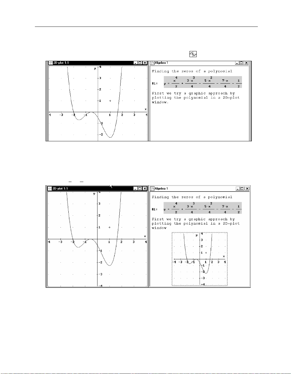
Since the major goal in this session is to properly document the mathematical work, . . .
. . . insert the text
“First we try a graphic approach by plotting the polynomial in a 2D-plot
window.”
1
“Plot” is a technical term. As such, it includes different aspects of drawing and graphical
representation. It does not stand for mathematical accuracy, and in this book it will be used with three
different meanings: for the activity of producing a graphical representation, for a graphical
representation as an object, and for the corresponding D
ERIVE
command.

Kutzler & Kokol-Voljc: Introduction to D
525
ERIVE
Prepare for plotting a 2D graph: Open a 2D-plot window by clicking on the
button
or selecting the
ERIVE
D
created a plot window, so that you now have two windows to work with: an algebra
window and a 2D-plot window. Use the usual W
Window>New 2D plot Window
INDOWS
techniques to flip between windows or
command.
change their sizes and positions.
Put the two windows side by side using the
Window>Tile Vertically
command.
2D-plot Window
Each window is labeled with the window type in its upper left corner (
2D-plot
and
Algebra
). The
active window’s Title Bar is dark; the inactive window’s Title Bar is dimmed. Since the plot
window is active, the Menu Bar, the Command Toolbar, and the Status Bar are all different from

26 Chapter 2: Documenting Polynomial Zero Finding
that of the algebra window. In particular, the Status Bar displays the following graphics
information:
Cross
•
•
•
•
gives the coordinates of a movable cross,
Center
gives the coordinates of the picture center,
Scale
gives the scale factors of both axes,
The crossed square icon preceding the word
Cross
indicates Cartesian coordinates.
Draw the graph using the
Oops—the
Plot Expression
The reason is that the
Plot Expression
Plot Expression
button .
button is dimmed inaccessible.
button (as well as its equivalent, the
Insert>Plot
command) plots the point set given by the algebra window’s highlighted expression, but
currently the second text object is highlighted and a text object can’t be plotted.
Highlight the polynomial by clicking on it (this makes the algebra window the active
window), then make the 2D-plot window active again by clicking its Title Bar.
There are several techniques to make a different window active:
•
From the algebra window use the Command Toolbar’s
the 2D-plot window use the Command Toolbar’s
•
Click on the window you want to make active. This method, however, must be used with
2D-plot window
Algebra window
button and from
button .
care: Clicking on an algebra window with the left mouse button is likely to alter the
highlighting, clicking on a 2D-plot window with the left mouse button is likely to move the
graphics cross, this might have unexpected effects. Therefore, it is better to click with the
right mouse button to change windows, or to click, with any mouse button, into the window’s
Title Bar.
•
From the algebra window use the
window use the
•
From the algebra window use the
(Alt)+(W)
the
Window>x Algebra
(x)
and
keys as abbreviations of the above.
Window>y 2D-plot
command and from the graphics
command. (The numbers x and y may vary.)
(Alt)+(W)
and
(y)
keys and from the graphics window use
Kutzler & Kokol-Voljc: Introduction to D
527
ERIVE
Now the
Plot Expression
button is available, and you are ready to plot the polynomial.
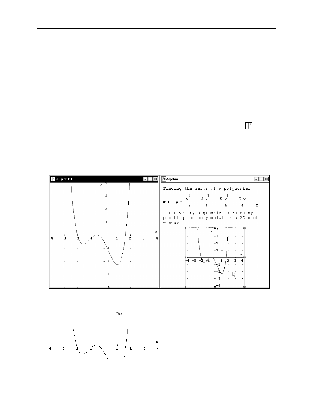
Draw the polynomial’s graph using the
Plot Expression
button .
Now we have both an algebraic and a graphical representation of the polynomial available.
However, the graphical representation is
outside
the algebra window’s worksheet in its own
independent plot window.
Copy the current plot window into the algebra window’s worksheet by using the 2D-plot
window’s
File>Embed
command.
This “freezes” the current status of the plot window into the worksheet. The plot window is
interactive; the embedded plot image is not. The embedded plot image can be brought back into
an interactive plot window at any time with a double mouse click.
The graphical representation is useful for exploring the polynomial’s zeros. However, from the
current picture it is not clear whether the polynomial has two, three, or four distinct zeros. An
answer can be found by inspecting the graph with the moveable graphics cross. Its coordinates
are displayed in the status line, which now shows the cross at the initial position (1,1):
28 Chapter 2: Documenting Polynomial Zero Finding
The color of the cross can be changed using the
Options>Display>Cross
command.
When the plot window is active, the cross can be repositioned by either moving the mouse
pointer and clicking the left mouse button or by using the arrow keys
Move the mouse pointer to (1,-1), or near it, then click with the left mouse button to move
(Æ), (æ), (½)
, and
(¼)
the cross to this position (left picture). Use the arrow keys to move the cross to (0.5,0.5). Try
(Ctrl)+(Æ), (Ctrl)+(æ), (Ctrl)+(½)
(Ctrl)+(¼)
, and
to move the cross in bigger
steps.
(Home)
The
key moves the cross to the plot window center.
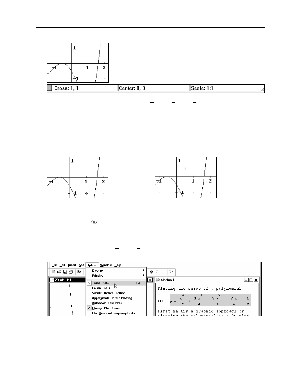
The trace mode is very useful for inspecting curves. This mode can be switched on and off with
Trace Plots
the
(F3)
. As is customary in W
button , the
Options>Trace Plots
INDOWS
programs, a button with the same effect as a command is
command, or the corresponding hot key
displayed in the respective menu left of the command, while the hot key is displayed right of the
command. Check this out for the
Open the
Options
menu.
Options>Trace Plots
command:
.
Kutzler & Kokol-Voljc: Introduction to D
529
ERIVE
Turn trace mode on by selecting the
Trace Plots
command.
When trace mode is switched on, the cross changes its shape into a square and jumps vertically
to the curve, with its horizontal coordinate unchanged. The expression number of the traced
curve is displayed in the plot window’s Title Bar (here:
mode is switched on, the square can be moved only along the curve. This can be done using
and
(æ)
, or using
(Ctrl)+(Æ)
(Ctrl)+(æ)
and
Tracing Expression #1
). When trace
(Æ)
for “big steps.” It can also be done by moving
the mouse pointer and clicking with the left mouse button to the new position. If there are
several graphs displayed, use
Become familiar with moving the square. Use the arrow keys and the mouse to move the
(½)
and
(¼)
to select another graph.
square. Finally, click the left mouse button at the point (2.5,0).
What happened to the square? It disappeared. Looking at the status line indicates the reason. The
square’s vertical coordinate is 18.5625, so it is far from the current plot area. You can ask D
ERIVE
to move the plot area where the cross or square is.
Move the plot area where the cross is by flipping the switch
Options>Follow Cross
.
30 Chapter 2: Documenting Polynomial Zero Finding
The plot window “follows” the square. This means that the plot ranges for the horizontal and the
vertical axes are changed automatically to ensure that the cross is visible. Since this mode can
destroy a chosen plot range, follow mode should be used carefully and is therefore switched off
by default.
Turn follow mode off by selecting
Options>Follow Cross
again.
There are several ways to restore a previous range:
•
While follow mode is on, you can click the left mouse button at a horizontal position where
the corresponding vertical curve coordinate is within the original plot range. This requires
some knowledge and reasoning about the curve.
•
Independent of the follow mode status you may use the
•
Select the
Set>Plot Range
Set>Plot Region
or the
Center on origin
command, use the
button .
(_Reset_)
button,
then leave the dialog.
•
If available, double click on an embedded version of the original graph. This last option is
particularly convenient.
Restore the original graph by double clicking on the embedded graph.
Trace mode was lost because the embedded graph was produced before trace mode was turned
on. Switch trace mode on again to start looking for the polynomial’s zeros.
Switch trace mode on with
, then move the square to the rightmost zero, as near as you
can get to the horizontal axis.
ERIVE
D
displays the square coordinates as
different.) Using the left arrow key
Cross: 1.62, 0.01688368
(æ)
once moves the square to
. (Your numbers might be
Cross: 1.6, -0.1512
. You have
Kutzler & Kokol-Voljc: Introduction to D
531
ERIVE
not found a position at which the y-coordinate is zero, but you can say that the polynomial zero
must be between 1.6 and 1.62, probably being closer to 1.62. An obvious approach for getting
closer is magnification.
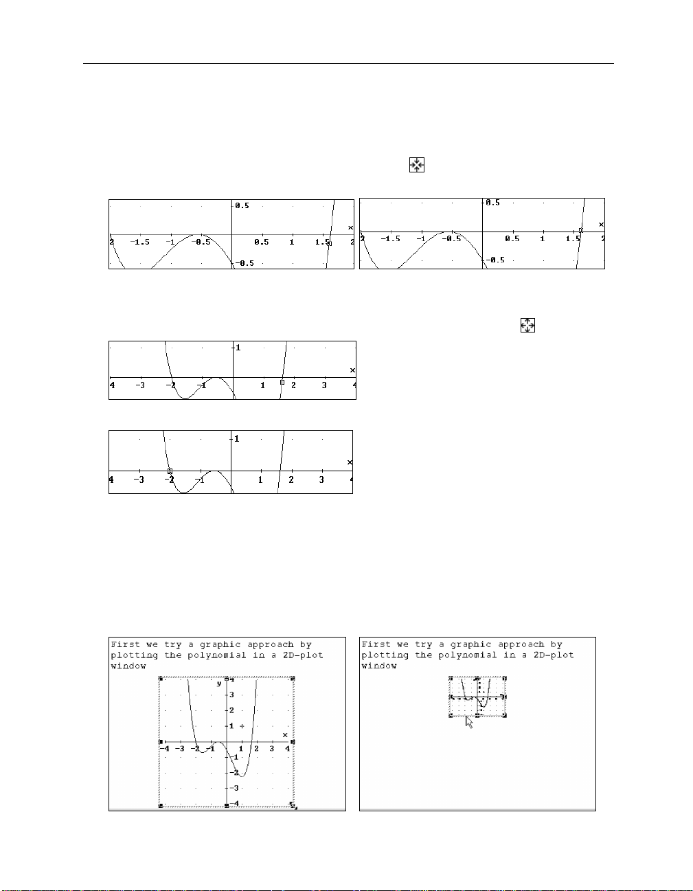
Zoom in using the Command Toolbar’s
Zoom in
button (left picture), then move the
square closer to the rightmost zero.
Now you get
Cross: 1.62, 0.01688368
Cross: 1.61, -0.06817304
and
(or whatever numbers you
obtain) hence the polynomial zero is between 1.61 and 1.62.
Restore the original scale factors by zooming out with the
Find an approximation for the leftmost zero by moving the square to it.
Zoom out
button .
The leftmost zero seems to be at exactly x=-2.
Document what you found so far by inserting appropriate text objects.
Switch to the algebra window. Resize the embedded plot: Select the image by clicking on it.
The image is surrounded by 8 black squares, which can be used to resize it. Move the mouse
pointer to the lower right corner until a double-headed arrow appears. Press and hold the
left mouse button. With the left mouse button held down, drag the pointer towards the
image center. When a suitable size is reached, release the mouse button.
32 Chapter 2: Documenting Polynomial Zero Finding
When you don’t like the change of the aspect ratio such is in the above pictures, you can easily
restore it. You will learn how to do this in Chapter 4.
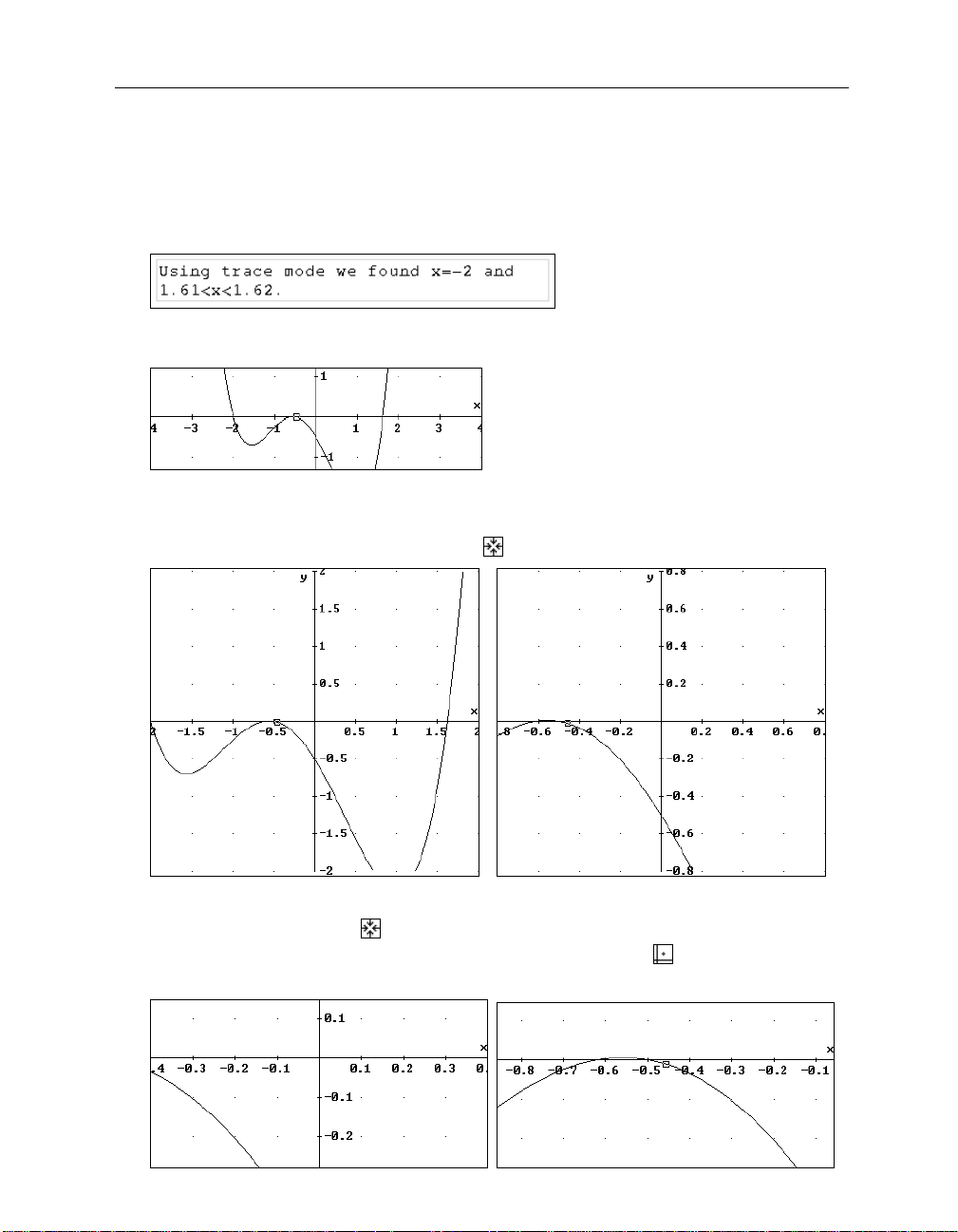
Insert a text object documenting the method and result of your findings.
Insert a new text object and enter the following text (use the numbers you found):
Search for more zeros: Make the plot window active, then move the square to the uncertain
middle section.
You will find that there is one zero between -0.62 and -0.6. Another zero seems to be at exactly
x=-0.5. To obtain a picture with intersections of the graph, magnify again.
Zoom in, this time using the
Zoom in
button twice.
It becomes obvious that there are two zeros. Continue to magnify the graph.
Zooming in once more with
switched off (left picture). The very useful
lets the square leave the plot window because follow mode is
Center on cross
button shifts the plot range
so that the square/cross is in the center of the new plot image.
Kutzler & Kokol-Voljc: Introduction to D
533
ERIVE
Move the square to get a better approximation of the left zero.
Move the square near the left zero and note the cross coordinates in the Status Bar.
Now the change of sign happens between x=-0.62 and x=-0.618. Produce a graph with steeper
intersections to get a more accurate answer.
Zoom in vertically only, using the
Zoom vertical in
button .
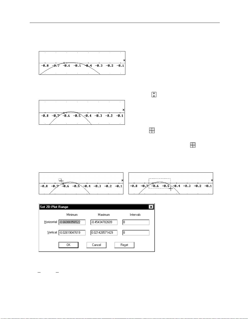
A highly recommended tool is the
Set range with box
button , which allows to choose a crop
rectangle graphically.
Prepare for choosing a crop rectangle by using the
Set range with box
button .
The mouse cursor turns into a crosshair.
Choose a crop rectangle: Click and hold the left mouse button at the top left corner of the
desired area. Drag the mouse down and to the right until the box encloses the desired area.
Release the mouse button.
Set 2D-Plot Range
The
dialog box is displayed, reflecting the numerical equivalents of the
choices you just made with the mouse. This dialog box could be obtained in the first place using
Set>Plot Range
the
command. But a graphical choice of the plot range is often more convenient.
34 Chapter 2: Documenting Polynomial Zero Finding
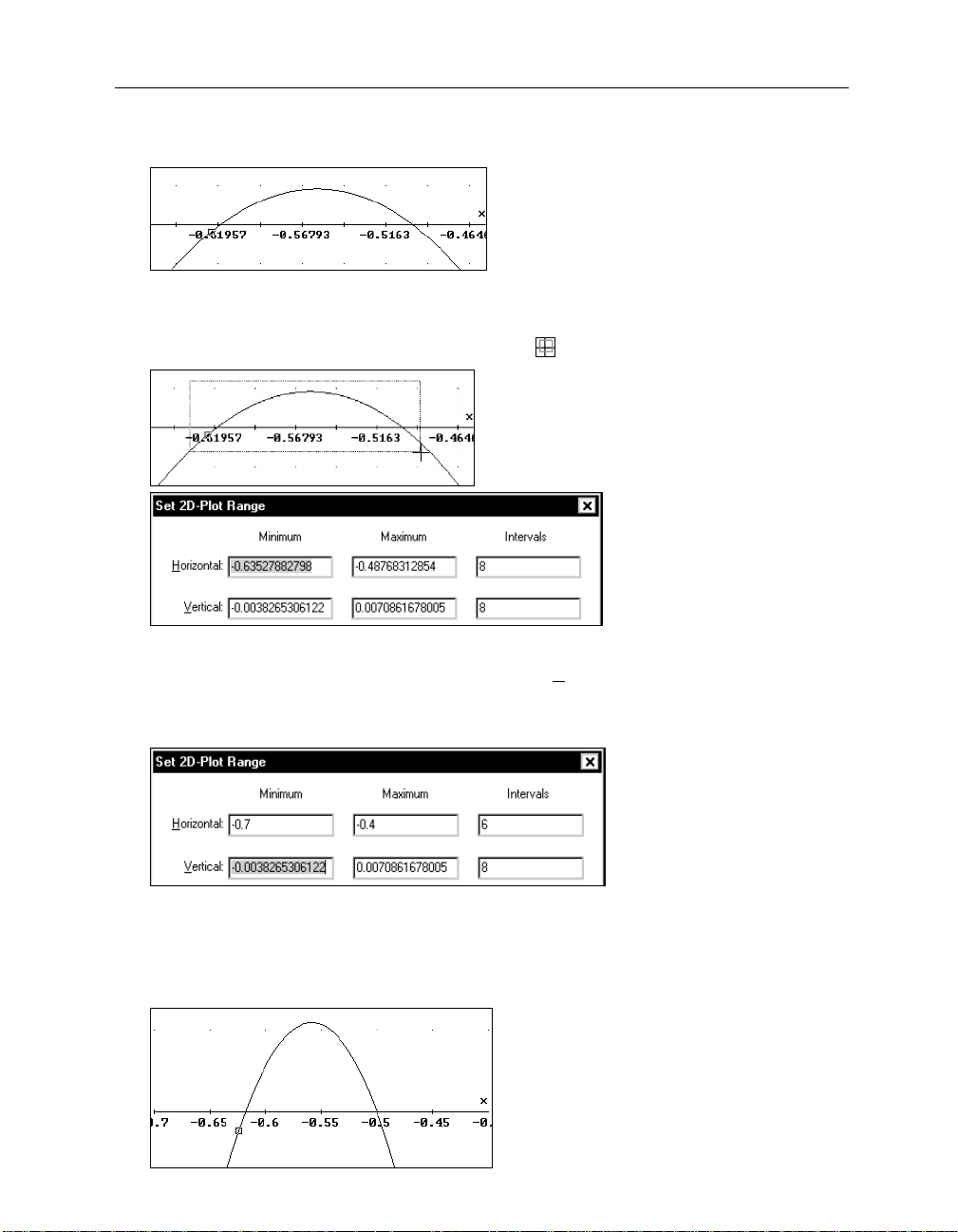
See what happens if you confirm with
(_OK_)
.
Notice the complicated numbers below the tick marks (your numbers are likely to be different)
and in the Status Bar scale factors. This is caused by the graphical box selection.
Zoom in again using the
Set range with box
button .
It is helpful to edit the suggested numerical values to the nearest simple values. Start by
overwriting the highlighted value of the input field for the
(ÿ)
key
-0.7
to make the next input field active. Enter the following values.
(ÿ)
-0.4
(ÿ)
6
(ÿ)
Horizontal Minimum
. Then use the tab
Make the values for the
Maximum
the
fields. For example, 6 intervals for a horizontal range of length 0.3 (= difference of
Intervals
fields fit to the difference of the values for the
-0.7 and -0.4) ensures nice numbers below the tick marks.
-0.01
(ÿ)
0.01
(ÿ)
4
(_OK_)
Minimum
and
Kutzler & Kokol-Voljc: Introduction to D
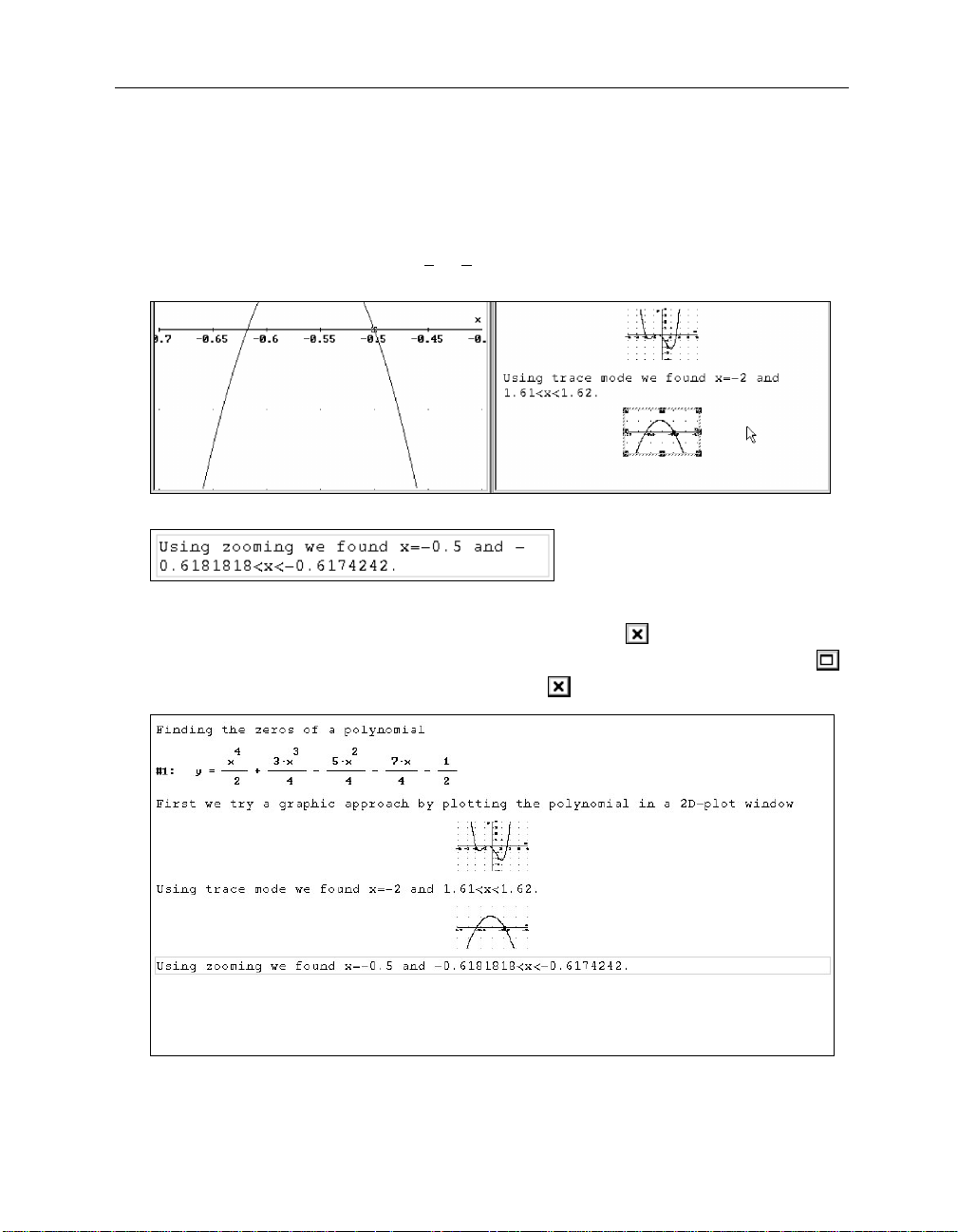
Use the trace mode square to find approximations of the two zeros.
535
ERIVE
The left zero lies between -0.6181818 and -0.6174242; and the other zero probably is at -0.5. All
the above work now should be documented in the algebra window’s worksheet by embedding
the graph and adding an appropriate text object.
From the 2D-plot window select the
File>Embed
command, then switch to the algebra
window and resize the embedded plot appropriately.
Insert a new text object documenting the method and result of your findings:
Close the plot window, then open the algebra window to full size.
Close the plot window by clicking the left mouse button on the
button that is located in
the window’s upper right corner. Open the algebra window to full size by clicking on the
button, which is located left of the algebra window’s button.
Next compute the zeros by solving the corresponding polynomial equation. Before doing so,
enter an appropriate textual description of your approach.
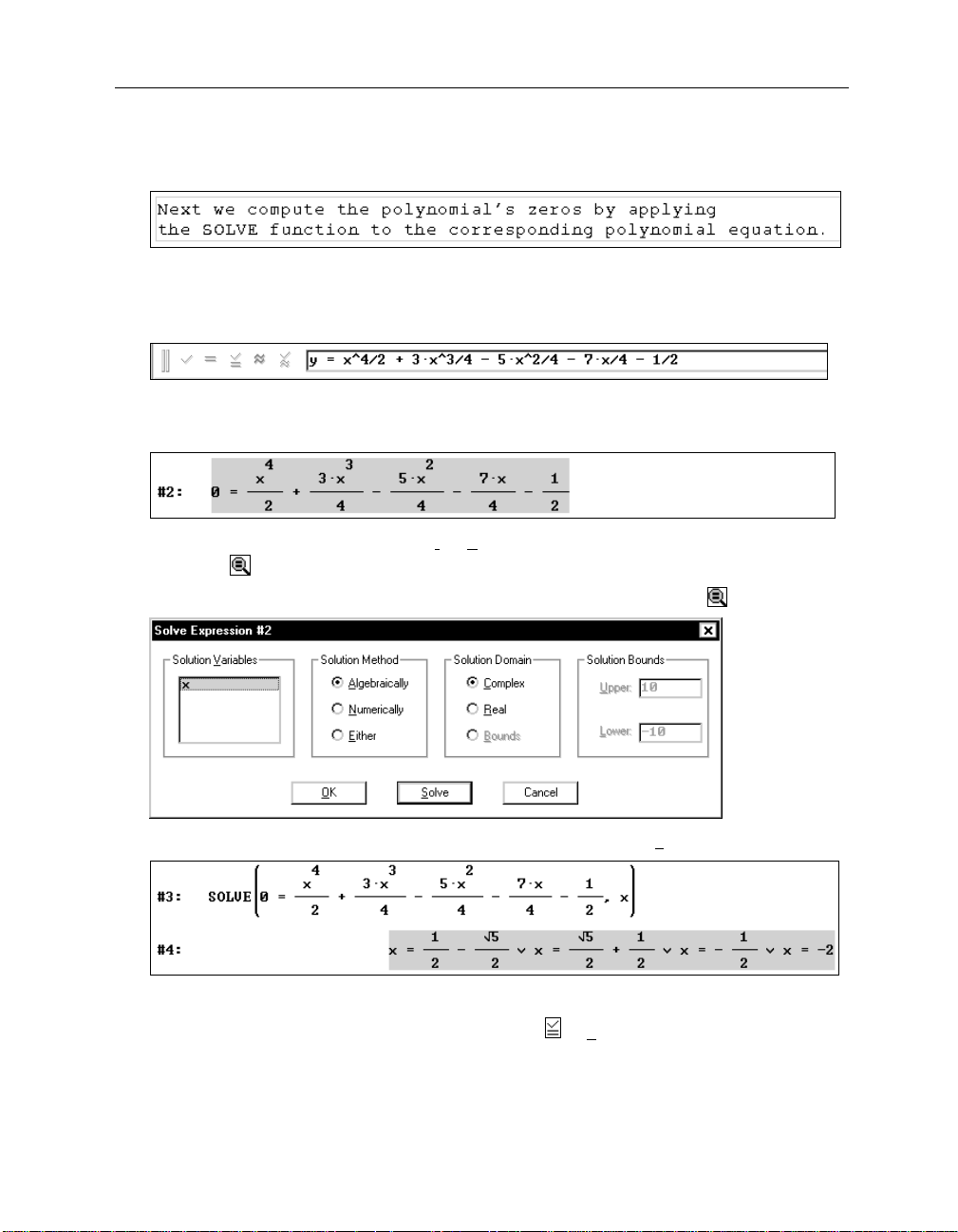
36 Chapter 2: Documenting Polynomial Zero Finding
Enter the text: “
to the corresponding polynomial equation.
Next we compute the polynomial’s zeros by applying the SOLVE function
”
Generate the corresponding polynomial equation.
Highlight the polynomial #1, move focus into the entry line with
(F2)
(which is the hot key
for authoring expressions), then auto-paste a copy of the polynomial using the hot key
(F2)
may become your most frequently used hot key.
Replace y with 0 then conclude the input with
For solving this equation either use the
Solve>Expression
(¢)
.
command or the corresponding
toolbar button .
Prepare for solving the equation by applying the
Solve Expression
button .
(F3)
.
(_S
Solve the equation. Accept all suggested parameters by selecting
olve_)
Here ∨ is the mathematical symbol for the logical operator OR.
(_S
Similar to the Entry Toolbar’s
Enter and Simplify
button ,
unsimplified expression (which is the formal application of the
olve_)
generated both an
SOLVE
function to the equation)
and a simplified expression (which is the solution of the equation.) The exit
generated the unsimplified expression only.
.
(_OK_)
would have

Kutzler & Kokol-Voljc: Introduction to D
537
ERIVE
Enter the text “
Expression #4 gives the four exact zeros of the polynomial.
”
In order to compare these results with what you found graphically, approximate expression #4.
Before doing so, again add a textual description of your approach.
Enter the text “
graphically.
Approximate expression #4 by first highlighting it, and then applying the
We approximate #4 so that we can compare it with what we found
”
Approximate
button .
To turn this worksheet into a good piece of mathematical documentation, do some more editing,
then print and save it. First, add a signature documenting author(s) and date.
Switch the Formatting Toolbar on using
Window>View Toolbars>Formatting Toolbar
.
All fields and buttons are dimmed as long as there is no text object in editing mode.
Add a text object at the end of the worksheet using
. Choose a special format for the
signature: In the Formatting Toolbar change the font size to 8 points and click on the
Right Justify
button .
This document was created by . . . on . . ..”
Enter “
Next change the topmost text object into an attention-catching title line.
Highlight the first text object’s contents using the usual text processing techniques.
Choose a format that is suitable for a title line, for example . . .
. . . change to 14 point font size, bold (
Switch the Formatting Toolbar off using
), centered ( ), then add a blank line.
Window>View Toolbars>Formatting Toolbar
.

38 Chapter 2: Documenting Polynomial Zero Finding
Before sending a document to the printer, it is a good idea to do a print preview.
Look at the print preview using the
File>Print Preview
command.
Print preview offers various options including a button for zooming in.
Zoom in with
(_Zoom_I
n_)
.
The magnifying glass shaped cursor in the upper right quarter of the page indicates that an
alternative to using the
(_Zoom_In_)
button is to click with the left mouse button.

Kutzler & Kokol-Voljc: Introduction to D
539
ERIVE
Make the expressions slightly larger. Change the expression font size via the
Options>Printing
submenu.
Prepare for changing the expression font size: Close the print preview window with
(_C
lose_)
, then select the command
Here you can select the expression font size, choose between
the printing of
Change the font size to 11 points, then close the dialog with
Apply again the
Annotation
File>Print Preview
Computation Time
s and
Options>Printing>Expression Layout
Regular
and
Bold
s. (By default neither is printed).
(_OK_)
.
command, this time zooming in twice.
.
font, and control
The worksheet is now ready to be printed.

40 Chapter 2: Documenting Polynomial Zero Finding
(_P
Prepare for printing the document using print preview’s
rint_)
button.
Make sure that the printer is properly connected, switched on, and set. In the
you can change the printer or the printing properties, change the print range from
Printing
All
dialog box
to either a
range of pages or the highlighted expressions, or change the number of copies from the default 1
to the number you want.
Send the document to the printer with
(_OK_)
.

Kutzler & Kokol-Voljc: Introduction to D
541
ERIVE
Saving the worksheet preserves your work for later use or modification.
Save the worksheet by selecting the
File>Save As
command.
ERIVE
D
suggests storing the file in the subdirectory
Math
. You may choose a different directory
by selecting one from the selection menu that is offered for the
Accept the suggestion and enter the file name
(_S
Close the dialog with
ave_)
.
Notice the Title Bar. Previously there was
Algebra 1 chapter02.dfw
worksheet. Now there is
chapter02.dfw
. The suffix
[
.dfw
is the default that is chosen when you do not specify a suffix as
[
chapter02
Algebra 1
]
as the indication of an unnamed algebra
]
, indicating an algebra worksheet with name
part of the filename.
Exit from D
ERIVE
.
Save in
in the
field.
File name
input field.

42 Chapter 2: Documenting Polynomial Zero Finding
Summary
Algebra Window
Solve>Expression
or
............................................................................................ open 2D-plot window or switch to one
........................................................................................................... right justify highlighted object
.................................................................................................................... center highlighted object
File>Save As
File>Print Preview
Edit>Derive Object
Options>Display>Cross
Options>Printing>Expression Layout
Window>New 2D plot Window
double-click left mouse button on embedded plot ................. open embedded plot in plot window
.......................................................................................... save worksheet using a name
............................................................................................................ print preview
or
(Ctrl)+(ª)+(E)
or
double-click left or right of expr. ...................... edit highlighted expression
.......................................................... change appearance of graphics cross
................................................................. open new 2D-plot window
............................................................. solve equation
...................................................... format expression layout
2D-plot Window
Insert>Plot
or
Options>Trace Plots
or
................................................................................................................. center plot region on cross
................................................................................................................ center plot region on origin
(F9)
or
(F10)
or
(F7)
or
.................................................................................................. graphically choose a crop rectangle
File>Embed
Set>Plot Range
Options>Follow Cross
(Æ), (¼),(æ), (½)
(Ctrl)+(Æ), (Ctrl)+(¼), (Ctrl)+(æ), (Ctrl)+(½)
(Home)
............................................................................................. move cross to plot window center
...................................................................................... plot highlighted expression
(F3)
or
......................................................................................................................................zoom in
................................................................................................................................. zoom out
.................................................................................................................... zoom in vertically
....................................................................... copy plot window into algebra worksheet
................................................................................................... set plot range borders
........................................................................................... toggle follow mode
................................................. move cross one pixel (one dot) on the screen
......................................................................... toggle trace mode
......................... move cross several pixels
All Windows
Window>Tile Vertically
................. arrange windows as right-left split (active window on the left)

Index
22
............................................................. 124
.............................................................. 35
.............................................................. 35
5x – 6 = 2x + 15 ......................................... 63
=−
zx y
cos( )zxy
=⋅
∨
........................................................... 67, 75
∧
................................................................. 75
° ................................................................ 147
:∈ ...................................................... 137, 138
:= .......................................... 66, 96, 138, 167
∞
............................................................... 138
↓
............................................................... 161
(¢)
(¼)
(½)
(ª)+(¼)
(ª)+(½)
(ª)+(Æ)
(ª)+(æ)
(Æ)
(æ)
(Alt)+(PrtSc)
(Ctrl)+(¢)
(Ctrl)+(¼)
(Ctrl)+(½)
(Ctrl)+(ª)+(¼)
(Ctrl)+(ª)+(½)
(Ctrl)+(ª)+(M)
(Ctrl)+(Æ)
(Ctrl)+(æ)
(Ctrl)+(C)
(Ctrl)+(E)
(Ctrl)+(P)
(Ctrl)+(Q)
(Ctrl)+(V)
(Ctrl)+(X)
(Del)
............................................. 117
................................. 125, 132
..................................................... 4, 106
.................................. 6, 28, 29, 118, 209
.................................. 6, 28, 29, 118, 209
.......................................... 45, 121
.......................................... 46, 121
.......................................... 46, 121
.......................................... 46, 121
......................................... 5, 28, 29, 118
......................................... 5, 28, 29, 118
...................................... 201
.............................. 11, 64, 106
............................................ 28
............................................ 28
................................... 53
................................... 53
................................... 201
...................................... 28, 29
...................................... 28, 29
...................................... 54, 201
.............................................. 20
.............................................. 20
.............................................. 11
.............................................. 54
...................................... 54, 201
........................................................... 5
(Esc)
........................................ 5, 13, 16, 243
(F2)
.................................................... 11, 126
(F3)
........................................ 28, 36, 49, 122
(F4)
...................................................... 49, 64
(F9)
.......................................................... 128
(Home)
........................................................ 28
(PgDn)
...................................................... 119
(PgUp)
...................................................... 119
(PrtSc)
(ÿ)
(Insert expression)
.dfw
2:1
2D-plot Window
3D-plot window
.................................................... 201
...................................................... 11, 34
............................. 49, 64
............................................................. 41
............................................................... 56
button ..................... 25
button ..................... 117
A
abort computation .................................... 90
absolute value function .... 74, 139, 154, 198
accuracy ..................................................... 86
activate window ........................................ 26
aggressive simplification ....................... 151
algebra window ..................................... 3, 25
Algebra Window
algebraic equation .................................. 232
algebraic representation .......................... 24
Algebraically
algebra-state variable ................... 66, 68, 84
algorithmic limitations ............................. 87
aliasing ..................................................... 133
Alpha .......................................................... 12
alternative to
analytic geometry ................................... 185
AND
.............................................................. 75
ANGLE
........................................................ 155
angle between two vectors .................... 154
Angular unit
annotation ................................................ 105
button .................... 26
radio button ....................... 91
Edit>Derive Object
............................................ 148
........... 78
270 Index
annotation of expression .......................... 6
annotation’s position ............................. 106
apostrophe ................................................ 51
Apply parameters to rest of plot list
... 175
applying differentiation ......................... 207
Approximate
button ............................ 6
approximate computations ................... 230
approximate mode ................................... 83
approximate step by step ........................ 88
approximation tools ................................. 83
arbitrary number of digits ....................... 83
area .......................................................... 212
aspect ratio ....................................... 31, 115
assignment expression ...................... 66, 96
assignment operator .............................. 138
Asterisk
................................................... 247
audit trail ................................................... 66
Author and Simplify
Author Expression
Author Expression
Author Matrix
Author Vector
Author>Expression
Author>Matrix
Author>Vector
Auto Plot Color
button ................. 8
button .................. 4
button .................. 8
button ....................... 162
button ...................... 153
................................. 13
........................................ 162
........................................ 153
scheme ........................ 125
automatic color cycling mode .............. 156
automatic renumbering ..................... 10, 52
auto-paste .................................................. 36
autoscale mode ...................................... 118
avoid display ............................................. 72
avoid generation of duplicates ............. 197
axes .......................................................... 129
axes labels ............................................... 103
axes titles ................................................ 107
B
back accent operator ` ........................... 164
background color ................................... 130
backspace ........................................... 14, 15
base of natural logarithm e ..................... 21
Basic File
Binary
Bold
books about D
................................................ 201
...................................................... 252
button ......................................... 37
ERIVE
............................... 261
Boolean combination ............................... 77
border lines/curves ............................. 76, 77
Bottom Maximum
Bottom Minimum
................................... 125
.................................... 125
box ............................................................ 129
brackets ............................................. 72, 137
branch ...................................................... 230
Branch
..................................................... 232
bring embedded plots alive ..................... 56
Buchberger ................................................ 73
built-in functions ..................................... 187
C
C File
........................................................ 201
Calculus>Differentiate
Calculus>Integrate
Calculus>Limit
Calculus>Table
Calculus>Vector
................................ 104, 203
cancellation ....................................... 90, 145
cannot integrate ...................................... 214
case insensitive mode .............................. 65
Case Sensitivity
catastrophic cancellation ......................... 90
cautious .................................................... 230
Center
......................................................... 26
center coordinates .................................. 101
Center Justify
Center on cross
Center on origin
button ......................... 37
change of sign ........................................... 33
change windows ....................................... 26
Character
mode ................................ 66, 246
character string ....................................... 188
circle ................................................... 68, 199
CIRCUMCIRCLE
........................................... 199
circumscribed circle ............................... 196
clipart ....................................................... 243
clipboard .................................... 54, 191, 201
Close
button ....................................... 68
close window ............................................ 35
coefficient ................................................ 111
COL
............................................................ 166
Collect
...................................................... 144
colon-epsilon ........................................... 138
........................... 205
................................. 211
....................................... 110
..................................... 109
................................ 66, 246
button ...................... 32
button ..................... 32

Kutzler & Kokol-Voljc: Introduction to D
5 271
ERIVE
colon-equals ........................................ 66, 96
color ........................................................... 98
Color by
.................................................. 125
Command Toolbar ..................................... 3
commands ................................................. 12
common denominator ............................. 60
complex branch ...................................... 230
Complex
factorization ............................. 60
complex plotting mode .......................... 231
complex-valued function ....................... 229
Compressed
........................................... 247
computer clock ...................................... 254
computing time .......................................... 6
Confucius ................................................ 244
conjecture ............................................... 229
conjunction ............................................... 77
connect points ................................ 155, 194
constants, famous .................................. 135
constant-x grid curves ........................... 121
constant-y grid curves ........................... 121
constrained optimization ........................ 77
contiguous objects ................................... 53
convenience ............................................ 203
convenient fast input ................................. 9
conversion constant ............................... 148
coordinate geometry .............................. 185
Copy
button ........................................ 54
correct input ............................................. 10
count number of digits .............................. 8
crop rectangle ........................................... 33
Cross
......................................................... 26
cross product .................................. 154, 158
crosshair .................................................... 33
cube ................................................. 118, 128
cubic root ........................................ 229, 232
curve’s shape .......................................... 174
Custom
Cut
.................................................... 124
button ............................................ 54
cylindrical coordinates .......................... 182
D
danger of approximate arithmetic ......... 90
data matrix .............................................. 159
decide ........................................................ 87
decimal fractions ...................................... 83
decimal numbers .................................... 249
Declare>Function Definition
Declare>Input Settings
Declare>Output Settings
Declare>Simplification Set
Declare>Variable Domain
................ 193
.................... 66, 245
......... 47, 246, 249
..... 84, 144, 232
............. 136, 229
default ................................................ 68, 141
default text font size ................................. 17
definite integral ....................................... 211
DEG
............................................................ 147
degrees ............................................. 148, 155
Delete
....................................................... 122
delete all plots ........................................... 98
delete expression ...................................... 60
Delete Object
button .............. 10, 60, 98
delete text object ...................................... 16
delete variable declaration expr. .......... 141
demo files ................................................ 261
derivative ................................................. 206
Derive Startup
dialog ............................... 23
determinant of matrix ............................ 164
DfW
file .................................................... 189
dialog box .................................................. 13
DIB File
.................................................... 201
die ............................................................. 253
DIF
............................................................. 215
DIF_APPS.MTH
....................................... 207
difference of sets .................................... 168
differential equation ............................... 216
differentiation ......................................... 205
Digits
field ......................................... 84, 249
digits of precision ..................................... 15
DIM
..................................................... 253, 259
dimmed buttons ........................................ 14
disguised subexpression .......................... 51
disjunction ................................... 75, 77, 236
display large expressions ........................ 20
display of axes ......................................... 108
document mathematical work ................ 24
documentation ........................................ 146
domain declaration ................................. 138
dot operator ..................................... 154, 163
Double Click Feature ............................... 45
double click on embedded plot ............... 30
drag line ..................................................... 51
272 Index
drag text field ......................................... 107
DSOLVE1_GEN
........................................... 216
E
e
.................................................................. 21
edges of triangle ..................................... 194
Edit
........................................................... 122
ERIVE
edit D
Edit>Copy
Edit>Copy Plot Window
Edit>Cut
Edit>Delete
Edit>Delete All Annotations
Edit>Delete All Plots
Edit>Derive Object
Edit>Mark and Copy
Edit>Paste
Edit>Plot
Edit>Select All
Edit>Undelete
Educator’s footnote
Educator’s footnote
effect of using integer parameters ....... 174
Einstein ................................................... 135
elapsed time .............................................. 90
ELEMENT
ellipses ..................................................... 160
embed plot window ................................. 27
end of the document .............................. 191
Ending Value
enter and simplify ................................ 9, 11
Enter key
equation with infinitely many sol. .......... 65
equation with no solution ....................... 65
equivalence transformations .................. 63
equivalent .................................................. 87
exact precision mode .............................. 83
exchange two windows ......................... 228
exit D
expand ............................................... 12, 145
expansion variables ................................. 47
explicit form ............................................. 70
explicit solution ...................................... 217
exponentiation operator ........................... 7
Expression display
text ........................................ 15
......................................... 54, 201
........................ 201
............................................ 54, 201
............................................... 60
................ 197
....................... 98, 173
............................ 24, 78
.............................. 201
................................................ 54
......................................... 121, 123
.......................................... 78
........................................... 60
.. 9, 11, 46, 64, 65, 93
........... 138, 143, 146
............................................. 72, 161
.......................................... 109
(¢)
........................................... 4
ERIVE
................................................ 21
................................ 247
Expression Entry Toolbar ......................... 3
expression font size .................................. 39
extent of expression ................................. 44
extract element from list ......................... 72
F
factor polynomial ...................................... 59
factorial .................................................... 256
factory default ............... 1, 23, 245, 264, 265
factory default box ................................. 117
factory default plot range ...................... 102
factory default precision mode ............... 86
FALSE
........................................................... 65
family member .......................................... 95
family of curves ............................... 174, 217
family of lines .................................... 97, 112
family of points ............................... 100, 102
family of tangents ................................... 210
family of triangles ................................... 224
famous constants .................................... 135
File>Embed
File>Exit
File>Export
File>Load>Data File
File>Load>Demo File
File>Load>Utility File
File>New
File>Open
File>Page Setup
File>Print
File>Print Preview
File>Save As
File>Update
File>Write
filter ............................................................ 92
Find Derivative
Find Integral
Find Limit
finite sequence .......................................... 96
FIT
.............................................................. 159
fixpoint method ...................................... 257
flattened circle .......................................... 68
floatable toolbars .................................... 244
floating point arithmetic ................ 139, 231
focus ....................................................... 4, 11
............................................... 27
..................................................... 21
.............................................. 201
............................... 256
............................. 261
..................... 188, 193
.................................................... 54
.......................................... 55, 191
..................................... 201
................................................. 201
............................ 38, 201
............................. 41, 189, 201
............................... 71, 108, 115
................................................ 201
button ...................... 205
button ........................... 211
button ...................... 104, 203
Kutzler & Kokol-Voljc: Introduction to D
5 273
ERIVE
follow mode .............................................. 30
font ........................................................... 105
font color ................................................... 20
Font Size
................................................... 16
Formatting Toolbar ....... 15, 37, 85, 113, 243
Fortran File
............................................. 201
four-function calculator ........................ 136
function as ordered pairs ...................... 169
function definition ................................... 96
function invocations .............................. 187
function plots ............................................ 70
functional programming ........................ 259
fundamental theorem of algebra .......... 232
G
Gaussian elimination method ................. 73
generic coefficient ................................. 112
Gradient
.................................................. 124
graphical representation ......................... 24
graphics cross ................................... 27, 121
graphics square ........................................ 29
Greek letters ........................................... 145
Greek Symbol Toolbar .................. 3, 12, 51
grid ..................................................... 70, 122
grid intervals ........................................... 101
grid point ........................................... 98, 114
grid size ........................................... 123, 131
Groebner-bases method .......................... 73
H
Help>Contents
Help>Index
heritage .................................................... 110
Hexadecimal
highlight contents of entry line ............... 11
highlight entire expression ..................... 45
highlight expression with mouse ............. 6
highlight multiple objects ........................ 52
highlight text ............................................. 15
highlight text object ................................. 16
highlighting subexpression ..................... 43
holes ........................................................ 139
horizontal drag line .................................. 51
horizontal length .................................... 101
horizontal line ................................... 97, 105
....................................... 261
...................................... 165, 206
........................................... 252
horizontal scroll bar ................................. 86
HOWOFTEN
................................................. 254
hyperbola ................................................... 70
I
i
................................................................... 21
IF
....................................................... 200, 256
imaginary component ..................... 139, 231
imaginary unit ........................................... 21
implicit plot ................................. 70, 93, 235
implicit solution ...................................... 217
import numerical data ............................ 256
inaccessible buttons ................................. 14
inactive window ........................................ 25
increment button ...................................... 84
incrementally rotated figures ................ 223
indefinite integration .............................. 211
index variable ............................................ 96
inequalities ................................................ 73
inequality in two variables ....................... 75
INF
..................................................... 104, 138
infinity ...................................... 104, 138, 204
influence of parameter ........................... 177
initialization file ................................ 23, 264
inner product ........................................... 154
Input Mode
Insert Annotation
insert expression .............................. 49, 191
Insert Text
Insert>Annotation
Insert>OLE Object
Insert>Plot
Insert>Text Object
inside the sphere ..................................... 240
inspect a graph .......................................... 27
INT
..................................................... 211, 216
integers .................................................... 142
integration ....................................... 205, 211
integration constant ............................... 211
interactive plot .......................................... 27
interchange window positions .............. 157
Internet Mailing List ............................... 261
interrupt ................................................... 259
INTERSECT
intersection of sets ................................. 168
........................................ 66, 245
button ................. 105
button ................................. 6
.......................... 105, 195
.................................. 244
......................... 26, 126, 180, 238
.................................... 14
................................................. 189

274 Index
inverse function .............................. 226, 233
isolated points ................................ 194, 228
ITERATE
ITERATES
..................................................... 257
................................................... 257
J
jagged ...................................................... 131
JPEG File
................................................ 201
L
label number ............................................... 4
labeled box .............................................. 117
labels ............................................ 4, 195, 224
least squares fit ....................................... 159
length of vector ...................................... 154
LIM
.................................................... 203, 215
limit .................................................. 104, 203
limitations ........................... 83, 87, 107, 234
LINE_ORTH
................................................ 187
list .............................................................. 72
ln(0) ......................................................... 149
logarithmic expressions ........................ 148
logical statement .................................... 151
M
magnify .............................................. 31, 119
Magnify plot
Math
Math Symbol Toolbar ............................ 3, 5
mathematical document .......................... 23
mathematical identities ......................... 233
matrix ............................... 100, 110, 161, 256
matrix extraction ................................... 167
matrix inverse ......................................... 164
matrix multiplication ............................. 163
Matrix Operations
maximum color ...................................... 124
memory requested ................................. 263
menu .......................................................... 12
Menu Bar ..................................................... 3
MIDPOINT
million ........................................................ 86
minimal restriction ................................. 137
minimum color ....................................... 124
Mode
button .......... 119, 131, 240
file .................................................. 188
.................................. 166
................................................... 187
field ................................................. 84
models ........................................................ 63
move cross ................................................. 28
move highlighting ........................................ 6
move objects ............................................. 51
move the annotation ............................... 196
multi-character variable names ................. 9
multi-line display .................................... 201
multiple angles ........................................ 144
Multiplication Operator
......................... 248
N
named constants ..................................... 109
naming convention ................................. 187
New
button ........................................... 54
Newsletter ............................................... 261
noncontiguous objects ............................. 53
nonnegative ............................................. 136
nonreal valued function ......................... 228
nonsquare matrices ................................ 165
notation .................................................... 249
NSOLVE
......................................................... 91
Number of Panels
Numerically
.......................... 123, 126
radio button ......................... 91
O
observation point .................................... 122
odd multiples ........................................... 142
ODE1.MTH
OLE Objects ............................................ 243
one-digit odd integers ............................. 169
one-letter variables ................................. 245
one-row matrices .................................... 190
online help ............................................... 206
Open
open menu ................................................. 13
open window to full size .......................... 35
optimization ............................................... 77
Options>Approximate BeforePlotting
Options>Autoscale New Plots
Options>Change Plot Color
Options>Display
Options>Display>Alignment of New O
Options>Display>Axes
Options>Display>Cross
Options>Display>Font of All Express
............................................... 216
button ...................................... 191
103
..... 118, 128
........... 99, 173
..................................... 128
. 17
.................. 108, 141
.......................... 28
.. 19
Kutzler & Kokol-Voljc: Introduction to D
5 275
ERIVE
Options>Display>Font of New Text
Options>Display>Grids
Options>Display>Plot Color
Options>Display>Points
Options>Follow Cross
Options>Hide Labels
Options>Plot Real and Imaginary P
Options>Printing>Expression Layout
Options>Printing>Header and Footer
Options>Renumber Expression
Options>Simplify Before Plotting
Options>Startup
Options>Trace Plots
OR
......................................................... 67, 75
........................ 115
........ 99, 155, 194
............................ 29
............................ 224
............................ 259, 265
....................... 28, 122
...... 17
.................. 99
... 229
. 39
224
............ 52
....... 102
ordered pairs .......................................... 169
orient the plot ......................................... 117
oscillations ....................... 127, 133, 234, 235
outermost function ................................ 145
outermost operator ............................ 43, 45
P
parametric form ..................................... 172
Parametric Plot Parameters
parenthesis .............................................. 137
part of a circle ........................................ 172
Pascal File
Paste
.............................................. 201
button ....................................... 54
pathnames ............................................... 263
pattern ............................................. 216, 223
percentage of memory used .................... 90
Percentage of physical memory
PERP_BISECTOR
......................................... 187
perpendicular ......................................... 158
perpendicular bisector .......................... 185
perpendicular vector form .................... 185
persistent parentheses ....................... 43, 47
phase angle ............................................. 232
photograph .............................................. 243
physical screen length ............................. 69
pi .................................................... 13, 20, 83
pixels ......................................................... 69
plot ....................................................... 24, 74
plot a vector .............................................. 97
Plot
button ................................. 117, 126
Plot Color
tab ......................................... 124
................. 174
......... 263
Plot Expression
Plot Parameters
Plot Properties
button ..................... 26
tab ............................... 123
dialog ............................ 123
plot unsimplified expressions ............... 102
LOTINT
P
..................................................... 212
point ........................................................... 98
point of intersection ............................... 189
polar .................................................. 235, 236
polynomial ......................................... 56, 111
postfix equals .............................. 21, 82, 135
POWER_SET
................................................ 169
powers of trig functions ......................... 145
precision mode ........................................ 248
Precision
section ...................................... 84
prime numbers ........................................ 160
Principal
................................................... 232
print ............................................................ 40
print annotations ...................................... 39
print bold ................................................... 39
print computation times .......................... 39
print preview ............................................. 38
print regular ............................................... 39
procedural programming ................ 256, 259
program ............................................ 188, 256
programming languages ......................... 201
progress bar/dialog box ........................... 90
Prompt to use factory default
...... 259, 263
prove .................................................. 87, 151
pseudo-random number generator ....... 252
Q
quadrant ........................................... 139, 150
quartic equation ........................................ 91
quintic equation ........................................ 90
R
radian mode ............................................. 147
Radical
radix bases ....................................... 246, 251
Rainbow
RANDOM
random numbers ..................................... 252
Rational
Real
real branch ............................................... 230
factorization ................................ 59
........................................... 124, 127
..................................................... 252
factorization ............................... 59
.......................................................... 137
276 Index
real numbers ........................................... 142
Real
radio button ..................................... 92
rectangular part of the screen .............. 201
recursive functions ................................ 256
remove highlighting ................................. 10
rendering program ................................. 139
replace a subexpression .......................... 50
replace expression’s variables ................ 49
replace old expression with new one .... 24
reposition annotation ............................ 107
representations ......................................... 24
reset plot window .................................. 231
resize embedded plot ......................... 31, 70
restore original view .............................. 120
restore plot range ..................................... 30
restore scale factors ................................ 31
Right Justify
button ........................... 37
root functions ......................................... 232
Rotate down
Rotate left
Rotate plots
Rotate right
Rotate up
rotate,
ROTATE_FIG
button .......................... 118
button ............................. 118
button .......................... 119
button ........................... 118
button ............................... 118
ROTATE
................................. 118, 222
.............................................. 222
rotation around x or y axis ................... 179
rotation control ...................................... 131
rotation matrix ....................................... 221
round-off errors ........................ 88, 139, 231
ROW
........................................................... 166
S
scaffolding method .................................. 65
scalar product ......................................... 154
Scale
.......................................................... 26
Scheme
scientific notation .................................. 249
screen images ......................................... 201
scroll bar ............................................. 85, 86
segment ................................................... 155
SELECT
select embedded plot ............................... 31
select variable ........................................... 48
selected plot ............................................ 122
semi-colons ..................................... 162, 190
................................................... 124
.............................................. 160, 253
Sensitive
Set 2D Aspect Ratio
Set Eye Position
Set range with box
Set>Aspect Ratio
Set>Coordinate System
Set>Eye Position
Set>Plot Range
Set>Plot Region
radio button ............................. 66
dialog ..................... 69
button ................... 120
button ................. 33
....... 69, 80, 172, 198, 240
........ 182, 236, 237
.................................... 120
..................... 30, 33, 99, 130
....................... 30, 101, 130
sets ............................................................ 168
shaded area ................................................ 75
shallowest operator .................................. 44
shift the function ..................................... 175
show the equation ................................... 199
shrink ....................................................... 119
Shrink plot
button ............................. 119
simplification ........................................... 233
Simplification Settings
dialog ................ 83
simplification tools ................................... 83
Simplified Expressions
........................... 19
simplify a subexpression ......................... 47
Simplify
Simplify>Approximate
Simplify>Basic
Simplify>Expand
Simplify>Factor
Simplify>Subexpression Substitution
Simplify>Variable Substitution
button .............................. 5, 135
....................... 14, 83
.................................. 13, 135
...................................... 12
.................................. 59, 91
.. 51
.............. 49
Simpson’s rule ......................................... 215
simulate .................................................... 253
singularities ............................................. 150
size of points ............................................. 99
slow down ............................................... 123
smallest subexpression ............................ 45
Solution Domain
Solution Method
Solution Variables
SOLUTIONS
SOLVE
................................................. 190
..................................... 36, 91, 151, 190
field .............................. 92
field .............................. 92
field ..................... 67, 73
solve equation numerically ...................... 91
solve equation step by step ...................... 63
Solve Expression
button ............. 36, 63
solve polynomial equation ....................... 35
solve system of equations ........................ 71
Solve>Expression
.................................... 36

Kutzler & Kokol-Voljc: Introduction to D
5 277
ERIVE
Solve>System
.......................... 71, 159, 190
sphere ...................................................... 236
spherical plot .......................................... 236
spiral staircase ........................................ 177
square brackets ................................ 72, 137
square root ............................................ 5, 11
Start
menu .................................................. 3
Starting Value
........................................ 109
Status Bar .................................................... 3
steeper intersections ............................... 33
step size ............................................. 96, 109
stepwise approximation .......................... 88
stepwise computations ............................ 47
stepwise simplification .......................... 146
stop rotation ........................................... 120
stop tracing ............................................. 122
structure of expressions .......................... 43
SUB
............................................................ 161
subexpressions ......................................... 43
subscript .................................................... 96
substitution ............................................... 49
subtract 2x ................................................ 63
suffix .......................................................... 41
summation theorem ............................... 144
surfaces in three dimensions ................ 117
syntactical replace operation ................. 51
syntax error ................................................ 5
system of equations ................................. 71
system of inequalities .............................. 78
T
TABLE
........................................................ 109
tabs ............................................................ 55
tangent ..................................................... 206
tangent plane .......................................... 124
TARGA File
template .................................................. 207
term ordering .............................................. 9
term structure ........................................... 44
text editing mode ........................... 7, 14, 15
text object ................................................... 7
THROWS
TIFF File
tile windows .............................................. 25
Titlebar .................................... 8, 29, 41, 189
............................................. 201
..................................................... 253
.................................................. 201
too many windows ................................... 68
toolbars .................................................... 244
Top Maximum
Top Minimum
......................................... 125
.......................................... 125
touch ........................................................ 240
trace curve ............................................... 121
trace mode ......................................... 28, 120
trace mode does not work ....................... 70
Trace Plots
button .............. 28, 120, 122
Tracing Toolbar ...................................... 121
Transformation Direction
...................... 144
transformation rule ................................ 136
translation ................................................ 175
transpose of matrix ................................ 164
triangle,
Trig Powers
TRIANGLE
.................... 193, 195, 221
..................................... 144, 145
trigonometric collect mode ................... 145
trigonometric identities ......................... 142
Trigonometry
.......................................... 144
trigonometry expansion mode .............. 145
Trivial
factorization .................................. 60
TRUE
............................................................ 65
turn axes off ............................................ 141
two-sided limit ........................................ 203
U
undo command ......................................... 60
undo variable declaration ...................... 141
union of sets ............................................ 168
unique ....................................................... 234
unnamed worksheet ................................. 41
unselect expression ................................ 191
unselect plot............................................. 123
unselect variable ....................................... 48
unsimplified expressions ................. 19, 102
unwrap ....................................................... 86
update plot object ..................................... 70
User Group .............................................. 261
user-defined color scheme .................... 122
user-defined functions ........................... 187
utility files ................................ 207, 259, 263
V
variable domains ..................................... 136
variable names ............................................ 9
278 Index
variable ordering ................................ 47, 67
Variable Substitution
VECT2D
...................................................... 156
VECT3D
...................................................... 157
VECTOR
Vector dimension
........................................ 95, 160, 210
button .... 49, 136
.................................. 153
vertical length ......................................... 101
vertical scroll bar ..................................... 85
View ....................................................... 3, 11
visualize ..................................... 93, 117, 155
W
window type ............................................. 25
Window>Display Tabs
............................ 55
Window>New 2D plot Window
Window>New 3D-plot Window
Window>Tile Vertically
Window>View Toolbars
Window>View Toolbars>Formatting T
............... 25
..... 132, 179
............................ 25
.......................... 15
. 37
word mode ......................................... 66, 246
worksheet .................................................... 4
Wrap
button ........................................ 86
Z
Zoom in
Zoom out
Zoom vertical in
Zoom vertical out
button ............................ 31, 127
button ................. 31, 133, 213
button ...................... 31
button ............ 31, 213

Texas Instruments U.S.A.
7800 Banner Drive
Dallas, Texas 75251
ti-cares@ti.com
©2000 Texas Instrumentso www.ti.com/calc DERIVE/OM/1L3/A
 Loading...