

Tenma 72-2650, 72-8710A, 72-8705A, 72-8225A, 72-10510 User Manual
1
Digital Storage Oscilloscope
Model No. 72-2650, 72-8705A, 72-8710A
72-8225A & 72-10510

2
When using electrical appliances, basic safety precautions should always
be followed to reduce the risk of re, electric shock and injury to persons or
property.
Read all instructions before using the appliance and retain for future reference.
• This meter is designed to meet IEC61010-1, 61010-2-032, and 61010-2-033 in
Pollution Degree 2, Measurement Category (CAT II 150V when switched to 1X and
300V CAT II when switched to 10X) and double Insulation.
• Check that the voltage indicated on the rating plate corresponds with that of the
local network before connecting the product to the mains power supply.
• Do not operate this product with a damaged plug or cord, after a malfunction or
after being dropped or damaged in any way.
• Check the product before use for any damage. Should you notice any damage on
the cable or casing, do not use.
• This product contains no user-serviceable parts. All repairs should only be carried
out by a qualied engineer. Improper repairs may place the user at risk of harm.
• Take caution when voltages are above 60V DC and 30V ACrms.
• The earth probe must only be used to connect to ground, never connect to a
voltage source.
• This product must be earthed using the mains power cord ground connection.
• Do not disconnect from the mains supply and it’s ground connection when any item
is connected to this product for measurement.
• Children should be supervised to ensure that they do not play with the product.
• Always disconnect from the mains when the product is not in use or before
cleaning.
• Do not use the product for any purpose other than that for which it is designed.
• Do not operate or store in an environment of high humidity or where moisture may
enter the product as this can reduce insulation and lead to electric shock.
PRODUCT OVERVIEW
Main Features
• Dual analogue channels with HD colour LCD display
• Automatic waveform and status conguration
• Multi‐waveform mathematical operation function
• Automatic measurement of 28 waveform parameters
• Edge, video, pulse width and alternate trigger functions
• Supports plug and play USB storage devices and communication with PC
• Built‐in FFT software function
• Unique waveform recording and replay function
WHAT’S INCLUDED
• Digital Oscilloscope Unit
• Mains power lead
• User Manual
• Communications software CD
• USB lead
• 2 x selectable 1:1/10:1 passive voltage probes
Optional accessories
• LAN port module
3
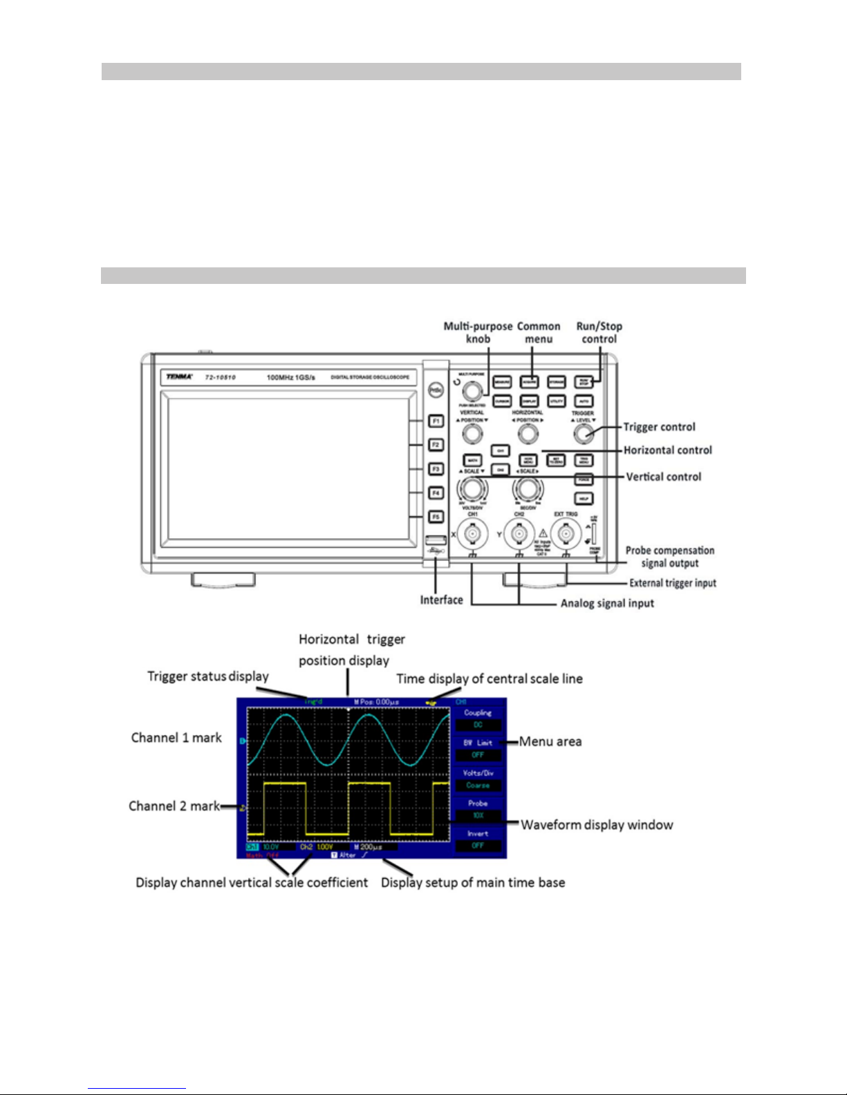
CONTROLS AND CONNECTIONS
OPERATING PARAMETERS
• The oscilloscope also has high performance index and powerful functions required
for faster measurements. Faster signals can be observed with the oscilloscope
via 500MS/s (or 1GS/s) real‐time sampling and 25GS/s (or 50GS/s) equivalent
sampling.
• Powerful trigger and analysis ability make it easier to capture and analyse
waveforms.
• Clear LCD and mathematical operating functions make it easy to use to observe
and analyse signal problems in a faster and clearer way.
4
Accessing signals
• Power on the unit then allow the self test to complete.
• Press UTILITY button then F1 and the screen will display DEFAULT SETUP.
Note: The meter has dual input channels plus one external trigger input channel.
• Press CH1 to enter channel 1 menu.
• Connect the probe to the Ch1 input.
• Set the probe attenuation switch to 10X position.
Note: The oscilloscope attenuation has to be set as well.
• Press F4 until 10X displays. This changes the vertical range multiple to ensure the
measurement result correctly reects the amplitude of the measured signal.
• Connect both probe and ground clamp to the corresponding signal terminals.
• Press AUTO and a square wave of about 3V at 1kHz is displayed for a moment.
• Press OFF then CH2 and repeat for channel 2.
OPERATION
AUTOSET WAVEFORM DISPLAY
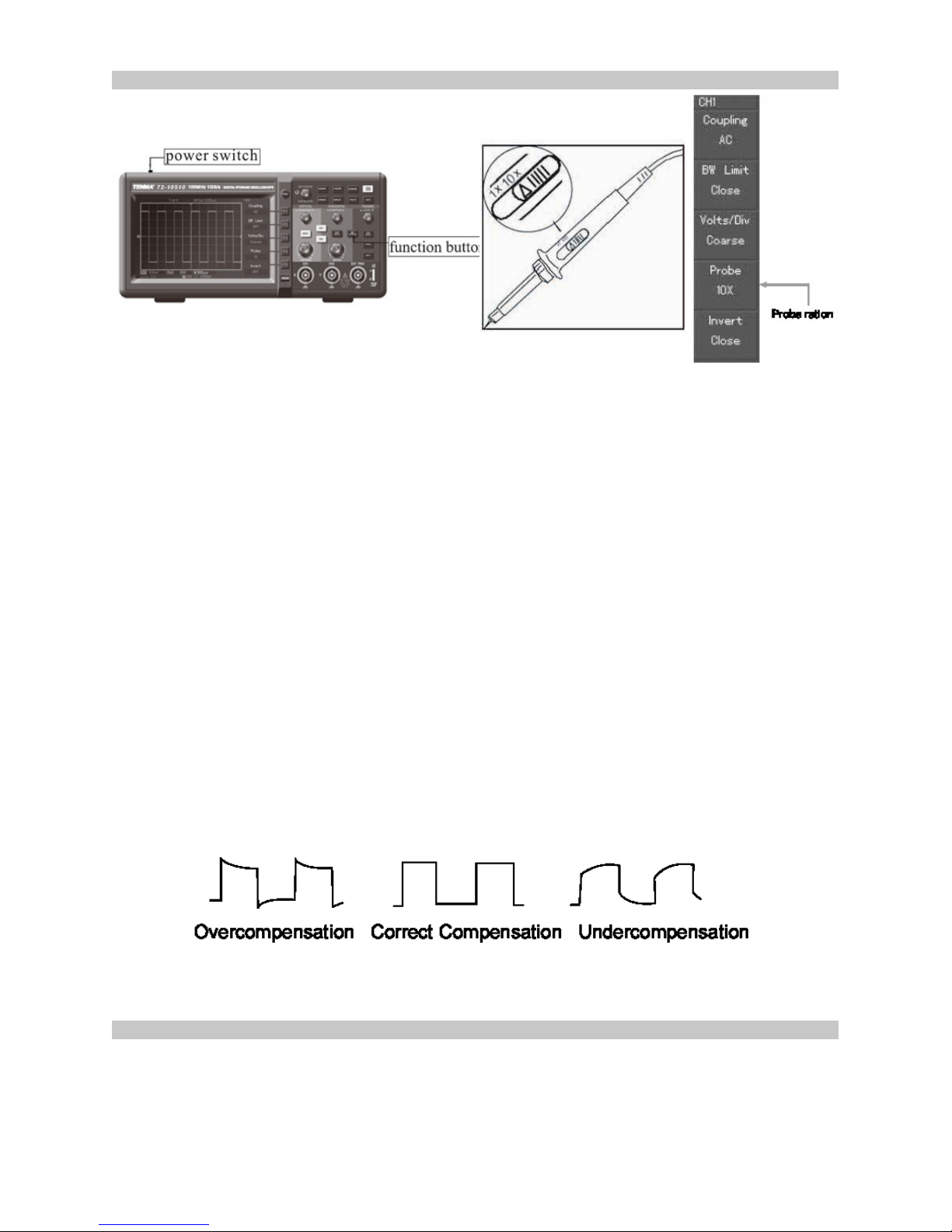
Probe compensation
• Perform this adjustment when connecting the probes to any input channel for the
rst time or errors in the measurement may result.
• Connect the probe tip to the probe compensator’s signal output connector and
connect the ground clamp to the earth wire of the probe compensator.
• Enable CH1 and press AUTO.
• Observe the shape of the displayed waveform.
• Adjust the variable capacitor on the probe with an insulated screwdriver until a
correct waveform is achieved.
• The oscilloscope features an AUTOSET function which automatically adjusts the
vertical deection factor, scanning time base and trigger mode based on the input
signal until the most appropriate waveform is displayed.
• This function only operates when the signal to be measured is 50Hz or above and
the duty ratio is larger than 1%.
5
DISPLAY SETTING CONTROLS
Using the AUTOSET function
• Connect the signal to be measured to the signal input channel.
• Press AUTO and the oscilloscope will scan the time base and trigger mode and set
the vertical deection factor. You can manually adjust further after this process to
get the optimum display.
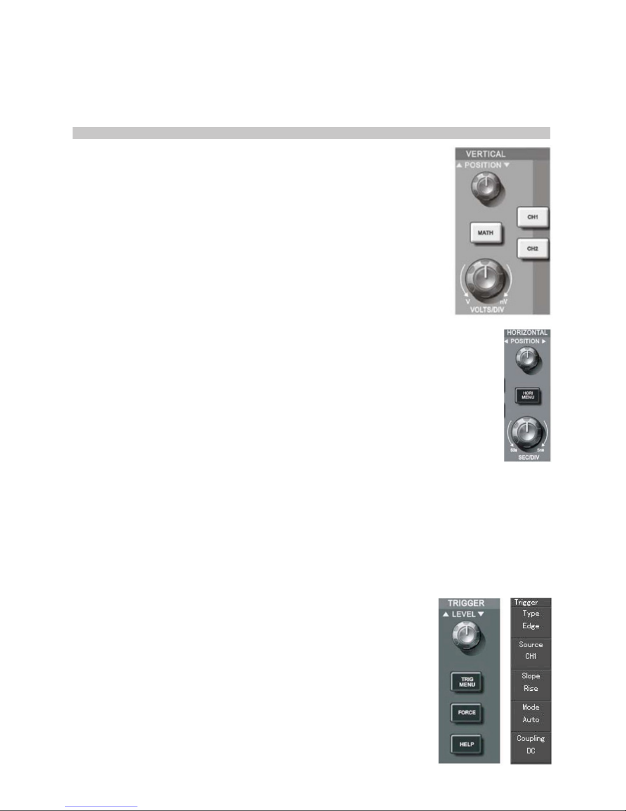
Vertical control panel
• Vertical position control centres the waveform display.
• As you adjust the position the GROUND channel indicator
moves in line with the waveform.
• Pressing SET TO ZERO resets the display to the centre point.
• Adjusting the vertical scale control adjusts the VOLT/DIV range.
The current status display changes accordingly.
• Press CH1, CH2, MATH or REFERENCE and the screen shows
the corresponding operation menu, sign, waveform and range
status information.
• Press OFF to disable the selected channel (72-2650).
Horizontal control panel
• Horizontal position control adjusts the position of the waveform window by
adjusting the trigger shift of the signal.
• The horizontal scale adjustment changes the SEC/DIV time base range
and the current status indicator will change accordingly.
• The horizontal scanning rate range is 5ns - 50ns in steps of 1-2-5-10.
Note: the horizontal scanning time base range varies between models - see
table in specication section.
• Pressing SET TO ZERO resets the display to the centre point.
Zoom display option
• Press MENU to display the ZOOM options.
• Press F3 to display further options including WINDOW EXPANSION and
HOLDOFF.
• Rotate the MULTI FUNCTION rotary control to make adjustments.
• Press F1 to quit the option and return to MAIN TIME BASE.
Trigger system
• The trigger level rotary control adjusts the trigger level. The display value changes
on the display as you make adjustment.
• Press MENU to select the trigger options.
• Press F1 and set EDGE TRIGGER
• Press F2 and set TRIGGER SOURCE to CH1
• Press F3 and set EDGE TYPE as RISING
• Press F4 and set TRIGGER MODE as AUTO
• Press F5 and set TRIGGER COUPLING as DC
• Press 50% to set trigger level at the range amplitude centre
point (trigger zero - highest sensitivity setting)
• Press COMPULSORY to generate a compulsory trigger signal
mainly used in normal and single trigger modes.
6
INSTRUMENT SETUP
Vertical system setup
• Each channel CH1 or CH2 has it’s own vertical menu. Each channel should be set
up individually.
• Press CH1 or CH2 and the system will display the operation menu for that channel.
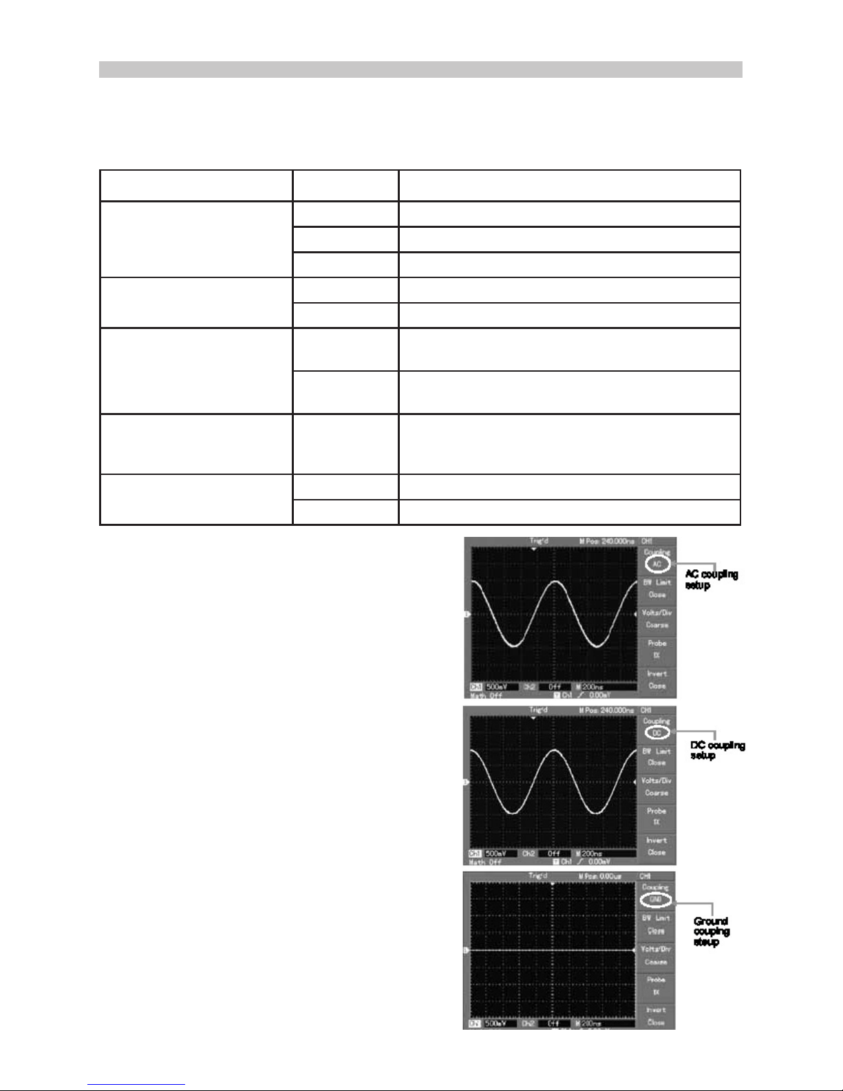
Channel coupling setup
• If for example a signal is applied to CH1
which has a sine signal that contains DC
quantities.
• Press F1 to select AC and set up as AC
coupling. Any DC quantities in the signal are
now intercepted.
• Press F1 to select DC.
• Both AC and DC quantities of the signal
being measured can now pass through.
• The waveform displays both AC and DC
quantities of the signal.
• Press F1 to select GROUND.
Both AC and DC quantities of the signal
being measured are now intercepted.
• The waveform is not displayed in this mode
but the signal remains connected to the
channel circuit.
Functions Menu Setup Notes
Coupling
AC Intercepts the DC quantities of the input signal.
DC Pass AC and DC quantities of input signal
GROUND Disconnect input signal
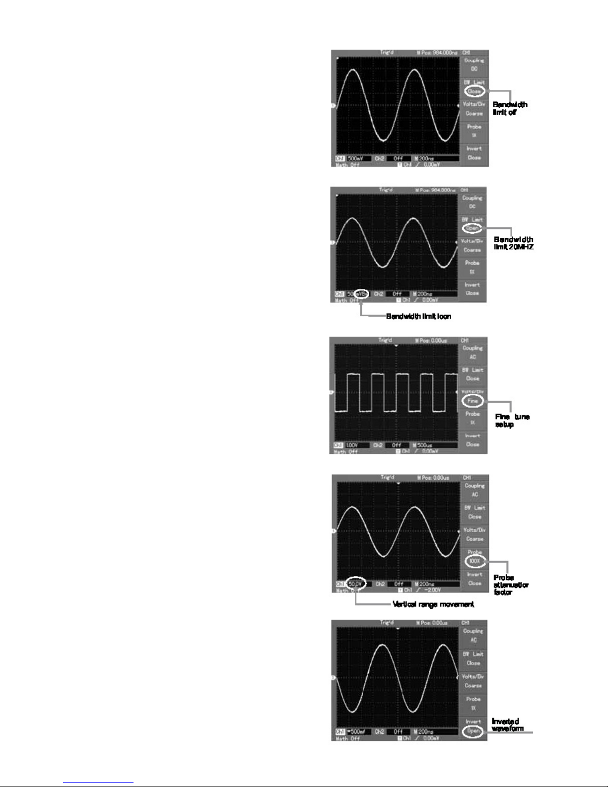
Bandwidth Limit
On Limit bandwidth to 20MHz to reduce noise display.
Off Full bandwidth
Volts / DIV
Coarse tune
Coarse tune in steps of 1-2-5 to set up the
deection factor of the vertical system.
Fine tune
Fine tune is further tuning within the coarse tune
set up to improve the vertical resolution.
Probe
1X, 10X,
100X and
1000X
Select either value based on the probe attenuation
factor to keep the vertical deection factor reading
correct.
Invert
On Waveform invert function on.
Off Normal waveform display.
7
Channel bandwidth setup
• If for example a signal is applied to CH1
which is a pulse signal that contains high
frequency oscillation.
• Press CH1 to select Channel1.
• Press F2 to set the BANDWIDTH LIMIT
OFF so it is set up as full bandwidth.
• The signal being measured can now pass
through even if it contains high frequency
quantities.
• Press F2 to set BANDWIDTH LIMIT ON
so that frequency quantities higher than
20MHz in the signal being measured will be
limited.
Probe rate setup
• To match the probe attenuation
factor setup, it is necessary to set up
the probe attenuation factor in the channel
operation menu accordingly.
• For example when the probe attenuation
factor is 10:1, set the probe attenuation
factor at 10X in the menu. This principle
applies to other values to ensure the voltage
reading is correct.
Waveform inversion setup
• The displayed signal is inverted 180
degrees with respect to the ground level.
Vertical Volts/Div adjustment setup
• The VOLTS/DIV range of the vertical
deection factor can be adjusted either in
coarse or ne tune mode.
• In COARSE TUNE the VOLTS/DIV range is
2mV/div~5V/div. Tuning is in steps of 1-2-5.
• In FINE TUNE mode the deection factor
can be adjusted in smaller steps allowing
continuous adjustment within the range
2mV/div~5V/div without interruption.
8
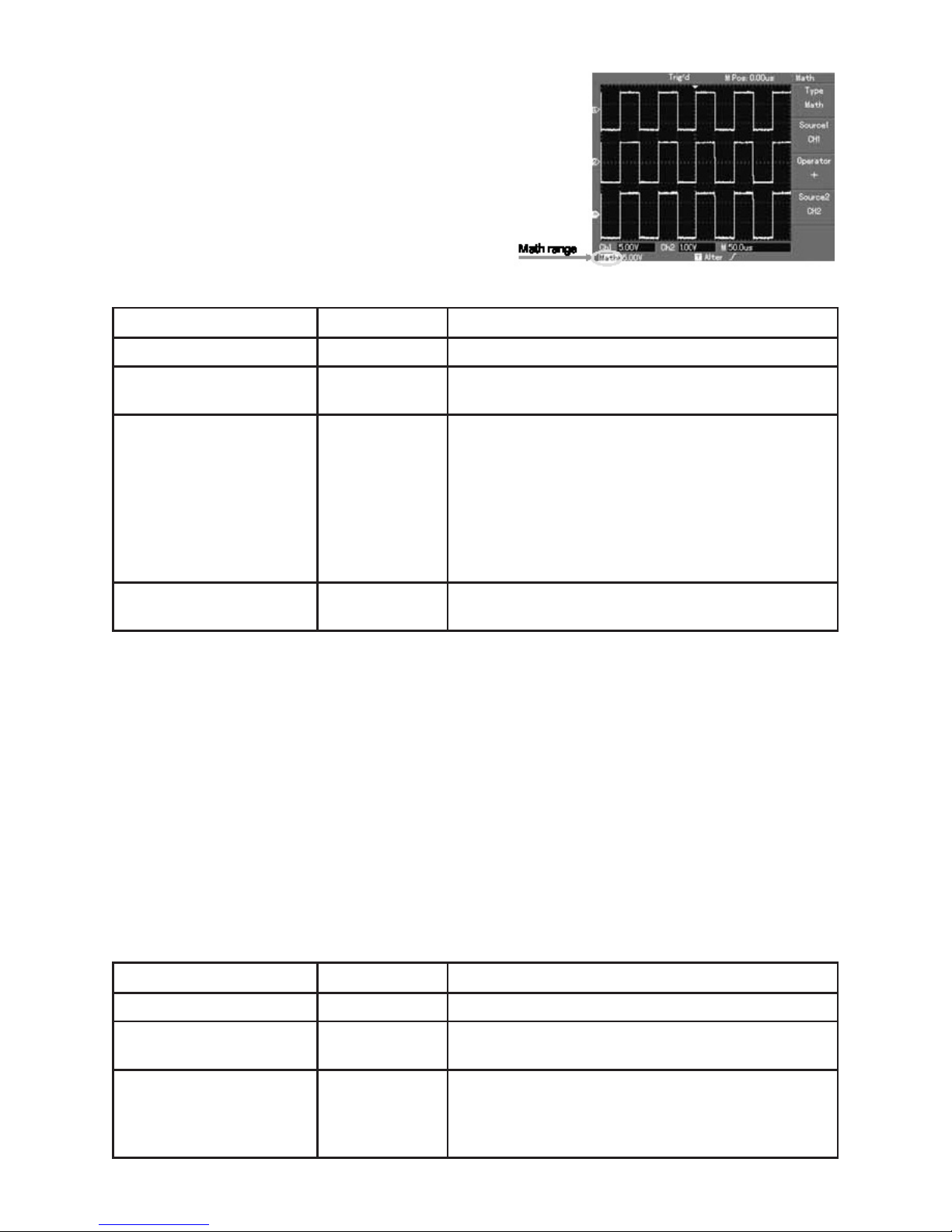
Operating Math functions
• Math functions are displays of +, -, x, ÷ and
FFT mathematical results of CH1 and CH2.
The menu options are:-
FFT spectrum analysis
• Using FFT algorithm you can convert the domain signals (YT) into frequency
domain signals.
• With FFT you can observe the following types of signals:
1. Measure the harmonic wave composition and distortion of the system.
2. Demonstrate the noise characteristics of the DC power.
3. Analyse oscillation.
• Signals with DC quantities or DC offset will cause error or offset FFT waveform
quantities. To reduce DC quantities select AC coupling.
• To reduce random noise and frequency aliasing as a result of repeated or single
pulse event, set the acquired mode of the oscilloscope to average acquisition.
Functions Menu Setup Notes
Type Math To carry out +, -, x, ÷ functions
Signal source 1 Ch1
Ch2
Set signal source 1 as CH1 waveform
Set signal source 1 as CH2 waveform
Operator +
x
÷
Signal source 1+
Signal source 2
Signal source 1-
Signal source 2
Signal source 1x
Signal source 1
Signal source 1÷
Signal source 2
Signal source 2 Ch1
Ch2
Set signal source 2 as CH1 waveform
Set signal source 2 as CH2 waveform
Functions Menu Setup Notes
Type FFT To carry out FFT algorithm functions
Signal source
Ch1
Ch2
Set CH1 as math waveform
Set CH2 as math waveform
Window
Hanning
Hamming
Blackman
Rectangle
Set Hanning window function
Set Hamming window function
Set Blackman window function
Set Rectangle window function

9
Select the FFT window
• Assuming the YT waveform is constantly repeating itself, the oscilloscope will carry
out FFT conversion of time record of a limited length. When this cycle is a whole
number, the YT waveform will have the same amplitude at the start and nish.
There is no waveform interruption.
• If the YT waveform cycle is not a whole number there will be different amplitudes
at the start and nish, resulting in transient interruption of high frequency at the
connection point. In frequency domain this is known as leakage.
• To avoid leakage multiply the original waveform by one window function to set the
value at 0 for start and nish compulsively. See the following table:
Reference waveform
• Displays of the saved reference waveforms can be set on or off in thee REF menu.
• The waveforms are saved in non-volatile memory and identied with the following
names: Ref A, Ref B.
• To display (recall) or hide the reference waveforms use the following method:
1. Press REF menu button on the front panel
2. Press REF A (reference option)
3. Select the signal source and the position of the signal source 1~10 by use of the
multi-function rotary control.
4. Press RECALL to display the waveform stored in that location.
Note: If the stored waveform is on external disk press F2 to select between DSO and
USB and select USB having inserted the drive into the USB port.
5. The recalled waveform will be displayed on the screen.
6. Press CANCEL to go back to the previous menu.
FFT Window Feature Most suitable measurement item
Rectangle
The best frequency resolution,
the worst amplitude resolution.
Basically similar to a status
without adding window.
Temporary or fast pulse. Signal level is
generally the same before and after.
Equal sine wave of very similar frequency.
There is broad-band random noise with
slow moving wave spectrum.
Hanning
Frequency resolution is better
than the rectangle window but
amplitude resolution is poorer.
Sine, cyclical and narrow-band random
noise.
Hamming
Frequency resolution is
marginally better than Hanning
window.
Temporary or fast pulse. Signal level varies
greatly before and after.
Blackman
The best amplitude resolution
and the poorest frequency
resolution.
Mainly for single frequency signals to
search for higher-order harmonic wave.
Note: FFT resolution means the quotient of the sampling and math points. When the
math point value is xed, the sampling rate should be as low as possible relative to the
FFT resolution.
• Nyquist frequency: To rebuild the original waveform, at least 2f sampling rate
should be used for waveform with a maximum frequency of f.
• This is known as Nyquist stability criterion, where f is the Nyquist frequency and 2f
is the Nyquist sampling rate.
 Loading...