Teledyne 6000B User Manual

Photometric Analyzer

OPERATING INSTRUCTIONS

Model 6000B

Photometric Analyzer

DANGER

HIGHLY TOXIC AND OR FLAMMABLE LIQUIDS OR GASES MAY BE PRESENT IN THIS MONITORING
SYSTEM.

PERSONAL PROTECTIVE EQUIPMENT MAY BE REQUIRED WHEN SERVICING THIS SYSTEM.
HAZARDOUS VOLTAGES EXIST ON CERTAIN COMPONENTS INTERNALLY WHICH MAY PERSIST

FOR A TIME EVEN AFTER THE POWER IS TURNED OFF AND DISCONNECTED.
ONLY AUTHORIZED PERSONNEL SHOULD CONDUCT MAINTENANCE AND/OR SERVICING. BEFORE

CONDUCTING ANY MAINTENANCE OR SERVICING CONSULT WITH AUTHORIZED SUPERVISOR/
MANAGER.

Teledyne Analytical Instruments

P/N M67986

11/24/04

ECO # 03-0126

i

Model 6000B

Copyright © 1999 Teledyne Analytical Instruments

All Rights Reserved. No part of this manual may be reproduced, transmitted,
transcribed, stored in a retrieval system, or translated into any other language or computer
language in whole or in part, in any form or by any means, whether it be electronic,
mechanical, magnetic, optical, manual, or otherwise, without the prior written consent of
Teledyne Analytical Instruments, 16830 Chestnut Street, City of Industry, CA 91749-

1580.

Warranty

This equipment is sold subject to the mutual agreement that it is warranted by us
free from defects of material and of construction, and that our liability shall be limited to
replacing or repairing at our factory (without charge, except for transportation), or at
customer plant at our option, any material or construction in which defects become
apparent within one year from the date of shipment, except in cases where quotations or
acknowledgements provide for a shorter period. Components manufactured by others bear
the warranty of their manufacturer. This warranty does not cover defects caused by wear,
accident, misuse, neglect or repairs other than those performed by Teledyne or an autho­rized service center. We assume no liability for direct or indirect damages of any kind and
the purchaser by the acceptance of the equipment will assume all liability for any damage
which may result from its use or misuse.

We reserve the right to employ any suitable material in the manufacture of our
apparatus, and to make any alterations in the dimensions, shape or weight of any parts, in
so far as such alterations do not adversely affect our warranty.

Important Notice

This instrument provides measurement readings to its user, and serves as a tool by
which valuable data can be gathered. The information provided by the instrument may
assist the user in eliminating potential hazards caused by his process; however, it is
essential that all personnel involved in the use of the instrument or its interface, with the
process being measured, be properly trained in the process itself, as well as all instrumen­tation related to it.

The safety of personnel is ultimately the responsibility of those who control process
conditions. While this instrument may be able to provide early warning of imminent
danger, it has no control over process conditions, and it can be misused. In particular, any
alarm or control systems installed must be tested and understood, both as to how they
operate and as to how they can be defeated. Any safeguards required such as locks, labels,
or redundancy, must be provided by the user or specifically requested of Teledyne at the
time the order is placed.

Therefore, the purchaser must be aware of the hazardous process conditions. The
purchaser is responsible for the training of personnel, for providing hazard warning
methods and instrumentation per the appropriate standards, and for ensuring that hazard
warning devices and instrumentation are maintained and operated properly.

Teledyne Analytical Instruments, the manufacturer of this instrument, cannot
accept responsibility for conditions beyond its knowledge and control. No statement
expressed or implied by this document or any information disseminated by the manufac­turer or its agents, is to be construed as a warranty of adequate safety control under the

user’s process conditions.

ii

Teledyne Analytical Instruments

Photometric Analyzer

Table of Contents

Specific Model Information................................. iv

Preface................................................................v

Part I: Control Unit.................................Part I: 1-1

Part II: Analysis Unit.............................Part II: 1-1

Appendix .........................................................A-1

Teledyne Analytical Instruments

iii

Model 6000B

iv

Teledyne Analytical Instruments

Part I: Control Unit

OPERA TING INSTRUCTIONS

Model 6000B

Photometric Analyzer

Part I: Control Unit

NEMA 4 Bulkhead Mount

Teledyne Analytical Instruments

Part I: i

Model 6000B Photometric Analyzer

Table of Contents

1 Introduction

1.1 Overview........................................................................ 1-1

1.2 Typical Applications ....................................................... 1-1

1.3 Main Features of the Analyzer ....................................... 1-1

1.4 Control Unit Inner Interface P anel .................................. 1-2

1.5 Control Unit Interface P anel........................................... 1-2

2 Installation

2.1 Unpacking the Control Unit............................................ 2-1

2.2 Mounting the Control Unit .............................................. 2-1

2.3 Electrical Connections ................................................... 2-3

2.4 Testing the System......................................................... 2-12

3 Operation

3.1 Introduction .................................................................... 3-1

3.2 Using the Data Entry and Function Buttons ................... 3-1

3.3 The System Function ..................................................... 3-4

3.3.1 Setting up an Auto-Cal........................................... 3-4

3.3.2 Pass w ord Protection.............................................. 3-6

3.3.2.1 Entering the Password...................... ... .......... 3-6

3.3.2.2 Installing or Changing the Password ............. 3-7

3.3.3 Logging Out ........................................................... 3-8

3.3.4 System Self-Diagnostic Test .................................. 3-9

3.3.5 The Model Screen ................................................. 3-10

3.3.6 Checking Linearity with Algorithm ......................... 3-10

3.3.7 Digital Flter Setup .................................................. 3-11

3.3.8 Filter or Solenoid Setup ......................................... 3-12

3.3.9 Hold/Track Setup ................................................... 3-13

3.3.11 Calibration/Hold Timer Setup................................. 3-14

3.3.12 Analog 4 to 20 mA Output Calibration.................... 3-15

3.3.12 Model..................................................................... 3-15

ii: Part I

Teledyne Analytical Instruments

Part I: Control Unit

3.3.13 Show Negative ...................................................... 3-15

3.4 The Zero and Span Functions ....................................... 3-16

3.4.1 Zero Cal ................................................................. 3-16

3.4.1.1 Auto Mode Zeroing ........................................ 3-16

3.4.1.2 Manual Mode Zeroing.................................... 3-17

3.4.1.3 Cell Failure .................................................... 3-18

3.4.2 Span Cal................................................................ 3-18

3.4.3 Offset Function....................................................... 3-20

3.4.2.1 Auto Mode Spanning ..................................... 3-19

3.4.2.2 Manual Mode Spanning................................. 3-19

3.5 The Alarms Function...................................................... 3-21

3.6 The Range Select Function ........................................... 3-23

3.6.1 Manual (Select/Define Range) Screen .................. 3-24

3.6.2 Auto Screen ........................................................... 3-24

3.6.3 Precautions............................................................ 3-26

3.7 The Analyze Function .................................................... 3-27

3.8 Programming ................................................................. 3-28

3.8.1 The Set Range Screen .......................................... 3.28

3.8.2 The Curve Algorithm Screen ................................. 3-30

3.8.2.1 Manual Mode Linearization ........................... 3-30

3.8.2.2 Auto Mode Linearization................................ 3-31

4 Maintenance

4.1 Fuse Replacement ......................................................... 4-1

4.2 System Self Diagnostic Test........................................... 4-2

4.3 Major Internal Components............................................ 4-3

A Appendix

Model 6000B Specifications .................................................. A-3

Teledyne Analytical Instruments

Part I: iii

Model 6000B Photometric Analyzer

iv: Part I

Teledyne Analytical Instruments

Photometric Analyzer Part I: Control Unit

Introduction

1.1 Overview

The Teledyne Analytical Instruments Model 6000B Control Unit,
together with a 6000B Analysis Unit, is versatile microprocessor-based
instrument.

Part I, of this manual covers the Model 6000B General Purpose NEMA
4 Bulkhead Mount Control Unit. (The Analysis Unit is covered in Part II of
this manual.) The Control Unit is for indoor/outdoor use in a nonhazardous
environment only. The Analysis Unit (or Remote Section) can be designed
for a variety of hazardous environments.

1.2 Typical Applications

A few typical applications of the Model 6000B are:

• Oil in refinery waste water condensates Streams

•CL2, HC, SO2, H2S in stack gases or Liquid Streams

• Chemical reaction monitoring

• Product Color monitoring liquids

• Petrochemical process control

• Quality assurance

• Phenol in water

• Hazardous waste incineration

• CLO2, Hypochlorite monitoring

•F2 monitoring

1.3 Main Features of the Analyzer

The Model 6000B Photometric Analyzer is sophisticated yet simple to
use. The main features of the analyzer include:

Teledyne Analytical Instruments

Part I: 1-1

1 Introduction Model 6000B

• A 2-line alphanumeric display screen, driven by microprocessor
electronics, that continuously prompts and informs the operator.

• High resolution, accurate readings of concentration from low
ppm levels through to 100%. Large, bright, meter readout.

• Versatile analysis over a wide range of applications.

• Microprocessor based electronics: 8-bit CMOS microprocessor
with 32 kB RAM and 128 kB ROM.

• Three user definable output ranges (from 0-1 ppm through
0-100 %) allow best match to users process and equipment.

• Calibration range for convenient zeroing or spanning.

• Auto Ranging allows analyzer to automatically select the proper
preset range for a given measurement. Manual override allows
the user to lock onto a specific range of interest.

• Two adjustable concentration alarms and a system failure alarm.

• Extensive self-diagnostic testing, at startup and on demand, with
continuous power-supply monitoring.

• RS-232 serial digital port for use with a computer or other digital
communication device.

• Analog outputs for concentration and range identification.
(0-1 V dc standard, and isolated 4–20 mA dc)

• Superior accuracy.

• Internal calibration (optional).

1. 4 Control Unit Inner Control Panel

The standard 6000B Control Unit is housed in a rugged NEMA 4 metal
case with all remote controls and displays accessible from the inner control
panel. See Figure 1-1. The inner control panel has a digital meter, an alpha­numeric Vacuum Fluroscent Display (VFD), and thirteen buttons for operat­ing the analyzer.

1-2: Part I

Teledyne Analytical Instruments

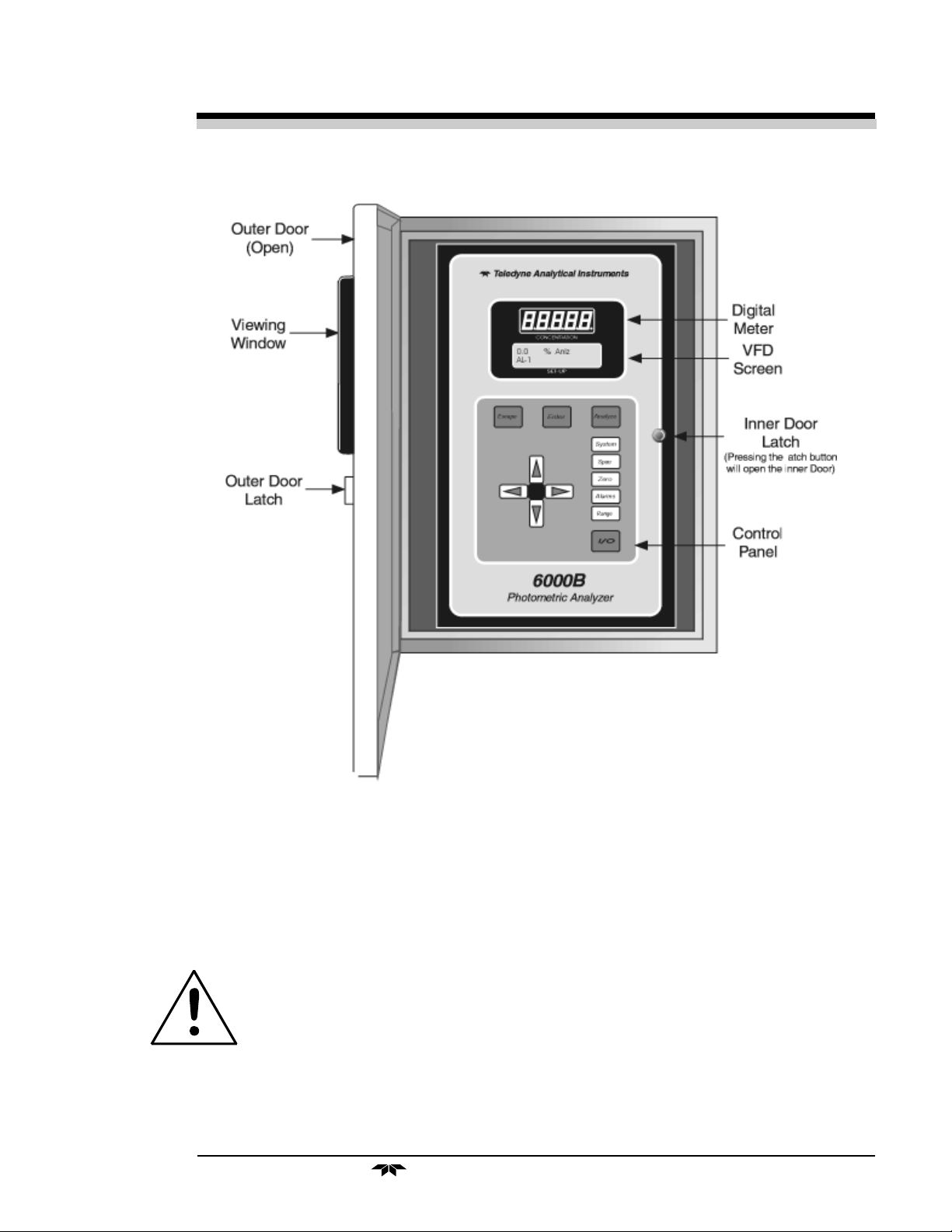
Photometric Analyzer Part I: Control Unit

Figure 1-1: Front of Unmounted Control Unit

Function Keys: Six touch-sensitive membrane switches are used to change

the specific function performed by the analyzer:

• Analyze Perform analysis for concentration content of a sample.

• System Perform system-related tasks (described in detail in chapter

3, Operation.).

• Span Span calibrate the analyzer.

• Zero Zero calibrate the analyzer.

• Alarms Set the alarm setpoints and attributes.

• Range Set up the 3 user definable ranges for the instrument.

Teledyne Analytical Instruments

Part I: 1-3

1 Introduction Model 6000B

Data Entry Keys: Six touch-sensitive membrane switches are used to
input data to the instrument via the alphanumeric VFD display:

• Left & Right Arrows Select between functions currently

displayed on the VFD screen.

• Up & Down Arrows Increment or decrement values of

functions currently displayed.

• Enter Moves VFD display on to the next screen in a series. If

none remains, returns to the Analyze screen.

• Escape Moves VFD display back to the previous screen in a

series. If none remains, returns to the Analyze screen.

Digital Meter Display: The meter display is a Light Emitting Diode
LED device that produces large, bright, 7-segment numbers that are legible
in any lighting. It is accurate across all analysis ranges. The 6000B models
produce continuous readout from 0-10,000 ppm and then switch to
continuous percent readout from 1-100 %.

Alphanumeric Interface Screen: The backlit VFD screen is an easy­to-use interface between operator and analyzer. It displays values, options,
and messages for immediate feedback to the operator.

I/O Power Button: The red I/O button switches the instrument power
between I (ON) and O (a Keep-Alive state). In the O state, the instrument’s
circuitry is operating, but there are no displays or outputs.

CAUTION: The power must be disconnected to fully

disconnect power from the instrument. When
chassis is exposed or when access door is open
and power cable is connected, use extra care to
avoid contact with live electrical circuits .

Access Door: For access to the electronics and interface panel, the front
panel swings open when the latch in the panel is pressed all the way in with
a narrow gauge tool. Accessing the main circuit board and other electronics
requires unfastening the rear panel screws and sliding the unit out of the
case.

1.5 Control Unit Interface Panel

The Control Unit interface panel, shown in Figure 1-2, contains the
electrical terminal blocks for external inputs and outputs. The input/output
functions are described briefly here and in detail in the Installation chapter of
this manual.

1-4: Part I

Teledyne Analytical Instruments

Photometric Analyzer Part I: Control Unit

Figure 1-2: Model 6000B Rear Panel

Teledyne Analytical Instruments

Part I: 1-5

1 Introduction Model 6000B

• Power Connection AC power source, 115VAC, 50/60 Hz

• Analog Outputs 0-1 V dc concentration and 0-1 V dc

range ID. Isolated 4-20 mA dc and 4-20
mA dc range ID.

• Alarm Connections 2 concentration alarms and 1 system

alarm.

• RS-232 Port Serial digital concentration signal output

and control input.

• Remote Bench Provides all electrical interconnect to the

Analysis Unit.

Remote Span/Zero Digital inputs allow external control of

analyzer calibration.

• Calibration Contact To notify external equipment that

instrument is being calibrated and
readings are not monitoring sample.

• Range ID Contacts Four separate, dedicated, range relay

contacts. Low, Medium, High, Cal.

• Network I/O Serial digital communications for local

network access. For future expansion.
Not implemented at this printing.

Note: If you require highly accurate Auto-Cal timing, use external

Auto-Cal control where possible. The internal clock in the
Model 6000B is accurate to 2-3 %. Accordingly, internally
scheduled calibrations can vary 2-3 % per day.

1-6: Part I

Teledyne Analytical Instruments

Photometric Analyzer Part I: Control Unit

Installation

Installation of Model 6000B Analyzers includes:

1. Unpacking, mounting, and interconnecting the Control Unit and
the Analysis Unit

2. Making gas connections to the system

3. Making electrical connections to the system

4. Testing the system.

This chapter covers installation of the Control Unit. (Installation of the

Analysis Unit is covered in Part II of this manual.)

2.1 Unpacking the Control Unit

The analyzer is shipped with all the materials you need to install and
prepare the system for operation. Carefully unpack the Control Unit and
inspect it for damage. Immediately report any damage to the shipping agent.

2.2 Mounting the Control Unit

The Model 6000B Control Unit is for indoor/outdoor use in a general
purpose area. This Unit is NOT for any type of hazardous environ-

ments.

Figure 2-1 is an illustration of a Model 6000B standard Control Unit
front panel and mounting brackets as shown two mounting tabs are at the top
and two at the bottom of the units frame.

Teledyne Analytical Instruments

Part I: 2-1

2 Installation Model 6000B

NPT Fittings

supplied by

customer

Viewing
W indow

0.0 % Anlz
AL -1

AC POWER IN

50/60 HZ

115V

ALARM OUTPUTS

DIGITAL INPUT SPAN ZERO

CAL. CONTACT RANGE

ID CONTACTS RS-232

SOLENOID RETURN

ANALOG OUTPUTS

NET WORK

Figure 2-1: Front Panel of the Model 6000B Control Unit

3/4" NPT

Outer Door

Latch

3/4" NPT

1" NPT

1" NPT

All operator controls are mounted on the inner control panel "door",
which is hinged on the left edge and doubles as a door to provide access to
the internal components of the instrument. The door will swing open when
the button of the latch is pressed all the way in with a narrow gauge tool
(less than 0.18 inch wide), such as a small hex wrench or screwdriver

2-2: Part I

Teledyne Analytical Instruments

Photometric Analyzer Part I: Control Unit

11.75

Figure 2-2: Required Front Door Clearance

Allow clearance for the door to open in a 90-degree arc of radius 11.75

inches. See Figure 2-2.

2.3 Electrical Connections

Figure 2-3 shows the Control Unit interface panel. Connections for
power, communications, and both digital and analog signal outputs are
described in the following paragraphs. Wire size and maximum length data
appear in the Drawings at the back of this manual.

Figure 2-3: Interface Panel of the Model 6000B Control Unit

For safe connections, ensure that no uninsulated wire extends
outside of the terminal blocks. Stripped wire ends must insert completely

into terminal blocks. No uninsulated wiring should come in contact with
fingers, tools or clothing during normal operation.

Teledyne Analytical Instruments

Part I: 2-3

2 Installation Model 6000B

Primary Input Power: The power supply in the Model 6000B will

accept a 115 Vac, 50/60 Hz power source. See Figure 2-4 for detailed
connections.

DANGER: Power is applied to the instrument's circuitry as

long as the instrument is connected to the power
source. The standby function switches power on or
off to the displays and outputs only.

115VAC

Figure 2-4: Primary Input Power Connections

Fuse Installation: The fuse holders accept 5 x 20 mm, 4.0 A, T

type (slow blow) fuses. Fuses are not installed at the factory. Be sure to
install the proper fuse as part of installation (See Fuse Replacement in
chapter 4, maintenance.)

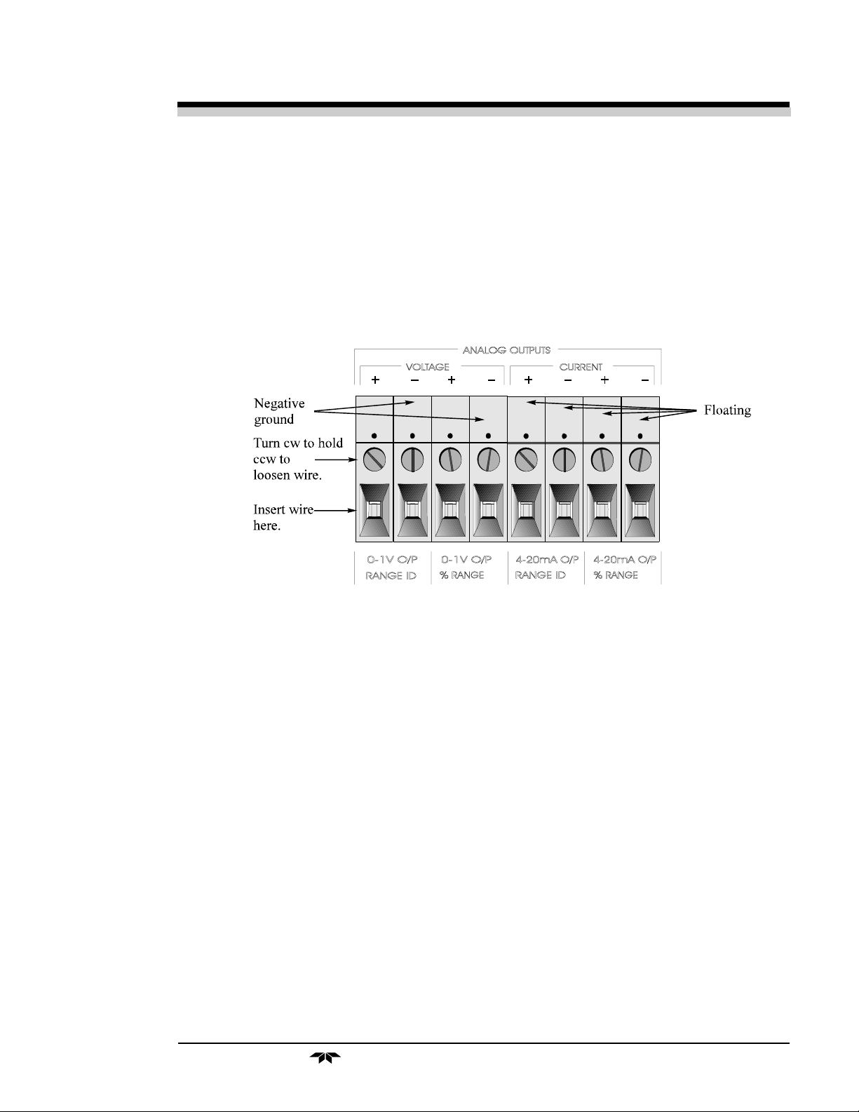
Analog Outputs: There are eight DC output signal connectors on

the ANALOG OUTPUTS terminal block. There are two connectors per
output with the polarity noted. See Figure 2-5.

The outputs are:

0–1 V dc % of Range: Voltage rises linearly with increasing sample con-

centration, from 0 V at 0% to 1 V at 100%. (Full
scale = 100% programmed range.)

0–1 V dc Range ID: 0.25 V = Low Range, 0.5 V = Medium Range,

0.75 V = High Range, 1 V = Cal Range.

2-4: Part I

Teledyne Analytical Instruments

Photometric Analyzer Part I: Control Unit

4–20 mA dc % Range: (-M Option) Current increases linearly with increas-

ing sample concentration, from 4 mA at 0% to 20
mA at full scale 100%. (Full scale = 100% of
programmed range.)

4–20 mA dc Range ID: (-M Option) 8 mA = Low Range, 12 mA = Me-

dium Range, 16 mA = High Range, 20 mA = Cal
Range.

Figure 2-5: Analog Output Connections

Examples:

The analog output signal has a voltage which depends on the sample
concentration AND the currently activated analysis range. To relate the
signal output to the actual concentration, it is necessary to know what range
the instrument is currently on, especially when the analyzer is in the
autoranging mode.

The signaloutput for concentration is linear over currently selected
analysis range. For example, if the analyzer is set on a range that was
defined as 0-10 %, then the output would be as shown in Table 2-1.

Teledyne Analytical Instruments

Part I: 2-5

2 Installation Model 6000B

Table 2-1: Analog Concentration Output-Examples

Analyte Voltage Signal Current Signal

% Output (V dc) Output (mA dc)

0 0.0 4.0
1 0.1 5.6
2 0.2 7.2
3 0.3 8.8
4 0.4 10.4
5 0.5 12.0
6 0.6 13.6
7 0.7 15.2
8 0.8 16.8
9 0.9 18.4

10 1.0 20.0

To provide an indication of the range, a second pair of analog output
terminals are used. They generate a steady preset voltage (or current when
using the current outputs) to represent a particular range. Table 2-2 gives the
range ID output for each analysis range.

Table 2-2: Analog Range ID Output - Example

Range Voltage (V) Current (mA)

LO 0.25 8
MED 0.50 12
HI 0.75 16
CAL (0-25%) 1.00 20

2-6: Part I

Teledyne Analytical Instruments

Photometric Analyzer Part I: Control Unit

N

Alarm Relays:

There are three alarm-circuit connectors on the alarm relays block
(under RELAY OUTPUTS) for making connections to internal alarm relay
contacts. Each provides a set of Form C contacts for each type of alarm.
Each has both normally open and normally closed contact connections. The
contact connections are indicated by diagrams on the rear panel. They are
capable of switching up to 3 ampers at 250 V AC into a resistive load
(Figure 2-6).

Normally closed
Normally open
Moving contact

Figure 2-6: Types of Relay Contacts

ormally open

Moving contact

The connectors are:

Threshold Alarm 1: • Can be configured as high (actuates when

concentration is above threshold), or low
(actuates when concentration is below thresh old).

• Can be configured as fail-safe or non-fail-safe.

• Can be configured as latching or nonlatching.

• Can be configured out (defeated).

Threshold Alarm 2: • Can be configured as high (actuates when concen-

tration is above threshold), or low (actuates when
concentration is below threshold).

• Can be configured as fail-safe or non-fail-safe.

• Can be configured as latching or nonlatching.

• Can be configured out (defeated).

System Alarm: Actuates when DC power supplied to circuits is

unacceptable in one or more parameters. Permanently
configured as fail-safe and latching. Cannot be de­feated. Actuates if self test fails.

Teledyne Analytical Instruments

Part I: 2-7

2 Installation Model 6000B

To reset a System Alarm during installation, discon-

nect power to the instrument and then reconnect it
Further detail can be found in chapter 3, section 4-5.

Digital Remote Cal Inputs
Remote Zero and Span Inputs: The REMOTE SPAN and RE-

MOTE ZERO inputs are on the DIGITAL INPUT terminal block. They
accept 0 V (OFF) or 24 V dc (ON) for remote control of calibration (See
Remote Calibration Protocol below.)

Zero: Floating input. 5 to 24 V input across the + and – terminals

puts the analyzer into the ZERO mode. Either side may be
grounded at the source of the signal. 0 to 1 volt across the
terminals allows ZERO mode to terminate when done. A
synchronous signal must open and close the external zero
valve appropriately. See Remote Probe Connector at end of
section 3.3. (With the -C option, the internal valves automati­cally operate synchronously).

Span: Floating input. 5 to 24 V input across the + and – terminals

puts the analyzer into the SPAN mode. Either side may be
grounded at the source of the signal. 0 to 1 volt across the
terminals allows SPAN mode to terminate when done. A
synchronous signal must open and close the external span
valve appropriately. See Remote Probe Connector at end of
section 3.3. (With the -C option, the internal valves automati­cally operate synchronously.)

Cal Contact: This relay contact is closed while analyzer is spanning

and/or zeroing. (See Remote Calibration Protocol below.)

Remote Calibration Protocol: To properly time the Digital Remote

Cal Inputs to the Model 6000B Analyzer, the customer's controller must
monitor the Cal Relay Contact.

When the contact is OPEN, the analyzer is analyzing, the Remote Cal

Inputs are being polled, and a zero or span command can be sent.

When the contact is CLOSED, the analyzer is already calibrating. It

will ignore your request to calibrate, and it will not remember that request.

Once a zero or span command is sent, and acknowledged (contact
closes), release it. If the command is continued until after the zero or span is
complete, the calibration will repeat and the Cal Relay Contact (CRC) will
close again.

For example:

2-8: Part I

Teledyne Analytical Instruments

Photometric Analyzer Part I: Control Unit

1) Test the CRC. When the CRC is open, Send a zero command
until the CRC closes (The CRC will quickly close.)

2) When the CRC closes, remove the zero command.

3) When CRC opens again, send a span command until the CRC
closes. (The CRC will quickly close.)

4) When the CRC closes, remove the span command.

When CRC opens again, zero and span are done, and the sample is

being analyzed.

Note: The Remote Bench connector (paragraph 3.3) provides signals

to ensure that the zero and span gas valves will be controlled
synchronously.

Range ID Relays: Four dedicated RANGE ID CONTACT relays .

The first three ranges are assigned to relays in ascending order—Low range
is assigned to RANGE 1 ID, Medium range is assigned to RANGE 2 ID,
and High range is assigned to RANGE 3 ID.

Network I/O: A serial digital input/output for local network protocol.

At this printing, this port is not yet functional. It is to be used in future
versions of the instrument.

RS-232 Port: The digital signal output is a standard RS-232 serial

communications port used to connect the analyzer to a computer, terminal, or
other digital device. The pinouts are listed in Table 2-3.

Table 2-3: RS-232 Signals

RS-232 Sig RS-232 Pin Purpose

DCD 1 Data Carrier Detect
RD 2 Received Data
TD 3 Transmitted Data
DTR 4 Data Terminal Ready
COM 5 Common
DSR 6 Data Set Ready
RTS 7 Request to Send
CTS 8 Clear to Send
RI 9 Ring Indicator

Teledyne Analytical Instruments

Part I: 2-9

2 Installation Model 6000B

The data sent is status information, in digital form, updated every two

seconds. Status is reported in the following order:

• The concentration in percent

• The range is use (HI< MED< LO)

• The span of the range 0-100%, etc)

• Which alarm - if any - are disabled (AL-x DISABLED)

• Which alarms - if any - are tripped (AL-x ON)

Each status output is followed by a carriage return and line feed.

Three input functions using RS-232 have been implemented to date.

They are described in Table 2-4.

Table 2-4: Commands via RS-232 Input

Command Description
as<enter> Immediately starts an autospan.
az<enter> Immediately starts an autozero.
st<enter> Toggling input. Stops/Starts any status message output

from the RS-232, Until st<enter> is sent again.

The RS-232 protocol allows some flexibility in its implementation.

Table 2-5 lists certain RS-232 values that are required by the 6110B.

Table 2-5: Required RS-232 Options

Parameter Setting

Baud 2400

Byte 8 bits

Parity none

Stop Bits 1

Message Interval 2 seconds

Remote Bench and Solenoid Valves: The 6000B is a single-chassis

instrument. However, the REMOTE BENCH and SOLENOID RETURN
connectors are provided on the interface PCB. The Remote Bench is wired
at the factory as well as any optional solenoid valves included in the system.

2-10: Part I

Teledyne Analytical Instruments

Photometric Analyzer Part I: Control Unit

2.4 Testing the System

After The Control Unit and the Analysis Unit are both installed and

interconnected, and the system gas and electrical connections are complete,
the system is ready to test. Before plugging either of the units into their
respective power sources:

• Check the integrity and accuracy of the gas connections. Make
sure there are no leaks.

• Check the integrity and accuracy of all electrical connections.
Make sure there are no exposed conductors

• Check that sample pressure typically between 0 and 30 psig,
according to the requirements of your process.

Power up the system, and test it by performing the following operation:

1. Repeat the Self-Diagnostic Test as.

Teledyne Analytical Instruments

Part I: 2-11

2 Installation Model 6000B

2-12: Part I

Teledyne Analytical Instruments

Photometric Analyzer Operation 3

Operation

3.1 Introduction

Although the Model 6000B is usually programmed to your application at

the factory, it can be further configured at the operator level, or even, cautious-
ly, reprogrammed. Depending on the specifics of the application, this might
include all or a subset of the following procedures:

• Setting system parameters:

• Establish a security password, if desired, requiring Operator
to log in (secure in safe file for referrence).

• Establish and start an automatic calibration cycle, if desired.

• Routine Operation:

• Calibrate the instrument.

• Choose autoranging or select a fixed range of analysis.

• Set alarm setpoints, and modes of alarm operation (latching,
fail-safe, etc).

• Program/Reprogram the analyzer:

• Define new applications.

• Linearize your ranges.

If you choose not to use password protection, the default password is

automatically displayed on the password screen when you start up, and you
simply press Enter for access to all functions of the analyzer.

3.2 Using the Data Entry and Function
Buttons

Data Entry Buttons: The < > buttons select options from the menu

currently being displayed on the VFD screen. The selected option blinks.

When the selected option includes a modifiable item, the

can be used to increment or decrement that modifiable item.

Teledyne Analytical Instruments

ΔΔ

Δ∇ arrow buttons

ΔΔ

Part I 3-1

3 Operation Model 6000

The Enter button is used to accept any new entries on the VFD screen.

The Escape button is used to abort any new entries on the VFD screen that are
not yet accepted by use of the Enter button.

Figure 4-1 shows the hierarchy of functions available to the operator via the

function buttons. The six function buttons on the analyzer are:

• Analyze. This is the normal operating mode. The analyzer

monitors the thermal conductivity of the sample, displays the
percent or parts-per-million of target gas or contamination, and
warns of any alarm conditions.

• System. The system function consists of nine subfunctions.
Four of these are for ordinary setup and operation:

• Setup an Auto-Cal

• Assign Passwords

• Log out to secure system

• Initiate a Self-Test

Three of the subfunctions do auxiliary tasks:

• Checking model and software version

• Adjust electronic filter of the signal

• Display more subfunctions

• Display negative readings

Two of these are for programming/reprogramming the analyzer:

• Define gas applications and ranges (Refer to programming
section, or contact factory.)

• Use the Curve Algorithm to linearize output. (Refer to
programming section, or contact factory.)

• Zero. Used to set up a zero calibration.

• Span. Used to set up a span calibration.

• Alarms. Used to set the alarm setpoints and determine whether

each alarm will be active or defeated, HI or LO acting, latching,
and/or fail-safe.

• Range. Used to set up three analysis ranges that can be

switched automatically with autoranging or used as individual
fixed ranges.

Any function can be selected at any time by pressing the appropriate button
(unless password restrictions apply). The order as presented in this manual is
appropriate for an initial setup.

Each of these functions is described in greater detail in the following proce­dures. The VFD screen text that accompanies each operation is reproduced, at

3-2 Part I

Teledyne Analytical Instruments

Photometric Analyzer Operation 3

System

Dig_filt

SELF-TEST

PWD

LOGOUT

MORE

AUTOCAL

FILSOL

TRACK or

HOLD

CAL-HOLD

TIMER

Set Digital

Filter

Self-Test in

Progress

Enter

Password

Secure System

setup not allowed

Span/Zero status

and <>setup

Span/Zero

Solenoid or Filter

Set track or

hold output

Set cal. hold and

sample hold

timer

Self-Test

Results

Change
Yes/No

Span/Zero timing

and on/off

Enter

Enter

Change

Password

Enter

Verify

Password

Enter

MORE

ALGORITHM

APPLICATION

OUTPUT:

4 or 20 MA

MORE

MODEL

SHOW.NEG

Select range

Select range

Set current

output

Display

Model/Version

Show
Negative
Reading

Display gas use

and range

Define

Application/

Range

Enter

Enter

Select

Verify/Setup

Enter

Verify data

Points

Auto/Manual

linear Cal.

Enter

Enter

Input/Output

Enter Span

gas value

Figure 3-1: Hierarchy of System Functions and Subfunctions

Enter

Enter

Teledyne Analytical Instruments

Part I 3-3

3 Operation Model 6000

the appropriate point in the procedure, in a Monospaced type style. Push­button names are printed in Oblique type.

3.3 The System Function

The subfuctions of the System function are described below. Specific

procedures for their use follow the descriptions:

• Dig_Filt: Adjust how much digital filtering should be on the

signal

• SELF-TEST: Performs a self-diagnostic test to check the

integrity of the power supplies, outputs, detector signal and
preamplifier.

• PWD: Login security system for accessing to the setup functions.

• LOGOUT: Prevents an unauthorized tampering with analyzer

settings.

• AUTOCAL: Set the automatic calibrated timer schedule for Zero

and Span cycling.

• FILSOL: Select Span/Zero flag (filter) or Span/Zero solenoid

valve for calibration method.

• TRACK: Set the system reading to be held or followed by the

concentration “gas or filter” during calibration.

• CAL-HOLD-TIMER: Set the timing for calibration holding and

timing for the sample reading after return to analyze mode.

• ALGORITHM: Linearize the output for nonlinear characteristic.

• APPLICATION: Used to define the analysis ranges and

application (gas used).

• MODEL: Displays model number and software version.

• OUTPUT: 4-20 MA: Adjust 4 and 20 mA output.

• SHOW_NEG: Whether to display negative readings or not; affects

analog output too. No negative readings is the default.

3.3.1 Setting up an AUTO-CAL

When proper automatic valving is connected, the Analyzer can cycle itself

through a sequence of steps that automatically zero and span the instrument.

3-4 Part I

Teledyne Analytical Instruments

Photometric Analyzer Operation 3

Note: Before setting up an AUTO-CAL, be sure you understand the

Zero and Span functions as described in section 4.4, and
follow the precautions given there.

Note: If you require highly accurate AUTO-CAL timing, use external

AUTO-CAL control where possible. The internal clock in the
Model 6000B is accurate to 2-3 %. Accordingly, internally
scheduled calibrations can vary 2-3 % per day.

To setup an Auto–Cal cycle:
Choose System from the Function buttons. TheVFD will display five

subfunctions.

DIG_FILT SELF—TEST
PWD LOGOUT MORE

Select MORE and press the Enter Key

AUTOCAL FILSOL HOLD
CAL-HOLD-TIMER MORE

Use < > arrows to blink AUTO—CAL, and press Enter. A new screen

for ZERO/SPAN set appears.

ZERO in Ød Øh off
SPAN in Ød Øh off

Press < > arrows to blink ZERO (or SPAN), then press Enter again.

(You won’t be able to set OFF to ON if a zero interval is entered.) A Span
Every ... (or Zero Every ...) screen appears.

Zero schedule: OFF
Day: Ød Hour: Øh

ΔΔ

Use

Δ∇ arrows to set an interval value, then use < > arrows to move to the

ΔΔ

start-time value. Use

ΔΔ

Δ∇ arrows to set a start-time value.

ΔΔ

To turn ON the SPAN and/or ZERO cycles (to activate AUTO–CAL):
Press System again, choose AUTO–CAL, and press Enter again. When the
ZERO/SPAN values screen appears, use the < > arrows to blink the ZERO
(or SPAN) and press Enter to go to the next screen. Use < > to select OFF/
ON field. Use

ΔΔ

Δ∇ arrows to set the OFF/ON field to ON. You can now turn

ΔΔ

these fields ON because there is a nonzero span interval defined.

If instrument is turned off, the next time the instrument is powered, the
instrument will automatically perform a calibration cycle after 3 minutes of
entering the sample mode if AUTOCAL functions were on prior to shut down.

Teledyne Analytical Instruments

Part I 3-5

3 Operation Model 6000

3.3.2 Password Protection

Before a unique password is assigned, the system assigns TAI by default.

This password will be displayed automatically. The operator just presses the
Enter key to be allowed total access to the instrument’s features.

If a password is assigned, then setting the following system parameters can

be done only after the password is entered: alarm setpoints, assigning a new
password, range/application selections, and curve algorithm linearization.
(APPLICATION and ALGORITHM are covered in the programming section.)
However, the instrument can still be used for analysis or for initiating a self-test
without entering the password. To defeat security the password must be
changed back to TAI.

NOTE: If you use password security, it is advisable to keep a copy of

the password in a separate, safe location.

3.3.2.1 Entering the Password

To install a new password or change a previously installed password, you

must key in and ENTER the old password first. If the default password is in
effect, pressing the ENTER button will enter the default TAI password for you.

Press System to enter the System mode.

DIG_FILT AUTO—CAL
PWD LOGOUT MORE

Use the < > arrow keys to scroll the blinking over to PWD, and press

Enter to select the password function. Either the default TAI password or AAA
place holders for an existing password will appear on screen depending on
whether or not a password has been previously installed.

Enter password:
T A I

or

Enter password:
A A A

The screen prompts you to enter the current password. If you are not using

password protection, press Enter to accept TAI as the default password. If a
password has been previously installed, enter the password using the < > arrow
keys to scroll back and forth between letters, and the

ΔΔ

Δ∇ arrow keys to change

ΔΔ

the letters to the proper password. Press Enter to enter the password.

3-6 Part I

Teledyne Analytical Instruments

Photometric Analyzer Operation 3

In a few seconds, you will be given the opportunity to change this pass­word or keep it and go on.

Change Password?
<ENT>=Yes <ESC>=No

Press Escape to move on, or proceed as in Changing the Password,
below.

3.3.2.2 Installing or Changing the Password

If you want to install a password, or change an existing password, proceed
as above in Entering the Password. When you are given the opportunity to
change the password:

Change Password?
<ENT>=Yes <ESC>=No

Press Enter to change the password (either the default TAI or the previ-
ously assigned password), or press Escape to keep the existing password and
move on.

If you chose Enter to change the password, the password assignment
screen appears.

Select new password
T A I

Enter the password using the < > arrow keys to move back and forth
between the existing password letters, and the

ΔΔ

Δ∇ arrow keys to change the

ΔΔ

letters to the new password. The full set of 94 characters available for password
use are shown in the table below.

Characters Available for Password Definition:

ABCDEFGHIJ
KLMNOPQRST
UVWXYZ[¥]^
_`abcdefgh
ijklmnopqr
stuvwxyz{|
} → !"#$%&'(
)*+'-./012
3456789:;<
=>?@

When you have finished typing the new password, press Enter. A verifica­tion screen appears. The screen will prompt you to retype your password for
verification.

Teledyne Analytical Instruments

Part I 3-7

3 Operation Model 6000

Enter PWD To Verify:
A A A

Use the arrow keys to retype your password and press Enter when
finished. Your password will be stored in the microprocessor and the system will
immediately switch to the Analyze screen, and you now have access to all
instrument functions.

If all alarms are defeated, the Analyze screen appears as:

1.95 ppm SO
nR1: Ø — 1Ø Anlz

2

If an alarm is tripped, the second line will change to show which alarm it is:

1.95 ppm SO
AL—1

NOTE:If you log off the system using the LOGOUT function in the

system menu, you will now be required to re-enter the pass­word to gain access to Alarm, and Range functions.

2

3.3.3 Logging Out

The LOGOUT function provides a convenient means of leaving the
analyzer in a password protected mode without having to shut the instrument off.
By entering LOGOUT, you effectively log off the instrument leaving the system
protected against use until the password is reentered. To log out, press the
System button to enter the System function.

DIG_FILT SELF-TEST
PWD LOGOUT MORE

Use the < > arrow keys to position the blinking over the LOGOUT function,
and press Enter to Log out. The screen will display the message:

Protected until
password entered

3.3.4 System Self-Diagnostic Test

The Model 6000B has a built-in self-diagnostic testing routine. Pre-pro­grammed signals are sent through the power supply, output board, preamp
board and sensor circuit. The return signal is analyzed, and at the end of the test
the status of each function is displayed on the screen, either as OK or as a
number between 1 and 1024. (See System Self Diagnostic Test in chapter 4
for number code.) If any of the functions fails, the System Alarm is tripped.

3-8 Part I

Teledyne Analytical Instruments

Photometric Analyzer Operation 3

Note: The sensor will always show failed unless Zero gas is present

in the sampling cell at the time of the SELF-TEST.

The self diagnostics are run automatically by the analyzer whenever the
instrument is turned on, but the test can also be run by the operator at will. To
initiate a self diagnostic test during operation:

Press the System button to start the System function.

DIG_FILT SELF-TEST
PWD LOGOUT MORE

Use the < > arrow keys again to move the blinking to the SELF–TEST
and press Enter. The screen will follow the running of the diagnostic.

RUNNING DIAGNOSTIC
Testing Preamp — Cell

When the testing is complete, the results are displayed.

Power: OK Analog: OK
Cell: 2 Preamp: 3

The module is functioning properly if it is followed by OK. A number
indicates a problem in a specific area of the instrument. Refer to Chapter 5
Maintenance and Troubleshooting for number-code information. The results
screen alternates for a time with:

Press Any Key
To Continue...

Then the analyzer returns to the initial System screen.

3.3.5 The Model Screen

Move the < > arrow key to MORE and press Enter. With MODEL
blinking, press Enter. The screen displays the manufacturer, model, and soft­ware version information.

3.3.6 Checking Linearity with ALGORITHM

From the System Function screen, select ALGORITHM, and press
Enter.

sel rng to set algo:
—> Ø1 Ø2 Ø3 <—

Teledyne Analytical Instruments

Part I 3-9

3 Operation Model 6000

Use the < > keys to select the range: 01, 02, or 03. Then press Enter.

Gas Use: SO2
Range: Ø — 10%

Press Enter again.

Algorithm setup:
VERIFY SET UP

Select and Enter VERIFY to check whether the linearization has been

accomplished satisfactorily.

Dpt INPUT OUTPUT
Ø Ø.ØØ Ø.ØØ

The leftmost digit (under Dpt) is the number of the data point being moni-

tored. Use the Δ∇ keys to select the successive points.

The INPUT value is the input to the linearizer. It is the simulated output of

the analyzer. You do not need to actually flow gas.

The OUTPUT value is the output of the linearizer. It should be the ACTU-

AL concentration of the span gas being simulated.

If the OUTPUT value shown is not correct, the linearization must be
corrected. Press ESCAPE to return to the previous screen. Select and Enter
SET UP to Calibration Mode screen. (set-up will not work without a PC being
connected to the analyzer)

Select algorithm
mode : AUTO

There are two ways to linearize: AUTO and MANUAL: The auto mode
requires as many calibration gases as there will be correction points along the
curve. The user decides on the number of points, based on the precision re­quired.

The manual mode only requires entering the values for each correction
point into the microprocessor via the front panel buttons. Again, the number of
points required is determined by the user.

3.3.7 Digital Filter Setup

The 6000B has the option of decreasing or increasing the amount filtering
on the signal. This feature enhances the basic filtering done by the analog circuits
by setting the amount of digital filtering effected by the microprocessing. To
access the digital filter setup, you must:

1. Press the System key to start the System function

3-10 Part I

Teledyne Analytical Instruments

Photometric Analyzer Operation 3

DIG_FILT SELF-TEST
PWD LOGOUT MORE

2. DIG_FILT will flash, press the ENTER key,

Weight of digital
Filter: 9

3. The number on the second row will flash and can be set by
using the Up or Down arrow keys.

The settings go from zero, no digital filtering, to 10, maximum digital filter­ing. The default setting is 8 and that should suffice for most applications. In
some applications where speeding the response time with some trade off in noise
is of value, the operator could decrease the number of the digital filter. In
applications where the signal is noisy, the operator could switch to a higher
number; the response time is slowed down though.

90% response time on the different settings to a step input is shown below.
This response time does not include the contributions of the bench sampling
system and the preamplifier near the detector.

Setting 90% Response time

(seconds)

0 4.5

1 4.5

2 5.0

3 5.0

4 5.5

5 7.0

6 9.0

7 14.0

8 25.0

9 46.0

10 90.0

At a setting of “zero”, the response time is purely set by the electronics to

4.5 seconds. The numbers above can and will change depending on application
and they merely serve to illustrate the effect of the digital filter.

Teledyne Analytical Instruments

Part I 3-11

3 Operation Model 6000

3.3.8 Filter or Solenoid Setup

The 6000B can be spanned or zeroed by calibration gases or by the optical
filters. The proper calibration method should be set at the factory. To access
the Filter or Solenoid Flags, you must:

1. Press the System key to start the System function:

DIG_FILT SELF-TEST
PWD LOGOUT MORE

2. Using the Right or Left arrow keys, select MORE and press Enter. The

second System screen appears:

AUTOCAL FILSOL TRACK
CAL-HOLD-TIMER MORE

3. Select FILSOL using the Right or Left arrow keys and press Enter to

start the method of calibration function.

Set fil/sol for cal
Span: FIL Zero: SOL

There are two flag options: zero and/or span flags are choosen at time of
purchase, one for Zero calibration and the other for Span located in the Detector
housing. To move between the Zero and the Span flags, use the Right or Left
arrow keys. FIL means that a filter will do this particular calibration. SOL
means that the signal to activate a gas solenoid is enabled. To toggle between
the SOL and FIL options, use the Up and Down arrow keys.

The connections to drive the filter and the solenoid are found on a strip
terminal located on the interface board. The connections are described in
section 5-6 of the maintenance section of the manual.

3.3.9 Hold/Track Setup

The 6000B has ability to disable the analog outputs and freeze the display
while undergoing a scheduled or remote calibration. The 6000B will track

changes in the concentration if calibration is started through the front
panel. To setup this feature, the operator must:

1. Press the System key to start the System function:

2. Using the Right or Left arrow keys, select MORE and press

3-12 Part I

DIG_FILT SELF-TEST
PWD LOGOUT MORE

Enter. The Second System screen appears:

Teledyne Analytical Instruments

Photometric Analyzer Operation 3

AUTOCAL FILSOL TRACK
CAL-HOLDER-TIMER MORE

or

AUTOCAL FILSOL HOLD
CAL-HOLD-TIMER MORE

3. The option on the right of the first row can be set to TRACK or
HOLD by using the UP or Down keys. By selecting the TRACK option, the
analog outputs are enabled and with the display will track the concentration
changes while the instrument is undergoing scheduled or remote calibration
(either zero or span). By selecting the HOLD option, the analog outputs and
display are disabled and will not track the concentration changes while the
instrument is undergoing scheduled or remote calibration (either zero or span).
In the HOLD option, the analog outputs and display will freeze on the last
reading before entering calibration.

The analog outputs are both 0 to 1 volt outputs and both 4 to 20 mA

outputs.

3.3.10 Calibration/Hold Timer Setup

This Calibration Timer lets the operator adjust the time thee instrument
purges the calibration gas prior to actually start the calibration computations.
The Sample timer lets the operator adjust the time the instrument purges sample
gas after finishing a calibration before it lets the analog outputs and display track
the change in concentration.

This function and the TRACK/HOLD feature will prevent false alarms
while performing remote or autoscheduled calibrations. These functions are not
applicable if the calibration is initiated through the front panel. To enter the
Calibration/Hold Timer function, you must:

1. Press the System key to start the System function:

DIG_FILT SELF-TEST
PWD LOGOUT MORE

2. Using the Right or Left arrow keys, select MORE and press

Enter: The Second System screen appears:

AUTOCAL FILSOL TRACK
CAL-HOLD-TIMER MORE

or

Teledyne Analytical Instruments

Part I 3-13

3 Operation Model 6000

AUTOCAL FILSOL HOLD
CAL-HOLD-TIMER MORE

3. Select with the Right or Left keys CAL-HOLD-TIMER, and

press the Enter key to access this function menu:

Calbrt hold: 3 min

Sample hold: 1 min

The calibration hold time is set on the first row, while the sample hold
time is set on the second row. To select one or the other, use the Right or
Left keys. To modify the time of either timer, use the Up or Down keys.
The time is in the minutes.

3.3.11 Analog 4 to 20 mA Output Calibration

This function will let the operator calibrate the 4 to 20 mA analog output to
match the display reading. A DMM configure as a DC ammeter is needed. The
DMM should be connected across the output terminals of the 4 to 20 mA output
to monitor the output current. To enter the 4 to 20 mA output adjust function,
you must:

1. Press the System key to start the System function:

DIG_FILT SELF-TEST
PWD LOGOUT MORE

2. Using the Right or Left arrow keys, select MORE and press

Enter. The second System screen appears:

AUTOCAL FILSOL TRACK
CAL-HOLD-TIMER MORE

or

AUTOCAL FILSOL HOLD
CAL-HOLD-TIMER MORE

3. Using the Right or the Left arrow keys, select MORE and

press Enter. The third System screen appears:

ALGORITHM APPLICATION
MODEL OUTPUT: 4 MA

ALGORITHM APPLICATION
MODEL OUTPUT: 20 MA

or

3-14 Part I

Teledyne Analytical Instruments

Photometric Analyzer Operation 3

OUTPUT: 4 MA and OUTPUT: 20 MA can be toggled by moving on
that field and pressing the Up or Down key. 4 mA output should be calibrat­ed first and 20 mA output afterwards.

4. Select OUTPUT: 4 MA and press the Enter key

Use UP/DOWN arrow to

Adjust 4 ma: 250

The number on the second row is the setpoint of the 4 mA output. It is
analogous to a potentiometer wiper. The number can be set anywhere from 0
to 500. The default is 250, in the middle. At the default setting, the output
should be very close to 4 mA. If not, slowly adjust the number using the Up or
the Down keys until DMM reads 4.00 mA. Press the Enter key when done.

5. Now select OUTPUT: 20 MA and press the Enter key. A
screen similar to the one above will appear and the DMM should read close to
20 mA. If not, slowly adjust the number using the Up or Down key until DMM
reads 20.0 mA. Press the Enter key when done.

The range of adjustment is approximately +/- 10% of scale (+/- 1.6 ma).
Since the 4 to 20 mA output is tied to the 0 to 1 volt output, this function can be
used to calibrate the 0 to 1 volt output, if the 4 to 20 mA output is not used. By
using a digital Volt meter on the 0-1 Volt output.

3.3.12 Model

This selection in the System menu flashes for a few seconds the model
number and the software version installed in this instrument.

3.3.13 Show Negative

The analyzer defaults to not to show negative readings on the analyze mode
only. This affects the analog outputs too by pressing the UP or DOWN key, the
analyzer can be set to display negative readings, on the SHOW_NEG field of
the system menu.

3.4 The Zero and Span Functions

The Model 6000B can have as many as three analysis ranges plus a
special calibration range (Cal Range). Calibrating any one of the ranges will
automatically calibrate the other ranges.

CAUTION: Always allow 4-5 hours warm-up time before calibrat-

ing, if your analyzer has been disconnected from its

Teledyne Analytical Instruments

Part I 3-15

3 Operation Model 6000

power source. This does not apply if the analyzer
was plugged in but was in STANDBY.

The analyzer is calibrated using zero, and span gases.

Note: Shut off the gas pressure before connecting it to the analyzer,

and be sure to limit pressure to 40 psig or less when turning it
back on.

Readjust the gas pressure into the analyzer until the flowrate through the
Sample Cell settles between 50 to 200 cc/min (approximately 0.1 to 0.4
SCFH).

Note: Always keep the calibration gas flow as close to the flowrate of

the sample gas as possible

3.4.1 Zero Cal

The Zero button on the front panel is used to enter the zero calibration
function. Zero calibration can be performed in either the automatic or manual
mode.

Make sure the zero gas is flowing to the instrument. If you get a CELL
CANNOT BE BALANCED message while zeroing skip to section 4.4.1.3.

3.4.1.1 Auto Mode Zeroing

Observe the precautions in sections 4.4 and 4.4.1, above. Press Zero to
enter the zero function mode. The screen allows you to select whether the zero
calibration is to be performed automatically or manually. Use the Δ∇ arrow
keys to toggle between AUTO and MAN zero settling. Stop when AUTO
appears, blinking, on the display.

Select zero
mode: AUTO

Press Enter to begin zeroing.

####.## % SO2
Slope=#.### C—Zero

The beginning zero level is shown in the upper left corner of the display. As
the zero reading settles, the screen displays and updates information on Slope=
in percent/second (unless the Slope starts within the acceptable zero range and
does not need to settle further). The system first does a coarse zero, shown in

3-16 Part I

Teledyne Analytical Instruments

Photometric Analyzer Operation 3

the lower right corner of the screen as
zero, and displays

F—Zero

, for 3 min.

C—Zero

, for 3 min, and then does a fine

Then, and whenever Slope is less than 0.01 for at least 3 min, instead of

Slope you will see a countdown: 9 Left, 8 Left, and so fourth. These are
software steps in the zeroing process that the system must complete, AFTER
settling, before it can go back to Analyze. Software zero is indicated by S–
Zero in the lower right corner.

####.## % SO2
4 Left=#.### S—Zero

The zeroing process will automatically conclude when the output is within

the acceptable range for a good zero. Then the analyzer automatically returns to
the Analyze mode.

3.4.1.2 Manual Mode Zeroing

Press Zero to enter the Zero function. The screen that appears allows you

to select between automatic or manual zero calibration. Use the Δ∇ keys to
toggle between AUTO and MAN zero settling. Stop when MANUAL appears,
blinking, on the display.

Select zero
mode: MANUAL

Press Enter to begin the zero calibration. After a few seconds the first of

three zeroing screens appears. The number in the upper left hand corner is the
first-stage zero offset. The microprocessor samples the output at a predeter­mined rate.

####.## % SO2
Zero adj:2048 C—Zero

The analyzer goes through C–Zero, F–Zero, and S–Zero. During C–Zero

and F–Zero, use the

ΔΔ

Δ∇ keys to adjust displayed Zero adj: value as close as

ΔΔ

possible to zero. Then, press Enter.

S–Zero starts. During S–Zero, the Microcontroller takes control as in Auto

Mode Zeroing, above. It calculates the differences between successive sam­plings and displays the rate of change as Slope= a value in parts per million per
second (ppm/s).

####.## % SO2
Slope=#.### S—Zero

Teledyne Analytical Instruments

Part I 3-17

3 Operation Model 6000

Generally, you have a good zero when Slope is less than 0.05 ppm/s for
about 30 seconds.

Once zero settling completes, the information is stored in the analyzer’s
memory, and the instrument automatically returns to the Analyze mode.

3.4.1.3 Cell Failure

Detector failure in the 6000B is usually associated with inability to zero the
instrument with a reasonable voltage differential between the reference and
measure voltages. If this should ever happen, the 6000B system alarm trips, and
the LCD displays a failure message.

Detector cannot be balanced
Check your zero gas

Before optical balancing:

a. Check your zero gas to make sure it is within specifications.
b. Check for leaks downstream from the Sample Cell, where con-

tamination may be leaking into the system.

c. Check flowmeter to ensure that the flow is no more than 200

SCCM
d. Check temperature controller board.
e. Check gas temperature.
f. Check the Sample Cell for dirty windows.

If none of the above, proceed to perform an optical balance as described in

section 5.

3.4.2 Span Cal

The Span button on the front panel is used to span calibrate the analyzer.

Span calibration can be performed in either the automatic or manual mode.

Make sure the span gas is flowing to the instrument.

3.4.2.1 Auto Mode Spanning

Observe all precautions in sections 3.4 and 3.4.2, above. Press Span to

enter the span function. The screen that appears allows you to select whether the
span calibration is to be performed automatically or manually. Use the
arrow keys to toggle between AUTO and MAN span settling. Stop when AUTO
appears, blinking, on the display.

3-18 Part I

Teledyne Analytical Instruments

ΔΔ

Δ∇

ΔΔ

Photometric Analyzer Operation 3

Select span
mode: AUTO

Press Enter to move to the next screen.

Span Val: 2Ø.ØØ %
<ENT> To begin span

Use the < > arrow keys to toggle between the span concentration value

and the units field (%/ppm). Use the

ΔΔ

Δ∇ arrow keys change the value and/or the

ΔΔ

units, as necessary. When you have set the concentration of the span gas you are
using, press Enter to begin the Span calibration.

####.##% SO2
Slope=#.### Span

The beginning span value is shown in the upper left corner of the display.

As the span reading settles, the screen displays and updates information on
Slope. Spanning automatically ends when the span output corresponds, within
tolerance, to the value of the span gas concentration. Then the instrument auto­matically returns to the analyze mode.

3.4.2.2 Manual Mode Spanning

Press Span to start the Span function. The screen that appears allows

you to select whether the span calibration is to be performed automatically or
manually.

Select span
mode: MANUAL

Use the Δ∇ keys to toggle between AUTO and MAN span settling. Stop

when MAN appears, blinking, on the display. Press Enter to move to the next
screen.

Span Val: 2Ø.ØØ %
<ENT> To begin span

Use the < > arrow keys to toggle between the span concentration value

and the units field (%/ppm). Use the

ΔΔ

Δ∇ arrow keys change the value and/or the

ΔΔ

units, as necessary. When you have set the concentration of the span gas you are
using, press Enter to begin the Span calibration.

Press Enter to enter the span value into the system and begin the span

calibration.

Once the span has begun, the microprocessor samples the output at a

predetermined rate. It calculates the difference between successive samplings

Teledyne Analytical Instruments

Part I 3-19

3 Operation Model 6000

and displays this difference as Slope on the screen. It takes several seconds for
the first Slope value to display. Slope indicates rate of change of the Span
reading. It is a sensitive indicator of stability.

####.##% SO2
Slope=#.### Span

When the Span value displayed on the screen is sufficiently stable, press

Enter. (Generally, when the Span reading changes by 1 % or less of the range
being calibrated for a period of ten minutes it is sufficiently stable.) Once Enter
is pressed, the Span reading changes to the correct value. The instrument then
automatically enters the Analyze function.

3.4.3 Offset Function

This software when installed in the 6000B instruments provides a way to enter
an offset on the zero operation of the analyser. This is useful when the instrument
is zeroed in some inert gas such as Nitrogen or Argon, but the background gas
of the process is different. If the background gas of the process is different than
the zero calibration gas being used, the reading will have an offset that will be
constant throughout its working range. Thus, the need to provide an offset when
the instrument is being zeroed.

How to access the offset function:

To access this function, the instrument zero mode must be entered by pushing the
Zero key on the front panel of the control unit. The VFD display will show the
following menu selection:

Select zero
mode: AUTO

or

Select zero
mode: MAN

Select whether you want the instrument to do an automatic or manual zero. If
you do an automatic zero, the instrument does the zero by itself. If you do a
manual zero you must manually enter inputs to the instrument to accomplish the
zero, see in the corresponding section of the manual on how this two functions
differ.
When the Enter key is pressed, the following menu will appear:

Zero off: 0.0 ppm
<ENT> to begin Zero

3-20 Part I

Teledyne Analytical Instruments

Photometric Analyzer Operation 3

The offset value can be modified by using the Up/Down keys. Next section
shows how to select this value. Suffice to say that whatever value you enter, will
be automatically added to the reading. Thus, if you entered -0.1 ppm, at the end
of the zero the display will show -0.1 ppm.

Once the Enter key is pressed the instrument enters the zero mode. If you chose
AUTO zero mode, the instrument will do the work of bringing the reading back
to zero plus the offset value that was entered. If you chose MANual zero mode,
then you must enter input to the instrument as explained in the corresponding
section of the manual but with one difference: instead of bringing the display to
read zero, you must make the display read zero plus the value entered as offset.

How the offset value is selected:

To find out what the offset value should be, the intended zero calibration gas and
the a mix of the process background gas must be procured. This of course
assumes that the zero gas and the process background gas are very different and
that an offset will occur.

1. Let the intended zero calibration gas flow through the 6000 sample cell (this
assumes that you have started up you system as recommended by the manual or
technical personnel) and do a zero on the instrument. Leave the offset set to zero
value.

2. At the end of the zero function, make sure the analyser reads zero.

3. Flow the process background gas mix through the 6000 sample cell on the
Analyse mode. Wait for the reading to become stable. Write the reading down.
Change the sign of the reading: This is the offset to be entered.

4. Do a manual run to check. Reintroduce the zero calibration gas. Start a zero
on the analyser but this time enter the offset value.

5. At the end of the zero function, check that the instrument reads the entered
offset.

6. Reintroduce the process background gas mix to the 6000 sample cell in the
Analyse mode. It should read close to zero once the reading is stable (+/- 1%
error of full scale).

Spanning the 6000B:

Since the instrument might be spanned with background gas the same as the
zero calibration gas, the span value to be entered should be the span
concentration plus the offset value (if the offset value has a minus sign then
algebraically it becomes a subtraction).

Teledyne Analytical Instruments

Part I 3-21

3 Operation Model 6000

3.5 The Alarms Function

The Model 6000B is equipped with 6 fully adjustable set points concentra­tion with two alarms and a system failure alarm relay. Each alarm relay has a set
of form “C" contacts rated for 3 amperes resistive load at 250 V ac. See Figure
in Chapter 2, Installation and/or the Interconnection Diagram included at the
back of this manual for relay terminal connections.

The system failure alarm has a fixed configuration described in chapter 2
Installation.

The concentration alarms can be configured from the front panel as either

high or low alarms by the operator. The alarm modes can be set as latching or
non-latching, and either failsafe or non-failsafe, or, they can be defeated

altogether. The setpoints for the alarms are also established using this function.

Decide how your alarms should be configured. The choice will depend
upon your process. Consider the following four points:

1. Which if any of the alarms are to be high alarms and which if any
are to be low alarms?

Setting an alarm as HIGH triggers the alarm when the
contaminant concentration rises above the setpoint. Setting an
alarm as LOW triggers the alarm when the contaminant
concentration falls below the setpoint.

Decide whether you want the alarms to be set as:

• Both high (high and high-high) alarms, or

• One high and one low alarm, or

• Both low (low and low-low) alarms.

2. Are either or both of the alarms to be configured as failsafe?
In failsafe mode, the alarm relay de-energizes in an alarm

condition. For non-failsafe operation, the relay is energized in an
alarm condition. You can set either or both of the concentration
alarms to operate in failsafe or non-failsafe mode.

3. Are either of the alarms to be latching?
In latching mode, once the alarm or alarms trigger, they will

remain in the alarm mode even if process conditions revert back
to non-alarm conditions. This mode requires an alarm to be
recognized before it can be reset. In the non-latching mode, the
alarm status will terminate when process conditions revert to non­alarm conditions.

4. Are either of the alarms to be defeated?

3-22 Part I

Teledyne Analytical Instruments

Photometric Analyzer Operation 3

The defeat alarm mode is incorporated into the alarm circuit so
that maintenance can be performed under conditions which
would normally activate the alarms.

The defeat function can also be used to reset a latched alarm.
(See procedures, below.)

If you are using password protection, you will need to enter your password

to access the alarm functions. Follow the instructions in section 3.3.3 to enter
your password. Once you have clearance to proceed, enter the Alarm function.

Press the Alarm button on the front panel to enter the Alarm function.

Use the

move to the next screen.

Five parameters can be changed on this screen:

ΔΔ

Δ∇ keys to choose between % or ppm units. Then press Enter to

ΔΔ

AL1: 1ØØØ ppm HI
Dft:N Fs:N Ltch:N

• Value of the alarm setpoint, AL1: ####

• Out-of-range direction, HI or LO

• Defeated? Dft:Y/N (Yes/No)

• Failsafe? Fs:Y/N (Yes/No)

• Latching? Ltch:Y/N (Yes/No).

• To define the setpoint, use the < > arrow keys to move the

blinking over to AL1: ####. Then use the Δ∇ arrow keys to
change the number. Holding down the key speeds up the
incrementing or decrementing.

• To set the other parameters use the < > arrow keys to move the

blinking over to the desired parameter. Then use the Δ∇ arrow
keys to change the parameter.

• Once the parameters for alarm 1 have been set, press Alarms

again, and repeat this procedure for alarm 2 (AL2).

• To reset a latched alarm, go to Dft– and then press either Δ two

times or ∇ two times. (Toggle it to Y and then back to N.)

–OR –

Go to Ltch– and then press either Δ two times or ∇ two times.
(Toggle it to N and back to Y.)

Teledyne Analytical Instruments

Part I 3-23

3 Operation Model 6000

3.6 The Range Select Function

The Range function allows you to manually select the concentration range

of analysis (MANUAL), or to select automatic range switching (AUTO).

In the MANUAL screen, you are further allowed to define the high and low

(concentration) limits of each Range, and select a single, fixed range to run.

CAUTION: If this is a linearized application, the new range must

be within the limits previously programmed using the
System function, if linearization is to apply through­out the range. Furthermore, if the limits are too small
a part (approx 10 % or less) of the originally linear­ized range, the linearization will be compromised.

3.6.1 Manual (Select/Define Range) Screen

The Manual range-switching mode allows you to select a single, fixed
analysis range. It then allows you to redefine the upper and lower limits, for the
range.

Press Range key to start the Range function.

Select range
mode: MANUAL

If above screen displays, use the Δ∇ arrow keys to Select MANUAL, and
press Enter.

Select range to run
—> Ø1 Ø2 Ø3 CAL<—

Use the < > keys to select the range: 01, 02, 03, or CAL. Then press
Enter.

Gas use: SO2
Range: Ø — 10 %

Use the < > keys to toggle between the Range: low-end field and the
Range: high-end field. Use the

ΔΔ

Δ∇ keys to change the values of the fields.

ΔΔ

Press Escape to return to the previous screen to select or define another
range.

Press Enter to return the to the Analyze function.

3-24 Part I

Teledyne Analytical Instruments

Photometric Analyzer Operation 3

3.6.2 Auto Screen

Autoranging will automatically set to the application that has at least two

ranges setup with the same gases.

In the autoranging mode, the microprocessor automatically responds to
concentration changes by switching ranges for optimum readout sensitivity. If the
upper limit of the operating range is reached, the instrument automatically shifts
to the next higher range. If the concentration falls to below 85% of full scale of
the next lower range, the instrument switches to the lower range. A correspond­ing shift in the DC concentration output, and in the range ID outputs, will be
noticed.

The autoranging feature can be overridden so that analog output stays on a
fixed range regardless of the contaminant concentration detected. If the concen­tration exceeds the upper limit of the range, the DC output will saturate at 1 V dc
(20 mA at the current output).

However, the digital readout and the RS-232 output of the concentration
are unaffected by the fixed range. They continue to read beyond the full-scale
setting until amplifier saturation is reached. Below amplifier saturation, the
overrange readings are accurate UNLESS the application uses linearization over
the selected range.

The concentration ranges can be redefined using the Range function
Manual screen, and the application gases can be redefined using the System
function, if they are not already defined as necessary.

CAUTION: Redefining applications or ranges might require

relinearization and/or recalibration.

To setup automatic ranging:

Press Range key to start the Range function.

Select range
mode : AUTO

If above screen displays, use the Δ∇ arrow keys to Select AUTO, and
press Enter.

Press Escape to return to the previous Analyze Function.

Teledyne Analytical Instruments

Part I 3-25

3 Operation Model 6000

3.6.3 Precautions

The Model 6000B allows a great deal of flexibility in choosing ranges for
automatic range switching. However, there are some pitfalls that are to be
avoided.

Ranges that work well together are:

• Ranges that have the same lower limits but upper limits that differ
by approximately an order of magnitude

• Ranges whose upper limits coincide with the lower limits of the
next higher range

• Ranges where there is a gap between the upper limit of the range
and the lower limit of the next higher range.

Range schemes that are to be avoided include:

• Ranges that overlap

• Ranges whose limits are entirely within the span of an adjoining
range.

• Ranges where the zero is suppressed, is 1-10, 1-100, etc,
however, 80-100, 90-100 is ok where the zero gas is actually
100% concentration and the calibration is inverted.

Figure 3-2 illustrates these schemes graphically.

3-26 Part I

Teledyne Analytical Instruments

Photometric Analyzer Operation 3

0 0.01 0.1 80 90 100

Figure 3-2: Examples of Autoranging Schemes

3.7 The Analyze Function

Normally, all of the functions automatically switch back to the Analyze

function when they have completed their assigned operations. Pressing the
Escape button in many cases also switches the analyzer back to the Analyze
function. Alternatively, you can press the Analyze button at any time to return
to analyzing your sample.

The Analyze function screen shows the impurity concentration and the

application gases in the first line, and the range in the second line. In the lower
right corner, the abbreviation Anlz indicates that the analyzer is in the Analyze
mode. If there is an * before the Anlz, it indicates that the range is linearized.

1.95 ppm SO2
R1:Ø —10 *Anlz

If the concentration detected is overrange, the first line of the display blinks

continuously.

Teledyne Analytical Instruments

Part I 3-27

3 Operation Model 6000

3.8 Programming

CAUTION: The programming functions of the Set Range and

Curve Algorithm screens are configured at the facto­ry to the users application specification. These func­tions should only be reprogrammed by trained,
qualified personnel.

To program, you must:

1. Enter the password, if you are using the analyzer’s password
protection capability.

2. Connect a computer or computer terminal capable of sending an
RS-232 signal to the analyzer RS-232 connector. (See chapter 2
Installation for details). Send the rp command to the analyzer.

3. Press the System button to start the System function.

DIG_FILT SELF-TEST
PWD LOGOUT MORE

Use the < > arrow keys to blink MORE, then press Enter.

AUTOCAL FILSOLL HOLD
CAL-HOLD-TIMER MORE

Select MORE and press ENTER one more time

ALGORITHM APPLICATION
MORE OUTPUT: 4MA

Now you will be able to select the APPLICATION and ALGORITHM

set-up functions.

3.8.1 The Set Range Screen

The Set Range screen allows reprogramming of the three analysis ranges
and the calibration range (background gas, low end of range, high end of range,
and % or ppm units). Original programming is usually done at the factory ac­cording to the customer’s application. It must be done through the RS-232 port
using a computer running a terminal emulation program.

Note: It is important to distinguish between this System program-

ming subfunction and the Range button function, which is an
operator control. The Set Range Screen of the System func­tion allows the user to DEFINE the upper and lower limits of a
range AND the application of the range. The Range button

3-28 Part I

Teledyne Analytical Instruments

Photometric Analyzer Operation 3

function only allows the user to select or define the limits, or
to select the application, but not to define the application.

Normally the Model 6000B is factory set to default to manual range
selection, unless it is ordered as a single-application multiple-range unit (in which
case it defaults to autoranging). In either case, autoranging or manual range
selection can be programmed by the user.

In the autoranging mode, the microprocessor automatically responds to
concentration changes by switching ranges for optimum readout sensitivity. If the
upper limit of the operating range is reached, the instrument automatically shifts
to the next higher range. If the concentration falls to below 85% of full scale of
the next lower range, the instrument switches to the lower range. A correspond­ing shift in the DC concentration output, and in the range ID outputs, will be
noticed.

The autoranging feature can be overridden so that analog output stays on a
fixed range regardless of the contaminant concentration detected. If the concen­tration exceeds the upper limit of the range, the DC output will saturate at 1 V dc
(20 mA at the current output).

However, the digital readout and the RS-232 output of the concentration
are unaffected by the fixed range. They continue to read beyond the full-scale
setting until amplifier saturation is reached. Below amplifier saturation, the
overrange readings are accurate UNLESS the application uses linearization over
the selected range.

To program the ranges, you must first perform the four steps indicated at
the beginning of section 3.8 Programming. You will then be in the second
System menu screen.

ALGORITHM APPLICATION
MORE OUTPUT: 4MA

Use the < > arrow keys again to move the blinking to APPLICATION and
press Enter.

Sel rng to set appl:
—> Ø1 Ø2 Ø3 CAL <—

Use the Δ∇ arrow keys to increment/decrement the range number to 01,
02, 03, or CAL, and press Enter.

Gas Name **********
FR:Ø TO:1Ø %

Use the < > arrow keys to move to Gas Name, FR: (from—lower end of
range), TO: (to—upper end of range), and PPM or %.

Teledyne Analytical Instruments

Part I 3-29

3 Operation Model 6000

Use the Δ∇ arrow keys to increment the respective parameters as desired.

Press Enter to accept the values and return to Analyze mode. (See note
below.) Repeat for each range you want to set.

Note: The ranges must be increasing from low to high, for example,

if Range 1 is set to 0–10 % and Range 2 is set to 0–100 %, then
Range 3 cannot be set to 0–50 % since that makes Range 3
lower than Range 2.

Ranges, alarms, and spans are always set in either percent or ppm units, as
selected by the operator, even though all concentration-data outputs change
from ppm to percent when the concentration is above 9999 ppm.

Note: When performing analysis on a fixed range, if the concentra-

tion rises above the upper limit as established by the operator
for that particular range, the output saturates at 1 V dc (or 20
mA). However, the digital readout and the RS-232 output
continue to read regardless of the analog output range.

To end the session, send:

st<enter>
st<enter>

to the analyzer from the computer.

3.8.2 The Curve Algorithm Screen

The Curve Algorithm is a linearization method. It provides from 1 to 9
intermediate points between the ZERO and SPAN values, which can be normal­ized during calibration, to ensure a straight-line input/output transfer function
through the analyzer.

Each range is linearized individually, as necessary, since each range will
usually have a totally different linearization requirement.

To linearize the ranges, you must first perform the four steps indicated at
the beginning of section 3.8 Programming. You will then be in the second
System menu screen.

3.8.2.1 Manual Mode Linearization

To linearize manually, you must have previous knowledge of the nonlinear
characteristics of your gases. You enter the value of the differential between the
actual concentration and the apparent concentration (analyzer output). TAI has
tabular data of this type for a large number of gases, which it makes available to
customers on request. See Appendix for ordering information. To enter data:

3-30 Part I

Teledyne Analytical Instruments

Photometric Analyzer Operation 3

From the System Functions Screen—

1. Use < > to select ALGORITHM , and Enter.

2. Select and Enter SETUP.

3. Enter MANUAL from the Calibration Mode Select screen.

Dpt INPUT OUTPUT
Ø Ø.ØØ Ø.ØØ

The data entry screen resembles the verify screen, but the gas values can

be modified and the data-point number cannot. Use the < > keys to toggle
between the INPUT and OUTPUT fields. Use the Δ∇ keys to set the value for
the lowest concentration into the first point. Then press Enter.

After each point is entered, the data-point number increments to the next
point. Moving from the lowest to the highest concentration, use the Δ∇ keys to
set the proper values at each point.

Dpt INPUT OUTPUT
0 Ø.ØØ Ø.ØØ

Repeat the above procedure for each of the data points you are setting (up
to nine points: 0-8). Set the points in unit increments. Do not skip numbers. The
linearizer will automatically adjust for the number of points entered.

When you are done, Press ESCAPE. The message, Completed. Wait
for calculation, appears briefly, and then the main System screen returns.

To end the session, send:

st<enter>
st<enter>

to the analyzer from the computer.

3.8.2.2 Auto Mode Linearization

To linearize in the Auto Mode, you must have on hand a separate calibra­tion gas for each of the data points you are going use in your linearization. First,
the analyzer is zeroed and spanned as usual. Then, each special calibration gas,
for each of the intermediate calibration points, is flowed, in turn, through the
sensor. As each gas flows, the differential value for that intermediate calibration
point is entered from the front panel of the analyzer.

Note: The span gas used to span the analyzer must be >90% of the

range being analyzed.

Teledyne Analytical Instruments

Part I 3-31

3 Operation Model 6000

Before starting linearization, perform a standard calibration. See section

4.4. To enter data:

From the System Functions screen—

1. Use < > to select ALGORITHM , and Enter.

2. Select and Enter SETUP.

3. Enter AUTO from the Calibration Mode Select screen.

The Auto Linearize Mode data entry screen appears.

19.5 ppm SO2
Input(Ø) :20.00

5. Use the Δ∇ keys to set the proper value of calibration gas, and

Enter. Repeat this step for each cal-point number as it appears in
the Input (x) parentheses.

6. Repeat step 5 for each of the special calibration gases, from the

lowest to the highest concentrations. Press Escape when done.

To end the session, send:

st<enter>
st<enter>

to the analyzer from the computer.

3-32 Part I

Teledyne Analytical Instruments

Part I: Control Unit Maintenance 4

Maintenance

Aside from normal cleaning and checking for leaks at the gas connections,
routine maintenance is limited to replacing filter elements and fuses, and
recalibration.

WARNING: SEE WARNINGS ON THE TITLE PAGE OF THIS

MANUAL.

4.1 Fuse Replacement

The 6000B requires two 5 x 20 mm, 6.3 A, F type (Fast Blow) fuses.
The fuses are located inside the main housing on the Electrical

Connector Panel, as shown in Figure 4-3. To replace a fuse:

1. Disconnect the Unit from its power source.

2. Place a small screwdriver in the notch in the fuse holder
cap, push in, and rotate 1/4 turn. The cap will pop out a
few millimeters. Pull out the fuse cap and fuse, as
shown in Figure 4-1

Teledyne Analytical Instruments

Part I: 4-1

4 Maintenance Model 6000B Photometric Analyzer

Figure 4-1: Removing Fuse Block Cap and Fuse from Housing

2. Replace fuse by reversing process in step 1.

4.2 System Self Diagnostic Test

1. Press the System button to enter the system mode.

2. Use the < > arrow keys to move to More, and press Enter.

3. Use the < > arrow keys to move to Self-Test, and press Enter.

The following failure codes apply:

Table 4-1: Self Test Failure Codes

Power

0OK
1 5 V Failure
2 15 V Failures
3 Both Failed

Analog

4-2: Part I

0OK
1 DAC A (0–1 V Concentration)
2 DAC B (0–1 V Range ID)
3 Both Failed

Teledyne Analytical Instruments

Part I: Control Unit Maintenance 4

Preamp

0OK
1 Zero too high
2 Amplifier output doesn't match test input
3 Both Failed

>3 Call factory for information

Cell

0OK
1 Failed (open filament, short to ground, no

power.)

2 Unbalance (deterioration of filaments, blocked

tube)

4.3 Major Internal Components

The major components in the Control Unit are shown in Figure 4-3.

Figure 4-3: Control Unit Major Internal Components

Teledyne Analytical Instruments

Part I: 4-3

4 Maintenance Model 6000B Photometric Analyzer

WARNING: HAZARDOUS VOLTAGES EXIST ON CERTAIN

COMPONENTS INTERNALLY WHICH MAY PERSIST
FOR A TIME EVEN AFTER THE POWER IS TURNED
OFF AND DISCONNECTED.

The 6000B Control Units contain the following major components:

• Power Supply

• Motherboard (with Microprocessor, RS-232 chip, and
Preamplifier PCB)

• Front Panel Display Board and Displays—

5 digit LED meter
2 line, 20 character, alphanumeric, VFD display

See the drawings in the Drawings section in back of this manual

for details.

4-4: Part I

Teledyne Analytical Instruments

Part II: Analysis Unit

OPERA TING INSTRUCTIONS

Model 6000B

Photometric Analyzer

Pa rt II: Analysis Unit

NEC Type

Part Number D-65478

6000A - GP, Rack, Panel (Integral or Remote)

6000 - GP, Bulkhead (Z-Purged in Div II areas)

(Integral or Remote)

6020 - (X-Proof, 1,1,B, C, D) (Integral or Remote)

Teledyne Analytical Instruments

Part II: i

Model 6000B Photometric Analyzer

Table of Contents

1 Operational Theory

1.0 Introduction .................................................................... 1-1

1.1 Method of Analysis......................................................... 1-1

1.2 Optical Bench ................................................................ 1-2

1.3 Photometer Amlifier ....................................................... 1-3

1.4 Automatic Zero System.................................................. 1-4

1.5 System Description........................................................ 1-5

1.6 Photommeter ................................................................. 1-6

1.6.1 Source Module ........................................................ 1-6

1.6.2 Sample Cell............................................................. 1-7

1.6.3 Detector Module ...................................................... 1-8

1.7 Sample Systems............................................................ 1-6

2 Installation

2.1 Unpacking the Analyzer................................................. 1-1

2.2 Installing & Connecting the Analyzer ............................. 1-1

2.2.1 User Connections .................................................. 3-1

2.2.2 Electrical Power Connections................................ 1-2

2.2.3 Compressed Air Supply......................................... 2-2

2.2.4 Pipe Connections .................................................. 2-2

2.2.5 Signal and Alarm Output Connections................... 2-2

2.2.6 Sample Delivery System........................................ 2-2

2.2.7 Draining the System .............................................. 2-3

2.3 Testing the System......................................................... 2-3

2.4 Calibration ..................................................................... 2-3

2.4.1 Calibration Fluids .................................................. 2-3

2.4.2 Calibration ............................................................. 2-3

3 Maintenance

3.0 Routine Maintenance..................................................... 3-1

3.1 Automatic and Routine Operation.................................. 3-1

3.2 System Visual Check and Response Procedure ........... 3-1

3.3 Routine Maintenance..................................................... 3-2

3.4 Suggested Preventive Maintenance Schedule .............. 3-2

ii: Part II

Teledyne Analytical Instruments

Part II: Analysis Unit

3.5 Service Procedures and Adjustments............................ 3-3

3.5.1 Electronics ............................................................. 3-3

3.5.2 Power Supply Test Points....................................... 3-3

3.5.3 Setup of the Signal Processing Front-End Amplifier.. 3-4

3.5.4 Oscilloscope Display of the I to E Converter Output.. 3-4

3.5.5 Balancing the Optics for Equal Light Transmission

with Zero Fluid in the Sample Cell......................... 3-5

3.5.6 Setup of the Logarithmic Amplifier ......................... 3-6

3.5.7 Inverting Amplifier.................................................. 3-6

3.5.8 Integrated Reference and Measuring Signals........ 3-7

3.5.9 Battery-Powered Oscilloscope Synchronization Point 3-7

3.6 Interface Board Terminal Strip ........................................ 3-7

Appendix

A-1 Specifications ................................................................ A-1

A-2 Recommended 2-Year Spare Parts List ......................... A-3

A-3 Drawing List................................................................... A-4

Teledyne Analytical Instruments

Part II: iii

Model 6000B Photometric Analyzer

iv: Part II

Teledyne Analytical Instruments

Photometric Analyzer Operational Theory 1

Operational Theory

1.0 Introduction

The Teledyne Photometric Analyzer uses the ultraviolet (UV) absorp­tion principle to detect and continuously measure a component of interest in
a sample stream. The analyzer consists of a single sample cell, chopped beam,
dual-wavelength UV process photometer and associated microprocessor
based control unit and electronics.

1.1 Method of Analysis

The following description shows the course of optical energy in the
analyzer. The optical energy is emitted from a source lamp in the source
module, passed through the sample cell, and received by the sensor, which
converts the optical energy to pulses of electrical energy. These pulses of
electrical energy are processed further in the detector module.

The result is separate pulses that are compared in the control unit to
reveal the measurable difference between optical absorption of the sample at
a selected wavelength (determined by the measuring optical filter) and a zero­absorption condition (set by the reference optical filter). The magnitude of that
difference represents the concentration of the component of interest in the
sample.

Teledyne Analytical Instruments

Part II: 1-1

1 Operational Theory Model 6000B

1.2 Optical Bench

Depending on the application, the analyzer comes with one of
the following types of lamps: Deuterium (D), Quartz Iodine (L), or Mercury
(Hg). Energy from the lamp, used as a source, is focused through a sample cell
onto a photo detector. In front of the detector is a motor-driven filter disc
containing two optical filters mounted 180 degrees apart that alternately and
continuously rotate into and out of the light beam. Sample flows continuously
through the sample cell and absorbs optical energy at various wavelengths
depending on its composition.

The analyzer monitors two wavelengths: a measuring wave­length selected where the component of interest has a characteristic absorption
peak and a reference wavelength that provides stability by compensating for
extraneous phenomena such as turbidity, cell window deposits, unequal optical
component aging, etc.

1-2 Part II

Shown without an Integral General Purpose Control Unit

Teledyne Analytical Instruments

Photometric Analyzer Operational Theory 1

6000A Unit Only

D-69023

Teledyne Analytical Instruments

Part II: 1-3

1 Operational Theory Model 6000B

6000B Remote Control Unit

1-4 Part II

6000B Integral Control Unit

Teledyne Analytical Instruments

Photometric Analyzer Operational Theory 1

1.3 Photometer Amplifier

The photo detector converts the photo energy striking it to electrical
energy. The magnitude of the photo energy pulses that strike the detector is
determined by absorbance by the sample and the properties of the optical
filters.

The detector output, which is a sequence of pulses that directly reflect
the photo energy transmitted by the measuring and reference filter, is a
measure of the concentration of the component of interest in the sample. The
difference in energy between the measuring and reference pulse is related
exponentially to the concentration of the component of interest.

The photo detector current output is amplified by a current to voltage
(I to E) converting amplifier, followed by a second amplifier. The gain of the
amplifier can be adjusted to obtain any desired output level.

To obtain analyzer options that are linearly related to the concentration
of the component of interest, the output of the I to E converting amplifier is fed
to the input of a logarithmic amplifier, which produces a signal that represents
the logarithm of the output signal of the second amplifier. The output of the
logarithmic amplifier is fed to the input of an inverting amplifier, which acts like
a buffer between log amplifier and switch and inverts the input signal for further
processing.

The output of the inverting amplifier is fed to a magnetically activated
SPDT reed switch, synchronized in such a way that all measuring pulses are
collected on one switch contact and all reference pulses on the other.

The pulses pass through diodes that isolate the integrating networks
from each other. The integrators convert the reference and measuring pulse
energy to a DC level representing them. These reference and measuring DC
levels are applied to the subtracting amplifier in the Control Unit. The output
of the subtractor is a DC voltage linearly related to the concentration of the
component of interest.

From the subtractor, the signal progresses to the analog to digital
converter on the motherboard of the Control Unit.

The microcontroller reads the A to D converter and displays the result
on the front panel.

Teledyne Analytical Instruments

Part II: 1-5

1 Operational Theory Model 6000B

The procedure to set up the optical bench, the signal processing front­end amplifiers, the standardization of outputs, and alarm systems are described
in separate sections of the manual.

1.4 Automatic Zero System

To compensate for zero drift, which may occur during sampling, the
analyzer zero reading is updated by the Auto-Cal function of the controller. An
electronics timing circuit provides a timing cycle that is user programmable.

The Auto-Zero system is turned off (see chapter 3 section 5). You have
the option of setting the analyzer for one six minute zero cycle during hourly
intervals of time from one to 23 hours, and daily from one to 30 days.

The Auto Zero system compares the present zero reading of the zero
fluid with the zero reading of the zero fluid as it was in the last zero calibration.
When there is a difference, the electronic zero circuit sets the zero reading to
what it was in the last scheduled zero calibration. This zero reading is set at zero.
The Auto Zero circuit is a digital circuit, which employs a DAC (Digital to
Analog Converter) that can go out of range.

When the threshold cannot be found (oscillation persists), this means
that measuring and reference peak signals as viewed on the oscilloscope at the
output of the second amplifier in the detector module are too far out of balance
on zero fluid. When this occurs, you must initiate optical balancing of the
optical filters for equal light transmission on zero fluid. Measuring and
reference peaks must be within one volt with zero fluid in the cell.

Zero drift may occur in the following cases:

1. The output source changes or chemical or solid deposits form
on the cell windows, but the application is such that interfering chemicals
(sample background changes) are not a problem. The zero fluid in this case
may be the major component of the sample, void of the component of interest.

2. The sample may contain chemicals that are not of interest, but
absorb UV energy at the measuring wavelength used for analysis of the
component of interest. These chemicals produce a signal that adds to the
signal of the component of interest and makes it inaccurate. The Auto Zero
system discriminates the two signals and drives the interfering signal of the

1-6 Part II

Teledyne Analytical Instruments

Photometric Analyzer Operational Theory 1

background chemicals below zero on an hourly basis. The zero fluid in this case
is the sample of which the component of interest is filtered out while the
background chemicals are preserved. The Auto Zero system corrects for
background changes on an hourly basis, if the analyzer is set to Auto-Zero in
an hourly basis.

1.5 System Description

The photometric analyzer is generally constructed for general-purpose
(Model 6000B) use and is mounted on a BACKPLATE, an open rack, or in a
closed cubicle.

1.6 Photometer

The three photometer modules are mounted on a BACKPLATE.
Facing the mounted photometer, the source module is at the right, the sample
module is in the center, and the detector module is on the left. Figure 6 shows
a diagram of the modules. A source power supply module is placed near the
source module. Modules for the general-purpose units (Model 6000) are
constructed of sheet metal.

Source Power Supply and optional Temperature Controller PCB

Teledyne Analytical Instruments

Part II: 1-7

1 Operational Theory Model 6000B

1.6.1 Source Module

Any one of three types of source modules may be used in your system.
The system model designation identifies the source lamp (see Figure 1 for a
list of codes).

The QI (Quartz-Iodine) and D2 (Deuterium Arc) sources are mounted

in the source module which also contains the focusing lens.

The source power supply module provides power to the lamps. The
source power supply module houses the power supply, a connector for an
optional temperature controller to heat the sample cell, and an optional span
filter power supply.

The Quartz-Iodine lamp power supply is a switching regulator that
maintains a constant voltage (5 VDC) across the filament of the lamp. The
lamp is incandescent. Its envelope is filled with a halogen to avoid sputtering
of the filament, blackening the lamp envelope.

The D2 lamp power supply is a combination current and voltage
regulator. It maintains a constant anode current in the D2 lamp and controls
the voltage across the lamp’s cathode (filament).

When power is turned on, relay K1 is activated and applies 10 VDC
across the filaments. After ionization of the Deuterium vapor, the lamp starts
to conduct from cathode (filament) to anode. This causes K1 to deactivate and
the filament voltage drops to 7 VDC, which is the operating voltage. The
voltage from anode to cathode which was 365 V before ionization, drops to
about 60 VDC after ignition. This is the operating voltage. A constant current
of 350 mADC is the anode current.

The Deuterium arc lamp is employed with samples whose component
of interest does not absorb at the high intensity peaks of the HG source
emission spectrum. The Deuterium arc produces a broadband of energy (200
to 400 nanometer) in the UV spectrum.

The HG (Mercury arc) source and its power supply reside in one
enclosure. A quartz lens focuses the energy into a beam for transmission.

WARNING: UNDER NO CIRCUMSTANCES SHOULD THE

SOURCE MODULE BE OPEN AND THE LAMP AL­LOWED TO OPERATE UNLESS PERSONNEL IN
THE IMMEDIATE VICINITY ARE WEARING UV FIL­TERING EYE GOGGLES.

1-8 Part II

Teledyne Analytical Instruments

Photometric Analyzer Operational Theory 1

1.6.2 Sample Cell

The sample cell rests in a module placed between the source and detector
module. The module contains the sample cell and optional heater and
thermistor for temperature-controlled sample cells.

Exposed Sample Module

1.6.3 Detector Module

The detector module houses the photo detector, chopper assembly, and
the signal processing stages of the electronics circuitry. The synchronized
chopper motor rotates at 1800 rpm. The detector type found in your ana­lyzer can be identified from the letter in the model number (either B or P).

The filter wheel that carries the optical filters is marked with (M) for
measuring and R for reference filter. If you remove the filter wheel, you must
align a reference mark on the wheel with a reference mark on the shaft. When
the switch activating disc is removed, align with the marks on the switch plate
and motor mount when you put it back.

The phototube detector PC board contains the I to E converter stage,
second amplifier, logarithmic amplifier, inverter, and first stage of integration.
The solid state detector has its I to E converter stage built in on the detector PC
board. A system with a solid state detector has a second converter PC board
containing the second amplifier, logarithmic amplifier, inverter, and first stage
of integration.

The magnetically-activated reed switch is mounted on the motor
mount. Oscilloscope test points are available and are mounted on a bracket
inside the housing for explosion-proof models; test points are available on the
outside in the bottom for general-purpose units. An optional zero and/or span
filter is located in this module also.

Teledyne Analytical Instruments

Part II: 1-9

1 Operational Theory Model 6000B

Chopper Motor

Detector

M/R Filter Wheel

Span/Zero Flag

and Solenoid

Photodetector and Preamplifier PCB

1.7 Sample Systems

Below are sample systems that deliver gases to the 6000/6020 sample
cell of the Analysis Unit. Depending on the mode of operation either
sample or calibration gas is delivered.

1-10 Part II

Teledyne Analytical Instruments

Photometric Analyzer Operational Theory 1

•

Instrument Air in
90-100 PSIG

Sample in

•

V-51

Zero in

•

Span in

•

A

F-241

V-570

V-469

Sample Flow (.2-2 SCFH)

F384

V-570

F-383

By-Pass Flow (2-20 SCFH)

V-570

V-469

40 PSIG

F691

Model 6000

Analyzer

R-1584

G-306

V

V-320

Eductor
pump

Sample Return

•

Hi pressure reduction,
0-50 psig for faster
response

B

Sample Return 0 PSIG
±.07

Inst Air in
90-120 psig

Sample in

V-51

Zero in
Span in

V-469

VALVE

F-1242

F-383

R-1266
0-10 PSIG

V-563

F-384RELIEF

MODEL

6000

ANALYZER

Teledyne Analytical Instruments

Part II: 1-11

1 Operational Theory Model 6000B

C

Sample Return to be
1 kg/cmA, non-condens­ing w/o back-pressure
Heat tracing required

Air in
90-120

Hot condensable or
Moist Sample in to be
heat traced

Zero

Span in

BACK PRESSURE NOT REQURIED IF
RETURN IS STABLE AT 1.0 KG CM2A

V-469

V-469

V-617
3-50
PSIG

F-383

V-570

V-570

6000/6020

@ 100C

R-1266
0-10 PSIG

EX 65OC, E100

OR STEAM

HT'D

CELL

O

C

F-384

D

Sample Return

Calibration Return

Instrument Air in

Nitrogen in

Pressure Relief
Valve

Sample in

Hi pressure •200 psig
reduce to 5-50 psig

Zero in

Span in

By-Pass
Flowmeter
2-20 GPH

Fast loop and
By-Pass Filter
(5 microns)

(Optional)
Heater/cooler

Nitrogen in ­dry purgeout
of cell when
auto-zeroing

Sample
Temperature
Equilibration
Module

6000/6020

Analyzer

Cell

zero and span flags
for auto-calibration

Sample
Flowmeter
.2-2 GPH

Differential
pressure
regulator 3 PSID

Ð

1-12 Part II

Teledyne Analytical Instruments

Photometric Analyzer Operational Theory 1

Control

Unit

Detector &
Preamplifier

Power
Supply

Sample Cell

Source

Model 6000B Photometric Analyzer with D2 Lamp

Analysis Bench shown with Integral General purpose bulkhead

Control Unit

Model 6000B Photometric Analyzer with D2 Lamp

Teledyne Analytical Instruments

Part II: 1-13

1 Operational Theory Model 6000B

1-14 Part II

Teledyne Analytical Instruments

Photometric Analyzer Part II: Analysis Unit

Installation

Installation of the Model 6000 Photometric Analyzer includes:

1. Unpacking

2. Mounting

3. Gas connections

4. Electrical connections

5. Testing the system.

2.1 Unpacking the Analyzer

The analyzer is shipped with all the materials you need to install and
prepare the system for operation. Carefully unpack the analyzer and inspect
it for damage. Immediately report any damage to the shipping agent.

2.2 Installing and Connecting the Analyzer

Without Temperature Control, the system must be installed in an area
where the ambient temperature is not permitted to drop below 32°F nor rise
above 110°F.

Regardless of configuration, the system must be installed on a level surface
with sufficient space allocated on either side for personnel and test equipment
access. Subject to the foregoing, the system should be placed as close to the
sample point as possible and bolted to its supporting surface. A waterproof
mastic should be liberally applied to the under surfaces of all four supporting legs
of the cubicle system before placing it in position and bolting it in place.

2.2.1 User Connections

All user connections are around the periphery of the equipment

panel (or cubicle) and appear in the outline diagram in the back of the manual.

Teledyne Analytical Instruments

Part II: 2-1

2 Installation Model 6000B

2.2.2 Electrical Power Connections

The system requires a supply of 115 VAC, single-phase power. Power
connections are made inside the control unit. Refer to the input-output diagram
for more information. The electrical power service
ground wire.

A high-quality ground wire is a wire that has zero potential

must include a high-quality

difference when measured to the power line neutral.

2.2.3 Compressed Air Supply

The system may require a supply of air to drive pneumatically activated
valves or for use as zero gas. In general, a 2 liter/minute supply of compressed
air at a maximum of 150 psig is usually sufficient. The air supply must have far
greater capacity when purging of the system or ejectors are used (special
systems).

2.2.4 Pipe Connections

Refer to Appendix Piping Drawings for information about pipe connec­tions. On special systems, consult the text in the manual that describes your
particular sample system in detail.

2.2.5 Signal and Alarm Output Connections

Signal and alarm output connections are made inside the control unit to
terminal blocks mounted on the interface PC board.

Note: For current outputs, the signal circuit resistance, including

accessory devices, must not exceed 1000 ohms. The alarm
contact circuit must not draw more than 3 amperes at 115 VAC
(non-inductive) or 30 VDC. Refer to the following section.

2.2.6 Sample Delivery System

The sample delivery system should be designed to operate reliably and
must be of large enough capacity to avoid flow stops or bubbles in liquid
samples. A pump is required only if there is insufficient pressure to reliably
supply the sample to the system equipment panel. Do not complicate the
delivery system by adding a pump unless it is absolutely necessary. If a pump
is required, select a type that can handle the sample (corrosion), as well as meet
the area classification and Environmental conditions.

2-2: Part II

Teledyne Analytical Instruments

Photometric Analyzer Part II: Analysis Unit

2.2.7 Draining the System

In liquid analysis systems, the system drain manifold must terminate in a

safe area as the sample may be poisonous or corrosive.

2.3 Testing the System

Before plugging the instrument into the power source:

• Check the integrity and accuracy of the fluid connections. Make
sure there are no leaks.

• Check the integrity and accuracy of the electrical connections.
Make sure there are no exposed conductors

• Check that sample pressure is between 3 and 40 psig, according
to the requirements of your process.

Power up the system, and test it by performing the following

operations:

1. Repeat the Self-Diagnostic Test.

2.4 Calibration

2.4.1 Calibration Fluids

Zero and span fluids must be made by the chemistry lab or certified zero
and span gas bought from a gas supplier. The zero fluid must be the major
component of the sample, free from the component of interest.

The span fluid must be the major component of the sample mixed with
a small amount of the component of interest. The concentration must be 80 to
95% of the range or the widest range of the instrument (if the instrument provides
more than one range).

2.4.2 Calibration

Refer to Section 3.3.8 section I of the manual to determine how to
manipulate the mode setting. Two calibration methods are available.

1. Calibration with zero and span fluids.

Teledyne Analytical Instruments

Part II: 2-3

2 Installation Model 6000B

2. Calibration with a span filter (this method is available only if you select
a span filter option when you purchase the equipment.

Method One:

1. Inject zero fluid and set zero as referred in section 3.4 section I

2. Inject span fluid and set the concentration of the span fluid with

the span procedure referred in section 3.4 section I

Method Two:

1. Determine the span setting using Method One.

2. Activate the span filter (as referred in section 3.3.8) section I

3. Record the display reading (this is the span filter reading and
must be recorded).

4. You can calibrate the instrument now with the span filter.

Power up the system, and test it as follows:

1. Repeat the Self-Diagnostic Test.

2-4: Part II

Teledyne Analytical Instruments

Photometric Analyzer Maintenance 3

Maintenance

3.0 Routine Maintenance

3.1 Automatic operation and routine operational duties

The system operates continuously without adjustment. Under normal
conditions, after you program the system for automatic operation, only routine
maintenance procedures are necessary. The most common failure condition is
a temporary interruption of the power serving the instrument. If the power
service is interrupted, the source lamp in the analyzer will restart automatically
as long as there is no defect in the lamp circuit or its starter.

You can detect a lamp off condition with the signal failure alarm circuit,
but you must connect the relay contacts from the alarm to your indicating device.
In addition, you will experience an alarm condition when the cell windows are
extremely dirty or the electronics fail in the detector-converter, log amplifier, or
inverter circuits. When the alarm circuit is powered independently from the
analyzer power source, the alarm circuit is fail-safe and will detect power failure.

A message such as "Cell Fail check the detector signal" might be

displayed if 1 amp off condition occurs

3.2 System Visual Check and Response Procedure

1. Verify that the signal failure alarm is not in failure condition.

2. Verify that the zero and span control setting have not been
disturbed.

Teledyne Analytical Instruments

Part II 3-1

3 Maintenance Model 6000

3. Verify that the chart recorder contains a normal display.

4. Verify that the recorder has a sufficient supply of chart paper and

ink.

3.3 Routine Maintenance

Keep the sample lines and components, including the measuring cell
within the analyzer sample module, free of deposits and leaks. You must
determine the interval between cleaning procedures empirically, because the
duration of time that the system runs without attention is related directly to the
sample’s condition.

3.4 Suggested Preventive Maintenance
Schedule

DAILY

1. Visually inspect the complete system for obvious defects, such
as leaking tubes or connectors.

2. Verify that the sample pump (if applicable) is running.

3. Verify that the signal failure alarm is not in failure condition.

4. Verify that zero and span settings are correct.

WEEKLY

1. Examine sample cell windows for accumulation of solids.
Remove and clean as necessary.

2. Calibrate the system.

ANNUALLY

1. Check the electronics calibration.

3-2 Part II

Teledyne Analytical Instruments

Photometric Analyzer Maintenance 3

2. Check the UV source.

NOTE: Be sure to wear UV filtering eye goggles.

3. Check the solenoid valves.

3.5 Service Procedures and Adjustments

3.5.1 Electronics

TAI aligns the system’s electronics. However, you may

need to touch up the circuitry, using the following procedure.

Equipment Required:

Oscilloscope (dual trace is preferred, but not required) To observe

oscilloscope test points switch the vertical input selector of the scope to DC.

Switch to AC to observe the demodulator switch signals.

DVM (Digital Voltmeter)

PC Board Extender

Use the PC board extender whenever you need to adjust trimpot.
Because all PC board connectors are keyed to avoid wrong positioning in the
connectors, you must remove the key and after testing you need to replace the
key with long-nosed pliers. Turn off the power during this operation. Never
disconnect or connect the PC boards with the power on, because you may
damage the PC board C-MOS devices.

3.5.2 Power Supply Test Points

Measure +15 volt ±1 volt DC and -15 volt ±1 volt DC on the differential
power supply PC board in the control unit. Refer to the power supply schematic
in the back of the manual to identify the power supply test points.

Teledyne Analytical Instruments

Part II 3-3

3 Maintenance Model 6000

3.5.3 Setup of the Signal Processing Front-End
Amplifiers

Fill the sample cell with air or a stable fluid, such that the photo
energy that strikes the detector is constant. A stable fluid is distilled or tap
water. This step may be omitted when the system is stable in its present
state.

If you open the detector module, keep stray light out by covering the
opening with a dense black cloth. If you do not take this precaution, the result
is a misinterpretation of the scope patterns. On general-purpose systems, the
scope test points are in the bottom of the detector module and are accessible
without opening the module.

3.5.4 Oscilloscope Display of the I to E Converter Output

The output of the I to E Converter is observed at the output of the second
amplifier. The objective of this operation is to set up the optical system and the
gain of the second amplifier in such a way that the analyzer keeps operating
within its dynamic range.

Connect the oscilloscope to TP3. The oscilloscope displays the measur­ing and reference pulses in an alternating pattern. The display is created by the
light passing through the reference and measuring filters as they are brought in
and out of the light beam by the rotating filter wheel. These light pulses are
converted to electronic energy which is amplified and brought to TP2. The base
line represents the blocking of the light beam by the opaque part of the filter
wheel.

To identify which of the pulses is the measuring peak, insert the span
filter (when present) or a piece of flat glass or clear plastic in the light beam. The
peak that becomes the shortest (retracts excessively) is the measuring filter pulse.

In case you cannot set the gain properly, because the peaks are too short,
too tall, or too much out of balance, adjust R2 trimpot on the converter PC board
until you obtain the desired peak height as observed on the scope (usually 8 to
9 volt) for the tallest of the two peaks. Never leave the system operating with
peaks exceeding 10 volts or you may saturate the logarithmic amplifier. You
should not permit oscillations or distortions in the peaks.

3-4 Part II

Teledyne Analytical Instruments

Photometric Analyzer Maintenance 3

3.5.5 Balancing the Optics for Equal Light Transmission
with Zero Fluid in the SAMPLE CELL

The objective of this procedure is to obtain measuring and reference
peak heights as displayed on the oscilloscope that are approximately equal, with
the tallest peaks set at 8 to 9 volts. This must be done with air or zero fluid in
the cell.

The procedure is purely mechanical and consists of adjusting the amount
of light passing through either the measuring
Screens (wire mesh) of varying density are used for this operation and are part
of the small took kit accompanying the instrument.

1. Observe the oscilloscope and judge if optical balancing is
needed. When the difference is less than 1 volt, balancing is not required. The
tallest of the two peaks should be adjusted to 8 or 9 volts with the gain control
R2 on the detector PC board. When this cannot be done because both peaks are
too short or too long, search for screens mounted in the light path, usually located
in a holder on the light pipe which interconnects the detector and sample module,
and remove or add screens, as necessary.

or reference filter, never both.

2. When balancing is needed, identify the peaks as outlined under

Section

3. For example, if the reference peak is the shorter one, stop the
filter wheel with your hand and see if screens are located behind the reference
filter. The reference filter is identified by the letter “R” engraved on the filter
wheel.

4. If screens are found, remove them after taking the filter wheel off
the shaft with the special Allen wrench supplied in the tool kit.

5. After removal of the screens and remounting the filter, mount the
filter wheel back on the shaft. Position it correctly on the shaft by lining up the
two paint marks on shaft and wheel.

6. Turn on the instrument and observe the balance on the oscillo-

scope.

a. If the reference peak is now too tall, remove the filter wheel and
add a screen of lesser density behind the reference filter. Repeat this procedure
until the peaks are within 1 volt of each other.

Teledyne Analytical Instruments

Part II 3-5

3 Maintenance Model 6000

b. If the measuring peak is equal to or within 1 volt of thereference peak,

the system is optically balanced and ready for calibration.

c. If the peak is still too short, repeat the procedure, but thistime put a

screen behind the measuring filter to shorten its peak.

7. After the peaks are balanced, adjust the gain control until the tallest
of the two peaks is 8 to 9 volts. The peaks should still be within1 volt of each
other.

8. It is always good practice to operate the analyzer with as
as possible. Therefore, with the gain control just barely off its stop, once again
remove or add screens in the light path to obtain as high a voltage as possible
without exceeding 9 volts for the highest peak. Read-just gain for 8 to 9 volts.

This concludes the balancing procedure and the instrument is ready for

calibration.

low a gain

3.5.6 Setup of the Logarithmic Amplifier

The amplifier is inverting and continuously taking the logarithm of the
output signal of the second amplifier. You can observe the output by connecting
the scope probe to TP4.

The correct wave shape has a rounded negative going pulse that is the

signal and a flat-topped positive pulse that depicts saturation of the log amplifier.

You should not permit distortions or oscillations in the rounded peaks.

When the positive going pulse is not flat or is distorted, adjust trimpot R3
only enough to obtain a flat positive pulse. If you over adjust, you may lose part
of the second decade of absorption and affect the accuracy of analysis for high
concentrations of the component of interest where the measuring pulse can
become very short. The log amplifier saturates because the amplifier is
incapable of taking the logarithm of the slightly negative baseline.

3.5.7 Inverting Amplifier

The amplifier is inverting and has a gain of 1. It inverts the output signal
of the logarithmic amplifier and acts as a buffer between the logarithmic
amplifier and the reed switch and integrators. To observe the output of the
inverter, connect the scope probe to TP5. The wave must be a duplicateof that
observed on TP4, except that it is inverted.

3-6 Part II

Teledyne Analytical Instruments

Photometric Analyzer Maintenance 3

3.5.8 Integrated Reference and Measuring Signals

You can observe the reference and measuring signal at the first stage of
integration by connecting the scope probe to TP6 (reference signal) and TP7
(measuring signal) at the detector unit. A dual trace scope is advantageous but
not required for this observation.

The test points’ significance is that they reveal proper switch action. The
display shows a sawtooth pattern that is a charge-discharge of the first capacitor
in the integrating network. This ripple is the AC component of the reference and
measuring signal after the pulses are converted to DC. The sawtooth patterns
must be displayed 180° with respect to each other as viewed with a dual trace
scope. They must both be present.

If one is missing, the switch is not switching. If the sawtooth shows a
broken pattern, the switching action is feeble or irregular. Usually, you can fix
the faulty condition of the switch by slightly changing the switch position.

The action of a bar magnet and a rotating chopper disc activate
themagnetic mercury reed switch. An aluminum motor mounting block houses
a bar magnet. This bar magnet is parallel with the mercury chopper switch.

The chopper disc is a green and black disc mounted on the filter wheel
shaft next to the motor. The disc is composed of both magnetic and non­magnetic materials. As the shaft rotates, the magnetic portion of the disc shorts
the magnetic flux as it passes between the magnet and the switch. The non­magnetic portion of the disc enables flux lines from the bar magnet to activate
the mercury switch.

3.5.9 Battery-Powered Oscilloscope
Synchronization Point

Because the line frequency cannot synchronize battery-powered oscillo-

scopes, use TP8 at the detector module to provide external synchronization.

3.6 Interface Board Terminals Strip

At the bottom of the interface PCB on the Control Unit, are three
terminal strip where wiring is distributed to other sections of the Model
6000B System. Such as AC power for the D2 lamp power supply, DC
Power to the preamplifier, High DC voltage for the photodetector, and
signals to control calibration solenoids and filters. To gain access to this

Teledyne Analytical Instruments

Part II 3-7

3 Maintenance Model 6000

terminals, the silkscreen cover must be removed. These terminals are wired
in the factory.

WARNING: DANGEROUS HIGH VOLTAGES ARE PRESENT AT

THESE TERMINALS. TRAINED PERSONNEL MUST
REMOVE THE SILKSCREEN COVER ONLY. EXER­CISE EXTREME CAUTION.

The first strip terminal has three contacts labeled N, G and H. The
labels stand for Neutral, Ground, and Hot. This is the AC power strip
terminal. It feeds AC power to other components of the Model 6000B
System, such as the D2 lamp power supply, heater, and temperature control­ler PCB.

The second strip terminal has four contacts labeled SHLD, SIG, GND,
MEAS and REF. This strip terminals are dedicated to the signals coming
from the photodetector amplifier. The labels stand for:

SHLD: Shield. Shield form the preamplifier cable connects to this contact.
SIG GND: Signal Ground. Ground reference for both the measure and the

reference signal.

MEAS: Measure Signal voltage.
REF: Reference Signal voltage.

The third terminal strip has eight contacts labeled -230 VDC, +15 VDC, -15
VDC, COM, SPAN FLTR, SPAN SOL, ZERO FLTR, ZERO SOL. This
strip feeds the high voltage needed on the cathode of the photodetector, DC
power for the photodetector preamplifier, and control signals for the sole­noids and filters. The labels stand for:

-230 VDC: This is the negative high voltage fed to the photodetector

cathode, about -230 VDC.

3-8 Part II

Teledyne Analytical Instruments

Photometric Analyzer Maintenance 3

+15 VDC: Power Supply voltage fed to the photodetector preamplifier,

+15 VDC.

-15 VDC: Power Supply voltage fed to the photodetector preamplifier,

-15 VDC.

COM: Common reference to the +/- 15 VDC and the -230 VDC power

supplies.

SPAN FLTR: Span filter signal, AC voltage.
SPAN SOL: Span solenoid signal, AC voltage.

ZERO FLTR: Zero filter signal, AC voltage.
ZERO SOL: Zero solenoid signal, AC voltage.

Teledyne Analytical Instruments

Part II 3-9

3 Maintenance Model 6000

3-10 Part II

Teledyne Analytical Instruments

Photometric Analyzer Appendix

Appendix

A-1 Specifications

6000B Digital Control Module:

Ranges: Four Programmable Ranges, field selectable

within limits (application dependent) and Auto
Ranging

Display: 2 line by 20 alphanumeric VFD accompanied

by 5 digit LED display

Signal Output: Two 0-1V DC (concentration and range ID)

Two 4-20mADC isolated (concentration and
range ID)

RS232

Alarm: Two fully programmable concentration alarm

set points and corresponding Form C, 3 amp
contacts. One system failure alarm contact to
detect power, calibration, zero/span and
sensor failure.

Mounting: Bulkhead Mount, NEMA-4 rated

Operating Temperature: 0-50oC

Teledyne Analytical Instruments

A-1

Appendix Models 6000

Typical Analytical Performance Specifications:

will vary per application)

(

Accuracy: ±1% of full scale possible

Noise: Less than ±1%

Drift: Less than 1% per day (source/detector depen-

dent)

o

Diurnal: Less than 1% per 20

dependent)

Sample Cell: Stainless steel with Quartz window standard.

Other materials available.

Cell Length: .01 to 40 inches

F (source/detector

Flow Rate: 50 to 1500 cc/min

Light Source: Tungsten Lamp, Mercury, Deuterium Arc

Sensitivity: .02 to 3 absorbance units.

Reproducibility: +/-2% of scale or better

Filter Wavelength: 210 to 1000 millimicrons, application depen-

dant

Sample Pressure: Quartz window: 30 psi

A-2

Teledyne Analytical Instruments

Photometric Analyzer Appendix

A-2 Recommended 2-Year Spare Parts List

QtyP/NDescription

C-75825A Motherboard, Control Unit
C-67999 Amplifier, Control Unit
D-67990 6000B Interface PCB
1 C-54799 D2 Power Supply
1 C-54802 Controller, D2 Power Supply
1 C-14449 Temperature Controller, Sample Cell
1 L-179 Source Lamp
5 F-57 Fuse, 5A Slo-Blo
5 F-14 Fuse, 10A Slo-Blo
1 P-43 Phototube
2 C87 Sample Cell Window (Quartz)
6 O81 Viton O-Ring
1 A-16776 Accessory Kit
2 F1268 Fuse, 6.3 A Fast-blo
_____________________

Note: Orders for replacement parts should include the part number (if

available) and the model and serial number of the instrument for
which the parts are intended.

Orders should be sent to:

TELEDYNE Analytical Instruments

16830 Chestnut Street
City of Industry, CA 91749-1580

Phone [phone], Fax [phone]
TWX [phone] TDYANYL COID

Web: www.teledyne-ai.com
or your local representative.

Teledyne Analytical Instruments

A-3

Appendix Models 6000

A-3 Drawing List

A63532: Piping Diagram
D-67989 Interface PCB Schematic
D-67998 Amplifier PCB Schematic
A-38750 Phototube Power Supply Schematic
B-36470 Detector Module-Phototube Schematic
C-73779 Photo Detector Amp PCBA Schematic
B-55819 D2 Power Supply Module Schematic
D-54797 D2 Power Supply PCB Schematic
B-15016 Temperature Controller PCB-Sample Cell Schematic
A-40510 Sample Cell Heater Schematic
D-54800 Controller PCB, D2 Lamp Schematic
C-36468 Detector Module-Phototube Schematic
C55106 D2 Source Power Supply Schematic
B-55110 Back Panel, D2 Power Supply Wiring Diagram
D-71637 Interconnection Wiring Diagram

A-4

Teledyne Analytical Instruments