

Page 1

User Manual
TVS600 Series
Waveform Analyzers
(TVS621, TVS625, TVS641 & TVS645)
070-9283-01
This document applies for firmware version 1.5
and above.
Page 2

Copyright T ektronix, Inc. 1995. All rights reserved. Licensed software products are owned by Tektronix or its suppliers
and are protected by United States copyright laws and international treaty provisions.
Use, duplication, or disclosure by the Government is subject to restrictions as set forth in subparagraph (c)(1)(ii) of the
Rights in T echnical Data and Computer Software clause at DFARS 252.227-7013, or subparagraphs (c)(1) and (2) of the
Commercial Computer Software – Restricted Rights clause at F AR 52.227-19, as applicable.
T ektronix products are covered by U.S. and foreign patents, issued and pending. Information in this publication supercedes
that in all previously published material. Specifications and price change privileges reserved.
Printed in the U.S.A.
T ektronix, Inc., P.O. Box 1000, Wilsonville, OR 97070–1000
TEKTRONIX and TEK are registered trademarks, and IntelliFrame is a trademark of T ektronix, Inc.
Page 3

WARRANTY
T ektronix warrants that the products that it manufactures and sells will be free from defects in materials and workmanship
for a period of three (3) years from the date of shipment. If a product proves defective during this warranty period,
T ektronix, at its option, either will repair the defective product without charge for parts and labor, or will provide a
replacement in exchange for the defective product.
In order to obtain service under this warranty, Customer must notify Tektronix of the defect before the expiration of the
warranty period and make suitable arrangements for the performance of service. Customer shall be responsible for
packaging and shipping the defective product to the service center designated by T ektronix, with shipping charges prepaid.
T ektronix shall pay for the return of the product to Customer if the shipment is to a location within the country in which the
T ektronix service center is located. Customer shall be responsible for paying all shipping charges, duties, taxes, and any
other charges for products returned to any other locations.
This warranty shall not apply to any defect, failure or damage caused by improper use or improper or inadequate
maintenance and care. T ektronix shall not be obligated to furnish service under this warranty a) to repair damage resulting
from attempts by personnel other than T ektronix representatives to install, repair or service the product; b) to repair
damage resulting from improper use or connection to incompatible equipment; c) to repair any damage or malfunction
caused by the use of non-T ektronix supplies; or d) to service a product that has been modified or integrated with other
products when the effect of such modification or integration increases the time or difficulty of servicing the product.
THIS WARRANTY IS GIVEN BY TEKTRONIX IN LIEU OF ANY OTHER WARRANTIES, EXPRESS OR
IMPLIED. TEKTRONIX AND ITS VENDORS DISCLAIM ANY IMPLIED WARRANTIES OF
MERCHANTABILITY OR FITNESS FOR A P ARTICULAR PURPOSE. TEKTRONIX’ RESPONSIBILITY TO
REP AIR OR REPLACE DEFECTIVE PRODUCTS IS THE SOLE AND EXCLUSIVE REMEDY PROVIDED TO
THE CUSTOMER FOR BREACH OF THIS WARRANTY. TEKTRONIX AND ITS VENDORS WILL NOT BE
LIABLE FOR ANY INDIRECT , SPECIAL, INCIDENTAL, OR CONSEQUENTIAL DAMAGES IRRESPECTIVE
OF WHETHER TEKTRONIX OR THE VENDOR HAS ADVANCE NOTICE OF THE POSSIBILITY OF SUCH
DAMAGES.
Page 4

EC Declaration of Conformity
We
Tektronix Holland N.V.
Marktweg 73A
8444 AB Heerenveen
The Netherlands
declare under sole responsibility that the
TVS600 Series Waveform Analyzers
meet the intent of Directive 89/336/EEC for Electromagnetic Compatibility. Compliance
was demonstrated to the following specifications as listed in the official Journal of the
European Communities:
EN 50081–1 Emissions:
EN 55011 Radiated, Class A
EN 55011 Conducted, Class A
EN 60555–2 Power Harmonics
EN 50082–1 Immunity:
IEC 801–2 Electrostatic Discharge
IEC 801–3 RF Radiated
IEC 801–4 Fast Transients
Page 5

Table of Contents
Getting Started
Operating Basics
List of Figures xi. . . . . . . . . . . . . . . . . . . . . . . . . . . . . . . . . . . . . . . . . . . . .
List of Tables xiv. . . . . . . . . . . . . . . . . . . . . . . . . . . . . . . . . . . . . . . . . . . . . .
General Safety Summary xvii. . . . . . . . . . . . . . . . . . . . . . . . . . . . . . . . . . . .
About This Manual xxi. . . . . . . . . . . . . . . . . . . . . . . . . . . . . . . . . . . . . . . . . . . . . . .
Related Manuals xxi. . . . . . . . . . . . . . . . . . . . . . . . . . . . . . . . . . . . . . . . . . . . . . . . . .
Getting Started 1–1. . . . . . . . . . . . . . . . . . . . . . . . . . . . . . . . . . . . . . . . . . . .
Product Description 1–1. . . . . . . . . . . . . . . . . . . . . . . . . . . . . . . . . . . . . . . . . . . . . . .
Accessories 1–1. . . . . . . . . . . . . . . . . . . . . . . . . . . . . . . . . . . . . . . . . . . . . . . . . . . . . .
Configuration 1–2. . . . . . . . . . . . . . . . . . . . . . . . . . . . . . . . . . . . . . . . . . . . . . . . . . . .
Installation 1–5. . . . . . . . . . . . . . . . . . . . . . . . . . . . . . . . . . . . . . . . . . . . . . . . . . . . . .
Software Installation 1–8. . . . . . . . . . . . . . . . . . . . . . . . . . . . . . . . . . . . . . . . . . . . . .
Incoming Inspection Procedure 1–13. . . . . . . . . . . . . . . . . . . . . . . . . . . . . . .
Connect the VXIbus Test System 1–15. . . . . . . . . . . . . . . . . . . . . . . . . . . . . . . . . . . .
Self Tests 1–15. . . . . . . . . . . . . . . . . . . . . . . . . . . . . . . . . . . . . . . . . . . . . . . . . . . . . . .
Functional T ests 1–17. . . . . . . . . . . . . . . . . . . . . . . . . . . . . . . . . . . . . . . . . . . . . . . . . .
Self Cal 1–20. . . . . . . . . . . . . . . . . . . . . . . . . . . . . . . . . . . . . . . . . . . . . . . . . . . . . . . . .
Operating Basics 2–1. . . . . . . . . . . . . . . . . . . . . . . . . . . . . . . . . . . . . . . . . . .
Connectors and Indicators 2–3. . . . . . . . . . . . . . . . . . . . . . . . . . . . . . . . . . .
Functional Overview 2–7. . . . . . . . . . . . . . . . . . . . . . . . . . . . . . . . . . . . . . . .
System Operation 2–7. . . . . . . . . . . . . . . . . . . . . . . . . . . . . . . . . . . . . . . . . . . . . . . . .
Acquisition 2–9. . . . . . . . . . . . . . . . . . . . . . . . . . . . . . . . . . . . . . . . . . . . . . . . . . . . . .
Vertical Range and Offset 2–19. . . . . . . . . . . . . . . . . . . . . . . . . . . . . . . . . . . . . . . . . .
Triggering 2–21. . . . . . . . . . . . . . . . . . . . . . . . . . . . . . . . . . . . . . . . . . . . . . . . . . . . . . .
Calculations 2–31. . . . . . . . . . . . . . . . . . . . . . . . . . . . . . . . . . . . . . . . . . . . . . . . . . . . .
Fast Data Channel 2–50. . . . . . . . . . . . . . . . . . . . . . . . . . . . . . . . . . . . . . . . . . . . . . . .
Data Transfer Formats 2–55. . . . . . . . . . . . . . . . . . . . . . . . . . . . . . . . . . . . . . . . . . . . .
Instrument I/O 2–63. . . . . . . . . . . . . . . . . . . . . . . . . . . . . . . . . . . . . . . . . . . . .
VXIbus Interface 2–63. . . . . . . . . . . . . . . . . . . . . . . . . . . . . . . . . . . . . . . . . . . . . . . . .
RS-232C Port 2–69. . . . . . . . . . . . . . . . . . . . . . . . . . . . . . . . . . . . . . . . . . . . . . . . . . . .
Tutorial 2–71. . . . . . . . . . . . . . . . . . . . . . . . . . . . . . . . . . . . . . . . . . . . . . . . . . .
Example 1 — Instrument Setup 2–72. . . . . . . . . . . . . . . . . . . . . . . . . . . . . . . . . . . . . .
Example 2 — Acquiring a Signal 2–74. . . . . . . . . . . . . . . . . . . . . . . . . . . . . . . . . . . .
Example 3 — Averaging and Enveloping a Signal 2–75. . . . . . . . . . . . . . . . . . . . . . .
Example 4 — Performing Basic Calculations 2–76. . . . . . . . . . . . . . . . . . . . . . . . . . .
Example 5 — Performing Advanced Calculations 2–78. . . . . . . . . . . . . . . . . . . . . . .
Example 6 — Saving and Recalling Settings 2–79. . . . . . . . . . . . . . . . . . . . . . . . . . .
Example 7 — Using Status and Events 2–81. . . . . . . . . . . . . . . . . . . . . . . . . . . . . . . .
TVS600 Series Waveform Analyzers User Manual
i
Page 6

Table of Contents
Syntax and Commands
Command Syntax 3–1. . . . . . . . . . . . . . . . . . . . . . . . . . . . . . . . . . . . . . . . . .
SCPI Commands and Queries 3–1. . . . . . . . . . . . . . . . . . . . . . . . . . . . . . . . . . . . . . .
IEEE 488.2 Common Commands 3–5. . . . . . . . . . . . . . . . . . . . . . . . . . . . . . . . . . . .
Constructed Mnemonics 3–6. . . . . . . . . . . . . . . . . . . . . . . . . . . . . . . . . . . . . . . . . . . .
Command Groups 3–9. . . . . . . . . . . . . . . . . . . . . . . . . . . . . . . . . . . . . . . . . .
Auto-Advance Commands 3–9. . . . . . . . . . . . . . . . . . . . . . . . . . . . . . . . . . . . . . . . . .
Abort Commands 3–9. . . . . . . . . . . . . . . . . . . . . . . . . . . . . . . . . . . . . . . . . . . . . . . . .
Arm Commands 3–10. . . . . . . . . . . . . . . . . . . . . . . . . . . . . . . . . . . . . . . . . . . . . . . . . .
A verage Commands 3–10. . . . . . . . . . . . . . . . . . . . . . . . . . . . . . . . . . . . . . . . . . . . . . .
Calculate Commands 3–10. . . . . . . . . . . . . . . . . . . . . . . . . . . . . . . . . . . . . . . . . . . . . .
Calibration Commands 3–13. . . . . . . . . . . . . . . . . . . . . . . . . . . . . . . . . . . . . . . . . . . . .
Data Commands 3–13. . . . . . . . . . . . . . . . . . . . . . . . . . . . . . . . . . . . . . . . . . . . . . . . . .
Format Commands 3–14. . . . . . . . . . . . . . . . . . . . . . . . . . . . . . . . . . . . . . . . . . . . . . . .
Function Commands 3–14. . . . . . . . . . . . . . . . . . . . . . . . . . . . . . . . . . . . . . . . . . . . . .
Initiate Commands 3–15. . . . . . . . . . . . . . . . . . . . . . . . . . . . . . . . . . . . . . . . . . . . . . . .
Input Commands 3–15. . . . . . . . . . . . . . . . . . . . . . . . . . . . . . . . . . . . . . . . . . . . . . . . .
Memory Commands 3–16. . . . . . . . . . . . . . . . . . . . . . . . . . . . . . . . . . . . . . . . . . . . . . .
Output Commands 3–16. . . . . . . . . . . . . . . . . . . . . . . . . . . . . . . . . . . . . . . . . . . . . . . .
Roscillator Commands 3–17. . . . . . . . . . . . . . . . . . . . . . . . . . . . . . . . . . . . . . . . . . . . .
Sense Commands 3–17. . . . . . . . . . . . . . . . . . . . . . . . . . . . . . . . . . . . . . . . . . . . . . . . .
Status Commands 3–18. . . . . . . . . . . . . . . . . . . . . . . . . . . . . . . . . . . . . . . . . . . . . . . . .
Sweep Commands 3–19. . . . . . . . . . . . . . . . . . . . . . . . . . . . . . . . . . . . . . . . . . . . . . . .
System Commands 3–20. . . . . . . . . . . . . . . . . . . . . . . . . . . . . . . . . . . . . . . . . . . . . . . .
T est Commands 3–21. . . . . . . . . . . . . . . . . . . . . . . . . . . . . . . . . . . . . . . . . . . . . . . . . .
Trace Commands 3–21. . . . . . . . . . . . . . . . . . . . . . . . . . . . . . . . . . . . . . . . . . . . . . . . .
Trigger Commands 3–22. . . . . . . . . . . . . . . . . . . . . . . . . . . . . . . . . . . . . . . . . . . . . . . .
Voltage Commands 3–24. . . . . . . . . . . . . . . . . . . . . . . . . . . . . . . . . . . . . . . . . . . . . . .
IEEE 488.2 Commands 3–24. . . . . . . . . . . . . . . . . . . . . . . . . . . . . . . . . . . . . . . . . . . .
Commands 3–27. . . . . . . . . . . . . . . . . . . . . . . . . . . . . . . . . . . . . . . . . . . . . . . .
Overview 3–27. . . . . . . . . . . . . . . . . . . . . . . . . . . . . . . . . . . . . . . . . . . . . . . . . . . . . . .
AADVance Subsystem 3–29. . . . . . . . . . . . . . . . . . . . . . . . . . . . . . . . . . . . . . .
AADVance
AADVance? 3–30. . . . . . . . . . . . . . . . . . . . . . . . . . . . . . . . . . . . . . . . . . . . . . . . .
AADVance:COUNt
AADVance:COUNt? 3–31. . . . . . . . . . . . . . . . . . . . . . . . . . . . . . . . . . . . . . . . . . .
AADVance:RECord:COUNt
AADVance:RECord:COUNt? 3–32. . . . . . . . . . . . . . . . . . . . . . . . . . . . . . . . . . . .
AADVance:RECord:STARt
AADVance:RECord:STARt? 3–33. . . . . . . . . . . . . . . . . . . . . . . . . . . . . . . . . . . .
ARM Subsystem 3–35. . . . . . . . . . . . . . . . . . . . . . . . . . . . . . . . . . . . . . . . . . .
ARM:DEFine? (Query Only) 3–35. . . . . . . . . . . . . . . . . . . . . . . . . . . . . . . . . . . . . . . .
ARM:SOURce
ARM:SOURce? 3–36. . . . . . . . . . . . . . . . . . . . . . . . . . . . . . . . . . . . . . . . . . . . . .
AVERage Subsystem 3–39. . . . . . . . . . . . . . . . . . . . . . . . . . . . . . . . . . . . . . . .
AVERage
AVERage? 3–39. . . . . . . . . . . . . . . . . . . . . . . . . . . . . . . . . . . . . . . . . . . . . . . . . . .
AVERage:COUNt
AVERage:COUNt? 3–40. . . . . . . . . . . . . . . . . . . . . . . . . . . . . . . . . . . . . . . . . . . .
ii
TVS600 Series Waveform Analyzers User Manual
Page 7

Table of Contents
AVERage:TYPE
AVERage:TYPE? 3–41. . . . . . . . . . . . . . . . . . . . . . . . . . . . . . . . . . . . . . . . . . . . .
CALCulate Subsystem 3–43. . . . . . . . . . . . . . . . . . . . . . . . . . . . . . . . . . . . . .
CALCulate:AAMList
CALCulate:AAMList? 3–44. . . . . . . . . . . . . . . . . . . . . . . . . . . . . . . . . . . . . . . . .
CALCulate:AAMList:STATe
CALCulate:AAMList:STATe? 3–45. . . . . . . . . . . . . . . . . . . . . . . . . . . . . . . . . . .
CALCulate:DATA? (Query Only) 3–46. . . . . . . . . . . . . . . . . . . . . . . . . . . . . . . . . . . .
CALCulate:DATA:PREamble? (Query Only) 3–47. . . . . . . . . . . . . . . . . . . . . . . . . . .
CALCulate:DERivative:STATe
CALCulate:DERivative:STATe? 3–48. . . . . . . . . . . . . . . . . . . . . . . . . . . . . . . . .
CALCulate:FEED1
CALCulate:FEED1? 3–49. . . . . . . . . . . . . . . . . . . . . . . . . . . . . . . . . . . . . . . . . . .
CALCulate:FEED2
CALCulate:FEED2? 3–51. . . . . . . . . . . . . . . . . . . . . . . . . . . . . . . . . . . . . . . . . . .
CALCulate:FEED2:CONTEXT
CALCulate:FEED2:CONTEXT? 3–52. . . . . . . . . . . . . . . . . . . . . . . . . . . . . . . . .
CALCulate:FILTer:FREQuency[:TYPE]
CALCulate:FILTer:FREQuency[:TYPE]? 3–54. . . . . . . . . . . . . . . . . . . . . . . . . .
CALCulate:FILTer:FREQuency:CENTer
CALCulate:FILTer:FREQuency:CENTer? 3–55. . . . . . . . . . . . . . . . . . . . . . . . . .
CALCulate:FILTer:FREQuency:HPASs
CALCulate:FILTer:FREQuency:HPASs? 3–57. . . . . . . . . . . . . . . . . . . . . . . . . . .
CALCulate:FILTer:FREQuency:LPASs
CALCulate:FILTer:FREQuency:LPASs? 3–58. . . . . . . . . . . . . . . . . . . . . . . . . . .
CALCulate:FILTer:FREQuency:SPAN
CALCulate:FILTer:FREQuency:SPAN? 3–59. . . . . . . . . . . . . . . . . . . . . . . . . . .
CALCulate:FILTer:FREQuency:SREJection
CALCulate:FILTer:FREQuency:SREJection? 3–60. . . . . . . . . . . . . . . . . . . . . . .
CALCulate:FILTer:FREQuency:STARt
CALCulate:FILTer:FREQuency:STARt? 3–61. . . . . . . . . . . . . . . . . . . . . . . . . . .
CALCulate:FILTer:FREQuency:STATe
CALCulate:FILTer:FREQuency:STATe? 3–63. . . . . . . . . . . . . . . . . . . . . . . . . . .
CALCulate:FILTer:FREQuency:STOP
CALCulate:FILTer:FREQuency:STOP? 3–64. . . . . . . . . . . . . . . . . . . . . . . . . . .
CALCulate:FILTer:FREQuency:TWIDth
CALCulate:FILTer:FREQuency:TWIDth? 3–65. . . . . . . . . . . . . . . . . . . . . . . . . .
CALCulate:FORMat
CALCulate:FORMat? 3–66. . . . . . . . . . . . . . . . . . . . . . . . . . . . . . . . . . . . . . . . . .
CALCulate:IMMediate
CALCulate:IMMediate? 3–68. . . . . . . . . . . . . . . . . . . . . . . . . . . . . . . . . . . . . . . .
CALCulate:INTegral:STATe
CALCulate:INTegral:STATe? 3–69. . . . . . . . . . . . . . . . . . . . . . . . . . . . . . . . . . . .
CALCulate:PATH
CALCulate:PATH? 3–70. . . . . . . . . . . . . . . . . . . . . . . . . . . . . . . . . . . . . . . . . . . .
CALCulate:PATH:EXPRession
CALCulate:PATH:EXPRession? 3–71. . . . . . . . . . . . . . . . . . . . . . . . . . . . . . . . .
CALCulate:SMOothing
CALCulate:SMOothing? 3–73. . . . . . . . . . . . . . . . . . . . . . . . . . . . . . . . . . . . . . .
CALCulate:SMOothing:POINts
CALCulate:SMOothing:POINts? 3–74. . . . . . . . . . . . . . . . . . . . . . . . . . . . . . . . .
CALCulate:TRANsform:FREQuency:STATe
CALCulate:TRANsform:FREQuency:STATe? 3–75. . . . . . . . . . . . . . . . . . . . . .
TVS600 Series Waveform Analyzers User Manual
iii
Page 8

Table of Contents
CALCulate:TRANsform:FREQuency:WINDow
CALCulate:TRANsform:FREQuency:WINDow? 3–76. . . . . . . . . . . . . . . . . . . .
CALCulate:WMList
CALCulate:WMList? 3–78. . . . . . . . . . . . . . . . . . . . . . . . . . . . . . . . . . . . . . . . . .
CALCulate:WMList:STATe
CALCulate:WMList:STATe? 3–82. . . . . . . . . . . . . . . . . . . . . . . . . . . . . . . . . . . .
CALCulate:WMParameter:HIGH
CALCulate:WMParameter:HIGH? 3–83. . . . . . . . . . . . . . . . . . . . . . . . . . . . . . . .
CALCulate:WMParameter:HMEThod
CALCulate:WMParameter:HMEThod? 3–84. . . . . . . . . . . . . . . . . . . . . . . . . . . .
CALCulate:WMParameter:LOW
CALCulate:WMParameter:LOW? 3–85. . . . . . . . . . . . . . . . . . . . . . . . . . . . . . . .
CALCulate:WMParameter:LMEThod
CALCulate:WMParameter:LMEThod? 3–86. . . . . . . . . . . . . . . . . . . . . . . . . . . .
CALCulate:WMParameter:HREFerence
CALCulate:WMParameter:HREFerence? 3–88. . . . . . . . . . . . . . . . . . . . . . . . . .
CALCulate:WMParameter:HREFerence:RELative
CALCulate:WMParameter:HREFerence:RELative? 3–89. . . . . . . . . . . . . . . . . .
CALCulate:WMParameter:LREFerence
CALCulate:WMParameter:LREFerence? 3–90. . . . . . . . . . . . . . . . . . . . . . . . . .
CALCulate:WMParameter:LREFerence:RELative
CALCulate:WMParameter:LREFerence:RELative? 3–91. . . . . . . . . . . . . . . . . .
CALCulate:WMParameter:MREFerence
CALCulate:WMParameter:MREFerence? 3–92. . . . . . . . . . . . . . . . . . . . . . . . . .
CALCulate:WMParameter:MREFerence:HYSTeresis
CALCulate:WMParameter:MREFerence:HYSTeresis? 3–93. . . . . . . . . . . . . . . .
CALCulate:WMParameter:MREFerence:RELative
CALCulate:WMParameter:MREFerence:RELative? 3–94. . . . . . . . . . . . . . . . . .
CALCulate:WMParameter:RMEThod
CALCulate:WMParameter:RMEThod? 3–95. . . . . . . . . . . . . . . . . . . . . . . . . . . .
CALibration Subsystem 3–97. . . . . . . . . . . . . . . . . . . . . . . . . . . . . . . . . . . . .
CALibration
CALibration? 3–97. . . . . . . . . . . . . . . . . . . . . . . . . . . . . . . . . . . . . . . . . . . . . . . .
CALibration:RESults? (Query Only) 3–98. . . . . . . . . . . . . . . . . . . . . . . . . . . . . . . . . .
CALibration:RESults:VERBose? (Query Only) 3–99. . . . . . . . . . . . . . . . . . . . . . . . .
FORMat Subsystem 3–101. . . . . . . . . . . . . . . . . . . . . . . . . . . . . . . . . . . . . . . .
FORMat
FORMat? 3–101. . . . . . . . . . . . . . . . . . . . . . . . . . . . . . . . . . . . . . . . . . . . . . . . . . . .
FORMat:CALCulate
FORMat:CALCulate? 3–102. . . . . . . . . . . . . . . . . . . . . . . . . . . . . . . . . . . . . . . . . .
FORMat:TRACe:AATS
FORMat:TRACe:AATS? 3–103. . . . . . . . . . . . . . . . . . . . . . . . . . . . . . . . . . . . . . .
FORMat:BORDer
FORMat:BORDer? 3–104. . . . . . . . . . . . . . . . . . . . . . . . . . . . . . . . . . . . . . . . . . . .
FUNCtion and DATA Subsystems 3–105. . . . . . . . . . . . . . . . . . . . . . . . . . . . .
FUNCtion[:ON]
FUNCtion[:ON]? 3–106. . . . . . . . . . . . . . . . . . . . . . . . . . . . . . . . . . . . . . . . . . . . .
FUNCtion[:ON]:ALL 3–107. . . . . . . . . . . . . . . . . . . . . . . . . . . . . . . . . . . . . . . . . . . . .
FUNCtion[:ON]:COUNt? (Query Only) 3–108. . . . . . . . . . . . . . . . . . . . . . . . . . . . . . .
FUNCtion:OFF
FUNCtion:OFF? 3–109. . . . . . . . . . . . . . . . . . . . . . . . . . . . . . . . . . . . . . . . . . . . . .
FUNCtion:OFF:ALL 3–110. . . . . . . . . . . . . . . . . . . . . . . . . . . . . . . . . . . . . . . . . . . . . .
FUNCtion:OFF:COUNt? (Query Only) 3–111. . . . . . . . . . . . . . . . . . . . . . . . . . . . . . .
iv
TVS600 Series Waveform Analyzers User Manual
Page 9

Table of Contents
FUNCtion:CONCurrent
FUNCtion:CONCurrent? 3–112. . . . . . . . . . . . . . . . . . . . . . . . . . . . . . . . . . . . . . .
FUNCtion:STATe
FUNCtion:STATe? 3–113. . . . . . . . . . . . . . . . . . . . . . . . . . . . . . . . . . . . . . . . . . . .
DATA? (Query Only) 3–114. . . . . . . . . . . . . . . . . . . . . . . . . . . . . . . . . . . . . . . . . . . . . .
DATA:PREamble? (Query Only) 3–115. . . . . . . . . . . . . . . . . . . . . . . . . . . . . . . . . . . . .
INITiate and ABORt Subsystems 3–117. . . . . . . . . . . . . . . . . . . . . . . . . . . . .
INITiate 3–117. . . . . . . . . . . . . . . . . . . . . . . . . . . . . . . . . . . . . . . . . . . . . . . . . . . . . . . .
INITiate:CONTinuous
INITiate:CONTinuous? 3–118. . . . . . . . . . . . . . . . . . . . . . . . . . . . . . . . . . . . . . . . .
INITiate:COUNt
INITiate:COUNt? 3–119. . . . . . . . . . . . . . . . . . . . . . . . . . . . . . . . . . . . . . . . . . . . .
ABORt 3–121. . . . . . . . . . . . . . . . . . . . . . . . . . . . . . . . . . . . . . . . . . . . . . . . . . . . . . . . .
INPut Subsystem 3–123. . . . . . . . . . . . . . . . . . . . . . . . . . . . . . . . . . . . . . . . . . .
INPut:COUPling
INPut:COUPling? 3–124. . . . . . . . . . . . . . . . . . . . . . . . . . . . . . . . . . . . . . . . . . . . .
INPut:FILTer
INPut:FILTer? 3–125. . . . . . . . . . . . . . . . . . . . . . . . . . . . . . . . . . . . . . . . . . . . . . . .
INPut:FILTer:FREQuency
INPut:FILTer:FREQuency? 3–126. . . . . . . . . . . . . . . . . . . . . . . . . . . . . . . . . . . . .
INPut:IMPedance
INPut:IMPedance? 3–127. . . . . . . . . . . . . . . . . . . . . . . . . . . . . . . . . . . . . . . . . . . .
INPut:PROTection:STATe
INPut:PROTection:STATe? 3–128. . . . . . . . . . . . . . . . . . . . . . . . . . . . . . . . . . . . .
MEMory Subsystem 3–131. . . . . . . . . . . . . . . . . . . . . . . . . . . . . . . . . . . . . . . .
MEMory:DATA
MEMory:DATA? 3–131. . . . . . . . . . . . . . . . . . . . . . . . . . . . . . . . . . . . . . . . . . . . .
MEMory:NSTates? (Query Only) 3–133. . . . . . . . . . . . . . . . . . . . . . . . . . . . . . . . . . . .
MEMory:STATe:CATalog? (Query Only) 3–134. . . . . . . . . . . . . . . . . . . . . . . . . . . . . .
MEMory:STATe:DEFine? (Query Only) 3–135. . . . . . . . . . . . . . . . . . . . . . . . . . . . . . .
OUTPut Subsystem 3–137. . . . . . . . . . . . . . . . . . . . . . . . . . . . . . . . . . . . . . . . .
OUTPut:ECLTrg<n>
OUTPut:ECLTrg<n>? 3–137. . . . . . . . . . . . . . . . . . . . . . . . . . . . . . . . . . . . . . . . . .
OUTPut:ECLTrg<n>:POLarity
OUTPut:ECLTrg<n>:POLarity? 3–138. . . . . . . . . . . . . . . . . . . . . . . . . . . . . . . . . .
OUTPut:ECLTrg<n>:SOURce
OUTPut:ECLTrg<n>:SOURce? 3–139. . . . . . . . . . . . . . . . . . . . . . . . . . . . . . . . . .
OUTPut:PCOMpensate
OUTPut:PCOMpensate? 3–140. . . . . . . . . . . . . . . . . . . . . . . . . . . . . . . . . . . . . . . .
OUTPut:PCOMpensate:FUNCtion
OUTPut:PCOMpensate:FUNCtion? 3–141. . . . . . . . . . . . . . . . . . . . . . . . . . . . . . .
OUTPut:REFerence
OUTPut:REFerence? 3–142. . . . . . . . . . . . . . . . . . . . . . . . . . . . . . . . . . . . . . . . . .
OUTPut:REFerence:FUNCtion
OUTPut:REFerence:FUNCtion? 3–143. . . . . . . . . . . . . . . . . . . . . . . . . . . . . . . . .
OUTPut:TTLTrg<n>
OUTPut:TTLTrg<n>? 3–144. . . . . . . . . . . . . . . . . . . . . . . . . . . . . . . . . . . . . . . . . .
OUTPut:TTLTrg<n>:POLarity
OUTPut:TTLTrg<n>:POLarity? 3–145. . . . . . . . . . . . . . . . . . . . . . . . . . . . . . . . . .
OUTPut:TTLTrg<n>:SOURce
OUTPut:TTLTrg<n>:SOURce? 3–146. . . . . . . . . . . . . . . . . . . . . . . . . . . . . . . . . .
ROSCillator Subsystem 3–149. . . . . . . . . . . . . . . . . . . . . . . . . . . . . . . . . . . . .
TVS600 Series Waveform Analyzers User Manual
v
Page 10

Table of Contents
ROSCillator:SOURce
ROSCillator:SOURce? 3–150. . . . . . . . . . . . . . . . . . . . . . . . . . . . . . . . . . . . . . . . .
STATus Subsystem 3–151. . . . . . . . . . . . . . . . . . . . . . . . . . . . . . . . . . . . . . . . . .
STATus:OPERation? (Query Only) 3–151. . . . . . . . . . . . . . . . . . . . . . . . . . . . . . . . . . .
ST ATus:OPERation:CONDition? (Query Only) 3–153. . . . . . . . . . . . . . . . . . . . . . . . .
STATus:OPERation:ENABle
STATus:OPERation:ENABle? 3–154. . . . . . . . . . . . . . . . . . . . . . . . . . . . . . . . . . .
STATus:OPERation:NTRansition
STATus:OPERation:NTRansition? 3–155. . . . . . . . . . . . . . . . . . . . . . . . . . . . . . . .
STATus:OPERation:PTRansition
STATus:OPERation:PTRansition? 3–156. . . . . . . . . . . . . . . . . . . . . . . . . . . . . . . .
STATus:OPERation:QENable:NTRansition
STATus:OPERation:QENable:NTRansition? 3–157. . . . . . . . . . . . . . . . . . . . . . . .
STATus:OPERation:QENable:PTRansition
STATus:OPERation:QENable:PTRansition? 3–158. . . . . . . . . . . . . . . . . . . . . . . .
STATus:PRESet 3–159. . . . . . . . . . . . . . . . . . . . . . . . . . . . . . . . . . . . . . . . . . . . . . . . . .
ST ATus:QUEStionable? (Query Only) 3–160. . . . . . . . . . . . . . . . . . . . . . . . . . . . . . . .
ST ATus:QUEStionable:CONDition? (Query Only) 3–161. . . . . . . . . . . . . . . . . . . . . .
STATus:QUEStionable:ENABle
STATus:QUEStionable:ENABle? 3–162. . . . . . . . . . . . . . . . . . . . . . . . . . . . . . . . .
STATus:QUEStionable:NTRansition
STATus:QUEStionable:NTRansition? 3–163. . . . . . . . . . . . . . . . . . . . . . . . . . . . .
STATus:QUEStionable:PTRansition
STATus:QUEStionable:PTRansition? 3–164. . . . . . . . . . . . . . . . . . . . . . . . . . . . .
STATus:QUEStionable:QENable:NTRansition
STATus:QUEStionable:QENable:NTRansition? 3–165. . . . . . . . . . . . . . . . . . . . .
STATus:QUEStionable:QENable:PTRansition
STATus:QUEStionable:QENable:PTRansition? 3–166. . . . . . . . . . . . . . . . . . . . .
STATus:SESR:QENable
STATus:SESR:QENable? 3–168. . . . . . . . . . . . . . . . . . . . . . . . . . . . . . . . . . . . . . .
SWEep Subsystem 3–169. . . . . . . . . . . . . . . . . . . . . . . . . . . . . . . . . . . . . . . . . .
SWEep:OFFSet:POINts
SWEep:OFFSet:POINts? 3–170. . . . . . . . . . . . . . . . . . . . . . . . . . . . . . . . . . . . . . .
SWEep:OFFSet:TIME
SWEep:OFFSet:TIME? 3–171. . . . . . . . . . . . . . . . . . . . . . . . . . . . . . . . . . . . . . . .
SWEep:OREFerence:LOCation
SWEep:OREFerence:LOCation? 3–173. . . . . . . . . . . . . . . . . . . . . . . . . . . . . . . . .
SWEep:POINts
SWEep:POINts? 3–174. . . . . . . . . . . . . . . . . . . . . . . . . . . . . . . . . . . . . . . . . . . . . .
SWEep:TIME
SWEep:TIME? 3–176. . . . . . . . . . . . . . . . . . . . . . . . . . . . . . . . . . . . . . . . . . . . . . .
SWEep:TINTerval
SWEep:TINTerval? 3–177. . . . . . . . . . . . . . . . . . . . . . . . . . . . . . . . . . . . . . . . . . . .
SYSTem Subsystem 3–179. . . . . . . . . . . . . . . . . . . . . . . . . . . . . . . . . . . . . . . . .
SYSTem:COMMunicate:SERial:BAUD
SYSTem:COMMunicate:SERial:BAUD? 3–179. . . . . . . . . . . . . . . . . . . . . . . . . .
SYSTem:COMMunicate:SERial:CONTrol:DCD
SYSTem:COMMunicate:SERial:CONTrol:DCD? 3–180. . . . . . . . . . . . . . . . . . . .
SYSTem:COMMunicate:SERial:CONTrol:RTS
SYSTem:COMMunicate:SERial:CONTrol:RTS? 3–181. . . . . . . . . . . . . . . . . . . .
SYSTem:COMMunicate:SERial:ECHO
SYSTem:COMMunicate:SERial:ECHO? 3–182. . . . . . . . . . . . . . . . . . . . . . . . . . .
vi
TVS600 Series Waveform Analyzers User Manual
Page 11

Table of Contents
SYSTem:COMMunicate:SERial:ERESponse
SYSTem:COMMunicate:SERial:ERESponse? 3–183. . . . . . . . . . . . . . . . . . . . . .
SYSTem:COMMunicate:SERial:LBUFfer
SYSTem:COMMunicate:SERial:LBUFfer? 3–184. . . . . . . . . . . . . . . . . . . . . . . . .
SYSTem:COMMunicate:SERial:PACE
SYSTem:COMMunicate:SERial:PACE? 3–185. . . . . . . . . . . . . . . . . . . . . . . . . . .
SYSTem:COMMunicate:SERial:PARity
SYSTem:COMMunicate:SERial:PARity? 3–186. . . . . . . . . . . . . . . . . . . . . . . . . .
SYSTem:COMMunicate:SERial:PRESet 3–187. . . . . . . . . . . . . . . . . . . . . . . . . . . . . .
SYSTem:COMMunicate:SERial:SBITs
SYSTem:COMMunicate:SERial:SBITs? 3–188. . . . . . . . . . . . . . . . . . . . . . . . . . .
SYST em:ERRor? (Query Only) 3–189. . . . . . . . . . . . . . . . . . . . . . . . . . . . . . . . . . . . . .
SYST em:ERRor:ALL? (Query Only) 3–190. . . . . . . . . . . . . . . . . . . . . . . . . . . . . . . . .
SYST em:ERRor:CODE? (Query Only) 3–191. . . . . . . . . . . . . . . . . . . . . . . . . . . . . . . .
SYST em:ERRor:CODE:ALL? (Query Only) 3–192. . . . . . . . . . . . . . . . . . . . . . . . . . .
SYST em:ERRor:COUNt? (Query Only) 3–193. . . . . . . . . . . . . . . . . . . . . . . . . . . . . . .
SYSTem:PROTect
SYSTem:PROTect? 3–193. . . . . . . . . . . . . . . . . . . . . . . . . . . . . . . . . . . . . . . . . . . .
SYSTem:SECurity:IMMediate 3–194. . . . . . . . . . . . . . . . . . . . . . . . . . . . . . . . . . . . . .
SYSTem:SET
SYSTem:SET? 3–195. . . . . . . . . . . . . . . . . . . . . . . . . . . . . . . . . . . . . . . . . . . . . . .
SYST em:VERSion? (Query Only) 3–196. . . . . . . . . . . . . . . . . . . . . . . . . . . . . . . . . . .
TEST Subsystem 3–197. . . . . . . . . . . . . . . . . . . . . . . . . . . . . . . . . . . . . . . . . . .
TEST
TEST? 3–197. . . . . . . . . . . . . . . . . . . . . . . . . . . . . . . . . . . . . . . . . . . . . . . . . . . . . .
TEST:RESults? (Query Only) 3–198. . . . . . . . . . . . . . . . . . . . . . . . . . . . . . . . . . . . . . .
TEST:RESults:VERBose? (Query Only) 3–199. . . . . . . . . . . . . . . . . . . . . . . . . . . . . . .
TRACe Subsystem 3–201. . . . . . . . . . . . . . . . . . . . . . . . . . . . . . . . . . . . . . . . . .
TRACe? (Query Only) 3–202. . . . . . . . . . . . . . . . . . . . . . . . . . . . . . . . . . . . . . . . . . . . .
TRACe:PREamble? (Query Only) 3–203. . . . . . . . . . . . . . . . . . . . . . . . . . . . . . . . . . . .
TRACe:CATalog? (Query Only) 3–205. . . . . . . . . . . . . . . . . . . . . . . . . . . . . . . . . . . . .
TRACe:COPY 3–206. . . . . . . . . . . . . . . . . . . . . . . . . . . . . . . . . . . . . . . . . . . . . . . . . . .
TRACe:FEED? (Query Only) 3–207. . . . . . . . . . . . . . . . . . . . . . . . . . . . . . . . . . . . . . .
TRACe:LIST
TRACe:LIST? 3–208. . . . . . . . . . . . . . . . . . . . . . . . . . . . . . . . . . . . . . . . . . . . . . . .
TRACe:POINts? (Query Only) 3–209. . . . . . . . . . . . . . . . . . . . . . . . . . . . . . . . . . . . . .
TRIGger[:A] Subsystem 3–211. . . . . . . . . . . . . . . . . . . . . . . . . . . . . . . . . . . . .
TRIGger:ATRigger
TRIGger:ATRigger? 3–211. . . . . . . . . . . . . . . . . . . . . . . . . . . . . . . . . . . . . . . . . . .
TRIGger:COUPling
TRIGger:COUPling? 3–212. . . . . . . . . . . . . . . . . . . . . . . . . . . . . . . . . . . . . . . . . .
TRIGger:COUPling:<preset> 3–213. . . . . . . . . . . . . . . . . . . . . . . . . . . . . . . . . . . . . . .
TRIGger:DEFine? (Query Only) 3–214. . . . . . . . . . . . . . . . . . . . . . . . . . . . . . . . . . . . .
TRIGger:DELay
TRIGger:DELay? 3–215. . . . . . . . . . . . . . . . . . . . . . . . . . . . . . . . . . . . . . . . . . . . .
TRIGger:FILTer[:LPASs]
TRIGger:FILTer[:LPASs]? 3–216. . . . . . . . . . . . . . . . . . . . . . . . . . . . . . . . . . . . . .
TRIGger:FILTer:HPASs
TRIGger:FILTer:HPASs? 3–217. . . . . . . . . . . . . . . . . . . . . . . . . . . . . . . . . . . . . . .
TRIGger:FILTer:NREJect
TRIGger:FILTer:NREJect? 3–218. . . . . . . . . . . . . . . . . . . . . . . . . . . . . . . . . . . . . .
TVS600 Series Waveform Analyzers User Manual
vii
Page 12

Table of Contents
TRIGger:HOLDoff:TIME
TRIGger:HOLDoff:TIME? 3–219. . . . . . . . . . . . . . . . . . . . . . . . . . . . . . . . . . . . . .
TRIGger:LEVel
TRIGger:LEVel? 3–220. . . . . . . . . . . . . . . . . . . . . . . . . . . . . . . . . . . . . . . . . . . . . .
TRIGger:SLOPe
TRIGger:SLOPe? 3–221. . . . . . . . . . . . . . . . . . . . . . . . . . . . . . . . . . . . . . . . . . . . .
TRIGger:SOURce
TRIGger:SOURce? 3–222. . . . . . . . . . . . . . . . . . . . . . . . . . . . . . . . . . . . . . . . . . . .
TRIGger:TYPE
TRIGger:TYPE? 3–223. . . . . . . . . . . . . . . . . . . . . . . . . . . . . . . . . . . . . . . . . . . . . .
TRIGger:B Subsystem 3–225. . . . . . . . . . . . . . . . . . . . . . . . . . . . . . . . . . . . . .
TRIGger:B:COUPling
TRIGger:B:COUPling? 3–225. . . . . . . . . . . . . . . . . . . . . . . . . . . . . . . . . . . . . . . . .
TRIGger:B:COUPling:<preset> 3–226. . . . . . . . . . . . . . . . . . . . . . . . . . . . . . . . . . . . .
TRIGger:SEQuence2:DEFine? (Query Only) 3–227. . . . . . . . . . . . . . . . . . . . . . . . . . .
TRIGger:B:DELay
TRIGger:B:DELay? 3–228. . . . . . . . . . . . . . . . . . . . . . . . . . . . . . . . . . . . . . . . . . .
TRIGger:B:ECOunt
TRIGger:B:ECOunt? 3–229. . . . . . . . . . . . . . . . . . . . . . . . . . . . . . . . . . . . . . . . . .
TRIGger:B:FILTer[:LPASs]
TRIGger:B:FILTer[:LPASs]? 3–230. . . . . . . . . . . . . . . . . . . . . . . . . . . . . . . . . . . .
TRIGger:B:FILTer:HPASs
TRIGger:B:FILTer:HPASs? 3–231. . . . . . . . . . . . . . . . . . . . . . . . . . . . . . . . . . . . .
TRIGger:B:FILTer:NREJect
TRIGger:B:FILTer:NREJect? 3–232. . . . . . . . . . . . . . . . . . . . . . . . . . . . . . . . . . . .
TRIGger:B:LEVel
TRIGger:B:LEVel? 3–233. . . . . . . . . . . . . . . . . . . . . . . . . . . . . . . . . . . . . . . . . . . .
TRIGger:B:SLOPe
TRIGger:B:SLOPe? 3–234. . . . . . . . . . . . . . . . . . . . . . . . . . . . . . . . . . . . . . . . . . .
TRIGger:B:SOURce
TRIGger:B:SOURce? 3–235. . . . . . . . . . . . . . . . . . . . . . . . . . . . . . . . . . . . . . . . . .
TRIGger:PULSe Subsystem 3–237. . . . . . . . . . . . . . . . . . . . . . . . . . . . . . . . . .
TRIGger:PULSe:CLASs
TRIGger:PULSe:CLASs? 3–237. . . . . . . . . . . . . . . . . . . . . . . . . . . . . . . . . . . . . . .
TRIGger:PULSe:GLITch:POLarity
TRIGger:PULSe:GLITch:POLarity? 3–238. . . . . . . . . . . . . . . . . . . . . . . . . . . . . .
TRIGger:PULSe:GLITch:QUALify
TRIGger:PULSe:GLITch:QUALify? 3–239. . . . . . . . . . . . . . . . . . . . . . . . . . . . . .
TRIGger:PULSe:GLITch:WIDTh
TRIGger:PULSe:GLITch:WIDTh? 3–240. . . . . . . . . . . . . . . . . . . . . . . . . . . . . . .
TRIGger:PULSe:SOURce
TRIGger:PULSe:SOURce? 3–241. . . . . . . . . . . . . . . . . . . . . . . . . . . . . . . . . . . . .
TRIGger:PULSe:THReshold
TRIGger:PULSe:THReshold? 3–242. . . . . . . . . . . . . . . . . . . . . . . . . . . . . . . . . . .
TRIGger:PULSe:WIDTh:HLIMit
TRIGger:PULSe:WIDTh:HLIMit? 3–243. . . . . . . . . . . . . . . . . . . . . . . . . . . . . . .
TRIGger:PULSe:WIDTh:LLIMit
TRIGger:PULSe:WIDTh:LLIMit? 3–244. . . . . . . . . . . . . . . . . . . . . . . . . . . . . . . .
TRIGger:PULSe:WIDTh:POLarity
TRIGger:PULSe:WIDTh:POLarity? 3–245. . . . . . . . . . . . . . . . . . . . . . . . . . . . . .
TRIGger:PULSe:WIDTh:QUALify
TRIGger:PULSe:WIDTh:QUALify? 3–246. . . . . . . . . . . . . . . . . . . . . . . . . . . . . .
VOLTage Subsystem 3–247. . . . . . . . . . . . . . . . . . . . . . . . . . . . . . . . . . . . . . . .
viii
TVS600 Series Waveform Analyzers User Manual
Page 13

Table of Contents
VOLTage:RANGe[:UPPer]
VOLTage:RANGe[:UPPer]? 3–248. . . . . . . . . . . . . . . . . . . . . . . . . . . . . . . . . . . . .
VOLTage:RANGe:LOWer
VOLTage:RANGe:LOWer? 3–249. . . . . . . . . . . . . . . . . . . . . . . . . . . . . . . . . . . . .
VOLTage:RANGe:OFFSet
VOLTage:RANGe:OFFSet? 3–251. . . . . . . . . . . . . . . . . . . . . . . . . . . . . . . . . . . . .
VOLTage:RANGe:PTPeak
VOLTage:RANGe:PTPeak? 3–253. . . . . . . . . . . . . . . . . . . . . . . . . . . . . . . . . . . . .
IEEE 488.2 Common Commands 3–255. . . . . . . . . . . . . . . . . . . . . . . . . . . . .
*CAL? (Query Only) 3–255. . . . . . . . . . . . . . . . . . . . . . . . . . . . . . . . . . . . . . . . . . . . . .
*CLS 3–256. . . . . . . . . . . . . . . . . . . . . . . . . . . . . . . . . . . . . . . . . . . . . . . . . . . . . . . . . .
*ESE
*ESE? 3–257. . . . . . . . . . . . . . . . . . . . . . . . . . . . . . . . . . . . . . . . . . . . . . . . . . . . . .
*ESR? (Query Only) 3–258. . . . . . . . . . . . . . . . . . . . . . . . . . . . . . . . . . . . . . . . . . . . . .
*IDN? (Query Only) 3–259. . . . . . . . . . . . . . . . . . . . . . . . . . . . . . . . . . . . . . . . . . . . . .
*LRN? (Query Only) 3–260. . . . . . . . . . . . . . . . . . . . . . . . . . . . . . . . . . . . . . . . . . . . . .
*OPC
*OPC? 3–261. . . . . . . . . . . . . . . . . . . . . . . . . . . . . . . . . . . . . . . . . . . . . . . . . . . . . .
*OPT? (Query Only) 3–261. . . . . . . . . . . . . . . . . . . . . . . . . . . . . . . . . . . . . . . . . . . . . .
*PUD
*PUD? 3–262. . . . . . . . . . . . . . . . . . . . . . . . . . . . . . . . . . . . . . . . . . . . . . . . . . . . . .
*RCL 3–263. . . . . . . . . . . . . . . . . . . . . . . . . . . . . . . . . . . . . . . . . . . . . . . . . . . . . . . . . .
*RST 3–264. . . . . . . . . . . . . . . . . . . . . . . . . . . . . . . . . . . . . . . . . . . . . . . . . . . . . . . . . .
*SAV 3–264. . . . . . . . . . . . . . . . . . . . . . . . . . . . . . . . . . . . . . . . . . . . . . . . . . . . . . . . . .
*SRE
*SRE? 3–265. . . . . . . . . . . . . . . . . . . . . . . . . . . . . . . . . . . . . . . . . . . . . . . . . . . . . .
*STB? (Query Only) 3–266. . . . . . . . . . . . . . . . . . . . . . . . . . . . . . . . . . . . . . . . . . . . . .
*TRG 3–267. . . . . . . . . . . . . . . . . . . . . . . . . . . . . . . . . . . . . . . . . . . . . . . . . . . . . . . . . .
*TST? (Query Only) 3–268. . . . . . . . . . . . . . . . . . . . . . . . . . . . . . . . . . . . . . . . . . . . . .
*WAI 3–269. . . . . . . . . . . . . . . . . . . . . . . . . . . . . . . . . . . . . . . . . . . . . . . . . . . . . . . . . .
Status and Events
Status and Events 4–1. . . . . . . . . . . . . . . . . . . . . . . . . . . . . . . . . . . . . . . . . .
Registers 4–1. . . . . . . . . . . . . . . . . . . . . . . . . . . . . . . . . . . . . . . . . . . . . . . . . . . . . . . .
Queues 4–8. . . . . . . . . . . . . . . . . . . . . . . . . . . . . . . . . . . . . . . . . . . . . . . . . . . . . . . . .
Status and Event Reporting Process 4–10. . . . . . . . . . . . . . . . . . . . . . . . . . . . . . . . . . .
Synchronization Methods 4–11. . . . . . . . . . . . . . . . . . . . . . . . . . . . . . . . . . . . . . . . . . .
Error Messages 4–12. . . . . . . . . . . . . . . . . . . . . . . . . . . . . . . . . . . . . . . . . . . . . . . . . . .
Appendices
Appendix A: Specifications A–1. . . . . . . . . . . . . . . . . . . . . . . . . . . . . . . . . . .
Product Description A–1. . . . . . . . . . . . . . . . . . . . . . . . . . . . . . . . . . . . . . . . . . . . . . .
Specification T ables A–2. . . . . . . . . . . . . . . . . . . . . . . . . . . . . . . . . . . . . . . . . . . . . . .
Appendix B: Algorithms B–1. . . . . . . . . . . . . . . . . . . . . . . . . . . . . . . . . . . . .
Measurement Variables B–1. . . . . . . . . . . . . . . . . . . . . . . . . . . . . . . . . . . . . . . . . . . .
Measurement Algorithms B–4. . . . . . . . . . . . . . . . . . . . . . . . . . . . . . . . . . . . . . . . . . .
Differentiation Algorithm B–13. . . . . . . . . . . . . . . . . . . . . . . . . . . . . . . . . . . . . . . . . .
Integration Algorithm B–13. . . . . . . . . . . . . . . . . . . . . . . . . . . . . . . . . . . . . . . . . . . . .
Smooth Algorithm B–14. . . . . . . . . . . . . . . . . . . . . . . . . . . . . . . . . . . . . . . . . . . . . . . .
Appendix C: ASCII Character Chart C–1. . . . . . . . . . . . . . . . . . . . . . . . . .
TVS600 Series Waveform Analyzers User Manual
ix
Page 14

Table of Contents
Glossary and Index
Appendix D: SCPI Conformance Information D–1. . . . . . . . . . . . . . . . . . .
x
TVS600 Series Waveform Analyzers User Manual
Page 15

List of Figures
Table of Contents
Figure 1–1: Logical Address Switches 1–3. . . . . . . . . . . . . . . . . . . . . . . . . .
Figure 1–2: Module Retainer Screws and Ejector Mechanism 1–6. . . . . .
Figure 1–3: Example VXIbus Test System for the
Incoming Inspection Procedure 1–15. . . . . . . . . . . . . . . . . . . . . . . . . . . .
Figure 1–4: Time Reference Test Setup for Functional Tests 1–17. . . . . . .
Figure 1–5: Voltage Reference Test Setup for Functional Tests 1–19. . . . .
Figure 2–1: TVS600 Front Panel 2–3. . . . . . . . . . . . . . . . . . . . . . . . . . . . . .
Figure 2–2: Instrument model showing root level nodes 2–8. . . . . . . . . . .
Figure 2–3: Digital acquisition showing sampling
and digitizing steps 2–9. . . . . . . . . . . . . . . . . . . . . . . . . . . . . . . . . . . . . .
Figure 2–4: Digitizer configuration 2–9. . . . . . . . . . . . . . . . . . . . . . . . . . . .
Figure 2–5: Digital sampling showing the sample interval,
trigger event, and pretrigger samples 2–10. . . . . . . . . . . . . . . . . . . . . . .
Figure 2–6: Positioning the waveform record relative
to the trigger point 2–12. . . . . . . . . . . . . . . . . . . . . . . . . . . . . . . . . . . . . .
Figure 2–7: Real-time acquisition 2–13. . . . . . . . . . . . . . . . . . . . . . . . . . . . .
Figure 2–8: The acquisition cycle 2–14. . . . . . . . . . . . . . . . . . . . . . . . . . . . . .
Figure 2–9: Comparison between auto-advance and INIT acquisition
looping 2–15. . . . . . . . . . . . . . . . . . . . . . . . . . . . . . . . . . . . . . . . . . . . . . . .
Figure 2–10: Setting vertical range and offset of input channels 2–20. . . .
Figure 2–11: The Arm/Trigger cycle 2–21. . . . . . . . . . . . . . . . . . . . . . . . . . .
Figure 2–12: Slope and level define the trigger event 2–23. . . . . . . . . . . . .
Figure 2–13: Trigger holdoff time ensures valid triggering 2–24. . . . . . . .
Figure 2–14: Delayed runs after main 2–26. . . . . . . . . . . . . . . . . . . . . . . . . .
Figure 2–15: Delayed triggerable 2–26. . . . . . . . . . . . . . . . . . . . . . . . . . . . . .
Figure 2–16: How the delayed triggers work 2–27. . . . . . . . . . . . . . . . . . . .
Figure 2–17: Trigger holdoff time with trigger delay time 2–28. . . . . . . . .
Figure 2–18: Parameters for pulse triggering 2–29. . . . . . . . . . . . . . . . . . .
Figure 2–19: PATH definition for SCPI calculation model 2–32. . . . . . . . .
Figure 2–20: Zero phase reference point in FFT phase records 2–41. . . . .
Figure 2–21: How aliased frequencies corrupt an FFT transform 2–42. . .
Figure 2–22: Windowing the FFT time domain record 2–43. . . . . . . . . . . .
Figure 2–23: FFT windows and bandpass characteristics 2–45. . . . . . . . . .
Figure 2–24: Parameters for the four digital filters 2–47. . . . . . . . . . . . . . .
Figure 2–25: Two methods of setting BPASs and NOTCh filters 2–48. . . .
Figure 2–26: Rejection level and transition slope for the digital filter 2–49
TVS600 Series Waveform Analyzers User Manual
xi
Page 16

Table of Contents
Figure 2–27: Binary transfer format 2–56. . . . . . . . . . . . . . . . . . . . . . . . . . .
Figure 2–28: VXIbus Connectors P1 and P2 2–65. . . . . . . . . . . . . . . . . . . .
Figure 2–29: Pin assignments for the SERIAL INTERFACE (RS-232)
connector 2–70. . . . . . . . . . . . . . . . . . . . . . . . . . . . . . . . . . . . . . . . . . . . . .
Figure 2–30: Initial Equipment Setup for the Tutorial 2–72. . . . . . . . . . . .
Figure 2–31: Standard Event and Status Byte Registers 2–81. . . . . . . . . . .
Figure 3–1: Example of SCPI Subsystem Hierarchy Tree 3–1. . . . . . . . .
Figure 3–2: Example of Abbreviating a Command 3–3. . . . . . . . . . . . . . .
Figure 3–3: Example of Chaining Commands and Queries 3–4. . . . . . . .
Figure 3–4: Example of Omitting Root and Lower-level Nodes
in Chained Message 3–4. . . . . . . . . . . . . . . . . . . . . . . . . . . . . . . . . . . . .
Figure 3–5: Instrument Model Showing Root-level Nodes
and Subsystems 3–27. . . . . . . . . . . . . . . . . . . . . . . . . . . . . . . . . . . . . . . . .
Figure 3–6: AADVance Subsystem Hierarchy 3–29. . . . . . . . . . . . . . . . . . .
Figure 3–7: AADVance Subsystem Functional Model 3–29. . . . . . . . . . . . .
Figure 3–8: ARM Subsystem Hierarchy 3–35. . . . . . . . . . . . . . . . . . . . . . . .
Figure 3–9: AVERage Subsystem Hierarchy 3–39. . . . . . . . . . . . . . . . . . . .
Figure 3–10: AVERage Subsystem Functional Model 3–39. . . . . . . . . . . . .
Figure 3–11: CALCulate Subsystem Hierarchy 3–43. . . . . . . . . . . . . . . . . .
Figure 3–12: CALCulate Subsystem Functional Model 3–43. . . . . . . . . . .
Figure 3–13: CALibration Subsystem Hierarchy 3–97. . . . . . . . . . . . . . . .
Figure 3–14: FORMat Subsystem Hierarchy 3–101. . . . . . . . . . . . . . . . . . .
Figure 3–15: FUNCtion and DATA Hierarchy 3–105. . . . . . . . . . . . . . . . . . .
Figure 3–16: FUNCtion and DATA Functional Model 3–105. . . . . . . . . . . .
Figure 3–17: INITiate and ABORt Subsystem Hierarchy 3–117. . . . . . . . . .
Figure 3–18: INPut Subsystem Hierarchy 3–123. . . . . . . . . . . . . . . . . . . . . .
Figure 3–19: INPut Subsystem Functional Model 3–123. . . . . . . . . . . . . . . .
Figure 3–20: MEMory Subsystem Hierarchy 3–131. . . . . . . . . . . . . . . . . . .
Figure 3–21: OUTPut Subsystem Hierarchy 3–137. . . . . . . . . . . . . . . . . . . .
Figure 3–22: ROSCillator Subsystem 3–149. . . . . . . . . . . . . . . . . . . . . . . . . .
Figure 3–23: ROSCillator Subsystem Functional Model 3–149. . . . . . . . . .
Figure 3–24: STATus Subsystem Hierarchy 3–151. . . . . . . . . . . . . . . . . . . .
Figure 3–25: SWEep Subsystem Hierarchy 3–169. . . . . . . . . . . . . . . . . . . . .
Figure 3–26: SWEep Subsystem Functional Model 3–169. . . . . . . . . . . . . . .
Figure 3–27: SYSTem Subsystem Hierarchy 3–179. . . . . . . . . . . . . . . . . . . .
Figure 3–28: TEST Subsystem Hierarchy 3–197. . . . . . . . . . . . . . . . . . . . . .
Figure 3–29: TRACe Subsystem Hierarchy 3–201. . . . . . . . . . . . . . . . . . . . .
Figure 3–30: Functions of the TRACe Subsystem 3–201. . . . . . . . . . . . . . . .
Figure 3–31: TRIGger:A (SCPI SEQuence1) Subsystem Hierarchy 3–211.
xii
TVS600 Series Waveform Analyzers User Manual
Page 17

Table of Contents
Figure 3–32: TRIGger:B (SCPI SEQuence2) Subsystem Hierarchy 3–225.
Figure 3–33: TRIGger:PULSe Subsystem Hierarchy 3–237. . . . . . . . . . . . .
Figure 3–34: VOLTage Subsystem Hierarchy 3–247. . . . . . . . . . . . . . . . . . .
Figure 3–35: VOLTage Subsystem Functional Model 3–247. . . . . . . . . . . . .
Figure 3–36: IEEE 488.2 Common Command Syntax 3–255. . . . . . . . . . . .
Figure 4–1: SCPI & IEEE 488.2 Status and Event Registers 4–2. . . . . . .
Figure 4–2: Status and Event Reporting Process 4–10. . . . . . . . . . . . . . . . .
Figure B–1: MCross Calculations B–4. . . . . . . . . . . . . . . . . . . . . . . . . . . . .
Figure B–2: Fall time B–7. . . . . . . . . . . . . . . . . . . . . . . . . . . . . . . . . . . . . . . .
Figure B–3: Rise Time B–11. . . . . . . . . . . . . . . . . . . . . . . . . . . . . . . . . . . . . . .
Figure B–4: Transfer function H(f) for an ideal bandpass filter B–15. . . . .
Figure B–5: Transfer function for an ideal lowpass filter B–16. . . . . . . . . .
Figure B–6: Using a rectangular window to truncate the data
from Figure B–5 to a finite number of points B–17. . . . . . . . . . . . . . . .
Figure B–7: Lowpass filter transfer function obtained by truncating
the impulse response to just a few points B–18. . . . . . . . . . . . . . . . . . . .
Figure B–8: Using more points in the Lowpass filter results in a steeper
transition at the cutoff frequency B–18. . . . . . . . . . . . . . . . . . . . . . . . . .
Figure B–9: Using many more points in the Lowpass filter results in a
quicker transition but a minimum attenuation of 21 dB B–19. . . . . . .
Figure B–10: Kaiser window with 200 points and b = 1, 5 and 20 B–20. . .
Figure B–11: Compare this result with Figure B–9 with the same
number of points but a rectangular window B–21. . . . . . . . . . . . . . . . .
Figure B–12: Filter specifications for a lowpass filter B–21. . . . . . . . . . . . .
Figure B–13: Filter specifications for a bandpass filter B–23. . . . . . . . . . . .
Figure B–14: Record resulting from convolving the filter impulse
response with the waveform record B–24. . . . . . . . . . . . . . . . . . . . . . . .
Figure B–15: Filter test signal with a 125 MHz signal modulating
a 10 MHz signal B–25. . . . . . . . . . . . . . . . . . . . . . . . . . . . . . . . . . . . . . . . .
Figure B–16: Test signal after being filtered with a lowpass filter B–25. . .
Figure B–17: View of the filtered record showing the first 5%
of the filtered data B–26. . . . . . . . . . . . . . . . . . . . . . . . . . . . . . . . . . . . . . .
TVS600 Series Waveform Analyzers User Manual
xiii
Page 18

Table of Contents
List of Tables
Table 1–1: Factory Default RS-232 Settings 1–14. . . . . . . . . . . . . . . . . . . .
Table 2–1: Trigger Sources and Compatibility 2–22. . . . . . . . . . . . . . . . . .
Table 2–2: Measurement Definitions 2–35. . . . . . . . . . . . . . . . . . . . . . . . . .
Table 2–3: Measurement Parameters 2–37. . . . . . . . . . . . . . . . . . . . . . . . . .
Table 2–4: Commands for Fast Data Channel and Associated
Functions 2–50. . . . . . . . . . . . . . . . . . . . . . . . . . . . . . . . . . . . . . . . . . . . . .
Table 2–5: Waveform Preambles and Their Formats 2–58. . . . . . . . . . . . .
Table 2–6: Parameter Definitions for Preamble Elements 2–61. . . . . . . . .
Table 2–7: Trigger output lines and their default assignments 2–64. . . . .
Table 2–8: Left Slot P1 Pinout 2–66. . . . . . . . . . . . . . . . . . . . . . . . . . . . . . . .
Table 2–9: Left Slot P2 Pinout 2–67. . . . . . . . . . . . . . . . . . . . . . . . . . . . . . . .
Table 2–10: Right Slot P2 Pinout 2–68. . . . . . . . . . . . . . . . . . . . . . . . . . . . .
Table 3–1: Parameter Types Used in Syntax Descriptions 3–2. . . . . . . . .
Table 3–2: BNF Symbols and Meanings 3–6. . . . . . . . . . . . . . . . . . . . . . . .
Table 3–3: Auto-advance Commands 3–9. . . . . . . . . . . . . . . . . . . . . . . . . .
Table 3–4: Abort Commands 3–9. . . . . . . . . . . . . . . . . . . . . . . . . . . . . . . . .
Table 3–5: Arm Commands 3–10. . . . . . . . . . . . . . . . . . . . . . . . . . . . . . . . . .
Table 3–6: Average Commands 3–10. . . . . . . . . . . . . . . . . . . . . . . . . . . . . . .
Table 3–7: Calculate Commands 3–10. . . . . . . . . . . . . . . . . . . . . . . . . . . . .
Table 3–8: Calibration Commands 3–13. . . . . . . . . . . . . . . . . . . . . . . . . . . .
Table 3–9: Data Commands 3–13. . . . . . . . . . . . . . . . . . . . . . . . . . . . . . . . .
Table 3–10: Format Commands 3–14. . . . . . . . . . . . . . . . . . . . . . . . . . . . . .
Table 3–11: Function Commands 3–14. . . . . . . . . . . . . . . . . . . . . . . . . . . . .
Table 3–12: Initiate Commands 3–15. . . . . . . . . . . . . . . . . . . . . . . . . . . . . .
Table 3–13: Input Commands 3–15. . . . . . . . . . . . . . . . . . . . . . . . . . . . . . . .
Table 3–14: Memory Commands 3–16. . . . . . . . . . . . . . . . . . . . . . . . . . . . .
Table 3–15: Output Commands 3–16. . . . . . . . . . . . . . . . . . . . . . . . . . . . . .
Table 3–16: Reference Oscillator Commands 3–17. . . . . . . . . . . . . . . . . . .
Table 3–17: Status Commands 3–18. . . . . . . . . . . . . . . . . . . . . . . . . . . . . . .
Table 3–18: Sweep Commands 3–19. . . . . . . . . . . . . . . . . . . . . . . . . . . . . . .
Table 3–19: System Commands 3–20. . . . . . . . . . . . . . . . . . . . . . . . . . . . . .
Table 3–20: Test Commands 3–21. . . . . . . . . . . . . . . . . . . . . . . . . . . . . . . . .
Table 3–21: Trace Commands 3–21. . . . . . . . . . . . . . . . . . . . . . . . . . . . . . . .
Table 3–22: Trigger Commands 3–22. . . . . . . . . . . . . . . . . . . . . . . . . . . . . .
Table 3–23: Voltage Commands 3–24. . . . . . . . . . . . . . . . . . . . . . . . . . . . . .
xiv
TVS600 Series Waveform Analyzers User Manual
Page 19

Table of Contents
Table 3–24: IEEE 488.2 Common Commands 3–25. . . . . . . . . . . . . . . . . .
Table 3–25: Waveform Measurement Definitions 3–78. . . . . . . . . . . . . . . .
Table 3–26: The Operation Status Register 3–151. . . . . . . . . . . . . . . . . . . . .
Table 3–27: The Questionable Status Register 3–160. . . . . . . . . . . . . . . . . .
Table 3–28: Effects of :PRESet on Serial Port Parameters 3–187. . . . . . . .
Table 3–29: The Standard Event Status Register 3–258. . . . . . . . . . . . . . . .
Table 3–30: The Status Byte Register 3–266. . . . . . . . . . . . . . . . . . . . . . . . . .
Table 4–1: The Status Byte Register 4–3. . . . . . . . . . . . . . . . . . . . . . . . . . .
Table 4–2: The Standard Event Status Register 4–4. . . . . . . . . . . . . . . . .
Table 4–3: The Operation Status Register 4–5. . . . . . . . . . . . . . . . . . . . . .
Table 4–4: Control Registers for the Operation Status Register 4–6. . . .
Table 4–5: The Questionable Status Register 4–7. . . . . . . . . . . . . . . . . . .
Table 4–6: Control Registers for the Questionable Status Register 4–7.
Table 4–7: Commands Associated with the Status Queue 4–8. . . . . . . . .
Table 4–8: Command Error Messages (Bit 5 in Standard Event
Status Register) 4–12. . . . . . . . . . . . . . . . . . . . . . . . . . . . . . . . . . . . . . . .
Table 4–9: Execution Error Messages (Bit 4 in Standard Event
Status Register) 4–13. . . . . . . . . . . . . . . . . . . . . . . . . . . . . . . . . . . . . . . .
Table 4–10: Device Dependent Error Messages (Bit 3 in Standard Event
Status Register) 4–14. . . . . . . . . . . . . . . . . . . . . . . . . . . . . . . . . . . . . . . .
Table 4–11: System Events 4–14. . . . . . . . . . . . . . . . . . . . . . . . . . . . . . . . . . .
Table 4–12: Execution Warning Messages (Bit 3 in Standard Event
Status Register) 4–14. . . . . . . . . . . . . . . . . . . . . . . . . . . . . . . . . . . . . . . .
Table A–1: Comparison of Product Features A–1. . . . . . . . . . . . . . . . . . .
Table A–2: Signal Acquisition System A–2. . . . . . . . . . . . . . . . . . . . . . . . .
Table A–3: Timebase System A–5. . . . . . . . . . . . . . . . . . . . . . . . . . . . . . . . .
Table A–4: Trigger System A–6. . . . . . . . . . . . . . . . . . . . . . . . . . . . . . . . . .
Table A–5: Front Panel Connectors A–9. . . . . . . . . . . . . . . . . . . . . . . . . . .
Table A–6: VXI Interface A–11. . . . . . . . . . . . . . . . . . . . . . . . . . . . . . . . . . . .
Table A–7: Power Distribution and Data Handling A–12. . . . . . . . . . . . . .
Table A–8: Environmental A–12. . . . . . . . . . . . . . . . . . . . . . . . . . . . . . . . . . .
Table A–9: Certifications and Compliances A–13. . . . . . . . . . . . . . . . . . . . .
Table A–10: Mechanical A–14. . . . . . . . . . . . . . . . . . . . . . . . . . . . . . . . . . . . .
Table C–1: ASCII Code Chart C–1. . . . . . . . . . . . . . . . . . . . . . . . . . . . . . . .
Table D–1: SCPI Conformance Information D–1. . . . . . . . . . . . . . . . . . . .
TVS600 Series Waveform Analyzers User Manual
xv
Page 20

General Safety Summary
Review the following safety precautions to avoid injury and prevent damage to
this product or any products connected to it.
Only qualified personnel should perform service procedures.
While using this product, you may need to access other parts of the system. Read
the General Safety Summary in other system manuals for warnings and cautions
related to operating the system.
Injury Precautions
Avoid Electric Overload
Avoid Electric Shock
Ground the Product
Do Not Operate Without
Covers
Use Proper Fuse
Do Not Operate in
Wet/Damp Conditions
Do Not Operate in an
Explosive Atmosphere
To avoid electric shock or fire hazard, do not apply a voltage to a terminal that is
outside the range specified for that terminal.
To avoid injury or loss of life, do not connect or disconnect probes or test leads
while they are connected to a voltage source.
This product is indirectly grounded through the grounding conductor of the
mainframe power cord. To avoid electric shock, the grounding conductor must
be connected to earth ground. Before making connections to the input or output
terminals of the product, ensure that the product is properly grounded.
To avoid electric shock or fire hazard, do not operate this product with covers or
panels removed.
To avoid fire hazard, use only the fuse type and rating specified for this product.
To avoid electric shock, do not operate this product in wet or damp conditions.
To avoid injury or fire hazard, do not operate this product in an explosive
atmosphere.
TVS600 Series Waveform Analyzers User Manual
xvii
Page 21

General Safety Summary
Product Damage Precautions
Provide Proper Ventilation
Do Not Operate With
Suspected Failures
To prevent product overheating, provide proper ventilation.
If you suspect there is damage to this product, have it inspected by qualified
service personnel.
Safety Terms and Symbols
Terms in This Manual
These terms may appear in this manual:
WARNING. Warning statements identify conditions or practices that could result
in injury or loss of life.
CAUTION. Caution statements identify conditions or practices that could result in
damage to this product or other property.
Terms on the Product
Symbols on the Product
These terms may appear on the product:
DANGER indicates an injury hazard immediately accessible as you read the
marking.
WARNING indicates an injury hazard not immediately accessible as you read the
marking.
CAUTION indicates a hazard to property including the product.
The following symbols may appear on the product:
DANGER
High Voltage
Protective Ground
(Earth) T erminal
ATTENTION
Refer to Manual
Double
Insulated
xviii
TVS600 Series Waveform Analyzers User Manual
Page 22

Certifications and Compliances
General Safety Summary
Safety Certification of
Plug-in or VXI Modules
Compliances
Overvoltage Category
For modules (plug-in or VXI) that are safety certified by Underwriters Laboratories, UL Listing applies only when the module is installed in a UL Listed
product.
For modules (plug-in or VXI) that have cUL or CSA approval, the approval
applies only when the module is installed in a cUL or CSA approved product.
Consult the product specifications for Overvoltage Category and Safety Class.
Overvoltage categories are defined as follows:
CAT III: Distribution level mains, fixed installation
CAT II: Local level mains, appliances, portable equipment
CAT I: Signal level, special equipment or parts of equipment, telecommunica-
tion, electronics
TVS600 Series Waveform Analyzers User Manual
xix
Page 23

Preface
About This Manual
This manual describes the capabilities of the TVS600 Series Waveform
Analyzers and how to use them in a programming environment. The TVS600
Series Waveform Analyzers, also referred to as the waveform analyzer, are
controlled through the use of SCPI (Standard Commands for Programmable
Instruments) derived commands and IEEE 488.2 Common Commands. This
manual describes how to use these commands to configure the waveform
analyzer and access information generated by it or stored within it.
This manual is composed of the following sections:
H Getting Started shows you how to configure and install your waveform
analyzer and provides an Incoming Inspection procedure.
H Operating Basics describes the front panel connectors, provides a functional
overview of product functions and presents a Tutorial on programming the
waveform analyzer.
Related Manuals
H Syntax and Commands defines the syntax used in command descriptions,
presents a list of all command subsystems, and presents detailed descriptions
of all programming commands.
H Status and Events describes how the status and Events Reporting system
operates and presents a list of all system errors.
H Appendices provides additional information including the Specifications,
Calculation algorithms, and SCPI conformance information.
The following documents are also available for the TVS600 Series Waveform
Analyzers:
H The TVS600 Series Waveform Analyzers Reference (Tektronix part number
070-9284-XX) provides an alphabetical listing of the programming
commands. This manual is a standard accessory.
H The TVS600 Series Waveform Analyzers Service Manual (Tektronix part
number 070-9285-XX) describes how to service the instrument to the
module level. This optional manual must be ordered separately.
TVS600 Series Waveform Analyzers User Manual
xxi
Page 24

Getting Started
Product Description
This chapter provides information that will help you get started using your
TVS600 Waveform Analyzer. This Chapter describes the waveform analyzer and
its options. This chapter also shows you how to configure and install the
waveform analyzer and the VXIplug&play software included with the product.
This chapter concludes with the Incoming Inspection procedure which verifies
basic operation and functionality.
The TVS600 Series Waveform Analyzers are a family of C-size, VXI modules
that provide high-speed signal acquisition, real-time measurements and Fast Data
Channel data transfer. Key features include:
H Fully programmable with an extensive SCPI command set and message
based interface
H Fast rearm capability with auto-advance acquisition mode
H Sample intervals as short as 200 ps/point with real time sampling
Accessories
H Acquisition modes such as auto-advance, envelope, and average
H A full compliment of internal triggering modes, including main, delayed,
edge and pulse triggering
H Trigger sources from input channels, front panel External Trigger, and VXI
backplane triggers
H Standard acquisition memory that allows 15,000 samples to be taken in
realtime acquisition mode and 30,000 samples in extended-realtime
acquisition mode.
H Very fast calculation system for measurements, waveform math, and
waveform transforms.
This section lists the standard and optional accessories available for the TVS600
Series Waveform Analyzers.
In addition to the options described in this section, Tektronix offers maintenance
options that cover calibration and repair services. Contact your Tektronix
representative for details.
TVS600 Series Waveform Analyzers User Manual
1–1
Page 25

Getting Started
Standard Accessories
Optional Accessories
Configuration
The following accessories are shipped with the waveform analyzer:
H TVS600 Series Waveform Analyzers User Manual (Tektronix part number
070-9283-XX)
H TVS600 Series Waveform Analyzers Reference Manual (Tektronix part
number 070-9284-XX)
H TVS600 Series VXIplug&play Instrument Drivers (Tektronix part number
063-1874-XX)
The following accessories are available for use with the waveform analyzer:
H TVS600 Series Waveform Analyzers Service Manual (Tektronix part number
070-9285-XX)
You must configure the VXIbus module and the VXIbus mainframe before
installing the module. To configure the waveform analyzer, set its logical address
on the VXIbus. To configure your VXIbus mainframe, you set the Bus Grant and
Interrupt Acknowledge jumpers. This section describes how to perform the
necessary configuration.
Setting the Logical
Address
Every module within a VXIbus system must have a unique logical address; no
two modules can have the same address. On the waveform analyzer, you rotate
two switches on the rear panel to select the logical address. Refer to Figure 1–1
for the switch locations. You can select a static address or Dynamic Auto
Configuration. The default address is FF hexadecimal, which selects Dynamic
Auto Configuration.
1–2
TVS600 Series Waveform Analyzers User Manual
Page 26

Least-Significant
Digit
Most-Significant
Digit
Getting Started
Figure 1–1: Logical Address Switches
Static Logical Address Static logical address selections set the address to a fixed
value. The range for static addresses is from 01 to FE hexadecimal (1 to 254
decimal). A static logical address ensures that the waveform analyzer address
remains fixed for compatibility with systems that require a specific address
value. Remember that each device within your system must have a unique
address to avoid communication problems. The factory default address is
FF hexadecimal, which selects Dynamic Auto Configuration.
Dynamic Auto Configuration. With Dynamic Auto Configuration selected
(hexadecimal FF or decimal 255), the system resource manager automatically
sets the address to the next available value in your system. For example, if you
already have devices set to addresses 01 and 02, the resource manager might
automatically assign address 03 to the waveform analyzer at power on.
TVS600 Series Waveform Analyzers User Manual
1–3
Page 27

Getting Started
Configuring the VXIbus
Mainframe
This section describes how to install the waveform analyzer into a Tektronix
VXIbus mainframe. If you are installing the waveform analyzer into a different
mainframe, refer to the instruction manual for that mainframe for any pertinent
installation or capacity information.
V oltage, Current, and Cooling Requirements. You will find voltage, current, and
cooling requirements for the waveform analyzer in Appendix A, Specifications at
the following locations:
H Voltage and current requirements, see Table A–7 on page A–12
H Cooling requirements, see Table A–8 on page A–12
These requirements also appear on the left cover of the waveform analyzer. Be
sure your mainframe can supply adequate current and cooling to the waveform
analyzer and the other modules you plan to install into the same mainframe.
WARNING. Shock hazards exist due to high currents within the mainframe
compartment. Do not change configuration of the Bus Grant and Interrupt
Acknowledge jumpers unless you are qualified to do so. Consult your VXI
mainframe manual for safety warnings and configuration information.
Jumper Settings. Many VXIbus mainframes contain daisy-chain jumper straps
that you must configure before installing the waveform analyzer. The jumper
straps, located beside the P1 connectors, set up the Bus Grant (BG0-BG3) and
Interrupt Acknowledge (IACK) signals. If you are using a Tektronix mainframe,
the names of the jumper straps (BG0-BG3 and IACK) are often printed on the
circuit board facing the front of the mainframe. Access these jumpers from the
front of the mainframe.
Some VXIbus mainframes, such as the Tektronix VX1410 Intelliframe, have
an auto-configurable backplane with no mechanical jumpers. You do not need to
set jumpers on these VXIbus mainframes.
If your VXIbus mainframe has jumper straps, set the IACK and BG0–BG3
jumpers for the waveform analyzer as shown below:
H Remove the jumper straps for the left-most slot in which you will install the
waveform analyzer (retain the strap for future configurations).
H Keep the jumpers for the right-most slot installed in the mainframe.
For example, if you want to install the waveform analyzer into the third and
fourth mainframe slots, remove all jumper straps for the third slot and install
them into the fourth slot.
1–4
TVS600 Series Waveform Analyzers User Manual
Page 28

Installation
Getting Started
This section describes how to install the waveform analyzer into a VXIbus
mainframe and how to install the product software. For hardware configuration
information refer to Configuration on page 1–2.
Hardware Installation
You may install the waveform analyzer into any empty slot in the mainframe
except Slot 0. Be sure to set the logical address before installation (see Setting
the Logical Address on page 1–3).
CAUTION. If you install the waveform analyzer into a D-size mainframe, be sure
to connect the P1 and P2 connectors of the module to the P1 and P2 connectors
on the mainframe. Electrical damage will result when connecting the P1 and P2
connectors on the module to the P2 and P3 connectors on the mainframe.
To avoid damage, look for bent pins on P1 and P2 before installation.
Use the following installation procedure and Figure 1–2 to install the waveform
analyzer into the mainframe:
1. On the mainframe, set the power ON/STANDBY switch to OFF.
2. Insert the waveform analyzer into the mainframe top and bottom module
guides and push it partially into the mainframe (Figure 1–2). Then slide the
waveform analyzer into the mainframe as far as it will go without forcing it.
3. Be sure the front panel is flush with the front of the mainframe chassis. If so,
use a flat-blade screwdriver to install the top and bottom retainer screws.
Alternately tighten the screws, applying only a few turns at a time to fully
seat the module. If it is not flat, remove the module and check for mechanical problems with the VXIbus connector or the module enclosure.
TVS600 Series Waveform Analyzers User Manual
1–5
Page 29

Getting Started
Simultaneously
move handles apart
to eject module.
T op Retainer Screws
Bottom Retainer
Screws
Figure 1–2: Module Retainer Screws and Ejector Mechanism
Removal from VXIbus
Mainframe
Use the following procedure to remove the waveform analyzer from a Tektronix
VXIbus mainframe. If you are using a different mainframe, you may need to
modify this procedure. Refer to your mainframe manual for instructions.
1. On the mainframe, set the power ON/STANDBY switch to OFF.
2. Using a flat-blade screwdriver, loosen the top and bottom retainer screws
(Figure 1–2).
3. Grasp both handles of the waveform analyzer. At the same time, move the
top handle upward and the bottom handle downward to eject the waveform
analyzer.
4. Pull the waveform analyzer out of the mainframe.
1–6
TVS600 Series Waveform Analyzers User Manual
Page 30

Getting Started
Power-On Procedure
This section describes how to check that your waveform analyzer powers up
properly. Be certain that the waveform analyzer is properly configured before
applying power. Refer to Configuration on page 1–2.
1. Before applying power to your waveform analyzer and VXIbus system,
check the following items:
H Ensure that all VXIbus modules are properly installed.
H Check that all connected signal sources are set to an appropriate output
level to avoid damaging inputs on your waveform analyzer.
H Power up your controller, if it is external to the VXIbus mainframe.
2. Apply power to your VXIbus mainframe.
During power on, the waveform analyzer performs a self test to verify
functionality. The self test requires approximately five seconds to complete.
The front-panel ARM’D and TRIG’D indicators blink during the self test.
After testing successfully completes, the front panel READY indicator
should be on (green when lit).
NOTE. The READY indicator does not light if the power-on self test fails.
If your waveform analyzer does not pass the power on self test (READY
indicator does not light), power off the VXIbus mainframe and check that all
modules are fully seated in the VXIbus mainframe. If the problem persists,
remove the waveform analyzer and check that its address setting does not
conflict with another module. If failures continue, the module might require
service.
3. Once the power-on self tests are complete, the waveform analyzer recalls the
settings that were active when the waveform analyzer was powered off.
There is one exception: input protection is set ON, its reset value. Power-on
settings are stored in nonvolatile memory.
Most parameters have a default value that you can restore by sending the
command.
TVS600 Series Waveform Analyzers User Manual
1–7
Page 31

Getting Started
Software Installation
This section describes how to install the VXIplug&play WIN Framework
software that accompanies the TVS600 Series Waveform Analyzers User manual
(this manual). The product software includes the TVS600 Soft Front Panel
application and TVS600 device driver support library.
Description of the TVS600
VXIplug&play Software
The TVS600 VXIplug&play software provides a virtual front panel and a driver
that supports several programming environments. The TVS600 Soft Front Panel
(TKTVS600.EXE) is a tool that you can use to confirm that the waveform
analyzer is connected to the VXIbus. You can also access and control some of its
acquisition and measurement features. For detailed descriptions of the TVS600
Soft Front Panel and the device drivers, refer to the Windows on-line help
documents present with these applications.
The TVS600 VXIplug&play software includes a driver function library that
provides limited control of many instrument operations. The device driver
supports the following programming environments:
H National Instruments LabWindows/CVI for Windows
H National Instruments LabVIEW for Windows
H Microsoft Visual BASIC
H Microsoft Visual C
H Borland Turbo C
H Hewlett Packard HP-VEE
Other programming languages may also be used if they are compatible with
Windows 16 bit DLLs.
1–8
Driver Source Code. The driver library includes source code for the driver to help
you better understand driver functions and to allow you to compile them in your
programming environment. The source code conforms to ASCII C which may
provide portability to other computer environments.
On-line Help. The driver library includes two Windows help documents: one for
the Soft Front Panel (GITVS600.HLP) and a separate one for the device drivers
(TKTVS600.HLP). Before proceeding, review the release notes included in the
README.TXT file located in [drive]:\VXIPNP\WIN\TKTVS600.
TVS600 Series Waveform Analyzers User Manual
Page 32

Getting Started
Requirements for the
VXIplug&play Software
Installing the TVS600
VXIplug&play Software
The following system requirements should be met before installing the TVS600
VXIplug&play software.
H WIN Framework Version 3.0 or better (VISA.DLL). This software is
provided by the manufacturer of VXIplug&play WIN Framework Ver. 3
compliant controllers and is required to run the Soft Front Panel software
and the driver library.
H 3 Mbyte of disk space
H Windows 3.1
The TVS600 VXIplug&play software, included with your waveform analyzer, is
located on two DOS format, high-density, 3 1/2 inch floppy disks. For a list of
the installed files, refer to Installed Files on page 1–10.
To install the VXIplug&play software from Windows, perform the following
steps:
1. Insert disk 1 in a 3 1/2 inch disk drive.
2. Start the Program Manager and select Run in the File menu.
3. In the field below Command Line:, enter [drive]\setup. [drive] represents the
actual drive name where the VXIplug&play disk resides. If you use the
A drive, then the command to enter is A:\setup.
Release Notes
4. Click on OK to start the setup program. Setup loads all files on disk 1 to
your C drive, unless you specify another, then prompts you to insert disk 2.
If you previously installed a Tektronix VXIplug&play disk on your system,
then you might not be prompted for disk 2.
5. When installation completes you are prompted to either run the soft front
panel application or exit to Windows. If you have not previously installed
the WIN Framework software, then you should exit to Windows. Install
WIN Framework software before using the VXIplug&play software.
Setup creates a VXIPNP product group and installs the Soft Front Panel
application icon named TKTVS600 FRONT PANEL. For a list of the installed
files, refer to Installed Files on page 1–10.
The installation disk installs software release notes in an ASCII file named
README.TXT. The README file contains additional installation and
operation information that supercedes other product documentation. Installation
places the README file at C:\VXIPNP\WIN\TKTVS600\README.TXT.
To view the README file, open the Notepad Windows accessory and select the
appropriate path to open the README document.
TVS600 Series Waveform Analyzers User Manual
1–9
Page 33

Getting Started
Using the TVS600
VXIplug&play Software
Installed Files
The product software includes the TVS600 Soft Front Panel application and a
library of driver functions. Documentation for the TVS600 Soft Front Panel is
included as a Windows Help document, which is available once you start the
application. Documentation for the library functions is contained in a Windows
Help file named TKTVS600.HLP.
To start the TVS600 Soft Front Panel software, open the VXIPNP product group
and double click on the TKTVS600 FRONT PANEL icon. At start up, the
software finds the installed TVS600 modules and asks you to pick one or all for
connection. If you select All, then all TVS600 waveform analyzers are connected
though only one waveform analyzer. is active and in communication with the
soft front panel. For instructions on using the soft front panel, select Help –>
Front Panel Operation.
The setup.exe command installs all files within the default directory path
<drive>:\VXIPNP\WIN unless you specify another path. If you previously
installed VXIplug&play software and specified a different location for files, the
setup script will find that path (vpnppath) in your autoexec.bat and use it instead
of the default.
TVS600 Soft Front Panel Files
H \TKTVS600\TKTVS600.EXE SFP executable
H \TKTVS600\GUTVS600.UIR SFP main panel
H \TKTVS600\STARTUP.UIR SFP startup panel
H \TKTVS600\GITVS600.HLP SFP help file
TVS600 CVI Driver Files
H \TKTVS600\TKTVS600.C Driver source
H \TKTVS600\TKTVS600.H Driver header
H \TKTVS600\TKTVS600.FP Driver function panel
H \TKTVS600\TKTVS600.HLP Driver Help file
H \TKTVS600\TKTVS600.DOC Driver help document (text
format)
H \BIN\TKTVS600.DLL Driver dynamic link
library
H \TKTVS600\TKTVS600.LIB Microsoft Visual C
(MSVC) import
library
1–10
TVS600 Series Waveform Analyzers User Manual
Page 34

Getting Started
Note that the function library TKTVS600.LIB is not compatible with Borland C.
You can create a separate import library that is compatible by using the Borland
implib utility command: implib TKTVS600.DLL.
H \TKTVS600\TKTVS600.DEF DLL module definition file
H \TKTVS600\TKTVS600.MAK DLL MSVC Make file
Other Files.
H C:\VXIPNP\KBASE\TKTVS600.KB VXIplug&play knowledge
base for all TVS600
products
H \TKTVS600\TKTVS600.BAS Visual Basic support
H \TKTVS600\DSTVS600.HLP On-line data sheet
H \TKTVS600\README.TXT Release notes
Soft Front Panel Support Files
If the CVI executable is not already installed on your system, it will be installed
as listed. The Windows WIN.INI file is changed in this case to add the entry:
cvirt3=C:\VXIPNP\WIN\BIN\CVI\CVIRT3.EXE. Note, if CVI is already
installed, then setup.exe does not install the following files.
\BIN\CVI\CVIRT3.EXE CVI executable
\BIN\CVI\BIN\CVIRT3.RSC CVI data file
\BIN\CVI\BIN\MSGRT3.TXT CVI data file
\BIN\CVI\FONTS\NISYSTEM.TTF CVI font
\BIN\CVI\FONTS\NI7SEG.TTF CVI font
TVS600 Series Waveform Analyzers User Manual
1–11
Page 35

Incoming Inspection Procedure
This section contains instructions for performing the Incoming Inspection
Procedure. This procedure verifies that the waveform analyzer is operating
correctly after shipment.
If the waveform analyzer fails any test within this section, the module may need
service.
Description
Purpose
Test Equipment
The Incoming Inspection Procedure is divided into four parts:
H Connect the VXIbus Test System on page 1–15 provides instructions for
setting up an example test system for this procedure
H Self Tests on page 1–15 provides instructions for performing the internal
self tests
H Functional Tests on page 1–17 measures the time and amplitude reference
signals at the REFERENCE OUTPUT connector
H Self Cal on page 1–20 provides instructions for performing internal
self calibration
This procedure verifies that the waveform analyzer is operating correctly.
The Incoming Inspection Procedure requires the following test equipment:
H VXIbus mainframe, such as the Tektronix VX1410 IntelliFrame
H Slot 0 controller, such as the National Instruments VXIpc-486 Series
Model 566
H Computer peripherals for suggested Slot 0 controller: keyboard, monitor and,
mouse
H Talk/listen software
H One coaxial cable with BNC connectors
H One dual banana to BNC adapter
H Frequency counter (measures 10 MHz at <0.0025% accuracy), such as the
Hewlett Packard 5314A
H Digital multimeter (measures +8 V at 0.25% accuracy), such as the
Fluke 8842A
TVS600 Series Waveform Analyzers User Manual
1–13
Page 36

Incoming Inspection Procedure
You can perform these tests using any system components that allow you to send
commands to the waveform analyzer.
About the System Setup
The Incoming Inspection Procedure is designed for a VXIbus system that
contains an embedded Slot 0 controller. During the procedure you will communicate with the waveform analyzer using talk/listen software such as TVS600 Soft
Front Panel software, a standard accessory. Figure 1–3 on page 1–15 shows a
typical setup.
The procedure can be performed using other Slot 0 controllers and talk/listen
software. If you use an alternate setup, you might need to reformat the commands to work with your talk/listen software.
You may choose to perform the Incoming Inspection Procedure using the
SERIAL INTERFACE connector on the front panel of the waveform analyzer.
To do so, connect a terminal or computer COM port directly to the SERIAL
INTERFACE connector. For terminal connection, use a 9-pin to 25-pin serial
interface cable (Tektronix part number 012-1380-XX). A similar cable might
work to connect your computer. On the computer, run talk/listen software that
provides PC terminal emulation.
The waveform analyzer recalls the last RS-232 settings from memory at
power-on. Table 1–1 lists the factory default settings. Use the
SYSTem:COMMunicate:SERial commands to modify the RS-232 parameters.
T able 1–1: Factory Default RS-232 Settings
Parameter Default Setting
Baud rate 9600
Stop bits 1
Parity None
DCD Off
Echo On
LBUF On
Pace XON
RTS On
ERES On
1–14
TVS600 Series Waveform Analyzers User Manual
Page 37

Connect the VXIbus Test System
Perform the following steps to connect a VXIbus test system similar to the
example shown in Figure 1–3. If you use a different system controller and slot 0
controller, you may need to reformat the commands used in this procedure.
Incoming Inspection Procedure
TVS600
Monitor
Slot 0
Controller
Mouse
(optional)
Keyboard
VXI mainframe
Figure 1–3: Example VXIbus T est System for the Incoming Inspection Procedure
1. Perform the Power-On Procedure located on page 1–7.
2. Allow a 20-minute warmup. Then perform the Self Tests procedure that
begins on page 1–15.
Self Tests
The Self Tests use internal routines to verify that the waveform analyzer is
functional. No test equipment is required.
1. Send the following command to execute the internal self test routines:
2. Wait for the self tests to complete.
H When running self tests, the READY, ACCESSED, ARM’D, and
TRIG’D indicators blink
H These tests take approximately 20 minutes to complete
TVS600 Series Waveform Analyzers User Manual
1–15
Page 38

Incoming Inspection Procedure
3. Send the following query to check the self test results:
TEST:RES?
4. Read the self test results.
H A 0 result indicates all tests passed successfully
H A –1 result indicates the self tests are still in progress; wait five minutes
and send the TEST:RES? query again to read the test results
H A 1000 to 2999 result indicates self test failures and a need for service
on the failed module
5. Proceed to the Functional Tests to continue the Incoming Inspection
Procedure.
1–16
TVS600 Series Waveform Analyzers User Manual
Page 39
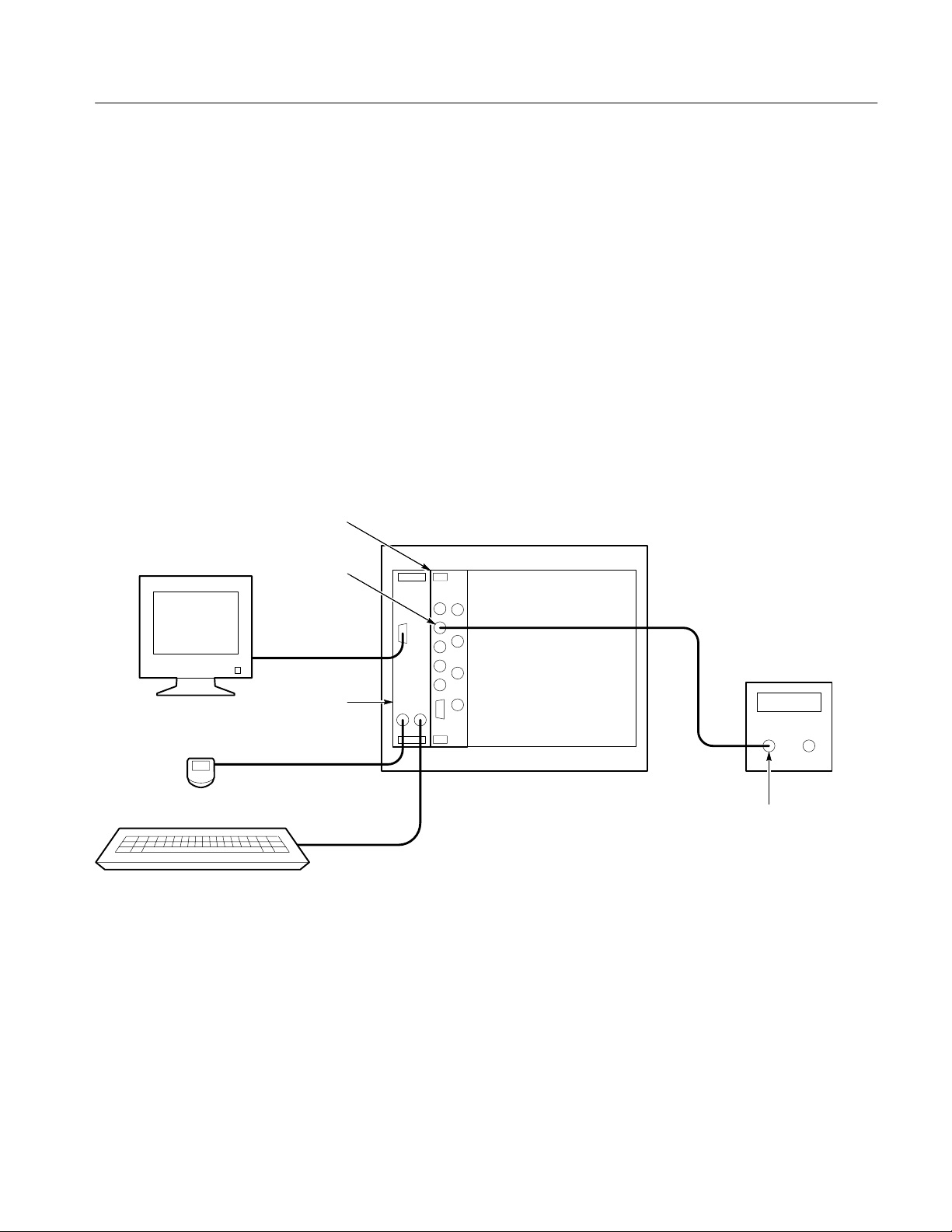
Functional Tests
Incoming Inspection Procedure
The following procedures test the internal time and voltage references of the
waveform analyzer. You will need a frequency counter, digital multimeter,
coaxial cable with BNC connectors, and a dual-banana to BNC adapter to
perform the Functional Tests. See the equipment requirements on page 1–13.
Measure Time Reference
Monitor
Mouse
(optional)
This procedure tests the accuracy of the internal time reference
(10 MHz 1 kHz).
1. Connect a coaxial cable from the frequency counter input to the REF-
ERENCE OUTPUT connector (see Figure 1–4).
2. Send the following command to initialize the waveform analyzer:
TVS600
Reference
Output
Slot 0
Controller
VXI mainframe
Frequency
Counter
Keyboard
Figure 1–4: Time Reference Test Setup for Functional Tests
TVS600 Series Waveform Analyzers User Manual
Input
1–17
Page 40

Incoming Inspection Procedure
3. Select the following settings for the frequency counter:
Mode Frequency
Trigger Internal
Attenuation X1
4. Send the following command to turn on the time reference:
OUTP:REF:FUNC CLOC;:OUTP:REF ON
5. Check the frequency counter display. The frequency must be between
9,999,000 Hz and 10,001,000 Hz.
6. Disconnect the frequency counter from the REFERENCE OUTPUT
connector.
7. Proceed to Measure Voltage Reference to continue the Incoming Inspection
Procedure.
1–18
TVS600 Series Waveform Analyzers User Manual
Page 41

Incoming Inspection Procedure
Measure Voltage
Reference
Monitor
Mouse
(optional)
Keyboard
This procedure tests the accuracy of the internal voltage reference (+8 V 1%).
1. Use a coaxial cable and dual-banana to BNC adapter to connect the digital
multimeter input to the REFERENCE OUTPUT connector (see Figure 1–5).
TVS600
Reference
Output
Slot 0
Controller
VXI mainframe
Digital Multimeter
–
+
Dual banana to
BNC adapter
Figure 1–5: Voltage Reference Test Setup for Functional Tests
2. Send the following command to initialize the waveform analyzer:
*RST
3. Select the following digital multimeter control settings:
Mode DC Volts
Scale 20
4. Send the following command to turn on the voltage reference:
OUTP:REF:FUNC VOLT;:OUTP:REF ON
5. Check the digital multimeter display. The voltage must be between +7.92 V
and +8.08 V.
6. Disconnect the digital multimeter from the REFERENCE OUTPUT
connector.
7. Proceed to Self Cal to continue the Incoming Inspection Procedure.
TVS600 Series Waveform Analyzers User Manual
1–19
Page 42

Incoming Inspection Procedure
Self Cal
The Self Cal uses internal routines and the internal time and voltage reference to
generate data such as gain and offset values, to optimize the waveform analyzer
performance at the current ambient temperature. The data is stored in memory
for use until you perform another self cal. No test equipment is required.
1. Send the following command to execute the internal self cal routines:
CAL
2. Wait for the self cal to complete.
H When running self cal, the READY, ACCESSED, ARM’D, and TRIG’D
indicators blink
H The self cal takes 15 to 30 minutes to complete
3. Send the following query to check the self cal results:
CAL:RES?
4. Read the self cal results.
H A 0 result indicates all tests passed successfully
H A –1 result indicates the self cal is still in progress; wait five minutes
and send the CAL:RES? query again to read the test results
H A 2000 to 2999 result indicates self cal failures and a need for service on
the failed module.
This completes the Incoming Inspection Procedure. If all tests passed, the
waveform analyzer is ready for use. If any test failed, refer the module for
service.
1–20
TVS600 Series Waveform Analyzers User Manual
Page 43

Operating Basics
This section contains information that can help you operate the TVS600
Waveform Analyzer more effectively. The section includes the following
topics:
H Connectors and Indicators, on page 2–3, describes how to use the front
panel connectors and what information the indicators convey.
H Functional Overview, on page 2–7, describes how the the main functions of
the waveform analyzer operate and how to use the related commands to
control these functions.
H Instrument I/O, on page 2–63, describes how the VXIbus and RS-232
interfaces are configured.
H Tutorial, on page 2–71, presents a step-by-step tutorial that shows you how
to use the command set to configure the waveform analyzer to acquire
waveforms and perform many of its main functions.
For information on configuring and installing your waveform analyzer, refer to
Getting Started.
TVS600 Series Waveform Analyzers User Manual
2–1
Page 44
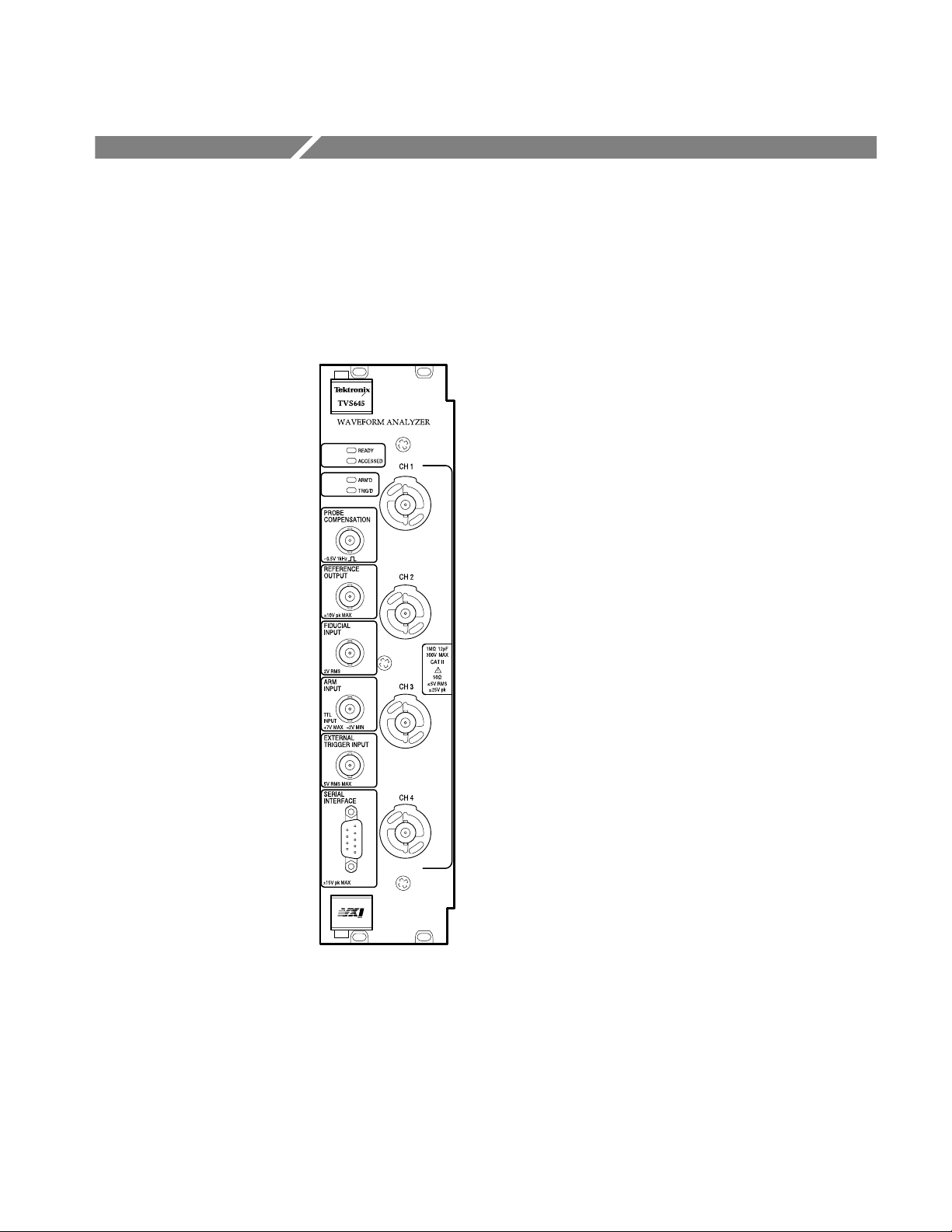
Connectors and Indicators
Figure 2–1 shows the connectors and indicators on the front panel of a four-channel waveform analyzer. The two-channel model looks and operates the same, but
without the CH 3 and CH 4 inputs. Descriptions of each connector and indicator
follow the illustration.
Figure 2–1: TVS600 Front Panel
CH1, CH2, CH3, and CH4 Channel Inputs. These BNC input connectors drive the
vertical channel amplifiers and their dedicated digitizers. If your instrument is a
TVS641 or TVS645, it has four input channels as shown in Figure 2–1.
Otherwise, the TVS621 and TVS625 provide only the top two channels. Each
TVS600 Series Waveform Analyzers User Manual
2–3
Page 45

Connectors and Indicators
channel supports TekProbe Level 1 and Level 2 probes which offer many
features, including signal offset.
The signal inputs can be set for 1 M or 50 input impedance. Coupling
selections are DC, AC, and Ground. The Ground setting connects the internal
amplifier to ground, but presents an open circuit impedance (w500 k) to your
signal.
Every input channel has automatic input protection when set to 50 coupling.
When coupling is set to 50 and an input signal exceeds the input range of an
input channel, the coupling for that channel is set to 1 M to protect the
attenuator and digitizer.
For more information, refer to the description of the INPut commands starting on
page 3–123.
READY Indicator. The green LED lights continuously after the waveform analyzer
powers up and completes power-on diagnostics successfully. During normal
operation, READY blinks when an error occurs that generates a status message.
ACCESSED Indicator. The yellow LED blinks on and then off under the following
conditions:
H Each time communication with the waveform analyzer occurs
H When the Slot 0 resource manager asserts the Module Identification
(MODID) line
ARM’D Indicator. The green LED lights when the waveform analyzer is armed and
ready to accept a trigger signal.
TRIG’D Indicator. The green LED lights briefly when a trigger occurs for the
current acquisition. The TRIG’D Indicator lights continuously whenever trigger
events occur more often than three per second.
PROBE COMPENSATION. The BNC output provides a 1 kHz square wave signal
for adjusting probe compensation. The signal amplitude is 0.5 V peak-to-peak
into a 1 M load. To enable the compensation signal, send the command
OUTP:PCOM ON.
REFERENCE OUTPUT. The BNC output provides access to two internal references; the DC calibrator reference voltage or the time base clock. The precision
calibrator reference voltage (VOLT) is +8.0 V. The time base clock (CLOC) is a
10 MHz square wave. Amplitude is w1 V into a 50 load. To select a reference
signal, send the command OUTP:REF:FUNC [CLOC|VOLT]. To enable the
2–4
TVS600 Series Waveform Analyzers User Manual
Page 46

Connectors and Indicators
selected signal to the REFERENCE OUTPUT connector, send the command
OUTP:REF ON.
FIDUCIAL INPUT. The BNC input provides a way to add a signal component to
the Channel 1 input signal. Adding a common timing signal to Channel 1 on
several instruments provides a way to improve cross timing between multiple
instruments. The input range is 1 V. The input resistance presents 0.01 mF in
series with 50 W.
ARM INPUT. The BNC input allows you to arm the acquisition system by
grounding the center lead. The ARM input is level sensitive and is not latched.
An internal pull up resistor connected to +5 V maintains a high level until you
ground the input. You must maintain a ground state on the center lead until the
Trigger event occurs.
EXTERNAL TRIGGER INPUT. The BNC input provides a connection for an
external trigger source. The input has 50 W impedance and is DC coupled only.
Trigger signals as large as 5 V (DC + Peak AC) may be applied.
SERIAL INTERFACE. The subminiature D connector provides a serial interface for
controlling the waveform analyzer and reading acquired data. Refer to page 2–29
for the RS-232 pin assignments. You can configure the serial interface with the
commands in the SYST:COMM:SER subsystem.
TVS600 Series Waveform Analyzers User Manual
2–5
Page 47

Functional Overview
This section describes how the main subsystems of the waveform analyzer
operate and the commands you use to control them. The initial discussion
describes how the subsystems operate together. Following the overview each of
the following topics is described in detail:
H Acquisition, page 2–9
H Vertical Range and Offset, page 2–19
H Triggering, page 2–21
H Calculations and Measurements, page 2–31
H Fast Data Channel, page 2–50
H Data Transfers, page 2–55
System Operation
The waveform analyzer is a multi-channel, high-speed digitizing VXIbus
module. In addition to acquiring high-resolution waveforms, the waveform
analyzer performs waveform transformations and automated measurements. The
transfer of acquired data to the VXIbus controller can use the traditional word
serial protocol or the Fast Data Channel, which provides a very high transfer
rate.
Control of all these instrument functions is accomplished with the software
command set. The waveform analyzer commands follow the SCPI 1995.0
standard for a sensing instrument. Figure 2–2 shows the organization of the
waveform analyzer following the SCPI model.
In Figure 2–2, signals enter at the left through the INPut channels and measurement data exits at the right with the TRACe commands. The identifying number
for each channel is used to identify corresponding operations in other blocks. For
example, to set the input impedance for CH 1 you use the INPut1 command and
to set the vertical range of CH1 you use the VOLTage1 command. Likewise, you
configure the CH 2 input with the INPut2 and VOLTage2 commands. The four
CALCulate function blocks, which perform calculations on any selected input,
are an exception to this model.
The TRIGger block in Figure 2–2 controls when to acquire data by setting the
trigger event. You can control when trigger events are allowed with the ARM
function and its independent front-panel connection. Once the TRIGger block is
armed, you can trigger on a TRIGgerA event followed by any defined TRIGgerB
TVS600 Series Waveform Analyzers User Manual
2–7
Page 48

Functional Overview
event. Alternately, you can trigger on different pulse parameters based on
settings in the TRIGger:PULSe subsystem.
The discussions following Figure 2–2 describe how to control the major
instrument functions and which commands to use.
CH1..4
INPut1..4 VOLTage1..4
SWEep
ROSCillator
ABORt
INITiate
[SENSe:]
AVERage
AADVance
TRIGger
Idle
ARM
FUNCtion
DATA
TRACe
CHAN1..4
AATS
CALC1..4
WSP
or
FDC
TRIGger[:A]
TRIGger:B
Figure 2–2: Instrument model showing root level nodes
2–8
CALCulate1..4
TVS600 Series Waveform Analyzers User Manual
Page 49
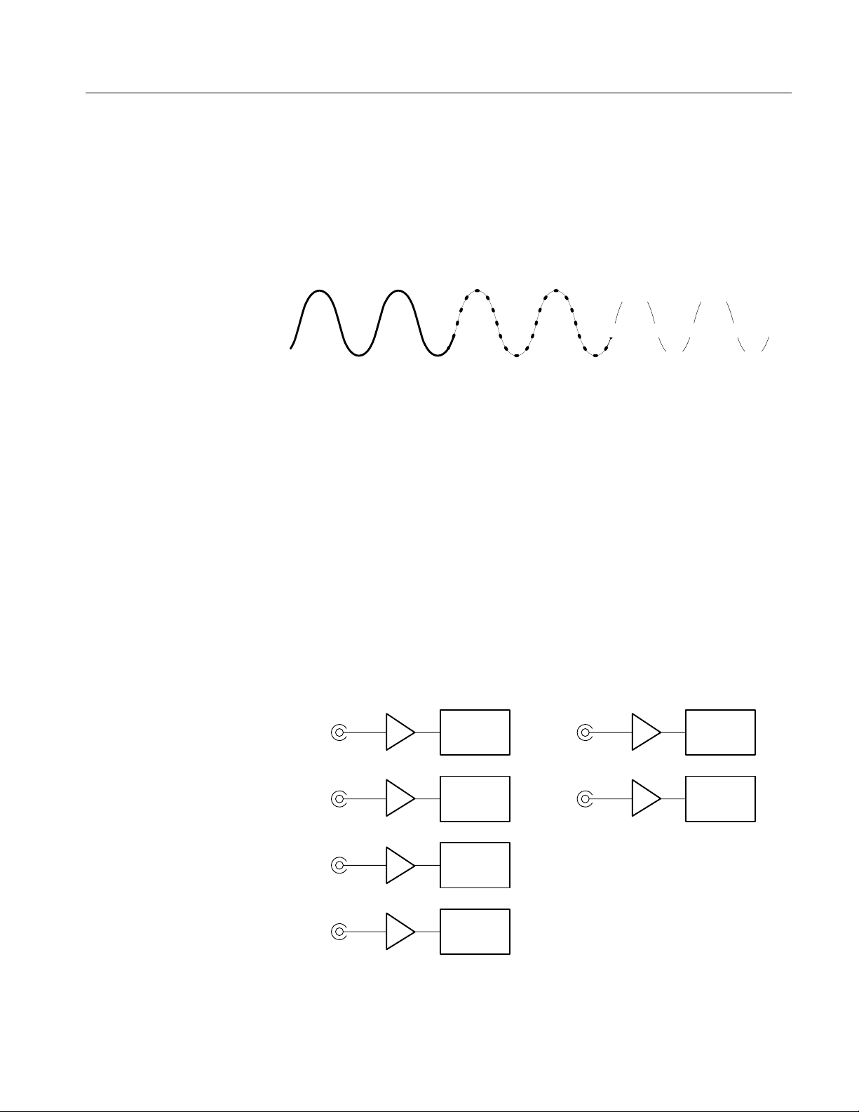
Acquisition
Functional Overview
Acquisition is the process of sampling an analog input signal, converting it into
digital data, and assembling it into a waveform record. The waveform analyzer
samples the voltage level of the input signal at regular time intervals. The signal
parts within the vertical range of the amplifier are digitized. See Figure 2–3.
Acquisition Hardware
+5.0 V
0 V 0 V 0 V 0 V
Input signal Sampled points Digital values
–5.0 V
+5.0 V
–5.0 V
Figure 2–3: Digital acquisition showing sampling and digitizing steps
The sampled points are stored in memory as a waveform record. The waveform
record includes the signal source, trigger point location, and horizontal and
vertical scaling. Once the signal is acquired, you can use the CALCulate
subsystem to perform measurements or to transform the digital waveform record.
The waveform analyzer has other types of acquisition, such as Averaging and
Enveloping, that produce enhanced waveform records. Refer to Modes of
Acquisition on page 2–12 and Averaging and Enveloping on page 2–18.
Each channel has a dedicated input amplifier and digitizer as shown in
Figure 2–4.
Two channel modelsFour channel models
CH 1
CH 2
CH 3
CH 4
Figure 2–4: Digitizer configuration
TVS600 Series Waveform Analyzers User Manual
Digitizer
Digitizer
Digitizer
Digitizer
CH 1
CH 2
Digitizer
Digitizer
2–9
Page 50

Functional Overview
Acquisition Parameters
The waveform analyzer uses a set of common parameters to acquire waveforms
from all active channels. These common parameters include the sample interval,
record length, trigger point, and the number of samples acquired before
(pretrigger) and after (posttrigger) the trigger point. Figure 2–5 shows the trigger
point and the pretrigger samples taken before the trigger point.
Sample Interval. The sample interval is the precise time between sample points
taken during acquisition. Figure 2–5 shows the sample interval between two
waveform samples. The shorter the sample interval, the more detail you acquire
for a particular waveform feature. However, short sample intervals reduce the
duration of the total waveform record. If you wish to capture many cycles of a
waveform, you will likely need to use a longer sample interval. Use the
command SWEep:TINTerval to set the sample interval. The sample interval is
the reciprocal (1/x) of the sample rate.
Sample interval
Trigger event
Pretrigger
samples
Posttrigger
samples
Figure 2–5: Digital sampling showing the sample interval, trigger event, and
pretrigger samples
Record Length. The number of samples required to fill a waveform record is the
record length. Use the command SWeep:POINts to set or query the number of
samples in the waveform record. All channels share the record length setting.
You can set the record length from 256 to 15,000 for real-time acquisition. A
record length of 30,000 is available in the extended realtime mode. The time
window or duration of the waveform record is equal to the
Record Length * Sample Interval.
You can also set the record length as a time period with SWEep:TIME. The
relationship between SWEep:POINts and SWEep:TIME is as follows:
SWEep:TIME = SWEep:TINTerval*SWEep:POINts
2–10
TVS600 Series Waveform Analyzers User Manual
Page 51

Functional Overview
SWEep:TINTerval sets the sample interval. For more information, refer to
Sample Interval on page 2–10 and Acquisition Modes on page 2–12.
Trigger Point. The trigger point marks the time zero in a waveform record. All
waveform samples are located in time with respect to the trigger point. You can
define the trigger point as a simple level and slope crossing, as a number of such
trigger events, or upon detection of a defined type of pulse. Figure 2–5 shows a
simple level and slope based trigger point. For information on the trigger system,
refer to the discussion Triggering on page 2–21.
Waveform Record Position. You can position the waveform record relative to the
trigger point to acquire pretrigger and posttrigger samples. The trigger point can
occur anywhere within the waveform record. Note that all concurrent acquisitions share the record position settings.
The commands that position the waveform record are SWEep:OFFSet and
SWEep:OREFerence. Figure 2–6 shows how these commands position the
waveform record relative to the trigger point. You can set SWEep:OFFSet as a
number of record points (:POINts) or as a period of time (:TIME).
For example, to acquire 50% pretrigger sample points in a 1024 point waveform
record, set :OREFence:LOCation to zero and set :OFFSet:POINts to –512. Now
the trigger is horizontally centered in the record; half the samples are in the
pretrigger region and half in the posttrigger region.
The trigger circuit, with its event count, time delay, and holdoff capabilities is
controlled independently from the record positioning functions of the SWEEp
commands.
For more information, refer to the SWEep commands starting on page 3–169.
For trigger information, refer to Triggering on page 2–21.
TVS600 Series Waveform Analyzers User Manual
2–11
Page 52

Functional Overview
Positioning the waveform record using
SWEep:OREFerence
SWEep:OREFerence = 0
SWEep:OFFSet = 0
Waveform record
SWEep:OREFerence = .5
SWEep:OFFSet = 0
Waveform record
Positioning the waveform record using
SWEep:OFFSet
SWEep:OREFerence = 0
SWEep:OFFSet = 0
Waveform record
SWEep:OREFerence = 0
SWEep:OFFSet = –1/2 record length
Waveform record
Modes of Acquisition
SWEep:OREFerence = 1
SWEep:OFFSet = 0
Waveform record
SWEep:OREFerence = 0
SWEep:OFFSet = – record length
Waveform record
Indicates trigger point
Figure 2–6: Positioning the waveform record relative to the trigger point
The waveform analyzer provides two modes of acquisition: real time and
extended real time. Real-time acquisition is the normal mode after the reset
command, *RST. The waveform analyzer switches from real-time to extended
real-time acquisition when the sample interval setting is 100 ns or longer.
Extended real time acquisition provides up to 30,000 point record lengths. The
real-time and extended real-time acquisition modes may be used with the
2–12
TVS600 Series Waveform Analyzers User Manual
Page 53

Functional Overview
auto-advance acquisition cycle, which provides very fast rearm time. Figure 2–8
on page 2–14 shows the auto-advance acquisition cycle.
Real Time Acquisition. With real-time acquisition, the waveform record is filled
serially by the digitizers based on a single trigger event. Figure 2–7 shows how
real-time acquisition acquires samples in a linear fashion. Because real-time
acquisition requires only one trigger event, it is effective for capturing rare or
non-repeating events.
Record Points
Sampling Rate
Figure 2–7: Real-time acquisition
Extended Real-Time Acquisition. With extended real-time acquisition, you can
acquire a waveform record up to 30,000 points. The waveform record fills
serially with only one trigger event. Extended real-time acquisition is available
whenever the sample interval is 100 ns or longer, no explicit command is
necessary. However, you do need to explicitly set the record length to 30000
after switching to extended real time acquisition if you want the longest record.
Auto-Advance Acquisition. Auto-advance acquisition provides the fastest
acquisition rearm time by skipping certain system processing until all waveforms
are acquired. Figure 2–8 shows the Auto-advance acquisition loop. For more
information see Auto-Advance Acquisition on page 2–15.
TVS600 Series Waveform Analyzers User Manual
2–13
Page 54

Functional Overview
Acquisition Cycle
The acquisition cycle follows common steps, but you can select from two types
of acquisition looping. The acquisition cycle proceeds through the steps shown
in Figure 2–8.
INITiate:COUNt
Auto-advance acquisition
Start
acquisition
(INITiate)
Trigger
enabled
Pretrigger
time
Posttrigger
waveform
acquisition
Data out of
acquisition
memory
System
processing
Measurements/
calculations
Data to
VXI shared
memory
Idle
Figure 2–8: The acquisition cycle
A brief description of each acquisition block follows:
H The INIT command is always required to start acquisition. INIT puts the
acquisition system in the active state awaiting an arm or trigger signal.
H During the pretrigger time, the acquisition system initializes itself and the
digitizer acquires any pretrigger record points specified with the SWEep
commands.
H Before the trigger enabled event occurs, any specified ARM event must
occur and all required pretrigger samples must be acquired. Once enabled,
the next valid TRIGger:A event is accepted.
H During the posttrigger waveform acquisition period, the active channel
digitizers acquire all posttrigger waveform samples needed to fill the defined
waveform records.
H In the data out of acquisition memory block, the digitizers transfer acquired
data out of acquisition memory and into DSP memory.
As shown in Figure 2–8, acquisition normally proceeds at this point with system
processing and any specified measurements or calculations. After processing
completes, the resultant waveform records are moved to VXIbus shared memory
for transfer to your system controller.
Acquisition Looping. The waveform analyzer provides two different ways to loop
or cycle through a specified number of acquisitions. You might choose acquisition looping in order to capture a series of waveform records or measurements
over a period of time. The two methods are auto-advance acquisition mode
(AADV commands) and INIT looping.
2–14
TVS600 Series Waveform Analyzers User Manual
Page 55
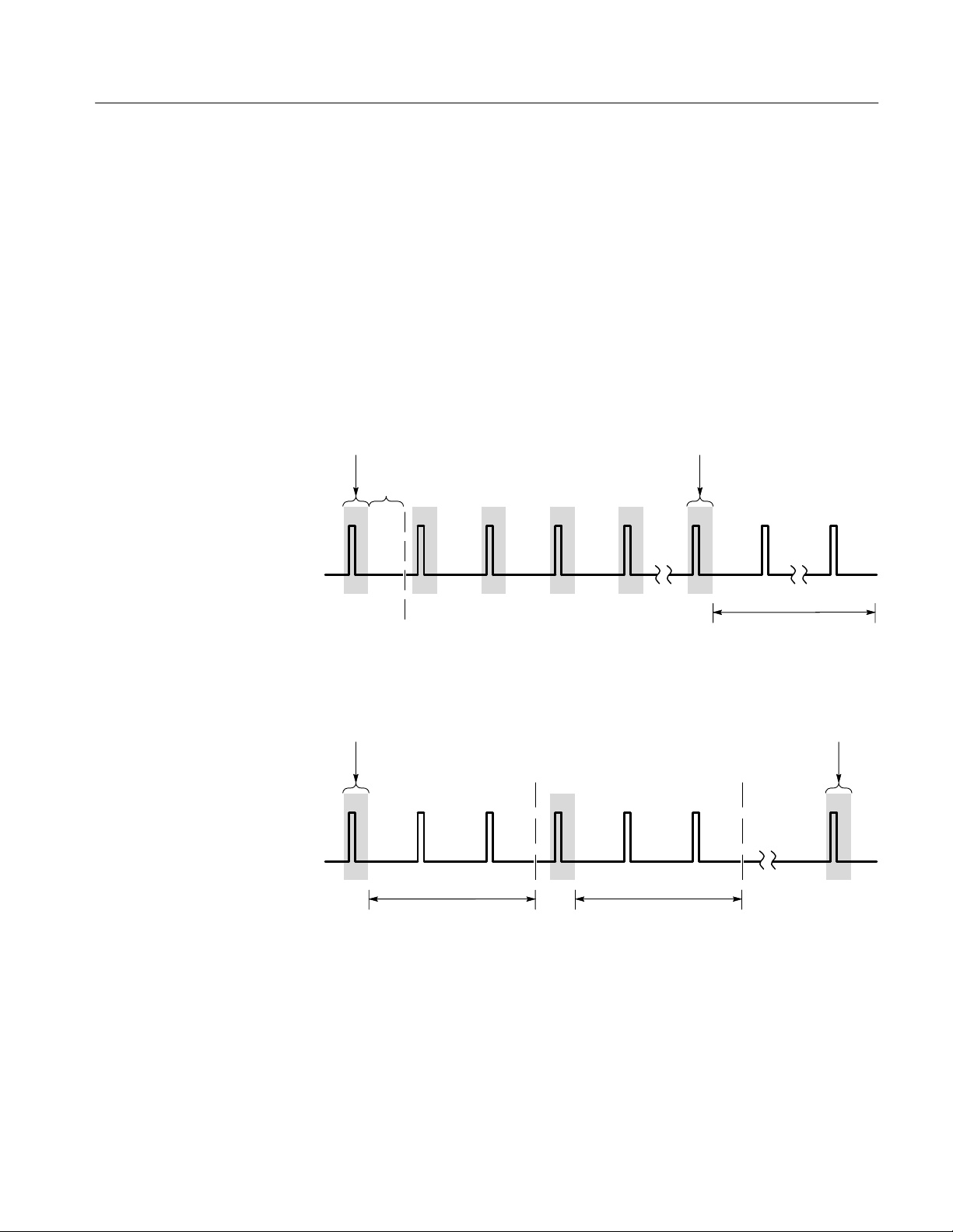
Functional Overview
Auto-advance provides the fastest cycle time but does not perform and return
measurement results until all acquisitions complete. Figure 2–9 compares the
acquisition cycle time between auto-advance acquisition and INIT looping.
When auto-advance acquisition is active, system processing starts on the
auto-advance waveforms when the last acquisition loop completes. With the
INIT:COUNt looping mode shown in Figure 2–8, all processing completes and
measurement results return before another acquisition cycle begins. In singleshot acquisition (no looping enabled), the acquisition system returns to the Idle
state after acquisition completes.
Acquisition looping with
AADVance:COUNt <n>
First record
Rearm
time
Trigger
enabled
Acquisition looping with
INITiate:COUNt <n>
First record
Trigger
enabled
nth record
system processing and
T
Sn
transfer of all AADV waveforms
Trigger
enabled
nth record
system processing and
T
S1
transfer of first waveform
Figure 2–9: Comparison between auto-advance and INIT acquisition looping
Auto-Advance Acquisition
Auto-advance acquisition acquires a sequence of waveform records with minimal
delay between acquisitions. As shown in Figure 2–8, auto-advance acquisition
provides the fastest acquisition cycle time because the system processing,
measurement, and data transfer tasks are delayed until acquisition completes.
TVS600 Series Waveform Analyzers User Manual
T
system processing and
S2
transfer of second waveform
2–15
Page 56

Functional Overview
Another feature of auto-advance acquisition is that each waveform record
includes a timestamp which records the time between consecutive waveform
records. Timestamp resolution is 125 ns.
Many of the basic settings for auto-advance acquisition are the same as for
normal acquisition. You enable channels, define the record length and sample
interval.
Several additional steps are necessary to configure auto-advance acquisition.
First, enable the auto-advance mode with the command AADVance:STATe ON.
Next, specify the number of waveform records to acquire with the command
AADVance:COUNt <n>. You can set :COUNt to fill acquisition memory with
waveform records by giving :COUNt the value MAX or 0 (zero).
The Timestamp. During auto-advance acquisition, the time between consecutive
waveform records is recorded in a timestamp record. The timestamp record has
the trace name AATS and is available with the transfer commands TRACe?,
TRACe:COPY, etc. The record contains a sequence of times in seconds, from t0
to tn, separated by commas. Set the format of the AATS record to ASCII or
32-bit REAL numbers with the command FORM:TRAC:AATS.
Fast Data Channel and
Auto-Advance Acquisition
The Fast Data Channel (FDC) provides a fast transfer protocol for moving
waveform records and other data between the waveform analyzer and a VXIbus
controller. The waveform analyzer includes an FDC driver that provides the
instrument side of the protocol. To use FDC, you must do the following tasks:
H Ensure that controller used provides support for the FDC protocol. (The
VXIplug&play VISA I/O interface provides FDC support.)
H Open two sessions with the waveform analyzer, one for sending ASCII
commands and another for FDC data transfer.
H Configure the FDC session to use the FDC protocol (by setting VISA
attributes — see step 10 in the example).
H Use the ASCII session to set up the waveform analyzer, acquire the data, and
initiate its transfer.
When configuring the ASCII and FDC sessions, you must perform setup steps in
proper order:
H The number of active channels and the record length must be set before you
enter the number of waveform records to acquire with AADVance:COUNt.
The waveform analyzer automatically computes the maximum (MAX)
2–16
TVS600 Series Waveform Analyzers User Manual
Page 57

Functional Overview
AADV:COUNt value based on the number of active channels and the record
length.
H You must make all acquisition settings and configure the FDC configuration
before issuing the INITiate command to begin acquisition.
The following example shows the steps necessary to set up an auto-advance
acquisition with FDC data transfer, observing the principles listed above. The
example assumes you want to acquire CH1 and CH2.
1. Enable the channels to acquire with the command FUNC:ON “XTIM:VOLT
1”,“XTIM:VOLT 2”.
2. Set the individual channel parameters, such as voltage range.
3. Set the trigger parameters.
4. Set the waveform record length with SWE:POIN and the sample interval
with SWE:TINT.
5. Enable auto-advance acquisition with the command AADV:STAT ON.
6. Specify the number of waveform records to acquire with the command
AADV:COUN command. The value MAX acquires enough waveform
records to fill DSP memory.
7. Specify the number of waveform records to transfer over the FDC with the
command AADV:REC:COUN. The value MAX selects all acquisitions,
from :STARt on, for transfer.
8. Specify the list of signal sources to transfer with the command TRAC:LIST.
You may have an active channel but not select it for transfer. In this example,
use TRAC:LIST CHAN1,CHAN2. The value AATS selects the timestamp
record for the auto-advance waveform records that you will acquire.
9. You can choose to skip the transfer of the first acquisition records for both
channels if, for example, you think the device under test might initially be
unstable. To skip just the first two waveform records, specify the number of
the waveform record to begin FDC transfers using the command
AADV:REC:STAR 3 which skips over records 1 and 2.
TVS600 Series Waveform Analyzers User Manual
2–17
Page 58

Functional Overview
10. Configure the FDC session to use the FDC protocol by setting the following
VISA attributes using the function:
viSetAttribute (vi_session, attr_name, attr_value)
Attribute Name
Attribute Value
VI_ATTR_FDC_CHNL
1
VI_ATTR_FDC_MODE
VI_FDC_STREAM
VI_ATTR_IO_PROT
VI_FDC
11. Start acquisition on the waveform analyzer with the INITiate command.
Acquisition begins.
12. Use the VISA function viRead (fdc_session, buf, buf_size, return_count) to
transfer the acquisition from the waveform analyzer to the character array
buffer of the controller.
Average and Envelope
Waveforms
For more information, refer to Auto-Advance Acquisition on page 2–15,
Acquisition Cycle on page 2–14, and Fast Data Channel on page 2–50.
Additionally, refer to the command descriptions in Chapter 3, Syntax and
Commands.
Averaging and enveloping acquisition modes combine a number of acquisitions
in one waveform record. Averaging accumulates an average value for each record
point over many acquisitions to provide higher vertical resolution. Enveloping
finds the highest and lowest sample values over many acquisitions to produce a
waveform record of alternating maximum and minimum values. The commands
in the AVERage subsystem control averaging. All active channels are affected by
the AVERage setting. Averaging and enveloping occur in the acquisition system
before waveform records are passed to the CALC blocks. An averaged waveform
can often produce a more accurate measurement.
To enable averaging, set AVERage ON and specify the number of waveform
records to average with AVERage:COUNt. Use the command AVERage:TYPE
to select averaging (SCALar) or enveloping (ENVelope).
For more information, refer to the command descriptions in Chapter 3, Syntax
and Commands.
2–18
TVS600 Series Waveform Analyzers User Manual
Page 59

Vertical Range and Offset
The vertical range and offset for the waveform analyzer input channels are
individually controlled. The controlling commands are in the VOLTage
subsystem, described on page 3–247. To set the vertical scaling for an input
channel you actually set the vertical range and the offset of the channel digitizer.
The offset value sets the voltage level that is at the middle of the digitizer range.
The waveform analyzer provides two methods of setting the vertical range and
offset: RANGe and OFFSet, and UPPer and LOWer. Figure 2–10 shows how
these two methods are used and presents several offset examples. Note in the
example that it is the input vertical range or “window” of the digitizer that is
moved by vertical OFFset and not the DC level of the input signal. Applying a
negative OFFset moves the vertical range down. Likewise, applying a positive
OFFset moves the vertical range up. You can use the UPPer and LOWer
parameters to set the range to absolute vertical values if you prefer.
Valid waveform data are in the range +32256, for waveform values that equal
VERTical:RANGe UPPer, to –32256, for waveform values that equal VERTical:RANGe LOWer.
Functional Overview
Parts of a waveform that exceed the range are clipped. Parts that exceed the most
positive range limit (UPPer) are acquired as Overrange points and are assigned
the value +32767. Parts that exceed the most negative range limit (LOWer) are
acquired as Underrange points and are assigned the value –32767.
TVS600 Series Waveform Analyzers User Manual
2–19
Page 60
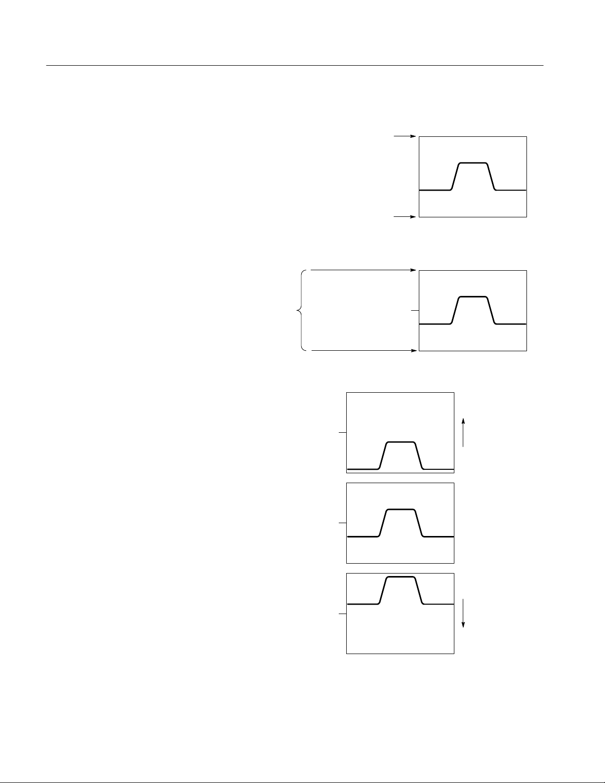
Functional Overview
Setting vertical range with upper and lower limits
VOLTage:RANGe:UPPer
VOLTage:RANGe:LOWer
Setting vertical range with offset and peak-to-peak range
VOLTage:RANGe:PTPeak
(range is centered on
offset value)
VOLTage:RANGe:OFFSet
Examples:
VOLTage:RANGe:OFFSet +2.0 V
VOLTage:RANGe:OFFSet –2.0 V
VOLTage:RANGe:PTPeak 5 V
Acquisition
window shifts
positive
VOLTage:RANGe:OFFSet 0.0 V
Acquisition
window shifts
negative
2–20
Figure 2–10: Setting vertical range and offset of input channels
TVS600 Series Waveform Analyzers User Manual
Page 61
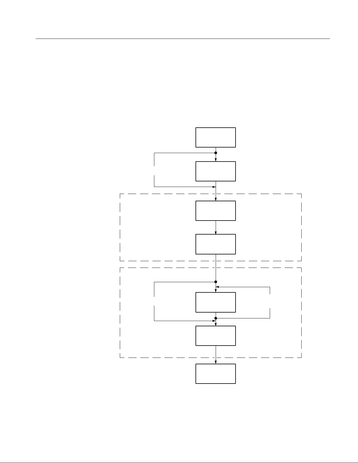
Triggering
Functional Overview
Triggering determines when the waveform analyzer acquires a waveform record.
The trigger system parameters, such as trigger level and slope, determine at what
point on a waveform the trigger event occurs. Figure 2–11 shows the waveform
analyzer Arm/Trigger cycle that all acquisitions follow. The illustrated cycle
follows the SCPI standard for triggering.
INITiate TRIGger:A
and TRIGger:B
ARM:SOURce IMMediate
TRIGger:A (SEQuence 1)
TRIGger:B (SEQuence 2)
TRIGger:B:SOURce IMMediate
ARM Event
TRIGger:A Event
TRIGger:A:DELay
(delayed by time)
TRIGger:B Event
TRIGger:B:DELay
(delayed by time)
TRIGger:B:ECOunt
(delay by events)
Figure 2–11: The Arm/Trigger cycle
TVS600 Series Waveform Analyzers User Manual
Acquire signal(s)
2–21
Page 62

Functional Overview
The TRIGger:A and TRIGger:B delay capabilities shown in Figure 2–11 provide
many delayed trigger modes.
The Trigger Event
Trigger Sources
The trigger event establishes the time-zero point (t
) in the waveform record. The
0
time locations of all points in the waveform record are relative to the trigger
point. Once the waveform analyzer detects a trigger event, it ignores triggers
until the acquisition completes and trigger holdoff expires. You can define a
trigger event as a simple edge trigger, a delayed trigger, or a pulse trigger.
Regardless of the type of triggering, you need to choose a trigger source.
The trigger source is the signal monitored for a trigger event. Table 2–1 lists the
possible trigger sources and their compatibility with each trigger type.
T able 2–1: Trigger Sources and Compatibility
Trigger Type
Trigger Source Description
Input channels
CH1, CH2, CH3
CH4 (depending
on model)
External Trigger Selects the input connector EXTERNAL
VXIbus Triggers These digital trigger signals from the VXI bus
IMMediate Effectively bypasses the TRIGger:B event
Provide triggering from signals connected to
the input channels. Parameters include
coupling (AC/DC), level, slope, and trigger
filters. Trigger filters (:LPASs, HPASs, and
NREJ) are available to eliminate low or high
frequency elements. The channel you select
as a trigger source need not be acquired.
TRIGGER INPUT on the waveform analyzer
front panel. The input is DC coupled and has
a maximum range of 1 V . The available
trigger settings are slope and level.
are available to all VXI modules. The
waveform analyzer can trigger off and drive
eight TTL logic trigger lines (TTLTrg0 –
TTL Trg7) and two ECL logic trigger lines
(ECL Trg0 and ECLTrg1). The TTLTrg lines
have a 12.5 Mhz clock speed and the ECLTrg
lines 62.5 Mhz. The waveform analyzer can
source the TTLTrg lines with any valid trigger
source. Refer to the OUTPut:TTLTrg
commands starting on page 3–144.
detector.
EDGE
TRIG:A
n n n
n n
n
EDGE
TRIG:B
n
TRIG
:PULSe
2–22
TVS600 Series Waveform Analyzers User Manual
Page 63

Functional Overview
Trigger Coupling
Trigger coupling determines which frequency components of an analog trigger
signal are passed to the trigger system. The VXIbus trigger sources are digital
signals and do not provide coupling selections. The External trigger provides DC
coupling only. TRIGger:A and TRIGger:B provide a variety of trigger coupling
selections with the TRIGger:A and TRIGger:B COUPling commands, when
using the input signals.
Aside from the basic AC and DC coupling, the waveform analyzer offers several
coupling preset commands that also control trigger filtering and noise rejection.
The coupling selections are as follows:
H DC passes all of the input signal. In other words, it passes both AC and DC
components to the trigger circuit.
H AC passes only the alternating components of an input signal. It removes the
DC component from the trigger signal.
H HFReject removes the high frequency portion of the triggering signal. Only
the low frequency components pass on to the triggering system to start an
acquisition. High frequency rejection attenuates signals above 50 kHz.
H LFReject removes the low frequency portion of the triggering signal. Only
the high frequency components pass on to the triggering system to start an
acquisition. Low frequency rejection attenuates signals below 50 kHz.
Slope and Level
H ACNReject provides noise rejection while rejecting the DC portion of
the signal.
H DCNReject provides noise rejection but passes all other portions of
the signal.
The slope and level settings determine the analog parameters for the trigger point
for edge triggering. Figure 2–12 shows the commands that control each
parameter. The trigger level must be within the signal range to cause a trigger
event. The slope setting allows you to capture the rising or falling edge of
a signal.
TRIGger:SLOPe
(positive or negative)
TRIGger:LEVel
Figure 2–12: Slope and level define the trigger event
TVS600 Series Waveform Analyzers User Manual
2–23
Page 64
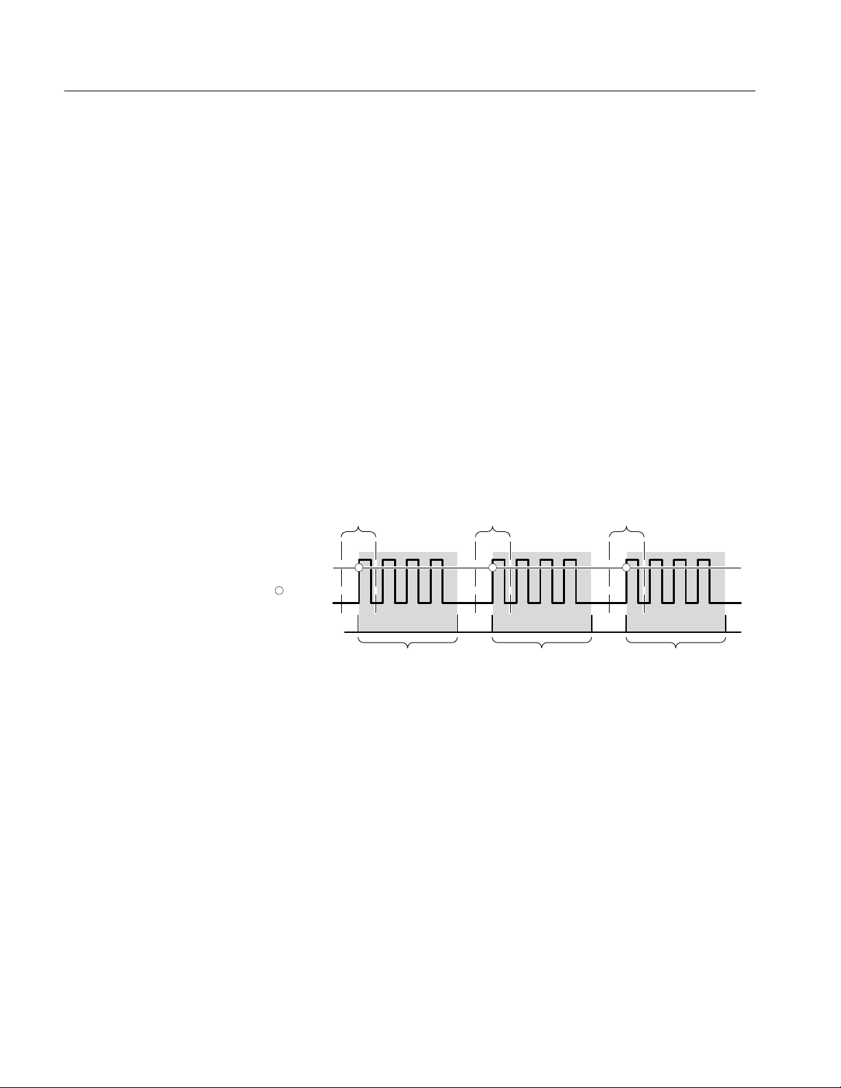
Functional Overview
Trigger Position
Trigger Holdoff
The trigger position defines where on the waveform record the trigger occurs. It
lets you properly align and measure data within records. The part of the record
that occurs before the trigger is the pretrigger portion. The part that occurs after
the trigger is the posttrigger portion.
For information on setting the trigger position refer to Waveform Record Position
on page 2–11.
When the waveform analyzer recognizes a trigger event, it disables the trigger
system until acquisition and trigger holdoff complete. Trigger holdoff starts
when the trigger event occurs as shown in Figure 2–13. As shown in the
illustration, you can set the holdoff time to skip signal pulses that would cause
false triggering. Without trigger holdoff, pulses two, three, and four would be
valid trigger events assuming sufficient time for acquisition and rearming. The
desired trigger event is the first rising edge of each group of pulses. Note that the
waveform record has 50% of its samples before the trigger point.
The holdoff range is from 250 ns (minimum) to 12 seconds (maximum).
Waveform
record
Waveform
record
Waveform
record
Trigger level
Indicates
trigger points
Holdoff
(TRIGger:HOLDoff:TIME)
Triggers are not recognized during holdoff time.
Waveform records are shown with 50% pretrigger
samples.
Holdoff
Figure 2–13: Trigger holdoff time ensures valid triggering
Holdoff
2–24
TVS600 Series Waveform Analyzers User Manual
Page 65

Functional Overview
Trigger Types
Automatic Trigger Mode
The waveform analyzer provides two standard trigger types: edge and pulse. Use
the command TRIGger:TYPE to select one. A brief definition of each type
follows:
H EDGE is the default trigger type. An edge trigger event occurs when the
trigger source passes through a specified voltage level in the specified
direction (the trigger slope).
H PULSe is a special-purpose trigger based on the shape and duration of pulses
on the trigger signal. The two classes of pulse triggers are glitch and width.
Pulse triggering uses parameters separate from those used with Edge
triggering.
The trigger mode determines how the waveform analyzer behaves in the absence
of a trigger event. The waveform analyzer provides two trigger modes, normal and
automatic. Use the command TRIGger:ATRigger to enable automatic triggering.
H Normal trigger mode enables the waveform analyzer to acquire a waveform
only when it is triggered. If no trigger occurs, the waveform analyzer does
not acquire a waveform.
H Automatic trigger mode enables the waveform analyzer to acquire a
waveform even if a trigger event does not occur. Auto mode uses a 500 ms
timer that starts after INIT starts acquisition. If the trigger circuit does not
detect a trigger event before the time expires, the waveform analyzer forces a
trigger.
Edge Triggering
The waveform analyzer can trigger on the rising or falling edge of a waveform.
An edge trigger event occurs when the trigger source passes through a specified
voltage level in a specified direction (the trigger slope). Edge triggering
parameters control the TRIGger:A and TRIGger:B triggers. Use the command
TRIGger:TYPE to select EDGE or PULSe triggering.
For information on edge trigger parameters, refer to Slope and Level page 2–23.
For information on delayed triggering, refer to Delayed Triggering on page 2–26.
TVS600 Series Waveform Analyzers User Manual
2–25
Page 66
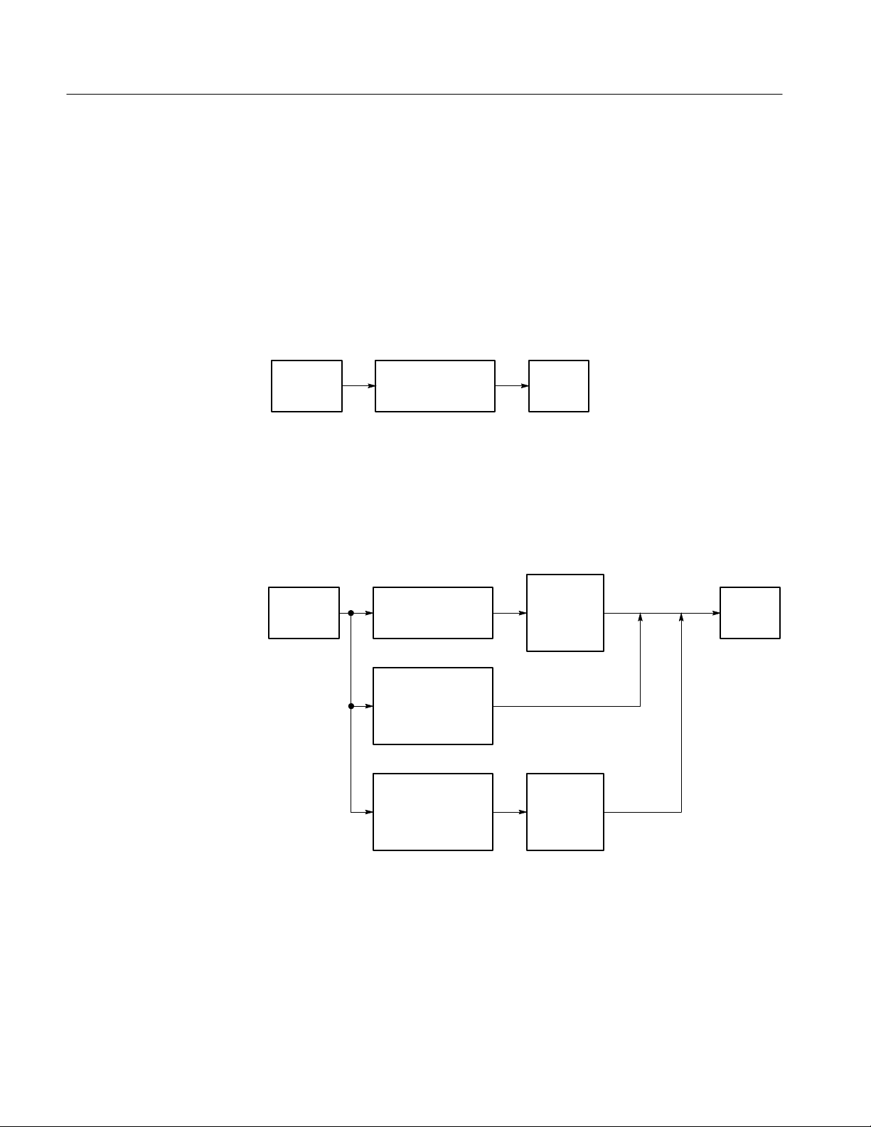
Functional Overview
Delayed Triggering
The waveform analyzer provides delayed trigger functionality with the delay
capabilities of TRIGger:A and TRIGger:B. TRIGger:A provides a time delay
and TRIGger:B provides a delay by number of edge events and by a time delay.
The time delay specifies a period to wait after the trigger event to start
acquisition.
There are two ways to delay the acquisition of waveforms: delayed runs after
main and delayed triggerable. Delayed triggerable uses the TRIGger:B system.
Delayed runs after main looks for a TRIGger:A event, then waits a user-defined
time, and then starts acquiring. See Figure 2–14.
Wait for
TRIGger:A
Wait User-specified
time
Acquire
Waveform
Figure 2–14: Delayed runs after main
Delayed triggerable mode looks for a TRIGger:A event and then, makes one of
the three types of delayed triggerable acquisitions. Figure 2–15 shows the
delayed trigger modes and the sequence for each delayed mode.
Delayed triggerable
after time
Delayed triggerable
after events
Delayed triggerable
after events/time
Wait for
TRIGger:A
event
Wait User-specified
time
Wait the
User-specified
number of TRIGger:B
events
Wait the
User-specified
number of TRIGger:B
events
Wait for
Trigger:B
event
Wait
User-specified
time
Acquire
Waveform
Figure 2–15: Delayed triggerable
Figure 2–16 shows the traditional delayed trigger modes and the commands used
to set these modes.
2–26
TVS600 Series Waveform Analyzers User Manual
Page 67

Functional Overview
Delayed runs after main
Trigger A
source
Delayed triggerable by events
Trigger A
source
Trigger B
source
Delayed triggerable by time
Indicates
trigger points
Time delay
(TRIGger:DELay)
Waiting for nth event
(where n=5)
(TRIGger:B:ECOunt)
Pretrigger
samples
Waveform record
Start posttrigger acquisition
Waveform record
Start posttrigger acquisition
Waveform record
Posttrigger
samples
Trigger A
source
Trigger B
source
Delayed triggerable by events and time
Trigger A
source
Trigger B
source
Waiting for nth event
(where n=4)
(TRIGger:B:ECOunt)
Figure 2–16: How the delayed triggers work
Time delay
(TRIGger:DELay)
Trigger B time delay
(TRIGger:B:DELay)
Start posttrigger acquisition
(first trigger after delay)
Waveform record
Start posttrigger acquisition
TVS600 Series Waveform Analyzers User Manual
2–27
Page 68

Functional Overview
Interaction Between Delay and Holdoff. Trigger delay determines how long after a
trigger event to start acquisition. Trigger holdoff sets how long after one trigger
another event another can occur. Figure 2–17 shows the relationship between
trigger delay and trigger holdoff. Note that trigger holdoff must include the
trigger delay time to be effective.
Trigger delay time
(TRIGger:DELay:TIME)
Trigger level
Indicates
trigger points
Waveform
record
Waveform
record
Trigger delay timeTrigger delay time
Waveform
record
Pulse Triggering
Holdoff
(TRIGger:HOLDoff:TIME)
Triggers are not recognized during holdoff time.
Holdoff
Holdoff
Figure 2–17: Trigger holdoff time with trigger delay time
The waveform analyzer can trigger on various pulse types using a special set of
TRIGger:PULSe parameters. When a qualified pulse event occurs, acquisition is
started just as it would from an edge trigger. Use the TRIGger[:A]:TYPE
command to select pulse triggering.
There are two classes of pulse triggering available, which you select with the
command TRIGger:PULSe:CLASs. The classes of PULSe triggering are as
follows:
H GLITch triggering occurs when the trigger source detects a pulse narrower
(or wider) in width than some specified time. It can trigger on glitches of
either polarity.
H WIDTh triggering occurs when the trigger source detects a pulse that is
inside or, optionally, outside some specified time range (defined by the upper
limit and lower limit). The waveform analyzer can trigger on positive or
negative width pulses.
2–28
Figure 2–18 shows the PULSe trigger parameters and the commands used to set
GLITch and WIDTh parameters. Both classes of PULSe triggering have unique
parameters except for the vertical level parameter, TRIGger:PULSe:THReshold,
which they share. THReshold determines the width of a pulse which is then
compared against qualifying parameters.
TVS600 Series Waveform Analyzers User Manual
Page 69

Glitch triggering
(TRIGger:PULSe:CLASs:GLITch)
TRIGger:PULSe:THReshold
TRIGger:PULSe:GLITch:POLarity
(positive, negative or either)
Width triggering
(TRIGger:PULSe:CLASs:WIDTh)
Functional Overview
Measured
pulse width
Measured pulse width is compared
against TRIGger:PULSe:GLITch:WIDth.
Select > or < comparison with
TRIGger:PULSe:GLITch:QUALify.
TRIGger:PULSe:WIDTh:HLIMit
TRIGger:PULSe:WIDTh:LLIMit
TRIGger:PULSe:THReshold
TRIGger:PULSe:WIDTh:POLarity
(positive or negative)
Select INside or OUTside
transition qualification with
TRIGger:PULSe:WIDTh:
QUALify.
Figure 2–18: Parameters for pulse triggering
The qualifying parameters for GLITch triggering are as follows:
H POLarity sets what pulse polarity can qualify the trigger event. The choices
are POSitive, NEGative, or BOTH. The selection BOTH accepts either
positive or negative pulses.
H WIDth sets the comparison pulse width used to qualify the measured pulse
width. The THReshold level helps determine the measured pulse.
H QUALify sets whether the measured width must be greater than (GT) or less
than (LT) the WIDth parameter to generate a trigger event.
TVS600 Series Waveform Analyzers User Manual
2–29
Page 70

Functional Overview
The qualifying parameters for WIDTh triggering are as follows:
H POLarity sets what pulse polarity can qualify the trigger event. The choices
are POSitive or NEGative.
H WIDth:HLIMit sets the maximum extent of the range used to qualify the
measured pulse width. The THReshold level helps determine the measured
pulse.
H WIDth:LLIMit sets the minimum extent of the range used to qualify the
measured pulse width. The THReshold level helps determine the measured
pulse.
H QUALify sets whether the last edge of the pulse must be INside or OUTside
the region defined by the WIDth parameters to generate a trigger event.
VXIbus Triggering
The waveform analyzer can trigger on the VXI bus TTL and ECL trigger lines.
These are digital signals carried by the P2 backplane. They may be generated by
any VXIbus module, including the waveform analyzer. These lines provide an
easy way to trigger several modules from one VXI source. The TTLTrg lines
have a 12.5 Mhz clock speed and the ECLTrg lines 62.5 Mhz. No coupling or
filtering is possible due to the digital nature of these signals.
Use the command TRIGger:[A]:SOURce to select from the signals TTLTrg0 to
TTLTrg7 and ECLTrg0 to ECLTrg1. The TTL signals conform to the TTL logic
standard. Likewise, the ECL signals conform to the ECL logic standards.
The waveform analyzer can source the TTLTrg lines with any valid trigger
source. Use the commands OUTPut:TTLTrg and OUTPut:ECLTrg to configure
and drive the VXI trigger lines. For more information, refer to the
OUTPut:TTLTrg commands starting on page 3–144.
2–30
TVS600 Series Waveform Analyzers User Manual
Page 71

Calculations
Functional Overview
This section describes the waveform analyzer CALCulation subsystem. The
CALCulate subsystem provides an extensive set of measurement, mathematical,
transformation and filtering functions. This section begins with a discussion of
the two models or methods of programming the CALCulate subsystem. Then,
each of the following types of calculation is discussed:
H Measurements of signal parameters, such as rise time
H Waveform mathematics for inverting, adding, subtracting, and multiplying
waveform records
H Waveform Integration, which creates the integral of a waveform record (see
page 2–39)
H Waveform Differentiation, which creates the derivative of a waveform record
(see page 2–39)
H Fast Fourier Transforms (FFT) which produce an amplitude versus frequency
waveform record (see page 2–40)
Overview of CALC Models
H Digital filtering used to remove certain frequency components from a
waveform record
The calculation system provides two methods for defining calculations:
H With the standard SCPI model, you define a signal source and a series of
functions to execute on the source.
H With the expression model you describe a calculation with an algebraic
expression using signal sources as variables.
Only one of the two CALC models may be active at a time. Both models allow
you to use all CALC functions, such as FILTer and TRANsform. The expression
model also allows calculations that operate on more than one source at a time,
such as when adding the waveforms in CH 1 and CH 2. In general, the SCPI
model allows only calculations that operate on one source at a time. (Measurement calculations using two waveforms, such as phase or delay, are exceptions to
the one source limitation.) The two models are discussed in detail under the
topics SCPI Calculation Model and Expression Calculation Model in this section.
Four CALC Blocks. The waveform analyzer provides four separate CALC blocks,
each with separately defined CALC settings. This means that for each CALC
block you will use you must set the measurement parameters in each CALC
block or accept the default settings. For example, to perform the same measurement on the CH 1 and CH 2 inputs, you first define the measurement in two
CALC blocks with a command like the following command:
TVS600 Series Waveform Analyzers User Manual
2–31
Page 72

Functional Overview
CALC1:WML FTIM,RTIM;:CALC2:WML FTIM,RTIM
Two CALC blocks can perform measurements on the same source. This feature
allows you to perform a calculation, such as a measurement, in more than one
way for every acquisition. For example, you could perform the same measurement in two CALC blocks, but use the FILTer function to remove high-frequency
components from the waveform before the measurement in one of the CALC
blocks.
For information on setting parameters for calculation functions, refer to the
individual command descriptions in section 3 and to discussions of the CALC
functions in this section of the manual.
SCPI Calculation Model
The waveform analyzer supports the standard SCPI calculation model. In the
SCPI CALCulate model, you use the CALCulate:PATH command to define a
series of functions to perform on a single source. Figure 2–19 shows how the
CALC:PATH command sets the data flow through a set of functions.
CALCulate:PATH (function 1), (function 2), (function 3), . . . (function n)
*(STATe OFF)
Data source: CALCulate1:FEED1
Example of setting a function: FILTER:STATe On or Off
Function 1 Function 3
*
Function is ignored if STATe is OFF
Function 2
Figure 2–19: P ATH definition for SCPI calculation model
Functions included in the CALC:PATH are performed only when their individual
STATe is set to ON. Functions whose STATe is set to OFF are not executed and
any data passed to them is routed unchanged to the next function in the PATH.
*(STATe OFF)
*(STATe OFF)*(STATe OFF)
Function n
2–32
When defining SCPI model calculations that measure parameters based on two
waveforms (such as Gain and Delay), the functions you set using CALC:PATH
only apply to the data source selected with FEED1. The source selected by
FEED2 is unaffected by the functions you select.
NOTE. SCPI model calculations are disabled when you define an expression
model calculation with CALC:PATH:EXPR.
TVS600 Series Waveform Analyzers User Manual
Page 73

Functional Overview
CALC Data Source. You must define a single data source for each CALC block
using the CALC:FEED1 command. See Figure 2–19. The allowed sources are
the function strings “XTIM:VOLT <n>” that represent the input channels. The
command CALC1:FEED1 “XTIM:VOLT 1” connects the CH 1 waveform record
to the CALC1 block. You may also specify the FEED1 source as CHAN<n>.
More than one CALC block can operate on a source. For more information, refer
to the CALC:FEED1 command in section 3 of this manual.
You may also define a second data source for each CALC block using the
CALC:FEED2 command. The allowed sources are the same as for
CALC:FEED1; for example, the command CALC1:FEED2 “XTIM:VOLT 2”
connects the CH 2 waveform record to the CALC1 block. SCPI-model calculations that make dual-waveform measurements (such as when measuring Gain or
Delay) can make use of the second data source.
Expression Model
The waveform analyzer supports an expression based model for defining
calculations. With the expression model, you define a calculation involving one
or more functions using an algebraic expression. The expression syntax follows
standard C language syntax. For example, the following expression calculates the
derivative of the difference between the CH 1 and CH 2 input signals.
CALC1:PATH:EXPR (DER(CHAN1-CHAN2))
The source to operate on is defined in the expression (CHAN1 and CHAN2 in
the example) and not with a FEED command as in the SCPI model. The sources
must be in acquisition memory to provide the expression with useful data. If
CHAN 1 is not acquired, the above expression would produce an error during
acquisition and calculation.
EXPRession Syntax. The syntax for CALCulate expressions is defined in the
following BNF description:
<expr> ::= <factor> {[+|-|*|/] <factor>}
<factor> ::= [-<number>|{+}<number>]
|<ch_expr>
|AATS
|<func>"("<expr>[,<expr>]")"
<ch_expr> ::= <chan>{"["<nrx>"]"}
<chan> ::= [WMP1:|WMP2:|WMP3:|WMP4:]
CHAN1|CHAN2|CHAN3|CHAN4
<func> ::= AAMLIST|AC|AMPLitude|AREA|CARea|CMEan|
CRMS|CROss|DC|DELay|DERivative|FFT|
FILTer|FORMat|FREQuency|FTIMe|GAIN|HIGH|
INTegral|LOW|MAXimum|MEAN|MID|MINimum|
NCRoss|NDUTycycle|NWIDth|PCRoss|PERiod|
TVS600 Series Waveform Analyzers User Manual
2–33
Page 74

Functional Overview
PHAse|PWIDth|PTPeak|RMS|RTIMe|
SDEViation|SMOothing|TRANsform|TTRig|
WMList]
An example of the expression syntax follows:
CALC1:PATH:EXPR (FORM(TRAN(FILT(CHAN1))))
This command performs frequency filtering on CHAN1, then performs an FFT
transform and finally formats the result, perhaps in a logarithmic magnitude
format. The settings for CALC:FILTer, :TRANsform, and :FORMat functions
must be completed in separate command statements prior to starting acquisition.
The settings might include enabling the low pass filter with
CALC:FILT:FREQ:LPAS, setting the TRANsform WINDow type, and setting
the result format for the resulting FFT waveform record with CALC:FORM
MLOG.
The following example produces a waveform composed of data points that are
the ratio of the deviation from the MEAN over the measured AMPLitude.
Measurements
CALC2:PATH:EXPR ((CHAN1-MEAN(CHAN1))/AMPL(CHAN1))
Expressions for Auto-Advance Records. Expressions for auto-advance acquisition
are similar to those for normal acquisition. You can specify a set of measurements to perform on all auto-advance waveform records with the command
CALC1:AAMList. An example follows:
CALC1:PATH:EXPR (AAMList(CHAN1))
If AAMList is set to measure RTIMe (rise time), the expression returns a vector
of RTIMe measurements for all auto-advance acquisitions (as delimited by
AADV:REC:START,COUNT).
You can also specify individual measurements or functions to perform on a single
record. In the following example, MEAN is measured only on auto-advance
record number five.
CALC1:PATH:EXPR (MEAN(CHAN1[5]))
The waveform analyzer provides voltage, time, area, and statistical waveform
measurements. This section describes these measurements and how to use them.
For algorithm information, see Appendix B: Algorithms.
2–34
Table 2–2 lists the available measurements in the waveform analyzer.
TVS600 Series Waveform Analyzers User Manual
Page 75

T able 2–2: Measurement Definitions
Measurement Command Definition
AMPLitude Voltage measurement. The High value less the Low value measured over the entire waveform.
This result is not usually equal to the peak-to-peak value because of the way High and Low are
determined.
AREA Voltage over time measurement. The area over the entire waveform in volt-seconds. Area
measured above ground is positive; area below ground is negative.
CARea (Cycle area) Voltage over time measurement. The area over the first cycle in the waveform in volt-seconds.
Area measured above ground is positive; area below ground is negative.
CMEan (Cycle mean) Voltage measurement. The arithmetic mean over the first cycle in the waveform.
CRMS (Cycle RMS) Voltage measurement. The true Root Mean Square voltage over the first cycle in the waveform.
CROSs Timing measurement. The time of the Nth positive- or negative-going crossing of the MREF
(mid-reference) level, where N is set by CALC<n>:WMP:EDGE. Time is relative the trigger point
of the acquisition.
DELay Timing measurement. The time between the MidRef crossings of a reference and a target
waveform.
FREQuency Timing measurement for the first cycle in the waveform. The reciprocal of the PERiod. Measured
in Hertz (Hz).
FTIMe (Fall time) T iming measurement. Time taken for the falling edge of the first pulse in the waveform to fall from
a HREF value (default = 90%) to a LREF value (default =10%) of its final value.
GAIN Ratio measurement. An amplitude measurement of a target waveform is divided by an amplitude
measurement of a reference waveform.
HIGH The value used as 100% whenever HREF, MREF, and LREF values are needed (as in fall time and
rise time measurements). Set to absolute value or calculated as the peak value or histogram, which
finds the most common value. See Methods of Setting HIGH and LOW on page 2–38.
LOW The value used as 0% whenever HREF, MREF, and LREF values are needed (as in fall time and
rise time measurements). Set to absolute value or cal culated as the peak value or histogram, whi ch
finds the most common value. See Methods of Setting HIGH and LOW on page 2–38.
MAXimum Voltage measurement. The most positive peak voltage measured over the entire waveform.
Functional Overview
AMPLitude = HIGH – LOW
MEAN or DC Voltage measurement. The arithmetic mean over the entire waveform. Use MEAN or DC to select
this measurement.
MID The value half way between MAXimum and MINimum values. Units are in current vertical units.
MID +
MINimum Voltage measurement. The most negative peak voltage measured over the entire waveform.
NCROSs Timing measurement. The time of the Nth negative-going crossing of the MREF (mid-reference)
level, where N is set by CALC<n>:WMP:EDGE. Time is relative the trigger point of the
acquisition.
TVS600 Series Waveform Analyzers User Manual
MAXimum – MINimum
2
2–35
Page 76

Functional Overview
T able 2–2: Measurement Definitions (Cont.)
Measurement Command Definition
NDUT ycycle
(Negative Duty Cycle)
NWIDth (Negative Width) Timing measurement of the first pulse in the waveform. The distance (time) between MREF
PERiod Timing measurement. Time for the first complete signal cycle to complete in the waveform. The
PDUT ycycle
(Positive Duty Cycle)
PCROSs Timing measurement. The time of the Nth positive–going crossing of the MREF (mid-reference)
Phase Timing measurement. The amount one waveform leads or lags another in time. Expressed in
PTPeak (Peak to Peak) Voltage measurement. The absolute difference between the MAXimum and MINimum amplitude
PWIDth (Positive Width) Timing measurement of the first pulse in the waveform. The distance (time) between MREF
RMS or AC Voltage measurement. The true Root Mean Square voltage over the entire waveform. Use RMS
RTIMe (Rise time) Timing measurement. Time for the leading edge of the first pulse to rise from the LREF value
SDEViation
(Standard deviation)
TTRIG Timing measurement. The time difference between the main and the delay triggers. Value
Timing measurement of the first cycle in the waveform. The ratio of the negative pulse width to
the signal period, expressed as a percentage.
NDUTycycle +
(default 50%) amplitude points of a negative pulse.
reciprocal of frequency . Measured in seconds.
Timing measurement of the first cycle in the waveform. The ratio of the positive pulse width to the
signal period, expressed as a percentage.
PDUTycycle +
level, where N is set by CALC<n>:WMP:EDGE. Time is relative the trigger point of the
acquisition.
degrees, where 360_ comprise one waveform cycle.
in the entire waveform.
(default 50%) amplitude points of a positive pulse.
or AC to select this measurement.
(default = 10%) to the HREF value (default = 90%).
Deviation from the MEAN measurement. The square root of the arithmetic mean of the squares
of each measurement deviation from the measured MEAN. Result is in current vertical units.
returned is independent of channel number. Value returned is valid only when the delay trigger
source is not set to immediate.
NegativeWidth
Period
PositiveWidth
Period
100%
100%
Measurement Parameters
2–36
You can specify measurements to perform using either the SCPI model or the
expression model. The models are discussed starting on page 2–32. The
parameters used to make measurements are listed in Table 2–3.
The automated measurements have parameters, such as LREF, MREF, and
HREF, that determine how to make the various measurements. You can set the
parameters with the CALCulate:WMParameter commands or use their default
values. Table 2–3 lists the measurement parameters along with a description of
TVS600 Series Waveform Analyzers User Manual
Page 77

Functional Overview
each. Following the table are discussions on the methods of setting parameters
such as absolute or relative reference levels.
T able 2–3: Measurement Parameters
Reset
Measurement Parameter
EDGE 1 Sets the edge(s) used for cross, ncross, pcross, and
HIGH 0.0 Sets the high or most positive level in current vertical
LOW 0.0 Sets the low or most minimal level in current vertical
HREFerence 0.0 Sets the high reference or distal level in current vertical
HREFerence:RELative 0.9 (90%) Sets the high reference or distal level as a percentage
LREFerence 0.0 Sets the low reference or proximal level in current
LREFerence:RELative 0.1 (10%) Sets the low reference or proximal level as a
MREFerence 0.0 Sets the middle reference or mesial level in current
MREFerence:HYSTeresis 0.05 (5%) Sets the hysteresis value as a percentage of the
MREFerence:RELative 0.5 (50%) Sets the middle reference or mesial level as a
SLOPe POS Sets the direction, positive- or negative-going, of the
Value
Description
delay measurements.
units. Used for amplitude and time measurements
when CALC:WMP:HMEThod is set to ABSolute.
units. Used for amplitude and time measurements
when CALC:WMP:LMEThod is set to ABSolute.
units. Used for rise time (RTIM) and fall time (FTIM)
measurements when CALC:WMP:RMEThod is set to
ABSolute.
of the current value for HIGH. Used for rise time (RTIM)
and fall time (FTIM) measurements when
CALC:WMP:RMEThod is set to RELative.
vertical units. Used for rise time (RTIM) and fall time
(FTIM) measurements when CALC:WMP:RMEThod is
set to ABSolute.
percentage of the current value for HIGH. Used for rise
time (RTIM) and fall time (FTIM) measurements when
CALC:WMP:RMEThod is set to RELative.
vertical units. Used for timing measurements when
CALC:WMP:RMEThod is set to ABSolute.
current value for AMPLitude. Reduces effects of noise
on measurements.
percentage of the current value for HIGH. Used for
timing measurements when CALC:WMP:RMEThod is
set to RELative.
edge(s) used for cross and delay measurements.
TVS600 Series Waveform Analyzers User Manual
2–37
Page 78

Functional Overview
Methods of Setting HIGH and LOW. The waveform analyzer provides four ways to
setting the reference levels HIGH and LOW which are used in many amplitude
and time measurements. The methods are as follows:
ABSolute — specifies that HIGH and LOW are set to absolute amplitude
levels with CALCulate:WMParameter:HIGH and :LOW.
AUTO — selects the MODE method of setting HIGH and LOW when the
histogram function is able to detect a consistent level above and below MID.
Otherwise, the PEAK method is used. AUTO method is effective when you
are not certain what type of waveform to expect.
MODE — selects the levels for HIGH and LOW based on a peak histogram
function which looks for the most common value above and below MID.
This method ignores short term aberrations, such as overshoot and ringing,
on a digital logic waveform.
PEAK — specifies that HIGH and LOW are set to the highest and lowest
values in the waveform record. This method is useful for a sinewave or
triangle waveform but not for digital pulses.
Waveform Math
You can choose to set HIGH and LOW using different methods. For more
information on setting HIGH and LOW, refer to Appendix B: Algorithms.
Methods of Setting Reference Levels. Two methods are available for setting the
reference levels LREF, MREF, and HREF. The methods are ABSolute and
RELative which you pick with the command CALC:WMP:RMEThod. ABSolute
lets you set the reference levels as absolute vertical levels. RELative lets you set
them as a ratio or percentage of the value for the measurement parameter HIGH.
For more information on setting reference levels, refer to Appendix B: Algo-
rithms.
The waveform analyzer provides a means to mathematically manipulate your
waveforms. You can add (+), subtract (–), multiply (*) or divide (/) two
waveforms or a waveform and a scalar. The scalar can be the result of another
measurement such as MEAN in the following example:
CALC1:PATH:EXPR (CHAN1 - (MEAN (CHAN1)))
All other CALC functions are compatible with the math operators. You can use
the minus operator (–) to negate a scalar value. For more information on
expression syntax, refer to Expression Model on page 2–33.
2–38
TVS600 Series Waveform Analyzers User Manual
Page 79

Functional Overview
Waveform Differentiation
The calculation capabilities of the waveform analyzer include waveform
differentiation. This capability allows you to compute a derivative math
waveform that indicates the instantaneous rate of change of the waveform
acquired. Derivative waveforms are useful in the measurement of the slew rate of
amplifiers.
Use the command CALC<n>:DERivative:STATe to enable differentiation for a
particular CALC block. For example, when CALC2:DER:STATe is ON, the
CALC2 block will perform differentiation on the CALC2 source.
The resultant waveform is referred to as CALC<n> where <n> is the CALC
block that performed the differentiation. Each of the four CALC blocks can
perform differentiation when enabled. Use TRACe? CALC<n> to retrieve the
resultant waveform.
The math waveform, derived from the sampled waveform, is computed based on
the following equation:
Yn+ (X
Where: X is the source waveform
Since the resultant math waveform is a derivative waveform, its vertical units are
volts/second (its horizontal units are seconds). The source signal is differentiated
over its entire record length; therefore, the math waveform record length equals
that of the source waveform.
(n)1)
1
* Xn)
T
Y is the derivative math waveform
T is the time between samples
Waveform Integration
TVS600 Series Waveform Analyzers User Manual
The calculation capabilities of the waveform analyzer include waveform
integration. This capability allows you to compute an integral math waveform
that is an integrated version of the acquired waveform.
Use the command CALC<n>:INTegral:STATe to enable integration for a
particular CALC block. For example, when CALC2:INT:STATe is ON, the
CALC2 block will perform integration on the CALC2 source.
The resultant waveform is referred to as CALC<n> where <n> is the CALC
block that performed the calculation. Each of the four CALC blocks can perform
integration when enabled. Use TRACe? CALC<n> to retrieve the resultant
waveform record.
The integral waveform record, derived from the sampled waveform, is computed
based on the following equation:
y(n) + scale
n
x(i) ) x(i * 1)
i + 1
2
T
2–39
Page 80

Functional Overview
Where: x(i) is the source waveform
y(n) is a point in the integral waveform
scale is the output scale factor
T is the time between samples (sample interval)
Since the resultant waveform record is an integral waveform, its vertical units are
volt-seconds (its horizontal units are seconds). The source signal is integrated
over its entire record length; therefore, the waveform record length equals that of
the source waveform.
Transforms (FFT)
The calculation capabilities of the waveform analyzer include taking the Fast
Fourier Transform (FFT) of a waveform record. The FFT allows you to
transform an amplitude versus time waveform into one that plots the amplitudes
of the various discrete frequencies the waveform contains.
The FFT computes the frequency content of a waveform you specify as a CALC
block source. The transform of the source waveform is based on the following
equation:
N–1
X(k) +
Where: x(n) is a point in the time domain record
The resulting waveform is a record consisting of N/2 complex coefficients
representing values in the frequency domain. The horizontal scale for FFT
waveforms is expressed in frequency with the first point of the waveform record
representing zero frequency (DC).
1
N
S
n + 0
X(k) is a point in the frequency domain record
n is the index to the time domain record
k is the index to the frequency domain record
N is the length of the time domain record
j is the square root of −1
x(n)e
j2pnk
–
N
for : k + 0to
N
2
2–40
Setting the Record Format. You can convert the complex data in the resultant
transform record into magnitude or phase data using the CALC:FORMat
function. The following lines set the waveform analyzer to perform a TRANsform on CH 1 and format the result as phase data:
CALC1:FORM PHAS
CALC1:PATH:EXPR (FORM(TRAN(CHAN1)))
TVS600 Series Waveform Analyzers User Manual
Page 81
Functional Overview
Zero Phase Reference Point. The zero phase reference point for an FFT phase
waveform is in the middle of the FFT time domain record regardless of the
waveform record length. Figure 2–20 shows this placement.
FFT Frequency Domain Record
Waveform Record
Zero Phase
Reference
Figure 2–20: Zero phase reference point in FFT phase records
FFT Frequency Range and Resolution. The waveform analyzer can return either
the magnitude or phase angle of the FFT frequency domain record. The
resolution between the discrete frequencies in this waveform is determined by the
following equation:
Sample Rate
DF +
Input Length
Where:
DF is the frequency resolution.
Sample Rate is the sample rate of the source waveform.
Input Length is the length of the source waveform record.
The sample rate also determines the range these frequencies span; they span from
1
0 to
the sample rate of the waveform record. (The value of
2
1
the sample rate is
2
often referred to as the Nyquist frequency or point.) For example, a sample rate
of 20 Megasamples per second would yield an FFT with a range of 0 to 10 MHz.
Undersampling (Aliasing). Aliasing occurs when the waveform analyzer acquires a
source waveform with frequency components outside of the frequency range for
the current sample rate. In an FFT waveform record, the actual higher frequency
components are undersampled, and therefore, they appear as lower frequency
aliases that “fold back” around the Nyquist point
(1
the sample rate). See
2
Figure 2–21.
H Source waveforms with fast edge transition times create many high
frequency harmonics. These harmonics typically decrease in amplitude as
their frequency increases.
H Sample the source signal at rates that are at least 2X that of the highest
frequency component having significant amplitude.
TVS600 Series Waveform Analyzers User Manual
2–41
Page 82

Functional Overview
H If necessary, filter the input to limit its bandwidth to frequencies below the
Nyquist frequency.
Nyquist Frequency
Point
Frequency
Actual FrequenciesAliased Frequencies
Figure 2–21: How aliased frequencies corrupt an FFT transform
FFT Windows. An FFT window acts like a bandpass filter between the time
domain record and the FFT frequency domain record. The shape of the window
controls the ability of the FFT to resolve (separate) frequencies and to accurately
measure the amplitude of those frequencies. Figure 2–22 shows how a window is
used in the transform process.
You can select from six windows for the transform with the command
CALC:TRAN:FREQ:WIND. Each window provides benefits and losses. For
example, if you select a window to provide better frequency resolution you give
up a degree of amplitude accuracy. In general, choose a window that can just
resolve the frequencies you want to measure. The available windows and their
characteristics are as follows:
RECTangular — Best type for resolving a narrow band of frequencies but
worst for accurate amplitude of those frequencies. Good for measuring
nonrepetitive signals and frequency components near DC.
HAMMing — Very good window for resolving frequencies that are very
close to the same value with somewhat improved amplitude accuracy over
the rectangular window.
HANNing — Very good window for measuring amplitude accuracy but
degraded for resolving frequencies.
2–42
BHARris — Widest bandwidth and lowest side lobes. Best for viewing a
broad spectrum.
TVS600 Series Waveform Analyzers User Manual
Page 83

Functional Overview
BLACkman — Best window for measuring the amplitude of frequencies but
worst at resolving frequencies.
TRIangular — Window with the least attenuation of side lobes.
Source Waveform Record
Xs
FFT Window
Source Waveform Record
After Windowing
FFT
FFT Frequency Domain
Record
Figure 2–22: Windowing the FFT time domain record
Figure 2–23 shows each window, its bandpass characteristic, bandwidth, and
highest side lobe. When choosing a window, consider the following
characteristics:
H The narrower the central lobe for a given window, the better it can resolve a
frequency.
H The lower the lobes on the side of each central lobe are, the better the
amplitude accuracy of the frequency measured in the FFT using that window.
H Hamming, Hanning, Blackman, and BHarris are all bell-shaped windows that
taper the waveform record at the ends. The Hanning and BHarris windows
taper the data at the end of the record to zero; therefore, they are generally
TVS600 Series Waveform Analyzers User Manual
2–43
Page 84

Functional Overview
better choices to eliminate leakage. However, be certain to position the most
interesting parts of the signal in the center region of the waveform record.
H If the Hanning window merges frequencies, try the Hamming window before
settling on the rectangular window. Depending on the distance of the
frequencies you are trying to measure from the fundamental, the Hamming
window sometimes resolves frequencies better than the Hanning.
2–44
TVS600 Series Waveform Analyzers User Manual
Page 85

Functional Overview
FFT Window Type Bandpass Filter
Rectangular Window
Hamming Window
Hanning Window
Blackman Window
–3 dB Bandwidth Highest Side Lobe
0 dB
-20
-40
-50
0 dB
-20
0.89
1.30
-40
-60
0 dB
-20
-40
-60
-80
0 dB
-20
-40
-60
-80
1.44
1.68 –58 dB
–13 dB
–43 dB
–32 dB
0 dB
-20
BHarris Window
Triangle Window
-40
-60
-80
-100
-101
0 dB
-20
-40
-60
-80
1.90 –92 dB
1.28 –27 dB
Figure 2–23: FFT windows and bandpass characteristics
Leakage. Leakage results when the time domain waveform delivered to the
TRANsform (FFT) function contains a non-integer number of waveform cycles.
Since there are fractions of cycles in such records, there are discontinuities at the
ends of the record. These discontinuities cause energy from each discrete
TVS600 Series Waveform Analyzers User Manual
2–45
Page 86

Functional Overview
frequency to “leak” over on to adjacent frequencies. The result is amplitude error
when measuring those frequencies.
Digital Filtering
The waveform analyzer provides a configurable digital filter to perform
post-acquisition frequency filtering. There are four types of filters available:
BPASs — rejects frequencies outside the defined frequency range.
HPASs — rejects frequencies below the defined frequency range.
LPASS — rejects frequencies above the defined frequency range.
NOTCh — rejects frequencies within the defined frequency range.
Use the command CALC:FILT:FREQ[:TYPE] to select a digital filter. Once you
have selected a filter and configured it (see the following discussion) you must
enable the filter with CALC:FILT:FREQ:STATe when using the standard
SCPI model.
Filter Parameters. Each digital filter function has a set of parameters that
determine its effective frequency range and roll off. The LPAS and HPASs filters
have specific cutoff parameters. Other parameters affect the roll off or transition
region. Figure 2–24 shows the main parameters that control the four digital filters
and the commands used to set them. Note that the parameters set the –6dB point
of attenuation.
The NOTCh and BPASs bandpass filters are set with either of two command
pairs: CENTer and SPAN or STARt and STOP. Figure 2–25 shows how these
command pairs effectively control the same parameters. Setting a parameter of
one pair affects the settings of the other pair. For example, if you could set the
BPAS filter parameter STARt to 50 MHz and STOP to 100 MHz using the
following command.
2–46
CALC1:FILT:FREQ BPAS; FREQ:STAR 50E6; STOP 100E6
A query of CENTer and SPAN will return 75 MHz and 50 MHz, respectively. If
you then set SPAN to 100 MHz and leave CENTer at 75 MHz, the STARt value
changes to 25 MHz and the STOP value changes to 125 MHz. The new SPAN
value is spread on either side of CENTer requiring a change in the ends of the
pass band.
TVS600 Series Waveform Analyzers User Manual
Page 87

Low pass filter High pass filter
Functional Overview
Amplitude (dB)
0
–6
Frequency
Rejection band
Pass band
CALCulate:FILTer:FREQuency:LPASs
Amplitude (dB)
0
–6
Rejection band
CALCulate:FILTer:FREQuency:HPASs
Notch filter Bandpass filter
Amplitude (dB)
0
Amplitude (dB)
0
Frequency
Pass band
–6
Frequency
Pass
band
CALCulate:FILTer:FREQuency:STARt
Rejection
band
CALCulate:FILTer:FREQuency:STOP
Pass
band
Figure 2–24: Parameters for the four digital filters
–6
Rejection
band
CALCulate:FILTer:FREQuency:STARt
Pass band
CALCulate:FILTer:FREQuency:STOP
Frequency
Rejection
band
TVS600 Series Waveform Analyzers User Manual
2–47
Page 88

Functional Overview
Amplitude (dB)
0
–6
Frequency
CALCulate:FILTer:FREQuency:STARt
(Set frequency)
CALCulate:FILTer:FREQuency:STOP
(Set frequency)
Figure 2–25: Two methods of setting BPASs and NOTCh filters
Transition Settings. The roll off or transition region between the pass band and
the rejection band for all filter functions is controlled by the parameters
SREJection and TWIDth. Figure 2–26 shows these parameters. SREJection
controls the degree of attenuation and is specified in dB. The minimum setting is
15 dB and the maximum is 100 dB. TWIDth determines the rate of roll off or
transition width. TWIDth is specified as a value between 0 and 1 which is
derived using the following relation:
Amplitude (dB)
0
–6
Frequency
CALCulate:FILTer:FREQuency:CENTer
(Set frequency)
CALCulate:FILTer:FREQuency:SPAN
(Set frequency range)
TWIDth = Transition Frequency * 2 * SWEep:TINTerval
The transition frequency is the actual range of frequencies over which the filter
transitions from the pass band to the rejection band. SWEep:TINTerval is the
current sample interval. The smaller the value of TWIDth the smaller the
transition region and steeper the transition slope. To set TWIDth to 0.05 you
would use the command
CALC1:FILT:FREQ:TWID 0.05
2–48
TVS600 Series Waveform Analyzers User Manual
Page 89

Functional Overview
Amplitude (dB)
0
CALCulate:FILTer:FREQuency:SREJection
(Range –15 dB to –100 dB)
Frequency
CALCulate:FILTer:FREQuency:TWIDth (0 to 1.0)
Figure 2–26: Rejection level and transition slope for the digital filter
For more information on the digital filter, refer to the Filter discussion in
Appendix B, Algorithms.
TVS600 Series Waveform Analyzers User Manual
2–49
Page 90

Functional Overview
Fast Data Channel
The Fast Data Channel (FDC) provides a fast transfer protocol for moving
waveform records and other data between the waveform analyzer and a VXIbus
controller. The waveform analyzer includes an FDC driver that provides the
instrument side of the protocol.
The controller must initiate FDC transfers; therefore, you must ensure that your
controller has an FDC driver to communicate correctly with the waveform
analyzer FDC channel. Refer to your VXI system communications software
manual to learn how to initiate an FDC channel on your controller. See Note
below.
NOTE. The VXIplug&play VISA I/O interface provides FDC support. The
sections Fast Data Channel and Auto-Advance Acquisition on page 2–16
discusses setting up an FDC session using this interface. In particular, see
step 10 on page 2–18 of that section for use of the VISA commands to configure
the FDC session.
Table 2–4 lists the commands that control the instrument side of the FDC
protocol.
T able 2–4: Commands for Fast Data Channel and Associated Functions
Command Description
TRACe:COPY FDC1,<source> Copies waveform records or CALCulate block results to the
outgoing Fast Data Channel (FDC1). Y ou can specify one or
more sources in a comma separated list. One selection is
AA TS which specifies all auto-advance waveform records.
Alternatively, use TRAC:OUT:FDC to specify a list of items
to transfer then use TRAC:COPY,LIST to transfer all the list
of items.
TRACe:OUTput:FDC Defines a list of waveform records, calculations, and the
output of auto-advance acquisition to transfer with the FDC.
The following example command transfers CH 1 and CH 2 waveform records
plus the results of the CALC1 and CALC2 blocks. (The transfer occurs
immediately upon sending the command; it does not wait for acquisition or
calculations to complete.)
TRAC:COPY FDC1,CHAN1,CHAN2,CALC1,CALC2
2–50
TVS600 Series Waveform Analyzers User Manual
Page 91

Functional Overview
NOTE. Refer to Fast Data Channel and Auto-Advance Acquisition on page 2–16
for an example of setting the waveform analyzer for auto-advance acquisition
with FDC waveform transfers.
FDC Code Example
The following C-code example sets up an FDC channel, configures the TVS600,
transfers a 512-point waveform, and closes the FDC channel. The program
assumes the controller uses the VXI Plug&Play Interface to control the FDC
session; users of other interfaces supplying FDC support should modify the
program to support those interfaces.
The program simply exits if an error occurs. You should add statements to the
program so it closes all sessions before exiting the program after an error.
The transferred waveform data is stored in a buffer (waveformBuf) as binary
bytes characters. For a 512-point record, the received data includes 1024 bytes
plus a few bytes of header information. The example program ends with the
appropriate statements to close all sessions.
NOTE. This program was written in MicroSoft C QuickWin. It must be compiled
with Microsoft Visual C++ as a QuickWin application. It must be compiled
using the large memory model.
TVS600 Series Waveform Analyzers User Manual
2–51
Page 92

Functional Overview
#include <stdio.h>
#include <stdlib.h>
#include <string.h>
#include "c:\vxipnp\win\include\visa.h"
#define WAVEFORM_BUF_SIZE 2048 */Buffer sized for 512 pt record */
void main() {
ViStatus status; /* Return value from VISA.DLL functions */
ViSession visaRM; /* VISA resource manager session handle */
ViSession tvs600; /* Session handle for command channel */
ViSession fdc; /* Session handle for FDC channel */
ViChar tvs600Desc[256]; /* Descriptor used to address TVS600 */
ViChar waveformBuf[WAVEFORM_BUF_SIZE]; /* Local waveform memory */
ViUInt32 retCnt; /* Returns actual number of bytes transferred */
/****************************************************************/
/* */
/* Establish Communication with the TVS600 */
/* */
/****************************************************************/
/* Set the TVS600 descriptor */
/* Customized following line with the logical address of TVS600. */
/* The address here is 2. */
strcpy(tvs600Desc, "VXI::2::INSTR");
/* Open session with the VISA default resource manager */
status = viOpenDefaultRM(&visaRM);
if (status) return;
/* Open a session with the tvs600 to send ASCII commands */
status = viOpen(visaRM, tvs600Desc, VI_NULL, VI_NULL, &tvs600);
if (status != VI_SUCCESS) return;
/* Open a session with the tvs600 to receive FDC data */
status = viOpen(visaRM, tvs600Desc, VI_NULL, VI_NULL, &fdc);
if (status != VI_SUCCESS) return;
Example continued on following page.
2–52
TVS600 Series Waveform Analyzers User Manual
Page 93

Example continued from previous page
/****************************************************************/
/* */
/* Set up the FDC session attributes */
/* */
/****************************************************************/
/* Selects FDC channel 1. */
/* The TVS600 outputs data on FDC channel 1. */
status = viSetAttribute(fdc, VI_ATTR_FDC_CHNL, 1);
if (status != VI_SUCCESS) return;
/* The TVS600 uses a stream channel. A stream channel can */
/* send a series of waveforms more efficiently. */
status = viSetAttribute(fdc, VI_ATTR_FDC_MODE, VI_FDC_STREAM);
if (status != VI_SUCCESS) return;
/* Select the FDC protocol for this session */
status = viSetAttribute(fdc, VI_ATTR_IO_PROT, VI_FDC);
if (status != VI_SUCCESS) return;
Functional Overview
/* Set the FDC session timeout to 10 seconds */
status = viSetAttribute(fdc, VI_ATTR_TMO_VALUE, 10000);
if (status != VI_SUCCESS) return;
/****************************************************************/
/* */
/* Set up the TVS600 acquisition */
/* */
/****************************************************************/
/* Initialize the TVS600 to a known state */
if (viPrintf(tvs600, "ABORT\n") != VI_SUCCESS) return;
if (viPrintf(tvs600, "*RST\n") != VI_SUCCESS) return;
/* Set up channel 1 for the acquisition: */
/* Ch 1 50 ohm, 512 pts record, 100 MS/s, transfer Ch 1 only */
if (viPrintf(tvs600, "INP:IMP 50\n") != VI_SUCCESS) return;
if (viPrintf(tvs600, "VOLT1:RANG 0.5\n") != VI_SUCCESS) return;
if (viPrintf(tvs600, "FUNC:ON CHAN1\n") != VI_SUCCESS) return;
if (viPrintf(tvs600, "FUNC:OFF CHAN2\n") != VI_SUCCESS) return;
if (viPrintf(tvs600, "DATA:LIST CHAN1\n") != VI_SUCCESS) return;
if (viPrintf(tvs600, "SWE:POIN 512\n") != VI_SUCCESS) return;
if (viPrintf(tvs600, "SWE:TINT 10nS\n") != VI_SUCCESS) return;
if (viPrintf(tvs600, "INIT\n") != VI_SUCCESS) return;
Example continues on following page
TVS600 Series Waveform Analyzers User Manual
2–53
Page 94

Functional Overview
Example continued from previous page
/****************************************************************/
/* */
/* Start transfer of TVS600 acquired data using FDC. */
/* */
/****************************************************************/
status = viRead(fdc, waveformBuf, WAVEFORM_BUF_SIZE, &retCnt);
if (status != VI_SUCCESS) return;
/****************************************************************/
/* */
/* Close all sessions to deallocate resources and memory */
/* */
/****************************************************************/
/* Close the command session */
status = viClose(tvs600);
if (status != VI_SUCCESS) return;
/* Close the FDC session */
status = viClose(fdc);
if (status != VI_SUCCESS) return;
/* Close the VISA resource manager */
status = viClose(visaRM);
if (status != VI_SUCCESS) return;
}
2–54
TVS600 Series Waveform Analyzers User Manual
Page 95

Data Transfer Formats
Functional Overview
The waveform analyzer allows you to set the format of transferred data.
Acquired data can be in ASCII integer or 16 bit binary formats. CALC data is
always floating point, but may be ASCII or 32 REAL type. The primary format
commands are in the FORMat subsystem.
The defined binary formats send the high byte (most significant) followed by
lower bytes by default. You can change the byte order with FORMat:BORDer to
either NORM (high byte/low byte) or SWAP (low byte/high byte).
Acquired Data Formats
The waveform analyzer uses signed, 16-bit integers to represent each data point
in a waveform record. The waveform data are transferred as either decimal
ASCII integers (ASCII,0) or 16 bit binary numbers (INT,16). You choose a
format with the FORMat command. Data values range from –32767 to 32767.
The commands DATA? and TRAC? return waveform data to the requesting
interface. To get scaling information for the waveform, retrieve the waveform
preamble for each waveform with the command TRACe:PREamble?. Refer to
page 2–57 for a listing of format for the various waveform preambles.
ASCII Waveform Data. ASCII waveform data is represented by signed integer
values. Each data value requires two to seven characters. For each data value,
one to five characters to represent the value, a character to represent a minus sign
for negative values, and a comma to separate data points.
An example ASCII waveform record may look like this:
0,-23,-64,-47,-15,2,87,324,989,1952,29847,. . .
The number of data bytes returned is determined by the length of the waveform
record and the number of characters in each data value.
Binary Waveform Data. Binary waveform data is represented by 16 bit integer
values and is used for normal trace acquisition. The data ranges from –32767 to
32767. Every data value is represented by two data bytes as shown in the
following example:
TVS600 Series Waveform Analyzers User Manual
2–55
Page 96

Functional Overview
CALCulate and AATS
Data Formats
Number of
digits in
data length
Number of
following bytes to
define data length
#410243F3D2A0A022C2D4B9FEFEDE8E1D9...
First data
byte
Second data
byte
Figure 2–27: Binary transfer format
You can reverse the order of the bytes with the command FORMat:BORder.
Overrange and Underrange Values. When the input signal exceeds the range of a
channel, special values are stored in the waveform record. Overrange points are
stored as +32767 and underrange points as –32767.
The waveform analyzer uses 32-bit, floating point values for calculated data
including the AATS time stamp record. This data may be transferred as either
ASCII (ASC,0) or binary (REAL,32) floating point values. You specify the data
format for the four CALC blocks with the FORMat:CALC<n> commands and
the time stamp format with the FORM:TRAC:AATS command.
2–56
ASCII CALC Data. ASCII data from a CALC block can be transferred by ASCII
32-bit, floating point values. Each data value includes a minus sign (if negative),
a fraction, followed by an exponent. Commas separate the data points.
An example ASCII waveform record may look like this:
2E-6,5.34E-6,2.21E-4,4.65E-2,5.6E1,7.91E2,. . .
The number of data bytes returned is determined by the length of the waveform
record and the number of characters in each data value.
Binary CALC Data. Binary data from a CALC block can be transferred as IEEE
Standard 32-bit floating point values.
A 32 bit binary, floating point number is formatted as follows:
<sign 1 bit><exponent 8 bits><fraction 23 bits>
Figure 2–27 shows the basic binary transfer format. The 32-bit numbers are sent
as four bytes. The first or high byte will contain the sign bit plus 7 exponent bits.
The second byte contains the remaining 1 exponent bit and 7 fraction bits.
TVS600 Series Waveform Analyzers User Manual
Page 97

Functional Overview
You can reverse the order of the bytes with the command FORMat:BORder.
However, a similar swapping for 16 bit words is not provided.
Overrange, Underrange, and Null Values. When the calculated values exceed the
numerical limits, special values are stored in the calculation record as defined by
IEEE 754–1985. Different values are stored for ASCII,0 and REAL,32 data
types as follows:
H Overrange
H ASCII,0 +9.9e+37
H REAL,32 +R
H Underrange
H ASCII,0 –9.9e+37
H REAL,32 –R
Waveform Preambles
H Null
H ASCII,0 +9.91e+37
H REAL,32 NaN
Each waveform that you transfer has an associated waveform preamble. The
waveform preamble is a separate data record that contains information about the
waveform such as the horizontal scale, the vertical scale, and other settings in
place when the waveform was created. The format of the waveform preamble is
determined by the settings of the FORMat and the CALC:FORMat commands.
Table 2–5 shows the possible waveform preamble formats. Table 2–6 on
page 2–61 defines many of the keywords used in the waveform preambles.
TVS600 Series Waveform Analyzers User Manual
2–57
Page 98

Functional Overview
T able 2–5: Waveform Preambles and Their Formats
Preamble Type Preamble Format
CALCulate Data (binary) DIF(VERS 1995.0 SCOP PRE)
IDEN(NAME "CALC1" INST(NAME "TVS641" ID "B010100"))
ENC(FORM IFP32)
DIM=X(TYPE IMPL SCAL <nr3> OFFS <nr3> SIZE <nr1> UNIT "S")
DIM=Y(TYPE EXPL SIZE <nr1> UNIT "V")
DATA(CURV(CTYP NONE))
CALCulate Data (ASCII) DIF(VERS 1995.0 SCOP PRE)
IDEN(NAME "CALC1" INST(NAME "TVS641" ID "B010100"))
ENC(FORM ASC NVAL 9.91E+37 ORAN 9.9E+37 URAN -9.9E+37)
DIM=X(TYPE IMPL SCAL <nr3> OFFS <nr3> SIZE <nr1> UNIT "S")
DIM=Y(TYPE EXPL SIZE <nr1> UNIT "V")
DATA(CURV(CTYP NONE))
SENSe Data (binary) DIF(VERS 1995.0 SCOP PRE)
IDEN(NAME "CHAN1" INST(NAME "TVS641" ID "B010100"))
ENC(FORM INT16 NVAL -32768 ORAN 32767 URAN -32767)
DIM=X(TYPE IMPL SCAL <nr3> OFFS <nr3> SIZE <nr1> UNIT "S")
DIM=Y(TYPE EXPL SCAL <nr3> OFFS <nr3> SIZE <nr1> UNIT "V")
DATA(CURV(CTYP NONE))
SENSe Data (ASCII) DIF(VERS 1995.0 SCOP PRE)
IDEN(NAME "CHAN1" INST(NAME "TVS641" ID "B010100"))
ENC(FORM ASC NVAL -32768 ORAN 32767 URAN -32767)
DIM=X(TYPE IMPL SCAL <nr3> OFFS <nr3> SIZE <nr1> UNIT "S")
DIM=Y(TYPE EXPL SCAL <nr3> OFFS <nr3> SIZE <nr1> UNIT "V")
DATA(CURV(CTYP NONE))
SENSe Data (binary auto-advance) DIF(VERS 1995.0 SCOP PRE)
IDEN(NAME "CHAN1" INST(NAME "TVS641" ID "B010100"))
ENC(FORM INT16 NVAL -32768 ORAN 32767 URAN -32767)
DIM=REC(TYPE IMPL SIZE <nr1> UNIT "")
DIM=X(TYPE IMPL SCAL <nr3> OFFS <nr3> SIZE <nr1> UNIT "S")
DIM=Y(TYPE EXPL SCAL <nr3> OFFS <nr3> SIZE <nr1> UNIT "V")
DATA(CURV(CTYP NONE))
SENSe Data (ASCII auto-advance) DIF(VERS 1995.0 SCOP PRE)
IDEN(NAME "CHAN1" INST(NAME "TVS641" ID "B010100"))
ENC(FORM ASC NVAL -32768 ORAN 32767 URAN -32767)
DIM=REC(TYPE IMPL SIZE <nr1> UNIT "")
DIM=X(TYPE IMPL SCAL <nr3> OFFS <nr3> SIZE <nr1> UNIT "S")
DIM=Y(TYPE EXPL SCAL <nr3> OFFS <nr3> SIZE <nr1> UNIT "V")
DATA(CURV(CTYP NONE))
2–58
TVS600 Series Waveform Analyzers User Manual
Page 99

T able 2–5: Waveform Preambles and Their Formats (Cont.)
Preamble Type Preamble Format
SENSe Data (binary envelope) DIF(VERS 1995.0 SCOP PRE)
IDEN(NAME "CHAN1" INST(NAME "TVS641" ID "B010100"))
ENC(FORM INT16 NVAL -32768 ORAN 32767 URAN -32767)
DIM=X(TYPE IMPL SCAL <nr3> OFFS <nr3> SIZE <nr1> UNIT "S")
DIM=UPP(TYPE EXPL SCAL <nr3> OFFS <nr3> SIZE <nr1> UNIT "V")
DIM=LOW(TYPE EXPL SCAL <nr3> OFFS <nr3> SIZE <nr1> UNIT "V")
TRAC=TU(IND(LAB X) DEP(LAB UPP))
TRAC=TL(IND(LAB X) DEP(LAB LOW))
VIEW=ENVELOPE(ENV(UPP TU LOW TL))
DATA(CURV(CTYP NONE))
SENSe Data (ASCII envelope) DIF(VERS 1995.0 SCOP PRE)
IDEN(NAME "CHAN1" INST(NAME "TVS641" ID "B010100"))
ENC(FORM ASC NVAL -32768 ORAN 32767 URAN -32767)
DIM=X(TYPE IMPL SCAL <nr3> OFFS <nr3> SIZE <nr1> UNIT "S")
DIM=UPP(TYPE EXPL SCAL <nr3> OFFS <nr3> SIZE <nr1> UNIT "V")
DIM=LOW(TYPE EXPL SCAL <nr3> OFFS <nr3> SIZE <nr1> UNIT "V")
TRAC=TU(IND(LAB X) DEP(LAB UPP))
TRAC=TL(IND(LAB X) DEP(LAB LOW))
VIEW=ENVELOPE(ENV(UPP TU LOW TL))
DATA(CURV(CTYP NONE))
Functional Overview
CALCulate Data (binary envelope) DIF(VERS 1995.0 SCOP PRE)
IDEN(NAME "CALC1" INST(NAME "TVS641" ID "B010100"))
ENC(FORM IFP32)
DIM=X(TYPE IMPL SCAL <nr3> OFFS <nr3> SIZE <nr1> UNIT "S")
DIM=UPP(TYPE EXPL SIZE <nr1> UNIT "V")
DIM=LOW(TYPE EXPL SIZE <nr1> UNIT "V")
TRAC=TU(IND(LAB X) DEP(LAB UPP))
TRAC=TL(IND(LAB X) DEP(LAB LOW))
VIEW=ENVELOPE(ENV(UPP TU LOW TL))
DATA(CURV(CTYP NONE))
CALCulate Data (ASCII envelope) DIF(VERS 1995.0 SCOP PRE)
IDEN(NAME "CALC1" INST(NAME "TVS641" ID "B010100"))
ENC(FORM ASC NVAL 9.91E+37 ORAN 9.9E+37 URAN -9.9E+37)
DIM=X(TYPE IMPL SCAL <nr3> OFFS <nr3> SIZE <nr1> UNIT "S")
DIM=UPP(TYPE EXPL SIZE <nr1> UNIT "V")
DIM=LOW(TYPE EXPL SIZE <nr1> UNIT "V")
TRAC=TU(IND(LAB X) DEP(LAB UPP))
TRAC=TL(IND(LAB X) DEP(LAB LOW))
VIEW=ENVELOPE(ENV(UPP TU LOW TL))
DATA(CURV(CTYP NONE))
TVS600 Series Waveform Analyzers User Manual
2–59
Page 100

Functional Overview
T able 2–5: Waveform Preambles and Their Formats (Cont.)
Preamble Type Preamble Format
CALCulate Data (binary complex) DIF(VERS 1995.0 SCOP PRE)
IDEN(NAME "CALC1" INST(NAME "TVS641" ID "B010100"))
ENC(FORM IFP32)
DIM=X(TYPE IMPL SCAL <nr3> OFFS <nr3> SIZE <nr1> UNIT "S")
DIM=REAL(TYPE EXPL SIZE <nr1> UNIT "V")
DIM=IMAG(TYPE EXPL SIZE <nr1> UNIT "V")
TRAC=TR(IND(LAB X) DEP(LAB REAL))
TRAC=TI(IND(LAB X) DEP(LAB IMAG))
VIEW=COMPLEX(RCOM(REAL TR IMAG TI))
DATA(CURV(CTYP NONE))
CALCulate Data (ASCII complex) DIF(VERS 1995.0 SCOP PRE)
IDEN(NAME "CALC1" INST(NAME "TVS641" ID "B010100"))
ENC(FORM ASC NVAL 9.91E+37 ORAN 9.9E+37 URAN -9.9E+37)
DIM=X(TYPE IMPL SCAL <nr3> OFFS <nr3> SIZE <nr1> UNIT "S")
DIM=REAL(TYPE EXPL SIZE <nr1> UNIT "V")
DIM=IMAG(TYPE EXPL SIZE <nr1> UNIT "V")
TRAC=TR(IND(LAB X) DEP(LAB REAL))
TRAC=TI(IND(LAB X) DEP(LAB IMAG))
VIEW=COMPLEX(RCOM(REAL TR IMAG TI))
DATA(CURV(CTYP NONE))
CALCulate Data (binary polar) DIF(VERS 1995.0 SCOP PRE)
IDEN(NAME "CALC1" INST(NAME "TVS641" ID "B010100"))
ENC(FORM IFP32)
DIM=X(TYPE IMPL SCAL <nr3> OFFS <nr3> SIZE <nr1> UNIT "S")
DIM=MAGN(TYPE EXPL SIZE <nr1> UNIT "V")
DIM=PHAS(TYPE EXPL SIZE <nr1> UNIT "RAD")
TRAC=TM(IND(LAB X) DEP(LAB MAGN))
TRAC=TP(IND(LAB X) DEP(LAB PHAS))
VIEW=POLAR(PCOM(MAGN TM PHAS TP))
DATA(CURV(CTYP NONE))
CALCulate Data (ASCII polar) DIF(VERS 1995.0 SCOP PRE)
IDEN(NAME "CALC1" INST(NAME "TVS641" ID "B010100"))
ENC(FORM ASC NVAL 9.91E+37 ORAN 9.9E+37 URAN -9.9E+37)
DIM=X(TYPE IMPL SCAL <nr3> OFFS <nr3> SIZE <nr1> UNIT "S")
DIM=MAGN(TYPE EXPL SIZE <nr1> UNIT "V")
DIM=PHAS(TYPE EXPL SIZE <nr1> UNIT "RAD")
TRAC=TM(IND(LAB X) DEP(LAB MAGN))
TRAC=TP(IND(LAB X) DEP(LAB PHAS))
VIEW=POLAR(PCOM(MAGN TM PHAS TP))
DATA(CURV(CTYP NONE))
2–60
TVS600 Series Waveform Analyzers User Manual
 Loading...