

Page 1
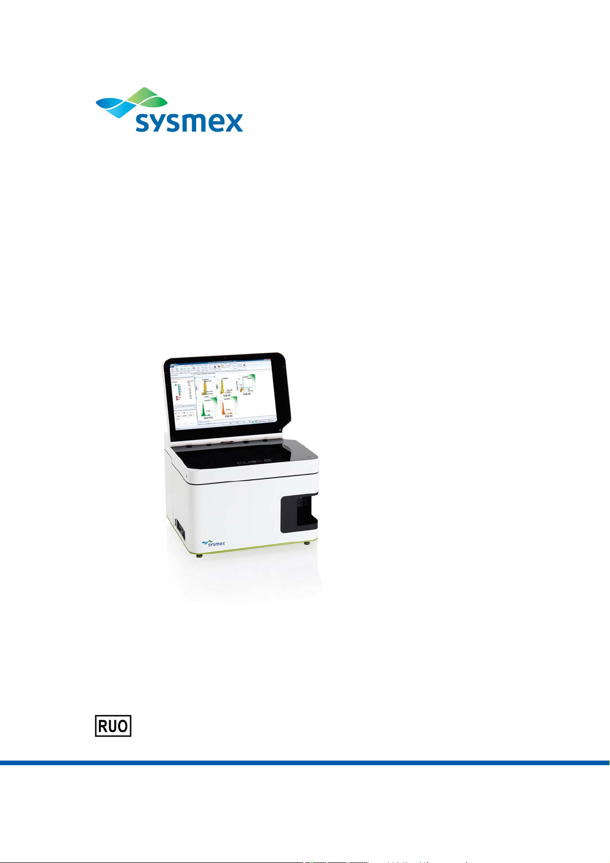
CyFlow® Cube 8
Operating Manual
For Research Use Only. Not for use in diagnostic procedures.
CyFlow® Software Version 1.0 RUO
Doc. No.: CY-S-3068RIFUEN | Doc. Rev
.: 032 | 17-05-2018 | EN | CN 383
Page 2

Imprint
Original Operating Manual
Sysmex Partec GmbH
Am Flugplatz 13
D-02828 Görlitz Germany
www.sysmex-partec.com
All rights reserved. No part of this manual may be reproduced, transcribed or translated in any form
or by any means electronic or otherwise, without the prior permission of Sysmex Partec GmbH.
2 CyFlow
®
Cube 8 | Operating Manual | May 2018 | Revision 032
Page 3

Table of contents
1 Introduction .............................................................................................6
1.1 About this operating manual .................................................... 6
1.2 Typographical conventions ...................................................... 7
1.3 General conditions ....................................................................8
1.4 CE compliance ........................................................................... 8
2 Safety ....................................................................................................... 9
2.1 Intended use...............................................................................9
2.2 Prohibited use ............................................................................9
Table of contents
2.3 Reasonably foreseeable misuse ..............................................9
2.4 User definition..........................................................................10
2.4.1 User qualification groups ...........................................................10
2.4.2 User qualification table...............................................................11
2.5 Environmental conditions.......................................................11
2.6 Prohibition and warning signs on the device ....................... 12
2.7 Personal protective equipment .............................................. 12
2.8 Laser safety .............................................................................. 13
2.9 Electrical safety........................................................................13
2.10 Alterations to the device ......................................................... 13
3 Overview ................................................................................................ 14
3.1 Components of the device ......................................................17
3.2 Type plate ................................................................................. 18
3.3 Scope of delivery ..................................................................... 19
3.4 Accessories and spare parts .................................................. 21
4 Transport and storage..........................................................................22
5 Installation .............................................................................................23
5.1 Positioning the device.............................................................23
5.2 Installation and uninstallation ................................................ 23
CyFlow® Cube 8 | Operating Manual | May 2018 | Revision 032 3
Page 4

Table of contents
6 Operation ...............................................................................................24
6.1 Inserting the Software dongle.................................................24
6.2 Start-up procedure...................................................................24
6.2.1 Switching on the device .............................................................24
6.2.2 Logging in and logging out.........................................................25
6.2.3 Performing a Prime ....................................................................26
6.3 Performing a measurement.....................................................27
6.4 Performing an intermediate cleaning.....................................28
6.5 Shutdown procedure ...............................................................29
6.5.1 Cleaning for shutdown ...............................................................29
6.5.2 Switching off the device .............................................................29
6.6 Software operation...................................................................30
6.6.1 Preparing measurements using the Worklist .............................30
6.6.2 Analysing data and creating reports using the Playlist...............37
7 Troubleshooting....................................................................................39
7.1 Performing a de-bubble procedure ........................................39
7.2 Performing a de-clog procedure.............................................39
7.3 Sheath fluid, waste and fluids.................................................40
7.4 Calibration and Count Check Beads (low, medium, high) ...41
7.5 Measurements and data acquisition ......................................41
8 Cleaning.................................................................................................42
8.1 Cleaning the device .................................................................42
8.2 Performing a cleaning procedure...........................................43
9 Maintenance ..........................................................................................44
10 Disposal .................................................................................................45
11 Technical data .......................................................................................46
4 CyFlow
®
Cube 8 | Operating Manual | May 2018 | Revision 032
Page 5

Table of contents
12 Software description ............................................................................50
12.1 Overview ...................................................................................50
12.2 Views of the software window ................................................ 52
12.3 Quick Access Toolbar ............................................................. 56
12.4 Ribbon.......................................................................................58
12.4.1 File tab .......................................................................................58
12.4.2 Home tab ...................................................................................65
12.4.3 Analyze tab ................................................................................ 68
12.4.4 Preview tab ................................................................................ 74
12.4.5 Parameters tab ..........................................................................76
12.4.6 Compensation tab......................................................................84
12.4.7 Statistics tab...............................................................................92
12.4.8 Worklist tab ................................................................................ 97
12.4.9 Playlist tab................................................................................100
12.4.10 Cytometer tab ..........................................................................105
12.4.11 Overlay tab...............................................................................109
12.4.12 Report tab ................................................................................114
12.4.13 Views tab .................................................................................123
12.4.14 Plot Format tab ........................................................................124
12.4.15 Region Format tab ...................................................................128
12.4.16 Overlay Format tab .................................................................. 131
12.5 Panes ......................................................................................136
12.5.1 FCS File Information pane....................................................... 137
12.5.2 Results Hierarchy pane............................................................138
12.5.3 Settings pane........................................................................... 139
12.5.4 Acquire pane............................................................................140
12.5.5 Setup pane...............................................................................143
12.5.6 Stops pane...............................................................................144
12.6 Worklist pane .........................................................................146
12.7 Playlist pane ........................................................................... 154
12.8 Workspace..............................................................................160
12.8.1 Plots tab of the Workspace...................................................... 160
12.8.2 Results tab of the Workspace.................................................. 171
12.8.3 Overlays tab of the Workspace................................................174
12.8.4 Reports tab of the Workspace .................................................179
12.9 Status bar ...............................................................................184
12.10 CyFlow Options......................................................................187
Index.....................................................................................................195
CyFlow® Cube 8 | Operating Manual | May 2018 | Revision 032 5
Page 6

1Introduction
1 Introduction
1.1 About this operating manual
This operating manual will help you to operate your CyFlow® Cube device.
Emphasis is placed on the installation, start-up and safe operation of the
device.
The basic principles of flow cytometry can be found in the medical literature
(e.g. Howard M. Shapiro, Practical Flow Cytometry, Wiley 2003).
This operating manual comes with the device. Read this operating manual
thoroughly before using the device. Please keep this operating manual for
future reference.
This operating manual is divided in two parts. The first part, chapter 1–11,
gives the user all necessary information for safe handling, scope of delivery,
to set up the device and how to operate the device properly. The general use
of the software and the typical workflows are described in chapter 6.5. This
chapter also is suitable to get to know the functioning of your device.
In the second part, chapter 12, you will find a description of all software
functions and a detailed description of the user interface. This chapter is for
reference.
There are product data sheets for the reagent kits and application notes
available. Please also refer to these documents.
If you have any questions about the content of this operating manual or the
use of the device, contact your local Sysmex representative.
6 CyFlow
®
Cube 8 | Operating Manual | May 2018 | Revision 032
Page 7
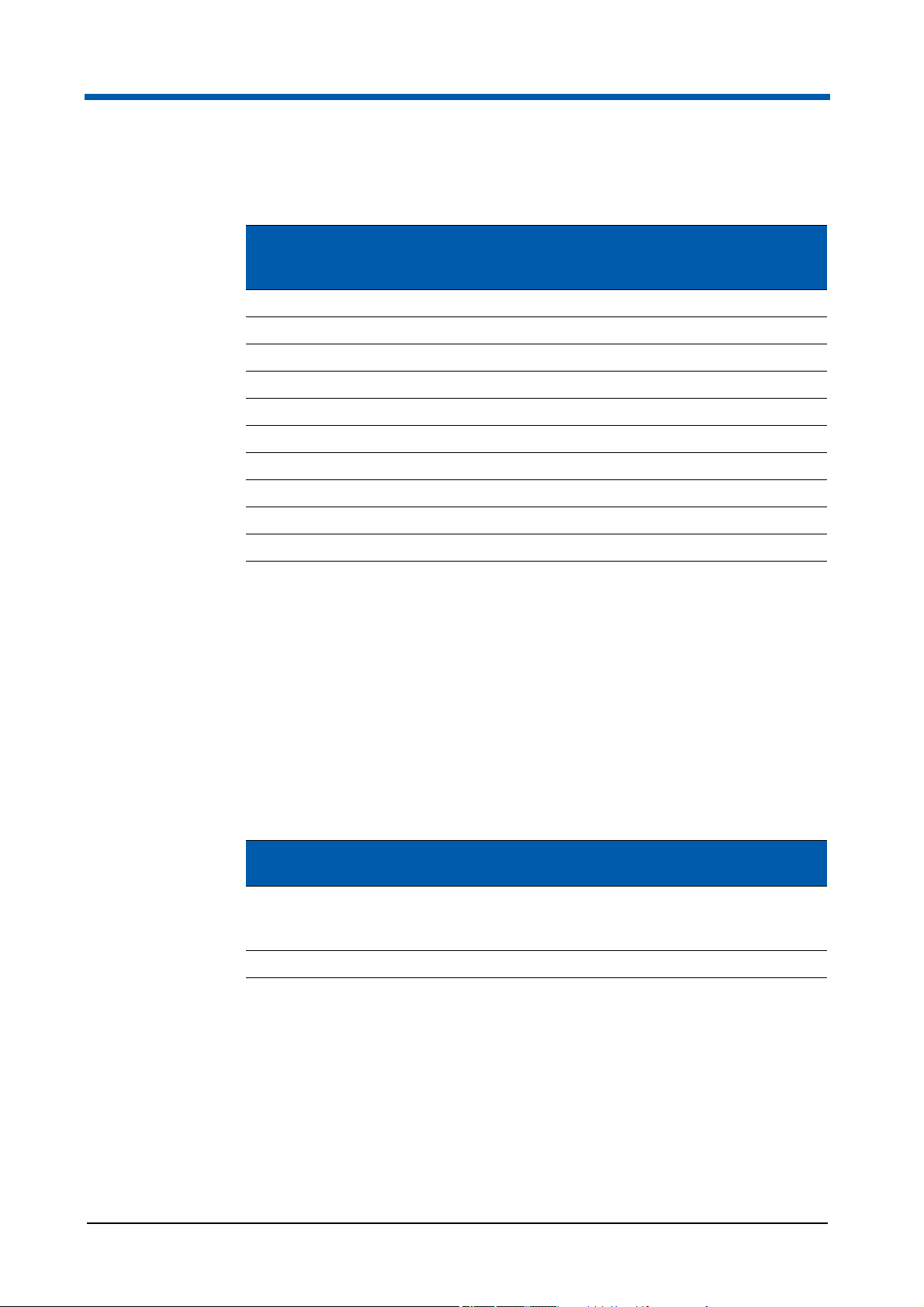
1.2 Typographical conventions
In this operating manual, warnings are indicated by a signal word. Hazards
are categorised into hazard levels with consequences of differing severity.
Type of hazard
This will result in death or have a serious impact on health.
Information about avoiding the hazard.
1Introduction
Type of hazard
This could result in death or have a serious impact on health.
Information about avoiding the hazard.
Type of hazard
This may have a minor impact on health.
Information about avoiding the hazard.
Type of hazard
This could result in material damage.
Information about avoiding the hazard.
All warnings are structured according to the same model. The type of hazard
is stated after the signal word. Then the consequences that may result from
the hazardous situation are described. And finally, how the hazardous
situation can be avoided.
CyFlow® Cube 8 | Operating Manual | May 2018 | Revision 032 7
Page 8

1Introduction
1.3 General conditions
Ensure that the following conditions are met when working with the device:
This operating manual must be read prior to using the device.
Report any recurring faults or problems to your local Sysmex
Sysmex Partec GmbH does not accept liability for any damage or personal
injury arising from:
Modifications or manipulation of the device;
Improper use;
Use of non-approved accessories;
Improper handling;
Non-compliance with this operating manual.
representative.
1.4 CE compliance
The device is marked with a CE mark of conformity, which confirms the
compliance with the essential requirements of the following European
Directives:
2014/35/EC on electrical equipment designed for use within certain
voltage limits;
2014/30/EC on electromagnetic compatibility;
2011/65/EC on the restriction of the use of certain hazardous substances
in electrical and electronic equipment.
1.5
8 CyFlow
®
Cube 8 | Operating Manual | May 2018 | Revision 032
Page 9

2 Safety
2.1 Intended use
2 Safety
For Research Use Only. Not for use in diagnostic procedures.
The device is a flow cytometer, it offers automation for routine use and
flexibility for research use in the field of flow cytometric applications.
The applications cover:
Multi-colour analysis of immune cells for research purposes;
Leukocyte counting/rare event analysis for research purposes;
Microbiological analysis;
Fermentation control;
Bead-based assays for research purposes;
Particle and cell concentration analysis based on True Volumetric
Absolute Counting;
Particle size and fluorescence distribution analysis.
2.2 Prohibited use
Never use the device with organic solvents as this can destroy the fluidic
system. Only use particles with a diameter < 100 µm. Only use Sysmex
approved fluids for sheath, cleaning and decontamination.
Never for use in diagnostic procedures.
2.3 Reasonably foreseeable misuse
Only use this device as a sensitive measuring device. It should:
NOT be used as personal computer.
NOT be used with chemicals harmful to the device (household sanitisers
etc.).
CyFlow® Cube 8 | Operating Manual | May 2018 | Revision 032 9
Page 10

2 Safety
2.4 User definition
The device may only be used by personnel properly instructed in its
handling. The manufacturer, authorised distributor or a person authorised by
the operator (and trained by either the manufacturer or an authorised
distributor) must provide instruction in handling the device with the help of
this operating manual.
The device is aimed for a large spectrum of users, from beginners to
experts. In the best case an expert is around – so, if you are a beginner, let
her/him help you.
Access to the device is not permitted to insufficiently qualified personnel.
2.4.1 User qualification groups
Instructed personnel
Instructed personnel have to be trained by qualified personnel or personnel
authorised by Sysmex to operate the device within the scope of the intended
use. They have to be able to assess if the device can be safely used and are
proficient in handling hazardous substances.
Qualified personnel
Qualified personnel have in-depth knowledge of the device and the
applications. They have been trained by personnel authorised by Sysmex to
operate the device, to perform cleaning and certain maintenance operations.
Qualified personnel have a scientific or technical education and several
years of experience in flow cytometry and are proficient in handling
hazardous substances.
Authorised service personnel
Personnel conducting technical service must be authorised by Sysmex.
Please contact the service department of your local Sysmex representative.
10 CyFlow
®
Cube 8 | Operating Manual | May 2018 | Revision 032
Page 11
2.4.2 User qualification table
2 Safety
Activity Instructed
personnel
Transport × ×
Installation ×
Operation × × ×
Cleaning × × ×
Decontamination × ×
Maintenance ×¹ ×¹ ×
Technical service ×
Uninstalling × ×
Packing × ×
Disposal × ×
× = activity can be performed by the user
¹ = please refer to the maintenance table for detailed instructions (see
chapter 9 Maintenance on page 44).
Qualified
personnel
Authorised
service
personnel
2.5 Environmental conditions
The device may only be used in laboratories. The specified ambient
temperature and relative humidity conditions must be maintained at all times.
The laboratory environment must be clean. Direct sun light should be
avoided.
CyFlow® Cube 8
Configuration
V1, V2, V4, V5, V6,
V7, V8, V9, V10,
V11
N1 15 °C to 30 °C
Relative humidity: between 20 % and 85 %, non-condensing.
Operating temperature range
15 °C to 30 °C
CyFlow® Cube 8 | Operating Manual | May 2018 | Revision 032 11
Page 12
2 Safety
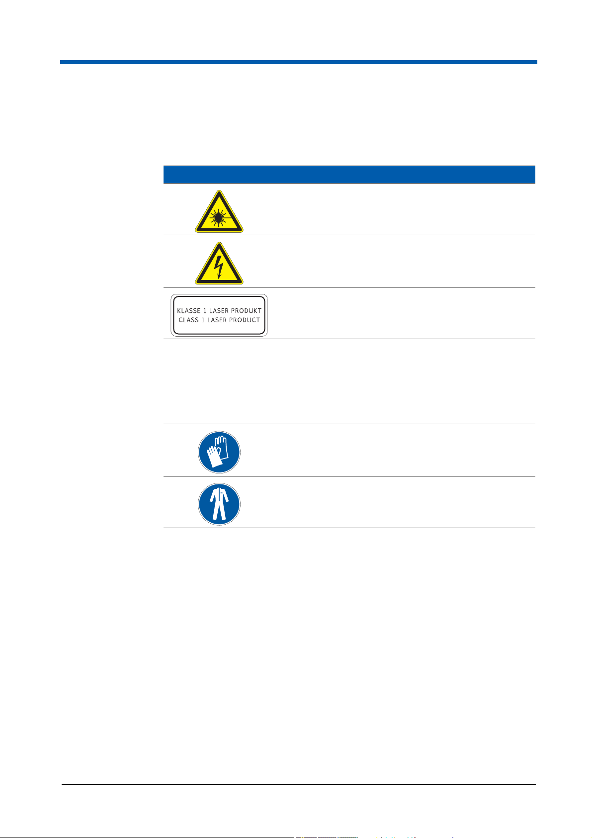
2.6 Prohibition and warning signs on the device
The following prohibition and warning signs have been affixed to the device.
Warning sticker Meaning
Laser radiation
Electrical hazards
Beware of electrical currents and electrical shocks
Additional laser labelling
2.7 Personal protective equipment
The following personal protective equipment is recommended to operate the
device.
Gloves must be worn at all times.
Lab coat must be worn at all times.
12 CyFlow
®
Cube 8 | Operating Manual | May 2018 | Revision 032
Page 13
2.8 Laser safety
The device is equipped with a class IIIb laser unit. If the housing of the
device is closed, the laser class of the laser unit is classified as a laser
class I (EN 60825-1:2015).
Never open the housing of the device.
Laser light of laser class IIIb can be emitted if the housing of the device is
damaged or the laser protection is removed. Serious injuries of the eyes and
the skin are the results of emission of laser light of laser class IIIb.
2.9 Electrical safety
The main electrical source used must be grounded or earthed due to local
specifications.
2 Safety
Please place the device in such a way that the electrical power cord can
easily be unplugged. Removable power cords should not be replaced by
inadequate wiring.
Beware of possible voltage when changing the fuse (T 4.0 A 250 V).
2.10 Alterations to the device
Unauthorised alterations to the device can result in risks and hazards.
Therefore, unless expressly permitted by the manufacturer, no alterations
may be made to the device.
If the device is altered, appropriate tests and trials must be performed to
ensure the continued safe use of the device.
2.11
CyFlow® Cube 8 | Operating Manual | May 2018 | Revision 032 13
Page 14
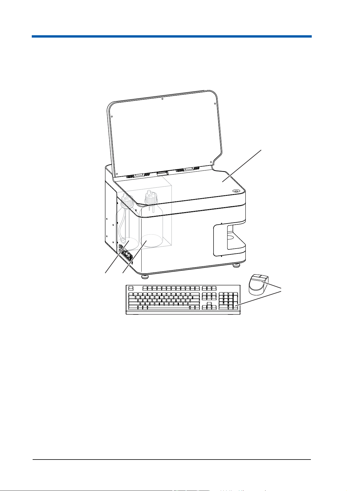
3Overview
5
1
2
3
4
3Overview
Your CyFlow® Cube device is a fully equipped desktop Flow Cytometer
(FCM). Which features a modular optical concept. This allows different
lasers with different wavelength ranges be used as light sources and the
detection of up to 8 optical channels (parameters).
The device allows the optics to be optimised for any application simply by
exchanging optical filters and mirrors. The device runs with an internal PC.
Data acquisition, device control, and data analysis are controlled and
performed by the software.
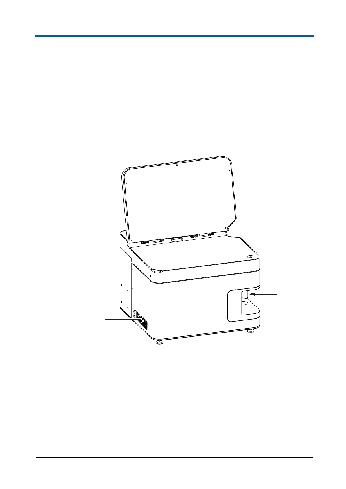
Fig. 3.1 Front and left side of the device
14 CyFlow
1 On switch
2 Sample port
3 Ports for external devices
®
Cube 8 | Operating Manual | May 2018 | Revision 032
4 Sliding compartment
5 Display
Page 15
3Overview
1 3
15
14
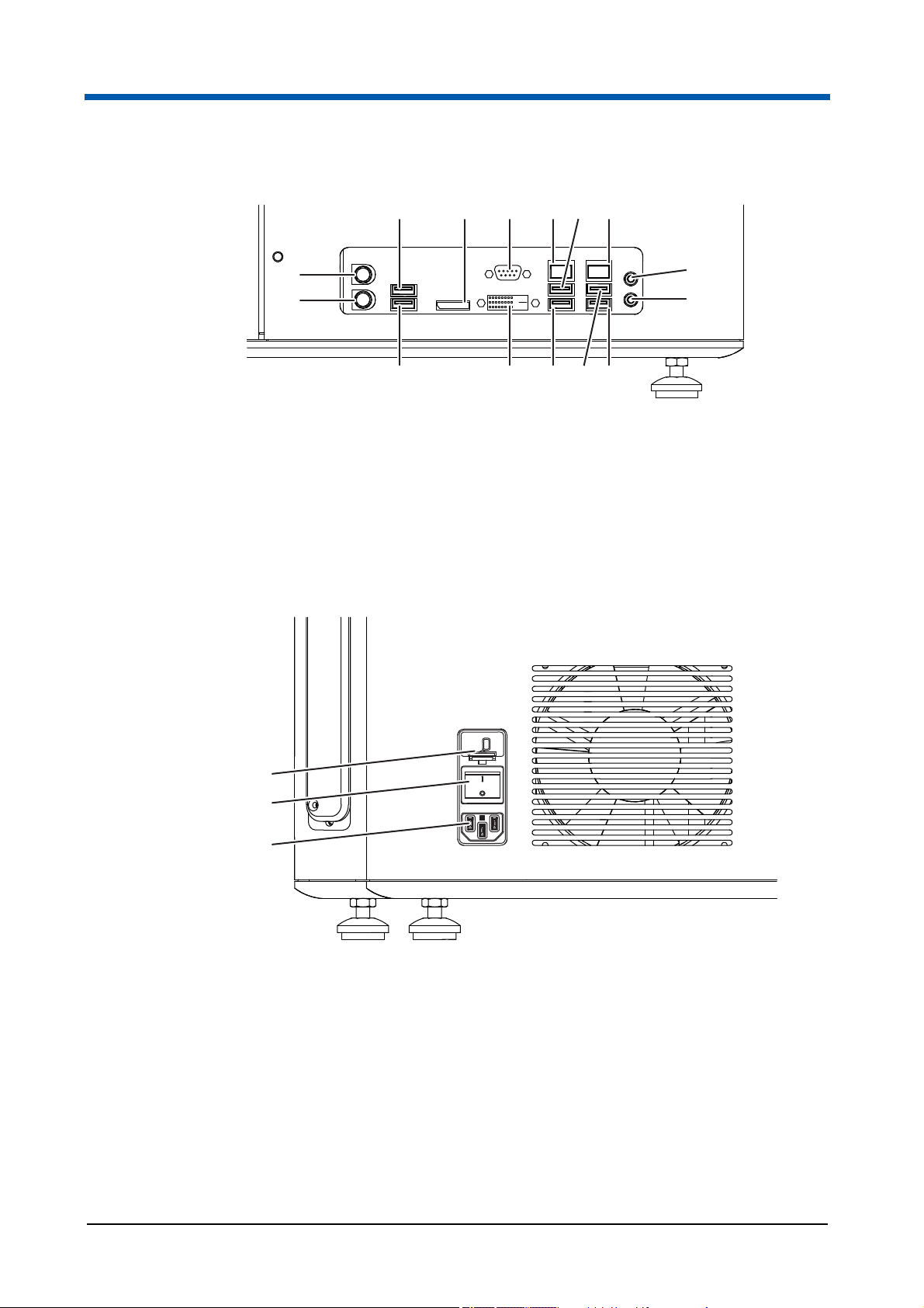
Fig. 3.2 Ports for external devices
1 USB port
2 HDMI port
3 VGA port
4 Ethernet port
5 USB port
6 Ethernet port
7 Audio port
8 Audio port
2 4 5 6
7
8
1213 91011
9 USB port
10 USB port
11 USB port
12 DVI port
13 USB port
14 Keyboard port
15 Mouse port
1
2
3
Fig. 3.3 Rear side of the device
1 Fuse insert (T 4.0 A 250 V)
2 Power switch
3 Connector socket for the power cord
CyFlow® Cube 8 | Operating Manual | May 2018 | Revision 032 15
Page 16
3Overview
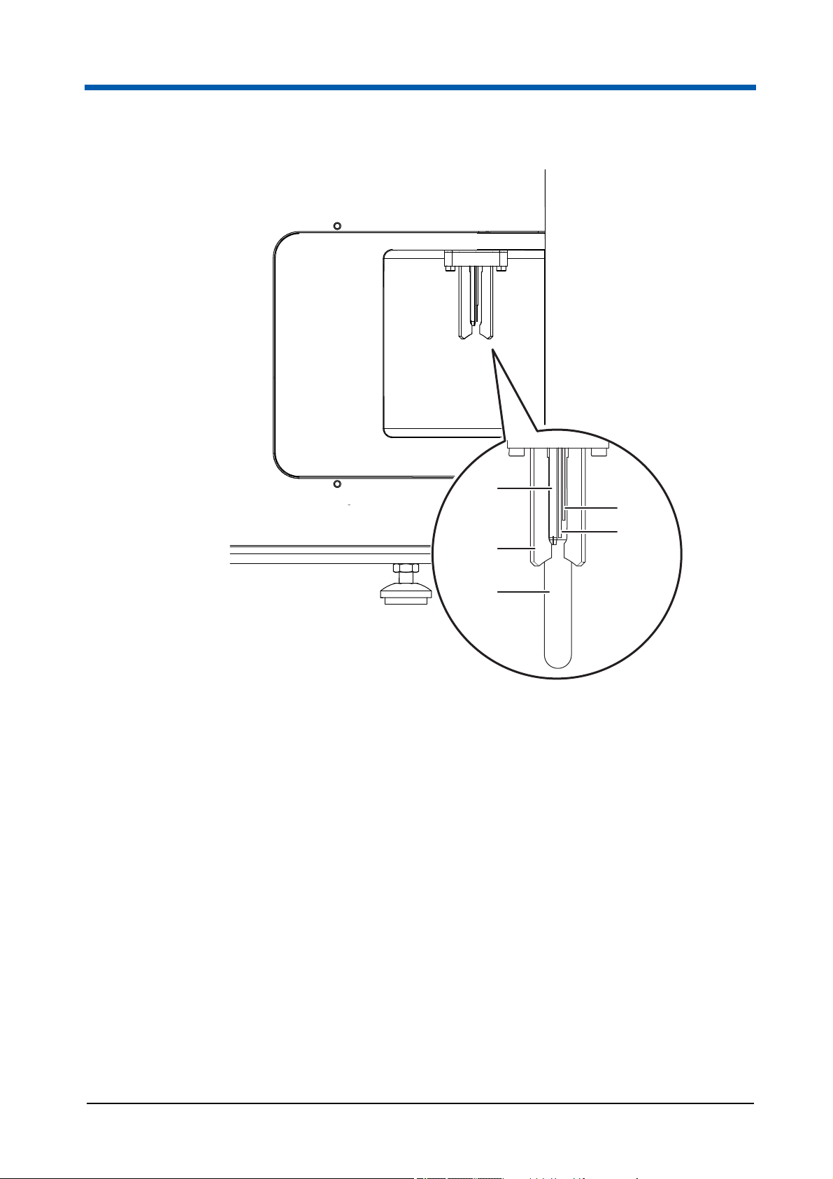
5
1
2
4
3
Fig. 3.4 Sample port at the right side of the device
1 Start electrode
2 Stop electrode
3 Sample tube
16 CyFlow
4 Sample holder
5 Sample port injection needle
®
Cube 8 | Operating Manual | May 2018 | Revision 032
Page 17

3.1 Components of the device
The device contains the flow cuvette, the optics, the fluidics, the computer
unit and data acquisition electronics. No work steps inside the device are
necessary.
The main components of the device are:
Control elements
The device is operated via keyboard and mouse. The On switch is located
on the top, when the display of the device is lifted up. The power switch is
located on the rear side of the device.
Computer interface ports
The computer interface ports connect the device with additional optional
electronic devices. They are located on the left side of the device.
3Overview
Sheath fluid bottle and waste bottle
The sheath fluid transports the sample flow during the measurement.
The connecting ports for the tubings of the sheath fluid bottle and waste
bottle are located inside the device. The tubings are preinstalled. The sheath
fluid bottle and waste bottle are located in the sliding compartment at the
rear side of the device.
Sample port with electrodes
The sample port is located on the right side of the device.
The sample port holds the sample tube during the measurement. The start
and stop electrodes of the sample port allow the independent determination
of exact 200 μL volume for each sample. The method of True Volumetric
Absolute Counting (TVAC) supported by CyFlow
the precise measurement of a fixed sample volume.
®
Cube systems is based on
CyFlow® Cube 8 | Operating Manual | May 2018 | Revision 032 17
Page 18
3Overview
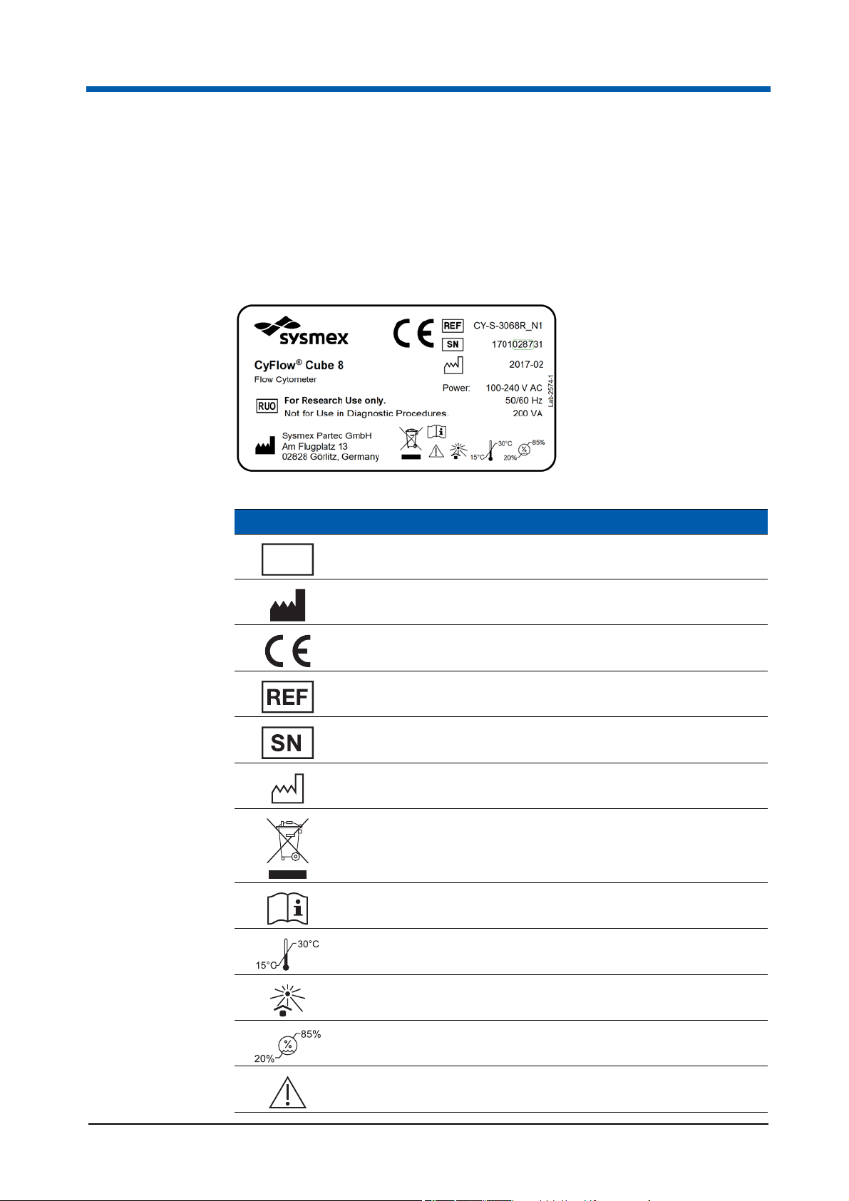
3.2 Type plate
The type plate is attached to the rear side of the device.
The content of the type plate varies according to the system configuration.
The system configuration is represented by an addition to the REF number
(e.g. CY-S-3068R_N1).
The following signs are part of the type plate which has been affixed to the device.
Symbol Meaning
RUO
For Research Use Only
Manufacturer
Certification mark
Reference Number
Serial Number
Manufacturing date
Waste of Electrical and Electronic Equipment
Operating manual
Indicates the temperature limits to which the device can be
safely exposed
No direct sunlight at the installation location
Indicates the range of relative humidity to which the device
can be safely exposed
Caution
18 CyFlow
®
Cube 8 | Operating Manual | May 2018 | Revision 032
Page 19
3.3 Scope of delivery
3Overview
1
4 3
Fig. 3.5 Scope of operation
1 CyFlow® Cube device
2 Keyboard and mouse
3 Waste bottle
4 Sheath fluid bottle with inline filter for
sheath fluid
The scope of delivery includes:
1 CyFlow
1 Power cord;
1 Software dongle;
1 Operating manual;
1 Laboratory bottle, 1 litre, labeled with sheath;
1 Laboratory bottle, 1 litre, labeled with waste;
®
Cube device;
2
CyFlow® Cube 8 | Operating Manual | May 2018 | Revision 032 19
Page 20

3Overview
1 Blue cap with electrodes, cabling and tubing for sheath including inline
filter;
1 Red cap with electrodes, cabling and tubing for waste.
The scope of operation includes:
1 CyFlow
1 Power cord;
1 Software dongle;
1 Operating manual;
1 Keyboard and 1 mouse;
1 Laboratory bottle, 1 liter, labeled with sheath;
1 Laboratory bottle, 1 liter, labeled with waste;
1 Blue cap with electrodes, cabling and tubing for sheath;
®
Cube device;
1 Red cap with electrodes, cabling and tubing for waste.
20 CyFlow
®
Cube 8 | Operating Manual | May 2018 | Revision 032
Page 21

3.4 Accessories and spare parts
Additional available application accessories and spare parts:
Product name Content Order No.
Sheath fluid 5000 ml 04-4007_R
Sheath fluid tap 1 piece 04-4006
Cleaning solution 250 ml 04-4009_R
3Overview
Decontamination
250 ml 04-4010_R
solution
Hypochlorite solution 250 ml 04-4012_R
Count Check Beads
50 tests 05-4010
(low, medium, high)
Calibration Beads 1 µm
1 ml 05-4007
Concentrate
Calibration Beads
30 ml 05-4018
3 µm, ready-to-use
DNA Control PI 25 ml 05-7303
DNA Control UV 25 ml 05-7302
Sheath fluid bottle 1l 1000 ml empty bottle 04-200-1041
Waste bottle 1l 1000 ml empty bottle 04-200-1042
Cap for 1 l glass
1 piece 04-200-1056
sheath fluid bottle
Cap for 1 l glass
1 piece 04-200-1057
waste bottle
Sample tube 3.5 ml 500 pieces 04-2000
Keyboard 1 piece 06-500-1040
Mouse 1 piece 06-500-1041
Spare fuses T 4,0 A 5 pieces 06-7-8006
Additional available upgrades:
CyFlow
CyFlow® Sorter for CyFlow
®
Robby 8 Autoloading Station
®
Cube
Visit our website http://www.sysmex-partec.com or contact your local
Sysmex representative for further information about our products.
3.5
CyFlow® Cube 8 | Operating Manual | May 2018 | Revision 032 21
Page 22

4 Transport and storage
4 Transport and storage
Warning! The weight of the device is about 40 kg.
Always have at least two people carry or lift the device.
In order to transport the device to a different location all external data and
supply connections have to be disconnected.
The device should be carried in an upright position.
The device is supplied in packaging that protects it against damage and
contamination. Please retain the packaging. Place the device in the
packaging for transport and storage.
The storage environment must be dry, clean and dust-free:
Storage temperature: between 5 °C and 50 °C;
Relative humidity: between 20 % and 85 %, non-condensing.
4.1
22 CyFlow
®
Cube 8 | Operating Manual | May 2018 | Revision 032
Page 23
5 Installation
5.1 Positioning the device
Heavy weight
When moving the device (packed or unpacked) or removing it from its
packaging, a person is exposed to a high risk of damaging his or her body
due to the heavy weight of the device.
At least two persons are required for transport and installation.
Carefully select the place where to position and operate the device. Comply
with the following criteria when positioning the device:
5 Installation
Place the device on a solid, dry and clean horizontal surface.
Avoid smoke, dust, vibrations, direct sunlight and any source of direct
heat.
Leave a minimum distance of 15 cm between the back of the device and
a wall to keep the ventilation effective.
Do not block the ventilation grid at the back of the device.
Do not place any objects on the device.
5.2 Installation and uninstallation
Installation, connection, disconnection and uninstallation may only be
performed by authorised service personnel and in conformity with the
applicable national rules and regulations.
5.3
CyFlow® Cube 8 | Operating Manual | May 2018 | Revision 032 23
Page 24
6 Operation
6Operation
Due to heavy use of software-related content in the following chapter please
also refer to chapter 12 Software description on page 50.
6.1 Inserting the Software dongle
Procedure
1. Insert the included Software dongle into an open USB port of the device.
Result
The software will check automatically in regular intervals if the dongle is
plugged in. If the dongle is not plugged in, the software will not be
functional.
6.2 Start-up procedure
Old sheath fluid
Old sheath fluid affects the sample flow through the flow cuvette.
Replace the sheath fluid at least once a week or before any daily use.
6.2.1 Switching on the device
Before switching on the device make sure the sheath fluid bottle is filled with
800 ml of clean, filtered and degassed sheath fluid and is closed with the
blue screw cap. It is recommended to replace the sheath fluid at least once a
week or before any daily use.
Requirements
The sheath fluid bottle is filled and connected to the device.
The waste bottle is empty and connected to the device.
Procedure
1. Switch on the device using the power switch on the rear side of the device.
2. Lift up the display of the device.
3. Push the On switch on the top of the device.
– The device is switched on.
24 CyFlow
®
Cube 8 | Operating Manual | May 2018 | Revision 032
Page 25
4. Start the software by double click the CyFlow® Software icon.
– The log-in dialogue is displayed.
– The device is, by default, set in a standard mode.
6.2.2 Logging in and logging out
Each user is assigned to a user role. Each user role has specific privileges.
Some functions of the software are not available for each user role and
availability depends on the assigned privileges.
User management
Role Privileges
Service operator User administration
6Operation
Worklist creation
Logging in
Worklist management
Sample analysis
Manage Workspace and settings
Create comp setup
User administrator User administration
Parameter properties
Assay developer Manage Workspace and settings
Worklist creation
Worklist management
Sample analysis
Create comp setup
Requirements
The log-in dialogue is displayed.
User access must be set up and the user name and password must be
known to log into the software.
Procedure
1. Enter the user name.
2. Enter the password.
3. Click the Log-in button.
– The log-in dialogue closes.
– The user role dialogue will be displayed.
CyFlow® Cube 8 | Operating Manual | May 2018 | Revision 032 25
Page 26

6 Operation
Logging out
4. Select the respective user role.
5. Click the OK button.
– If the log-in was successful the start screen is displayed.
After a specified number of unsuccessful login attempts (default 3), the
account will be locked. If the account is locked, please contact a user with
the "user administration" privilege in its user role, e. g. a user administrator.
The default settings for logins can be changed in the user management.
Procedure
1. On the File tab of the Ribbon (see chapter 12.4.1 File tab on page 58)
click the Log-out button.
– The current user is logged out.
– The log-in dialogue is displayed.
6.2.3 Performing a Prime
A Prime mode is available as a start-up process for the device. This process
includes cleaning, filling the tubes with sheath fluid and controlling the device
set-up.
The Prime should be performed in the following cases:
Starting the device for the first time of the day,
After the sheath fluid bottle has been filled,
As a trouble-shooting procedure (no/bad signals, blocking, etc.).
Requirements
Sample tube with 1.6 ml Decontamination Solution (Order No.
04-4010_R) connected.
Procedure
1. On the Cytometer tab of the Ribbon (see chapter 12.4.10 Cytometer tab
on page 105) or on the Acquire pane (see chapter 12.5.4 Acquire pane
on page 140) click the Prime button.
– The instruction dialogue for the Prime procedure is displayed.
2. Follow the instructions until the finish message is displayed.
– The device is ready for the sample measurements.
3. Remove emptied sample tube.
26 CyFlow
®
Cube 8 | Operating Manual | May 2018 | Revision 032
Page 27

6.3 Performing a measurement
Requirements
The device is primed.
The respective Worklist is loaded.
A Worklist item is active with a defined Workspace.
The Worklist contains at least one defined item that does not contain a
listmode file.
The sample is prepared for the measurement.
The sheath fluid is not low.
The waste level is not high.
Procedure
6Operation
1. Fill the sample tube with the sample fluid.
2. Insert the sample tube into the sample port of the device until the sample tube audibly clicks.
3. On the Acquire pane (see chapter 12.5.4 Acquire pane on page 140)
click the Start button.
– Data acquisition starts. Progress is displayed in the status bar.
4. If a stop condition is set, wait until acquisition stops.
If no stop condition is set, click the Stop button on the Acquire pane to
stop acquisition.
– A measurement is performed.
5. Remove emptied sample tube.
CyFlow® Cube 8 | Operating Manual | May 2018 | Revision 032 27
Page 28

6 Operation
6.4 Performing an intermediate cleaning
A cleaning mode is available to clean the device when a different sample
type is to be measured.
Requirements
Log-in as a user with the respective role.
The respective Worklist is loaded.
Sample tube with 1.6 ml Cleaning Solution (Order No. 04-4009_R)
connected.
Procedure
1. On the Cytometer tab of the Ribbon (see chapter 12.4.10 Cytometer tab
on page 105) click the Clean button.
– An instruction dialogue is displayed.
2. Follow the instructions until the finish message is displayed.
– An intermediate cleaning was performed.
– The device is ready for the next sample measurement.
28 CyFlow
®
Cube 8 | Operating Manual | May 2018 | Revision 032
Page 29

6.5 Shutdown procedure
6.5.1 Cleaning for shutdown
Perform the shutdown cleaning procedure to close the software.
Requirements
No acquisition is in progress.
Sample tube with 1.6 ml Decontamination Solution (Order No.
04-4010_R) connected.
Procedure
1. On the File tab of the Ribbon (see chapter 12.4.1 File tab on page 58)
click the Exit CyFlow Software button.
– If the Worklist or Playlist is currently open and has been modified, a
save changes dialogue appears.
6Operation
– A dialogue asking for a shutdown cleaning procedure appears.
2. Select Yes in the dialogue.
– The dialogue closes and initiates the shutdown cleaning procedure.
– After the cleaning procedure is complete the software closes.
3. Remove emptied sample tube.
6.5.2 Switching off the device
Requirements
The shutdown cleaning procedure was successful and the software is
closed.
Procedure
1. In the Windows menu, click the Shut down button.
– The device shuts down.
2. Switch off the device using the power switch on the rear side of the device.
– The device is switched off.
CyFlow® Cube 8 | Operating Manual | May 2018 | Revision 032 29
Page 30

6 Operation
6.6 Software operation
The software can be run in two different modes:
In Worklist mode, data can be acquired. The hardware and software
settings for each measurement are predefined and organised in a list
called Worklist.
In Playlist mode, acquired data can be analysed and settings for future
measurements can be prepared. Files are organised and edited in a
Playlist.
This chapter describes how to use a Worklist for preparing sample
measurements and how to use a Playlist to analyse data. For a detailed
description of software functions, see chapter 12 Software description on
page 50.
6.6.1 Preparing measurements using the Worklist
This chapter describes the typical sequence of steps when preparing a
Worklist for future measurements.
A Worklist contains the predefinitions of hardware and software settings for
data acquisition (see chapter 12.6 Worklist pane on page 146). These
predefinitions are set prior to measurements when preparing the Worklist.
Preparing the Worklist includes:
Defining the Workspace that contains the plots, regions and gates to
represent the cell populations of interest;
Defining and adapting the instrument settings to reduce background and
to position the populations of interest properly into the plots;
Performing a manual compensation to compensate for fluorescence
spillover as appropriate.
These settings can be preset prior to acquiring data and adapted while
measuring samples.
30 CyFlow
®
Cube 8 | Operating Manual | May 2018 | Revision 032
Page 31

Creating a new Worklist
Requirements
To create a Worklist for future measurements, login as an assay
developer is necessary.
Procedure
1. On the File tab of the Ribbon (see chapter 12.4.1 File tab on page 58)
select "File > New > New Worklist".
In Worklist mode, a new Worklist can also be created by clicking the New
button in the Worklist pane (see chapter 12.6 Worklist pane on
page 146).
– A new default Worklist containing 400 blank Worklist items is created
and displayed in the Worklist pane.
– The software is in Worklist mode.
6Operation
Defining a new Workspace
A Workspace contains the plots, regions and gates of interest (see chapter
12.8 Workspace on page 160). To prepare a new measurement, a
Workspace can be prepared before acquiring data and further adapted while
measuring a sample.
Procedure
1. Double-click a Worklist item to open it in the Workspace.
2. In the Worklist, enter a Lab # and sample ID for the Worklist item as desired.
3. Define which plots to be displayed in the Plots area of the Workspace:
On the Home tab of the Ribbon (see chapter 12.4.2 Home tab on
page 65), click the Density Plot button or the Histogram Plot button to
add a corresponding plot to the Workspace.
Alternatively, select the desired plots by double-clicking on the plots in
the Previews area of the Workspace.
4. To change the parameter for an axis of a plot, right-click on the axis and select the parameter from the drop-down list.
Alternatively, select the parameter from the Parameters group of the
Home tab of the Ribbon (see chapter Parameters group on page 66).
5. To change the scaling of the axes, select a plot, then select the scaling
(linear or logarithmic) on the Parameters group of the Home tab.
6. To change the plot title, double-click the current plot title and enter a new title.
– A new Workspace is defined.
CyFlow® Cube 8 | Operating Manual | May 2018 | Revision 032 31
Page 32

6 Operation
Presetting instrument settings
Procedure
1. Select the Settings pane (see chapter 12.5.3 Settings pane on
page 139).
2. To select a parameter as trigger parameter, set a parameter to "ON" in the "Logic" column (only available if all other parameters are set to "OFF").
Data of this parameter are acquired.
If desired, combine other parameters for trigger by setting them to "AND"
or "OR".
3. To predefine threshold values, enter a value in the "Threshold" column for the relevant parameters.
4. To predefine the signal intensity to be displayed for each parameter, enter a value in the "Voltage" column for the relevant parameters.
5. Select the Acquire pane (see chapter 12.5.4 Acquire pane on page 140).
6. Select the flow rate for the measurement by clicking the Low, Medium or High button or by using the flow rate slider.
– The selected flow rate is displayed next to the flow rate slider.
– The instrument settings are preset.
Starting measurement of the sample
Requirements
The device is primed.
A Worklist item is active with a defined Workspace.
Procedure
1. Insert the sample tube containing the sample into the sample port of the device until the sample tube audibly clicks.
2. On the Acquire pane (see chapter 12.5.4 Acquire pane on page 140)
click the Start button.
To refresh the view, click the Restart button on the Acquire pane.
– Data acquisition starts. Progress is displayed in the status bar.
– In the Plots tab of the Workspace (see chapter 12.8.1 Plots tab of the
Workspace on page 160) the plots display the acquired data.
32 CyFlow
®
Cube 8 | Operating Manual | May 2018 | Revision 032
Page 33

Adapting instrument settings during data acquisition
Procedure
1. Select the Settings pane (see chapter 12.5.3 Settings pane on
page 139).
2. In the "Voltage" column, adapt the voltage until the desired cell populations are displayed in the proper range in the plots and can be clearly separated.
When measuring an unstained control, edit the values for all
fluorescence parameters until the auto-fluorescence signals display
within the first/between the first and second decade of log scale.
3. In the "Threshold" column, adapt the threshold values to reduce background for each parameter triggered. Increase or decrease the threshold settings if the background is still too high or if the cell population of interest is cut off.
6Operation
Creating a region
To select the events of interest, regions can be created on the plots.
Procedure
1. Select the Home tab of the Ribbon (see chapter 12.4.2 Home tab on
2. To preselect creating an elliptical region, a rectangular region, a
3. For elliptical, rectangular or linear regions (on single-parameter plots),
– The instrument settings are adapted.
– The plots will automatically refresh according to the new instrument
settings.
page 65).
polygonal region, a linear region or a quadrant region, click the
corresponding button on the Region group (see chapter 12.4.2 Home tab
on page 65).
– The button is highlighted in orange.
draw out the region on the plot.
For a polygonal region, click on a plot to determine the first point of the
region, then click to define additional points. Complete the polygon by
clicking on the start point or by right-clicking.
For a quadrant region, click on the plot at the point you wish the
quadrant’s intercept point to appear.
4. To assign a name to the region, select the region and double-click the region name on the plot. Enter a region name in the edit field or select a name from the drop-down list.
Alternatively, select the region, select the Region Format tab of the
Ribbon (see chapter 12.4.15 Region Format tab on page 128) and use
CyFlow® Cube 8 | Operating Manual | May 2018 | Revision 032 33
Page 34

6 Operation
Setting a parent gate
the "Region Name" box to enter a name or to select a name from the
drop-down list.
– A region is created.
A region that contains all events of interest can be applied as a parent gate
to the other plots so that only the relevant events are displayed on these
plots. This gating will allow to focus on a subpopulation of cells only.
Procedure
1. In the Plots area of the Workspace, select the desired plot.
To select several plots, hold the Ctrl key while selecting or draw a
selection rectangle.
2. On the Home tab of the Ribbon (see chapter 12.4.2 Home tab on
page 65) click the arrow on the "Gate" box to expand a drop-down list
and select the desired region to be applied as a parent gate.
– A parent gate will be automatically created for the selected region.
– The parent gate will be applied to the selected plots, indicated by a
gate-coloured frame around the plots.
Stopping the measurement
If all described settings on the sample are set up, the measurement can be
stopped. When the sample is empty (the stop electrode is reached) or if a
stop condition is defined, measurement will stop automatically.
Procedure
1. On the Acquire pane (see chapter 12.5.4 Acquire pane on page 140)
click the Stop button.
– The measurement is stopped.
After finishing a measurement a dialogue box will appear. Press OK button
to proceed with an intermediate cleaning step. Please note that the
remaining sample will be aspirated during the cleaning step. Alternatively,
remove sample tube and press OK button. The cleaning step will be
performed with air. To skip the intermediate cleaning step press Cancel
button. The device is ready for the next sample measurement.
34 CyFlow
®
Cube 8 | Operating Manual | May 2018 | Revision 032
Page 35

Performing a manual compensation
A manual compensation can be performed online (during the measurement)
or offline (after data acquisition).
Procedure
1. On the Compensation tab of the Ribbon (see chapter 12.4.6
Compensation tab on page 84) click the Manual Compensation button
and the Plot Compensation button.
2. On the plot, draw the desired population of events into the required area of the plot.
If using a quadrant, statistics are displayed on the Compensation tab of
the Ribbon and can be used to arrange the population. Negative events
are displayed in the lower left quadrant. A population negative for a
parameter on Y scale should be placed in the lower right quadrant to the
same height as the negative events. A population negative for a
parameter on X scale should be placed in the upper left quadrant to the
same range as the negative events.
6Operation
For fine adjustment of compensation, use the arrow buttons on the
Compensation tab of the Ribbon. The direction of the arrow icons
indicates the way the plot populations move rather than the way the
compensation values change.
– A manual compensation is performed.
Saving the Workspace and the instrument settings
On completion of a sample measurement, an FCS file is automatically saved
containing the acquired data, the Workspace, the instrument settings and the
compensation. Workspace and instrument settings can additionally be saved
in separate files to use them independently.
Procedure
1. To save the Workspace of a Worklist item, select the File tab of the
Ribbon (see chapter 12.4.1 File tab on page 58) and select "File > Save
> Save Workspace" or "File > Save > Save Workspace As".
Alternatively, right-click the Worklist item in the Worklist to open the
context menu and select "Workspace > Save Workspace (As)".
– The Workspace is saved.
2. To save the instrument settings of a Worklist item, right-click the Worklist item in the Worklist to open the context menu and select "Instrument Settings > Save Instrument Settings".
– The instrument settings are saved.
CyFlow® Cube 8 | Operating Manual | May 2018 | Revision 032 35
Page 36

6 Operation
Defining the Worklist for remaining samples
Defining a Worklist for future measurements includes defining the
Workspace, instrument settings and stop conditions. Instrument settings and
stop conditions are loaded from the Workspace by default but can be
changed in the Worklist.
Procedure
1. In the Worklist, enter a Lab # and sample IDs for the Worklist items as desired.
2. To apply the Workspace developed from the sample to all Worklist items, right-click the Worklist item to open the context menu and select "Workspace > Apply To".
– A dialogue appears.
3. Select whether to apply the Workspace to the current panel or to the entire Worklist.
4. If differing instrument settings are to be used, click into the "Instrument Settings" cell of the Worklist item, select "Load from file" and select the desired instrument settings file.
5. To apply the differing instrument settings to other Worklist items, right-click the "Instrument Settings" cell to open the context menu and select "Apply to Panel".
6. To define differing stop conditions for the remaining samples, select the
desired stop conditions from the Stops pane (see chapter 12.5.6 Stops
pane on page 144).
Or right-click the "Stop Conditions" and "Stop Value" columns in the
Worklist to open the context menu and select the desired stop conditions.
– The Worklist for remaining samples is defined.
Saving the Worklist
The FCS data are saved automatically on completion of sample
measurement. The Worklist can be saved separately.
Procedure
1. To save the Worklist, select the File tab of the Ribbon (see chapter
12.4.1 File tab on page 58) and select "File > Save > Save Worklist" or
"Save Worklist As".
– The Worklist is saved.
36 CyFlow
®
Cube 8 | Operating Manual | May 2018 | Revision 032
Page 37

6.6.2 Analysing data and creating reports using the Playlist
Data can be analysed offline by using a Playlist (see chapter 12.7 Playlist
pane on page 154).
All data created for analyses, including plots, statistics, compensation
matrices and overlays, can be summarised in a page-based report that can
be printed.
Analysing data using the Playlist
Procedure
1. To create a new Playlist, select the File tab of the Ribbon (see chapter
12.4.1 File tab on page 58) and select "File > New > New Playlist".
In Worklist mode, a new Playlist can also be created by clicking the New
button in the Worklist pane (see chapter 12.6 Worklist pane on
page 146).
6Operation
Alternatively, drag and drop a Playlist file from the Windows Explorer into
the Workspace or the Playlist pane.
– A new blank Playlist is opened and displayed in the Playlist pane (see
chapter 12.7 Playlist pane on page 154).
– The software is in Playlist mode.
2. To open a Playlist item in the Playlist, select the File tab of the Ribbon
and select "File > Open > Open Listmode".
Alternatively, click the Open Listmode button on the Quick Access
Toolbar, or click the Open Listmode button on the Home tab of the
Ribbon (see chapter 12.4.2 Home tab on page 65), or drag and drop an
FCS file from the Windows Explorer into the Playlist, or press Ctrl + O.
3. Plots, regions and gates can be edited in the Plots tab of the Workspace as desired (see chapter 12.8.1 Plots tab of the Workspace on page 160).
4. Statistics can be displayed and edited in the Results tab of the
Workspace (see chapter 12.8.2 Results tab of the Workspace on
page 171).
5. In Playlist mode, for setting compensations, the Compensation Wizard
from the Compensation tab of the Ribbon can be used (see chapter
12.4.6 Compensation tab on page 84).
6. To save the compensation, select the File tab of the Ribbon and select
"File > Save > Save Compensation As".
7. For comparing plots to each other, overlay plots can be created manually
(see chapter 12.8.3 Overlays tab of the Workspace on page 174).
In Playlist mode, the Overlay Wizard on the Overlay tab of the Ribbon
can be used (see chapter 12.4.11 Overlay tab on page 109).
– The data are analysed.
CyFlow® Cube 8 | Operating Manual | May 2018 | Revision 032 37
Page 38

6 Operation
Creating a report
A report can be created manually in the Reports tab of the Workspace (see
chapter 12.8.4 Reports tab of the Workspace on page 179). Alternatively, in
Playlist mode, the Report Wizard from the Report tab of the Ribbon can be
used (see chapter 12.4.12 Report tab on page 114). When using the Report
Wizard, first select the page orientation, page size and header and footer
information (steps 1 to 4 in the following procedure).
Procedure
1. Select the Reports tab of the Workspace.
– A blank report page is displayed.
– The Ribbon switches to its Report tab.
2. From the Page Setup group on the Report tab of the Ribbon (see chapter
Pages group on page 119), select the desired page orientation (portrait
or landscape) and page size (A4 or letter).
3. From the Insert group on the Report tab of the Ribbon (see chapter Insert group on page 120select the items to be shown in the report.
4. Click on the desired section of the report page (header, body, footer) to insert the selected item in a default size or draw an insertion rectangle to get a custom size.
If using the Report Wizard, select the items to be shown in the header
and footer sections of all pages of the report here before starting the
Wizard.
5. Use the options provided in the Report tab of the Ribbon to insert and
organise pages, to edit text and other items and to arrange items.
– A report is created.
6.7
38 CyFlow
®
Cube 8 | Operating Manual | May 2018 | Revision 032
Page 39

7 Troubleshooting
If no data are displayed in the plots or histograms after acquisition process,
air bubbles or contaminations may have blocked the flow cuvette.
To solve this problem perform a de-bubble or de-clog procedure.
7.1 Performing a de-bubble procedure
Requirements
Log-in as a user with the respective role.
Procedure
1. On the Cytometer tab of the Ribbon, click the De-bubble button.
– An instruction dialogue is displayed.
7 Troubleshooting
2. Follow the instructions until the finish message is displayed.
– After successful de-bubble process the device is ready for the sample
measurements.
– If the de-bubble process was not successful, please contact your local
Sysmex representative.
7.2 Performing a de-clog procedure
Requirements
Log-in as a user with the respective role.
Procedure
1. On the Cytometer tab of the Ribbon, click the De-clog button.
– An instruction dialogue is displayed.
2. Follow the instructions until the finish message is displayed.
– After a successful de-clog process the device is ready for the sample
measurements.
– If the de-clog process was not successful, please contact your local
Sysmex representative.
CyFlow® Cube 8 | Operating Manual | May 2018 | Revision 032 39
Page 40

7 Troubleshooting
7.3 Sheath fluid, waste and fluids
Observation Possible solution
Sample flow is very
slow or is not
running.
Sample flow is very
fast even with low
speed.
Check that the waste bottle is closed properly and
that the bottle is not cracked.
Check all visible tubes and make sure that they are
not pinched.
Make sure that no air bubbles are trapped in the
yellow inline filter of the sheath fluid bottle.
Check the connection of the sample tube to the
sample port. Decant sample to another tube and
measure again.
Perform a priming procedure.
Perform a cleaning procedure.
Shut down the device, including the main switch on
the back side of the device. Wait 3–5 minutes and
re-start the system.
Check the speed settings.
Change the yellow inline filter (50 µm) of the sheath
fluid bottle.
Check if the visible sheath tube is pinched or
blocked.
Shut down the device, including the main switch on
the back side of the device. Wait 3–5 minutes and
re-start the system.
Check the speed settings.
40 CyFlow
®
Cube 8 | Operating Manual | May 2018 | Revision 032
Page 41

7 Troubleshooting
7.4 Calibration and Count Check Beads (low, medium, high)
Observation Possible solution
The results of the
Count Check Beads
(low, medium, high)
measurements are
not within ± 10%
range of the
lot-specific
concentration stated
Shake the bottle vigorously (e.g. by vortexing) and
repeat the measurement.
Check the date of expiry of the Count Check Beads
(low, medium, high).
Perform a priming procedure.
Perform a cleaning procedure.
on the bottle.
The results of the
Calibration Beads
measurements are
not in the
preselected regions
of the original
configuration script.
Check in software if you have loaded the correct
configurations for your measurement.
Shake the bottle vigorously (e.g. by vortexing) and
repeat the measurement.
Check the date of expiry of the Calibration Beads.
Perform a priming procedure.
Perform a cleaning procedure.
7.5 Measurements and data acquisition
Observation Possible solution
The device emits an
unusual / noisy
sound after starting
the measurement.
Check that the waste bottle is closed properly and
that the bottle is not cracked.
Check all visible tubes and make sure that they are
not pinched.
Check that liquid (sheath fluid and sample) is
dropping into the waste bottle after starting the
measurement.
Clean the two electrodes of the sample port
carefully by wiping them with a soft tissue soaked in
decontamination solution.
Perform a de-clog procedure.
There is no data
acquisition visible
(peaks/dots in
histogram/dot plot)
during the RUN
phase
Check in software if the laser/s is/are switched on.
Check if the right trigger parameter has been
selected (choose FSC trigger as default setting,
select SSC for very small cells, e.g. bacteria).
Check gain values and the threshold.
Increase the flow rate.
Perform a de-clog procedure.
7.6
CyFlow® Cube 8 | Operating Manual | May 2018 | Revision 032 41
Page 42

8 Cleaning
8 Cleaning
Contaminated sheath fluid bottle
A contaminated sheath fluid bottle disturbs the proper operation.
Clean the sheath fluid bottle regularly.
Using incorrect cleaning solvents
Using incorrect cleaning solvents when cleaning the casing and screen could
damage the device.
Do not use any organic solvents, nitro thinner, benzol, alcohol or highly
concentrated bleach.
Only use special screen cleaner.
8.1 Cleaning the device
The following list gives an overview of the various essential cleaning work on
the device.
Clean the device casing with a soft cloth on a regular basis carefully.
Water should not enter the device or peripheral devices or come into
contact with electric connections and switches.
Clean the screen with a soft cloth. Always use special screen cleaner.
Clean the sheath fluid bottle with distilled water and a brush. Flush with
clean distilled water several times.
Empty the waste bottle after and before each user session. When using
biohazardous samples, a volume of 50 ml of Hypochlorite Solution
(Order No. 04-4012_R) should be introduced into the waste bottle after
measurement or before emptying the waste.
If the device will not be used for longer periods, clean the flow system with
distilled water. Put a sample tube half-way filled with distilled water in the
sample port. Clean the waste bottle and the sheath fluid bottle, wipe top dry.
42 CyFlow
®
Cube 8 | Operating Manual | May 2018 | Revision 032
Page 43

8.2 Performing a cleaning procedure
The device can be cleaned between sets of samples using a Cleaning
Solution (Order No 04-4009_R) followed by a sample tube with sheath fluid.
This procedure will allow you to significantly reduce cross contamination and
reduce the background. There are three different levels of intensity available
that can be set: Default, quick or deep.
Requirements
Log-in as a user with the respective role.
Procedure
1. On the Cytometer tab of the Ribbon, click the Clean button.
– An instruction dialogue is displayed.
2. Follow the instructions until the finish message is displayed.
8Cleaning
– The device is ready for the sample measurements.
8.3
CyFlow® Cube 8 | Operating Manual | May 2018 | Revision 032 43
Page 44

9 Maintenance
9 Maintenance
Servicing is to be performed by an authorised service engineer. Please
contact your local Sysmex representative for further instructions.
Sequence Activity Minimum
user qualification level
Daily
maintenance
Weekly
maintenance
Quarterly
maintenance
Preventive
maintenance
Prime the device by using the Prime
function (see chapter 6.2.3 Performing a
Prime on page 26).
Priming should be performed:
– After starting the device;
– After the sheath fluid was changed;
– After the waste bottle was emptied.
The system should not be left electrical
switched on for several days without using
it. Shut down the system completely each
day.
Clean the device according to cleaning
instructions (see chapter 8 Cleaning on
page 42).
Inline filter exchange according to
instructions.
A preventive maintenance procedure needs
to be performed on a regularly basis. Please
contact the service department of your local
Sysmex representative for further
instructions.
Instructed
personnel
Instructed
personnel
Instructed
personnel
Instructed
personnel
Authorised
service
personnel
9.1
44 CyFlow
®
Cube 8 | Operating Manual | May 2018 | Revision 032
Page 45

10 Disposal
10 Disposal
Service life of the device is limited by aging of mechanical components.
Regular cleaning, maintenance and service ensure high-quality function and
prevent any premature end-of-life.
The device was developed and manufactured with high-quality materials and
components which can be recycled.
Contamination of the environment
Electronic and electrical waste can contaminate the environment.
Decontaminate the device.
Dispose of electronic and electrical equipment separately opposed to
regular waste according to local regulations and laws.
Dispose of this product by taking it to your local collection point or
recycling centre for such equipment.
Electrical and electronic equipment must be disposed of separately from
normal waste.
Dispose of this product by taking it to your local collection point or recycling
centre for such equipment. This will help to protect the environment.
For further information, please contact your local Sysmex representative.
10.1
CyFlow® Cube 8 | Operating Manual | May 2018 | Revision 032 45
Page 46

11 Technical data
11 Technical data
Heavy weight
When moving the device (packed or unpacked) or removing it from its
packaging, a person is exposed to a high risk of damaging his or her body
due to the heavy weight of the device.
At least two persons are required for transport and installation.
This is a Class A product. In a domestic environment, this product may
cause radio interference in which case the user may be required to take
adequate measures.
Hardware data
Dimensions Width: 500 mm
Depth: 470 mm
Height: 370 mm (670 mm with open display)
Weight 40 kg
Maximum sound <70 dBA
Power 100 to 240 V AC
50/60 Hz
200 VA
Fuse T 4.0 A 250 V
Overvoltage
category
EMC class Class A
Degree of protection IP 20
2/II
46 CyFlow
®
Cube 8 | Operating Manual | May 2018 | Revision 032
Page 47

Hardware data
11 Technical data
Operating
environment
Operation specifications
Setup time Max. 5 minutes
Parameters detected Up to 8 optical parameters: FSC, SSC, FL1, FL2,
Particle size range 0.1 μm to 100 μm
Maximum data 15000 events/second
Data acquisition Max. 15000 events/second
Temperature:
Operation: 15 °C to 30 °C
Transport and storage: 5 °C to 50 °C
Relative humidity:
Operation: 20 % to 85 %, non-condensing
Transport and storage: 20 % to 85 %,
non-condensing
Room:
Clean environment. Direct sun light should be
avoided
FL3, FL4, FL5, FL6
Acquisition stop
condition
Trigger On all parameters, on multiple parameters or on
Data resolution 16 bit
Application specifications
Application Immunophenotyping, DNA analysis, apoptosis,
True Volumetric
Absolute Counting
Event-based or volume-based
single trigger parameter, selectable in software
microbiology, industrial applications, 3 to 6 colour
analysis.
True Volumetric Absolute Counts = counting per
volume
Based on precise counting and mechanical fluid
volume measurement no need for reference sample
or beads.
CyFlow® Cube 8 | Operating Manual | May 2018 | Revision 032 47
Page 48

11 Technical data
Optics (dependent on system configuration)
Laser output V1: Blue laser 488 nm 50 mW
V2: Blue laser 488 nm 50 mW, Red laser 638 nm
25 mW
V4: Blue laser 488 nm 50 mW, Red laser 638 nm
25 mW, UV-LED 365 nm
V5: Violet laser 405 nm 100 mW, Blue laser 488 nm
50 mW, Red laser 638 nm 25 mW
V6: UV laser 375 nm 60 mW, Blue laser 488 nm 50 mW,
Red laser 638 nm 25 mW
V7: Blue laser 488 nm 50 mW, Yellow laser 561 nm
100 mW, Red laser 638 nm 25 mW
V8: Blue laser 488 nm 50 mW, Red laser 640 nm
40 mW
V9: Blue laser 488 nm 50 mW, UV-LED 365 nm
V10: Blue laser 488 nm 50 mW, Orange laser 594 nm
50 mW, Red laser 638 nm 25 mW
V11: Violet laser 405 nm 100 mW, Blue laser 488 nm
50 mW
N1: Blue laser 488 nm 50 mW, Red laser 640 nm
40 mW
Laser class Laser class I
(Laser class IIIb if device is opened and laser protection
is removed)
Detectors V1: 1 to 5 (FSC, SSC, FL1, FL2, FL3)
V2: 1 to 6 (FSC, SSC, FL1, FL2, FL3, FL4)
V4: 1 to 8 (FSC, SSC, FL1, FL2, FL3, FL4, FL5, FL6)
V5: 1 to 8 (FSC, SSC, FL1, FL2, FL3, FL4, FL5, FL6)
V6: 1 to 8 (FSC, SSC, FL1, FL2, FL3, FL4, FL5, FL6)
V7: 1 to 8 (FSC, SSC, FL1, FL2, FL3, FL4, FL5, FL6)
V8: 1 to 7 (FSC, SSC, FL1, FL2, FL3, FL5, FL6)
V9: 1 to 6 (FSC, SSC, FL1, FL2, FL3, FL5)
V10: 1 to 8 (FSC, SSC, FL1, FL2, FL3, FL4, FL5, FL6)
V11: 1 to 8 (FSC, SSC, FL1, FL2, FL3, FL4, FL5, FL6)
N1: 1 to 6 (FSC, SSC, FL1, FL2, FL3, FL4)
Filters Standard setup and filters for all parameters according
to laser configuration
Optical coupling Standard objective mount with high numerical aperture
objective, high numerical aperture immersion gel
coupling, e.g. for detection of weak cytokines (option)
Excitation optics Elliptical 15 μm × 100 μm at 488 nm, other beam
geometries upon request
48 CyFlow
®
Cube 8 | Operating Manual | May 2018 | Revision 032
Page 49

11 Technical data
Fluids
Fluid system Completely closed system for sheath fluid and
sample volumes;
no fluid droplets or aerosols generated nor released
from the device
Flow cuvette Synthetic quartz flow cuvette with small centric flow
channel (capillary diameter 350 µm x 250 µm) for
laminar sample transport with sheath fluid.
Sample delivery Computer controlled precision syringe pump for
contamination-free sample transport.
Built-in vacuum pump for waste bottle; vacuum
pressure is adjustable (computer controlled)
Sample volume Continuous up to 1200 μl
Minimal content of sample volume 850 μl
200 μl for electrode based precision absolute
counting (other counting volumes upon request)
Minimal sampling volume 10 μl
5 µl to 1000 μl for syringe-based precision absolute
counting
Flow rates Sample volume speed adjustable continuously
between 0.1 µl/s and 20 μl/s)
Sheath fluid flow continuously adjustable in expert
mode
Fluids volume 2 glass bottles (each litre) for sheath fluid and waste
Bio safety system Avoids sample droplets and sample cross
contamination (computer controlled)
11.1
CyFlow® Cube 8 | Operating Manual | May 2018 | Revision 032 49
Page 50

12 Software description
12 Software description
The device is operated by means of the CyFlow® software. This chapter
describes the software functions. Performing routine tasks using the
software is described in chapter 6.6 Software operation on page 30.
12.1 Overview
Data acquisition, device control and data analysis are controlled and
performed by the integrated software.
The software can be run in two different modes:
In Worklist mode, data can be acquired. The hardware and software
settings for each measurement are predefined and organised in a list
called Worklist.
In Playlist mode, acquired data can be analysed and settings for future
measurements can be prepared. Files are organised and edited in a
Playlist.
Opening a Playlist sets the software to Playlist mode. Opening a Worklist
sets the software to Worklist mode. Only one Worklist or Playlist can be
open at a time.
When starting the device, the software is opened in Worklist mode.
1
2
3
4
6
1 Quick Access Toolbar
2 Ribbon
3 Workspace
50 CyFlow
5
4 Worklist pane
5 Status bar
6 Panes
®
Cube 8 | Operating Manual | May 2018 | Revision 032
Page 51

12 Software description
The default view of the software window contains the following elements:
Quick Access Toolbar: The Quick Access Toolbar provides quick
access to some of the most commonly used options in the software.
Ribbon: The Ribbon provides access to the main functionality groups of
the software. The Ribbon is organised into a set of tabs.
Workspace: The Workspace contains four tabs for creating and editing
plots, results, overlays and reports.
Worklist pane: In the Worklist pane, a Worklist can be created or
opened. The Worklist then can be edited.
Status bar: The status bar displays status information. On the right, it
contains functions for resizing objects in the Workspace.
Panes: This area of the software window contains a set of panes for
editing instrument settings, for acquiring data and for displaying
information on FCS files.
If a Playlist is opened, the software changes to Playlist mode. The Worklist
pane is no longer displayed. A Playlist pane is displayed on the left-hand
side of the Workspace and nested with the other panes.
CyFlow® Cube 8 | Operating Manual | May 2018 | Revision 032 51
Page 52

12 Software description
12.2 Views of the software window
The software window view can be adapted by displaying or hiding the panes
and by docking and undocking the panes. Undocked panes can be
positioned and docked as required.
The view settings are persisted between sessions.
Displaying and hiding the panes
By default, the panes are open and pinned to the left-hand side of the
software window. The tabs of the panes are located at the bottom of the
panes.
1
1 Auto Hide button
To hide the panes, click the pin-shaped Auto Hide button.
The panes are hidden and the tabs of the panes appear on the left-hand side
of the software window.
52 CyFlow
®
Cube 8 | Operating Manual | May 2018 | Revision 032
Page 53

12 Software description
1
1 Tabs of the panes
To re-expand a pane, click the desired tab. The pane is visible as long as the
cursor is over the pane.
To refix the panes in this open position so they are always visible, click the
Auto Hide button on the expanded pane.
CyFlow® Cube 8 | Operating Manual | May 2018 | Revision 032 53
Page 54

12 Software description
1
3
4
3
5
3
3
3
2
Undocking and positioning the panes
The panes, including the Worklist pane and the Playlist pane, can be
positioned and docked as required.
To undock a pane, the following options are available:
Click the title bar and relocate the pane by dragging and dropping. When
a pane is selected, its title bar is highlighted in orange.
Double-click the title bar.
Click the Float button.
The pane can then be dragged to the desired position.
1 Title bar of docked pane
2 Float button
3 Relocation arrows
4 Title bar of undocked pane
5 Dock button
To dock the pane to the previous position, double-click the title bar again or
click the Dock button.
The pane can be docked to other positions by using the blue relocation
arrows that are displayed while dragging the pane. To dock the pane to
bottom, top, right or left of the software window, drag the cursor onto the
corresponding relocation arrow. When the cursor is over a relocation arrow,
the position where the pane will be located on dropping is highlighted in blue.
54 CyFlow
®
Cube 8 | Operating Manual | May 2018 | Revision 032
Page 55

12 Software description
1
The Worklist pane can be docked and nested with the other panes by
dragging it and placing the cursor in the centre of the relocation arrows on
the left-hand side of the software window.
1 Centre of the relocation arrows
The size of docked panes can be adjusted by dragging the splitter bar to the
desired position.
To get back to the default view of the software window, select the Views tab
of the Ribbon and click the Default Position button.
CyFlow® Cube 8 | Operating Manual | May 2018 | Revision 032 55
Page 56

12 Software description
12.3 Quick Access Toolbar
The Quick Access Toolbar provides quick access to some of the most
commonly used options in the software.
By default, the Quick Access Toolbar contains an Open Listmode button,
an Undo button and a Redo button.
You can customise the Quick Access Toolbar. To do this, click on the arrow
next to the buttons in the Quick Access Toolbar. A drop-down list appears.
Adding a button to the Quick Access Toolbar
The Open Listmode, Undo, Redo and Print menu items in the drop-down
list allow you to add or remove the respective buttons. Check the menu item
to add the corresponding button to the Quick Access Toolbar.
The More Commands… menu item allows you to add more buttons to the
Quick Access Toolbar. When you select the menu item, a dialogue box
appears. In this dialogue box you can choose further buttons for the Quick
Access Toolbar.
Removing a button from the Quick Access Toolbar
Uncheck the Open Listmode, Undo, Redo or Print menu item in the
drop-down list to remove the corresponding button from the Quick Access
Toolbar.
If you want to remove a different button from the Quick Access Toolbar, use
the More Commands… menu item.
Alternatively, right-click the button you wish to remove and select the
Remove from Quick Access Toolbar menu item from the context menu.
Showing the Quick Access Toolbar below the Ribbon
Usually the Quick Access Toolbar is located above the Ribbon in the top left
corner of the software window.
To place the Quick Access Toolbar below the Ribbon, click the Show Below
the Ribbon menu item in the drop-down list.
When the Quick Access Toolbar is displayed below the Ribbon, the menu
item in the drop-down list is named Show Above the Ribbon.
56 CyFlow
®
Cube 8 | Operating Manual | May 2018 | Revision 032
Page 57

Minimising the Ribbon
Usually the Ribbon is fully visible. But if you need more place on the display,
you have the possibility to minimise the Ribbon. Then, only the tabs are
visible.
Check or uncheck the Minimize the Ribbon menu item in the drop-down list
to toggle the Ribbon between minimised and restored.
Changing to another tab restores the Ribbon temporarily.
12 Software description
CyFlow® Cube 8 | Operating Manual | May 2018 | Revision 032 57
Page 58

12 Software description
12.4 Ribbon
The Ribbon is the area at the top of the software window that presents an
easy-to-browse main set of commands.
The Ribbon is organised into a set of tabs which represent the main
functionality groups of the software.
12.4.1 File tab
The File tab contains file open, printing and export options. The File tab also
provides access to the user management and to the software options.
Recent documents
When clicking on the File tab, a list of recently used documents is displayed.
In Worklist mode, recently used Worklist files are shown. In Playlist mode,
the list comprises of recently used listmode, Workspace and Playlist files. A
maximum of 10 files can be presented in this list.
Click a file name to open the file.
New
The New menu contains the following options:
New Playlist: Click the menu item to create a new Playlist. Selecting this
New Worklist: Click the menu item to create a new Worklist. Selecting
option will clear the current Playlist or Worklist, and a new blank Playlist
will be displayed in the Playlist pane.
this option will clear the current Worklist or Playlist.
A new Worklist with 400 blank Worklist items is created.
58 CyFlow
®
Cube 8 | Operating Manual | May 2018 | Revision 032
Page 59

Open
12 Software description
The Open menu contains the following options:
Open Worklist…: Click the menu item to open a Worklist file (XMLWL
file). Only one Worklist file can be open at a time.
Open Listmode…: This menu item is only displayed in Playlist mode.
Click the menu item to open one or more listmode files (LMD or FCS
files) and select the desired files to add them to the Playlist. The Playlist
item of the first added listmode file will be activated automatically in the
Playlist.
Open Workspace…: This menu item is only enabled if a listmode file of
a Playlist is open in the Workspace. Click the menu item to open a
Workspace file (XMLW file) and select the desired file to load it with the
currently open listmode file.
Open Playlist…: Click the menu item to open a Playlist file (XMLP file).
Only one Playlist file can be open at a time.
Save
Open Compensation File…: This menu item is only enabled if a
compensable listmode file of a Playlist is open in the Workspace. Click
the menu item to open a compensation file (XMLC file) and select the
desired file to load it into the currently open Playlist item. If a new
compensation file is selected, this will replace the one currently loaded.
Only one compensation file can be opened at a time and compensation
is only available on high-resolution data files.
In Worklist mode, the Save menu contains the following options:
Save Worklist: Click the menu item to save the current Worklist with the
current Worklist file name.
When saving a Worklist, Workspace file paths and file extensions (if
present) are removed and the Workspace files are saved within the
associated panel within the Worklist file. If there are multiple Workspace
files present within a panel with the same name, a unique identifier is
added to the Workspace file name to differentiate the Workspace files.
Save Worklist As…: Click the menu item to save the current Worklist
with a new file name and an XMLWL extension.
Save Workspace: Click the menu item to save the current Workspace
with the current Workspace file name. A Workspace includes plots,
regions, gates, colour precedence, selected statistics and displayed
parameters. The Workspace file is always saved with an XMLW
extension.
Save Workspace As…: Click the menu item to save an untitled
Workspace or the current Workspace with a new file name and an XMLW
extension.
CyFlow® Cube 8 | Operating Manual | May 2018 | Revision 032 59
Page 60

12 Software description
In Playlist mode, the Save menu contains the following options:
Save Workspace: Click the menu item to save the current Workspace
with the current Workspace file name. A Workspace includes plots,
regions, gates, colour precedence, selected statistics and displayed
parameters. The Workspace file is always saved with an XMLW
extension.
Save Workspace As…: Click the menu item to save an untitled
Workspace or the current Workspace with a new file name and an XMLW
extension.
Save Playlist As…: Click the menu item to save the current Playlist with
a new file name and an XMLP extension. For each Playlist item, the
listmode file path, the Workspace and the compensation are saved. If
there are multiple Workspace or compensation files within the Playlist
with the same name, a unique identifier will be added to the name of the
respective file. The report, software version and build number are also
saved in the Playlist.
If some of the listmode files in the Playlist have relative paths, a message
indicating that the Playlist is an exported Playlist is displayed. You will
have the option to export the Playlist or to save the Playlist as a regular
Playlist.
Save Compensation As…: This menu item is only enabled if a
compensable listmode file is loaded. Click the menu item to save the
current compensation settings with a new file name and an XMLC
extension, or to apply the current compensation settings to other
compensable files.
Save Plot(s) As…: This menu item is only enabled if one or more plots
are selected in the Plots area. Click the menu item to save these plots as
image file. A dialogue box appears. Enter a name for the plot(s), select
the file format (BMP, JPEG, GIF, TIFF or PNG), select the destination
fo
lder and click the
Save
button. The size of the plot in the Plots area will
determine the size of the saved image. To increase the size of the saved
image, increase the size of the plot using the resize slider in the status bar.
The Print menu contains the following options:
Print…: Click the menu item to print plots, statistics or reports. A
dialogue box appears. Select the printer, define the print range and the
number of copies and select what to print (plots and statistics for the
current Workspace or the current report).
Print Preview: Click the menu item to display a preview of the current
plots in the Workspace or the current report to be printed. Modify the
printing options if necessary and click the Print… button. A dialogue box
appears. Change the printing options if necessary and click the OK
button.
Print Setup…: Click the menu item to select the required default setup
for your printer.
60 CyFlow
®
Cube 8 | Operating Manual | May 2018 | Revision 032
Page 61

Export
12 Software description
The Export menu is only available in Playlist mode except for the Export
Report to PDF menu item which is also accessible in Worklist mode.
The menu contains the following options:
Export Statistics to CSV: This menu item is only enabled when there
are results present in the results table. The results exported to a CSV file
are the columns displayed in the results table in the Results tab of the
Workspace. The format of the export is either single row per file or one
row per result, depending on the selection in the software options (see
chapter 12.10 CyFlow Options on page 187). Click the menu item to save
a CSV formatted file containing the results of the currently open Playlist
item only. A dialogue box appears. Enter a name for the export, select
the destination folder and click the Open button.
If the entered file name already exists and the format of the exported
data matches the formatting of the data in the file, the results are
appended to those already in the file.
If the entered file name already exists but the headers in the two files do
not match, you will have the option to overwrite the existing file. After the
file has been saved, the Windows Explorer opens with the exported file
highlighted.
Export All Statistics to CSV: This menu item is only enabled when
there are results present in the results table in the Results tab of the
Workspace. Click the menu item to save a CSV formatted file containing
the results of all files in the Playlist. A dialogue box appears. Enter a
name for the export, select the destination folder and click the Open
button.
If the entered file name already exists and the format of the exported
data matches the formatting of the data in the file, the results are
appended to those already in the file.
If the entered file name already exists but the headers in the two files do
not match, you will have the option to overwrite the existing file. After the
file has been saved, the Windows Explorer opens with the exported file
highlighted.
Export Playlist: This menu item is for exporting a Playlist for sharing
with other users and colleagues or for archiving. Any modifications to the
Playlist need to be saved before it can be exported.
Click the menu item and select the destination folder for the export.
Click the OK button to perform the export. A folder with the same name
as the current Playlist is created inside the destination folder. The
exported Playlist is placed in it. The exported listmode files are placed in
a subfolder called "LMD". The exported image files are placed in a
subfolder called "Images". Worklist and compensation files are stored as
part of the Playlist file (XMLP file).
CyFlow® Cube 8 | Operating Manual | May 2018 | Revision 032 61
Page 62

12 Software description
If the original Playlist (before export) contains the same LMD file in more
than one of its items, only one copy of the file is in the export LMD folder.
If the original Playlist (before export) contains LMD files that have the
same name but are in different folders, they are all placed in the exported
LMD folder with numbers in parenthesis appended to the file name, so
they can be distinguished.
If a Playlist of the same name already exists in the selected folder, you
will have the option to replace the existing Playlist. If you choose not to
replace the existing Playlist, the new Playlist is saved with an appended
number to the name to distinguish it from the existing one.
If some of the LMD or image files that are to be exported have the same
name as the ones in the export LMD and images folders, the Windows
Copy File dialogue is displayed and allows you to resolve the conflicts.
When re-exporting a Playlist to the same folder it was exported before,
you should use Copy & Replace in the Windows Copy File dialogue.
Otherwise duplicate files will be created.
For an exported Playlist to open properly, the folder structure of the
export folder has to be preserved.
Export Statistics to XML: The menu item is enabled when a Playlist
item containing a listmode file is active. Click the menu item to save an
XML file containing the results of the currently open file only. A dialogue
box appears. Enter a name for the export, select the destination folder
and click the Open button.
If the entered file name already exists and the format of the exported
data matches the formatting of the data in the file, the results are
appended to those already in the file. If the entered file name already
exists but the headers in the two files do not match, you will have the
option to overwrite the existing file.
After the file has been saved, the Windows Explorer opens with the
exported file highlighted.
Export All Statistics to XML: The menu item is enabled if one or more
Playlist items contain a listmode file. Click the menu item to save an XML
file containing the results of all files in the Playlist. A dialogue box
appears. Enter a name for the export, select the destination folder and
click the Open button.
If the entered file name already exists and the format of the exported
data matches the formatting of the data in the file, the results are
appended to those already in the file. If the entered file name already
exists but the headers in the two files do not match, you will have the
option to overwrite the existing file.
After the file has been saved, the Windows Explorer opens with the
exported file highlighted.
Export Report to PDF: The menu item is enabled if there is an active
item in the Worklist or the Playlist, the Reports tab of the Workspace is
open and if acquisition is not in progress. Click the menu item to export a
report as PDF file and select a name and a destination folder for the PDF.
62 CyFlow
®
Cube 8 | Operating Manual | May 2018 | Revision 032
Page 63

Tools
12 Software description
When in Worklist mode, reports are exported by panels. If a Worklist
contains several panels, a corresponding message is displayed and you
will have the option to export only the current panel report or all panel
reports.
On exporting, the software creates a subfolder inside the destination
folder with a name containing the Worklist name and a time stamp. Each
panel will be exported in a PDF file. The name of each PDF file contains
the panel name, an index range, the index of the first item and the index
of the last item of that panel.
The Tools menu contains the following option:
Listmode File Keywords...: This menu item is only enabled if a Worklist
item or Playlist item containing a listmode file is open in the Workspace.
Click the menu item to open the Keywords dialogue. The dialogue
displays the keywords and values from the header of the active listmode
file. Click the Copy Keywords button to copy the keywords and values
displayed in the dialogue to the clipboard. This list can then be pasted
into other applications (e.g. Microsoft
®
Excel).
User Management
Click the button to open the Task Pad. The Task Pad contains options to
change your password, to lock the software or to view an Audit Log report.
If logged in with user administration privilege, the Task Pad contains options
for administration of user accounts.
The table lists the current user accounts.
The following buttons are provided to create and modify the user accounts:
Create: Click the button to create a new user account.
Modify: Select a user account in the table and click the button to modify
the user account.
CyFlow® Cube 8 | Operating Manual | May 2018 | Revision 032 63
Page 64

12 Software description
Accessible: Click the button to restore access for the selected user.
Access is locked when a user enters a defined number of incorrect
passwords consecutively. The number is defined in the "Log In Attempts"
item.
Password: Click the button to enter a temporary password for the
selected user.
Groups: Click the button to define the roles for the selected user. Click in
the "Status" column to select or deselect the corresponding role for a
user.
Sort Order: Click the button to toggle the sorting order in the table
between sorting by first name or sorting by last name.
Refresh: Click the button to refresh the table.
The following options for system settings and reports are provided :
Log In Attempts: Click the item to define the number of login attempts
before the account will be locked (1 to 10 attempts).
Password Expiry: Click the item to define the number of days before
expiry of the passwords (1 to 90 days).
Password History: Click the item to define the number of passwords
that is stored in the password history (3 to 12 per user account).
Audit Log: Click the item to view an Audit Log report.
Log Out
Click the button to log out. You are logged out, and a log-in dialogue is
displayed.
If acquisition is in progress when logging out, a message is displayed and
you will have the option to abort the acquisition.
CyFlow Options
Click the button to open the software options (see chapter 12.10 CyFlow
Options on page 187).
Exit CyFlow Software
Click the button to close the software. If changes have been made, you will
be prompted to save the Playlist or Worklist before closing the software.
If acquisition is in progress, you will be prompted to stop the acquisition
before exiting the software.
If acquisition is not in progress, a message is displayed, and you will have
the option to perform a shutdown cleaning procedure. Click the Yes button to
start the shutdown cleaning procedure. Once started, the software guides
you through the process.
64 CyFlow
®
Cube 8 | Operating Manual | May 2018 | Revision 032
Page 65

12.4.2 Home tab
The Home tab is the default tab and provides all the essential controls for
analysing files in one convenient place. Here, files can be selected, regions
created and plots created and gated.
Load group
The Load group contains controls for opening listmode files and
Workspaces.
The Load group contains the following options:
Open Listmode: The button is only enabled in Playlist mode. Click the
12 Software description
button to open one or more listmode files (LMD or FCS files) and select
the desired files to add them to the Playlist. The Playlist item of the first
added listmode file will be activated automatically in the Playlist.
Region group
Open Workspace: The button is only enabled if a listmode file of a
Playlist is open in the Workspace area. Click the button to open a
Workspace file (XMLW file) and select the desired file to load it with the
currently open listmode file.
Most recently used: The small button at the bottom right of the group is
only enabled if a Playlist is open. Click the button to open a dialogue that
lists the 10 most recently used listmode files and Workspace files.
Select a listmode file listed under "Most Recent Listmode Files" to add
that file to the end of the Playlist and open that file.
Select a Workspace file listed under "Most Recent Workspaces" to
assign that Workspace to the currently open file in the Playlist. This
option is only available when a listmode file is open.
The Region group contains controls for creating and editing regions. You can
create a maximum of 256 regions per Workspace. Once this number is
reached, the region creation buttons in the Region group become disabled.
The Region group contains the following options:
Elliptical Region: Click the button to preselect creating an elliptical
region on a dual parameter plot.
Rectangular Region: Click the button to preselect creating a rectangular
region on a dual parameter plot.
Polygonal Region: Click the button to preselect creating a polygonal
region on a dual parameter plot.
CyFlow® Cube 8 | Operating Manual | May 2018 | Revision 032 65
Page 66

12 Software description
Linear Region: Click the button to preselect creating a linear region on a
single parameter plot.
Quadrant Region: Click the button to preselect creating a quadrant
region on a dual parameter plot.
Region Color: The button is only enabled if a region is selected on a
plot. Click the button to display a colour control and select the desired
colour for the region.
The region colour on the plot will update. If the region has an associated
gate, changing the region colour will not change the gate colour. The
gate colour can be changed using the Edit Gates button in the Analyze
tab (see chapter Gate group on page 69).
For further information on defining and editing regions (see chapter Creating
regions on page 165).
Add Plot group
The Add Plot group contains controls for creating plots in the Workspace.
The buttons are only available if a Playlist item or a Worklist item is open in
the Workspace area.
The Add Plot group contains the following options:
Density Plot: Click the button to add a dual parameter density plot
Histogram Plot: Click the button to add a single parameter histogram
Duplicate Plot: Click the button to add another copy of the selected plot
Parameters group
The controls in the Parameters group are used to change the X and Y
parameters of the currently selected plots in the Workspace area. The
scaling of parameters can be changed.
displaying the first two parameters of the current listmode file. This will
normally display a plot showing Forward Scatter against Side Scatter.
plot displaying the first parameter in the current listmode file. This will
normally display the Forward Scatter.
to the current Workspace. If the current plot has cell cycle mode enabled,
the duplicate plot will display only the raw histogram with cell cycle
disabled.
66 CyFlow
®
Cube 8 | Operating Manual | May 2018 | Revision 032
Page 67

12 Software description
The Parameters group contains the following options:
X and Y Parameter Selection:
The X and Y parameter for the currently selected plots can be set using
these boxes. Click the arrow to expand a drop-down list and select the
desired parameter. All parameters enabled in the current file are
available for selection.
If all the selected plots have the same parameters, the boxes will be
populated with the current parameter name. If all the selected plots do
not have the same parameters, the boxes will be empty.
X and Y Parameter Scale Selection (Lin/Log):
This option allows changing the scaling of the chosen parameters for all
selected plots. Click the arrow to expand a drop-down list and select the
desired scaling. Lin, Log and V-Log options are available for selection.
This option will not be available if the opened file is a low-resolution data
file.
Gate group
If all the selected plots have the same parameter scaling, the boxes will
be populated with the current parameter scale name. If all the selected
plots do not have the same parameter scaling, the boxes will be empty.
The Gate group options allow the selection of gating for the currently
selected plots.
The Gate group contains the following option:
Gate: To select a gate for the currently selected plot(s), click the arrow to
expand a drop-down list and select the desired gate. All existing gates
and regions are available for selection. If a region or quadrant is
selected, a gate will be automatically created for that region or quadrant.
Gates can be edited using the Edit Gates button in the Analyze tab (see
chapter Gate group on page 69).
Select the "Ungated" option to set selected plots to be ungated.
CyFlow® Cube 8 | Operating Manual | May 2018 | Revision 032 67
Page 68

12 Software description
12.4.3 Analyze tab
The Analyze tab provides controls for analysing and modifying the plots in
the Plots area of the Workspace.
Region group
The Region group contains options for creating and editing regions. You can
create a maximum of 256 regions per Workspace. Once this number is
reached, the region creation buttons in the Region group become disabled.
The Region group contains the following options:
Elliptical Region: Click the button to preselect creating an elliptical
region on a dual parameter plot.
Plots group
Rectangular Region: Click the button to preselect creating a rectangular
region on a dual parameter plot.
Polygonal Region: Click the button to preselect creating a polygonal
region on a dual parameter plot.
Linear Region: Click the button to preselect creating a linear region on a
single parameter plot.
Quadrant Region: Click the button to preselect creating a quadrant
region on a dual parameter plot.
For further information on defining and editing regions, see chapter Creating
regions on page 165.
The Plots group contains options for adding a specific selection of plots to
the Plots area of the Workspace.
The Plots group contains the following buttons:
Histograms: Click the button to add all the single parameter histogram
plots displayed in the Previews area of the Workspace to the Plots area.
The plots are gated with the same gate as the preview plots. All the
added plots are colour-coded to illustrate the gating applied to the
Previews area.
Dual Parameter: Click the button to display a drop-down list of available
parameters. Select a parameter from the drop-down list to add all the
dual parameter combinations against this parameter to the Plots area.
The selected parameter is fixed as the Y-axis. The plots are gated with
the same gate as the preview plots. All the added plots are colour-coded
to illustrate the gating applied to the Previews area.
68 CyFlow
®
Cube 8 | Operating Manual | May 2018 | Revision 032
Page 69

12 Software description
Upper Triangle: Click the button to add all the dual parameter plots that
are displayed within the upper right triangle of the Previews area. All the
added plots are colour-coded to illustrate the gating applied to the
Previews area.
Lower Triangle: Click the button to add all the dual parameter plots that
are displayed within the lower left triangle of the Previews area. All the
added plots are colour-coded to illustrate the gating applied to the
Previews area.
Backgated Plots: When you select the button, the software will assess
the gate equation of the currently selected plot and identify the regions
and parameters involved. The software then creates new plots with the
parameters used by the regions within the gate equation, and gates
these plots on the gate equation of the currently selected plot.
For example, if a plot gated on B is selected and its expanded gate
equation is A AND B, clicking the Backgated Plots button creates two
plots gated on B, one for events in region A and one for events in region
B.
Gate group
The Gate group contains options for creating and managing the gates in the
current Workspace.
Using the Precedence Order button, you can edit the colour precedence
order used when events are displayed on plots. You can also choose which
gates are active within the precedence system.
CyFlow® Cube 8 | Operating Manual | May 2018 | Revision 032 69
Page 70

12 Software description
In the Precedence Order dialogue, a gates list displays all gates in the
current Workspace. The text colour corresponds to their gate colour.
Adjacent to each gate name is a check box. Select the check boxes to
include the corresponding gates in the colour precedence.
Gates positioned at the top of the list have higher precedence than the gates
positioned at the bottom of the list. The precedence defines the appearance
of the gates in the plots in the Workspace. The plots will display events in the
top gate of the list on top of all other events in the plot. If a new gate is
created, it will be added to the top of the preference list by default, and
events associated with it will be painted on top of events in any other gates.
To change the precedence, use the Precedence Order dialogue.
The Precedence Order dialogue contains the following options:
Move to top, Move up, Move down, Move to: Select a gate and use
these buttons to move the selected gate to the desired position within the
gates list.
Check all, Uncheck all: Use these buttons to select or unselect all gates
in the list.
Most Gated order: Click the button to place the selected gates in the
precedence order ranked by the number of unique regions in each gate,
using the expanded gate equations.
Ungated Event Color: To change the current colour for ungated events
on precedence plots. Click the arrow to display the colour control and
select the desired new colour.
When the gate order is modified, always check the selected precedence
order works as intended and no populations are masked by a colour of lower
priority.
Always ensure that the colours assigned to the populations in the
precedence system can be clearly distinguished from each other.
70 CyFlow
®
Cube 8 | Operating Manual | May 2018 | Revision 032
Page 71

12 Software description
Using the Edit Gates button, you can create, edit and delete gates. In
addition, you can view the Parent Gate and Expanded Equation information.
The Edit Gates dialogue displays a Gates list containing all the currently
existing gates. In the Gates tab, you can rename and delete gates. In the
Derived Gates tab, you can rename, delete and change the gate equation of
derived gates. To edit a gate, first select it in the Gates list.
In the Gates tab, the Gates list contains the following columns:
The "Gate name" column displays the name of the gate. The colour of
the font is the colour of the gate.
The "Parent Gate" column displays the parent gate for the gate. If the
gate has no parent gate, this field displays "Ungated".
The "Expanded Equation" column displays the full expanded equation for
the gate. The parent gate equation is shown in full.
CyFlow® Cube 8 | Operating Manual | May 2018 | Revision 032 71
Page 72

12 Software description
In the Derived Gates tab, the Gates list contains the following columns:
The "Gate name" column displays the name of the gate. The colour of
the font is the colour of the gate.
The "Equation" column displays the equation for the gate. The contents
of this field are added to the parent gate equation to create the expanded
equation.
The "Expanded Equation" column displays the full expanded equation for
the gate. The parent gate equation is shown in full.
The Edit Gates dialogue contains the following options:
New Gate: Click the button to add a new gate. A gate with a default
name is added to the bottom of the gate list.
Delete: Click the button to delete the currently selected gate. The
deletion of the gate will be aborted if you press the Cancel button on the
dialogue.
Gate Name: To change the gate name, type in the new name in the field.
You should use gate names that are significantly different.
Parent Gate: The Parent Gate drop-down list is populated with the
names of all available gates. To change the parent gate of the currently
selected gate, click the arrow to expand the drop-down list and select a
new parent gate from it.
When creating a new gate, the Parent Gate field can be used to simplify
gate equation creation. The field contains a list of all current gate names
and you can select one of these gate names rather than having to specify
the complete gate equation. If you wish to enter a full equation without
using a parent gate, you should select "Ungated" as the parent and then
enter the full equation into the Gate Equation field.
Gate Equation: In this field, you can edit the gate equation. To display a
larger Gate Equation dialogue, press the ... button at the right of the field.
The operators AND, OR, NOT, XOR can be used to help define a gate
equation. The order of processing of these operators is NOT, AND, XOR,
OR. Use parentheses () to change the order of processing. Region
names and these operators are used to define a gate.
Quotation marks ("") must be used around region names that include
spaces, e.g. "CD4 Count" and around region names that use any of the
shortcut symbols or words that are listed above, e.g. "A XOR B" and
"A!B". The gate equation can include a maximum of 28 regions and 6000
characters.
Gate Color: To change the gate colour, click the arrow to display the
colour control and select the desired new colour.
Always ensure that the colours assigned to the gates can be clearly
distinguished from each other. You should avoid using system colours as
they can be changed outside of the software.
72 CyFlow
®
Cube 8 | Operating Manual | May 2018 | Revision 032
Page 73

View group
12 Software description
The View group contains options to modify the way in which plots are
displayed in the Plots area of the Workspace.
The View group contains the following options:
Gallery: Click the button to choose the Gallery plot view. The plots in the
Plots area are displayed next to each other.
Hierarchy: Click the button to choose the Hierarchy plot view. The plots
in the Plots area are displayed in a family tree style hierarchy format.
% Events: To reduce the number of events displayed on screen, enter a
value or use the up/down arrows to define the desired percentage of
events to be displayed. The actual number of events displayed is shown
in the "Max:" field below. Adjusting this value does not affect statistical
calculations which are always performed on all events within a file.
Edit group
The Edit group contains options for copying images of the currently selected
plots and statistics for pasting into other applications. These controls are
also used for copying, cutting and pasting items within reports. Additionally,
the fonts of text items in the current Workspace can be edited.
The buttons are only available if a Playlist item or a Worklist item is open in
the Workspace area.
The Edit group contains the following buttons:
Paste: Click the button to paste previously copied or cut report items
back into the report. The button is only enabled on the Reports tab of the
Workspace, after a report item has been copied or cut.
Cut: Click the button to cut the selected report item and place it on the
clipboard for pasting into the report. Report items cannot be pasted into
other applications. The button is only enabled on the Reports tab of the
Workspace, after a report item has been selected.
Copy: When on the Plots tab of the Workspace, click this button to copy
an image of the currently selected plot(s) or statistics. You can then
paste the item into other applications (Microsoft
®
Word, PowerPoint,
etc.).
If you want to maintain the hierarchy view when copying and pasting
plots displayed in the Hierarchy format, first select all plots in the
hierarchy and then click the Copy button. If all plots in the hierarchy are
not selected, when pasted, plots will be pasted in the standard Gallery
format.
CyFlow® Cube 8 | Operating Manual | May 2018 | Revision 032 73
Page 74

12 Software description
When on the Report tab of the Workspace, click the Copy button to copy
the selected report objects for pasting into the report. Report items
cannot be pasted into other applications.
Delete: Click the button to delete the currently selected plots or region. If
the deleted plot has a region applied, deleting the plot also deletes the
region and removes the region from any gating logic. In this case, a
corresponding message box is displayed and you will have the option to
confirm or abort deleting the plot.
Select: Click the button to select groups of plots from a drop-down list:
Click the Select All option to select all the plots in the Plots area.
Click the Select Plots with Same Gate option to select all the plots that
have the same gate applied as the selected plot in the Plots area.
Click the Invert Selection option to select all the plots that are currently
not selected in the Plots area.
Fonts: Click the button to open the Edit Fonts dialogue. In the pages of
12.4.4 Preview tab
The Preview tab provides controls for modifying the plots displayed in the
Previews area of the Workspace.
Preview group
The Preview group contains viewing options for the Previews area. The
buttons in this group are only available if a Worklist item or a Playlist item is
open in the Workspace. Selected buttons are highlighted in orange.
The buttons in the lower row of the Preview group contain filter options.
Filters affect which parameters, and therefore plots, are displayed in the
Previews area. The filters are used to selectively reduce the number of plots
displayed in the Previews area.
Click the Select Dual Parameter Plots or Select Histogram Plots
option to select all dual parameter plots or all histogram plots,
respectively.
this dialogue, you can change the font typeface and size for region
labels, plot titles, cell cycle and parameter names and scale labels in the
current Workspace. The pages are the same as in the software options
(see chapter Font pages on page 192).
The Preview group contains the following buttons:
Show Previews: By default the button is selected, and previews of all
parameters are displayed in the Previews area. Clicking the button
74 CyFlow
®
Cube 8 | Operating Manual | May 2018 | Revision 032
Page 75

12 Software description
switches between hiding and showing the previews. The setting of this
button will be persisted between sessions.
Previews Topmost: By default, the Plots area is positioned above the
Previews area in the Workspace. Clicking the button switches between
displaying the Previews area above and below the Plots area.
Quadrants on Previews: Clicking the button switches between
displaying and hiding a quadrant region on all of the dual parameter
preview plots. Only one quadrant can be displayed on each plot.
Unfiltered: Click the button to show preview plots for all currently
selected parameters. The Previews area is unfiltered by default.
FL only: Click the button to only show preview plots of fluorescence
parameters. Scatter and other parameters will not be displayed. Click the
Unfiltered button to re-show all preview plots.
Gate Filter: When this filter is applied, any preview plots containing
parameters that are being used as a part of the gate equation for the
selected plot or region are excluded from the preview. This can be used
to reduce the number of preview plots. Click the Unfiltered button to
re-show all preview plots.
Scaling group
Show Lower Triangle: Click the button to show or hide the plots
displayed on the lower left triangle of the Previews area.
Show Upper Triangle: Click the button to show or hide the plots
displayed on the upper right triangle of the Previews area.
The Scaling group contains options to specify the scaling for parameters in
the Previews area. When no LMD file is open, or if a low-resolution file is
open, the controls in the Scaling group are disabled.
The Scaling group contains the following options:
Display as Log: The parameters displayed in the Previews area can be
shown with either linear or logarithmic scaling. Click the arrow to expand
a drop-down list and select the parameters to be displayed as
logarithmic.
V-Log: V-Log is an axis transformation that is similar to logarithmic for
the upper three decades, but has a linear section around the axis and
allows compensated events that have a "negative" fluorescence value to
be better visualised. Click the button to change all the logarithmic
parameters of the preview plots to V-Log scaling.
The V-Log scaling properties can be changed from the Scales group on
the Parameters tab of the Ribbon (see chapter Scales group on
page 80).
CyFlow® Cube 8 | Operating Manual | May 2018 | Revision 032 75
Page 76

12 Software description
Display Zoomed: If zoom levels are set for individual parameters, click
the button to select or deselect displaying those parameter zoom settings
in the Previews area. The default is to display parameters in the
Previews area zoomed. For details on setting parameter zoom values,
see chapter Scales Properties dialogue on page 81.
View group
The View group contains options for selecting the preview plot type.
The View group contains the following control:
Preview Plot Type: The dual parameter preview plots can be displayed
in a choice of three formats: as density plots, colour precedence plots or
precedence density plots (see chapter Types of plots on page 161).
Click the arrow to expand a drop-down list and select the desired preview
format. The three choices are mutually exclusive.
12.4.5 Parameters tab
The Parameters tab provides controls for selecting the parameters
displayed. The number of available parameters depends on the configuration
of your device.
Some files contain a large number of parameters. Each parameter may be
present with multiple signal types. To simplify parameter selection, the
software provides options to select parameters by signal type (area, height
and width) and further classifies parameters into "Scatter", "Fluorescence"
and "Other" groups based on the signal source. The software will
automatically assign parameters to these groups. If the classification is
incorrect, you can manually reclassify parameters in the Classification tab of
the Parameter Properties dialogue (see chapter Parameter Properties on
page 76).
Parameter Properties
The Parameter Properties dialogue provides the custom naming and
parameter classification functionality of the software. To open the dialogue,
click the Parameter Properties button or double-click the parameter name
area of a plot in the Plots area of the Workspace.
76 CyFlow
®
Cube 8 | Operating Manual | May 2018 | Revision 032
Page 77

12 Software description
The Parameter Properties dialogue contains two tabs:
On the Customize tab, you can select which parameters are displayed in
the Previews area. You can also choose a display name and assign
custom names to individual parameters.
On the Classification tab, you can re-classify the group and type of a
parameter.
When the Parameter Properties dialogue is launched, the Customize tab is
displayed by default.
The Customize tab contains the following columns:
The "In Use" column contains check boxes. Select a check box to display
the corresponding parameter in the Previews area or deselect it to hide
the parameter. Selecting and deselecting parameters here does not
affect plots already present in the Plots area.
The "Parameter" column displays the parameter name for each of the
parameters available in the currently loaded listmode file.
The "Stain" column displays the stain name for each parameter.
The "Display Name" column allows you to select whether parameter
name, stain name, parameter - stain name combination or a custom
name is used as the display label for the parameter. Double-click in the
cell or press F2 to open a drop-down list and select the desired display
name. Once the dialogue closes, the display label is used throughout the
system. When a new LMD file is loaded, the custom display label will be
used only if both the parameter name and stain name for the new file
match those in the Workspace. If they don’t match, the stain name from
the new file is used as the display label.
CyFlow® Cube 8 | Operating Manual | May 2018 | Revision 032 77
Page 78

12 Software description
The "Displayed Label" column displays the name as selected in the
"Display Name" column. In the "Displayed Label" column, you can also
enter a custom label for the parameter. The default used for the custom
name is the Stain name ($PnS). The custom name has to be unique. It
cannot start with a space, and it has to be a minimum of 1 character and
can be a maximum of 50 characters.
The Customize tab contains the following buttons:
Select All: Click the button to select all parameters.
Select None: Click the button to de-select all parameters.
Default Names: Click the button to reset the display names for all
parameters to Stain.
On the Classification tab of the Parameter Properties dialogue, you can
re-classify the group and type of a parameter. This classification is based on
cytometer type. Modifications made here will be stored for future use of files
from that cytometer type.
The Classification tab contains the following columns:
The "Parameter" column displays the parameter name for each of the
parameters available in the currently loaded listmode file.
The "Stain" column displays the stain name for each parameter.
The "Group" column allows you to select whether the parameter belongs
in the Scatter, Fluorescence or Other group. Double-click in the cell or
press F2 to open a drop-down list and select the desired group for the
parameter.
78 CyFlow
®
Cube 8 | Operating Manual | May 2018 | Revision 032
Page 79

View group
12 Software description
The "On" column allows you to select whether the parameter belongs in
the Height (Peak), Width (Time of Flight), Area (Integral) or Other type.
Double-click in the cell or press F2 to open a drop-down list and select
the desired type for the parameter.
Click the Reset to default button to reset all parameters for the currently
loaded file to their default values.
The View group contains options to select all parameters of a specific signal
type for display in the Previews area.
The View group contains the following buttons:
Area (Integral): The button toggles the selection of all Area / Integral
parameters, i.e. parameters that represent the area under the curve from
a pulse.
Height (Peak): The button toggles the selection of all Height / Peak
parameters, i.e. parameters that represent the peak height of a pulse. If
the file does not contain this type of signal or if the software is unable to
determine the signal type, this button will be disabled.
Width (Time Of Flight): The button toggles the selection of all Width /
Time Of Flight parameters, i.e. parameters that represent the width of a
pulse. If the file does not contain this type of signal or if the software is
unable to determine the signal type, this button will be disabled.
Scatter group, Fluorescence group and Other group
Individual parameters are classified into three groups: Scatter, Fluorescence
and Other. A parameter that is selected here will appear within the plots in
the Previews area. A parameter that is deselected will not appear within the
plots in the Previews area. Plots already displayed in the Plots area are not
affected by selections made here.
Parameter and stain names must be unique. If this is not the case, the
software will automatically append either the stain or parameter name to
ensure uniqueness.
Parameters deselected here are hidden from other parts of the software.
You should be careful when hiding parameters which have compensation
values applied as these values will not be visible in the compensation
matrix.
CyFlow® Cube 8 | Operating Manual | May 2018 | Revision 032 79
Page 80

12 Software description
Hovering the cursor over a check box will open a tooltip containing the
display name followed by the stain name for the parameter if a stain name is
available.
The Scatter group lists the scatter parameters, forward scatter (FSC) and
side scatter (SSC).
The Fluorescence group lists all fluorescence parameters.
If a file has a large number of fluorescence parameters, they will not all fit on
the Ribbon. In this case, a Fluorescence drop-down arrow is displayed. Click
the arrow to display a window listing all the available fluorescence
parameters.
Scales group
The Other group lists parameters that are not scatter or fluorescence
parameters. Examples of parameters that would belong to this group are
TIME and RATIO. The displayed parameter names are the parameter name,
stain name or custom as selected in the Customize tab of the Parameter
Properties dialogue (see Parameter Properties on page 76).
The Scales group contains options for adjusting the scaling and zooming of
parameters. The Scales group is only enabled if a Worklist item or a Playlist
item is open in the Workspace.
If you change the zoom status on a plot with a region, the region position
does not change. You may need to reposition any regions set on zoomed
parameters.
The Scales group contains the following options:
The Scaling button opens the Scales Properties dialogue that is used for
presetting scaling of parameters for display in the Workspace (see
chapter Scales Properties dialogue on page 81).
80 CyFlow
®
Cube 8 | Operating Manual | May 2018 | Revision 032
Page 81

12 Software description
The Zoom tool allows you to modify the zoom level for parameters of a
plot. To set or change a zoom level for parameters of the selected plot,
select the tool and then use it to define a zoom region. On a single
parameter plot, the tool draws a linear zoom region. On a dual parameter
plot, the tool draws a rectangular zoom region.
The button is not available when a low-resolution LMD file is currently
opened in the Workspace. The button is only enabled when at least one
plot is added to the Plots area of the Workspace.
Any change in scale via the Zoom tool will update the settings in the
Parameter Zoom tab of the Scales Properties dialogue. Any plots in the
Plots and Previews areas that are already zoomed will update
accordingly.
Display Zoomed: If zoom values are defined with the Zoom tool or in the
Parameter Zoom tab of the Scales Properties dialogue, clicking the
button toggles between the zoomed and un-zoomed view of the currently
selected plots.
Scales Properties dialogue
The Scaling button opens the Scales Properties dialogue that is used for
presetting scaling of parameters for display in the Workspace.
The Scales Properties dialogue contains two tabs:
In the Default Scaling tab, you can modify the Linear, Logarithmic and
V-Log scaling options for parameters in the Workspace
In the Parameter Zoom tab, you can edit the displayed scale values for
each parameter.
CyFlow® Cube 8 | Operating Manual | May 2018 | Revision 032 81
Page 82

12 Software description
The Default Scaling tab provides the following options:
Full Range: Select this option to scale all linear parameters in the
Workspace and reports to the full range of data.
1024 Channels: Select this option to scale all linear parameters in the
Workspace and reports to 1024 channels, regardless of their full range.
When you change the linear scale, all associated statistics and results
will be updated so they are calculated on the selected range of the linear
scale.
For FC500 format files, the default is 1024 channels. For all other file
types, the default selection is determined by the $PnR Keyword in the
LMD file.
Set Log Decades with Auto Labeling Offset: Select this option to scale
all logarithmic parameters in the Workspace and reports to a scale based
on the number of decades set and the resolution of data within the file.
Set Log Decades and Label Offset: Select this option to scale all
logarithmic parameters in the Workspace and reports to a scale based on
the offset and number of decades specified.
Number of Decades: This drop-down list is disabled for low-resolution
data (less than 12-bits). For low-resolution files, the log parameter
scaling is set according to the $PnE keyword. Click the arrow to expand
the drop-down list and select the desired number of decades. You can
also enter a numerical value into the input field.
When 4 Decades or 5 Decades is selected, the data for all logarithmic
scaled parameters in the Workspace and reports will scale to display 4 or
5 decades down from the highest value in the LMD file, respectively.
When Full Range is selected, the data for all logarithmic scaled
parameters in the Workspace and reports will scale to the full range of
the data in the LMD file. Statistics and results will update accordingly.
Offset: The number entered in this field determines the offset of the data.
The number is converted to a Log scale when displayed on the plots e.g.
0.1 in dialogue = 10
100 in dialogue = 10
Linearity (%): This control is used to enter a value for the linear section
-1
on Log scale; 10 in dialogue = 101 on Log scale;
2
on Log scale.
of the V-Log scale as a percent. The default value is read from the
scaling in the software options (see chapter Scaling page on page 189).
Enter the desired value or use the arrows to increase or decrease the
value in the field. For example, when the linearity is set at 0%, the V-Log
scale has a minimal linear part around 0. When the linearity is set at 50%
half of the V-Log scale is linear. The value changes the number of data
channels which appear within the linear section of the V-Log scale.
Negative Section (%): This control is used to enter a value which
determines the range of data displayed in the negative section of the
scale. By default, the value is read in from the software options (see
chapter Scaling page on page 189).
82 CyFlow
®
Cube 8 | Operating Manual | May 2018 | Revision 032
Page 83

12 Software description
Enter the desired value or use the arrows to increase or decrease the
value in the field. For example, when set at 100%, the number of
decades displayed on the negative section of the scale will be the same
as the number of decades displayed on the positive side of the scale.
When set at 0% the number of decades displayed on the negative
section of the scale will be 0.
OK: Click the button to apply the changes made in the dialogue to the
Workspace and to close the dialogue.
Apply: Click the button if you wish to apply the changes made without
closing the dialogue.
Cancel: Click the button to close the dialogue and cancel all changes.
Note that only changes made after the Apply button was clicked will be
cancelled.
The Parameter Zoom tab lists all the parameters in the current file and
allows you to edit the displayed scale values for each parameter in order to
optimise the way in which your data is displayed. The selected range is only
applied to the selected scale type (Lin, Log or V-Log). The selected zoom
values are only applied to plots that have been selected to display zoomed
parameters.
The Parameter Zoom tool is not available when a low-resolution LMD file is
currently opened in the Workspace.
If you change the zoom status on a plot with a region, the region position
does not change. You may need to reposition any regions set on zoomed
parameters.
CyFlow® Cube 8 | Operating Manual | May 2018 | Revision 032 83
Page 84

12 Software description
The Parameter Zoom tab contains the following columns:
The "Parameter" column contains the display name for each parameter in
the listmode file. This column has a tooltip detailing the acceptable range
for the Scale Min and Scale Max with respect to the scale type selected.
The "Scale Type" column contains a box that allows the selection of the
scale type (Lin, Log or V-Log) to which the range will be applied. The
default scale type is set from the current Workspace. For low-resolution
LMD files, only the scale type specified in the LMD file header is
available. It is displayed in the "Scale Type" column and the box is read
only.
The "Scale Min" and "Scale Max" columns display the current minimum
and maximum values for the scaling of a parameter. You can manually
change these values. The values allowed for Scale Min and Scale Max
are limited to the range indicated by the settings in the Default Scaling
tab. When editing the "Scale Min" and "Scale Max" fields, if an error
occurs, the corresponding values will be highlighted in red. Hover over
the value to display a tooltip indicating the reason for error.
The Parameter Zoom tab provides the following buttons:
Reset Selected Parameters: Click the button to reset the values for the
currently selected parameters to their defaults.
Reset All Parameters: Click the button to reset the values for all
parameters to their defaults.
12.4.6 Compensation tab
The Compensation tab provides controls allowing you to calculate
fluorescence compensation.
The correct compensation for a file can be obtained in a number of ways.
Compensation values can be restored from the LMD file header values if the
values were stored with the file. You can also calculate the compensation
within the software and save these calculated values for future use. By
default, the software will automatically load compensation values from the
listmode file header. The status of the compensation settings of the current
file is displayed in the status bar.
In Worklist mode, compensation modifications are applied to the
compensation settings stored in the Workspace.
Wizard group
The Compensation Wizard is only available in Playlist mode. The
Compensation Wizard simplifies the process of generating a full
fluorescence compensation matrix.
Before starting the Compensation Wizard, you need to load all of the single
stained samples and (if appropriate) the negative control sample into the
Playlist. For ease of use, you should order the files with the negative control
first, followed by the single stained samples in parameter order, e.g. FL1,
84 CyFlow
®
Cube 8 | Operating Manual | May 2018 | Revision 032
Page 85

12 Software description
FL2, FL3, etc. You will be able to reallocate files later if required. If a single
LMD file contains more than one positive stain, you must load in the file once
for each stain present. The Wizard will allocate files based on the Playlist
starting from the first file. Additional files can be present in the Playlist but
will not be recognised by the Wizard.
Once the Playlist contains the required compensation setup files, click the
Compensation Wizard button to launch the Wizard.
The Compensation Wizard is made up of four types of pages:
Configuration Page
Background Fluorescent Page (only if a negative control file is used)
Compensation Pages (one for each selected compensation parameter)
Review Page
Compensation Wizard: Configuration Page
The first page of the Wizard, the Configuration page, is displayed when the
Wizard is launched. On this page, you can select the parameters you wish to
compensate and allocate an LMD file to each of them. You can specify how
negative control values should be calculated. You can also define the plot
type required for definition of positive and negative populations.
The page contains the following options:
Parameters: The list displays all the parameters from the first LMD file in
the Playlist in the format parameter name ($PnN) - stain name ($PnS).
Parameters identified as fluorescence are automatically selected. You
can deselect the ones you do not want to compensate. Parameters that
are not recognised as fluorescence parameters cannot be selected. For
details on parameter classification and how to reclassify parameters, see
chapter Parameter Properties on page 76.
CyFlow® Cube 8 | Operating Manual | May 2018 | Revision 032 85
Page 86

12 Software description
Select the parameters for the gating plot: Select the parameters for
the primary bead / cell gating plot using the "X parameter" and "Y
parameter" boxes. They are populated with all the parameters shown in
the "Parameters" list.
Select background fluorescence mode: If no background fluorescence
control is present, select the "No background fluorescence" option. If a
separate background fluorescence control is being used, select the "Use
negative control file" option. If you wish to use negative events within a
positive sample to determine the background for each sample, select the
"Use negative regions" option.
Select the compensation plot type: Select whether histogram plots or
dual parameter density plots should be used for the definition of positive
and negative events for each parameter.
Allocate compensation parameters to listmode files: The list allows
you to allocate one of the parameters selected for compensation to each
LMD file. The listmode files (left-hand) side of the list shows the files from
the Playlist, in their current order, starting from the first file. The list
contains one LMD file for each selected compensation parameter. If the
"Use negative control file" option is selected, the list also contains a file to
be used as the negative control file. When the selection of parameters
changes, the list updates accordingly.
The allocated parameters (right-hand) side of the list shows the allocated
compensation parameters. Each row consists of a drop-down list that
contains all the fluorescence parameters from the "Parameters" list
selected for compensation. Selecting an item from the drop-down list
which is already selected for a different file clears the setting for that file.
The default allocation will be the negative control file first (if selected)
followed by the selected parameters in the order of the "Parameters" list.
If the listmode files list is updated (parameters selection or changing the
"Use negative control file" selection), the allocated parameters return to
their default allocations.
Next: Click the button to proceed to the next page of the Wizard. If the
"Use negative control file" option is selected, the next page is the
Background Fluorescence page, otherwise it is the first Compensation
page. If the selections made on the Configuration page are incorrect, you
will not be allowed to proceed to the next page, and an appropriate error
message will be displayed.
86 CyFlow
®
Cube 8 | Operating Manual | May 2018 | Revision 032
Page 87

Compensation Wizard: Background Fluorescent Page
The Background Fluorescence page of the Compensation Wizard is only
displayed if the "Use negative control file" option is selected on the
Configuration page. On this page, you will define a default gate position for
subsequent pages and then use a region to define the negative events for
each parameter.
12 Software description
The page contains the following options:
Negative control file: The field displays the name of the negative control
LMD file that will be used for the background fluorescence computation.
Adjust gating region: The gating region plot is an ungated dual
parameter density plot. The X and Y parameters on the plot are those
selected on the Configuration page. The plot contains a single
rectangular blue coloured region that can be moved and resized as
required to define the gating region. Any adjustment of the region
automatically updates the background fluorescence plot.
Adjust negative region: The negative region plot is gated on the gating
region and used to define the negative population for the X parameter of
the current plot. A region needs to be defined for each parameter to be
compensated. The plot will be either a histogram or dual parameter
density plot depending on the selection on the Configuration Page. The
plot contains a single red coloured region that can be moved and resized
as required to define the negative events.
Select Y parameter: If the negative region plot is a dual parameter plot,
you can change the Y parameter in this box.
Parameters List: The list contains all fluorescence parameters that are
selected for compensation on the Configuration page. The currently
selected parameter is highlighted in the list. Parameters which have had
the negative region configured are indicated by a tick in the check box.
Next: If not all of the parameters listed in the Parameters list have been
configured, clicking the button will select the next unconfigured
parameter in the list. When all parameters have been configured, the
button will proceed to the first Compensation page of the Wizard.
CyFlow® Cube 8 | Operating Manual | May 2018 | Revision 032 87
Page 88

12 Software description
Compensation Wizard: Compensation Pages
A Compensation page will be displayed once for each selected
compensation parameter.
The page contains the following options:
Stain for compensation: The field displays the stain that is being
currently compensated.
Stain listmode file: The field displays the name of the listmode file used
for the compensation calculation.
Adjust gating region: The gating region plot is an ungated dual
parameter density plot. The X and Y parameters on the plot are those
selected on the Configuration page. The plot contains a single
rectangular blue coloured region that can be moved and resized as
required to define the gating region. Any adjustment of the region
automatically updates the compensation plot and the calculated
compensation matrix.
Adjust compensation and negative regions: The compensation plot is
a single or dual parameter plot depending on the selection on the
Configuration Page. The plot is gated on the gating region plot. The X
parameter on the plot is the current compensation parameter.
The compensation plot contains a green coloured region used to specify
the positive population for that stain. If you have selected the "Use
negative regions" option on the Configuration page, the compensation
plot also contains a red coloured region which is used to specify the
background fluorescence population. You can move and resize the
regions. Adjusting the regions updates the calculated compensation
matrix.
Select Y parameter: If the compensation plot is a dual parameter plot,
you can change the Y parameter in this box.
Calculated compensation matrix: The matrix displays the currently
calculated compensation coefficients. The top and bottom channels of
the plot are excluded from the calculations.
88 CyFlow
®
Cube 8 | Operating Manual | May 2018 | Revision 032
Page 89

Back: Selecting the button returns you to the previous page of the
Compensation Wizard. The Back button on the first Compensation page
is disabled if the "Use negative control file" option was not selected.
Next: Selecting the button proceeds to the next Compensation page or to
the Review page when on the last Compensation page.
Compensation Wizard: Review Page
12 Software description
The page contains the following options:
Compensation matrix: The matrix displays the completed matrix of
compensation values.
Print...: Click the button to print the compensation matrix.
Compensation file: The field displays the destination path and file name
for the compensation file. Click the Browse button to specify the
destination and name for the compensation file. The compensation file is
not saved at this time.
Apply compensation file to playlist: Select the check box if you wish to
replace the current compensation values in the Workspace with the
newly calculated compensation coefficients.
Finish: Click the button to complete the Compensation Wizard and save
the compensation file with the specified name.
Plot Compensation group
The Plot Compensation group contains options to adjust the compensation
on the current sample using plots in the Plots area. Populations can be
dragged into position or accurately adjusted using the arrow buttons. Mean
or Median values for the current plot can be used to help set the correct
compensation.
CyFlow® Cube 8 | Operating Manual | May 2018 | Revision 032 89
Page 90

12 Software description
The Plot Compensation group contains the following options:
Plot Compensation: To enable plot compensation, select a plot in the
Plots area that contains the parameters required for compensation and
then click the button. The button is highlighted, and the arrow buttons
and manual dragging of populations on plots in the Plots area are
enabled. The Plot Compensation button will be unavailable if a plot is
selected which does not contain compensable parameters, for example
Time or Scatter parameters.
When Plot Compensation is enabled, the selected plot shows a diagonal
line from bottom left to top right to assist with drag/drop compensation.
Then either click and drag a population into the correct position or use
the arrow buttons to move the population to the required position.
1 2
1 Original plot (gated)
2 Plot after manual compensation
Comp %: The fields display the current compensation values for the pair
of parameters present on the currently selected plot. The top (X) field
shows the subtraction of the Y-parameter from the X-parameter. The
bottom (Y) field shows the subtraction of the X-parameter from the
Y-parameter. The fields allow the entry of compensation values. Up to six
characters can be entered into the fields in the range 0.00 to 100.00.
Entered values are rounded to 2 decimal places.
Compensation Arrows: The arrow buttons allow the fine adjustments of
compensation % values. Use the top row of arrows to increase/decrease
the X compensation value by 0.1/by 0.01. Use the bottom row of arrows
to increase/decrease the Y compensation value by 0.1/by 0.01.
Compensation values are limited to the range 0.00 to 100.00. The
direction of the arrow icons indicates the way the plot populations move
rather than the way the compensation values change.
Quadrant Region: Click the button and then click onto a dual parameter
plot to insert a quadrant on a dual parameter plot. For information on
quadrant regions, see chapter Creating regions on page 165.
Quadrant Statistics: Statistics are displayed when the current listmode
file is compensable, a dual parameter plot displaying compensable
parameters is selected, and the plot contains a quadrant region. If the
statistic cannot be calculated due to insufficient events, the edit field will
show "ERROR". If multiple quadrant regions are present on the plot, the
statistics are only displayed for the quadrant region set created first.
90 CyFlow
®
Cube 8 | Operating Manual | May 2018 | Revision 032
Page 91

Click the Mean/Median button to select whether the mean or median
statistic is displayed for the quadrant region (default: "Median").
Click the X Stats/Y Stats button to select whether the displayed statistics
are for the X parameter or the Y parameter (default: "X Stats").
Preview Details group
Controls in the Preview Details group contains options to manually adjust the
compensation of the current sample using the preview plots and also to
display the compensation percentage on the preview plots. The buttons in
the group are only enabled when a compensable LMD file is loaded in the
Workspace.
The Preview Details group contains the following option:
12 Software description
Show Compensation %: Click the button to display or hide the
compensation coefficients for each parameter combination on all dual
parameter preview plots. Compensation coefficients are only displayed
on preview plots that have two relevant fluorescence parameters.
Compensation group
The Compensation group contains options for displaying the compensation
matrix, for clearing the current compensation matrix and for loading the
compensation settings from the current file header.
The Compensation group contains the following options:
Show Matrix: Click the button to display the Compensation Matrix
dialogue. The dialogue shows the compensation matrix associated with
the current file.
Click the Print button to print the compensation matrix. The default font
size for printing the matrix is 10 pt. If the matrix does not fit in the printing
area, the font size for the print out of the matrix will be reduced. If the
minimum font size is reached and the matrix still cannot fit in the printing
area, the printout switches layout (from portrait to landscape or vice
versa) and the fitting procedure is applied again. If the matrix still cannot
CyFlow® Cube 8 | Operating Manual | May 2018 | Revision 032 91
Page 92

12 Software description
fit, the printout of the matrix is cropped, and a corresponding message is
displayed at the end of printing.
Click the Size to Fit button to resize the Compensation Matrix dialogue
to fit the size of the current matrix. This is restricted by the screen size of
your monitor.
Clear Compensation: Click the button to clear the active compensation.
All coefficients in the currently active matrix will be reset to 0.00%. This
action will not clear the calculated compensation matrix stored in
memory. The button is only enabled when a compensable listmode file is
open in the Workspace.
Load Compensation From Headers: Click the button to retrieve the
compensation matrix from the current LMD file headers and apply it as
the active compensation matrix. The button is only enabled when a
compensable LMD file is loaded in the Workspace.
Display Calculated Compensation: The button is only enabled when a
compensation setup panel is active and acquisition is not in progress.
Click the button to display the calculated compensation matrix.
12.4.7 Statistics tab
The Statistics tab provides controls for selecting which statistic is displayed
on each plot in the Plots area and which statistic is presented in the
associated results table in the Workspace.
The Statistics tab behaves differently depending on which tab in the
Workspace area is selected:
When in the Plots tab of the Workspace, only one statistic can be
selected at any time. The currently selected statistic is displayed adjacent
to the region for all regions on all plots in the Plots area. If you select a
new statistic, the previously selected one is automatically cleared. By
default, the %Gated statistic is displayed on plots. The controls in the
General group and the DNA Statistics group are disabled as these
statistics cannot be displayed on plots.
When in the Results tab of the Workspace, any number of statistics can
be selected and the statistical values for the selected statistics are
displayed in the results table. For details of the display of statistics in the
Results tab, see chapter 12.8.2 Results tab of the Workspace on
page 171.
When in the Reports tab of the Workspace, the Statistics tab is only
enabled when a Stats Box is selected. Statistical values for the selected
statistics are displayed in the Stats Box.
92 CyFlow
®
Cube 8 | Operating Manual | May 2018 | Revision 032
Page 93

Results Tables group
The Results Tables group provides options for working with tables on the
Results tab of the Workspace.
The Results Table group contains the following options:
Add Table: Click the button to create a new results table.
Tables: To show an existing results table, click the arrow to expand a
drop-down list and select the desired table.
Delete Current Table: Click the button to delete the current results table.
Send Table To...: Click the arrow to expand a drop-down list and select
a destination to send the current results table to.
12 Software description
General group
Filter Table: Click the button to filter the current results table. The
Listmode Files dialogue is displayed.
To filter by listmode files, select the file names of the listmode file(s) to
filter the statistics.
To add a new filter, click the Add Filter button. The Add/Edit Filter
dialogue is displayed. Select the statistics to filter on, select the type of
filter and select or enter the desired filter value(s).
The items selected in this group are displayed in the results table and in
selected Stats Boxes on the reports.
The following items can be selected:
X Parameter displays the X parameter of the plot containing the region.
Y Parameter displays the Y parameter of the plot containing the region.
Gate displays the name of the gate on which the region is gated.
CyFlow® Cube 8 | Operating Manual | May 2018 | Revision 032 93
Page 94

12 Software description
Region displays the name of the region or the DNA plot name.
Filename displays the LMD file name.
File Path displays the LMD full path and file name.
Plot Title displays the title of the plot.
FCS Key 1 and FCS Key 2 displays the respective FCS keywords. The
items are disabled in Worklist mode.
Events group
The items selected in this group are displayed on Plots, in the results table
and in selected Stats Boxes on the reports.
The following items can be selected:
Intensity group
Count displays the number of events in the region.
% Gated displays the percentage of events in the region compared to all
the events in the parent gate. Results will not be truncated, so any
statistic that is too large to appear on a plot will be hidden. You can
display just the region name by ensuring all check boxes are deselected.
% Total displays the percentage of events in the region compared to all
the events in the file.
The items selected in this group are displayed on Plots, in the results table
and in selected Stats Boxes on the reports. The Intensity group displays
statistical options that express the intensity of the generated populations.
The following items can be selected:
X Peak displays the peak channel (mode) for the X-axis histogram of a
region.
Y Peak displays the peak channel (mode) for the Y-axis histogram of a
region. Where the region is only a single parameter region, the entry on
the results table is left blank.
X Median displays the median average for the X-axis histogram of a
region.
Y Median displays the median average for the Y-axis histogram of a
region. Where the region is only a single parameter region, the entry on
the results table is left blank.
94 CyFlow
®
Cube 8 | Operating Manual | May 2018 | Revision 032
Page 95

Variation group
12 Software description
X Mean displays the mean average for the X-axis histogram of a region.
Y Mean displays the mean average for the Y-axis histogram of a region.
Where the region is only a single parameter region, the entry on the
results table is left blank.
The items selected in this group are displayed on Plots, in the results table
and in selected Stats Boxes on the reports. The Variation group displays
options that express the variation of populations.
The following items can be selected:
X Var displays the variance for the X-axis histogram of a region.
Y Var displays the variance for the Y-axis histogram of a region. Where
the region is only a single parameter region the entry on the results table
is left blank.
X SD displays the standard deviation for the X-axis histogram of a region.
Y SD displays the standard deviation for the Y-axis histogram of a region.
Where the region is only a single parameter region the entry on the
results table is left blank.
X %CV displays the Coefficient of Variation for the X scale range of
events. This allows comparison of the variation of populations that have
significantly different mean values. The X %CV is calculated by dividing
the standard deviation by the arithmetic mean and is displayed as a
percentage.
Y %CV displays the Coefficient of Variation for the Y scale range of
events. This allows comparison of the variation of populations that have
significantly different mean values. The Y %CV is calculated by dividing
the standard deviation by the arithmetic mean and is displayed as a
percentage.
X %HP-CV displays the Half-Peak Coefficient of Variation for the X scale
range of events. The X %HP-CV uses a standard deviation calculated
from the scale width between the half peak points either side of the Peak.
Once the standard deviation is calculated, it is divided by the arithmetic
mean and displayed as a percentage.
Y %HP-CV displays the Half-Peak Coefficient of Variation for the Y scale
range of events. The Y %HP-CV uses a standard deviation calculated
from the scale width between the half peak points either side of the Peak.
Once the standard deviation is calculated it is divided by the arithmetic
mean and displayed as a percentage.
CyFlow® Cube 8 | Operating Manual | May 2018 | Revision 032 95
Page 96

12 Software description
DNA Statistics group
The DNA Statistics group displays the statistical options associated with the
DNA cell cycle plots.
The items selected in this group are displayed in the results table and in
selected Stats Boxes on the reports. When a cell cycle plot is present in the
Plots area, the statistics in the DNA Statistics group are selected by default.
The following items can be selected:
DNA Stats: Select the check box to display all DNA statistics for all
regions in the results table.
Show Stats List: Click the button and open the "DNA Statistics"
drop-down list to access the individual DNA statistic settings:
%G1 displays events in the G1 phase, represented as a percentage of
the total of events in G1, G2 and S phase.
%S displays events in the S phase, represented as a percentage of the
total of events in G1, G2 and S phase.
%G2 displays events in the G2 phase, represented as a percentage of
the total of events in G1, G2 and S phase.
G1 %CV displays the Coefficient of Variation for the G1 phase. This is
calculated by dividing the G1 phase standard deviation by the arithmetic
mean and is displayed as a percentage.
G2 %CV displays the Coefficient of Variation for the G2 phase. This is
calculated by dividing the G2 phase standard deviation by the arithmetic
mean and is displayed as a percentage.
G1 Channel displays the position of the G1 calculated peak channel.
G2 Channel displays the position of the G2 calculated peak channel.
Est. Method displays the estimate method used. This can be Automatic
or User.
Sub G1 displays the number of events above the lower threshold divider
and below the G1 phase.
Above G2 displays the number of events below the upper threshold
divider and above the G2 phase.
Debris displays the number of DNA debris events. These are the events
outside the threshold limits.
G1 Events displays the number of events in the G1 phase.
S Events displays the number of events in the S phase.
G2 Events displays the number of events in the G2 phase.
96 CyFlow
®
Cube 8 | Operating Manual | May 2018 | Revision 032
Page 97

12.4.8 Worklist tab
The Worklist tab provides controls for modification of all aspects of a Worklist
including Worklist items, panels, Workspace files and instrument settings.
The Worklist tab is only available in Worklist mode.
General group
The General group contains options to open, save and edit a Worklist.
The General group contains the following buttons:
New Worklist: Click the button to create a new Worklist
Open Worklist: Click the button to open an existing Worklist.
12 Software description
Save: Click the button to save the current Worklist with the same name.
Save As: Click the button to save the current Worklist with a new name.
Select Columns: Click the button to open a dialogue to customise the
Worklist:
To display or hide the columns in the Worklist, select or deselect the
check boxes next to the columns. Some check boxes are disabled, the
corresponding columns are always displayed.
Columns can be reordered by dragging and dropping except for the first
three columns.
The "Lab #" and "Sample ID" columns can be renamed by
double-clicking on the name and entering a new name of up to 30
characters. A "locked" icon on the right of a column name indicates that
the name cannot be changed.
To get back to the default settings, click the Defaults button in the
dialogue.
For a description of the columns, see chapter 12.6 Worklist pane on
page 146.
Clear LMD: Click the menu item to clear the listmode data from the
Worklist item. The check mark in the "Acquired" column is no longer
displayed indicating that new data can be acquired on this Worklist item.
This option is only available if data are acquired on this Worklist item.
Clear Item: The option is only enabled if a single Worklist item is
selected that is the first or last item of a panel. Click the menu item to
clear all settings from the Worklist item. This option is only available if no
data are acquired on this Worklist item.
CyFlow® Cube 8 | Operating Manual | May 2018 | Revision 032 97
Page 98

12 Software description
Panel group
The Panel group contains options to edit a panel of the Worklist.
The Panel group contains the following buttons:
Save: Click the button to save the panel with the same name.
Save as: Click the button to save the panel with a new name.
When saving a panel, the full path and file extension are stripped and the
Workspace name is used as an identifier. If there are multiple Workspace
files present within the panel with the same name, a unique identifier is
added to the Workspace file name to differentiate the Workspace files.
Replace: Click the panel to replace the panel. When replacing a panel,
the selected panel in the Worklist will be removed, and the chosen panel
will be inserted into the Worklist, with the first item of the panel at the
same position the first item of the previous panel was at.
Add Item: Click the button to add an item to the panel. The option will
Clear Panel: Click the button to clear the panel from the Worklist and to
Workspace group
The Workspace group contains options to edit the Workspace.
The Workspace group contains the following buttons:
New Workspace: Click the button to create a new Workspace file. The
Save: Click the button to save the Workspace file with the same name.
Save As: Click the button to save the Workspace file with a new name.
duplicate the last row in the panel. The option is only enabled when at
least one undefined item is directly below the panel.
reset the corresponding Worklist items to an undefined state. The option
is disabled if LMD files are present in any of the selected panels.
option will create a default Workspace file for the selected Worklist item.
The option is disabled when more than one Worklist item is selected or
when a compensation setup panel is active.
Replace: Click the button to replace a Workspace file.
98 CyFlow
®
Cube 8 | Operating Manual | May 2018 | Revision 032
Page 99

Instrument Settings group
The Instrument Settings group contains options to save or replace
instrument settings files.
The Instrument Settings group contains the following buttons:
Save: Click the button to save the instrument settings file with the same
name. The threshold, threshold logic, voltages and compensation
settings will be saved to the target file.
Save As: Click the button to save the instrument settings file with a new
name.
Replace: Click the button to replace an instrument settings file.
12 Software description
Calculation group
The Calculation group contains options to switch between automatic
background calculation and manually triggered calculation.
The Calculation group contains the following options:
Background Calculation: Select the check box to turn on the automatic
Calculate Now: The button is enabled when the "Background
background calculation. All statistics in the Results tab and objects in the
Reports tab of the Workspace are calculated in the background as the
active panel is modified. This applies to all items within the active panel.
Deselect the check box to turn off the automatic background calculation.
You may want to turn off background calculation when you are using a
Worklist containing very large files which are taking a long while to
process.
Calculation" check box is deselected. Click the button to start calculation
of statistics in the Results tab and objects in the Reports tabs of the
Workspace for all items in the current panel.
The calculation progress is displayed in a corresponding message box.
Closing the message will stop the calculations.
The calculation progress is indicated by the calculation indicator in the status
bar (see chapter 12.9 Status bar on page 184).
CyFlow® Cube 8 | Operating Manual | May 2018 | Revision 032 99
Page 100

12 Software description
12.4.9 Playlist tab
The Playlist tab provides controls for modification of all aspects of a Playlist
including Playlist items, Playlist files, Workspace files and compensation
files.
The Playlist tab is only available in Playlist mode.
Listmode group
The Listmode group contains options to modify the listmode files in the
Playlist.
The Listmode group contains the following buttons:
Replace: The button is enabled when one or more Playlist items are
selected in the Playlist. To replace the selected Playlist items, click the
button and select the desired replacement listmode file(s).
If the number of selected items in the Playlist does not match the number
of the selected replacement listmode files, a confirmation message is
displayed. To replace as many files as possible, click the Yes button.
Check the Playlist after replacement to ensure all the selected files have
been inserted into the expected positions.
If any of the selected Playlist items have modified compensation, a
message is displayed and you will have the option to keep the modified
compensation files in the Playlist. They are then applied to the replaced
listmode files.
Clear: The button is only enabled when one or more Playlist items are
selected and at least one of them has an associated listmode file. Click
the Clear button to replace the listmode files in the selected items with a
blank listmode item. If the currently open listmode file is amongst the files
selected for clearing, plot data will be removed. The Workspace and
compensation files set in the Playlist are not affected.
When replacing listmode files, mismatches can occur leading to error notes:
Parameter Mismatch: A parameter mismatch can occur between the
listmode file and the Workspace file of an item. To successfully replace
the listmode file, the parameter mismatch must be resolved. If the
mismatch is not resolved, the listmode file is not replaced and the error
state remains displayed in the Playlist.
If the Playlist item is open in the Workspace, the Parameter Resolver
dialogue is displayed allowing you to resolve the mismatch.
If the Playlist item is not open in the Workspace, an error state is
displayed in the Playlist for that Playlist item. The Playlist item text is
displayed in red and contains a corresponding tooltip. Open the Playlist
item in the Workspace to open the Parameter Resolver dialogue.
100 CyFlow
®
Cube 8 | Operating Manual | May 2018 | Revision 032
 Loading...