

Page 1

OPERATOR’S MANUAL
Version 4.xx
Laser Beam Analyzer
Models LBA-300/400/500PC
Models LBA-700/708/710/712/714PC
For Windows® 2000 and Windows® XP Pro
Spiricon, Inc.
60 W 1000 N
Logan, Utah 84321
Phone 435-753-3729
Fax 435-753-5231
E-mail, Sales: sales@spiricon.com
E-mail, Service: service@spiricon.com
© Copyright 2005, Spiricon Inc., All rights reserved.
Operator’s Manual LBA-PC
Doc. No. 10654-001, Rev 4.10
1
Page 2

NOTICE
Spiricon Inc. reserves the right to make improvements and changes to the product described in this
manual at any time and without notice. While Spiricon Inc. has taken every precaution in the
preparation of this product Spiricon Inc. assumes no responsibility for errors or omissions that might
cause or contribute to a loss of data.
Spiricon Inc. makes no guarantee that any one brand or model of Personal Computer will be compatible
with any or all of the capabilities in the LBA-PC application software or hardware, either now or in the
future.
Operator’s Manual LBA-PC
2
Page 3

Table of Contents
OPERATOR’S MANUAL __________________ 1
Version 4.xx ____________________________________________ 1
Laser Beam Analyzer __________________________________ 1
Models LBA-300/400/500PC_____________________________ 1
Models LBA-700/708/710/712/714PC __________________ 1
For Windows® 2000 and Windows® XP Pro ____________________ 1
© Copyright 2005, Spiricon Inc., All rights reserved. __________________ 1
NOTICE 2
Chapter 1 INTRODUCTION ___________________________________ 11
1.1 General Information ______________________________________________ 11
1.2 System Requirements_____________________________________________ 11
1.3 Optional Equipment ______________________________________________ 12
1.4 Specifications ___________________________________________________ 13
1.5 Safety Considerations _____________________________________________ 14
1.5.1 Optical Radiation Hazards ____________________________________________ 14
1.5.2 Electrical Hazards __________________________________________________ 14
Chapter 2 EQUIPMENT SETUP ________________________________ 15
2.1 Equipment Setup ________________________________________________ 15
2.1.1 Step 1 Installation of the Frame Grabber Board ________________________ 15
2.1.2 Step 2 Camera Connections ________________________________________ 18
2.1.2.1 Analog Cameras_______________________________________________________ 19
2.1.2.2 Digital Cameras _______________________________________________________ 19
2.1.3 Step 3 LBA-PC Software Installation __________________________________ 19
2.1.4 Step 4 Start LBA-PC _______________________________________________ 20
2.1.5 Step 5 Configure Camera Type ______________________________________ 21
2.1.6 Step 6 Collect Data _______________________________________________ 21
2.1.7 Step 7 Sample Configurations _______________________________________ 21
2.2 Error Messages __________________________________________________ 22
2.3 Optional Equipment ______________________________________________ 24
2.4 Connections_____________________________________________________ 24
2.4.1 Camera Power _____________________________________________________ 25
2.4.2 Shutter Controls Signals _____________________________________________ 25
2.4.3 Trigger Out _______________________________________________________ 26
2.4.4 Pass/Fail Out ______________________________________________________ 26
2.4.5 Trigger In ________________________________________________________ 26
2.4.6 Video In __________________________________________________________ 26
2.5 Camera Control Cables ____________________________________________ 26
2.6 Special Setup for Pyrocam I Operation _______________________________ 27
2.6.1 Pyrocam I with Non-Digital LBA-PC’s ___________________________________ 27
LBA-300/400/500/708/710/712/714PC w/o digital camera option ______________________ 27
2.6.1.1 Pyrocam I Setup Requirements: __________________________________________ 27
2.6.1.2 Setup requirements for LBA-PC with pyrocam cameras: _______________________ 28
Operator’s Manual LBA-PC
Doc. No. 10654-001, Rev 4.10
3
Page 4

2.6.1.3
2.6.1.4 Image synchronization considerations _____________________________________ 29
Some Restrictions apply when interfaced to a Pyrocam I ______________________ 28
2.6.2 Pyrocam I with Digital LBA-PC’s _______________________________________ 29
2.6.2.1 Pyrocam I setup requirements:___________________________________________ 29
2.6.2.2 LBA-500/7XXPC-D Setup requirements: ____________________________________ 30
2.6.2.3 Image Synchronization Considerations _____________________________________ 31
Chapter 3 MENUS AND DIALOG BOXES _________________________ 32
3.1 File. . . Drop Down Menu Selections _________________________________ 32
3.1.1 File | Load. . . _____________________________________________________ 32
.lb3/4/5/7 Files _____________________________________________________________ 32
.lba Files ____________________________________________________________________ 32
.lbb Files ____________________________________________________________________ 32
.lbc Files ____________________________________________________________________ 32
3.1.1.1 Load Frame Dialog Box _________________________________________________ 33
3.1.1.2 Special Frame Numbers_________________________________________________ 34
3.1.1.3 Drag and Drop Data Frame Loading _______________________________________ 34
3.1.2 File | Save As… ____________________________________________________ 34
3.1.2.1 Save As … Dialog Box __________________________________________________ 35
3.1.3 Export Image… to a disk file__________________________________________ 35
3.1.3.1 Export Image… dialog box ______________________________________________ 36
3.1.4 Save Config… to a file _______________________________________________ 37
3.1.5 Restore Config… from a file __________________________________________ 37
3.1.6 Set Reference, copy the current to the reference frame ____________________ 37
3.1.7 Generate Gain _____________________________________________________ 38
3.1.7.1 How to generate gain __________________________________________________ 38
3.1.7.2 What is Gain Correction?________________________________________________ 38
3.1.7.3 What Disables Gain Correction? __________________________________________ 38
3.1.8 File | Load Gain… __________________________________________________ 39
3.1.9 File | Save Gain As… ________________________________________________ 39
3.1.10 Gain Off/On _________________________________________________ 39
3.1.11 File | Logging... ______________________________________________ 39
3.1.11.1 Beginning and Terminating Logging _______________________________________ 40
3.1.11.2 Data, Results & Export Logging, dialog box _________________________________ 40
3.1.11.3 Logging Method_______________________________________________________ 41
3.1.11.4 Pass/Fail Filter ________________________________________________________ 42
3.1.12 Implications of Combining Logging, Statistics, Post Processing and Block
Capture 42
3.1.12.1 Combinations using Logging, Statistics and Block Mode _______________________ 43
3.1.12.2 Combinations using Logging, Statistics and Post Processing. ___________________ 43
3.1.13 File | Print… _____________________________________________________ 44
3.1.14 File | Print Setup...________________________________________________ 45
3.1.15 File | Exit _______________________________________________________ 45
3.1.16 File | Save FROG as… __________________________________________ 45
3.1.16.1 Save FROG as…Dialog Box ______________________________________________ 46
3.1.16.2 FROG Data Orientation _________________________________________________ 47
3.1.16.3 FROG Data Collection Tips ______________________________________________ 47
3.2 Options... Drop Down Menu Selections _______________________________ 49
3.2.1 Hide/Show; Capture, Display, Aperture Toolbar __________________________ 49
Operator’s Manual LBA-PC
4
Page 5
3.2.2 Aperture... display and define apertures ________________________________ 49
3.2.2.1 Aperture Shapes ______________________________________________________ 49
3.2.2.2 How to create a Drawn Aperture _________________________________________ 50
3.2.2.3 Drag and Drop Apertures _______________________________________________ 50
3.2.2.4 Using Auto Apertures___________________________________________________ 51
3.2.2.5 Display Beam Width ___________________________________________________ 51
3.2.3 Camera... selection and display resolution _______________________________ 52
3.2.3.1 Camera type selection. _________________________________________________ 52
3.2.3.2 Creating a new Camera Type ____________________________________________ 52
3.2.3.3 Resolution and Frame Size ______________________________________________ 53
3.2.3.4 Frame Buffer Size _____________________________________________________ 54
3.2.3.5 Am I using Virtual Memory yet? __________________________________________ 55
3.2.3.6 Sync Source __________________________________________________________ 55
3.2.3.7 Pixel Scale, Pixel Units__________________________________________________ 56
3.2.3.8 Gamma Correction_____________________________________________________ 56
3.2.3.9 Lens ________________________________________________________________ 57
3.2.3.10 Special Camera Settings ________________________________________________ 57
3.2.4 Capture... define acquisition method and processing ______________________ 57
3.2.4.1 Capture _____________________________________________________________ 58
3.2.4.2 Capture Interval_______________________________________________________ 60
3.2.4.3 Camera _____________________________________________________________ 60
3.2.4.4 Trigger ______________________________________________________________ 62
3.2.4.5 Processing ___________________________________________________________ 64
3.2.4.6 Frame Summing __________________________________________________ 65
3.2.4.7 Frame Average ___________________________________________________ 65
3.2.4.8 Gain Correction ___________________________________________________ 65
3.2.4.9 Reference Subtraction ______________________________________________ 65
3.2.4.10 Convolution __________________________________________________________ 66
3.2.5 Capture Toolbar... design the toolbar contents ___________________________ 66
3.2.5.1 Logging _________________________________________________________ 67
3.2.5.2 Print ____________________________________________________________ 67
3.2.5.3 Write Protect _____________________________________________________ 67
3.2.6 Computation... Energy calibration select results items _____________________ 67
3.2.6.1 Energy of Beam _______________________________________________________ 67
3.2.6.2 Energy Calibration Procedure ____________________________________________ 68
3.2.6.3 Quantitative display, on/off______________________________________________ 68
3.2.6.4 Beam Width Method ___________________________________________________ 69
3.2.6.5 Elliptical _____________________________________________________________ 71
3.2.6.6 Gauss Fit ____________________________________________________________ 71
3.2.6.7 Top Hat _____________________________________________________________ 71
3.2.6.8 Divergence___________________________________________________________ 72
3.2.6.9 Histogram ___________________________________________________________ 73
3.2.6.10 Statistics_____________________________________________________________ 74
3.2.7 Beam Display... define the beam display ________________________________ 75
3.2.7.1 Beam View _______________________________________________________ 76
3.2.7.2 Cursors______________________________________________________________ 76
Operator’s Manual LBA-PC
Doc. No. 10654-001, Rev 4.10
5
Page 6

3.2.7.3
3.2.7.4 Origin Location________________________________________________________ 77
3.2.7.5 Beam Colors__________________________________________________________ 78
3.2.7.6 Z Axis Scale __________________________________________________________ 78
3.2.7.7 Beam Display _________________________________________________________ 79
3.2.7.8 Set Reference Source __________________________________________________ 80
3.2.7.9 Display Thresholds_____________________________________________________ 81
3.2.7.10 Color Bar ________________________________________________________ 81
3.2.7.11 Copy Image to Clipboard ___________________________________________ 82
3.2.7.12 Copy Image to Wallpaper ___________________________________________ 82
3.2.7.13 2D Only Beam Display Items_____________________________________________ 82
3.2.7.14 3D only______________________________________________________________ 83
Cursor Orientation _____________________________________________________ 76
3.2.8 Beam Display Toolbar _______________________________________________ 85
3.2.9 Beam Stability _____________________________________________________ 85
3.2.9.1 Main Controls_________________________________________________________ 86
3.2.9.2 Strip Chart Controls ____________________________________________________ 87
3.2.9.3 Peak/Centroid Scatter Plot and Histogram __________________________________ 89
3.2.10 Create Palette… __________________________________________________ 94
3.2.10.1 Saving the Palette _____________________________________________________ 96
3.2.10.2 Save Colors __________________________________________________________ 96
3.2.10.3 Load Colors __________________________________________________________ 97
3.2.10.4 Clearing Colors________________________________________________________ 97
3.2.11 Password Lockout ________________________________________________ 98
3.3 Pass/Fail... Drop Down Menu Selections ______________________________ 98
3.3.1 Pass/Fail... enable and define its operation ______________________________ 98
3.3.1.1 PASS or FAIL results ___________________________________________________ 99
3.3.1.2 Pass/Fail Units ________________________________________________________ 99
3.3.1.3 Pass/Fail dialog boxes __________________________________________________ 99
3.3.2 Quantitative Pass/Fail _______________________________________________ 99
3.3.2.1 Min Fluence __________________________________________________________ 99
3.3.2.2 Centroid ____________________________________________________________ 100
3.3.3 Elliptical Pass/Fail _________________________________________________ 100
3.3.3.1 Orientation__________________________________________________________ 100
3.3.4 Gauss Pass/Fail ___________________________________________________ 100
3.3.5 Top Hat Pass/Fail _________________________________________________ 100
3.3.5.1 Top Hat Fluence _____________________________________________________ 101
3.3.5.2 Divergence Pass/Fail __________________________________________________ 101
3.4 Window... Drop Down Menu Selections ______________________________ 101
3.4.1 Tile_____________________________________________________________ 102
3.5 Start!/Stop!... A Toggle Menu Action Item____________________________ 102
3.6 Ultracal! Menu Action Item________________________________________ 102
3.6.1 How to Ultracal! __________________________________________________ 102
3.6.2 What Disables Ultracal! _____________________________________________ 103
3.7 AutoExposure!… Menu Action Item _________________________________ 103
3.7.1 AutoExposure! Operation ___________________________________________ 103
3.7.2 AutoExposure Interacts with Ultracal __________________________________ 103
Chapter 4 DISPLAY WINDOWS ______________________________ 106
4.1 Main Window __________________________________________________ 106
Operator’s Manual LBA-PC
6
Page 7

4.2 The Beam Display Window________________________________________ 106
4.2.1 Frame Comment __________________________________________________ 107
4.2.2 Shortcuts ________________________________________________________ 109
4.3 The Results Display Window ______________________________________ 109
4.3.1 Shortcuts ________________________________________________________ 110
4.4 The Pan/Zoom Display Window ____________________________________ 111
4.4.1 Hardware Zooming ________________________________________________ 111
4.4.1.1 Analog Camera Zooming _______________________________________________ 112
4.4.1.2 Digital Camera Zooming _______________________________________________ 113
4.4.2 Soft Zooming_____________________________________________________ 113
4.4.3 Panning _________________________________________________________ 113
4.4.4 Zooming and Panning Constraints ____________________________________ 114
4.5 The Tilt/Rotate Display Window ____________________________________ 114
4.6 The Histogram Display Window ____________________________________ 115
4.7 Shortcuts using the Mouse ________________________________________ 116
4.7.1 Shortcut to the Computations Dialog Box ______________________________ 116
4.7.2 Shortcut to the Beam Display Dialog Box _______________________________ 116
4.7.3 Shortcut to the Capture Toolbar Dialog Box_____________________________ 116
4.7.4 Shortcut to the Capture Dialog Box ___________________________________ 116
4.7.5 Shortcut to the Beam Display Toolbar Dialog Box ________________________ 116
4.7.6 Shortcut to the Beam Display Dialog Box _______________________________ 116
4.7.7 Shortcut to the Aperture Dialog Box___________________________________ 116
Chapter 5 TRIGGERING TYPES & CAPTURING METHODS __________ 118
5.1 Triggering the LBA-PC ___________________________________________ 118
5.1.1 A Note to Pulse Laser Users _________________________________________ 118
5.1.2 Trigger Type CW __________________________________________________ 119
5.1.2.1 Interlaced Cameras ___________________________________________________ 119
5.1.2.2 Non-interlaced Cameras _______________________________________________ 119
5.1.3 Type Trigger Out__________________________________________________ 119
5.1.3.1 Trigger Interval ______________________________________________________ 119
5.1.3.2 Trigger Delay ________________________________________________________ 120
5.1.3.3 CCD Frame Transfer Camera, Interlaced __________________________________ 120
5.1.3.4 CCD Interline and Full Frame Transfer Camera, Interlaced ____________________ 120
5.1.3.5 CMOS Camera, Interlaced ______________________________________________ 120
5.1.3.6 Tube Camera, Interlaced_______________________________________________ 120
5.1.3.7 CCD Frame and Interline Transfer Cameras, Non-interlaced (Progressive scan) ___ 121
5.1.3.8 CMOS, CID Line Transfer and Tube Cameras, Non-Interlaced (Progressive scan) __ 121
5.1.4 Type Trigger In ___________________________________________________ 121
5.1.4.1 CCD Frame Transfer Camera, Interlaced __________________________________ 121
5.1.4.2 CCD Interline and Full Frame Transfer Camera, Interlaced ____________________ 121
5.1.4.3 CCD Frame and Interline Transfer Cameras, Non-Interlaced (Progressive scan) ___ 121
5.1.5 Type Video Trigger ________________________________________________ 121
5.1.5.1 CCD Frame and Interline Transfer Cameras, Interlaced_______________________ 122
5.2 Capture Methods and Rate Control _________________________________ 122
5.2.1 Programming the Capture Interval ____________________________________ 122
5.2.1.1 With Trigger Type set to CW____________________________________________ 122
5.2.1.2 With Trigger Type set to Trigger Out _____________________________________ 123
5.2.1.3 Trigger Type set to Video Trigger with the LBA firing the laser_________________ 123
5.2.1.4 Trigger Type set to Video Trigger without the LBA firing the laser ______________ 123
Operator’s Manual LBA-PC
Doc. No. 10654-001, Rev 4.10
7
Page 8

5.3 Integration Control ______________________________________________ 123
5.3.1 Integration Operation ______________________________________________ 124
5.4 Digital Camera Operations ________________________________________ 124
5.4.1 Digital Camera Control _____________________________________________ 124
5.4.1.1 Digital Camera Binning Effects __________________________________________ 124
5.4.1.2 Digital Camera ROI Formating __________________________________________ 125
5.4.1.3 Digital Camera Exposure Controls________________________________________ 125
5.4.1.4 Digital Camera Triggering ______________________________________________ 125
5.4.1.5 Digital Camera Gain and Black Level Control _______________________________ 126
Chapter 6 COMPUTATIONS _________________________________ 128
6.1 Computational Accuracy __________________________________________ 128
6.2 Numerical Formats ______________________________________________ 128
6.3 Beam Presentation Affects Results__________________________________ 129
6.4 Manual Background Energy Nulling _________________________________ 129
6.4.1 What is Ultracal! __________________________________________________ 129
6.5 Clip Level______________________________________________________ 130
6.6 Total Energy ___________________________________________________ 130
6.7 Percent in Aperture______________________________________________ 131
6.8 Peak and Min __________________________________________________ 131
6.9 Peak Location __________________________________________________ 131
6.10 Centroid Location______________________________________________ 131
6.11 Beam Widths and Diameters _____________________________________ 132
6.11.1 D4-Sigma Method _______________________________________________ 132
6.11.2 Knife Edge Method_______________________________________________ 133
6.11.3 Percent of Energy Method _________________________________________ 134
6.11.4 Percent of Peak Method___________________________________________ 134
6.12 Elliptical beam ________________________________________________ 134
6.13 Gauss Fit ____________________________________________________ 135
6.14 Whole Beam fit equations _______________________________________ 136
6.15 X/Y or Major/Minor line fit equations ______________________________ 136
6.16 Deviation of Fit________________________________________________ 137
6.17 Correlation of Fit ______________________________________________ 137
6.18 Top Hat _____________________________________________________ 138
6.18.1 Top Hat Mean and Standard Deviation _______________________________ 139
6.18.2 Top Hat Minimum and Maximum intensities ___________________________ 139
6.19 Top Hat Factor ________________________________________________ 139
6.20 Effective Area and Effective Diameter______________________________ 141
6.21 Far-Field Divergence Angle computations___________________________ 141
6.21.1 The Focal Length Method _________________________________________ 141
6.21.2 The Far-Field Method_____________________________________________ 142
6.22 Histogram____________________________________________________ 142
6.23 Statistics_____________________________________________________ 143
6.24 Frame Averaging ______________________________________________ 144
6.25 Frame Summing_______________________________________________ 144
6.26 Gamma Correction _____________________________________________ 145
6.27 Convolution __________________________________________________ 146
Operator’s Manual LBA-PC
8
Page 9

Chapter 7 DIGITAL CAMERA OPTION__________________________ 148
7.1 Digital Camera Option____________________________________________ 148
7.2 I/O Connections ________________________________________________ 148
7.3 Digital Camera Advanced Timing Setup ______________________________ 152
7.3.1 Transfer Mode ____________________________________________________ 152
7.3.2 Scan Mode_______________________________________________________ 152
7.3.3 Vertical Start _____________________________________________________ 152
7.3.4 Vertical Size ______________________________________________________ 153
7.3.5 Horizontal Start ___________________________________________________ 153
7.3.6 Horizontal Size____________________________________________________ 153
7.4 Digital Camera and Ultracal Operation_______________________________ 154
Chapter 8 REMOTE OPERATION ______________________________ 156
8.1 Remote Operation_______________________________________________ 156
8.2 How to Disable Remote Operation __________________________________ 156
Chapter 9 ACTIVE X _______________________________________ 158
9.1 Introduction ___________________________________________________ 158
9.2 Using ActiveX __________________________________________________ 158
9.2.1 Microsoft Excel ___________________________________________________ 158
9.2.2 Visual Basic (Visual Studio)__________________________________________ 159
9.2.3 LabVIEW ________________________________________________________ 160
9.3 Properties, Methods, and Events ___________________________________ 160
9.3.1 Properties _______________________________________________________ 161
9.3.1.1 AppInfo ____________________________________________________________ 161
9.3.1.2 Running ____________________________________________________________ 161
9.3.1.3 OperationComplete ___________________________________________________ 161
9.3.1.4 OperationError_______________________________________________________ 162
9.3.1.5 NewFrame, HoldNewFrame_____________________________________________ 162
9.3.1.6 FrameData, FrameWidth, FrameHeight ___________________________________ 162
9.3.1.7 PixelHScale, PixelVScale _______________________________________________ 162
9.3.1.8 FrameMonth, FrameDay, FrameYear _____________________________________ 162
9.3.1.9 FrameHour, FrameMinute, FrameSecond, FrameMilliseconds __________________ 162
9.3.1.10 CursorX, CursorY, CursorZ______________________________________________ 162
9.3.1.11 CrosshairX, CrosshairY, CrosshairZ _______________________________________ 163
9.3.1.12 CursorDelta _________________________________________________________ 163
9.3.1.13 EnergyOfBeam_______________________________________________________ 163
9.3.1.14 Bitmap _____________________________________________________________ 163
9.3.1.15 FrameNumber _______________________________________________________ 163
9.3.1.16 Results _____________________________________________________________ 164
9.3.1.17 Quantitative Results __________________________________________________ 164
9.3.1.18 Elliptical Results______________________________________________________ 165
9.3.1.19 Gauss Fit Results _____________________________________________________ 165
9.3.1.20 Top Hat Results ______________________________________________________ 166
9.3.1.21 Divergence Results ___________________________________________________ 167
9.3.1.22 Statistics Results _____________________________________________________ 167
9.3.1.23 Pass/Fail Results _____________________________________________________ 168
9.3.2 Methods_________________________________________________________ 169
9.3.2.1 LoadConfig__________________________________________________________ 169
9.3.2.2 Open ______________________________________________________________ 169
9.3.2.3 OpenIndex __________________________________________________________ 170
9.3.2.4 Start _______________________________________________________________ 170
Operator’s Manual LBA-PC
Doc. No. 10654-001, Rev 4.10
9
Page 10

9.3.2.5
9.3.2.6 Ultracal_____________________________________________________________ 170
9.3.2.7 Auto Exposure _______________________________________________________ 171
Stop _______________________________________________________________ 170
9.3.3 Events __________________________________________________________ 171
9.3.3.1 OnNewFrame________________________________________________________ 171
9.3.3.2 OnOperationComplete _________________________________________________ 172
9.4 DCOM ________________________________________________________ 172
9.4.1 Remote Access ___________________________________________________ 173
9.4.1.1 Server (LBA-PC) Computer _____________________________________________ 173
9.4.1.2 Client (Application) Computer ___________________________________________ 174
9.4.2 If you have a problem______________________________________________ 175
Chapter 10 REMOTE GPIB OPERATION _________________________ 177
10.1 Introduction __________________________________________________ 177
10.2 Hardware and Software Requirements _____________________________ 177
10.3 Remote GPIB Setup ____________________________________________ 177
10.4 Command Formats and Responses ________________________________ 179
10.4.1 IEEE 488.1 Command Support _____________________________________ 179
10.4.2 IEEE 488.2 Common Commands____________________________________ 180
10.4.3 LBA-PC Command and Data Formats ________________________________ 180
10.4.4 Establishing Remote Control _______________________________________ 181
10.5 Configuration Commands _______________________________________ 182
10.5.1 Restore and Save Configuration Files ________________________________ 182
10.5.1.1 LDC - Restore Config… ________________________________________________ 182
10.5.1.2 SDC - Save Config… __________________________________________________ 182
10.5.2 Configuration Commands _________________________________________ 183
10.6 Transfer Commands____________________________________________ 186
10.6.1 Transferring Raw Data____________________________________________ 186
10.6.1.1 RCC?, RCR? - Read Cursor Transfer ______________________________________ 187
10.6.1.2 RDD? - Read Frame Transfer ___________________________________________ 189
10.6.2 Transferring Data Files ___________________________________________ 190
10.6.2.1 FRM? - Download Data Frame __________________________________________ 191
10.6.2.2 FRM - Upload Data Frame______________________________________________ 192
10.6.2.3 LDD - Read Data File__________________________________________________ 193
10.6.2.4 SDD - Save Data File __________________________________________________ 194
10.6.2.5 RDR? - Read Results __________________________________________________ 195
10.6.2.6 LOG - Logging _______________________________________________________ 197
10.6.2.7 FST? - Transferring Status Information ___________________________________ 198
10.6.3 PFS? - Pass/Fail Status _____________________________________________ 200
10.7 COORDINATE SYSTEMS ________________________________________ 200
10.7.1 Spatial Coordinates ______________________________________________ 200
10.7.2 Pan/Zoom Window Detector Coordinates _____________________________ 201
10.7.2.1 DIS - Set Manual Origin Location ________________________________________ 202
10.7.2.2 PAN - Set Capture Window Location______________________________________ 202
10.7.3 Frame Coordinates _______________________________________________ 204
10.7.4 Beam Window World Coordinates ___________________________________ 205
10.8 ERROR MESSAGES_____________________________________________ 206
10.9 SERVICE REQUEST ____________________________________________ 209
10.9.1 Service Request Response_________________________________________ 209
Operator’s Manual LBA-PC
10
Page 11

Chapter 1 INTRODUCTION
1.1 General Information
The Spiricon, Laser Beam Analyzer, Models LBA-300/400/500/700/708/710/712/714PC, is a low cost, PC
based product for use in modern Pentium generation personal computers with high performance PCI
bus architecture. It provides all the essential features needed for laser beam analysis. Some of these
features are:
• High-speed high-resolution false color beam intensity profile displays in both 2D and 3D.
• Operates in Windows 2000, XP Professional, or higher operating systems.
• Numerical beam profile analysis employing advanced patented calibration algorithms.
• User selectable choices for making beam width measurement, including Second Moment
methods.
• Pass/fail testing available on most measured parameters.
• Both Whole beam and Linear Gaussian fits to beam data.
• Top Hat measurements based on the beam profile or a user defined area or line.
• Signal-to-noise ratio improvement through averaging and background subtraction.
• Frame summing for cumulative effect analysis.
• Statistical Analysis of all measured parameters.
• Beam Stability analysis.
• Histogram display and results.
• Post processing capabilities.
• Both Drawn and Auto Aperturing for isolating beam data.
• Both Results and Data logging capabilities.
• Flexible printing options for hard copy generation.
• Two Divergence measurement techniques.
1.2 System Requirements
A complete LBA-PC system consists of the following equipment:
1. The Spiricon LBA-PC frame grabber card, with software.
2. A CCD style camera, or a Spiricon Pyrocam III pyroelectric camera.
3. A Pentium style or compatible PC with:
a) High speed PCI bus, one slot available.
®
b) A Pentium
c) Graphics accelerator card (support for 1024 x 768 minimum).
or Pentium Pro® or equivalent processor based motherboard.
d) At least 256 MB of main memory, 512 MB recommended.
e) At least 15 MB of hard disk space available. Much more (>1 GB) if you want to log data files.
Operator’s Manual LBA-PC
Doc. No. 10654-001, Rev 4.10
11
Page 12

f) A high resolution color monitor.
g) Windows
®
2000 or Windows® XP Professional operating system with at least 64MB of main
memory.
h) A CD-ROM Drive.
i) A PC compatible mouse & keyboard.
Pentium and Pentium Pro are registered trademarks of Intel Corporation.
Windows 2000 and Windows XP Pro are registered trademarks of Microsoft Corporation.
Notice: PC operating system, component and hardware manufactures are constantly revising their products.
Therefore Spiricon, Inc. makes no guarantee that any one brand or model of Personal Computer will be compatible
with any or all of the features contained in the LBA-PC application, either now or in the future.
1.3 Optional Equipment
1. Four-camera adapter, allows you to choose between 1 of 4 connected analog cameras or
automatically cycle between them.
2. Digital Camera adapter, allows you to interface the output from an RS-422 or LVDS digital camera.
3. A printer with appropriate Windows compatible drivers.
4. LBS-100, BA-VIS, -NIR, or -BB Laser Beam Attenuator.
Most laser beam energy will need to be attenuated before applying it to the camera sensor.
Attenuation requirements vary greatly depending upon application. Spiricon offers optional equipment
for beam attenuation. Consult your Spiricon Representative or call Spiricon's Sales Department for
further information.
Operator’s Manual LBA-PC
12
Page 13

1.4 Specifications
ENVIRONMENTAL
Operating Temperature: 0 °C to +50 °C
Storage Temperature: -55 °C to +75 °C
Humidity: 95% non-condensing
POWER REQUIREMENTS
PCI bus loading: +5 Vdc @ 350 mA., +3.3Vdc @ 50mA.
+12 Vdc @ 140 mA.* (w/o camera)
-12 Vdc @ 110 mA.
Power consumption: 4.75 watts (w/o camera)
*Total PCI load on +12 Vdc w/camera not to exceed 500 mA.
WEIGHT
Net: Approximately 0.23 kg (0.5 lb.)
Shipping: Approximately 1.4 kg (3 lb.)
INSTRUMENT CHARACTERISTICS
Video Input: 75 ohm Termination, ±5 volts dc max
Trigger Input: edge sensitive (positive or negative), max input +12 Vdc, lower
threshold 1.1Vdc, upper threshold 2.5 Vdc, minimum pulse
width 10µs.
Trigger Output: +5 or +12 Vdc (positive or negative),
pulse width 700µs +/- 70µs.
Video Gain Adjust .8 to 1.4 w/ LBA-7XX; .8 to ~5 w/LBA-300/400/500
Pass/Fail Output +5 or +12 Vdc positive pulse, 250ms
Shutter Control Outputs TTL positive logic
Operator’s Manual LBA-PC
Doc. No. 10654-001, Rev 4.10
13
Page 14

1.5 Safety Considerations
While the LBA-PC does not present the operator with any safety hazards, this instrument however is
intended for use with laser systems. Therefore, the operator should be protected from any hazards
that the laser system may present. The greatest hazards associated with laser systems are damage to
the eyes and skin due to laser radiation.
1.5.1 Optical Radiation Hazards
With almost any camera used with the LBA-PC, the optical radiation at the camera sensor is low
enough to be considered relatively harmless. However, usage of this instrument may require the
operator to work in the optical path itself where exposure to hazards may be sufficient to warrant the
use of protective equipment.
Unless the laser’s optical path is enclosed, at least to the point where the beam is attenuated for use
with the camera system, the operator should be protected against accidental exposure. Exposure to
personnel other than the operator must also be considered. Exposure hazards include reflected
radiation as well as the direct beam. When working with an unenclosed beam path, it is advisable to
do so with the laser not operating, or operating at reduced power levels. Whenever there is risk of
dangerous exposure, protective eye shields and clothing should be used.
1.5.2 Electrical Hazards
The LBA-PC utilizes only low voltages, derived from the PCI bus in the host PC computer, therefore it
posses no risk of electrical shock.
When installing or removing the LBA-PC frame grabber card, the power to the computer should
always be disconnected.
The computer should always be operated with its covers in place and in accordance with its
manufacture’s recommendations.
Your computer should always be operated with a properly grounded AC power cord.
If your camera has its own power supply, then follow its manufacture’s operating procedures for safe
operation.
Operator’s Manual LBA-PC
14
Page 15

Chapter 2 EQUIPMENT SETUP
2.1 Equipment Setup
This chapter describes how to get started using your LBA-PC. Follow these steps:
Step 1) Install your LBA-PC frame grabber card into your PC.
Step 2) Hook up your camera.
Step 3) Turn on the system and setup your windows environment.
Step 4) Launch the LBA-PC windows application.
Step 5) Configure the LBA-PC for your camera type.
Step 6) Begin collecting data from your camera.
Step 7) Other Configurations
Note: If you purchased your LBA-PC from Spiricon with a computer system and installation, then steps 1, 3, and 5
will have been done for you, and you can skip those steps.
2.1.1 Step 1 Installation of the Frame Grabber Board
This installation procedure applies to the following Spiricon products:
LBA-300PC
LBA-400PC (-D)
LBA-500PC (-D)
LBA-7XXPC (-D)
LBA-PC-PIII
CAUTION
Electrostatic Discharge can result in permanent damage
to electronic equipment. Always ground yourself by
touching the system cabinet before beginning the
following procedure. We strongly recommend using an
antistatic wrist strap attached to earth ground.
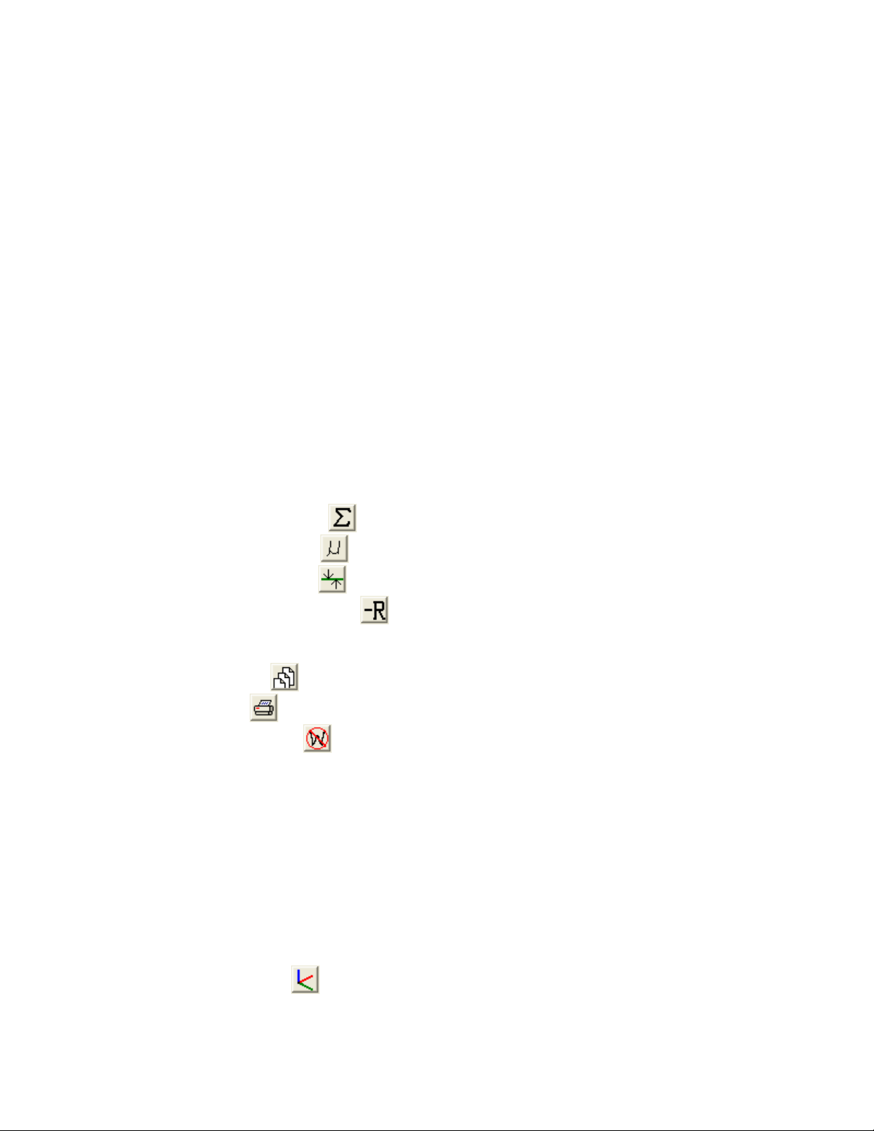
To install your LBA-PC frame grabber card, disconnect the AC power from your computer. Remove
the cover from your computer as described in your computers technical manual. Locate your PCI bus
slots. Most PC’s will have either 3 or 4 PCI slots. Select an unused PCI slot and remove the rear filler
bracket associated with that slot. (See figure below)
Operator’s Manual LBA-PC
Doc. No. 10654-001, Rev 4.10
15
Page 16
Note: If you purchased the optional 4 camera adapter, or the optional digital adapter then make sure that the slot
immediately to the left (viewed from the front of your PC) of the above PCI slot is also empty, and remove its rear
filler bracket also.
Figure 1
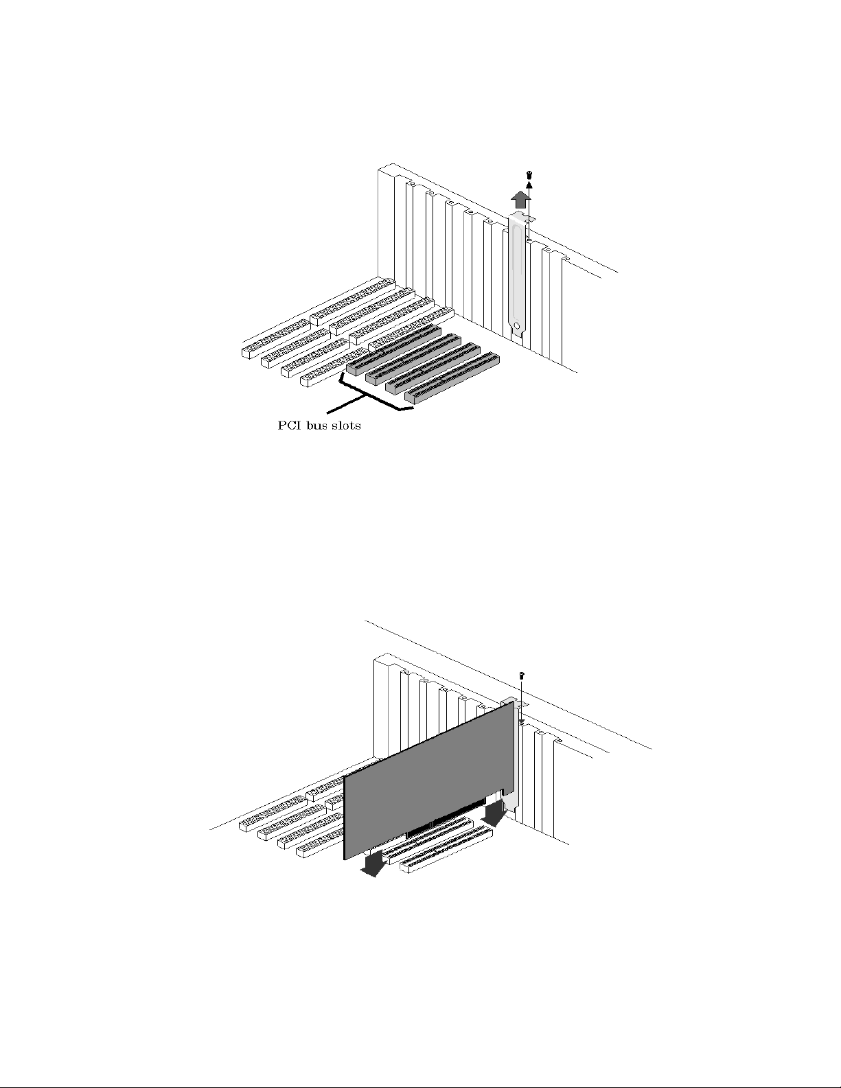
Carefully plug your LBA-PC frame grabber card into the PCI slot. Make sure that it is fully seated in
the PCI connector. Secure the end bracket with the screw that held in the filler plate. (See figure
below)
Figure 2
Operator’s Manual LBA-PC
16
Page 17
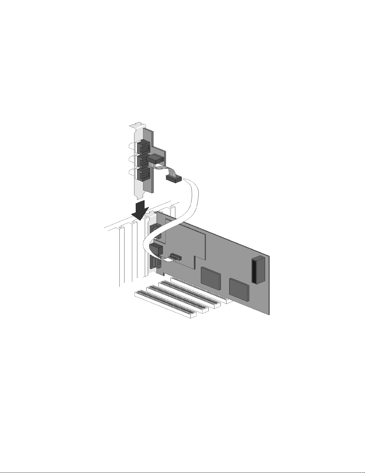
The optional adapters use the rear panel opening, but do not plug into any of the PC expansion slots. Rather it is
provided with a short ribbon cable that plugs into the frame grabber card. (See figures below) Slide the adapter
into the rear opening and plug its cable into the frame grabber card. Secure the adapter bracket to the rear panel
with the screw that held in the filler plate.
Four Camera Option
Figure 3
Operator’s Manual LBA-PC
Doc. No. 10654-001, Rev 4.10
17
Page 18
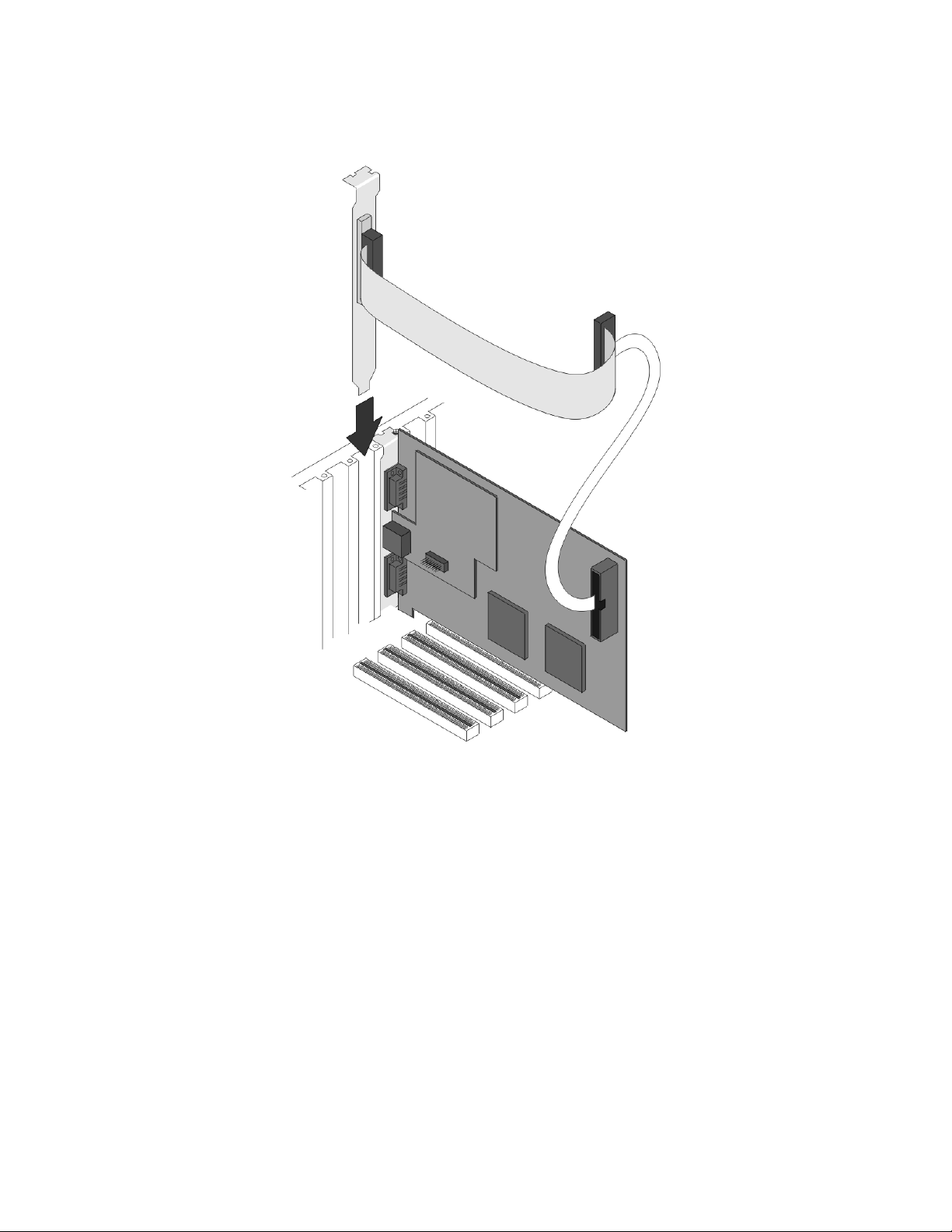
Digital Camera Option
Figure 4
Replace the cover of your computer. Restore the AC power to your computer.
Note: The location of the connectors may vary depending upon which frame grabber model is being installed. The
older LBA-400/500 series has a slightly different arrangement but the concept remains the same.
2.1.2 Step 2 Camera Connections
If you purchased a Pyrocam III to use with LBA-PC, disregard this section and refer to your Pyrocam
III Installation Guide. To use LBA-PC with your Pyrocam III you must launch LBA-PC from the
Pyrocam III Control Console.
Operator’s Manual LBA-PC
18
Page 19

2.1.2.1 Analog Cameras
Connect the video out from your camera to the BNC connector on the LBA-PC frame grabber
card. This is the camera 1 input channel. If you have the 4-camera adapter option, then camera
2’s input is at the top, 3 in the middle, and 4 at the bottom of the adapter bracket assembly.
If you purchased your camera from Spiricon, you may have been provided with a Camera Control
Cable. This cable will usually provide power to your camera, and also control signals for your
camera’s electronic shutter (if it has one). Plug this cable between the appropriate 9-pin
connector on the frame grabber card, and into your camera. If you have the 4-camera adapter,
the additional cameras will need to be powered from an external power supply.
Your camera may also be supplied with a separate power supply. If so, connect it according to
the instructions provided with the camera.
2.1.2.2 Digital Cameras
Connect the digital output from your camera to the SCSI-2 type connector on the digital camera
adapter provided with the LBA-PC frame grabber card. If you purchased your camera from
Spiricon, you may have been provided with a Camera Control Cable. The cable will provide the
digital data connection to your camera, and may control signals for your camera’s electronic
shutter (if it has one).
Your camera may also be supplied with a separate power supply. Connect it according to the
instructions provided with the camera. Digital cameras may require additional software to control
the camera. Check with the camera manufacture and follow their instructions.
2.1.3 Step 3 LBA-PC Software Installation
After the frame grabber is physically installed in the computers PCI slot, and the PC is rebooted,
windows may tell you that it has found new hardware and ask you to install its driver. If this occurs
exit out of the found new hardware wizard without installing a driver and instead allow the LBA-PC
installation application to load the necessary files and drivers. After the installation application has
run, the hardware should be installed properly and you will not see the found new hardware wizard.
If problems do occur during the installation and the drivers are not properly installed, windows will
launch the new hardware wizard after the installation. If this situation should occur, tell the wizard to
search automatically for the necessary drivers, finish the wizard and reboot.
Here are two ways to install LBA-PC in Windows XP; the second method will also work for Windows
2000. Choose only one of the following:
First Method (Windows XP):
Step 1) Start Windows.
Step 2) Close all other Windows applications.
Step 3) Place the Spiricon CD into your CD-ROM drive.
Step 4) Windows XP will open a dialog that asks: “What do you want Windows to do?”
Step 5) Click “Open folder to view files”! Windows will open a folder in the CD’s root directory
showing folders for each of the shipped Spiricon applications.
Step 6) Double click the “LBA-PC” folder to open it.
Operator’s Manual LBA-PC
Doc. No. 10654-001, Rev 4.10
19
Page 20

Step 7) Double click the file in the LBA-PC folder named “Setup.exe” to launch the install. (The
windows file extensions, for this folder, must be set to viewable to see the “exe”
extension.)
Step 8) Follow the instructions in the installation dialogs.
Step 9) Reboot when installation is complete.
Step 10) LBA-PC should now be installed.
Second Method (Windows 2000 or XP):
Step 11) Start Windows.
Step 12) Close all other Windows applications.
Step 13) Place the CD in the CD-ROM drive
Step 14) Click Cancel when Windows asks you, “What do you want to do?
Step 15) From the Taskbar, click on Start, and then Run…
Step 16) In the Open line type: R:\LBA-PC\setup.exe and press <Enter> (Where “R” is the letter
of your CD-ROM drive).
Step 17) Follow the directions given in the installation dialogs.
Step 18) Reboot when installation is complete.
Step 19) LBA-PC should now be installed.
Note: After the installation is completed, The install dialogs will ask you if you want to restart windows, you must
answer yes to allow windows to restart and load the drivers, otherwise LBAPC will not function properly.
Note: Be sure to look at the LBA-PC ReadMe.txt file, before starting the LBA-PC application. This will bring you
up to date with any last minute information regarding the current version of the program.
The following Windows display settings may need adjustment to accommodate the LBA-PC
Application. Use Control Panel, Display, and Settings tab to make these adjustments:
• Screen resolution should be set for a minimum display size of 1024x768, bigger is better.
• Color Quality should be set to a minimum of 256 colors.
2.1.4 Step 4 Start LBA-PC
It’s recommended that you read portions of this operator’s manual to become familiar with the
operation and capabilities of the LBA-PC. The operator’s manual may be found on the installation disk
in PDF format. The PDF may also be found on the Spiricon web site at www.spiricon.com, just
following the LBA-PC product links. To start the Laser Beam Analyzer application go to windows
taskbar and select:
Start, Programs>, Spiricon>, LBA-PC>, LBA-PC.
Operator’s Manual LBA-PC
20
Page 21

2.1.5 Step 5 Configure Camera Type
You should now have the LBA-PC application window on your monitor. The default configuration is
for a basic CW laser setup. This will allow you to verify that your camera and hardware are operating
correctly. If you received any error or warning messages while starting the LBA-PC application, refer
to the Error Messages section in this chapter before proceeding.
Before you can begin to collect data from your camera you must select the correct camera type. To
do this click Options, Camera..., and then click on the Camera drop down arrow. Select the
camera type that matches (or most closely matches) your specific camera, then click on OK.
To save this setup configuration... Click File, then Save Config...; enter a file name for this
configuration, then click OK. This file name has now become your new default configuration file.
This default will remain, from one program startup to the next, until you save or restore a new
configuration file; at which time, the last loaded or saved configuration becomes the default.
2.1.6 Step 6 Collect Data
Click the Start! menu item to begin collecting data from the camera. The frame display window
should immediately start changing colors corresponding to the intensity of the light reaching the
camera sensor, and the beam profile displays should change from a flat line in proportion to the light
intensity at the cursors.
If the room light is bright enough and/or the camera is sensitive enough, the frame display window
may be entirely white as the horizontal and vertical profile displays move upward and to the right,
respectively. If this is the case, reduce the amount of light reaching the camera sensor by shading it
with your hand. You should be able to obtain the entire range of colors shown on the color bar along
the right side of the display window. If you are using a camera with a lens, you should be able to
obtain a recognizable image by adjusting the lens f-stop and focus.
2.1.7 Step 7 Sample Configurations
You are probably now ready to try looking at a laser, and to go exploring the many operating options
of the LBA-PC.
CAUTION
Before you expose your camera to your laser beam, make sure that
the power/energy of your laser is well below the damage threshold
of your camera’s photo imager. You may also need to attenuate
your beam to bring it into a range that will prevent your camera’s
imager from saturating.
To help you get started, we have created a set of configuration files that you can restore. These
configuration files will adapt the LBA for a variety of basic operating modes.
However, these configuration files do not know which particular camera you are using. Therefore you
must select the appropriate camera to complete your setup. To select a camera, you will have to
repeat the procedure in Step 5.
Operator’s Manual LBA-PC
Doc. No. 10654-001, Rev 4.10
21
Page 22

The factory-supplied configuration files are write protected, so that you cannot accidentally lose or
overwrite them. Each of these file names begin with a ~ (tilde), for easy identification. Some
examples of these files are:
~lbapc.cfg The original default configuration.
~cw_basc.cfg A CW laser setup w/ basic results.
~cw_gaus.cfg A CW laser setup w/ Gauss Fit results.
~cw_hist.cfg A CW laser setup w/ Histogram display.
~cw_fram.cfg A CW laser setup w/ 8 frame averaging.
~cw_elip.cfg A CW laser setup w/ elliptical results.
~vt_toph.cfg Video trigger mode for a pulsed laser w/ Top Hat results enabled.
~to5gaus.cfg A Trigger Output at 5 Hz to fire a pulsed laser w/ Gauss Fit results.
~PYROCAM.cfg For use with Pyrocam I’s w/o digital camera option.
~PYRODIG.cfg For use with Pyrocam I’s w/ digital camera option.
2.2 Error Messages
The explanations of the following error messages assume that you are Windows savvy. If you find that
after reading an error message’s meaning, you still do not know what to do, then contact Spiricon’s
Service department for assistance.
You may encounter the following error messages:
LBA-PC device driver not found.
LBA-PC set to Off-Line mode
This error usually indicates that your LBA-PC frame grabber is either not installed or is not working. If
the frame grabber card is not detected by Windows then the device driver will not be loaded when the
system starts. This error may also indicate that the device driver was not properly installed. To
determine the cause, do the following:
Windows 2000
• Click on… Start, Settings, Control Panel.
Or for Windows XP
• Click on… Start, Control Panel.
Then for Both
• Double click on the System icon.
• Select the Hardware tab.
• Click on the Device Manager button.
Operator’s Manual LBA-PC
22
Page 23

• Click on the Sound, video and game controllers listing.
• If the LBA-PC frame grabber was detected, and the device driver was not loaded you will see a
category called Unknown in the edit box listing of the Device Manager. If this occurs, double
click on the Unknown icon. You should see an entry called PCI Card. This indicates that the
device driver was not properly installed. To correct this problem, re-install the LBA-PC software.
• If you did not see the Unknown icon, then Windows did not detect the LBA-PC frame grabber
card. Check to see that your frame grabber card is properly installed. Sometimes PCI card slots
are defective, so you might also try another slot if all else seems to be in order.
If this device driver is not found, the LBA-PC program will complete loading, but the software will be
forced to the Off-Line mode. This means you can only view files and perform Post Processing of data
from and/or to data files.
Device Drive vX.XX detected.
LBA-PC requires vY.YY.
LBA-PC set to Off-Line mode.
If your current device driver version does not match the current LBA-PC version you will get this
message. This may occur if you have upgraded your LBA-PC application, but continue to use an old
device driver. Normally this should not happen, as the installation will install a new device driver
version with each upgrade. The LBA-PC application program will complete loading, but the software will
be forced to the Off-Line mode. This means you can only view files and perform Post Processing of
data from and/or to data files.
Unable to load LCA program file.
File Not Found.
This message will precede the following error message if the lcaXXX.exo file is not found or is not in the
same path as the LBA-PC application.
LBA-PC frame grabber
detected, but cannot initialized.
LBA-PC set to Off-Line mode.
The LBA-PC frame grabber contains a programmable LCA device. If this device fails to program during
application initialization, the above error message will occur. Contact the Spiricon Service Department
for assistance. The LBA-PC application program will complete loading, but the software will be forced
to the Off-Line mode. This means you can only view files and perform Post Processing of data from
and/or to data files.
Not Enough Memory for Frame Capture.
LBA-PC set to Off-Line mode.
Operator’s Manual LBA-PC
23
Doc. No. 10654-001, Rev 4.10
Page 24

The device driver was unable to allocate enough memory in order to capture video frames. This may
occur the first time you boot the computer after installing the Frame Grabber card. Try rebooting the
computer. If the error continues to occur you will need to add memory to the computer. LBA-PC
requires a minimum 256 MB of main memory, 512 MB is recommended. If the error occurs after
adding memory then contact the Spiricon Service Department.
Frame Grabber not found.
LBA-PC set to Off-Line mode.
Your LBA-PC frame grabber card is either not installed, or not working. The LBA-PC application
program will complete loading, but the software will be forced to the Off-Line mode. This means you
can only view files and perform Post Processing of data from and/or to data files. Check to see that
your Frame Grabber card is properly installed. Contact the Spiricon Service Department for further
assistance.
Not a valid LBA-PC data file.
You are attempting to load a file that is not in a format that the LBA-PC can recognize. See loadable
file types.
2.3 Optional Equipment
Optional equipment can include the following items:
License: Multi-user site software license
Adapter: 4 Camera adapter
Digital Camera adapter
Camera: Selected camera, specify type
Interface cable
BNC cable
Camera manual (if supplied by camera manufacturer)
Camera power supply (if supplied by camera manufacturer)
Computer: PC compatible, Pentium or equivalent
Attenuator: Model LBS-100, BA-VIS, -NIR, or -BB beam attenuator
2.4 Connections
This topic describes the Camera Control (upper, 9 pin D-sub, female) and Trigger I/O (lower, 9 pin Dsub male) connectors on the LBA-PC rear panel. The schematic shown below describes the circuits on
these connectors. See the Specifications section for the respective drive limits of these signals.
Operator’s Manual LBA-PC
24
Page 25
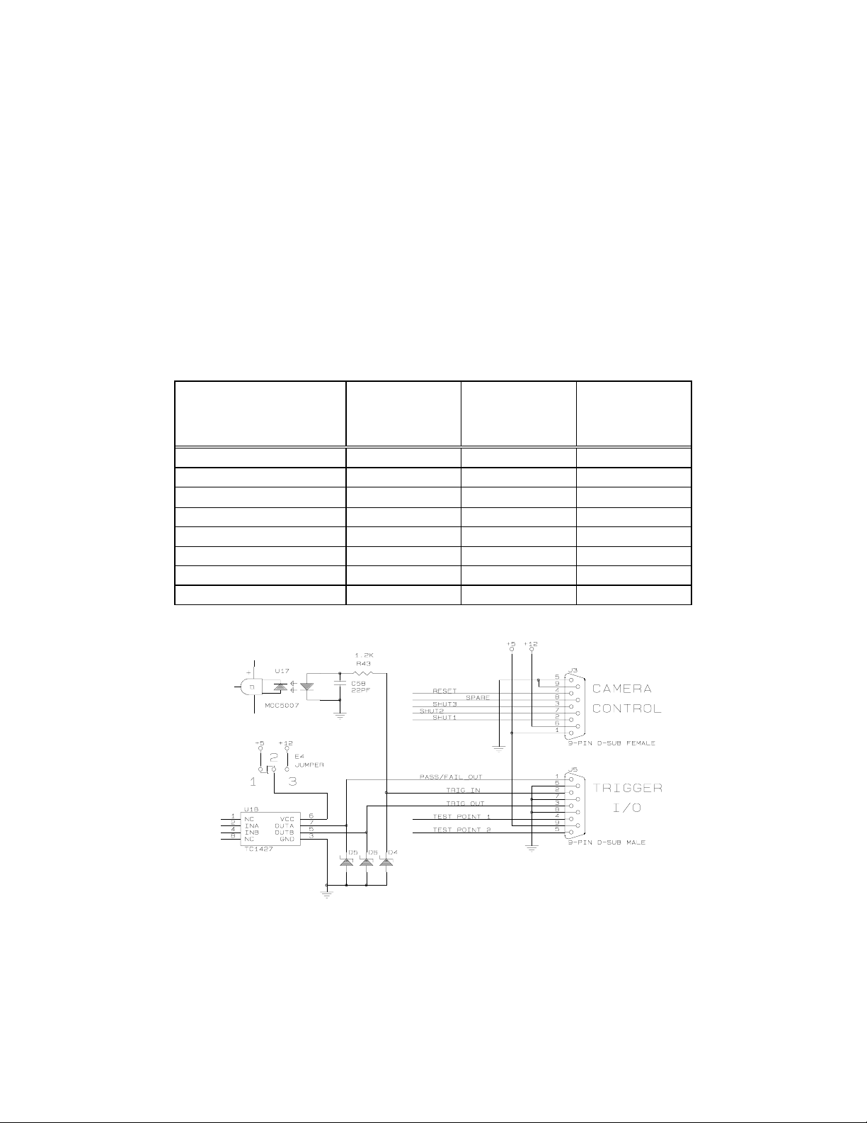
2.4.1 Camera Power
If your camera is a low power CCD style that runs on +12Vdc, then it may be powered from
connector J1 (J3 on LBA-3/4/500 frame grabbers) pin 6 (+12Vdc) and pin 5 (gnd).
Caution: Do not attempt to power more than ONE camera from the LBA-PC.
2.4.2 Shutter Controls Signals
The electronic shutter control signals are provided on as SHUT1, SHUT2, and SHUT3. These are TTL
level drive outputs. The Logic is positive true. The shutter settings are listed in the 8 lines of the
Shutter drop down edit control found in the main menu Options > Camera > Advanced dialog
box. The labeling of the shutter lines can be user modified to match the settings of a particular
camera. The line locations however, always correspond to the following TTL output drive levels:
Shutter Line
Edit control
Top line 1 0 0 0
2 0 0 1
3 0 1 0
4 0 1 1
5 1 0 0
6 1 0 1
7 1 1 0
Bottom line 8 1 1 1
SHUT3
(J1 pin 3)
(J3 on 3/4/500)
SHUT2
(J1 pin 7)
(J3 on 3/4/500)
SHUT1
(J1 pin 2)
(J3 on 3/4/500)
Frame Grabber Pin-out
Figure 5
Operator’s Manual LBA-PC
Doc. No. 10654-001, Rev 4.10
25
Page 26

2.4.3 Trigger Out
Connector J2 (J5 on LBA-3/4/500 frame grabbers) pin 3 is the Trigger Out signal. This signal is factory set to output +5Vdc pulses. You can change this signal to +12Vdc level pulses by moving Jumper E1 (E4 on LBA-3/4/500 frame grabbers) to bridge pins 2-3.
Note: Jumper E1 (E4) controls the output signal level for both Trigger Out and Pass/Fail Out. Jumper position 1-2
yields a +5Vdc level; position 2-3 yields a +12Vdc level.
2.4.4 Pass/Fail Out
Connector J5 (J2 on LBA-7XX frame grabbers) pin 1 is the Pass/Fail Out signal. This signal is factory set to output +5Vdc pulses. You can change this signal to +12Vdc level pulses by moving Jumper E1(E4) to bridge pins 2-3. To enable this signal and select its mode of operation see the Pass/Fail menu topic.
Note: Jumper E1 (E4) controls the output signal level for both Trigger Out and Pass/Fail Out. Jumper position 1-2
yields a +5Vdc level; position 2-3 yields a +12Vdc level
.
2.4.5 Trigger In
Connector J2 (J5 on LBA-3/4/500 frame grabbers) pin 2 is where you apply the Trigger In signal. This input must be only a positive voltage with respect to ground. But you can pulse it with either a high going or a low going pulse. You can program the Trigger In Polarity to respond to either a positive (rising) or negative (falling) edge of this input signal.
2.4.6 Video In
The BNC connector (not shown above) is where you input either RS-170 or CCIR formatted black and
white video. The video input is terminated into 75 ohms. This is Camera input number 1. If you
have purchased the 4 camera option, three additional BNC connectors are provided on a separate
bracket assembly. These BNC connectors provide inputs for cameras number 2, 3 and 4 (top to
bottom).
2.5 Camera Control Cables
Many cameras shipped by Spiricon will be supplied with a Camera Control Cable. Connect this cable
between the camera and connector J1, (J3 on LBA-3/4/500 frame grabbers) the upper 9-pin D-sub
female. This cable will usually provide power to the camera, as well as permit the LBA-PC to control a
camera’s electronic shutter, if it has one. Cameras that derive power from a source other than the LBAPC will not usually be supplied with this cable.
If you are using the 4-camera option, any additional cameras must be powered from an external
source. To provide control of the shutter of any additional cameras, a special cable must be made that
connects all of the shutter inputs of the cameras in parallel. If you plan on using the automatic camera
sequencing you may also need a special cable to synchronize (genloc) the cameras.
Operator’s Manual LBA-PC
26
Page 27

2.6 Special Setup for Pyrocam I Operation
You must use special setups if you want to successfully interface your Pyrocam I with a Model LBA-PC
frame grabber system. It is strongly recommended that you first become familiar with the operating
characteristics of both your Pyrocam I and LBA-PC before attempting to operate them together.
To operate your Pyrocam I with a model LBA-300PC or a LBA-400/500/708/710/712/714PC without a
digital camera option, see section 2.12.1.
To operate your Pyrocam I with model LBA-500PC-D or a model LBA-7XXPC-D, with the digital camera
option, see section 2.12.2.
2.6.1 Pyrocam I with Non-Digital LBA-PC’s
LBA-300/400/500/708/710/712/714PC w/o digital camera option
2.6.1.1 Pyrocam I Setup Requirements:
2.6.1.1.1 Configure Video Output
The Pyrocam must be configured to output monochrome video in CCIR format. To do this,
Dip Switch number 6 must be in the ON position. See Chapter 6 and Appendix A-6 in your
Pyrocam Operator’s Manual for details.
2.6.1.1.2 Configure Gain and Vertical Scale
Do not operate the Pyrocam I with the Gain switch set in the 10 position or with the
Vertical Scale set in the Auto or Manual x8 positions. Use only the 1 or 3 Gain setting and
Manual x1, x2 or x4 settings. The LBA will not be able to Ultracal in the gain equals 10 or
scale x8 setting positions, and the Ultracal will not remain valid if the Pyrocam is in the Auto
scale mode.
Note: You will need to temporarily attach your Pyrocam to either a VGA or a monochrome monitor to observe the
Vertical Scale settings.
2.6.1.1.3 Configure MONO/DIG/VGA switch to MONO position.
2.6.1.1.4 Install Video Cable
Connect the Pyrocam’s Video Output BNC to the Video Input BNC on the LBA-PC.
All other operating requirements for the Pyrocam I are still applicable, and must be set up
correctly. Don’t forget to periodically calibrate your Pyrocam.
Hint: First set up your Pyrocam to operate in one of its stand-alone configurations, and then connect it to the LBAPC only after you’re sure that it is operating satisfactorily with your laser.
Operator’s Manual LBA-PC
Doc. No. 10654-001, Rev 4.10
27
Page 28

2.6.1.2 Setup requirements for LBA-PC with pyrocam cameras:
Two files are provided for configuring the LBA to a Pyrocam I. They are ~PYROCAM.CFG and
~PYROCAM.CAM.
2.6.1.2.1 Setting up the Pyrocam Configuration.
Go to File. . . Restore Config. . . and set the configuration to ~PYROCAM.CFG.
2.6.1.2.2 Setting the camera type to Pyrocam
Go to Options. . . Camera dialog box and set the Camera selection to ~PYROCAM.CAM.
This may already have happened when you did the previous step.
The ~PYROCAM.CAM file is absolutely required for correct operation with your Pyrocam. The
~PYROCAM.CFG configuration is a good starting point configuration.
You will undoubtedly need to make changes to your configuration to suit your application.
Do so, and then save off your new configurations into new <filename>.cfg config files.
Remember the ~PYROCAM files are read only; so don’t try to use those file names.
2.6.1.3 Some Restrictions apply when interfaced to a Pyrocam I
2.6.1.3.1 Frame resolution restrictions
While you are not restricted from setting your frame Resolution to 512x480x1, it is not a
good idea. Keep your Resolution setting set to 128x120x4. Remember the Pyrocam creates
a 124x124 sized image, so setting higher resolutions only wastes memory and slows down
operations.
2.6.1.3.2 Zooming restrictions
In keeping with the above, do not use Hardware zooming. Only use Soft zooming, i.e.
double-right-mouse click in the Zoom window.
2.6.1.3.3 Restricted pixel regions
Because of the image size difference between the LBA and the Pyrocam I, as noted above,
the LBA will clip off 4 rows from the Pyrocam; two on top, and two on the bottom. Also the
LBA will have 4 dark columns; two on the left edge, and two along the right.
2.6.1.3.4 Scale and resolution restrictions
Note also that the Pixel Scale setting is set to 25mm, not 100mm, which is the actual pixel
scale of the Pyrocam I. This is because the image output by the Pyrocam in CCIR mode is 4
times over scanned in both the x and y directions. Thus the LBA’s 1x resolution comes out to
be 1/4th the 4x resolution. Keep this in mind if you plan to change the scaling because of
placing the beam altering optics in the beam path.
Operator’s Manual LBA-PC
28
Page 29

2.6.1.3.5 Camera settings restrictions
Under no circumstances, make any changes to the Advanced. . . Camera settings for the
Pyrocam I.
2.6.1.4 Image synchronization considerations
The Pyrocam I’s CCIR video output is always producing video images at the rate of 25 frames per
second. Furthermore, it only changes output image after acquiring and processing a new image.
Thus the rate of a new output beam image is a function of many variables, including Pulse or
Chop rates, image processing time, and results computational times.
If you are using a Pulsed laser with your Pyrocam I, the Pyrocam will continue to output the
image of the last laser pulse that it receives. As a result, your LBA will continue to collect data
frames that are multiples of the last pulse received by the Pyrocam. To relieve this, you may
want to set up a Trigger input to the LBA. This will cause, at the most, only one image to be
acquired for each Laser Pulse. This can be a tricky situation since the Pyrocam does take a little
time to process each image, and that time will vary somewhat from image to image. Also, if your
laser is triggered faster than the Pyrocam can acquire and update its CCIR display, it will skip
pulses. Thus the LBA can still end up acquiring multiples of some of the processed pulses. You
can also try the solution described below for the Chopped-operating mode.
The exact same type of problem occurs in Chopped mode. The chop frequencies must be either
24Hz or 48Hz. Thus, the CCIR image can never be updating as fast as the chopper is triggering
the Pyrocam. Consequently, the CCIR output is always creating multiple frames of the same
beam profile. In this case, you may want to set the LBA’s Capture interval to a value that will
eliminate or reduce multiple frame captures.
2.6.2 Pyrocam I with Digital LBA-PC’s
LBA-500/7XXPC-D w/ Digital Camera Option
2.6.2.1 Pyrocam I setup requirements:
To use this interface method, your LBA-500/7XXPC must be equipped with the digital camera
option (-D), and your Pyrocam I must be of a later design that has digital output capability. Early
versions of the Pyrocam were not equipped with digital outputs. If your Pyrocam I does not have
a 50 pin connector on its rear cover it can not be interfaced as a digital camera. However, you
can still interface it by using the analog method described in the LBA-300PC interface topic.
Alternately, you can contact Spiricon’s service department and arrange to have your Pyrocam I
upgraded with digital camera output capability.
NOTICE: When interfacing with a Pyrocam I, DO NOT USE THE ULTRACAL! Feature of the LBA-PC. Rather, it
is ESSENTIAL that you periodically re-calibrate the Pyrocam I. Calibrating the Pyrocam I is the only calibration
that should be used with this type of interface.
Operator’s Manual LBA-PC
Doc. No. 10654-001, Rev 4.10
29
Page 30

2.6.2.1.1 Set video switch
The Pyrocam must be set to output digital video. This is accomplished by setting the
MONO/DIG/VGA switch to the LBA position. See Chapter 6 in your Pyrocam Operator’s
Manual.
2.6.2.1.2 Connect cable
Connect the Pyrocam’s digital output to the digital input connector of the LBA-500PC. A
special interface cable is required to make this connection. If you ordered your Pyrocam I,
LBA-PC and LBA-Digital Option together as a system, then a cable was supplied.
2.6.2.1.3 Pyrocam settings
With the Pyrocam set to the DIG mode, the Vertical Scale setting has no effect on the
output. However, the Gain switch is still operating and can be set to any position. All other
operating requirements for the Pyrocam I are still applicable, and must be set up correctly.
Don’t forget to periodically Calibrate your Pyrocam.
Hint: First set up your Pyrocam to operate in one of its stand-alone configurations, and then connect it to the LBAPC only after you’re sure that it is operating satisfactorily with your laser.
2.6.2.2 LBA-500/7XXPC-D Setup requirements:
Two files are provided for configuring the LBA-PC digital interface to a Pyrocam I. They are
~PYRODIG.CFG and ~PYRODIG.CAM.
2.6.2.2.1 Set the Pyrocam configuration
Go to file. . . Restore Config. . . and set the configuration to ~PYRODIG.CFG.
2.6.2.2.2 Set the camera options
Go to Options. . . Camera dialog box and set the Camera selection to ~PYRODIG.CAM.
This may already have happened when you did the previous step.
The ~PYRODIG.CAM file is absolutely required for correct operation with your Pyrocam. The
~PYRODIG.CFG configuration is a good starting point configuration.
You will undoubtedly need to make changes to your configuration to suit your application.
Do so, and then save off your new configurations into new <filename>.cfg config file.
Remember the ~PYRODIG files are read only, so don’t try to use those file names.
Under no circumstances make any changes to the Advanced… Camera settings for the
Pyrocam I.
Operator’s Manual LBA-PC
30
Page 31

2.6.2.3 Image Synchronization Considerations
The Pyrocam I’s Digital Output only produces an image each time new data is available. It will
not continuously output the same frame repeatedly. Thus, the rate of new output beam images
is a function of the Pulse or Chopping rate and image processing time. For this reason, you
should operate the LBA-500PC in Video Trigger mode only.
If you are using a Pulsed laser with your Pyrocam I, the Pyrocam will attempt to output a new
image with each laser pulse, however, depending upon the pulse rate, it may not be able to keep
up.
The exact same type of problem occurs in Chopped mode. The chop frequencies must be either
24Hz or 48Hz. The Pyrocam may be able to keep up at 24Hz, but will lose some frames at 48Hz.
Operator’s Manual LBA-PC
Doc. No. 10654-001, Rev 4.10
31
Page 32

Chapter 3 MENUS AND DIALOG BOXES
3.1 File. . . Drop Down Menu Selections
3.1.1 File | Load. . .
A saved data file can be loaded into the frame buffer for display and results processing. Four types of
data file formats are supported and are delineated by their file extension labels. The results obtained
from these file types are not all of equal merit, however. The origin and meaning of these file types
are as follows:
.lb3/4/5/7 Files
Is the native file extension denoting a data file created by the LBA-PC. The number indicates
that the data was created by either the LBA-300 (8-bit frame grabber), -400 (10 bit frame
grabber), –500 (12 bit frame grabber), or with a new –7XX (multi-format frame grabber). If the
saved file was generated using Ultracal processing then the results obtained when loading and
viewing this file type are of high quality.
.lba Files
Is the native file extension denoting a data file created by the LBA-100A. If the saved file was
generated using Autocal processing then the results obtained when loading and viewing this file
type are of high quality. All of these files produce images that are 120 x 120 pixels.
.lbb Files
.lbc Files
Is the native file extension denoting a data file created by the LBA-100A. All file types of this
designation are created without the benefit of any calibration, and thus can not be relied upon
for accurate results. All of these files produce images that are 256 x 240 pixels.
Is the native file extension denoting a data file created by the LBA-100A. All file types of this
designation are created without the benefit of any calibration, and thus can not be relied upon
for accurate results. All of these files produce images that are 512 x 480 pixels.
NOTICE:
File Compatibility with New versions of LBA-PC Software.
We will try very hard to make all future releases of the LBA-PC
application backwards compatible with all prior .lb3/4/5 file
formats. However, we cannot guarantee that new versions will
produce .lb3/4/5 files that will be backward compatible with older
versions.
Operator’s Manual LBA-PC
32
Page 33
Beginning with release v2.50, any of the three .lb3, .lb4, and .lb5
file types can be read by any of the LBA-300/400/500PC model
types. However, the new .lb4 and .lb5 file types cannot be read by
software released prior to v2.5.
Beginning with release v4.00, any of the three .lb3, .lb4, and .lb5
file types can be read by any of the LBA-7XXPC model types.
However, the new .lb7 file types cannot be read by software
released prior to v4.00.
Data files can contain one or more frames of data. Each frame of data is called a Record.
Embedded in each Record is all the information necessary to accurately reproduce the original frame.
Pixel scale, Camera type, Zoom and Pan location, energy and Ultracal values etc. are saved within
each Record.
Note: If you load an LBA-100A record that used a different camera setup than the one you currently have
configured, then one or more of the following can occur:
• If the Camera type file is available, it will be loaded and replace the current settings. See Camera
type selection.
• If the Camera type file is available, but the pixel scale or resolution settings do not agree with the
current settings, it will be loaded and the Pixel Scale and Resolution settings changed to match
the data file values.
• If the Camera type file is not available, the camera type will be set to NONE, and the Pixel Scale
and resolution will be changed to that required of the Data File.
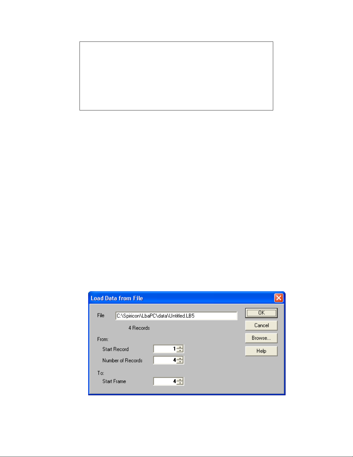
3.1.1.1 Load Frame Dialog Box
Enter the drive:\paths\and <filename>.lbx of the File that you want to load. Press Browse... if
your not sure of the file’s name or location, and wish to search for it.
Figure 6
Operator’s Manual LBA-PC
Doc. No. 10654-001, Rev 4.10
33
Page 34

If the file that you are loading contains multiple records, enter the starting number of the record
that you want to begin loading from, in the edit box labeled Start Record.
Enter the Number of Records that you want to Load. You can enter a value of 0, or 1 to the
number of records in the file. A value of 0 means all the records in the file.
Records can only be loaded sequentially from the Start Record position. If you specify a
greater number of records than you have frame buffer space available, the loading process will
fill the buffer and then wrap around leaving the last records transferred in the frame buffer. See
setting the frame buffer size in 3.2.3.4.
In Start Frame, enter the location in the frame buffer where you wish to begin depositing the file
records. Multiple frames will load from that location upward, skipping any locations that are
Write Protected.
3.1.1.2 Special Frame Numbers
The following Frame numbers have special meanings, however they can be saved and loaded in
the usual manner.
• Frame 0 is the Reference Frame
• Frame -1 is the Gain Correction frame, not a true image frame, but rather an array of
gain correction factors.
3.1.1.3 Drag and Drop Data Frame Loading
You can perform a Load Frame operation by dragging and dropping one or more data frame files
from Windows Explorer, or by double clicking the data file name. If you have not already
started the LBA application, using the double click method will start it automatically.
These Drag and Drop shortcuts will work on all Data Frame formats. However, the current
camera configuration must match the camera configuration of the data file that you are
attempting to load. If you Drag and Drop a data file that contains multiple records, all the frame
records will be loaded into the frame buffer up to the maximum size of the buffer. For example:
If you Drag and Drop a file with 20 records, and your frame buffer is sized at 10 frames, then
only the first 10 records in the data file will be loaded.
To perform a Drag and Drop, open Windows Explorer. Highlight the data file(s) that you want
to load. With the Mouse cursor over the file name, press and hold down the left mouse button
while dragging the highlighted files to the LBA-PC application.
3.1.2 File | Save As…
You can save or append data frames in the frame buffer to disk files. All data files saved by the LBAPC will have a .lb3/4/5/7 file name extension.
Data files can contain one or more frames of data. Each frame of data is called a Record.
Embedded in each Record is all the information necessary to accurately reproduce the original frame.
Pixel scale, Camera type, Zoom and Pan location, energy and Ultracal values etc. are saved within
each Record.
Operator’s Manual LBA-PC
34
Page 35

3.1.2.1 Save As … Dialog Box
Enter the drive:\paths\<filename> of the File that you want to save. Press Browse... if you
want to append or overwrite an existing file, and you are not sure of the file’s name or location
and wish to search for it.
Figure 7
Enter the Start Frame buffer location from which you want to begin saving or appending frame data
files.
If you wish to save multiple records, enter the Number of Frames that you want to save or append.
Multiple data frames can only be saved sequentially from the Start Frame location. You can specify
0, or 1 to the number of frames in the frame buffer. A value of 0 means all of the frames in the
frame buffer.
3.1.3 Export Image… to a disk file
Exporting is an operation that is designed to take data and images out of the LBAPC and use them in
other applications. Exports are a bad choice for data storage because there is no way to reload
exported data into the LBA-PC! Bitmaps for example, are one of the exporting options. Bitmaps
(.bmp) are simply pictures of the beam image and do not represent a viable data source for numerical
analysis. If the user desires to do some external computations on exported data, ASCII formats have
been provided and are the only viable method for doing so.
Bitmap images will appear just as the current beam display window image appears. The two ASCII
file types are .cma and .spa. The .cma type uses Comma delimited entries. The .spa type uses
Space delimited entries. Spreadsheet programs like Excel and Lotus 123 typically use comma
delimited data entries. Math programs like Mathcad typically use space-delimited formats. Consult
your application program to determine which style to use.
You can also save 1D beam display images that are defined by the location of the Horizontal and
Vertical Cursors. Cursor files are designated with a .cur file type. Cursor files are ASCII files that
use Comma delimited entries. The Cursor image is organized Horizontal data first, left to right,
followed by a carriage return, and then the Vertical data, top to bottom.
You can also save a Column and Row summed beam image that is defined by the total of all
pixel values summed in both the Horizontal and the Vertical direction. Column/Row summed files
are designated with a .sum file type. Summed files are ASCII files that use Comma delimited
Operator’s Manual LBA-PC
Doc. No. 10654-001, Rev 4.10
35
Page 36
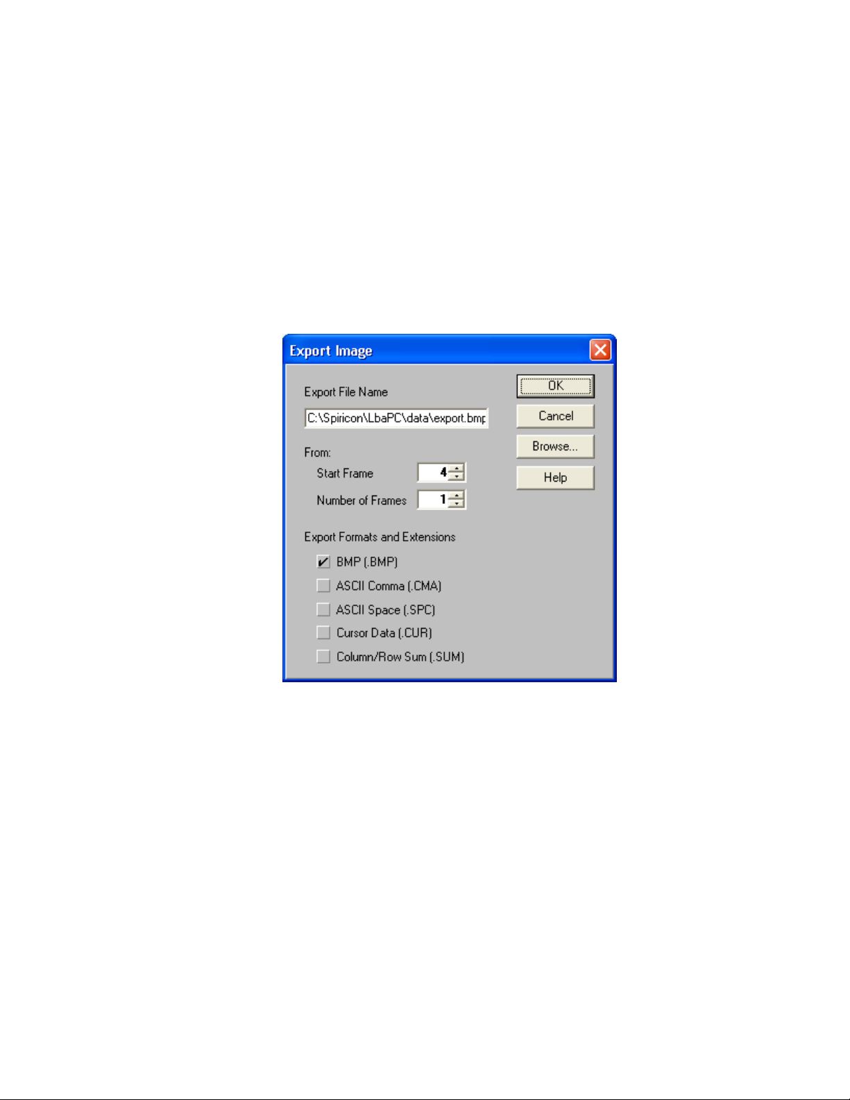
entries. The Summed image is organized Horizontal data first, left to right, followed by a carriage
return, and then the Vertical data, top to bottom.
Note: Exported image files cannot be read back into the LBA-PC’s frame buffer. Use Save As... and Load... for
retrievable data files.
3.1.3.1 Export Image… dialog box
Enter the drive:\paths\and <filename> of the Export File Name that you want to create. Press
Browse... if you want to overwrite an existing file, and you are not sure of the file’s name or
location and wish to search for it.
Figure 8
Enter the Start Frame buffer location from which you want to begin exporting image data files.
If you wish to save multiple images, enter the Number of Frames that you want to export.
Multiple export images can only be saved sequentially from the Start Frame location. You can
specify 0, or 1 to the number of frames in the frame buffer. 0 means all the frames in the frame
buffer.
When Exporting multiple images, each image will be placed into a separate file. The file name
will automatically have a six-digit number appended to the entered file name. This number will
designate each file in the sequence starting with 000000 and counting up. Thus a given multiple
export will create a series of files that will appear as follows:
Operator’s Manual LBA-PC
36
Page 37
<filename>000000.cma;<filename>000001.cma;...<filename>NNNNNN.cma
Click on the image file Export Format (or Formats) that you want to generate.
3.1.4 Save Config… to a file
The current setup configuration of the LBA-PC can be saved to a disk file. All configuration files have
the .cfg file extension. Whichever configuration was the last to be saved (or restored), will become
the default configuration the next time the LBA-PC application is run. The configuration file contains
all setup parameters of the LBA-PC menus.
The configuration file does not preserve and thus will not restore Data frames, Reference frames, Gain
Correction frames, or Ultracal processing information. The above types of frames must be saved and
restored separately. Ultracal processing data must be generated immediately prior to the acquisition
of new data frames, as it relates to present camera calibration requirements.
3.1.5 Restore Config… from a file
Past setup configurations of the LBA-PC can be restored from previously saved .cfg disk files. All
configuration files have the .cfg file extension. Whichever configuration was the last to be restored
(or saved), will become the default configuration the next time the LBA-PC application is run. The
configuration file contains all setup parameters of the LBA-PC menus.
The configuration file does not preserve, and thus will not restore, Data frames, Reference frames,
Gain Correction frames, or Ultracal processing information. The above types of frames must be saved
and restored separately. Ultracal processing data must be generated immediately prior to the
acquisition of new data frames, as it relates to present camera calibration requirements.
Notice: Restoring a configuration does not force a read of a <camera>.cam camera type file. Rather it restores the
Camera dialog box settings, just as they where when the configuration file was created.
3.1.6 Set Reference, copy the current to the reference frame
Set Reference
Click on this button, to copy the Current Frame or the Gauss fit results of the current frame to the
Reference frame buffer. The Reference frame is frame number 0 (zero), in the frame buffer. You
can view the reference frame by single or double clicking into the Frame indicator/edit control
(located in the lower status bar) and entering a 0 (zero). You cannot bring the
reference frame into view by cycling the Frame spin controls.
The Set Reference Source item in the Capture dialog box determines the style of the Save
Reference data.
Operator’s Manual LBA-PC
Doc. No. 10654-001, Rev 4.10
37
Page 38

3.1.7 Generate Gain
Clicking this item will cause the LBA-PC to execute an automatic Gain Correction calculation cycle.
The results of this operation will store a gain correction table that will be used to preprocess all data
frames newly acquired from the Frame Grabber card.
The status of the Gain Correction condition is visible in the Gain correction Enunciator shown here
and at the bottom of the LBA-PC’s main display screen.
If the color of the Gain Correction Enunciator is:
GRAY Gain Correction processing is turned OFF.
GREEN The Gain Correction calculation was successful and is OPERATING.
RED Gain Correction processing has been disabled because something caused the usage of it
to become invalid.
3.1.7.1 How to generate gain
Before clicking on the Generate Gain... item you must:
• Allow the camera to warm up to a normal operating temperature.
• Align your laser beam with the camera and set the correct Zoom, Pan Camera type and
resolution, etc. settings.
• Block all light from the detector and perform an Ultracal!.
• Uniformly illuminate the camera detector to an intensity level that is about 60% to 90%
of saturation.
Now click File, Generate Gain.
• After a few seconds.. observe that the Gain Correction enunciator turns Green.
• Remove the uniform illumination and re-apply your laser beam to the camera.
Note: It is highly recommended that you perform a Save Config... and a Save Gain As... operation in
conjunction with each Generate Gain... operation. This will insure that you can restore the settings to the
configuration that will allow the Gain Correction to operate correctly.
3.1.7.2 What is Gain Correction?
The gain correction algorithm will compute a mean pixel intensity value, and then supply a
correction factor for each pixel that will correct it to the computed mean. If your camera has
dead or seriously defective elements you should not attempt to use or operate with Gain
Correction.
3.1.7.3 What Disables Gain Correction?
Gain Correction will become DISABLED if certain data collection conditions, that were in effect
when the Generate Gain operation was executed, are no longer in effect. In all cases, these
conditions are the result of an operators change to the spatial acquisition settings. The
DISABLED condition will occur if you make changes to:
Operator’s Manual LBA-PC
38
Page 39

• The Hardware Zoom.
• The Hardware Pan location.
• The Camera Type or Resolution setting.
• The Camera Electronic Shutter setting.
• The Video Gain and/or Black Level settings.
Warning: Gain Correction should be used with only one camera at a time. It will not correctly operate in
conjunction with the for camera option when automatic camera cycling is enabled.
3.1.8 File | Load Gain…
You can restore a previously saved .gai Gain Correction file from disk. The Gain Correction enunciator
will turn GREEN if the loaded file will operate under the current setup conditions. If it cannot operate
under the current setup conditions, it will show RED.
Note: It is highly recommended that you perform a Restore Config... on a .cfg configuration file that was saved
at the same time that the .gai Gain Correction file was created. This will insure that you can restore the settings to
the configuration that will allow the Gain Correction to operate correctly.
3.1.9 File | Save Gain As…
You can save the current Gain Correction table to a file. All gain correction files will have a .gai file
name extension. You will not be able to save the Gain Correction table unless you have previously
created it using Generate Gain.
Note: It is highly recommended that you perform a Save Config... and a Save Gain As... operation in
conjunction with each Generate Gain... operation. This will insure that you can restore the settings to the
configuration that will allow the Gain Correction to operate correctly.
3.1.10 Gain Off/On
Click on this button to turn Gain Correction processing OFF or ON. This item will only operate if a
Gain Correction table is present. For a Gain Correction table to be present it must have been created
by Generate Gain, or by being loaded from a disk file via Load Gain.
3.1.11 File | Logging...
The LBA-PC will allow you to log into disk files, in any combination, any of the following:
• Frame Data
• Numerical Results
• Frame Export Images
Data Logging files will have a .lb3/4/5/7 file extension name. The frames in a Data Logging file can
be read back into the Frame buffer by using the File and Load... menu selections.
Operator’s Manual LBA-PC
Doc. No. 10654-001, Rev 4.10
39
Page 40

Results Logging files will have a .rlg file extension name. Results Logging files are for exporting
numerical results to other applications, such as Spreadsheets or Math programs. Text editors can also
view them. Results files are saved in ACSII.
Export Logging files can be of four different file types, .bmp, .cma, .spa, .cur. Export Logging files are
write only. They are created for logging images for use in other applications like spreadsheets or
math programs such as MathCAD. Unlike the .lbx Data file types, Export Logging creates multiple files
rather than one large concatenated file with multiple records. The assigned file name will
automatically have a six-digit number appended to the entered file name. This number will designate
each file in the sequence starting with 000000 and counting up. Thus, an Export Logging operation
will create a series of files that will appear as follows:
<filename>000000.cma; <filename>000001.cma; … <filename>NNNNNN.cma
3.1.11.1 Beginning and Terminating Logging
You begin a logging file when you go to the Logging... dialog box and:
• Check a type of logging
• Provide a file name
• Click on OK
• Click on Start!
You terminate a logging file when you Stop! collecting frames and:
• Return to the Logging dialog box
• Uncheck the logging type
• Click on OK
Warning: Once you have begun a logging cycle, each file entry is sequentially recorded until you terminate the log
via the method described above. If you Stop! and then re-Start! the logging process, the new entries will continue to
be added as before; HOWEVER, the Frame counter or the Timer (whichever might apply) will be reset to 0 (zero)
each time you press Start!. In Export Logging, the file frame numbering does not reset, but rather continues to
increment from the last number assigned. This number is only reset each time logging is enabled.
Example: If you were setup to log 1000 frames, and you hit Stop! at frame 521, and then hit Start! a second time;
when the logging process stops automatically, the log file will contain entries for 1521 frames.
3.1.11.2 Data, Results & Export Logging, dialog box
If you want to log frames of data, check the Data Logging box and enter the
drive:\paths\<filename> of where you want the data records to be logged.
If you want to log computed results, check the Results Logging box and enter the
drive:\paths\<filename> of where you want the results records to be logged.
If you want to log frames of image data, check the Export Logging box and enter the
drive:\paths\<filename> of where you want the image data to be logged.
Press the respective Browse... if you want to append or overwrite an existing file, and your not
sure of the file’s name or location and wish to search for it.
Operator’s Manual LBA-PC
40
Page 41

If you choose Results Logging, select the Format that you want the data to be logged in. Both
formats will produce an ASCII text log with comma-delimited entries. The Spreadsheet format
will precede the log with a single list of column headings. The Math Program format will
precede each log entry with a binary number that indicates which results are enabled.
Figure 9
If you choose Export Logging, select the Format that you want the data to be logged in. The
.BMP format will produce bitmapped image files. The .SPA format will produce an ASCII text
image file with space-delimited entries. The .CMA format will produce an ASCII text image file
with comma-delimited entries. The .CUR format will log only the Cursor image in and ASCII
format with comma delimited entries. The .SUM format will log only Column/Row summed data
in an ASCII format with comma-delimited entries. See the Export Image section for more
information regarding these file types.
3.1.11.3 Logging Method
You can choose between three different methods to log data or results.
• Continuous: Logging will commence when you click Start! on the menu tool bar and
will terminate when you click Stop!, or run out of available disk space.
• Frames: You can limit the logging process to a specified Number of Frames. Enter
the number of frames you want to log. Logging will commence when you click Start! on
the menu tool bar.
• Time: You can limit the logging process to a specified amount of time. At the
HHH:MM:SS entry item, enter the amount of time that you want logging to run.
Double-click inside the entry item and type in the time value in the format shown.
Logging will commence when you click Start! on the menu tool bar.
Operator’s Manual LBA-PC
Doc. No. 10654-001, Rev 4.10
41
Page 42

If you use the Frames or Time method, the logging operation will automatically Stop! when the
Frame count or the Timer values have run out. To protect the log file from inadvertent additions,
use the above described terminate method to secure your log file.
When Logging is Frames or Time limited, the Rate display will indicate the number of frames to
go,
or the time remaining .
3.1.11.4 Pass/Fail Filter
You can filter out certain frames of data from being appended into your log file by using the
Pass/Fail Filter, in conjunction with choices made in one or more of the Pass/Fail menu items.
For example, if you only wanted to log frames that exceeded a certain minimum amount of
Energy
Total Energy, check Minimum and enter the minimum value of the energy that you require to
pass this filter in the space provided.
Refer to the section on Pass/Fail Menu Operation for more details on how to use the Pass/Fail
options.
How fast will logging operate?
, choose Passed Frames Only. Then in the Quantitative Pass/Fail dialog box, under
The rate at which frames can be processed and logged to disk depends upon such variables as:
how many and what types of calculations are being performed, what type of logging is enabled,
how fast is your disk/computer system, etc. We recommend that you run tests to find out how
fast your system can log various forms of data and results, and use those as your system
benchmarks.
3.1.12 Implications of Combining Logging, Statistics,
Post Processing and Block Capture
Before reading this topic you should be familiar with the operating modes available for:
• Results Logging - Section 3.1.11
• Statistics Results - Section 3.2.6.10
• Post Processing - Section 3.2.4.1
• Block Capture - Section 3.2.4.1
Logging, Statistics, Post Processing and Block Capture each have built in control features that can limit
their respective run lengths. The limiting factors can be either manual intervention by an operator, a
programmed number of frames, or a programmed time limit.
Note: Post Processing and Block Capture do not allow for a programmed time limit. In addition, Post Processing
and Block Capture are mutually exclusive.
Operator’s Manual LBA-PC
42
Page 43

Because of the flexibility in setting control options, it is possible to set conflicting control parameters.
Therefore, it is essential that these various conflicts be resolved by a prioritized control scheme.
Of course, a perceptive operator can avoid all of these possible conflicts. Nevertheless, owing to the
complexity of these features, setup errors are almost a certainty.
Hint: To avoid a conflict in the above features, never set more than one of the above to use either a Time limit or a
Frame count, at any one time.
3.1.12.1 Combinations using Logging, Statistics and Block Mode
The following control priorities are in effect when any of the above features are used in
combination. The first feature in the list that is enabled has control.
1. Block Mode: Controlled by a set number of frames.
2. Data or Results Logging: Controlled by a set time limit.
3. Data or Results Logging: Controlled by a set number of frames.
4. Statistics Results: Controlled by a set time limit.
5. Statistics Results: Controlled by a set number of frames.
If Results Logging and Statistics are both in play, and if one of the Logging features is in
control: The Statistics results are recorded into the Results Log file when the Logging operation is
terminated. See Beginning and Terminating Logging. Section 3.1.11.1.
If Results Logging and Statistics are both in play, and if one of the Statistics features is in
control: The Statistics results are recorded into the Results Log file whenever the Statistics
collection cycle is completed.
3.1.12.2 Combinations using Logging, Statistics and Post Processing.
The following control priorities are in effect when any of the above features are used in
combination. The first feature in the list that is enabled has control.
1. Post Processing: Controlled by a set number of records/frames unless the number is
set to zero.
Note: By setting this number to zero you can allow the Logging and Statistics operation to operate on multiple
records from multiple files.
2. Data or Results Logging: Controlled by a set number of frames.
3. Statistics Results: Controlled by a set number of frames.
No timed operations are recognized when Post Processing is enabled.
If Results Logging and Statistics are both in play, and if the Logging feature is in control:
The Statistics results are recorded into the Results Log file when the Logging operation is
Terminated. See Beginning and Terminating Logging. Section 3.1.11.1.
Operator’s Manual LBA-PC
Doc. No. 10654-001, Rev 4.10
43
Page 44

If Results Logging and Statistics are both in play, and if the Statistics feature is in control:
The Statistics results are recorded into the Results Log file when the Statistics collection cycle is
completed.
3.1.13 File | Print…
The Print dialog box is where you tell the LBA-PC what information you want it to print. You can only
get here via the File, and Print... menu item. If you just click on the print button
Capture toolbar, then printing will begin immediately, based upon the last configuration that you set in
the Print dialog box.
Check the Beam Image box if you want to print the contents of the Beam Display Window. The
printed image will contain everything that you see, limited only by the resolution and color capabilities
of your printer and Windows printer driver.
Check the Results box if you want to print the results information. The printed results will consist of
all enabled numerical results including Statistics and Histogram.
Note: In both of the above, if the related child Window (Beam, Results, Histogram) is minimized, then the associated
item will not be printed. In other words, what you see is what you get.
If both Beam Image and Results are checked, they will be printed Beam first then Results. If the
Separate Pages box is checked, then the Beam and Results will be printed on separate pages.
, located on the
Figure 10
only
If you check the Current Frame Only box, then
will be printed. If this box is not checked, you can direct the LBA to print multiple frames by
Operator’s Manual LBA-PC
the currently displayed frame and/or its results
44
Page 45

specifying the From Start Frame location, and the Number of Frames to print. The Number of
Frames can be 0, or 1 to the number of frames in the frame buffer. 0 means all the frames in the
frame buffer. When printing multiple frames you will observe that the LBA will cycle through the
designated frame locations. It will compute the required results for each frame and then print
whatever is required. At the end of this process, the last frame printed and its results will be
displayed.
If Statistics results are enabled, they will not update during the printing operation and thus will show
the same values on each frame’s printout.
Hint: Keep the Current Frame Only box checked unless you really need to print multiple frames.
When printing 2D beam images, in either 128 or 16 colors, the dark violet background color will be
converted to a shade of light gray. This may not always be appropriate, as you may want to preserve
the dark background, for example, if you are printing transparencies. To restore the normal
background appearance, click on the 2D Dark Background check box.
3.1.14 File | Print Setup...
This is the standard Windows style Print Setup dialog box. From here you can select which printer
to use, and make some basic print format choices. You may also be able to go from here to your
specific printer’s Options dialog box and make other choices that pertain to your printer.
3.1.15 File | Exit
Click on Exit to leave the LBA-PC application and return to the Windows Program Manager. This will
end your current Beam Analysis session.
Before exiting:
• Do you want to save the current setup to a configuration file?
• Have you correctly terminated any logging files?
• Do you need to save any frame data files?
• Do you need to save any important Reference frame data?
• Do you need to save a Gain Correction table?
3.1.16 File | Save FROG as…
You can save a frame of data to an ASCII disk file that can later be used as input data to Femtosoft’s
FROG or X-FROG software application. All FROG ASCII files saved by the LBA-PC will have a .frg file
name extension.
Only the currently displayed frame can be saved to a FROG file. A FROG file can contain only 1 frame
of data.
Operator’s Manual LBA-PC
Doc. No. 10654-001, Rev 4.10
45
Page 46

3.1.16.1 Save FROG as…Dialog Box
Enter the drive:\paths\and <filename> of the FROG File that you want to save. Press Browse…
if you want to overwrite an existing file, and you are not sure of the file’s name or location and
wish to search for it.
The FROG file format can be of two types, without a header or with a header. We recommend
that you use the header format to add to the unique identity of each FROG file.
Click on the Use Header Information check box to enable Header information to be
automatically placed at the start of the FROG data file. Default is for this box to be checked.
When it is not checked all the following items in this dialog box are disabled.
Figure 11
The item labeled Number of Delay Points automatically sets to the number of horizontal pixels
in the current beam.
The item labeled Number of Wavelength Points automatically sets to the number of vertical
pixels in the current beam.
The edit control item labeled Delay Increment, fs must be set by the operator to the delay per
pixel scale value. Units are femto-seconds. Control range is +/-10,000.000.
The edit control item labeled Wavelength Increment, nm must be set by the operator to the
wavelength per pixel scale value. Units are nanometers. Control range is +/- 10,000.000.
The edit control item labeled Center Wavelength, nm must be set by the operator to the value
of the wavelength at the center of the vertical column of pixels. Units are nanometers. Control
range is .001 to 10,000.
Operator’s Manual LBA-PC
46
Page 47
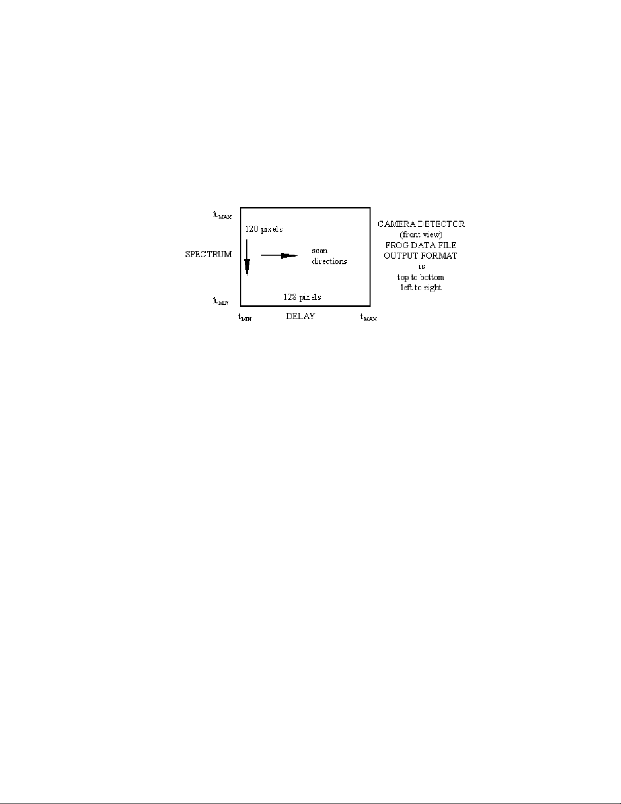
3.1.16.2 FROG Data Orientation
The FROG software has the ability to flip axial assignments and directions. There is, however, a
legacy defined orientation that we use as a basis for defining our axial representations. This is
also the FROG default condition.
Looking into the front of the camera, the upper left corner defines a starting point for the vertical
Spectrum axis and then the horizontal Delay axis. (See figure below).
Figure 12
In the vertical/Spectrum direction, the top represents a maximum wavelength (lowest
frequency), moving down to a minimum wavelength (highest frequency).
In the horizontal/Delay direction, the left represents a minimum time delay moving right to a
maximum time delay.
If you align your axes differently than shown, you can make the necessary adjustments by
altering the Delay and Wavelength settings in the dialog box and in the Exp. Data tab section
of the FROG Algorithm Calibration dialog box.
Note: The LBA-PC always builds the .frg data file in the format depicted above, listing the columns top to bottom
then stepping from left to right.
Reference the FROG on-line Help for details on the FROG data file format.
3.1.16.3 FROG Data Collection Tips
Most of the LBA-PC data collection features are not required when collecting FROG data. Thus,
the Results child window can be minimized, which will speed up data collection. The following
list contains some Do’s and Don’ts for reducing errors when collecting FROG data:
• DO use Ultracal! just prior to starting a data collection cycle.
• DON’T enable Lens in the Camera dialog box.
• DO save your configuration when the camera is aligned with your spectrometer.
• DON’T drive the camera into saturation.
Operator’s Manual LBA-PC
Doc. No. 10654-001, Rev 4.10
47
Page 48

• DO consider Frame Summing if the FROG pulses are too weak to yield sufficient
amplitude.
• DON’T use the pan and zoom features or you will mess up the scaling parameters. You
can minimize the Pan/Zoom child window to reduce temptation.
• DO consider Frame Averaging if the FROG pulses are noisy.
• DON’T enable Convolution.
• DO use the Video Trigger method if pulse amplitude is high enough.
• DON’T use apertures.
Operator’s Manual LBA-PC
48
Page 49

3.2 Options... Drop Down Menu Selections
3.2.1 Hide/Show; Capture, Display, Aperture Toolbar
The above three toolbars can be selectively displayed or hidden based upon operator preference.
Check the action that applies.
The Capture and Display toolbars can be user defined to match the operators needs.
The Aperture toolbar is predefined and can not be altered by the operator.
3.2.2 Aperture... display and define apertures
The LBA-PC can display three types of apertures in four different shapes. The three types of
apertures are:
• Drawn: You can manually draw a WHITE aperture for the purpose of isolating beam
analysis to the pixel data contained within the aperture. This feature allows you to eliminate
the effects of noise or stray energy in regions outside of the beam under test.
• Displayed: The BLACK displayed aperture is not really an aperture. Rather it is an
overlaid graphical representation of the computed shape and size of the beam
width/diameter results. This BLACK aperture provides a way for the user to visually see the
beam width, and observe how it changes.
• Auto: This feature automates the task of drawing an optimally sized and placed aperture
around the beam profile being measured. This aperture is displayed in YELLOW. It
performs the same function as the Drawn aperture, except that it will continuously resize
itself to changing beam conditions.
All three of the above apertures can be enabled and visible at the same time on a 2D display. In the
3D display mode no apertures are ever displayed, however the Drawn and Auto apertures can be
operating as described above. If you’ve enabled the apertures while in the 3D display mode, be sure
to check their setup in the 2D display mode.
The Drawn and Auto apertures, when operating at the same time, function in the following manner:
• First, the Drawn aperture isolates the energy for analysis.
• Second, an Auto aperture is computed and drawn around the beam energy.
• Third, the reported beam widths/diameter is computed based upon the energy contained
exclusively within the Auto aperture.
3.2.2.1 Aperture Shapes
Drawn and Displayed apertures can be rendered in four shapes.
• Circle
• Square
• Ellipse
• Rectangle
Auto apertures are always rendered as an Ellipse.
Operator’s Manual LBA-PC
Doc. No. 10654-001, Rev 4.10
49
Page 50

3.2.2.2 How to create a Drawn Aperture
You can create a Drawn aperture by using the Aperture dialog box, the Aperture toolbar, or by
dragging and dropping the aperture in the 2D display window.
Note: Before you can use the drag and drop method you must first select a Drawn aperture shape using either of
the first two methods.
The Aperture dialog box, and the Aperture toolbar offer the same choices for creating a
Drawn aperture. The entries that define a Drawn aperture are listed vertically within the
recessed panel of the dialog box. These same entries are arranged horizontally on the aperture
toolbar. You can make the same changes from either location. The following discussion will
reference the dialog box, but applies equally to the toolbar.
Choose an aperture Shape. Enter the aperture’s Center location in X and Y coordinate values.
Note: You can modify any edit text control item by double-clicking inside the item and typing the new value.
Figure 13
• If the aperture is an ellipse or rectangle, enter the Size of the Major and Minor
axes, followed by the Rotation angle of the Major axis in degrees.
• If the aperture is a circle or square, enter the Diameter (not shown above).
3.2.2.3 Drag and Drop Apertures
Once you have enabled a Drawn aperture from either the dialog box or toolbar, you can move,
resize, and (in the case of an ellipse or rectangle) rotate it.
Operator’s Manual LBA-PC
50
Page 51
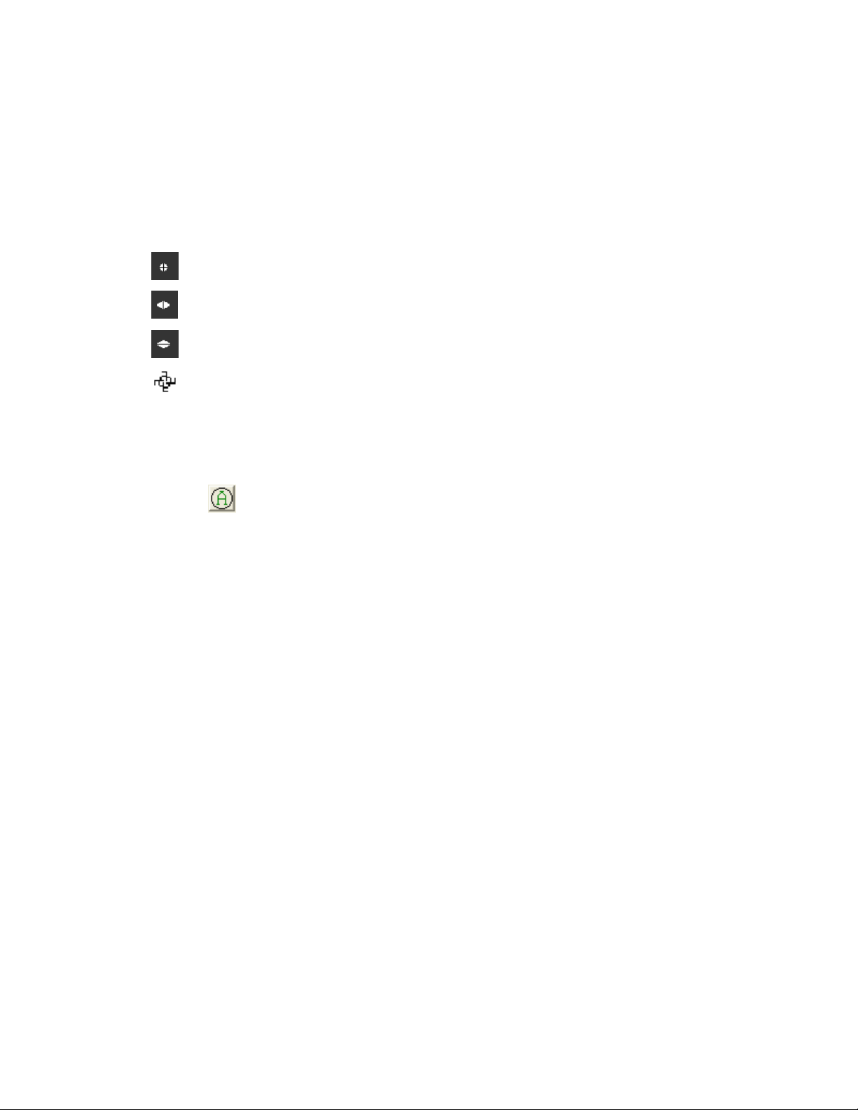
Move the arrow cursor over the display window and press and hold down the RIGHT mouse
button. This will reveal the Drag, Drop and Rotate hot spots of the Drawn aperture.
Move the arrow cursor onto one of these hot spots, release the RIGHT mouse button and press
and hold down the LEFT button. The cursor will change shape indicating the selected Drag and
Drop function.
Now drag the mouse to see what happens to the aperture.
The four cursor styles perform the following operations:
Moves the aperture center.
Size the aperture right or left.
Size the aperture up or down.
Rotate an elliptical or rectangular aperture.
3.2.2.4 Using Auto Apertures
To enable the Auto aperture feature, click on the Use Auto Aperture box, or click on the Auto
aperture button on the Aperture toolbar.
Note: Auto apertures are drawn in YELLOW, are always ellipses, and are only visible on 2D displays. Auto
apertures will be drawn on the X and Y axes of the beam if Elliptical is OFF, and on the Major and Minor axes of
the beam if Elliptical is ON.
You should always enable Auto apertures whenever performing second moment D 4-Sigma
beam width measurements.
If your beam is small, relative to the acquisition window size, you should either use a Drawn
aperture of 2x to 2.5x the beam width, or enable Auto aperturing to perform this task for you.
Auto apertures will help improve beam measurement accuracy on almost any beam shape.
Auto apertures may not improve accuracy, or operate well, if you have a lot of stray energy
adjacent to the beam profile. In this case you should rely more on a well placed Drawn
aperture, and avoid using the D 4-sigma beam width method.
3.2.2.5 Display Beam Width
If you want to see your beam widths/diameter graphically overlaid on the laser beam profile,
choose the shape that most correctly matches your beam.
These choices are also available from the Aperture toolbar.
The displayed beam widths will appear as a BLACK aperture in a 2D beam display window. This
aperture will not appear in 3D displays.
If your beam is an off axis ellipse or rectangle be sure to turn on Elliptical in the Options...
Computations... dialog box. Otherwise all drawn beam widths will be computed and displayed
on the X and Y axes.
Operator’s Manual LBA-PC
Doc. No. 10654-001, Rev 4.10
51
Page 52

3.2.3 Camera... selection and display resolution
The Camera dialog box is where you make the following selections:
• Identify current Camera type, or Create a New Camera type.
• Select the maximum image Resolution.
• Select how large the Frame Buffer will be.
• Select the Sync Source of your camera.
• Modify the Pixel Scale if needed.
• Apply Gamma correction if needed.
• Choose the Lens mode if your camera is so equipped.
3.2.3.1 Camera type selection.
Find your camera...
Camera types are saved in <camera>.cam files. Camera files contain setup information that will
allow the LBA-PC to operate correctly with the specified camera. Included with the LBA-PC
installation is a group of common <~camera>.cam type files. These files include most cameras
that will be used with the LBA, and apply to camera operation without a lens, i.e. the camera’s
detector alone determines the pixel scale. These files are write protected so that you will not be
able to accidentally delete or modify them. To permit easy identification, these write protected
camera files will have a ~ (tilde) symbol included as part of their file name.
Click on the Camera type drop down arrow.
Select your camera type from the list.
If your camera type does not appear:
• Check that your camera path is pointing to the location where the .cam files are stored.
Click on CAM Path... and select the path as required.
• Create a new Camera type.
• Contact Spiricon’s Service Dept. for assistance.
3.2.3.2 Creating a new Camera Type
Do you really need a new camera type?
One common reason that you may need to create a new camera type would be if you use a
camera with a lens that changes the effective pixel scale. In this case it is best to begin by
selecting the supplied common camera type that matches your camera. For example, you might
be using a Pulnix TM-745 style camera fitted with a special lens. Start out by selecting the
~Pulnix_TM-745.cam type and clicking OK. This will cause the LBA to load in all the basic
setup information needed for this camera.
Now return to the Camera dialog box and do the following:
• Double-click inside the Pixel Scale, V edit text control.
Operator’s Manual LBA-PC
52
Page 53

• Type in the new camera pixel scale value.
• Verify that the Pixel Units are set correctly, change as required.
• Double-click inside the Camera type edit text control.
• Type in a new 8 character file name. The .cam extension will automatically be added if
you fail to include it.
• Click on Save CAM...
• If the file path and name specified is correct, click OK.
• You will return to the Camera dialog box. Click OK.
Your new camera is now active, and saved as a <camera>.cam type file.
Note: You may now also want to perform a Save Config... operation, so that when you restart the LBA-PC
application, this new camera setup will automatically be restored. Otherwise, you must return to the Camera
dialog box and select this camera type each time you restart the LBA application.
Notice: A Restore Config... operation will occur each time the LBA application is started. Camera type selections
will only occur when you the operator consciously, unconsciously, but not sub-consciously..., make a choice. Which
ever of the above actions occurs last, is the one that is controlling the Camera dialog box settings.
3.2.3.3 Resolution and Frame Size
The Resolution value specifies how finely the incoming video image is to be digitized. This will
also determine the maximum frame size when viewing an un-zoomed image. The Resolution
value is not related to the resolution performance of your camera.
The smaller the Resolution value, the higher the resolution of the display, and the greater the
number of pixels that will be contained in the un-zoomed image. Consequently, each frame will
take more memory in the frame buffer and on disk, and it will take longer to process the frames,
thus the system will run slower.
The Resolution value will control how much memory is allocated for each frame. This figure does
not change dynamically as you zoom in. In other words, if you set the resolution to 1x, a frame
size of 512x480 is reserved in memory for each frame that is digitized. If you then hardware
zoom in twice, to a frame size of 128x120, you will be wasting 93.75% of each reserved frame
buffer locations space, since a 120x128 image is only 1/15th the size of a 512x480 image.
Thus, you should never specify a resolution that is more than what you need to do the job at
hand. Otherwise, you will waste system resources and reduce your overall throughput.
Analog camera image sizes are fixed to resolution values per the following table:
Resolution
value
Full 1x Hor. Size X Vert. Size n.a
1x 512 X 480 16
2x 256 X 240 64
4x 128 X 120 256
8x 64 X 60 512
16x 32 X 30 2048
Max Frame Size... WxH
(un-zoomed)
≅ Number of frames
in 8 Mb of memory
Operator’s Manual LBA-PC
Doc. No. 10654-001, Rev 4.10
53
Page 54

The Full 1x resolution will create an image size equal to the Horizontal Size and Vertical Size
shown in the Camera…, Advanced dialog box. This size is the maximum obtainable from the type
of analog camera selected.
Digital cameras do not follow the above resolution table. For digital cameras both the Full 1x and
1x resolutions produce image sizes equal to the Horizontal Size and Vertical Size shown in the
Camera…, Advanced dialog box. The 2x, 4x,..etc. sizes will reduce the resolution by
approximately ½ in both the horizontal and vertical directions, rounding to the nearest even
values.
3.2.3.4 Frame Buffer Size
The Frame Buffer Size refers to the total amount of memory that is allocated in your system for
the temporary storage of digitized frames of video. There are two ways to set the size of the
frame buffer. You can enter the amount of memory that you want to allocate to this buffer, or
you can specify the number of frames that you want the buffer to contain. We recommend that
you set the number of Frames, rather than the Buffer Size. This will allocate just the optimum
amount of memory for the set Resolution value.
Figure 14
3.2.3.4.1 What is the Frame Buffer?
The Frame Buffer is an allocated block of memory in your PC. It will receive and temporarily
retain frames of digitized video data. The frames in the Frame Buffer are numbered from 1
to N, where N is the maximum number of frames that the allocated amount of memory can
hold. You must always have at least 1 allocated frame in the frame buffer.
The Frame Buffer is loaded in a sequential round robin fashion. Frames of data can be
placed into the frame buffer by:
• Digitizing the video input signal.
• Transferring data from a digital camera.
• Loading in data from disk files.
• Post processing data already in the frame buffer.
• Post processing data coming from a disk file.
In the far lower right hand corner of the Main Screen display is a Frame edit and spin control
. The number showing in the edit control is the number of the frame
currently displayed. You can edit this number by double-clicking and typing in a new value,
or you can use the spin control to increment or decrement to the frame desired.
We recommend that you set the frame buffer to hold as many frames as your Windows
environment has real memory available. This will prevent the LBA-PC application from trying
Operator’s Manual LBA-PC
54
Page 55

to use virtual memory as Frame Buffer space. A little virtual memory assigned to the frame
buffer is not too bad. A lot can make you wonder what kind of alien being has just taken
over your hard drive.
Also, Windows will allocate real memory first, and when it’s gone, begin allocating virtual
memory. For this reason it is a good idea to run the LBA-PC application with no other
application(s) operating in the background. This will free up as much real memory as
possible for Frame Buffer use.
3.2.3.5 Am I using Virtual Memory yet?
How do I know when my Frame Buffer is running over from real into virtual memory? Easy...,
your hard disk drive light will begin to flicker when the real frame buffer capacity is filled, and the
virtual file swapping begins. To avoid this, try reducing the Frame Buffer size until it stops.
Note: Be sure to perform this test with Logging disabled.
3.2.3.6 Sync Source
Many applications will use standard analog output cameras. For analog cameras the Sync
Source must be set to Genlock. The LBA-400/500/7XXPC models can be purchased with an
option that will allow support for both Analog and Digital cameras. Note: the model LBA-300PC
cannot support digital cameras.
Figure 15
If you have purchased the digital camera option with either an LBA-400/500/7XXPC, and are connecting a digital camera, set the Sync Source to Digital.
In Digital mode, the Pixel Bits entry must be set to the number of data bits that are being
input to the LBA. If you purchased an LBA-400PC-D, you can choose 8, 9, or 10 bits per pixel. If
you purchased an LBA-500PC-D, you can choose either 8, 9, 10, 11 or 12 bits per pixel. If you
purchased an LBA-7XXPC-D, you can choose either 8,10,12,14 or 15 bits per pixel.
If your camera’s digital output is in a signed twos compliment data format, select a minus Pixel
Bits value. For example, the Pyrocam I outputs 12 bit signed 2’s compliment digital data. Thus,
the Pixel Bits setting is –12.
If your digital camera has more bits of resolution than can be accommodated by the LBA-PC, you
must connect only the upper most significant bits. Any left over data bits will not be processed
by the LBA-PC.
Note: There may be some jumper traces on the frame grabber card that will need to be cut if you are using a digital
camera that is outputting fewer bits than the default configuration. The default is 10 bits for the LBA-400PC-D and
12 bits for the LBA-500PC-D. The LBA-7XXPC-D models use the software to set the number of bits rather than
jumpers.
Operator’s Manual LBA-PC
Doc. No. 10654-001, Rev 4.10
55
Page 56

3.2.3.7 Pixel Scale, Pixel Units
For analog cameras that use the Genlock sync source, only the V..ertical Pixel Scale is set.
The pixel scale value is derived from your camera’s detector specifications, or is user
programmable to match the characteristics of your optical system. For the camera imager based
scale setting, the value to enter is the minimum line pitch of the camera’s detector.
For Interline and Full Frame transfer type cameras, the line pitch is the vertical element pitch
of the CCD detector. For pseudo-interlaced Frame transfer type cameras the line pitch is ½ the
vertical element pitch. Check your camera specifications to accurately determine the correct
value to enter here. This value is not always as obvious as it may seem.
Figure 16
The H..orizontal Pixel Scale setting is only used with Digital output style cameras. For digital
cameras the data is clocked by the camera’s element rate clock, and its focal plane array
determines the horizontal pixel scale. In this case you must enter a value that is the horizontal
pixel pitch of the camera.
Choose the Pixel Units that applies to your pixel scale value. Camera detector pixel pitch is
specified in micro-meters (µm), and all provided .cam files are specified in µm.
3.2.3.8 Gamma Correction
If your camera employs a solid state CCD or MOS style detector, then your camera’s detector
responds linearly to monochromatic light. For linearly responding cameras the Gamma setting
should be set to 1.
If you are using a vidicon tube style camera, or a phosphor coated imager, then your output
response is less likely to be linear, and you may need to enter a Gamma correction number that
matches the gamma of your camera. Note: Correction is performed on the entered gamma value
so enter the gamma value of the camera response, not the inverse gamma correction factor.
Notice: Many CCD cameras have selectable gamma settings. Be sure to set your CCD camera to a gamma of 1.
Operator’s Manual LBA-PC
56
Page 57

3.2.3.9 Lens
Click on this box if your camera is fitted with a lens. When enabled the 2D image orientation is
adjusted to depict the image as if the observer is standing and viewing the scene from behind
the camera.
When disabled, the 2D image is oriented as if the observer is standing in front of the camera
looking at the surface of the detector.
3.2.3.10 Special Camera Settings
The Special Camera Settings dialog box contains the electronic parameters that define a camera
to the frame grabber board. All of these values are saved inside of a cameras .cam type file.
We are not going to tell you much about these settings because we don’t want you accidentally
changing something important and running amuck. If you want to experiment with a new
camera type, one that is not in our camera selection list, then we recommend that you call our
Service Department and ask for assistance. We’ll be happy to lend a hand.
Notice: If you change a setting here, and then do a Save Config..., the change will be saved with the configuration
file, and be restored when the configuration file is restored.
3.2.4 Capture... define acquisition method and processing
The Capture dialog box is divided into four areas. These four areas each control different aspects of
the image capturing process. Each area will be discussed separately.
Operator’s Manual LBA-PC
Doc. No. 10654-001, Rev 4.10
57
Page 58
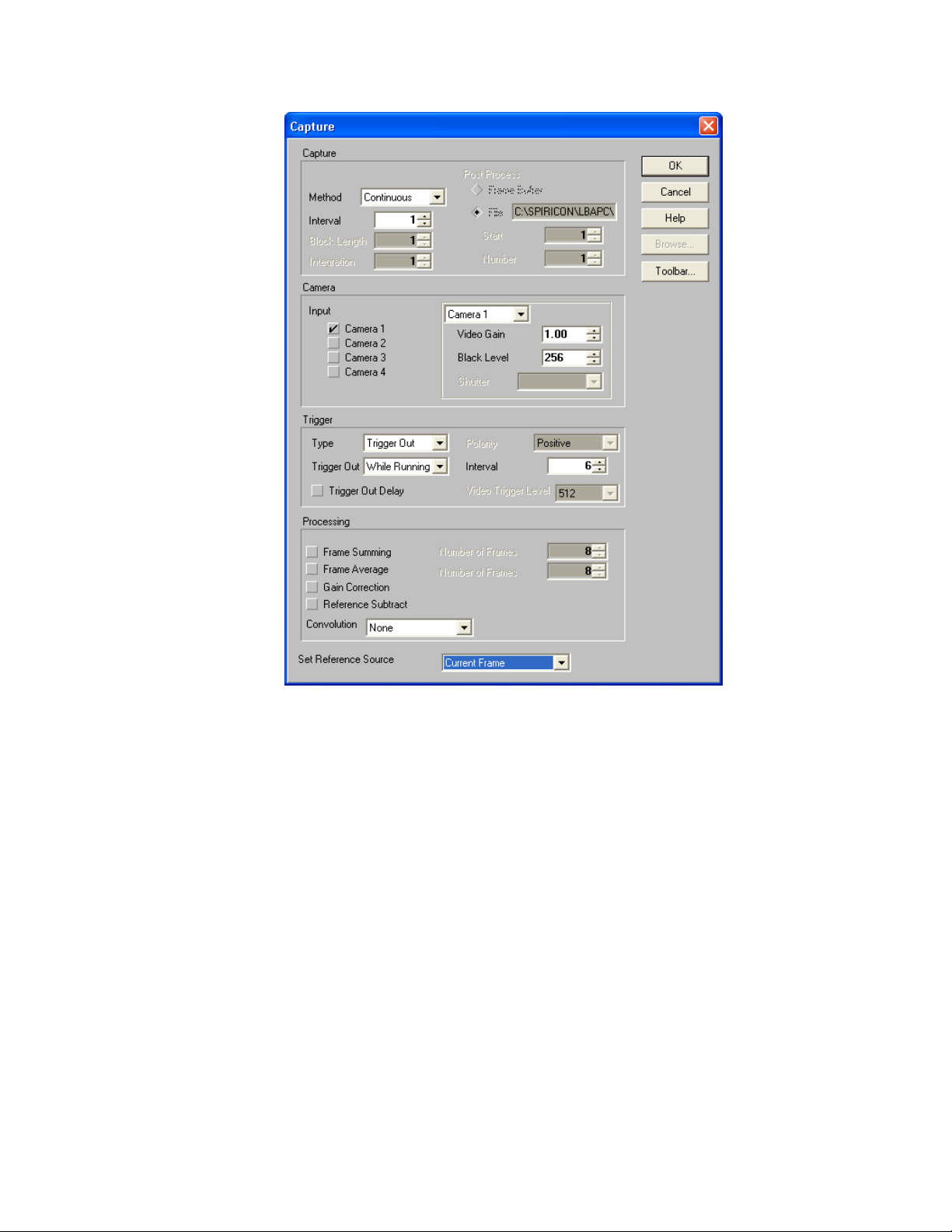
Figure 17
The user can assign certain of these capture control items to the Capture Toolbar. The assigned
items will appear on the toolbar in essentially the same order that they are listed in this dialog box.
The operation of each item from the Toolbar is identical to their operation from this dialog box. For
simplicity, the following examples will refer only to the dialog box entries. Toolbar switch icons will be
included in the titles when they exist.
3.2.4.1 Capture
The Capture panel controls how imaged data is to be acquired and saved into the frame buffer. You must first choose a capture Method, then subsequent selections need to be made. The capture Methods are:
• Continuous: Configures the LBA to continuously acquire new frames of video images
from the frame grabber card as fast as possible, or at a rate determined by the value set
in the Interval edit control. (See 3.2.4.2)
• Single Shot: Choose if you only want to acquire a single frame of video from the frame
grabber card. Each time you click on Start!, the frame grabber will capture one video
Operator’s Manual LBA-PC
58
Page 59
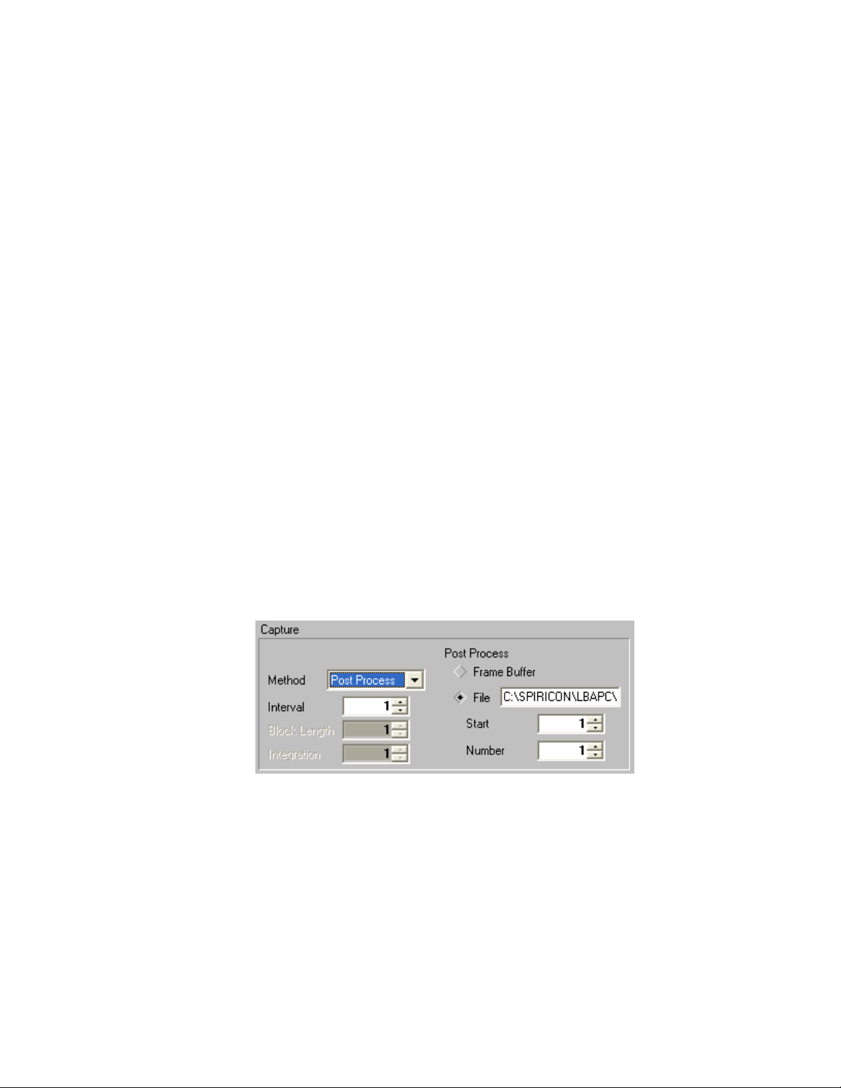
frame, and then Stop!. Successive clicks on Start! will each cause one additional frame
to be acquired. The Interval setting has no effect.
• Block: This method will cause a Block Length specified number of video frames to be
acquired from the frame grabber. What is unique to this method is that the frames will
not be displayed, nor have results computed during the acquisition time. This is so the
frame grabber can capture frames contiguously, with no delays or lost frames owing to
time spent performing results computations. When acquisition of the Block of frames is
completed, the last frame acquired will be displayed and the results computed for that
frame.
Note: If you specify a Block Length larger than the frame buffer capacity, the data will wrap the buffer and
overwrite the earlier frames. The Interval setting is operational.
If you are using Block Mode in combination with Logging or Statistics computations, you
should read Implications of Combining Logging Statistics. . . in Section 3.1.12.
• Live Video: This is a raw video display only method. Video frames will be continuously
acquired based upon the Trigger Type selection and the Interval setting. However,
the data will be totally unprocessed, will not be placed into the frame buffer, and will
yield no computed results. This is best described as the... “is my camera/frame grabber
working?” mode. When you are in the Live Video mode, the Frame indicator will be
forced to a -6, and the Frame Comment will be forced to read Live Frame.
Note: This method only operates in 2D display mode.
Hint: It is best to set the Trigger Type to the CW mode when using Live Video to locate your laser beam on your
camera’s detector.
Figure 18
• Post Process: This method does not collect video frames from the frame grabber, but
rather allows you to run, or rerun, processing of old data that is either already stored in
the frame buffer, or stored in a disk data file. When Post Process is selected, the right
half of the Capture panel becomes activated. Click on the Frame Buffer radio button
to select processing of data already in the frame buffer, or click on File to post process
data from a .lb3/4/5/7 data file. If you have selected File, type in the file name that
you want to source the data from, or click on Browse... to search for the file name. In
either case, you must specify the Start location of either the frame buffer location or the
Operator’s Manual LBA-PC
59
Doc. No. 10654-001, Rev 4.10
Page 60

file record number, and the Number of frames or records to post process. The number
of frames can be 0, or 1 to the number of frames in the frame buffer or file. 0 means all
the frames. The resulting frames will be placed sequentially into the frame buffer,
beginning at the current frame buffer location. Be careful that you do not overwrite
something you intended to save. The post processing toolbar switch
selecting the above file name.
If you are using Post Processing in combination with Logging or Statistics computations, you
should read Implications of Combining Logging, Statistics. . . in Section 3.1.12.
Operating hints:
• When setting up, use the Continuous method with Interval set to 1.
• Always Post Process from a File source.
• You cannot use Post Process to Ultracal old data. It must have been calibrated when it was
captured.
3.2.4.2 Capture Interval
The Interval setting determines the capture rate, up to the fastest rate achievable under the
present setup conditions. The value entered in this edit control specifies how many frames will
occur for each frame captured. A setting of 1, will attempt to capture every frame from the
camera; 2, will capture every second frame; 3 every third; and so on...
Divide this setting into the camera frame rate to compute the rate at which the system will
attempt to digitize frames, i.e., a 3 will cause a 30 Hz frame rate camera to be digitized at 10
frames per second. The ultimate impact of this setting is also determined by the Trigger
Interval setting, see Rate Control in Chapter 5.
is a shortcut to
Note: The fastest achievable frame rate is determined by other factors, including the image size, the speed of your
PC, the type and number of results being computed, the amount of processing being employed.
3.2.4.3 Camera
The Camera panel in the Capture dialog box permits you to:
• Select which camera Input is in use. Note: This choice is only available if you purchased
the four-camera option, see section 3.2.4.3.1 below, otherwise the only available choice
is Camera 1.
• Set the Video Gain level of the signal processing system on the frame grabber card.
Note: If you have the four-camera option, this control will apply only to the currently
selected camera.
• Set the digitizer Black Level threshold. Note: If you have the four-camera option, this
control will apply only to the currently selected camera.
• Program the electronic Shutter setting of your camera, if your camera is equipped with
a remote shutter control feature. Note: If you have the four-camera option, this control
will apply only to the currently selected camera.
Operator’s Manual LBA-PC
60
Page 61

Figure 19
Operating hints:
• Increasing Video Gain also increases video noise. Use Video Gain sparingly, or not at all. Leave
it set to 1 whenever possible.
• The Black Level will be adjusted automatically each time you perform an Ultracal! calibration
cycle. Therefore, it is best that you make no changes to this setting. If you alter the Black Level
after an Ultracal!, the calibration will no longer be valid.
3.2.4.3.1 The Four Camera Option
Some enhancements have been made to the four-camera option with the release of software
version 4.00. These enhancements make it possible to automatically sequence data
collection between multiple cameras (up to four). This sequencing only applies to analog
cameras, and the following operating conditions must be met:
• All cameras must be the same type or model.
• The cameras must be Gen-Locked together.
• If cameras with remotely controlled shutters are used the shutter control circuits
must be paralleled to each camera.
The status of the input video is shown in the video enunciator located at the bottom of the
LBA-PC’s main display window. The number shown in this enunciator indicates which camera
is currently selected. If it shows GREEN then camera sync is present. If it shows RED then
there is either no camera connected, or the connected camera is not operating.
3.2.4.3.2 How to Specify Video Gain, Black Level, Shutter, and Video Trigger Level
On the right side of the Camera panel you will see a panel containing a Camera# dropdown, Video Gain, Black Level, and Shutter controls. Click on the drop-down to select
which camera is affected, the current settings are displayed, and then make the desired
changes. Note that Video Trigger Level, Trigger section below, can also be set for each
camera.
On the toolbar, changing the Video Gain, Black Level, Shutter, and Video Trigger Level
affects only the current camera listed in the video enunciator located at the bottom of the
main display window.
Operator’s Manual LBA-PC
Doc. No. 10654-001, Rev 4.10
61
Page 62

3.2.4.3.3 Automatic Camera Switching Using the Four Camera Option
With the four-camera option automatic switching between camera inputs is made possible by
checking more than one camera enable at a time. Input data frames are repeatedly cycled
into the frame buffer starting with the lowest numbered camera after clicking Start!
Example: If cameras 1, 3 and 4 are checked; data will be placed into the frame buffer
sequentially from camera 1,3,4,1,3,4…, etc. Clicking Stop! will halt data collection at
whichever camera last input data into the frame buffer.
WARNING: Do not check on a camera unless a camera is actually connected to the indicated camera input. An
enabled input without a camera will cause data collection to stall when the nonexistent camera is selected.
.
3.2.4.3.4 Ultracal Operation with the Four Camera Option
If more than one camera is checked on when the Ultracal! menu item is activated, each of
the enabled cameras will be separately Ultracal’d in rotation. Data collected from each
camera will be individually baseline corrected according to its respective Ultracal reference
frame.
3.2.4.3.5 Auto-Exposure Operation with the Four Camera Option
The Auto-Exposure feature will automatically set the exposure or electronic shutter of certain
compatible types of cameras. If the four-camera option is present the LBA application will
attempt to find a correct shutter setting for each enabled camera. It will apply the correct
shutter setting to each camera during the data collection process.
3.2.4.3.6 Acquisition Rate Effects with the Four Camera Option
The data acquisition rate, when cycling between cameras, will depend upon the number and
types of enabled processing features. Without any processing overhead the camera switch
rate is the frame rate of the camera. This means that if one camera can be input at 30
frames per second, then camera switching will progress at 30 switches per second. If your
system is not capable of sustaining this rate, then the resulting rate will be whatever
maximum rate can be sustained.
When various types of image processing, or complex computations are being performed, the
acquisition rate may slow down. These effects will delay the switching rate accordingly. The
rule affecting the switching rate is that it will take as long to switch to the next camera as it
takes to acquire and process data for the current camera.
Note: Image processing rules apply identically to the data inputs of all enabled cameras. I.e. If frame averaging is
enabled then each camera input will be frame averaged before switching to the next camera. It is not possible to
average inputs from multiple cameras during the data collection process. However this can be done using the Post
Processing feature.
3.2.4.4 Trigger
The Trigger panel in the Capture dialog box allows you to selectively control when an image is to be captured by the LBA. The selected trigger Type will govern which of the other selections you will need to make. The four Type choices are:
• CW: Choose this type if your laser operates in a continuous wave manner, or pulses at a
repetition rate that will appear to your video camera as continuous. In CW mode, none
of the other settings in this panel are applicable.
Operator’s Manual LBA-PC
62
Page 63
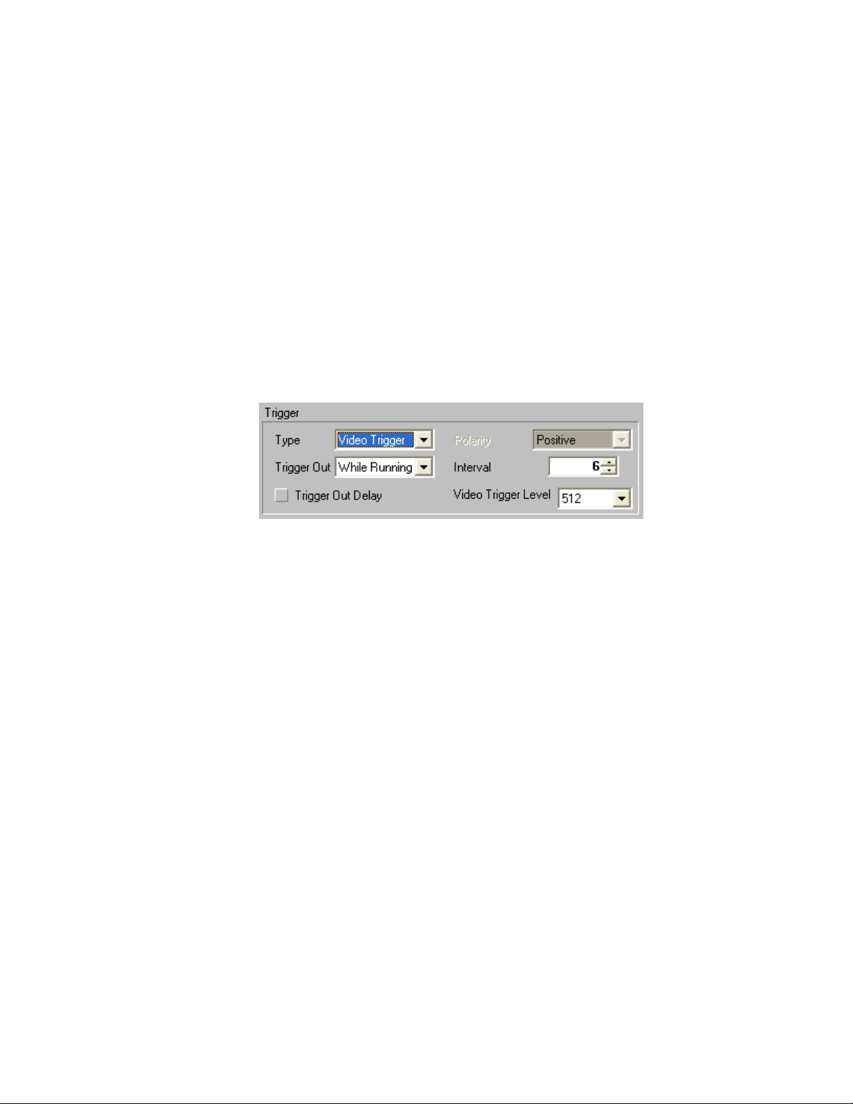
• Trigger Out: If your laser is a pulsed type, and you would like the LBA-PC to provide
an output pulse that will cause the laser to be fired, use this setting. See Trigger Out
and Interval and Trigger Out Delay.
• Video Trigger: With this mode selected, the input from your camera is continuously
monitored, and when a laser pulse is detected, the frame is captured. The pulse
detector has a programmable threshold that is settable in the Video Trigger Level edit
control. The level setting is always in raw digitizer counts. A suggested trigger level
value, that will not detect noise yet remain reasonably sensitive, is the second lowest
level.
• Trigger In: If your laser can provide a compatible trigger input pulse to the LBA, then
you can use that pulse to synchronize the capture of your video frame. In general, this
technique is inferior to the preceding Video Trigger mode. Its only advantage would be
to allow you to capture an event that occurs independently of other things that might be
occurring in the video frame that preclude the use of Video Trigger. See Polarity.
Figure 20
The other settings operate and apply as follows:
• Trigger Out: Applies to Trigger Out and Video Trigger modes. Output pulses from
the LBA-PC can be programmed to output Always, or only when the frame grabber is
sampling video While Running. i.e., beginning when you click Start!, ending when
you click Stop! Note: The output trigger pulse is always positive and its pulse width is
fixed (see Specifications).
• Interval: Applies to Trigger Out and Video Trigger modes. You can program the
rate at which the LBA will produce trigger output pulses. The rate is based upon the
camera frame rate. The value entered in this edit control specifies how many frames will
occur for each trigger pulse generated. A setting of 1, will output a trigger pulse once
for every frame of the camera; 2, will output a pulse on every second frame; 3 every
third; and so on... Divide this setting into the camera frame rate to compute the rate at
which the LBA will output trigger pulses. i.e., a 3 will cause a 30 Hz frame rate camera
to fire a laser at 10 frames per second.
• Trigger Out Delay: Applies to Trigger Out and Video Trigger modes. If this item is
not checked, the trigger output pulse will occur at the same time as the camera’s vertical
sync, i.e. at the start of each video frame. For many CCD cameras, this is not a good
time to receive a laser pulse. If you check this item, the trigger output pulse will be
delayed to a time near the middle of the video frame, or field, if the camera is interlaced.
• Polarity: Applies to the Trigger In mode only. The LBA response to a trigger input is
edge sensitive. You can program the response to the input trigger pulse to be either
Positive, rising edge sensitive, or Negative, falling edge sensitive.
Operator’s Manual LBA-PC
63
Doc. No. 10654-001, Rev 4.10
Page 64

See Chapter 5 for additional information and examples regarding Triggering.
3.2.4.5 Processing
The Processing panel is where you select how to process digitized frames of data. This processing determines how each frame that is stored in the frame buffer will be constructed. This processing occurs prior to the calculating of any numerical results.
Figure 21
The Processing options are applicable to both newly input frames from the frame grabber card,
and to recorded frames that are being Post Processed. Below this panel you can also select
the source for reference frames.
Figure 22
When enabled, the precedence of all processing and post processing operations are as follows
(lowest number occurring first):
1. Ultracal Processing (can not be post processed)
2. Gain Correction
3. Gamma Correction
4. Frame Summing
5. Frame Averaging
6. Reference Subtraction
7. Convolution
Although Ultracal is a processing step it is important to note the following:
• Ultracal processing of newly acquired video is not an option in the dialog above.
• Ultracal processing must be enabled from the main screen Menu bar.
Operator’s Manual LBA-PC
64
Page 65

• Ultracal processing cannot be a part of a post processing operation.
Gamma Correction is also a type of processing. Gamma Correction is controlled from the
Camera dialog box, as it relates to a specific camera’s characteristics. Gamma correction can
be part of a post processing operation.
3.2.4.6 Frame Summing
Click on this item if you want the LBA to sum frames. Specify the Number of Frames that you
want to sum into each frame placed in the frame buffer. Frames are always summed in the
order that they are input. Frame summing can be used to increase the apparent size of low-level
signals. Fixed pattern noise will unfortunately grow linearly with each summed frame, but
temporal noise will increase at approximately the square root of the number of frames summed,
thus the resulting signal to noise ratio will be improved.
3.2.4.7 Frame Average
Check on this item if you want the LBA to average frames. Specify the Number of Frames that
you want to average into each frame placed in the frame buffer. Frames are always averaged in
the order that they are input. Frame averaging will improve the signal to noise ratio by
approximately the square root of the number of frames averaged.
Note: If the frame that you are averaging has poor pointing stability, then the reliability of the computed results of
an averaged frame may not be very good.
3.2.4.8 Gain Correction
Check on this item if you want to apply Gain Correction. You must have Generated or Loaded a gain correction table, before you can apply gain correction processing to newly acquired or post processed frames of data. See 3.1.8 Generate Gain, for further details.
3.2.4.9 Reference Subtraction
Check on this item if you want to subtract the reference frame from newly acquired or post
processed frames of data. The reference frame is location 0 (zero) in the frame buffer. This
location is always reserved for the reference frame. The content of frame 0 will be subtracted
from the results of all other processing operations. Associated with creating and saving a
reference frame is the Set Reference Source edit control (shown above), and the Set
Reference action item in the Files menu, and the set reference toolbar button.
Reference for further details.
The Set Reference Source edit control allows you to select what type of data will be loaded
into the reference frame.
See Set
Using this feature with the four-camera option will cause the reference frame to be subtracted
from the input of each camera. It does not discriminate between camera selections.
Operator’s Manual LBA-PC
Doc. No. 10654-001, Rev 4.10
65
Page 66

Note: This edit control is repeated in the Beam Display dialog box and is available in the Display Toolbar.
• If the Set Reference Source item is set to Current Frame, the data in the currently
viewed frame will be copied to the Reference frame.
• If the Set Reference Source is set to Last Gauss, and the Gauss Fit item in the
Computations... dialog box is checked, then the beam profile resulting from a
computed Gaussian fit to the currently viewed frame will be copied to the Reference
frame.
• If the Set Reference Source is set to Auto Gauss, and the Gauss Fit item in the
Computations dialog box is checked, then the beam profile resulting from a computed
Gaussian fit to newly acquired frames will be automatically copied to the Reference
frame. In this mode, setting a reference frame manually does not make any sense
because the next frame brought into view will automatically update the contents of the
reference frame.
Note: In the last two examples, if the Gauss Fit item is not Checked, then no fit is computed and thus no data will
be copied to the Reference frame.
3.2.4.10 Convolution
The term Convolution indicates a type of two-dimensional spatial filtering that can be applied to a digitized image. We will not attempt to use this term in any restricted construct. Rather we will apply it generally to a variety of area process transformations. At the time of this release we are providing just a few convolution algorithms, these primarily aimed at simple low-pass spatial filtering. We expect this list to grow in time, and welcome suggestions from our users for additional implementations.
Click on this edit control to see a list of Convolution algorithms. Entries in this list that begin
LPF #, indicate a Low-Pass filter. This is the most commonly used algorithm for simple image
smoothing operations. The numbers following define the size of the convolution kernel in pixels.
For example, 3x3 indicates a 9 pixel kernel 3 pixels by 3 pixels. Other common sizes are 5x5 and
7x7.
We recommend that you experiment with these selections until you find a process that meets
your specific needs.
See Convolution in Section 6.27 for more details regarding how these algorithms are applied.
3.2.5 Capture Toolbar... design the toolbar contents
You can select which functions you want to appear on the Capture Toolbar by checking the desired
item. The functions will appear on the toolbar in the same order that they are listed in this dialog
box. The first four panels; Capture, Camera, Trigger, and Processing, are analogous to the items
listed in the Capture dialog box.
The panel labeled Other offers you the following two tools that are associated with File menu items,
and a third item that is not available anywhere else.
Operator’s Manual LBA-PC
66
Page 67

3.2.5.1 Logging
This switch will launch you into the Data & Results Logging dialog box.
3.2.5.2 Print
This switch will cause the selected print options to be printed on your configured printer. You
will not get a chance to reconfigure your printer or print setup item when you click this tool, so
be sure that you have set your options up in File, Print Setup... before you click here.
3.2.5.3 Write Protect
This tool can be used to write protect any frame in the frame buffer. Before clicking on this tool,
be sure that the frame number that you want to write protect is indicated in the frame counter.
The frame counter is located in the lower right corner of the main window.
When a frame has been write protected, its location in the frame buffer can not be overwritten.
When new data is flowing into the frame buffer, write protected locations will be skipped.
To un-write-protect a location, bring the frame number up again and note that the write protect
button is still in the depressed position; click the tool a second time. This tool’s button will show
in the un-depressed state to indicate that the frame is no longer write-protected. Therefore, the
only way to determine which frames are write-protected is to cycle through the frames and
simultaneously view the up/down state of the write-protect button.
Caution: If you change the frame buffer resolution, all write protected frames and their contents will be deleted.
3.2.6 Computation... Energy calibration select results items
The Computations dialog box is where you select the types of numerical results that you want to
have calculated and displayed. You can also calibrate the beam energy here.
Italic
Note: The term energy, shown in
3.2.6.1 Energy of Beam
The Energy of Beam edit control item lets you calibrate the LBA to the
You must measure the
energy
entered must be the total
beam must be completely contained inside the current Hardware Zoom/Pan window, and an
Ultracal! operation should be performed prior to collecting the frame used for
calibration.
value here. Next select the appropriate units in the
, will be used to represent both Energy and Power.
energy
energy
of your beam using an external measuring device, then enter the
Energy
energy
of the frame currently displayed. For accurate results, the
Units item. The value
of your laser.
energy
Operator’s Manual LBA-PC
Doc. No. 10654-001, Rev 4.10
67
Page 68

Figure 23
If you enter an Energy of Beam value of 0 (zero) the
Total (
digitizer units. Processed digitizer units are called counts, and are dimensionless. In this case,
no units will be displayed in the results window.
Any non-zero entry will cause the displayed results to be reported in the units selected. Fluence
results will also rely upon the Pixel Units entry to complete the energy density definition. A
Pixel Unit selection of PX stands for pixel spatial units. The PX unit is dimensionless.
When the Scale Units are set to µm, mm, or cm, the
energy
energy
energy
/cm². When the scale units are set to PX or m, the density results are displayed as
/PX², or
), Peak (fluence), Min, Gauss Height, etc., will be computed in processed
energy
/m² respectively.
3.2.6.2 Energy Calibration Procedure
After you have set up the LBA-PC and are ready to acquire data, the
involves the following three operation:
1. Execute an Ultracal! operation.
2. Acquire a calibration frame on the 2D display and a matching
external power/energy meter.
3. Enter the
energy
and select the units in the Computations dialog box.
energy
energy
related results items, such as,
density results are computed as
energy
calibration procedure
energy
measurement on an
3.2.6.3 Quantitative display, on/off
Check the Quantitative box if you want to have the quantitative results item appear in the results
window. Checking this box only controls the display of these results. Even if not checked, these
results will be computed. The only way to turn off all computational activity is to minimize the
Results display window. The displayed quantitative results consist of the following:
• Total
• % in Aperture
• Peak fluence
• Min
• Peak Loc..ation, in X and Y
• Centroid location, in X and Y
• Beam Width, in both X and Y or Major and Minor axes
• Beam Diameter
Operator’s Manual LBA-PC
energy
68
Page 69

For a detailed discussion of the above items see Chapter 4, Results Display, and Chapter 6,
Computations.
3.2.6.4 Beam Width Method
The Beam Width Method edit selection will determine the technique used to compute the
beam width results. The first two methods (4 Sigma and 90/10 Knife Edge) are computed
based upon industry standard definitions. The remaining three choices are user definable, so use
care in setting up and restoring their related options. See Beam Widths and Diameters in Chapter
6 for a technical discussion of the methods described here.
Notice: Beam Width measurements should never be made without Ultracal! processing. Failure to perform an
Ultracal! operation will most certainly lead to inaccurate beam width results.
Note: The Diameter results are always computed as the mean of the two Beam Width results.
The five Beam Width Methods are:
• 4 Sigma
• 90/10 Knife Edge
• Knife Edge (user definable)
• Percent of Energy (user definable)
• Percent of Peak (user definable)
Figure 24
3.2.6.4.1 D4 Sigma
The 4 Sigma, or second moment method, will directly compute second moment beam
widths in the X and Y beam axial directions, or along the computed orthogonal Major and
Minor axes of the beam if the Elliptical calculations are enabled. The 4 Sigma method
should always be used in conjunction with the LBA’s Auto Aperture feature. The 4 Sigma
method is most sensitive to noise. If your camera or beam noise content is high you might
want to employ Frame Averaging or Statistical analysis to home in on more accurate
results. A big advantage of this method is that it is not influenced by mode content.
Operator’s Manual LBA-PC
Doc. No. 10654-001, Rev 4.10
69
Page 70

3.2.6.4.2 90/10 Knife Edge
This Knife Edge method uses a fixed 90% and 10% of energy as the moving edge Clip% points. The correction Multiplier is fixed at 1.561. These settings will yield highly accurate second moment equivalent beam widths for beams that are predominantly TEM
in mode
00
content, and for many other mixed mode combinations. There are a few modes for which
this method will not be as accurate, as well as Top Hat shaped beams. This method will
compute beam widths in the X and Y beam axial directions, or along the computed
orthogonal Major and Minor axes of the beam if the Elliptical calculations are enabled.
3.2.6.4.3 Knife Edge
If your laser mode content is not suitable for measurement using the previous Knife Edge
method, then you can use this method and program your own Clip and Multiplier factors.
For example if your beam is almost a pure donut shape (TEM
*), use the previous 90 and
01
10 Clip% setting, but change the Multiplier to 1.533. For a circular Top Hat, use a
Multiplier of 1.455. For a square Top Hat use a Multiplier of 1.444. This method will
compute beam widths in the X and Y beam axial directions, or along the computed
orthogonal Major and Minor axes of the beam if the Elliptical calculations are enabled.
Hints: In general, your two Clip level settings should add up to 100%. Avoid using clip levels of <10%, as this
begins to approach the camera’s noise floor, especially if your beam peak energy is less than 20% of camera
saturation.
3.2.6.4.4 Percent of Energy
This method will only use a limited amount of your beams energy to compute beam widths.
In particular, it will only use the data from pixels on the X and Y axes of the beam that pass
nearest to the computed centroid. If you have the Elliptical computations enabled, then the
data used for this calculation will be from those pixels that lie along the Major and Minor
axes. The Percent of Energy method requires that you set a Clip % value that
corresponds to the percent of energy that will be used to define the beam width. For
example, set the clip value to 86.47% if your beam is mostly a Gaussian TEM
mode. The
00
resulting beam widths will then be a 1/e², or second moment equivalent value.
3.2.6.4.5 Percent of Peak
This method will only use a limited amount of your beam’s energy to compute beam widths.
In particular, it will only use the data from pixels on the X and Y axes of the beam that pass
nearest to the computed centroid. If you have the Elliptical computations enabled, then the
data used for this calculation will be from those pixels that lie along the Major and Minor
axes. The Percent of Peak method requires that you set a Clip % value that corresponds
to the percent of your beams peak that will be used to define the beam width. For example,
set the clip value to 13.53% if your beam is mostly a Gaussian TEM
mode. The resulting
00
beam widths will then be a 1/e², or second moment equivalent value.
Hint: This method is most useful to measure the widths of Top Hat beams typically based upon a Full-Width-HalfMax (FWHM) criteria. To achieve this set the Clip% to 50%.
Operator’s Manual LBA-PC
70
Page 71

3.2.6.5 Elliptical
Check on the Elliptical box to cause elliptical calculations to be performed. Having Elliptical results enabled will cause the nature of other calculations to be modified. In particular, Beam Width results will now be computed based upon the orientation of the Major and Minor axes of the beam, instead of the X and Y axes, as will the aligned Gauss Fit and Divergence results. See Elliptical in Chapter 6 for additional details.
3.2.6.6 Gauss Fit
Check on the Gauss Fit box to cause the Gaussian fitter results to be displayed. Gauss Fit computes a best fit of a Gaussian distribution to the data. Two types of fits are available. One is Whole Beam, and the second is X/Y or Major/Minor aligned. The Whole Beam choice computes an X,Y axial aligned fit to all of the data. The aligned choices perform two separate line fits using just the data that passes through the centroid, along the X,Y or Major, Minor axes. See Gauss Fit in Chapter 6 for additional details.
Figure 25
3.2.6.7 Top Hat
Check on the Top Hat box to cause the Top Hat results to be displayed. Top Hat results
include Mean, StdDev, (Std/Mean)%, Min, Max, Top Hat Factor, Effective Area and
Effective Diameter. You must choose one of the three methods that determine how the Top Hat results are computed. These choices and their affects are:
• Data: This method will include all data above the Clip% level. If you are using 4
Sigma, or one of the Knife Edge beam width methods, the Clip% level is forced to
80% of peak.
• Area Aperture: Only available if an Aperture is present. This method will restrict the
calculations to all data inside the Aperture. The clip level is only used to compute
Effective Area and Diameter and has no effect on the other results.
• Line Aperture: Only available if an Aperture is present. This selection causes two
separate Top Hat results to be computed along the orthogonal axes of the Aperture. The
clip level is only used to compute Effective Area and Diameter and has no effect on the
other results.
Notice: If you disable the Aperture, in either the Area or Line Aperture modes, the above setup will
automatically revert to Data.
Operator’s Manual LBA-PC
Doc. No. 10654-001, Rev 4.10
71
Page 72

Hints: Use Drawn apertures and avoid Auto apertures when making Top Hat measurements. Use Percent of
Peak as your beam width method. Typical Percent of Peak Clip% settings are 50%, 80%, and 90%.
Refer to the Top Hat section in Chapter 6 for additional details.
3.2.6.8 Divergence
Two methods are provided for making divergence measurements of your laser beam. The
preferred technique is the Focal Length method. The Focal Length method can produce a
valid result anywhere in the laser beam path and only requires one measurement.
A second technique, referred to as the Far-Field method, is also provided. The Far-Field
method is only valid if you are sampling your laser in the far field. It will give incorrect results if
you are measuring your laser in the near-field. The Far-Field method requires you to make two
sets of beam width measurements a known distance apart.
See Divergence in Chapter 6 for details regarding how these two methods are computed.
3.2.6.8.1 Focal Length Divergence Measurements
The Focal Length method requires you to bring your laser beam to a focus using either a
focusing lens or mirror. You must place your camera detector at the focal point of the
focusing optic. One-half to one-meter focal lengths are typical, as they will keep the focused
spot size large enough to be measured with a CCD camera.
Check the Divergence box and select Focal Length in the drop down edit control. Enter the Focal Length of your optical system in meters. The divergence results will be computed for both the X and Y or the Major and Minor beam widths, depending upon Elliptical being enabled.
Figure 26
The Focal Length method is most appropriate for lasers that exhibit small angular
divergences. For larger divergence angles, like those seen with laser diodes, the Far-Field
method is much more accurate.
Operator’s Manual LBA-PC
72
Page 73
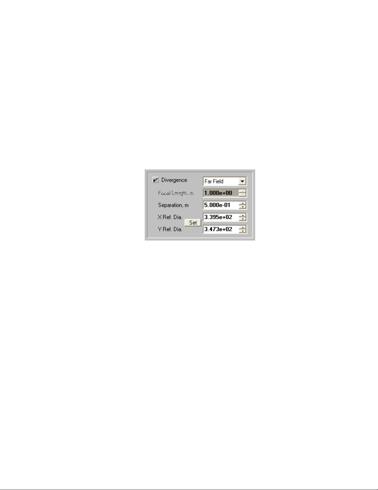
3.2.6.8.2 Far-Field Divergence Measurements
The Far-Field method requires you to measure the beam widths of your laser at two known
locations in the beams far-field. The change in size is used to compute the rate of beam
divergence in mili-radians.
First collect a pair of Reference beam widths. The Reference data should be acquired at
the smaller beam width location. Click Stop!, and note the location of your camera in the
beam path.
Open the Options…Computations dialog box. Check the Divergence box and select Far
Field in the drop down edit control. Click the Set button to transfer the current Reference
beam widths into the provided edit control boxes.
Note: You can manually enter these values from a previous measurement if you know what they are. The Set button
is provided to facilitate making this entry.
Figure 27
Move your camera to the larger beam width sample location, noting the distance traveled by
the camera. The distance traveled is the separation distance between the two sample
locations. Enter this Separation distance in meters. Click OK and then Start! The
divergence results will be computed for both the X and Y axes based upon how the current
beam size has increased from that of the Reference sample.
Notice: It is not recommended that Elliptical be enabled when making this measurement, rather you should rotate
your laser/camera to be X and Y axis aligned. Under certain conditions the rate of divergence could cause the
major and minor axes to swap in the far field region, yielding false results.
3.2.6.9 Histogram
Check this box if you want to view a Histogram of your laser beam’s energy distribution. The Histogram graphic and numerical results will appear in its own window of the LBA’s main display. The size of each bucket in the histogram is user programmable. Bucket size is based upon the integer values produced by the A to D converter. If required, the bucket size will be converted to floating point values to reflect the processing effects of an energy calibration. The buckets are sized up (plus) and down (minus) from zero.
Operator’s Manual LBA-PC
Doc. No. 10654-001, Rev 4.10
73
Page 74
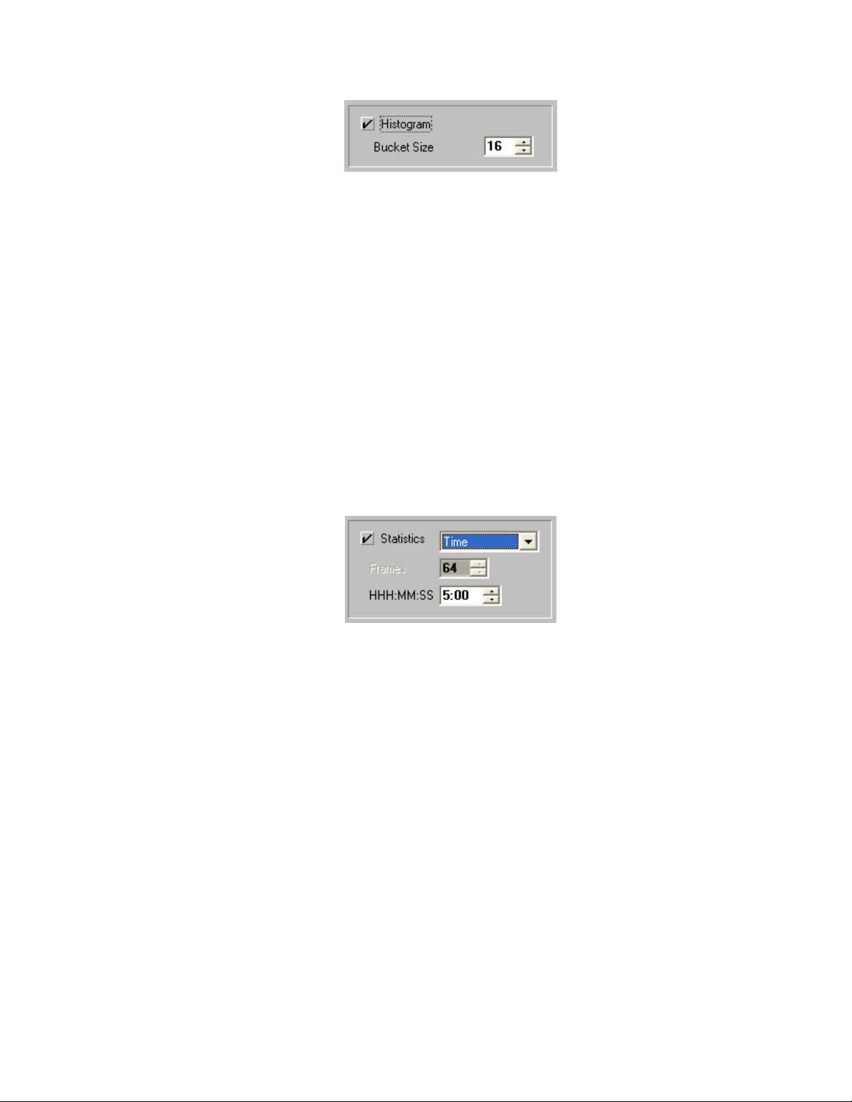
Enter the Bucket Size in the provided edit control. A good value to start with is 16, 64, 256 or
1024, depending upon which model frame grabber you are using; an 8, 10, 16, or 14 bit format
respectively.
Refer to the Histogram section in Chapter 6 for additional details.
3.2.6.10 Statistics
Check this box to enable the addition of Statistical information in the Results window. Statistical
results will be computed for every numerical results item that is appearing in the Results window.
The statistical results provided are: Mean, Standard Deviation, Maximum, and Minimum.
To view the statistics results you must either maximize the Results window, or use the horizontal
scroll bar to bring the values into view.
Figure 28
Figure 29
There are three ways to control how many samples are used to generate the statistical results
calculations. The following choices and their usage is as follows:
1. Continuous: Statistical results will begin to accumulate when you click Start!, and do so
until you click Stop!.
2. Frames: Enter the number of frames of data that you want to accumulate for statistical
purposes. After you click Start! the LBA will run until the number of frames is collected
and then automatically Stop!.
3. Time: Enter the collection duration in Hours:Minutes:Seconds that you want to
accumulate statistical results. After you click Start! the LBA will run until the time is
depleted and then automatically Stop!.
In all of the above, you can click Stop! and click Start! to pause and to resume statistical data
collection. However, in cases 2 and 3 above, when you restart, it does not resume the cycle
Operator’s Manual LBA-PC
74
Page 75

from the point of interruption. Rather the cycle resets to the duration values set in the dialog
box, but does not clear the prior accumulated stats.
If you click on Start! after the frame count or timer has run out, the collection process will
continue to add more data to the results until the cycle completes a second time.
To reset statistical data operations you must turn Statistics off, click OK, and then turn
Statistics back on. Or right click in the Results window and click on the Results Statistics
item.
When collecting Frames or Time limited Statistics, the Rate display will indicate the number of
frames to go,
or the time remaining
If you are using Statistics computations in combination with Logging, Block Capture, or Post
Processing, you should read Implications of Combining Logging, Statistics. . . in Section 3.1.12.
Refer to the Statistics section in Chapter 6 for additional information
3.2.7 Beam Display... define the beam display
The LBA-PC has a number of display options. The operation of these options can vary depending
upon whether the 2D or 3D display mode is in effect. Options in the Beam Display dialog box that
are shared by both 2D and 3D modes will be discussed first. Separate sections are provided for those
options that are exclusive to either the 2D or 3D panels.
The user can assign certain of these display control items to the Display Toolbar. The assigned
items will appear on the toolbar in essentially the same order that they are listed in this dialog box.
The operation of each item from the Toolbar is identical to their operation from this dialog box. For
simplicity, the following examples will refer only to the dialog box entries. Toolbar switch icons will be
included in the titles when they exist.
• Beam View
• Cursors
• Cursor Orientation
• Origin Location
• Beam Colors
• Z Axis Scale
• Beam Display
• Set Reference Source
• Display Thresholds
• Color Bar
• Copy Image to Clipboard
• Copy Image to Wallpaper
Operator’s Manual LBA-PC
Doc. No. 10654-001, Rev 4.10
75
Page 76

3.2.7.1 Beam View
Inside the Beam Display… dialog, click either the 2D or 3D radio button for the display mode
that you want to view your beam in. You may also toggle beam display with the 2D/3D button
on the toolbar.
Note: In general 3D displays will run slower than 2D owing to the amount of computations involved with
generating the wire frame.
3.2.7.2 Cursors
You may choose to place cursors onto either a 2D or 3D display. The cursors will appear as two
black and white dashed lines in a 2D display and as solid white lines in a 3D display. Cursor
options include:
• Off: No Cursors will be displayed.
• Manual: Cursors will be displayed, and the operator manually determines their location.
• Centroid: Cursors will be displayed, but their location is automatically drawn to pass
through the computed centroid of the beam.
Note: This operation will revert to Manual if the results window is minimized.
• Peak: Cursors will be displayed, but their location is automatically drawn to pass
through the peak energy location of the beam.
Note: This operation will revert to Manual if the results window is minimized.
There are two ways to move and position the Cursors in the 2D display mode, and only one way
to move them in the 3D mode.
At the bottom of the main display window are two spin controls, one labeled X: and one Y:.
These controls indicate the location of the Cursor’s intersection. The Value: displays the
at the Cursor’s intersect point. You can edit these controls to redraw the cursors to a new
location.
Note: The above method is the only way to move the cursors in the 3D display mode.
The second way to move the Cursors is to use the mouse to drag and drop them. Move the
mouse pointer to the intersection of the Cursors. When the pointer changes to the cursor drag
symbol,
Release the mouse button to drop the Cursors.
The Cursors can also used to fix the Manual Origin Location. (See 3.2.7.4)
press and hold down the left mouse button and drag the Cursors to a new location.
3.2.7.3 Cursor Orientation
energy
The Cursors can be orientated to align with either the X/Y axial directions, or with the computed
Major/Minor axial directions.
Operator’s Manual LBA-PC
76
Page 77
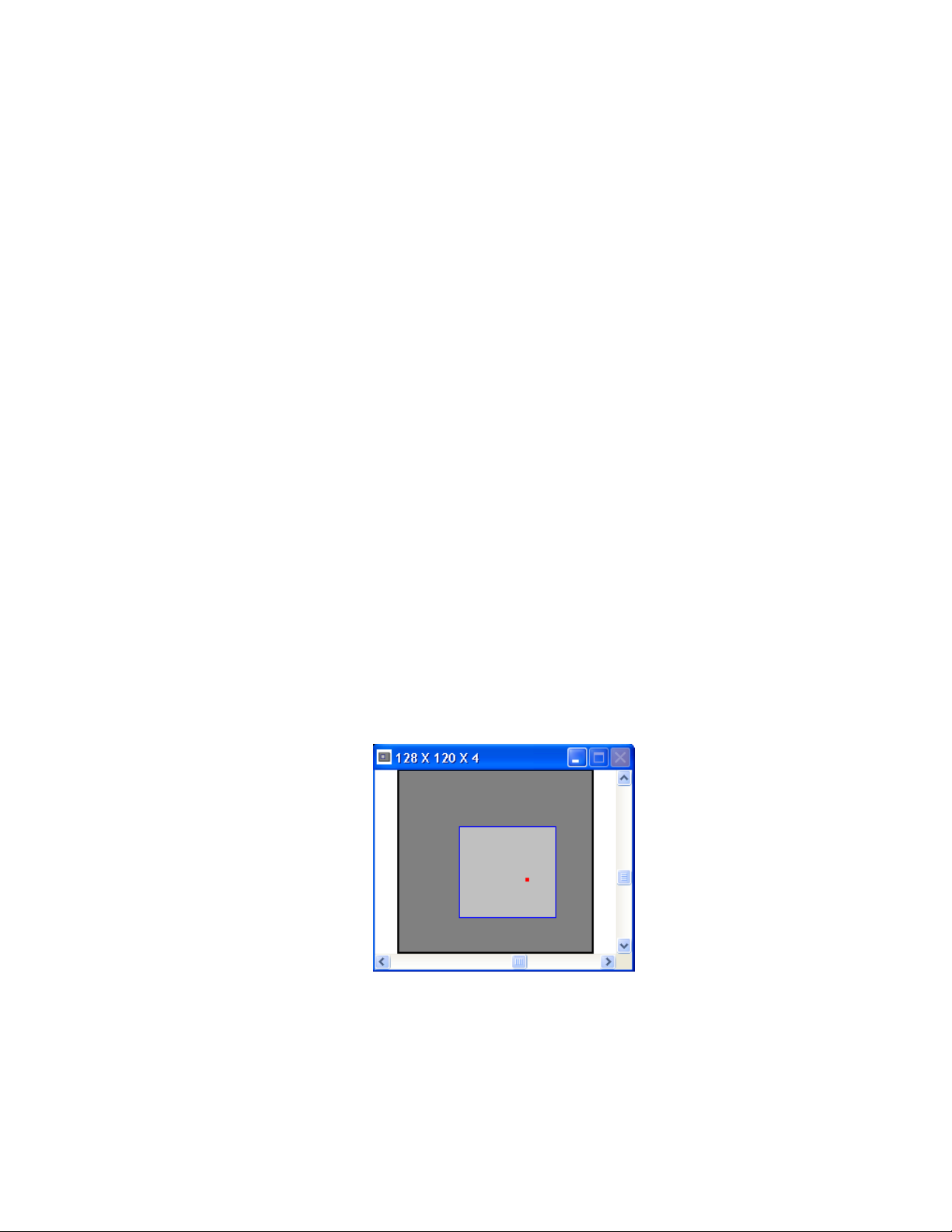
Note: You must have the Elliptical computations turned on to permit the Major/Minor orientations to operate
correctly, otherwise it will revert to the X/Y operating mode.
3.2.7.4 Origin Location
The beam display window will always have an X/Y origin from which all other positional data will
be referenced. A red dot visible in the Pan/Zoom window will indicate where the Origin location
is set. The operator can choose one of four defaults, or manually locate the origin. The four
defaults are:
• Detector UL: The origin will be the upper left-hand corner of the camera detector as
referenced in the display Pan/Zoom window.
• Detector LL: The origin will be the lower left-hand corner of the camera detector as
referenced in the display Pan/Zoom window.
• Window UL: The origin will be the upper left-hand corner of the Pan Window as
referenced in the display Pan/Zoom window.
• Window LL: The origin will be the lower left-hand corner of the Pan Window as
referenced in the display Pan/Zoom window.
Note: In the first two selections, the Origin is absolutely referenced to the camera detector, and thus the Pan
window moves over the coordinate system just as the cursors do. In the last two selections the Origin is located
only with respect to the Pan window, thus the Origin moves relative to the detector as the Pan window is moved.
Manual origin locations are always absolutely referenced to the camera detector, see note
above. You must be in 2D display mode and have the Cursors enabled to manually place the
origin. Move the Cursors to the location where you want the Origin be placed, then double
click the right mouse button. Observe that the X: and Y: cursor locations now show zeros.
Also observe that the Pan/Zoom window’s red dot is in the approximate location inside the Pan
window where you just placed the Origin.
Figure 30
Note: If the Origin is set to Manual, and the Crosshair is set to Origin, then you can move the Origin by dragging
and dropping the Crosshair.
Operator’s Manual LBA-PC
Doc. No. 10654-001, Rev 4.10
77
Page 78

3.2.7.5 Beam Colors
Your choice of beam display colors depends upon which display mode you have selected. There
are 3 choices available in both 2D and 3D modes, plus 2 additional choices in 3D mode. They
are:
• Color Bands: 16 colors plus white to indicate intensities at, or near, A/D converter
saturation. Available in both 2D and 3D.
• Color Continuous: 128 colors plus white to indicate intensities at, or near, A/D
converter saturation. Available in both 2D and 3D.
• Gray Scale: 128 shades of gray plus red to indicate intensities at, or near, A/D
converter saturation. Available in both 2D and 3D.
• Green: Available only in 3D mode, a monochrome shade of green that can be used with
laser goggles that do not filter the green wavelengths. White is used to indicate
intensities at, or near, A/D converter saturation.
• Yellow: Available only in 3D mode, a monochrome shade of yellow that can be used
with laser goggles that do not filter the yellow wavelengths. White is used to indicate
intensities at, or near, A/D converter saturation.
Note: In the above selections, data that is representing negative energy values will be displayed in dark gray,
except in the case of the gray scale, dark blue.
• User Palette: This selection allows the user to select a color palette that they have
custom designed. When selected a Palette button
Toolbar. When you click on this button you will be allowed to select one of your custom
palette files for both 2D and 3D displays. See section 3.2.10 about how to create a
custom palette.
These basic color schemes can be augmented by some other display choices. In particular,
choosing Z Axis Scaling greater than x1, enabling 3D Contour displays, and Beam Display
selections that involve more than one beam at a time will modify how your beam will be
displayed.
3.2.7.6 Z Axis Scale
You can expand the intensity or Z Axis Scale in both 2D and 3D display modes. An expanded Z
axis will allow you to view a narrower range of intensities in more detail. The Z axis scaling will
yield slightly different imaging results depending upon which Beam Colors you have selected. To
activate Z Axis Scaling, select a magnification factor greater than x1. A good value to practice
when using this feature is a conservative x2. When Z axis scaling is activated, a vertical scroll
bar will appear along the right edge of the beam display window. You can use this scroll bar to
slide the expanded viewing range up or down the full Z axis scale.
In 3D mode, it is easy to see where the expanded display region boundaries end and the
outside region begins. To assist you in the 2D display mode, a pair of dashed lines will indicate
the magnified range in the Cursor Profiles. Of course, to see these indicators you must have
the Cursor Profiles turned on and the Cursors passing through the beam profile.
will appear in the Display
Hint: Use Z Axis Scaling with: Beam Color set to Color Continuous, 2D Cursor Profiles turned on, and Cursors
set to Centroid.
Operator’s Manual LBA-PC
78
Page 79

Another Hint: A good time to use Z Axis Scaling is when you need to view the low energy down in the wings of
your laser beam. Kick the scaling up to x8, leave the scale scroll bar at the bottom of the slider, and maybe add in a
little video gain and some frame averaging to quiet the noise. You’ll be amazed at what you can see!
3.2.7.7 Beam Display
You can change how your beam is displayed without actually changing how it is processed nor
how it is stored in the frame buffer. With these choices you can visually compare your Current
selected Beam Display to a beam profile stored in the Reference frame buffer. Or compare it
to your beam with the reference added or subtracted from it. Or just display your current beam
added to or subtracted by the reference beam.
The choices here seem obvious, however the impact on your display may be a bit disconcerting
when first viewed, so some explanation is in order.
First, the definition of Current means the frame buffer location indicated in the frame counter at
the bottom of the main display window. In other words, the frame you currently have decided to
view. If you are running, then the current frame will be cycling.
The Reference frame is whatever you last saved into the reference frame buffer, location 0
(zero).
For 99% of the majority of users the Beam Display will be set to Current Alone, and rarely be changed.
For those other 1%, and you know who you are, read on...
3.2.7.7.1 Current and Reference:
2D You must have both Cursors and Cursor Profiles enabled for this feature to operate.
The Current beam alone will appear in the display. A second profile, drawn in Lt. Gray will
also appear in the display. This profile is a projection of the Reference beam. All projections
are made from the Cursor positions.
3D The Current beam will be displayed in Red. The Reference will be displayed in Blue. If
cursors are enabled they will follow the contour of the Current beam.
3.2.7.7.2 Current and Current - Reference:
2D You must have both Cursors and Cursor Profiles enabled for this feature to operate.
The Current beam alone will appear in the display. A second profile, drawn in Lt. Gray will
appear in the display. This profile is a projection of the Current beam minus the Reference
beam. All projections are made from the Cursor positions.
3D The Current beam will be displayed in Red. The Current minus the Reference will be
displayed in Blue. If cursors are enabled, they will follow the contour of the Current beam.
3.2.7.7.3 Current and Current + Reference:
2D You must have both Cursors and Cursor Profiles enabled for this feature to operate.
The Current beam alone will appear in the display. A second profile, drawn in Lt. Gray will
Operator’s Manual LBA-PC
Doc. No. 10654-001, Rev 4.10
79
Page 80

appear in the display. This profile is a projection of the Current beam plus the Reference
beam. All projections are made from the Cursor positions.
3D The Current beam will be displayed in Red. The Current plus the Reference will be
displayed in Blue. If cursors are enabled they will follow the contour of the Current beam.
3.2.7.7.4 Reference Alone:
2D You must have both Cursors and Cursor Profiles enabled for this feature to operate.
The Reference beam alone will appear in the display. A second profile, drawn in Lt. Gray
will appear in the display. This profile is a projection of the otherwise unseen Current beam.
All projections are made from the Cursor positions.
3D The Reference beam alone will appear in the display. It will be displayed in whatever
Beam Color choice was selected.
3.2.7.7.5 Current - Reference:
2D You must have both Cursors and Cursor Profiles enabled for this feature to operate.
The Current minus the Reference beam will appear in the display. A second profile, drawn in
Lt. Gray will appear in the display. This profile is a projection of the Current beam. All
projections are made from the Cursor positions.
3D The Current minus the Reference beam will appear in the display. It will be displayed in
whatever Beam Color choice was selected.
3.2.7.7.6 Current + Reference:
2D You must have both Cursors and Cursor Profiles enabled for this feature to operate.
The Current plus the Reference beam will appear in the display. A second profile, drawn in
Lt. Gray will appear in the display. This profile is a projection of the Current beam. All
projections are made from the Cursor positions.
3D The Current plus the Reference beam will appear in the display. It will be displayed in
what ever Beam Color choice was selected.
Note: In all of the above, negative energy results will always be drawn in dark gray. The results computations are
only for the Current beam. The displayed image resulting from adding or subtracting reference frames is not saved
in the frame buffer, however these images can be printed.
3.2.7.8 Set Reference Source
The Set Reference Source edit control allows you to select what type of data will be loaded
into the reference frame. Note: This edit control is repeated in the Capture dialog box.
• If the Set Reference Source item is set to Current Frame, the data in the currently
viewed frame will be copied to the Reference frame.
• If the Set Reference Source is set to Last Gauss, and the Gauss Fit item in the
Computations dialog box is checked, then the beam profile resulting from a computed
Gaussian fit to the currently viewed frame will be copied to the Reference frame.
Operator’s Manual LBA-PC
80
Page 81

• If the Set Reference Source is set to Auto Gauss, and the Gauss Fit item in the
Computations dialog box is checked, then the beam profile resulting from a computed
Gaussian fit to newly acquired frames will be automatically copied to the Reference
frame. In this mode, setting a reference frame manually does not make any sense
because the next frame brought into view will automatically update the contents of the
reference frame.
Note: In the last two examples, if the Gauss Fit item is not checked and set to Whole Beam, then no fit data will be
available and therefore nothing will be copied to the Reference frame.
3.2.7.9 Display Thresholds
You can add Display Thresholds to the beam display that permit you to see when energy intensities fall into regions that may be of significance to your application. You can set a Lower and an Upper threshold. Setting the Lower threshold to zero will disable its operation. Setting the Upper threshold to its maximum value will likewise disable its operation. If the Energy of
Beam setting is set to zero then the maximum value is 255 for the LBA-300PC; 1023 for the
LBA-400PC; 4095 for the LBA-500PC. If you have calibrated the beam energy, then the
maximum value will be scaled accordingly.
The visual effect of setting active threshold values is to force the displayed beam intensities that
fall between the two threshold settings, to follow the Beam Color selection. Beam intensities
that lie below the Lower threshold, or above the Upper threshold, will revert to a different color
style. Intensities that lie within the threshold region are defined as being in-bounds. Intensities
that lie outside the threshold region are said to be out-of-bounds.
If your Beam Colors is set to one of the colored selections, i.e., Color Bands, Color Continuous,
Green, or Yellow; then the out-of-bounds colors will be replaced with the Gray Scale palette.
If your Beam Color is set to the Gray Scale selection, then the out-of-bounds colors will be
replaced with the Color Continuous palette.
Hint: Program both the Lower and Upper threshold values to visually indicate that your Top Hat beam’s intensity
remains within a certain range. Program just the Upper threshold value to see if your beam’s peak intensity
exceeds a certain maximum value.
Note: Using the Lower threshold feature in 2D, combined with a colored beam selection will have the effect of
making your beam profile displays disappear. Use a Gray Scale selection if you want to preserve the beam profile
displays.
3.2.7.10 Color Bar
If you check the Color Bar item, a color-coded Z axis intensity scale will appear along the righthand edge of the beam display window. This scale will reflect the colors that are currently operating on the beam display. The numerical amounts indicate the intensity value that is required to produce the associated color. Use this only as a guide, unless you have perfect color/gray-scale acuity.
Operator’s Manual LBA-PC
Doc. No. 10654-001, Rev 4.10
81
Page 82

3.2.7.11 Copy Image to Clipboard
If you click on the above button, the currently displayed frame image will be copied to the
Clipboard in a .bmp format. This is a handy method for quickly exporting images from the LBAPC application to another application without having to go through the Export Image process.
3.2.7.12 Copy Image to Wallpaper
If you click on the above button, the currently displayed frame image will be copied to your
Desktop Wallpaper. This tool has no real practical application except to provide bored operators
with something meaningless to do.
3.2.7.13 2D Only Beam Display Items
The following Beam Display dialog box items only affect the 2D beam display.
3.2.7.13.1 Cursor Profiles
Check this item if you want Cursor Profiles to appear along the bottom and left edges of the beam display. The profiles will display a projection of the beam intensity through the pixels where the Cursors are drawn. If you have the Cursors turned Off, no profiles will be displayed.
If your beam display is in color, the profiles will be drawn in White.
If your beam display is in shades of gray, the profiles will be drawn in Red.
The Profile displays will not plot negative values below the noise floor.
3.2.7.13.2 Crosshair
A Crosshair mark can be added to the 2D display. You can use the location of the
Crosshair to make a straight line distance measurement from it to the intersection of the
Cursors. The distance from the Crosshair to the Cursor is shown on the lower status bar
as the Delta
display, the Delta distances are still valid and are based upon how they were last set.
The Crosshair can be configured as follows:
• Off: No Crosshair will be displayed.
• Manual: Crosshair will be displayed, and the operator manually determines its
location.
• Centroid: Crosshair will be displayed, and its location is automatically drawn at
the computed centroid of the beam.
Note: This operation will not function correctly if the results window is minimized.
display. Although the Crosshair is not visible in a 3D
Operator’s Manual LBA-PC
82
Page 83

• Peak: Crosshair will be displayed, and its location is automatically drawn at the
peak energy location of the beam. Note: This operation will not function correctly if
the results window is minimized.
• Origin: The Crosshair will locate to the position of the Origin.
Note: The Crosshair might not be displayed if the Origin location is outside the display window, or it might be in an
upper or lower left corner.
To manually position the Crosshair, use the mouse to drag and drop it. Move the mouse
pointer to the intersection point of the Crosshair.
When the pointer changes to the Crosshair drag symbol,
mouse button and drag the Crosshair to a new location. Release the mouse button to drop
the Crosshair.
The Crosshair can also be used to position the Manual Origin Location. If the Origin is
set to Manual mode, and the Crosshair set to Origin, if you drag and drop the Crosshair
the Origin will move with it.
Note: It is possible for the Crosshair/Origin to be outside of the current viewing area of the Display and thus not
visible. Check the Pan/Zoom windows red dot to locate the origin.
3.2.7.13.3 Grid
Check this item to cause an X/Y Grid to overlay the display. The Grid scale will vary based
upon the spatial calibration setting. You can use the Grid to make rough distance
measurements.
, press and hold down the left
3.2.7.14 3D only
The following Beam Display dialog box items only have an effect on the 3D beam display.
3.2.7.14.1 Wire Frame
The 3D beam display is drawn as a wire frame. The above two check items will cause the
wire frame display to have wires running only in the horizontal direction, or in a crosshatch
pattern. If just the Wire Frame item is checked, the display will consist of wires running
only in the most horizontal direction. If Crosshatch is also checked, the display will be
crosshatched. In 3D mode, either Wire Frame or Contour (see below), must be checked.
Hint: Your display will run faster if only Wire Frame is checked.
3.2.7.14.2 Contour
Check the Contour box if you want to see your beam display in a contour map style. When you turn on the Contour mode the Wire Frame/Crosshatch style display will change from
Operator’s Manual LBA-PC
Doc. No. 10654-001, Rev 4.10
/ Crosshatch
83
Page 84

the color style selected to a Light Gray. Only the Contour display will remain in the selected
Beam Color.
Hint: Use the Color Continuous Beam Color type when using the Contour display style.
3.2.7.14.3 Rotate and Tilt
You can use these edit controls to set the Rotate and Tilt angles of the X, Y, and Z axes.
These controls are a quick way to set specific rotate and tilt values, but the simplest way to
change the viewing angles is to use the scroll controls in the Tilt and Rotate window.
Figure 31
Figure 32
The Rotate setting is the direction that the Red (X) axis points in degrees. When it points
to the right it is at zero degrees. The rotation angle increases at it turns counter-clockwise.
The Tilt setting is the angle that the Blue (Z) axis makes to the display window. When it
points up it’s at zero degrees. When it points straight out of the display, it’s at 90 degrees.
3.2.7.14.4 Wire Density
The number of wires that comprise the Wire Frame display is controlled by the Wire Density edit control selection. This setting also controls the Contour line resolution. The higher the Wire Density, the slower your draw rate. Choose the minimum density that will allow you to see what you need to see.
Operator’s Manual LBA-PC
84
Page 85

Figure 33
Note: Whenever you do a Soft Zoom while in 3D mode, the Wire Density will go to the highest resolution value
possible, based upon the camera resolution setting. For example, if your camera resolution is 256x240, and your
Wire Frame setting is 64x60, the first time you Soft Zoom into the image the wire frame resolution will change to
128x120.
3.2.8 Beam Display Toolbar
You can select which functions you want to appear on the Display Toolbar by checking the desired
item. The functions will appear on the toolbar in the same order that they are listed in this dialog
box.
The three toolbar.panels contain most of the items listed in the Beam Display dialog box. Cursor
Profiles and Display Thresholds are not available on the toolbar. The 3D Rotate and Tilt edit
controls will appear as scroll bars in a dedicated Rotate and Tilt window.
3.2.9 Beam Stability
This program collects centroid and peak data from the LBA-PC and displays it graphically. The
graphics that are displayed are as follows:
• A strip chart that collects the following data vs. time. Centroid X and Y, Peak X and Y, and
centroid radius from an origin or from the mean centroid.
• A peak location scatter plot with histogram color-coding
• A centroid location scatter plot with histogram color-coding
Click on the Options menu item and then click Launch Beam Stability… to start the beam stability
program. This will open up a new window with the beam stability program that looks like the window
below:
Operator’s Manual LBA-PC
Doc. No. 10654-001, Rev 4.10
85
Page 86

Figure 34
Note: The LBA-PC program must be running, collecting data and non-minimized for the pointing stability program
to collect data.
3.2.9.1 Main Controls
The main controls are located in a toolbar in the upper left corner of the main window. These
controls consist of buttons for Start, Pause, Reset, Printer Setup, Print, and Exit Program.
Figure 35
Operator’s Manual LBA-PC
86
Page 87
3.2.9.1.1 Start Button
The Start Button begins data collection. However, if the LBA-PC is not collecting data in the
background, then clicking this button will not result in data being plotted. In order for Beam
Stability to work, the user must make sure that LBA-PC is open and collecting data in the
background!
3.2.9.1.2 Pause Button
The Pause button stops the data graphing but doesn’t reset the graphs, thus data is
preserved from one pause operation to the next. Clicking on the Start button after Pause
will append data to the graph.
3.2.9.1.3 Reset Button
The Reset button will throw away all data in the charts and begin as though the Beam Stability window was just opened. If the user desires to Print a run of data it must be done before the Reset button is pressed. The text in the Notes dialog will not be cleared by the Reset operation.
3.2.9.1.4 Printer Setup Button
This is the standard Windows Printer Setup dialog box. It allows the user to set up the
printer for the desired results.
3.2.9.1.5 Print Button
The Print Button causes the entire Beam Stability window to be printed out. The program prints in a “what you see is what you get” manner. The Beam Stability print operation will not print the LBA-PC beam graphic. Printing LBA-PC beam graphics must be done form within the LBA-PC application.
3.2.9.1.6 Notes
Below the Main Controls is a Notes area. The user can type any notations here and it will be
printed out with the charts. Information entered here will remain from one reset to the next
and from one application startup to the next.
3.2.9.2 Strip Chart Controls
These controls allow the user to configure the way Beam Stability data samples are displayed.
Operator’s Manual LBA-PC
Doc. No. 10654-001, Rev 4.10
87
Page 88
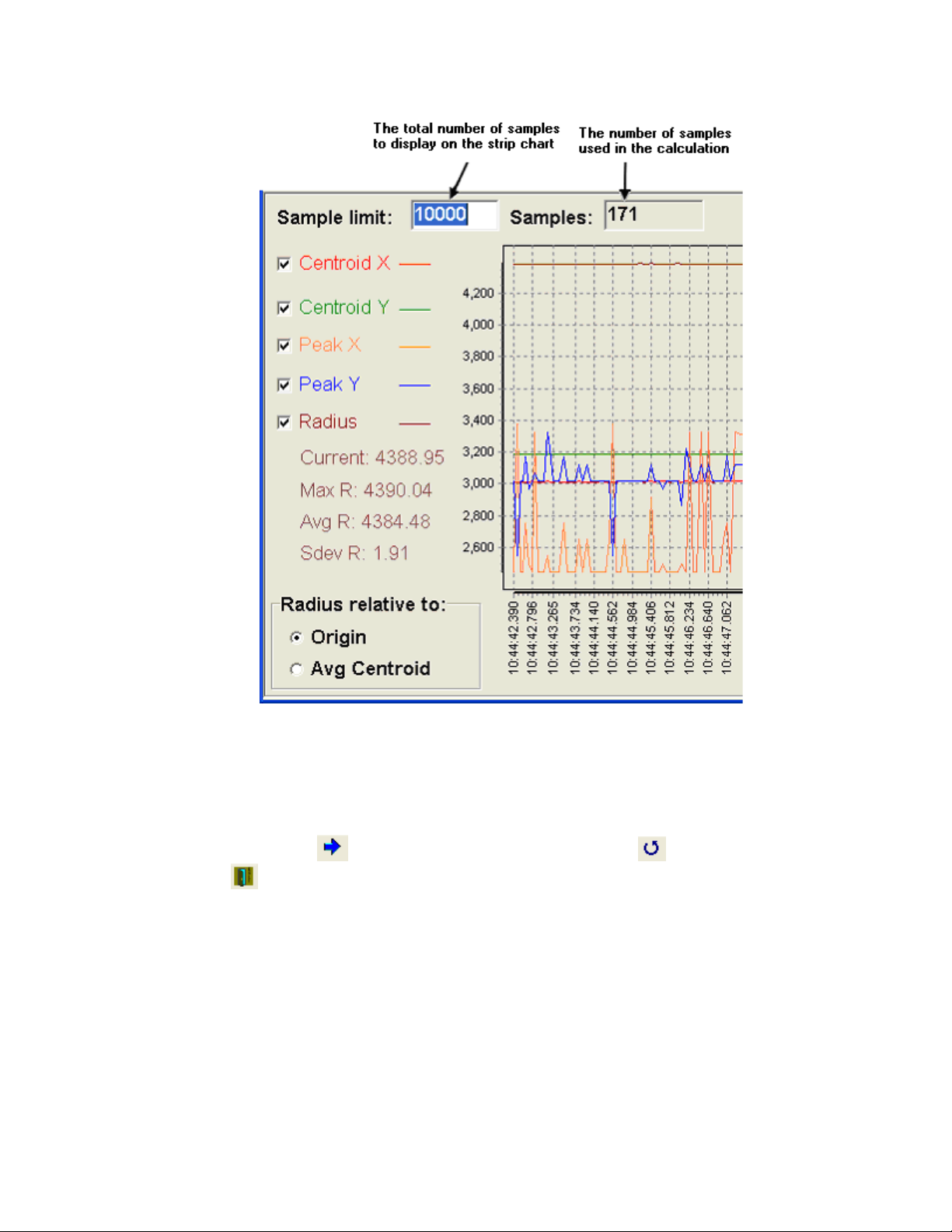
Figure 36
A sample of data is defined as; any results computed from a discrete beam image captured from
LBA-PC. The beam stability window will compute it’s results based on samples taken from the
time the Start arrow
is closed
and restarted.
is clicked, until the beam display is Reset , or until the application
3.2.9.2.1 Sample Limit
The strip chart display may become so compact that recent data points become visually indiscernible from the rest of the data in the strip chart. If the user desires to collect several samples, and still focus their attention on the most recent data, it may be necessary to limit the number of displayed samples. Sample limit edit box allows the user to specify how many of the most recent samples will be displayed in the strip chart.
Operator’s Manual LBA-PC
88
Page 89

Example: If the user has collected samples [1-1000] and the Sample limit it set to 100,
samples [900-1000] will be the only samples visible in the strip chart. Statistical results will
be computed using all the samples [1-1000].
3.2.9.2.2 Samples
The Samples indicator shows the total number of samples collected.
3.2.9.2.3 Check Boxes
The Check Boxes allow the user to specify what results items are to be graphed on the strip
chart. One or all of the following may be selected:
Centroid X
Centroid Y
Peak X
Peak Y
Radius
3.2.9.2.4 Radius Relative to:
The Radius Relative to control modifies the display of radius information. The radius is
referenced from an Origin set up in the LBA-PC or from the continuously calculated
Average Centroid position.
3.2.9.2.5 Strip Chart Zooming
All strip chart data is plotted on the same horizontal and vertical scale. This situation will
cause traces that vary greatly along the vertical axes to dominate the vertical scale. Traces
that have small vertical fluctuations will show up as flat lines. In order to see small details
the user must stop or pause the data collection and drag a zooming box around the region of
interest. To do this, start in the top left, drag a box spanning downward and to the right
until the region of interest is selected. More than one zoom operation may be performed to
achieve the desired detail.
Zooming out can only be done once. The plot will return to full zoomed-out mode. Zooming
out is accomplished by dragging a box from the bottom right back to the top left. The size of
the zoom-out box does not matter because all zoom out operations return the plot to the full
view.
Note: The direction of the zoom operation (in or out) is controlled by the direction the box is drawn, down and to
the right to zoom in and up and to the left to zoom out.
3.2.9.3 Peak/Centroid Scatter Plot and Histogram
There are two ways to use the Scatter Plots in the Beam Stability window. One is to test stability
from the standpoint of spatial dimension using units such as millimeters or microns. The other is
Operator’s Manual LBA-PC
Doc. No. 10654-001, Rev 4.10
89
Page 90

to use it as it relates to pixel units on the detector array. If you choose to do pointing stability
using spatial units such as mm or µm; the bins of the scatter/histogram plot and the horizontal
and vertical grid lines will not have any correlation to the individual pixels on the detector.
In other words, the bins in the histogram and the pixel grid of the detector will not have the
same crosshatch granularity. On the other hand, if you do it from the pixel-units standpoint, the
bins on the histogram will correlate with the size of the pixel grid on the detector. The
drawback however, is that you will be forced to multiply the results by the pixel scale of the
detector to get the data into real world units of distance.
The units on the horizontal and vertical axes of the scatter plots will change depending on how
you setup LBA-PC. They could be microns, millimeters, and fractions of pixels or any of the units
that are offered in LBA-PC. In short, the units on the X/Y-axes of the histogram/scatter plots are
the same as the units selected in LBA-PC for quantitative results. You can select these units by
going to LBA-PC’s main menu and selecting:
Options > Camera > Pixel Units
If, for example, you desired to see which pixels on the camera most often contained the peak of
your beam, setup your histogram bins to work in terms of individual camera pixels. To do this go
to the main menu on LBA-PC and select:
Options > Camera
From the camera dialog you would select the camera that matched your detector and then select
the Pixel Units to be PX (or pixel units). In the Pixel Scale spin control you would enter 1.0
to tell LBA-PC that your pixels are one pixel wide. Before closing the dialog you should make
sure that the Resolution drop down box is set to 1X. Resolutions other that 1X may be used
but this will be discussed later. In this example we will choose 1X because we do not want to
limit which pixels the peak might fall upon. Click OK to accept the changes to the camera dialog.
Now we will setup the origin in LBA-PC to match that of the histogram plot. On the main menu
select:
Options > Beam Display
Set the Origin Location to Window LL to coincide with the Beam Stability plot convention.
Setting the origin to values other that Window LL will work but the user should be aware that the
beam window and histogram might be horizontally or vertically inverted with respect to one
another.
Make sure that LBA-PC is collecting data and return to the Beam Stability window. Press the
reset button to restart the histogram.
Note: Whenever units are changed in LBA-PC, the scatter plot should be reset because previously plotted samples
will not be adjusted to reflect the new plot axis dimensions.
Operator’s Manual LBA-PC
90
Page 91

Figure 37
The Centroid and Peak Histogram windows now have horizontal and vertical plot scaling in units
of pixel, with histogram bins the size of a single pixel. Note also that we have the same plot
orientation as the LBA-PC beam window. In the Figure above we can see that most of the
centroids are falling 232
origin is set to Window LL). In order to get this into real world units we would simply multiply
the pixel units by the pixel scale of the camera. In the example above the pixel scale, read form
the camera dialog was 13 microns per pixel. Thus the centoid would become roughly:
pixels from the left and 247 pixels from the bottom (assuming that your
The ellipses in the histogram windows have X and Y diameters two standard deviations wide and
tall respectively.
Operator’s Manual LBA-PC
Doc. No. 10654-001, Rev 4.10
pixel
pixel
•
•
m
µ
pixel
m
µ
pixel
=
=
91
)(58.302413)(66.232 m
µ
From the left (X)
)(4.322113)(80.247 m
µ
From the bottom (Y)
Page 92

Figure 38
3.2.9.3.1 Zooming Histogram Plots
The zooming feature for histogram plots works basically the same as it does for the strip
chart window. (See Strip Chart Zooming)
3.2.9.3.2 Capture Resolution Settings.
When setting capture resolutions to settings other than Full and 1X, it is important to note
that the peak location scatter plot will not have peak locations on any pixel location in the
array. A 4X resolution for example, would have peaks occurring every forth pixel as a result
the Peak Scatter plot would look like something like the following figure:
Operator’s Manual LBA-PC
92
Page 93
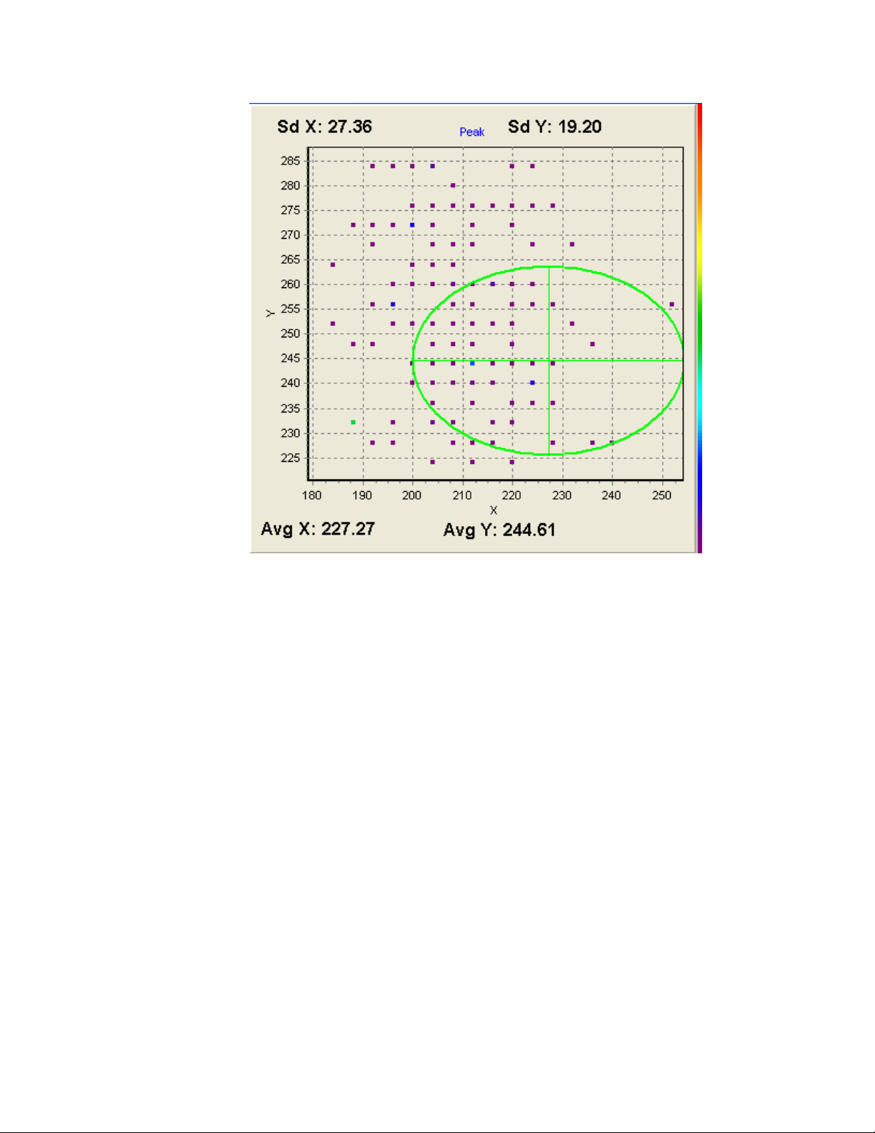
Figure 39
Note how peak locations seem to fall in a grid like pattern. This is to be expected when you are
capturing every 4
th
pixel.
3.2.9.3.3 Real World Units
Setting LBA-PC’s Quantitative results to real world units of length such as µm and mm may
be accomplished by going to the main menu and choosing:
Option > Camera
Make the appropriate real world unit selection in the Pixel Units drop down box. This
method of analyzing beam stability is in many ways similar to that discussed above however
when viewing the scatter plots the user must understand that the X/Y-axes will be in
whatever units are selected above. Also, the grid lines of the scatter plots will not have the
same granularity as the pixel grid on the detector. This method is best when scientific units
of length or beam centroid displacement are needed. When one understands the method
explained above this method should be intuitive. Remember to reset the scatter plot
whenever units are changed in LBA-PC.
Operator’s Manual LBA-PC
93
Doc. No. 10654-001, Rev 4.10
Page 94

3.2.9.3.4 Increment Bins and Reset
The centroid scatter-plot is also a histogram of the centroid location. The color bar between
the Peak and Centroid plots provides the user insight about centroid location/frequency.
Colors in the upper part of the bar indicate higher frequencies.
When running, the user will notice that blocks of data points have the same color. These
blocks of color represent the binning of the histogram. The program, based on the range of
data being presented, automatically defines the bin size.
If the user desires to decrease the size of the bins, simply click the Inc Bins button and the
bins will be divided in half both vertically and horizontally creating 4 bins out of each existing
bin. Bin size will be decreased when the program collects the next data point, and previously
plotted points will be re-plotted with respect to the new bin size. If the Pointing Stability
program is paused, the change will not take place until the program is started and the next
data point is collected.
3.2.10 Create Palette…
Clicking on this option will cause a separate color palette generation application to be launched. This
application will allow the user to design their own custom beam display color palette. Spiricon has
included a sample set of palettes that you can use or alter as you wish.
Using this tool, the user can easily create their own palettes, or modify the standard palettes provided
with Spiricon products.
The Spiricon Palette Generation program ( c:\Spiricon\LBAPC\PALETTEGEN2.EXE ) is shown below.
This program is very easy to use once a few concepts are understood. This program can be launched
independently via the Windows Start button, or from within the LBAPC application as follows: From
the Options menu select Create Palette…, the following window will appear:
Operator’s Manual LBA-PC
94
Page 95
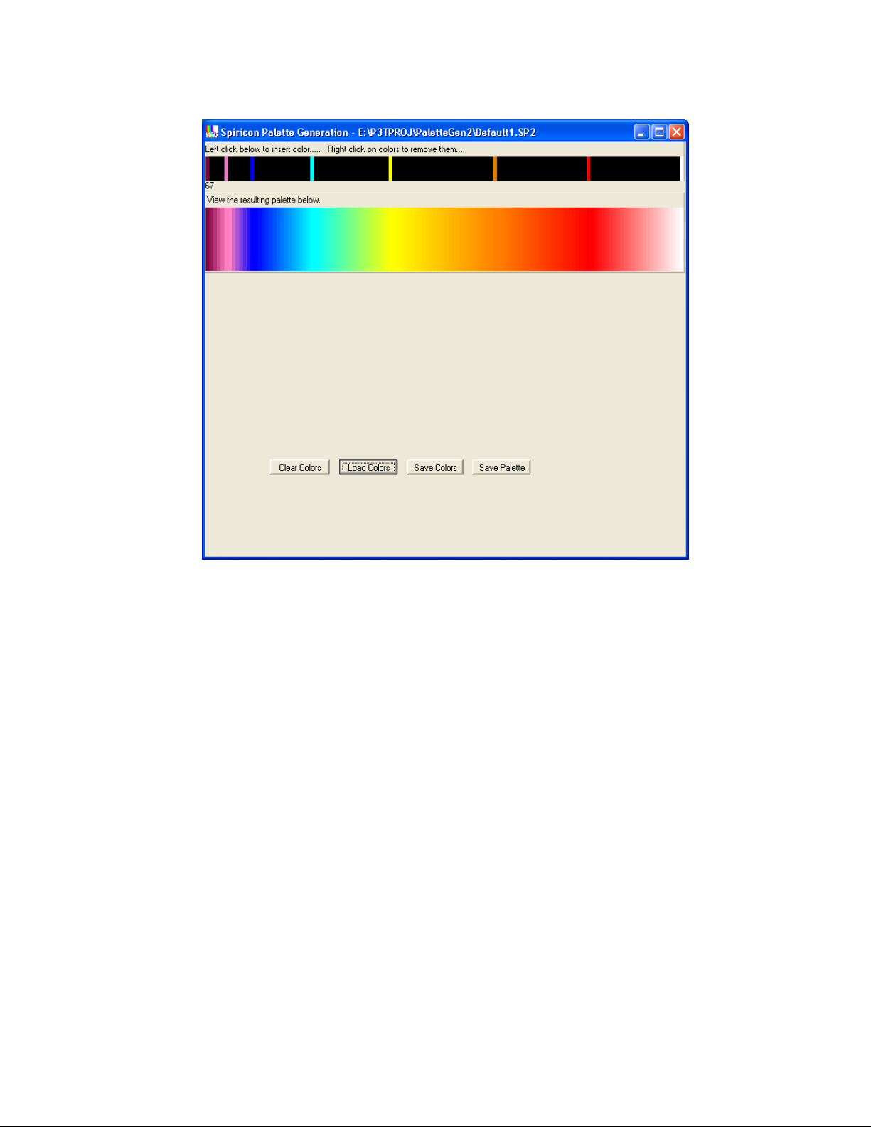
Figure 40
Upon opening, the above two horizontal color bars will be black. The designer can create a new
palette by placing seed colors into the upper bar and observing the resulting palette in the lower bar.
Colors on the left represent low intensities while colors on the right represent high intensities. The
upper bar contains entries for 128 individual colors, numbered from 0 on the left to 127 on the right.
You must define at least 2 colors to create a palette, or as many as 128 if you want to choose the
color of all possible displayed colors. LBA-PC uses a 128 color palette to describe all beam display
images, As you slide the mouse pointer along the upper bar a number (just below the upper bar) will
indicate which of the 128 color position is selected.
Left mouse clicking on a location in the upper bar will allow you to place a seed color at that physical
location. A Color selection dialog box will appear as shown below:
Operator’s Manual LBA-PC
95
Doc. No. 10654-001, Rev 4.10
Page 96
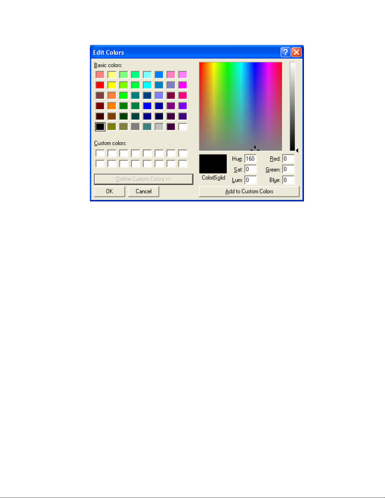
Figure 41
The user can either select one of the basic colors from the set on the left of the dialog, or create a
custom color using the controls on the right. Clicking OK will place the selected color into the upper
bar.
Continue to add seed colors until the displayed palette matches your desired effect.
To remove a seed color from the upper bar simply right-click on it.
3.2.10.1 Saving the Palette
Once you have the palette design looking the way you want it click the Save Palette button.
Enter the file name that you want the palette to be known by and save it into your
c:\Spiricon\LBAPC\Palette\ directory. The file extension .pal will automatically be applied.
3.2.10.2 Save Colors
The palette generation tools purpose is to create palettes of 128 entries, with minimal user input. Thus, the user may enter only 2 seed colors and the tool will interpolate the remaining colors. It is however difficult to move the other direction, that is to say, given a palette with 128 colors please reduce it to the original 2 seed colors. Therefore, a second file type was created to save the users seed colors for the purpose of editing later. This file type has a .sp2 extension. The Save Colors button is for the purpose of saving .sp2 file types or in other words, palettes that you can edit.
Operator’s Manual LBA-PC
96
Page 97

Note: Palettes saved as .pal file types cannot be loaded into the Palette Generation Tool (PaletteGen2.exe) for
editing!
3.2.10.3 Load Colors
The Load Colors button is used to load the seed colors from .sp2 files into the Palette Generation Tool for editing.
Note: Users should save a .sp2 file for each .pal file they desire to tweak at some later date.
3.2.10.4 Clearing Colors
Removes all seed colors and resets the palette display.
Operator’s Manual LBA-PC
Doc. No. 10654-001, Rev 4.10
97
Page 98

3.2.11 Password Lockout
You can enter a Password that will cause all of the LBA-PC setup functions to become inaccessible.
The password acts as a toggle. Type in the password once and all setup options will become
disabled. Type it in a second time and setup capability will be restored.
The password has been factory set. To find out your password call the Spiricon Service Department
at 435-753-3729 between the hours of 9:00 am and 5:00 pm MST. The password will only be given
out to an authorized individual. An authorized individual is one whose name appears on the original
Purchase Order, the person whose name appears on the completed warranty card, or to an individual
who knows the Purchase Order Number used to make the purchase. It can also be obtained by a
written request on your company letterhead, signed by an officer of the company.
3.3 Pass/Fail... Drop Down Menu Selections
3.3.1 Pass/Fail... enable and define its operation
All pass fail operations are enabled or disabled by checking the Master Enable box.
Figure 42
You can choose what Action(s) will be performed based upon if the results Fails or Passes the
designated tests.
Check the appropriate box to obtain these available actions:
• TTL Pulse: If you want the LBA to send a TTL pulse out the rear J5 connector, pin 1, each
time the Pass/Fail condition is met.
• Beep: If you want the LBA to cause your PC to Beep, each time the Pass/Fail condition is
met.
• Stop Running: If you want the LBA to halt and display the frame that caused the Pass/Fail
condition to be met.
Operator’s Manual LBA-PC
98
Page 99

3.3.1.1 PASS or FAIL results
The remaining Pass/Fail dialog boxes are used to set the Pass/Fail limits for the results items
that you want to test and screen for. When you check an item, you turn on the Pass/Fail
screening for that particular result. At the same time, you change how that result item will
appear in the results window. If a results item is being tested and it fails the test limits, the
displayed color will appear RED; if it passes the test limits, it will appear in GREEN.
3.3.1.2 Pass/Fail Units
The test units are always the same as what appears in the results window. If you redefine the
results window units, the set Pass/Fail values will not automatically rescale to the new settings.
In this case, you must manually change the Min. and Max. limits to meet the new unit
requirements.
3.3.1.3 Pass/Fail dialog boxes
The remaining Pass/Fail dialog boxes are very similar in how they allow you to select and set
limits for the result items that you want to test. In each instance you must:
1. Enable the results item by checking on its selection box.
2. Set the test limit values that are required.
In some instances you can select either or both Minimum and Maximum test limits.
Pass/Fail testing can only be performed on Current frame results. No Pass/Fail testing is allowed for Statistics
results.
Pass/Fail testing can only be performed on computational results that are enabled in the Computations dialog box.
Most of the Pass/Fail dialog box edit control items are obvious in their meaning, and how to set
them up. A few items are less obvious and are explained in the following sections.
3.3.2 Quantitative Pass/Fail
The following results may be set in the Pass/Fail Quantitative… dialog below the main menu
Pass/Fail item.
3.3.2.1 Min Fluence
The Min Fluence test is performed on the Min value in the Quantitative results display. This test is best applied in conjunction with a manually Drawn Aperture. It can be used to test for a Minimum fluence range of values over a specified region of your beam.
If your beam is a Top Hat, don’t use this test. Use the Top Hat Fluence setting in the Top Hat
Pass/Fail dialog box.
Operator’s Manual LBA-PC
Doc. No. 10654-001, Rev 4.10
99
Page 100

3.3.2.2 Centroid
The Centroid Pass/Fail item allows you to define a circle that must contain the centroid of the beam energy. To implement this test you must define the location of the center of a circle in terms of its X and Y coordinate in the beam display window, and the Radius of the circle that must contain it.
Both the X and Y Centroid location results will change color from GREEN to RED should the
centroid fall outside this circle.
3.3.3 Elliptical Pass/Fail
The following results may be set in the Pass/Fail Elliptical… dialog below the main menu
Pass/Fail item.
Figure 43
3.3.3.1 Orientation
The Orientation Pass/Fail item applies to the major axis inclination of an Elliptical beam. The units for these two edit controls are always in degrees. The Major axis can tilt through an angle in the range of +90 to -90 degrees. You can set the desired tilt Angle, and a +/- Range around this angle, that will meet your testing criteria. The Rotation result will change color from
GREEN to RED should the angle fall outside of these set limits.
3.3.4 Gauss Pass/Fail
See the Pass/Fail Gauss… dialog below the main menu Pass/Fail item for a list of these items.
3.3.5 Top Hat Pass/Fail
See the Pass/Fail Top Hat… dialog below the main menu Pass/Fail item for a list of these items.
Operator’s Manual LBA-PC
100
 Loading...