

Page 1

User Manual
Imaging Software
Life Science Microscopy
Imaging Software for
Life Science Microscopy
Page 2

Page 3

Imaging Software for
Life Science Microscopy
Software Manual for Imaging Stations
Version 1.1
Page 4

Page 5

Imaging Excellence
We at Olympus Soft Imaging Solutions GmbH have tried to make the information in this manual as
accurate and reliable as possible. Nevertheless, Olympus Soft Imaging Solutions GmbH disclaims
any warranty of any kind, whether expressed or implied, as to any matter whatsoever relating to
this manual, including without limitation the merchantability or fitness for any particular purpose.
Olympus Soft Imaging Solutions GmbH will from time to time revise the software described in this
manual and reserves the right to make such changes without obligation to notify the purchaser. In
no event shall Olympus Soft Imaging Solutions GmbH be liable for any indirect, special, incidental,
or consequential damages arising out of purchase or use of this manual or the information contained therein.
No part of this document may be reproduced or transmitted in any form or by any means, electronic or mechanical, for any purpose, without the prior permission of Olympus Soft Imaging Solutions GmbH.
© 2003 – 2010 by Olympus Soft Imaging Solutions GmbH. All rights reserved.
Page 6

OLYMPUS SOFT IMAGING SOLUTIONS GMBH
Rupert-Mayer-Strasse 44
D-81379 München
Tel: +49 89 - 89 55 805 660
Fax +49 89 - 89 55 805 6606
Email: info@olympus-sis.com
www.olympus-sis.com
Page 7

LICENSE AGREEMENT between END USER and OLYMPUS SOFT
IMAGING SOLUTIONS
PRODUCT.
IMPORTANT-READ CAREFULLY: Below you will find the contractual
agreements governing the use of the OSIS
SOFTWARE PRODUCT. These conditions apply to you, the user, and
to OLYMPUS SOFT IMAGING SOLUTIONS. With any of the following
actions you explicitly agree to be bound by the conditions of this
contract: purchasing the software, opening the package, breaking of
one of the seals or using the software.
In case you do not agree with any of the conditions of this contract,
please return all parts of the product including manuals and the
software protection key before using and without delay. Remove all
software installations of the product from any computer you might
have installed it on. Return all electronic media of the product or
completely destroy all electronic media of the product and send proof
that this has been accomplished. For a refund, please return everything to where you purchased the product.
§ 1. Scope
(1) This License agreement explicitly covers only the software diskettes or other media you received with the purchase and the software
stored on these media, the manuals, as far as they were developed
and produced by OLYMPUS SOFT IMAGING SOLUTIONS.
§ 2. User rights
(1) OLYMPUS SOFT IMAGING SOLUTIONS permits the User, for the
duration of this contract, to use the software on a single computer
and a single terminal on that computer. This license is explicitly nonexclusive, i.e., the User does not have an exclusive right to use the
software. As a licensed user you can copy the software from one
computer to another by using a computer network or other storage
devices, as long as it is assured, that the software can only be used
on a single computer or terminal at any time and that the conditions
set forth under § 4 are observed.
(2) The User has the right to produce a copy of the software only for
backup purposes.
§ 3. Additional user rights
Only if OLYMPUS SOFT IMAGING SOLUTIONS provides the User
with permission in written form the User can incorporate parts of the
software into other software developed by the User. A distribution of
the software can only be made in compiled form as part of the software developed by the User under strict observation of the conditions
set forth in the written permission to the User. The User must include
the OSIS
with the User's software. The User has to make sure, that OLYMPUS
SOFT IMAGING SOLUTIONS cannot be held liable for any damages
or injuries resulting from the use of the User's software, that include
parts of the OSIS
§ 4. Copyright
(1) OLYMPUS SOFT IMAGING SOLUTIONS or its subsidiaries remain
owners of the software and it's documentation. With the purchase,
the User obtains ownership of the diskettes or other physical storage
regarding the OSIS SOFTWARE
SOFTWARE PRODUCT copyright notification
SOFTWARE PRODUCT.
devices (excluding the software and other data contained thereon),
the manuals, and the software protection key.
(2) OLYMPUS SOFT IMAGING SOLUTIONS reserves the right to all
publications, duplication, editing, and marketing of the software and
the software documentation.
Without prior written permission the User may not:
– change, translate, de-compile or de-assemble the software,
– copy any of the written or printed documentation of the software,
– rent, lease, or license the software to a third party,
– use the software protection different than described in this contract.
(3) The license, property, and user rights to the OLYMPUS SOFT
IMAGING SOLUTIONS software, disks, and manuals may only be sold
or transferred to a third party on a permanent basis, if the third party
agrees to abide by the conditions in this contract.
(4) OLYMPUS SOFT IMAGING SOLUTIONS is the legal owner of all
copyrights and trademarks of the OSIS
PRODUCT and documentation. Copyrights and trademarks are
protected by national and international law. OLYMPUS SOFT
IMAGING SOLUTIONS reserves all rights, which are not explicitly
expressed in written form.
§ 5. Warranty
(1) OLYMPUS SOFT IMAGING SOLUTIONS guarantees for the period
of 12 months after the date of purchase, that the software works in all
major aspects according to the descriptions in the manuals.
OLYMPUS SOFT IMAGING SOLUTIONS, as the producer of the
software, provides this warranty. It does not replace or restrict other
warranties or liabilities provided to the User by local or other sales
people or organizations. OLYMPUS SOFT IMAGING SOLUTIONS
does not guarantee that the software is defect free; that the software
fulfills the specific requirements of the User, or that the OBS
SOFTWARE PRODUCT works with other software
provided by the User.
(2) OLYMPUS SOFT IMAGING SOLUTIONS further guarantees, that
the software storage devices (floppy disks, CD-ROMs, etc.) and the
manuals are free of material defects. Defective storage devices or
manuals will be replace free of charge, if they are returned to
OLYMPUS SOFT IMAGING SOLUTIONS within 90 days of purchase
and accompanied by a proof of purchase.
§ 6. Liability
(1) OLYMPUS SOFT IMAGING SOLUTIONS or their sales organizations cannot be held liable for damages or injuries resulting from the
use of the software or the lack of capabilities of the software, unless
the User can show gross negligence on the part of OLYMPUS SOFT
IMAGING SOLUTIONS. This applies, without exceptions, also to
losses of productivity or profit, interruptions in the flow of business or
manufacture, loss of information, and other financial losses. Without
exceptions the possible liability of OLYMPUS SOFT IMAGING
SOLUTIONS is limited to the amount that the User paid for the
product. These limitations on the liability do not influence claims for
reasons of product liability.
§ 7. Contract duration, legal consequences of violating the license
(1) The contract is deemed to be in force for an unspecified period.
The User rights are automatically terminated if one of the conditions
of the contracts has been violated.
SOFTWARE
Page 8

(2) In case of a contract violation the User has to return the original
storage devices and all copies thereof including all modified copies,
all printed and written documentation, and the software protection
key to OLYMPUS SOFT IMAGING SOLUTIONS, or the User has to
destroy these items.
(3) In addition OLYMPUS SOFT IMAGING SOLUTIONS reserves the
right to file a lawsuit to claim reparations for damages, noncompliance, or removal of the software in case of license violations.
The following laws and/or conditions are in effect: the conditions of
this contract, copyright laws, and the laws of the civil code.
Page 9

Software Manual Contents
3
7
9
0
0
9
0
9
0
6
7
9
0
Contents
Chapter 1
Imaging stations for life
science experiments
Chapter 2
A system chart and a list
of all components
1 Introduction ..................................................................................1
2
System Overview..........................................................................
2.1 System Chart....................................................................................4
2.2 Hardware..........................................................................................5
2.2.1 Motorized Microscope Modules....................................................... 5
2.3
Software ...........................................................................................6
Chapter 3
Getting you started – a
quick guide through the
main features of the
imaging stations and how
to use them
Chapter 4
Simple ways to take
images, how to control
the hardware modules
and which parameters to
set
3 Brief Introduction to the Software and First Steps...................
3.1 The User Interface .........................................................8
3.1.1 The Image Manager..........................................................................
3.1.2 The Viewport Manager ...................................................................1
3.1.3 The Viewport................................................................................... 1
3.2 Simple Image Acquisition ............................................................... 12
3.3 Saving Images – The Database ...................................................... 13
3.4 Loading Images .............................................................................. 14
3.5 Conducting Experiments with the Experiment Manager................ 14
3.6 Displaying Multi-Color Images .......................................................16
3.7 Displaying Sequences ....................................................................17
4 Image Acquisition and Hardware Control ..............................1
4.1 Simple Image Acquisition ............................................................... 20
4.1.1 Snapshot and Live View .................................................................2
4.1.2 AVI Recorder .................................................................................. 21
Camera Control ..............................................................................21
4.2
4.3 Illumination Control.........................................................................25
4.4 Microscope Control........................................................................26
4.5 Motorized Stage Control ................................................................29
4.5.1 Defining a Positions List .................................................................2
4.5.2 Correcting a Positions List .............................................................3
4.5.3 Calibrating the Motorized Stage..................................................... 32
4.6
Autofocus .......................................................................................34
4.6.1 Autofocus options…....................................................................... 35
Executing an Autofocus Scan ........................................................3
4.6.2
Chapter 5
Beyond snapshots:
setting up simple and
complex experiments in
an intuitive, graphical
way
5 Experiment Manager.................................................................. 3
5.1 A Graphical Tool ............................................................................. 38
5.2 Concept of Usage ..........................................................................39
5.2.1 Experiment Manager Components ................................................ 3
5.2.2 Arrangement and Customization.................................................... 4
5.3 Setting Up Experiment Plans .........................................................42
5.3.1 Types of Graphical Icons and the General Principles of Usage..... 42
5.3.2
The Command Symbols and Their Properties Pages ....................43
Page 10

Contents
0
7
0
0
4
4
6
6
9
6
6
8
8
9
9
0
3
4
4
6
8
9
9
0
0
5.3.3 Types of Experiments .....................................................................61
Conducting Experiments / Data Acquisition .................................. 70
5.4
5.4.1 Opening a Database .......................................................................7
5.4.2 Executing an Experiment ................................................................71
Data Storage and Preferences........................................................75
5.4.3
Chapter 6
Touching up the image
display by brightness,
contrast and color adjustment and navigation
through multidimensional image sets
6 Image Display and Navigation...................................................7
6.1 The Viewport .................................................................................. 78
6.2 Image Display................................................................................. 80
6.2.1 General............................................................................................8
6.2.2 Adjust Display…..............................................................................8
6.2.3 Auto Adjust......................................................................................8
6.2.4 White Balance .................................................................................8
6.2.5 Black Balance .................................................................................85
6.2.6
Gray Scale.......................................................................................85
Fluorescence Color.........................................................................8
6.2.7
6.2.8 Edit Fluorescence Color… ..............................................................8
6.2.9 False-Color… ..................................................................................87
Edit False-Color…...........................................................................8
6.2.10
6.3 Image Navigation ........................................................................... 95
6.3.1 General............................................................................................95
Multi-Color Images..........................................................................95
6.3.2
6.3.3
Displaying Different Color Bands in the Tile View Mode.................9
6.3.4 Time-Lapse Sequences ..................................................................9
6.3.5 Z-Stacks..........................................................................................9
6.3.6 Multi-dimensional Sequences.........................................................9
6.3.7 Parallel Navigation in Multiple Viewports........................................9
6.4 Projections and Extended Focal Imaging ...................................... 99
6.4.1 Projections Along the Z and Time Axes..........................................9
6.4.2 EFI – Extended Focal Imaging ......................................................10
6.5 Fluorescence and Transmission Image Overlay .......................... 101
6.6 Intensity Modulated Display......................................................... 102
Chapter 7
Basic processing routine
like size calibration,
overlay drawings, extraction and conversion of
image sets
7 Image Data Handling................................................................10
7.1 Calibrate Images .......................................................................... 104
7.1.1 Why Calibrate Images?.................................................................10
7.1.2 Calibrating the Camera Channel...................................................10
7.1.3 XY-Calibration...............................................................................10
7.1.4 Z-Calibration .................................................................................10
7.2 Scale Bar...................................................................................... 109
7.2.1 General..........................................................................................10
7.2.2 Setting the Scale Bar Properties...................................................10
7.2.3 Show in Viewport ..........................................................................11
7.2.4 Draw into Overlay..........................................................................11
7.3 Show Markers, Time and Z Information....................................... 111
7.4 Grid…........................................................................................... 111
7.5 Overlays ....................................................................................... 113
Page 11

Software Manual Contents
4
9
0
4
7
9
9
0
4
8
9
9
9
0
0
4
4
6
7.5.1 General ......................................................................................... 113
Activating the Overlay Toolbar .....................................................113
7.5.2
7.5.3
Creating and Editing Overlays...................................................... 11
7.6 Separate .......................................................................................118
7.7 Extract…....................................................................................... 118
7.8 Combine…....................................................................................119
7.8.1 General ......................................................................................... 11
7.8.2 Combining Data Sets ................................................................... 12
7.9 Convert Image ..............................................................................121
7.9.1 General ......................................................................................... 121
To 8-Bit......................................................................................... 121
7.9.2
7.9.3
To 16-Bit....................................................................................... 122
7.9.4
To RGB (3x8-Bit) .......................................................................... 122
Invert............................................................................................. 122
7.9.5
7.10
Image Information.........................................................................123
7.10.1 The General Tab ...........................................................................12
7.10.2 The Dimensions and Markers Tabs.............................................. 125
7.11
Image Statistics ............................................................................ 126
Chapter 8
Data changing tools to
improve the image quality, for example, by increasing the contrast or
reducing the noise
8 Image Processing ....................................................................12
8.1 Shading Correction.......................................................................129
8.1.1 General ......................................................................................... 12
8.1.2 Define Shading Correction ...........................................................12
8.1.3 Executing a Shading Correction................................................... 132
Bleaching Correction.................................................................... 133
8.2
8.3 Thresholds and Binarization ......................................................... 135
8.3.1 Set Thresholds.............................................................................. 135
Set Color Thresholds.................................................................... 14
8.3.2
8.3.3 Binarize......................................................................................... 14
8.4 Filters ............................................................................................ 145
8.4.1 General ......................................................................................... 145
8.4.2
Sharpen I ......................................................................................14
8.4.3 Sharpen II .....................................................................................14
8.4.4 Differentiate X ...............................................................................14
8.4.5 Differentiate Y............................................................................... 14
8.4.6 Laplace I .......................................................................................15
8.4.7 Laplace II ...................................................................................... 15
8.4.8 Mean............................................................................................. 151
8.4.9
Median.......................................................................................... 151
Pseudo Filter................................................................................. 152
8.4.10
8.4.11
Sobel ............................................................................................ 153
8.4.12
Roberts ......................................................................................... 153
Reimer ..........................................................................................15
8.4.13
8.4.14 User Filter .....................................................................................15
8.4.15 NxN............................................................................................... 15
8.4.16 Lowpass .......................................................................................157
8.4.17
Edge Enhance ..............................................................................157
Page 12

Contents
8
9
0
8
9
9
0
0
4
8
0
0
4
6
9
4
8.4.18 Rank ..............................................................................................15
8.4.19 Sigma ............................................................................................15
8.4.20 DCE – Differential Contrast Enhancement ....................................16
8.4.21 Separator ......................................................................................161
Morphological Filters.................................................................... 164
8.5
8.5.1 Define Morphological Filter... ........................................................165
8.5.2
Erosion ..........................................................................................167
Dilation ..........................................................................................16
8.5.3
8.5.4 Morph. Open.................................................................................16
8.5.5 Morph. Close.................................................................................16
8.5.6 Gradient ........................................................................................17
8.5.7 Top Hat Bright...............................................................................17
8.5.8 Top Hat Dark.................................................................................171
Distance Bright..............................................................................171
8.5.9
8.5.10
Distance Dark................................................................................172
8.5.11
Ultimate Erode Bright....................................................................172
Ultimate Erode Dark......................................................................173
8.5.12
8.5.13
Skeleton ........................................................................................173
8.5.14
Separate Particles.........................................................................17
8.6 Arithmetic Operations…............................................................... 175
8.7 Image Geometry .......................................................................... 177
8.7.1 Resize............................................................................................177
Rotate............................................................................................17
8.7.2
8.7.3 Mirror.............................................................................................18
8.7.4 Align ..............................................................................................18
8.7.5 Auto Align Z...................................................................................181
8.7.6
Shift Correction .............................................................................181
8.8
Deblurring and Deconvolution ..................................................... 182
8.8.1 General..........................................................................................182
8.8.2
Edit Image Parameters..................................................................182
8.8.3
No Neighbor..................................................................................18
8.8.4 Nearest Neighbors ........................................................................185
8.8.5
Wiener Filter ..................................................................................18
8.8.6 3-D AMLE Deconvolution: Advanced Maximum Likelihood .........187
Chapter 9
The software contains a
host of measuring tools
in a special measurement
environment
9 Measurements .......................................................................... 18
9.1 Measurements Toolbar ................................................................ 190
9.2 Drawing Tools for Length and Area Measurements .................... 191
9.2.1 Point..............................................................................................191
Touch Count .................................................................................191
9.2.2
9.2.3
Length ...........................................................................................192
9.2.4
Angle .............................................................................................19
9.2.5 Area...............................................................................................195
9.3
Magic Wand ................................................................................. 200
9.3.1 Magic Wand Options ....................................................................201
Results ......................................................................................... 202
9.4
9.4.1 Move Origin...................................................................................202
Page 13

Software Manual Contents
4
8
8
4
6
0
4
4
6
8
9
0
4
6
8
0
9.4.2 Create Measurement Sheet.......................................................... 203
Deleting Measurement Results..................................................... 20
9.4.3
9.4.4 Image Link ....................................................................................205
9.4.5
Show/Hide Statistic ...................................................................... 205
Select Measurements................................................................... 205
9.4.6
9.4.7
Define Statistics............................................................................ 207
9.4.8
The PreferencesMeasure Tab................................................... 20
9.4.9 Measurement Sheets: Statistics................................................... 20
Chapter 10
Sophisticated analyses of
fluorescence intensities,
mostly for time sequences and Z-stacks
10 Intensity Analyses ....................................................................211
10.1 Pixel Value ....................................................................................212
10.2 Histogram .....................................................................................213
10.3 Line Profiles: Intensity ..................................................................214
10.3.1 Horizontal Line Profile................................................................... 21
10.3.2 Vertical Line Profile....................................................................... 215
Arbitrary Line Profile .....................................................................215
10.3.3
10.3.4
Average Intensity of Neighboring Pixels....................................... 21
10.4 Regions of Interest – ROIs............................................................ 217
10.4.1 General ......................................................................................... 217
10.4.2
Drawing ROIs................................................................................ 217
10.4.3
ROI Measurements (2-D) .............................................................. 22
10.5 Background Subtraction... ...........................................................221
10.5.1 General ......................................................................................... 221
10.5.2
Subtracting the Image Background ............................................. 221
Intensity Kinetics in Time and Z ...................................................223
10.6
10.7 DeltaF / F (∆F/F) Analysis .............................................................224
10.7.1 General ......................................................................................... 22
10.7.2 Generating a (∆F/F) sequence ...................................................... 22
10.8 Ratio Analysis ...............................................................................226
10.8.1 General ......................................................................................... 22
10.8.2 Generating a Ratio Sequence ...................................................... 227
10.9
Spectral Unmixing ........................................................................228
10.9.1 Application.................................................................................... 22
10.9.2 The Problem ................................................................................. 22
10.9.3 The Solution.................................................................................. 23
10.9.4 How Does it Work?....................................................................... 231
Spectral Unmixing with .............................................. 232
10.9.5
10.9.6
Calibration ....................................................................................233
10.9.7
Unmixing....................................................................................... 23
10.9.8 Unmixing of Color Camera Images ..............................................23
10.10 Phase Color Coding and Analysis ................................................ 237
10.10.1 Phase Color Coding .....................................................................237
10.10.2
10.11 Colocalization ...............................................................................238
10.12 The FRET Software Module .........................................................240
10.12.1 Image Acquisition ......................................................................... 24
10.12.2 FRET Image Correction Factors................................................... 242
Phase Analysis ............................................................................. 23
Page 14

Contents
3
6
6
0
4
9
4
8
8
0
3
4
4
8
9
9
6
6
10.12.3 FRET Analysis ...............................................................................245
Kymogram.................................................................................... 251
10.13
Chapter 11
Analyses of intensity
kinetics of fluorescence
image time series
Chapter 12
Images generated during
an experiment are automatically stored in structured databases –
analytical data can be
added
Chapter 13
Setting personal preferences of the software
user interface
11 Graph Display and Graph Analysis .........................................25
11.1 Graph Documents........................................................................ 254
11.2 The Graph Window ...................................................................... 255
11.2.1 The Cursor: Changing the XY Scaling in the Diagram ..................255
11.2.2
The Cursor: Measuring Individual Graph Points ...........................25
11.2.3 The Graphs Button Bar .................................................................25
11.3 The Graph Menu .......................................................................... 260
11.3.1 Markers and Labels.......................................................................26
11.3.2 Protecting and Deleting a Graph ..................................................263
Graph Information... ......................................................................263
11.3.3
11.3.4
Sheet.............................................................................................26
12 Database ...................................................................................26
12.1 Directories for Data Storage ........................................................ 270
12.2 Open Database... ......................................................................... 271
12.3 New Database.............................................................................. 272
12.4 The Database Features................................................................ 273
12.4.1 General Remarks ..........................................................................273
12.4.2
The Database Window..................................................................27
12.4.3 Adjusting the Database Window...................................................275
Working with the Database.......................................................... 278
12.5
12.5.1 Loading Documents......................................................................27
12.5.2 Inserting Documents.....................................................................27
12.5.3 Query.............................................................................................28
12.5.4 Administration: Defining Organizational and Database Fields......281
13 The Special Menu and the Window Menu .............................28
13.1 Macros ......................................................................................... 284
13.1.1 General..........................................................................................28
13.1.2 Record Macro ...............................................................................28
13.1.3 Executing Macros .........................................................................285
Stop Macro Recorder ...................................................................287
13.1.4
13.1.5
Run Macro.....................................................................................287
13.1.6
Single Step....................................................................................287
Reset Interpreter ...........................................................................28
13.1.7
13.1.8 Set as Default-Macro ....................................................................28
13.1.9 Define Macros...............................................................................28
13.2 Add-In Manager... ........................................................................ 291
13.3 Define Menu Bar…....................................................................... 292
13.4 GUI Configuration ........................................................................ 295
13.4.1 Reset .............................................................................................29
13.4.2 Load... ...........................................................................................29
13.4.3 Save... ...........................................................................................297
Preferences... ............................................................................... 298
13.5
Page 15

Software Manual Contents
8
0
9
6
6
9
6
7
8
0
4
6
13.5.1 The PreferencesImage Tab....................................................... 29
13.5.2 The PreferencesView Tab .........................................................30
13.5.3 The PreferencesFile Tab ........................................................... 302
13.5.4
The PreferencesMeasure Tab................................................... 307
The PreferencesModule Tab..................................................... 30
13.5.5
13.5.6 The PreferencesGraph Tab....................................................... 311
13.5.7
The PreferencesDatabase Tab ................................................. 312
Window......................................................................................... 313
13.6
13.6.1 Minimize All................................................................................... 313
13.6.2
Close All........................................................................................ 313
Document Manager… ..................................................................313
13.6.3
13.6.4
Viewport Manager ........................................................................315
13.6.5
Image Manager............................................................................. 315
Status Bar..................................................................................... 31
13.6.6
13.6.7 Command Window....................................................................... 31
Chapter 14
A complete, integrated
development environment for macros based
on the programming
language Imaging C
Chapter 15
Telling the software
which hardware modules
are available and what
the current installation is,
for example, what filters
are loaded
14 Imaging C ..................................................................................31
14.1 General .........................................................................................320
14.2 New Module... ..............................................................................321
14.3 Open Module................................................................................327
14.4 Add to Module..............................................................................328
14.5 Save Module Configuration .......................................................... 329
14.6 Edit Module... ...............................................................................330
14.7 Build Module ................................................................................331
14.8 Close Module ...............................................................................332
14.9 About Module ............................................................................... 332
14.10 Module Manager... .......................................................................333
14.10.1 The Define Search Path for Modules Dialog Box ......................... 33
14.11 Browser... .....................................................................................337
14.12 Find Symbol..................................................................................338
14.13 Goto Definition.............................................................................. 339
14.14 Quick Watch... ..............................................................................340
14.15 Watch Variables............................................................................ 341
14.16 Toggle Breakpoint ........................................................................342
14.17 Edit Breakpoints ...........................................................................344
15 Configuration........................................................... 34
15.1 The Illumination System MT20 / MT10.........................................348
15.1.1 Configuring the Excitation Filters .................................................34
15.1.2 Burner Configuration .................................................................... 35
15.1.3 Using MT20 / MT10 without the Imaging Software...................... 351
Configuring the Microscope ......................................................... 351
15.2
15.2.1 General Configuration .................................................................. 351
15.2.2
Z-Drive Configuration ................................................................... 353
Configuration of the Objectives.................................................... 35
15.2.3
15.2.4 Configuration of the Fluorescence Filter Turret............................ 355
15.2.5
Configuration of the Transmission Contrast Inserts..................... 35
Page 16

Contents
6
9
Configuration of the Filters of a Filter Wheel.................................357
15.2.6
Definition of Image Types ............................................................ 358
15.3
15.4 Configuration of Additional Shutters............................................ 360
15.5 Configuration of the PIFOC.......................................................... 361
15.6 Configuration of the Motorized Stage.......................................... 362
15.7 The UCB Control Box Light Panel ............................................... 363
15.8 Parfocality Correction of Objectives ............................................ 364
15.9 Configuration of the DV2/Dual-View™ Micro-Imager.................. 365
15.9.1 Configuring the Emission Filters ...................................................36
15.9.2 Configuring the Image Types........................................................367
Chapter 16
The details to take care
of when installing a new
software version
16 Installing the Software ...........................................36
16.1 Updating the Software............................................... 370
16.2 Updating the Hardware Control ................................ 372
16.3 Selecting the Camera................................................................... 373
16.4 Single-User Systems (Administrator Users)................................. 374
16.5 Multi-User Systems...................................................................... 375
16.6 PC-to-Controller Network Connection ........................................ 377
Page 17

Software Manual Chapter 1 – Introduction 1
1 Introduction
Thank you very much for purchasing Olympus' state of art
confidence in our products and service. It is Olympus' main objective to provide you with solutions
able to meet your experimental demands and thus pave the way to your scientific success.
Imaging Station and for your
Page 18
2 Chapter 1 – Introduction
Introduction
The concept and technology of introduces the next generation of imaging workstations.
is designed as a modular imaging system for a broad range of life science experiments
that supports the Olympus microscopes of the IX and BX series.
successor of the cell^M /cell^R Imaging Software 3.3.
Hallmarks of the systems are:
• The unique all-in-one Illumination System MT10 or MT20 for fast wavelength switch and at-
tenuation to meet the experimental requirements for fast real-time acquisition by highly sensitive
digital cameras.
• The Real-Time Controller of
synchronize the all the hardware devices and modules. This additional independent plug-in CPU
board assures highest accuracy in experiment timing (temporal resolution: 1 ms; precision <
0.01 ms). In practice this ensures that illumination of the specimen can be strongly limited to the
acquisition of the image. As a consequence bleaching and photo damage of the specimen can
be minimized.
• The System Coordinator of
all the hardware devices and modules (temporal resolution: 1 ms). It carries out all the tasks that
the Real-Time Controller does, but lacks its timing precision and ability to run all tasks in parallel.
• The sophisticated
tures an intuitive and user-friendly graphical drag-and-drop interface, the Experiment Manager,
for setting up and executing even the most complex experiments in a convenient and concise
way. A structured database for multi-dimensional data handling (xyz, time, color) is also included, as well as tools for image processing, image analyses, and more complex analysis, like
rationing, ∆F/F, FRET, and spectral unmixing. The integrated Imaging C Module and Macro Recorder give the opportunity for advanced users to customize applications and automate functions.
This manual is the complete documentation necessary for using the Olympus imaging station
correctly and efficiently.
imaging software is a powerful all-embracing platform that fea-
real-time systems, a hyper-precision control board to
professional systems, a control board to synchronize the
1.1 is the immediate
Special care has been undertaken for this manual to guarantee correct and accurate information,
although this is subject to changes due to further development of the
Thus, the manufacturer cannot assume liability for any possible errors. We would appreciate reports of any mistakes as well as suggestions or criticism.
If you find any information missing in this manual or you need additional support, please contact
your local Olympus dealer.
imaging station.
Page 19

Software Manual Chapter 2 – System Overview 3
2 System Overview
The following chapter gives you a short overview of the basic
out additional peripherals). The system consists of different hardware and software devices, which
are full, integrated.
system components (with-
Page 20
4 Chapter 2 – System Overview
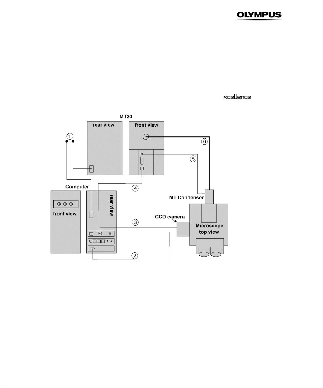
2.1 System Chart
The system chart shown exemplifies the different components of a standard system and
how they are interconnected.
Page 21

Software Manual Chapter 2 – System Overview 5
2.2 Hardware
The hardware devices of the imaging station are listed below:
• Olympus microscope of the IX or BX series, according to your specification.
• CCD camera (Olympus XM10T, Hamamatsu ORCA-R2 or other) or EMCCD camera (Hamamatsu
C9100-13, Andor iXon or other)
• Illumination System, typically MT10 / MT20 bearing the arc burner (150W Xe or 150W Xe/Hg),
the motorized filter wheel (8 positions), attenuator and shutter.
• System Coordinator / Real-Time Controller for multi-task acquisition: bears an I/O panel with
seven BNC plugs to trigger peripherals, RS-232 socket to integrate external devices such as
motorized stages, analog OUT for piezo objective or nosepiece movers (PIFOC) and an Olympus
Device Bus (ODB) interface for fast filter wheels, mirror unit turret and transmission shutter.
• Computer: latest generation PC with all standard features, modified for hardware control and
peripherals integration, monitor.
• System-specific accessories (filter sets etc.).
2.2.1 Motorized Microscope Modules
supports the following motorized IX2 and BX2 microscope components:
• z-drive
• fluorescence filter turret
• transmission condenser
• nosepiece
• ocular-to-camera switch
• bottom-to-side port switch
• observation filter wheel
• transmission shutter
Page 22

6 Chapter 2 – System Overview
2.3 Software
• ObsConfig Configuration Software to configure the Illumination System MT10 / MT20.
•
experiments, Viewport, Viewport Manager, and Image Manager for managing and displaying the
images on the desktop, Image and Graph Analysis tools to analyze the acquired data, and a database for storing and archiving the images.
•
Controller and the MT10 / MT20 electronics
Imaging Software integrating the Experiment Manager for planning and executing
software updates only: Update Software for the System Coordinator / Real-time
Page 23

Software Manual Chapter 3 – Brief Introduction and First Steps 7
3 Brief Introduction to the
Software and First Steps
The following sections explain the basic features and functions. They also introduce the
most important terms used in the software and in this manual and thus should help you to get
started.
For you to follow the contents of this chapter it is necessary that the system (hardware and software) has been installed and properly configured. For a detailed description of the system installation and configuration read Chapter 15,
the Hardware Manual, especially Chapter 7, System Assembly and Adjustment.
3.1
The User Interface ..........................................................8
3.1.1 The Image Manager.......................................................................... 9
3.1.2 The Viewport Manager ...................................................................10
3.1.3 The Viewport...................................................................................10
3.2 Simple Image Acquisition ............................................................... 12
3.3 Saving Images – The Database ...................................................... 13
3.4 Loading Images .............................................................................. 14
3.5 Conducting Experiments with the Experiment Manager................ 14
3.6 Displaying Multi-Color Images .......................................................16
3.7 Displaying Sequences ....................................................................17
Configuration, of this manual carefully as well as
Page 24
8 Chapter 3 – Brief Introduction and First Steps
fff
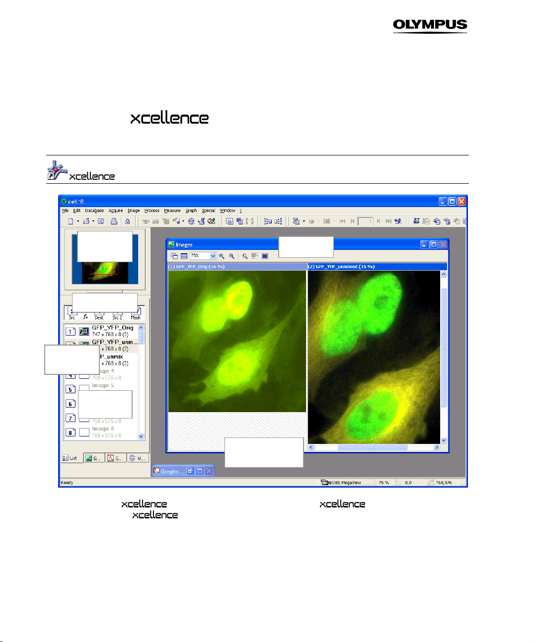
3.1 The User Interface
feerr BBooxx
DDooccuummeenntt
AArreeaa
VViieewwppoorrtt
icon on your desktop to start the software or open it via
. The screenshot below shows the program's graphical user inter-
VViieewwppoorrtt
MMaannaaggeerr
OOppeerraannddss BBooxx
IImmaaggee
MMaannaaggeerr
IImmaaggee
u
BBu
Double-click the
StartPrograms
face (GUI). It is composed of:
a Menu bar: access to pull-down menus with assorted commands.
b Tool bar: direct access to the most important commands for image acquisition, processing and
analysis.
Page 25
Software Manual Chapter 3 – Brief Introduction and First Steps 9
c Status bar: shows the connected CCD camera and displays information depending on the ac-
tive functions.
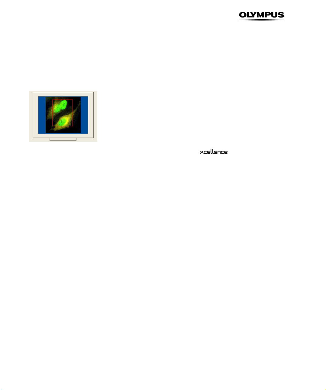
d Viewport Manager (top left below button bars): shows a thumbnail of the active image; a red
rectangle indicates the current zoomed-in sector of the image in the Viewport. The rectangle
can be mouse-dragged across the thumbnail to bring a different area into display.
e Image Manager (underneath the Viewport Manager): consists of two parts:
— the Operand Box, an operational area to determine source and destination buffers for
image processing
— the Image Buffer Box listing the currently loaded images or graphs. Four tabs are
available:
1 The List View that lists the names, the XY size and the bit depth of the images.
2 The Gallery View that shows thumbnails of the images.
3 The Graph View that shows thumbnails of loaded graphs.
4 The Measurement View that lists the results of area and length measurements in
images.
f Documents Area which always contains:
g Viewport: displays the active image or a selection of currently loaded images.
h Graph document: the currently active graph (if a corresponding analysis has been carried out).
It is minimized when
is started.
i Additionally the Documents Area may contain:
j Database Documents
k Data Sheets
l Text Documents and Macros
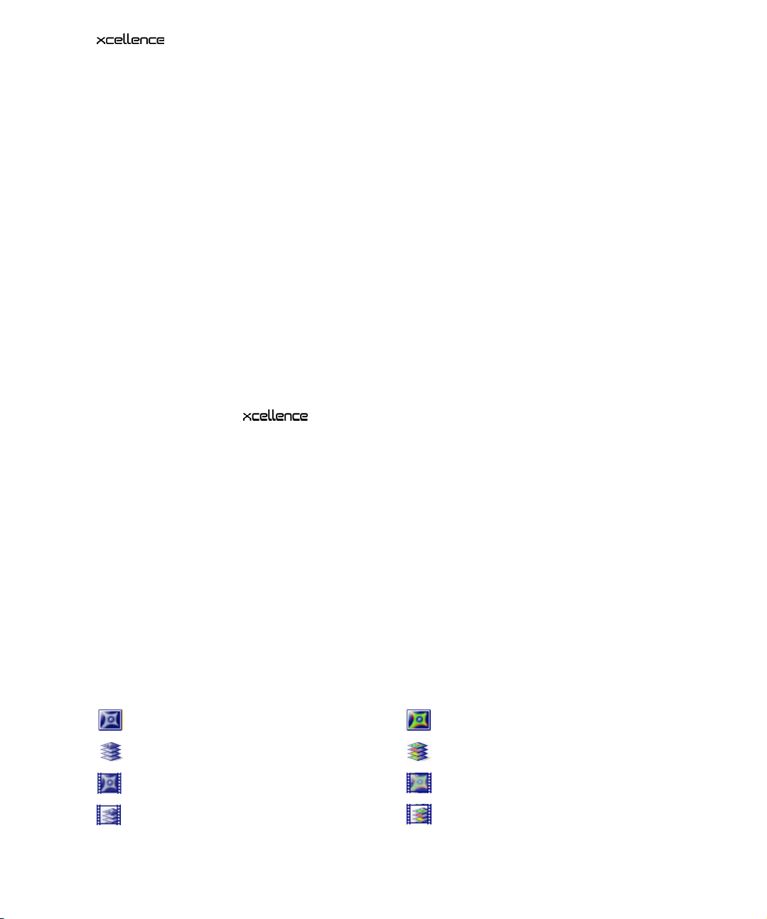
3.1.1 The Image Manager
In the Image Manager different image types, like single color images, multi-color images, or the
various image sequences (z-stack; time-lapse, etc.), are represented by different symbols.
The highlighted image frame in the Image Manager field is active and displayed in the Viewport
Manager and the Viewport.
single-color image
Z-stack
single-color time-lapse
single-color Z-stacks in time-lapse
multi-color image
multi-color Z-stack
multi-color time-lapse
multi-color Z-stacks in time-lapse
Page 26
10 Chapter 3 – Brief Introduction and First Steps
3.1.2 The Viewport Manager
The image in the Viewport Manager in the top left corner of the
rectangle. It represents the region of the image currently displayed in the Viewport – if the image is
zoomed to an extent that is larger than the Viewport. The rectangle is interactive: It can be freely
moved within the Viewport Manager to display different areas in the Viewport. It can also be resized
by mouse drag to change the zoom factor in the Viewport display.
window shows a red
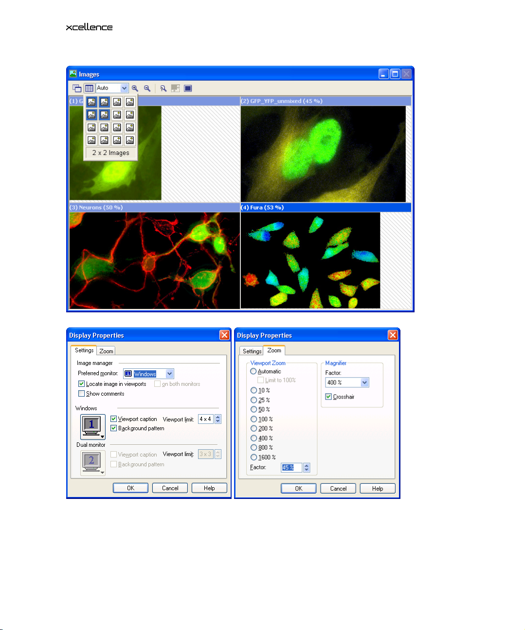
3.1.3 The Viewport
The Viewport window allows displaying one image or a number of images at the same time. The
number of Viewports to be displayed and their arrangement can be set using the Arrange View-
ports button in the toolbar of the Image window. Just mark the columns and rows by moving the
mouse cursor over the schematic Viewport, which opens with 4x4 image icons symbolizing independent image areas. The maximum number of images that can be shown at one time is 16 (4x4)
by default.
This setting can be increased to 5x5 as maximum via the Display Properties. Right-click on the
Viewport Manager to open the Display Properties window and change the Viewport limit entry
accordingly.
Page 27
Software Manual Chapter 3 – Brief Introduction and First Steps 11
Page 28

12 Chapter 3 – Brief Introduction and First Steps
3.2 Simple Image Acquisition
Live View, Snapshot, Camera Control, Illumination Settings
The most important tools for simple image acquisition are the Live View and Snapshot buttons
and the control boxes that are opened by the Camera Control and Illumination Settings buttons;
all can be found in the Acquisition toolbar.
In the following a typical procedure for the acquisition of a fluorescence image will briefly be described. For detailed explanations, see Chapter 4, Image Acquisition and Illumination Control.
Make sure to select the correct objective and fluorescence filter and place your sample on the
stage. The usage of the microscope will not be explained here.
1. Click Illumination Settings to open the Illumination system MT20 / MT10 control box.
2. Click Main switch / Burner ON to ignite the burner. (For a stable light output, wait about
10 min.)
3. Click on one of the Excitation filter buttons to select an illumination color.
4. Click Camera Control to open the corresponding window. Reasonable starting settings
are:
– Binning 2x2
– Exposure time 50 ms
– Brightness adjustment automatic
These settings have to be adjusted in the course of the working session.
5. Direct the light path of the microscope to the camera. (Of course, focusing can be done
via the ocular, but this will not be explained here.)
6. Click Shutter in the Illumination System MT20 / MT10 control box to illuminate the
specimen.
7. Click Acquire in the Acquisition toolbar or the Camera Control window. The following
happens:
Page 29

Software Manual Chapter 3 – Brief Introduction and First Steps 13
– The camera starts acquiring images at maximal speed. None is stored; instead, the
newest image overwrites the previous one in the temporary buffer.
– The current image is displayed in the active Viewport.
– A single image icon appears in the Image Buffer Box.
8. Focus your sample with the microscope Z-drive. (Even if the optional PIFOC is available
for focus change, its total range may be too narrow to find the focus at the beginning.
For this reason it is usually better to start with the Z-drive.)
9. If necessary, change the Binning factor in the Camera Control window: 1x1 in order to
get highest spatial resolution, larger factors increase the signal intensity at the cost of
resolution.
10. Adjust the Exposure time for a good signal-to-noise ratio.
11. Click Snapshot in the Acquisition toolbar or the Camera Control window to stop the
Live View. The very last image is being stored as a Snapshot in the Image Buffer Box
and displayed in the Viewport.
12. Click Shutter in the MT20 / MT10 control box to stop the illumination.
13. Save your image as described in the next chapter.
Select an empty buffer in the Image Manager if you want to acquire a new image, otherwise the current image will be overwritten and lost: snapshots are only stored temporarily and need to be saved.
3.3 Saving Images – The Database
To save a snapshot in the most basic way select FileSave from the menu bar or use the short cut
<Ctrl + s>. The snapshot will be stored in a 16-bit tiff format by default. Other data types can be
chosen as usual in the Save Image As window. As with other files, you have to give a name and
select the destination (path) of the storage.
features a database module for the storage of images and entire experiments including
Experiment Plans, data sets, analyses and so on. The module is explained in detail in Chapter 12,
Database.
Page 30
14 Chapter 3 – Brief Introduction and First Steps
The command Open Database… to load an existing one can be found redundantly in the menus
File, Acquisition and Database. Database files carry the extension *.apl. New databases can be
created with the command New Database…, to be found in the same menus.
In order to be able to store your images in the database, first you have to create an experiment
folder via DatabaseInsertExperiment… (or use an existing one). To store an image in the
database just drag it from the Image Buffer Box into the experiment folder. You will be asked in a
dialog box to give it a name.
Images acquired via the Experiment Manager will be stored automatically in a database.
3.4 Loading Images
To load images that are not stored in a database and to display them in the Viewport use the command FileOpen (short-cut <Ctrl + o>) or click on the Open button in the toolbar. As usually you
have to navigate to the storage folder of the file and select it.
Open the experiment folder in the database to load an image or an image sequence from it (see
previous chapter 3.3). In the Structure Strip on the left hand side of the database window you will
find the Image Icon and in the Gallery Field – the Image Thumbnail. Drag either the icon or the
thumbnail into the Viewport or the Image Manager to load the image set.
3.5 Conducting Experiments with the Experiment
Manager
Experiment Manager
In general, most imaging applications in life science are rather complex and go beyond taking simple snapshots, for example, multi-color imaging, time-lapse imaging, ion imaging with ratiometric
fluorescence dyes, multi-dimensional imaging, etc. The
Experiment Manager, an easy-to-use and intuitive tool to plan, configure and execute even the
Imaging Software includes the
Page 31

Software Manual Chapter 3 – Brief Introduction and First Steps 15
most complex experiments without any programming knowledge. The Experiment Manager is explained in every detail in chapter 5. In the following only a brief introduction will be given.
To open the Experiment Manager click the Experiment Manager button in the acquisition toolbar.
Experiment Plans are set-up by assembling and connecting diverse command icons and frames.
The most frequent ones can be selected via buttons in the Standard Command toolbar and
placed into the editing area by drag&drop.
Image Acquisition, Multi-Color, Z-Stack and Time Loop
A Properties page to specify certain settings accompanies each command icon that is placed into
the editing area. In case of Image Acquisition, for example, parameters such as exposure time
and excitation filter have to be set.
The scheme below is just one example of an experiment plan. It shows the command icons that
define a multi-color time-lapse experiment. There are three Image Acquisition icons, each with a
different excitation filter, surrounded by a multi-color frame for combination of the three Image
Types (monochrome images) to one multi-color image. The outer frame represents a Time Loop to
repeat all commands contained a certain number of times.
The Experiment Manager is not only a tool to design the experiments, but also the command center
to acquire the images according to the Experiment Plan. The necessary icons are grouped in the
Control Center toolbar.
Check!, System Ready!, Start!, Pause and Stop
The execution of an Experiment Plan involves three steps:
1. Check!: The system verifies if the execution of the Experiment Plan is feasible or if there
are invalid parameters or logical faults.
2. System Ready!: The Experiment Plan is downloaded to the Real-Time Controller and
data storage space is allocated on the hard disk.
Page 32

16 Chapter 3 – Brief Introduction and First Steps
3. The experiment itself is started, paused and stopped with Start!, Pause, and Stop.
Any image or image sequence acquired with the Experiment Manager is automatically
stored on the hard disk in a database.
3.6 Displaying Multi-Color Images
Select Color Channel
Multi-color images consist of several color channels – in principle the number is unlimited. Each channel contains a monochrome image of predefined color resulting from one Image
Acquisition command in the Experiment Plan. When loaded from an archive all color channels are
displayed together in an overlay resulting in a color image. The Select Color Channel button in the
Navigation toolbar provides a tool to navigate easily through all color channels and to display selected ones.
Display Intensity
Adjusting the single color intensities with the dialog box of the Display Intensity command can
optimize the look of the multi-color image. For details, see Chapter 6.2.2, Adjust Display.
Page 33

Software Manual Chapter 3 – Brief Introduction and First Steps 17
3.7 Displaying Sequences
Navigation
Time-Lapse experiments and Z-stack acquisitions generate series of images that are all stored
together within one file. The individual images can be accessed with the navigation buttons (First,
Previous, Next, Last) in the Navigation toolbar. The number in the Go To field represents the
actual frame displayed in the Viewport.
An additional feature enables the user to animate image sequences and play it as a movie. Pressing
the Animate button opens the Animate Image Stack window.
, Animate
Here you find the buttons to start (Play) the animation, to Stop it and to play it in the Reverse
mode.
Reverse, Stop and Play
For a detailed description of the navigation tools see Chapter 6.3, Image Navigation.
Page 34

18 Chapter 3 – Brief Introduction and First Steps
Page 35

Software Manual Chapter 4 – Image Acquisition and Hardware Control 19
4 Image Acquisition and
Hardware Control
The following chapters explain how to take snapshots or live images, what camera parameters
have to be adjusted for good quality and how to use the illumination system with the excitation
filters and the motorized parts of the microscope.
4.1
4.1.1 Snapshot and Live View .................................................................20
4.1.2 AVI Recorder .................................................................................. 21
4.2 Camera Control ..............................................................................21
4.3 Illumination Control.........................................................................25
4.4 Microscope Control........................................................................26
4.5 Motorized Stage Control ................................................................29
4.5.1 Defining a Positions List .................................................................29
4.5.2 Correcting a Positions List .............................................................30
4.5.3 Calibrating the Motorized Stage..................................................... 32
4.6 Autofocus .......................................................................................34
4.6.1 Autofocus options…....................................................................... 35
4.6.2 Executing an Autofocus Scan ........................................................36
Simple Image Acquisition ............................................................... 20
Page 36

20 Chapter 4 – Image Acquisition and Hardware Control
4.1 Simple Image Acquisition
4.1.1 Snapshot and Live View
Snapshot, Live View
There are two ways to achieve simple image acquisition. The first one is the acquisition of a single
image with the Snapshot button in the Acquisition toolbar or the Camera Control (or Acquisi-
tionSnapshot). The second one is the live view started with the neighboring Live View button (or
AcquisitionLive). Here the displayed image is updated continuously (and the previous image
discarded). Pressing the Snapshot button stops the Live View image display; thus a final snapshot
is taken, which remains in the image memory.
Snapshots are displayed with the false color defined for the currently active Image Type; see
Chapter 4.4, Microscope Control.
The Live View image is displayed in gray scale unless the option ImageImage Dis-
playFluorescence Color is activated. In that case the false color defined for the currently active
Image Type is used.
uses the current camera control and display settings for image acquisition. It remembers the settings from your last session after program shutdown and restart. Please be aware that
in case the properties of your object (dye, intensity, background etc.) have changed significantly, it
might be necessary to adjust the camera control and display settings accordingly before you can
see a reasonable image. This is explained in the following chapters.
The following settings should be checked or corrected before the image acquisition is started:
• Exposure time (Camera Control)
• Binning factor (Camera Control)
• Brightness adjustment (Camera Control)
• Image size, i.e., full frame or area of interest/partial frame (Camera Control)
• Excitation filter (Illumination Control)
• Light intensity (Illumination Control)
By default, snapshots are not being stored and also a new snapshot overwrites the
older one. These settings can be changed, however, see Chapter 13.5.1 The Prefer-
encesImage Tab.
Page 37

Software Manual Chapter 4 – Image Acquisition and Hardware Control 21
4.1.2 AVI Recorder
This function is not active after a standard installation of the software. Execute SpecialAdd-In Manger. Click Add in the corresponding window and navigate to the
gram folder. Open AviRec.dlx. Close the Add-In Manger window and restart the program. The
Acquisition toolbar now contains the Start/Stop Avi recording button.
Start/Stop Avi recording
Click the Start/Stop AVI recording button to have the current live image be acquired as a video.
During the acquisition, the settings in the AcquireAVI Recording Options dialog will be used.
Click on the Start/Stop AVI recording button once more or the Snapshot button to end the acquisition process.
The results of the acquisition will be saved on your hard disk in the form of a video file (AVI file).
You can edit the name and storage location in the AVI Recorder Options dialog box. In the image
document you will still see the live image.
The video file that you create can become very large. Make sure that there is sufficient
free space on your hard disk before you begin the acquisition and use a suitable compressor.
pro-
4.2 Camera Control
Camera Control
The Camera Control button (or AcquisitionCamera settings...) opens the window to set the
acquisition parameters Exposure time, Binning factor and Subframe as well as the principal image display parameters. The Camera Control window can be moved freely across the screen.
The
parameters during Live View, which makes it very convenient to adjust the acquisition for each
experiment.
The Camera Control window contains the same Snapshot and Live View buttons as the Acquisi-
tion toolbar described in Chapter 4.1, Simple image Acquisition.
Imaging Software provides the unique possibility to change all the above mentioned
Page 38

22 Chapter 4 – Image Acquisition and Hardware Control
Snapshot, Live View
Binning. The CCD chip is composed of many light-sensitive units (pixels). These pixels can be read
out individually (binning = 1x1) or the signal of neighboring pixels can be combined electronically
on the CCD chip (binning > 1x1). Binning reduces the spatial resolution but increases the sensitivity
and thus reduces the exposure time required for a good signal-to-noise ratio. It further reduces the
amount of data and consequently increases the readout speed. Therefore binning is recommended
if weak signals have to be detected at high acquisition rates or if spatial resolution is of minor importance. .
Exposure Time. The exposure time determines the period of time during which the CCD-chip is
sensitive to incoming light, in other words, during which photons are collected and converted into
charges to be read out afterwards. The exposure time can be changed by 1 ms increments using
Page 39

Software Manual Chapter 4 – Image Acquisition and Hardware Control 23
either the slider or the mouse scroll wheel or by directly typing the value into the Exposure time
box. The slider limit can be selected via its context menu (right click).
Adjust with binning. This feature automatically adapts the exposure time if the binning is changed.
(See also: http://www.olympus-europa.com/medical/39_MicroGlossary.cfm.)
Show saturation. This applies a Cold-Warm-Hot lookup table to the live image; see Chapter 6.2.9,
False Color. It is only really useful if the Automatic brightness adjustment option (see below) is
NOT activated. In this case saturated pixels will be displayed red, close to saturated pixels green
and very dim pixels blue. All others remain in gray scale.
Standard tab
Brightness adjustment
After a snapshot acquisition or during live view the image on the monitor is displayed in gray scale
according to the current Brightness adjustment. You have the possibility to change the brightness
of the displayed image manually with the Min. and Max. sliders or to use the Automatic adjustment.
For further optimization, you may adapt the intensity clipping values Min. % and Max. %, respectively representing the percentage of the darkest and brightest pixels which are set to black (value
of 0) or white (value of 255) and are not scaled linearly by the automatic adjustment. The effect of
the brightness adjustment can be viewed directly in the Live View mode.
If an image appears either too dim or too bright make sure to control the minimum and
maximum intensities in the Min and Max field before judging that the exposure time is
respectively too short or too long. The appearance might be due to improper settings if
the Automatic option is deselected.
Online histogram. This option opens the Histogram window that allows judgment of the intensity
distribution in live images at a glance.
Subframe
offers the possibility to readout only a sub-frame instead of the entire image captured
by the camera (around 1376x1024 pixels in standard CCD cameras). The size of readout frame can
be customized by moving the slider at each side of the frame that represents the field of view of the
camera. The advantage of sub-frame readout is a reduced amount of data and an increase in possible acquisition speed (with certain camera types).
Page 40

24 Chapter 4 – Image Acquisition and Hardware Control
Define. It is very convenient to define the sub-frame via a region-of-interest either in snapshots or
live images. When the button is clicked, a rectangle-drawing tool appears in the Viewport. It can be
moved freely and the size can be adjusted via mouse drag. A right-click defines the ROI and the
sub-frame settings are set accordingly in the Camera control window.
Reset. This function sets the readout back to full frame; it is also possible to double-click on the
frame selection area.
Show crosshairs. Click here to activate crosshairs in the Live View that mark the image center.
Extended tab
The availability of the functions on this tab depends on the camera.
Gain / EM gain. The gain factor in CCD / EMCCD imaging defines how many photon-generated
electrons of each individual pixel are converted into one intensity count by the A/D converter. Usually the system gain is set so that with gain factor 1 the full well capacity matches the full range of
the converter. With a gain factor larger than 1, fewer electrons are converted into one count causing the image brightness to increase – and the noise as well. Set the value by using the slider or
type in a number.
Offset. Images captured by CCD cameras usually have a certain offset, that means, even pixels of
images taken in the absence of light and with the shortest possible exposure time (where any possible dark current does not come into play) have a set intensity larger than 0. Often it is around 128
counts. The Offset option allows to automatically subtract the value set in the Offset box from
each pixel intensity. Set the value by using the slider or type in a number.
Color control. These functions are available for color cameras only.
R, G and B gain values. These functions are available during Live View image acquisition only and
allow setting the gain value for each color individually to adjust the color balance. Set the values by
using the R, G and B sliders or type in the numbers.
White Balance. This function is available for color cameras only. It is primarily useful in brightfield
imaging to provide accurate color rendition regardless of illumination variations. Upon clicking the
button, a snapshot is taken automatically, the color balance is analyzed and the appropriate color
adjustments are being conducted (the R, G and B gain values are changed). Finally, another snapshot is taken using the new settings.
WBalance ROI. For many specimens, better white balance adjustment may be achieved by manually selecting a white or neutral gray area for reference within the specimen image area. Clicking on
the button allows setting a region-of-interest first. Once this is done, the color adjustments are
carried out as described above.
Shutter. If this option is activated, the shutter opens and closes in synchronization with the camera
exposure. If it is deactivated, the shutter has to be opened by clicking the Shutter button in the
Illumination control window before an image is taken and closed again in the same way afterwards.
By default the image acquisition rate in the Live View mode is as fast as possible in dependence of
exposure time, binning, image size and camera type. The slider (that is only active if the Shutter
option is selected) allows reducing the acquisition rate in the Live View mode. This is a useful fea-
Page 41

Software Manual Chapter 4 – Image Acquisition and Hardware Control 25
ture in case of light sensitive specimens because the overall photo-exposure is reduced correspondingly.
4.3 Illumination Control
Illumination Settings
To adjust the parameters of the illumination open the control window with the Illumination Settings button (or via AcquisitionIllumination settings...). The Illumination system MT20 / MT10
window can be moved freely across the screen to your convenience.
Page 42

26 Chapter 4 – Image Acquisition and Hardware Control
Main switch: In this control window you find the Main switch Burner ON / OFF button to ignite
the arc burner or switch it off again. At the front of the Illumination System MT20 / MT10 housing
the green LED labeled BURNER ON indicates that the burner is turned on.
Shutter. The shutter can be opened and closed by pressing the Shutter button to start and stop
the fluorescence illumination of the microscope.
Excitation filter buttons. The Illumination System MT20 / MT10 has a built-in filter wheel with eight
positions for different excitation filters. To select a specific excitation filter, click on the respective
button. The color of the buttons and their connection with the respective excitation filters and filter
positions in the MT20 / MT10 is set in the
Configuration).
Intensity. The MT20's / MT10's built-in attenuator controls the brightness of the illumination. 14,
respectively seven levels are available between about 1% and 100%. The intensity can be adjusted
by moving the Intensity slider. Once this is active after a mouse click, it can be moved by the scroll
wheel of the mouse as well.
PIFOC. If
has been configured in the
ration), the Illumination system MT20 / MT10 window features the PIFOC field. The position of the
objective can be adjusted by moving the slider or by typing in a position (height) value.
Information field. In the lowest part of the window you find information about the Burner type. The
Burner hours counter tells you for how many hours the burner has already been used. A bright
green circle behind Burner indicates that the burner is on; dark green indicates it is off. Similarly, a
bright or dark green circle behind Sample illumination indicates that the shutter is open or closed.
This information field can be closed to save space on the screen and reopened again by pressing
the arrowhead on the top right corner.
Imaging Station is equipped with an objective PIFOC or nosepiece PIFOC that
Configuration Software (see Chapter 15, Configu-
Configuration Software (see Chapter 15,
4.4 Microscope Control
Microscope Control
The Imaging Software features a module for the easy control and efficient usage of the
automated microscopes IX81 and BX61. Its use will be described in this chapter. The IX and the BX
modules are similar: any differences between the two will be mentioned in detail.
Use the Microscope Control button to open the control panel of the microscope.
The control of the IX81 (BX61) is fully electronic via the Microscope dialog window and/or via the
hand switch keys and frame keys on the microscope. The Z-drive has a rotation knob (on both
sides of the microscope) that enables you to manually adjust the focus as well.
Page 43

Software Manual Chapter 4 – Image Acquisition and Hardware Control 27
The Microscope dialog window features only those modules that have been configured with the ObsConfig software, see Chapter 15.3, Configuring the Microscope.
Thus, the contents of the dialog window may differ from setup to setup.
The Microscope dialog window renders a permanent status overview of the microscope (indicated
by the icons of the toggle buttons and by the optical elements listed in the boxes) that is updated
several times per minute. Thus, if the user makes changes directly at the microscope, the dialog
box will display these changes.
Z-drive control. A slider control for adjusting the Z-position is displayed together with the current
position if the microscope frame features a motorized Z-drive. Once the slider is activated after a
mouse click, it can be moved with the scroll wheel of the mouse as well.
This slider does NOT control a piezo-electric objective mover or nosepiece mover
(PIFOC, see Chapter 4.3, Illumination Control).
Objective. Select an objective from the pick list; the nosepiece moves automatically into the
corresponding position.
Page 44

28 Chapter 4 – Image Acquisition and Hardware Control
Note. If a piezo-electric objective mover PIFOC is installed the nosepiece might not
necessarily use the shortest way to move from one objective to the next in order to
avoid the winding up of the PIFOC cables.
Magnification Changer. The default setting is 1 X and has to remain activated if the manually op-
erated (!) optional magnification changer slide on the right side of the IX81 microscope is not used.
If, however, the changer is used to increase the magnification by 60%, the option 1.6 X in the dialog box has to be selected to ensure a correct size calibration of the images.
Fluorescence turret. Select a fluorescence filter cube from the pick list; the filter turret moves
automatically into the corresponding position.
Condenser (for IX81 microscopes only). Select an insert of the Phase Contrast Optical Ele-
ments Turret of the transmission condenser from the pick list.
Lamp on / off. Use this toggle button to switch the transmission lamp on and off. Moving
the slider changes the transmission light intensity.
Camera / Ocular (for IX81 microscopes only): This toggle button directs the image of the
specimen either to the ocular or to the camera.
Transmission shutter open and close: This toggle button opens and closes the (optional) transmission shutter and complements the function of the Lamp on/off button and the intensity slider.
Side port / Bottom port: This toggle button directs the image of the specimen either to a
camera mounted at the side port or at the bottom port.
Image Type buttons. These buttons set all microscope and illumination mod-
ules (excitation filters, filter cubes, shutters) as defined for the different image types; see Chapter
15.3, Definition of Image Types.
Page 45

Software Manual Chapter 4 – Image Acquisition and Hardware Control 29
4.5 Motorized Stage Control
The Imaging Software features a module for the easy control and efficient usage of motorized microscopes stages by Märzhäuser GmbH and Prior Scientific Instruments Ltd in imaging
experiments via the Experiment Manager (see also Chapter 5.3.2.5, The Stage Frame, and Chapter
5.3.3.8, Experiments with image acquisitions at different stage positions). While simple movements
of the stage are conveniently done via joystick, automated experiments require position lists. This
chapter describes how to define these and how to calibrate the stage.
Proper operation of the stage via software is only possible if the stage is calibrated.
See Chapter 4.5.3 for details.
4.5.1 Defining a Positions List
Motorized Stage
A click on the Motorized Stage button opens the Stage dialog window. The last Positions list
used will be loaded automatically and can be modified at will. Select <New List> from the short list
to create a new one. To load an existing list, select it from the shortlist. To delete a list, load it and
then click Delete.
To add stage positions to the list, move the stage to the desired position using the joystick, focus
and click Add.
Positions can be deleted, copied and pasted with the usual MSWindows commands and moved
within the list via <Alt + up/down>.
Once the list is complete, type in a name in the List box and click Save.
All positions list are saved in one file called OBSPOSLISTS.XML in the
To move the stage to one of the positions in the list, select the position via mouse click, then click
Go to – or simply double-click the position.
folder.
Page 46

30 Chapter 4 – Image Acquisition and Hardware Control
4.5.2 Correcting a Positions List
It is possible to automatically correct all positions of an existing positions list. This may be convenient if a focus drift is observed, if the microscope was shaken causing the sample to move or if a
sample was removed and is put back onto the stage. Corrections can be carried out in the XY
plane and in Z.
Lateral List Correction.
If there were a lateral shift of the sample on the stage, you can correct the list by doing the following:
1. Go to any list position and correct the position of the stage.
2. Right-click the position in the list to open the context menu and select Lateral List Correction.
3. A message like the one below will appear:
4. Click Yes and the X and Y coordinates of all positions in the list will be adjusted by the
amounts given in the message.
Page 47

Software Manual Chapter 4 – Image Acquisition and Hardware Control 31
Focus List Correction.
If you observe a focus drift, do the following:
1. Go to any list position and correct the focus.
2. Right-click the position in the list to open the context menu and click Set Current Position As Reference. A green letter R will appear to the left of the position number in the
list and the command Focus List Correction in the context menu will become enabled.
3. Upon executing the command Focus List Correction a message like the following will
appear:
4. Click Yes and the Z coordinates of all positions in the list will be adjusted by the amount
given in the message.
Correction of a tilt of the sample
If the sample is tilt relative to when the positions list was defined, a simple focus correction will not
help. In that case setting three reference points defines a reference plane. With the help of this
plane the software determines individual focus corrections for each position in the list.
1. Go to any list position and correct the focus.
Page 48

32 Chapter 4 – Image Acquisition and Hardware Control
2. Right-click the position in the list to open the context menu and click Set Current Position As Reference.
A green letter R will appear to the left of the position number in the list.
3. Define two more reference positions by repeating steps 1 and 2 at two other positions in
the list.
4. Execute the command Focus List Correction in the context menu. A message like the
following will appear:
5. Click Yes and the Z coordinates of all positions in the list will be adjusted by the amount
given in the message.
4.5.3 Calibrating the Motorized Stage
In case the Stage dialog box does not show the calibration commands, click on the
button with the arrowhead pointing downwards in the bottom right corner.
Loading an existing positions list to use it anew is only practical if it is known where the
origin of the coordinate system was set at the time the list was generated. If, for example, the same slides are used routinely, it is commended to set the origin always at the
same spot on the slide.
Set Origin. Upon clicking this button the current stage and Z-device position will become the origin
of the coordinate system with the X/Y/Z values 0/0/0. The red status box Not calibrated turns
green and states Calibrated.
Page 49

Software Manual Chapter 4 – Image Acquisition and Hardware Control 33
Auto Calibrate. Upon clicking this button the stage will always move to a certain corner position
and set this as origin of the coordinate system. The red status box Not calibrated turns green and
states Calibrated.
Set Limits. This command opens the Stage limits window. If no limits have been set previously the
four limit position buttons will be marked by a blue question mark.
To set limits, move the stage with the joystick, for example, to the leftmost position of your sample
and click X1. The blue question mark will disappear.
Page 50

34 Chapter 4 – Image Acquisition and Hardware Control
Once all four limits are set, a green cross appears in the center of the four buttons. A red dot indicates the current stage position.
Any position in the positions list outside the limits will be labeled with a red diamond symbol. A
reference position outside the limits will be labeled with a red R.
In order to widen the limits so that all positions in the list remain in bounds, right-click the positions
list to open the positions list context menu and select Adapt Current Limits.
The limits do not affect the function of the joystick. However, the Experiment Manager
checks if all positions in the selected list are within the limits. Otherwise a warning
message is generated.
4.6 Autofocus
Autofocus
The Autofocus function is only available if the system contains either a motorized microscope Z-drive or piezo-electric objective mover or nosepiece mover (PIFOC). The
Autofocus button will appear in the Acquisition button bar only if any of these devices
is configured in the ObsConfig software, see Chapter 15, Configuration.
The Autofocus function automatically finds the mounted specimen by acquiring images at different
Z-positions and analyzes the focality (sharpness) of the image contents. The time required for the
Autofocus to find the focus depends on the Autofocus options settings (see below) and the distance of the focus from the starting position.
Page 51

Software Manual Chapter 4 – Image Acquisition and Hardware Control 35
The focal position may not be found if the signal-to-noise ratio is too low, in other words, the camera settings Exposure time and Binning are not suitable, see Chapter 4.2, Camera Control. Also,
quite obviously, the focus cannot be found if it is outside the set range.
The Autofocus is a two-step procedure. First an Autofocus scan is performed according to the
settings and analyzed. The found focal position will be used as reference position for a second
Autofocus scan that uses a finer step size to improve the focus. The resulting position of best focus will be used as focal position.
4.6.1 Autofocus options…
Z-device. If more than one Z-device is installed, select the one to be used for the Autofocus from
the shortlist.
Range. Set here the range of Z-positions to be scanned during the Autofocus process in the
Autofocus normal mode (see below). The range is centered on the current Z-position. The nar-
rower the range, the shorter will be the time required for the Autofocus scan to finish. However, the
focus cannot be found if it is outside the range. Thus, certain cautiousness is necessary when setting the range.
Big Step. Set here the step width to be made between neighboring Z-positions during the first of
the two Autofocus scans. Whenever the Range is newly set, a default step size is being set in
dependence of it.
Fine Step. Set here the step width to be made between neighboring Z-positions during the second
of the two Autofocus scans. Whenever the Range is newly set, a default step size is being set in
dependence of it.
Page 52

36 Chapter 4 – Image Acquisition and Hardware Control
Use entire range. If this box is NOT checked, the following will be done: if the focality initially increases during an Autofocus scan and then worsens again, the process will be terminated and the
found focality maximum will be set as reference position for the second, finer, scan.
If the box is checked, however, the process will not be terminated after a local focality maximum is
determined, but the entire range will be examined. Obviously, this causes the Autofocus scan to
last longer, but reduces the possibility that a wrong focal position is being detected.
Display. If this option is checked, online images of the Autofocus scan will be displayed.
Use ROI. In case of thicker specimens it may be that structures are brought into focus that are not
the ones of interest for the user. In such a case an ROI can be defined that will be considered exclusively in the focality analysis of the Autofocus scan.
If the option is activated and one clicks the Autofocus button to execute an Autofocus scan, first a
red rectangular ROI drawing tool will appear in the active image to enable the user to define an
autofocus ROI via mouse drag and confirmation with a right click (compare Chapter 10.4.2, Draw-
ing ROIs). Once this is done, the Autofocus scan will be carried out automatically.
Low Signal mode. If this option is checked, a Mean filter (see Chapter 8.4.8) will be applied on
each image before evaluation of the sharpness.
4.6.2 Executing an Autofocus Scan
First of all, an Autofocus mode needs to be selected from the Autofocus button shortlist.
The selected mode will be executed upon clicking the Autofocus button.
If the Use ROI option in the Autofocus options is active, an ROI has to be defined before the
Autofocus scan is carried out (see previous chapter).
Autofocus normal. In this mode, the Range and Step parameters set in the Autofocus options
(see previous chapter) are used. This is the default mode and mostly the one of choice if a sample
is newly placed onto the microscope and is found to be totally out of focus.
Autofocus fine. In this mode, the range set in the Autofocus options (see previous chapter) is
divided by three and the step size is adjusted by default. This mode can be used if the sample is
already relatively close to the specimen. In this case the settings of the Autofocus normal mode
would probably first move the specimen way out of focus and it would cause an unnecessary loss
of time to bring it back into focus again. With the Autofocus fine mode, the user does not have to
reduce manually the range in the Autofocus options.
Autofocus very fine. In this mode, the range set in the Autofocus options (see previous chapter)
is divided by five and the step size is adjusted by default. Similar arguments as for the Autofocus
fine mode apply. The Autofocus fine mode can be useful, for example, if a slight loss of focus is
caused due to a movement of the specimen with the microscope stage.
Page 53

Software Manual Chapter 5 – Experiment Manager 37
5 Experiment Manager
The Experiment Manager is a universal and easy-to-use tool for planning, preparing, and executing
experiments with the Imaging Station. This chapter explains the general concept of
setting up experiments, lines out how the different system modules are integrated into experiments,
describes different types of experiments and guides through the system preparation and the execution of experiment.
5.1
5.2 Concept of Usage ..........................................................................39
5.2.1 Experiment Manager Components ................................................ 39
5.2.2 Arrangement and Customization.................................................... 40
5.3 Setting Up Experiment Plans .........................................................42
5.3.1 Types of Graphical Icons and the General Principles of Usage..... 42
5.3.2 The Command Symbols and Their Properties Pages .................... 43
5.3.3 Types of Experiments..................................................................... 61
5.4 Conducting Experiments / Data Acquisition ..................................70
5.4.1 Opening a Database....................................................................... 70
5.4.2 Executing an Experiment................................................................ 71
5.4.3 Data Storage...................................................................................75
A Graphical Tool............................................................................. 38
Page 54

38 Chapter 5 – Experiment Manager
5.1 A Graphical Tool
The Experiment Manager is a universal and easy-to-use tool for planning, preparing, and executing
experiments with the Imaging Station
Planning an experiment:
Your experiment may, for example, require capturing fluorescence images of a multi-labeled sample and to display and archive them as composite multi-color images. Or it may be more complex
and involve acquisition of precisely timed image sequences in multiple fluorescence channels and
on multiple focus levels. With the Experiment Manager any such experiment can be defined in an
easy graphical way by setting up an “Experiment Plan”. Once defined, an Experiment Plan can be
saved as an independent file. Each user can thus define a set of Experiment Plans for repeated
experimental runs. Experiment Plans can be transferred and executed on any other
imaging station, however, if the system configurations differ certain changes might be required.
Also, the plans are stored together with the image data in the database after execution of an experiment.
Preparing an experiment:
.
Depending on the variability of your samples, it may be necessary to individually adjust certain
parameters of an Experiment Plan for each sample; for example, it might be necessary to optimize
the exposure times according to the quality of the staining. Such parameters are variables in an
Experiment Plan and can be changed easily.
Executing an experiment:
The same Experiment Plan can be executed as often as necessary. During execution of an experiment the acquired images can be displayed live on the monitor allowing online observation of the
sample in one or several fluorescence channels. User interference during experiment execution is
possible via the Experiment Manager’s control field: The experiment may be paused / continued or
stopped. It is also possible to interactively set markers, for example, to indicate external events
such as the application of an agonist to the sample. See Chapter 5.4.2, Executing an Experiment.
Data storage:
The images acquired during an experiment are automatically sorted, arranged and transferred to a
structured database from where they can be easily retrieved. See Chapter 5.4.3, Data Storage and
Preferences.
Page 55

Software Manual Chapter 5 – Experiment Manager 39
5.2 Concept of Usage
Experiment Manager
Open the Experiment Manager with the Experiment Manager button in the toolbar or via the menu
AcquisitionExperiment Manager.
Close the Experiment Manager in the same way or with the Close button or via the menu
FileClose in the Experiment Manager window. The Experiment Manager always opens in the
state and configuration in which it has been closed the last time.
5.2.1 Experiment Manager Components
Page 56

40 Chapter 5 – Experiment Manager
The Experiment Manager consists of different components used to configure the different stages of
an experiment (planning, preparing, executing). In the default configuration of the Experiment Manager these components are arranged in the following way:
The Experiment Manager window – in the default settings – consists of the following elements:
a The Menu bar contains functions for file handling (e.g. Save and Load Experiment Plans), edit-
ing and configuration of the Experiment Manager.
b The Standard Commands toolbar (left), the Analysis Commands toolbar (second from left)
and the Additional Commands toolbar (middle) contain the command icons for setting up Experiment Plans. Further commands can be found on the MT20 commands, Microscope com-
mands and CCD Cameras Commands toolbars, to be made visible via selection in the View
menu.
c The Control Center toolbar (right) contains the icons to verify the experiment plan, to prepare
the hardware, and to start, pause, continue or abort an experiment.
d On the graphical editing surface the diverse command icons and frames are arranged and inter-
connected to define the Experiment Plan.
e The Properties page is a context-sensitive page where the parameters of the active commands
are set.
f At the bottom there is the Status bar with information about the progress of a running experi-
ment.
5.2.2 Arrangement and Customization
See also See Chapter 5.4.3, Data Storage and Preferences. for certain settings.
5.2.2.1 Opening and closing components
The Command toolbars, the Properties page and the Control Center field can be closed via the
View menu independently from each other. The open state is indicated by a tick mark in the list of
components. Clicking on its "x" button in the top right corner also closes the properties page.
5.2.2.2 Detaching and repositioning components
It is possible to detach the toolbars and the property page from the Experiment Manager’s window and position them anywhere on the screen or to re-arrange them according to your personal
preferences within the Experiment Manager’s main window.
To detach a toolbar point with the mouse tip on the double line at its left side and drag&drop it to
the new position. To detach the properties page click on its title bar and than drag&drop it to a new
Page 57

Software Manual Chapter 5 – Experiment Manager 41
position. Afterwards the size of the new independent toolbar window or properties window has to
be adjusted via mouse drag.
To reposition a detached component to the original location double-click on the title bar or
drag&drop the window back into position.
5.2.2.3 Minimized view: The
Execution Center
The Experiment Manager window can be minimized with the standard MSWindows Minimize button or by clicking on the Experiment Manager button in the
toolbar or in the MSWindows task bar. This is often desirable during image acquisition or experiment execution when the
monitor space is required for the display of images in the Viewport. The Experiment Manager window can be reopened by pressing the Experiment Manager button in the
toolbar or the
MSWindows task bar again.
Closing the Experiment Manager instead of minimizing it will not cause the loss of the
plan; it will reappear upon opening the Experiment Manager again.
Minimize and Maximize button
The Execution Center, accessible via ViewExecution Center, <Ctrl+e> or the
Minimize button, is a minimized version of the Experiment Manager window that features only the
Control Center button bar, the Maximize button and the status bar. These are the only compo-
nents that may be of use while an experiment is carried out. However, they are not available if the
entire Experiment Manager is minimized. The
Execution Center is especially useful
during experiments with online display of images because the Experiment Manager window blocks
a large area of the screen. Click on the Enlarge button on the right side to re-enlarge the view.
Page 58

42 Chapter 5 – Experiment Manager
5.3 Setting Up Experiment Plans
To set up new experiments you can either change an existing Experiment Plan or start from scratch
with an "empty“ editor surface. To obtain an empty editor surface use the Experiment Manager
menu FileNew. If the current Experiment Plan has not yet been saved a dialog will appear asking
whether it should be saved.
Experiment plans are set up in a simple graphical manner without the necessity of any programming knowledge. Icons that symbolize commands or series of commands have to be placed, ordered and connected on the editor surface and certain parameters have to be set in context
sensitive Properties pages; either by typing in values or by reading in current settings from the
software.
5.3.1 Types of Graphical Icons and the General Principles of Usage
(Standard) icons to drop
frames to drag
There are two types of buttons in the Standard Commands and Additional Commands toolbars
to be used when setting up an Experiment Plan: one sort serves to place command icons into the
editing surface and the other enables dragging command frames around groups of icons.
To place a drop icon, activate the respective button via mouse click and place it on the editor surface by clicking at its designated position. Frames are used to encircle one or more icons – similar
to a bracket in a mathematical function. To draw a frame, activate the button and click in the designated top left corner and then drag the frame towards the designated bottom left corner.
When a new icon is placed or a frame drawn the corresponding Properties Pages opens immediately. This will be explained in detail in the following chapters. The blue squares on the left and right
side of (inactivated) icons and frames are connection nodes; their use is explained below. Frames
and icons can be activated via mouse click. Activation is indicated by black dots on the icon frame
as shown on the right side of the following image:
Page 59

Software Manual Chapter 5 – Experiment Manager 43
Image Acquisition, deactivated (left) and active (right)
Icons can simply be moved by drag&drop. Frames can be enlarged or diminished by dragging the
black knots at the corners and sides that appear upon activation. Both can be deleted by activation
via mouse click and EditCut or by pressing the Del key. They can be copied and pasted via
EditCopy and EditPaste or <Ctrl+c> and <Ctrl+v>.
In order to generate an unequivocal Experiment Plan the icons and frames have to be interconnected to give the order of execution of the commands. To specify the sequence connect the blue
connecting node (arrow head) on the right side of a command symbol with the blue node on the left
side of the successive one. When pointing with the mouse tip over a right-sided connection node
the mouse tip turns from an arrow (or the symbol you selected in the MSWindows settings) into a
cross. Press the left mouse button, drag the mouse tip to the blue arrowhead on the left side of the
successive command icon and release the left mouse button. The two commands are now connected with an arrow indicating the succession of the commands; see the image below. Arrows
can be deleted after activation as above.
The time axis within Experiment Plans runs always from left to right, i.e., commands
cannot be connected from right to left (that is, from a left-sided blue node to a rightsided one).
If a command symbol is activated connections cannot be drawn, the mouse tip does
not turn into a cross. To deactivate a symbol, click on an empty area of the editor surface.
In a valid Experiment Plan all commands need to be connected.
5.3.2 The Command Symbols and Their Properties Pages
5.3.2.1 Image acquisition
Image Acquisition, command icon: color and subtitle depend on the Image Type,
the exposure time is displayed in the little box on the right.)
Page 60

44 Chapter 5 – Experiment Manager
Use for the acquisition of an image.
Execution of this command in an experiment will cause the following actions:
1. The illumination of the sample is switched on by opening the shutter.
2. Immediately afterwards image acquisition starts (upon a trigger pulse to the camera).
3. Immediately after image acquisition is terminated, the illumination of the sample is
switched off by closing the shutter.
4. The acquired image data are transferred to the PC RAM and eventually to the database
on the hard disk.
Properties, Image
Image Type. Select the type of image to be acquired from a list of pre-defined types, specified in
the Image type dialog box of the
Configuration Software (see Chapter 15, M
Configuration). This selection determines the excitation filter (and thus controls the filter wheel of
the Illumination System MT10 / MT20) used for acquisition. Depending on the Image type chosen,
the icon is displayed in a predefined color, the same color used afterwards to display the image on
the screen.
Light Intensity. Adjust the intensity of the incoming light by selecting the percentage of transmitted
light from the list of 14 intensities. This selection sets the attenuator wheel of the Illumination System MT10 / MT20.
Page 61

Software Manual Chapter 5 – Experiment Manager 45
Objective. This function appears only if a motorized microscope is configured. Select an objective
from the pick list.
Contrast Insert. This function appears only if a motorized microscope is configured. Select an
insert from the pick list.
Overlapping exposure. This function appears only if a Hamamatsu Orca R2 camera is configured.
Activate this option to increase the acquisition speed of single channel images.
Exposure Time. Control the image intensity range by selecting an appropriate exposure time. Exposure time adjustment can easily be done under visual control while acquiring images in Live
mode (see Chapter 4, Image Acquisition and Hardware Control). The exposure time also determines the opening and closing of the shutter of the Illumination System MT10 / MT20.
Acquisition time. This read-only information gives the time necessary for the system to acquire the
image according to the selected parameters and transfer the data to the
Imaging PC.
Name. Specify the name for the acquired image. The image will be stored under this name in the
database. If this image becomes one of the color bands of a multi-color image (upon usage of a
color frame, see next Chapter 5.3.2.2), this will be the name of the band. The default name is the
name of the image type.
Get Current Device Settings. Click this button to read in the Image Type, the exposure time, the
binning factor and the ROI settings as currently set in the Camera Control dialog box (see Chapter
4.2, Camera Control) as well as the objective and the MT10 / MT20 attenuation value. This is only
necessary when modifying an Experiment Plan. If an Image Acquisition icon is newly added to the
Experiment Plan the current settings are used by default.
Properties, Camera
Binning / Frame /EM Gain. By default the current settings in the Camera Control dialog box (see
Chapter 4.2, Camera Control) are read in at the time of placing the icon. See the same chapter for a
description of these parameters.
EM gain. This control is only available if an EMCCD camera is connected.
Properties, Display
Image Acquisition with on-line display
Display. If this option is selected, an on-line image will be displayed and constantly updated on the
Viewport during the experiment (for example, a time-lapse or a Z-stack acquisition). In this case the
Image Acquisition icon shows a monitor symbol.
In order to have this option activated be default open OptionsPreferencesDisplay in the Experiment manager and check Display is enabled by default for: Image.
If this option is deselected, no images are displayed on the Viewport during the experiment. The
following controls are not required in this case and are disabled.
Page 62

46 Chapter 5 – Experiment Manager
On-line display is only possible in time-lapse or Z-stack experiments. If the option is
activated in single image experiments, an error message is generated prior to the experiment execution.
Brightness. This mapping function is mainly used to adjust the brightness of the image display on
the computer monitor. Note that mapping does not change the image data.
You have two options to define which mapping applies to your online image display:
• Automap: The mapping range (min. to max. values) is automatically determined according to
the minimal and maximal intensity values of the acquired image.
• Map fixed from … to: Predefine the mapping range (min. to max. values) manually.
Coloring. This specifies the coloring of the online image display during image acquisition within the
previously defined intensity range.
• Gray Scale: The image intensities are displayed in a linear gray scale.
• Image type color: The image intensities are displayed using the Fluorescence color defined in
the Image type dialog box of the
Configuration Software (see Chapter 15,
M Configuration). For example, it may be set so that GFP images will be displayed in green
scale.
5.3.2.2 The Multi-Color Frame
Multi-Color Frame
Use for the acquisition of multi-color images of multi-labeled specimen or samples with dual exci-
tation or dual emission dyes (e.g. Fura-2, Indo).
This command causes the storage of the acquired images of different Image Type (coded by different Image Acquisition icons encircled by the multi-color frame) within one file in the database:
• Any number of single images within the Multi-Color Frame is combined into one multi-color
image.
• Each image within the multi-color frame will make up entirely and exclusively one color channel
of the resulting multi-color image.
Properties, Multicolor. The only parameter to be set here is the Name to be given to the multicolor image set in the folder of the current experiment in the database. If no name is given it will be
stored under a default name. Each color band will carry the name set in the corresponding Image
Properties page; see the previous Chapter 5.3.2.1, Image Acquisition.
Properties, Display. If this option is selected, an on-line image with a color channels will be dis-
played and constantly updated on the Viewport during the experiment (for example, a time-lapse or
a Z-stack acquisition). In this case the Multicolor frame shows a monitor symbol. For further details see previous Chapter 5.3.2.1, Image Acquisition.
Page 63

Software Manual Chapter 5 – Experiment Manager 47
In order to have this option activated be default open OptionsPreferencesDisplay in the Experiment manager and check Display is enabled by default for: Channels.
The multi-color frame can only be used if all Image Acquisition commands inside the
frame have the same binning factor and ROI settings (Frame properties). Otherwise an
error message will be generated upon execution of the Check! command.
5.3.2.3 The Z-Stack Frame
Z-Stack frame
Use for subsequent acquisition of images at different focus (Z-) levels.
Execution of this command will cause the following:
• The commands within the 3-D box are repeated on subsequent focus (Z-) levels.
• The images will be stored as Z-stacks.
• Multi-color Z-stacks can be acquired if the Z-Stack Frame contains a Multi-Color Frame with
more than one Image Acquisition icon.
The command can only be executed, when a PIFOC or a motorized Z-Drive is available.
Properties
Z Device. If both a PIFOC and a motorized Z-Drive are available you have to select the targeted
device from the pick list.
Absolute Movement.
Current pos. This read-only information displays the current position of the selected Z-device.
Set top. This parameter sets the highest position (focal plane) the selected Z-device will reach
during the acquisition of the Z-stack. It can either be typed in or the current position of the selected
Z-device can be read in by clicking on the Set top button. Clicking on the arrow buttons next to the
box changes the position in increments of 10 nm.
Set bottom. This parameter sets the starting position of the selected Z-device during the acquisition of the Z-stack; it is the lowest focal plane. It can be set as above.
Top layer slider and bottom layer slider. These two sliders in the center of the page can be used
as well to change the respective positions.
Page 64

48 Chapter 5 – Experiment Manager
Height. This read-only information lists the total height of the Z-stack to be acquired.
Layers. The total number of layers to be acquired can be typed in or changed by clicking on the
arrow buttons next to the box.
Step Width. The distance between successive image levels in the stack can be typed in or
changed in increments of 10 nm by clicking on the arrow buttons next to the box.
If the set values are not reasonable, for example if the bottom layer has a higher number than the
top position, the pale green background of the dialog boxes turns into pale red.
The above parameters are not independent. A subset of them can be defined freely and
the remaining parameters are changed accordingly automatically. The parameters bottom level and top level have the highest priority, which means, they restrict the parameters Layers and Step Width.
PIFOC usage: For technical reasons the PIFOCs move in multiples of their inherent
minimal step size (about 6.1 nm in case of an objective PIFOC). The software will
automatically adjust the Height according to the best-matching Step Width times
number of Layers.
Once the top and bottom positions are defined any change in the number of Layers will automatically lead to a corresponding change of the Step Width and vice versa so that the Height is maintained. In case of an arithmetic mismatch between Step Width, number of Layers and Height
Page 65

Software Manual Chapter 5 – Experiment Manager 49
(caused by the step size limits of the selected Z-device a fit of the bottom and top positions will be
done automatically with minimal possible changes.
This is a convenient way to set the top and bottom position:
1. Start a Live View acquisition (see Chapter 4.1, Simple Image Acquisition).
2. Move the selected Z-device – either with the PIFOC slider in the Illumination system
MT20 / MT10 window (see Chapter 4.3, Illumination Control) or the Z-drive slider in the
Microscope window (see Chapter 4.4, Microscope Control) until the desired position is
reached.
3. Transfer the settings to the Experiment Manager with the Set top or Set bottom button
in the Z-stack Properties page, respectively.
4. Stop the Live View acquisition by clicking the Snapshot button.
5.3.2.4 The Time Loop Frame
Time Loop frame.
Use for time-lapse experiments
Execution of this command will cause the following:
• The commands within the Time-Loop Frame are repeated a specified number of times with a
specified time interval.
• The images are arranged into time sequences and stored as one file.
• Time sequences may consist of single or multi-color images or entire z-stacks.
Properties
A Time-Lapse sequence is defined by the number of times the commands will be repeated and the
time a single cycle lasts.
Repeat. This determines the number of times the set of commands within the Time Loop Frame
has to be executed.
Cycle time. This parameter sets the repetition time and its unit. If this time is larger than the sum of
the duration of the commands within one cycle, the system automatically adds a delay between the
end of the last command of one cycle and the first command of the next one.
The Total loop duration is the cycle time multiplied with the number of repeats and displayed as
read-only information.
Page 66

50 Chapter 5 – Experiment Manager
Approximate minimal cycle time. This read-only parameter informs you about the minimal possible duration of a single cycle. The minimal cycle time depends on the time requirements of all
commands in the Time-loop frame.
Enable interaction. If this option is active (prior to the start of an experiment) it is possible to
change the cycle time, i.e., increase or decrease the acquisition speed, during an experiment. This
is done by typing in a new cycle time and clicking the Apply modified cycle time button or pressing the Enter key. The change will apply once the current cycle is completed. In case the cycle time
is set shorter than the system can perform, the execution is as fast as possible.
5.3.2.5 The Stage Frame
Stage frame
Use for experiments that are to be repeated at different stage positions.
Execution of this command will cause the following:
• The commands within the Stage Frame are executed at the first position of a specified posi-
tions list and then repeated at each other position.
• The image sets are stored in separate files for each position but within the same experiment
folder. The sets have the same name but carry the stage position number as prefix.
Properties
Position List. Select the positions list (see Chapter 4.5, Motorized Stage Control) from the shortlist.
The following options are only relevant if the online Display option is chosen for the Image Acqui-
sition commands within the stage loop, see Chapter 5.3.2.1, Image acquisition.
Page 67

Software Manual Chapter 5 – Experiment Manager 51
All positions in one display. Select this option if you want to have just one online Viewport that
always shows the most recently acquired image of the respective image type. If a stage loop contains more than one Image Acquisition command, each of them will have its own Viewport.
Each position. Select this option if you prefer to have the online images for each stage position
displayed in individual Viewport.
The Images window is limited to 4x4 Viewports by default. (This setting can be increased to 5x5 as maximum, see Chapter 3.1.3, The Viewport). If the Experiment Plan
calls for more Viewports, for example if the positions list contains ten positions and the
Stage frame three Image Acquisition commands, an error message that states Could
not allocate requested number of displays will be generated upon experiment evalua-
tion (see Chapter 5.4.2, Executing an Experiment).
5.3.2.6 Online ratio image
Ratio, command icon (with store option activated)
Use for the calculation of the ratio image of two images acquired during one cycle of the experi-
ment.
This function is mostly used for calcium ratio imaging with the calcium sensitive dye FURA-2 and
images acquired with 340 nm and 380 nm excitation wavelength. For more details see Chapter
10.8, Ratio Analysis.
Properties, Ratio
Background Subtraction. Three different modes are available: a constant, a background image or
the average intensity of a ROI can be subtracted. See Chapter 10.5.2, Subtracting the Image Background for more details.
Page 68

52 Chapter 5 – Experiment Manager
Thresholds and Output Scaling. See Chapter 10.8.2, Generating a Ratio Sequence for details.
Properties, Calibration. See Chapter 10.8.2, Generating a Ratio Sequence for details.
Properties, Store
If the option Store is marked – this is indicated by the storage symbol in the top right corner of the
icon – the ratio sequence that is being calculated online will be stored on the hard disk after the
experiment has been finished otherwise it will be trashed.
Properties, Display. For a description, see Chapter 5.3.2.1, Image Acquisition.
The calculation of a ratio images – and their online display – is a time consuming command for the PC processor. The software estimates the additional CPU usage and
changes the minimal cycle in dependence of online analyses. However, in rather fast
and complex experiments it still may happen that the acquisition of image pairs is
faster than the calculation of the ratio images by the PC – especially for 1x1 binning
and full frames with online display. In such a case the image acquisition timing has the
highest priority and the analysis will remain incomplete. That means, while certain ratio
images will be missing, all images will be acquired as designed in the Experiment Plan
and stored in the database. The ratio calculation has then to be repeated offline.
Page 69

Software Manual Chapter 5 – Experiment Manager 53
5.3.2.7 Online kinetics
Kinetics, command icon (with store option activated)
Use for the online quantification of fluorescence intensity changes within ROIs over time and their
display as a graph. See also Chapter 10.6, Intensity Kinetics in Time and Z.
Properties, Kinetic
It is possible to analyze several image sets in one experiment (in other words, to connect Online Kinetics commands to several Image Acquisition commands in one Experiment Plan). However, same as for the offline analysis, only one graph (with several
ROI curves) of one image set can be displayed at a time. The graph to be displayed
can be chosen and changed in the Graph gallery of the Image Manager box at the left
side of the user interface during the experiment.
The calculation of a kinetics analysis is a time consuming command for the PC processor. The software estimates the additional CPU usage and might change the minimal
cycle in dependence of online analyses. However, in rather fast and complex experiments it still may happen that the image acquisition is faster than the generation of
online analysis results by the PC. In such a case the image acquisition timing has the
highest priority and the analysis will remain incomplete. That means, while certain data
points will be missing in the graph, all images will be acquired as designed in the Experiment Plan and stored in the database. The analysis has then to be repeated offline.
Use ROIs From Image. The ROIs have to be drawn into a snapshot (or any image of the same XY
dimension as the image to be acquired) before the start of the experiment. Choose this snapshot
from the list in this box.
Z Stack layer. In a 3-D Time-Lapse series only one Z-layer can be chosen for the online calculation
of a kinetic. Set this layer here.
Page 70

54 Chapter 5 – Experiment Manager
Stage Position. An online kinetics analysis is possible only for one of the stage positions in an
experiment to be carried out at different positions. Set this position here.
Properties, Store
If the option Store is marked – this is indicated by the storage symbol in the top right corner of the
icon – the kinetics graph that is being calculated online will be stored on the hard disk after the
experiment has been finished otherwise it will be trashed.
5.3.2.8 The digital port switch commands: TTL Out High and TTL Out Low
Digital Port, command icons – with (right) and
without conditional option activated
Use for respectively switching on trigger pulses to external devices that are connected to the 3
plugs on the computer front panel – or switching them off.
The pulses mentioned are called TTL Out pulses. TTL stands for transistor-to-transistor logic; Out
refers to the pulse going from the controller to a peripheral device.
The command icon changes in dependence of the selected pulses. The icons in the four examples
above indicate the following:
— Port 1 high
— Port 1 low
— Port 1 and Port 2 low
— Port 1 high, Port 2 unused, Port 3 low, Port 4 low, conditional option selected
Properties
Page 71

Software Manual Chapter 5 – Experiment Manager 55
Multi Digital Port
Port 1 / 2 / 3 / 4. Select one or more of the four BNC ports labeled 1, 2, 3 and 4 at the front of the
imaging computer.
High level. This command sets a voltage of >2.4 V to the selected port.
Low level. This command sets the voltage of the port back to the default of 0 V.
Condition
Enable. If this option is selected – this is indicated by the traffic light symbol in the icon –one can
set the cycle or cycles during which the trigger command shall be executed.
Once At. The command is executed only in the cycle set in the Cycle field.
Every Nth. Set the interval between triggers in the Cycle field if cycles with and without triggers
shall alternate.
5.3.2.9 The Wait command
Wait, Wait for time, Wait for trigger command icons
Use for interrupting the experiment for a specified time or to wait for an incoming trigger pulse
from a peripheral device before execution of the next command.
is a real-time system and thus the timer (elapsed / remaining time) continues to count
during the pause.
Properties
Page 72

56 Chapter 5 – Experiment Manager
Wait for time, Delay time. This parameter sets the delay before the execution of the subsequent
command.
Wait for trigger, Trigger Signal. Select here if the incoming pulse is to be TTL high or TTL low.
Wait for trigger, Trigger channel. Select the port at the front of the
imaging computer
that is connected with the peripheral device sending the trigger pulse.
5.3.2.10 The Autofocus command
Autofocus, command icon (The color indicates the Image Type to be used;
the exposure time is displayed in the little box on the right.)
Use to automatically find the focus during an experiment
The Autofocus is a very useful feature in many experiments, especially in those where a) thermal
focus shifts are to be expected over time and b) a motorized stage is used to image the sample at
different stage positions. In the latter, case it cannot be expected that the focal position will be the
same over the entire sample.
For general explanations of the Autofocus, see Chapter 4.6, Autofocus. As explained there, the
initial Autofocus scan will always be followed by a second, finer one.
Properties: Autofocus
Z-device. If more than one Z-device is installed, select the one to be used for the Autofocus from
the shortlist.
Page 73

Software Manual Chapter 5 – Experiment Manager 57
Range. Set here the range of Z-positions to be scanned during the Autofocus process. The range
is centered on the current Z-position or – in case the Experiment Plan features a Stage loop– the Z
position defined in the positions list. The narrower the range, the shorter will be the time required
for the Autofocus scan to finish. However, the focus cannot be found if it is outside the range.
Thus, certain cautiousness is necessary when setting the range.
Big Step. Set here the step width to be made between neighboring Z-positions during the first of
the two Autofocus scans. Whenever the Range is newly set, a default step size is being set in
dependence of it.
Fine Step. Set here the step width to be made between neighboring Z-positions during the second
of the two Autofocus scans. Whenever the Range is newly set, a default step size is being set in
dependence of it.
Use entire range. If this box is NOT checked, the following will be done: if the focality initially increases during an Autofocus scan and then worsens again, the process will be terminated and the
found focality maximum will be set as reference position for the second, finer, scan.
If the box is checked, however, the process will not be terminated after a local focality maximum is
determined, but the entire range will be examined. Obviously, this causes the Autofocus scan to
last longer, but reduces the possibility that a wrong focal position is being detected.
Ensure constant time. It is not always possible to foretell how many positions will be examined
during an Autofocus scan. Consequently, the time required for it is unsure to a certain degree as
well. If the subsequent command in the Experiment Plan is to be executed immediately after the
focus is found, the exact point in time cannot be told in advance. As a result, the acquired images
will not be equidistant. If the option Ensure constant time is checked, the Experiment Manager
will calculate the maximal time for an Autofocus scan and add a delay if the scan terminates before
the maximal time is expired. Thus the timing of the experiment is fixed, however, at the cost of a
certain loss in speed.
Low Signal mode. If this option is checked, a Mean filter (see Chapter 8.4.8) will be applied on
each image before evaluation of the sharpness.
5.3.2.11 The Z-drift Compensation (ZDC) command
ZDC, command icon
Use to avoid loss of focus due to microscope Z-drifts.
It is possible, especially in long experiments, that focus is lost, for example due to thermal instabilities. The ZDC is an optional, IR laser-based device for IX81 microscopes that detects the absolute
position of interfaces of differing refractive index. In case of oil-immersion objects this is the cover
slip-to-specimen interface; in case of water-immersion objectives it is any of the two water-to-glass
interfaces and in case of air objectives it is the air-to-glass interface. If the ZDC detects any drift of
the said interface position during an experiment, the motorized Z-drive will compensate it.
Page 74

58 Chapter 5 – Experiment Manager
Properties
Range. Set here the scan range the ZDC may use when searching for the interface. The larger it is,
the longer will the detection take. Make sure, however, that the range is larger than any expected
Z-drift.
Sample offset. This is the absolute difference between the interface and the focus position of the
sample. It is set automatically by the software. To determine the offset, focus the specimen and
then click the Determine Offset button in the properties window. The system will start a ZDC scan
and set the value accordingly.
Objective. Select the objective to be used by the ZDC from the shortlist.
Oil objective. Check this box if an oil objective is used. It limits the sample offset search range to
300 µm (instead of the usual 1.7 mm).
5.3.2.12 Additional "atomic" commands – the Microscope Commands toolbar
Microscope Commands
Microscope command icons
Command icon Action Parameter to set
move PIFOC relative movement (left icon) or
movement to absolute position
move stage relative movement or movement to
absolute position in X, Y and Z
Page 75

Software Manual Chapter 5 – Experiment Manager 59
switch filter filter
switch filter cube filter cube
open or close shutter status
switch transmission contrast
insert
contrast insert (selection displayed
in icon)
switch transmission lamp on/off intensity (voltage displayed in icon)
switch camera port (for IX81
only)
status
move DSU in or out status
switch between camera and
ocular (for IX81 only)
open or close transmission
shutter
status
status
switch nosepiece position objective
move Z-drive relative movement or absolute
position
Page 76

60 Chapter 5 – Experiment Manager
5.3.2.13 Additional "atomic" commands – the MT20 and CCD Cameras Commands
MT20 Commands, CCD Cameras
Additional "atomic" command icons
Command icon Action Parameter to set
change attenuation light intensity
switch excitation filter filter cube
open or close shutter of
MT20 / MT10
open or close shutter triggered via TTL port
status
status
switch off burner none
acquire image binning, ROI, exposure time, syn-
chronization, display
Acquisition, Not synchronous. This option causes the camera to operate without each image
being triggered. The advantage of this mode is that camera exposure occurs while the data of the
previous image are being read-out. The cycle time can thus be reduced to the read-out time.
This mode is only supported by certain cameras and available only for monochromatic
experiments. It does not make sense to combine this command with any other command because they will not be synchronized.
Page 77

Software Manual Chapter 5 – Experiment Manager 61
5.3.3 Types of Experiments
5.3.3.1 Single images – monochromatic or in multiple colors
The simplest possible Experiment Plan consists of a single Image Acquisition icon. Obviously, the
result would be a single image file taken with a certain excitation filter, intensity and exposure time
– the camera exposure being synchronized with the MT20 / MT10 shutter.
The Image Manager indicates a single monochromatic image by a "black&white" cell symbol.
Monochromatic single image
Of course, with it is easy to acquire images subsequently with different excitation, illumination settings, exposure times and even different ROIs and binning factors. Such an Experiment
Plan would consist of a series of Image Acquisition icons, connected with arrows to indicate the
order; see the example below. The result would be three monochromatic image files respectively
named "Dapi", "Fitc and "TxRed".
This simple Experiment Plan of three icons codes for a quite long list of commands and actions.
They shall be listed here as an example. (
parallel to minimize idle times. This is not possible in
real-time is able to execute some actions in
professional; here the actions are
executed consecutively.) The train of commands is based on the usage of a triple band fluorescence filter cube that is already in position. If not in a first step the filter turret would move the cube
into position. If three single band filter cubes would be used the movement of the filter turret would
be executed automatically as well without any further commands in the Experiment Plan.
1. In parallel (
real-time only):
– filter wheel moves the DAPI filter into position
– attenuator sets intensity
2. Shutter opens.
3. Camera gets exposed and acquires the image.
4. Shutter closes.
Page 78

62 Chapter 5 – Experiment Manager
5. In parallel ( real-time only):
– camera reads out the DAPI image data
– filter wheel moves into FITC filter into position
– attenuator sets intensity
6. Shutter opens.
7. Camera gets exposed and acquires the image.
8. Shutter closes.
9. In parallel ( real-time only):
– camera reads out the FITC image data
– filter wheel moves into TxRed filter into position
– attenuator sets intensity
10. Shutter opens.
11. Camera gets exposed and acquires the image.
12. Shutter closes.
13. Camera reads out the TxRed image data.
In order to store the images together in one multi-color file the icons have to be framed by a Multicolor Frame; see below. In this case the ROI selection and the binning factor have to be identical
for all images. The other settings, that is, exposure time and intensity, can differ. A colored cell icon
in the Image Manager indicates a multi-color single image.
Multi-color single image
Page 79

Software Manual Chapter 5 – Experiment Manager 63
Once an Image Acquisition command has been placed and defined on the editor surface outside the Multi-Color Frame it cannot be subsequently moved into the frame
and connected with another command placed in there. It would be necessary to delete
the frame, connect the icons and redraw the frame. Similarly, the commands within a
multi-color frame cannot be connected with commands outside. However, it is possible
to add an Image Acquisition icon to an existing multi-color frame or to draw an empty
multi-color frame into the editor surface and subsequently fill it with Image Acquisition
commands.
5.3.3.2 Single images – transmission
Transmission light is usually much less intense and less harmful than fluorescence excitation light.
For this reason microscopes often do not feature any electronic shutter in the transmission light
path. In such setups transmission imaging in praxis cannot be combined with fluorescence imaging
in one experiment because the transmission illumination causes such a strong background that any
fluorescence would be largely or entirely overpowered.
If, however, the system is equipped with a transmission shutter and the software is correctly configured (compare Chapter 15.3, Configuring the Microscope, and Chapter 15.4, Definition of Image
Types) the acquisition of a transmission image will be preceded automatically by the opening and
succeeded by the closing of the transmission shutter. In other words, it is not required to consider
the shutter movements when setting up an Experiment Plan. Such a system allows combining
transmission and fluorescence imaging in one experiment.
5.3.3.3 Z-Stack acquisition – monochromatic or in multiple colors
To setup a Z-stack acquisition a Z-Stack Frame has to be drawn around one – or several – Image
Acquisition icons; see the examples below. The result will be data files (one – or several, respec-
tively) that contain all the images taken at the different focal planes.
The Image Manager indicates a Z-stack acquired with a single excitation wavelength with a
"black&white" stack icon.
Monochromatic Z-stack
The order of image acquisitions in the triple-color experiment plan above is the following: First a
DAPI image is taken at the lowest stack position, then a FITC image at the same position, then a
Page 80

64 Chapter 5 – Experiment Manager
Texas Red image. Afterwards, while the TxRed image data are still readout from the camera the
PIFOC or motorized Z-drive moves to the second lowest position. Once the system is ready again
a DAPI image is taken first, then a FITC and finally a TxRed image. This sequence is repeated for
each layer. After the last image of the last layer – the top position of the stack – is acquired the
PIFOC or motorized Z-drive moves back to the position it was at before the experiment started with
the first layer.
If it is desired that the stacks of different color are stored together within one four-dimensional data
set (XYZ + color) so that the colors are displayed together as multi-color images for each layer, a
Color Frame has to be drawn around the Image Acquisition icons. The experiment will be the
same as above but for the way of data storage.
The Image Manager indicates a Z-stack acquired with a multiple excitation wavelengths with a
colored stack icon.
Multi-color Z-stack
It is not possible to interchange the order of frames, that is, to have the Multi-Color
Frame as outer and the Z-Stack Frame as inner frame. Upon Plan Verification (see
5.4.2, Executing an Experiment) an error message will be generated: 'A "Time-Lapse"
or "Stack" command must not be inside a "Multi-Color" command.'
5.3.3.4 Time-lapse experiments – monochromatic or in multiple colors
A time-lapse Experiment Plan is similar to that of a Z-Stack Plan: here a Time Loop Frame has to
be drawn around one – or several – Image Acquisition icons, see the examples below. The result
will be data files (one – or several, respectively) that contain all the images taken at the different
time points.
Page 81

Software Manual Chapter 5 – Experiment Manager 65
The Image Manager a time sequences acquired with a single excitation wavelength with a film
stripe icon containing a "black&white" cell.
Monochromatic time sequence
In a multi-color time sequence the system will perform the following. Images will be
taken subsequently: first with DAPI illumination, then with FITC and finally with TxRed illumination;
if desired with different exposure times, illumination intensities, binning factors and sub-frame
readout regions. Each image capture is synchronized with the opening and closing of the shutter to
minimize photo-bleaching. This series of acquisitions will be repeated over and over again as often
as defined in the Time Loop Properties and at exactly specified points in time. Let's imagine the
capture and readout of the three images and the movement of the filter wheel from the TxRed position back to the DAPI position (to be ready for the next cycle) take a total of 500 ms and the Cycle
Time is set to 2000 ms. In this case the system will be idle for 1500 ms before the next cycle starts
with a DAPI image acquisition.
In most cases, it will be convenient to store the images of different color within one multi-color data
set. In order to do this – same as for multi-color Z-stacks – a Multi-Color Frame has to be drawn
around the Image Acquisition icons. Similar to the Z-stack acquisition described in the previous
chapter, the Multi-Color Frame must be placed inside the Time Loop Frame – not vice versa – or
the same error message as above will result upon Plan Verification (see Chapter 5.4, Conducting
Experiments / Data Acquisition).
The Image Manager indicates a multi-color time sequences with a film stripe icon containing a
colored cell.
Multi-color time sequence
It is also possible that a Time Loop frame contains another Time Loop frame. The result will be a
time-lapse sequence that contains blocks of equidistant images. These blocks result from the "inner" Time Loop frame and are separated by the time-lapse resulting from the loop duration set for
the "outer" Time Loop frame.
Page 82

66 Chapter 5 – Experiment Manager
5.3.3.5 3-D Time-lapse experiments – acquisition of series of Z-stacks
In so-called 3-D time-lapse experiments the acquisition of Z-stacks is repeatedly carried out. To set
this up in an Experiment Plan, a Time Loop Frame has to be drawn around a Z-Stack Frame. The
latter may contain a single Image Acquisition icon or several – combined with a Multi-Color
Frame or not. For the color management the same principles apply as in the chapters above, they
will not be repeated here. A typical multi-color 3-D time-lapse Experiment Plan is shown in the
example below.
The Image Manager indicates monochromatic 3-D time-lapse data sets with a monochromatic
stack within film stripes. For multi-color data sets it is a colored stack within film stripes.
Monochromatic and multi-color 3-D Time-lapse sequence
5.3.3.6 Experiments with online analyses
The software allows to calculate a ratio image and an intensity kinetic online during the
execution of an experiment.
The Ratio commands can only be placed after a Multi-Color Frame containing exactly two Image
Acquisition commands. In other cases a corresponding error message will be generated upon
verification of the Experiment Plan.
A Kinetics command can be placed either behind an Image Acquisition or a Ratio command; the
calculation will be done for this very command.
The example below shows an Experiment Plan for a Fura-2 calcium ratio time series with online
display of the images acquired with 340 nm excitation, online calculation, display and storage of
the (340 nm : 380 nm) ratio images and online calculation, display (by default) and storage of the
intensity kinetics of the ratio image.
Page 83

Software Manual Chapter 5 – Experiment Manager 67
5.3.3.7 Complex experiments with trigger pulses and several time loops
The Experiment Manager is powerful and flexible enough to set up much more complex experiments than in the examples above. As an example, let's imagine the following ratiometric calcium
experiment.
1. First, a series of Fura images at the two ratio wavelengths 340 nm and 380 nm is to be
acquired for a certain time at moderate speed. In the Experiment Plan this will be a Time
Loop Frame containing the Image Acquisition icons within a Multi-Color Frame.
2. Second, an agonist will be injected automatically with a micro-injector device that is able
to receive trigger pulses from the Real-Time Controller / System Coordinator
via the Digital I/O interface at the front of the
imaging computer. To set this
up in the Experiment Plan, a TTL Out high icon and a TTL Out low icon will follow the
Time Loop Frame. The switching of a trigger port is very fast, if the two icons immediately follow each other in the Experiment Plan, the entire pulse lasts about 50 µs (in case
of
real-time only, the professional System Coordinator causes a
jitter of 10 – 20 ms). In case such a pulse is too short for the connected device to read it,
a Wait for time command that lasts, say, 20 ms can be inserted between the two trigger
commands.
3. Third, after the injection the image acquisition shall continue, but with an increased
speed. In the Experiment Plan a Time Loop Frame similar to the first one will follow the
trigger commands, however, with a shorter Cycle Time.
The entire Experiment Plan would look like this:
Page 84

68 Chapter 5 – Experiment Manager
It is not necessary to draw the second time-lapse acquisition part of the Experiment
Plan anew. Pressing the <shift> key and simultaneously clicking with the mouse into
the frame can entirely mark the first part. Then it can be copied and pasted (<Ctl+c>
and <Ctrl+v>). Another mouse click places the new frame in the desired position. Afterwards only the connection between the TTL Out low icon and the new frame has to
be drawn and the two image acquisition commands have to be connected as well (the
connection is lost upon copy and paste).
The result of this experiment would be two dual-color time sequences, one resulting
from the first loop, the other from the second loop. The sequences can afterwards be
combined into one dual-color time sequence with the Combine command (using the
Combine button or ImageCombine…).
5.3.3.8 Experiments with image acquisitions and different stage positions
If the imaging station contains a motorized stage it is possible to automatically execute
experiments at different stage positions that have to be defined in a positions list beforehand (see
Chapter 4.5.1, Defining a Positions List
).
An example would be to acquire z-stacks with two different Image Types at each stage position –
the Stage frame has to be drawn around the Z-stack frame – and this has to be repeated several
times – the Time Loop frame has to be the outmost one. The Experiment Plan would look like
shown below. Within the same experiment folder in the database, individual dual-color 3-D timelapse series will be stored for each stage position.
Both the positions list of the stage and the Z-stack properties (see Chapter 5.2.3.2, The Z-Stack
Frame) contain parameters for the Z-positioning of the system. In order to avoid conflicts in an
experiment like the one above the absolute position information for the top and bottom position in
the Z-stack properties will be ignored. The relevant information is the Height of the Z-stack as
defined in the Z-stack properties. The center position of the Z-stack of this height to be acquired at
each stage position, is the Z value set for each position in the positions list.
Page 85

Software Manual Chapter 5 – Experiment Manager 69
A Stage frame can also be drawn around a Time Loop frame. In that case, a time-lapse sequence
is first acquired entirely at the first stage position, then the stage moves to the second position
where another time-lapse sequence is acquired and so on.
It is also possible that a Time Loop frame contains a Stage frame that again contains another,
"inner" Time Loop frame. For each stage position the result will be a time-lapse sequence that
contains blocks of equidistant images. These blocks result from the "inner" Time Loop frame and
are separated by the time-lapse resulting from one loop through all stage positions.
5.3.3.9 Experiments with autofocus
Long lasting experiments always carry the risk of focal shifts over time. It is not uncommon that,
say, after a few hours the specimen is out of focus, for example because of temperature drifts. This
can be avoided by inserting an autofocus scan after certain intervals during the experiment. For the
setup of the Experiment Plan it is convenient that the
Experiment manager supports the
placement of time loops within time loops.
The Experiment Plan shown below defines a long time-lapse experiment with an image acquisition
once a minute and autofocus scans once every hour.
Experiments that use a motorized microscope stage for image acquisitions at different XY positions
would be problematic without the possibility of an autofocus scan at each position. In most every
case, the focal position will be different at each stage position, at least if larger stage areas are
included.
The Experiment Plan below describes an experiment with dual-color image acquisitions at different
stage positions. At each position first an autofocus scan will be performed. The entire stage loop
will be repeated every 10 minutes.
Page 86

70 Chapter 5 – Experiment Manager
5.4 Conducting Experiments / Data Acquisition
5.4.1 Opening a Database
Before the start of image acquisition with the Experiment Manager, it is necessary to open a
database. There are two possibilities: to open an already existing database
or to create a new one.
To open a database, select DatabaseOpen... in the Database menu of the main window. In the
Open Database window select a
button. Recently opened databases can be selected from a list at the bottom of the Database
menu.
database with the extension *.apl and click the Open
Page 87

Software Manual Chapter 5 – Experiment Manager 71
To create a new database, select New Database... in the Database menu. Type a
name in the Database name field of the New Database window and click on the (now enabled)
Next > button. In the following dialog box select Finish to create the new database with the highlighted parameters.
5.4.2 Executing an Experiment
Control Center
Use these commands to run an experiment.
Execution of an Experiment Plan compiled with the Experiment Manager involves three steps:
1. Check
2. Prepare
3. Start
Page 88

72 Chapter 5 – Experiment Manager
5.4.2.1 Check
Check
Before an Experiment Plan can be executed, the Experiment Plan needs to be validated. The system has to check whether all interconnections of the commands are consistent, the parameter
settings reasonable, etc. If the experiment plan passes the check, the Prepare button changes to
the enabled state. Once validated, an opened Experiment Plan may be repeated several times without additional checking.
Loading an Experiment Plan from the database requires validation before execution,
even if the plan had been used before (and, consequently, was valid).
5.4.2.2 Prepare
Prepare
Press the Prepare button to “arm” the system. This downloads the Experiment Plan to the
Real-Time Controller / System Coordinator and sets the parameter for the camera. Also,
the memory required for image acquisition is allocated on the hard disk. The arming of the system
may take several seconds depending on the amount of data to be acquired. Once the system is
ready, the Start button will be enabled.
If no
database is open, the following dialog window will appear (unless a default data-
base is given; see chapter 5.4.3, Data Storage and Preferences):
Open or create a
database (see above). Once this is done the Prepare command con-
tinues.
If the Experiment Plan includes online display of images, the Viewport is automatically
rearranged at this point. The images will be arranged one above the other by default,
the first one to be acquired being displayed in the top position. The arrangement can
be changed as usual via the Arrange Viewport button.
Page 89

Software Manual Chapter 5 – Experiment Manager 73
5.4.2.3 Experiment start
Start
Pressing the Start button effects the immediate start of the experiment. In order not to slow down
the data transfer, only a limited number of user interactions, which might be required for online data
inspection, are allowed during the course of the experiment. These include:
• Viewport settings: all functions in the Viewport toolbar.
• Display settings: all functions in the Image AnalysisImage Display dialog box of
Likewise, the two buttons in the Image Display toolbar (Display Intensity and False-Color) remain active.
All other functions as well as all other programs are blocked during the course of image acquisition.
The status bar of the Experiment Manager window displays information about the acquisition
status. After starting the experiment the second field from the left in the status bar shows the information Running, indicating that images are acquired. The field in the middle displays the experiment time (hh:mm:ss.ms). Information about the actual number of Frames Acquired and Stored and
the Total number of frames of the experiment is shown in the right field of the status bar.
.
The three-step procedure Verify, Prepare and Start ensures that the experiment starts
immediately after clicking the Start button. As a shortcut it is possible to click Start
right away to execute the experiment. Thus the Verify and Prepare steps are carried
out automatically beforehand. However, as these steps are of undefined duration, a delay of several seconds may result before the effective start of the experiment.
5.4.2.4 Pausing an experiment
Pause
To interrupt an experiment, press the Pause button. As a consequence, experiment execution will
be interrupted immediately. If the Pause button is pressed while the system is taking an image the
interruption will take place after the process is completed. In the paused state, the experiment can
also be aborted (see below).
To resume the experiment, press the Start button.
Page 90

74 Chapter 5 – Experiment Manager
The experiment time will continue to elapse during an interruption, meaning that:
• The total experiment time will increase by the duration of the interruption. If the ex-
periment is interrupted during acquisition of an image sequence (Time-Lapse
command) the cycle time of the current loop as well as the total loop time will increase by the duration of the interruption.
• The time information attached to the image data will reflect the interruption. There-
fore, the break will be reflected also in post-acquisition temporal analysis of the images.
• The experiment time display in the status bar continues counting.
5.4.2.5 Setting markers during an experiment
Set markers
To mark a certain event during the course of an experiment (e.g. the application of a substance to
your sample during a time-lapse experiment), press the Set Marker button in the Control Center
field. You can mark several events during an experiment. A time trace of all markers (numbers) will
be stored in the experiment folder of the database. The markers can be displayed in all offline
analyses (if the Image AnalysisDisplay Markers and the Graph Analysis Markers and La-
belsDisplay Markers options are selected).
Setting a marker does not interrupt the experiment.
5.4.2.6 Aborting an experiment
Stop!
To abort an experiment, use the Abort button. After abortion all image data acquired during the
experiment as well as the Experiment Plan and event markers are automatically transferred to the
database and will not be lost.
Even in the worst case that a hardware malfunction error occurs during experiment
execution all the data acquired so far will be stored and not lost.
Page 91

Software Manual Chapter 5 – Experiment Manager 75
5.4.3 Data Storage and Preferences
Images acquired in experiments via the Experiment Manager – unlike snapshots or live images –
are stored automatically in the active database in a folder that is generated automatically and carries the name of the experiment. The folder will contain at least two objects afterwards: the Experiment Plan and a set of images. The number of image sets depends on the experiment set-up. For
example, an Experiment Plan with two time loops with each containing a color loop with several
acquisition commands will result in two image sets (see Chapter 5.3.3.7, Complex experiments with
trigger pulses and several time loops).
If the Experiment Plan contains a Ratio Image command (connected to a color frame with two
acquisition commands, see Chapter 5.3.3.6, Experiments with online analyses) with activated Store
option, the ratio data will be stored as child object of the parent image data – one level lower in the
data hierarchy, see the screen shot below.
Online Kinetics with activated Store option are stored as child objects of the image set that was
being analyzed. Additionally, the image used to predefine the ROIs of the kinetics will be stored
(Tv1 in the screenshot below).
Preferences: Database
Experiment: Generate names. Use this option to automatically generate names with incremented
endings of the experiment folders in the database.
Experiment: Generate names. Use this option to not increment the experiment names and thus
overwrite older experiments of the given name.
Page 92

76 Chapter 5 – Experiment Manager
Database: Database name. Type in the path and name of a database to be used automatically for
storage. You may also select it via use of the "…" browse button. If a default database is given it is
not necessary to open a database prior to the experiment execution and the corresponding error
message will not appear.
Automatic loading. Activate the option Automatically load acquired images so that the newly
acquired images are automatically loaded into the Image Manager once an experiment is terminated.
Max. images to load. In case of complex experiment plans you have the possibility to set the
maximum amount of image sets to be loaded automatically after the experiment between 1 and 50.
You may reverse the order by activating this option.
Preferences: Graph
On this tab you can select the Background Color graphical editing surface, the Grid Color and the
Grid Spacing as well as to not show the grid (by deselecting the option Grid Visible).
Preferences: Display
On this tab you may select that the Online Display option is activated by default for the commands
Image, Multicolor frame, Acquisition, Autofocus and Ratio; see Chapter 5.3.2, The Command
Symbols and Their Properties Pages. All options are deactivated by default.
Page 93

Software Manual Chapter 6 – Image Display and Navigation 77
6 Image Display and Navigation
The software interface features a special window, the Viewport, to display up to 16 images. Raw
images usually need a little touching up in the display to look appealing; contrast, brightness and
color can be adjusted. Images series created in multi-dimensional experiment may contain dozens
or even hundreds of individual images taken at different points in time, different Z-positions or with
different excitation wavelengths. Such data sets require tools for navigation and animation. All this
is explained in the following sections.
6.1
6.2 Image Display ................................................................................. 80
6.2.1 General ........................................................................................... 80
6.2.2 Adjust Display… ............................................................................. 80
6.2.3 Auto Adjust Display ........................................................................ 84
6.2.4 White Balance................................................................................. 84
6.2.5 Black Balance................................................................................. 85
6.2.6 Gray Scale ...................................................................................... 85
6.2.7 Fluorescence Color ........................................................................ 86
6.2.8 Edit Fluorescence Color….............................................................. 86
6.2.9 False-Color… ................................................................................. 87
6.2.10 Edit False-Color… .......................................................................... 89
6.3 Image Navigation............................................................................ 95
6.3.1 General ........................................................................................... 95
6.3.2 Multi-Color Images ......................................................................... 95
6.3.3 Displaying Different Color Bands in the Tile View Mode ................ 96
6.3.4 Time-Lapse Sequences.................................................................. 96
6.3.5 Z-Stacks ......................................................................................... 98
6.3.6 Multi-dimensional Sequences ........................................................ 98
6.3.7 Parallel Navigation in Multiple Viewports .......................................99
6.4 Projections and Extended Focal Imaging....................................... 99
6.4.1 Projections Along the Z and Time Axes .........................................99
The Viewport...................................................................................78
Page 94

78 Chapter 6 – Image Display and Navigation
6.4.2 EFI – Extended Focal Imaging. .....................................................100
6.5 Fluorescence and Transmission Image Overlay .......................... 101
6.6 Intensity Modulated Display......................................................... 102
6.1 The Viewport
Image(s) acquired with the Experiment Manager or loaded from a database are displayed onscreen
in Viewport(s) within the Image window. This window features a number of buttons, the functions
of which will be explained below.
Arrange Viewports
You can set the number of Viewports to be displayed and their arrangement using the Arrange
Viewports button in the toolbar of the Image window. Just mark the columns and rows by moving
the mouse cursor over the schematic grid with 16 Viewports that open. The selected Viewport display will be shown in the field beneath the grid (2 x 2 Images in the example).
Single View/Tile View
The favored images to be displayed can be selected via drag-and-drop from the Image Manager.
You can easily switch between the display of a single Viewport or the tiled display of all selected
Viewports by pressing the Single View/Tile View button.
Zoom In, Zoom Out
Clicking on the Zoom In button doubles the size of the displayed image while the Zoom Out button reduces the size by half.
Page 95

Software Manual Chapter 6 – Image Display and Navigation 79
Zoom Factor
From the shortlist you can adjust the size of the displayed images, given as % of the original image
size. If you select Auto the image size is automatically adjusted to fit into the size of the Viewport.
Adjust Zoom
This allows adjusting the zoom factor to the current Viewport size. It has the same function as Auto
in the Zoom Factor shortlist.
Adjust Window
This function fits the Viewport size to the size of the displayed image. This command is only available in the single view mode.
Viewport title bar
Some basic information is given here about the active data set. From left to right it lists:
The Viewport number (here: 8), the name of the data set (here: 3-D Time-Lapse), the current point in
time out of a total number of time points (here: T(5/20)) in case of a time sequence, the current layer
out of a total number of layers (here: Z(1/11)) and the magnification (here: 150%).
Full Screen
This function generates a full screen view of the active image. Additionally the Menu bar, the Full
Screen button bar, the Acquisition toolbar and the button bar of the active document (Viewport,
database or graph) remain available.
Page 96

80 Chapter 6 – Image Display and Navigation
Close Full Screen: returns to standard view.
Select previous buffer: displays the image in the
Image Manager buffer atop the current image.
Select next buffer: displays the image in the Image
Manager buffer below the current image.
Select a document: displays – via selection from the
pick list – any other open document, for example, the database or the graph window.
Show additional components: displays – via selection
from the pick list – the Image Manager or Viewport Manager.
6.2 Image Display
6.2.1 General
The commands in the ImageImage Display menu are image-processing functions that do not
alter the image data. Only the appearance of an image on the screen, the image's display, will be
changed while the original image parameters remain untouched in the source image buffer.
6.2.2 Adjust Display…
Display Intensity
Use this command to adjust the onscreen display of image sets (without changing the data).
General. A 16 bit gray-value image consists of gray values ranging from 0 to 65535. A (nx16) bit
image sets has (potentially) the same amount of intensity levels in each and every color channel.
Page 97

Software Manual Chapter 6 – Image Display and Navigation 81
Most monitors can only display 256 gray values (8 bit), which is already far beyond the number of
gray levels the human eye can differentiate. Color monitors generate colors by mixing the three
existing color channels, red, green, and blue, with different intensities. Each channel is able to provide 256 levels of intensity (8 bit each). The result is a (3x8) bit image composed of more than 16
million possible colors. This is the so-called true color format.
6.2.2.1 The Adjust Display tab
Using the Adjust Display dialog box you can define which range of intensity values of the data is to
be displayed on the monitor for each channel the images consist of – using the 256 available
brightness values per channel of the monitor. What you’re actually doing is defining a so-called
display palette or LUT (lookup table). This palette correlates intensity values of the data with color
intensities on the screen. Its range goes from the minimum value (the lowest displayable intensity
value) to the maximum value (the highest displayable intensity value).
Color channels field (top).
This field contains colored Display Channel buttons to select channels to be displayed and narrow
Adjust Channel buttons underneath to select channels to be adjusted.
Display Channel buttons. The white button causes the display of all color channels while the colored toggle buttons select or deselect the corresponding color channel for display. To display a
single channel in a three-color image, deselect the two other channels.
Page 98

82 Chapter 6 – Image Display and Navigation
Display Channel (colored squares)
Adjust Channel (bars below)
Load LUT, Edit Fluorescence Color
Adjust Channel buttons. These buttons select the corresponding channel for individual adjustment
when more than one channel is being displayed. The histogram of the selected channel is moved to
the foreground.
Load LUT. This is the same command as in the Image Display toolbar; see Chapter 6.2.9, False
Color.
Edit Fluorescence Color. This is command is described in detail in Chapter 6.2.8, Edit Fluores-
cence Color.
Histograms field. Here the intensity histograms – the distribution of pixel intensities – of the currently active channels are displayed. The scaling is automatically set so that it encompasses only
the range between dimmest and brightest pixels.
If a single channel is being displayed or if one channel has been selected for adjustment with its
Adjust Channel button, vertical lines indicate the lower and upper thresholds of each channel:
Min and Max, respectively. Every value below the Min and above the Max will be displayed with
the dimmest (most often black) or brightest (most often the pure spectral) color of the channel's
palette, respectively.
Min / Max. For a single active channel, the minimum and maximum values are set either by dragging the vertical lines in the histogram, by typing the values in the respective fields, or via the Min
and Max scroll bars.
Auto. Click here for an automatic adjustment of the active channels. The software checks each
channel for the minimum and maximum intensities and scales linearly in between – under consideration of the Clip values.
Clip. This group is available if a single channel is active. To make automatic scaling more effective
when noise or bright impurities are present, you can define how many pixels (as a percentage of
the total number of pixels) will be displayed with maximum or minimum brightness. The intensity of
the remaining range of pixels will then be scaled linearly according to the selected color palette.
Percentage values can be anywhere between 0% and 50%. 0.1% is usually a good value to start
with – a slight increase in contrast and brightness results.
Page 99

Software Manual Chapter 6 – Image Display and Navigation 83
Brightness, Contrast and Gamma Correction
These bars become active if one channel is activated. The values can be increased or decreased
by increments of 0.1 by respectively clicking into the bar above or below the sliders.
Brightness. Values above 50 increase the overall brightness by reducing both the Min and the
Max value, values below 50 cause the opposite.
Contrast. Values above 50 increase the contrast by reducing the span between Min and Max,
values below 50 cause the opposite.
The Gamma Correction allows a non-linear adjustment of the display. Values above 1.0 increase
the middle intensities while values below 1.0 decrease them.
6.2.2.2 Detail Mapping
Use this function for non-linear intensity adjustments. The field shows the histogram of the selected
channel and its intensity-scaling curve. The shape of the curve can be changed by mouse drag or
by clicking into the field – the curve will be fitted to reach the point that was clicked.
Linear. Click here to get back to a linear scaling from Min to Max.
Reset. Click here to get back to the scaling that was active before the Adjust Display window was
opened.
Page 100

84 Chapter 6 – Image Display and Navigation
6.2.3 Auto Adjust
Auto Adjust Display, Auto Adjust Framewise
Auto Adjust Display. This is a quick way to adjust the channel intensities of multi-dimensional
image sets. The entire data set – not just the current image – is checked for the brightest and the
dimmest pixel and their intensity is used to set the minimum and maximum values of the display.
Additionally, the current clipping settings in the Adjust Display dialog are considered.
Auto Adjust Framewise. This is a toggle option. If activate each frame of a multidimensional image
set will be auto-adjusted upon display. Changes in intensity will thus be suppressed in the display.
6.2.4 White Balance
Many cameras tend to adulterate (falsify) image colors at acquisition. This kind of color displacement can be corrected retroactively. To do so, you need to have an image that has an area where
you know it should be white. Instead, it looks, for example, yellowish. This yellowish tinge – the
color tinge – can be corrected throughout the whole image.
Available. This function is only available for single images of the RGB format and not for (n x 16) bit
images acquired with the Experiment Manager.
In microscopy it is only useful for transmission images acquired with a color camera.
This command does not affect the image data, it only alters the on-screen display.
To apply the white-balance, a circular image area has to be defined where it is not that the pixels
should be white, black or gray - but at present are tinged. Afterwards, three correction factors will
be calculated based on the pixels within this circle – one each for the three color components.
These correction factors are defined such that the pixels within the circle will be gray on average.
Using these correction factors, the whole image will be corrected.
This is the procedure:
1. Select ImageImage DisplayWhite-Balance.
2. Left-click within the image. A red circle will appear in the overlay.
 Loading...