IBM Release 1.93 User Manual

Download

?88,.d88b, d8888b d8888b 88bd8b,d88b .d888b, ‘?88’ ?88d8P’ ?88d8b_,dP 88P’‘?8P’?8b ?8b,

88b d8P88b d8888b d88 d88 88P ‘?8b 888888P’‘?8888P’‘?888P’d88’ d88’ 88b‘?888P’

88P’ d88 ?8P

A Programmable Optimizing

Electro-Magnetic Simulator

Release 1.93

January 22, 2008

(Updated January 23, 2008)

Phil Hobbs

IBM T. J. Watson Research Center

Yorktown Heights, NY

POEMS:

A Programmable Optimizing

Electro-Magnetic Simulator

Release 1.70

August 21, 2007

Phil Hobbs

IBM T. J. Watson Research Center

Yorktown Heights, NY

iii

Chapter 1.

Introduction . . . . . . . . . . . . . . . . . . . . . . . . . . . . . . . . . . . . . . . . . . . . . . . . . . . . 1

1.1. Motivation (1)

2. HOW POEMS WORKS . . . . . . . . . . . . . . . . . . . . . . . . . . . . . . . . . . . . 6

2.1. Program Organization (6); 2.2. The Front-End Script: poems.cmd (6); 2.3. The FDTD Engine: FIDO/TEMPEST (7); 2.4. The Postprocessor: EMPOST (7); 2.5. The Visualization System: VIS5D (8); 2.6. Cluster Control (8)

3. USING POEMS . . . . . . . . . . . . . . . . . . . . . . . . . . . . . . . . . . . . . . . . . . . . 10

3.1. Command Reference (10); 3.2. The Computational Domain (31); 3.3. OBJECTS (32); 3.4. MATERIALS (33); 3.5. SOURCES (33);

3.6. Optimization (37); 3.7. Predefined Constants (41);

3.8. Predefined Mathematical Functions (43); 3.9. Analytical Pupil Functions (48); 3.10. Material Parameter Functions (48); A. TEMPEST and General FDTD Information (49)

Appendix A.: V-Antenna Optimization Run . . . . . . . . . . . . . . 51

A.1. POEMS INPUT: DIPOLE2I.PAR (52); A.2. tempest Input File: DIPOLE2I.PAR.IN (62); A.3. Postprocessor orders: DIPOLE2I.ORDERS (65); A.4. Run Results: DIPOLE2I.SIMPLEX (75)

Appendix B.: Configuration . . . . . . . . . . . . . . . . . . . . . . . . . . . . . . . . . 81

B.1. FDTD and TEMPEST (81); B.2. REXX (83); B.3. X Window System Configuration (83); B.4. Release Notes (84)

Chapter 1.

Introduction

1.1. Motivation

POEMS is a tool for analyzing and synthesizing wavelength-scale electromagnetic devices.

It is similar to existing 3-D vector electromagnetic simulators in many ways; it takes an input file and produces E and H field values, pictures, and scalar outputs such as energy flux through surfaces. POEMS can simulate such structures as waveguide tapers and bends, photonic crystals, antennas, resonators, and couplers. It is competitive in power and features for such uses, and is also available free to anyone inside IBM.

However, its capabilities go well beyond there. The name POEMS is short for Programmable Optimizing Electromagnetic Simulator. What makes POEMS special are three attributes:

1. Its technological orientation. You can calculate the total power dissipated in a resonator, compute the efficiencies of Gaussian and Airy beams in driving a waveguide horn, plot the far-field pattern of a scatterer, or give a grating a half-wave of spherical aberration, in one or two source lines each. The simulation output can be displayed and explored using VIS5D, an advanced interactive visualization program that comes with the

POEMS distribution. The simulation geometry can be exported as a CATS .ctxt or Autocad

.DXF file for import into mask design or mechanical CAD packages.

2. Its readability. The previous point makes POEMS sound like APL or Perl, but it isn’t at all. People can easily read and understand one another’s POEMS files (or their own from six months ago). Function parameters can be symbols or mathematical expressions, and are passed in the form of assignments, e.g. phase = pi/6 or width = sqrt(area) rather than as long lists of floating-point numbers that all have to be in the right order. Parametrized macros can be used to reduce the amount of repeated code for similar operations. The effect is to make POEMS more like a math program and less like a simulator.

3. Its power and generality. It is one thing to analyze the performance of a design once it is finished, and quite another to synthesize a good design for a particular purpose.

POEMS is an optimizing simulator. Given suitable starting points, it will automatically

adjust any parameters you specify to optimize any criterion you give it. The parameters and merit functions are completely user-specified—many properties of the device may depend on each parameter, if desired. For example, you can optimize the shape of an antenna to maximize the power dissipated in the load resistance, for plane wave illumination, or optimize the aberration coefficients of a grating to improve a free-space to waveguide transition. There are lots of programs to analyze given structures.

Of course, there is one very good reason why such a capability has not been available before: it can be quite slow. One simulation can take minutes or hours to run, so an optimization requiring many runs may take quite a while. While this is still a cogent objection in many cases, POEMS’ ability to scale to large clusters can make this pretty snappy. Even without a cluster, the continued improvements in personal computer CPU speed and memory size allow nontrivial multi-parameter optimizations to be run on a laptop in a few hours, with little or no supervision. Given the economic importance of many of these devices, e.g phase shift masks and optical waveguide devices, there is now a large class of problems for which an optimizing FDTD simulator is a useful tool. This is particularly true when the simulator can run seamlessly on one machine or a large cluster of machines of different types and architectures, as POEMS can.

Furthermore, the same techniques designers use to guide existing simulators, e.g. physical and analytical models, can be used with POEMS, with an order-of-magnitude decrease in the amount of time spent baby-sitting the simulator.

The current release of POEMS, V 1.63, does almost all of these things already, and more are under development.

1.1.1. Philosophy

The idea of POEMS is to keep the design problem in view, and to make the program fade into the background. This doesn’t need fancy user interfaces so much as freedom from limitations and constant manual-reading. This philosophy drove the design, leading to these goals:

Clarity:

Power:

-Accept human-readable input with no unnecessary parameter order dependencies;

-Use mnemonic names;

-Provide accurate and specific error messages

-Understand optical terms, e.g. amplitude and phase, aberration coefficients, power dissipation, efficiency, mode matching with commonly used pupil functions e.g. Gaussian and Airy (uniform pupil);

-Provide high-level geometric constructs, e.g. gratings and smooth curved tapers and bends;

-Specify dimensions the way you’d measure with calipers—round correctly and avoid worries about counting from 0 or from 1;

-Automate fiddly things that go wrong easily, e.g. configuring the perfectlymatched layer (PML) absorption directions or figuring out n and k for a normal conductor

-Use the best existing open-source software, e.g. FFTW and VIS5D

-Work on many platforms, at least Linux, OS/2, and Windows (The author is an OS/2 diehard but recognizes the quixotic character of this)

-Provide advanced visualization tools: bitmaps, animations, and (especially) 3-

dimensional visualization via VIS5D

-Be free for anyone inside IBM to use

and, most importantly,

-Provide a powerful way to optimize structures for a given purpose, e.g. couplers, masks, antennas, and so forth.

To avoid wasted effort, as much as possible of the information generated by the simulation needs to be kept for further use and for sanity checks along the way. It should also be possible to stop an optimization run in the middle and restart it without losing the previous results, using the RESTART command line option (see Section 3.1.1). The current release of POEMS does all of these things.

1.1.2. Structure

POEMS consists of a front-end script that handles all the housekeeping, optimization, and

interface duties, a simulation engine, a postprocessor to turn raw values of E and H into useful output, and a visualization system based on VIS5D. The simulation engines are currently TEMPEST, a finite-difference time-domain (FDTD) simulation code developed by Alfred Wong and Tom Pistor at the University of California at Berkeley, whose singleprocessor form is widely available in C source; and FIDO, a plug-compatible program written from scratch. FIDO accepts the subset of the TEMPEST input file format used by

POEMS, with some extensions, so that single-processor simulation can be run on both, and

the results compared. FIDO is a significantly more advanced design than TEMPEST, since it precomputes a strategy for the computation instead of just putting a huge switch statement inside a triply-nested for() loop. In addition, it is multithreaded, which allows efficient utilization of symmetric multiprocessor (SMP) machines without additional user effort. On a dual-processor 2.8 GHz Xeon machine running Windows XP, FIDO is about

2.5x faster than TEMPEST on a typical problem--2x for two CPUs, and 25% faster on a perCPU basis. With this release, FIDO can now run on clusters of Linux, Windows, or OS/2 clusters connected over a TCP/IP network. There is some performance penalty for this, mainly due to communications latency, but for simulations large enough that each time step takes at least 0.5 second, the scaling is excellent.

The user interacts with the front-end script via a high-level input file. Commands in the input file are parsed in the order written. For example, you can’t use a variable at a point above its definition in the file.

1.1.3. Optimization

The POEMS optimizer is currently a vanilla Nelder-Mead downhill simplex algorithm, similar to the Numerical Recipes AMOEBA routine. (A simplex is an N-dimensional figure with N+1 vertices--examples are triangles and tetrahedrons.) Nelder-Mead stays out of trouble pretty well in optimizing continuous functions, unless the simplex gets pathologically long and skinny, in which case it complains. Most of the time, though, we’re optimizing simulation geometry, i.e. which block gets which material. Object dimensions come only in integer multiples of the local cell size, so rounding occurs before the object is generated. Changing the requested size has no effect whatever until it

crosses the centre line of a cell, causing a discontinuous change in the actual object size, and hence in the simulation results. On small scales, therefore, the partial derivatives of any penalty function will be zero in most places, with delta-functions sprinkled round, and the penalty function surfaces exhibit multidimensional cliffs and canyons. This is why we’re not using one of those fancy variable metric optimizers. POEMS has no way of exploring the bottom of a canyon it never encounters, so for simulations with significant economic importance, it’s worth restarting the simulator a few times using the RESTARTS parameter of the COMPUTE statement. (For more discussion, see e.g. W. H. Press et al, Numerical Recipes in C, 2ndEd., Cambridge (UK), Cambridge University Press, 1991.

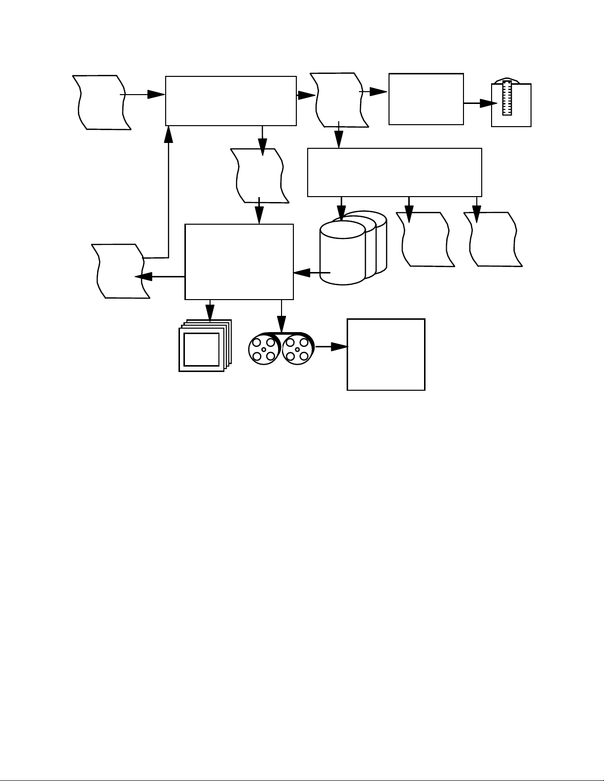
Front-End Script POEMS.CMD

POEMS Parameters File

foo.par

FIDO Input File

foo.par.in

FDTD Engine:

FIDO + CLUSTER SCRIPT

FIDO Log File

foo.par.err

FIDO

Output File

foo.par.out

FIDO

Field Files

POSTPROC Orders File

foo.orders

Postprocessor:

EMPOST.EXE

POSTPROC

RESULTS

foo.results

Optimization Loop

Image Files

Bitmap Image Files

CAD Export Utility

CAD File

Vis5D

Visualization Files

Vis5D.EXE

Visualization

System

or TEMPEST

Figure 2.1: POEMS system organization

2. HOW POEMS WORKS

2.1. Program Organization

The POEMS system consists of six parts: the front-end script (poems.cmd), which controls the whole process, communicating with the user, doing the less CPU-intensive tasks (such as CAD file generation) and controlling the rest; the FDTD simulation engine (FIDO or

TEMPEST), which takes a simulation description file and produces binary files of simulated

E and H field values; the postprocessor (EMPOST), which takes those huge binary files and produces secondary binary data and pictures, including VIS5D interactive visualizations; Vis5D itself, an open-source data visualization program running under the X Window system; and, optionally, a cluster control script (fidossh) that distributes parameters, starts the simulator instances, and collects data afterwards. We’ll examine these in turn.

2.2. The Front-End Script: poems.cmd

The front end script poems.cmd is the part of POEMS that the user will interact with (almost exclusively). It parses the input file, performs error checking, and handles all the symbols and equations. It generates the intermediate files that are used as input by

FIDO/TEMPEST and EMPOST, and produces log files and console output to keep the user

informed as to the progress of the run. The script is written in REXX, whose advanced parsing capabilities and very flexible stem processing made it a natural choice. Speed is not a serious issue, since only a tiny part of the run time is spent in the REXX code; almost all is used in the FDTD simulation.

2.2.1. Script Operation

The concept underlying the script’s design is that the user should be able to optimize or step anything he likes, in any combination. Therefore, user-defined functions, expressions, and variables are accepted anywhere an argument is required; as in a math program, these variables and functions can depend on each other in any fashion consistent with top-to-bottom parsing of the input file. This is straightforward in a single simulation run, but is a little more involved where stepping and optimization is being used: the program cannot make any assumptions about which simulation parameters can depend on the controlling variables. Accordingly, an optimization or stepping run is organized as follows.

a. Enter SETUP mode b. Parse the input file and set all the variables. Note which variables are to be stepped

or optimized (the controlling variables). c. Enter OPTIMIZE or STEP mode. For each iteration, (i)Update the controlling variables for the current iteration (ii) Parse the input file, setting all the variables except the controlling ones. This preserves all the dependencies. (iii) Generate the intermediate files for FIDO/TEMPEST and EMPOST, based on the current values of all the variables. (iv)Run FIDO/TEMPEST, capturing its console output to a file. (v)If FIDO/TEMPEST fails, stop. If it succeeds, call EMPOST to generate the inputs to the

merit function, plus any binary file, list, or slice bitmaps requested. Doing this on each iteration takes little time and helps in supervising the run’s progress. (vi)Based on the computed merit function, update the optimization simplex. If convergence has occurred, exit. Otherwise, compute new values of the controlling variables for the next iteration and keep iterating. If the current point is the best so far, save all the bitmap, list, and mode files under another name.

Of course, in order for this to do anything useful, you have to specify a merit function (or penalty function for pessimists) that depends on the simulation output.

2.3. The FDTD Engine: FIDO/TEMPEST

POEMS started out life using TEMPEST as its main component. TEMPEST is a more or less

vanilla single-processor FDTD engine, written originally for simulation of phase-shift masks, but quite widely used for a variety of applications. It is described in its own documents, which accompany the POEMS distribution. Due to the limitations of TEMPEST, in particular its lack of subgridding and multiprocessor capabilities, POEMS now relies principally on a specially written FDTD engine called FIDO, for FInite difference time DOmain. In broad outline, each of these programs parses an input file containing human-readable, hard-coded specifications of the simulation domain, boundaries, materials, objects, sources, and binary output files; constructs and runs a FDTD simulation as specified, stopping when the specified degree of convergence has been attained or the maximum cycles exceeded, and producing large binary files full of E and H values. TEMPEST comes with Matlab scripts to plot these simulated fields and do simple manipulations on them. Section A.2 has an example of a FIDO/TEMPEST input file generated by poems.cmd.

TEMPEST also has some more advanced capabilities, e.g. Fourier boundary conditions, far-

field computation (via the orders output command), and more complicated source shapes, that POEMS ignores in favour of its own more general versions. This was done for reasons of usability and to avoid being tied too tightly to one particular simulator engine. One additional (and most important) attribute of TEMPEST is that it is well validated. Besides having been tested on problems whose analytical solution is known, it has done a good job for lots of people over several years. For this reason, FIDO was written to be a plug-compatible superset of TEMPEST: it takes the same input files, and can do the same simulations, but FIDO is about 50% faster on a per-processor basis and can do subgridded and clusterized simulations as well. Thus in new situations we can test our simulations using TEMPEST and then refine them using FIDO.

2.4. The Postprocessor: EMPOST

Large binary files full of E and H values are not very useful by themselves. The tool set provided by POEMS requires a lot of CPU-intensive calculations and binary manipulations that are much better done in C++ than in REXX. Accordingly, POEMS uses a postprocessor written in C++ to do most of its numerical work. EMPOST takes a humanreadable but quite rigidly formatted orders file that specifies what is to be done on what data. An example is shown in Section A.3.

It is occasionally useful to run the postprocessor manually, e.g. when we want to change

from a linear to a logarithmic scale, change a colour palette, or something like that; simple changes like that are easily made directly to the generated file. EMPOST’s calling syntax is

empost orders_file results_file

The second argument is the name of a file that EMPOST produces, containing numerical results of the named orders, e.g. integrals, fluxes, mode matching coefficients, and so on. These are in the form of assignment statements, and are parsed by POEMS when postprocessing is completed. POEMS then uses these to compute the value of the penalty function for the current iteration.

2.5. The Visualization System: VIS5D

VIS5D is an advanced visualization program originally written for meteorological data. It runs under the X Window System, which is native to Linux and other Unix derivatives, but which has to be added to Windows and OS/2. Windows users can install Hummingbird Exceed, which works well with VIS5D once all the arcane X parameters are set up. See Appendix B for a working sample X configuration.

The Vis5D conversion code in empost is based on a stand-alone program by Theodore G. van Kessel. In this release, it is fully integrated into EMPOST. Both animated and static Vis5D files are generated using the MOVIE3D statement.

2.6. Cluster Control

There are lots of ways to structure a cluster, lots of communications styles (such as the Message Passing Interface (MPI), and lots of cluster management systems such as the Sun Grid Engine (SGE). POEMS is not tied to any of these, but is easily adapted to them. The main script runs on a frontend machine. Inter-host communication requires no specific support other than a high capacity, low latency TCP/IP network. FIDO uses TCP/IP socket communication between fido subdomains running on different hosts, and local communication between subdomains running on the same host. To allow the user control, cluster control is not hardcoded into POEMS, but relies on an external script. The supplied script is fidossh, which uses a shared file system (e.g. NFS, XFS, or PVFS2) for communication and ssh for cluster node control, This design is suitable for clusters of up to perhaps 20 nodes, depending on filesystem performance. The high bandwidth host-tohost communication is organized in a distributed fashion between cluster hosts, so the frontend machine does not become a bottleneck in small and medium sized clusters. For larger clusters, FIDO can use a hierarchical supervision scheme, where a single frontend node is not forced to supervise hundreds or thousands of hosts, but the cluster script would have to be tailored for the application.

The downside of this flexibility is that the user has to apportion the work manually. Future versions of POEMS will help automate this, based on the CPU speed, number of cores, and amount of memory possessed by each host. Probably it will remain semiautomatic unless the subdomains can be made very small.

2.6.1. Parallel Processing

[Under construction]

FIDO is a powerful and versatile simulation engine, which can compute simulations using

inhomogeneous cubic grids on uniprocessors, symmetric multiprocessors (SMPs), and clusters tied together with TCP/IP. From the POEMS user’s point of view, SMPs act just like uniprocessors, except that an N-way SMP needs its work divided up into at least N chunks, and the load balancing is manual--usually it’s easy. This section discusses multiprocessor operations; technical details are in Appendix C.

3. USING POEMS

Everything in POEMS is case-insensitive. Case is preserved but not significant in file names; specifying two names equal except for case will cause the first to be overwritten in Windows and OS/2 but not in Linux.

3.1. Command Reference

3.1.1. poems Command-Line Options

The calling syntax for POEMS is

poems parmfile <- option1 <option2 <option3>>>

where the options are one of DEBUG VERBOSE and RESTART. DEBUG prints lots of debugging information, VERBOSE prints more detail in the ordinary console output, and RESTART causes POEMS to parse the specified simplex file and restart the optimization run following the last completed iteration."

3.1.2. GLOBAL Group

ASSERT Syntax: ASSERT <expression>

Allows the user to add parameter error checking to the simulations. ASSERT functions very much like the assert() macro in C. Each time the input file is parsed (i.e. at the beginning of the run and before each iteration of the optimizer or stepper), <expression> is evaluated. If the result is zero, the run is stopped and a specific error message printed.

Example: ASSERT SourceZ ≤ Zsize-Tpml-lambda

COMMENT Syntax: COMMENT anything you want to say

Specifies a string that is to be included in all text and HTML output files. Useful for identifying information. You can use as many of these as you like. The output files will be more readable if you keep the total line length reasonable, e.g. 75 columns. Comment lines treat trailing commas as punctuation, not line continuation characters, so multi-line comments must be coded as a separate COMMENT statement for each comment line.

DEBUG Syntax: DEBUG on|off

Output lots of debugging information as the run proceeds. Useful mostly for the developer.

FREQ Syntax: FREQ <frequency in Hz> LAMBDA Syntax: LAMBDA <wavelength in metres>

Specify the frequency or free-space wavelength of the excitation sources (all will be the same). FREQ is an alternative to LAMBDA—use one or the other, but not both.

Examples:

FREQ 200*THz FREQ c/(1.464*700*nm) /* 700 nm in fused SiO2*/ LAMBDA 1.55*micron /* Communication wavelength */ LAMBDA 6.328e-7 /* He-Ne laser */

FUNCTION Define a user math function. User functions can be anything REXX

can evaluate, plus elementary functions (sin, cos, tan, asin, acos, atan, atan2, exp, ln), Bessel functions of the first kind of integer order (Jn(x)), complete elliptic integrals, and a few other odds and ends. Once defined, a user function can be used freely in expressions anywhere a literal number or a variable could. Functions may be defined in terms of variables, literals, or other functions, subject to the file parsing rules. When optimization is enabled, functions whose output values depend on variables being optimized over will have their definitions updated on each iteration to reflect the new values of these variables.

If the name of a formal parameter of the function is the same as that of a user variable, the formal parameter will override the user variable inside the function. Otherwise, any variables used by the function will be taken from the global scope. This allows functions to be parameterized by other variables, e.g. scale factors or offsets, which are not in the formal parameter list.

Syntax:

FUNCTION name(arg1, arg2,..., argN) = <expression>

Examples:

FUNCTION myfunc(a,x,q)=exp(a)*atan(q/x)*sqrt(23+q) FUNCTION parab(x,y,focus)=(x*x+y*y)/(4*focus) FUNCTION cone(x,y)=sqrt(parab(x,y,1)

HOSTS Specifies a file containing TCP/IP information on the hosts available

to run the current simulation.

Syntax: HOSTS <hostfile>

where entries in the given file are of the form

/* <optional_comment> <IP> <name> <port> <CPUs> <speed> <RAM MB> <Arch> <OS> e.g. for a Thinkpad T23 laptop,

/* Kukla--1.13 GHz PIII

127.0.0.1 localhost 1066 1 1.0 768 X86 OS/2 4.5

The port number is used for FIDO supervisory control, i.e. if this host is supervising N other hosts, those N connect to the supervisor using this port number. This port can be anything that doesn’t conflict with another service on the same cluster, but the unofficial "well-known" port for POEMS is 1066. All hosts can use the same port number.

NB: Hosts are identified by their hostname (as specified by the $HOSTNAME environment variable, rather than by IP address. This makes it possible to test cluster simulations on a single host by adding multiple names for the same host in the hostfile, and specifying different aliases in different SUBDOMAIN statements in the parameters file. Cluster script fidossl sets the HOSTNAME variable for each fido instance, which means that the host’s predefined hostname is not used.

MACDEF Define a user macro. Macros are parametrized groups of POEMS

statements, as opposed to functions, which compute numeric values. Macros are defined and expanded much like C preprocessor macros, except for the MACDEF and MACRO keywords. A macro definition must consist of a single logical line (i.e. if it spans more than one line in the source file, line continuation characters must be used to concatenate them into one logical line). Semicolons must be used to separate individual POEMS statements within the logical line. Both numeric and string values can be passed as macro parameters. Macros do not have local variables other than their pass parameters-

-other symbolic names will have their normal meaning from the local context at the time of macro expansion. Macro parameter names are dummy variables and will not collide with variables of the same name in the local context--context variables with the same name as the dummy will be inaccessible.

Macros are allowed to contain macros, i.e. the MACRO statement is permitted inside a MACDEF. (This is a powerful and dangerous feature.) Macro recursion is not supported. NB: Since POEMS comments always extend to the end of the current line, any comments inside a macro definition must be at the end of a lexical line, following the line continuation character, as shown below.

Syntax: MACDEF name(arg1, ..., argN) <logical line of code>

Example: This macro plots field files over a fixed volume, with a

given name and field component. The parameters xsize, ysize, zsize are not macro parameters, but will be supplied from the current context when the macro is expanded. Note the string concatenation used to generate the file names.

MACDEF FieldAll(kwd, fname)), /* Make I and Q field files

/* with appropriate file names and symbolic limits FIELD variable=kwd xlo=0 xhi=xmax ylo=0 yhi=ymax , zlo=0 zhi=zsize phase=0.0 state=steady file=fname’i’; , FIELD variable=kwd xlo=0 xhi=xsize ylo=0 yhi=ysize , zlo=0 zhi=zsize phase=2*atan(1) state=steady /* etc file=fname’q’;

MACRO Expand a user macro. Unlike MACDEF, which must be in the

GLOBAL group, MACRO can be used anywhere. Macro expansion is typographical, like C macros. String concatenation is performed, as shown in the previous example.

Syntax: MACRO name(arg1, ..., argN);

Example: Using the example from the MACDEF statement,

MACRO FieldAll(Ex, Ant01Ex);

is equivalent to

FIELD variable=Ex xlo=0 xhi=xsize ylo=0 yhi=ysize , zlo=0 zhi=zsize phase=0.0 state=steady file=Ant01Exi;, FIELD variable=Ex xlo=0 xhi=xsize ylo=0 yhi=ysize , zlo=0 zhi=zsize phase=2*atan(1) state=steady , file=Ant01Exq;

POSTPROCESSOR Tell POEMS which postprocessor executable to use (currently the

only choice available is empost).

Syntax: POSTPROCESSOR <postprocessor command line>

PRINT Print output, similar to the REXX SAY statement. Any number of

arguments may be supplied, and strings and expressions may occur in any order. Strings inside double quotes will be printed as is, whereas expressions will be evaluated first. PRINT statements are executed each time the input file is parsed, i.e. at the beginning of the run and before each tempest iteration.

Syntax: PRINT <"string"> <expression> ....

RANDOMSEED Supply a seed to the pseudorandom number generator.

Pseudorandom numbers are used only to choose starting points for the optimizer. The points visited by the optimizer for a given problem can be changed by choosing a different seed.

Syntax: RANDOMSEED <expression>

The value of <expression> must be in [0, 999,999,999], and its value is rounded to an integer before use. Thus values must round to different integers for them to be distinct for this purpose.

Example: RANDOMSEED 314159265

SET Defines a variable and sets its initial value. The expression may

contain literals, arithmetic and logical operators, predefined functions, and user functions.

Syntax: SET name = <expression>

Example: set hypot=sqrt(a*a+b*b)

SIMULATOR Give POEMS a simulator command line to use (no default). For

single-host simulations, this is just the simulator executable, but for clusters, it should consist of a command processor, script name, and any additional variables expected by the cluster script. To make this easier, POEMS defines two special variables, as follows.

Name Expands To $h Name of a file containing a list of all hosts actually used in

the simulation, one host per line

$f Name of a file containing a list of all files that need to be

distributed to the compute hosts for the current simulation.

POEMS constructs the command line by appending an at-sign (@)

and the name of a file containing the input parameters expected by

FIDO, then passes the resulting command line to the current shell.

The script blocks until the simulation returns.

Syntax: SIMULATOR <filename> [ <special variable> [<special variable> ]]

Example: SIMULATOR /usr/local/tempest/tempest

SIMULATOR rexx d:\poems\fido\fidossh.cmd $h $f

TITLE Give a title to the run. This title is printed in each file, and is also

used to generate names for the intermediate file and log file, and for the postprocessor orders file. No default.

Syntax: TITLE Waveguide3a

VERBOSE Turn on verbose output. Sometimes helpful in figuring out what’s

going on. It’s sufficiently verbose that it’s probably best to redirect it to a file or a pager program such as less.

Syntax: VERBOSE on | off

3.1.3. WORLD Group

BOUNDARY Sets boundary conditions for a given axis to be either periodic

(PERIODIC) or mirror-symmetrical (SYMMETRY). Only one need be set for each axis; if both are specified, they must be the same, since symmetry applies at both sides in FIDO/TEMPEST. (Deprecated boundary type ILLUM is the same as PERIODIC, and is provided for backward compatibility with earlier versions of POEMS.)

Parameters: xmin xmax ymin ymax zmin zmax Syntax: BOUNDARY <parameter> PERIODIC | SYMMETRY

SUBDOMAIN Defines a simulation domain. A domain is the portion of the

computational world assigned to one thread. Since the current version of tempest runs on a single processor, all domains will be joined together into one big tempest run. FIDO supports multithread simulations, so you don’t lose anything by putting them in. Parameter domain_name must not contain whitespace. For multiplehost simulations, the SUBDOMAIN keyword takes an optional hostname and base port number, indicating which host this subdomain is to run on, and the name of a supervisor host whose fido instance will control that host. If these parameters are not supplied, the given subdomain runs on the local host. (The supervisor parameter should not be supplied for the host in overall control.) All subdomains running on a given machine must specify the same supervisor, or a runtime error will result. Each

subdomain uses 6 sockets, attached to port, port+1,..., port+5, all of which must be unique on the given host, though there is nothing to stop different hosts from using the same port numbers. Port numbers must be between 0 and 65535, and it is usually best to use numbers greater than 16384.

Syntax: SUBDOMAIN <domain_name> [host=<host> port=<port> ,

super=<super>]

BASICSTEP Specify the size of the cubical cells that make up the current

subdomain. SI units are suggested, because the scaling between E and H used internally assumes SI units. From POEMS’s point of view, this number isn’t necessarily set in stone: the step size, time step, and domain size can all be controlled by the optimizer or the stepper if desired. For future use, keywords XBASICSTEP, YBASICSTEP, and ZBASICSTEP are also allowed, but since in this release the cells must be cubical, only one of the four may be specified.

Syntax: BASICSTEP <expression>

Examples: BASICSTEP lambda/20.5

BASICSTEP 0.1*micron

XRANGE YRANGE ZRANGE Sets the X, Y, or Z limits of the current domain. The parameters

must obey max_expression > min_expression ≥ 0.0.

Syntax: XRANGE <min_expression> <max_expression>

3.1.4. MATERIAL Group

DEFINE Defines the parameters of a material to POEMS.

Parameters: matname type epsReal epsImag muReal muImag n k conductivity Types: dielectric metal PML conductor PEC black magnetic

Type dielectric

Ordinary nonmagnetic material, with n ≥ k. Most optical

materials are of this type: vacuum, air, glass, and plastics.

Parameters: n, k (real and imaginary refractive index) Example:

DEFINE matname= BlackGlass type=dielectric n=1.52 k=1e-3

Type metal

Nonmagnetic dispersive material which may have negative dielectric constant at the frequency of interest, which is equivalent to having n < k, e.g. metals in the infrared. Other conductive materials can be modelled as conductor type. There are two ways of specifying a metal: using the n and k values at the centre wavelength of the sources, or using a file produced FITMAT, which fits Debye and Lorentz poles to user-supplied n,k data.

Parameters: n, k , file Example:

DEFINE matname= Gold3_1um type=metal n=0.3 k=11.23 DEFINE matname= Nickel type=metal file=nickel.poles

Type conductor

Normal conductor, with ε = ε0+jσ/ω Useful for metal

waveguide boundaries, at frequencies where the normal conduction model applies (below about 1 THz). In optical simulations, ordinary conductors are primarily useful in simulating loads.

Parameters: conductivity (in units of (Ωm)-1)

Example:

DEFINE matname=copper type=conductor conductivity=5.8e7

Type magnetic

Magnetic material, whose properties are specified by

complex µ and ε, specified in SI units, not the relative µ and ε.

Parameters: epsReal epsImag muReal muImag

Example:

DEFINE name=ferrite type=magnetic epsReal=18,

epsImag=0 muReal=220 muImag=1.1

Type PEC Type black

Perfect conductor. All fields inside a PEC are zero. Sometimes useful for saving CPU cycles in regions where the fields are known to be zero, e.g. deep inside metal objects.

Parameters: none

3.1.5. OBJECT Group

Like all dimensions in POEMS, object dimensions are measured from edge to edge, as you would measure with calipers. All dimensions are correctly rounded to the nearest multiple of basicstep in the subdomain in which they occur. A cell is included if its centre lies inside the specified region. This can lead to steps at boundaries between subdomains with different basicstep values, due to differences in rounding.

When an object’s midline is specified in terms of a curve, e.g. FAN, GRATING, CURVE, and 3DCURVE, the end points of the curve are taken to lie at the centre of the outermost plane of blocks on each end. This makes sure that if the local object axis is highly inclined, the outermost blocks don’t disappear due to their centres falling outside the region, as they would if the endpoint were taken to lie in the outer face. Sufficiently inclined objects may still become discontinuous.

BLOCK Adds a rectangular prism (like a shoe box) of material matname,

covering the region xlo ≤ x ≤ xhi, ylo ≤ y ≤ yhi, zlo ≤ z ≤ zhi. Like

everything else in POEMS, these dimensions will be rounded to the nearest cell boundaries.

Parameters: matname xlo xhi ylo yhi zlo zhi Example:

block matname = AirPML xlo=0 xhi=8*dx ylo = 0 yhi=ymax ,

FAN Adds a fan shaped object such as a dielectric waveguide horn or

taper. A fan is specified by a choice of curve and rectangular end faces 1 and 2, defined by their diagonal points ((xlo1,ylo1,zlo1), (xhi1,yhi1,zhi1)) and ((xlo2,ylo2,zlo2), (xhi2,yhi2,zhi2)). These must be parallel and lie in a coordinate plane. Intervening planes are defined by the choice of taper and the taper parameter, which is a scale factor for the domain of the curve—increasing the parameter causes the taper to be sharper, and decreasing it makes the taper more gradual. Allowed tapers are LINEAR, EXPONENTIAL, and ERF. Exponential tapers are useful for converting guided waves to free space, and ERF tapers are useful for converting between different-sized waveguides without strong back reflections from either end.

zlo=0 zhi=zmax

If the two end faces are the same size and shape, all the curve shapes are equivalent. The end faces can be offset laterally, so that a fan statement can build a diagonal line.

Parameters: matname taper taperpar xlo1 xhi1 ylo1 yhi1 zlo1 zhi1 xlo2

xhi2 ylo2 yhi2 zlo2 zhi2

GRATING Adds a planar grating with lines of rectangular cross-section. The

line width and phase of the grating are arbitrary, and specified with user functions of the coordinate variables. Thus the grating can have its properties altered in a very general way during optimization, e.g. having its Seidel aberration coefficients controlled to optimize a coupling efficiency. Gratings are implemented by evaluating phasefunc at a grid of points in the plane, and constructing a phase contour map. Each grating line is generated

by following the contours at integral multiples of 2π, and centring a

rectangular block of total width defined by widthfunc on the contour line, so that the grating’s diffractive strength is also a function of position. Making the width too large or too small will result in the spaces or lines disappearing, which is one way of making a grating with a non-rectangular boundary. The default spacing between phase points is two cells, but this can cause the script to run very slowly, so it can be overridden with the optional parameter interval. The interval parameter determines the grid on which the phase and width functions are sampled, which influences the accuracy of the contour maps and hence the grating placement.

Parameters: matname orientation xlo xhi ylo yhi zlo zhi widthfunc

phasefunc [interval]

HOLLOWBOX Adds a hollow box (rectangular shell) of specified outer dimensions

and thickness. It is implemented by dividing up the rectangular box into 26 smaller blocks: 6 for the faces, 12 for the edges, and 8 for the corners. This primitive is especially useful for using PMLs to isolate a region from its surroundings. When used with PMLs, the outer dimensions must be the same as those of the simulation domain. The PML absorption directions will be the outward normals for the flat faces, outward-directed face diagonals for the edges, and outward-directed body diagonals for the corners.

Parameters: mattype xlo xhi ylo yhi zlo zhi thickness

TILEDPLANE Adds a tiled plane (thick rectangular sheet) of specified outer

dimensions. It is implemented by dividing up the rectangular sheet into 9 smaller blocks: 1 for the face, 4 for the edges, and 4 for the

corners. This primitive is especially useful with plane wave illumination, where we want PMLs only on the front and back faces of the region. The wide face of the object must touch one of the faces of the simulation domain. The PML absorption directions will be the outward normals for the face, outward-directed face diagonals for the edges, and outward-directed body diagonals for the corners. If for some reason you call this with an ordinary material, it just adds a regular block.

Parameters: mattype xlo xhi ylo yhi zlo zhi

CURVE Adds a curved object whose path is expressed by a user-defined

planar curve, (u(s), v(s)), and whose outline is swept out by the region f(q,r) > 0 as the parameter s advances from slo to shi. Variable q is the normal to the plane, and r is parallel to q × (du/ds, dv/ds). This statement can be used to make very general curved objects of variable cross-section. Due to the uniform rectangular grid employed by FIDO/TEMPEST, curved objects will look somewhat different depending on the direction of their axes at any given place. POEMS attempts to minimize this effect.

Parameters: mattype slo shi perp hfunc vfunc

Not implemented in this release.

3DCURVE Like CURVE, but the axial curve is allowed to be nonplanar. This

statement is more complicated to use, due to the noncommuting property of 3-D rotations—in specifying the functions u, v, w, it’s easy to get mixed up by the way they rotate around.

Parameters:

Not implemented in this release.

CYLINDER Adds an object whose axis is a straight line, but whose outline is an

arbitrary function of the perpendicular coordinate.

Parameters: mattype axis lo hi maxradius insidefunc

Not implemented in this release.

3.1.6. SOURCE Group

GAUSSIAN Produces a TEM00 Gaussian beam, centred at (x, y, z), with 1/e

diameter width, whose axis is specified by the vector(kx, ky, kz), which can have any length. The E field is linearly polarized, with components (mag*Ex, mag*Ey, mag*Ez). Circular or elliptical polarizations can be synthesized by using two with different phases. In this release, orientation must be XY, because tempest can’t handle plane waves whose source locus isn’t perpendicular to z. Also in this release, the focus of the beam is at the plane of excitation, i.e. xfocus, yfocus, and zfocus don’t do anything yet. This will be fixed in the next release.

Parameters: x y z width kx ky kz Ex Ey Ez mag phase n k orientation

AIRY Similar to Gaussian, but with a uniform pupil function, giving rise

to an Airy pattern (J1(x)/x) at the focus.

Parameters:Not implemented in this release.

PUPILFUNCTION Similar to GAUSSIAN, but allowing a general user function f(u,v) to

be used as the pupil function. GAUSSIAN is already implemented on top of this function, but it hasn’t been exposed for this release.

Parameters:Not implemented in this release.

PLANE Adds a linearly polarized plane wave source. The position

parameters x, y, z specify the point at which the plane wave has the given phase.

Parameters: x y z kx ky kz Ex Ey Ez mag phase orientation

MODEFILE Adds a mode file source. Mode files are lists of E field components

vs position, produced by the MODEFILE output statement in a previous POEMS run, allowing the output of one run to become the input of another. This is especially useful in waveguide problems such as the one in Section 3.6.3. The coordinates specified are the centre of the mode array, which is in general offset from the origin.

Parameters: file x y z orientation

POINT Adds a linearly-polarized point electric dipole source at the given

position. Point sources whose polarization is not x, y, or z (diagonally, circularly, or elliptically polarized) can be implemented as two or three point sources with appropriately chosen magnitude and phase.

Parameters: x y z Ex Ey Ez mag phase

3.1.7. COMMAND Group

COMPUTE Supply control parameters to FIDO/TEMPEST. Parameters mincycles

and maxcycles control the number of cycles of the excitation frequency that each simulation may use; setting the lower limit occasionally helps in avoiding spurious early convergence, and the upper puts a bound on the amount of run time. Adjusting maxcycles to a small number such as 1-3 is useful when setting up a run, because you can get rapid feedback on whether your geometry is correct, and whether your PMLs are likely to cause problems. Slightly higher values are useful in the early stages of an optimization, where extreme accuracy in penalty function evaluation is not needed, but run time is a serious concern. See the TEMPEST documentation for more details. Start with a value of 0.01 or 0.001 for reltolerance, and don’t set mincycles or timestep until you really need to.

Parameters: reltolerance maxcycles mincycles timestep

3.1.8. OUTPUT Group

INDEXN Tells tempest to produce a field file containing the real part of the

refractive index at each point. This is useful to show which material is where in the simulation domain.

Parameters: xlo xhi ylo yhi zlo zhi file

DECIMATE Specify that only 1 out of decimation points is to be kept in each axis.

Parameters: xdecimation ydecimation zdecimation

Not implemented in this release.

FIELD Tells tempest to produce a field file containing the specified field

variable at each point.

Parameters: variable xlo xhi ylo yhi zlo zhi x y z file

phase state

3.1.9. POSTPROCESS Group

CAD Produces a .ctxt (2-D) or 2-D or 3-D DXF file of the entire

simulation domain, suitable for importation into a CAD program, e.g. for numerically controlled machining, photomask generation, or documentation. In a 3-D DXF file, each block in the simulation domain becomes a set of six 3DFACE entities. In a .ctxt or 2-D DXF file, each block is projected onto two rectangles, representing the upper and lower faces in the given orientation. POEMS DXF files are known to import properly into several CAD packages including Autodesk Inventor. Note that length unit used in the DXF file is metres unless otherwise specified--since many CAD packages use a fixed number of decimals, this may cause confusion when the sample domain is very small (e.g. in optical waveguides). Note that the orientation is ignored in a 3-D file.

Parameters: file filetype dimensions orientation units xcut ycut zcut space

Examples: CAD file=ofile3.dxf filetype=dxf dimensions=3

CAD file=ofile2.dxf filetype=dxf dimensions=2, units=micron orientation=ZX CAD file=ofile.ctxt filetype=ctxt units=micron, orientation=XY

The CAD statement also permits defining a line (for 2-D) or a plane (3-D), parallel to a coordinate axis, at which extra space is to be inserted, for use with shadow mask fabrication. For instance, for a bridge width of 1.5 µm, you can add the following to the CAD statement:

CAD file=mask.ctxt filetype=ctxt units=micron orientation=XY, xcut=1.8*um space=1.5*um

WEBPAGE Produces a static HTML page containing all the relevant run

parameters, output bitmaps, and links to other files such as DXF and Vis5D.

Parameters: file

FARFIELD Computes the far-field limit of the fields at a given plane, specified

as xlo ≤ x ≤ xhi, ylo ≤ y ≤ yhi, zlo ≤ z ≤ zhi. Because this range must

specify a plane, the upper and lower limits of one axis must be the same to within basicstep/2. The coordinates will be correctly rounded to integral numbers of cells. We assume that the fields propagate through an infinite half-space of refractive index n (which obviously must be lossless). The refractive index is taken to be the real part of the index in the actual model at the centre of the

supplied plane, {xmin ≤ x ≤ xmax, ymin ≤ y≤ ymax, zmin ≤ z ≤ zmax}.

The parameter direction can be up or down depending on which direction we’re interested in. Internally, POEMS uses both E and H field information to separate out the incoming and outgoing fields, so the computed far field spectrum wht direction=down can be very different from that with direction=up. At present this statement produces bitmaps of s- and p-polarized field amplitude and phase at each point (u, v) in the pupil plane.

Currently the FARFIELD statement can be applied only on planes of uniform granularity, i.e. basicstep must be the same in all subdomains cut by the given plane.

Parameters: name xlo xhi ylo yhi zlo zhi file direction

FLUX Computes an integral of the Poynting vector through the given

surface, in the inward direction. This isn’t quite the same as using the INTEGRAL statement directly, because it adds the ability to specify an interior point. A positive flux is going in the direction towards from (xInside, yInside, zInside).

Parameters: name xinside yinside zinside xlo xhi ylo yhi zlo zhi

INTEGRAL Computes a volume or surface integral of a given field function by

summing all the blocks lying in the specified region. If the region has a nonzero thickness (after rounding to the nearest multiple of BASICSTEP), it’s normalized as a volume integral; if two have a nonzero thickness, it’s normalized as a surface integral of the broad face of the region; and if only one dimension has a nonzero size, it’s normalized as a line integral. Specify the integrand field or postprocess quantity as variable, and make sure there’s a matching statement that generates an array of the given quantity, because it won’t be done automatically.

Parameters: name variable xlo xhi ylo yhi zlo zhi

LIST Stores a list of field values as ASCII floating point numbers, suitable

for reading into a spreadsheet or a plotting program such as GNUPLOT. The row-column arrangement of a 3-dimensional list file depends on the value of orientation. Coordinate axes are always taken in cyclic order, with the leftmost position in the first line corresponding to the minimum of all coordinates; in a 2-D list in XY orientation (perpendicular to Z), columns correspond to the x coordinate and rows to the y coordinate. In YZ orientation, y goes across columns and z goes down rows, and in ZX orientation, z goes across columns and x down rows. (ZY is the same as YZ, and XZ is the same as ZX--cyclic order is always preserved.) In a threedimensional list, the perpendicular variable is most slowly varying. For example, in XY orientation, a 3-D list file with M planes (Z) N rows (Y) and P columns (X) would have list N rows for the first plane, another N for the second plane, and so on. The file format is as follows, with integer indices i, j, and k corresponding to coordinates x, y, and z.

Parameters: variable file orientation xlo xhi ylo yhi zlo zhi phase indexn

kmin kmax jmin jmax imin imax lambda indexN dz dy dx coordinates arrangement

(real, imag) (real, imag) (real, imag)....

...

(real, imag) (real, imag) (real, imag)....

The value of coordinates can be polar or rectangular, and arrangement can be normal or FFT.

MODEFILE A variation on the LIST command, for producing 2-D list files of Ex,

Ey, and EzThe appropriate file name additions are supplied

automatically. Parameters: file orientation xlo xhi ylo yhi zlo zhi phase indexn

MODEMATCH Computes the far-field pattern of the simulated fields, taken from

the given plane, and compares it with the analytically computed pupil function requested. It returns the normalized overlap integral of the two across the (u, v) plane. This is a complicated way of saying that MODEMATCH returns the coupling efficiency from the simulated plane to a receiver whose sensitivity pattern matches the given pupil function, e.g. a fibre. Known pupil functions at present are GAUSSIAN, AIRY, FLATTOP, and BESSJ0. The refractive index is taken to be the real part of the index at the centre of the given plane, as in the FARFIELD order.

Parameters: name xinside yinside zinside function exi exq eyi eyq ezi ezq

xlo xhi ylo yhi zlo zhi xfocus yfocus zfocus xNA yNA zNA NA direction

MOVIE Produces an animated one-cycle GIF of N frames, over the given

plane. Parameters:file orientation xlo xhi ylo yhi zlo zhi dt frames variable

Not implemented in this release.

MOVIE3D Produces an interactive Vis5D animation of up to 9 field variables.

Setting frames=1 (the default) produces an instantaneous snapshot, which you can explore interactively, which is most suitable for timeaveraged and time-independent quantities such as refractive index and power dissipation density. To see the complex-valued fields change, set frames to a positive integer N. This produces an Nframe 3-D animation covering one cycle of the excitation, the i

frame corresponding to a phase of i/N (counting from zero).

Due to a limitation of VIS5D, the size of the space cannot exceed 100 cells in each direction. If you call for a region larger than this, it will be decimated automatically by the smallest integer factor that allows it to fit into 100 pixels. Up to 100 frames of animation may be specified, and any POEMS variables are allowed. There is no provision for setting phase angles, as the animation will cover a full cycle.

Parameters: frames variable1 variable2 variable3 variable4 variable5

variable6 variable7 variable8 variable9 xlo xhi ylo yhi zlo zhi file

AMPLEX, AMPLEY AMPLEZ, AMPLHX AMPLHY, AMPLHZ PHASEEX, PHASEEY PHASEEZ, PHASEHX PHASEHY, PHASEHZ POYNTINGX, POYNTINGY POYNTINGZ These statements compute the amplitude and phase of E and H

fields, and the time-averaged Poynting vector. The output is a tempest-style field file suitable for further processing. In the current release, each field component desired must be specified manually before anything else is done to it, because otherwise the array won’t exist when it’s needed. There’s a wish list item to make the postprocessor smarter about file handling and memory utilization. Parameters: xlo xhi ylo yhi zlo zhi x y z file

DISSIPATION Power dissipation density , -∇ S (the Poynting vector). Normalized

to the volume of one cell, so that volume integrals of this quantity give the correct power dissipation inside the region. Parameters: name xlo xhi ylo yhi zlo zhi file xinside yinside zinside

SLICE Produce a bitmap of variable over the given domain, with control

over the colour palette and the scale. Variables are always taken in cyclic order, i.e. x, y, z, x, y, z,..., which preserves the righthandedness of the coordinate system. The positive sense of the perpendicular axis is always out of the screen towards the viewer. (Technical detail: The Windows bitmap format has the pixel index starting at (0, 0) in the upper left corner of the screen, so that the column index corresponds to position correctly but the row index is inverted. POEMS flips the row index internally, so that the screen coordinates are correct for the simulation geometry--positive X is to the right, positive Y is up.)

Perpendicular

Z XY X Y Z

X YZ Y Z X

Y ZX Z X Y

Table 1: Axis orientations for SLICE bitmaps

Orientation

Increasing to right

Parameters: orientation variable phase xlo xhi ylo yhi zlo zhi file curve

palette palfile

Choices of palette are grey, saturation, flame, bluered, and custom. Grey scale palettes are simple and unexciting, but clear. Saturation palettes keep the luminance level nearly constant (except that value 0 is black), but vary the hue from yellow to a saturated blue. Flame palettes start out black, go through dark grey, dull red, bright red, orange, yellow, white, and blue-white, mimicking the colour of a hot object. The bluered palette is suitable for bipolar values such as E and H fields; it forces white to be at value 0, with increasing red saturation for positive values and increasing blue saturation for negative values. A custom palette requires a palette file palfile. These are text files with the form

level R G B<newline> level R G B<newline> ...

Increasing upwards

Increasing out of the screen

where level, R, G, and B are integers between 0 and 255, inclusive. The level column represents the signal level, and R, G, and B are the usual RGB colour components.

Choices of curve are linear, gamma, logarithmic, and MuLaw. The linear curve spaces the palette entries out evenly, with the maximum value in the picture being 255 and the minimum, 0. The gamma curve first takes the square root of the absolute value of the variable, restores the sign, and spaces out the result evenly. This accentuates details in the weaker-field regions, without losing definition in the higher-field regions. The logarithmic curve accentuates weak fields very strongly, which is very useful in some cases but tends to lose detail where the field is strong. The mathematical logarithm is modified to avoid floating-point runtime errors: it actually computes

where x has been normalized by the largest element in absolute value. The MuLaw curve uses the CCITT µ-255 codec curve, which is linear for values near the positive and negative limits, but puts the levels close together near zero. While this resembles a bipolar version of the logarithmic curve, it actually combines many of the advantages of the linear and logarithmic curves, since not all detail is lost at the highest values.

Syntax: SLICE file = <fname> xlo=<value> xhi=<value> , ylo=<value> yhi=<value> zlo=<value> zhi=<value> , phase=<value> variable = Ex

Example:

SLICE file = /var/tmp/v1aExIsourceZ.bmp xlo=0 xhi=xsize , ylo=0 yhi=ysize zlo=1.5*um zhi=1.5*um phase=0 , variable = Ex

3.1.10. OPTIMIZE Group

VARIABLES Tell the optimizer which variables to optimize over. These must

have been defined in a SET statement. Syntax: VARIABLES var1 ... varN

GUESS Supplies a guess to the optimizer. A guess is a point in the N-

dimensional parameter space. For an N-dimensional optimization run, N+1 guesses are required, each supplying all N variable values. The first guess is supplied by the SET statements where the optimization variables are defined, but additional ones can be supplied by GUESS statements. If more than N+1 guesses are

supplied, guess N+2 overwrites guess 1, and so on. You can supply a pre-computed value for the penalty or merit function, by including

merit=<expression> or penalty=<expression>

in the GUESS statement. While this can save valuable time, it must be used with care, because POEMS will trust the value you give it. If the value is stale or otherwise incorrect, this will interfere with the optimization. If the supplied value is unrealistically poor, the optimizer will incorrectly tend to move away from it, good, whereas if it is too good, the optimizer may get stuck in that vicinity, trying to improve a value that is better than any available computed value.

Syntax: GUESS <var1> = <expression> <var2> =, <expression>....

[penalty = <expression>]

LIMIT Expression that has to be true for a valid point. Often it’s better to

change the simulation parameters to build the limits in--e.g. replacing width with abs(width) or using more complicated functions of absolute values. LIMIT is better for more complicated functions, e.g. forcing the corners of some structure to lie within an arbitrary boundary. Not implemented in this release. Syntax: LIMIT <Boolean expression>

Example: LIMIT length*width*height ≤ MaxVolume

STORE Specify a file to store the simplex for each iteration, along with the

corresponding penalty function values. These are in the right format to be cut and pasted back into the parameters file to restart an interation without losing previous work. Syntax: STORE <filename>

PENALTY MERIT Defines an expression on which the optimizer is to work. Merit

functions are maximized, and penalty functions are minimized. Only one of the two can be specified. In order for the optimizer to do anything useful, the optimization expression must depend on each of the optimization variables. Note that any variable

assignment involving quantities computed by the postprocessor will not be updated at postprocessing time. That means that the

dependence on this iteration’s results must be included explicitly in <expression>. For example, if the iteration is minimizing the loss of a coupler, you might specify MERIT 10*log10(efficiency), which will work fine, but you can’t use SET dBloss=-

10*log10(efficiency) up in the GLOBAL section and then specify PENALTY dBloss in the OPTIMIZE section--if you do, you’ll wind

up with stale data. This can sometimes be useful, but not usually.

Syntax: MERIT <expression> OR PENALTY <expression> Example: PENALTY 100*(OutputFlux/InputFlux - 1)

PARAMETERS Defines quantities to guide the optimizer. The number of function

evaluations (i.e., tempest runs) per restart will not exceed iterations, convergence will be declared when the penalty function value in all the simplex points is within tolerance of the best value, and the optimizer will be restarted restarts times after converging or running out of iterations.

Parameters: iterations tolerance restarts Example:

PARAMETERS iterations=35 tolerance = 1e-3 restarts = 2

3.1.11. SCHEDULE Group

Stepping is not implemented in this release.

VARIABLES Tell the stepper which variables to step. These must have been

defined in a SET statement.

Syntax: VARIABLES var1 ... varN

RANGE Tell the stepper how far, and at what intervals, to step variable

varname.

Parameters: varname lo hi stepsize

STORE Supply a file name for the stepper’s results.

Syntax: STORE <filename>

3.2. The Computational Domain

1 2 3 4

0 1 2 3 4 5 6 7 8

Image Domain

Actual Domain

Next Period

N rows

N-2 Rows

Unfolded

2N-2 Rows

3.2.1. Symmetry

Many technologically useful devices have a periodic structure. The periodic boundary conditions assumed by POEMS are a natural fit to such structures, which can be simulated very efficiently. This happens automatically if you leave out the absorbers on the sides facing the periodic direction. Almost as many devices exhibit symmetry planes. A domain with a symmetry plane, illuminated symmetrically, will exhibit completely symmetric fields, so no extra information is generated by simulating both halves. Splitting the domain in half down the symmetry boundary can save half the run time and half the memory, while preserving the same level of detail in the results. Domains with more than one symmetry boundary save even more (though this begins to restrict the illumination more severely). POEMS (via support built into TEMPEST, FIDO, and EMPOST) supports symmetrical simulations.

It’s important to visualize the symmetry arrangement correctly, and it isn’t what one might first think: A symmetry plane actually slices right through the centre of the outermost elements. Say the X axis has 100 cells, numbered 0-99. Normally, periodic boundary conditions apply, and cell 0’s neighbours are 1 and 99. If X is a symmetry direction, cell 0’s neighbour is cell 1 on both sides. That is, a 1-block wide layer lying against the symmetry axis has the same effect as a 1-block layer in the middle of the unfolded domain. A 2-block layer against the symmetry axis is equivalent to a 3-block layer down the middle of the unfolded domain.

Figure 2.2 Geometry of a symmetry boundary with N=5

Another way of stating this is that if a symmetry plane is like a mirror, then we’d expect that a block pushed right up against it would look like two blocks. With POEMS, we have to think of it as pushing a block up to and halfway through the mirror, so it still looks like one block. A one-block layer at the symmetry axis unfolds to one block, a two-block layer unfolds to three blocks, and in general N blocks unfold to 2N-1 blocks. Furthermore, you can’t have symmetry just on one side--if X is a symmetry direction, both the xmin and xmax faces are symmetry planes.

We’re typically using symmetry to improve the tradeoff between the block size and the number of blocks required-in other words, trying to get the finest level of detail we can afford. Implementing symmetry the other way, so that a one-block layer at the symmetry axis unfolds to 2 blocks, means that there is no way to get 1-block details at the symmetry axis. At least one symmetry plane is usually right in the middle of the region of interest, so this reduces the value of symmetry in saving computation. Thus this seemingly odd choice is in fact superior. However, it does have significant consequences for postprocessing, e.g. you can’t just compute the flux over half the area and double it, because that will count the blocks on the symmetry axis twice. The postprocessor code handles this by halving the weights of blocks lying against the symmetry axis. The halving happens separately for each axis, so that if there are two symmetry directions, the symmetry face blocks have weight 0.5 and the ones down the intersections of the symmetry planes have weight 0.25. Thus the integrals and fluxes computed by POEMS can be simply multiplied by a factor of 2 per symmetry axis to yield the correct result for the unfolded domain.

We commonly want to run a symmetric simulation once in the full domain and once in the halved or quartered domain, to make sure everything comes out the same. To do this in POEMS, remember that if the folded dimension has N cells, its invisible other side has N-2 cells. (The end cells are special.) Thus the full domain will be 2N-2 cells wide. If you run the full domain first, you must give it an even number of cells in the symmetry direction.

Symmetrical domains of course must have symmetrical illumination. The TEMPEST approach is to forbid such domains to have off-axis plane waves applied to them. The other approach would have been to double each plane wave source, so that their result was symmetric, which would be preferable. Since the xxBEAM source statements are implemented as sums of plane waves, we can’t use them on symmetric domains. Use mode sources instead. It isn’t difficult to make a mode source out of a beam source: just run a three-cycle simulation of the desired beam shining into an empty domain, and make the mode file in a plane near the source.

3.3. OBJECTS

Everything in the simulation domain is made up of cubical blocks arranged in a simple cubic lattice, so there’s a limit to how subtle we can be in specifying curves and angles. Nonetheless, POEMS provides a wide array of object types that can be parameterized in powerful ways, as discussed in the command reference.

3.3.1. Perfectly-Matched Layers

PMLs are fictitious anisotropic materials that (usually) absorb whatever radiation falls on them from pre-specified directions. They work extremely well when they work at all, which isn’t 100% of the time.

PMLs don’t absorb in every direction, so different parts of the domain need different PMLs. This is such a pain that POEMS makes a valiant effort to automate it for you. It works as follows:

(i)If a PML touches a boundary, it will be set to absorb energy falling on that boundary from the centre of the domain. (ii)If a PML touches more than one boundary, rule(i) will be applied to all of them. (iii)PMLs that touch both the upper and lower boundary of an axis will be automatically split in half down the middle so that (ii) can be applied to both halves. (iv)PMLs must touch at least one boundary.

A solid block of PML filling the whole space is thus split into 8 blocks, each absorbing diagonally outwards. You can manipulate these rules to customize PMLs for your use. One common desire is to have PMLs covering the whole outer skin of the domain, with the faces, edges, and vertices all absorbing in different directions (26 blocks altogether). This is fiddly, so the HOLLOWBOX statement was added to POEMS to take care of it. HOLLOWBOX is implemented by splitting the box up and letting the automatic PML handler apply rules (i)-(iv) to each block. The TILEDPLANE statement does the same for planar PML regions.

POEMS has heuristics for generating reasonable PMLs automatically, but these are not

always reliable. Signs of trouble are checkerboard patterns, fields apparently originating in PML regions, floating-point runtime errors, and the generation of NaNs. This will happen every time if you put a material boundary near a PML, or if you have sources inside it. A reasonably safe rule is to put a PML no closer than 1 wavelength from a material boundary or a source. Plane waves and PMLs are a difficult combination in

TEMPEST.

3.4. MATERIALS

Materials used in POEMS are treated as isotropic, linear and time-invariant. tempest supports photoresist materials and has limited support for anistotropic ones, so if this becomes important it can be added in a future release.

3.5. SOURCES

POEMS has a rich array of sources, and when the PUPILFUNCTION order becomes

available, it will be able to generate essentially any monochromatic propagating field.

3.5.1. POINT SOURCES

In continuous-space electrodynamics, static point sources are mathematically very simple. In electrodynamics, there are no monopole sources, since a monopole field is purely radial, whereas electromagnetic waves are purely transverse. The simplest physical

source is therefore an oscillating dipole. FDTD codes model a dipole as a single-cell source whose E field oscillates in time, just as you’d expect. Unfortunately, only linearlypolarized sources are supported because only a single point source can occupy a cell. This restriction is not essential, and may be removed in a future release.

The other problematical thing about point sources is normalization. One might expect that a point source of strength 1 would produce an E field at the source of 1, but that isn’t how TEMPEST’s point sources are normalized. This and other normalization problems (of which there are a few) will be fixed in a future release. The problem doesn’t affect power ratios and efficiencies, which is what we usually care about.

Figure 2.3 TEMPEST divergence due to source inside PML. This box is 3.2 wavelengths across.

Figure 2.4: Side view of the domain of Figure 2.3.

3.5.2. PLANE WAVES

Because of the periodic boundary conditions assumed in the simulation geometry, POEMS has a lot in common with FFT programs, e.g. point N is the same as point 0, and only waves whose spatial frequencies are integral multiples of 1/(N dx) can be used. Since dx

<< λ, and memory is limited, in practice only a few dozen or at most a few hundred

plane wave components are necessary to synthesize any desired pupil function. The down side is that the resulting beams are spatially periodic, and their side lobes will leak into adjacent domains.

A plane wave source produces radiation in only one direction, and does not interfere with other field components crossing it. Plane waves don’t work well with fully isolated domains, i.e. those with PMLs on all surfaces. It’s useful to put PML boundaries downstream of the illumination, but when using plane waves, some imaginary absorbing material boundary is often better behind the illumination surface.

FDTD codes use periodic boundary conditions. Fields leaving through one side will magically reappear coming from the other, which may lead to divergences if you don’t put in absorbers of some sort. Sloppy absorber design may lead to fields travelling many, many periods, leading to anomalously slow convergence. Figure 2.4 is an example of a divergence due to PMLs used with plane wave sources. Note that the divergence looks electrostatic—the wavelength is far too short to propagate. This is a good clue that something is wrong.

Figure 2.5: 120-µm long doped silica waveguide, excited with a circular Gaussian beam of diameter equal to its core width. A black glass region is at each end (waveguide1c.par).

Figure 2.6 Detail of the launch end. Note the unidirectional character of the Gaussian beam source, and the weak reflected field leaking back through the illumination plane after travelling about 110 µm.

Figure 2.7: Mode source for a 5-µm doped-silica

waveguide (∆n=0.02). This slice is taken at the

plane of the sources, showing the strong nonuniformity.

3.5.3. BEAM SOURCES

Beam sources are made up of sums of plane waves. They share the unidirectional property of plane sources. This is sometimes useful in waveguide simulations, because you can bounce the wave off a mirror at the far end and look at the field coming backwards through the plane wave surface. Since all of this field has travelled twice the length of the waveguide, it can make a good approximation of the waveguide mode. This is where the mode file used in 3.5.4 came from.

3.5.4. MODEFILE SOURCES

Modefile sources are actually implemented as arrays of point sources. TEMPEST can’t eat its own output, and furthermore it has a very limited number of point sources available (as few as 100 in the vanilla 6.0 release), so it’s hard to do a good job of representing a waveguide mode.

From the modefile generated by the postprocessor (via the MODEFILE statement of the POSTPROCESS group), POEMS computes NxN boxcar averages of the E field, and generates point_sources spaced N cells apart in each perpendicular direction. The

decimation factor N is chosen to be at most 0.3λ/(n dx), so that the evanescent field dies out by a factor of 1000 in at most 0.8 λ/n.

Figure 2.9 Plot of the Z (axial) component of the Poynting vector in the simulation of Fig. 3.3, after 5 cycles. A PML absorbs the -Z wave (dark), leaving a clean +Z wave. Leading ripples are an artifact of the quadrature-field calculation.

Figure 2.8: The same mode source as in Figure 2.7, but showing a slice taken 0.8 µm downstream. By this point the mode has evened out completely because the strongly evanescent ripple components have died away.

3.6. Optimization

There are powerful techniques for finding the minimum of smooth functions in a few function evaluations, an important consideration when the merit function requires minutes to hours for each iteration. There are robust techniques for finding the minimum of functions that are noisy, discontinuous, or otherwise badly behaved, which our simulation results tend to be. There are intelligent techniques that have a good prospect of finding a global minimum of a function whose geometry is poorly known, which ours usually are. Unfortunately for us, the intersection of those three groups is the null set.

Because 3-D electromagnetic simulations tend to be slow, noisy, and to produce merit function values full of multidimensional cliffs and canyons, we have to be realistic about what optimization can give us. Given reasonable computing resources and time to run,

POEMS will take your initial guess and improve it automatically. It will explore the

immediate neighbourhood, and if after a couple of restarts it converges back to the same place, you can be reasonably sure that there isn’t a significantly better design in the immediate vicinity. If you run out of time and have to stop it somewhere, the best point in the current simplex is always the best point evaluated so far.

The POEMS optimizer is more like an automatic design-of-experiments machine than an elegant numerical thoroughbred, but it is a reasonable choice for the problem at hand. Work is underway to find a better one, with emphasis on response-surface optimizers, where the merit function values go into a statistically-fitted parameterized surface, and the minimum of that surface is used as the next guess. Pruning the set of points used and choosing the right class of surfaces are the tricky parts.

The Nelder-Mead downhill simplex method does not always converge to the minimum, even of smooth functions. When this happens, the reason is that the simplex has closed up on itself in some dimension, so that its hypervolume becomes anomalously small and the search space becomes defective. For this reason, once it has converged, it’s usually a good idea to restart it using the best point and a few random values. The POEMS optimizer does this if requested. On average, Nelder-Mead seems to be the most efficient direct-search algorithm available for the problem at hand—its occasional failure to converge without restarting is more than balanced by its use of only 1 or 2 function evaluations per step (except for shrink steps).

3.6.1. Merit Functions

In order for this to do anything useful, you have to specify a merit function (or penalty function for pessimists) that depends on the simulation output. POEMS provides enough flexibility to optimize nearly anything technologically relevant, except that it has no direct support for nonlinear optics (which it may in the future). A few examples are useful.

a. Waveguide Loss Loss in a waveguide device can be calculated from the flux integrals in the input and output planes:

POSTPROCESS ...

FLUX name=PwrIn xlo=0 xmax=10*um ylo=0 ymax=12*um z=zSource+1*um,

FLUX name=PwrIn xlo=0 xmax=10*um ylo=0 ymax=12*um z=zOutput,

END OPTIMIZE PENALTY (PwrIn-PwrOut)/PwrIn ... END

zinside = zSource+2*um xinside = xsize/2 yinside=ysize/2

b. Mode matching between a device output and a Gaussian beam focused at (X, Y, Z) = (5, 5, 20) µm, propagating along the +Z direction, with the integral being

carried out from 0 to 10 um in X and Y, in the plane Z=3 µm.

POSTPROCESS ...

MODEMATCH name=GaussianWaistUp ,

xinside= xsize/2, yinside=ysize/2, zinside=zsize/2, function=CircularGaussian, exi=1 exq=0, eyi=0 eyq=0, ezi=0 ezq=0, xlo=0, xhi=10*um, ylo=0, yhi=10*um zlo=3*um, zhi=3*um, xfocus=5*um, yfocus=5*um, zfocus=20*um, NA= 0.35, direction=up, file=somerandomfile.dat

c. Phase uniformity across a plane

There are several ways to do this. If you want the beam to go in a particular direction, you can compute the mode match with a very low NA uniform beam; or if you want the wavefront to be planar but don’t care exactly which direction it’s going, you can compute integrals of the phase in small regions and compute the deviation from the best straight line between them. This is more messy than it is difficult.

d. RMS Voltage across terminal points

If the terminals are separated in X, this could be (assuming they’re much less than a wavelength apart):

INTEGRAL name=Vreal variable=Ex phase=0 xlo xhi ylo yhi zlo zhi INTEGRAL name=Vimag variable=Ex phase=pi/2 xlo xhi ylo yhi zlo zhi MERIT sqrt(Vreal*Vreal+Vimag*Vimag)

e. Power dissipation in a load

dissipation

f. Reflection from an interface

FLUX behind plane source/(FLUX in front+FLUX behind)

3.6.2. Worked Example: Optimizing a V Antenna

Thermodynamics dictates that the total power an antenna can deliver to its terminals when excited by isotropic thermal radiation cannot be larger than kT per hertz (otherwise you could put a hot resistor at the feed point, point the antenna at a colder object, and have the resistor get hotter spontaneously). Thus there is a 1:1 trade-off between antenna gain and solid angle: the product of the effective intercepted area of an antenna and the

equivalent width of its angular pattern in steradians cannot exceed λ pattern of an ordinary dipole has a solid angle of π steradians, so its gain is only 2. We

can do better, for narrower angular patterns, by raking the ends of the dipole forwards into a V shape. This optimization run is adjusting the width and rake of the arms, and the feed point impedance, to maximize the power dissipated in the load.

The parameters file used in this simulation is in Appendix A, along with the simplex file, showing the progress of the optimization.

/2. The angular

Figure 2.10 Optimized V antenna: refractive index distribution

Figure 2.12 Optimized V-antenna: Quadrature component of the E field

Figure 2.11 Optimized V antenna: E field amplitude

Figure 2.13 Optimized V antenna: Z component of the Poynting vector

Figure 2.14 Optimized V antenna: power dissipation density. Note the very large maximum at the feed point.

3.6.3. Worked Example: Doped Silica Waveguide Mode

In simulating waveguide devices, the first requirement is to have a source that produces a pure waveguide mode. Sometimes a Gaussian beam is sufficient, but often it is not, especially when small reflections or phase shifts are important. Analytical solutions are not often available for the modes of real dielectric guides, so a numerical procedure is of more general use. A good one is to illuminate a long section of model waveguide with some approximate mode, and let the leaky components lose themselves. In this example, we build a 60-µm long doped silica core guide with a 5-µm square core and an index difference of 0.02. Absorbing material with the same index as the core lines the edges of th region, to suck up the leaky field. In this simulation, we take advantage of the unidirectional character of the plane wave sources to gain double the propagation distance: we let the wave bounce off the far end of the guide and return through the source plane. We take a modefile output just behind the source plane, where the wave has had 110 µm or so to be purified. If desired, the treatment can be repeated by running this source through the region again.

Figure 2.15: 60-µm long doped silica waveguide, excited with a circular Gaussian beam of diameter equal to its core width. A black glass region is at each end (waveguide1c.par).

3.6.4. Worked Example: Glass Ridge Waveguide to Free Space Coupler

3.7. Predefined Constants

The following constants and units are predefined for convenience. SI units are used throughout. These names are reserved and cannot be redefined.

m = 1.0 km = 1000*m cm = m/100 mm = cm/10 um = mm/1000 micron = um nm = um/1000 angstrom = nm/10

s = 1 ms = s/1000 us = ms/1000 ns = us/1000 ps = ns/1000

fs = ps/1000 as = fs/1000

kHz = 1000 MHz = 1000*kHz GHz = 1000*MHz THz = 1000*GHz EHz = 1000*THz

pi = 3.141592653589793 twopi = 2*pi deg = pi/180 degree = deg rad = 1.0 cycle = twopi

c = 299792458 mu0 = 4*pi*1e-7 eps0 = 1/(c*c*mu0)

3.7.1. Reserved Names

Defining variables with the same name as a function (user or built-in) is legal but not a good idea. If you do it, the variable will override the function in all subsequent statements. Because of the potential for

Figure 2.16 Detail of the launch end. Note the unidirectional character of the Gaussian beam source, and the weak reflected field leaking back through the ill u min a tio n plan e after travelling about 110 µm.

confusion, it is forbidden to define a user function with the same name as a built-in function. Built-in variables have the same precedence as user variables (i.e. the highest) so defining functions with these names is forbidden, because they could never be evaluated.

List of all reserved variable names: freq lambda omega x y z k u v w Hz kHz MHz GHz THz EHz cycle deg degree rad pi twopi km m cm mm um micron nm angstrom s ms us ns ps fs as c mu0 eps0 tol penalty merit

List of reserved function names:

ABS MAX MIN FORMAT TRUNC ROUND ROOT1D MINIMIZE INTEGRAL SQRT POW SIN COS TAN ATAN ATAN2 ASIN ACOS LN EXP ERF ELINTK ELINTK1 BOWTIEZ0 AU_N AU_K SI_N SI_K ASI_N ASI_K PSI_N PSI_K NI_N NI_K CU_N CU_K SIN_N SIN_K SIO2_N SIO2_K

CONFINE

Figure 2.17: Detail of the CAD output for one iteration of the glass ridge waveguide to free space coupler.

3.8. Predefined Mathematical Functions

3.8.1. Arithmetic Operators

The user-facing part of POEMS is implemented in REXX, so the arithmetic and logical operators and many of the simpler mathematical functions are native REXX constructs, and have REXX syntax and semantics.

+ (addition)

- (subtraction) * (multiplication) / (division (real numbers)) // remainder (remainder has the same sign as the numerator) % integer division

a. Differences from C/C++

C programmers should beware of a few things: the ’%’ operator, which in C and C++ is the modulus (remainder) operator, is used for ordinary integer division in REXX (and so in POEMS). Use the double-slash (’//’) operator for modulus.

Also, REXX does not distinguish between integer and floating-point numbers. It isn’t that it uses floats for everything—internally REXX uses arbitrary-precision arithmetic.

3.8.2. Logical Operators

> (greater than)

< (less than)

≥ (greater or equal) ≤ (less or equal)

<> (unequal)

\ (not)

3.8.3. ABS

Returns the absolute value of <expression>.

Syntax: abs(<expression>)

3.8.4. ACOS

Returns the radian angle in [0, 2π) whose cosine is <expression>. Expressions whose

values are outside [-1,1] will result in run-time errors.

Syntax: acos(<expression>)

3.8.5. ACOSH

Returns the argument in [0, ∞) whose hyperbolic cosine is <expression>. Attempting to

take the hyperbolic arc-cosine of a number less than 1 will result in a run-time error.

Syntax: acosh(<expression>)

3.8.6. ASIN

Returns the radian angle in (-π, π] whose sine is <expression>.

Syntax: asin(<expression>)

3.8.7. ASINH

Returns the argument whose hyperbolic sine is <expression>. ASINH(x) is defined for all values of x.

Syntax: asinh(<expression>)

3.8.8. ATAN

Returns the radian angle in (-π/2, π/2) whose tangent is <expression>.

Syntax: atan(<expression>)

3.8.9. ATANH

Returns the argument whose hyperbolic tangent is <expression>. Attempting to take the hyperbolic arctangent of a number outside (-1,1) will result in a run-time error.

3.8.10. ATAN2

Returns the radian angle in (-π, π] whose tangent is <sine_expression>/<cosine_expression>,

and which is in the correct quadrant.

Syntax: atan2(<sine_expression>, <cosine_expression>)

3.8.11. CEIL

Returns the smallest integer that is at least as large as the argument (i.e., round towards

+∞). More useful than integer truncation, since it Does The Right Thing with negative

arguments.

Syntax: ceil(<expression>)

3.8.12. COS

Returns the cosine of radian argument <expression>.

Syntax: cos(<expression>)

3.8.13. ELINTK

Complete elliptic integral of the first kind. Used in computation of bowtie antenna feed impedances. See Abramowitz & Stegun

Syntax: elintk(<expression>)

3.8.14. ELINTK1

Complete elliptic integral of the first kind, of complementary argument. Used in computation of bowtie antenna feed impedances

Syntax: elintk1(<expression>)

3.8.15. ERF

Error function, . erf(-∞) = -1.0, erf(0)=0 & erf(∞) = 1.0.

Syntax: erf(<expression>)

3.8.16. EXP

Exponential ex.

Syntax: exp(<expression>)

3.8.17. FLOOR

Returns the largest integer that is not greater than the argument (i.e., round towards -∞).

More useful than integer truncation, since it Does The Right Thing with negative arguments.

Syntax: floor(<expression>)

3.8.18. FORMAT

REXX formatted print function. See a REXX manual for full details.

Syntax: format(<expression>,nleft,nright,exptol,nexp) nleft=number of places to the left of the decimal

nright=number of places to the right of the decimal exptol=trigger for exponential notation nexp=number of places in the exponent

FORMAT(’12345.73’,,,2,2) → ’1.234573E+04’ FORMAT(’12345.73’,,3,,0) → ’1.235E+4’ FORMAT(’1.234573’,,3,,0) → ’1.235’ FORMAT(’12345.73’,,,3,6) → ’12345.73’ FORMAT(’1234567e5’,,3,0) → ’123456700000.000’

3.8.19. INTEGRAL

Computes the 1-dimensional integral of user function f from xlo to xhi. Just a stub at present.

Syntax: INTEGRAL(f, xlo, xhi)

3.8.20. LN

Natural logarithm.

Syntax: ln(<expression>)

3.8.21. MAX

Returns the most positive of its arguments.

Syntax: max(<expression>, <expression>,...,<expression>)

3.8.22. MIN

Returns the most negative of its arguments.

Syntax: min(<expression>, <expression>,...,<expression>)

3.8.23. CONFINE

Constrains the given value to be not less than the minimum and not more than the maximum values (if given). Confine works by reflecting the given value off the limits, so that the confined value is a continuous function of all its inputs. The graph of CONFINE(x, upper, lower) vs x is a triangle wave; that of CONFINE(x,,lower), a V shape; and that of CONFINE(x,upper) an upside-down V shape.

Syntax: confine(x, upper)

confine(x, , lower) confine(x, upper, lower)

3.8.24. MINIMIZE

Finds the value of x at which user function f(x) is minimized, within the limits xlo ≤ x ≤

xhi. Currently just a stub.

Syntax: MINIMIZE(f,xlo, xhi)

3.8.25. POW

Computes arg1

power or a negative number to a fractional power.

Syntax: Pow(<expression>,<exponent_expression>)

arg2

. No error checking is performed for raising 0 to a negative

3.8.26. RANDOM

Interface to the REXX pseudorandom number generator. Returns a pseudorandom integer from <min_expression>> to <max_expression>, inclusive, and optionally re-seeds the generator with <seed_expression>, evaluated and rounded to an integer. Default values :

<min_expression ≥ 0, <max_expression ≥ 100,000. One restriction is that the difference

between the maximum and minimum limits must not exceed 100,000.

Syntax: Random(<min_expression>, <max_expression>, <seed_expression>)

3.8.27. ROOT1D

Finds a root of the given expression. Guess1 and guess2 must have opposite signs. Currently just a stub.

Syntax: Root1D(expression, unknown, guess1 guess2, min max)

3.8.28. ROUND

Rounds expression to the specified number of decimal places, or to the nearest integer. Numbers exactly halfway between steps are rounded up.

Syntax: Round(<expression>[, <places>])

3.8.29. SIGN

Signum function. Returns +1, 0, -1 for <expression> >0, =0, and <0.

Syntax: Sign(<expression>)

3.8.30. SIN

Returns the sine of radian angle <expression>.

Syntax: sin(<expression>)

3.8.31. SQRT

Returns the square root of a non-negative number.

Syntax: Sqrt(<expression>)

3.8.32. TAN

Returns the tangent of radian angle <expression>.

Syntax: tan(<expression>)

3.8.33. TRUNC

Evaluate <expression> and truncate (round towards zero).

Syntax: trunc(<expression>)

3.9. Analytical Pupil Functions

POEMS knows about the following analytical pupil functions:

GAUSSIAN TEM00Gaussian beam AIRY Uniform circular disc pupil function, resulting in an Airy function at

the focus E=2J1(krNA)/(krNA), the jinc function.

FLATTOP Pupil function is a jinc times a circularly-symmetrical Hamming

window, resulting in a focused beam with a flat top and smoothly sloping sides. The actual pupil function is

2+v2

E(u,v)=2(0.54+0.46cos(πρ))J1(6πρ)/(6πρ), where ρ=(u

1/2

)

/NA.

3.10. Material Parameter Functions

These functions are linearly-interpolated values generated from tables in Palik & Ghosh, Optical Constants of Materials. They are parameterized by wavelength in metres, and are in general much more precise than they are accurate. It isn’t that the measurements are bad, or that the interpolation is too crude, it’s just that they describe measurements on particular films prepared with extreme care. Most optical devices are made with films whose density is not 100%, whose structure is columnar rather than amorphous or crystalline, and whose stoichiometry is far from perfect, so these values may not accurately predict the refractive indices of your actual materials. "Optical constants of thin films" is an oxymoron, so don’t take these values too seriously.

These discrepancies are perhaps most serious in the case of fused silica. Commercial fused silica usually contains some OH groups due to the silane flame deposition technique used to make fused silica boules. These OH groups are harmless in the visible, but out at 2 µm and beyond (especially near 2.7 µm) they may make the material almost opaque, even though the function SiO2_K() predicts low absorption there. (The best infrared-grade fused silica is indeed transparent in this region.) Of course, given the memory and processor speed constraints of current machines (say 2 GB and 3 GHz), the opacity of OH hasn’t much of a chance to be felt within the bounds of a FDTD simulation.

Au_N(lambda), Au_K(lambda) Gold 0.5636 — 5.166 µm Ni_N(lambda), Ni_K(lambda) Nickel 0.5636 — 5.166 µm Cu_N(lambda), Cu_K(lambda) Copper 0.5636 — 5.166 µm Si_N(lambda), Si_K(lambda) Crystalline silicon 0.5636 — 5.166 µm aSi_N(lambda), aSi_K(lambda) amorphous silicon 1.03 — 1.52 µm SiN_N(lambda), SiN_K(lambda) Silicon Nitride under construction SiO2_N(lambda), SiO2_K(lambda) Fused silica 0.5636 — 5.166 µm Corning1737_N(lambda), Corning 1737 glass 0.4360 - 1.541 µm"

A. TEMPEST and General FDTD Information

POEMS relies on the finite-difference time domain algorithm of Yee for its calculations. The

Yee algorithm simulates the Maxwell curl equations directly, on two interpenetrating grids, half a step apart in each axis: one for H and one for E. Because each E component is completely surrounded by H nodes, and vice-versa, Ampere’s and Faraday’s laws can be simulated in small-scale integral form, rather than differential form, and because the desired simulation point is exactly in the middle of the block, the Yee algorithm achieves secondorder accuracy in both space and time.

Compared with finite-element techniques, FDTD tends to be faster but much more memoryintensive, because each cell requires six floats for the field components plus (in the simplest implementation) an int specifying which of the known materials occupies the cell. FDTD is also harder to apply on an irregular grid, so most FDTD codes specify a uniform cubical grid over the whole simulation domain, and FIDO/TEMPEST is no exception. There’s a very great deal of information about FDTD and related methods in Taflove & Hagness, Computational Electrodynamics: the Finite Difference Time Domain Method., 2nd Ed., Artech, 2000.

1. Startup and Steady State

TEMPEST uses a hard-coded 2-cycle soft start. By turning on the sources gradually, settling

artifacts are reduced and convergence time reduced. For many purposes, e.g. computing amplitudes, phases, Poynting vectors, and power dissipation density, both the real and imaginary parts of the field variables are required. POEMS computes these by the simple expedient of letting FIDO/TEMPEST run for an extra quarter cycle, which works fine for steady state, but gives rise to edge artifacts in transient simulations. These artifacts, which can be seen clearly in Figure 2.9, arise because the quadrature component has had a quarter cycle longer to propagate into the simulation domain, so its leading edge and the two-cycle taper are in different places compared with those of the in-phase component, giving rise to odd ripples and unphysical apparent energy sources and sinks.

2. Time step

Being a nearest-neighbour algorithm, FDTD advances information across the grid at the rate of one block per time step. As one might expect, if this rate is faster than the speed of light in the materials, the simulation becomes unstable. Because of the interpenetrating grids for E and H, the simulation actually proceeds in half-steps, deriving H from E and then E from H. Adjacent E and H nodes are separated by half the body diagonal of a cell, and the minimum half-step is the time taken to cross this distance in the fastest (lowest-index) material. Thus

the minimum full time step ∆t

TEMPEST chooses its time step just longer than this value, and then adds a little more to make

sure that the number of time steps per period (period_step) is an integer divisible by 4. This isn’t numerology. We usually need to get in-phase (I) and quadrature (Q) field components for further processing. The I and Q components are a quarter cycle apart, so choosing the time step this way avoids the need for interpolation.

is given by

min

TEMPEST uses the following code for choosing the time step (MAXDIMENSION is 3):

dt=(dx/(C/min_index*sqrt((DOUBLE)(MAXDIMENSION)))) ; period_step=ceil((DOUBLE)((2.0*PI)/(omega*dt))) ; period_step+=2;

i=period_step%4; if (i!=0) period_step=(period_step+4-i) ;

dt=((2.0*PI)/(omega*(FLOAT)(period_step))) ; printf("time step after adjustment: %e\n",dt);fflush(stdout); fprintf(stderr,"period_step: %d\n",period_step);

Appendix A.: V-Antenna Optimization Run

This appendix contains a complete worked example of a three-parameter optimization of a 3-D simulation. The device to be optimized is a V-dipole antenna made of gold, working in free space at a wavelength of 1.58 µm. The parameters being optimized are the length (in X) and rake (in Z) of the arms of the antenna, and the load resistance applied to the output terminals. The merit function is the power dissipated in the load. The antenna is illuminated with a modefile source, which was taken from a similar simulation in which a featureless space with absorbing material boundaries was illuminated by a plane wave. These files are all part of the POEMS distribution.

The arms of the antenna are diagonal lines, whose length and slope are arbitrary, so we use the fan statement to make them. To keep them attached to the load, we define the end face positions in terms of user variables, using the same ones for the fans and the load.

To build the load, we use a block of normal conductor, whose conductivity σ is chosen so that ZL=L/(σA), where L is the

length of the load and A is its cross-sectional area. (In the file, these appear as loadlength and loadwidth*loadheight, respectively.) This depends on the load being a small fraction of a wavelength in size, so that the E field can be assumed constant inside it. Since tempest doesn’t directly support normal conductors, POEMS uses the constitutive relation for a normal conductor,

(5.1)

to make the equivalent using a fictitious lossy dielectric. In this example, it’s done manually, but POEMS can also do it for you, using the conductor material type.

The run will produce lots of bitmaps at appropriately chosen locations.

A.1. POEMS INPUT: DIPOLE2I.PAR

(This is what you write.)

/* /* Dipole2I.par: Simple test using a 10-micron cube of free space /* with PML boundaries /* /* Uses poems and tempest 6.0 /* /* by Phil Hobbs, November 24, 2003

GLOBAL

comment COMMENT dipole2i: comment Optimization of a V antenna for maximum power absorption from free space comment Parameters optimized: length and rake of antenna, load impedance comment comment

simulator tempest

lambda 1.58*um title Dipole2I postprocessor empostpr.exe randomseed 30717 /* Must be between 1 and 999,999,999: default is 3628800 debug off verbose off

/* Fundamental dimensions */

set step=um/20; set Tpml = 8*step set xsize=5.1*um set ysize=xsize set zsize=6.2*um; set dipoleheight=0.2*um; set dipolethickness=0.30*um; set phi=0; /* phase of excitation */ set ky0=step/lambda; set kx0=0; /* direction of plane wave */

set loadlength=2*step; set loadThickness=dipolethickness set loadheight=dipoleheight set Zvertex=zsize-Tpml-loadthickness/2-1.5*um /* back end of load 1.5 um from PML */

set DipoleLengthUM = 1.40 ; /* optimal values from dipole2f.par */ set ZL = 80 /* characteristic impedance of load */ set ZRakeUM=.8 set sigmaL =loadlength/(ZL *loadThickness*loadheight) set epsppL=sigmaL/(eps0*omega) set n_load=sqrt(1+epsppL*epsppL)*cos(0.5*atan(epsppL)) set k_load=sqrt(1+epsppL*epsppL)*sin(0.5*atan(epsppL))

END

MATERIAL

DEFINE matname= Air type=dielectric n=1.0003 k=0 DEFINE matname= AirPML type=PML n=1.0003 k=0 DEFINE matname= PCL type=black DEFINE matname= Gold type=metal n=Au_N(lambda) k=Au_K(lambda)

DEFINE matname= Load type=dielectric n=n_load k=k_load

END

WORLD

SUBDOMAIN ALL XRANGE 0 xsize YRANGE 0 ysize ZRANGE 0 zsize

BASICSTEP step

BOUNDARY ymax illum BOUNDARY xmin illum BOUNDARY zmax illum

END

OBJECT

/* Absorber around the outside of the domain */ HOLLOWBOX matname=AirPML xlo=0 xhi=xsize ylo=0 yhi=ysize zlo=0 zhi=zsize thickness=Tpml

/* Air filling all space inside PML */ BLOCK matname=Air xlo=Tpml xhi=xsize-Tpml ylo=Tpml yhi=ysize-Tpml ,

zlo=Tpml zhi=zsize-Tpml

/* Dipole

FAN matname=PCL taper=linear taperpar=0,

xlo1 = (xsize-DipoleLengthUM*um)/2 xhi1=(xsize-DipoleLengthUM*um)/2, ylo1 = (ysize-DipoleHeight)/2 yhi1=(ysize+DipoleHeight)/2, zlo1 = Zvertex-ZRakeUM*um-DipoleThickness/2 zhi1= Zvertex-ZRakeUM*um+DipoleThickness/2, xlo2 = (xsize-LoadLength)/2 xhi2=(xsize-LoadLength)/2, ylo2 = (ysize-DipoleHeight)/2 yhi2=(ysize+DipoleHeight)/2,

zlo2 = Zvertex-DipoleThickness/2 zhi2= Zvertex+DipoleThickness/2

FAN matname=PCL taper=linear taperpar=0 ,

xlo1 = (xsize+LoadLength)/2 xhi1=(xsize+LoadLength)/2 , ylo1 = (ysize-DipoleHeight)/2 yhi1=(ysize+DipoleHeight)/2, zlo1 = Zvertex-DipoleThickness/2 zhi1= Zvertex+DipoleThickness/2, xlo2 = (xsize+DipoleLengthUM*um)/2 xhi2=(xsize+DipoleLengthUM*um)/2, ylo2 = (ysize-DipoleHeight)/2 yhi2=(ysize+DipoleHeight)/2, zlo2 = Zvertex-ZRakeUM*um-DipoleThickness/2 zhi2= Zvertex-ZRakeUM*um+DipoleThickness/2

/* Load BLOCK matname=Load xlo=(xsize-LoadLength)/2 xhi=(xsize+LoadLength)/2,

ylo = (ysize-LoadHeight)/2 yhi=(ysize+LoadHeight)/2, zlo = Zvertex-LoadThickness/2 zhi=Zvertex+LoadThickness/2

END

SOURCE

MODEFILE file=empty2i.mode orientation=xy x=xsize/2 y=ysize/2 z=Tpml+2*step

END

COMMAND

COMPUTE maxcycles = 25 reltolerance = 0.01

END

OUTPUT

INDEXN xlo=0 xhi=xsize ylo=0 yhi=ysize zlo=0 zhi=zsize file=Dipole2I_refractive FIELD variable=Ex xlo=0 xhi=xsize ylo=0 yhi=ysize zlo=0, zhi=zsize phase=0 state=steady file=Dipole2I_exi FIELD variable=Ex xlo=0 xhi=xsize ylo=0 yhi=ysize zlo=0, zhi=zsize phase=0.25*cycle state=steady file=Dipole2I_exq FIELD variable=Ey xlo=0 xhi=xsize ylo=0 yhi=ysize zlo=0, zhi=zsize phase=0 state=steady file=Dipole2I_eyI

FIELD variable=Ey xlo=0 xhi=xsize ylo=0 yhi=ysize zlo=0, zhi=zsize phase=0.25*cycle state=steady file=Dipole2I_eyq FIELD variable=Ez xlo=0 xhi=xsize ylo=0 yhi=ysize zlo=0, zhi=zsize phase=0 state=steady file=Dipole2I_ezi FIELD variable=Ez xlo=0 xhi=xsize ylo=0 yhi=ysize zlo=0, zhi=zsize phase=0.25*cycle state=steady file=Dipole2I_ezq FIELD variable=hx xlo=0 xhi=xsize ylo=0 yhi=ysize zlo=0, zhi=zsize phase=0 state=steady file=Dipole2I_hxI FIELD variable=hx xlo=0 xhi=xsize ylo=0 yhi=ysize zlo=0, zhi=zsize phase=0.25*cycle state=steady file=Dipole2I_hxq FIELD variable=hy xlo=0 xhi=xsize ylo=0 yhi=ysize zlo=0, zhi=zsize phase=0 state=steady file=Dipole2I_hyi FIELD variable=hy xlo=0 xhi=xsize ylo=0 yhi=ysize zlo=0, zhi=zsize phase=0.25*cycle state=steady file=Dipole2I_hyq FIELD variable=hz xlo=0 xhi=xsize ylo=0 yhi=ysize zlo=0, zhi=zsize phase=0 state=steady file=Dipole2I_hzi FIELD variable=hz xlo=0 xhi=xsize ylo=0 yhi=ysize zlo=0, zhi=zsize phase=0.25*cycle state=steady file=Dipole2I_hzq

END

OPTIMIZE

VARIABLES ZRakeUM ZL DipoleLengthUM /* variables to be minimized over, in penalty function */ GUESS ZRakeUM = 5.699520E-001 ZL = 9.940356E+001 DipoleLengthUM = 1.511401 GUESS ZRakeUM = .2000000E-001 ZL = 1.290000E+002 DipoleLengthUM = 1.000000 GUESS ZRakeUM = 7.253907E-002 ZL = 9.826026E+001 DipoleLengthUM = 1.527009

/* one guess normally comes from the original definition of /* the variables used in the penalty function. This allows /* you to supply more.

STORE Dipole2I.simplex MERIT diss*1e12 PARAMETERS iterations=35 tolerance=1e-4 restarts= 2 /* Automatically restart Nelder-Mead this many times */

END

POSTPROCESS

AMPLEX xlo=0 xhi=xsize ylo=0 yhi=ysize zlo=0 zhi=zsize file=Dipole2I_AmplEx

PHASEEX xlo=0 xhi=xsize ylo=0 yhi=ysize zlo=0 zhi=zsize file=Dipole2I_PhaseEx

FARFIELD xlo=Tpml xhi=xsize-Tpml ylo=Tpml yhi=ysize-Tpml zlo=zsize-Tpml-step, zhi=zsize-Tpml-step file=Dipole2IFF1 name=ff2

POYNTINGY xlo=0 xhi=xsize ylo=0 yhi=ysize zlo=0 zhi=zsize file=Dipole2I_py POYNTINGX xlo=0 xhi=xsize ylo=0 yhi=ysize zlo=0 zhi=zsize file=Dipole2I_px POYNTINGZ xlo=0 xhi=xsize ylo=0 yhi=ysize zlo=0 zhi=zsize file=Dipole2I_pz DISSIPATION xlo=0 xhi=xsize ylo=0 yhi=ysize zlo=0 zhi=zsize file=Dipole2I_Diss

/* MODEMATCH xlo=Tpml xhi=xsize-Tpml ylo=Tpml yhi=ysize-Tpml zlo=zsize-Tpml-step, /* zhi=zsize-Tpml-step file=GaussianApprox2BFF function = GaussianBeam

FLUX name=InputFacetFlux , /* coming in the input facet (z=0)

xLo = Tpml, xhi = xsize-Tpml, yLo = Tpml, yhi = ysize-Tpml , zlo = Tpml+2*step , zhi = Tpml+2*step , xinside=xsize/2 yinside=ysize/2 zinside=zsize/2

FLUX name=OutputFacetFlux , /* coming out the output facet (z=zsize)

xLo = Tpml , xhi = xsize-Tpml, yLo = Tpml , yhi = ysize-Tpml , zlo = zsize-Tpml-step ,

zhi = zsize-Tpml-step , xinside=xsize/2 yinside=ysize/2 zinside=zsize/2

FLUX name=MiddleFlux , /* crossing the middle (z=zsize/2)

xLo = Tpml , xhi = xsize-Tpml, yLo = Tpml , yhi = ysize-Tpml , zlo = zsize/2 , zhi = zsize/2 , xinside=xsize/2 yinside=ysize/2 zinside=zsize

INTEGRAL name=diss variable=dissipation,

xlo=(xsize-LoadLength)/2 xhi=(xsize+LoadLength)/2, ylo = (ysize-LoadHeight)/2 yhi=(ysize+LoadHeight)/2, zlo = Zvertex-LoadThickness/2 zhi=Zvertex+LoadThickness/2,

SLICE orientation=xy variable=indexn ,

xlo=0 xhi=xsize, ylo=0 yhi=ysize, zlo=zsize/2+step zhi=zsize/2+step, file=Dipole2IIndexXY.bmp phase=0

SLICE orientation=zx variable=indexn ,

xlo=0 xhi=xsize, ylo=ysize/2+step yhi=ysize/2+step, zlo=0 zhi=zsize, file=Dipole2IIndexZX.bmp phase=0

SLICE orientation=xy variable=PoyntingZ ,

xlo=0 xhi=xsize, ylo=0 yhi=ysize, zlo=zsize/2 zhi=zsize/2, file=Dipole2IPZ_XY.bmp phase=0 palette=redblue

SLICE orientation=zx variable=PoyntingZ ,

xlo=0 xhi=xsize , ylo=ysize/2 yhi=ysize/2, zlo=0 zhi=zsize, file=Dipole2IPZ_ZX.bmp phase=0 palette=redblue

SLICE orientation=xy variable=PoyntingX ,

xlo=0 xhi=xsize, ylo=0 yhi=ysize, zlo=zsize/2 zhi=zsize/2, file=Dipole2IPX_XY.bmp phase=0 palette=redblue

SLICE orientation=zx variable=PoyntingX ,

xlo=0 xhi=xsize , ylo=ysize/2 yhi=ysize/2, zlo=0 zhi=zsize, file=Dipole2IPX_ZX.bmp phase=0 palette=redblue

SLICE orientation=xy variable=AmplEx ,

xlo=0 xhi=xsize, ylo=0 yhi=ysize, zlo=zsize/2+step zhi=zsize/2+step, file=Dipole2IAmplEx_XY.bmp phase=0 palette=flame

SLICE orientation=zx variable=AmplEx ,

xlo=0 xhi=xsize , ylo=ysize/2 yhi=ysize/2, zlo=0 zhi=zsize, file=Dipole2IAmpEx_ZX.bmp phase=0 palette=flame

SLICE orientation=xy variable=Dissipation ,

xlo=0 xhi=xsize, ylo=0 yhi=ysize, zlo=zsize/2 zhi=zsize/2,

file=Dipole2IDiss_XY.bmp palette=redblue

SLICE orientation=zx variable=Dissipation ,

xlo=0 xhi=xsize , ylo=ysize/2 yhi=ysize/2, zlo=0 zhi=zsize, file=Dipole2IDiss_ZX.bmp palette=redblue

SLICE orientation=zx variable=Dissipation ,

xlo=0 xhi=xsize , ylo=ysize/2 yhi=ysize/2, zlo=0 zhi=zsize, file=Dipole2IDiss_ZXmu.bmp palette=redblue curve=mulaw

SLICE orientation=xy variable=PhaseEx ,

xlo=0 xhi=xsize, ylo=0 yhi=ysize, zlo=zsize/2 zhi=zsize/2, file=Dipole2IPhaseEx_XY.bmp phase=0

SLICE orientation=zx variable=PhaseEx ,

xlo=0 xhi=xsize , ylo=ysize/2 yhi=ysize/2, zlo=0 zhi=zsize, file=Dipole2IPhaseEx_ZX.bmp phase=0

SLICE orientation=zx variable=Ex ,

xlo=0 xhi=xsize , ylo=ysize/2 yhi=ysize/2, zlo=0 zhi=zsize, file=Dipole2IExI_ZX.bmp phase=0 palette=redblue

SLICE orientation=zx variable=Ex ,

xlo=0 xhi=xsize ,

ylo=ysize/2 yhi=ysize/2, zlo=0 zhi=zsize, file=Dipole2IExQ_ZX.bmp phase=pi/2 palette=redblue

END

A.2. tempest Input File: DIPOLE2I.PAR.IN

This file is machine-generated. The real one is much larger than this—56 pages’ worth of point_source statements have been snipped out here. The only reason to read this file at all is to check that, e.g. there are no gaps between different layers of material, and this is probably better done using the DXF export utility and DXF file viewer. When doing so, remember that TEMPEST specifies objects and simulation domain limits in exclusive coordinates, whereas it specifies output planes as inclusive. This means that if basicstep is 0.1 µm, a 10-µm cube of vacuum lying at the origin would be specified as

rectangle node 0 100 0 100 0 100 index 1.000000 0.000000

(which looks as though we’re making it 101 blocks wide instead of 100), whereas asking for the quadrature component of H in the same region would be specified as

plot hy steady 0.250000 node 0 99 0 99 0 99 dipole2i_hyq

POEMS looks after this for you—the parameters file that you write would specify both as

xlo = 0 xhi = 10*um ylo=0 yhi = 10*um zlo = 0 zhi = 10*um, just as you would measure with calipers.

/* ************************************************************************ */ /* ************************************************************************ */ /* */ /* */ /* \\KUKLA\X:\frontend\dipole2i.par.in: */ /* */ /* */ /* tempest Input file generated by */ /* Optimizing Simulator Framework Tool */ /* \\KUKLA\X:\frontend\poems.cmd */ /* */ /* */ /* from Parameter file: \\KUKLA\X:\frontend\dipole2i.par */ /* */ /* */ /* Script version 0.995, last modified 06-01-03 08:26:50 */ /* */ /* */ /* Written by: Phil Hobbs, */ /* IBM T. J. Watson Research Center */ /* Yorktown Heights, NY 10598, */ /* pcdh@us.ibm.com */ /* */ /* */ /* Run at 1 Jun 2003 at 08:50:28 */ /* */ /* */ /* Simulator executable: \\KUKLA\tempest6 */ /* */ /* */ /* ************************************************************************ */ /* ************************************************************************ */

/* dipole2i: */ /* Optimization of a V antenna for maximum power absorption from free space */ /* Parameters optimized: length and rake of antenna, load impedance */ /* */ wavelength 1.58 x_node 98 y_node 98 z_node 120 x_dim 4.9 y_dim 4.9 z_dim 6 rectangle node 0 8 8 90 8 112 pml -1 0 0 1.00060009 1 0 0 rectangle node 90 98 8 90 8 112 pml 1 0 0 1.00060009 1 0 0 rectangle node 8 90 0 8 8 112 pml 0 -1 0 1.00060009 1 0 0 rectangle node 8 90 90 98 8 112 pml 0 1 0 1.00060009 1 0 0 rectangle node 8 90 8 90 0 8 pml 0 0 -1 1.00060009 1 0 0 rectangle node 8 90 8 90 112 120 pml 0 0 1 1.00060009 1 0 0 rectangle node 0 8 8 90 0 8 pml -1 0 -1 1.00060009 1 0 0 rectangle node 90 98 8 90 0 8 pml 1 0 -1 1.00060009 1 0 0 rectangle node 0 8 8 90 112 120 pml -1 0 1 1.00060009 1 0 0 rectangle node 90 98 8 90 112 120 pml 1 0 1 1.00060009 1 0 0 rectangle node 0 8 0 8 8 112 pml -1 -1 0 1.00060009 1 0 0

rectangle node 90 98 0 8 8 112 pml 1 -1 0 1.00060009 1 0 0 rectangle node 0 8 90 98 8 112 pml -1 1 0 1.00060009 1 0 0 rectangle node 90 98 90 98 8 112 pml 1 1 0 1.00060009 1 0 0 rectangle node 8 90 0 8 0 8 pml 0 -1 -1 1.00060009 1 0 0 rectangle node 8 90 0 8 112 120 pml 0 -1 1 1.00060009 1 0 0 rectangle node 8 90 90 98 0 8 pml 0 1 -1 1.00060009 1 0 0 rectangle node 8 90 90 98 112 120 pml 0 1 1 1.00060009 1 0 0 rectangle node 0 8 0 8 0 8 pml -1 -1 -1 1.00060009 1 0 0 rectangle node 90 98 0 8 0 8 pml 1 -1 -1 1.00060009 1 0 0 rectangle node 0 8 90 98 0 8 pml -1 1 -1 1.00060009 1 0 0 rectangle node 90 98 90 98 0 8 pml 1 1 -1 1.00060009 1 0 0 rectangle node 0 8 0 8 112 120 pml -1 -1 1 1.00060009 1 0 0 rectangle node 90 98 0 8 112 120 pml 1 -1 1 1.00060009 1 0 0 rectangle node 0 8 90 98 112 120 pml -1 1 1 1.00060009 1 0 0 rectangle node 90 98 90 98 112 120 pml 1 1 1 1.00060009 1 0 0 rectangle node 8 90 8 90 8 112 index 1.000300 0.000000 rectangle node 34 35 47 51 65 71 dispersive 0.677403 11.011312 rectangle node 35 36 47 51 66 72 dispersive 0.677403 11.011312 rectangle node 36 38 47 51 67 73 dispersive 0.677403 11.011312 rectangle node 38 39 47 51 68 74 dispersive 0.677403 11.011312 rectangle node 39 40 47 51 69 75 dispersive 0.677403 11.011312 rectangle node 40 41 47 51 70 76 dispersive 0.677403 11.011312 rectangle node 41 42 47 51 71 77 dispersive 0.677403 11.011312 rectangle node 42 43 47 51 72 78 dispersive 0.677403 11.011312 rectangle node 43 45 47 51 73 79 dispersive 0.677403 11.011312 rectangle node 45 46 47 51 74 80 dispersive 0.677403 11.011312 rectangle node 46 47 47 51 75 81 dispersive 0.677403 11.011312 rectangle node 47 48 47 51 76 82 dispersive 0.677403 11.011312

rectangle node 50 51 47 51 76 82 dispersive 0.677403 11.011312 rectangle node 51 52 47 51 75 81 dispersive 0.677403 11.011312 rectangle node 52 53 47 51 74 80 dispersive 0.677403 11.011312 rectangle node 53 55 47 51 73 79 dispersive 0.677403 11.011312 rectangle node 55 56 47 51 72 78 dispersive 0.677403 11.011312 rectangle node 56 57 47 51 71 77 dispersive 0.677403 11.011312 rectangle node 57 58 47 51 70 76 dispersive 0.677403 11.011312 rectangle node 58 59 47 51 69 75 dispersive 0.677403 11.011312 rectangle node 59 60 47 51 68 74 dispersive 0.677403 11.011312 rectangle node 60 62 47 51 67 73 dispersive 0.677403 11.011312 rectangle node 62 63 47 51 66 72 dispersive 0.677403 11.011312 rectangle node 63 64 47 51 65 71 dispersive 0.677403 11.011312

rectangle node 48 50 47 51 76 82 index 1.595524 0.857060

/* Point sources generated from mode file family ’EMPTY2I.MODE’. */ point_source position 2.450500 2.450500 5.005000E-01 3.092790E+02 6.685613E-04 -1.688157 1.0 0 point_source position 2.450500 2.550500 5.005000E-01 3.092504E+02 -2.213578E-03 -1.689711 1.0 0 point_source position 2.550500 2.450500 5.005000E-01 3.090844E+02 7.582845E-05 1.591934 1.0 0 point_source position 2.550500 2.550500 5.005000E-01 3.090556E+02 6.444152E-03 1.591685 1.0 0 point_source position 2.350500 2.450500 5.005000E-01 3.086953E+02 1.733852E-03 -4.691272 1.0 0 point_source position 2.350500 2.550500 5.005000E-01 3.086670E+02 -1.171603E-02 -4.694615 1.0 0 point_source position 2.450500 2.350500 5.005000E-01 3.084714E+02 3.546023E-03 -1.670810 1.0 0

... (56 pages of point_source statements omitted)

...

err_tol 2.000000E-04 max_cycle 8 plot refractive node 0 97 0 97 0 119 dipole2i_refractive plot ex steady 0.000000 node 0 97 0 97 0 119 dipole2i_exi plot ex steady 0.250000 node 0 97 0 97 0 119 dipole2i_exq plot ey steady 0.000000 node 0 97 0 97 0 119 dipole2i_eyi plot ey steady 0.250000 node 0 97 0 97 0 119 dipole2i_eyq plot ez steady 0.000000 node 0 97 0 97 0 119 dipole2i_ezi plot ez steady 0.250000 node 0 97 0 97 0 119 dipole2i_ezq plot hx steady 0.000000 node 0 97 0 97 0 119 dipole2i_hxi plot hx steady 0.250000 node 0 97 0 97 0 119 dipole2i_hxq plot hy steady 0.000000 node 0 97 0 97 0 119 dipole2i_hyi plot hy steady 0.250000 node 0 97 0 97 0 119 dipole2i_hyq plot hz steady 0.000000 node 0 97 0 97 0 119 dipole2i_hzi

A.3. Postprocessor orders: DIPOLE2I.ORDERS

This file is machine-generated. It is the input for EMPOST, and is regenerated on each iteration of the optimizer. Sometimes it’s useful to hack this file up a little, e.g. to change a bitmap’s scale linear to logarithmic scale, or to change a colour palette. To do this, make the change and call empost directly from the command line:

empost dipole2i.orders outfile v5dfile

Files outfile and v5dfile are, respectively, the file containing the calculated scalar results (OUTPUTFACETFLUX, INPUTFACETFLUX, MIDDLEFLUX, and DISS), and a dummy filename for when the Vis5D support is integrated into empost.

Alternatively, you can change the input file (here dipole2i.par), run poems.cmd to generate a new orders file, stop the simulation by pressing ctrl-break, and then run empost manually as above.

/* dipole2i: */ /* Optimization of a V antenna for maximum power absorption from free space */ /* Parameters optimized: length and rake of antenna, load impedance */ Dipole2I /* Run title string (no whitespace)

1.58000000E-006 /* Free-space wavelength (metres)

5 /* Number of subdomains

ALL /* Subdomain name (no whitespace) 0 /* Type: Computational partition (0) or comparison (1)(e.g. for modematch) DIPOLE2I_EXI /* ExI: file name for the real part of Ex DIPOLE2I_EXQ /* ExQ: file name for the imaginary part of Ex

/* World symmetry (X, Y, Z, XY, XZ, YZ, XYZ)

DIPOLE2I_EYI /* EyI: file name for the real part of Ey DIPOLE2I_EYQ /* EyQ: file name for the imaginary part of Ey DIPOLE2I_EZI /* EzI: file name for the real part of Ez DIPOLE2I_EZQ /* EzQ: file name for the imaginary part of Ez DIPOLE2I_HXI /* HxI: file name for the real part of Hx DIPOLE2I_HXQ /* HxQ: file name for the imaginary part of Hx DIPOLE2I_HYI /* HyI: file name for the real part of Hy DIPOLE2I_HYQ /* HyQ: file name for the imaginary part of Hy DIPOLE2I_HZI /* HzI: file name for the real part of Hz DIPOLE2I_HZQ /* HzQ: file name for the imaginary part of Hz DIPOLE2I_REFRACTIVE /* Index: file name for the real part of n

0.00000 4.90000E-06 0 97 /* xmin xmax (metres) imin imax (indices)

0.00000 4.90000E-06 0 97 /* ymin ymax (metres) jmin jmax (indices)

0.00000 6.00000E-06 0 119 /* zmin zmax (metres) kmin kmax (indices)

DISS /* Subdomain name (no whitespace) 1 /* Type: Computational partition (0) or comparison (1)(e.g. for modematch) NULL_EXI /* ExI: file name for the real part of Ex NULL_EXQ /* ExQ: file name for the imaginary part of Ex NULL_EYI /* EyI: file name for the real part of Ey NULL_EYQ /* EyQ: file name for the imaginary part of Ey NULL_EZI /* EzI: file name for the real part of Ez NULL_EZQ /* EzQ: file name for the imaginary part of Ez NULL_HXI /* HxI: file name for the real part of Hx NULL_HXQ /* HxQ: file name for the imaginary part of Hx NULL_HYI /* HyI: file name for the real part of Hy NULL_HYQ /* HyQ: file name for the imaginary part of Hy NULL_HZI /* HzI: file name for the real part of Hz NULL_HZQ /* HzQ: file name for the imaginary part of Hz NULL_INDEXN /* Index: file name for the real part of n

2.40000E-06 2.50000E-06 48 49 /* xmin xmax (metres) imin imax (indices)

2.35000E-06 2.55000E-06 47 50 /* ymin ymax (metres) jmin jmax (indices)

3.80000E-06 4.10000E-06 76 81 /* zmin zmax (metres) kmin kmax (indices)

INPUTFACETFLUX /* Subdomain name (no whitespace) 1 /* Type: Computational partition (0) or comparison (1)(e.g. for modematch) NULL_EXI /* ExI: file name for the real part of Ex NULL_EXQ /* ExQ: file name for the imaginary part of Ex NULL_EYI /* EyI: file name for the real part of Ey NULL_EYQ /* EyQ: file name for the imaginary part of Ey NULL_EZI /* EzI: file name for the real part of Ez NULL_EZQ /* EzQ: file name for the imaginary part of Ez NULL_HXI /* HxI: file name for the real part of Hx NULL_HXQ /* HxQ: file name for the imaginary part of Hx NULL_HYI /* HyI: file name for the real part of Hy NULL_HYQ /* HyQ: file name for the imaginary part of Hy NULL_HZI /* HzI: file name for the real part of Hz NULL_HZQ /* HzQ: file name for the imaginary part of Hz NULL_INDEXN /* Index: file name for the real part of n

4.00000E-07 4.50000E-06 8 89 /* xmin xmax (metres) imin imax (indices)

4.00000E-07 4.50000E-06 8 89 /* ymin ymax (metres) jmin jmax (indices)

5.00000E-07 5.00000E-07 10 10 /* zmin zmax (metres) kmin kmax (indices)

OUTPUTFACETFLUX /* Subdomain name (no whitespace) 1 /* Type: Computational partition (0) or comparison (1)(e.g. for modematch)

NULL_EXI /* ExI: file name for the real part of Ex NULL_EXQ /* ExQ: file name for the imaginary part of Ex NULL_EYI /* EyI: file name for the real part of Ey NULL_EYQ /* EyQ: file name for the imaginary part of Ey NULL_EZI /* EzI: file name for the real part of Ez NULL_EZQ /* EzQ: file name for the imaginary part of Ez NULL_HXI /* HxI: file name for the real part of Hx NULL_HXQ /* HxQ: file name for the imaginary part of Hx NULL_HYI /* HyI: file name for the real part of Hy NULL_HYQ /* HyQ: file name for the imaginary part of Hy NULL_HZI /* HzI: file name for the real part of Hz NULL_HZQ /* HzQ: file name for the imaginary part of Hz NULL_INDEXN /* Index: file name for the real part of n

4.00000E-07 4.50000E-06 8 89 /* xmin xmax (metres) imin imax (indices)

4.00000E-07 4.50000E-06 8 89 /* ymin ymax (metres) jmin jmax (indices)

5.55000E-06 5.55000E-06 111 111 /* zmin zmax (metres) kmin kmax (indices)

MIDDLEFLUX /* Subdomain name (no whitespace) 1 /* Type: Computational partition (0) or comparison (1)(e.g. for modematch) NULL_EXI /* ExI: file name for the real part of Ex NULL_EXQ /* ExQ: file name for the imaginary part of Ex NULL_EYI /* EyI: file name for the real part of Ey NULL_EYQ /* EyQ: file name for the imaginary part of Ey NULL_EZI /* EzI: file name for the real part of Ez NULL_EZQ /* EzQ: file name for the imaginary part of Ez NULL_HXI /* HxI: file name for the real part of Hx NULL_HXQ /* HxQ: file name for the imaginary part of Hx NULL_HYI /* HyI: file name for the real part of Hy NULL_HYQ /* HyQ: file name for the imaginary part of Hy NULL_HZI /* HzI: file name for the real part of Hz NULL_HZQ /* HzQ: file name for the imaginary part of Hz NULL_INDEXN /* Index: file name for the real part of n

4.00000E-07 4.50000E-06 8 89 /* xmin xmax (metres) imin imax (indices)

4.00000E-07 4.50000E-06 8 89 /* ymin ymax (metres) jmin jmax (indices)

3.00000E-06 3.00000E-06 60 60 /* zmin zmax (metres) kmin kmax (indices)

24 /* Number of orders

POSTPROC.1.NAME /* Order name (poems variable name, no whitespace) ARRAY AMPLEX /* outputtype variablename

0.00000 4.90000E-06 /* xmin xmax (metres) [or xfocus (dummy)]

0.00000 4.90000E-06 /* ymin ymax (metres) [or yfocus (dummy)]

0.00000 6.00000E-06 /* zmin zmax (metres) [or yfocus (dummy)]

0.00000 0.00000 0.00000 /* xNA, yNA, zNA (for mode computation and far fields)

0.00000 0.00000 0.00000 /* xfocus, yfocus, zfocus( for mode computation)

0.00000 0.00000 /* ExI, ExQ (V/m) (for mode computation)

0.00000 0.00000 /* EyI, EyQ (V/m) (for mode computation)

0.00000 0.00000 /* EzI, EzQ (V/m) (for mode computation)

-4.90000E-06 -4.90000E-06 -6.00000E-06 /* xInside yInside zInside (metres)--coordinates of a point ’inside’ the surface POSTPROC.1.COMPARISONDOMAIN /* Domain for comparison (e.g. modematch) POSTPROC.1.PARMSTRING /* Order-dependent parameter string (e.g. name of calculated mode function) DIPOLE2I_AMPLEX /* Output file for calculated data

POSTPROC.2.NAME /* Order name (poems variable name, no whitespace)

ARRAY PHASEEX /* outputtype variablename

0.00000 4.90000E-06 /* xmin xmax (metres) [or xfocus (dummy)]

0.00000 4.90000E-06 /* ymin ymax (metres) [or yfocus (dummy)]

0.00000 6.00000E-06 /* zmin zmax (metres) [or yfocus (dummy)]

0.00000 0.00000 0.00000 /* xNA, yNA, zNA (for mode computation and far fields)

0.00000 0.00000 0.00000 /* xfocus, yfocus, zfocus( for mode computation)

0.00000 0.00000 /* ExI, ExQ (V/m) (for mode computation)

0.00000 0.00000 /* EyI, EyQ (V/m) (for mode computation)

0.00000 0.00000 /* EzI, EzQ (V/m) (for mode computation)

-4.90000E-06 -4.90000E-06 -6.00000E-06 /* xInside yInside zInside (metres)--coordinates of a point ’inside’ the surface POSTPROC.2.COMPARISONDOMAIN /* Domain for comparison (e.g. modematch) POSTPROC.2.PARMSTRING /* Order-dependent parameter string (e.g. name of calculated mode function) DIPOLE2I_PHASEEX /* Output file for calculated data

FF2 /* Order name (poems variable name, no whitespace) ARRAY FARFIELDS /* outputtype variablename

4.00000E-07 4.50000E-06 /* xmin xmax (metres) [or xfocus (dummy)]

4.00000E-07 4.50000E-06 /* ymin ymax (metres) [or yfocus (dummy)]

5.55000E-06 5.55000E-06 /* zmin zmax (metres) [or yfocus (dummy)]

0.00000 0.00000 0.00000 /* xNA, yNA, zNA (for mode computation and far fields)

0.00000 0.00000 0.00000 /* xfocus, yfocus, zfocus( for mode computation)

0.00000 0.00000 /* ExI, ExQ (V/m) (for mode computation)

0.00000 0.00000 /* EyI, EyQ (V/m) (for mode computation)

0.00000 0.00000 /* EzI, EzQ (V/m) (for mode computation)

-4.90000E-06 -4.90000E-06 -6.00000E-06 /* xInside yInside zInside (metres)--coordinates of a point ’inside’ the surface POSTPROC.3.COMPARISONDOMAIN /* Domain for comparison (e.g. modematch) POSTPROC.3.PARMSTRING /* Order-dependent parameter string (e.g. name of calculated mode function) DIPOLE2IFF1 /* Output file for calculated data

POSTPROC.4.NAME /* Order name (poems variable name, no whitespace) ARRAY POYNTINGY /* outputtype variablename

0.00000 4.90000E-06 /* xmin xmax (metres) [or xfocus (dummy)]

0.00000 4.90000E-06 /* ymin ymax (metres) [or yfocus (dummy)]

0.00000 6.00000E-06 /* zmin zmax (metres) [or yfocus (dummy)]

0.00000 0.00000 0.00000 /* xNA, yNA, zNA (for mode computation and far fields)

0.00000 0.00000 0.00000 /* xfocus, yfocus, zfocus( for mode computation)

0.00000 0.00000 /* ExI, ExQ (V/m) (for mode computation)

0.00000 0.00000 /* EyI, EyQ (V/m) (for mode computation)

0.00000 0.00000 /* EzI, EzQ (V/m) (for mode computation)

-4.90000E-06 -4.90000E-06 -6.00000E-06 /* xInside yInside zInside (metres)--coordinates of a point ’inside’ the surface POSTPROC.4.COMPARISONDOMAIN /* Domain for comparison (e.g. modematch) POSTPROC.4.PARMSTRING /* Order-dependent parameter string (e.g. name of calculated mode function) DIPOLE2I_PY /* Output file for calculated data

POSTPROC.5.NAME /* Order name (poems variable name, no whitespace) ARRAY POYNTINGX /* outputtype variablename

0.00000 4.90000E-06 /* xmin xmax (metres) [or xfocus (dummy)]

0.00000 4.90000E-06 /* ymin ymax (metres) [or yfocus (dummy)]

0.00000 6.00000E-06 /* zmin zmax (metres) [or yfocus (dummy)]

0.00000 0.00000 0.00000 /* xNA, yNA, zNA (for mode computation and far fields)

0.00000 0.00000 0.00000 /* xfocus, yfocus, zfocus( for mode computation)

0.00000 0.00000 /* ExI, ExQ (V/m) (for mode computation)

0.00000 0.00000 /* EyI, EyQ (V/m) (for mode computation)

0.00000 0.00000 /* EzI, EzQ (V/m) (for mode computation)

-4.90000E-06 -4.90000E-06 -6.00000E-06 /* xInside yInside zInside (metres)--coordinates of a point ’inside’ the surface

POSTPROC.5.COMPARISONDOMAIN /* Domain for comparison (e.g. modematch) POSTPROC.5.PARMSTRING /* Order-dependent parameter string (e.g. name of calculated mode function) DIPOLE2I_PX /* Output file for calculated data

POSTPROC.6.NAME /* Order name (poems variable name, no whitespace) ARRAY POYNTINGZ /* outputtype variablename

0.00000 4.90000E-06 /* xmin xmax (metres) [or xfocus (dummy)]

0.00000 4.90000E-06 /* ymin ymax (metres) [or yfocus (dummy)]

0.00000 6.00000E-06 /* zmin zmax (metres) [or yfocus (dummy)]

0.00000 0.00000 0.00000 /* xNA, yNA, zNA (for mode computation and far fields)

0.00000 0.00000 0.00000 /* xfocus, yfocus, zfocus( for mode computation)

0.00000 0.00000 /* ExI, ExQ (V/m) (for mode computation)

0.00000 0.00000 /* EyI, EyQ (V/m) (for mode computation)

0.00000 0.00000 /* EzI, EzQ (V/m) (for mode computation)

-4.90000E-06 -4.90000E-06 -6.00000E-06 /* xInside yInside zInside (metres)--coordinates of a point ’inside’ the surface POSTPROC.6.COMPARISONDOMAIN /* Domain for comparison (e.g. modematch) POSTPROC.6.PARMSTRING /* Order-dependent parameter string (e.g. name of calculated mode function) DIPOLE2I_PZ /* Output file for calculated data

DISS /* Order name (poems variable name, no whitespace) INTEGRAL DISSIPATION /* outputtype variablename

2.40000E-06 2.50000E-06 /* xmin xmax (metres) [or xfocus (dummy)]

2.35000E-06 2.55000E-06 /* ymin ymax (metres) [or yfocus (dummy)]

3.80000E-06 4.10000E-06 /* zmin zmax (metres) [or yfocus (dummy)]

0.00000 0.00000 0.00000 /* xNA, yNA, zNA (for mode computation and far fields)

0.00000 0.00000 0.00000 /* xfocus, yfocus, zfocus( for mode computation)

0.00000 0.00000 /* ExI, ExQ (V/m) (for mode computation)

0.00000 0.00000 /* EyI, EyQ (V/m) (for mode computation)

0.00000 0.00000 /* EzI, EzQ (V/m) (for mode computation)

2.45000E-06 2.45000E-06 3.95000E-06 /* xInside yInside zInside (metres)--coordinates of a point ’inside’ the surface DISS /* Domain for comparison (e.g. modematch) POSTPROC.7.PARMSTRING /* Order-dependent parameter string (e.g. name of calculated mode function) DIPOLE2I_DISS /* Output file for calculated data

INPUTFACETFLUX /* Order name (poems variable name, no whitespace) INTEGRAL POYNTINGZ /* outputtype variablename

4.00000E-07 4.50000E-06 /* xmin xmax (metres) [or xfocus (dummy)]

4.00000E-07 4.50000E-06 /* ymin ymax (metres) [or yfocus (dummy)]

5.00000E-07 5.00000E-07 /* zmin zmax (metres) [or yfocus (dummy)]

0.00000 0.00000 0.00000 /* xNA, yNA, zNA (for mode computation and far fields)

0.00000 0.00000 0.00000 /* xfocus, yfocus, zfocus( for mode computation)

0.00000 0.00000 /* ExI, ExQ (V/m) (for mode computation)

0.00000 0.00000 /* EyI, EyQ (V/m) (for mode computation)

0.00000 0.00000 /* EzI, EzQ (V/m) (for mode computation)

2.45000E-06 2.45000E-06 3.00000E-06 /* xInside yInside zInside (metres)--coordinates of a point ’inside’ the surface INPUTFACETFLUX /* Domain for comparison (e.g. modematch) POSTPROC.8.PARMSTRING /* Order-dependent parameter string (e.g. name of calculated mode function) NULL /* Output file for calculated data

OUTPUTFACETFLUX /* Order name (poems variable name, no whitespace) INTEGRAL POYNTINGZ /* outputtype variablename

4.00000E-07 4.50000E-06 /* xmin xmax (metres) [or xfocus (dummy)]

4.00000E-07 4.50000E-06 /* ymin ymax (metres) [or yfocus (dummy)]

5.55000E-06 5.55000E-06 /* zmin zmax (metres) [or yfocus (dummy)]

0.00000 0.00000 0.00000 /* xNA, yNA, zNA (for mode computation and far fields)

0.00000 0.00000 0.00000 /* xfocus, yfocus, zfocus( for mode computation)

0.00000 0.00000 /* ExI, ExQ (V/m) (for mode computation)

0.00000 0.00000 /* EyI, EyQ (V/m) (for mode computation)

0.00000 0.00000 /* EzI, EzQ (V/m) (for mode computation)

2.45000E-06 2.45000E-06 3.00000E-06 /* xInside yInside zInside (metres)--coordinates of a point ’inside’ the surface OUTPUTFACETFLUX /* Domain for comparison (e.g. modematch) POSTPROC.9.PARMSTRING /* Order-dependent parameter string (e.g. name of calculated mode function) NULL /* Output file for calculated data

MIDDLEFLUX /* Order name (poems variable name, no whitespace) INTEGRAL POYNTINGZ /* outputtype variablename

4.00000E-07 4.50000E-06 /* xmin xmax (metres) [or xfocus (dummy)]

4.00000E-07 4.50000E-06 /* ymin ymax (metres) [or yfocus (dummy)]

3.00000E-06 3.00000E-06 /* zmin zmax (metres) [or yfocus (dummy)]

0.00000 0.00000 0.00000 /* xNA, yNA, zNA (for mode computation and far fields)

0.00000 0.00000 0.00000 /* xfocus, yfocus, zfocus( for mode computation)

0.00000 0.00000 /* ExI, ExQ (V/m) (for mode computation)

0.00000 0.00000 /* EyI, EyQ (V/m) (for mode computation)

0.00000 0.00000 /* EzI, EzQ (V/m) (for mode computation)

2.45000E-06 2.45000E-06 6.00000E-06 /* xInside yInside zInside (metres)--coordinates of a point ’inside’ the surface MIDDLEFLUX /* Domain for comparison (e.g. modematch) POSTPROC.10.PARMSTRING /* Order-dependent parameter string (e.g. name of calculated mode function) NULL /* Output file for calculated data

POSTPROC.11.NAME /* Order name (poems variable name, no whitespace) SLICE INDEXN /* outputtype variablename

0.00000 4.90000E-06 /* xmin xmax (metres) [or xfocus (dummy)]

0.00000 4.90000E-06 /* ymin ymax (metres) [or yfocus (dummy)]

3.05000E-06 3.05000E-06 /* zmin zmax (metres) [or yfocus (dummy)]

0.00000 0.00000 0.00000 /* xNA, yNA, zNA (for mode computation and far fields)

0.00000 0.00000 0.00000 /* xfocus, yfocus, zfocus( for mode computation)

0.00000 0.00000 /* ExI, ExQ (V/m) (for mode computation)

0.00000 0.00000 /* EyI, EyQ (V/m) (for mode computation)

0.00000 0.00000 /* EzI, EzQ (V/m) (for mode computation)

-4.90000E-06 -4.90000E-06 -6.00000E-06 /* xInside yInside zInside (metres)--coordinates of a point ’inside’ the surface POSTPROC.11.COMPARISONDOMAIN /* Domain for comparison (e.g. modematch) 0 LINEAR GREY /* Order-dependent parameter string (e.g. name of calculated mode function) DIPOLE2IINDEXXY0.BMP /* Output file for calculated data

POSTPROC.12.NAME /* Order name (poems variable name, no whitespace) SLICE INDEXN /* outputtype variablename

0.00000 4.90000E-06 /* xmin xmax (metres) [or xfocus (dummy)]

2.50000E-06 2.50000E-06 /* ymin ymax (metres) [or yfocus (dummy)]

0.00000 6.00000E-06 /* zmin zmax (metres) [or yfocus (dummy)]

0.00000 0.00000 0.00000 /* xNA, yNA, zNA (for mode computation and far fields)

0.00000 0.00000 0.00000 /* xfocus, yfocus, zfocus( for mode computation)

0.00000 0.00000 /* ExI, ExQ (V/m) (for mode computation)

0.00000 0.00000 /* EyI, EyQ (V/m) (for mode computation)

0.00000 0.00000 /* EzI, EzQ (V/m) (for mode computation)

-4.90000E-06 -4.90000E-06 -6.00000E-06 /* xInside yInside zInside (metres)--coordinates of a point ’inside’ the surface POSTPROC.12.COMPARISONDOMAIN /* Domain for comparison (e.g. modematch) 0 LINEAR GREY /* Order-dependent parameter string (e.g. name of calculated mode function) DIPOLE2IINDEXZX0.BMP /* Output file for calculated data

POSTPROC.13.NAME /* Order name (poems variable name, no whitespace)

SLICE POYNTINGZ /* outputtype variablename

0.00000 4.90000E-06 /* xmin xmax (metres) [or xfocus (dummy)]

0.00000 4.90000E-06 /* ymin ymax (metres) [or yfocus (dummy)]

3.00000E-06 3.00000E-06 /* zmin zmax (metres) [or yfocus (dummy)]

0.00000 0.00000 0.00000 /* xNA, yNA, zNA (for mode computation and far fields)

0.00000 0.00000 0.00000 /* xfocus, yfocus, zfocus( for mode computation)

0.00000 0.00000 /* ExI, ExQ (V/m) (for mode computation)

0.00000 0.00000 /* EyI, EyQ (V/m) (for mode computation)

0.00000 0.00000 /* EzI, EzQ (V/m) (for mode computation)

-4.90000E-06 -4.90000E-06 -6.00000E-06 /* xInside yInside zInside (metres)--coordinates of a point ’inside’ the surface POSTPROC.13.COMPARISONDOMAIN /* Domain for comparison (e.g. modematch) 0 LINEAR GREY /* Order-dependent parameter string (e.g. name of calculated mode function) DIPOLE2IPZ_XY0.BMP /* Output file for calculated data

POSTPROC.14.NAME /* Order name (poems variable name, no whitespace) SLICE POYNTINGZ /* outputtype variablename

0.00000 4.90000E-06 /* xmin xmax (metres) [or xfocus (dummy)]

2.45000E-06 2.45000E-06 /* ymin ymax (metres) [or yfocus (dummy)]

0.00000 6.00000E-06 /* zmin zmax (metres) [or yfocus (dummy)]

0.00000 0.00000 0.00000 /* xNA, yNA, zNA (for mode computation and far fields)

0.00000 0.00000 0.00000 /* xfocus, yfocus, zfocus( for mode computation)

0.00000 0.00000 /* ExI, ExQ (V/m) (for mode computation)

0.00000 0.00000 /* EyI, EyQ (V/m) (for mode computation)

0.00000 0.00000 /* EzI, EzQ (V/m) (for mode computation)

-4.90000E-06 -4.90000E-06 -6.00000E-06 /* xInside yInside zInside (metres)--coordinates of a point ’inside’ the surface POSTPROC.14.COMPARISONDOMAIN /* Domain for comparison (e.g. modematch) 0 LINEAR GREY /* Order-dependent parameter string (e.g. name of calculated mode function) DIPOLE2IPZ_ZX0.BMP /* Output file for calculated data

POSTPROC.15.NAME /* Order name (poems variable name, no whitespace) SLICE POYNTINGX /* outputtype variablename

0.00000 4.90000E-06 /* xmin xmax (metres) [or xfocus (dummy)]

0.00000 4.90000E-06 /* ymin ymax (metres) [or yfocus (dummy)]

3.00000E-06 3.00000E-06 /* zmin zmax (metres) [or yfocus (dummy)]

0.00000 0.00000 0.00000 /* xNA, yNA, zNA (for mode computation and far fields)

0.00000 0.00000 0.00000 /* xfocus, yfocus, zfocus( for mode computation)

0.00000 0.00000 /* ExI, ExQ (V/m) (for mode computation)

0.00000 0.00000 /* EyI, EyQ (V/m) (for mode computation)

0.00000 0.00000 /* EzI, EzQ (V/m) (for mode computation)

-4.90000E-06 -4.90000E-06 -6.00000E-06 /* xInside yInside zInside (metres)--coordinates of a point ’inside’ the surface POSTPROC.15.COMPARISONDOMAIN /* Domain for comparison (e.g. modematch) 0 LINEAR GREY /* Order-dependent parameter string (e.g. name of calculated mode function) DIPOLE2IPX_XY0.BMP /* Output file for calculated data

POSTPROC.16.NAME /* Order name (poems variable name, no whitespace) SLICE POYNTINGX /* outputtype variablename

0.00000 4.90000E-06 /* xmin xmax (metres) [or xfocus (dummy)]

2.45000E-06 2.45000E-06 /* ymin ymax (metres) [or yfocus (dummy)]

0.00000 6.00000E-06 /* zmin zmax (metres) [or yfocus (dummy)]

0.00000 0.00000 0.00000 /* xNA, yNA, zNA (for mode computation and far fields)

0.00000 0.00000 0.00000 /* xfocus, yfocus, zfocus( for mode computation)

0.00000 0.00000 /* ExI, ExQ (V/m) (for mode computation)

0.00000 0.00000 /* EyI, EyQ (V/m) (for mode computation)

0.00000 0.00000 /* EzI, EzQ (V/m) (for mode computation)

-4.90000E-06 -4.90000E-06 -6.00000E-06 /* xInside yInside zInside (metres)--coordinates of a point ’inside’ the surface

POSTPROC.16.COMPARISONDOMAIN /* Domain for comparison (e.g. modematch) 0 LINEAR GREY /* Order-dependent parameter string (e.g. name of calculated mode function) DIPOLE2IPX_ZX0.BMP /* Output file for calculated data

POSTPROC.17.NAME /* Order name (poems variable name, no whitespace) SLICE AMPLEX /* outputtype variablename

0.00000 4.90000E-06 /* xmin xmax (metres) [or xfocus (dummy)]

0.00000 4.90000E-06 /* ymin ymax (metres) [or yfocus (dummy)]

3.05000E-06 3.05000E-06 /* zmin zmax (metres) [or yfocus (dummy)]

0.00000 0.00000 0.00000 /* xNA, yNA, zNA (for mode computation and far fields)

0.00000 0.00000 0.00000 /* xfocus, yfocus, zfocus( for mode computation)

0.00000 0.00000 /* ExI, ExQ (V/m) (for mode computation)

0.00000 0.00000 /* EyI, EyQ (V/m) (for mode computation)

0.00000 0.00000 /* EzI, EzQ (V/m) (for mode computation)

-4.90000E-06 -4.90000E-06 -6.00000E-06 /* xInside yInside zInside (metres)--coordinates of a point ’inside’ the surface POSTPROC.17.COMPARISONDOMAIN /* Domain for comparison (e.g. modematch) 0 LINEAR GREY /* Order-dependent parameter string (e.g. name of calculated mode function) DIPOLE2IAMPLEX_XY0.BMP /* Output file for calculated data

POSTPROC.18.NAME /* Order name (poems variable name, no whitespace) SLICE AMPLEX /* outputtype variablename

0.00000 4.90000E-06 /* xmin xmax (metres) [or xfocus (dummy)]

2.45000E-06 2.45000E-06 /* ymin ymax (metres) [or yfocus (dummy)]

0.00000 6.00000E-06 /* zmin zmax (metres) [or yfocus (dummy)]

0.00000 0.00000 0.00000 /* xNA, yNA, zNA (for mode computation and far fields)

0.00000 0.00000 0.00000 /* xfocus, yfocus, zfocus( for mode computation)

0.00000 0.00000 /* ExI, ExQ (V/m) (for mode computation)

0.00000 0.00000 /* EyI, EyQ (V/m) (for mode computation)

0.00000 0.00000 /* EzI, EzQ (V/m) (for mode computation)

-4.90000E-06 -4.90000E-06 -6.00000E-06 /* xInside yInside zInside (metres)--coordinates of a point ’inside’ the surface POSTPROC.18.COMPARISONDOMAIN /* Domain for comparison (e.g. modematch) 0 LINEAR GREY /* Order-dependent parameter string (e.g. name of calculated mode function) DIPOLE2IAMPEX_ZX0.BMP /* Output file for calculated data

POSTPROC.19.NAME /* Order name (poems variable name, no whitespace) SLICE DISSIPATION /* outputtype variablename

0.00000 4.90000E-06 /* xmin xmax (metres) [or xfocus (dummy)]

0.00000 4.90000E-06 /* ymin ymax (metres) [or yfocus (dummy)]

3.00000E-06 3.00000E-06 /* zmin zmax (metres) [or yfocus (dummy)]

0.00000 0.00000 0.00000 /* xNA, yNA, zNA (for mode computation and far fields)

0.00000 0.00000 0.00000 /* xfocus, yfocus, zfocus( for mode computation)

0.00000 0.00000 /* ExI, ExQ (V/m) (for mode computation)

0.00000 0.00000 /* EyI, EyQ (V/m) (for mode computation)

0.00000 0.00000 /* EzI, EzQ (V/m) (for mode computation)

-4.90000E-06 -4.90000E-06 -6.00000E-06 /* xInside yInside zInside (metres)--coordinates of a point ’inside’ the surface POSTPROC.19.COMPARISONDOMAIN /* Domain for comparison (e.g. modematch) 0 LINEAR GREY /* Order-dependent parameter string (e.g. name of calculated mode function) DIPOLE2IDISS_XY0.BMP /* Output file for calculated data

POSTPROC.20.NAME /* Order name (poems variable name, no whitespace) SLICE DISSIPATION /* outputtype variablename

0.00000 4.90000E-06 /* xmin xmax (metres) [or xfocus (dummy)]

2.45000E-06 2.45000E-06 /* ymin ymax (metres) [or yfocus (dummy)]

0.00000 6.00000E-06 /* zmin zmax (metres) [or yfocus (dummy)]

0.00000 0.00000 0.00000 /* xNA, yNA, zNA (for mode computation and far fields)

0.00000 0.00000 0.00000 /* xfocus, yfocus, zfocus( for mode computation)

0.00000 0.00000 /* ExI, ExQ (V/m) (for mode computation)

0.00000 0.00000 /* EyI, EyQ (V/m) (for mode computation)

0.00000 0.00000 /* EzI, EzQ (V/m) (for mode computation)

-4.90000E-06 -4.90000E-06 -6.00000E-06 /* xInside yInside zInside (metres)--coordinates of a point ’inside’ the surface POSTPROC.20.COMPARISONDOMAIN /* Domain for comparison (e.g. modematch) 0 LINEAR GREY /* Order-dependent parameter string (e.g. name of calculated mode function) DIPOLE2IDISS_ZX0.BMP /* Output file for calculated data

POSTPROC.21.NAME /* Order name (poems variable name, no whitespace) SLICE PHASEEX /* outputtype variablename

0.00000 4.90000E-06 /* xmin xmax (metres) [or xfocus (dummy)]

0.00000 4.90000E-06 /* ymin ymax (metres) [or yfocus (dummy)]

3.00000E-06 3.00000E-06 /* zmin zmax (metres) [or yfocus (dummy)]

0.00000 0.00000 0.00000 /* xNA, yNA, zNA (for mode computation and far fields)

0.00000 0.00000 0.00000 /* xfocus, yfocus, zfocus( for mode computation)

0.00000 0.00000 /* ExI, ExQ (V/m) (for mode computation)

0.00000 0.00000 /* EyI, EyQ (V/m) (for mode computation)

0.00000 0.00000 /* EzI, EzQ (V/m) (for mode computation)

-4.90000E-06 -4.90000E-06 -6.00000E-06 /* xInside yInside zInside (metres)--coordinates of a point ’inside’ the surface POSTPROC.21.COMPARISONDOMAIN /* Domain for comparison (e.g. modematch) 0 LINEAR GREY /* Order-dependent parameter string (e.g. name of calculated mode function) DIPOLE2IPHASEEX_XY0.BMP /* Output file for calculated data

POSTPROC.22.NAME /* Order name (poems variable name, no whitespace) SLICE PHASEEX /* outputtype variablename

0.00000 4.90000E-06 /* xmin xmax (metres) [or xfocus (dummy)]

2.45000E-06 2.45000E-06 /* ymin ymax (metres) [or yfocus (dummy)]

0.00000 6.00000E-06 /* zmin zmax (metres) [or yfocus (dummy)]

0.00000 0.00000 0.00000 /* xNA, yNA, zNA (for mode computation and far fields)

0.00000 0.00000 0.00000 /* xfocus, yfocus, zfocus( for mode computation)

0.00000 0.00000 /* ExI, ExQ (V/m) (for mode computation)

0.00000 0.00000 /* EyI, EyQ (V/m) (for mode computation)

0.00000 0.00000 /* EzI, EzQ (V/m) (for mode computation)

-4.90000E-06 -4.90000E-06 -6.00000E-06 /* xInside yInside zInside (metres)--coordinates of a point ’inside’ the surface POSTPROC.22.COMPARISONDOMAIN /* Domain for comparison (e.g. modematch) 0 LINEAR GREY /* Order-dependent parameter string (e.g. name of calculated mode function) DIPOLE2IPHASEEX_ZX0.BMP /* Output file for calculated data

POSTPROC.23.NAME /* Order name (poems variable name, no whitespace) SLICE EX /* outputtype variablename

0.00000 4.90000E-06 /* xmin xmax (metres) [or xfocus (dummy)]

2.45000E-06 2.45000E-06 /* ymin ymax (metres) [or yfocus (dummy)]

0.00000 6.00000E-06 /* zmin zmax (metres) [or yfocus (dummy)]

0.00000 0.00000 0.00000 /* xNA, yNA, zNA (for mode computation and far fields)

0.00000 0.00000 0.00000 /* xfocus, yfocus, zfocus( for mode computation)

0.00000 0.00000 /* ExI, ExQ (V/m) (for mode computation)

0.00000 0.00000 /* EyI, EyQ (V/m) (for mode computation)

0.00000 0.00000 /* EzI, EzQ (V/m) (for mode computation)

-4.90000E-06 -4.90000E-06 -6.00000E-06 /* xInside yInside zInside (metres)--coordinates of a point ’inside’ the surface POSTPROC.23.COMPARISONDOMAIN /* Domain for comparison (e.g. modematch) 0 LINEAR GREY /* Order-dependent parameter string (e.g. name of calculated mode function) DIPOLE2IEXI_ZX0.BMP /* Output file for calculated data

POSTPROC.24.NAME /* Order name (poems variable name, no whitespace)

SLICE EX /* outputtype variablename

0.00000 4.90000E-06 /* xmin xmax (metres) [or xfocus (dummy)]

2.45000E-06 2.45000E-06 /* ymin ymax (metres) [or yfocus (dummy)]

0.00000 6.00000E-06 /* zmin zmax (metres) [or yfocus (dummy)]

0.00000 0.00000 0.00000 /* xNA, yNA, zNA (for mode computation and far fields)

0.00000 0.00000 0.00000 /* xfocus, yfocus, zfocus( for mode computation)

0.00000 0.00000 /* ExI, ExQ (V/m) (for mode computation)

0.00000 0.00000 /* EyI, EyQ (V/m) (for mode computation)

0.00000 0.00000 /* EzI, EzQ (V/m) (for mode computation)

-4.90000E-06 -4.90000E-06 -6.00000E-06 /* xInside yInside zInside (metres)--coordinates of a point ’inside’ the surface POSTPROC.24.COMPARISONDOMAIN /* Domain for comparison (e.g. modematch)

1.57079632679 LINEAR GREY /* Order-dependent parameter string (e.g. name of calculated mode function) DIPOLE2IEXQ_ZX0.BMP /* Output file for calculated data

A.4. Run Results: DIPOLE2I.SIMPLEX

This file contains a summary of the optimizer’s progress, including everything you need to start another run where this one left off. If you need to stop and restart the simulation, the last simplex can be cut and pasted into GUESS statements in the

input file. That way no work is wasted.

Starting a new run at 1 Jun 2003 08:50:29

0.0000008 80 0.00000140 -30566.31

5.699520E-007 9.940356E+001 1.511401E-006 -49632.84 .2000000E-006 1.290000E+002 1.000000E-006 -20316.57

7.253907E-007 9.826026E+001 1.527009E-006 -44712.02 ZRAKE= 5.699520E-07 ZL= 9.940356E+01 DIPOLELENGTH= 1.511401E-06 penalty =-4.963284E+04 ZRAKE= 7.253907E-07 ZL= 9.826026E+01 DIPOLELENGTH= 1.527009E-06 penalty =-4.471202E+04 ZRAKE= 8.000000E-07 ZL= 8.000000E+01 DIPOLELENGTH= 1.400000E-06 penalty =-3.056631E+04 ZRAKE= 2.000000E-07 ZL= 1.290000E+02 DIPOLELENGTH= 1.000000E-06 penalty =-2.031657E+04

ZRAKE= 5.699520E-07 ZL= 9.940356E+01 DIPOLELENGTH= 1.511401E-06 penalty =-4.963284E+04 ZRAKE= 7.253907E-07 ZL= 9.826026E+01 DIPOLELENGTH= 1.527009E-06 penalty =-4.471202E+04 ZRAKE= 8.000000E-07 ZL= 8.000000E+01 DIPOLELENGTH= 1.400000E-06 penalty =-3.056631E+04 ZRAKE= 2.000000E-07 ZL= 1.290000E+02 DIPOLELENGTH= 1.000000E-06 penalty =-2.031657E+04

Reflecting through centroid. ZRAKE= 5.699520E-07 ZL= 9.940356E+01 DIPOLELENGTH= 1.511401E-06 penalty =-4.963284E+04 ZRAKE= 7.253907E-07 ZL= 9.826026E+01 DIPOLELENGTH= 1.527009E-06 penalty =-4.471202E+04 ZRAKE= 1.196895E-06 ZL= 5.610921E+01 DIPOLELENGTH= 1.958940E-06 penalty =-3.136957E+04 ZRAKE= 8.000000E-07 ZL= 8.000000E+01 DIPOLELENGTH= 1.400000E-06 penalty =-3.056631E+04

Reflecting through centroid. Contracting by 0.5 in 1D. ZRAKE= 5.699520E-07 ZL= 9.940356E+01 DIPOLELENGTH= 1.511401E-06 penalty =-4.963284E+04 ZRAKE= 7.253907E-07 ZL= 9.826026E+01 DIPOLELENGTH= 1.527009E-06 penalty =-4.471202E+04 ZRAKE= 8.153730E-07 ZL= 8.229551E+01 DIPOLELENGTH= 1.532892E-06 penalty =-3.147704E+04 ZRAKE= 1.196895E-06 ZL= 5.610921E+01 DIPOLELENGTH= 1.958940E-06 penalty =-3.136957E+04

Reflecting through centroid.

Contracting by 0.5 in 1D. 1-D shrink unsuccessful. Condition number is 5.11775473802E+16Should be below 10**5 Shrinking down around best point (WILL TAKE A WHILE)

0.00000064767135 98.83191 0.000001519205 Penalty = -49145.21

0.00000069266248611 90.849532778 0.00000152214633334 Penalty = -43884.55

0.000000883423566665 77.7563866665 0.0000017351705 Penalty = -25176.17 ZRAKE= 5.699520E-07 ZL= 9.940356E+01 DIPOLELENGTH= 1.511401E-06 penalty =-4.963284E+04 ZRAKE= 6.476714E-07 ZL= 9.883191E+01 DIPOLELENGTH= 1.519205E-06 penalty =-4.914521E+04 ZRAKE= 6.926625E-07 ZL= 9.084953E+01 DIPOLELENGTH= 1.522146E-06 penalty =-4.388455E+04 ZRAKE= 8.834236E-07 ZL= 7.775639E+01 DIPOLELENGTH= 1.735171E-06 penalty =-2.517617E+04

Reflecting through centroid. Contracting by 0.5 in 1D. ZRAKE= 5.699520E-07 ZL= 9.940356E+01 DIPOLELENGTH= 1.511401E-06 penalty =-4.963284E+04 ZRAKE= 6.476714E-07 ZL= 9.883191E+01 DIPOLELENGTH= 1.519205E-06 penalty =-4.914521E+04 ZRAKE= 5.134311E-07 ZL= 1.056643E+02 DIPOLELENGTH= 1.408791E-06 penalty =-4.749230E+04 ZRAKE= 6.926625E-07 ZL= 9.084953E+01 DIPOLELENGTH= 1.522146E-06 penalty =-4.388455E+04

Reflecting through centroid. Contracting by 0.5 in 1D. ZRAKE= 5.699520E-07 ZL= 9.940356E+01 DIPOLELENGTH= 1.511401E-06 penalty =-4.963284E+04 ZRAKE= 6.476714E-07 ZL= 9.883191E+01 DIPOLELENGTH= 1.519205E-06 penalty =-4.914521E+04 ZRAKE= 6.348403E-07 ZL= 9.607473E+01 DIPOLELENGTH= 1.500973E-06 penalty =-4.912796E+04 ZRAKE= 5.134311E-07 ZL= 1.056643E+02 DIPOLELENGTH= 1.408791E-06 penalty =-4.749230E+04

Reflecting through centroid. Contracting by 0.5 in 1D. ZRAKE= 5.654595E-07 ZL= 1.018839E+02 DIPOLELENGTH= 1.459659E-06 penalty =-5.138234E+04 ZRAKE= 5.699520E-07 ZL= 9.940356E+01 DIPOLELENGTH= 1.511401E-06 penalty =-4.963284E+04 ZRAKE= 6.476714E-07 ZL= 9.883191E+01 DIPOLELENGTH= 1.519205E-06 penalty =-4.914521E+04 ZRAKE= 6.348403E-07 ZL= 9.607473E+01 DIPOLELENGTH= 1.500973E-06 penalty =-4.912796E+04

Reflecting through centroid. Unsuccessfully tried extrapolating 2x. Condition number is 3.46012074784E+15: Should be below 10**5 ZRAKE= 5.538816E-07 ZL= 1.040048E+02 DIPOLELENGTH= 1.492537E-06 penalty =-5.174051E+04 ZRAKE= 5.654595E-07 ZL= 1.018839E+02 DIPOLELENGTH= 1.459659E-06 penalty =-5.138234E+04 ZRAKE= 5.699520E-07 ZL= 9.940356E+01 DIPOLELENGTH= 1.511401E-06 penalty =-4.963284E+04 ZRAKE= 6.476714E-07 ZL= 9.883191E+01 DIPOLELENGTH= 1.519205E-06 penalty =-4.914521E+04

Reflecting through centroid. Contracting by 0.5 in 1D. ZRAKE= 5.538816E-07 ZL= 1.040048E+02 DIPOLELENGTH= 1.492537E-06 penalty =-5.174051E+04 ZRAKE= 5.654595E-07 ZL= 1.018839E+02 DIPOLELENGTH= 1.459659E-06 penalty =-5.138234E+04 ZRAKE= 6.053845E-07 ZL= 1.002980E+02 DIPOLELENGTH= 1.503535E-06 penalty =-5.132064E+04 ZRAKE= 5.699520E-07 ZL= 9.940356E+01 DIPOLELENGTH= 1.511401E-06 penalty =-4.963284E+04

Reflecting through centroid. Contracting by 0.5 in 1D. ZRAKE= 5.538816E-07 ZL= 1.040048E+02 DIPOLELENGTH= 1.492537E-06 penalty =-5.174051E+04 ZRAKE= 5.654595E-07 ZL= 1.018839E+02 DIPOLELENGTH= 1.459659E-06 penalty =-5.138234E+04 ZRAKE= 6.053845E-07 ZL= 1.002980E+02 DIPOLELENGTH= 1.503535E-06 penalty =-5.132064E+04 ZRAKE= 5.724303E-07 ZL= 1.007329E+02 DIPOLELENGTH= 1.498322E-06 penalty =-4.964093E+04

Reflecting through centroid. Contracting by 0.5 in 1D. ZRAKE= 5.538816E-07 ZL= 1.040048E+02 DIPOLELENGTH= 1.492537E-06 penalty =-5.174051E+04 ZRAKE= 5.654595E-07 ZL= 1.018839E+02 DIPOLELENGTH= 1.459659E-06 penalty =-5.138234E+04 ZRAKE= 6.053845E-07 ZL= 1.002980E+02 DIPOLELENGTH= 1.503535E-06 penalty =-5.132064E+04 ZRAKE= 5.736694E-07 ZL= 1.013976E+02 DIPOLELENGTH= 1.491783E-06 penalty =-4.964598E+04

Reflecting through centroid. Contracting by 0.5 in 1D. ZRAKE= 5.538816E-07 ZL= 1.040048E+02 DIPOLELENGTH= 1.492537E-06 penalty =-5.174051E+04 ZRAKE= 5.654595E-07 ZL= 1.018839E+02 DIPOLELENGTH= 1.459659E-06 penalty =-5.138234E+04 ZRAKE= 6.053845E-07 ZL= 1.002980E+02 DIPOLELENGTH= 1.503535E-06 penalty =-5.132064E+04 ZRAKE= 5.742890E-07 ZL= 1.017299E+02 DIPOLELENGTH= 1.488513E-06 penalty =-4.964879E+04

Reflecting through centroid. Contracting by 0.5 in 1D. ZRAKE= 5.538816E-07 ZL= 1.040048E+02 DIPOLELENGTH= 1.492537E-06 penalty =-5.174051E+04 ZRAKE= 5.654595E-07 ZL= 1.018839E+02 DIPOLELENGTH= 1.459659E-06 penalty =-5.138234E+04 ZRAKE= 6.053845E-07 ZL= 1.002980E+02 DIPOLELENGTH= 1.503535E-06 penalty =-5.132064E+04 ZRAKE= 5.745988E-07 ZL= 1.018961E+02 DIPOLELENGTH= 1.486878E-06 penalty =-4.965026E+04

Reflecting through centroid. Contracting by 0.5 in 1D. ZRAKE= 5.538816E-07 ZL= 1.040048E+02 DIPOLELENGTH= 1.492537E-06 penalty =-5.174051E+04 ZRAKE= 5.654595E-07 ZL= 1.018839E+02 DIPOLELENGTH= 1.459659E-06 penalty =-5.138234E+04 ZRAKE= 6.053845E-07 ZL= 1.002980E+02 DIPOLELENGTH= 1.503535E-06 penalty =-5.132064E+04 ZRAKE= 5.747536E-07 ZL= 1.019791E+02 DIPOLELENGTH= 1.486061E-06 penalty =-4.965101E+04

Reflecting through centroid. Contracting by 0.5 in 1D. ZRAKE= 5.538816E-07 ZL= 1.040048E+02 DIPOLELENGTH= 1.492537E-06 penalty =-5.174051E+04 ZRAKE= 5.654595E-07 ZL= 1.018839E+02 DIPOLELENGTH= 1.459659E-06 penalty =-5.138234E+04 ZRAKE= 6.053845E-07 ZL= 1.002980E+02 DIPOLELENGTH= 1.503535E-06 penalty =-5.132064E+04 ZRAKE= 5.748311E-07 ZL= 1.020207E+02 DIPOLELENGTH= 1.485652E-06 penalty =-4.965139E+04

Reflecting through centroid. Contracting by 0.5 in 1D. ZRAKE= 5.538816E-07 ZL= 1.040048E+02 DIPOLELENGTH= 1.492537E-06 penalty =-5.174051E+04 ZRAKE= 5.654595E-07 ZL= 1.018839E+02 DIPOLELENGTH= 1.459659E-06 penalty =-5.138234E+04 ZRAKE= 6.053845E-07 ZL= 1.002980E+02 DIPOLELENGTH= 1.503535E-06 penalty =-5.132064E+04 ZRAKE= 5.749860E-07 ZL= 1.021038E+02 DIPOLELENGTH= 1.484835E-06 penalty =-4.965217E+04

Failed to converge in 36 function evaluations ZRAKE= 5.538816E-07 ZL= 1.040048E+02 DIPOLELENGTH= 1.492537E-06 penalty =-5.174051E+04 ZRAKE= 5.654595E-07 ZL= 1.018839E+02 DIPOLELENGTH= 1.459659E-06 penalty =-5.138234E+04 ZRAKE= 6.053845E-07 ZL= 1.002980E+02 DIPOLELENGTH= 1.503535E-06 penalty =-5.132064E+04 ZRAKE= 5.749860E-07 ZL= 1.021038E+02 DIPOLELENGTH= 1.484835E-06 penalty =-4.965217E+04

Restart #1 of 1 at 1 Jun 2003 13:08:15

0.00000055388158483 104.004819888 0.00000149253705864 -51740.51

0.000000582305950015 100.912354225 0.00000148112197601 -48345.83

0.000000593022716167 101.699193585 0.00000147050945569 -48604.50

0.00000059071417664 100.780311182 0.00000148453271343 -48605.18 ZRAKE= 5.538816E-07 ZL= 1.040048E+02 DIPOLELENGTH= 1.492537E-06 penalty =-5.174051E+04 ZRAKE= 5.907142E-07 ZL= 1.007803E+02 DIPOLELENGTH= 1.484533E-06 penalty =-4.860518E+04 ZRAKE= 5.930227E-07 ZL= 1.016992E+02 DIPOLELENGTH= 1.470509E-06 penalty =-4.860450E+04 ZRAKE= 5.823060E-07 ZL= 1.009124E+02 DIPOLELENGTH= 1.481122E-06 penalty =-4.834583E+04

ZRAKE= 5.538816E-07 ZL= 1.040048E+02 DIPOLELENGTH= 1.492537E-06 penalty =-5.174051E+04 ZRAKE= 5.907142E-07 ZL= 1.007803E+02 DIPOLELENGTH= 1.484533E-06 penalty =-4.860518E+04 ZRAKE= 5.930227E-07 ZL= 1.016992E+02 DIPOLELENGTH= 1.470509E-06 penalty =-4.860450E+04 ZRAKE= 5.823060E-07 ZL= 1.009124E+02 DIPOLELENGTH= 1.481122E-06 penalty =-4.834583E+04

Reflecting through centroid. Contracting by 0.5 in 1D. ZRAKE= 5.538816E-07 ZL= 1.040048E+02 DIPOLELENGTH= 1.492537E-06 penalty =-5.174051E+04 ZRAKE= 5.907142E-07 ZL= 1.007803E+02 DIPOLELENGTH= 1.484533E-06 penalty =-4.860518E+04 ZRAKE= 5.930227E-07 ZL= 1.016992E+02 DIPOLELENGTH= 1.470509E-06 penalty =-4.860450E+04 ZRAKE= 5.761064E-07 ZL= 1.034105E+02 DIPOLELENGTH= 1.483931E-06 penalty =-4.838486E+04

Reflecting through centroid. Contracting by 0.5 in 1D. 1-D shrink unsuccessful. Condition number is 5.17300533513E+15Should be below 10**5 Shrinking down around best point (WILL TAKE A WHILE)

0.000000572297880735 102.392565535 0.00000148853488604 Penalty = -49654.95

0.0000005734521505 102.852006737 0.00000148152325717 Penalty = -49659.69

0.000000564993976625 103.707674384 0.00000148823395057 Penalty = -51383.26 ZRAKE= 5.538816E-07 ZL= 1.040048E+02 DIPOLELENGTH= 1.492537E-06 penalty =-5.174051E+04 ZRAKE= 5.649940E-07 ZL= 1.037077E+02 DIPOLELENGTH= 1.488234E-06 penalty =-5.138326E+04 ZRAKE= 5.734522E-07 ZL= 1.028520E+02 DIPOLELENGTH= 1.481523E-06 penalty =-4.965969E+04 ZRAKE= 5.722979E-07 ZL= 1.023926E+02 DIPOLELENGTH= 1.488535E-06 penalty =-4.965495E+04

Reflecting through centroid. ZRAKE= 5.538816E-07 ZL= 1.040048E+02 DIPOLELENGTH= 1.492537E-06 penalty =-5.174051E+04 ZRAKE= 5.559206E-07 ZL= 1.046504E+02 DIPOLELENGTH= 1.486328E-06 penalty =-5.173462E+04 ZRAKE= 5.649940E-07 ZL= 1.037077E+02 DIPOLELENGTH= 1.488234E-06 penalty =-5.138326E+04 ZRAKE= 5.734522E-07 ZL= 1.028520E+02 DIPOLELENGTH= 1.481523E-06 penalty =-4.965969E+04

Reflecting through centroid. ZRAKE= 5.538816E-07 ZL= 1.040048E+02 DIPOLELENGTH= 1.492537E-06 penalty =-5.174051E+04 ZRAKE= 5.559206E-07 ZL= 1.046504E+02 DIPOLELENGTH= 1.486328E-06 penalty =-5.173462E+04 ZRAKE= 5.430786E-07 ZL= 1.053899E+02 DIPOLELENGTH= 1.496543E-06 penalty =-5.149381E+04 ZRAKE= 5.649940E-07 ZL= 1.037077E+02 DIPOLELENGTH= 1.488234E-06 penalty =-5.138326E+04

Reflecting through centroid. Contracting by 0.5 in 1D.

ZRAKE= 5.538816E-07 ZL= 1.040048E+02 DIPOLELENGTH= 1.492537E-06 penalty =-5.174051E+04 ZRAKE= 5.579771E-07 ZL= 1.041947E+02 DIPOLELENGTH= 1.490018E-06 penalty =-5.173870E+04 ZRAKE= 5.559206E-07 ZL= 1.046504E+02 DIPOLELENGTH= 1.486328E-06 penalty =-5.173462E+04 ZRAKE= 5.430786E-07 ZL= 1.053899E+02 DIPOLELENGTH= 1.496543E-06 penalty =-5.149381E+04

Reflecting through centroid. Contracting by 0.5 in 1D. ZRAKE= 5.538816E-07 ZL= 1.040048E+02 DIPOLELENGTH= 1.492537E-06 penalty =-5.174051E+04 ZRAKE= 5.579771E-07 ZL= 1.041947E+02 DIPOLELENGTH= 1.490018E-06 penalty =-5.173870E+04 ZRAKE= 5.559206E-07 ZL= 1.046504E+02 DIPOLELENGTH= 1.486328E-06 penalty =-5.173462E+04 ZRAKE= 5.495025E-07 ZL= 1.048366E+02 DIPOLELENGTH= 1.493085E-06 penalty =-5.150077E+04

Reflecting through centroid. Contracting by 0.5 in 1D. ZRAKE= 5.538816E-07 ZL= 1.040048E+02 DIPOLELENGTH= 1.492537E-06 penalty =-5.174051E+04 ZRAKE= 5.579771E-07 ZL= 1.041947E+02 DIPOLELENGTH= 1.490018E-06 penalty =-5.173870E+04 ZRAKE= 5.527145E-07 ZL= 1.045600E+02 DIPOLELENGTH= 1.491357E-06 penalty =-5.173540E+04 ZRAKE= 5.559206E-07 ZL= 1.046504E+02 DIPOLELENGTH= 1.486328E-06 penalty =-5.173462E+04

Converged in 56 function evaluations ZRAKE= 5.538816E-07 ZL= 1.040048E+02 DIPOLELENGTH= 1.492537E-06 penalty =-5.174051E+04 ZRAKE= 5.579771E-07 ZL= 1.041947E+02 DIPOLELENGTH= 1.490018E-06 penalty =-5.173870E+04 ZRAKE= 5.527145E-07 ZL= 1.045600E+02 DIPOLELENGTH= 1.491357E-06 penalty =-5.173540E+04 ZRAKE= 5.559206E-07 ZL= 1.046504E+02 DIPOLELENGTH= 1.486328E-06 penalty =-5.173462E+04

Appendix B.: Configuration

An axiom of programming is that in setting up a new development system, once you can get "Hello, World" to compile, link, and run, you’re most of the way there. With POEMS, the equivalent point is when you have the REXX interpreter working and VIS5D’s demos running in X. If you’re new to FDTD simulation, you may encounter some puzzling behaviour, especially numerical divergences if you try to pack things in too tightly. This appendix is intended to make these things easier.

B.1. FDTD and TEMPEST

B.1.1. tempest patches

a. Floating-point errors FDTD codes in general are highly vulnerable to floating-point errors, e.g. overflow and divide-by-zero. Since the updates to each point depend on the values of all fields at all neighbouring points, if a cell generates a floating-point error condition on step n, all its neighbours will do so on step n+1, and so on. Thus the error propagates throughout the simulation domain at the speed of light, and all information is lost.

Floating point errors can cause exceptions to be generated, in which case TEMPEST will abort. The generation of FP exceptions is controlled by the floating-point control register. If a given exception type (e.g. EM_ZERODIVIDE is masked off, the FP unit will do its best to continue, usually producing an invalid floating point number. IEEE floating-point arithmetic has special values for some of these cases: NaN (not a number) and infinity. The version of TEMPEST supplied with POEMS masks EM_DENORMAL (unnormalized floatingpoint number, a result too small to be represented properly with full significand precision), EM_UNDERFLOW (values so small they underflow to zero), and EM_INEXACT (the result of the last FP operation was not an exactly representable number).

The main source of FP errors is divergence. Divergences typically result from too-cavalier use of PMLs or monkeying with the time step (you should use the default almost always).

b. Other bugs. Various coding problems, e.g. not bothering to return a value from main() and not rounding object coordinates correctly. The ones I know about are fixed or worked around in the version supplied with POEMS.

c. Increasing MAXORDERSOURCES and MAXPOINTSOURCES. TEMPEST limits us to 1000 plane waves and 100 point sources, which means we can’t build good beams or modefile sources. In this release, these have been increased to 5000 each.

d. Reducing the process priority. Both FIDO/TEMPEST and EMPOST run at reduced priority level (nominally 8 steps and 5 steps below normal, respectively). This is to avoid dragging other, less CPU-intensive tasks down and making the computer less responsive to the user. If you have CPU-intensive programs running at normal or high priority on the same machine as POEMS, your simulations will run very slowly.

B.1.2. tempest limitations

a. Off-axis plane waves. Symmetrical domains of course must have symmetrical illumination. The TEMPEST approach is to forbid such domains to have off-axis plane waves applied to them. The other approach would have been to double each plane wave source, so that their result was symmetric, which would be preferable. Since the xxBEAM source statements are implemented as sums of plane waves, we can’t use them on symmetric domains. Use mode sources instead. It isn’t difficult to make a mode source out of a beam source: just run a three-cycle simulation of the desired beam shining into an empty domain, and make the mode file in a plane near the source.

B.1.3. Advice common to all or most FDTD programs

a. Step sizes. In general, don’t try to use a step size less than 1/15 wavelength in the highest-index material. Sufficiently simple geometries with low index contrast may allow 1/10 wavelength, at reduced accuracy.

b. Understanding convergence

FIDO/TEMPEST’s console output reports "convergence error" after each complete cycle.

While this is useful, it must be understood properly. The FDTD algorithm is a directstepping method, not an iterative one. On each step, the fields are correctly propagated by one time step, within the error caused by discretization and roundoff. Convergence therefore means something quite different than in, say, Newton’s method for root finding—it means that you have to wait long enough for the turn-on transient to settle out. The fields have to rattle round the domain long enough to settle down to a steadystate condition.

This has an important practical consequence: you don’t have to use a fully-converged simulation in the early stages of optimization. Unless your structure is resonant, or has to sit a long way from the source location, you can usually get the right directional information for the optimizer as long as the full-strength fields have reached your structure. At first, try using the time-of-flight from the source to the far side of the structure, plus two or three cycles. This can speed up convergence of the structure by a factor of five or more. Don’t be dissuaded by TEMPEST’s stern warning that "Convergence error" is 93.7% and that convergence did not occur. It isn’t TEMPEST that we want to converge, at first anyway. Do take a peek at the bitmaps generated as the optimization progresses, to make sure they’re halfway sane. Later on, you can do the final polishing of the design by changing MAXCYCLES in the COMPUTE statement to allow

FIDO/TEMPEST to converge fully on each iteration. (P. 22).

c. Hints and Kinks

Don’t put sources, dispersive materials or any material discontinuity adjacent to PMLs. A full wavelength away is safer, though you may get away with less. This can lead to divergences, which fortunately are not difficult to spot, and to the generation of NaNs, which will cause the simulation to abort.

Make PMLs at least 8 cellells thick.

Big PMLs cost a great deal of memory and computation time, at least triple that required by ordinary materials. This is not improved by overwriting the PML blocks with other materials, so if you were considering filling all space with PML and writing other things over it, don’t. Have a look at the HOLLOWBOX and TILEDPLANE statements for alternatives.

Don’t use a wavelength that is an exact multiple of the cell size. This will often slow convergence.

Once FIDO/TEMPEST starts to page, it’s all over. FDTDs use all of their memory, over and over and over and over, so all of the data in the page file will be reloaded on every single time step. This will give your disc a healthy workout but will not get your simulation done. The postprocessor uses quite a bit more memory that FIDO/TEMPEST, but doesn’t loop through it many times, so it can page a good deal without running into speed trouble. On a very big simulation, the postprocessor may run out of virtual address space on a 32-bit machine. Improved memory utilization in the postprocessor is on the wish list.

B.2. REXX

Getting the REXX interpreter running is easier, because the installer does most of it for you. On OS/2, REXX is built in, so you should be in good shape from the start.

poems.cmd is written in Classic REXX, so either of the OS/2 REXX interpreters (classic

and Object REXX) will work fine, as will Regina REXX.

For Windows or Linux, you’ll need a copy of Open Object REXX or the open-source Regina REXX interpreter (http://sourceforge.net/projects/regina-rexx). Both have installation programs, which makes life easy. NB: As of this writing (2/16/07) Open Object REXX does support 64-bit architectures, so the 32-bit equivalent should be used.

B.3. X Window System Configuration

In OS/2, getting Vis5D working is a bit of a parlour trick. If your video driver is supported by XFree86-OS/2, then that’s all you need. If not, then a combination of XFree86 and the (old and unsupported) PM/X service from TCP/IP 2.1. In this configuration, XFree86 supplies the libraries used by Vis5D, and PM/X supplies the actual X server.

In Windows, installing Hummingbird Exceed will do everything required, except for setting up the configuration parameters. In Linux, it should work right away.

B.3.1. Sample X11 Configuration

This is an excerpt from the CONFIG.SYS file on an OS/2 machine in my laboratory (called orthodox). In your TCP/IP configuration, be sure to enable the loopback interface (127.0.0.1). If you want X to work properly when you’re not connected to the network, use the loopback interface name (usually localhost). Your TCP/IP hostname can be used instead, but if you do this, X will fail when your network connection goes down. Your paths will probably be different, but that isn’t usually too hard to figure out.

rem PMX SET DISPLAY=localhost:0 SET XFFILES=E:\MPTN\X11 rem End PMX rem XFree86 4.2 set x11root=f: set xserver=f:\xfree86\lib\xfree86.exe; set home=f:\hobbs set display=localhost:0.0 set manpath=f:\xfree86\man\man1;f:\xfree86\man\man3;f:\xfree86\man\man4;f:\xfree86\ man\man7;f:\emx\man; device=f:\xfree86\lib\xf86sup.sys set termcap=f:/emx/etc/termcap.dat set user=hobbs set logname=hobbs rem End XFree86 4.2

B.3.2. Running Vis5D

Vis5D is intended for visualizing meteorological data, but is a quite general and selfcontained visualization system. A couple of tips are in order: a. Memory allowance Vis5D tries to be very sparing with memory, and this sometimes causes it to refuse to execute commands (especially isosurface). To fix this, start Vis5d with the -mbs option (which specifies how many megabytes of memory it’s allowed to use). A suggested command line is

Vis5D mysimulation.v5d -mbs 128

This gives Vis5D 128 MB to use. Specifying -mbs 0 disables memory size checking, which is good for machines with any reasonable amount of memory (>256MB).

B.4. Release Notes

B.4.1. Wish list:

a. Unidirectional mode sources. TEMPEST’s plane wave sources are unidirectional, but point sources of course are not, so neither are POEMS mode sources. It would be great to combine mode sources in such a way that they radiate in only one direction.

b. Implement parameter stepping. With the flexibility of POEMS, we can step not only wavelength, illumination angle, and so on, but the sizes and shapes of objects and even the global simulation parameters such as the step size, PML thickness, and domain size. This will allow automated plotting of derived quantities such as efficiencies vs. block size, and potentially permit Richardsonian extrapolation to unfeasibly small block sizes.

c. Fix up the VIS5D interface code to do decimation automatically, with or without interpolation, to use different field components, and to label them correctly.

d. Adjustments to the postprocessor: (i) Figure out how to eliminate the spurious negative dissipations at the edges of material blocks; (ii) Optionally produce bitmaps and mode files unfolded along the symmetry planes. This will make the bitmaps easier to read and will make modefile sources more flexible. e. Allow modefile sources to have a different cell size than the current simulation. We’re summing over several-block regions anyway, so there’s no reason we can’t interpolate as well.

f. Transient simulations and frequency responses via FFT methods on the transient.

g. Change to a response surface optimizer, where the values are fitted to some surface

(e.g. a spline) and the surface minimum is found at each step. This can probably be done as a relatively simple mod of Nelder-Mead.

h. Generate incident-field information so that we can figure out the scattered field alone. Either a one-turn TEMPEST simulation with high accuracy enabled, or some analytical solution that ignores the boundaries. (Or maybe both--both are useful.)

i. Further improvement of the memory utilization behaviour of the postprocessor. Although the postprocessor tries to avoid holding everything in memory at once, big simulations with complicated output files (e.g. Vis5D files with >7 variables) may cause 32-bit machines to run out of virtual address space. This occurs when the total size of all the arrays gets too large (between 2 and 4 GB depending on the operating system and compiler).

j. (Fairly far out) Addition of a beam-propagation method (BPM) code to allow POEMS to simulate and optimize larger structures. This won’t happen unless there’s significant user interest.

B.4.2. Beta Release Limitations

The POEMS beta release has the following known limitations:

a. Parameter stepping isn’t yet implemented.

b. Generalized cylinders and bends aren’t yet implemented, so you’ll have to make do

with fans, blocks, and grating lines of rectangular cross-section for now. It’s easy to synthesize simple curves using the FAN statement if desired.

c. Illumination beams of arbitrary pupil functions aren’t implemented yet.

d. The current optimizer is an unconstrained Nelder-Mead downhill simplex method.

This needs to be replaced with a modern response surface optimizer that allows limits. Right now, the LIMIT keyword isn’t implemented, so in some cases the optimizer will just step off a cliff (e.g. specifying a line with a negative width) and crash. Since you can specify whatever merit function you like, in simple cases like this you can fold the domain, e.g. by squaring or taking the absolute value of the parameter before using it to

compute the actual line width. This is more difficult when the limits are complicated. I hope that experience will show how important this is in practice.

e. The version of TEMPEST we’re using is a uniprocessor implementation, so it can’t yet be used with grid computing. POEMS’s own FDTD engine is currently in the alpha stage--it produces correct simulations using collections of point sources and materials with n>k (i.e. dielectrics and normal metals at low frequencies). It is multithreaded, supports multiple processors, and is about 3 times faster than TEMPEST on a 2-processor Xeon machine. Its speed comes from using two processors, of course, but also from precomputing a strategy once, then iterating on that (TEMPEST uses a big switch statement inside its inner loop, effectively computing the strategy each time through). Still to be implemented are PML materials, dispersive materials, and plane wave sources.

f. Current-density computation is not yet implemented. Voltage can be computed as an integral of the appropriate E field component over a sufficiently small region.

g. The computation of the Poynting vector is currently just Re{E cross H*} computed on the array values. TEMPEST, like all other FDTD programs, actually computes E and H on two interpenetrating lattices, so that the E and H values correspond to positions staggered by half a step in each direction. Accordingly, computing the Poynting vector requires interpolating one or the other, so that the two values multiplied together represent fields at one place. This problem makes the Poynting vector plots in regions of index discontinuity look as though energy is being created and destroyed in adjacent boxes straddling material boundaries.

Due to the different updating equations at material boundaries vs. uniform media, getting the interpolation scheme right is nontrivial. For now, don’t be worried if you see energy sources and sinks in adjacent cells right at material boundaries.

h. The bitmaps don’t allow annotation, and the axes are always chosen in cyclic order, i.e.

XY plane (Z perpendicular) : +X right, +Y up, +Z out of screen YZ plane (X perpendicular) : +Y right, +Z up, +X out of screen ZX plane (Y perpendicular) : +Z right, +X up, +Y out of screen

This way the coordinate system is always right-handed, and the positive-going sense of the perpendicular direction is always out of the screen towards you.

i. LIST statements don’t work with far field parameters. Given that the far-field bitmaps are so boring (since propagating orders typically cover 0.5% of the area in k-space), the LIST statement is likely to be much more useful.

Appendix C. Multiprocessing

POEMS works seamlessly on uniprocessors and symmetrical multiprocessors (SMPs)

that share a single memory image, as in machines using N-core CPUs or multiple CPU chips in a single box. In addition, it works on cluster machines with any degree of coupling.

&po. uses a frontend script, poems.cmd, to The basic architecture of &po.

INDEX

yAiry pattern 21 Antenna 1, 39, 40, 45, 51, 52, 63,

65 BASICSTEP 16, 18, 24, 54, 62 Boundary 7, 15, 19, 29, 31, 33-35,

54 C++ 7, 43 Conductor 2, 16-18, 51 Constants 41, 48 Convergence 7, 22, 30, 35, 49, 82,

83 Curve 18-20, 27, 28, 60 Cylinder 20 Debug 10, 52 Decimate 22 Dielectric 16-18, 41, 51, 53, 54 Dielectric constant 17 Dissipation 2, 26, 27, 38, 40, 49,

57, 58-60, 69, 72 Divergence 34, 35, 81 Domain 3, 7, 15, 16, 18-20, 22, 23,

27, 31-34, 49, 54, 62,

67, 68-74, 81, 82, 84,

85 DXF File (Autocad Drawing

Exchange Format)

1, 23, 62 Fan 18, 19, 51, 54, 55, 85 Far-field 1, 7, 24, 25, 86 File format 3, 25 Finite-difference time domain

(FDTD) method 2,

3, 6, 7, 34, 35, 48,

49, 81, 82, 86 Finite-element 49 Floating point 25, 81 Floating point exception

EM_DENORMAL 81 EM_UNDERFLOW 81

EM_ZERODIVIDE 81 Floating-point control register 81 Flux 1, 24, 32, 37, 38, 57, 58 Front end 6 Gaussian beam 21, 35, 38, 41, 42,

Ghosh, Gorachand 48 Grating 1, 18, 19, 85 Guess 28, 29, 37, 56, 75 Hagness, Susan 49 Hello, World 81 Heuristics 33 Hollowbox 19, 33, 54, 83 Illumination 1, 20, 31, 32, 34, 35,

42, 82, 84, 85 Infinity 81 Input file 1, 3, 6, 7, 10, 13, 62, 63,

65, 75 Logarithmic 8, 28, 65 Loopback interface 83 Mathematical functions 43 MATLAB 7 Merit function 7, 29, 37, 51, 85 Metal 16-18, 53 Mode matching 2, 8, 38 Modefile 21, 25, 36, 41, 51, 55, 81,

85 Motivation 1 Movie 26 Movie3d 8, 26 Mu law (CCITT µ-255) 28, 60 Nelder-Mead downhill simplex

method 3, 37, 56,

85 Normal conductor 2, 17, 51 Not A Number (NaN) 81 Numerical Recipes 3, 4 Optimization 2, 3, 6, 7, 10, 11, 19,

22, 28, 29, 37, 39,

51, 52, 63, 65, 82 Palette 8, 27, 28, 58-61, 65

saturation 27 Palik, E. M. 48 Parameter stepping 84, 85 Penalty function 4, 7, 8, 22, 29,

30, 37, 56 Perfectly-matched layer 2 Perfectly-matched layer (PML) 2,

16, 19, 20, 33, 34,

36, 52-54, 63, 64, 83,

84, 86

Periodic boundary conditions 31,

34, 35 Philosophy 2 Pistor, Tom 3 Plane wave 1, 20, 21, 32, 34-36,

41, 51, 53, 82, 84, 86 Point source 34 Poynting vector 24, 26, 27, 36, 39,

49, 86 Process priority 81 Programmable Optimizing

Electromagnetic

Simulator (POEMS)

iii, 1-10, 12-16, 18,

20, 21, 23, 24, 26,

27, 29, 31-34, 36, 37,

43, 48, 49, 51, 52,

62, 63, 65, 67-73, 81,

83, 84-87 Pupil function 21, 25, 34, 48 Refractive index 17, 22, 24-26, 39 Reserved names 42 REXX language 6, 7, 11, 13, 15,

43, 44, 45, 47, 81, 83 Simplex 3, 7, 10, 29, 30, 37, 39,

56, 75, 85 Simulation parameters

maxcycles 22, 55, 82

Simulator i, iii, 1, 2, 4, 6, 7, 14,

15, 52, 63 Steady state 49 Subdomain 12, 15, 16, 18, 54, 65,

66, 67 Symmetry 15, 31, 32, 65, 85 symmetry axis 31, 32 Taflove, Alan 49 TEMPEST (UC Berkeley FDTD

code) 3, 6, 7, 13,

15, 20-23, 26, 30-34,

36, 49-52, 62, 63,

81-86 TEMPEST limits

MAXORDERSOURCES 81

MAXPOINTSOURCES 81 TILEDPLANE 19, 33, 83 Time step 3, 16, 22, 49, 50, 81-83 User function 11, 21, 42, 46

Variable 3, 4, 11-14, 20, 23-30, 38,

42, 55, 56, 58-60, 67,

68, 69-73 Verbose 10, 15, 52 Vis5D visualization system 1-3, 6,

8, 23, 26, 65, 81, 83,

84, 85 Visualization 1-3, 6, 8, 84 Waveguide 1, 2, 17, 18, 21, 35-37,

41, 42 Waveguide mode 36, 41 Wavelength 1, 11, 17, 33, 35, 38,

48, 51, 63, 65, 82-84 Wong, Alfred 3 Yee algorithm 49

IBM Release 1.93 User Manual

Specifications and Main Features

Frequently Asked Questions

User Manual