IBM REDP-4285-00 User Manual

Download

Front cover

Draft Document for Review May 4, 2007 11:35 am REDP-4285-00

Linux Performance and Tuning Guidelines

Operating system tuning methods

Performance monitoring tools

Peformance analysis

ibm.com/redbooks

Eduardo Ciliendo

Takechika Kunimasa

Redpaper

Draft Document for Review May 4, 2007 11:35 am 4285edno.fm

International Technical Support Organization

Linux Performance and Tuning Guidelines

April 2007

REDP-4285-00

4285edno.fm Draft Document for Review May 4, 2007 11:35 am

Note: Before using this information and the product it supports, read the information in “Notices” on

page vii.

First Edition (April 2007)

This edition applies to kernel 2.6 Linux distributions.

This document created or updated on May 4, 2007.

Note to U.S. Government Users Restricted Rights -- Use, duplication or disclosure restricted by GSA ADP Schedule Contract with IBM Corp.

Draft Document for Review May 4, 2007 11:35 am 4285TOC.fm

Notices . . . . . . . . . . . . . . . . . . . . . . . . . . . . . . . . . . . . . . . . . . . . . . . . . . . . . . . . . . . . . . . . . vii

Trademarks . . . . . . . . . . . . . . . . . . . . . . . . . . . . . . . . . . . . . . . . . . . . . . . . . . . . . . . . . . . . . viii

Preface . . . . . . . . . . . . . . . . . . . . . . . . . . . . . . . . . . . . . . . . . . . . . . . . . . . . . . . . . . . . . . . . . ix

How this Redpaper is structured . . . . . . . . . . . . . . . . . . . . . . . . . . . . . . . . . . . . . . . . . . . . . . ix

The team that wrote this Redpaper . . . . . . . . . . . . . . . . . . . . . . . . . . . . . . . . . . . . . . . . . . . . .x

Become a published author . . . . . . . . . . . . . . . . . . . . . . . . . . . . . . . . . . . . . . . . . . . . . . . . . . xi

Comments welcome. . . . . . . . . . . . . . . . . . . . . . . . . . . . . . . . . . . . . . . . . . . . . . . . . . . . . . . . xi

Chapter 1. Understanding the Linux operating system. . . . . . . . . . . . . . . . . . . . . . . . . . 1

1.1 Linux process management . . . . . . . . . . . . . . . . . . . . . . . . . . . . . . . . . . . . . . . . . . . . . . 3

1.1.1 What is a process? . . . . . . . . . . . . . . . . . . . . . . . . . . . . . . . . . . . . . . . . . . . . . . . . . 3

1.1.2 Lifecycle of a process . . . . . . . . . . . . . . . . . . . . . . . . . . . . . . . . . . . . . . . . . . . . . . . 4

1.1.3 Thread. . . . . . . . . . . . . . . . . . . . . . . . . . . . . . . . . . . . . . . . . . . . . . . . . . . . . . . . . . . 4

1.1.4 Process priority and nice level . . . . . . . . . . . . . . . . . . . . . . . . . . . . . . . . . . . . . . . . 5

1.1.5 Context switching . . . . . . . . . . . . . . . . . . . . . . . . . . . . . . . . . . . . . . . . . . . . . . . . . . 6

1.1.6 Interrupt handling . . . . . . . . . . . . . . . . . . . . . . . . . . . . . . . . . . . . . . . . . . . . . . . . . . 6

1.1.7 Process state . . . . . . . . . . . . . . . . . . . . . . . . . . . . . . . . . . . . . . . . . . . . . . . . . . . . . 7

1.1.8 Process memory segments. . . . . . . . . . . . . . . . . . . . . . . . . . . . . . . . . . . . . . . . . . . 8

1.1.9 Linux CPU scheduler . . . . . . . . . . . . . . . . . . . . . . . . . . . . . . . . . . . . . . . . . . . . . . . 9

1.2 Linux memory architecture . . . . . . . . . . . . . . . . . . . . . . . . . . . . . . . . . . . . . . . . . . . . . . 11

1.2.1 Physical and virtual memory . . . . . . . . . . . . . . . . . . . . . . . . . . . . . . . . . . . . . . . . . 11

1.2.2 Virtual memory manager. . . . . . . . . . . . . . . . . . . . . . . . . . . . . . . . . . . . . . . . . . . . 13

1.3 Linux file systems . . . . . . . . . . . . . . . . . . . . . . . . . . . . . . . . . . . . . . . . . . . . . . . . . . . . . 15

1.3.1 Virtual file system . . . . . . . . . . . . . . . . . . . . . . . . . . . . . . . . . . . . . . . . . . . . . . . . . 15

1.3.2 Journaling . . . . . . . . . . . . . . . . . . . . . . . . . . . . . . . . . . . . . . . . . . . . . . . . . . . . . . . 16

1.3.3 Ext2 . . . . . . . . . . . . . . . . . . . . . . . . . . . . . . . . . . . . . . . . . . . . . . . . . . . . . . . . . . . . 17

1.3.4 Ext3 . . . . . . . . . . . . . . . . . . . . . . . . . . . . . . . . . . . . . . . . . . . . . . . . . . . . . . . . . . . . 18

1.3.5 ReiserFS . . . . . . . . . . . . . . . . . . . . . . . . . . . . . . . . . . . . . . . . . . . . . . . . . . . . . . . . 19

1.3.6 Journal File System . . . . . . . . . . . . . . . . . . . . . . . . . . . . . . . . . . . . . . . . . . . . . . . 19

1.3.7 XFS . . . . . . . . . . . . . . . . . . . . . . . . . . . . . . . . . . . . . . . . . . . . . . . . . . . . . . . . . . . . 19

1.4 Disk I/O subsystem . . . . . . . . . . . . . . . . . . . . . . . . . . . . . . . . . . . . . . . . . . . . . . . . . . . . 19

1.4.1 I/O subsystem architecture . . . . . . . . . . . . . . . . . . . . . . . . . . . . . . . . . . . . . . . . . . 20

1.4.2 Cache . . . . . . . . . . . . . . . . . . . . . . . . . . . . . . . . . . . . . . . . . . . . . . . . . . . . . . . . . . 21

1.4.3 Block layer . . . . . . . . . . . . . . . . . . . . . . . . . . . . . . . . . . . . . . . . . . . . . . . . . . . . . . 23

1.4.4 I/O device driver . . . . . . . . . . . . . . . . . . . . . . . . . . . . . . . . . . . . . . . . . . . . . . . . . . 24

1.4.5 RAID and Storage system . . . . . . . . . . . . . . . . . . . . . . . . . . . . . . . . . . . . . . . . . . 25

1.5 Network subsystem . . . . . . . . . . . . . . . . . . . . . . . . . . . . . . . . . . . . . . . . . . . . . . . . . . . . 26

1.5.1 Networking implementation. . . . . . . . . . . . . . . . . . . . . . . . . . . . . . . . . . . . . . . . . . 26

1.5.2 TCP/IP . . . . . . . . . . . . . . . . . . . . . . . . . . . . . . . . . . . . . . . . . . . . . . . . . . . . . . . . . 30

1.5.3 Offload . . . . . . . . . . . . . . . . . . . . . . . . . . . . . . . . . . . . . . . . . . . . . . . . . . . . . . . . . 33

1.5.4 Bonding module . . . . . . . . . . . . . . . . . . . . . . . . . . . . . . . . . . . . . . . . . . . . . . . . . . 34

1.6 Understanding Linux performance metrics . . . . . . . . . . . . . . . . . . . . . . . . . . . . . . . . . . 34

1.6.1 Processor metrics . . . . . . . . . . . . . . . . . . . . . . . . . . . . . . . . . . . . . . . . . . . . . . . . . 34

1.6.2 Memory metrics. . . . . . . . . . . . . . . . . . . . . . . . . . . . . . . . . . . . . . . . . . . . . . . . . . . 35

1.6.3 Network interface metrics . . . . . . . . . . . . . . . . . . . . . . . . . . . . . . . . . . . . . . . . . . . 36

1.6.4 Block device metrics . . . . . . . . . . . . . . . . . . . . . . . . . . . . . . . . . . . . . . . . . . . . . . . 36

Chapter 2. Monitoring and benchmark tools . . . . . . . . . . . . . . . . . . . . . . . . . . . . . . . . . 39

4285TOC.fm Draft Document for Review May 4, 2007 11:35 am

2.1 Introduction . . . . . . . . . . . . . . . . . . . . . . . . . . . . . . . . . . . . . . . . . . . . . . . . . . . . . . . . . . 40

2.2 Overview of tool function . . . . . . . . . . . . . . . . . . . . . . . . . . . . . . . . . . . . . . . . . . . . . . . . 40

2.3 Monitoring tools . . . . . . . . . . . . . . . . . . . . . . . . . . . . . . . . . . . . . . . . . . . . . . . . . . . . . . . 41

2.3.1 top . . . . . . . . . . . . . . . . . . . . . . . . . . . . . . . . . . . . . . . . . . . . . . . . . . . . . . . . . . . . . 41

2.3.2 vmstat . . . . . . . . . . . . . . . . . . . . . . . . . . . . . . . . . . . . . . . . . . . . . . . . . . . . . . . . . . 42

2.3.3 uptime . . . . . . . . . . . . . . . . . . . . . . . . . . . . . . . . . . . . . . . . . . . . . . . . . . . . . . . . . . 43

2.3.4 ps and pstree . . . . . . . . . . . . . . . . . . . . . . . . . . . . . . . . . . . . . . . . . . . . . . . . . . . . 44

2.3.5 free . . . . . . . . . . . . . . . . . . . . . . . . . . . . . . . . . . . . . . . . . . . . . . . . . . . . . . . . . . . . 46

2.3.6 iostat . . . . . . . . . . . . . . . . . . . . . . . . . . . . . . . . . . . . . . . . . . . . . . . . . . . . . . . . . . . 48

2.3.7 sar . . . . . . . . . . . . . . . . . . . . . . . . . . . . . . . . . . . . . . . . . . . . . . . . . . . . . . . . . . . . . 50

2.3.8 mpstat . . . . . . . . . . . . . . . . . . . . . . . . . . . . . . . . . . . . . . . . . . . . . . . . . . . . . . . . . . 51

2.3.9 numastat . . . . . . . . . . . . . . . . . . . . . . . . . . . . . . . . . . . . . . . . . . . . . . . . . . . . . . . . 52

2.3.10 pmap . . . . . . . . . . . . . . . . . . . . . . . . . . . . . . . . . . . . . . . . . . . . . . . . . . . . . . . . . . 52

2.3.11 netstat . . . . . . . . . . . . . . . . . . . . . . . . . . . . . . . . . . . . . . . . . . . . . . . . . . . . . . . . . 53

2.3.12 iptraf . . . . . . . . . . . . . . . . . . . . . . . . . . . . . . . . . . . . . . . . . . . . . . . . . . . . . . . . . . 54

2.3.13 tcpdump / ethereal . . . . . . . . . . . . . . . . . . . . . . . . . . . . . . . . . . . . . . . . . . . . . . . 55

2.3.14 nmon . . . . . . . . . . . . . . . . . . . . . . . . . . . . . . . . . . . . . . . . . . . . . . . . . . . . . . . . . . 58

2.3.15 strace . . . . . . . . . . . . . . . . . . . . . . . . . . . . . . . . . . . . . . . . . . . . . . . . . . . . . . . . . 59

2.3.16 Proc file system. . . . . . . . . . . . . . . . . . . . . . . . . . . . . . . . . . . . . . . . . . . . . . . . . . 60

2.3.17 KDE System Guard. . . . . . . . . . . . . . . . . . . . . . . . . . . . . . . . . . . . . . . . . . . . . . . 62

2.3.18 Gnome System Monitor . . . . . . . . . . . . . . . . . . . . . . . . . . . . . . . . . . . . . . . . . . . 67

2.3.19 Capacity Manager . . . . . . . . . . . . . . . . . . . . . . . . . . . . . . . . . . . . . . . . . . . . . . . . 67

2.4 Benchmark tools . . . . . . . . . . . . . . . . . . . . . . . . . . . . . . . . . . . . . . . . . . . . . . . . . . . . . . 70

2.4.1 LMbench . . . . . . . . . . . . . . . . . . . . . . . . . . . . . . . . . . . . . . . . . . . . . . . . . . . . . . . . 71

2.4.2 IOzone . . . . . . . . . . . . . . . . . . . . . . . . . . . . . . . . . . . . . . . . . . . . . . . . . . . . . . . . . 72

2.4.3 netperf . . . . . . . . . . . . . . . . . . . . . . . . . . . . . . . . . . . . . . . . . . . . . . . . . . . . . . . . . . 73

2.4.4 Other useful tools . . . . . . . . . . . . . . . . . . . . . . . . . . . . . . . . . . . . . . . . . . . . . . . . . 76

Chapter 3. Analyzing performance bottlenecks . . . . . . . . . . . . . . . . . . . . . . . . . . . . . . . 77

3.1 Identifying bottlenecks. . . . . . . . . . . . . . . . . . . . . . . . . . . . . . . . . . . . . . . . . . . . . . . . . . 78

3.1.1 Gathering information . . . . . . . . . . . . . . . . . . . . . . . . . . . . . . . . . . . . . . . . . . . . . . 78

3.1.2 Analyzing the server’s performance . . . . . . . . . . . . . . . . . . . . . . . . . . . . . . . . . . . 80

3.2 CPU bottlenecks . . . . . . . . . . . . . . . . . . . . . . . . . . . . . . . . . . . . . . . . . . . . . . . . . . . . . . 81

3.2.1 Finding CPU bottlenecks . . . . . . . . . . . . . . . . . . . . . . . . . . . . . . . . . . . . . . . . . . . 81

3.2.2 SMP . . . . . . . . . . . . . . . . . . . . . . . . . . . . . . . . . . . . . . . . . . . . . . . . . . . . . . . . . . . 81

3.2.3 Performance tuning options . . . . . . . . . . . . . . . . . . . . . . . . . . . . . . . . . . . . . . . . . 82

3.3 Memory bottlenecks . . . . . . . . . . . . . . . . . . . . . . . . . . . . . . . . . . . . . . . . . . . . . . . . . . . 82

3.3.1 Finding memory bottlenecks . . . . . . . . . . . . . . . . . . . . . . . . . . . . . . . . . . . . . . . . . 82

3.3.2 Performance tuning options . . . . . . . . . . . . . . . . . . . . . . . . . . . . . . . . . . . . . . . . . 84

3.4 Disk bottlenecks . . . . . . . . . . . . . . . . . . . . . . . . . . . . . . . . . . . . . . . . . . . . . . . . . . . . . . 84

3.4.1 Finding disk bottlenecks . . . . . . . . . . . . . . . . . . . . . . . . . . . . . . . . . . . . . . . . . . . . 84

3.4.2 Performance tuning options . . . . . . . . . . . . . . . . . . . . . . . . . . . . . . . . . . . . . . . . . 87

3.5 Network bottlenecks . . . . . . . . . . . . . . . . . . . . . . . . . . . . . . . . . . . . . . . . . . . . . . . . . . . 87

3.5.1 Finding network bottlenecks . . . . . . . . . . . . . . . . . . . . . . . . . . . . . . . . . . . . . . . . . 87

3.5.2 Performance tuning options . . . . . . . . . . . . . . . . . . . . . . . . . . . . . . . . . . . . . . . . . 89

Chapter 4. Tuning the operating system. . . . . . . . . . . . . . . . . . . . . . . . . . . . . . . . . . . . . 91

4.1 Tuning principals . . . . . . . . . . . . . . . . . . . . . . . . . . . . . . . . . . . . . . . . . . . . . . . . . . . . . . 92

4.1.1 Change management . . . . . . . . . . . . . . . . . . . . . . . . . . . . . . . . . . . . . . . . . . . . . . 92

4.2 Installation considerations . . . . . . . . . . . . . . . . . . . . . . . . . . . . . . . . . . . . . . . . . . . . . . . 92

4.2.1 Installation . . . . . . . . . . . . . . . . . . . . . . . . . . . . . . . . . . . . . . . . . . . . . . . . . . . . . . . 92

4.2.2 Check the current configuration . . . . . . . . . . . . . . . . . . . . . . . . . . . . . . . . . . . . . . 94

4.2.3 Minimize resource use . . . . . . . . . . . . . . . . . . . . . . . . . . . . . . . . . . . . . . . . . . . . . 97

iv Linux Performance and Tuning Guidelines

Draft Document for Review May 4, 2007 11:35 am 4285TOC.fm

4.2.4 SELinux. . . . . . . . . . . . . . . . . . . . . . . . . . . . . . . . . . . . . . . . . . . . . . . . . . . . . . . . 102

4.2.5 Compiling the kernel . . . . . . . . . . . . . . . . . . . . . . . . . . . . . . . . . . . . . . . . . . . . . . 104

4.3 Changing kernel parameters. . . . . . . . . . . . . . . . . . . . . . . . . . . . . . . . . . . . . . . . . . . . 104

4.3.1 Where the parameters are stored . . . . . . . . . . . . . . . . . . . . . . . . . . . . . . . . . . . . 107

4.3.2 Using the sysctl command . . . . . . . . . . . . . . . . . . . . . . . . . . . . . . . . . . . . . . . . . 108

4.4 Tuning the processor subsystem . . . . . . . . . . . . . . . . . . . . . . . . . . . . . . . . . . . . . . . . 108

4.4.1 Tuning process priority . . . . . . . . . . . . . . . . . . . . . . . . . . . . . . . . . . . . . . . . . . . . 109

4.4.2 CPU affinity for interrupt handling . . . . . . . . . . . . . . . . . . . . . . . . . . . . . . . . . . . . 109

4.4.3 Considerations for NUMA systems . . . . . . . . . . . . . . . . . . . . . . . . . . . . . . . . . . . 109

4.5 Tuning the vm subsystem . . . . . . . . . . . . . . . . . . . . . . . . . . . . . . . . . . . . . . . . . . . . . . 110

4.5.1 Setting kernel swap and pdflush behavior . . . . . . . . . . . . . . . . . . . . . . . . . . . . . 110

4.5.2 Swap partition . . . . . . . . . . . . . . . . . . . . . . . . . . . . . . . . . . . . . . . . . . . . . . . . . . . 111

4.5.3 HugeTLBfs . . . . . . . . . . . . . . . . . . . . . . . . . . . . . . . . . . . . . . . . . . . . . . . . . . . . . 112

4.6 Tuning the disk subsystem . . . . . . . . . . . . . . . . . . . . . . . . . . . . . . . . . . . . . . . . . . . . . 113

4.6.1 Hardware considerations before installing Linux. . . . . . . . . . . . . . . . . . . . . . . . . 114

4.6.2 I/O elevator tuning and selection . . . . . . . . . . . . . . . . . . . . . . . . . . . . . . . . . . . . 116

4.6.3 File system selection and tuning . . . . . . . . . . . . . . . . . . . . . . . . . . . . . . . . . . . . . 121

4.7 Tuning the network subsystem . . . . . . . . . . . . . . . . . . . . . . . . . . . . . . . . . . . . . . . . . . 125

4.7.1 Considerations of traffic characteristics . . . . . . . . . . . . . . . . . . . . . . . . . . . . . . . 125

4.7.2 Speed and duplexing . . . . . . . . . . . . . . . . . . . . . . . . . . . . . . . . . . . . . . . . . . . . . 126

4.7.3 MTU size . . . . . . . . . . . . . . . . . . . . . . . . . . . . . . . . . . . . . . . . . . . . . . . . . . . . . . . 127

4.7.4 Increasing network buffers . . . . . . . . . . . . . . . . . . . . . . . . . . . . . . . . . . . . . . . . . 127

4.7.5 Additional TCP/IP tuning . . . . . . . . . . . . . . . . . . . . . . . . . . . . . . . . . . . . . . . . . . . 129

4.7.6 Performance impact of Netfilter. . . . . . . . . . . . . . . . . . . . . . . . . . . . . . . . . . . . . . 133

4.7.7 Offload configuration . . . . . . . . . . . . . . . . . . . . . . . . . . . . . . . . . . . . . . . . . . . . . . 134

4.7.8 Increasing the packet queues . . . . . . . . . . . . . . . . . . . . . . . . . . . . . . . . . . . . . . . 136

4.7.9 Increasing the transmit queue length . . . . . . . . . . . . . . . . . . . . . . . . . . . . . . . . . 136

4.7.10 Decreasing interrupts . . . . . . . . . . . . . . . . . . . . . . . . . . . . . . . . . . . . . . . . . . . . 136

Appendix A. Testing configurations . . . . . . . . . . . . . . . . . . . . . . . . . . . . . . . . . . . . . . . 139

Hardware and software configurations. . . . . . . . . . . . . . . . . . . . . . . . . . . . . . . . . . . . . . . . 140

Linux installed on guest IBM z/VM systems . . . . . . . . . . . . . . . . . . . . . . . . . . . . . . . . . . . . 140

Linux installed on IBM System x servers . . . . . . . . . . . . . . . . . . . . . . . . . . . . . . . . . . . . . . 140

Abbreviations and acronyms . . . . . . . . . . . . . . . . . . . . . . . . . . . . . . . . . . . . . . . . . . . . . 143

Related publications . . . . . . . . . . . . . . . . . . . . . . . . . . . . . . . . . . . . . . . . . . . . . . . . . . . . 145

IBM Redbooks . . . . . . . . . . . . . . . . . . . . . . . . . . . . . . . . . . . . . . . . . . . . . . . . . . . . . . . . . . 145

Other publications . . . . . . . . . . . . . . . . . . . . . . . . . . . . . . . . . . . . . . . . . . . . . . . . . . . . . . . 145

Online resources . . . . . . . . . . . . . . . . . . . . . . . . . . . . . . . . . . . . . . . . . . . . . . . . . . . . . . . . 145

How to get IBM Redbooks . . . . . . . . . . . . . . . . . . . . . . . . . . . . . . . . . . . . . . . . . . . . . . . . . 147

Help from IBM . . . . . . . . . . . . . . . . . . . . . . . . . . . . . . . . . . . . . . . . . . . . . . . . . . . . . . . . . . 147

Index . . . . . . . . . . . . . . . . . . . . . . . . . . . . . . . . . . . . . . . . . . . . . . . . . . . . . . . . . . . . . . . . . 149

Contents v

4285TOC.fm Draft Document for Review May 4, 2007 11:35 am

vi Linux Performance and Tuning Guidelines

Draft Document for Review May 4, 2007 11:35 am 4285spec.fm

Notices

This information was developed for products and services offered in the U.S.A.

IBM may not offer the products, services, or features discussed in this document in other countries. Consult your local IBM representative for information on the products and services currently available in your area. Any reference to an IBM product, program, or service is not intended to state or imply that only that IBM product, program, or service may be used. Any functionally equivalent product, program, or service that does not infringe any IBM intellectual property right may be used instead. However, it is the user's responsibility to evaluate and verify the operation of any non-IBM product, program, or service.

IBM may have patents or pending patent applications covering subject matter described in this document. The furnishing of this document does not give you any license to these patents. You can send license inquiries, in writing, to:

IBM Director of Licensing, IBM Corporation, North Castle Drive, Armonk, NY 10504-1785 U.S.A.

The following paragraph does not apply to the United Kingdom or any other country where such provisions are inconsistent with local law: INTERNATIONAL BUSINESS MACHINES CORPORATION

PROVIDES THIS PUBLICATION "AS IS" WITHOUT WARRANTY OF ANY KIND, EITHER EXPRESS OR IMPLIED, INCLUDING, BUT NOT LIMITED TO, THE IMPLIED WARRANTIES OF NON-INFRINGEMENT, MERCHANTABILITY OR FITNESS FOR A PARTICULAR PURPOSE. Some states do not allow disclaimer of express or implied warranties in certain transactions, therefore, this statement may not apply to you.

This information could include technical inaccuracies or typographical errors. Changes are periodically made to the information herein; these changes will be incorporated in new editions of the publication. IBM may make improvements and/or changes in the product(s) and/or the program(s) described in this publication at any time without notice.

Any references in this information to non-IBM Web sites are provided for convenience only and do not in any manner serve as an endorsement of those Web sites. The materials at those Web sites are not part of the materials for this IBM product and use of those Web sites is at your own risk.

IBM may use or distribute any of the information you supply in any way it believes appropriate without incurring any obligation to you.

Information concerning non-IBM products was obtained from the suppliers of those products, their published announcements or other publicly available sources. IBM has not tested those products and cannot confirm the accuracy of performance, compatibility or any other claims related to non-IBM products. Questions on the capabilities of non-IBM products should be addressed to the suppliers of those products.

This information contains examples of data and reports used in daily business operations. To illustrate them as completely as possible, the examples include the names of individuals, companies, brands, and products. All of these names are fictitious and any similarity to the names and addresses used by an actual business enterprise is entirely coincidental.

This information contains sample application programs in source language, which illustrate programming techniques on various operating platforms. You may copy, modify, and distribute these sample programs in any form without payment to IBM, for the purposes of developing, using, marketing or distributing application programs conforming to the application programming interface for the operating platform for which the sample programs are written. These examples have not been thoroughly tested under all conditions. IBM, therefore, cannot guarantee or imply reliability, serviceability, or function of these programs.

4285spec.fm Draft Document for Review May 4, 2007 11:35 am

Trademarks

The following terms are trademarks of the International Business Machines Corporation in the United States, other countries, or both:

Redbooks (logo) ® eServer™ xSeries® z/OS® AIX® DB2®

DS8000™ IBM® POWER™ Redbooks® ServeRAID™ System i™

System p™ System x™ System z™ System Storage™ TotalStorage®

The following terms are trademarks of other companies:

Java, JDBC, Solaris, and all Java-based trademarks are trademarks of Sun Microsystems, Inc. in the United States, other countries, or both.

Excel, Microsoft, Windows, and the Windows logo are trademarks of Microsoft Corporation in the United States, other countries, or both.

Intel, Itanium, Intel logo, Intel Inside logo, and Intel Centrino logo are trademarks or registered trademarks of Intel Corporation or its subsidiaries in the United States, other countries, or both.

UNIX is a registered trademark of The Open Group in the United States and other countries.

Linux is a trademark of Linus Torvalds in the United States, other countries, or both.

Other company, product, or service names may be trademarks or service marks of others.

viii Linux Performance and Tuning Guidelines

Draft Document for Review May 4, 2007 11:35 am 4285pref.fm

Preface

Linux® is an open source operating system developed by people all over the world. The source code is freely available and can be used under the GNU General Public License. The operating system is made available to users in the form of distributions from companies such as Red Hat and Novell. Some desktop Linux distributions can be downloaded at no charge from the Web, but the server versions typically must be purchased.

Over the past few years, Linux has made its way into the data centers of many corporations all over the globe. The Linux operating system has become accepted by both the scientific and enterprise user population. Today, Linux is by far the most versatile operating system. You can find Linux on embedded devices such as firewalls and cell phones and mainframes. Naturally, performance of the Linux operating system has become a hot topic for both scientific and enterprise users. However, calculating a global weather forecast and hosting a database impose different requirements on the operating system. Linux has to accommodate all possible usage scenarios with the most optimal performance. The consequence of this challenge is that most Linux distributions contain general tuning parameters to accommodate all users.

IBM® has embraced Linux, and it is recognized as an operating system suitable for enterprise-level applications running on IBM systems. Most enterprise applications are now available on Linux, including file and print servers, database servers, Web servers, and collaboration and mail servers.

With use of Linux in an enterprise-class server comes the need to monitor performance and, when necessary, tune the server to remove bottlenecks that affect users. This IBM Redpaper describes the methods you can use to tune Linux, tools that you can use to monitor and analyze server performance, and key tuning parameters for specific server applications. The purpose of this redpaper is to understand, analyze, and tune the Linux operating system to yield superior performance for any type of application you plan to run on these systems.

The tuning parameters, benchmark results, and monitoring tools used in our test environment were executed on Red Hat and Novell SUSE Linux kernel 2.6 systems running on IBM System x servers and IBM System z servers. However, the information in this redpaper should be helpful for all Linux hardware platforms.

How this Redpaper is structured

To help readers new to Linux or performance tuning get a fast start on the topic, we have structured this book the following way:

򐂰 Understanding the Linux operating system

This chapter introduces the factors that influence systems performance and the way the Linux operating system manages system resources. The reader is introduced to several important performance metrics that are needed to quantify system performance.

򐂰 Monitoring Linux performance

The second chapter introduces the various utilities that are available for Linux to measure and analyze systems performance.

򐂰 Analyzing performance bottlenecks

This chapter introduces the process of identifying and analyzing bottlenecks in the system.

4285pref.fm Draft Document for Review May 4, 2007 11:35 am

򐂰 Tuning the operating system

With the basic knowledge of the operating systems way of working and the skills in a variety of performance measurement utilities, the reader is now ready to go to work and explore the various performance tweaks available in the Linux operating system.

The team that wrote this Redpaper

This Redpaper was produced by a team of specialists from around the world working at the International Technical Support Organization, Raleigh Center.

The team: Byron, Eduardo, Takechika

Eduardo Ciliendo is an Advisory IT Specialist working as a performance specialist on IBM Mainframe Systems in IBM Switzerland. He has over than 10 years of experience in computer sciences. Eddy studied Computer and Business Sciences at the University of Zurich and holds a post-diploma in Japanology. Eddy is a member of the zChampion team and holds several IT certifications including the RHCE title. As a Systems Engineer for IBM System z™, he works on capacity planning and systems performance for z/OS® and Linux for System z. Eddy has made several publications on systems performance and Linux.

Takechika Kunimasa is an Associate IT Architect in IBM Global Service in Japan. He studied Electrical and Electronics engineering at Chiba University. He has more than 10 years of experience in IT industry. He worked as network engineer for 5 years and he has been working for Linux technical support. His areas of expertise include Linux on System x™, System p™ and System z, high availability system, networking and infrastructure architecture design. He is Cisco Certified Network Professional and Red Hat Certified Engineer.

Byron Braswell is a Networking Professional at the International Technical Support Organization, Raleigh Center. He received a B.S. degree in Physics and an M.S. degree in

x Linux Performance and Tuning Guidelines

Draft Document for Review May 4, 2007 11:35 am 4285pref.fm

Computer Sciences from Texas A&M University. He writes extensively in the areas of networking, application integration middleware, and personal computer software. Before joining the ITSO, Byron worked in IBM Learning Services Development in networking education development.

Thanks to the following people for their contributions to this project:

Margaret Ticknor Carolyn Briscoe International Technical Support Organization, Raleigh Center

Roy Costa Michael B Schwartz Frieder Hamm International Technical Support Organization, Poughkeepsie Center

Christian Ehrhardt Martin Kammerer IBM Böblingen, Germany

Erwan Auffret IBM France

Become a published author

Join us for a two- to six-week residency program! Help write an IBM Redbook dealing with specific products or solutions, while getting hands-on experience with leading-edge technologies. You will have the opportunity to team with IBM technical professionals, Business Partners, and Clients.

Your efforts will help increase product acceptance and customer satisfaction. As a bonus, you'll develop a network of contacts in IBM development labs, and increase your productivity and marketability.

Find out more about the residency program, browse the residency index, and apply online at:

ibm.com/redbooks/residencies.html

Comments welcome

Your comments are important to us!

We want our papers to be as helpful as possible. Send us your comments about this Redpaper or other Redbooks® in one of the following ways:

򐂰 Use the online Contact us review redbook form found at:

ibm.com/redbooks

򐂰 Send your comments in an e-mail to:

redbooks@us.ibm.com

򐂰 Mail your comments to:

IBM Corporation, International Technical Support Organization Dept. HYTD Mail Station P099

Preface xi

4285pref.fm Draft Document for Review May 4, 2007 11:35 am

2455 South Road Poughkeepsie, NY 12601-5400

xii Linux Performance and Tuning Guidelines

Draft Document for Review May 4, 2007 11:35 am 4285ch01.fm

Chapter 1. Understanding the Linux

operating system

We begin this Redpaper with a quick overview of how the Linux operating system handles its tasks to complete interacting with its hardware resources. Performance tuning is a difficult task that requires in-depth understanding of the hardware, operating system, and application. If performance tuning were simple, the parameters we are about to explore would be hard-coded into the firmware or the operating system and you would not be reading these lines. However, as shown in the following figure, server performance is affected by multiple factors.

Applications

Libraries

Kernel

Drivers

Firmware

Hardware

Figure 1-1 Schematic interaction of different performance components

4285ch01.fm Draft Document for Review May 4, 2007 11:35 am

We can tune the I/O subsystem for weeks in vain if the disk subsystem for a 20,000-user database server consists of a single IDE drive. Often a new driver or an update to the application will yield impressive performance gains. Even as we discuss specific details, never forget the complete picture of systems performance. Understanding the way an operating system manages the system resources aids us in understanding what subsystems we need to tune, given a specific application scenario.

The following sections provide a short introduction to the architecture of the Linux operating system. A complete analysis of the Linux kernel is beyond the scope of this Redpaper. The interested reader is pointed to the kernel documentation for a complete reference of the Linux kernel. Once you get a overall picture of the Linux kernel, you can go further depth into the detail more easily.

Note: This Redpaper focuses on the performance of the Linux operating system.

In this chapter we cover:

򐂰 1.1, “Linux process management” on page 3 򐂰 1.2, “Linux memory architecture” on page 11 򐂰 1.3, “Linux file systems” on page 15 򐂰 1.4, “Disk I/O subsystem” on page 19 򐂰 1.5, “Network subsystem” on page 26 򐂰 1.6, “Understanding Linux performance metrics” on page 34

2 Linux Performance and Tuning Guidelines

Draft Document for Review May 4, 2007 11:35 am 4285ch01.fm

1.1 Linux process management

Process management is one of the most important roles of any operating system. Effective process management enables an application to operate steadily and effectively.

Linux process management implementation is similar to UNIX® implementation. It includes process scheduling, interrupt handling, signaling, process prioritization, process switching, process state, process memory and so on.

In this section, we discuss the fundamentals of the Linux process management implementation. It helps to understand how the Linux kernel deals with processes that will have an effect on system performance.

1.1.1 What is a process?

A process is an instance of execution that runs on a processor. The process uses any resources Linux kernel can handle to complete its task.

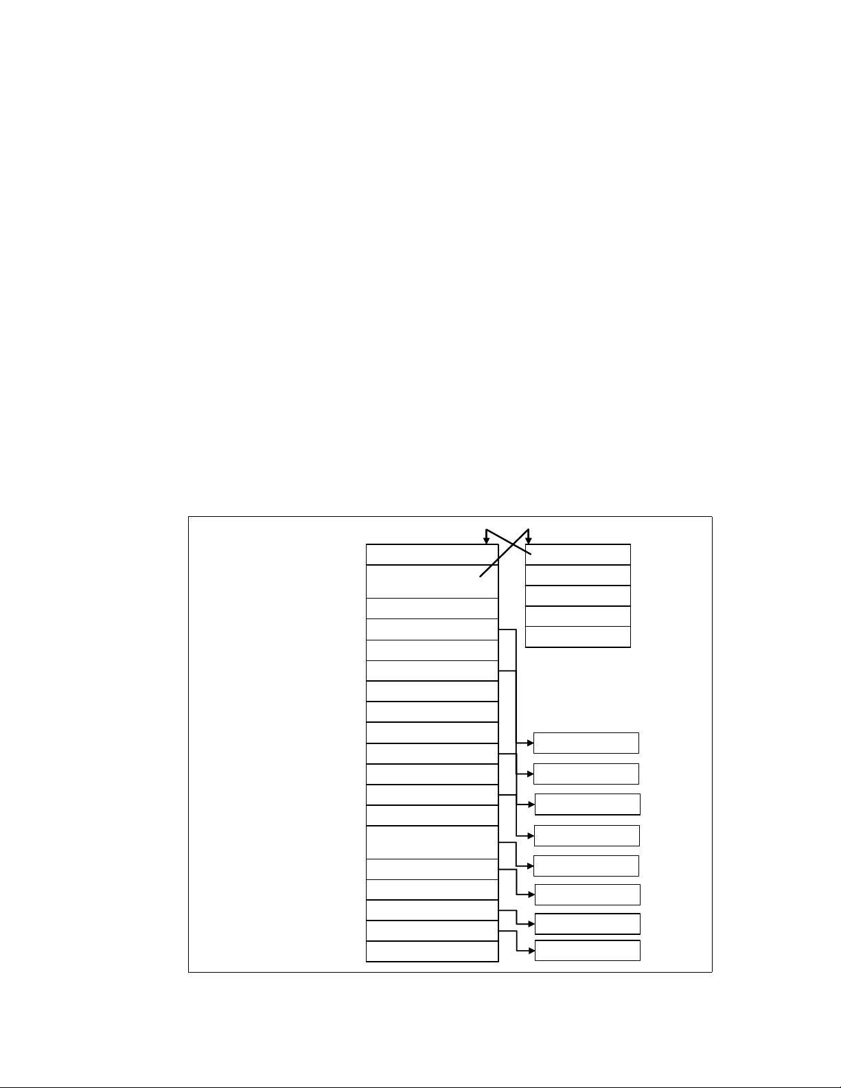
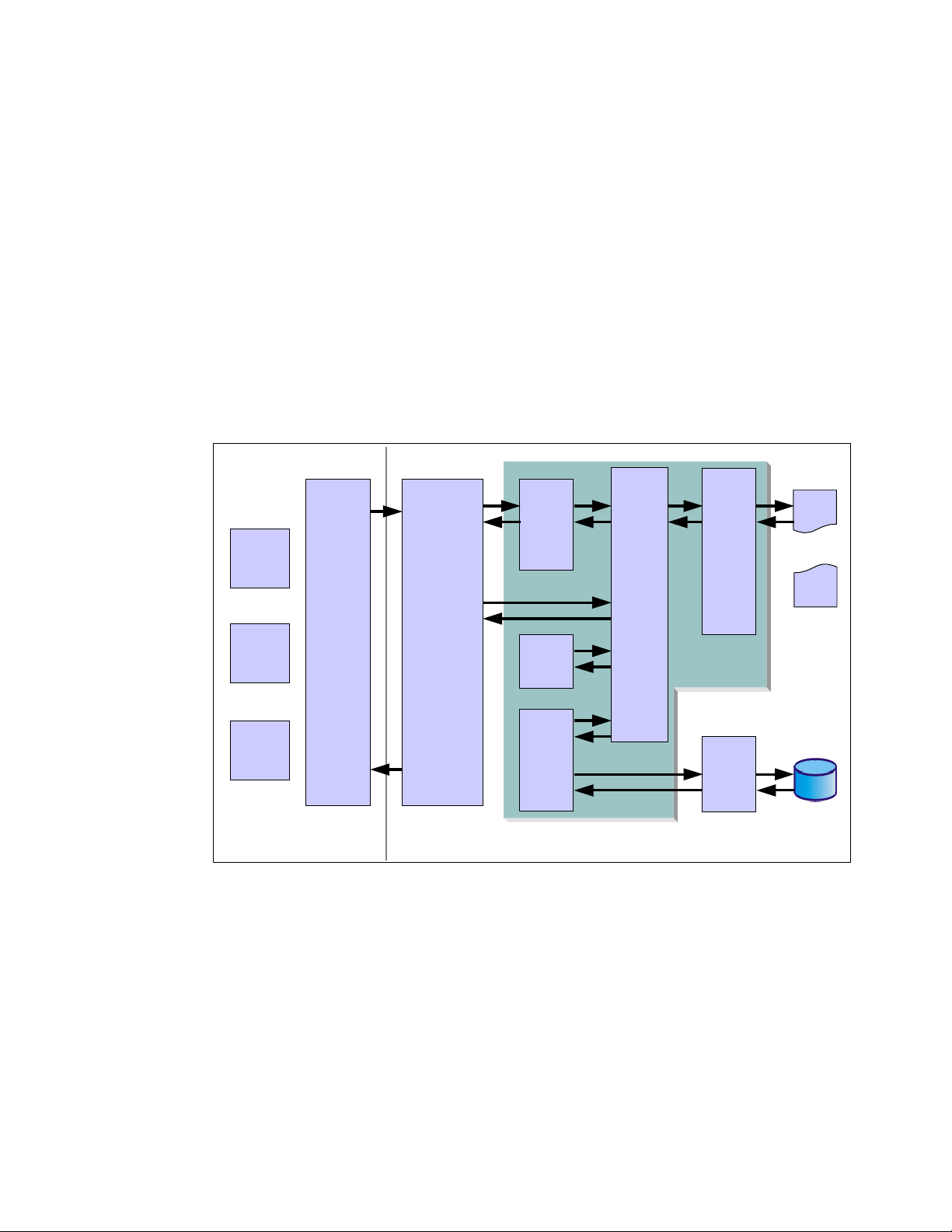
All processes running on Linux operating system are managed by the task_struct structure, which is also called necessary for a single process to run such as process identification, attributes of the process, resources which construct the process. If you know the structure of the process, you can understand what is important for process execution and performance. Figure 1-2 shows the outline of structures related to process information.

process descriptor. A process descriptor contains all the information

task_struct structure

kernel stack

Root directory

thread_info structure

task

stateProcess state

thread_infoProcess information and

run_list, arrayFor process scheduling

mmProcess address space

pidProcess ID

group_infoGroup management

userUser management

fsWorking directory

fliesFile descripter

signalSignal information

sighandSignal handler

task

exec_domain

flags

status

Kernel stack

the other structures

runqueue

mm_struct

group_info

user_struct

fs_struct

files_struct

signal_struct

sighand_struct

Figure 1-2 task_struct structure

Chapter 1. Understanding the Linux operating system 3

4285ch01.fm Draft Document for Review May 4, 2007 11:35 am

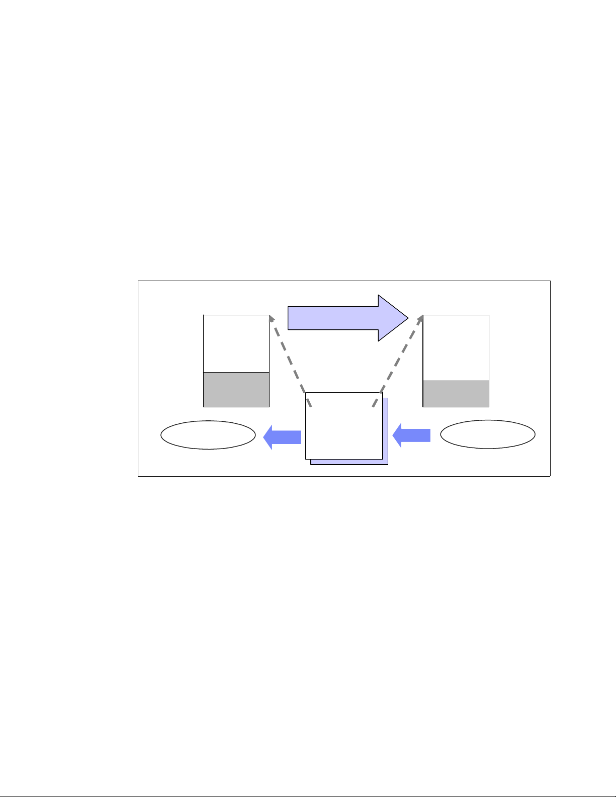
1.1.2 Lifecycle of a process

Every process has its own lifecycle such as creation, execution, termination and removal. These phases will be repeated literally millions of times as long as the system is up and running. Therefore, the process lifecycle is a very important topic from the performance perspective.

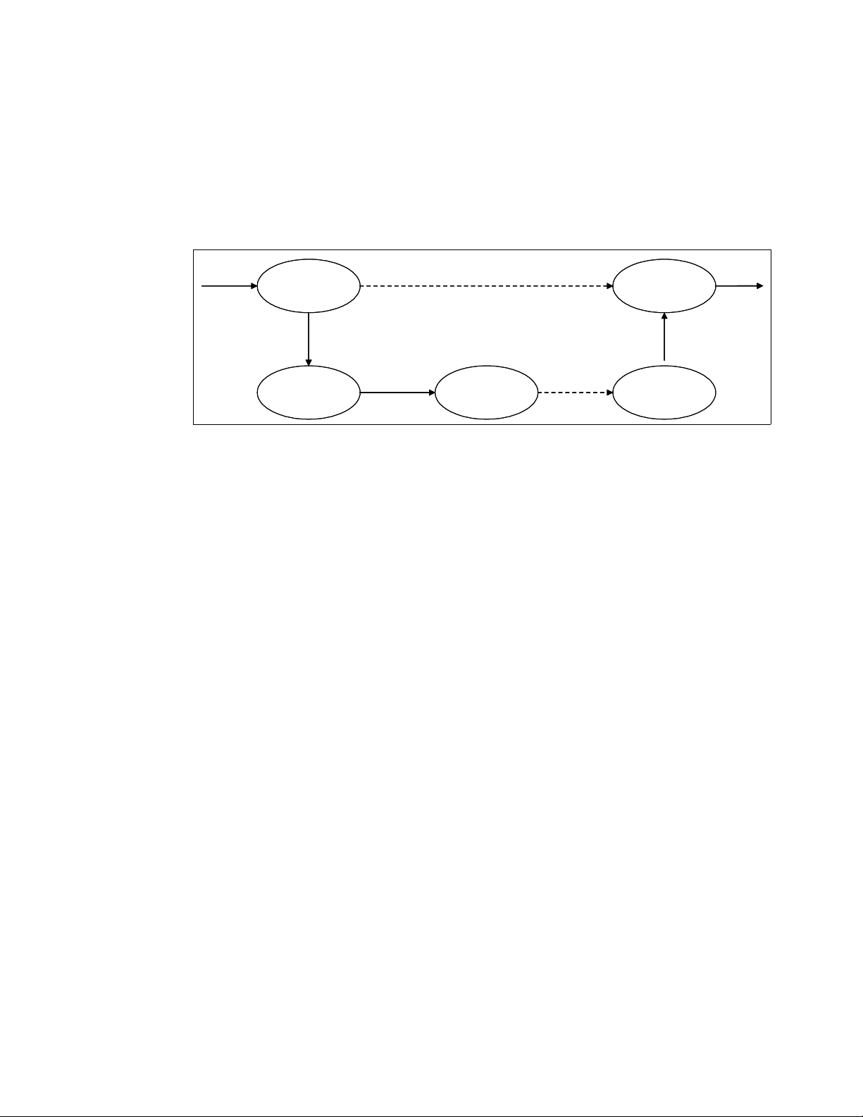
Figure 1-3 shows typical lifecycle of processes.

wait()

parent

process

fork()

parent

process

child

process

Figure 1-3 Lifecycle of typical processes

exec() exit()

child

process

zombie

process

When a process creates new process, the creating process (parent process) issues a fork() system call. When a fork() system call is issued, it gets a process descriptor for the newly created process (child process) and sets a new process id. It then copies the values of the parent process’s process descriptor to the child’s. At this time the entire address space of the parent process is not copied; both processes share the same address space.

The exec() system call copies the new program to the address space of the child process. Because both processes share the same address space, writing new program data causes a page fault exception. At this point, the kernel assigns the new physical page to the child process.

This deferred operation is called the

Copy On Write. The child process usually executes their

own program rather than the same execution as its parent does. This operation is a reasonable choice to avoid unnecessary overhead because copying an entire address space is a very slow and inefficient operation which uses much processor time and resources.

When program execution has completed, the child process terminates with an exit() system call. The exit() system call releases most of the data structure of the process, and notifies the parent process of the termination sending a certain signal. At this time, the process is called a

zombie process (refer to “Zombie processes” on page 8).

The child process will not be completely removed until the parent process knows of the termination of its child process by the wait() system call. As soon as the parent process is notified of the child process termination, it removes all the data structure of the child process and release the process descriptor.

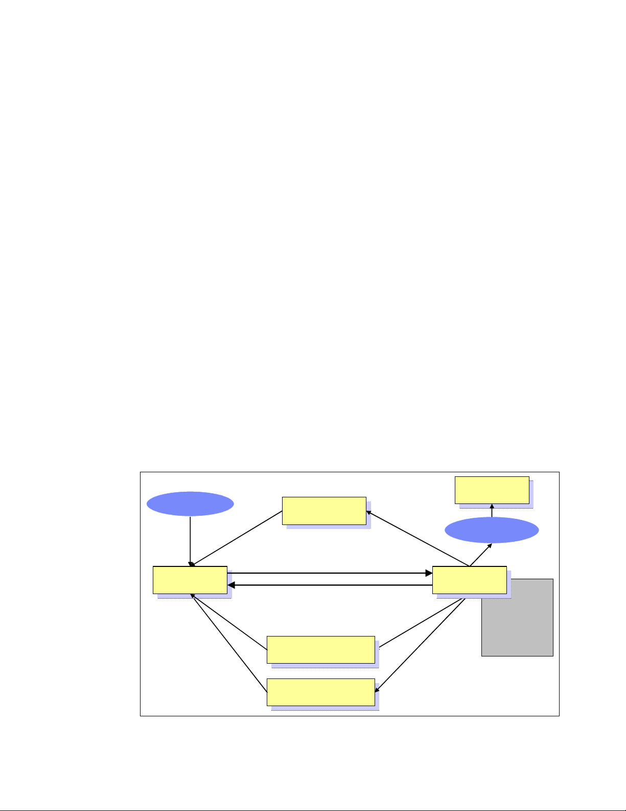
1.1.3 Thread

A thread is an execution unit which is generated in a single process and runs in parallel with other threads in the same process. They can share the same resources such as memory, address space, open files and so on. They can access the same set of application data. A thread is also called should take care not to change their shared resources at the same time. The implementation of mutual exclusion, locking and serialization etc. are the user application’s responsibility.

4 Linux Performance and Tuning Guidelines

Light Weight Process (LWP). Because they share resources, each thread

Draft Document for Review May 4, 2007 11:35 am 4285ch01.fm

resource

source

Threa

source

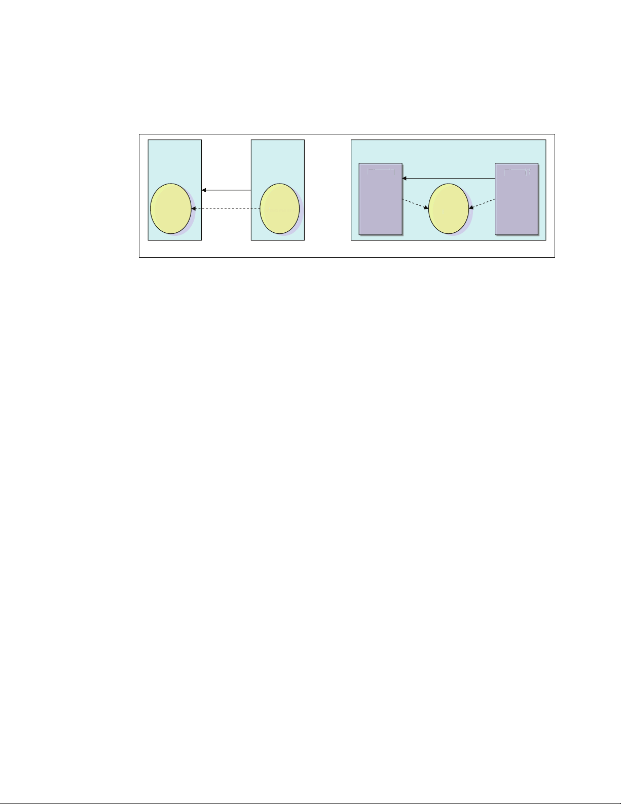
From the performance perspective, thread creation is less expensive than process creation because a thread does not need to copy resources on creation. On the other hand, processes and threads have similar characteristics in term of scheduling algorithm. The kernel deals with both of them in the similar manner.

Process Process

resource

copy

resource

Thread

Process

resource

share share

Thread

Process creation Thread creation

Figure 1-4 process and thread

In current Linux implementations, a thread is supported with the POSIX (Portable Operating System Interface for UNIX) compliant library (

pthread). There are several thread

implementations available in the Linux operating system. The following are the widely used.

򐂰 LinuxThreads

LinuxThreads have been the default thread implementation since Linux kernel 2.0 was available. The LinuxThread has some noncompliant implementations with the POSIX standard. NPTL is taking the place of LinuxThreads. The LinuxThreads will not be supported in future release of Enterprise Linux distributions.

򐂰 Native POSIX Thread Library (NPTL)

The NPTL was originally developed by Red Hat. NPTL is more compliant with POSIX standards. Taking advantage of enhancements in kernel 2.6 such as the new clone() system call, signal handling implementation etc., it has better performance and scalability than LinuxThreads.

There is some incompatibility with LinuxThreads. An application which has a dependence on LinuxThread may not work with the NPTL implementation.

򐂰 Next Generation POSIX Thread (NGPT)

NGPT is an IBM developed version of POSIX thread library. It is currently under maintenance operation and no further development is planned.

Using the LD_ASSUME_KERNEL environment variable, you can choose which threads library the application should use.

1.1.4 Process priority and nice level

Process priority is a number that determines the order in which the process is handled by the

CPU and is determined by dynamic priority and static priority. A process which has higher process priority has higher chances of getting permission to run on processor.

The kernel dynamically adjusts dynamic priority up and down as needed using a heuristic algorithm based on process behaviors and characteristics. A user process can change the static priority indirectly through the use of the higher static priority will have longer time slice (how long the process can run on processor).

nice level of the process. A process which has

Chapter 1. Understanding the Linux operating system 5

4285ch01.fm Draft Document for Review May 4, 2007 11:35 am

Linux supports nice levels from 19 (lowest priority) to -20 (highest priority). The default value is 0. To change the nice level of a program to a negative number (which makes it higher priority), it is necessary to log on or su to root.

1.1.5 Context switching

During process execution, information of the running process is stored in registers on processor and its cache. The set of data that is loaded to the register for the executing process is called the stored and the context of the next running process is restored to the register. The process descriptor and the area called kernel mode stack are used to store the context. This switching process is called because the processor has to flush its register and cache every time to make room for the new process. It may cause performance problems.

Figure 1-5 illustrates how the context switching works.

context. To switch processes, the context of the running process is

context switching. Having too much context switching is undesirable

task_struct

(Process A)

Figure 1-5 Context switching

1.1.6 Interrupt handling

Interrupt handling is one of the highest priority tasks. Interrupts are usually generated by I/O devices such as a network interface card, keyboard, disk controller, serial adapter, and so on. The interrupt handler notifies the Linux kernel of an event (such as keyboard input, ethernet frame arrival, and so on). It tells the kernel to interrupt process execution and perform interrupt handling as quickly as possible because some device requires quick responsiveness. This is critical for system stability. When an interrupt signal arrives to the kernel, the kernel must switch a currently execution process to new one to handle the interrupt. This means interrupts cause context switching, and therefore a significant amount of interrupts may cause performance degradation.

Address space of process A

stack

Suspend

Context switch

CPU

stack pointer

other registers

EIP register

etc.

Address space of process B

stack

task_struct

(Process B)

Resume

In Linux implementations, there are two types of interrupt. A devices which require responsiveness (disk I/O interrupt, network adapter interrupt, keyboard interrupt, mouse interrupt). A deferred (TCP/IP operation, SCSI protocol operation etc.). You can see information related to hard interrupts at /proc/interrupts.

6 Linux Performance and Tuning Guidelines

hard interrupt is generated for

soft interrupt is used for tasks which processing can be

Draft Document for Review May 4, 2007 11:35 am 4285ch01.fm

In a multi-processor environment, interrupts are handled by each processor. Binding interrupts to a single physical processor may improve system performance. For further details, refer to 4.4.2, “CPU affinity for interrupt handling”.

1.1.7 Process state

Every process has its own state to show what is currently happening in the process. Process state changes during process execution. Some of the possible states are as follows:

򐂰 TASK_RUNNING

In this state, a process is running on a CPU or waiting to run in the queue (run queue).

򐂰 TASK_STOPPED

A process suspended by certain signals (ex. SIGINT, SIGSTOP) is in this state. The process is waiting to be resumed by a signal such as SIGCONT.

򐂰 TASK_INTERRUPTIBLE

In this state, the process is suspended and waits for a certain condition to be satisfied. If a process is in TASK_INTERRUPTIBLE state and it receives a signal to stop, the process state is changed and operation will be interrupted. A typical example of a TASK_INTERRUPTIBLE process is a process waiting for keyboard interrupt.

򐂰 TASK_UNINTERRUPTIBLE

Similar to TASK_INTERRUPTIBLE. While a process in TASK_INTERRUPTIBLE state can be interrupted, sending a signal does nothing to the process in TASK_UNINTERRUPTIBLE state. A typical example of TASK_UNINTERRUPTIBLE process is a process waiting for disk I/O operation.

򐂰 TASK_ZOMBIE

After a process exits with exit() system call, its parent should know of the termination. In TASK_ZOMBIE state, a process is waiting for its parent to be notified to release all the data structure.

TASK_ZOMBIE

fork()

TASK_RUNNING

(READY) TASK_RUNNING

(READY)

TASK_STOPPED

Scheduling

Preemption

TASK_ZOMBIE

exit()

TASK_RUNNING

Processor

TASK_UNINTERRUPTIBLE

Figure 1-6 Process state

TASK_INTERRUPTIBLE

Chapter 1. Understanding the Linux operating system 7

4285ch01.fm Draft Document for Review May 4, 2007 11:35 am

Zombie processes

When a process has already terminated, having received a signal to do so, it normally takes some time to finish all tasks (such as closing open files) before ending itself. In that normally very short time frame, the process is a

After the process has completed all of these shutdown tasks, it reports to the parent process that it is about to terminate. Sometimes, a zombie process is unable to terminate itself, in which case it shows a status of Z (zombie).

It is not possible to kill such a process with the kill command, because it is already considered “dead.” If you cannot get rid of a zombie, you can kill the parent process and then the zombie disappears as well. However, if the parent process is the init process, you should not kill it. The init process is a very important process and therefore a reboot may be needed to get rid of the zombie process.

zombie.

1.1.8 Process memory segments

A process uses its own memory area to perform work. The work varies depending on the situation and process usage. A process can have different workload characteristics and different data size requirements. The process has to handle any of varying data sizes. To satisfy this requirement, the Linux kernel uses a dynamic memory allocation mechanism for each process. The process memory allocation structure is shown in Figure 1-7.

Text segment

Data segment

Heap segment

Stack segment

Figure 1-7 Process address space

Process address space

0x0000

Text

Executable instruction (Read-only

Data

Initialized data

BSS

Zero-ininitialized data

Heap

Dynamic memory allocation

by malloc()

Stack

Local variables

Function parameters,

Return address etc.

The process memory area consist of these segments

򐂰 Text segment

The area where executable code is stored.

8 Linux Performance and Tuning Guidelines

Draft Document for Review May 4, 2007 11:35 am 4285ch01.fm

򐂰 Data segment

The data segment consist of these three area.

– Data: The area where initialized data such as static variables are stored. – BSS: The area where zero-initialized data is stored. The data is initialized to zero. – Heap: The area where malloc() allocates dynamic memory based on the demand.

The heap grows toward higher addresses.

򐂰 Stack segment

The area where local variables, function parameters, and the return address of a function is stored. The stack grows toward lower addresses.

The memory allocation of a user process address space can be displayed with the pmap command. You can display the total size of the segment with the ps command. Refer to

2.3.10, “pmap” on page 52 and 2.3.4, “ps and pstree” on page 44.

1.1.9 Linux CPU scheduler

The basic functionality of any computer is, quite simply, to compute. To be able to compute, there must be a means to manage the computing resources, or processors, and the computing tasks, also known as threads or processes. Thanks to the great work of Ingo Molnar, Linux features a kernel using a O(1) algorithm as opposed to the O(n) algorithm used to describe the former CPU scheduler. The term O(1) refers to a static algorithm, meaning that the time taken to choose a process for placing into execution is constant, regardless of the number of processes.

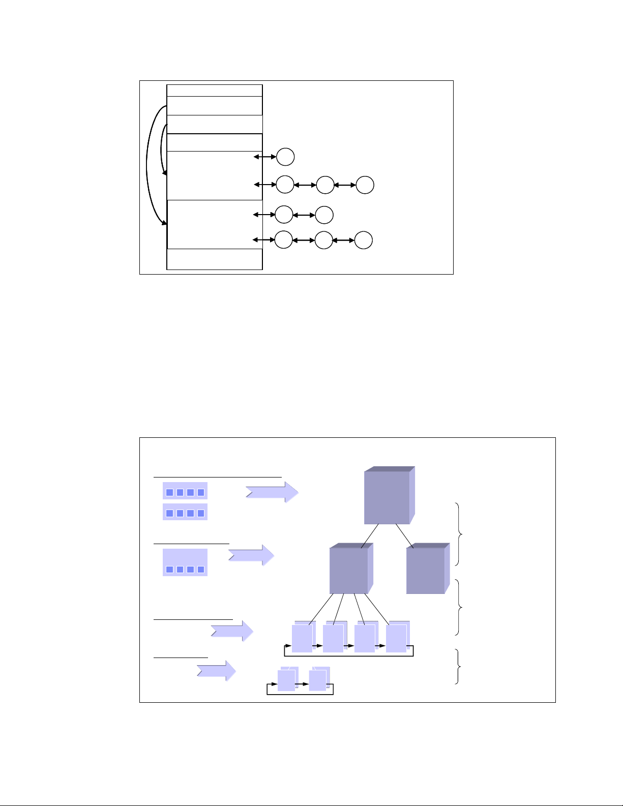
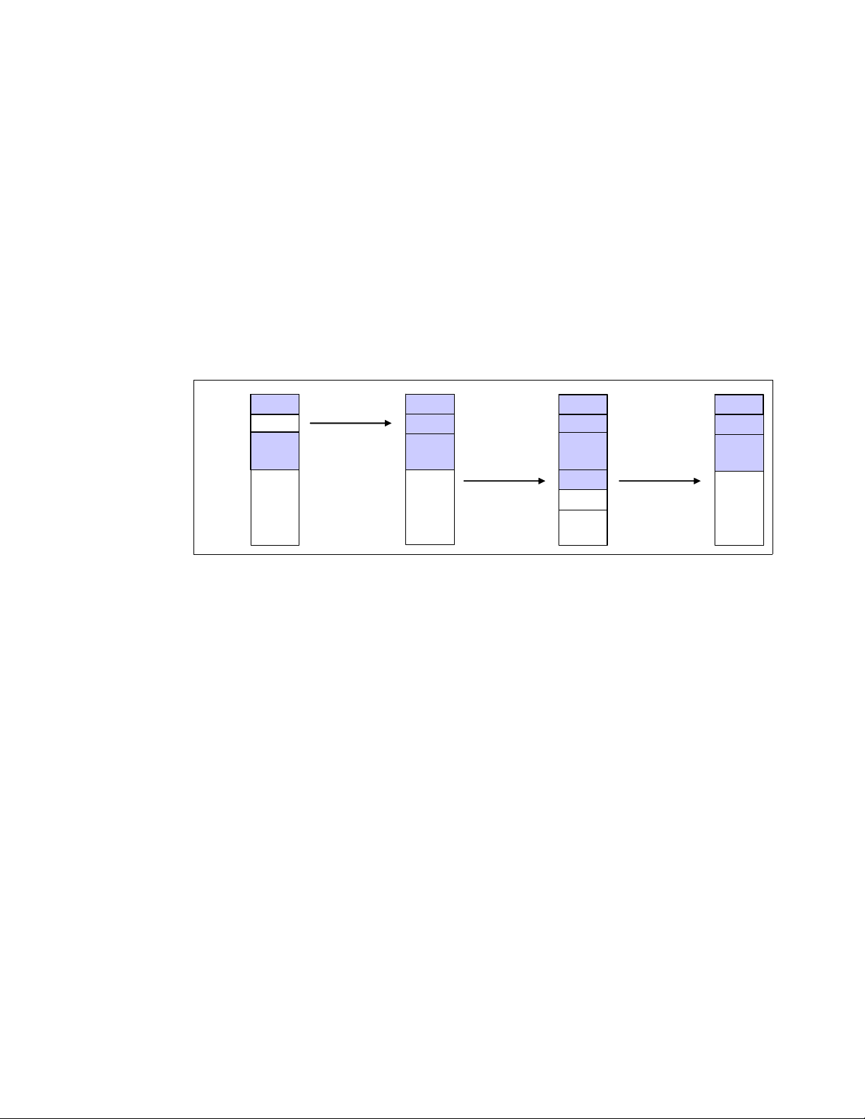
The new scheduler scales very well, regardless of process count or processor count, and imposes a low overhead on the system. The algorithm uses two process priority arrays:

򐂰 active 򐂰 expired

As processes are allocated a timeslice by the scheduler, based on their priority and prior blocking rate, they are placed in a list of processes for their priority in the active array. When they expire their timeslice, they are allocated a new timeslice and placed on the expired array. When all processes in the active array have expired their timeslice, the two arrays are switched, restarting the algorithm. For general interactive processes (as opposed to real-time processes) this results in high-priority processes, which typically have long timeslices, getting more compute time than low-priority processes, but not to the point where they can starve the low-priority processes completely. The advantage of such an algorithm is the vastly improved scalability of the Linux kernel for enterprise workloads that often include vast amounts of threads or processes and also a significant number of processors. The new O(1) CPU scheduler was designed for kernel 2.6 but backported to the 2.4 kernel family. Figure 1-8 illustrates how the Linux CPU scheduler works.

Chapter 1. Understanding the Linux operating system 9

4285ch01.fm Draft Document for Review May 4, 2007 11:35 am

active

expired

priority0

priority 139

priority0

priority 139

array[0]

array[1]

P P

Figure 1-8 Linux kernel 2.6 O(1) scheduler

Another significant advantage of the new scheduler is the support for Non-Uniform Memory Architecture (NUMA) and symmetric multithreading processors, such as Intel® Hyper-Threading technology.

The improved NUMA support ensures that load balancing will not occur across NUMA nodes unless a node gets overburdened. This mechanism ensures that traffic over the comparatively slow scalability links in a NUMA system are minimized. Although load balancing across processors in a scheduler domain group will be load balanced with every scheduler tick, workload across scheduler domains will only occur if that node is overloaded and asks for load balancing.

Parent Scheduler Domain

 Two node xSeries 445 (8 CPU)

 One CEC (4 CPU)

 One Xeon MP (HT)

 One HT CPU

Logical CPU

Scheduler Domain Group

1 2 …

Child Scheduler Domain

1 2 3 …

1 2 …

1 2 3 …

Load balancing only if a child is overburdened

1 2 3 …

Load balancing via scheduler_tick() and time slice

1 2 …

Load balancing via scheduler_tick()

Figure 1-9 Architecture of the O(1) CPU scheduler on an 8-way NUMA based system with Hyper-Threading enabled

10 Linux Performance and Tuning Guidelines

Draft Document for Review May 4, 2007 11:35 am 4285ch01.fm

1.2 Linux memory architecture

To execute a process, the Linux kernel allocates a portion of the memory area to the requesting process. The process uses the memory area as workspace and performs the required work. It is similar to you having your own desk allocated and then using the desktop to scatter papers, documents and memos to perform your work. The difference is that the kernel has to allocate space in more dynamic manner. The number of running processes sometimes comes to tens of thousands and amount of memory is usually limited. Therefore, Linux kernel must handle the memory efficiently. In this section, we describe the Linux memory architecture, address layout, and how the Linux manages memory space efficiently.

1.2.1 Physical and virtual memory

Today we are faced with the choice of 32-bit systems and 64-bit systems. One of the most important differences for enterprise-class clients is the possibility of virtual memory addressing above 4 GB. From a performance point of view, it is therefore interesting to understand how the Linux kernel maps physical memory into virtual memory on both 32-bit and 64-bit systems.

As you can see in Figure 1-10 on page 12, there are obvious differences in the way the Linux kernel has to address memory in 32-bit and 64-bit systems. Exploring the physical-to-virtual mapping in detail is beyond the scope of this paper, so we highlight some specifics in the Linux memory architecture.

On 32-bit architectures such as the IA-32, the Linux kernel can directly address only the first gigabyte of physical memory (896 MB when considering the reserved range). Memory above the so-called ZONE_NORMAL must be mapped into the lower 1 GB. This mapping is completely transparent to applications, but allocating a memory page in ZONE_HIGHMEM causes a small performance degradation.

On the other hand, with 64-bit architectures such as x86-64 (also x64), ZONE_NORMAL extends all the way to 64GB or to 128 GB in the case of IA-64 systems. As you can see, the overhead of mapping memory pages from ZONE_HIGHMEM into ZONE_NORMAL can be eliminated by using a 64-bit architecture.

Chapter 1. Understanding the Linux operating system 11

4285ch01.fm Draft Document for Review May 4, 2007 11:35 am

32-bit Architecture 64-bit Architecture

64GB

1GB

896MB

16MB

ZONE_HIGHMEM

~~ ~~

128MB

“Reserved”

ZONE_NORMAL

ZONE_DMA

Pages in ZONE_HIGHMEM must be mapped into ZONE_NORMAL

Reserved for Kernel data structures

64GB

1GB

ZONE_NORMAL

ZONE_DMA

Figure 1-10 Linux kernel memory layout for 32-bit and 64-bit systems

Virtual memory addressing layout

Figure 1-11 shows the Linux virtual addressing layout for 32-bit and 64-bit architecture.

On 32-bit architectures, the maximum address space that single process can access is 4GB. This is a restriction derived from 32-bit virtual addressing. In a standard implementation, the virtual address space is divided into a 3GB user space and a 1GB kernel space. There is some variants like 4G/4G addressing layout implementing.

On the other hand, on 64-bit architecture such as x86_64 and ia64, no such restriction exits. Each single process can enjoy the vast and huge address space.

32-bit Architecture

3G/1G kernel

0GB

User space

3GB

Kernel space

4GB

64-bit Architecture

x86_64

0GB

User space

Figure 1-11 Virtual memory addressing layout for 32bit and 64-bit architecture

512GB or more

Kernel space

12 Linux Performance and Tuning Guidelines

Draft Document for Review May 4, 2007 11:35 am 4285ch01.fm

1.2.2 Virtual memory manager

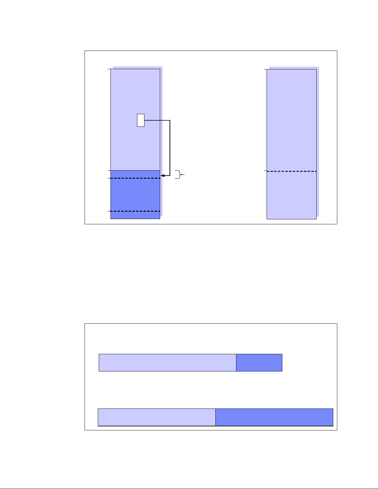
The physical memory architecture of an operating system usually is hidden to the application and the user because operating systems map any memory into virtual memory. If we want to understand the tuning possibilities within the Linux operating system, we have to understand how Linux handles virtual memory. As explained in 1.2.1, “Physical and virtual memory” on page 11, applications do not allocate physical memory, but request a memory map of a certain size at the Linux kernel and in exchange receive a map in virtual memory. As you can see in Figure 1-12 on page 13, virtual memory does not necessarily have to be mapped into physical memory. If your application allocates a large amount of memory, some of it might be mapped to the swap file on the disk subsystem.

Another enlightening fact that can be taken from Figure 1-12 on page 13 is that applications usually do not write directly to the disk subsystem, but into cache or buffers. The kernel threads then flushes out data in cache/buffers to the disk whenever it has time to do so (or, of course, if a file size exceeds the buffer cache). Refer to “Flushing dirty buffer” on page 22

pdflush

Physical

Kernel

Standard

httpd

mozilla

User Space

Processes

Figure 1-12 The Linux virtual memory manager

C Library

(glibc)

Subsystems

Slab Allocator

kswapd

bdflush

VM Subsystem

MMU

zoned buddy

allocator

Disk Driver

Memory

Disk

Closely connected to the way the Linux kernel handles writes to the physical disk subsystem is the way the Linux kernel manages disk cache. While other operating systems allocate only a certain portion of memory as disk cache, Linux handles the memory resource far more efficiently. The default configuration of the virtual memory manager allocates all available free memory space as disk cache. Hence it is not unusual to see productive Linux systems that boast gigabytes of memory but only have 20 MB of that memory free.

In the same context, Linux also handles swap space very efficiently. The fact that swap space is being used does not mean a memory bottleneck but rather proves how efficiently Linux handles system resources. See “Page frame reclaiming” on page 14 for more detail.

Chapter 1. Understanding the Linux operating system 13

4285ch01.fm Draft Document for Review May 4, 2007 11:35 am

Page frame allocation

A page is a group of contiguous linear addresses in physical memory (page frame) or virtual memory. The Linux kernel handles memory with this page unit. A page is usually 4K bytes in size. When a process requests a certain amount of pages, if there are available pages, the Linux kernel can allocate them to the process immediately. Otherwise pages have to be taken from some other process or page cache. The kernel knows how many memory pages are available and where they are located.

Buddy system

The Linux kernel maintains its free pages by using the mechanism called buddy system. The buddy system maintains free pages and tries to allocate pages for page allocation requests. It tries to keep the memory area contiguous. If small pages are scattered without consideration, it may cause memory fragmentation and it’s more difficult to allocate large portion of pages into a contiguous area. It may lead to inefficient memory use and performance decline. Figure 1-13 illustrates how the buddy system allocates pages.

2 pages

Used

chunk

Used

8 pages chunk

Figure 1-13 Buddy System

Request

for 2pages

8 pages chunk

Used

Request

for 2 pages

2 pages chunk

4 pages chunk

Used

Release

2 pages

8 pages chunk

Used

When the attempt of pages allocation failed, the page reclaiming will be activated. Refer to “Page frame reclaiming” on page 14.

You can find information on the buddy system through /proc/buddyinfo. For detail, please refer to “Memory used in a zone” on page 47.

Page frame reclaiming

If pages are not available when a process requests to map a certain amount of pages, the Linux kernel tries to get pages for the new request by releasing certain pages which are used before but not used anymore and still marked as active pages based on certain principals and allocating the memory to new process. This process is called thread and try_to_free_page() kernel function are responsible for page reclaiming.

page reclaiming. kswapd kernel

While kswapd is usually sleeping in task interruptible state, it is called by the buddy system when free pages in a zone fall short of a certain threshold. It then tries to find the candidate pages to be gotten out of active pages based on the Least Recently Used ( This is relatively simple. The pages least recently used should be released first. The active list and the inactive list are used to maintain the candidate pages. kswapd scans part of the active list and check how recently the pages were used then the pages not used recently is put into inactive list. You can take a look at how much memory is considered as active and inactive using vmstat -a command. For detail refer to 2.3.2, “vmstat”.

kswapd also follows another principal. The pages are used mainly for two purpose;

and process address space. The page cache is pages mapped to a file on disk. The

cache

pages belonging to a process address space is used for heap and stack (called anonymous memory because it‘s not mapped to any files, and has no name) (refer to 1.1.8, “Process

14 Linux Performance and Tuning Guidelines

LRU) principal.

page

Draft Document for Review May 4, 2007 11:35 am 4285ch01.fm

memory segments” on page 8). When kswapd reclaims pages, it would rather shrink the page cache than page out (or swap out) the pages owned by processes.

Note: The phrase “page out” and “swap out” is sometimes confusing. “page out” means take some pages (a part of entire address space) into swap space while “swap out” means taking entire address space into swap space. They are sometimes used interchangeably.

The good proportion of page cache reclaimed and process address space reclaimed may depend on the usage scenario and will have certain effects on performance. You can take some control of this behavior by using /proc/sys/vm/swappiness. Please refer to 4.5.1, “Setting kernel swap and pdflush behavior” on page 110 for tuning detail.

swap

As we stated before, when page reclaiming occurs, the candidate pages in the inactive list which belong to the process address space may be paged out. Having swap itself is not problematic situation. While swap is nothing more than a guarantee in case of over allocation of main memory in other operating systems, Linux utilizes swap space far more efficiently. As you can see in Figure 1-12, virtual memory is composed of both physical memory and the disk subsystem or the swap partition. If the virtual memory manager in Linux realizes that a memory page has been allocated but not used for a significant amount of time, it moves this memory page to swap space.

Often you will see daemons such as getty that will be launched when the system starts up but will hardly ever be used. It appears that it would be more efficient to free the expensive main memory of such a page and move the memory page to swap. This is exactly how Linux handles swap, so there is no need to be alarmed if you find the swap partition filled to 50%. The fact that swap space is being used does not mean a memory bottleneck but rather proves how efficiently Linux handles system resources.

1.3 Linux file systems

One of the great advantages of Linux as an open source operating system is that it offers users a variety of supported file systems. Modern Linux kernels can support nearly every file system ever used by a computer system, from basic FAT support to high performance file systems such as the journaling file system JFS. However, because Ext2, Ext3 and ReiserFS are native Linux file systems and are supported by most Linux distributions (ReiserFS is commercially supported only on Novell SUSE Linux), we will focus on their characteristics and give only an overview of the other frequently used Linux file systems.

For more information on file systems and the disk subsystem, see 4.6, “Tuning the disk subsystem” on page 113.

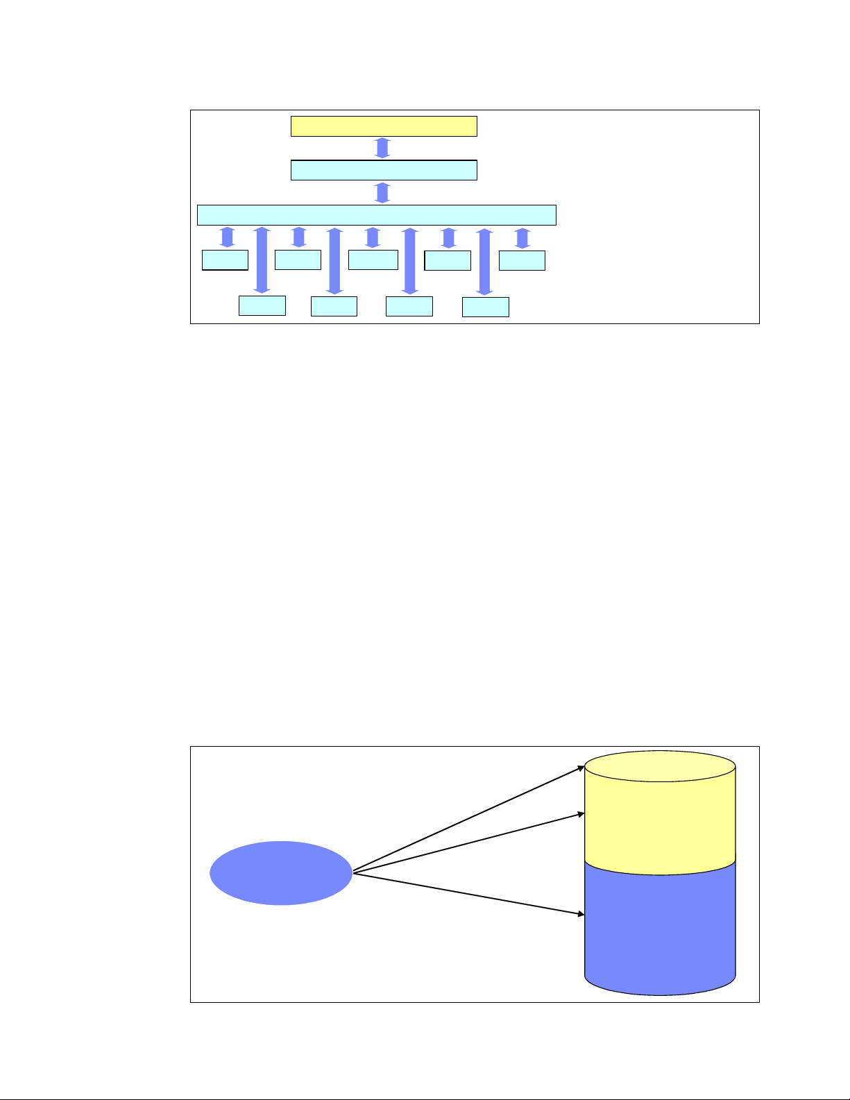
1.3.1 Virtual file system

Virtual Files System (VFS) is an abstraction interface layer that resides between the user process and various types of Linux file system implementations. VFS provides common object models (i.e. i-node, file object, page cache, directory entry etc.) and methods to access file system objects. It hides the differences of each file system implementation from user processes. Thanks to VFS, user processes do not need to know which file system to use, or which system call should be issued for each file system. Figure 1-14 illustrates the concept of VFS.

Chapter 1. Understanding the Linux operating system 15

4285ch01.fm Draft Document for Review May 4, 2007 11:35 am

ext2

Figure 1-14 VFS concept

1.3.2 Journaling

In a non-journaling file system, when a write is performed to a file system the Linux kernel makes changes to the file system metadata first and then writes actual user data next. This operations sometimes causes higher chances of losing data integrity. If the system suddenly crashes for some reason while the write operation to file system metadata is in process, the file system consistency may be broken. metadata and recover the consistency at the time of next reboot. But it takes way much time to be completed when the system has large volume. The system is not operational during this process.

NFS

ext3

AFS VFAT

User Process

System call

VFS

Reiserfs

open(), read(), write()

translation for each file system

XFS

JFS

proc

fsck will fix the inconsistency by checking all the

A Journaling file system solves this problem by writing data to be changed to the area called the journal area before writing the data to the actual file system. The journal area can be placed both in the file system itself or out of the file system. The data written to the journal area is called the journal log. It includes the changes to file system metadata and the actual file data if supported.

As journaling write journal logs before writing actual user data to the file system, it may cause performance overhead compared to no-journaling file system. How much performance overhead is sacrificed to maintain higher data consistency depends on how much information is written to disk before writing user data. We will discuss this topic in 1.3.4, “Ext3” on page 18.

write

Journal area

File system

Figure 1-15 Journaling concept

16 Linux Performance and Tuning Guidelines

Draft Document for Review May 4, 2007 11:35 am 4285ch01.fm

1.3.3 Ext2

The extended 2 file system is the predecessor of the extended 3 file system. A fast, simple file system, it features no journaling capabilities, unlike most other current file systems.

Figure 1-16 shows the Ext2 file system data structure. The file system starts with boot sector and followed by block groups. Splitting entire file system into several small block groups contributes performance gain because i-node table and data blocks which hold user data can resides closer on disk platter, then seek time can be reduced. A block group consist of:

Super block: Information on the file system is stored here. The exact copy of a

super block is placed in the top of every block group.

Block group descriptor: Information on the block group is stored.

Data block bitmaps: Used for free data block management.

i-node bitmaps: Used for free i-node management.

i-node tables: inode tables are stored here. Every file has a corresponding i-node

table which holds meta-data of the file such as file mode, uid, gid, atime, ctime, mtime, dtime and pointer to the data block.

Data blocks: Where actual user data is stored.

boot sector

BLOCK

Ext2

Figure 1-16 Ext2 file system data structure

GROUP 0

BLOCK

GROUP 1

BLOCK

GROUP 2

BLOCK

GROUP N

super block

block group

descriptors

data-block

bitmaps

inode

bitmaps

inode-table

Data-blocks

To find data blocks which consist of a file, the kernel searches the i-node of the file first. When a request to open /var/log/messages comes from a process, the kernel parses the file path and searches a directory entry of / (root directory) which has the information about files and directories under itself (root directory). Then the kernel can find the i-node of /var next and takes a look at the directory entry of /var, and it also has the information of files and directories under itself as well. The kernel gets down to the file in same manner until it finds

Chapter 1. Understanding the Linux operating system 17

4285ch01.fm Draft Document for Review May 4, 2007 11:35 am

i-node of the file. The Linux kernel uses file object cache such as directory entry cache, i-node cache to accelerate finding the corresponding i-node.

Now the Linux kernel knows i-node of the file then it tries to reach actual user data block. As we described, i-node has the pointer to the data block. By referring to it, the kernel can get to the data block. For large files, Ext2 implements direct/indirect reference to data block. Figure 1-17 illustrates how it works.

ext2 disk inode

i_size

direct

indirect

double indirect

trebly indirect

i_size

：

i_blocks

i_blocks[0]

i_blocks[1]

i_blocks[2]

i_blocks[3]

i_blocks[4]

i_blocks[5]

i_blocks[6]

i_blocks[7]

i_blocks[8]

i_blocks[9]

i_blocks[10]

i_blocks[11]

i_blocks[12]

i_blocks[13]

i_blocks[14]

Indirect

block

Data

block

Indirect

block

Indirect

block

Indirect

block

Data

block

Indirect

block

Indirect

block

Data block

Data

block

1.3.4 Ext3

Figure 1-17 Ext2 file system direct / indirect reference to data block

The file system structure and file access operations differ by file system. This makes different characteristics of each file system.

The current Enterprise Linux distributions support the extended 3 file system. This is an updated version of the widely used extended 2 file system. Though the fundamental structures are quite similar to Ext2 file system, the major difference is the support of journaling capability. Highlights of this file system include:

򐂰 Availability: Ext3 always writes data to the disks in a consistent way, so in case of an

unclean shutdown (unexpected power failure or system crash), the server does not have to spend time checking the consistency of the data, thereby reducing system recovery from hours to seconds.

򐂰 Data integrity: By specifying the journaling mode data=journal on the mount command, all

data, both file data and metadata, is journaled.

򐂰 Speed: By specifying the journaling mode data=writeback, you can decide on speed

versus integrity to meet the needs of your business requirements. This will be notable in environments where there are heavy synchronous writes.

򐂰 Flexibility: Upgrading from existing Ext2 file systems is simple and no reformatting is

necessary. By executing the tune2fs command and modifying the /etc/fstab file, you can easily update an Ext2 to an Ext3 file system. Also note that Ext3 file systems can be mounted as Ext2 with journaling disabled. Products from many third-party vendors have

18 Linux Performance and Tuning Guidelines

Draft Document for Review May 4, 2007 11:35 am 4285ch01.fm

the capability of manipulating Ext3 file systems. For example, PartitionMagic can handle the modification of Ext3 partitions.

Mode of journaling

Ext3 support three types of journaling mode.

򐂰 journal

This journaling option provides the highest form of data consistency by causing both file data and metadata to be journaled. It is also has the higher performance overhead.

򐂰 ordered

In this mode only metadata is written. However, file data is guaranteed to be written first. This is the default setting.

򐂰 writeback

This journaling option provides the fastest access to the data at the expense of data consistency. The data is guaranteed to be consistent as the metadata is still being logged. However, no special handling of actual file data is done and this may lead to old data appearing in files after a system crash.

1.3.5 ReiserFS

ReiserFS is a fast journaling file system with optimized disk-space utilization and quick crash recovery. ReiserFS has been developed to a great extent with the help of Novell. ReiserFS is commercially supported only on Novell SUSE Linux.

1.3.6 Journal File System

The Journal File System (JFS) is a full 64-bit file system that can support very large files and partitions. JFS was developed by IBM originally for AIX® and is now available under the general public license (GPL). JFS is an ideal file system for very large partitions and file sizes that are typically encountered in high performance computing (HPC) or database environments. If you would like to learn more about JFS, refer to:

http://jfs.sourceforge.net

Note: In Novell SUSE Linux Enterprise Server 10, JFS is no longer supported as a new file system.

1.3.7 XFS

The eXtended File System (XFS) is a high-performance journaling file system developed by Silicon Graphics Incorporated originally for its IRIX family of systems. It features characteristics similar to JFS from IBM by also supporting very large file and partition sizes. Therefore usage scenarios are very similar to JFS.

1.4 Disk I/O subsystem

Before a processor can decode and execute instructions, data should be retrieved all the way from sectors on a disk platter to processor cache and its registers and the results of the executions may be written back to the disk.

Chapter 1. Understanding the Linux operating system 19

4285ch01.fm Draft Document for Review May 4, 2007 11:35 am

We’ll take a look at Linux disk I/O subsystem to have better understanding of the components which have large effect on system performance.

1.4.1 I/O subsystem architecture

Figure 1-18 on page 20 shows basic concept of I/O subsystem architecture

User process

write()

VFS / file system layer

bio

block layer

device driver

file

page cache

I/O scheduler

I/O Request queue

Device driver

disk device

Disk

page

cache

page

cache

block buffer

pdflush

Figure 1-18 I/O subsystem architecture

For a quick understanding of overall I/O subsystem operations, we will take an example of writing data to a disk. The following sequence outlines the fundamental operations that occur when a disk-write operation is performed. Assuming that the file data is on sectors on disk platters and has already been read and is on the page cache.

1. A process requests to write a file through the write() system call

2. The kernel updates the

3. A

pdflush kernel thread takes care of flushing the page cache to disk

page cache mapped to the file

4. The file system layer puts each block buffer together to a layer” on page 23) and submits a write request to the block device layer

5. The block device layer gets requests from upper layers and performs an operation and puts the requests into the I/O request queue

20 Linux Performance and Tuning Guidelines

sector

bio struct (refer to 1.4.3, “Block

I/O elevator

Draft Document for Review May 4, 2007 11:35 am 4285ch01.fm

6. A device driver such as SCSI or other device specific drivers will take care of write operation

7. A disk device firmware do hardware operation like seek head, rotation, data transfer to the sector on the platter.

1.4.2 Cache

In the past 20 years, the performance improvement of processors has outperformed that of the other components in a computer system such as processor cache, bus, RAM, disk and so on. Slower access to memory and disk restricts overall system performance, so system performance is not be benefited by processor speed improvement. The cache mechanism resolves this problem by caching frequently used data in faster memory. It reduces the chances of having to access slower memory. Current computer system uses this technique in most all I/O components such as hard disk drive cache, disk controller cache, file system cache, cache handled by each application and so on.

Memory hierarchy

Figure 1-19 shows the concept of memory hierarchy. As the difference of access speed between the CPU register and disk is large, the CPU will spend much time waiting for data from slow disk devices, and therefore it significantly reduces the advantage of a fast CPU. Memory hierarchal structure reduces this mismatch by placing L1 cache, L2 cache, RAM and some other caches between the CPU and disk. It enables a process to get less chance to access slower memory and disk. The memory closer to processor has higher speed and less size.

This technique can also take advantage of locality of reference principal. The higher cache hit rate on faster memory is, the faster the access to data is.

very fast

CPU register

Figure 1-19 Memory hierarchy

Large speed mismatch

very slow

Disk

CPU

very fast

fast

cache

slow

RAM

very slow

Disk

Locality of reference

As we stated previously in “Memory hierarchy” above, achieving higher cache hit rate is the key for performance improvement. To achieve higher cache hit rate, the technique called “locality of reference” is used. This technique is based on the following principals:

򐂰 The data most recently used has a high probability of being used in near future (temporal

locality)

򐂰 The data resides close to the data which has been used has a high probability of being

used (spatial locality)

Figure 1-20 on page 22 illustrates this principal.

Chapter 1. Understanding the Linux operating system 21

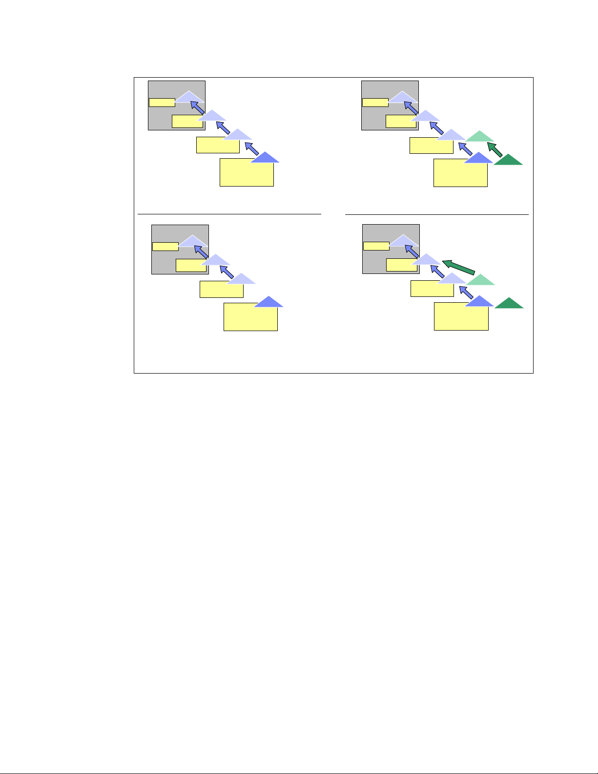
4285ch01.fm Draft Document for Review May 4, 2007 11:35 am

CPU

Data

Cache

Data

Memory

Disk

First access

CPU

Data

Cache

Data

Memory

Disk

Second access in a few seconds

Temporal locality

Data

CPU

Data

Cache

Data1

Disk

Data1

Data2

Data1

Data2

Data1

Disk

Memory

First access

CPU

Data

Cache

Memory

Second access to data2 in a few seconds

Spatial locality

Data2

Figure 1-20 Locality of reference

Linux implementation make use of this principal in many components such as page cache, file object cache (i-node cache, directory entry cache etc.), read ahead buffer and so on.

Flushing dirty buffer

When a process reads data from disk, the data is copied on to memory. The process and other processes can retrieve the same data from the copy of the data cached in memory. When a process tries to change the data, the process changes the data in memory first. At this time, the data on disk and the data in memory is not identical and the data in memory is referred to as a soon as possible, or the data in memory may be lost if a sudden crash occurs.

The synchronization process for a dirty buffer is called implementation, occurs on regular basis (kupdate) and when the proportion of dirty buffers in memory exceeds a certain threshold (bdflush). The threshold is configurable in the /proc/sys/vm/dirty_background_ratio file. For more information, refer to 4.5.1, “Setting kernel swap and pdflush behavior” on page 110.

dirty buffer. The dirty buffer should be synchronized to the data on disk as

flush. In the Linux kernel 2.6

pdflush kernel thread is responsible for flushing data to the disk. The flush

22 Linux Performance and Tuning Guidelines

Draft Document for Review May 4, 2007 11:35 am 4285ch01.fm

• Process read a data from disk

The data on memory and the data on disk are identical at this time.

• Process writes a new data

Only the data on memory has been changed, the data on disk and the data on memory is not the identical.

• Flushing writes the data on memory to the disk.

The data on disk is now identical to the data on memory.

Figure 1-21 Flushing dirty buffers

1.4.3 Block layer

The block layer handles all the activity related to block device operation (refer to Figure 1-18 on page 20). The key data structure in the block layer is the an interface between file system layer and block layer.

Process

read

write

Data

Cache

Data

Cache

Data

Cache

dirty buffer

flush

•pdflush

•sync()

Data

Disk

Data

Disk

Data

Disk

bio structure. The bio structure is

When a write is performed, file system layer tries to write to page cache which is made up of block buffers. It makes up a bio structure by putting the contiguous blocks together, then sends bio to the block layer. (refer to Figure 1-18 on page 20)

The block layer handles the bio request and links these requests into a queue called the I/O request queue. This linking operation is called

I/O elevator. In Linux kernel 2.6

implementations, four types of I/O elevator algorithms are available. These are described below.

Block sizes

The block size, the smallest amount of data that can be read or written to a drive, can have a direct impact on a server’s performance. As a guideline, if your server is handling many small files, then a smaller block size will be more efficient. If your server is dedicated to handling large files, a larger block size may improve performance. Block sizes cannot be changed on the fly on existing file systems, and only a reformat will modify the current block size.

I/O elevator

Apart from a vast amount of other features, the Linux kernel 2.6 employs a new I/O elevator model. While the Linux kernel 2.4 used a single, general-purpose I/O elevator, kernel 2.6 offers the choice of four elevators. Because the Linux operating system can be used for a wide range of tasks, both I/O devices and workload characteristics change significantly. A

Chapter 1. Understanding the Linux operating system 23

4285ch01.fm Draft Document for Review May 4, 2007 11:35 am

laptop computer quite likely has different I/O requirements from a 10,000-user database system. To accommodate this, four I/O elevators are available.

򐂰 Anticipatory

The anticipatory I/O elevator was created based on the assumption of a block device with only one physical seek head (for example a single SATA drive). The anticipatory elevator uses the deadline mechanism described in more detail below plus an anticipation heuristic. As the name suggests, the anticipatory I/O elevator “anticipates” I/O and attempts to write it in single, bigger streams to the disk instead of multiple very small random disk accesses. The anticipation heuristic may cause latency for write I/O. It is clearly tuned for high throughput on general purpose systems such as the average personal computer. Up to kernel release 2.6.18 the Anticipatory elevator is the standard I/O scheduler. However most Enterprise Linux distributions default to the CFQ elevator.

򐂰 Complete Fair Queuing (CFQ)

The CFQ elevator implements a QoS (Quality of Service) policy for processes by maintaining per-process I/O queues. The CFQ elevator is well suited for large multiuser systems with a vast amount of competing processes. It aggressively attempts to avoid starvation of processes and features low latency. Starting with kernel release 2.6.18 the improved CFQ elevator is the default I/O scheduler.

Depending on the system setup and the workload characterstic the CFQ scheduler can slowdown a single main application, for example a massive database with its fairness oriented algorithms. The default configuration handles the fairness based on process groups which compete against each other. For example a single database and also all writes via the page cache (all pdflush instances are in one pgroup) are considered as a single application by CFQ that may compete against many background processes. It can be useful to experiment with I/O scheduler subconfigurations and/or the deadline scheduler in such cases.

򐂰 Deadline

The deadline elevator is a cyclic elevator (round robin) with a deadline algorithm that provides a near real-time behavior of the I/O subsystem. The deadline elevator offers excellent request latency while maintaining good disk throughput. The implementation of the deadline algorithm ensures that starvation of a process cannot occur.

򐂰 NOOP

NOOP stands for No Operation, and the name explains most of its functionality. The NOOP elevator is simple and lean. It is a simple FIFO queue that performs no data ordering but simple merging of adjacent requests, so it adds very low processor overhead to disk I/O. The NOOP elevator assumes that a block device either features its own elevator algorithm such as TCQ for SCSI, or that the block device has no seek latency such as a flash card.

Note: With the Linux kernel release 2.6.18 the I/O elevators are now selectable on a per disk subsystem basis and have no longer to be set on a per system level.

1.4.4 I/O device driver

The Linux kernel takes control of devices using a device driver. The device driver is usually a separate kernel module and is provided for each device (or group of devices) to make the device available for the Linux operating system. Once the device driver is loaded, it runs as a part of the Linux kernel and takes full control of the device. Here we describe SCSI device drivers.

24 Linux Performance and Tuning Guidelines

Draft Document for Review May 4, 2007 11:35 am 4285ch01.fm

SCSI

The Small Computer System Interface (SCSI) is the most commonly used I/O device technology, especially in the enterprise server environment. In Linux kernel implementations, SCSI devices are controlled by device driver modules. They consist of the following types of modules.

򐂰 Upper level drivers: sd_mod, sr_mod(SCSI-CDROM), st(SCSI Tape), sq(SCSI generic

device) etc.

Provide functionalities to support several types of SCSI devices such as SCSI CD-ROM, SCSI tape etc.

򐂰 Middle level driver: scsi_mod

Implements SCSI protocol and common SCSI functionality

򐂰 Low level drivers

Provide lower level access to each devices. Low level driver is basically specific to a hardware device and provided for each device. For example, ips for IBM ServeRAID™ controller, qla2300 for Qlogic HBA, mptscsih for LSI Logic SCSI controller etc.

򐂰 Pseudo driver: ide-scsi

Used for IDE-SCSI emulation.

st sr_modsd_modsg

ips qla2300mptscsih

Figure 1-22 Structure of SCSI drivers

If there is specific functionality implemented for a device, it should be implemented in device firmware and the low level device driver. The supported functionality depend on which hardware you use and which version of device driver you use. The device itself should also support the desired functionality. Specific functions are usually tuned by a device driver parameter. You may try some performance tuning in /etc/modules.conf. Refer to the device and device driver documentation for possible tuning hints and tips.

1.4.5 RAID and Storage system

The selection and configuration of storage system and RAID types are also important factors in terms of system performance. However we leave the details of this topic out of scope of this Redpaper, though Linux supports software RAID. We include some of tuning considerations in 4.6.1, “Hardware considerations before installing Linux” on page 114.

Process

scsi_mod

Device

……

Upper level driver

Mid level driver

Low level driver

For additional, in-depth coverage of the available IBM storage solutions, see:

򐂰 Tuning IBM System x Servers for Performance, SG24-5287

򐂰 IBM System Storage Solutions Handbook, SG24-5250

򐂰 Introduction to Storage Area Networks, SG24-5470

Chapter 1. Understanding the Linux operating system 25

4285ch01.fm Draft Document for Review May 4, 2007 11:35 am

1.5 Network subsystem

The network subsystem is another important subsystem in the performance perspective. Networking operations interact with many components other than Linux itself such as switches, routers, gateways, PC clients etc. Though these components may be out of the control of Linux, they have much influence on the overall performance. Keep in mind that you have to work closely with people working on the network system.

Here we mainly focus on how Linux handles networking operations.

1.5.1 Networking implementation

The TCP/IP protocol has a layered structure similar to the OSI layer model. The Linux kernel networking implementation employs a similar approach. Figure 1-23 illustrates the layered Linux TCP/IP stack and quick overview of TCP/IP communication.

Process

BSD socket

Ethernet

Header

IP Header

TCP/UDP

Header

Data

sk_buff

INET socket

TCP/UDP

Datalink

Device

Device driver

NIC

Figure 1-23 Network layered structure and quick overview of networking operation

Linux uses a socket interface for TCP/IP networking operation as well as many UNIX systems do. The socket provides an interface for user applications. We will take a quick look at the sequence that outlines the fundamental operations that occur during network data transfer.

1. When an application sends data to its peer host, the application creates its data.

2. The application opens the socket and writes the data through the socket interface.

3. The

4. In each layer, appropriate operations such as parsing the headers, adding and modifying

socket buffer is used to deal with the transferred data. The socket buffer has reference

to the data and it goes down through the layers.

the headers, check sums, routing operation, fragmentation etc. are performed. When the socket buffer goes down through the layers, the data itself is not copied between the layers. Because copying actual data between different layer is not effective, the kernel avoids unnecessary overhead by just changing the reference in the socket buffer and passing it to the next layer.

Process

BSD socket

INET socket

TCP/UDP

Datalink

Device

Device driver

NIC

5. Finally the data goes out to the wire from network interface card.

6. The Ethernet frame arrives at the network interface of the peer host

26 Linux Performance and Tuning Guidelines

Draft Document for Review May 4, 2007 11:35 am 4285ch01.fm

7. The frame is moved into the network interface card buffer if the MAC address matches the MAC address of the interface card.

8. The network interface card eventually moves the packet into a socket buffer and issues a hard interrupt at the CPU.

9. The CPU then processes the packet and moves it up through the layers until it arrives at (for example) a TCP port of an application such as Apache.

Socket buffer

As we stated before, the kernel uses buffers to send and receive data. Figure 1-24 shows configurable buffers which can be used for networking. They can be tuned through files in

/proc/sys/net.

/proc/sys/net/core/rmem_max /proc/sys/net/core/rmem_default /proc/sys/net/core/wmem_max /proc/sys/net/core/wmem_default /proc/sys/net/ipv4/tcp_mem /proc/sys/net/ipv4/tcp_rmem /proc/sys/net/ipv4/tcp_wmem

Sometimes it may have an effect on the network performance. We’ll cover the details in 4.7.4, “Increasing network buffers” on page 127.

tcp_rmem

tcp_wmem

rmem_max

TCP/IP

receive

IPX

tcp_mem

socket

buffer

socket

r s

socket

wmem_max

send

buffer

tcp_mem

socket

send

buffer

receive

buffer

tcp_mem

socket

r s

Appletalk

Figure 1-24 socket buffer memory allocation

Chapter 1. Understanding the Linux operating system 27

4285ch01.fm Draft Document for Review May 4, 2007 11:35 am

Network API (NAPI)

The network subsystem has undergone some changes with the introduction of the new network API (NAPI). The standard implementation of the network stack in Linux focuses more on reliability and low latency than on low overhead and high throughput. While these characteristics are favorable when creating a firewall, most enterprise applications such as file and print or databases will perform more slowly than a similar installation under Windows®.

In the traditional approach of handling network packets, as depicted by the blue arrows in Figure 1-25, the network interface card eventually moves the packet into a network buffer of the operating systems kernel and issues a hard interrupt at the CPU, as we stated before.

This is only a simplified view of the process of handling network packets, but it illustrates one of the shortcomings of this very approach. As you have realized, every time an Ethernet frame with a matching MAC address arrives at the interface, there will be a hard interrupt. Whenever a CPU has to handle a hard interrupt, it has to stop processing whatever it was working on and handle the interrupt, causing a context switch and the associated flush of the processor cache. While one might think that this is not a problem if only a few packets arrive at the interface, Gigabit Ethernet and modern applications can create thousands of packets per second, causing a vast number of interrupts and context switches to occur.

ip_rcv() arp_rcv()

netif_receive_skb(skb)

process_backlog(struct net_device *backlog_dev, int *budget)

net/core/dev.c:net_rx_action(struct softirq_action *h)

/net/core/dev.c_raise_softirq_irqoff(NET_RX)SOFTIRQ)

/net/core/dev.c:_netif_rx_schedule(&queue->backlog_dev)

/net/core/dev.c:int netif_rx(struct sk_buff *skb)

NAPI way

Figure 1-25 The Linux network stack

28 Linux Performance and Tuning Guidelines

DEVICE

Draft Document for Review May 4, 2007 11:35 am 4285ch01.fm

Because of this, NAPI was introduced to counter the overhead associated with processing network traffic. For the first packet, NAPI works just like the traditional implementation as it issues an interrupt for the first packet. But after the first packet, the interface goes into a polling mode: As long as there are packets in the DMA ring buffer of the network interface, no new interrupts will be caused, effectively reducing context switching and the associated overhead. Should the last packet be processed and the ring buffer be emptied, then the interface card will again fall back into the interrupt mode we explored earlier. NAPI also has the advantage of improved multiprocessor scalability by creating soft interrupts that can be handled by multiple processors. While NAPI would be a vast improvement for most enterprise class multiprocessor systems, it requires NAPI-enabled drivers. There is significant room for tuning, as we will explore in the tuning section of this Redpaper.

Netfilter

Linux has an advanced firewall capability as a part of the kernel. This capability is provided by

Netfilter modules. You can manipulate and configure Netfilter using iptables utility.

Generally speaking, Netfilter provides the following functions.

򐂰 Packet filtering: If a packet match a certain rule, Netfilter accept or deny the packets or

take appropriate action based on defined rules

򐂰 Address translation: If a packet match a certain rule, Netfilter alter the packet itself to meet

the address translation requirements.

Matching filters can be defined with the following properties.

򐂰 Network interface

򐂰 IP address, IP address range, subnet

򐂰 Protocol

򐂰 ICMP Type

򐂰 Por t

򐂰 TCP flag

򐂰 State (refer to “Connection tracking” on page 30)

Figure 1-26 give an overview of how packets traverse the Netfilter chains which are the lists of defined rules applied at each point in sequence.

incoming packets

PREROUTINGPREROUTING

Connection Tracking Mangle NAT(DNAT)

ROUTING

incoming packets

INPUTINPUT

forwarded packets

FORWARDFORWARD

Filter

Connection Tracking Filter

OUTPUTOUTPUT

originated from local process

Connection Tracking NAT(SNAT,MASQUERADE)

POSTROUTINGPOSTROUTING

outgoing packets

Connection Tracking Mangle NAT(DNAT) Filter

Local process

Figure 1-26 Netfilter packet flow

Netfilter will take appropriate actions if packet matches the rule. The action is called a target. Some of possible targets are:

Chapter 1. Understanding the Linux operating system 29

4285ch01.fm Draft Document for Review May 4, 2007 11:35 am

ACCEPT: Accept the packet and let it through. DROP: Silently discard the packet. REJECT: Discard the packet with sending back the packet such as ICMP port

unreachable, TCP reset to originating host. LOG: Logging matching packet. MASQUERADE, SNAT, DNAT, REDIRECT:Address translation

Connection tracking

To achieve more sophisticated firewall capability, Netfilter employes the connection tracking mechanism which keeps track of the state of all network traffic. Using the TCP connection state (refer to “Connection establishment” on page 30) and other network properties (such as IP address, port, protocol, sequence number, ack number, ICMP type etc.), Netfilter classifies each packet to the following four states.

NEW: packet attempting to establish new connection ESTABLISHED: packet goes through established connection RELATED: packet which is related to previous packets INVALID: packet which is unknown state due to malformed or invalid packet

In addition, Netfilter can use a separate module to perform more detailed connection tracking by analyzing protocol specific properties and operations. For example, there are connection tracking modules for FTP, NetBIOS, TFTP, IRC and so on.

1.5.2 TCP/IP

TCP/IP has been default network protocol for many years. Linux TCP/IP implementation is fairly compliant with its standards. For better performance tuning, you should be familiar with basic TCP/IP networking.

For additional detail refer to the following documentation:

TCP/IP Tutorial and Technical Overview, SG24-3376.

Connection establishment

Before application data is transferred, the connection should be established between client and server. The connection establishment process is called TCP/IP 3-way hand shake. Figure 1-27 on page 31 outlines basic connection establishment and termination process.

1. A client sends a SYN packet (a packet with SYN flag set) to its peer server to request

connection.

2. The server receives the packet and sends back SYN+ACK packet

3. Then the client sends an ACK packet to its peer to complete connection establishment.

Once the connection is established, the application data can be transferred through the connection. When all data has been transferred, the connection closing process starts.

1. The client sends a FIN packet to the server to start the connection termination process.

2. The server sends the acknowledgement of the FIN back and then sends the FIN packet to

the client if it has no data to send to the client.

3. Then the client sends an ACK packet to the server to complete connection termination.

30 Linux Performance and Tuning Guidelines

Draft Document for Review May 4, 2007 11:35 am 4285ch01.fm

Client

send SYN

SYN_SENT

receive SYN+ACK

ESTABLISHED

receive FIN

FIN_WAIT1

receive ACK

FIN_WAIT2

receive FIN

TIME_WAIT

send ACK

TimeOut

CLOSED

SYN

SYN+ACK

ACK

TCP session established

FIN

ACK

FIN

ACK

Server

LISTEN

receive SYN

SYN_RECV

SYN＋ACK sent

receive ACK

ESTABLISHED

receivr FIN

CLOSE_WAIT

receive ACK

reveive FIN

LAST_ACK

receive ACK

CLOSED

Figure 1-27 TCP 3-way handshake

The state of a connection changes during the session. Figure 1-28 on page 32 show the TCP/IP connection state diagram.

Chapter 1. Understanding the Linux operating system 31

4285ch01.fm Draft Document for Review May 4, 2007 11:35 am

active OPEN

create TCB

snd SYN

SYN

SENT

RCVD

snd FIN

SYN

FIN

passive

OPEN

create TCB

rcv SYN

snd

SYN,ACK

rcv ACK of

SYN

snd FIN

CLOSED

LISTEN

rcv SYN

snd ACK

ESTAB

delete

TCB

SEND snd SYN

SYN,ACK

rcv FIN

snd

ACK

CLOSE delete TCB

rcv

snd ACK

WAIT-1

rcv ACK of FIN

FIN

rcv FIN

snd

ACK

rcv ACK of

rcv FIN

snd

ACK

WAIT-2

Figure 1-28 TCP connection state diagram

You can see the connection state of each TCP/IP session using netstat command. For more detail, see 2.3.11, “netstat” on page 53.

Traffic control

TCP/IP implementation has a mechanism that ensures efficient data transfer and guarantees packet delivery even in time of poor network transmission quality and congestion.

TCP/IP transfer window

The principle of transfer windows is an important aspect of the TCP/IP implementation in the Linux operating system in regard to performance. Very simplified, the TCP transfer window is the maximum amount of data a given host can send or receive before requiring an acknowledgement from the other side of the connection. The window size is offered from the receiving host to the sending host by the window size field in the TCP header. Using the transfer window, the host can send packets more effectively because the sending host doesn’t have to wait for acknowledgement for each sending packet. It enables the network to be utilized more. Delayed acknowledgement also improve efficiency. TCP windows start small and increase slowly with every successful acknowledgement from the other side of the connection. To optimize window size, see 4.7.4, “Increasing network buffers” on page 127

CLOSING

FIN

TIME WAIT

Timeout=2MSL

delete TCB

WAIT

LAST-ACK

CLOSED

snd FIN

rcv ACK of

FIN

32 Linux Performance and Tuning Guidelines

Draft Document for Review May 4, 2007 11:35 am 4285ch01.fm

Sender Receiver

Figure 1-29 Sliding window and delayed ack

Sender Receiver

Sliding window

Delayed Ack

As an option, high-speed networks may use a technique called window scaling to increase the maximum transfer window size even more. We will analyze the effects of these implementations in more detail in “Tuning TCP options” on page 132.

Retransmission

In the connection establishment and termination and data transfer, many timeouts and data retransmissions may be caused by various reasons (faulty network interface, slow router, network congestion, buggy network implementation, and so on). TCP/IP handles this situation by queuing packets and trying to send packets several times.

You can change some behavior of the kernel by configuring parameters. You may want to increase the number of attempts for TCP SYN connection establishment packet on the network with high rate of packet loss. You can also change some of timeout threshold through files under /proc/sys/net. For more information, see “Tuning TCP behavior” on page 131.

1.5.3 Offload

If the network adapter on your system supports hardware offload functionality, the kernel can offload part of its task to the adapter and it can reduce CPU utilization.

򐂰 Checksum offload

򐂰 TCP segmentation offload (TSO)

For more advanced network features, refer to redbook Tuning IBM System x Servers for Performance, SG24-5287. section 10.3. Advanced network features.

IP/TCP/UDP checksum is performed to make sure if the packet is correctly transferred by comparing the value of checksum field in protocol headers and the calculated values by the packet data.

When the data that is lager than supported maximum transmission unit (MTU) is sent to the network adapter, the data should be divided into MTU sized packets. The adapter takes care of that on behalf of the kernel.

Chapter 1. Understanding the Linux operating system 33

4285ch01.fm Draft Document for Review May 4, 2007 11:35 am

1.5.4 Bonding module

The Linux kernel provides network interface aggregation capability by using a bonding driver. This is a device independent bonding driver, while there are device specific drivers as well. The bonding driver supports the 802.3 link aggregation specification and some original load balancing and fault tolerant implementations as well. It achieves a higher level of availability and performance improvement. Please refer to the kernel documentation Documentation/networking/bonding.txt.

1.6 Understanding Linux performance metrics

Before we can look at the various tuning parameters and performance measurement utilities in the Linux operating system, it makes sense to discuss various available metrics and their meaning in regard to system performance. Because this is an open source operating system, a significant amount of performance measurement tools are available. The tool you ultimately choose will depend upon your personal liking and the amount of data and detail you require. Even though numerous tools are available, all performance measurement utilities measure the same metrics, so understanding the metrics enables you to use whatever utility you come across. Therefore, we cover only the most important metrics, understanding that many more detailed values are available that might be useful for detailed analysis beyond the scope of this paper.

1.6.1 Processor metrics

򐂰 CPU utilization

This is probably the most straightforward metric. It describes the overall utilization per processor. On IBM System x architectures, if the CPU utilization exceeds 80% for a sustained period of time, a processor bottleneck is likely.

򐂰 User time

Depicts the CPU percentage spent on user processes, including nice time. High values in user time are generally desirable because, in this case, the system performs actual work.

򐂰 System time

Depicts the CPU percentage spent on kernel operations including IRQ and softirq time. High and sustained system time values can point you to bottlenecks in the network and driver stack. A system should generally spend as little time as possible in kernel time.

򐂰 Waiting

Total amount of CPU time spent waiting for an I/O operation to occur. Like the value, a system should not spend too much time waiting for I/O operations; otherwise you should investigate the performance of the respective I/O subsystem.

򐂰 Idle time

Depicts the CPU percentage the system was idle waiting for tasks.

򐂰 Nice time

blocked

Depicts the CPU percentage spent on re-nicing processes that change the execution order and priority of processes.

򐂰 Load average

The load average is not a percentage, but the rolling average of the sum of the followings:

– the number of processes in queue waiting to be processed – the number of processes waiting for uninterruptable task to be completed

34 Linux Performance and Tuning Guidelines

Draft Document for Review May 4, 2007 11:35 am 4285ch01.fm

That is, the average of the sum of TASK_RUNNING and TASK_UNINTERRUPTIBLE process. If processes that request CPU time are blocked (which means that the CPU has no time to process them), the load average will increase. On the other hand, if each process gets immediate access to CPU time and there are no CPU cycles lost, the load will decrease.

򐂰 Runable processes

This value depicts the processes that are ready to be executed. This value should not exceed 10 times the amount of physical processors for a sustained period of time; otherwise a processor bottleneck is likely.

򐂰 Blocked

Processes that cannot execute as they are waiting for an I/O operation to finish. Blocked processes can point you toward an I/O bottleneck.

򐂰 Context switch

Amount of switches between threads that occur on the system. High numbers of context switches in connection with a large number of interrupts can signal driver or application issues. Context switches generally are not desirable because the CPU cache is flushed with each one, but some context switching is necessary. Refer to 1.1.5, “Context switching” on page 6.

򐂰 Interrupts

The interrupt value contains hard interrupts and soft interrupts; hard interrupts have more of an adverse effect on system performance. High interrupt values are an indication of a software bottleneck, either in the kernel or a driver. Remember that the interrupt value includes the interrupts caused by the CPU clock. Refer to 1.1.6, “Interrupt handling” on page 6

1.6.2 Memory metrics

򐂰 Free memor y

Compared to most other operating systems, the free memory value in Linux should not be a cause for concern. As explained in 1.2.2, “Virtual memory manager” on page 13, the Linux kernel allocates most unused memory as file system cache, so subtract the amount of buffers and cache from the used memory to determine (effectively) free memory.

򐂰 Swap usage

This value depicts the amount of swap space used. As described in 1.2.2, “Virtual memory manager” on page 13, swap usage only tells you that Linux manages memory really efficiently. Swap In/Out is a reliable means of identifying a memory bottleneck. Values above 200 to 300 pages per second for a sustained period of time express a likely memory bottleneck.

򐂰 Buffer and cache

Cache allocated as file system and block device cache.

򐂰 Slabs

Depicts the kernel usage of memory. Note that kernel pages cannot be paged out to disk.

򐂰 Active versus inactive memory

Provides you with information about the active use of the system memory. Inactive memory is a likely candidate to be swapped out to disk by the kswapd daemon. Refer to “Page frame reclaiming” on page 14.

Chapter 1. Understanding the Linux operating system 35

4285ch01.fm Draft Document for Review May 4, 2007 11:35 am

1.6.3 Network interface metrics

򐂰 Packets received and sent

This metric informs you of the quantity of packets received and sent by a given network interface.

򐂰 Bytes received and sent

This value depicts the number of bytes received and sent by a given network interface.

򐂰 Collisions per second

This value provides an indication of the number of collisions that occur on the network the respective interface is connected to. Sustained values of collisions often concern a bottleneck in the network infrastructure, not the server. On most properly configured networks, collisions are very rare unless the network infrastructure consists of hubs.

򐂰 Packets dropped

This is a count of packets that have been dropped by the kernel, either due to a firewall configuration or due to a lack in network buffers.

򐂰 Overruns

Overruns represent the number of times that the network interface ran out of buffer space. This metric should be used in conjunction with the possible bottleneck in network buffers or the network queue length.

򐂰 Errors

packets dropped value to identify a

The number of frames marked as faulty. This is often caused by a network mismatch or a partially broken network cable. Partially broken network cables can be a significant performance issue for copper-based Gigabit networks.

1.6.4 Block device metrics

򐂰 Iowait

Time the CPU spends waiting for an I/O operation to occur. High and sustained values most likely indicate an I/O bottleneck.

򐂰 Average queue length

Amount of outstanding I/O requests. In general, a disk queue of 2 to 3 is optimal; higher values might point toward a disk I/O bottleneck.

򐂰 Average wait

A measurement of the average time in ms it takes for an I/O request to be serviced. The wait time consists of the actual I/O operation and the time it waited in the I/O queue.

򐂰 Transfers per second

Depicts how many I/O operations per second are performed (reads and writes). The

transfers per second metric in conjunction with the kBytes per second value helps you to

identify the average transfer size of the system. The average transfer size generally should match with the stripe size used by your disk subsystem.

򐂰 Blocks read/write per second

This metric depicts the reads and writes per second expressed in blocks of 1024 bytes as of kernel 2.6. Earlier kernels may report different block sizes, from 512 bytes to 4 KB.

򐂰 Kilobytes per second read/write

Reads and writes from/to the block device in kilobytes represent the amount of actual data transferred to and from the block device.

36 Linux Performance and Tuning Guidelines

Draft Document for Review May 4, 2007 11:35 am 4285ch01.fm

Chapter 1. Understanding the Linux operating system 37

4285ch01.fm Draft Document for Review May 4, 2007 11:35 am

38 Linux Performance and Tuning Guidelines

Draft Document for Review May 4, 2007 11:35 am 4285ch02.fm

Chapter 2. Monitoring and benchmark tools

The open and flexible nature of the Linux operating system has led to a significant number of performance monitoring tools. Some of them are Linux versions of well-known UNIX utilities, and others were specifically designed for Linux. The fundamental support for most Linux performance monitoring tools lays in the virtual proc file system. To measure performance, we also have to use appropriate benchmark tools.

In this chapter we outline a selection of Linux performance monitoring tools and discuss useful commands and we also introduce some of useful benchmark tools. It is up to the reader to select utilities to achieve the performance monitoring task.

Most of the monitoring tools we discuss ship with Enterprise Linux distributions.

4285ch02.fm Draft Document for Review May 4, 2007 11:35 am

2.1 Introduction

The Enterprise Linux distributions are shipped with many monitoring tools. Some of them deal with many metrics in a single tool and give us well formatted output for easy understanding of system activities. Some of them are specific to certain performance metrics (i.e. Disk I/O) and give us detailed information.

Being familiar with these tools will help to enhance your understand of what’s going on in the system and to find the possible causes of a performance problem.

2.2 Overview of tool function

Table 2-1 lists the function of the monitoring tools covered in this chapter.

Table 2-1 Linux performance monitoring tools

Tool Most useful tool function

top Process activity

vmstat System activity Hardware and system information

uptime, w Average system load

ps, pstree Displays the processes

free Memory usage

iostat Average CPU load, disk activity

sar Collect and report system activity

mpstat Multiprocessor usage

numastat NUMA-related statistics

pmap Process memory usage

netstat Network statistics

iptraf Real-time network statistics

tcpdump, ethereal Detailed network traffic analysis

nmon Collect and report system activity

strace System calls

Proc file system Various kernel statistics

KDE system guard Real-time systems reporting and graphing

Gnome System Monitor Real-time systems reporting and graphing

Table 2-2 lists the function of the benchmark tools covered in this chapter.

Table 2-2 Benchmark tools

Tool Most useful tool function

lmbench Microbenchmark for operating system functions

iozone File system benchmark

40 Linux Performance and Tuning Guidelines

Draft Document for Review May 4, 2007 11:35 am 4285ch02.fm

Tool Most useful tool function

netperf Network performance benchmark

2.3 Monitoring tools

In this section, we discuss the monitoring tools. Most of the tools come with Enterprise Linux distributions. You should be familiar with the tools for better understanding of system behavior and performance tuning.

2.3.1 top

The top command shows actual process activity. By default, it displays the most CPU-intensive tasks running on the server and updates the list every five seconds. You can sort the processes by PID (numerically), age (newest first), time (cumulative time), and resident memory usage and time (time the process has occupied the CPU since startup).

Example 2-1 Example output from the top command

top - 02:06:59 up 4 days, 17:14, 2 users, load average: 0.00, 0.00, 0.00 Tasks: 62 total, 1 running, 61 sleeping, 0 stopped, 0 zombie Cpu(s): 0.2% us, 0.3% sy, 0.0% ni, 97.8% id, 1.7% wa, 0.0% hi, 0.0% si Mem: 515144k total, 317624k used, 197520k free, 66068k buffers Swap: 1048120k total, 12k used, 1048108k free, 179632k cached

PID USER PR NI VIRT RES SHR S %CPU %MEM TIME+ COMMAND 13737 root 17 0 1760 896 1540 R 0.7 0.2 0:00.05 top 238 root 5 -10 0 0 0 S 0.3 0.0 0:01.56 reiserfs/0 1 root 16 0 588 240 444 S 0.0 0.0 0:05.70 init 2 root RT 0 0 0 0 S 0.0 0.0 0:00.00 migration/0 3 root 34 19 0 0 0 S 0.0 0.0 0:00.00 ksoftirqd/0 4 root RT 0 0 0 0 S 0.0 0.0 0:00.00 migration/1 5 root 34 19 0 0 0 S 0.0 0.0 0:00.00 ksoftirqd/1 6 root 5 -10 0 0 0 S 0.0 0.0 0:00.02 events/0 7 root 5 -10 0 0 0 S 0.0 0.0 0:00.00 events/1 8 root 5 -10 0 0 0 S 0.0 0.0 0:00.09 kblockd/0 9 root 5 -10 0 0 0 S 0.0 0.0 0:00.01 kblockd/1 10 root 15 0 0 0 0 S 0.0 0.0 0:00.00 kirqd 13 root 5 -10 0 0 0 S 0.0 0.0 0:00.02 khelper/0 14 root 16 0 0 0 0 S 0.0 0.0 0:00.45 pdflush 16 root 15 0 0 0 0 S 0.0 0.0 0:00.61 kswapd0 17 root 13 -10 0 0 0 S 0.0 0.0 0:00.00 aio/0 18 root 13 -10 0 0 0 S 0.0 0.0 0:00.00 aio/1

You can further modify the processes using renice to give a new priority to each process. If a process hangs or occupies too much CPU, you can kill the process (kill command).

The columns in the output are:

PID Process identification.

USER Name of the user who owns (and perhaps started) the process.

PRI Priority of the process. (See 1.1.4, “Process priority and nice level” on page 5

for details.)

Chapter 2. Monitoring and benchmark tools 41

4285ch02.fm Draft Document for Review May 4, 2007 11:35 am

NI Niceness level (that is, whether the process tries to be nice by adjusting the

priority by the number given; see below for details).

SIZE Amount of memory (code+data+stack) used by the process in kilobytes.

RSS Amount of physical RAM used, in kilobytes.

SHARE Amount of memory shared with other processes, in kilobytes.

STAT State of the process: S=sleeping, R=running, T=stopped or traced,

D=interruptible sleep, Z=zombie. The process state is discussed further in

1.1.7, “Process state”.

%CPU Share of the CPU usage (since the last screen update).

%MEM Share of physical memory.

TIME Total CPU time used by the process (since it was started).

COMMAND Command line used to start the task (including parameters).

The top utility supports several useful hot keys, including:

t Displays summary information off and on.

m Displays memory information off and on.

A Sorts the display by top consumers of various system resources. Useful for

quick identification of performance-hungry tasks on a system.

2.3.2 vmstat

f Enters an interactive configuration screen for top. Helpful for setting up top

for a specific task.

o Enables you to interactively select the ordering within top.

r Issues renice command

k Issues kill command

vmstat provides information about processes, memory, paging, block I/O, traps, and CPU

activity. The vmstat command displays either average data or actual samples. The sampling mode is enabled by providing vmstat with a sampling frequency and a sampling duration.

Attention: In sampling mode consider the possibility of spikes between the actual data collection. Changing sampling frequency to a lower value may evade such hidden spikes.

Example 2-2 Example output from vmstat

[root@lnxsu4 ~]# vmstat 2 procs -----------memory---------- ---swap-- -----io---- --system-- ----cpu--- r b swpd free buff cache si so bi bo in cs us sy id wa 0 1 0 1742264 112116 1999864 0 0 1 4 3 3 0 0 99 0 0 1 0 1742072 112208 1999772 0 0 0 2536 1258 1146 0 1 75 24 0 1 0 1741880 112260 1999720 0 0 0 2668 1235 1002 0 1 75 24 0 1 0 1741560 112308 1999932 0 0 0 2930 1240 1015 0 1 75 24 1 1 0 1741304 112344 2000416 0 0 0 2980 1238 925 0 1 75 24 0 1 0 1741176 112384 2000636 0 0 0 2968 1233 929 0 1 75 24 0 1 0 1741304 112420 2000600 0 0 0 3024 1247 925 0 1 75 24

Note: The first data line of the vmstat report shows averages since the last reboot, so it should be eliminated.

42 Linux Performance and Tuning Guidelines

Draft Document for Review May 4, 2007 11:35 am 4285ch02.fm

The columns in the output are as follows:

Process (procs) r: The number of processes waiting for runtime.

b: The number of processes in uninterruptable sleep.

Memory swpd: The amount of virtual memory used (KB).

free: The amount of idle memory (KB). buff: The amount of memory used as buffers (KB). cache: The amount of memory used as cache (KB).

Swap si: Amount of memory swapped from the disk (KBps).

so: Amount of memory swapped to the disk (KBps).

IO bi: Blocks sent to a block device (blocks/s).

bo: Blocks received from a block device (blocks/s).

System in: The number of interrupts per second, including the clock.

cs: The number of context switches per second.

CPU (% of total CPU time)

us: Time spent running non-kernel code (user time, including nice time). sy: Time spent running kernel code (system time). id: Time spent idle. Prior to Linux 2.5.41, this included I/O-wait time. wa: Time spent waiting for IO. Prior to Linux 2.5.41, this appeared as zero.

2.3.3 uptime

The vmstat command supports a vast number of command line parameters that are fully documented in the man pages for vmstat. Some of the more useful flags include:

-m displays the memory utilization of the kernel (slabs).

-a provides information about active and inactive memory pages.

-n displays only one header line, useful if running vmstat in sampling mode and

piping the output to a file. (For example, root#vmstat –n 2 10 generates vmstat 10 times with a sampling rate of two seconds.)

When used with the –p {partition} flag, vmstat also provides I/O statistics.

The uptime command can be used to see how long the server has been running and how many users are logged on, as well as for a quick overview of the average load of the server (Refer to 1.6.1, “Processor metrics” on page 34). The system load average is displayed for the past 1-minute, 5-minute, and 15-minute intervals.

The optimal value of the load is 1, which means that each process has immediate access to the CPU and there are no CPU cycles lost. The typical load can vary from system to system: For a uniprocessor workstation, 1 or 2 might be acceptable, whereas you will probably see values of 8 to 10 on multiprocessor servers.

You can use uptime to pinpoint a problem with your server or the network. For example, if a network application is running poorly, run uptime and you will see whether the system load is high. If not, the problem is more likely to be related to your network than to your server.

Tip: You can use w instead of uptime. w also provides information about who is currently logged on to the machine and what the user is doing.

Chapter 2. Monitoring and benchmark tools 43

4285ch02.fm Draft Document for Review May 4, 2007 11:35 am

Example 2-3 Sample output of uptime

1:57am up 4 days 17:05, 2 users, load average: 0.00, 0.00, 0.00

2.3.4 ps and pstree

The ps and pstree commands are some of the most basic commands when it comes to system analysis. ps can have 3 different types of command options, UNIX style, BSD style and GNU style. Here we’ll take UNIX style options.

The ps command provides a list of existing processes. The top command shows the process information as well, but ps will provide more detailed information. The number or processes listed depends on the options used. A simple ps -A command lists all processes with their respective process ID (PID) that can be crucial for further investigation. A PID number is necessary to use tools such as pmap or renice.

On systems running Java™ applications, the output of a ps -A command might easily fill up the display to the point where it is difficult to get a complete picture of all running processes. In this case, the pstree command might come in handy as it displays the running processes in a tree structure and consolidates spawned subprocesses (for example, Java threads). The pstree command can be very helpful to identify originating processes. There is another ps variant pgrep. It might be useful as well.

Example 2-4 A sample ps output

[root@bc1srv7 ~]# ps -A PID TTY TIME CMD 1 ? 00:00:00 init 2 ? 00:00:00 migration/0 3 ? 00:00:00 ksoftirqd/0 2347 ? 00:00:00 sshd 2435 ? 00:00:00 sendmail 27397 ? 00:00:00 sshd 27402 pts/0 00:00:00 bash 27434 pts/0 00:00:00 ps

We will take some useful options for detailed information.

-e All processes. identical to -A

-l Show long format

-F Extra full mode

-H Forest

-L Show threads, possibly with LWP and NLWP columns

-m Show threads after processes

Here’s an example of the detailed output of the processes using following command:

ps -elFL

Example 2-5 An example of detailed output

[root@lnxsu3 ~]# ps -elFL F S UID PID PPID LWP C NLWP PRI NI ADDR SZ WCHAN RSS PSR STIME TTY TIME CMD 4 S root 1 0 1 0 1 76 0 - 457 - 552 0 Mar08 ? 00:00:01 init [3] 1 S root 2 1 2 0 1 -40 - - 0 migrat 0 0 Mar08 ? 00:00:36 [migration/0] 1 S root 3 1 3 0 1 94 19 - 0 ksofti 0 0 Mar08 ? 00:00:00 [ksoftirqd/0]

44 Linux Performance and Tuning Guidelines

Draft Document for Review May 4, 2007 11:35 am 4285ch02.fm

1 S root 4 1 4 0 1 -40 - - 0 migrat 0 1 Mar08 ? 00:00:27 [migration/1] 1 S root 5 1 5 0 1 94 19 - 0 ksofti 0 1 Mar08 ? 00:00:00 [ksoftirqd/1] 1 S root 6 1 6 0 1 -40 - - 0 migrat 0 2 Mar08 ? 00:00:00 [migration/2] 1 S root 7 1 7 0 1 94 19 - 0 ksofti 0 2 Mar08 ? 00:00:00 [ksoftirqd/2] 1 S root 8 1 8 0 1 -40 - - 0 migrat 0 3 Mar08 ? 00:00:00 [migration/3] 1 S root 9 1 9 0 1 94 19 - 0 ksofti 0 3 Mar08 ? 00:00:00 [ksoftirqd/3] 1 S root 10 1 10 0 1 65 -10 - 0 worker 0 0 Mar08 ? 00:00:00 [events/0] 1 S root 11 1 11 0 1 65 -10 - 0 worker 0 1 Mar08 ? 00:00:00 [events/1] 1 S root 12 1 12 0 1 65 -10 - 0 worker 0 2 Mar08 ? 00:00:00 [events/2] 1 S root 13 1 13 0 1 65 -10 - 0 worker 0 3 Mar08 ? 00:00:00 [events/3]

5 S root 3493 1 3493 0 1 76 0 - 1889 - 4504 1 Mar08 ? 00:07:40 hald 4 S root 3502 1 3502 0 1 78 0 - 374 - 408 1 Mar08 tty1 00:00:00 /sbin/mingetty tty1 4 S root 3503 1 3503 0 1 78 0 - 445 - 412 1 Mar08 tty2 00:00:00 /sbin/mingetty tty2 4 S root 3504 1 3504 0 1 78 0 - 815 - 412 2 Mar08 tty3 00:00:00 /sbin/mingetty tty3 4 S root 3505 1 3505 0 1 78 0 - 373 - 412 1 Mar08 tty4 00:00:00 /sbin/mingetty tty4 4 S root 3506 1 3506 0 1 78 0 - 569 - 412 3 Mar08 tty5 00:00:00 /sbin/mingetty tty5 4 S root 3507 1 3507 0 1 78 0 - 585 - 412 0 Mar08 tty6 00:00:00 /sbin/mingetty tty6 0 S takech 3509 1 3509 0 1 76 0 - 718 - 1080 0 Mar08 ? 00:00:00 /usr/libexec/gam_server 0 S takech 4057 1 4057 0 1 75 0 - 1443 - 1860 0 Mar08 ? 00:00:01 xscreensaver -nosplash 4 S root 4239 1 4239 0 1 75 0 - 5843 - 9180 1 Mar08 ? 00:00:01 /usr/bin/metacity

--sm-client-id=default1 0 S takech 4238 1 4238 0 1 76 0 - 3414 - 5212 2 Mar08 ? 00:00:00 /usr/bin/metacity

--sm-client-id=default1 4 S root 4246 1 4246 0 1 76 0 - 5967 - 12112 2 Mar08 ? 00:00:00 gnome-panel

--sm-client-id default2 0 S takech 4247 1 4247 0 1 77 0 - 5515 - 11068 0 Mar08 ? 00:00:00 gnome-panel

--sm-client-id default2 0 S takech 4249 1 4249 0 9 76 0 - 10598 - 17520 1 Mar08 ? 00:00:01 nautilus

--no-default-window --sm-client-id default3 1 S takech 4249 1 4282 0 9 75 0 - 10598 - 17520 0 Mar08 ? 00:00:00 nautilus

--no-default-window --sm-client-id default3 1 S takech 4249 1 4311 0 9 75 0 - 10598 322565 17520 0 Mar08 ? 00:00:00 nautilus

--no-default-window --sm-client-id default3 1 S takech 4249 1 4312 0 9 75 0 - 10598 322565 17520 0 Mar08 ? 00:00:00 nautilus

--no-default-window --sm-client-id default3

The columns in the output are:

F Process flag

S State of the process: S=sleeping, R=running, T=stopped or traced,

D=interruptable sleep, Z=zombie. The process state is discussed further in Chapter 1.1.7, “Process state” on page 7.

UID Name of the user who owns (and perhaps started) the process.

PID Process ID number

PPID Parent process ID number

LWP LWP(light weight process, or thread) ID of the lwp being reported.

C Integer value of the processor utilization percentage.(CPU usage)

NLWP Number of lwps (threads) in the process. (alias thcount).

PRI Priority of the process. (See 1.1.4, “Process priority and nice level” on page 5 for

details.)

NI Niceness level (that is, whether the process tries to be nice by adjusting the

priority by the number given; see below for details).

ADDR Process Address space (not displayed)

SZ Amount of memory (code+data+stack) used by the process in kilobytes.

Chapter 2. Monitoring and benchmark tools 45

4285ch02.fm Draft Document for Review May 4, 2007 11:35 am

WCHAN Name of the kernel function in which the process is sleeping, a “-” if the process is

running, or a “*” if the process is multi-threaded and ps is not displaying threads.

RSS Resident set size, the non-swapped physical memory that a task has used (in

kiloBytes).

PSR Processor that process is currently assigned to.

STIME Time the command started.

TTY Te r mi n al

TIME Total CPU time used by the process (since it was started).

CMD Command line used to start the task (including parameters).

Thread information

You can see the thread information using ps -L option.

Example 2-6 thread information with ps -L

[root@edam ~]# ps -eLF| grep -E "LWP|/usr/sbin/httpd" UID PID PPID LWP C NLWP SZ RSS PSR STIME TTY TIME CMD root 4504 1 4504 0 1 4313 8600 2 08:33 ? 00:00:00 /usr/sbin/httpd apache 4507 4504 4507 0 1 4313 4236 1 08:33 ? 00:00:00 /usr/sbin/httpd apache 4508 4504 4508 0 1 4313 4228 1 08:33 ? 00:00:00 /usr/sbin/httpd apache 4509 4504 4509 0 1 4313 4228 0 08:33 ? 00:00:00 /usr/sbin/httpd apache 4510 4504 4510 0 1 4313 4228 3 08:33 ? 00:00:00 /usr/sbin/httpd

2.3.5 free

[root@edam ~]# ps -eLF| grep -E "LWP|/usr/sbin/httpd" UID PID PPID LWP C NLWP SZ RSS PSR STIME TTY TIME CMD root 4632 1 4632 0 1 3640 7772 2 08:44 ? 00:00:00 /usr/sbin/httpd.worker apache 4635 4632 4635 0 27 72795 5352 3 08:44 ? 00:00:00 /usr/sbin/httpd.worker apache 4635 4632 4638 0 27 72795 5352 1 08:44 ? 00:00:00 /usr/sbin/httpd.worker apache 4635 4632 4639 0 27 72795 5352 3 08:44 ? 00:00:00 /usr/sbin/httpd.worker apache 4635 4632 4640 0 27 72795 5352 3 08:44 ? 00:00:00 /usr/sbin/httpd.worker

The command /bin/free displays information about the total amounts of free and used memory (including swap) on the system. It also includes information about the buffers and cache used by the kernel.

Example 2-7 Example output from the free command

total used free shared buffers cached

Mem: 1291980 998940 293040 0 89356 772016

-/+ buffers/cache: 137568 1154412 Swap: 2040244 0 2040244

When using free, remember the Linux memory architecture and the way the virtual memory manager works. The amount of free memory in itself is of limited use, and the pure utilization statistics of swap are no indication for a memory bottleneck.

Figure 2-1 on page 47 depicts basic idea of what free command output shows.

46 Linux Performance and Tuning Guidelines

Draft Document for Review May 4, 2007 11:35 am 4285ch02.fm

memory 4GB

Free= 826(MB)

Used=1748(MB)

Free= 826(MB)

Cache=1482(MB)

Buffer=36(MB)

#free -m

total used free shared buffers cached

Mem: 4092 3270 826 0 36 1482

-/+ buffers/cache: 1748 2344 Swap: 4096 0 4096

total amount of memory (KB)

Mem : used = Used + Buffer + Cache / free = Free

-/+ buffers/cache : used = Used / free = Free + Buffer + Cache

Figure 2-1 free command output

used memory (KB)

free memory (KB)

shared memory (KB)

buffer (KB)

cache (KB)

Useful parameters for the free command include:

-b, -k, -m, -g display values in bytes, kilobytes, megabytes, and gigabytes.

-l distinguishes between low and high memory (refer to 1.2, “Linux memory

architecture” on page 11).

-c <count> displays the free output <count> number of times.

Memory used in a zone

Using the -l option, you can see how much memory is used in each memory zone. Example 2-8 and Example 2-9 show the example of free -l output of 32 bit and 64 bit system. Notice that 64-bit system no longer use High memory.

Example 2-8 Example output from the free command on 32 bit version kernel

[root@edam ~]# free -l total used free shared buffers cached Mem: 4154484 2381500 1772984 0 108256 1974344 Low: 877828 199436 678392

High: 3276656 2182064 1094592

-/+ buffers/cache: 298900 3855584 Swap: 4194296 0 4194296

Example 2-9 Example output from the free command on 64 bit version kernel

[root@lnxsu4 ~]# free -l total used free shared buffers cached Mem: 4037420 138508 3898912 0 10300 42060 Low: 4037420 138508 3898912

High: 0 0 0

-/+ buffers/cache: 86148 3951272

Chapter 2. Monitoring and benchmark tools 47

4285ch02.fm Draft Document for Review May 4, 2007 11:35 am

Swap: 2031608 332 2031276

You can also determine much chunks of memory are available in each zone using /proc/buddyinfo file. Each column of numbers means the number of pages of that order which are available. In Example 2-10, there are 5 chunks of 2^2*PAGE_SIZE available in ZONE_DMA, and 16 chunks of 2^4*PAGE_SIZE available in ZONE_DMA32. Remember how the buddy system allocate pages (refer to “Buddy system” on page 14). This information show you how fragmented memory is and give you a clue as to how much pages you can safely allocate.

Example 2-10 Buddy system information for 64 bit system

[root@lnxsu5 ~]# cat /proc/buddyinfo Node 0, zone DMA 1 3 5 4 6 1 1 0 2 0 2 Node 0, zone DMA32 56 14 2 16 7 3 1 7 41 42 670 Node 0, zone Normal 0 6 3 2 1 0 1 0 0 1 0

2.3.6 iostat

The iostat command shows average CPU times since the system was started (similar to uptime). It also creates a report of the activities of the disk subsystem of the server in two

parts: CPU utilization and device (disk) utilization. To use iostat to perform detailed I/O bottleneck and performance tuning, see 3.4.1, “Finding disk bottlenecks” on page 84. The iostat utility is part of the sysstat package.

Example 2-11 Sample output of iostat

Linux 2.4.21-9.0.3.EL (x232) 05/11/2004

avg-cpu: %user %nice %sys %idle

0.03 0.00 0.02 99.95

Device: tps Blk_read/s Blk_wrtn/s Blk_read Blk_wrtn dev2-0 0.00 0.00 0.04 203 2880 dev8-0 0.45 2.18 2.21 166464 168268 dev8-1 0.00 0.00 0.00 16 0 dev8-2 0.00 0.00 0.00 8 0 dev8-3 0.00 0.00 0.00 344 0

The CPU utilization report has four sections:

%user Shows the percentage of CPU utilization that was taken up while executing at

the user level (applications).

%nice Shows the percentage of CPU utilization that was taken up while executing at

the user level with a nice priority. (Priority and nice levels are described in

2.3.7, “nice, renice” on page 67.)

%sys Shows the percentage of CPU utilization that was taken up while executing at

the system level (kernel).

%idle Shows the percentage of time the CPU was idle.

The device utilization report has these sections:

Device The name of the block device.

48 Linux Performance and Tuning Guidelines

Draft Document for Review May 4, 2007 11:35 am 4285ch02.fm

tps The number of transfers per second (I/O requests per second) to the device.

Multiple single I/O requests can be combined in a transfer request, because a transfer request can have different sizes.

Blk_read/s, Blk_wrtn/s

Blocks read and written per second indicate data read from or written to the device in seconds. Blocks may also have different sizes. Typical sizes are 1024, 2048, and 4048 bytes, depending on the partition size. For example, the block size of /dev/sda1 can be found with:

dumpe2fs -h /dev/sda1 |grep -F "Block size"

This produces output similar to:

dumpe2fs 1.34 (25-Jul-2003)

Block size: 1024

Blk_read, Blk_wrtn

Indicates the total number of blocks read and written since the boot.

The iostat can take many options. The most useful one is -x option from the performance perspective. It displays extended statistics. The following is sample output.

Example 2-12 iostat -x extended statistics display

[root@lnxsu4 ~]# iostat -d -x sdb 1 Linux 2.6.9-42.ELsmp (lnxsu4.itso.ral.ibm.com) 03/18/2007

Device: rrqm/s wrqm/s r/s w/s rsec/s wsec/s rkB/s wkB/s avgrq-sz avgqu-sz await svctm %util sdb 0.15 0.00 0.02 0.00 0.46 0.00 0.23 0.00 29.02 0.00 2.60 1.05 0.00

rrqm/s, wrqm/s

The number of read/write requests merged per second that were issued to the device. Multiple single I/O requests can be merged in a transfer request, because a transfer request can have different sizes.

r/s, w/s The number of read/write requests that were issued to the device per

second.

rsec/s, wsec/s The number of sectors read/write from the device per second.

rkB/s, wkB/s The number of kilobytes read/write from the device per second.

avgrq-sz The average size of the requests that were issued to the device. This value is

is displayed in sectors.

avgqu-sz The average queue length of the requests that were issued to the device.

await Shows the percentage of CPU utilization that was taken up while executing at

the system level (kernel).

svctm The average service time (in milliseconds) for I/O requests that were issued

to the device.

%util Percentage of CPU time during which I/O requests were issued to the device

(bandwidth utilization for the device). Device saturation occurs when this value is close to 100%.

It may be very useful to calculate the average I/O size in order to tailor a disk subsystem towards the access pattern. The following example is the output of using iostat with the -d and -x flag in order to display only information about the disk subsystem of interest:

Chapter 2. Monitoring and benchmark tools 49

4285ch02.fm Draft Document for Review May 4, 2007 11:35 am

Example 2-13 Using iostat -x -d to analyze the average I/O size

Device: rrqm/s wrqm/s r/s w/s rsec/s wsec/s rkB/s wkB/s avgrq-sz avgqu-sz await svctm %util dasdc 0.00 0.00 0.00 2502.97 0.00 24601.98 0.00 12300.99 9.83 142.93 57.08 0.40 100.00

The iostat output in Example 2-13 shows that the device dasdc had to write 12300.99 kB of data per second as being displayed under the kB_wrtn/s heading. This amount of data was being sent to the disk subsystem in 2502.97 I/Os as shown under w/sin the example above. The average I/O size or average request size is displayed under avgrq-sz and is 9.83 blocks of 512 byte in our example. For async writes the average I/O size is usually some odd number. However most applications perform read and write I/O in multiples of 4kB (for instance 4kB, 8kB, 16kB, 32kB and so on). In the example above the application was issuing nothing but random write requests of 4kB, however iostat shows a average request size

4.915kB. The difference is caused by the Linux file system that even though we were performing random writes found some I/Os that could be merged together for more efficient flushing out to the disk subsystem.

Note: When using the default async mode for file systems, only the average request size displayed in iostat is correct. Even though applications perform write requests at distinct sizes, the I/O layer of Linux will most likely merge and hence alter the average I/O size.

2.3.7 sar

The sar command is used to collect, report, and save system activity information. The sar command consists of three applications: sar, which displays the data, and sa1 and sa2, which are used for collecting and storing the data. The sar tool features a wide range of options so be sure to check the man page for it. The sar utility is part of the sysstat package.

With sa1 and sa2, the system can be configured to get information and log it for later analysis.

Tip: We suggest that you have sar running on most if not all of your systems. In case of a performance problem, you will have very detailed information at hand at very small overhead and no additional cost.

To accomplish this, add the lines to /etc/crontab (Example 2-14). Keep in mind that a default cron job running sar daily is set up automatically after installing sar on your system.

Example 2-14 Example of starting automatic log reporting with cron

# 8am-7pm activity reports every 10 minutes during weekdays. */10 8-18 * * 1-5 /usr/lib/sa/sa1 600 6 & # 7pm-8am activity reports every an hour during weekdays. 0 19-7 * * 1-5 /usr/lib/sa/sa1 & # Activity reports every an hour on Saturday and Sunday. 0 * * * 0,6 /usr/lib/sa/sa1 & # Daily summary prepared at 19:05 5 19 * * * /usr/lib/sa/sa2 -A &

The raw data for the sar tool is stored under /var/log/sa/ where the various files represent the days of the respective month. To examine your results, select the weekday of the month and the requested performance data. For example, to display the network counters from the 21st, use the command sar -n DEV -f sa21 and pipe it to less as in Example 2-15.

50 Linux Performance and Tuning Guidelines

Draft Document for Review May 4, 2007 11:35 am 4285ch02.fm

Example 2-15 Displaying system statistics with sar

[root@linux sa]# sar -n DEV -f sa21 | less Linux 2.6.9-5.ELsmp (linux.itso.ral.ibm.com) 04/21/2005

12:00:01 AM IFACE rxpck/s txpck/s rxbyt/s txbyt/s rxcmp/s txcmp/s rxmcst/s 12:10:01 AM lo 0.00 0.00 0.00 0.00 0.00 0.00 0.00 12:10:01 AM eth0 1.80 0.00 247.89 0.00 0.00 0.00 0.00 12:10:01 AM eth1 0.00 0.00 0.00 0.00 0.00 0.00 0.00

You can also use sar to run near-real-time reporting from the command line (Example 2-16).

Example 2-16 Ad hoc CPU monitoring

[root@x232 root]# sar -u 3 10 Linux 2.4.21-9.0.3.EL (x232) 05/22/2004

02:10:40 PM CPU %user %nice %system %idle 02:10:43 PM all 0.00 0.00 0.00 100.00 02:10:46 PM all 0.33 0.00 0.00 99.67 02:10:49 PM all 0.00 0.00 0.00 100.00 02:10:52 PM all 7.14 0.00 18.57 74.29 02:10:55 PM all 71.43 0.00 28.57 0.00 02:10:58 PM all 0.00 0.00 100.00 0.00 02:11:01 PM all 0.00 0.00 0.00 0.00 02:11:04 PM all 0.00 0.00 100.00 0.00 02:11:07 PM all 50.00 0.00 50.00 0.00 02:11:10 PM all 0.00 0.00 100.00 0.00 Average: all 1.62 0.00 3.33 95.06

2.3.8 mpstat

From the collected data, you see a detailed overview of CPU utilization (%user, %nice, %system, %idle), memory paging, network I/O and transfer statistics, process creation activity, activity for block devices, and interrupts/second over time.

The mpstat command is used to report the activities of each of the available CPUs on a multiprocessor server. Global average activities among all CPUs are also reported. The mpstat utility is part of the sysstat package.

The mpstat utility enables you to display overall CPU statistics per system or per processor. mpstat also enables the creation of statistics when used in sampling mode analogous to the vmstat command with a sampling frequency and a sampling count. Example 2-17 shows a sample output created with mpstat -P ALL to display average CPU utilization per processor.

Example 2-17 Output of mpstat command on multiprocessor system

[root@linux ~]# mpstat -P ALL Linux 2.6.9-5.ELsmp (linux.itso.ral.ibm.com) 04/22/2005

03:19:21 PM CPU %user %nice %system %iowait %irq %soft %idle intr/s 03:19:21 PM all 0.03 0.00 0.34 0.06 0.02 0.08 99.47 1124.22 03:19:21 PM 0 0.03 0.00 0.33 0.03 0.04 0.15 99.43 612.12 03:19:21 PM 1 0.03 0.00 0.36 0.10 0.01 0.01 99.51 512.09

Chapter 2. Monitoring and benchmark tools 51

4285ch02.fm Draft Document for Review May 4, 2007 11:35 am

To display three entries of statistics for all processors of a multiprocessor server at one-second intervals, use the command:

mpstat -P ALL 1 2

Example 2-18 Output of mpstat command on two-way machine

[root@linux ~]# mpstat -P ALL 1 2 Linux 2.6.9-5.ELsmp (linux.itso.ral.ibm.com) 04/22/2005

03:31:51 PM CPU %user %nice %system %iowait %irq %soft %idle intr/s 03:31:52 PM all 0.00 0.00 0.00 0.00 0.00 0.00 100.00 1018.81 03:31:52 PM 0 0.00 0.00 0.00 0.00 0.00 0.00 100.00 991.09 03:31:52 PM 1 0.00 0.00 0.00 0.00 0.00 0.00 99.01 27.72

Average: CPU %user %nice %system %iowait %irq %soft %idle intr/s Average: all 0.00 0.00 0.00 0.00 0.00 0.00 100.00 1031.89 Average: 0 0.00 0.00 0.00 0.00 0.00 0.00 100.00 795.68 Average: 1 0.00 0.00 0.00 0.00 0.00 0.00 99.67 236.54

For the complete syntax of the mpstat command, issue:

mpstat -?

2.3.9 numastat

With Non-Uniform Memory Architecture (NUMA) systems such as the IBM System x 3950, NUMA architectures have become mainstream in enterprise data centers. However, NUMA systems introduce new challenges to the performance tuning process: Topics such as memory locality were of no interest until NUMA systems arrived. Luckily, Enterprise Linux distributions provides a tool for monitoring the behavior of NUMA architectures. The numastat command provides information about the ratio of local versus remote memory usage and the overall memory configuration of all nodes. Failed allocations of local memory as displayed in the numa_miss column and allocations of remote memory (slower memory) as displayed in the numa_foreign column should be investigated. Excessive allocation of remote memory will increase system latency and most likely decrease overall performance. Binding processes to a node with the memory map in the local RAM will most likely improve performance.

Example 2-19 Sample output of the numastat command

[root@linux ~]# numastat

numa_hit 76557759 92126519 numa_miss 30772308 30827638 numa_foreign 30827638 30772308 interleave_hit 106507 103832 local_node 76502227 92086995 other_node 30827840 30867162

node1 node0

2.3.10 pmap

The pmap command reports the amount of memory that one or more processes are using. You can use this tool to determine which processes on the server are being allocated memory and

52 Linux Performance and Tuning Guidelines

Draft Document for Review May 4, 2007 11:35 am 4285ch02.fm

whether this amount of memory is a cause of memory bottlenecks. For detailed information, use pmap -d option.

pmap -d <pid>

Example 2-20 Process memory information the init process is using

[root@lnxsu4 ~]# pmap -d 1 1: init [3] Address Kbytes Mode Offset Device Mapping 0000000000400000 36 r-x-- 0000000000000000 0fd:00000 init 0000000000508000 8 rw--- 0000000000008000 0fd:00000 init 000000000050a000 132 rwx-- 000000000050a000 000:00000 [ anon ] 0000002a95556000 4 rw--- 0000002a95556000 000:00000 [ anon ] 0000002a95574000 8 rw--- 0000002a95574000 000:00000 [ anon ] 00000030c3000000 84 r-x-- 0000000000000000 0fd:00000 ld-2.3.4.so 00000030c3114000 8 rw--- 0000000000014000 0fd:00000 ld-2.3.4.so 00000030c3200000 1196 r-x-- 0000000000000000 0fd:00000 libc-2.3.4.so 00000030c332b000 1024 ----- 000000000012b000 0fd:00000 libc-2.3.4.so 00000030c342b000 8 r---- 000000000012b000 0fd:00000 libc-2.3.4.so 00000030c342d000 12 rw--- 000000000012d000 0fd:00000 libc-2.3.4.so 00000030c3430000 16 rw--- 00000030c3430000 000:00000 [ anon ] 00000030c3700000 56 r-x-- 0000000000000000 0fd:00000 libsepol.so.1 00000030c370e000 1020 ----- 000000000000e000 0fd:00000 libsepol.so.1 00000030c380d000 4 rw--- 000000000000d000 0fd:00000 libsepol.so.1 00000030c380e000 32 rw--- 00000030c380e000 000:00000 [ anon ] 00000030c4500000 56 r-x-- 0000000000000000 0fd:00000 libselinux.so.1 00000030c450e000 1024 ----- 000000000000e000 0fd:00000 libselinux.so.1 00000030c460e000 4 rw--- 000000000000e000 0fd:00000 libselinux.so.1 00000030c460f000 4 rw--- 00000030c460f000 000:00000 [ anon ] 0000007fbfffc000 16 rw--- 0000007fbfffc000 000:00000 [ stack ] ffffffffff600000 8192 ----- 0000000000000000 000:00000 [ anon ] mapped: 12944K writeable/private: 248K shared: 0K

Some of the most important information is at the bottom of the display. The line shows:

mapped: total amount of memory mapped to files used in the process

writable/private: the amount of private address space this process is taking.

shared: the amount of address space this process is sharing with others.

You can also take a look at the address spaces where the information is stored. You can find an interesting difference when you issue the pmap command on 32-bit and 64-bit systems. For the complete syntax of the pmap command, issue:

2.3.11 netstat

netstat is one of the most popular tools. If you work on the network. you should be familiar with this tool. It displays a lot of network related information such as socket usage, routing, interface, protocol, network statistics etc. Here are some of the basic options:

-a Show all socket information

-r Show routing information

-i Show network interface statistics

-s Show network protocol statistics

pmap -?

Chapter 2. Monitoring and benchmark tools 53

4285ch02.fm Draft Document for Review May 4, 2007 11:35 am

There are many other useful options. Please check man page. The following example displays sample output of socket information.

Example 2-21 Showing socket information with netstat

[root@lnxsu5 ~]# netstat -natuw Active Internet connections (servers and established) Proto Recv-Q Send-Q Local Address Foreign Address State tcp 0 0 0.0.0.0:111 0.0.0.0:* LISTEN tcp 0 0 127.0.0.1:25 0.0.0.0:* LISTEN tcp 0 0 127.0.0.1:2207 0.0.0.0:* LISTEN tcp 0 0 127.0.0.1:36285 127.0.0.1:12865 TIME_WAIT tcp 0 0 10.0.0.5:37322 10.0.0.4:33932 TIME_WAIT tcp 0 1 10.0.0.5:55351 10.0.0.4:33932 SYN_SENT tcp 0 1 10.0.0.5:55350 10.0.0.4:33932 LAST_ACK tcp 0 0 10.0.0.5:64093 10.0.0.4:33932 TIME_WAIT tcp 0 0 10.0.0.5:35122 10.0.0.4:12865 ESTABLISHED tcp 0 0 10.0.0.5:17318 10.0.0.4:33932 TIME_WAIT tcp 0 0 :::22 :::* LISTEN tcp 0 2056 ::ffff:192.168.0.254:22 ::ffff:192.168.0.1:3020 ESTABLISHED udp 0 0 0.0.0.0:111 0.0.0.0:* udp 0 0 0.0.0.0:631 0.0.0.0:* udp 0 0 :::5353 :::*

2.3.12 iptraf

Socket information

Proto The protocol (tcp, udp, raw) used by the socket.

Recv-Q The count of bytes not copied by the user program connected to this

socket.

Send-Q The count of bytes not acknowledged by the remote host.

Local Address Address and port number of the local end of the socket. Unless the

--numeric (-n) option is specified, the socket address is resolved to its canonical host name (FQDN), and the port number is translated into the corresponding service name.

Foreign Address Address and port number of the remote end of the socket.

State The state of the socket. Since there are no states in raw mode and

usually no states used in UDP, this column may be left blank. For possible states, see Figure 1-28, “TCP connection state diagram” on page 32 and man page.

iptraf monitors TCP/IP traffic in a real time manner and generates real time reports. It shows TCP/IP traffic statistics by each session, by interface and by protocol. The iptraf utility is provided by iptraf package.

The iptraf give us some reports like following

򐂰 IP traffic monitor: Network traffic statistics by TCP connection 򐂰 General interface statistics: IP traffic statistics by network interface 򐂰 Detailed interface statistics: Network traffic statistics by protocol 򐂰 Statistical breakdowns: Network traffic statistics by TCP/UDP port and by packet size 򐂰 LAN station monitor: Network traffic statistics by Layer2 address

Following are a few of the reports iptraf generates.

54 Linux Performance and Tuning Guidelines

Draft Document for Review May 4, 2007 11:35 am 4285ch02.fm

Figure 2-2 iptraf output of TCP/IP statistics by protocol

Figure 2-3 iptraf output of TCP/IP traffic statistics by packet size

2.3.13 tcpdump / ethereal

The tcpdump and ethereal are used to capture and analyze network traffic. Both tool uses the libpcap library to capture packets. They monitor all the traffic on a network adapter with promiscuous mode and capture all the frames the adapter has received. To capture all the packets, these commands should be executed with super user privilege to make the interface promiscuous mode.

Chapter 2. Monitoring and benchmark tools 55

4285ch02.fm Draft Document for Review May 4, 2007 11:35 am

You can use these tools to dig into the network related problems. You can find TCP/IP retransmission, windows size scaling, name resolution problem, network misconfiguration etc. Just keep in mind that these tools can monitor only frames the network adapter has received, not entire network traffic.

tcpdump

tcpdump is a simple but robust utility. It also has basic protocol analyzing capability allowing you to get rough picture of what is happening on the network. tcpdump supports many options and flexible expressions for filtering the frames to be captured (capture filter). We’ll take a look at this below.

Options:

-i <interface> Network interface

-e Print the link-level header

-s <snaplen> Capture <snaplen> bytes from each packet

-n Avoide DNS lookup

-w <file> Write to file

-r <file> Read from file

-v, -vv, -vvv Vervose output

Expressions for the capture filter:

Keywords:

host dst, src, port, src port, dst port, tcp, udp, icmp, net, dst net, src net etc.

Primitives may be combined using:

Negation (‘`!‘ or ‘not‘).

Concatenation (`&&' or `and').

Alternation (`||' or `or').

Example of some useful expressions:

򐂰 DNS query packets

tcpdump -i eth0 'udp port 53'

򐂰 FTP control and FTP data session to 192.168.1.10

tcpdump -i eth0 'dst 192.168.1.10 and (port ftp or ftp-data)'

򐂰 HTTP session to 192.168.2.253

tcpdump -ni eth0 'dst 192.168.2.253 and tcp and port 80'

򐂰 Telnet session to subnet 192.168.2.0/24

tcpdump -ni eth0 'dst net 192.168.2.0/24 and tcp and port 22'

򐂰 Packets for which the source and destination is not in subnet 192.168.1.0/24 with TCP

SYN or TCP FIN flags on (TCP establishment or termination)

tcpdump 'tcp[tcpflags] & (tcp-syn|tcp-fin) != 0 and not src and dst net

192.168.1.0/24'

56 Linux Performance and Tuning Guidelines

Draft Document for Review May 4, 2007 11:35 am 4285ch02.fm

Example 2-22 Example of tcpdump output

21:11:49.555340 10.1.1.1.2542 > 66.218.71.102.http: S 2657782764:2657782764(0) win 65535 <mss 1460,nop,nop,sackOK> (DF) 21:11:49.671811 66.218.71.102.http > 10.1.1.1.2542: S 2174620199:2174620199(0) ack 2657782765 win 65535 <mss 1380> 21:11:51.211869 10.1.1.18.2543 > 216.239.57.99.http: S 2658253720:2658253720(0) win 65535 <mss 1460,nop,nop,sackOK> (DF) 21:11:51.332371 216.239.57.99.http > 10.1.1.1.2543: S 3685788750:3685788750(0) ack 2658253721 win 8190 <mss 1380> 21:11:56.972822 10.1.1.1.2545 > 129.42.18.99.http: S 2659714798:2659714798(0) win 65535 <mss 1460,nop,nop,sackOK> (DF) 21:11:57.133615 129.42.18.99.http > 10.1.1.1.2545: S 2767811014:2767811014(0) ack 2659714799 win 65535 <mss 1348> 21:11:57.656919 10.1.1.1.2546 > 129.42.18.99.http: S 2659939433:2659939433(0) win 65535 <mss 1460,nop,nop,sackOK> (DF) 21:11:57.818058 129.42.18.99.http > 9.116.198.48.2546: S 1261124983:1261124983(0) ack 2659939434 win 65535 <mss 1348>

Refer to the man pages for more detail.

ethereal

ethereal has quite similar functionality to tcpdump but is more sophisticated and has advanced protocol analyzing and reporting capability. It also has a GUI interface as well as a command line interface using the ethereal command which is part of a ethereal package.

Like tcpdump, the capture filter can be used and it also support the display filter. It can be used to narrow down the frames. We’ll show you some examples of useful expression here.

򐂰 IP

ip.version == 6 and ip.len > 1450 ip.addr == 129.111.0.0/16 ip.dst eq www.example.com and ip.src == 192.168.1.1 not ip.addr eq 192.168.4.1

򐂰 TCP/UDP

tcp.port eq 22 tcp.port == 80 and ip.src == 192.168.2.1 tcp.dstport == 80 and (tcp.flags.syn == 1 or tcp.flags.fin == 1) tcp.srcport == 80 and (tcp.flags.syn == 1 and tcp.flags.ack == 1) tcp.dstport == 80 and tcp.flags == 0x12 tcp.options.mss_val == 1460 and tcp.option.sack == 1

򐂰 Application

http.request.method == "POSTÅg smb.path contains \\\\SERVER\\SHARE

Chapter 2. Monitoring and benchmark tools 57

4285ch02.fm Draft Document for Review May 4, 2007 11:35 am

Figure 2-4 ethereal GUI

2.3.14 nmon

nmon, short for Nigel's Monitor, is a popular tool to monitor Linux systems performance developed by Nigel Griffiths. Since nmon incorporates the performance information for several subsystems, it can be used as a single source for performance monitoring. Some of the tasks that can be achieved with nmon include processor utilization, memory utilization, run queue information, disks I/O statistics, network I/O statistics, paging activity and process metrics.

In order to run nmon, simply start the tool and select the subsystems of interest by typing their one-key commands. For example, to get CPU, memory, and disk statistics, start nmon and type c m d.

A very nice feature of nmon is the possibility to save performance statistics for later analysis in a comma separated values (CSV) file. The CSV output of nmon can be imported into a spreadsheet application in order to produce graphical reports. In order to do so nmon should be started with the -f flag (see nmon -h for the details). For example running nmon for an hour capturing data snapshots every 30 seconds would be achieved using the command in Example 2-23 on page 59.

58 Linux Performance and Tuning Guidelines

Draft Document for Review May 4, 2007 11:35 am 4285ch02.fm

Example 2-23 Using nmon to record performance data

# nmon -f -s 30 -c 120

The output of the above command will be stored in a text file in the current directory named <hostname>_date_time.nmon.

For more information on nmon we suggest you visit

http://www-941.haw.ibm.com/collaboration/wiki/display/WikiPtype/nmon

In order to download nmon, visit

http://www.ibm.com/collaboration/wiki/display/WikiPtype/nmonanalyser

2.3.15 strace

The strace command intercepts and records the system calls that are called by a process, as well as the signals that are received by a process. This is a useful diagnostic, instructional, and debugging tool. System administrators find it valuable for solving problems with programs.

To trace a process, specify the process ID (PID) to be monitored:

strace -p <pid>

Example 2-24 shows an example of the output of strace.

Example 2-24 Output of strace monitoring httpd process

[root@x232 html]# strace -p 815 Process 815 attached - interrupt to quit semop(360449, 0xb73146b8, 1) = 0 poll([{fd=4, events=POLLIN}, {fd=3, events=POLLIN, revents=POLLIN}], 2, -1) = 1 accept(3, {sa_family=AF_INET, sin_port=htons(52534), sin_addr=inet_addr("192.168.1.1")}, [16]) = 13 semop(360449, 0xb73146be, 1) = 0 getsockname(13, {sa_family=AF_INET, sin_port=htons(80), sin_addr=inet_addr("192.168.1.2")}, [16]) = 0 fcntl64(13, F_GETFL) = 0x2 (flags O_RDWR) fcntl64(13, F_SETFL, O_RDWR|O_NONBLOCK) = 0 read(13, 0x8259bc8, 8000) = -1 EAGAIN (Resource temporarily unavailable) poll([{fd=13, events=POLLIN, revents=POLLIN}], 1, 300000) = 1 read(13, "GET /index.html HTTP/1.0\r\nUser-A"..., 8000) = 91 gettimeofday({1084564126, 750439}, NULL) = 0 stat64("/var/www/html/index.html", {st_mode=S_IFREG|0644, st_size=152, ...}) = 0 open("/var/www/html/index.html", O_RDONLY) = 14 mmap2(NULL, 152, PROT_READ, MAP_SHARED, 14, 0) = 0xb7052000 writev(13, [{"HTTP/1.1 200 OK\r\nDate: Fri, 14 M"..., 264}, {"<html>\n<title>\n RedPaper Per"..., 152}], 2) = 416 munmap(0xb7052000, 152) = 0 socket(PF_UNIX, SOCK_STREAM, 0) = 15 connect(15, {sa_family=AF_UNIX, path="/var/run/.nscd_socket"}, 110) = -1 ENOENT (No such file or directory) close(15) = 0

Attention: While the strace command is running against a process, the performance of the PID is drastically reduced and should only be run for the time of data collection.

Here’s another interesting usage. This command reports how much time has been consumed in the kernel by each system call to execute a command.

strace -c <command>

Chapter 2. Monitoring and benchmark tools 59

4285ch02.fm Draft Document for Review May 4, 2007 11:35 am

Example 2-25 Output of strace counting for system time

[root@lnxsu4 ~]# strace -c find /etc -name httpd.conf /etc/httpd/conf/httpd.conf Process 3563 detached % time seconds usecs/call calls errors syscall

------ ----------- ----------- --------- --------- ----------------

25.12 0.026714 12 2203 getdents64

25.09 0.026689 8 3302 lstat64

17.20 0.018296 8 2199 chdir

9.05 0.009623 9 1109 open

8.06 0.008577 8 1108 close

7.50 0.007979 7 1108 fstat64

7.36 0.007829 7 1100 fcntl64

0.19 0.000205 205 1 execve

0.13 0.000143 24 6 read

0.08 0.000084 11 8 old_mmap

0.05 0.000048 10 5 mmap2

0.04 0.000040 13 3 munmap

0.03 0.000035 35 1 write

0.02 0.000024 12 2 1 access

0.02 0.000020 10 2 mprotect

0.02 0.000019 6 3 brk

0.01 0.000014 7 2 fchdir

0.01 0.000009 9 1 time

0.01 0.000007 7 1 uname

0.01 0.000007 7 1 set_thread_area

------ ----------- ----------- --------- --------- ----------------

100.00 0.106362 12165 1 total

For the complete syntax of the strace command, issue:

strace -?

2.3.16 Proc file system

The proc file system is not a real file system, but nevertheless is extremely useful. It is not intended to store data; rather, it provides an interface to the running kernel. The proc file system enables an administrator to monitor and change the kernel on the fly. Figure 2-5 depicts a sample proc file system. Most Linux tools for performance measurement rely on the information provided by /proc.

60 Linux Performance and Tuning Guidelines

Draft Document for Review May 4, 2007 11:35 am 4285ch02.fm

proc/

1/ 2546/ bus/

pci/

usb/ driver/ fs/

nfs/ ide/ irq/ net/ scsi/ self/ sys/

abi/

debug/

dev/

fs/

binvmt_misc/ mfs/ quota/

kernel/

random/

net/

802/ core/ ethernet/

Figure 2-5 A sample /proc file system

Looking at the proc file system, we can distinguish several subdirectories that serve various purposes, but because most of the information in the proc directory is not easily readable to the human eye, you are encouraged to use tools such as vmstat to display the various statistics in a more readable manner. Keep in mind that the layout and information contained within the proc file system varies across different system architectures.

򐂰 Files in the /proc directory

The various files in the root directory of proc refer to several pertinent system statics. Here you can find information taken by Linux tools such as vmstat and cpuinfo as the source of their output.

򐂰 Numbers 1 to X

The various subdirectories represented by numbers refer to the running processes or their respective process ID (PID). The directory structure always starts with PID 1, which refers to the init process, and goes up to the number of PIDs running on the respective system. Each numbered subdirectory stores statistics related to the process. One example of such data is the virtual memory mapped by the process.

򐂰 acpi

ACPI refers to the advanced configuration and power interface supported by most modern desktop and laptop systems. Because ACPI is mainly a PC technology, it is often disabled on server systems. For more information about ACPI refer to:

http://www.apci.info

Chapter 2. Monitoring and benchmark tools 61

4285ch02.fm Draft Document for Review May 4, 2007 11:35 am

򐂰 bus

This subdirectory contains information about the bus subsystems such as the PCI bus or the USB interface of the respective system.

򐂰 irq

The irq subdirectory contains information about the interrupts in a system. Each subdirectory in this directory refers to an interrupt and possibly to an attached device such as a network interface card. In the irq subdirectory, you can change the CPU affinity of a given interrupt (a feature we cover later in this book).

򐂰 net

The net subdirectory contains a significant number of raw statistics regarding your network interfaces, such as received multicast packets or the routes per interface.

򐂰 scsi

This subdirectory contains information about the SCSI subsystem of the respective system, such as attached devices or driver revision. The subdirectory ips refers to the IBM ServeRAID controllers found on most IBM System x servers.

򐂰 sys

In the sys subdirectory you find the tunable kernel parameters such as the behavior of the virtual memory manager or the network stack. We cover the various options and tunable values in /proc/sys in 4.3, “Changing kernel parameters” on page 104.

򐂰 tty

The tty subdirectory contains information about the respective virtual terminals of the systems and to what physical devices they are attached.

2.3.17 KDE System Guard

KDE System Guard (KSysguard) is the KDE task manager and performance monitor. It features a client/server architecture that enables monitoring of local and remote hosts.

62 Linux Performance and Tuning Guidelines

Draft Document for Review May 4, 2007 11:35 am 4285ch02.fm

Figure 2-6 Default KDE System Guard window

The graphical front end (Figure 2-6) uses sensors to retrieve the information it displays. A sensor can return simple values or more complex information such as tables. For each type of information, one or more displays are provided. Displays are organized in worksheets that can be saved and loaded independent of each other.

The KSysguard main window consists of a menu bar, an optional tool bar and status bar, the sensor browser, and the work space. When first started, you see the default setup: your local machine listed as localhost in the sensor browser and two tabs in the work space area.

Each sensor monitors a certain system value. All of the displayed sensors can be dragged and dropped into the work space. There are three options:

򐂰 You can delete and replace sensors in the actual work space. 򐂰 You can edit worksheet properties and increase the number of rows and columns. 򐂰 You can create a new worksheet and drop new sensors meeting your needs.

Work space

The work space in Figure 2-7 shows two tabs:

򐂰 System Load, the default view when first starting up KSysguard 򐂰 Process Table

Chapter 2. Monitoring and benchmark tools 63

4285ch02.fm Draft Document for Review May 4, 2007 11:35 am

Figure 2-7 KDE System Guard sensor browser

System Load

The System Load worksheet shows four sensor windows: CPU Load, Load Average (1 Min), Physical Memory, and Swap Memory. Multiple sensors can be displayed in one window. To see which sensors are being monitored in a window, mouse over the graph and descriptive text will appear. You can also right-click the graph and click Properties, then click the Sensors tab (Figure 2-8). This also shows a key of what each color represents on the graph.

Figure 2-8 Sensor Information, Physical Memory Signal Plotter

64 Linux Performance and Tuning Guidelines

Draft Document for Review May 4, 2007 11:35 am 4285ch02.fm

Process Table

Clicking the Process Table tab displays information about all running processes on the server (Figure 2-9). The table, by default, is sorted by System CPU utilization, but this can be changed by clicking another one of the headings.

Figure 2-9 Process Table view

Configuring a work sheet

For your environment or the particular area that you wish to monitor, you might have to use different sensors for monitoring. The best way to do this is to create a custom work sheet. In this section, we guide you through the steps that are required to create the work sheet shown in Figure 2-12 on page 67:

1. Create a blank worksheet by clicking File → New to open the window in Figure 2-10.

Figure 2-10 Properties for new worksheet

2. Enter a title and a number of rows and columns; this gives you the maximum number of monitor windows, which in our case will be four. When the information is complete, click OK to create the blank worksheet, as shown in Figure 2-11 on page 66.

Chapter 2. Monitoring and benchmark tools 65

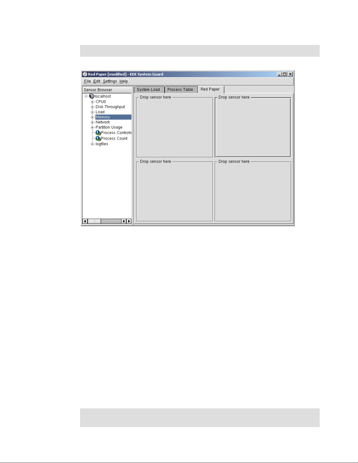
4285ch02.fm Draft Document for Review May 4, 2007 11:35 am

Note: The fastest update interval that can be defined is two seconds.

Figure 2-11 Empty worksheet

3. Fill in the sensor boxes by dragging the sensors on the left side of the window to the desired box on the right. The types of display are:

– Signal Plotter: This displays samples of one or more sensors over time. If several

sensors are displayed, the values are layered in different colors. If the display is large enough, a grid will be displayed to show the range of the plotted samples.

By default, the automatic range mode is active, so the minimum and maximum values will be set automatically. If you want fixed minimum and maximum values, you can deactivate the automatic range mode and set the values in the Scales tab from the Properties dialog window (which you access by right-clicking the graph).

– Multimeter: This displays the sensor values as a digital meter. In the Properties dialog,

you can specify a lower and upper limit. If the range is exceeded, the display is colored in the alarm color.

– BarGraph: This displays the sensor value as dancing bars. In the Properties dialog,

you can specify the minimum and maximum values of the range and a lower and upper limit. If the range is exceeded, the display is colored in the alarm color.

– Sensor Logger: This does not display any values, but logs them in a file with additional

date and time information.

For each sensor, you have to define a target log file, the time interval the sensor will be logged, and whether alarms are enabled.

4. Click File → Save to save the changes to the worksheet.

Note: When you save a work sheet, it will be saved in the user’s home directory, which may prevent other administrators from using your custom worksheets.

66 Linux Performance and Tuning Guidelines

Draft Document for Review May 4, 2007 11:35 am 4285ch02.fm

Figure 2-12 Example worksheet

Find more information about KDE System Guard at:

http://docs.kde.org/

2.3.18 Gnome System Monitor

Although not as powerful as the KDE System Guard, the Gnome desktop environment features a graphical performance analysis tool. The Gnome System Monitor can display performance-relevant system resources as graphs for visualizing possible peaks and bottlenecks. Note that all statistics are generated in real time. Long-term performance analysis should be carried out with different tools.

2.3.19 Capacity Manager

Capacity Manager, an add-on to the IBM Director system management suite for IBM Systems, is available in the ServerPlus Pack for IBM System x systems. Capacity Manager offers the possibility of long-term performance measurements across multiple systems and platforms. Apart from performance measurement, Capacity Manager enables capacity planning, offering you an estimate of future required system capacity needs. With Capacity Manager, you can export reports to HTML, XML, and GIF files that can be stored automatically on an intranet Web server. IBM Director can be used on different operating system platforms, which makes it much easier to collect and analyze data in a heterogeneous environment. Capacity Manager is discussed in detail in the redbook Tuning IBM System x Servers for Performance, SG24-5287.

To use Capacity Manager, you first must install the respective RPM package on the systems that will use its advanced features. After installing the RPM, select Capacity Manager → Monitor Activator in the IBM Director Console.

Chapter 2. Monitoring and benchmark tools 67

4285ch02.fm Draft Document for Review May 4, 2007 11:35 am

Figure 2-13 The task list in the IBM Director Console

Drag and drop the icon for Monitor Activator over a single system or a group of systems that have the Capacity Manager package installed. A window opens (Figure 2-14) in which you can select the various subsystems to be monitored over time. Capacity Manager for Linux does not yet support the full-feature set of available performance counters. System statistics are limited to a basic subset of performance parameters.

Figure 2-14 Activating performance monitors multiple systems

The Monitor Activator window shows the respective systems with their current status on the right side and the different available performance monitors at the left side. To add a new monitor, select the monitor and click On. The changes take effect shortly after the Monitor Activator window is closed. After this step, IBM Director starts collecting the requested performance metrics and stores them in a temporary location on the different systems.

To create a report of the collected data, select Capacity Manager → Report Generator (see Figure 2-13) and drag it over a single system or a group of systems for which you would like to see performance statistics. IBM Director asks whether the report should be generated right away or scheduled for later execution (Figure 2-15).

68 Linux Performance and Tuning Guidelines

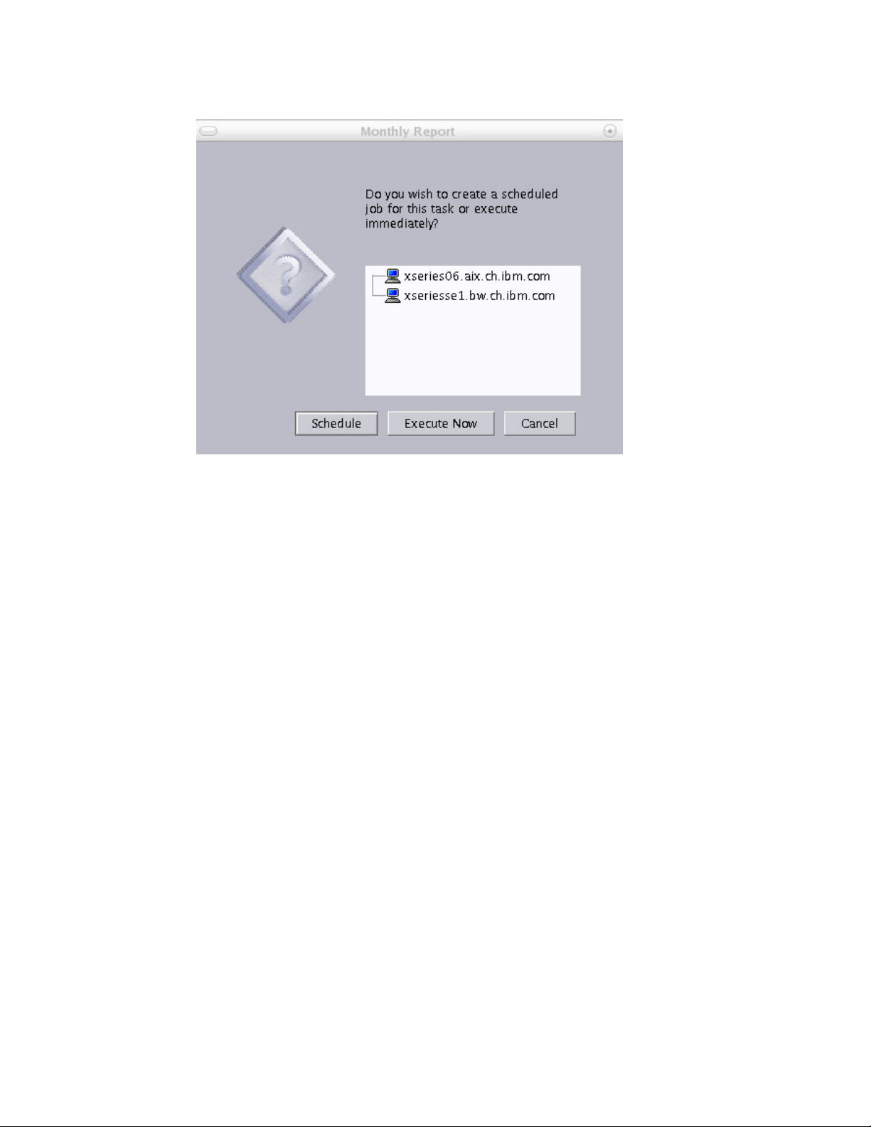
Draft Document for Review May 4, 2007 11:35 am 4285ch02.fm

Figure 2-15 Scheduling reports

In a production environment, it is a good idea to have Capacity Manager generate reports on a regular basis. Our experience is that weekly reports that are performed in off-hours over the weekend can be very valuable. An immediate execution or scheduled execution report is generated according to your choice. As soon as the report has completed, it is stored on the central IBM Director management server, where it can be viewed using the Report Viewer task. Figure 2-16 shows sample output from a monthly Capacity Manager report.

Chapter 2. Monitoring and benchmark tools 69

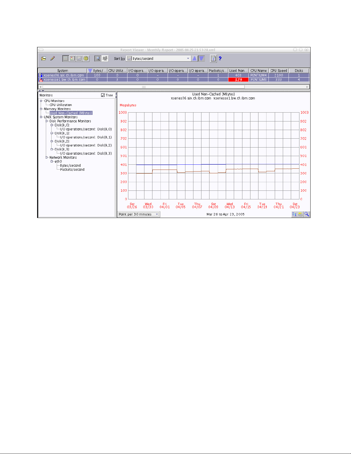
4285ch02.fm Draft Document for Review May 4, 2007 11:35 am

Figure 2-16 A sample Capacity Manager report

The Report Viewer window enables you to select the different performance counters that were collected and correlate this data to a single system or to a selection of systems.

Data acquired by Capacity Manager can be exported to an HTML or XML file to be displayed on an intranet Web server or for future analysis.

2.4 Benchmark tools

In this section, we pick up some of major benchmark tools. To measure performance it’s wise to use good benchmark tools. There are a lot of good tools available. Some of them have all or some of the following capabilities

򐂰 Load generation 򐂰 Monitor performance 򐂰 Monitor system utilization 򐂰 Reporting

A benchmark is nothing more than a model for a specific workload that may or may not be close to the workload that will finally run on a system. If a system boasts a good Linpack score it might still not be the ideal file server. You should always remember that a benchmark can not simulate the sometimes unpredictable reactions of an end-user. A benchmark will also not tell you how a file server behaves once not only the user access their data but also the backup starts up. Generally the following rules should be observed when performing a benchmark on any system:

򐂰 Use a benchmark for server workloads: Server systems boast very distinct characteristic

that make them very different from a typical desktop PC even though the IBM System x

70 Linux Performance and Tuning Guidelines

Draft Document for Review May 4, 2007 11:35 am 4285ch02.fm

platform shares many of the technologies available for desktop computers. Server benchmarks spawn multiple threads in order to utilize the SMP capabilities of the system and in order to simulate a true multi user environment. While a PC might start one web browser faster than a high-end server, the server will start a thousand web browsers faster than a PC.

򐂰 Simulate the expected workload: All benchmarks have different configuration options that

should be used to tailor the benchmark towards the workload that the system should be running in the future. Great CPU performance will be of little use if the application in the end has to rely on low disk latency.

򐂰 Isolate benchmark systems: If a system is to be tested with a benchmark it is paramount

to isolate it from any other load as good as possible. Already an open session running the top command can greatly impact the results of the benchmark.

򐂰 Average results: Even if you try to isolate the benchmark system as good as possible there

might always be unknown factors that might impact systems performance just at the time of your benchmark. It is a good practice to run any benchmark for at least three times and average the results in order to make sure that a one time event does not impact your entire analysis.

In the following sections, we’ve selected some tools based on these criteria:

򐂰 Works on Linux: Linux is the target of the benchmark

򐂰 Works on all hardware platforms: Since IBM offers three distinct hardware platforms

(assuming that the hardware technology of IBM System p and IBM System i™ are both based on the IBM POWER™ architecture) it is important to select a benchmark that may be used without big porting efforts on all architectures.

򐂰 Open source: Linux runs on several platform then the binary file may not be available if the

򐂰 Well-documented: You have to know well about the tool when you perform benchmarking.

򐂰 Actively-maintained: The old abandoned tool may not follow the recent specification and

򐂰 Widely used: You can find a lot of information about widely-used tools more easily.

򐂰 Easy to use: It’s always good thing.

򐂰 Reporting capability: Having reporting capability will greatly reduce the performance

2.4.1 LMbench

LMbench is a suite of microbenchmarks that can be used to analyze different operating system settings such as an SELinux enabled system versus a non SELinux system. The benchmarks included in LMbench measure various operating system routines such as context switching, local communications, memory bandwidth and file operations. Using LMbench is pretty straight forward as there are only three important commands to know;

򐂰 make results: The first time LMbench is run it will prompt for some details of the system

source code is not available.

The documentation will help you to be familiar with the tools. It also helps to evaluate whether the tool is suit for your needs by taking a look at the concept and design and details before you decide to use certain tool.

technology. It may produce a wrong result and lead misunderstanding.

analysis work.

configuration and what tests it should perform.

򐂰 make rerun: After the initial configuration and a first benchmark run, using the make rerun

command simply repeats the benchmark using the configuration supplied during the make results run.

Chapter 2. Monitoring and benchmark tools 71

4285ch02.fm Draft Document for Review May 4, 2007 11:35 am

򐂰 make see: Finally after a minimum of three runs the results can be viewed using the make

see command. The results will be displayed and can be copied to a spreadsheet application for further analysis or graphical representation of the data.

The LMbench benchmark can be found at http://sourceforge.net/projects/lmbench/

2.4.2 IOzone

IOzone is a file system benchmark that can be utilized to simulate a wide variety of different disk access patterns. Since the configuration possibilities of IOzone are very detailed it is possible to simulate a targeted workload profile very precisely. In essence IOzone writes one or multiple files of variable size using variable block sizes.

While IOzone offers a very comfortable automatic benchmarking mode it is usually more efficient to define the workload characteristic such as file size, I/O size and access pattern. If a file system has to be evaluated for a database workload it would be sensible to cause IOzone to create a random access pattern to a rather large file at large block sizes instead of streaming a large file with a small block size. Some of the most important options for IOzone are:

-b <output.xls> Tells IOzone to store the results in a Microsoft® Excel® compatible

spreadsheet

-C Displays output for each child process (can be used to check if all

children really run simultaneously)

-f <filename> Can be used to tell IOzone where to write the data

-i <number of test> This option is used to specify what test are to be run. You will always

have to specify -i 0 in order to write the test file for the first time. Useful tests are -i 1 for streaming reads and -i 2 for random read and random write access as well as -i 8 for a workload with mixed random access

-h Displays the onscreen help

-r Tells IOzone what record or I/O size that should be used for the tests.

The record size should be as close as possible to the record size that will be used by the targeted workload

-k <number of async I/Os>

Uses the async I/O feature of kernel 2.6 that often is used by databases such as IBM DB2®

-m Should the targeted application use multiple internal buffers then this

behavior can be simulated using the -m flag

-s <size in KB> Specifies the file size for the benchmark. For asynchronous file

systems (the default mounting option for most file systems) IOzone should be used with a file size of at least twice the systems memory in order to really measure disk performance. The size can also be specified in MB or GB using m or g respectively directly after the file size.

-+u Is an experimental switch that can be used to measure the processor

utilization during the test

72 Linux Performance and Tuning Guidelines

Draft Document for Review May 4, 2007 11:35 am 4285ch02.fm

Note: Any benchmark using files that fit into the systems memory and that are stored on asynchronous file systems will measure the memory throughput rather than the disk subsystem performance. Hence you should either mount the file system of interest with the sync option or use a file size roughly twice the size of the systems memory.

Using IOzone to measure the random read performance of a given disk subsystem mounted at /perf for a file of 10 GB size at 32KB I/O size (these characteristics could model a simple database) would look as follows:

Example 2-26 A sample IOzone command line

./iozone -b results.xls -R -i 0 -i 2 -f /perf/iozone.file -r 32 -s 10g

Finally, the obtained result can be imported into your spreadsheet application of choice and then transformed into graphs. Using a graphical output of the data might make it easier to analyze a large amount of data and to identify trends. A sample output of the example above (refer to Example 2-26) might look like the graphic displayed in Figure 2-17.

120000

100000

80000

60000

kB/sec

40000

20000

Writer Report Re-writer Report Random Read

Report

Random Write

Report

10 GB File Access at 32 KB I/O Size

Figure 2-17 A graphic produced out of the sample results of Example 2-26

If IOzone is used with file sizes that either fit into the system’s memory or cache it can also be used to gain some data about cache and memory throughput. It should however be noted that due to the file system overheads IOzone will report only 70-80% of a system’s bandwidth.

The IOzone benchmark can be found at http://www.iozone.org/

2.4.3 netperf

netperf is a performance benchmark tool especially focusing on TCP/IP networking performance. It also supports UNIX domain socket and SCTP benchmarking.

netperf is designed based on a client-server model. netserver runs on a target system and netperf runs on the client. netperf controls the netserver and passes configuration data to

Chapter 2. Monitoring and benchmark tools 73

4285ch02.fm Draft Document for Review May 4, 2007 11:35 am

netserver, generates network traffic, gets the result from netserver via a control connection which is separated from the actual benchmark traffic connection. During the benchmarking, no communication occurs on the control connection so it does not have any effect on the result. The netperf benchmark tool also has a reporting capability including a CPU utilization report. The current stable version is 2.4.3 at the time of writing.

netperf can generate several types of traffic. Basically these fall into the two categories: bulk data transfer traffic and request/response type traffic. One thing you should keep in mind is netperf uses only one socket at a time. The next version of netperf (netperf4) will fully support benchmarking for concurrent session. At this time, we can perform multiple session benchmarking as described below.

򐂰 Bulk data transfer

Bulk data transfer is most commonly measured factor when it comes to network benchmarking. The bulk data transfer is measured by the amount of data transferred in one second. It simulates large file transfer such as multimedia streaming, FTP data transfer.

򐂰 Request/response type

This simulate request/response type traffic which is measured by the number of transactions exchanged in one second. Request/response traffic type is typical for online transaction application such as web server, database server, mail server, file server which serves small or medium files and directory server. In real environment, session establishment and termination should be performed as well as data exchange. To simulate this, TCP_CRR type was introduced.

򐂰 Concurrent session

netperf does not have real support for concurrent multiple session benchmarking in the current stable version, but we can perform some benchmarking by just issuing multiple instances of netperf as follows:

for i in ‘seq 1 10‘; do netperf -t TCP_CRR -H target.example.com -i 10 -P 0 &; done

We’ll take a brief look at some useful and interesting options.

Global options:

-A Change send and receive buffer alignment on remote system

-b Burst of packet in stream test

-H <remotehost> Remote host

-t <testname> Test traffic type

TCP_STREAM Bulk data transfer benchmark

TCP_MAERTS Similar to TCP_STREAM except direction of stream is opposite.

TCP_SENDFILE Similar to TCP_STREAM except using sendfile() instead of

send(). It causes a zero-copy operation.

UDP_STREAM Same as TCP_STREAM except UDP is used.

TCP_RR Request/response type traffic benchmark

TCP_CC TCP connect/close benchmark. No request and response packet is

exchanged.

TCP_CRR Performs connect/request/response/close operation. It’s very much

like HTTP1.0/1.1 session with HTTP keepalive disabled.

UDP_RR Same as TCP_RR except UDP is used.

74 Linux Performance and Tuning Guidelines

Draft Document for Review May 4, 2007 11:35 am 4285ch02.fm

-l <testlen> Test length of benchmarking. If positive value is set, netperf perform

the benchmarking in value of benchmarking or value of type.

-c Local CPU utilization report

-C Remote CPU utilization report

Note: The report of the CPU utilization may not be accurate in some platform. Make sure if it is accurate before you perform benchmarking.

-I <conflevel><interval>

This option is used to maintain confidence of the result. The confidence level should be 99 or 95 (percent) and interval (percent) can be set as well. To keep the result a certain level of confidence, the netperf repeats the same benchmarking several times. For example,

-I 99,5 means that the result is within 5% interval (+- 2.5%) of the real result in 99 times out of 100.

-i <max><min> Number of maximum and minimum test iterations. This option limits

the number of iteration. -i 10,3 means netperf perform same benchmarking at least 3 times and at most 10 times. If the iteration exceeds the maximum value, the result would not be in the confidence level which is specified with -I option and some warning will be displayed in the result.

-s <bytes>, -S <bytes>

Changes send and receive buffer size on local, remote system. This will affect the advertised and effective window size.

testlen bytes data is exchanged for bulk data transfer

testlen seconds. If negative, it performs until

testlen transactions for request/response

Options for TCP_STREAM, TCP_MAERTS, TCP_SENDFILE, UDP_STREAM

-m <bytes>, -M <bytes>

Specifies the size of buffer passed to send(), recv() function call respectively and control the size sent and received per call.

Options for TCP_RR, TCP_CC, TCP_CRR, UDP_RR:

-r <bytes>, -R <bytes>

Specifies request, response size respectively. For example, -r 128,8129 means that netperf send 128 byte packets to the netserver

and it sends the 8129 byte packets back to netperf.

The following is an example output of netperf for TCP_CRR type benchmark.

Example 2-27 An example result of TCP_CRR benchmark

Testing with the following command line: /usr/local/bin/netperf -l 60 -H plnxsu4 -t TCP_CRR -c 100 -C 100 -i ,3 -I 95,5 -v 1 -- -r 64,1 -s 0 -S 512

TCP Connect/Request/Response TEST from 0.0.0.0 (0.0.0.0) port 0 AF_INET to plnxsu4 (10.0.0.4) port 0 AF_INET Local /Remote Socket Size Request Resp. Elapsed Trans. CPU CPU S.dem S.dem Send Recv Size Size Time Rate local remote local remote bytes bytes bytes bytes secs. per sec % % us/Tr us/Tr

Chapter 2. Monitoring and benchmark tools 75

4285ch02.fm Draft Document for Review May 4, 2007 11:35 am

16384 87380 64 1 60.00 3830.65 25.27 10.16 131.928 53.039 2048 1024

When you perform benchmarking, it’s wise to use the sample test scripts which come with netperf. By changing some variables in the scripts, you can perform your benchmarking as you like. The scripts are in the doc/examples/ directory of the netperf package.

For more details, refer to http://www.netperf.org/

2.4.4 Other useful tools

Following are some other useful benchmark tools. Keep in mind that you have to know the characteristics of the benchmark tool and choose the tools that fit your needs.

Table 2-3 Additional benchmarking tools

Tool Most useful tool function

bonnie Disk I/O and file system benchmark

http://www.textuality.com/bonnie/

bonnie++ Disk I/O and file system benchmark.

http://www.coker.com.au/bonnie++/

NetBench File server benchmark. It runs on Windows.

dbench File system benchmark. Commonly used for file server benchmark.

http://freshmeat.net/projects/dbench/

iometer Disk I/O and network benchmark

http://www.iometer.org/

ttcp Simple network benchmark

nttcp Simple network benchmark

iperf Network benchmark

http://dast.nlanr.net/projects/Iperf/

ab (Apache Bench) Simple web server benchmark. It comes with Apache HTTP server.

http://httpd.apache.org/

WebStone Web server benchmark

http://www.mindcraft.com/webstone/

Apache JMeter Used mainly web server performance benchmarking. It also support

other protocol such as SMTP, LDAP, JDBC™ etc. and it has good reporting capability.

http://jakarta.apache.org/jmeter/

fsstone, smtpstone Mail server benchmark. They come with Postfix.

http://www.postfix.org/

nhfsstone Network File System benchmark. Comes with nfs-utils package.

DirectoryMark LDAP benchmark

http://www.mindcraft.com/directorymark/

76 Linux Performance and Tuning Guidelines

Draft Document for Review May 4, 2007 11:35 am 4285ch03.fm

Chapter 3. Analyzing performance

bottlenecks

This chapter is useful for finding a performance problem that may be already affecting one of your servers. We outline a series of steps to lead you to a concrete solution that you can implement to restore the server to an acceptable performance level.

The topics that are covered in this chapter are:

򐂰 3.1, “Identifying bottlenecks” on page 78 򐂰 3.2, “CPU bottlenecks” on page 81 򐂰 3.3, “Memory bottlenecks” on page 82 򐂰 3.4, “Disk bottlenecks” on page 84 򐂰 3.5, “Network bottlenecks” on page 87

4285ch03.fm Draft Document for Review May 4, 2007 11:35 am

3.1 Identifying bottlenecks

The following steps are used as our quick tuning strategy:

1. Know your system.

2. Back up the system.

3. Monitor and analyze the system’s performance.

4. Narrow down the bottleneck and find its cause.

5. Fix the bottleneck cause by trying only one single change at a time.

6. Go back to step 3 until you are satisfied with the performance of the system.

Tip: You should document each step, especially the changes you make and their effect on performance.

3.1.1 Gathering information

Mostly likely, the only first-hand information you will have access to will be statements such as “There is a problem with the server.” It is crucial to use probing questions to clarify and document the problem. Here is a list of questions you should ask to help you get a better picture of the system.

򐂰 Can you give me a complete description of the server in question?

– Model –Age – Configuration – Peripheral equipment – Operating system version and update level

򐂰 Can you tell me

– What are the symptoms? – Describe any error messages.

Some people will have problems answering this question, but any extra information the customer can give you might enable you to find the problem. For example, the customer might say “It is really slow when I copy large files to the server.” This might indicate a network problem or a disk subsystem problem.

򐂰 Who is experiencing the problem?

Is one person, one particular group of people, or the entire organization experiencing the problem? This helps determine whether the problem exists in one particular part of the network, whether it is application-dependent, and so on. If only one user experiences the problem, then the problem might be with the user’s PC (or their imagination).

The perception clients have of the server is usually a key factor. From this point of view, performance problems may not be directly related to the server: the network path between the server and the clients can easily be the cause of the problem. This path includes network devices as well as services provided by other servers, such as domain controllers.

򐂰 Can the problem be reproduced?

All reproducible problems can be solved. If you have sufficient knowledge of the system, you should be able to narrow the problem to its root and decide which actions should be taken.

exactly what the problem is?

78 Linux Performance and Tuning Guidelines

Draft Document for Review May 4, 2007 11:35 am 4285ch03.fm

The fact that the problem can be reproduced enables you to see and understand it better. Document the sequence of actions that are necessary to reproduce the problem:

– What are the steps to reproduce the problem?

Knowing the steps may help you reproduce the same problem on a different machine under the same conditions. If this works, it gives you the opportunity to use a machine in a test environment and removes the chance of crashing the production server.

– Is it an intermittent problem?

If the problem is intermittent, the first thing to do is to gather information and find a path to move the problem in the reproducible category. The goal here is to have a scenario to make the problem happen on command.

– Does it occur at certain times of the day or certain days of the week?

This might help you determine what is causing the problem. It may occur when everyone arrives for work or returns from lunch. Look for ways to change the timing (that is, make it happen less or more often); if there are ways to do so, the problem becomes a reproducible one.

– Is it unusual?

If the problem falls into the non-reproducible category, you may conclude that it is the result of extraordinary conditions and classify it as fixed. In real life, there is a high probability that it will happen again.

A good procedure to troubleshoot a hard-to-reproduce problem is to perform general maintenance on the server: reboot, or bring the machine up to date on drivers and patches.

򐂰 When did the problem start? Was it gradual or did it occur very quickly?

If the performance issue appeared gradually, then it is likely to be a sizing issue; if it appeared overnight, then the problem could be caused by a change made to the server or peripherals.

򐂰 Have any changes been made to the server (minor or major) or are there any changes in

the way clients are using the server?

Did the customer alter something on the server or peripherals to cause the problem? Is there a log of all network changes available?

Demands could change based on business changes, which could affect demands on a servers and network systems.

򐂰 Are there any other servers or hardware components involved?

򐂰 Are any logs available?

򐂰 What is the priority of the problem? When does it have to be fixed?

– Does it have to be fixed in the next few minutes, or in days? You may have some time to

fix it; or it may already be time to operate in panic mode.

– How massive is the problem?

– What is the related cost of that problem?

Chapter 3. Analyzing performance bottlenecks 79

4285ch03.fm Draft Document for Review May 4, 2007 11:35 am

3.1.2 Analyzing the server’s performance

Important: Before taking any troubleshooting actions, back up all data and the

configuration information to prevent a partial or complete loss.

At this point, you should begin monitoring the server. The simplest way is to run monitoring tools from the server that is being analyzed. (See Chapter 2, “Monitoring and benchmark tools” on page 39, for information.)

A performance log of the server should be created during its peak time of operation (for example, 9:00 a.m. to 5:00 p.m.); it will depend on what services are being provided and on who is using these services. When creating the log, if available, the following objects should be included:

򐂰 Processor 򐂰 System 򐂰 Server work queues 򐂰 Memory 򐂰 Page file 򐂰 Physical disk 򐂰 Redirector 򐂰 Network interface

Before you begin, remember that a methodical approach to performance tuning is important. Our recommended process, which you can use for your server performance tuning process, is as follows:

1. Understand the factors affecting server performance.

2. Measure the current performance to create a performance baseline to compare with your future measurements and to identify system bottlenecks.

3. Use the monitoring tools to identify a performance bottleneck. By following the instructions in the next sections, you should be able to narrow down the bottleneck to the subsystem level.

4. Work with the component that is causing the bottleneck by performing some actions to improve server performance in response to demands.

Note: It is important to understand that the greatest gains are obtained by upgrading a component that has a bottleneck when the other components in the server have ample “power” left to sustain an elevated level of performance.

5. Measure the new performance. This helps you compare performance before and after the tuning steps.

When attempting to fix a performance problem, remember the following:

򐂰 Applications should be compiled with an appropriate optimization level to reduce the path

length.

򐂰 Take measurements before you upgrade or modify anything so that you can tell whether

the change had any effect. (That is, take baseline measurements.)

򐂰 Examine the options that involve reconfiguring existing hardware, not just those that

involve adding new hardware.

80 Linux Performance and Tuning Guidelines

Draft Document for Review May 4, 2007 11:35 am 4285ch03.fm

3.2 CPU bottlenecks

For servers whose primary role is that of an application or database server, the CPU is a critical resource and can often be a source of performance bottlenecks. It is important to note that high CPU utilization does not always mean that a CPU is busy doing work; it may, in fact, be waiting on another subsystem. When performing proper analysis, it is very important that you look at the system as a whole and at all subsystems because there may be a cascade effect within the subsystems.

Note: There is a common misconception that the CPU is the most important part of the server. This is not always the case, and servers are often overconfigured with CPU and underconfigured with disks, memory, and network subsystems. Only specific applications that are truly CPU-intensive can take advantage of today’s high-end processors.

3.2.1 Finding CPU bottlenecks

Determining bottlenecks with the CPU can be accomplished in several ways. As discussed in Chapter 2, “Monitoring and benchmark tools” on page 39, Linux has a variety of tools to help determine this; the question is: which tools to use?

One such tool is uptime. By analyzing the output from uptime, we can get a rough idea of what has been happening in the system for the past 15 minutes. For a more detailed explanation of this tool, see 2.3.3, “uptime” on page 43.

3.2.2 SMP

Example 3-1 uptime output from a CPU strapped system

18:03:16 up 1 day, 2:46, 6 users, load average: 182.53, 92.02, 37.95

Using KDE System Guard and the CPU sensors lets you view the current CPU workload.

Tip: Be careful not to add to CPU problems by running too many tools at one time. You may find that using a lot of different monitoring tools at one time may be contributing to the high CPU load.

Using top, you can see both CPU utilization and what processes are the biggest contributors to the problem (Example 2-1 on page 41). If you have set up sar, you are collecting a lot of information, some of which is CPU utilization, over a period of time. Analyzing this information can be difficult, so use isag, which can use sar output to plot a graph. Otherwise, you may wish to parse the information through a script and use a spreadsheet to plot it to see any trends in CPU utilization. You can also use sar from the command line by issuing sar -u or sar -U processornumber. To gain a broader perspective of the system and current utilization of more than just the CPU subsystem, a good tool is vmstat (2.3.2, “vmstat” on page 42).

SMP-based systems can present their own set of interesting problems that can be difficult to detect. In an SMP environment, there is the concept of bind a process to a CPU.

CPU affinity, which implies that you

The main reason this is useful is CPU cache optimization, which is achieved by keeping the same process on one CPU rather than moving between processors. When a process moves between CPUs, the cache of the new CPU must be flushed. Therefore, a process that moves between processors causes many cache flushes to occur, which means that an individual process will take longer to finish. This scenario is very hard to detect because, when

Chapter 3. Analyzing performance bottlenecks 81

4285ch03.fm Draft Document for Review May 4, 2007 11:35 am

monitoring it, the CPU load will appear to be very balanced and not necessarily peaking on any CPU. Affinity is also useful in NUMA-based systems such as the IBM System x 3950, where it is important to keep memory, cache, and CPU access local to one another.

3.2.3 Performance tuning options

The first step is to ensure that the system performance problem is being caused by the CPU and not one of the other subsystems. If the processor is the server bottleneck, then a number of actions can be taken to improve performance. These include:

򐂰 Ensure that no unnecessary programs are running in the background by using ps -ef. If

you find such programs, stop them and use cron to schedule them to run at off-peak hours.

򐂰 Identify non-critical, CPU-intensive processes by using top and modify their priority using

renice.

򐂰 In an SMP-based machine, try using taskset to bind processes to CPUs to make sure that

processes are not hopping between processors, causing cache flushes.

򐂰 Based on the running application, it may be better to scale up (bigger CPUs) than scale

out (more CPUs). This depends on whether your application was designed to effectively take advantage of more processors. For example, a single-threaded application would scale better with a faster CPU and not with more CPUs.

򐂰 General options include making sure you are using the latest drivers and firmware, as this

may affect the load they have on the CPU.

3.3 Memory bottlenecks

On a Linux system, many programs run at the same time; these programs support multiple users and some processes are more used than others. Some of these programs use a portion of memory while the rest are “sleeping.” When an application accesses cache, the performance increases because an in-memory access retrieves data, thereby eliminating the need to access slower disks.

The OS uses an algorithm to control which programs will use physical memory and which are paged out. This is transparent to user programs. Page space is a file created by the OS on a disk partition to store user programs that are not currently in use. Typically, page sizes are 4 KB or 8 KB. In Linux, the page size is defined by using the variable EXEC_PAGESIZE in the include/asm-<architecture>/param.h kernel header file. The process used to page a process out to disk is called

3.3.1 Finding memory bottlenecks

Start your analysis by listing the applications that are running on the server. Determine how much physical memory and swap each application needs to run. Figure 3-1 on page 83 shows KDE System Guard monitoring memory usage.

pageout.

82 Linux Performance and Tuning Guidelines

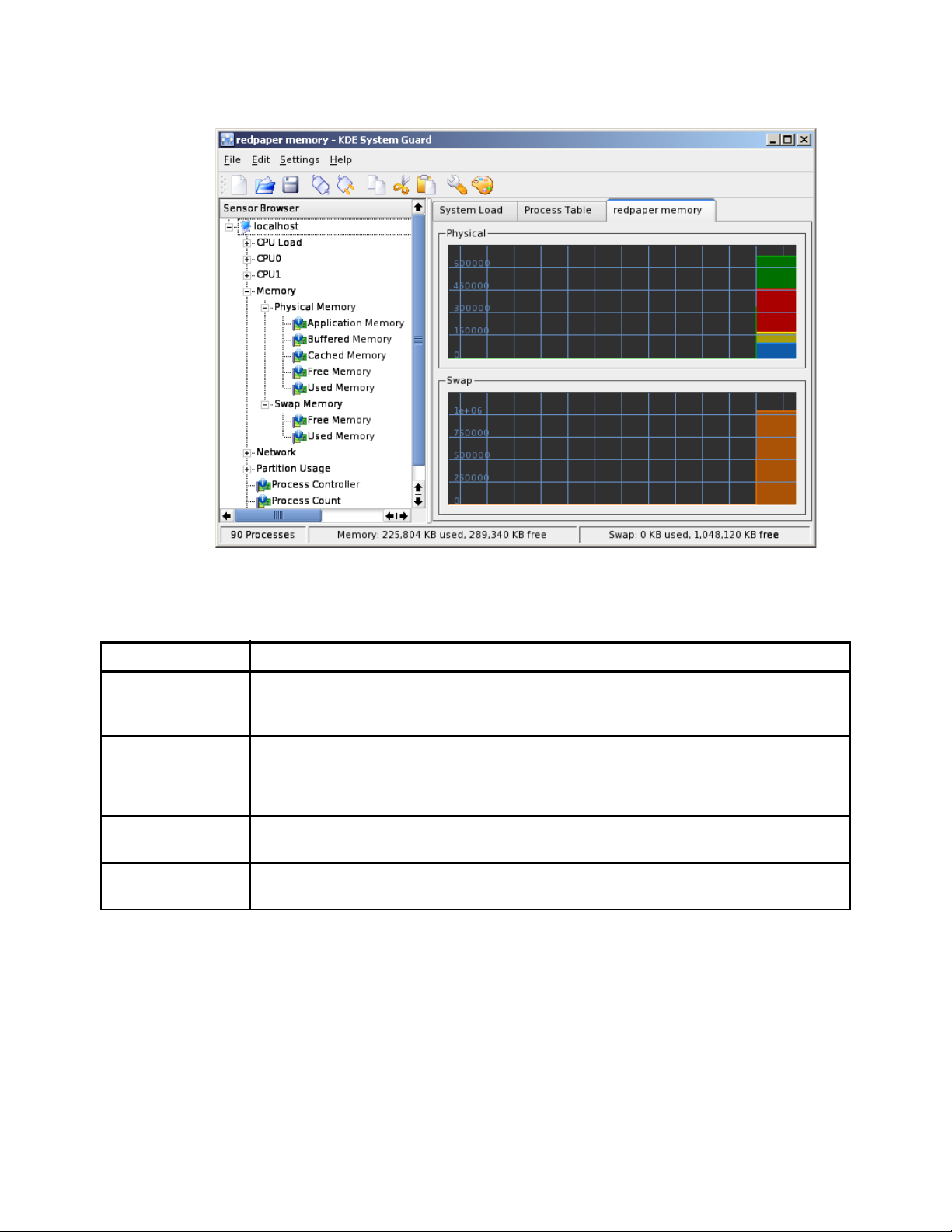
Draft Document for Review May 4, 2007 11:35 am 4285ch03.fm

Figure 3-1 KDE System Guard memory monitoring

The indicators in Table 3-1 can also help you define a problem with memory.

Table 3-1 Indicator for memory analysis

Memory indicator Analysis

Memory available This indicates how much physical memory is available for use. If, after you start your application,

this value has decreased significantly, you may have a memory leak. Check the application that is causing it and make the necessary adjustments. Use free -l -t -o for additional information.

Page faults There are two types of page faults: soft page faults, when the page is found in memory, and hard

page faults, when the page is not found in memory and must be fetched from disk. Accessing the disk will slow your application considerably. The sar -B command can provide useful information for analyzing page faults, specifically columns pgpgin/s and pgpgout/s.

File system cache This is the common memory space used by the file system cache. Use the free -l -t -o

command for additional information.

Private memory for process

This represents the memory used by each process running on the server. You can use the pmap command to see how much memory is allocated to a specific process.

Paging and swapping indicators

In Linux, as with all UNIX-based operating systems, there are differences between paging and swapping. Paging moves individual pages to swap space on the disk; swapping is a bigger operation that moves the entire address space of a process to swap space in one operation.

Swapping can have one of two causes:

򐂰 A process enters sleep mode. This usually happens because the process depends on

interactive action, as editors, shells, and data entry applications spend most of their time waiting for user input. During this time, they are inactive.

Chapter 3. Analyzing performance bottlenecks 83

4285ch03.fm Draft Document for Review May 4, 2007 11:35 am

򐂰 A process behaves poorly. Paging can be a serious performance problem when the

amount of free memory pages falls below the minimum amount specified, because the paging mechanism is not able to handle the requests for physical memory pages and the swap mechanism is called to free more pages. This significantly increases I/O to disk and will quickly degrade a server’s performance.

If your server is always paging to disk (a high page-out rate), consider adding more memory. However, for systems with a low page-out rate, it may not affect performance.

3.3.2 Performance tuning options

It you believe there is a memory bottleneck, consider performing one or more of these actions:

򐂰 Tune the swap space using bigpages, hugetlb, shared memory. 򐂰 Increase or decrease the size of pages. 򐂰 Improve the handling of active and inactive memory. 򐂰 Adjust the page-out rate. 򐂰 Limit the resources used for each user on the server. 򐂰 Stop the services that are not needed, as discussed in “Daemons” on page 97. 򐂰 Add memory.

3.4 Disk bottlenecks

The disk subsystem is often the most important aspect of server performance and is usually the most common bottleneck. However, problems can be hidden by other factors, such as lack of memory. Applications are considered to be I/O-bound when CPU cycles are wasted simply waiting for I/O tasks to finish.

The most common disk bottleneck is having too few disks. Most disk configurations are based on capacity requirements, not performance. The least expensive solution is to purchase the smallest number of the largest-capacity disks possible. However, this places more user data on each disk, causing greater I/O rates to the physical disk and allowing disk bottlenecks to occur.

The second most common problem is having too many logical disks on the same array. This increases seek time and significantly lowers performance.

The disk subsystem is discussed in 4.6, “Tuning the disk subsystem” on page 113.

3.4.1 Finding disk bottlenecks

A server exhibiting the following symptoms may be suffering from a disk bottleneck (or a hidden memory problem):

򐂰 Slow disks will result in:

– Memory buffers filling with write data (or waiting for read data), which will delay all

requests because free memory buffers are unavailable for write requests (or the response is waiting for read data in the disk queue)

– Insufficient memory, as in the case of not enough memory buffers for network requests,

will cause synchronous disk I/O

򐂰 Disk utilization, controller utilization, or both will typically be very high.

򐂰 Most LAN transfers will happen only after disk I/O has completed, causing very long

response times and low network utilization.

84 Linux Performance and Tuning Guidelines

Draft Document for Review May 4, 2007 11:35 am 4285ch03.fm

򐂰 Disk I/O can take a relatively long time and disk queues will become full, so the CPUs will

be idle or have low utilization because they wait long periods of time before processing the next request.

The disk subsystem is perhaps the most challenging subsystem to properly configure. Besides looking at raw disk interface speed and disk capacity, it is key to also understand the workload: Is disk access random or sequential? Is there large I/O or small I/O? Answering these questions provides the necessary information to make sure the disk subsystem is adequately tuned.

Disk manufacturers tend to showcase the upper limits of their drive technology’s throughput. However, taking the time to understand the throughput of your workload will help you understand what true expectations to have of your underlying disk subsystem.

Table 3-2 Exercise showing true throughput for 8 KB I/Os for different drive speeds

Disk speed Latency Seek

time

15 000 RPM 2.0 ms 3.8 ms 6.8 ms 147 1.15 MBps

10 000 RPM 3.0 ms 4.9 ms 8.9 ms 112 900 KBps

Total random access time

I/Os per

second per disk

Throughput given 8 KB I/O

7 200 RPM 4.2 ms 9 ms 13.2 ms 75 600 KBps

a. Assuming that the handling of the command + data transfer < 1 ms, total random access time = latency + seek time + 1 ms. b. Calculated as 1/total random access time.

Random read/write workloads usually require several disks to scale. The bus bandwidths of SCSI or Fibre Channel are of lesser concern. Larger databases with random access workload will benefit from having more disks. Larger SMP servers will scale better with more disks. Given the I/O profile of 70% reads and 30% writes of the average commercial workload, a RAID-10 implementation will perform 50% to 60% better than a RAID-5.

Sequential workloads tend to stress the bus bandwidth of disk subsystems. Pay special attention to the number of SCSI buses and Fibre Channel controllers when maximum throughput is desired. Given the same number of drives in an array, RAID-10, RAID-0, and RAID-5 all have similar streaming read and write throughput.

There are two ways to approach disk bottleneck analysis: real-time monitoring and tracing.

򐂰 Real-time monitoring must be done while the problem is occurring. This may not be

practical in cases where system workload is dynamic and the problem is not repeatable. However, if the problem is repeatable, this method is flexible because of the ability to add objects and counters as the problem becomes well understood.

򐂰 Tracing is the collecting of performance data over time to diagnose a problem. This is a

good way to perform remote performance analysis. Some of the drawbacks include the potential for having to analyze large files when performance problems are not repeatable, and the potential for not having all key objects and parameters in the trace and having to wait for the next time the problem occurs for the additional data.

vmstat command

One way to track disk usage on a Linux system is by using the vmstat tool. The columns of interest in vmstat with respect to I/O are the bi and bo fields. These fields monitor the movement of blocks in and out of the disk subsystem. Having a baseline is key to being able to identify any changes over time.

Chapter 3. Analyzing performance bottlenecks 85

4285ch03.fm Draft Document for Review May 4, 2007 11:35 am

Example 3-2 vmstat output

[root@x232 root]# vmstat 2 r b swpd free buff cache si so bi bo in cs us sy id wa 2 1 0 9004 47196 1141672 0 0 0 950 149 74 87 13 0 0 0 2 0 9672 47224 1140924 0 0 12 42392 189 65 88 10 0 1 0 2 0 9276 47224 1141308 0 0 448 0 144 28 0 0 0 100 0 2 0 9160 47224 1141424 0 0 448 1764 149 66 0 1 0 99 0 2 0 9272 47224 1141280 0 0 448 60 155 46 0 1 0 99 0 2 0 9180 47228 1141360 0 0 6208 10730 425 413 0 3 0 97 1 0 0 9200 47228 1141340 0 0 11200 6 631 737 0 6 0 94 1 0 0 9756 47228 1140784 0 0 12224 3632 684 763 0 11 0 89 0 2 0 9448 47228 1141092 0 0 5824 25328 403 373 0 3 0 97 0 2 0 9740 47228 1140832 0 0 640 0 159 31 0 0 0 100

iostat command

Performance problems can be encountered when too many files are opened, being read and written to, then closed repeatedly. This could become apparent as seek times (the time it takes to move to the exact track where the data is stored) start to increase. Using the iostat tool, you can monitor the I/O device loading in real time. Different options enable you to drill down even farther to gather the necessary data.

Example 3-3 shows a potential I/O bottleneck on the device /dev/sdb1. This output shows average wait times (await) of about 2.7 seconds and service times (svctm) of 270 ms.

Example 3-3 Sample of an I/O bottleneck as shown with iostat 2 -x /dev/sdb1

[root@x232 root]# iostat 2 -x /dev/sdb1

avg-cpu: %user %nice %sys %idle

11.50 0.00 2.00 86.50

Device: rrqm/s wrqm/s r/s w/s rsec/s wsec/s rkB/s wkB/s avgrq-sz avgqu-sz await svctm %util /dev/sdb1 441.00 3030.00 7.00 30.50 3584.00 24480.00 1792.00 12240.00 748.37

101.70 2717.33 266.67 100.00

avg-cpu: %user %nice %sys %idle

10.50 0.00 1.00 88.50

Device: rrqm/s wrqm/s r/s w/s rsec/s wsec/s rkB/s wkB/s avgrq-sz avgqu-sz await svctm %util /dev/sdb1 441.00 3030.00 7.00 30.00 3584.00 24480.00 1792.00 12240.00 758.49

101.65 2739.19 270.27 100.00

avg-cpu: %user %nice %sys %idle

10.95 0.00 1.00 88.06

Device: rrqm/s wrqm/s r/s w/s rsec/s wsec/s rkB/s wkB/s avgrq-sz avgqu-sz await svctm %util /dev/sdb1 438.81 3165.67 6.97 30.35 3566.17 25576.12 1783.08 12788.06 781.01

101.69 2728.00 268.00 100.00

For a more detailed explanation of the fields, see the man page for iostat(1).

86 Linux Performance and Tuning Guidelines

IBM REDP-4285-00 User Manual

Specifications and Main Features

Frequently Asked Questions

User Manual

Front cover

Contents

Notices

Trademarks

Preface

How this Redpaper is structured

The team that wrote this Redpaper

Become a published author

Comments welcome

1.1 Linux process management

1.1.1 What is a process?

1.1.2 Lifecycle of a process

1.1.3 Thread

1.1.4 Process priority and nice level

1.1.5 Context switching

1.1.6 Interrupt handling

1.1.7 Process state

1.1.8 Process memory segments

1.1.9 Linux CPU scheduler

1.2 Linux memory architecture

1.2.1 Physical and virtual memory

1.2.2 Virtual memory manager

1.3 Linux file systems

1.3.1 Virtual file system

1.3.2 Journaling

1.3.3 Ext2

1.3.4 Ext3

1.3.5 ReiserFS

1.3.6 Journal File System

1.3.7 XFS

1.4 Disk I/O subsystem

1.4.1 I/O subsystem architecture

1.4.2 Cache

1.4.3 Block layer

1.4.4 I/O device driver

1.4.5 RAID and Storage system

1.5 Network subsystem

1.5.1 Networking implementation

1.5.2 TCP/IP

1.5.3 Offload

1.5.4 Bonding module

1.6 Understanding Linux performance metrics

1.6.1 Processor metrics

1.6.2 Memory metrics

1.6.3 Network interface metrics

1.6.4 Block device metrics

Chapter 2. Monitoring and benchmark tools

2.1 Introduction

2.2 Overview of tool function

2.3 Monitoring tools

2.3.1 top

2.3.2 vmstat

2.3.3 uptime

2.3.4 ps and pstree

2.3.5 free

2.3.6 iostat

2.3.7 sar

2.3.8 mpstat

2.3.9 numastat

2.3.10 pmap

2.3.11 netstat

2.3.12 iptraf

2.3.13 tcpdump / ethereal

2.3.14 nmon

2.3.15 strace

2.3.16 Proc file system

2.3.17 KDE System Guard

2.3.18 Gnome System Monitor

2.3.19 Capacity Manager

2.4 Benchmark tools

2.4.1 LMbench

2.4.2 IOzone

2.4.3 netperf

2.4.4 Other useful tools

3.1 Identifying bottlenecks

3.1.1 Gathering information