

Page 1

User's Guide
WHSl HEWLETT»
mL'HM PACKARD
O
CO
pLi
Page 2
aplet views
aplet library -
Home -
for entering
Alpha shift
shift key
(turquoise)
HEWLETT A
'Hm PACKARD
LI VIEWS NOTE SKETCH
_____
1 1 MODES ASIN ACOS ATAN x-1
1 1
1 1 ANSWER CHARS EEX
BIE^
a...z LIST
CLEAR NOTEPAD SPACE K LN
OFF PROGRAM
021 ■■ I
CANCEL
a a
7 ■ 8 ■ g ■ /
MATRIX [
1 ■ 2 I 3
G H
5 ■ 6 ■ ^
a
ABS
B,
) LOG
___
]_ 10^
U
B38G
D-
'll—
^0
-fi
X2
The {{ok}} menu-key
label (when present in
the display) acts the
same as the | enter]
key.
Key Conventions-Examples:
■ [ANSWER] Means press the shift key followed by the | enter] key.
|a...z|A Means press the Alpha-shift key followed by the | home | key.
Page 3

HP 38G Graphing Calculator
User’s Guide
HEWLETT®
PACKARD
HP Part No. FI 200-90013
Printed in Singapore
Page 4

Notice
This manual and any examples contained herein are provided “as is” and are
subject to change without notice. Hewlett-Packard Company makes no warranty
of any kind with regard to this manual, including, but not limited to, the implied
warranties of merchantability and fitness for a particular purpose. Hewlett-Packard
Co. shall not be liable for any eiTors or for incidental or consequential damages in
connection with the furnishing, performance, or use of this manual or the examples
herein.
© Copyright Hewlett-Packard Company 1995. All rights reserved. Reproduction,
adaptation, or translation of this manual is prohibited without prior written
permission of Hewlett-Packard Company, except as allowed under the copyright
laws.
The programs that control this product are copyrighted and all rights are reserved.
Reproduction, adaptation, or translation of those programs without prior written
permission of Hewlett-Packard Co. is also prohibited.
Hewlett-Packard Co.
Australian Calculator Operation
347, Burwood Highway
Burwood East
Victoria 3151
Australia
Acknowledgments
Hewlett-Packard gratefully acknowledges the members of the Education Advisory
Committee (Walter Bitz, Tom Dick, Mark Howell, Alice Kaseberg, Jim McManus,
Carla Randall, Alison Warr, and Wade White) for their assistance in the
development of this product.
Edition History
Edition 2
...............
.January 1998
Page 5

Contents
Getting Started
Starting Out...........................................................................1-1
The Keyboard
The Display.............................................................................1-6
Display Modes
Using Input Forms
Home History......................................................................1-9
Menu Lists........................................................................ 1-10
Aplets and Their Views.......................................................1-11
Aplets.................................................................................1-11
Views..................................................................................1-12
Exploring an Aplet View by View
Catalogs and Editors...........................................................1-16
Storing and Recalling Variables
Notes and Sketches
Note View and Sketch View
The Notepad......................................................................1-23
Managing Aplets....................................................................1 -25
Sending and Receiving Aplets
Mathematical Calculations
How to Do Calculations........................................................2-1
Entering Expressions.........................................................2-1
Complex Numbers..............................................................2-4
Clearing Numbers..............................................................2-4
Using Previous Results.......................................................2-4
Storing in Variables...............................................................2-6
The VAR Menu......................................................................2-7
Symbolic Calculations
Using Math Functions.........................................................2-12
The MATH Menu.............................................................2-12
The Math Functions by Category...................................2-13
........................................................................
....................................................................
.............................................................
...................................
........................................
..............................................................
............................................
............................................
.........................................................
1-2
1-7
1-8
1 -14
1-17
1-18
1-18
1-27
2-10
Contents-1
Page 6

Plotting and Exploring Functions
Defining a Problem
Select an Aplet
Define an Expression (Symbolic View)............................3-2
Evaluating Expressions
Examples: Defining Expressions
Plotting....................................................................................3-7
Plot the Expression (Plot View)
Examples: Plotting
Exploring the Plot
Tracing
..............................................................................
Zooming.............................................................................3-13
Other Views for Scaling and Splitting the Graph
Setting Up the Plot (Plot Setup)
Interactive Root-Finding
Examples: Root-Finding with Plots
Using a Table of Numbers
Display a Table of Numbers (Numeric View)
Exploring the Table of Numbers
Setting Up the Table (Numeric Setup)
Building Your Own Table of Numbers..........................3-26
More Examples
...............................................................
....................................................................
.....................................................
......................................
........................................
.............................................................
...............................................................
..........
.........................................
.................................................
...............................
..................................................
...............
....................................
...........................
....................................................................
Solve
Solving Equations..................................................................4-2
Define the Equation
Solve for the Unknown Variable
Plotting the Equation
Interpreting Results...............................................................4-7
Plotting to Find Guesses........................................................4-8
About Variables...................................................................4-11
...........................................................
......................................
............................................................
3-1
3-2
3-5
3-6
3-7
3-8
3-11
3-12
3-16
3-18
3-19
3-21
3-23
3-23
3-24
3-25
3-28
4-2
4-4
4-6
Contents-2
Page 7

Statistics
Example: Finding a Linear Equation to Fit Data
Entering Statistical Data.......................................................5-5
One-Variable Data
Two-Variable Data.............................................................5-9
Managing Statistical Data
Analyzing the Data
Defining a Regression Model (2VAR)............................5-14
Computing Statistics (IVAR and 2VAR)
Plotting..................................................................................5-19
Plot Types..........................................................................5-20
Fitting a Curve to 2VAR Data........................................5-21
Regression Coefficients
Plot Settings
Trouble-shooting
Exploring the Plot................................................................5-23
Calculating Predicted Values..........................................5-24
.............................................................
...............................................
..............................................................
...................................................
......................................................................
..............................................................
..............
....................
Using Matrices
Creating and Storing Matrices
Matrix Arithmetic..................................................................6-6
Solving Systems of Linear Equations
Matrix Functions....................................................................6-9
Examples...........................................................................6-13
............................................
...............................
5-2
5-6
5-12
5-14
5-16
5-21
5-22
5-22
6-1
6-8
Using Lists
Creating and Storing Lists
List Functions.........................................................................7-4
Finding Statistical Values for List Elements
...................................................
...................
7-1
7-7
Contents-3
Page 8

Programming
The Contents of a Program...............................................8-1
Structured Programming
Using the Program Catalog..................................................8-1
Programming Commands
Aplet Commands..............................................................8-10
Branch Commands..........................................................8-11
Drawing Commands
Graphic Commands.........................................................8-15
Loop Commands
Matrix Commands
Print Commands
Prompt Commands
Stat-One and Stat-two Commands.................................8-25
Storing and Retrieving Variables in Programs
The Variable Menu
Plot-View Variables
Symbolic-View Variables
Numeric-View Variables
Note Variables
Sketch Variables...............................................................8-39
Menu Maps of the VAR menu.............................................840
Home Variables................................................................8-40
Function Variables...........................................................8-40
Parametric Variables
Polar Vciriables................................................................8-41
Sequence Variables............................................................842
Solve Variables...................................................................842
Statistics Variables
..................................................................
.................................................
....................................................
........................................................
..............................................................
...........................................................
..............................................................
.........................................................
................
..........................................................
.........................................................
................................................
.................................................
......................................................
............................................................
8-1
8-9
8-13
8-17
8-18
8-20
8-21
8-26
8-26
8-28
8-35
8-37
8-39
8-41
843
Reference Information
Regulatory Information........................................................9-1
Limited One-Year Warranty
Service
......................................................................................
Batteries..................................................................................9-7
Resetting the HP 38G............................................................9-8
Memory Specifications..........................................................9-8
Glossary..................................................................................9-9
Selected Status Messages....................................................9-11
...............................................
Content84
9-3
94
Page 9
Getting Started
Read this chapter first! It will get you started using your
HP 38G, from turning it on to running aplets.
Starting Out
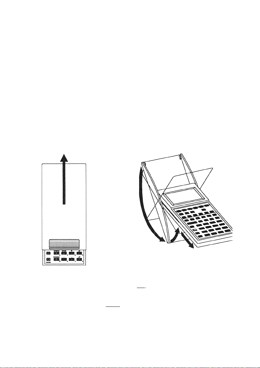
The Cover The protective cover swivels to provide a base for the
calculator. Be sure to protect the display by replacing the
cover before transporting the calculator. Slide the cover
gently so as not to hit the keys.
First push the
cover away
from you until it
catches.
ON/CANCEL When the calculator is on, the |on| key cancels the current
operation.
OFF
Pressing ■ I ON I (that is, ■ [OFF]) turns the calculator off.
Then swivel the cover to the
back and slide it towards you.
Getting Started 1-1
Page 10

Demo
To see a demonstration of the HP 38G's features, type DEMO
into the edit line in Home. (Press | home | |a...z|D |a...z|E
|A...z|M |A...z|0 I ENTER|.) To Stop the demo, press any key.
Home
Power
Home is the calculator’s home base. If you want to do
calculations, or you want to quit the current activity (such as
an aplet, a program, or an editor), press | home |.
To save power, the calculator turns itself off after several
minutes of inactivity. All stored and displayed information are
saved.
If you see the ((*)) annunciator or the Low Bat message,
then the calculator needs fresh batteries. See chapter 9.
The Keyboard
Shifted The ■ (shift) key is a shifted keystroke that accesses the
Keystrokes operation printed in turquoise above a key. For instance, to
® access the Modes screen, press ■, then | home |. (You do not
need to hold down the ■ .) This is depicted in this manual as
“press ■[MODES] ."
To cancel a shift, press ■ again.
Alpha Shift The alphabetic keys are also shifted keystrokes. For instance,
l^ -^l to type z, press | A...Z | (T|. (The letters are printed in light
green to the lower right of each key.)
To cancel Alpha, press | A...Z | again.
• For a lowercase letter, press ■ | A...Z |.
• For a string of letters, hold down | A...Z | while typing.
1-2 Getting Started
Page 11

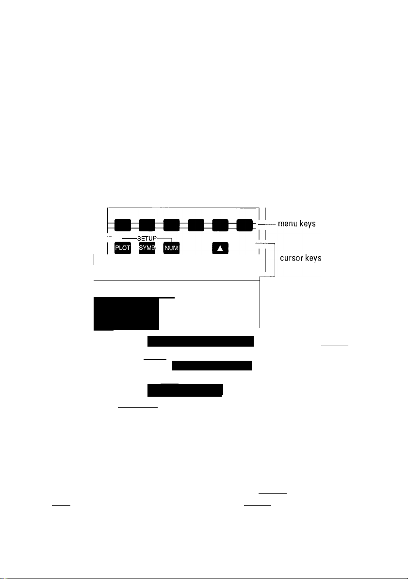
Menu Keys You can press fuBl to see this screen;
menu labels
mm
menu keys
« The top-row keys are called menu keys because their
meanings depend on the context—that’s why their tops
are blank.
• The bottom line of the display shows the labels for the
menu keys’ current meanings, {{save}} is the label for the
first menu key in this picture. “Press {{save}}’’ means to
press the leftmost top-row key.
Parametric
Polar
Sequence
Solve
Math Keys
Home (press | home |) is the place to do calculations.
• Keyboard keys. The most common arithmetic operations
are on the keyboard, such as the arithmetic (like (T)) and
trigonometric (like |sin|) functions. Press | enter | to
complete the operation : |^] 256 | enter | displays 16 .
P256
16
Getting Started 1-3
Page 12

MATH menu. The | math | menu is a comprehensive menu
list of math operations that do not appear on the keyboard.
It also includes categories for all other functions and
programmable commands. The functions are grouped by
category, ranging in alphabetical order from Calculus to
Trigonometry.
Re.3l C CEILING
Stat-Tyo
Symbolic
—
Tests ? FNROOT »
BDBSISiaiSI iHamBM
DEG+RFID
FLOOR
The arrow keys scroll through the list (Q. ®) ^^d move
from the category list to the item list (0, Q).
Press {{cancl}} to cancel the MATH menu.
Pressing {{CMDS}} displays the list of Program Commands.
Pressing {{CONS}} displays the list of Program Constants.
Pressing {{MTH}} displays the list of Math Functions.
1-4 Getting Started
Page 13

Keys for Entry
and Editing
Key
(CANCEL)
Meanine
Pressing |ON| while the calculator is on
cancels the current operation. Pressing ■
first turns the calculator off.
■ (shift)
1 HOME 1
[M]
1 ENTER 1 Enters an input or executes an operation. In
Q
[EEX] Enters an exponent of 10. To enter 5x10^
1 x,T,e 1
[MD
■ [CLEAR]
Accesses the function printed in turquoise
color above a key.
Home base for calculations.
Alphabetic entry—press before a letter key.
calculations, 1 enter 1 acts like “=“ When
{{OK}} is present as a menu key, | enter] acts
the same as {{OK}}.
Starts a negative number. To enter -5,
press 5.
you press 5 ■ [EEX] 9. This appears as
5E9 or, after pressing | enter],
5000000000.
Independent variable key. Types X, T, 0, or
N into the display, depending on the
current context.
Delete key. Backspaces if at the end of the
line.
Clear key. Clears all data on the screen
except settings, which return to their default
values.
0 B 0
a
■ [CHARS] Displays all available characters. To type
Inactive Keys If you press a key that does not operate in the current context,
a warning symbol like this A appears. There is no beep.
Cursor-movement (navigation) keys. Press
■ first to move far.
one, highlight it and press {{OK}}.
Getting Started 1-5
Page 14

The Display
To adjust the contrast
The Parts of the Display
Annunciators
Simultaneously press
decrease) the contrast
6*3
history
edit line
B
Mmsm
a
((•))
i
A T
RAD
GRD
DEG
8/5
:
17894
Shift in effect for next keystroke. To cancel,
press ■ again.
Alpha in effect for next keystroke. To cancel,
press 1 A...Z 1 again.
Low battery power. See chapter 9.
Busy.
Data is being transferred via infrared or cable.
There is more history in the Home display.
Scroll up or down to see it.
Radians angle mode is set for Home.
Grads angle mode is set for Home.
Degrees angle mode is set for Home.
and 0 (or0) to increase (or
18
1.6
_ menu-key
labels
To clear the display
• Press
• Press ■
history.
1-6 Getting Started
to clear the edit line.
[CLEAR] to clear the edit line and the display
Page 15

Display Modes
You can set the Home modes in ^ [MODES]. You make
your selections using an input form. To fill out an input form,
see “Using Input Forms,” after this table. The Decimal Mark
setting affects all aplets, as well as Home.
When you are done setting MODES, press | home | to return to
the Home screen.
[MODES]
Setting
Angle
Measure
Number
Format
Decimal
Mark
Title
Options
Angle values are:
Degrees. 360 degrees in a circle.
Radians. 2Tr radians in a circle.
Grads. 400 grads in a circle.
Standard. Full-precision display.
Fbted. Displays results rounded to a number of
decimal places. Example ; 123.456789 becomes
123.4568 in Fixed 4 format.
Scientific. Displays result with an exponent,
one digit to the left of the decimal point, and
the specified number of decimal places.
Example: 123.456789 becomes 1.23E2 in
Scientific 2 format.
Engineering. Displays result with an exponent
that is a multiple of 3, and the specified number
of significant digits beyond the first one.
Example: 123.456E7 becomes 1.23E9 in
Engineering 2 format.
Fraction. Displays results as fractions based on
the specified number of decimal places for
precision. Examples: 123.456789 becomes 123
in Fraction 2 format, and .333 becomes 1/3 and
29/1000 becomes 2/69.
Dot or Comma. Displays a number as 12456.98
(Dot mode) or as 12456,98 (Comma mode).
Dot mode uses commas to separate elements in
lists and matrices, and to separate function
arguments. Comma mode uses periods as
separators in these contexts.
Customizes the title in the Home screen.
Getting Started 1-7
Page 16

To display
fractions
Set Fraction mode to display future results as fractions,
1. Press ■ [MODES], then press 0 to select number
FORMAT.
2. Press {{CHOOS}}, highlight Fraction, and press {{OK}}.
3. Press and enter a number for the precision of the
fraction. The precision number determines how many
digits appear in the denominator. Press | enter |.
4. Press I HOME I to display Home.
To convert a
result to a
fraction
1. Set Fraction mode (as in the previous procedure).
2. In Home, press 0 to highlight the number in the history
display that you want to convert.
3. Press ((COPY)) lENTERj.
Using Input Forms
An input form shows several fields of information for you to
examine and specify. After highlighting the field to edit, you
can enter or edit a number (or expression). You can also
select options from a list ({{CHOOS}}). Some input forms
include items to check ({{/CHK}}).
ANGLE MEASURE: [^PfiifeEH
NUMRER FORMAT; Standard
DECIMAL MARK; Dot < . >
TITLE; HOME
CHOOSE ANGLE MEASURE
Example: Change the Angle Measure.
Setting Modes
1. Press ■ {MODES} to open the MODES input form.
2. The cursor (highlight) should be on the first line, ANGLE
MEASURE. Press {{CHOOS}} to display a list of choices.
Highlight Degrees, Radians, or Grads and press
{{OK}}.
HOME MOPES I
3. When done, press | home | to return to Home.
1-8 Getting Started
Page 17

Hint
Whenever an input form has a list of choices for a field,
you can press (T) to cycle through them instead of using
{{CHOOS}}.
To reset values To reset the original, default value in an input form, press
I DEL |. To reset all values in the form, press ■ [CLEAR].
Home History
The Home display (press | home |) shows up to four lines of
history : the most recent input and output. Older lines scroll
off the top of the display but are retained in memory; press
m to view them. Note that these examples are in Standard
display mode.
input —
last input-
edit
line
T2
— 5*77+4
When you highlight a previous input or result (pressing [Tl)
the {{COPY}} and {{show}} menu labels appear. Pressing
{{COPY}} copies the highlighted value to the edit line.
HDME
1.41421356237
HOME
-result
■last
result
T2
1.41421356
5*77+1.414213562374
To copy a Highlight the line (press |T|) and press {{COPY}}. The number
previous line (or expression) is copied into the edit line.
To repeat a To repeat the very last line, just press ( enter |. Otherwise,
previous line highlight the line (press |T1) first, and then press | enter). The
highlighted expression or number is re-entered.
Getting Started 1-9
Page 18

To re-use a Press ■ [ANSWER] (last answer) to put the last result from
previous result Home into an expression. Ans is a variable that is updated
each time you press [ enter |.
Example See how [ANSWER] retrieves and reuses the last result (50),
and I ENTER I updates Ans (from 50 to 75 to 100).
To display the
full number
Menu Lists
50 I ENTER I
25QH [ANSWER]
25+flns
1 enter! I enter!
You can use the last result as the first expression in the edit
line without pressing ■ [ANSWER]. Pressing 0, 0, or
[7], (or other operators that require a preceding argument)
automatically enters Ans before the operator.
You can reuse any other expression or value in the Home
display by highlighting the expression (using the arrow keys),
then pressing {{copy}}.
If a number or expression is too long to appear on one line,
then highlight it (press 0) and press {{SHOW}}. If it is still too
long, press [0 to see more. When done, press {{OK}}.
A menu offers you a choice of items. The menu labels across
the bottom of some displays are one kind of menu. A menu
list, which appears in one or two columns, is another kind.
FUNCTIONS
Plot-Table
Overlay Plot
fiuto Scale
Decimal
Stat-Two DEG-»RflD
Symbolic
Tests V FNROOT w
CEILIHG
FLOOR
100
50
75
• The ▼ arrow in the display means more items below.
• The A arrow in the display means more items above.
1-10 Getting Started
Page 19

To search a
menu list
® Press @ or 0 to scroll through the list. If you press
■ Q or ■ [^, you’ll go all the way to the end or the
beginning of the list. Highlight the item you want to select,
then press {{OK}} (or | enter |).
• If there are two columns, the left column shows general
categories and the right column shows specific contents.
Highlight the category on the left, then highlight the item
on the right. The list on the right changes when a different
category is highlighted. Press {{OK}} or [ enter |.
• To speed-search a list, type the first letter of the word. For
example, to find the Matrix category in |math|, press M
(the g key).
• To go up a page, you can press ■ Q- To go down a page,
press ■ .
To cancel a
menu list
Press CANCEL or {{CANCL}}. This cancels the current
operation.
Aplets and Their Views
Aplets
The HP 38G provides built-in applications to solve specific
kinds of math problems. These little applications, or aplets,
are accessed from the Library (|lib|).
The library lists (and manages) all the aplets in the
calculator, whether they came with the calculator or were
added later.
There are six types of math aplets built into the HP 38G :
Function
Parametric
Polar
• Real-valued, rectangular function y in terms of x. Example:
y = 2x-e3.
• Parametric functions x and y in terms of t. Example: x =
cos(0 and y = sin(f).
• Polar function r in terms of an angle 8.
Example: r = 2cos(40 ).
Getting Started 1-11
Page 20
Sequence ® Sequence function i/in terms of n, or in terms of previous
terms in the sequence, such asUn~i and Example:
i/i = 0, f/2 = l,and a = +
Solve ® Finding the roots of an equation.
Example: x + 1 = -x-2.
Statistics e Analysis of one-variable (x) or two-variable (x and y)
statistical data.
Views
An aplet is represented in different ways. These views
compose an aplet problem and its solution. Here are
illustrations of three major and six supporting aplet views.
SYMB
Symbolic view. The defining
equation(s) (in most aplets).
The equation contains a
symbolic expression.
FUNCTION SVMtDLIC
^F10f>SIH<X)
F3<:x)=
F4<X>=
F5<X>= ¥
PLOT
INUM!
Plot view. The graph of the
function(s).
Numeric view. Sampled
values of the function(s).
1-12 Getting Started
K: 0 FICH
.0ЦЦBЗЭH
.SRSSSOS
.H7RH353
0
BHoai
: <! i8h:ih
FI
Page 21
■ [SETUPSYMB]
Symbolic Setup (■ |symb|).
Sets parameters for the
symbolic expression.
FUMCTIDN SVMeOUC SETUP
ANGLE MEASURE:
CHMSE ANGLE MEASURE
Radian
■ [SETUPPLOT]
■ [SETUP-
NUM]
■ [VIEWS]
Plot-Table
I [NOTE]
I [SKETCH]
Plot Setup (■ I PLOT I). Sets
parameters to plot a graph.
Numeric Setup (■ | numQ.
Sets parameters for building
a table of numeric values.
Split Screen view. Two
views side by side.
Note view. Text to
supplement an aplet.
Sketch view. Pictures to
supplement an aplet.
^^^FONCIiDN PLDT
KRNG: IMÜJiii
VRNG; -3. 1
KTICK! 1 TTICK: 1
RES: Faster
ENTER MINIMUM HDRIZDNTAL VALUE
^^PUHCTIUN NUMERIC SETUP
NUMSTART: ISHPBMBIlga
NUMSTEP: . 1
NUMivPE: fiutomatic
NUMSBUM: 4
■ 6.5
3.2
ENTER STARTING VALUE FUR TAiLE
Changing
Views
BannaHQi
BrjfaiinM
Each view is a separate “environment." To change the view,
press another view key. To change to Home, press | home |.
You do not explicitly “close” the current view, you just enter
another one-like passing from one room into another in a
house.
Getting Started 1-13
Page 22
Canceling To cancel an operation within a view, press |on| (the
Operations CANCEL key). Pressing CANCEL will cancel pending
operations, but will not change the view.
Exploring an Aplet View by View
Example Use the Function aplet to explore the real function
y = sin(l/x)
using the Symbolic, Plot, and Numeric views. All the
information you enter is automatically saved
1. Open the Function aplet. Press
|lib|. If necessary, press 0 to
highlight Function.
Then press {{START}} to display the
Symbolic view.
2. Enter the expression.
(If necessary, highlight a new line or
press I DEL I to clear the highlighted
expression.)
Press
3. There are three Setup views. They are
the shifted keystrokes for |symb|,
1 0 {{X}} {eñterI
I PLOT I, and |num|. Check that
Radians are set for Symbolic Setup;
Press ■ [SETUP-SYMB] and choose
Radians, if necessary.
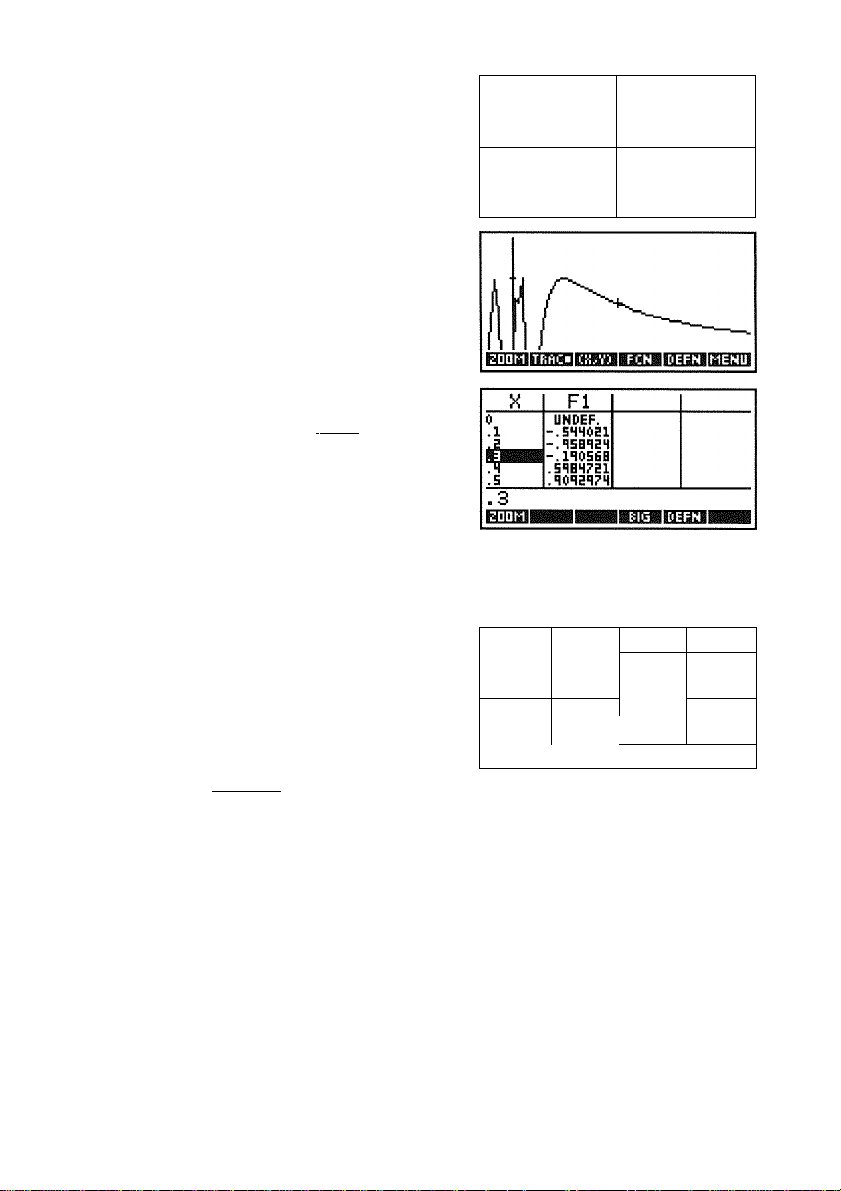
4.
Plot the graph. Press | plot |. The
coordinates show that when .»=0, Kjk)
is undefined.
(If your plot does not look like this,
try resetting the default plot settings;
Press ■ [SETUP-PLOT]
■ [CLEAR].)
Function
Parametric
Polar
Sequence
Solye w
FUNCTION SVM6DÜC
F200 =
v<'FKH)=siHa^K>
F3(X)=
F4<X)=
F5<H)= w
FUNCTION SYMBOLIC SETUP
ANGLE MEASURE:
CHOOSE ANGLE MEASURE
............................
K; 0 FKK
Radian
t
: UNDEFINED IBiann
1-14 Getting Started
Page 23
5. Trace the plot. Move the crosshairs
along the plot by pressing 0] and
B-
............................
/
i ' ' ' ' ' '
....,..
6. Zoom in and zoom out. Press
{{MENU}} {{ZOOM}}, highlight
In 4X4, and press {{OK}}.
To restore the original scale, select
{{ZOOM}} Un-zoom.
7. Display the numbers. To display a
table of data, press |num|. You see
the independent (X) and dependent
(FI) variables listed with sampled
values.
(If your table does not look like this,
try resetting the default numeric
settings : Press ■ [SETUP-NUM]
■ [CLEAR}.)
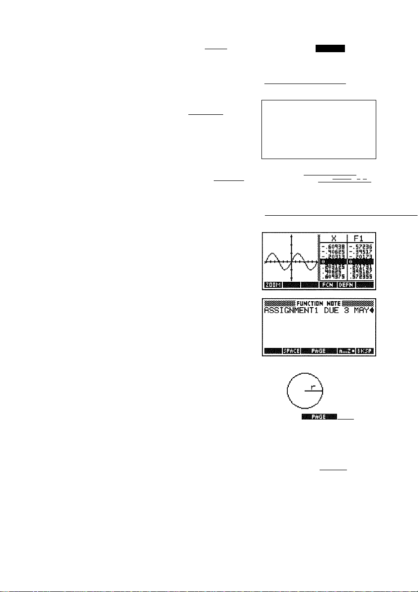
8. Split the screen. Press ■ [VIEWS],
then select Plot-Table {{OK}} to
display these two views
simultaneously.
K:1.3 FKK
i; .sissBas
K FI
-.60H3B -.HH?S3
-.HOSES
-.g03I3
s. HOSES
I.60H3P5
-.SEBBH
.SEBB35
.HH?535
Press I PLOT I to view the full-screen
plot again.
Getting Started 1-15
Page 24
Automatic With this example you have defined a new aplet-an aplet
Saving containing data for the solution of y = sin(l/x). The data are
automatically saved in the Function aplet. If you want to create
another aplet based on Function, then you can give this one a
new name in the Library ({{SAVE}}).
To keep as much memory available for storage as possible,
delete aplets you no longer need.
Annotating The Note view (■ [NOTE}) attaches a note to the current
with Notes aplet. See “Notes and Sketches" later in this chapter.
Annotating The Sketch view (■ [SKETCH]) attaches a picture to the
with Sketches current aplet. See “Notes and Sketches” later in this chapter.
Calculating in You can do calculations in aplets wherever you can enter
Aplets numbers or expressions. Use the math keys on the keyboard
or use operations from the | math | menu list. Chapter 2
discusses math calculations.
Catalogs and Editors
The HP 38G has several catalogs and editors. They access
features and stored values (numbers or text or other items)
that are not part of aplets. A catalog lists items, which you can
delete or transmit. An editor lets you create or modify items
and numbers.
Catalogs/Editors
Cataloe/Editor Contents
Library ((051) Aplets.
List (■ [UST]) Lists. In Home, lists are enclosed in {].
Matrix
One- and two-dimensional arrays. In
(■ [MATRIX]) Home, arrays are enclosed in [ ].
Notepad
(■ [NOTEPAD])
Program
(■ [PROGRAM])
Notes (short text entries).
Programs created by a user.
1-16 Getting Started
Page 25

Storing £uid Recalling Variables
Variables are storage locations for numbers or values. The
HP 38G has different categories of variables for different kinds
of data. The names for the variables are predefined. For real
numbers, there are 27 variable names available, A through Z
and 0. (Other categories and their names are in chapter 2.)
A variable holds just one value, so if you store a new number
in it, any previous number is lost.
To store a
number
To recall a number
You can store a number from Home’s edit line into a named
variable with the {{STO^}} (store) menu key. ({{STO^}}
appears on a menu-key label whenever it is possible to store a
value.) For example.
75{{STO^)} [TZzIA
ENTER
When you press | enter), the number 75 is stored into the
variable named A.
To store the last answer, you don’t need to re-type the
number:
{{STO>}} [aIzIB
enter
This stores 75 (the last result) in B.
In Home, to recall a value from a stored variable back to the
edit line, just type the name of the variable and press | enter].
i A...Z IA [enter! 75
7 5^A4
75
Ans ►Bi
75
Getting Started 1-17
Page 26

“Deleting”
Variables
A variable always has a value in it, even if that value is zero.
When you store another value into a variable, it overwrites the
previous value. So you cannot delete a variable’s value, but
you can overwrite it.
The predefined variable names (such as A through Z) always
exist; you cannot change or delete them.
Home and
Aplet
Variables
Most variables are Home variables, which means they are
shared throughout the different contexts of the calculator.
Some variables are aplet variables, which means they apply
only to the current aplet. Aplet variables are data sets,
expressions, and settings made within an aplet.
Notes and Sketches
The HP 38G has compact text and picture editors for entering
notes and sketches.
® The Notepad is an independent collection of notes.
* Each aplet includes a Note view and a Sketch view for
that aplet only.
Note View and Sketch View
You can attach text to an aplet in its Note view (■ [NOTE]),
or attach pictures to it in its Sketch view (■ [SKETCH]).
To write a note 1. In an aplet, press ■ [NOTE] for the Note view.
In Note view
2. Use the note editing keys shown below.
3. Set Alpha lock (([A...Z}}) for quick entry of letters. For
lowercase Alpha lock, press ■ ((A...Z}}.
® To type a single letter of the opposite case, press
■ letter.
4. Your work is automatically saved. When done, turn off
Alpha lock (by pressing ([A...Zh]}) if you want to go to
Home. (Otherwise, the | home | key will still type A.)
1-18 Getting Started
Page 27

Note Editing
Keys
Key Meaning
{{SPACE}} Space key for text entry.
{{APACE}} Displays previous page of the note.
{{PAGET}}
{{A...Z}}
■ {{A...Z}} Lower-case Alpha-lock.
{{BKSP}}
(HD
1 enter!
H {CLEAR] Erases the entire note.
1 VAR|
1 MATH 1
■ [CHARS] Displays special characters. To type one,
Displays next page of the note.
Alpha-lock for letter entry.
Backspaces cursor and deletes character.
Deletes current character.
Starts a new line.
Menu for entering variable names, and
contents of variables.
Menu for entering math operations,
program commands, and constant names.
highlight it and press {{ECHO}}. Pressing
{{OK}} copies the character and closes the
CHARS screen.
To import a You can import a note from the Notepad into an aplet's Note
note view, and vice-versa.
1. Open the destination note in the Notepad or in the Note
view of an aplet.
2. Press I var|.
* If the source note is in the Notepad, press {{HOME}},
highlight Notepad in the left-hand list, then highlight
the name of the source note in the right-hand list.
* If the source note is part of the current aplet, press
{{APLET}}, highlight Note in the left-hand list, then
press 0 and highlight NoteText in the right-hand
list.
3. Press {{VALUE}} {{OK}} to recall the contents of the source
note into the destination note.
Getting Started 1-19
Page 28

Sketch Keys
To draw a
sketch
Key Meanine
{{STO^}}
{{NEWP}}
{{APACE}}
{{PAGET}}
{{TEXT}}
{{DRAW}}
fPEH
■ [CLEAR]
0
1. In an aplet, press I
2. Press {{DRAW}}.
Stores the specified portion of the
current sketch to a graphics
variable (G1 through GO).
Adds a new, blank page to the
current sketch set.
Displays previous sketch in the
sketch set. Animates if held down.
Displays next sketch in the sketch
set. Animates if held down.
Opens the edit line to type a text
label.
Displays the menu-key labels for
drawing (below).
Deletes the current sketch.
Erases the entire sketch set.
Turns off the menu-key labels. Press
any menu key to restore them.
I
[SKETCH] for the Sketch view.
3. Use the arrow keys to move the crosshairs (graphics
cursor). To draw lines, boxes, or circles, use the menu keys
(described next).
4. When done drawing, press {{OK}}. Your work is
automatically saved. Press any other view key or | home | to
exit the Sketch view.
1-20 Getting Started
Page 29

To draw a line 1. In Sketch view, press {{DRAW}} and move the cursor to
where you want to start the line
2. Press {{LINE}}. This turns on line-drawing.
3. Move the cursor in any direction to the end point for the
line.
4. Press {{OK}} to finish the line.
To draw a box 1. In Sketch view, press {{DRAW}} and move the cursor to
where you want any corner of the box to be.
2. Press {{BOX}}. This turns on box-drawing.
3. Move the cursor to mark the opposite corner for the box.
You can adjust the size of the box by moving the cursor.
4. Press {{OK}} to finish the box.
To draw a 1. In Sketch view, press {{DRAW}} and move the cursor to
circle where you want the center of the circle to be.
2. Press {{CIRCL}}. This turns on circle-drawing.
3. Move the cursor the distance of the radius.
4. Press {{OK}} to draw the circle.
Getting Started 1-21
Page 30

DRAW Keys
Key
Meaning
{{DOT-f}},
{{DOT-}} move.
{{LINE}}
Dot on, dot off. Turns pixels on/off as crosshairs
Draws a line from the cursor’s starting position
to the point at which you press {{ok}}. You can
draw a line at any angle by moving the cursor.
{{BOX}}
Draws a box from the cursor's starting position
to the point at which you press {{OK}}.
{{CIRCL}}
Draws a circle. The cursor’s starting position is
the center of the circle. The cursor’s ending
position (when you press {{ok}}) defines the
radius.
To label parts 1. Press {{TEXT}} and type the text in the edit line. To lock
of a sketch the Alpha shift on, press {{A...Z}} (for uppercase) or
■ {{A...Z}} (for lowercase).
2. To make the label a smaller character size, turn off
{{BIG«}}. (Pressing {{BIG}} turns on {{BIGh}} and vice-
versa.) The smaller character size cannot display
lowercase letters.
3. Press {{OK}}. Use the arrow keys to position the label where
you want it.
4. Press {{OK}} again to affix the label.
5. Press {{DRAW}} to continue drawing, or press | home | to
exit Sketch view.
To create a set You can create a sequence of up to ten sketches. This allows
of sketches for simple animation.
« After making a sketch, press {{NEWP}} to add a new, blank
page that will follow the current page. You can now make
a new sketch. The new image becomes part of the current
set of sketches.
® To view the next sketch in an existing set, press
{{PAGET}}. Hold {{PAGET}} down for animation.
® To remove the current page in the current sketch series,
press [on |.
1-22 Getting Started
Page 31

To store into a You can define a portion of a sketch inside a box, and then
graphics store that graphic into a graphics variable.
variable
1. In the Sketch view, display the sketch you want to copy
(store into a variable).
2. Press {{STO^}}. Highlight the variable name you want to
use and press {{OK}}.
3. Draw a box around the whole screen or around the
portion you want to copy: move the cursor to one corner,
press {{OK}}, then move the cursor to another corner and
press {{OK}}.
To recall a
graphics
variable
The Notepad
1. Open the Sketch view in the destination aplet.
2. Press I VAR I {{HOME}}. Highlight Graphic, then press
and highlight the name of the variable (G1, etc.).
3. Press {{VALUE}} {{OK}} to recall the contents of the
graphics variable.
4. Move the box to where you would like to copy the graphic,
then press {{ok}}.
You can store as many notes as you want in the Notepad
(■ {NOTEPAD}). These notes are independent of any aplet.
The Notepad catalog lists the existing entries by name . It does
not include notes that were created in Note view (■ {NOTE}).
IHDTE CBTftLDGi
TO DO
PHONE NUMBERS
nMUzmii
Getting Started 1-23
Page 32

To write a note 1. In the Notepad, press {{EDIT}} to modify the highlighted
in the Notepad note or press {{new}} to start a new note. For a new note,
type in a name and press {{OK}}.
2. This opens the note for you to write and edit. Use the Note
editing keys as in Note view (see page 1-19).
3. When you are done, you can leave the Notepad by
pressing I HOME I or an aplet view key. Your work is
automatically saved.
Notepad
Catalog Keys
Key
{{EDIT}}
{{NEW}}
{{SEND}}
{{RECV}} (receive)
K [CLEAR]
Meaning
Opens the selected note for editing.
Opens a new note, and asks for a
name.
Transmits the selected note to
another HP 38G or a disk drive. See
also page 1-27.
Receives a note being transmitted
from another HP 38G or a disk
drive. See also page 1-27.
Deletes the selected note.
Deletes all notes in the catalog.
1-24 Getting Started
Page 33

Managing Aplets
Once you have entered information into an aplet, you have
defined a new version of an aplet. The information is
automatically saved under the current aplet name, such as
“Function.” To create additional aplets of the same type, you
must give the current aplet a new name.
The Library is where you go to manage your aplets. Press
jiiBl. Highlight (using the arrow keys) the name of the aplet
you want to act on.
currentaplet
names of
aplets
The current aplet is highlighted.
tftPLET UERflRV
Function
Parametric
Polar
Sequence
Solue f
library Keys
To open an
aplet
Key Meanine
{{SAVE}}
{{RESET}} Resets the default values and
{{SORT}}
{{SEND}}
{{RECV}} (receive)
{{START}} (or 1 enter))
Press (LIB 1 to open the Library. Highlight the aplet and
press {{START}} or I ENTER]. The aplet’s main view appears.
Instead of pressing {{START}}, you can press a view key
(like I PLOT I, |symb|, or |num|) to immediately display that
view of the aplet.
Saves the highlighted apiet with a
name.
settings in the highlighted aplet.
Rearranges the aplet list.
Transmits the highlighted aplet to
another HP 38G or a storage device.
Receives the aplet being sent from
another HP 38G or storage device.
Opens the highlighted aplet.
Getting Started 1-25
Page 34

To name an
aplet
1. Press I LIB I to open the Library. Highlight the aplet to name.
2. Press {{SAVE}} and enter a name. Press {{OK}} to confirm
it, {{CANCL}} to cancel it.
To create a
new aplet
To delete an
aplet
To clear an
aplet
To sort the
aplet list
You can create a new aplet based on an existing aplet.
1. Open the aplet you want to start from.
2. Enter or modify its information (equations, data, settings).
This defines a new version of the aplet. All information is
saved until you clear it or edit it.
3. To name the aplet for future access, use {{SAVE}} in the
Library.
Open the Library, highlight the custom (not built-in) aplet to
delete, and press |del|. To delete all custom aplets, press
■ {CLEAR}.
You cannot delete the built-in aplets. You can clear their data
and reset default settings using {{reset}}.
Resetting an aplet clears all data and resets all default settings.
® To reset an aplet, open the Library, select the aplet and
press {{RESET}}.
In the Library, press {{SORT}}. Select the sorting scheme and
press I ENTER I.
e Chronologically produces a chronological order by
most recent use of the aplets. (The last-used aplet appears
first, and so on.)
® Alphabetically produces an alphabetical order by
aplet name.
1-26 Getting Started
Page 35

Sending and Receiving Aplets
A convenient way to distribute or share problems in class and
to turn in homework is to transmit (copy) aplets directly from
one HP 38G to another. This takes place via the infrared port.
You can also send (copy) and receive aplets to/from a remote
storage device (aplet disk drive or computer). This takes
place via a cable connection and requires an aplet disk drive
or specialized software running on a PC or Mac (such as a
connectivity kit).
To transmit an 1. Connect the storage device to the calculator by cable
aplet or
align the two calculators' infrared ports by matching up
the triangle marks on the rims of the calculators. Place the
calculators no more than 2 inches (5 cm) apart.
2. Sending calculator: Open the Library, highlight the aplet
to send, and press {{send}}.
e You have two options : another HP 38G or a disk drive
(or a computer). Highlight your selection and press
{{OK}}.
e If transmitting to a disk drive (aplet disk drive or
computer), you have the options of sending to the
current (default) directory or to another directory.
Getting Started 1-27
Page 36

3. Receiving calculator : Open the Library and press
{{RECV}}.
* You have two options : another HP 38G or a disk drive
(or computer). Highlight your selection and press
{{OK}}.
If receiving from a remote storage device (aplet disk drive or
computer), you will see a list of aplets in its current directory.
You can choose a different directory to copy from. Check as
many items as you would like to receive.
1-28 Getting Started
Page 37

Mathematical Calculations
The most commonly used math operations are on the
keyboard. Access to the rest of the math functions is via the
MATH menu (press |math|).
The MATH menu also contains commands to use for
programming.
How to Do Calculations
Where to Start The home base for the calculator is Home (press |home |).
You can do all calculations here, and you can access all
[ MATH I operations.
Entering Expressions
Enter an expression into the HP 38G in the same left-toright order that you would write the expression.This is
called algebraic entry.
To enter functions, select the key or MATH menu item for
that function. You can also use Alpha keys to spell out a
function's name.
Example
e Press I ENTER I to evaluate the expression you have in the
edit line (where the blinking cursor is). An expression can
contain numbers, functions, and variables.
Calculate 23^-(14Vs)-!-(-3)ln45 with these keystrokes.
23 ■ [x^] □Ш14 0Ш
8ШШЕ1]30И[Ш] 45
m riiJiTFI 23a-14*T8/'-3*LNC45)
Ш LtNitKJ 579.245381391
Mathematical Calculations 2-1
Page 38

Long Results
If the result is too long to fit in the display line, press 0 to
highlight it and then press {{SHOW}}.
Negative
Numbers
Scientific
Notation
powers of 10)
Type [^to start a negative number or to insert a negative
sign.
If a negative number will be raised to a power, enclose it in
parentheses. For example, (—5)^= 25, whereas - 5^= - 25.
A number like 5x10"' or 3.21x10"' is written in scientific
notation, that is, in terms of powers of ten. This is simpler to
work with than 50000 or 0.000000321. To enter numbers like
these, use [EEX]. (This is easier than using fillOfx^.)
Example
Calculate ------------------------
4TEEXini3F]6
■ [EEX] 2 0 3® [EEX]
(4xl0"')(6xl0')
as shown :
3x10
4E-3*6E2x3E-5
FF|5 I ENTER I
Explicit and You should include the times sign where you expect
Implicit multiplication in an expression. It is clearest to enter AS as
Multiplication and A(B+C] as A* (B+c).
80000
Implied multiplication takes place when two operands appear
with no operator in between. If you enter AB, for example, the
result is A* B.
Parentheses Parentheses are necessary to enclose arguments for
functions, such as SIN (4 5). You can omit the final
parenthesis at the end of an edit line.
Parentheses are also important in specifying the order of
operation. Mf/toui parentheses, the HP 38G calculates
according to the order of algebraic precedence (the next
topic). Following are some examples using parentheses.
2-2 Mathematical Calculations
Page 39

Examples
Algebraic
Precedence
(Order of
Evaluation)
Enterine...
[Ml 45 0 ■ [it]
[Ml 45 eg 0 H [it]
1 Vx 1 85 01 9
[W1 B 55 0 9 Q]
Functions within an expression are evaluated in the following
order of precedence. Functions with the same precedence
are evaluated in order from left to right.
1.
Expressions within parentheses. Nested parentheses are
evaluated from inner to outer.
Prefix functions, such as SIN and LOG.
Postfix functions, such as !
Power function,NTHROOT.
Negation, multiplication, and division.
6. Addition and subtraction.
7. AND and NOT.
8.
OR and XOR.
9. Left argument of | (where).
10. Equals, =.
Calculates...
sin (45 -r tt)
sin (45) + -IT
yfExQ
VS5x9
Fractions The HP 38G can display fractions of the form alb. To set
Fractions mode, select Fractions as the Number Format in
Home Modes (■ [MODES]). Specify the number of decimal
places to use for the denominator. For instance, in Fraction 2
format, 29/1000 becomes 2/69 .
To enter a fraction use the [7] key.
Largest and
Smallest
Numbers
The smallest number the HP 38G can represent is 1 xlO“®®
(1E-499). A smaller result is displayed as zero. The largest
number is 9.99999999999x10®’. A larger result is still
displayed as this number.
Mathematical Calculations 2-3
Page 40

Complex Numbers
Complex The HP 38G can return a complex number as a result for
Results some math functions, A complex number appears as an
ordered pair (x, y), where x is the real part and y is the
imaginary part. For example, entering returns (0,1).
To enter Enter the number in either of these forms, where x is the real
complex part, y is the imaginary part, and i is the imaginary constant,
numbers ,JZ\-
e (X, y) or
e X + iy ,
To type i, press ■ | A...Z 11, or copy i from the Constant
category in the MATH menu.
Clearing Numbers
• I DEL I clears the character under the cursor (|). j
backspaces when the cursor is after the last character.
® CANCEL (|ON|) clears the edit line.
• ■ [CLEAR] clears all input and output in the display,
including the display history.
Using Previous Results
The Home display shows you four lines of input/output
history. An unlimited (except by memory) number of
previous lines are available by scrolling. You can retrieve and
reuse any of these values or expressions.
Last Answer You can reuse the last answer at any point in the edit line by
([ANSWER]) pressing ■ [ANSWER], This recalls the variable Ans (last
answer), the result from your last | enter].
The variable Ans is different from the numbers in Home's
display history, A value in Ans is stored internally with the full
precision of the calculated result, whereas the displayed
numbers match the display mode. When you retrieve a
number from Ans, you obtain the result to its full precision.
When you retrieve a number from Home’s display history, you
obtain exactly what was displayed.
2-4 Mathematical Calculations
Page 41

Note that pressing | enter] enters (or re-enters) the last input,
whereas pressing ■ [ANSWER] copies the last result into the
edit line.
Continuing a You can continue calculating with your last result, Ans,
Calculation simply by pressing an operator key.
50 [7] 3 I ENTER I
[+] 25 I ENTER I
50-^3
flns+25
^HDME
16.6666666667
41.6666666667
Accessing
the Display
History
Pressing 1 ENTER 1 again
updates the value of Ans and
repeats the operation.
Pressing Q turns on the highlight bar in the display history.
Key Meaning
S.E
{{COPY}} Copies the highlighted expression
{{SHOW}} Displays the current expression in
mD
■ {CLEAR}
flns-E25
Scroll through the display history
and highlight display lines.
to the position of the cursor in the
edit line.
standard mathematical form.
Deletes the highlighted expression
from the display history, unless
there is a cursor in the edit line.
Clears all lines of display history
and the edit line.
»HDHE
16.6666666667
41.6666666667
66.6666666667
Mathematical Calculations 2-5
Page 42

Clearing the
Display
History
It's a good habit to clear the display history (■ [CLEAR])
whenever you are done working in Home.
It saves calculator memory to clear the display history.
Remember that all your previous inputs and results are saved
until you clear them.
Clearing the
Edit Line
* [ DEL I deletes single characters in the edit line.
(CANCEL) clears the entire edit line.
Storing in Variables
You can store numbers or expressions from any previous
input or result into variables.
Numeric
Precision
To store a value
A number stored in a variable is always stored as a 12-digit
mantissa with a 3-digit exponent. Numeric precision in the
display, however, depends on the display mode (Standard,
Fbced, Scientific, Engineering, or Fraction). A displayed
number has only the precision that is displayed.
Press {{STO>}} I letter I ENTER I, where letter represents the
one-letter variable name for real numbers.
6 {{STO^}} [aIz] B
ENTER
You can store the last answer the same way:
13 Q 5 I ENTER I
{{STO^}} A fENTE^
BHai
la-'S
Hnsfrfl
mil
2.6
2.6
To store any
previous value
To recall a
value
If the value you want to store is somewhere else in the Home
history, first copy it to the edit line: highlight the line (using
arrow keys) and press {{COPY}}. Then store it.
Type the name of the variable and press | enter].
|A...Z|A I ENTER I 2.6
2-6 Mathematical Calculations
Page 43

The VAR Menu
Another way to retrieve a variable is to use the VAR
(variables) menu. The VAR menu contains the Home
variables, as well as the aplet variables for the current aplet.
The VAR menu is organized by category. For each category of
variables on the left, there is a list of variables on the right.
The highlighted category is the current category.
current
category
The {{HOME}} and {{APLET}} menu keys switch to Home and
Aplet variables. The h symbol indicates what is "on": {{HOM*}}
means that the Home variables are displayed.
«niTOWWWtWOWW« I
iComplex ■
Graphic
Library Z3
List ¥ Z4 T
Z1
Z2
variable
names
Home
Variables
The Home variables are the ones you most commonly use
while doing calculations in Home. Any value (or other data)
you store must be stored in a variable of the correct type.
Cateeorv
Complex Z1 through Z9 and ZO.
Graphic G1 through G9 and GO.
Library
List LI through L9 and ID.
Matrix Ml through M9 and MO.
Modes
Notepad User-provided.
Program User-provided.
Real A through Z and 6.
Available Names
aplets
The MODES screen (■ {MODES})
stores values in these variables.
Mathematical Calculations 2-7
Page 44

Home variables retain their values regardless of context:
Home, the aplets, and the editors recognize the Home
variables and retain whatever was last stored in them. This
sharing allows you to work on the same problem in different
places (such as Home and the Function aplet) without having
to update a variable whenever it is recalculated.
If you have not stored anything in a real variable, then it
contains the value zero. (It is never “empty.”)
To access a 1. Press | var | to display the VAR menu. Set {{HOMa}}, if
Home variable necessary by pressing {{HOME}}.
2. Use 0 and 0 to scroll through the alphabetical list of
categories. To skip directly to a starting letter, press a letter
key. To switch between the category list (left) and the
variable list (right), use 0 and 0.
3. Highlight the name of the variable you want.
• To copy the name of the variable into the edit line,
press {{OK}}. (NAME is set: the menu label shows
{{NAM«}}).
To copy the value of the variable into the edit line, set VALUE
(press {{VALUE}} to make it {{VALU«}}) and press {{OK}}.
2-8 Mathematical Calculations
Page 45

Aplet The variable types in the table below are aplet variables that
Variables you use to define aplet functions and to store some kinds of
aplet data. They are usually found in the Symbolic view or the
Numeric view of an aplet.
Aolet Cateeorv
Function
Parametric XI, Y1 through X9, Y9 and XO,
Polar R1 through R9 and RO
Sequence U1 through U9 and UO
Solve El through E9 and EO
Statistical data Cl through C9 and CO
As you load new aplets in the HP 38G, their names and
variables will be added to the VAR menu.
In addition, there are other aplet variables that are record
settings, such as those in the Setup views. These types of
variables (like NumStart and Xtick) are listed in chapter 8,
Programming, since you do not need to know their names
except when programming.
Available Names
FI through P9 and FO
(Symbolic view)
YO (Symbolic view)
(Symbolic view)
(Symbolic view)
(Symbolic view)
(Numeric view)
Mathematical Calculations 2-9
Page 46

To access an The {{APLET}} menu key in the VAR menu switches the menu
aplet variable ¡¡st to aplet variables. The ■ symbol indicates what is "on":
{{APLEb}} means that aplet variables are displayed.
1. Open the aplet whose variable you want to recall.
2. Press I VAR I to display the VAR menu. Set {{apleb}}, if
necessary by pressing {{aplet}}.
I^^FUNCTIBN
Plot ■ fixes
Plot FCN
Symbolic
Numeric v
Connect
Coord
FastRes v
3. Highlight the view on the left side. If you’je not sure which
view it’s in, just scroll through the view names and check
the names of the variables on the right.
4. Press {{OK}} or to switch to the list of variable names
on the right side.
5. Highlight the name of the variable you want. To copy its
name, turn on {{NAM»}}. To retrieve its value, turn on
{{valub}}. Press {{OK}}.
You can do this in Home if the aplet you want is current; that
is, it was the last one open.
Symbolic Calculations
Formal Names
Note
A formal name acts as a placeholder—it does not represent a
value, just a symbol. In Home or in a program, the expression
(s 1 * s 2) ^ always returns the expression (s 1 * s 2) ^. The
real variables in {A*B) ^ on the pther hand, are evaluated to
a number, the value of which depends on what is currently
stored in A and B.
Remember that there is always a value in a real variable,
even if it is zero.
2-10 Mathematical Calculations
Page 47

You can mix formal names and real variables. Evaluating
(A*s2) ^ will substitute a number for A but not for s2.
If you want to evaluate an expression like (sl*s2) ^
numerically, you can do so using the I (where} command,
listed in the MATH menu under the Symbolic category. For
instance, if you wanted si = 3 and s2 = 4, you would enter
(sl*s2) ''2 I (sl=3, s2=4). (The = symbol is in the CHARS
menu: press ■ [CHARS] {{OK}}).
Indeflnite
Integrals
Definite
Integrals
Derivatives
To find the indefinite integral (with a symbolic rather than
numeric result), use formal variables (that is, sO through s5)
for a limit of integration. For instance, to compute
I (6x - 5)dx ,
ehter the integration as / (0, si, 6*x'-5, X).
0 and si are the lower and upper limits, and X is the variable
of integration.
1. Enter the the integration expression in the Home edit line.
(The f symbol in the the CHARS menu.)
2. Press [ENTER], which produces an intermediate result.
3. Press 0 ([COPY]} [ENTER] to complete the evaluation.
The result of /(0,sl,6*X2-5,X) should be
-(5*sl)+6*(s 1^3/3), that is, 2x3-5x.Translators: in Comma
mode; change syntax to use periods.
To find the definite integral (with a numeric result), use
numeric values (numbers or real variables containing
numbers) for both the upper and lower limits. For instance, if
you enter J(-2,3,6*X2-5,X)and press [ENTER] , the result is
45.
To find the symbolic derivative of an expression, use a formal
variable (s 1, etc.) to define the derivative. For example, to
find D/6x*-5x), enter 3sl (6*sl^- 5*sl) .The result is
6*(2*sl) -5, which is equal to 12x—5.
If you use real variables or numbers in the derivative, the
calculator will find a numeric result.
Mathematical Calculations 2-11
Page 48

Composition of You can define a function of another function using the
Functions Function aplet (|lib| Function). That is, f(g(xy) can be
entered into the Symbolic view of Function as
F1(X) -expression!
F2 (X) = expression2
F3 (X) = FI {F2 (X) )
Using Math Functions
Selecting To enter a function, type it in or select its name from the
Functions MATH menu.
The MATH Menu
The MATH menu provides access to Math Functions,
Programming Commands, and Programming Constants.
The MATH menu is organized by category. For each category
of functions on the left, there is a list of function names on the
right. The highlighted category is the current category.
current
category
Re.3l C
Stat-Two
Symbolic FLOOR
Tests ▼
»8»iopniTMMu;iai
• When you press | math |, you see the menu list of Math
Functions. The menu key {{MTHa}} indicates that the Math
Functions list is "on."
« To display the menu list of Program Commands, press
{{CMOS}}. To display the menu list of Program Constants,
press {{CONS}}. To re-display the Math Functions, press
{{MTH}}.
The programming commands and programming constants
are discussed in chapter 8, Programming.
FUNCTIDNS^»|
CEILING
DEG-^RflD -J
FNROOT T
•
IB3MIHII3Ì
functions
2-12 Mathematical Calculations
Page 49

To copy a 1. Press | math | to display the MATH menu. The categories
function appear in alphabetical order. Use 0 and 0 to scroll
through the categories. To skip directly to a starting letter,
press a letter key.
2. The list of functions (on the right) applies to the currently
highlighted category (on the left). Use 0 and 0 to
switch between the category list and the function list.
3. Highlight the name of the function you want and press
{{OK}}. This copies the function name (and an initial
parenthesis, if appropriate) to the edit line.
Function
Categories
Calculus
Complex
numbers
Constant
Hyperbolic trig
Lists
Loop
Matrices
Polynomial
Probability
Real numbers
Statistics-Two
Variable
Symbolic
Tests
Trigonometry
The Math Functions by Category
Following are definitions for all categories of functions except
List, Matrbc, and Statistics, each of which appears in its own
chapter. Except for the keyboard operations, which do not
appear in the MATH menu, all other functions are listed by
their category in the MATH menu.
Syntax Each function’s definition includes its syntax, that is, the exact
order and spelling of a function’s name, its delimiters
(punctuation), and its arguments. Note that the syntax does
not include spaces.
Mathematical Calculations 2-13
Page 50

Keyboard
Functions
The most frequently used functions appear on the keyboard.
The keyboard functions are the only math functions that do
not appear in the MATH menu. Many of the keyboard
functions also accept complex numbers as arguments.
0.Q.0.0
Add, Subtract, Multiply, Divide. Also accept complex numbers.
value 1+ value2, etc.
m i e l
Natural exponential. Also accepts complex numbers.
e''value
■ [LN]
Natural logarithm. Also accepts complex numbers.
IM [value]
■ [101
Exponential (antilogarithm). Also accepts complex numbers.
10''value
■ [LOG]
Common logarithm. Also accepts complex numbers.
LOG [value]
|SIN|, |COS|,
|TAN|
Sine, cosine, tangent. Inputs and outputs depend on the current
angle format (Degrees, Radians, or Grads).
SIN(oo/ue)
COS [value]
TAN [value]
■ [ASIN] Arc sine : sin^'x Output ranges from -90° to 90°, -'ir/2 to tt/2,
or -100 to 100 grads. Inputs and outputs depend on the current
angle format.Also accepts complex numbers.
■ [ACOS]
ASIN(UO/ue)
Arc cosine: cos^'x. Output ranges from 0° to 180°, 0 to tt, or 0 to
200 grads. Inputs and outputs depend on the current angle
format. Also accepts complex numbers.
ACOS [value]
2-14 Mathematical Calculations
Page 51

[ATAN]
Arc tangent: tan^'x. Output ranges from -90° to 90°, -Tr/2 to
77/2, or -100 to 100 grads. Inputs and outputs depend on the
current angle format. Also accepts complex numbers.
AT AN (oa/ue)
l[J^]
Square. Also accepts complex numbers.
value‘
Square root. Also accepts complex numbers.
V~value
[^]
K’]
Pi, a constant.
Multiplicative inverse (reciprocal). For a complex number, the
reciprocal is
X +y X +y
value''-!
EU
Negation. Also accepts complex numbers.
-value
IZ]
Power (x raised toy). Also accepts complex numbers.
value'‘power
! [ABS] Absolute value. For a complex number, this is •/
ABS [value)
ABS( (x,y) )
2 2
X +y .
I Takes the nth root of x.
roo/NTHROOTna/ue
Example: 3 B S/x 8 returns 2.
Mathematical Calculations 2-15
Page 52

Calculus
Functions
You will find the symbols for the calculus functions derivative
and integral in the CHARS menu (■ [CHARS]) as well as the
MATH menu.
a
f
TAYLOR
Differentiates expression with respect to the variable of
differentiation. Use a formal variable (si, etc.) for a non
numeric result.
doariable(expression)
Example: asl (sl^+3*sl) returns 2*sl+3
Integrates expression from lower to upper limits with respect to
the variable of integration. To find the definite (numeric)
integral, both limits must have numeric values (that is, be
numbers or real variables). To find the indefinite integral, one
of the limits must be a formal variable (si, etc.).
/ {lower, upper, expression, variable')
Example; /( 0, si, 2*X+3 , X) |ENTER| |T| ffCOPY}} |enter]
finds the indefinite result 3*sl+2*(sl''2/2)
Calculates the nth order Taylor’s polynomial of expression at the
point where the given variable =0.
TAYLOR {expresslon,variable,n)
2-16 Mathematical Calculations
Page 53

Complex-
Number
Functions
These functions are for complex numbers only. You can also
use complex numbers with all trigonometric and hyperbolic
functions, and with some real-number and keyboard
functions. Enter complex numbers in the form (x,y), where x
is the real part and y is the imaginary part.
ARC
CONJ
IM
RE
Argument. Finds the angle defined by a complex number.
Inputs and outputs use the current angle format in Modes.
ARG{ ir,0) )
Complex conjugate. Conjugation is the negation (sign reversal)
of the imaginary part of a complex number.
CONJ( lx,y) }
Imaginary part, y, of a complex number, (x,y).
IM ((x,y))
Real part x, of a complex number, (x,y).
RE ((X,y))
Mathematical Calculations 2-17
Page 54

Constants
The HP 38G has an internal numeric representation for these
constants.
e
!
MAXREAL
MINREAL
n
Natural logarithm base. Internally represented as
2.71828182846.
Imaginary value for , the complex number (0,1).
Maximum real number. Internally represented as
9.99999999999X10“.
MAXREAL
Minimum real number. Internally represented as 1 x 10 “
MINREAL
The ratio perimeter: diameter. Internally represented as
3.14159265359.
TT
2-18 Mathematical Calculations
Page 55

Hyperbolic
Trigonometry
The hyperbolic trigonometry functions can also take complex
numbers as arguments.
ACOSH
Inverse hyperbolic cosine: cosh'r.
ACOsm value)
ALOG
Antilogarithm (exponential). This is more accurate than 10''x
due to limitations of the power function.
ALOG [value]
ASINH
ATANH
COSH
Inverse hyperbolic sine : sinh''x.
ASINH (ua/ue)
Inverse hyperbolic tangent: tanh~'x. If the input is ± 1, an
Infinite Result occurs.
ATANH (ufl/ue)
Hyperbolic cosine: (e'4€^')/2.
COSH (value)
SINH
TANH
EXP Natural exponential. This is more accurate than e''x due to
Hyperbolic sine.
SlNH(oa/«e)
Hyperbolic tangent.
TANH(wa/iie)
limitations of the power function.
EXP (value)
EXPMl
LNPl Natural log plus 1 : ln(x+l). This is more accurate than LN
Exponent minus 1 : e'-1. This is more accurate than EXP when
X is close to zero.
EXPMl (value)
when X is close to zero.
LNPl (value)
Mathematical Calculations 2-19
Page 56

List Functions These functions are for list data stored in list variables. See
chapter 7, Using Lists.
Loop Functions The loop functions display a result after evaluating an
expression a given number of times.
ITERATE Repeatedly (the specified dimes') evaluates an expression in
terms of variable. The value for variable is updated each time,
starting with initialvalue.
ITERATE {expression, variable, initialvalue, ^imes)
RECURSE Provides a method of defining a sequence without using the
Symbolic view of the Sequence aplet.
RECURSE {sequencename, term-n, terml, term2)
Example: RECURSE (U,u (N-1) *N, 1,2) {{ST0^}}U1 (N)
This produces the factorial
ui(1)=1
Ul(2)=2
U1(N)=U1(N-1)*N
2 Summation. Finds the sum of expression with respect to variable
from initialvalue to finalvalue.
2 (variable=initialvalue, finalvalue, expression)
Example:2(C=l, 5,C^) returns55.
Matrix These functions are for matrix data stored in matrix variables.
Functions See chapter 8, Using Matrices.
2-20 Mathematical Calculations
Page 57

Polynomial
Functions
Polynomials are products of constants (coefficients) and
variables raised to powers (terms).
POLYCOEF Polynomial coefficients. Returns the coefficients for the
polynomial with the specified roots.
POLYCOEF! [roofs] )
Example: to find the polynomial with roots 2,-3, 4, -5:
POLYCOEF ( [2,-3,4,-5]) returns [1,2 ,-25,-26,120],
representing x%2з¿-25)¿-2%x+\ 20.
POLYEVAL Polynomial evaluation. Evaluates a polynomial with the
specified coefficients for the value of x.
POLYEVAL! [coefficients] , value)
Example: for 25x^—26jc-rl20:
POLYEVAL! [1,2, -25, -25,120] , 8) returns 3432.
POLYFORM Polynomial form. Creates a polynomial in variable] from
expression. Can express the coefficients as a polynomial in
variable2. (The coefficients of the coefficients can be expressed
as polynomials in variables, etc.)
POLYFORM! expression, variable 1,.. .,variable-n)
Example: polyform! !x+1) ''2 + 1,x) returnsX''2+2*x+2 .
POLYROOT
Polynomial roots. Returns the roots for the nth-order polynomial
with the specified n+l coefficients.
polyroot! [coefficients])
Example: forx“-i-2x*-25x^-26x+120:
POLYROOT! [1,2,-25,-26,120] ) returns [2,-3,4,-5].
Mathematical Calculations 2-21
Page 58

Probability
Functions
Probability functions are often used in statistical analyses.
COMB
!
PERM
RANDOM
UTPC
UTPF
Number of combinations (without regard to order) of n things
taken rat a time, n!/(r!(n-r)).
COMB (n,r)
Factorial of a positive integer. For non-integers, ! = F(x + 1).
value !
Number of permutations (with regard to order) of n things
taken rat a time, n\/ (_n-r)\.
PERM(n,r)
Random number (between zero and 1). Produced by a pseudo
random number sequence. Becomes the seed for the next
random number.You can set the seed using the command
RANDSEED.
RANDOM
Upper-Tail Chi-Squared Probability given degrees of freedom,
evaluated at value. Returns the probablility that a random
variable is greater than value.
UTPC ( degrees, value )
Upper-Tail Snedecor’s F Probability given numerator degrees of
freedom and denominator degrees of freedom (of the F
distribution), evaluated at value. Returns the probability that a
Snedecor's F random variable is greater than value.
UTPF {numerator, denominator, value)
UTPN
Upper-Tail Normal Probability given mean and variance,
evaluated at value. Returns the probability that a normal
random variable is greater than value for a normal distribution.
(The variance is the square of the standard deviation.)
UTPN ( mean, variance, value )
UTPT Upper-Tail Student's t Probability given degrees of freedom,
evaluated at value. Returns the probability that the Student's t
random variable is greater than value.
UTPT ( degrees, value )
2-22 Mathematical Calculations
Page 59

Real-Number
Functions
Some real-number functions can also take complex
arguments.
CEIUNG
Smallest integer greater than, equal to value.
CEILING (oa/ue)
DEG->RAD Degrees to radians. Converts value from Degrees angle format
to Radians angle format.
DEG—>RA.D (VOltlB)
FLOOR
FNROOT
Greatest integer less than or equal to value.
FLOOR (value)
Function root-finder (like Solver aplet). Finds the value for the
given variable at which expression most nearly evaluates to
zero. Uses guess as initial estimate.
FNROOT (express/ou, variable, guess)
FRAG Fractional part.
FRAC (value)
HMS->
-^HMS
Hours-minutes-seconds to decimal. Converts a number or
expression in H.MMSSs format (time or angle that can include
fractions of a second) to x.x format (number of hours or
degrees with a decimal fraction).
HMS-> ( H.MMSSs)
Decimal to hours-minutes-seconds. Converts a number or
expression in x.x format (number of hours or degrees with a
decimal fraction) to H.MMSSs format (time or angle up to
fractions of a second).
—>HMS (x.x)
INT
MANX
Integer part.
INT (value)
Mantissa (significant digits) of value.
MANT (value)
Mathematical Calculations 2-23
Page 60

MAX
Real-Number Functions, continued
Maximum. The greater of two values.
MAX (value!, value2)
MIN
MOD
%CHANGE
%TOTAL
RAD^DEG
ROUND
SIGN
Minimum. The lesser of two values.
MIN (value!, value2)
Modulo. The remainder of valueHualue2.
value! MOD value2
X percent of y; that is, Ay/100.
%(x,y)
Percent change from x toy, that is, 100(y-x)/x.
%CHANGE(X,y)
Percent total: (100)y/x What percentage of x isy.
%TOTAL(X,y)
Radians to degrees. Converts value from one angle format to
another.
RAD-ADEG (value)
Rounds value to decimal places. Accepts complex numbers.
ROUND {value,places)
Sign of value. If positive, the result is +1. If negative, -1. If zero,
result is zero. For a complex number, this is the unit vector in
the direction of the number
( ^
2 2 ’ I 2 T
X +y yx +y
i
.Y V
TRUNCATE
XPON
SIGN(ua/ue)
SIGN( (x,y) )
Truncates value to decimal p/aces. Accepts complex numbers.
TRUNCATE (value, places)
Exponent of value.
XPON {value)
2-24 Mathematical Calculations
Page 61

Statistics-Two
Symbolic
Functions
These are functions for use with two-variable statistics. See
chapter 5, Statistics.
The symbolic functions are used for symbolic manipulations
of expressions. The variables can be formal or numeric, but
the result is usually in symbolic form (not a number). You will
find the symbols for the symbolic functions = and 1 (where) in
the CHARS menu (|P [CHARS]) as well as the MATH menu.
= (equals')
ISOLATE
UNEAR?
QUAD
QUOTE
Sets an equality for an equation. This is not a logical operator.
(See the Test category.)
expression 1 =expression2
Isolates the first occurrence of variable in expression and
returns an equation, variable=value. The result is a general
solution that represents multiple solutions by including the
(formal) variables s7 to represent any sign and nl to represent
any integer.
ISOLATE {expression, variable)
Tests whether expression is linear for the specified variable.
Returns 0 (false) or 1 (true).
LINEAR? [expression, variable)
Solves quadratic expression for variable and returns an
equation, variable=newexpression. The result is a general
solution that represents both positive and negative solutions by
including the (formal) variable si to represent any sign, -r or - .
QUAD {expression, variable)
Encloses an expression that should not be evaluated
numerically.
QUOTE (expression)
1 (where)
Evaluates expression where each given variable is set to the
given value. Allows numeric evaluation of a symbolic
expression.
expression \ (variable 1 =value 1,variable2=value2,...)
Mathematical Calculations 2-25
Page 62

Test Functions The test functions are logical operators that always return
either a 1 (true') or a 0 (false).
<■ Less than. Returns 1 if true, 0 if false.
value Kaalue2
^ Less than or equal to. Returns 1 if true, 0 if false.
value l^value2
— — Equals (logical test). Returns 1 if true, 0 if false.
value 1 = =value2
Not equal to. Returns 1 if true, 0 if false. i=
value! i=value2
> Greater than. Returns 1 if true, 0 if false.
value I>value2
> Greater than or equal to. Returns 1 if true, 0 if false.
value! ^value2
AND
IFTE
NOT
OR
XOR
Compcires value! and value2. Returns 1 if they cire both non
zero, otherwise returns 0.
value! AND value2
If expression is true, do the trueclause; if not, do the falseclause.
IFTE (expression, trueclause, falseclause)
Example: IFTE(X>0,x^x’)
Returns 1 if value is zero, otherwise returns 0.
NOT value
Returns 1 if either value! or value2 is non-zero, otherwise
returns 0.
value! OR value2
Exclusive OR. Returns 1 if either value! or value2 —but not both
of them—is non-zero, otherwise returns 0.
value! XOR value2
2-26 Mathematical Calculations
Page 63

Trigonometry
Functions
The trigonometry functions can also take complex numbers
as arguments. For SIN, COS, TAN, ASIN, ACOS, and ATAN, see
the Keyboard category (all these functions have keys).
ACOT
ACSC
ASEC
COT
CSC
SEC
Arc cotangent.
ACOT (value)
Arc cosecant.
ACSC {value)
Arc secant.
ASEC {value)
Cotangent: cosx/sinx.
COT {value)
Cosecant: 1/sinx
CSC {value)
Secant: 1/cosx.
SEC {value)
Mathematical Calculations 2-27
Page 64

Page 65

Plotting and Exploring Functions
Types of Plots Graphing is at the heart of the HP 38G. All of the built-in aplets
do graphing. This chapter considers the four main built-in
aplets:
« Function,
® Parametric,
e Polar, and
9 Sequence,
The Solve aplet and Statistics aplet, which also include
graphing, are covered in separate chapters.
Defining a Problem
You start with an aplet and a mathematical function to
explore, like y = mx + h.
General Steps 1. From the Library (| lib |), open the aplet you want. This
determines the type of function you can enter and plot.
2. In the Symbolic view CIsymbQ, enter or select an
expression. Check the angle units in the Symbolic Setup
(■ [SETUP-SYMB]).
3. In the Plot view (|plot1), display the graph. There are
menu keys to explore by tracing and zooming. Optional:
Specify graph settings in the Plot Setup (■ [SETUP-
PLOT]).
4. Explore a table of numeric values in the Numeric view
(I NUM|). Optional: specify table settings in the Numeric
Setup (■ [SETUP-NUM]).
5. All information is automatically stored until you change it.
To preserve the complete aplet as you have set it up, use
the Library to name and save the aplet (chapter 1).
Plotting and Exploring Functions 3-1
Page 66

Select an Aplet
Select the aplet appropriate to your problem : Open the
Library (|lib|), highlight the name of an aplet, and press
{{START}} (or IENTErQ.
® Function . This aplet can define rectangular equations of
the form y = f(x) .
• Parametric . This aplet can define parametric expressions,
which define equations over time, t. They take the forms
jf = /'(0andy = g(0-
® Polar, This aplet can define polar expressions, which
graph equations in terms of an angle 0.
• Sequence. This aplet can define sequence functions,
which are defined in terms of n or in terms of the previous
terms in the sequence. Sequence plotting produces either
stairstep graphs (n .i/J or cobweb graphs (f/,U^.
® Other aplets . You can load or create other aplets besides
those that are built in. Those you create yourself will be
based on an existing aplet, filled with data and then
named (if you like).
Define an Expression (Symbolic View)
The Symbolic view is the defining view for Function,
Parametric, Polar, and Sequence aplets. The other views are
derived from the symbolic expression.
You can define up to ten different functions for each
Function, Parametric, Polar, and Sequence aplets. You can
graph any number of functions (in the same aplet)
simultaneously by checkmarking them.
3-2 Plotting and Exploring Functions
Page 67

To define the 1. Display the Symbolic view (| symb |). If the highlight is on
expression an existing expression, scroll to an empty line—unless you
don’t mind writing over the expression. Or, clear one line
(I DEL I) or all lines (■ [CLEAR]).
2. Make sure your function is in the form “y = For example,
given the equation 9x+y - 11=0, you would rearrange it
to y = f(x) = -9x + 11. Type in just the expression
(-9x+l 1) for the right side.
• For a Function definition, enter an expression to
define F(X). The only independent variable in the
expression is X.
» For a Parametric definition, enter a pair of
expressions to define X(T) and Y(T). The only
independent variable in the expressions is T.
® For a Polar definition, enter an expression to define
R(0). The only independent variable in the expression
is 0.
e For a Sequence definition, enter the first, second, and
nth terms for U (U1, or...U9, or UO). Define a sequence
function in terms of N or of the prior terms, U(N -1)
and U(N -2). The expressions should produce real
valued sequences with integer domains.
3. Press I ENTER I or {{OK}} to enter the expression into the list.
All checkmarked expressions mill be plotted.
Plotting and Exploring Functions 3-3
Page 68

Symbolic View
Keys
Key Meanine
{{EDIT}} Copies the highlighted expression to the edit
line for editing. Press {{OK}} when done.
{{^CHK}} Checks/unchecks the current expression (or
set of expressions). Only the checked
expression(s) are evaluated in the Plot and
Numeric views.
{{X}}, {{T}},
{{0}}. {{N}}
{{U1}}...{{U9}}
{{uo}}
{{(N-1)}}
{{(N-2)}}
{{SHOW}}
{{EVAL}} Symbolically evaluates the variables of the
1 VAR|
1 MATH 1
■ {CHARS}
[M]
■ {CLEAR] Deletes all expressions in the list or clears the
Typing aids for the independent variable. Or,
you can use the |xt6 | key on the keyboard.
Additional typing aids for variables in the
Sequence aplet.
Displays the current expression in standard
mathematical form.
current expression.
Menus for entering variable names, contents
of variables, or math operations.
Displays special characters. To type one,
place the cursor on it and press {{ok}}.
Deletes the highlighted expression or the
current character in the edit line.
edit line (if it was in use).
Angle Measure For the Function, Parametric, Polar, and Sequence aplets, the
Setup only setting for the Symbolic view is the angle measure. This
is significant only if any trigonometric function is used.
To check or change the angle measure, press ■ [SETUPSYMB]. The choices are Radians, Degrees, and Grads. This
setting can affect what the graph looks like, as well as what
the numerical values are.
3-4 Plotting and Exploring Functions
Page 69

Evaluating Expressions
In Aplets In the Symbolic view, a variable is a symbol only, and does
not represent one specific value.
If a variable contains another variable in it, then {{EVAL}}
substitutes it as shown in this example.
In Function Symbolic view,
enter these three expressions.
Highlight F3.
FUNCTION SyHIDLIC MIEH
-^FKX>=R»X''2
F4<X>=
F5<X) =
F1C-OH-F2'
{{EVAL}}
I FUNCTION fVHEOLIC MIEH
-'FKX>=fl»X-'2
>^F2(X>=B
F4<X>=
F5<X>=
■aata BBrnaiMMBiMgMiiaiiiiii lamw
In Home You can also evaluate any expression in Home by entering it
into the edit line and pressing | enter |. For example, in Home
type F3 (X) i ENTER I to evaluate the above expression . This
will fully evaluate the expression, substituting any stored
values for A and B and X.
Plotting and Exploring Functions 3-5
Page 70

Examples: Defining Expressions
Function
Example
Define - 2x + 3 .
Enter this expression as the right side of the equation in the
Symbolic view.
In the Symbolic view of the Function aplet, highlight a line (or
clear the lines) and enter the expression.
I LIB I Select Function.
{{START}}
{{X}} [ID 3 □ 2 0 {{X}} 0
3 I ENTER I
g FUNCTION SVMeOLIC VIEM^H
*'FKX>=X''3-2*X+3
F3CX)=
F4<:x>=
F5<X>=
i—HBnnniiUYIB
Remember that the equation that the HP 38G evaluates must
be in the form /(x) = expression in terms of x.
Given this
exoression...
3x + 2y - 4 = 0 y= -3/2x + 2
x^ + 7x+10 = 0 y = x' + 7x+]0
x^ = 2x+7
Rearrange it
to...
y^ = 2x+7
y3 = y, -Y2
And enter...
-3/2*X+2
X''2 + 7*X+10
FI (X)=X''2,
F2(X)=2*X+7,and
F3(X)=F1 (X) -F2(X)
Parametric Define xQf) = 3 sinSi
Example y(i) = 2 sin4i.
In the Symbolic view of the Parametric aplet, highlight a line
(or clear the lines) and enter the expressions.
1 LIB I Select Parametric
{{START}}
3 0 I SIN I 3 0 {{T}} I ENTER I
2 0 I SIN I 4 0 {{T}} I ENTER I
3-6 Plotting and Exploring Functions
*FSR*METIilC SVHSnyC MIEW*
^X1<T)=3*SINC3*T>
''Yl(T>=2*SINC4sT)
Y2<T>=
X3<T)=
BMEEaanii
iHiiiiBiranB
w
Page 71

Polar Example Define r = 2 cos40.
In the Symbolic view of the Polar aplet, highlight a line (or
clear the lines) and enter the expression.
I Select Polar
{{START}}
2 a 4 a {{0}}
ENTER
|PDL*f! SVHSDUC MIEW
^Rli0>=2*COSi;4*0>
R3<0>=
R4i;0>=
R5<0>=
■HihiBirang
Sequence Define the Fibonacci sequence, in which each term (after the
Example first two) is the sum of the preceding two terms ;
( = 1, /j = 1, and /3 = (,_2 for /7 ss 3.
In the Symbolic view of the Sequence aplet, highlight a line
(or clecir the lines) and enter the expressions.
I Select Sequence
{{START}}
1 I ENTER I 1 I ENTER I
{{Ul}} {{(N-1)}}Q
{{Ul}}{{(N-2)}} [iNriWI
SEQUENCE SVMtDLIC VIEH
*^U1C2> = 1
'^ui<h>=ui<:h-i>+ui<n,
iMiiliiiS
U2<2>=
Plotting
Plot the Expression (Plot View)
After entering and selecting (checkmarking) the expression
in the Symbolic view, press| plot |. To adjust the appearance
of the graph or the interval that is displayed, you can change
the Plot Setup (page 3-18).
Compsiring
Plots
Pausing a Plot Press {{PAUSE}} or |on| to interrupt plotting. Press {{CONT}}
Erasing a Plot Press ■ [CLEAR] to erase a plot.
You can plot up to ten expressions at the same time. Simply
checkmark all those expressions you want to be plotted
together.
to continue plotting. Press | plot | to start the plotting over.
Plotting and Exploring Functions 3-7
Page 72

Undefined If, during plotting, a real value for the expression is not found,
Points then that point is not plotted, and no line is connected
through it.
Tracing a Plot When a graph is nev/ly drawn, TRACE mode is on. Pressing a
cursor key will trace the crosshairs along the graph, displaying
the coordinate values as they move.
Scrolling a Plot In Function and Sequence aplets, you can scroll left and right
beyond the edge of the window to see more of the graph.
Zooming
Press I PLOT [{{ZOOM}} for a choice of zooming options. To
switch to a predefined axis scaling (such as Trig or Integer),
press ■ [VIEWS].
Examples: Plotting
Function Plot the expression from the previous Function example,
Example x' - 2x + 3 . In Plot Setup, specify YRNG ; -3.1 5 so
that you can see more of the graph (the default values are
-3.1 and 3.2). You can leave the other plot settings at their
default values.
( Ob I Select Function
{{START}}
Make sure the correct function
is highlighted and checked.
■ {SETUP-PLOT}
ryjfFlSfwriRl
I PLOT I
{F} 6 times
(The cursor starts in the
center of the X -range and
traces the plot.)
1^* FUNCTION
HRNG:
-6.5 6.5
VfiNQ:
-3.1 5
«TICK:
1
fiES:
Faster
ENTER HDRiZDNTAL TICK iPACIMS
mm\
,, j
«: . 6 FlC« i: E.OIS liil:t!lll
PLOT SETUPS*
VTICK: 1
J
/
3-8 Plotting and Exploring Fnnctions
Page 73
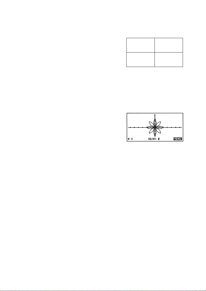
Parametric
Example
Plot the expressions from the previous Parametric example,
x(f) = 3 sinSi and y(i) = 2 sin4f .Before plotting, however,
reset the default plot settings by clearing the Plot Setup view.
I Select Parametric
{{START}}
Make sure the correct function
is highlighted and checked,
m [SETUP-PLOT]
■ [CLEAR]
T: 0
ibn:ih
PLOT
Polar Example
Plot the expression from the previous Polar example,
r = 2 cos40. Before plotting, however, reset the default plot
settings by clearing the Plot Setup view.
j Select Polar
{{START}}
Make sure the correct function
is highlighted and checked.
■ [SETUP-PLOT]
■ [CLEAR]
PLOT
Plotting and Exploring Functions 3-9
Page 74

Sequence Plot the Fibonacci sequence from the previous Sequence
Example example, i/, = 1, = 1, and = i/„_, + . In Plot Setup,
first set the SEQPLOT to Stairstep, then try a Cobweb plot.
Reset the default plot settings by clearing the Plot Setup view.
® A Stairstep graph plots n on the horizontal axis and t/ on
the vertical axis.
e A Cobweb graph plots on the horizontal axis and
on the vertical axis.
I LIB I Select Sequence
{{START}}
Make sure the correct function
is highlighted and checked.
SEQUENCE PLOT SETUP
SECFLDT: ISUEEfaSUEfS
NRNQ: 1
XRNQ: -2
VRNG; -2
CHQD^E SEQUENCE PLOT TVPE
24
24
10.6
■ {SETUP-PLOT]
m [CLEAR]
PLOT
Now set SEQPLOT to Cobweb and see the difference.
m [SETUP-PLOT]
{{CHOOS}}
Select Cobweb
PLOT
3-10 Plotting and Exploring Functions
Page 75

Exploring the Plot
Plot view (press [ plot | or ■ [VIEWS]) gives you a selection
of menu keys to explore a graph further (for the checkmarked
expressions in the Symbolic view). The options vary from
aplet to aplet.
PLOT View
Keys
Key
■ [CLEAR]
■ [VIEWS]
■ a
■ 0
([ZOOM]}
([TRACE]}
{{(X,Y)}}
({FCN}}
([DEFN]}
({MENU}}
Meaning
Erases the plot.
Offers additional pre-defined views for
splitting the screen and for scaling
(“zooming") the axes.
Moves cursor to far left or far right.
Displays ZOOM menu list.
Turns Trace mode on/off. The ■ appears
when Trace mode is on ({{trac*}}).
Displays the cursor’s coordinate position.
Press {{MENU}} to restore the menu.
Function aplet only: Turns on menu list for
root-finding functions (see “Interactive Root-
Finding, ’’ later in this chapter}.
Displays the current, defining expression.
Press {{MENU}} to restore the menu.
Turns menu-key labels on and off. When the
labels are off, any top-row key turns them
back on.
Plotting and Exploring Functions 3-11
Page 76

Tracing
Many aplets have a Trace mode. Trace mode is on when a
plot has just been drawn. When Trace mode is on, the
crosshairs cursor follows just the plotted points when you
press the Q or @ keys. The cursor traces the function. The
display also shows the current coordinate position (jc, y) of
the cursor.
If there is more than one curve displayed, press (T| or [Yl to
move between curves.
Note that tracing might not appear to exactly follow your plot
if the resolution (in Plot Setup view) is set to Faster. This is
because RES: FASTER plots in only every other column,
whereas tracing always uses every column.
In Function and Sequence Aplets : You can also scroll
(move the cursor) left or right beyond the edge of the display
window in Trace mode, giving you a view of more of the plot.
crosshairs
cursor
coordinates.
: FSiinn
3-12 Plotting and Exploring Functions
Page 77

To turn on e Trace mode and the coordinate display are automatically
TRACE mode set when a plot is drawn. At other times, set Trace mode by
pressing {{TRACE}} to change the label to {{TRAC«}}. (If
the menu labels are not displayed, press {{MENU}} first.)
• Turn off Trace mode by changing the menu label back to
{{TRACE}}.
To turn on e To turn On the display of the coordinates' values at the
coordinates current cursor position, press {{(X, Y)}}. To turn the
coordinate display off again, press {{MENU}}.
Zooming
One of the menu key options in PLOT is {{zoom}}. Zooming
redraws the plot on a larger or smaller scale, or on a
heightened or widened scale. It is a shortcut for changing the
Plot Setup, and it does change those settings.
With the Set Factors option you can specify the factors that
determine the extent of zooming, and whether the zoom is
centered about the cursor.
Not all ZOOM options are available in all aplets.
Plotting and Exploring Functions 3-13
Page 78

{{ZOOMI}
Options
Select an option and press {{OK}}.
Option Meanine
Center Recenters the plot around the current
position of the crosshairs without changing
the scale.
Box...
Lets you draw a box to define the zoom
boundaries. Use the cursor keys to draw the
box, and press {{OK}} to zoom in (see
below).
In Divides horizontal and vertical scales by the
X-factor and Y-factor (in Set Factors, below).
For instance, if zoom factors are 4, then
zooming in results in 1/4 as many units
depicted per pixel.
Out Multiplies horizontal and vertical scales by
the X-factor and Y-factor (in Set Factors,
below).
X-Zoom In Divides horizontal scale only, using X-factor.
X-Zoom Out Multiplies horizontal scale only, using X-
factor.
Y-Zoom In
Y-Zoom Out
Divides vertical scale only, using Y-factor.
Multiplies vertical scale only, using Y-factor.
Square Changes the vertical scale to match the
horizontal scale.
Set Factors...
Sets the X-Zoom and Y-Zoom factors for
zooming (multiplying for Zoom Out,
dividing for Zoom In). Includes option to
recenter the plot before zooming.
Un-zoom Returns the display to the previous zoom.
3-14 Plotting and Exploring Functions
Page 79

To use Box The Box Zoom option lets you draw a box around the area
Zoom you want to zoom in on.
1. If necessary, press {{MENU}} to turn on the menu-key
labels.
2. Press {{ZOOM}} and select Box.. .
3. Position the crosshairs into one corner of the box-to-be.
Press {{OK}}.
4. Use the cursor keys (,
etc.) to drag two sides of a
box.
5. Press {{OK}} to zoom in on
the boxed area.
Plotting and Exploring Functions 3-15
Page 80

Other Views for Scaling and Splitting the Graph
Other Scales The preset viewing options (■ [VIEWS]) draw the plot using
certain pre-defined axis scales. This is a shortcut for changing
Plot Setup. For instance, if you have defined a trigonometric
function, then you could select Trig to plot your function on
a trigonometric scale.
[VIEWS]
Options
Select an option and press ([OK]).
Option Meaninfi
Plot-Detail Splits the screen into the plot and a close-up
(see the next topic).
Plot-Table Splits the screen into the plot and the data
table (see page 3-24).
Overlay Plot Plots the current expression(s) without
erasing any pre-existing plot(s).
Auto Scale Rescales the axes using autoscaling.
Decimal
Rescales both axes so each pixel = 0.1 unit.
Resets default values for XRNG (-6.5 to 6.5)
and YRNG (-3.1 to 3.2). (Not in Sequence
or Statistics.)
Integer Rescales horizontal axis only, making each
pbcel =1 unit.(Not in Sequence or Statistics.)
Trig
Rescales horizontal axis so 1 pixel =Tr/24
radian, 7.5°, or 8.'/3 grads; rescales vertical
axis so 1 pixel=0.1 unit. (Not in Sequence or
Statistics.)
3-16 Plotting and Exploring Functions
Page 81

Splitting the
Screen
The Split Screen view can give you two simultaneous views of
the plot.
1. Press ■ [VIEWS] . Select Plot-Detail and press {{OK}}.
The graph is plotted twice. You can now zoom in on the
right side.
2. Press {{MENU}}{{ZOOM}} to choose the Zoom method and
press {{OK}} or I ENTER ¡.This zooms the right side. Here is
an example of split screen with zoom in.
The Plot menu keys are available as for the full plot (for
tracing, coordinate display, equation display, and so
on).
■ 0] or ■ moves the cursor to the far left or far
right of the full plot.
The {{<--}} left-arrow menu key will convert the base
plot (left side) to the scale of the zoomed plot (right
side). (It does so by resetting the variables’ minimum
and maximum values in the Plot Setup.)
Overlaying
Plots
plot} . The left side takes over3. To un-split the screen, press
the whole screen.
If you would like to plot over an existing plot without erasing
that plot, then use ■ {VIEWS} Overlay Plot instead of
I PLOT I. Note that tracing follows only the current functions
from the current aplet.
Plotting and Exploring Functions S-17
Page 82

Setting Up the Plot (Plot Setup)
Press ■ [SETUP-PLOT] to define any of the settings shown in
the next two tables.
1. Use the arrow keys to move from field to field. Highlight
the field to edit.
• If there is a number to enter, type it in and press | enter |
or {{OK}}.
• If there is an option to choose, press {{CHOOS}},
highlight your choice, and press | enter | or {{ok}}. As a
shortcut to {{CHOOS}}, just highlight the field to change
and press to display and select the different
choices.
• If there is an option to turn on/off, press {{/CHK}} to
check or uncheck it.
2. Press {{PAGET}} to view more settings.
3. When done, press [plot] to view the new plot.
To reset
settings
{SETUP-PLOT}
Settings
To reset the default values for all plot settings, press
■ {CLEAR} in the Plot Setup view.
Field
XRNG, YRNG.
TRNG,
6RNG,
NRNG
RES
TSTEP , eSTEP
SEQPLOT
XTICK
YTICK
Meaning
For Function plot: Specifies the
minimum and maximum horizontal (X)
and vertical (Y) values for the plotting
window.
For Parametric, Polar, and Sequence
plots: Specifies the time (T), angle (0), or
index (N) values for the graph.
For Function plots: Resolution. "Faster"
plots in alternate pixel columns; "More
Detail" plots in every pixel column.
For Parametric and Polar plots:
intervals at which to use the independent
variable to calculate the function.
For Sequence plots: Stairstep or
Cobweb types.
Horizontal spacing for tickmarks.
Vertical spacing for tickmarks.
3-18 Plotting and Exploring Functions
Page 83

Second-Page Those items with space for a checkmark are settings you can
turn on or off. Press {{PAGET}} to display the second page.
SIMULT
INV. CROSS
CONNECT
LABELS Label the axes with XRNG and YRNG
AXES
GRID
Interactive Root-Finding
You can find roots, intersections, slopes, and areas for a
function in the Plot view of the Function aplet (and any
Function-based aplets). The {{FCN}} operations act on the
currently selected expression or on the graph being traced.
The results are saved in the variables Area, Extremum, Isect,
Root, and Slope, so you can do further calculations with these
results in the aplet or in Home.
If more than one function is being
plotted, plot them simultaneously
(otherwise sequentially).
When the crosshairs cross the plot, invert
those pixels that are overlapping.
Connect the plotted points. (Sequence
always connects them.)
values.
Draw the axes.
Draw grid points using XTICK and YTICK
spacing.
To use a 1. In Symbolic view in a Function aplet, select the expression
{{FCN}} (for Intersect, two expressions) whose curve you want to
operation study. Or trace the curve you want to study.
2. Position the cursor where you want it to be before pressing
{{FCN}}. If you cannot see the crosshairs, they might be on
the axes. Press 0 or 0 to move the cursor and make it
visible.
3. Press {{FCN}}, then select an operation from the menu list
and press {{OK}}.
4. To perform another operation, press {{MENU}} to turn the
menu-key labels back on.
Plotting and Exploring Functions S-19
Page 84

To move the
cursor
To change the starting position of the cursor after having
selected an operation, press {{MENU}}, move the cursor, and
re-select the FCN operation.
To clear
shading
To remove the shading produced by the AREA operation,
press I PLOT I to re-draw the plot.
FCN Operations
Root Select Root to find the root x-value nearest the crosshairs. If
no root is found, but only an extremum, then the result is
labeled EXTR: instead of root :. (The root-finder is also
used in the Solve aplet. See also “Interpreting Results,” in
chapter 4.) The resulting x-value is saved in a variable named
Root.
Extremum Select Extremum to find the maximum or minimum nearest
the crosshairs. This displays the coordinate values and moves
the crosshairs to the extremum. (This uses the derivative.)
The resulting value is saved in a variable named Extremum.
Slope Select slope to find the numeric derivative at the point
nearest the crosshairs. The result is saved in a variable named
Slope.
Area Select Area to find the numeric integral. (If there are two or
more expressions checkmarked, then you will be asked to
choose the second expression from a list that includes the x-
axis.) Select a starting point, then move the cursor to shade a
region between the curve and the x-axis (or another curve),
and between the starting point and the current position. The
shaded region will be between the two curves. The Area is
the signed value of the shaded area. Areas below the x-axis
are negative. The result is saved in a variable named Area.
Intersection Select intersection to find the intersection of two graphs
nearest the crosshairs. (You need to have at least two selected
expressions in Symbolic view.) Displays the coordinate values
and moves the crosshairs to the intersection. (Uses Solve
function.) The resulting x-value is saved in a variable named
Isect.
3-20 Plotting and Exploring Functions
Page 85

Examples: Root-Finding with Plots
These examples of the interactive root-finding operations use
the expression f(x) = jc^-1 in the Function aplet with default
plot settings.
Select the Function aplet.
SYMB
{{X}} ■ [^] □ 1 [¡EUR]
IFUNCTIDN fVHBDLIC VIEH
^FKX>=Xa-l
F2t;x> =
F3<X> =
F4<X) =
F5<X> =
ROOT
EXTREMUM
SLOPE
[SETUP-PLOT]
[CLEAR]
PLOT
{{MENU}] {{FCN}}
Select Root {{OK}}
The crosshairs started at (0, -1). The root nearest the
crosshairs is x = -1. The crosshairs have moved to ( -1,0).
{{MENU}} {{FCN}}
5efeci Extremum {{OK}}
{{MENU}} {{FCN}}
Sefeci Slope {{OK}}
■ VI
ftDDT: -1
,,,,vL/,,
EHTftM: <0,-D
1
/
,, ,v
The slope at the extremum (where the crosshairs are) is zero.
/
I8IJ!III
isuim
iaB;iii
Plotting and Exploring Functions 3-21
Page 86

AREA
You move the cursor to the starting point first, then shade the
area.
{{MENU}} {{FCN}}
Select Area. . . {{OK}}
{{OK}} to set starting point
Q 10 times
{{OK}}
The shaded area has a value of -0,666666666667 (to 12-digit
accuracy). It is negative because the region lies below the x-
axis.
Enter a second expression, f(x) = in Function aplet, and
find the intersection of it with f(x) =x‘-l.
Select the Function aplet
SYMB
{{X}} 3 I enter)
,, ^
SELECT END POINT
...........................
^Fl<:x>=xa-1
^F2CX>=X''3
F3(:x:)=
F4<x:>=
F5<X>=
Esnoanii
[/
r
\l
FUNCTION SVHiOLIC VIEM^
iHHiiBirang
RCTiroai
INTERSECT You must specify whether to find the intersection with the
second function or with the x-axis.
I PLOT I {{MENU}} {{FCN}}
Select Intersection
{{OK}}
Select the function F(X)=X''3
(not the x-axis) {{ok}}.
3-22 Plotting and Exploring Functions
,.A|
l-SECT:
1/
n
Page 87

Using a Table of Numbers
Display a Table of Numbers (Numeric View)
After entering and selecting (checkmarking) the expression
in the Symbolic view, press | num| to view a table of data
values for the independent (X, T, 0, or N) and dependent
variables. To adjust the initial value or step size, change the
Numeric Setup.
NUM View
Keys
Key
{{ZOOM}}
{{BIG}}
{{DEFN}}
Meaning
Displays ZOOM menu list.
Toggles between two character sizes.
Displays the defining function expression for
the highlighted column. To cancel this
display, press {{DEFb}}.
independent
variable
full display of
highlighted -
value
- X F3
tf
.1
.S
.3
.4
.5
9.98334166-:
М||||81ИНМ1—1
---------------------------------
(f
.3435303
.ЗВ4Ч1ВЭ
.4744355
t68E-2
laatriaragran—
' dependent
variable
The table adds columns for each additional expression that is
checkmarked in the Symbolic view.
Press {{DEFN}} to display the
expression that defines the
function in the highlighted
column.
X FI F2 F3
0
-1
.1
-.44
-.46
-.41
-.ВЧ
-.75
.001
.008
.037
.064
.135
.3
.3
.4
.5
SINCX:)
Hililgl—
A
ВЕЕПЕЕП
ТоткчУ
.3455303
.ЭВ441ВЗ
.4744355
Automatic You can enter any new value in the X column for the
Recalculation independent variable. When you then press | enter!. the
values for the dependent variables are recalculated, and the
entire table is regenerated with a new interval between X
values.
Plotting and Exploring Functions 3-23
Page 88

Exploring the Table of Numbers
Zooming
{{ZOOM}}
Options
Zooming redraws the table of numbers in greater or lesser
detail.
Option
In
Meaning
Decreases the intervals for the independent
variable so a narrower range is shown. Uses
the NUMZOOM factor in Numeric Setup.
Out Increases the intervals for the independent
variable so that a wider range is shown.
Uses the NUMZOOM factor in Numeric
Setup.
Decimal Changes intervals for the independent
variable to 0.1 unit. Starts at zero. (Shortcut
to changing NUMSTARTand NUMSTEP.)
Integer
Changes intervals for the independent
variable to 1 unit. Starts at zero. (Shortcut to
changing NUMSTEP.)
Trig
Changes intervals for independent variable
to tt/24 radian or 7.5 degrees or 8V3 grads.
Starts at zero.
Un-zoom Returns the display to the previous zoom.
The display on the right is a Zoom In of the display on the left.
X FI
^25 *
.15
.2
-.ццнз?s
-.цц
-.Ц7?5
-.Bfi
X FI
-.*i«îl311
-.RR
iH
-.RBB?11
.1135
-.RB?3HH
.11B?5
-.RB5BRS
.135
-.RBR3?5
.1
snnsii IB1HGS33I
3-24 Plotting and Exploring Functions
Page 89

Splitting the
Screen
The Split Screen view gives you two simultaneous views.
1. In the Symbolic view of the appropriate aplet, make sure
the function(s) you want are checkmarked.
2. Press ■[VIEWS}.
Select Plot-Table
and press {{OK}}.
3. The Q and 0 cursor keys move the crosshairs along the
plot; the view of the table adjusts itself. The Q and [V)
cursor keys move the crosshairs from one graph to
another.
4. To return to a full Numeric (or Plot) view, press | num| (or
I PLOT I).
Setting Up the Table (Numeric Setup)
Press ■ [SETUP-NUM] to define any of the settings shown in
the table below. To reset the default values for all table
settings, press ■ [CLEAR].
1. Use the arrow keys to move from field to field. Highlight
the field to edit.
• If there is a number to enter, type it in and press | enter |
or {{OK}}. To modify an existing number, press
{{EDIT}}.
• If there is an option to choose, press {{CHOOS}},
highlight your choice, and press | enter] or {{OK}}.
• Shortcut: Press the {{PLOT>}} menu key to copy
values from the Plot Setup into NUMSTART and
NUMSTEP.
Wli
1
/ 1
J
X FI
-.6BB66
-.BBHIE
-.10625
-!BiHi6
!hOEB5
.601575
IESHB13I1I
-.62B66
2. When done, press |num| to review the table of numbers.
To reset To reset the default values for all table settings, press
settings ■[CLEAR}.
Plotting and Exploring Functions 3-25
Page 90

SETUP-NUM
Screen
Field Meaning
NUMSTART
Where to start the independent variable’s
first value.
NUMSTEP
The size of the increment from one
independent variable value to the next.
NUMTYPE
Type of numeric table: Automatic or
Build Your Own. To build your own table,
you must type each independent value
into the table yourself.
NUMZOOM
Zoom factor (multiplies the scale for
Zoom Out, divides for Zoom In).
Building Your Own Table of Numbers
The default NUMTYPE is "Automatic", which fills the table
with data for regular intervals of the independent (X, T, 0, or
N) variable. With NUMTYPE "Build Your Own", you fill the
table yourself by typing in the independent-variable values
you want, and the dependent values are then calculated and
displayed.
To format a 1. Start with an expression defined (in Symbolic view) in the
table aplet of your choice.
2. In the Numeric Setup (■ [SETUP-NUM]), choose
NUMTYPE: Build Your Own.
3. Open the Numeric view (|num|). To clear existing data in
the table, press ■ [CLEAR].
4. Enter the independent values in the left-hand column.
Type in the number and press | enter |. You do not have to
enter them in order, because the ([SORT]} function can
rearrange them. To insert a number between two others,
use ([INS]}.
You enter
numbers into
the X column.
The defining — X^-l
expression |iHBMi:aBiiaiBBiEi33i
for FI.
IS
an
ISS
FI
FI entries are
generated
automatically.
3-26 Plotting and Exploring Functions
Page 91

To clear data Press ■ [CLEAR] to erase the data from a table.
“Build Your
Own” Keys
Key
{{EDIT}} Puts the highlighted independent value (X, T,
{{INS}}
{{SORT}}
{{BIG}}
{{DEFN}} Displays the defining function expression for
mo
Meanine
0, or N) into the edit line. After you edit the
number, press |enter].
Inserts a row of zero values at the position of
the highlight. Replace the zero by typing the
number you want and pressing | enter 1.
Automatically rearranges the left-hand
column into values in ascending (getting
larger) or descending (getting smaller)
order.
Toggles between two character sizes.
the highlighted column.
Deletes the highlighted row.
■ {CLEAR} Clears all data from the table.
Plotting and Exploring Functions 3-27
Page 92

More Examples
Function
Example
Plot the circle, = 13. Rearrange the equation to
y = . This must be entered as two expressions,
y = ^(l3-x') and y = .
I LIB I Se/ect Function
SYMB
[^[D 13 □ {{X}} [x3 2Q]
I ENTER I
EU [S 0 13 □ {{X}} [13
IFUNCTIDN SVMeaUC MIEH
<^Fl<X)=>ra3-X'*'2>
>/F2CX>=-Ta3-X''2>
F4CX>=
F5<X>= w
2Q] I ENTER I
■ [SETUP-PLOT]
(Check that the Plot settings
are the defaults—if not, press
■ [CLEAR] .J
FUNCTION PLOT SETUP
KRNG:
VRNG: -3. 1
¡¡TICK: 1 VTICK: 1
RES: Faster
ENTER MINIMUM HURIZDNTRL VALUE
■ 6.5
3.2
PLOT
H: 0 FiiX
\
/
): 3.S0SSS1 li!M!ll|
The calculator plots the two expressions of the conic plot
separately, sometimes producing a discontinuity in the graph.
Specify a finer resolution to minimize these discontinuities.
(The gaps are due to the sampling interval.)
■ [SETUP-PLOT]
ESS {{cHoos}}
SelectMor& Detail
FUNCTIPN FLOT SETUP
!if!NG" ”6« 5 6*5
VRNa: -3.1 3.2
KTICK: 1 VTICK: 1
RES: legUCTM
CHUaSE PLOT RESULUTIDN
3-28 Plotting and Exploring Functions
Page 93

Function
Example,
continued
PLOT
■ [SETUP-NUM]
(Check that the Numeric
settings are the defaults—if
not, press miClIAR].)
NUM
V
H: 0 FliK
^^FUNCTiDN NUMERIC fETUF
NUMSTflfiT: 0
NUMSTEP: . 1
NUMTVPE:
NUMZDDM: 4
X FI F2
0
3.fi05551
3.fiOH16H
3lS>130HB
3.5B3ERH
.5
3.S?i?lH
■■ 3.S0SS51 i8n;iii
flut. omat i c
-3.S055S
-3.eoHifi
-3.6
-3.5330H
-3.3B3E>;
-3.5?i«?l
.3
J
Plotting and Exploring Functions 3-29
Page 94

Parametric Plot the two sets of equations below that describe the paths of
Example two particles over time. Look at the interval between f = 0 and
i= 6.5 seconds.
I 5e/eci Parametric
■ [SETUP-SYMB]
Check that Radians is set.
*PftMMETIilC SVMEnUC SETUP»
ANGLE MEASURE:
CHUDSE ANGLE MEASURE
1 SYMB I 16 Q 3 0 ® (Z1 3
0 {{T}} [enterI
4 0 {{T}} 0 5 fENTERl
2 0 H0 ■ [te] 0 2 0
{{T}} flNTE^
G0 3 0
W 02
^PARAMETRIC SVMRDLIC MIEH^^
-'XKT> = 16/'3-8-^3*T
^Yl(T)=4»T-5
^X2<T>=2*SIH<ir/2«T)
^ Y2 < T > =-3*C0S < ir^ 2»T :>
0 {{T}} [enterI
PLOT
Yl
\ 1
X.
T: 0 CS.3333i3i3i3
Use the Numeric view to determine whether the particles ever
collide (that is, whether their paths cross at the same moment
in time). Compare the T values when X1=X2 and when Y1=Y2.
You can tell from the plot that the points of intersection are at
or near X=2 and Y=3. If T is the same at these points, then the
points collide.
NUM
Search for XI =2 and X2=2.
Move the highlight to
Xl=l.866666.
T XI Yl X2
3.3
3.333333
!§
Z.666666
1
3.H
1.1
1.3
3.133333
1.3
1.86666666666
wiiiiaB»IM««Maa№gigTdiBHI—
3,-sj liSMilip
-l.B
-l.H
-1
-.6
-.3
.3
1.303113
1.3753?fi
3
1.375376
1.303113
1.7B3013
You can see that X2=2 when T=1. Use ZOOM to home in on
Xl=2.
3-30 Plotting and Exploring Functions
Page 95

Parametric
Example,
continued
{{ZOOM}} Select in {{ok}}
as
T XI Y1
1.1?5 2.2 -.3 I.REH'IIO
l.S
ill:
1.3 .2
-.2 1.R02113
2.133333
-.1
0
iTIl'iil'l
.1
X2
1.B763B2
l.BHPPSR
I.BIBSBS
1.7B2013
1.99999999999
You can now see that Xl=2 when T=1.25, so the particles do
not collide at X=2.
Now search for Yl=3 and Y2=3. You can use {{ZOOM}} Out to
move more quickly through the columns, but {{ZOOM}} In
again to find Y1=Y2=3.
0 0 B highlight the Y2
column
to highlight Y2=3
T Y1
1.B75
l.R
l.RES
1.R5
l.R?S
2
3
Hililill
2.5
2.5
2.?
1:1
3
.3R01B05
.312B5BR
.2350?HB
.ISBRlBi
.07BS1R5
-22-11
X2
Y2
2.342356
2.463065
2.474205
2.440752
^u33£il£i
Since Y1 and Y2 intersect (when Y=3) at the same value for T,
the particles collide at T=2 seconds.
Plotting and Exploring Functions 3-31
Page 96

Polar Example Plot the circle, r = 3 (sin^e + cos^0).
I Select Polar
■ [SETUP^YMB]
Check that Radians is set.
ISYMB13 g El
M[A 0
miA 0
I cos I
enter!
{{6}} 0
{{6}} 0
PLOT
(If your plot does not look
this, check that the Plot Setup
has the default settings.)
^RK6>=3*c:SIN<0>a+C...
R2(;0> =
R3C0>=
R4i;0>=
R5<0>=
naEBEMiaKiiE
S: 0
fVMEDLIC VIEH^M
>: 3 rararni
gHihisirama
y
NUM
(If your table does not look
like this, make sure the
Numeric Setup has the default
settings.)
0
HHlilülB
R1
3
3
3
3
3
3
3-32 Plotting and Exploring Functions
Page 97

Sequence Generate a sequence to calculate the square root of 2 using
Example the iterative relationship
) X ) = \{Ul, +a), where a = 2.
Define this sequence in the HP 38G as
U1(N) = (Ul(N-iy + A)/(2*U1(N-1)) ,andstore2 in/t.
The Sequence aplet finds the square root by evaluating this
expression with successive values of N until the value for U1
stops changing. In this case, the sequence converges at a
value for -Jl starting with .
Start the sequence by setting U1 (1) and U1 (2) to 1.
I Select Sequence
{{START}}
11 ENTER I 1 [enter!
G]{{U1}}{{N-1}} ■ {X^} 0
^^SEOyENCE SYMEDLIC VIEM^
v^uia>=i
•/UK2>=1
v'Ul
usa:)=
U2<2>=
nail Banal
iBangmaB
0] 0 0 2 0 {{ui}}
{{N-1}} i)10^
Store the value 2 in the real variable A.
1 HOME I
2 {{STO^}} iA...Z|A I ENTER I
Set up a stairstep plot.
m {SETUP-PLOT]
Check that the default values
are set, including stairstep.
(Press ■ [CLEAR] to reset
default values.)
Plotting and Exploring Functions 3-33
SEQUENCE nOT SETUP
SEQPLDT: BWemWtggg
NRNQ: 1 24
XRNG; -2 24
TRNGi -2 10.6
CHOOSE SEQUENCE PLOT TVPE
Page 98

Sequence
Example,
continued
■ [VIEWS]
Select Auto Scale {{OK}}
Explore the graph and the
values for N and Ul by
pressing g and [^.
As you trace the graph with the cursor keys, the crosshairs
jump from N:1 to N:2 to N:3, and so on. The values for Ul
change by smaller and smaller amounts until they converge.
Ul
NUM
Scroll down to see that the
values for U] remain the same
for N»6. Therefore, -Jl is
N
a 1.5
H 1.415557
l.HlHilS
5
I.HIHBIH
$
8
1.41421356237
1.41421356237 to 12 digits of
accuracy.
Compare the Stairstep plot (which plots N and Ul (N)) to a
Cobweb plot (which plots Ul(N-l) and U1(N)). Use
autoscaling for the plot. The coordinate values and the
Numeric view are identical to the Stairstep plot.
■ {SETUP-PLOT} [3
Set SEQPLOT to Cobweb.
m {VIEWS}
Select Auto Scale {{OK}}
3-34 Plotting and Exploring Functions
Page 99
Solve
The Solve aplet will solve an equation or an expression for its
unknown variable. You define an equation or expression in
Symbolic view, then supply values for all of the variables
except one in Numeric view. Then Solve will find the
remaining unknown.
As a simple example, consider the equation
force = mass x acceleration (that is, f=m*a) in the Solve
Symbolic view.
SVMiaUC VliHS
^EliF=M*R
E3:
E4!
E5:
mia&sosi
If force is 600 N and acceleration is 9.8 m/sec^ then pressing
{{SOLV}} in the Solve Numeric view finds that the unknown
mass must be 61.22 kg.
1F: 600 1
ft: 9.8
NUMERIC SOLVE NUMERIC VIEW I
ft: 9.8
|F= 600 1
1.2244397959 ■
ENTER VALUE DR PRES! fDLVE
ENTER VALUE DR PRESS SOLVE
ntraimaTiHBaHHBBiTmnmTO
Furthermore, you can solve the equation for any one of its
variables. You can solve the equation as many times as you
want with new values and different unknowns.
Solve 4-1
Page 100

Solving Equations
An equation contains an equals sign. Its solution is a value for
the unkno^vn variable that makes both sides equal the same
value.
An expression does not contain an equals sign. Its solution is
a root, that is, a value for the unknown variable that makes the
expression equal to zero.
Define the Equation
You can define up to ten equations (or expressions), named
EO through E9. Each equation can contain up to 27 real
variables, named A through Z or 6.
To define an equation
1. In the Library ((u^), select the Solve aplet.
Display the Symbolic view (|symb|). If the highlight is on
2.
an existing equation, scroll to an empty line—unless you
don’t mind writing over the equation. Or, clear one line
(fpELl) or all lines (■ [CLEAR]).
Enter a complete equation, including the equals sign. (The
3.
equals sign is available as a menu key.) Use only A
through Z and 0 as variables’ names. Press | enter | or
{{OK}} to complete the equation. Only one equation at a
time can be checkmarked.
ISDLVE fVMiBLIC VIEH
^El;F=M*R
E3!
E4!
E5: *
A Solve variable (El through EO) can also be defined in terms
of other Solve variables. For instance, you could define El to
be the sum of E2 and E13.
4-2 Solve
 Loading...