

Page 1

ENGINEERING MANUAL of
AUTOMATIC
CONTROL
COMMERCIAL BUILDINGS
SI Edition
for
Page 2

Copyright 1989, 1995, and 1997 by Honeywell Inc.
All rights reserved. This manual or portions thereof may not be reporduced
in any form without permission of Honeywell Inc.
Library of Congress Catalog Card Number: 97-77856
Home and Building Control
Honeywell Inc.
Honeywell Plaza
P.O. Box 524
Minneapolis MN 55408-0524
Honeywell Latin American Region
480 Sawgrass Corporate Parkway
Suite 200
Sunrise FL 33325
Home and Building Control
Honeywell Limited-Honeywell Limitée
155 Gordon Baker Road
North York, Ontario
M2H 3N7
Honeywell Europe S.A.
3 Avenue du Bourget
1140 Brussels
Belgium
Printed in USA
ii
Honeywell Asia Pacific Inc.
Room 3213-3225
Sun Hung Kai Centre
No. 30 Harbour Road
Wanchai
Hong Kong
ENGINEERING MANUAL OF AUTOMATIC CONTROL
Page 3

FOREWORD
The Minneapolis Honeywell Regulator Company published the first edition of the Engineering Manual of
Automatic Control in l934. The manual quickly became the standard textbook for the commercial building
controls industry. Subsequent editions ha ve enjoyed ev en greater success in colleges, univ ersities, and contractor
and consulting engineering offices throughout the world.
Since the original 1934 edition, the building control industry has experienced dramatic change and made
tremendous advances in equipment, system design, and application. In this edition, microprocessor controls are
shown in most of the control applications rather than pneumatic, electric, or electronic to reflect the trends in
industry today. Consideration of configuration, functionality, and integration plays a significant role in the
design of building control systems.
Through the years Honeywell has been dedicated to assisting consulting engineers and architects in the
application of automatic controls to heating, ventilating, and air conditioning systems. This manual is an outgro wth
of that dedication. Our end user customers, the building owners and operators, will ultimately benef it from the
efficiently designed systems resulting from the contents of this manual.
All of this manual’s original sections have been updated and enhanced to include the latest developments in
control technology and use the International System of Units (SI). A ne w section has been added on indoor air
quality and information on district heating has been added to the Chiller, Boiler, and Distribution System
Control Applications Section.
This third SI edition of the Engineering Manual of Automatic Control is our contribution to ensure that we
continue to satisfy our customer’s requirements. The contr ib utions and encouragement receiv ed from pre vious
users are gratefully acknowledged. Further suggestions will be most welcome.
Minneapolis, Minnesota
December, 1997
KEVIN GILLIGAN
President, H&BC Solutions and Services
ENGINEERING MANUAL OF AUTOMATIC CONTROL
iii
Page 4

iv
ENGINEERING MANUAL OF AUTOMATIC CONTROL
Page 5

PREFACE
The purpose of this manual is to provide the reader with a fundamental understanding of controls and how
they are applied to the many parts of heating, ventilating, and air conditioning systems in commer cial buildings.
Many aspects of control are presented including air handling units, terminal units, chillers, boilers, building
airflow , water and steam distribution systems, smoke management, and indoor air quality . Control fundamentals,
theory, and types of controls provide background for application of controls to heating, ventilating, and air
conditioning systems. Discussions of pneumatic, electric, electronic, and digital controls illustrate that applications
may use one or more of several different control methods. Eng ineering data such as equipment sizing, use of
psychrometric charts, and conversion formulas supplement and support the control information. To enhance
understanding, definitions of terms are provided within individual sections.
Building management systems have ev olved into a major consideration for the control engineer when evaluating
a total heating, ventilating, and air conditioning system design. In response to this consideration, the basics of
building management systems configuration are presented.
The control recommendations in this manual are general in nature and are not the basis for any specific job or
installation. Control systems are furnished according to the plans and specifications prepared by the control
engineer. In many instances there is more than one control solution. Professional expertise and judgment are
required for the design of a control system. This manual is not a substitute for such expertise and judgment.
Always consult a licensed engineer for advice on designing control systems.
It is hoped that the scope of information in this manual will provide the readers with the tools to expand their
knowledge base and help develop sound approaches to automatic control.
ENGINEERING MANUAL OF AUTOMATIC CONTROL
v
Page 6

vi
ENGINEERING MANUAL OF AUTOMATIC CONTROL
Page 7

ENGINEERING MANUAL of
AUTOMATIC
CONTROL
CONTENTS
Foreward ............................................................................................................ iii
Preface ............................................................................................................ v
Control System Fundamentals .......................................................................................... 1
Control Fundamentals ............................................................................................................ 3
Introduction.......................................................................................... 5
Definitions............................................................................................ 5
HVAC System Characteristics ............................................................. 8
Control System Characteristics ........................................................... 15
Control System Components .............................................................. 30
Characteristics and Attributes of Control Methods .............................. 35
Psychrometric Chart Fundamentals ............................................................................................................ 37
Introduction.......................................................................................... 38
Definitions............................................................................................ 38
Description of the Psychrometric Chart............................................... 39
The Abridged Psychrometric Chart ..................................................... 40
Examples of Air Mixing Process.......................................................... 42
Air Conditioning Processes ................................................................. 43
Humidifying Process............................................................................ 44
Process Summary ............................................................................... 53
ASHRAE Psychrometric Charts .......................................................... 53
Pneumatic Control Fundamentals ............................................................................................................ 57
Introduction.......................................................................................... 59
Definitions............................................................................................ 59
Abbreviations....................................................................................... 60
Symbols............................................................................................... 61
Basic Pneumatic Control System ........................................................ 61
Air Supply Equipment.......................................................................... 65
Thermostats ........................................................................................ 69
Controllers ........................................................................................... 70
Sensor-Controller Systems ................................................................. 72
Actuators and Final Control Elements................................................. 74
Relays and Switches ........................................................................... 77
Pneumatic Control Combinations........................................................ 84
Pneumatic Centralization .................................................................... 89
Pneumatic Control System Example................................................... 90
Electric Control Fundamentals ............................................................................................................ 95
Introduction.......................................................................................... 97
Definitions............................................................................................ 97
How Electric Control Circuits are Classified ........................................ 99
Series 40 Control Circuits.................................................................... 100
Series 80 Control Circuits.................................................................... 102
Series 60 Two-Position Control Circuits............................................... 103
Series 60 Floating Control Circuits...................................................... 106
Series 90 Control Circuits.................................................................... 107
Motor Control Circuits.......................................................................... 114
ENGINEERING MANUAL OF AUTOMATIC CONTROL
vii
Page 8

Electronic Control Fundamentals ............................................................................................................ 119
Introduction.......................................................................................... 120
Definitions............................................................................................ 120
Typical System .................................................................................... 122
Components ........................................................................................ 122
Electronic Controller Fundamentals .................................................... 129
Typical System Application.................................................................. 130
Microprocessor-Based/DDC Fundamentals .................................................................................................... 131
Introduction.......................................................................................... 133
Definitions............................................................................................ 133
Background ......................................................................................... 134
Advantages ......................................................................................... 134
Controller Configuration ...................................................................... 135
Types of Controllers............................................................................. 136
Controller Software.............................................................................. 137
Controller Programming ...................................................................... 142
Typical Applications ............................................................................. 145
Indoor Air Quality Fundamentals ............................................................................................................ 149
Introduction.......................................................................................... 151
Definitions............................................................................................ 151
Abbreviations....................................................................................... 153
Indoor Air Quality Concerns ................................................................ 154
Indoor Air Quality Control Applications................................................ 164
Bibliography ......................................................................................... 170
Smoke Management Fundamentals ............................................................................................................ 171
Introduction.......................................................................................... 172
Definitions............................................................................................ 172
Objectives............................................................................................ 173
Design Considerations ........................................................................ 173
Design Priniples .................................................................................. 175
Control Applications ............................................................................ 178
Acceptance Testing ............................................................................. 181
Leakage Rated Dampers .................................................................... 181
Bibliography ......................................................................................... 182
Building Management System Fundamentals................................................................................................. 183
Introduction.......................................................................................... 184
Definitions............................................................................................ 184
Background ......................................................................................... 185
System Configurations ........................................................................ 186
System Functions................................................................................ 189
Integration of Other Systems............................................................... 196
viii
ENGINEERING MANUAL OF AUTOMATIC CONTROL
Page 9

Control System Applications .......................................................................................... 199
Air Handling System Control Applications...................................................................................................... 201
Introduction.......................................................................................... 203
Abbreviations....................................................................................... 203
Requirements for Effective Control...................................................... 204
Applications-General ........................................................................... 206
Valve and Damper Selection ............................................................... 207
Symbols............................................................................................... 208
Ventilation Control Processes ............................................................. 209
Fixed Quantity of Outdoor Air Control ................................................. 211
Heating Control Processes.................................................................. 223
Preheat Control Processes ................................................................. 228
Humidification Control Process ........................................................... 235
Cooling Control Processes.................................................................. 236
Dehumidification Control Processes ................................................... 243
Heating System Control Process ........................................................ 246
Year-Round System Control Processes .............................................. 248
ASHRAE Psychrometric Charts .......................................................... 261
Building Airflow System Control Applications ............................................................................................... 263
Introduction.......................................................................................... 265
Definitions............................................................................................ 265
Airflow Control Fundamentals ............................................................. 266
Airflow Control Applications................................................................. 280
References .......................................................................................... 290
Chiller, Boiler, and Distribution System Control Applications....................................................................... 291
Introduction.......................................................................................... 295
Abbreviations....................................................................................... 295
Definitions............................................................................................ 295
Symbols............................................................................................... 296
Chiller System Control......................................................................... 297
Boiler System Control.......................................................................... 327
Hot and Chilled Water Distribution Systems Control ........................... 335
High Temperature Water Heating System Control............................... 374
District Heating Applications................................................................ 380
Individual Room Control Applications ............................................................................................................ 395
Introduction.......................................................................................... 397
Unitary Equipment Control .................................................................. 408
Hot Water Plant Considerations .......................................................... 424
ENGINEERING MANUAL OF AUTOMATIC CONTROL
ix
Page 10

Engineering Information .......................................................................................... 425
Valve Selection and Sizing ............................................................................................................ 427
Introduction.......................................................................................... 428
Definitions............................................................................................ 428
Valve Selection .................................................................................... 432
Valve Sizing ......................................................................................... 437
Damper Selection and Sizing ............................................................................................................ 445
Introduction.......................................................................................... 447
Definitions............................................................................................ 447
Damper Selection................................................................................ 448
Damper Sizing..................................................................................... 457
Damper Pressure Drop ....................................................................... 462
Damper Applications ........................................................................... 463
General Engineering Data ............................................................................................................ 465
Introduction.......................................................................................... 466
Conversion Formulas and Tables ........................................................ 466
Electrical Data ..................................................................................... 473
Properties of Saturated Steam Data ................................................... 476
Airflow Data ......................................................................................... 477
Moisture Content of Air Data ............................................................... 479
Index .......................................................................................... 483
x
ENGINEERING MANUAL OF AUTOMATIC CONTROL
Page 11

SMOKE MANAGEMENT FUNDAMENTALS
CONTROL
SYSTEM
FUNDAMENTALS
ENGINEERING MANUAL OF AUTOMATIC CONTROL
1
Page 12

SMOKE MANAGEMENT FUNDAMENTALS
SMOKE MANAGEMENT FUNDAMENTALS
2
ENGINEERING MANUAL OF AUTOMATIC CONTROL
Page 13

CONTROL FUNDAMENTALS
Control Fundamentals
ENGINEERING MANUAL OF AUTOMATIC CONTROL
CONTENTS
Introduction ............................................................................................................ 5
Definitions ............................................................................................................ 5
HVAC System Characteristics ............................................................................................................ 8
General................................................................................................ 8
Heating ................................................................................................ 9
General ........................................................................................... 9
Heating Equipment ......................................................................... 10
Cooling ................................................................................................ 11
General ........................................................................................... 11
Cooling Equipment.......................................................................... 12
Dehumidification.................................................................................. 12
Humidification...................................................................................... 13
Ventilation ............................................................................................ 13
Filtration............................................................................................... 14
Control System Characteristics ............................................................................................................ 15
Controlled V ariables ............................................................................ 15
Control Loop........................................................................................ 15
Control Methods .................................................................................. 16
General ........................................................................................... 16
Analog and Digital Control .............................................................. 16
Control Modes ..................................................................................... 17
Two-Position Control ....................................................................... 17
General ....................................................................................... 17
Basic Two-Position Control ......................................................... 17
Timed Two-Position Control ........................................................ 18
Step Control .................................................................................... 19
Floating Control............................................................................... 20
Proportional Control ........................................................................ 21
General ....................................................................................... 21
Compensation Control ................................................................ 22
Proportional-Integral (PI) Control .................................................... 23
Proportional-Integral-Derivative (PID) Control ................................ 25
Enhanced Proportional-Integral-Derivative (EPID) Control............. 25
Adaptive Control.............................................................................. 26
Process Characteristics....................................................................... 26
Load ................................................................................................ 26
Lag .................................................................................................. 27
General ....................................................................................... 27
Measurement Lag....................................................................... 27
Capacitance................................................................................ 28
Resistance .................................................................................. 29
Dead Time .................................................................................. 29
Control Application Guidelines ............................................................ 29
ENGINEERING MANUAL OF AUTOMATIC CONTROL
3
Page 14

CONTROL FUNDAMENTALS
Control System Components ............................................................................................................ 30
Sensing Elements ............................................................................... 30
Temperature Sensing Elements...................................................... 30
Pressure Sensing Elements............................................................ 31
Moisture Sensing Elements ............................................................ 32
Flow Sensors .................................................................................. 32
Proof-of-Operation Sensors ............................................................ 33
Transducers......................................................................................... 33
Controllers ........................................................................................... 33
Actuators ............................................................................................. 33
Auxiliary Equipment............................................................................. 34
Characteristics and Attributes of Control Methods .............................................................................. 35
4
ENGINEERING MANUAL OF AUTOMATIC CONTROL
Page 15

INTRODUCTION
CONTROL FUNDAMENTALS
This section describes heating, ventilating, and air
conditioning (HV A C) systems and discusses characteristics and
components of automatic control systems. Cross-references are
made to sections that provide more detailed information.
A correctly designed HVAC control system can provide a
comfortable environment for occupants, optimize energy cost
and consumption, improve employee productivity, facilitate
efficient manufacturing, control smoke in the event of a fire,
and support the operation of computer and telecommunications
equipment. Controls are essential to the proper operation of
the system and should be considered as early in the design
process as possible.
Properly applied automatic controls ensure that a correctly
designed HVAC system will maintain a comfortable
environment and perform economically under a wide range of
operating conditions. Automatic controls regulate HVA C system
output in response to varying indoor and outdoor conditions to
maintain general comfort conditions in office areas and provide
narrow temperature and humidity limits where required in
production areas for product quality.
DEFINITIONS
Automatic controls can optimize HVAC system operation.
They can adjust temperatures and pressures automatically to
reduce demand when spaces are unoccupied and regulate
heating and cooling to provide comfort conditions while limiting
energy usage. Limit controls ensure safe operation of HVAC
system equipment and prevent injury to personnel and damage
to the system. Examples of limit controls are low-limit
temperature controllers which help prevent water coils or heat
exchangers from freezing and flow sensors for safe operation
of some equipment (e.g., chillers). In the event of a fire,
controlled air distribution can provide smoke-free evacuation
passages, and smoke detection in ducts can close dampers to
prevent the spread of smoke and toxic gases.
HVAC control systems can also be integra ted with security
access control systems, fire alarm systems, lighting control
systems, and building and facility management systems to
further optimize building comfort, safety, and efficiency.
The following terms are used in this manual. Figure 1 at the
end of this list illustrates a typical control loop with the
components identified using terms from this list.
Analog: Continuousl y variable (e.g., a faucet controlling water
from off to full flow).
Automatic contr ol system: A system that reacts to a change or
imbalance in the variable it controls by adjusting other
variables to restore the system to the desired balance.
Algorithm: A calculation method that produces a control output
by operating on an error signal or a time series of error
signals.
Compensation control: A process of automatically adjusting
the setpoint of a given controller to compensate for
changes in a second measured variable (e.g., outdoor
air temperature). For example, the hot deck setpoint
is normally reset upward as the outdoor air temperature
decreases. Also called “reset control”.
Control agent: The medium in which the manipulated variable
exists. In a steam heating system, the control agent is
the steam and the manipulated variable is the flow of
the steam.
Control point: The actual value of the controlled variable
(setpoint plus or minus offset).
Controlled medium: The medium in which the controlled
variable exists. In a space temperature control system,
the controlled variable is the space temperature and
the controlled medium is the air within the space.
Controlled V ariable: The quantity or condition that is measured
and controlled.
Controller: A device that senses changes in the controlled
variable (or receiv es input from a r emote sensor) and
derives the proper correction output.
Corrective action: Control action that results in a change of
the manipulated variable. Initiated when the controlled
variable deviates from setpoint.
Cycle: One complete e xecution of a repeatable process. In basic
heating operation, a cycle comprises one on period
and one off period in a two-position control system.
Cycling: A periodic change in the controlled v ariable from one
value to another. Out-of-control analog cycling is
called “hunting”. T oo frequent on-off c ycling is called
“short cycling”. Short cycling can harm electric
motors, fans, and compressors.
Cycling rate: The number of cycles completed per time unit,
typically cycles per hour for a heating or cooling system.
The inverse of the length of the period of the c ycle.
ENGINEERING MANUAL OF AUTOMATIC CONTROL
5
Page 16

CONTROL FUNDAMENTALS
Deadband: A range of the controlled variable in which no
corrective action is taken by the controlled system and
no energy is used. See also “zero energy band”.
Deviation: The difference between the setpoint and the value
of the controlled variable at any moment. Also called
“offset”.
DDC: Direct Digital Control. See also Digital and Digital
control.
Digital: A series of on and off pulses arranged to convey
information. Morse code is an early example.
Processors (computers) operate using digital language.
Digital control: A control loop in which a microprocessor-
based controller directly controls equipment based on
sensor inputs and setpoint parameters. The
programmed control sequence determines the output
to the equipment.
Droop: A sustained deviation between the control point and
the setpoint in a two-position control system caused
by a change in the heating or cooling load.
Enhanced proportional-integral-derivative (EPID) contr ol:
A control algorithm that enhances the standard PID
algorithm by allowing the designer to enter a startup
output value and error ramp duration in addition to
the gains and setpoints. These additional parameters
are configured so that at startup the PID output varies
smoothly to the control point with negligible overshoot
or undershoot.
Electric control: A control circuit that operates on line or low
voltage and uses a mechanical means, such as a
temperature-sensitive bimetal or bellows, to perf orm
control functions, such as actuating a switch or
positioning a potentiometer. T he controller signal usually
operates or positions an electric actuator or may switch
an electrical load directly or through a relay.
Electronic control: A control circuit that operates on low
voltage and uses solid-state components to amplify
input signals and perform control functions, such as
operating a relay or providing an output signal to
position an actuator. The controller usually furnishes
fixed control routines based on the logic of the solidstate components.
Final control element: A device such as a valve or damper
that acts to change the value of the manipulated
variable. Positioned by an actuator.
Hunting: See Cycling.
Load: In a heating or cooling system, the heat transfer that the
system will be called upon to provide. Also, the work
that the system must perform.
Manipulated variable: The quantity or condition regulated
by the automatic control system to cause the desired
change in the controlled variable.
Measured variable: A variable that is measured and may be
controlled (e.g., discharge air is measured and
controlled, outdoor air is only measured).
Microprocessor -based control: A control circuit that operates
on low voltage and uses a microprocessor to perform
logic and control functions, such as operating a relay
or providing an output signal to position an actuator.
Electronic devices are primarily used as sensors. The
controller often furnishes flexible DDC and energy
management control routines.
Modulating: An action that adjusts by minute increments and
decrements.
Offset: A sustained deviation between the control point and
the setpoint of a proportional control system under
stable operating conditions.
On/off control: A simple two-position control system in which
the device being controlled is either full on or full off
with no intermediate operating positions available.
Also called “two-position control”.
Pneumatic control: A control circuit that operates on air
pressure and uses a mechanical means, such as a
temperature-sensitive bimetal or bellows, to perform
control functions, such as actuating a nozzle and
flapper or a switching relay. The controller output
usually operates or positions a pneumatic actuator,
although relays and switches are often in the circuit.
Process: A gener al term that describes a change in a measurable
variable (e.g., the mixing of return and outdoor air
streams in a mixed-air control loop and heat transfer
between cold water and hot air in a cooling coil).
Usually considered separately from the sensing
element, control element, and controller.
Proportional band: In a proportional controller, the control
point range through which the controlled variable must
pass to move the final control element through its full
operationg range. Expressed in percent of primary
sensor span. Commonly used equivalents are
“throttling range” and “modulating range”, usually
expressed in a quantity of Engineering units (degrees
of temperature).
Lag: A delay in the effect of a changed condition at one point in
the system, or some other condition to which it is related.
Also, the delay in response of the sensing element of a
control due to the time required for the sensing element
to sense a change in the sensed variable.
Proportional control: A control algorithm or method in which
the final control element moves to a position
proportional to the deviation of the value of the
controlled variable from the setpoint.
6
ENGINEERING MANUAL OF AUTOMATIC CONTROL
Page 17
CONTROL FUNDAMENTALS
Proportional-Integral (PI) control: A control algorithm that
combines the proportional (proportional response) and
integral (reset response) control algorithms. Reset
response tends to correct the offset resulting from
proportional control. Also called “proportional-plusreset” or “two-mode” control.
Proportional-Integral-Derivative (PID) control: A control
algorithm that enhances the PI control algorithm by
adding a component that is proportional to the rate of
change (derivative) of the deviation of the controlled
variable. Compensates for system dynamics and
allows faster control response. Also called “threemode” or “rate-reset” control.
Reset Control: See Compensation Control.
Sensing element: A device or component that measures the
value of a variable.
Setpoint: The value at which the controller is set (e.g., the
desired room temperature set on a thermostat). The
desired control point.
Short cycling: See Cycling.
Step control: Control method in which a multiple-switch
assembly sequentially switches equipment (e.g.,
electric heat, multiple chillers) as the controller input
varies through the proportional band. Step controllers
may be actuator driven, electronic, or directly activ ated
by the sensed medium (e.g., pressure, temperature).
Throttling range: In a proportional controller, the control point
range through which the controlled variable must pass
to move the final control element through its full
operating range. Expressed in values of the controlled
variable (e.g., Kelvins or degrees Celsius, percent
relative humidity, kilopascals). Also called
“proportional band”. In a proportional room
thermostat, the temperature change required to drive
the manipulated variable from full off to full on.
Time constant: The time required for a dynamic component,
such as a sensor, or a control system to reach 63.2
percent of the total response to an instantaneous (or
“step”) change to its input. Typically used to judge
the responsiveness of the component or system.
Two-position control: See on/off control.
Zero energy band: An energy conservation technique that
allows temperatures to float between selected settings,
thereby preventing the consumption of heating or
cooling energy while the temperature is in this range.
Zoning: The practice of dividing a building into sections for
heating and cooling control so that one controller is
sufficient to determine the heating and cooling
requirements for the section.
MEASURED
VARIABLE
OUTDOOR
AIR
-2
OUTDOOR
AIR
CONTROLLED
MEASURED
VARIABLE
HOT WATER
RETURN
TEMPERATURE
MEDIUM
RESET SCHEDULE
15
-15
OA
CONTROLLED
VARIABLE
HOT WATER
SUPPLY
64
AUTO
55
90
HW
SETPOINT
CONTROL
POINT
HOT WATER
SUPPLY
TEMPERATURE
71
Fig. 1. Typical Control Loop.
70
SETPOINT
INPUT
PERCENT
OPEN
VALVE
SETPOINT
OUTPUT
41
FLOW
ALGORITHM IN
CONTROLLER
FINAL CONTROL
ELEMENT
STEAM
CONTROL
AGENT
MANIPULATED
VARIABLE
M15127
ENGINEERING MANUAL OF AUTOMATIC CONTROL
7
Page 18
CONTROL FUNDAMENTALS
HVAC SYSTEM CHARACTERISTICS
GENERAL
An HVAC system is designed according to capacity
requirements, an acceptable combination of first cost and operating
costs, system reliability, and available equipment space.
DAMPER
AIR
FILTER
COOLING
COIL
FAN
COOLING
TOWER
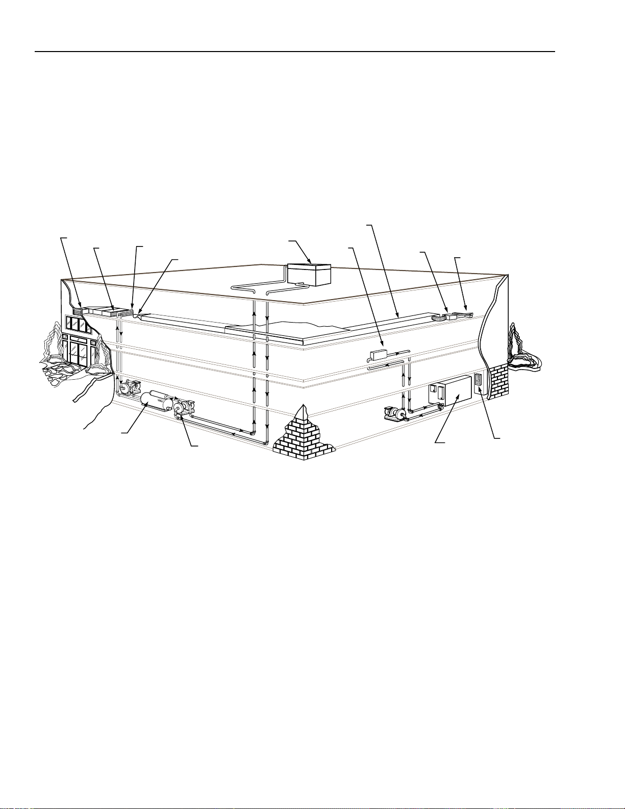
Figure 2 shows how an HVAC system may be distributed in
a small commercial building. The system control panel, boilers,
motors, pumps, and chillers are often located on the lower lev el.
The cooling tower is typically located on the roof. Throughout
the building are ductwork, fans, dampers, coils, air filters,
heating units, and variable air volume (VAV) units and dif fusers.
Larger buildings often hav e separate systems for groups of floors
or areas of the building.
DUCTWORK
HEATING
UNIT
VAV BOX
DIFFUSER
CHILLER
PUMP
Fig. 2. Typical HVAC System in a Small Building.
The control system for a commercial building comprises
many control loops and can be divided into central system and
local- or zone-control loops. For maximum comfort and
efficiency, all control loops should be tied together to share
information and system commands using a building
management system. Refer to the Building Management System
Fundamentals section of this manual.
BOILER
CONTROL
PANEL
M10506
The basic control loops in a central air handling system can
be classified as shown in Table 1.
Depending on the system, other controls may be required
for optimum performance. Local or zone controls depend on
the type of terminal units used.
8
ENGINEERING MANUAL OF AUTOMATIC CONTROL
Page 19
CONTROL FUNDAMENTALS
Table 1. Functions of Central HVAC Control Loops.
Control
Loop Classification Description
Ventilation Basic Coordinates operation of the outdoor, return, and exhaust air dampers to maintain
Better Measures and controls the volume of outdoor air to provide the proper mix of
Cooling Chiller control Maintains chiller discharge water at preset temperature or resets temperature
Cooling tower
control
Water coil control Adjusts chilled water flow to maintain temperature.
Direct expansion
(DX) system control
Fan Basic Turns on supply and return fans during occupied periods and cycles them as
Better Adjusts fan volumes to maintain proper duct and space pressures. Reduces system
Heating Coil control Adjusts water or steam flow or electric heat to maintain temperature.
Boiler control Operates burner to maintain proper discharge steam pressure or water temperature.
the proper amount of ventilation air. Low-temperature protection is often required.
outdoor and return air under varying indoor conditions (essential in variable air
volume systems). Low-temperature protection may be required.
according to demand.
Controls cooling tower fans to provide the coolest water practical under existing
wet bulb temperature conditions.
Cycles compressor or DX coil solenoid valves to maintain temperature. If
compressor is unloading type, cylinders are unloaded as required to maintain
temperature.
required during unoccupied periods.
operating cost and improves performance (essential for variable air volume systems).
For maximum efficiency in a hot water system, water temperature should be reset as
a function of demand or outdoor temperature.
HEATING
GENERAL
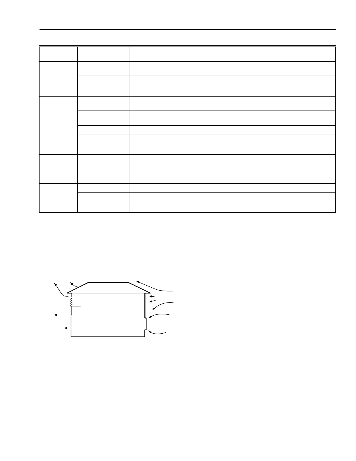
Building heat loss occurs mainly through transmission,
infiltration/exfiltration, and ventilation (Fig. 3).
TRANSMISSION
VENTILATION DUCT
EXFILTRATION
DOOR
Fig. 3. Heat Loss from a Building.
The heating capacity required for a building depends on the
design temperature, the quantity of outdoor air used, and the
physical activity of the occupants. Prevailing winds affect the
rate of heat loss and the degree of infiltration. The heating
system must be sized to heat the building at the coldest outdoor
temperature the building is likely to experience (outdoor design
temperature).
ROOF
20°C
-7°C
WINDOW
PREVAILING
WINDS
INFILTRATION
C3971
Transmission is the process by which energ y enters or leaves
a space through exterior surfaces. The rate of energy
transmission is calculated by subtracting the outdoor
temperature from the indoor temperature and multiplying the
result by the heat transfer coefficient of the surface materials.
The rate of transmission varies with the thickness and
construction of the exterior surfaces but is calculated the same
way for all exterior surfaces:
Energy Transmission per
Unit Area and Unit Time = (TIN - T
OUT
) x HTC
Where:
TIN= indoor temperature
T
= outdoor temperature
OUT
HTC = heat transfer coefficient
HTC
=
Unit Time x Unit Area x Unit Temperature
joule
ENGINEERING MANUAL OF AUTOMATIC CONTROL
9
Page 20
CONTROL FUNDAMENTALS
Infiltration is the process by which outdoor air enters a
building through walls, cracks around doors and windows, and
open doors due to the difference between indoor and outdoor
air pressures. The pressure differential is the result of
temperature difference and air intake or exhaust caused by f an
operation. Heat loss due to infiltration is a function of
temperature difference and volume of air moved. Exfiltration
is the process by which air leaves a building (e.g., through walls
and cracks around doors and windows) and carries heat with it.
Infiltration and exfiltration can occur at the same time.
Ventilation brings in fresh outdoor air that may require
heating. As with heat loss from inf iltration and exfiltration, heat
loss from ventilation is a function of the temperature difference
and the volume of air brought into the building or exhausted.
HEATING EQUIPMENT
Selecting the proper heating equipment depends on many
factors, including cost and availability of fuels, building size
and use, climate, and initial and operating cost trade-offs.
Primary sources of heat include gas, oil, wood, coal, electrical,
and solar energy . Sometimes a combination of sources is most
economical. Boilers are typically fueled by gas and may have
the option of switching to oil during periods of high demand.
Solar heat can be used as an alternate or supplementary source
with any type of fuel.
STEAM OR
HOT WATER
SUPPL Y
FAN
COIL
UNIT HEATER
STEAM TRAP
(IF STEAM SUPPLY)
CONDENSA TE
OR HOT WATER
RETURN
Fig. 5. Typical Unit Heater.
GRID PANEL
SERPENTINE PANEL
C2703
HOT WATER
SUPPL Y
HOT WATER
RETURN
HOT WATER
SUPPL Y
HOT WATER
RETURN
C2704
Figure 4 shows an air handling system with a hot water coil.
A similar control scheme would apply to a steam coil. If steam
or hot water is chosen to distribute the heat energy, highefficiency boilers may be used to reduce life-c ycle cost. Water
generally is used more often than steam to transmit heat energy
from the boiler to the coils or terminal units, because water
requires fewer safety measures and is typically more eff icient,
especially in mild climates.
THERMOSTAT
HOT WATER
SUPPLY
FAN
VALVE
HOT WATER
RETURN
DISCHARGE
AIR
C2702
Fig. 4. System Using Heating Coil.
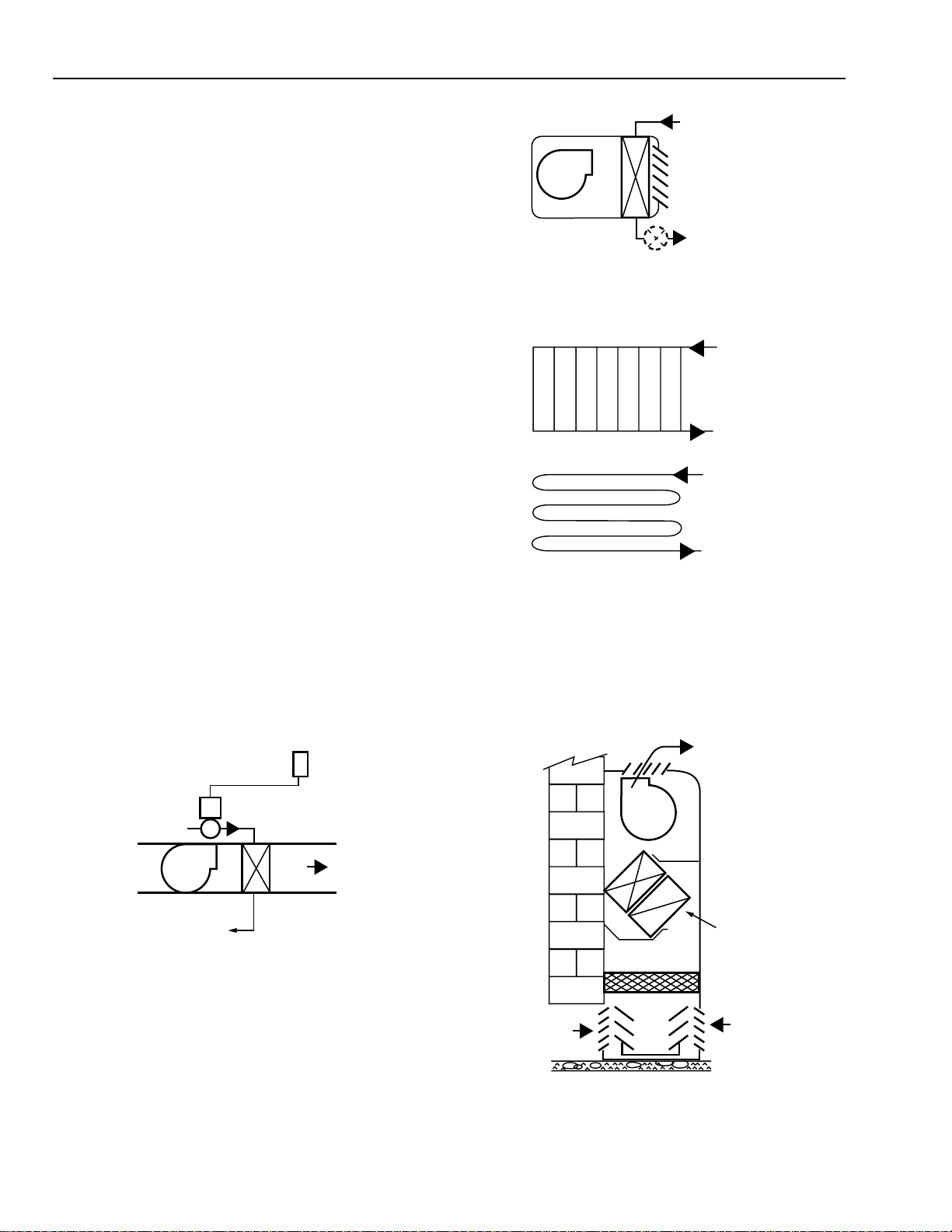
An air handling system provides heat by moving an air stream
across a coil containing a heating medium, across an electric
heating coil, or through a furnace. Unit heaters (Fig. 5) are
typically used in shops, storage areas, stairwells, and docks.
Panel heaters (Fig. 6) are typically used for heating floors and
are usually installed in a slab or floor structure, but may be
installed in a wall or ceiling.
Fig. 6. Panel Heaters.
Unit ventilators (Fig. 7) are used in classrooms and may
include both a heating and a cooling coil. Convection heaters
(Fig. 8) are used for perimeter heating and in entries and
corridors. Infrared heaters (Fig. 9) are typically used for spot
heating in large areas (e.g., aircraft hangers, stadiums).
FAN
DISCHARGE
AIR
COOLING
COIL
RETURN
AIR
C3035
WALL
OUTDOOR
AIR
HEATING
COIL
DRAIN PAN
MIXING
DAMPERS
Fig. 7. Unit Ventilator.
10
ENGINEERING MANUAL OF AUTOMATIC CONTROL
Page 21
CONTROL FUNDAMENTALS
FINNED TUBE
WARM AIR
RETURN AIR
SUPPLY
RETURN
FLOOR
TO OTHER
HEATING UNITS
FROM OTHER
HEATING UNITS
C2705
Fig. 8. Convection Heater.
REFLECTOR
INFRARED
SOURCE
RADIANT HEAT
C2706
Fig. 9. Infrared Heater.
In mild climates, heat can be provided by a coil in the central
air handling system or by a heat pump. Heat pumps have the
advantage of switching between heating and cooling modes as
required. Rooftop units provide packaged heating and cooling.
Heating in a rooftop unit is usually by a gas- or oil-fired furnace
or an electric heat coil. Steam and hot water coils are available
as well. Perimeter heat is often required in colder climates,
particularly under large windows.
A heat pump uses standard refrigeration components and a
reversing valv e to pro vide both heating and cooling within the
same unit. In the heating mode, the flow of refrigerant through
the coils is reversed to deliver heat from a heat source to the
conditioned space. When a heat pump is used to exchange heat
from the interior of a building to the perimeter, no additional
heat source is needed.
A heat-recovery system is often used in buildings where a
significant quantity of outdoor air is used. Several types of heatrecovery systems are av ailable including heat pumps, runaround
systems, rotary heat exchangers, and heat pipes.
In a runaround system, coils are installed in the outdoor air
supply duct and the exhaust air duct. A pump circulates the
medium (water or glycol) between the coils so that medium heated
by the exhaust air preheats the outdoor air entering the system.
A rotary heat exchanger is a large wheel filled with metal
mesh. One half of the wheel is in the outdoor air intake and the
other half, in the exhaust air duct. As the wheel r otates, the
metal mesh absorbs heat from the exhaust air and dissipates it
in the intake air.
A heat pipe is a long, sealed, finned tube charged with a
refrigerant. The tube is tilted slightly with one end in the outdoor
air intake and the other end in the exhaust air. In a heating
application, the refrigerant vaporizes at the lower end in the
warm exhaust air , and the vapor rises toward the higher end in
the cool outdoor air, where it gi v es up the heat of v aporization
and condenses. A wick carries the liquid refrigerant back to the
warm end, where the cycle repeats. A heat pipe requires no
energy input. For cooling, the process is rev ersed by tilting the
pipe the other way.
Controls may be pneumatic, electric, electronic, digital, or a
combination. Satisfactory control can be achieved using
independent control loops on each system. Maximum operating
efficiency and comfort levels can be achieved with a control
system which adjusts the central system operation to the
demands of the zones. Such a system can save enough in
operating costs to pay for itself in a short time.
Controls for the air handling system and zones are specifically
designed for a building by the architect, engineer, or team who
designs the building. The controls are usually installed at the job
site. T erminal unit controls are typically factory installed. Boilers,
heat pumps, and rooftop units are usually sold with a factoryinstalled control package specifically designed for that unit.
COOLING
GENERAL
Both sensible and latent heat contribute to the cooling load
of a building. Heat gain is sensible when heat is added to the
conditioned space. Heat gain is latent when moisture is added
to the space (e.g., by vapor emitted by occupants and other
sources). To maintain a constant humidity ratio in the space,
water vapor must be removed at a rate equal to its rate of addition
into the space.
Conduction is the process by which heat moves between
adjoining spaces with unequal space temperatures. Heat may
move through exterior walls and the roof, or through floors,
walls, or ceilings. Solar radiation heats surfaces which then
transfer the heat to the surrounding air. Internal heat gain is
generated by occupants, lighting, and equipment. Warm air
entering a building by infiltration and through ventilation also
contributes to heat gain.
Building orientation, interior and exterior shading, the angle
of the sun, and prevailing winds af fect the amount of solar heat
gain, which can be a major source of heat. Solar heat received
through windows causes immediate heat gain. Areas with large
windows may experience more solar gain in winter than in
summer. Building surf aces absorb solar energy , become heated,
and transfer the heat to interior air. The amount of change in
temperature through each layer of a composite surface depends
on the resistance to heat flow and thickness of each material.
Occupants, lighting, equipment, and outdoor air ventilation
and infiltration requirements contribute to internal heat gain.
For example, an adult sitting at a desk produces about 117 watts.
Incandescent lighting produces more heat than fluorescent
lighting. Copiers, computers, and other office machines also
contribute significantly to internal heat gain.
ENGINEERING MANUAL OF AUTOMATIC CONTROL
11
Page 22
CONTROL FUNDAMENTALS
COOLING EQUIPMENT
An air handling system cools by moving air across a coil
containing a cooling medium (e.g., chilled water or a
refrigerant). Figures 10 and 11 show air handling systems that
use a chilled water coil and a refrigeration evaporator (direct
expansion) coil, respectively. Chilled water control is usually
proportional, whereas control of an evaporator coil is twoposition. In direct expansion systems having more than one
coil, a thermostat controls a solenoid valve for each coil and
the compressor is cycled by a refrigerant pressure control. This
type of system is called a “pump down” system. Pump down
may be used for systems having only one coil, but more often
the compressor is controlled directly by the thermostat.
CHILLED
WATER
SUPPLY
TEMPERATURE
CONTROLLER
CONTROL
VALVE
CHILLED
WATER
COIL
SENSOR
CHILLED
WATER
RETURN
COOL AIR
C2707-2
Fig. 10. System Using Cooling Coil.
Compressors for chilled water systems are usually centrifugal,
reciprocating, or screw type. The capacities of centr ifugal and
screw-type compressors can be controlled by varying the
volume of refrigerant or controlling the compressor speed. DX
system compressors are usually reciprocating and, in some
systems, capacity can be controlled by unloading cylinders.
Absorption refrigeration systems, which use heat energy directly
to produce chilled water, are sometimes used for large chilled
water systems.
While heat pumps are usually direct expansion, a large heat
pump may be in the form of a chiller. Air is typically the heat
source and heat sink unless a large water reservoir (e.g., ground
water) is available.
Initial and operating costs are prime factors in selecting
cooling equipment. DX systems can be less expensive than
chillers. However, because a DX system is inherently twoposition (on/off), it cannot control temperature with the accuracy
of a chilled water system. Low-temperature control is essential
in a DX system used with a variable air volume system.
For more information control of various system equipment,
refer to the following sections of this manual:
— Chiller, Boiler, and Distribution System
Control Applications.
— Air Handling System Control Applications.
— Individual Room Control Applications.
TEMPERA TURE
CONTROLLER
EVAPORATOR
COIL
SOLENOID
VALVE
D
X
COOL AIR
SENSOR
REFRIGERANT
LIQUID
REFRIGERANT
GAS
C2708-1
Fig. 11. System Using Evaporator
(Direct Expansion) Coil.
Two basic types of cooling systems are available: chillers,
typically used in larger systems, and direct expansion (DX)
coils, typically used in smaller systems. In a chiller, the
refrigeration system cools water which is then pumped to coils
in the central air handling system or to the coils of fan coil
units, a zone system, or other type of cooling system. In a DX
system, the DX coil of the refrigeration system is located in
the duct of the air handling system. Condenser cooling for
chillers may be air or water (using a cooling tower), while DX
systems are typically air cooled. Because water cooling is more
efficient than air cooling, large chillers ar e always water cooled.
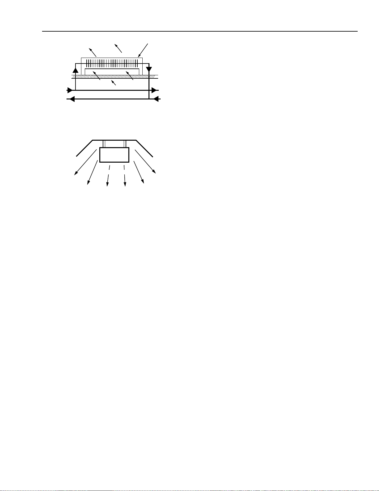
DEHUMIDIFICATION
Air that is too humid can cause problems such as condensation
and physical discomfort. Dehumidification methods circulate
moist air through cooling coils or sorption units.
Dehumidification is required only during the cooling season.
In those applications, the cooling system can be designed to
provide dehumidification as well as cooling.
For dehumidification, a cooling coil must have a capacity
and surface temperature sufficient to cool the air belo w its dew
point. Cooling the air condenses water, which is then collected
and drained away. When humidity is critical and the cooling
system is used for dehumidification, the dehumidified air may
be reheated to maintain the desired space temperature.
When cooling coils cannot reduce moisture content
sufficiently, sorption units are installed. A sorption unit uses
either a rotating granular bed of silica gel, activated alumina or
hygroscopic salts (Fig. 12), or a spray of lithium chloride brine
or glycol solution. In both types, the sorbent material absorbs
moisture from the air and then the saturated sorbent material
passes through a separate section of the unit that applies heat
to remove moisture. The sorbent material gi v es up moisture to
a stream of “scavenger” air , which is then exhausted. Scavenger
air is often exhaust air or could be outdoor air.
12
ENGINEERING MANUAL OF AUTOMATIC CONTROL
Page 23
CONTROL FUNDAMENTALS
HUMID
ROTATING
GRANULAR
BED
SORPTION
UNIT
AIR
DRY AIR
HUMID AIR
EXHAUST
HEATING
COIL
SCAVENGER
AIR
C2709
Fig. 12. Granular Bed Sorption Unit.
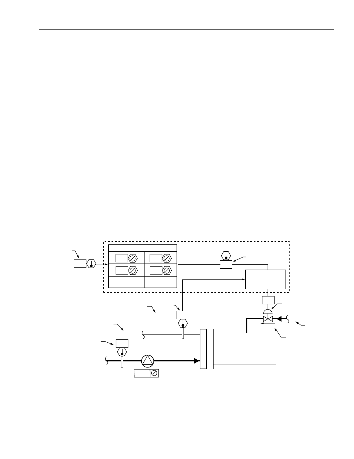
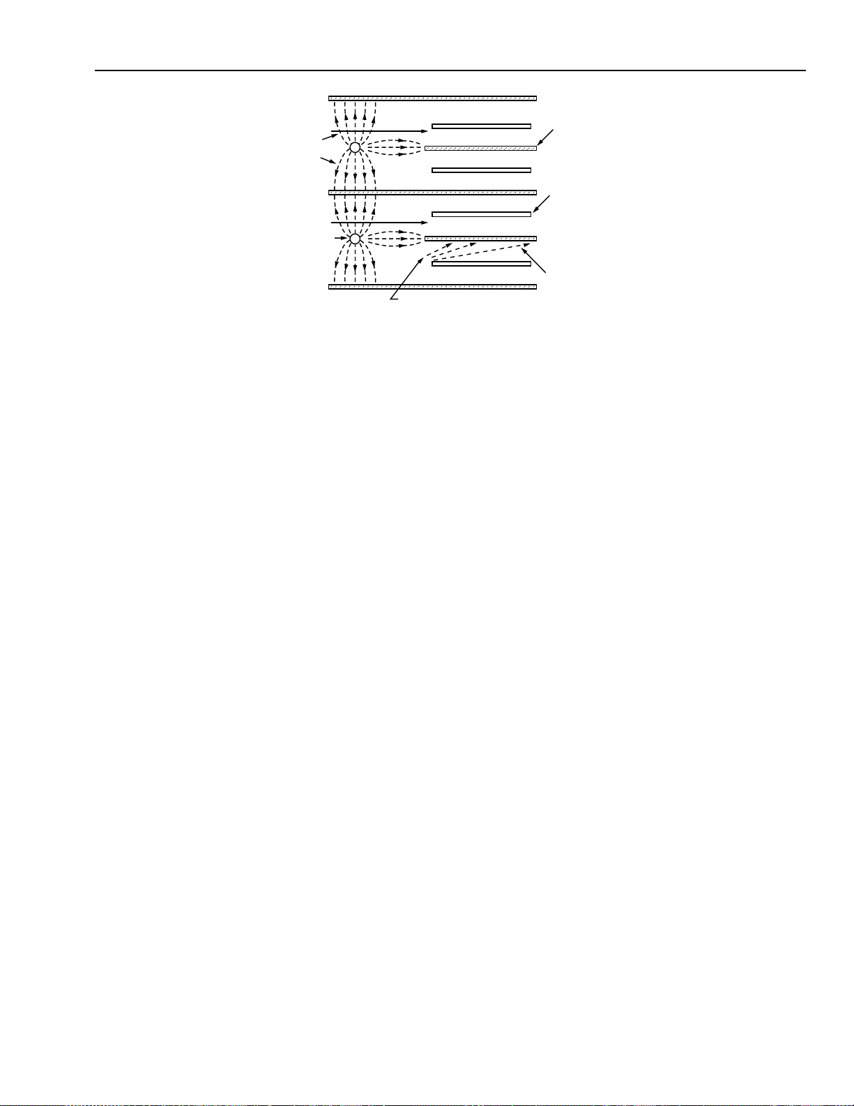
Sprayed cooling coils (Fig. 13) are often used for space humidity
control to increase the dehumidifier eff iciency and to provide yearround humidity control (winter humidification also).
MOISTURE
COOLING
COIL
ELIMINATORS
SPRAY
PUMP
M10511
Fig. 13. Sprayed Coil Dehumidifier.
For more information on dehumidification, refer to the
following sections of this manual:
— Psychrometric Chart Fundamentals.
— Air Handling System Control Applications.
VENTILATION
Ventilation introduces outdoor air to replenish the oxygen
supply and rid building spaces of odors and toxic gases.
Ventilation can also be used to pressurize a building to reduce
infiltration. While ventila tion is required in nearly all buildings,
the design of a ventilation system must consider the cost of
heating and cooling the ventilation air. Ventilation air must be
kept at the minimum required level except when used f or free
cooling (refer to ASHRAE Standard 62, Ventilation for
Acceptable Indoor Air Quality).
To ensure high-quality ventilation air and minimize the
amount required, the outdoor air intakes must be located to
avoid building exhausts, vehicle emissions, and other sources
of pollutants. Indoor exhaust systems should collect odors or
contaminants at their source. The amount of ventilation a
building requires may be reduced with air washers, high
efficiency f ilters, absorption chemicals (e.g., activ ated charcoal),
or odor modification systems.
Ventilation requirements vary according to the number of
occupants and the intended use of the space. For a breakdown
of types of spaces, occupancy levels, and required v entilation,
refer to ASHRAE Standard 62.
Figure 14 shows a ventilation system that supplies 100 percent
outdoor air. This type of ventilation system is typically used
where odors or contaminants originate in the conditioned space
(e.g., a laboratory where exhaust hoods and fans remove fumes).
Such applications require make-up air that is conditioned to
provide an acceptable environment.
EXHAUST
HUMIDIFICATION
Low humidity can cause problems such as respiratory
discomfort and static electricity. Humidifiers can humidify a
space either directly or through an air handling system. For
satisfactory environmental conditions, the relati ve humidity of
the air should be 30 to 60 percent. In critical areas where
explosive gases are present, 50 percent minimum is
recommended. Humidification is usually required only during
the heating season except in extremely dry climates.
Humidifiers in air handling systems typically inject steam
directly into the air stream (steam injection), spray atomized
water into the air stream (atomizing), or evaporate heated w ater
from a pan in the duct into the air stream passing through the
duct (pan humidification). Other types of humidifiers are a water
spray and sprayed coil. In spray systems, the water can be heated
for better vaporization or cooled for dehumidification.
For more information on humidification, refer to the following
sections of this manual:
— Psychrometric Chart Fundamentals.
— Air Handling System Control Applications.
SUPPLY
FAN
RETURN
AIR
MAKE-UP
AIR
SPACE
C2711
TO
OUTDOORS
OUTDOOR
AIR
SUPPLY
FILTER
EXHAUST
FAN
COIL
Fig. 14. Ventilation System Using
100 Percent Outdoor Air.
In many applications, energy costs make 100 percent outdoor
air constant volume systems uneconomical. For that reason,
other means of controlling internal contaminants are available,
such as variable volume fume hood controls, space
pressurization controls, and air cleaning systems.
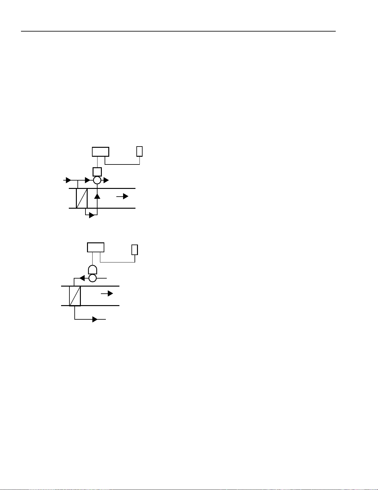
A ventilation system that uses return air (Fig. 15) is more
common than the 100 percent outdoor air system. The returnair ventilation system recirculates most of the return air from
the system and adds outdoor air for ventilation. The return-air
system may have a separate fan to overcome duct pressure
ENGINEERING MANUAL OF AUTOMATIC CONTROL
13
Page 24
CONTROL FUNDAMENTALS
losses. The exhaust-air system may be incorporated into the air
conditioning unit, or it may be a separate remote exhaust. Supply
air is heated or cooled, humidified or dehumidified, and
discharged into the space.
DAMPER RETURN FAN
EXHAUST
AIR
RETURN
AIR
FILTER COIL SUPPLY FAN
MIXED
AIR
SUPPLY
AIR
C2712
OUTDOOR
AIR
DAMPERS
Fig. 15. Ventilation System Using Return Air.
Ventilation systems as shown in Figures 14 and 15 should
provide an acceptable indoor air quality , utilize outdoor air for
cooling (or to supplement cooling) when possible, and maintain
proper building pressurization.
For more information on ventilation, refer to the following
sections of this manual:
— Indoor Air Quality Fundamentals.
— Air Handling System Control Applications.
— Building Airflow System Control Applications.
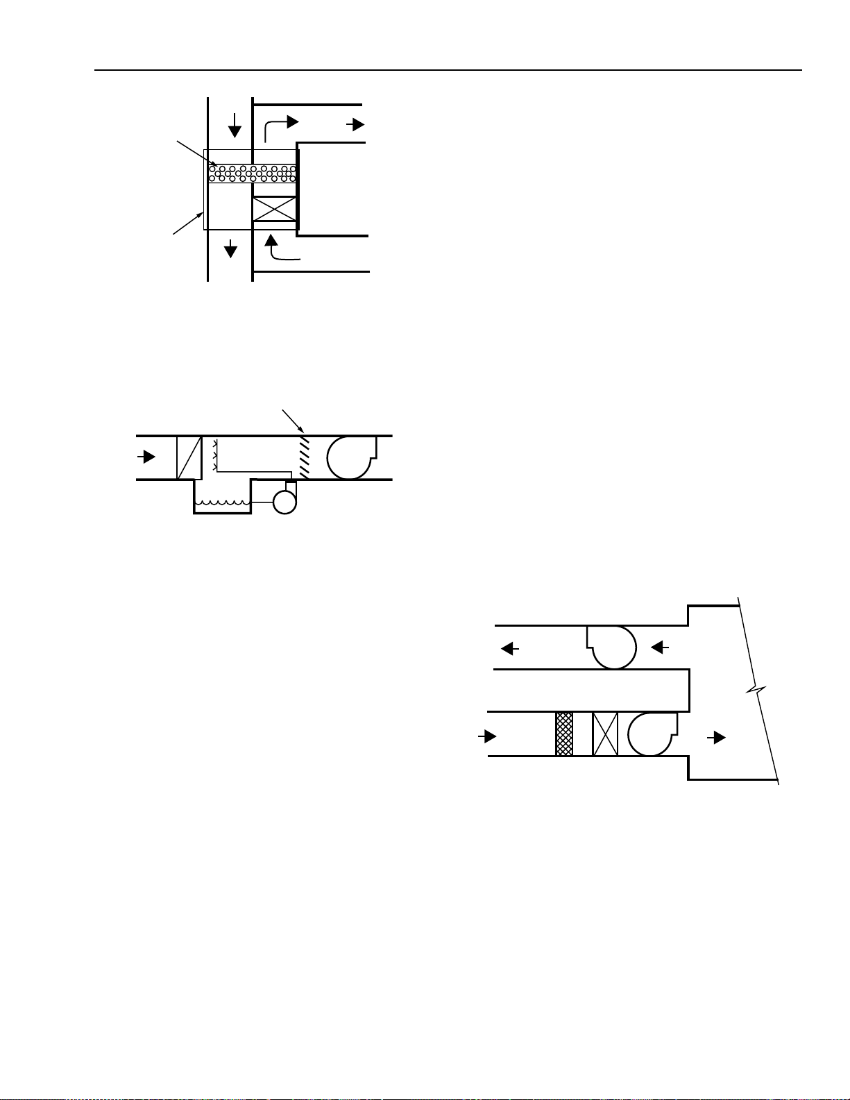
FILTRATION
Air filtration is an important part of the central air handling
system and is usually considered part of the ventilation system.
Two basic types of filters are available: mechanical filters and
electrostatic precipitation filters (also called electronic air
cleaners). Mechanical filters are subdivided into standard and
high efficiency.
PLEATED FILTER
Filters are selected according to the degree of cleanliness
required, the amount and size of particles to be removed, and
acceptable maintenance requirements. High-efficiency
particulate air (HEP A) mechanical filters (Fig. 16) do not release
the collected particles and therefore can be used for clean rooms
and areas where toxic particles are released. HEPA filters
significantly increase system pressure drop, which must be
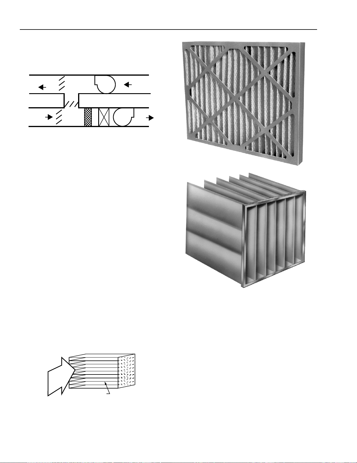
considered when selecting the fan. Figure 17 shows other
mechanical filters.
CELL
AIR FLOW
PLEATED PAPER
C2713
Fig. 16. HEPA Filter.
BAG FILTER
Fig. 17. Mechanical Filters.
Other types of mechanical filters include strainers, viscous
coated filters, and diffusion f ilters. Straining removes particles
that are larger than the spaces in the mesh of a metal filter and
are often used as prefilters for electrostatic filters. In viscous
coated filters, the particles passing through the filter fibers
collide with the fibers and are held on the fiber surface. Dif fusion
removes fine particles by using the turbulence present in the
air stream to drive particles to the fibers of the filter surface.
An electrostatic filter (Fig. 18) provides a low pressure drop
but often requires a mechanical prefilter to collect lar ge particles
and a mechanical after-filter to collect agglomerated particles
that may be blown off the electrostatic filter. An electrostatic
filter electrically charges particles passing through an ionizing
field and collects the charged particles on plates with an opposite
electrical charge. The plates may be coated with an adhesive.
14
ENGINEERING MANUAL OF AUTOMATIC CONTROL
Page 25
CONTROL FUNDAMENTALS
–
PATH
OF
IONS
WIRES
AT HIGH
POSITIVE
POTENTIAL
SOURCE: 1996 ASHRAE SYSTEMS AND EQUIPMENT HANDBOOK
AIRFLOW
AIRFLOW
POSITIVELY CHARGED
PARTICLES
Fig. 18. Electrostatic Filter.
CONTROL SYSTEM CHARACTERISTICS
Automatic controls are used wherever a variable condition
must be controlled. In HVAC systems, the most commonly
controlled conditions are pressure, temperature, humidity, and
rate of flow. Applications of automatic control systems range
from simple residential temperature regulation to precision
control of industrial processes.
CONTROLLED VARIABLES
The sensor can be separate from or part of the controller and
is located in the controlled medium. The sensor measures the
value of the controlled variable and sends the resulting signal
to the controller. The controller receives the sensor signal,
compares it to the desired value, or setpoint, and generates a
correction signal to direct the operation of the controlled device.
The controlled device varies the control agent to regulate the
output of the control equipment that produces the desired
condition.
+
ALTERNATE
PLATES
–
GROUNDED
+
–
INTERMEDIATE
PLATES
+
CHARGED
TO HIGH
POSITIVE
–
POTENTIAL
+
THEORETICAL
PATHS OF
–
CHARGES DUST
PARTICLES
C2714
Automatic control requires a system in which a controllable
variable exists. An automatic control system controls the
variable by manipulating a second variable. The second v ariable,
called the manipulated variable, causes the necessary changes
in the controlled variable.
In a room heated by air moving through a hot water coil, for
example, the thermostat measures the temperature (controlled
variable) of the room air (controlled medium) at a specified
location. As the room cools, the thermostat operates a valve
that regulates the flow (manipulated variable) of hot water
(control agent) through the coil. In this way, the coil furnishes
heat to warm the room air.
CONTROL LOOP
In an air conditioning system, the controlled variable is
maintained by varying the output of the mechanical equipment
by means of an automatic control loop. A control loop consists
of an input sensing element, such as a temperature sensor; a
controller that processes the input signal and produces an output
signal; and a final control element, such as a valve, that operates
according to the output signal.
HVAC applications use two types of control loops: open and
closed. An open-loop system assumes a fixed relationship
between a controlled condition and an external condition. An
example of open-loop control would be the control of perimeter
radiation heating based on an input from an outdoor air
temperature sensor. A circulating pump and boiler are energized
when an outdoor air temperature drops to a specified setting,
and the water temperature or flow is proportionally controlled
as a function of the outdoor temperature. An open-loop system
does not take into account changing space conditions from
internal heat gains, infiltration/exfiltration, solar gain, or other
changing variables in the building. Open-loop control alone
does not provide close control and may result in underheating
or overheating. For this reason, open-loop systems are not
common in residential or commercial applications.
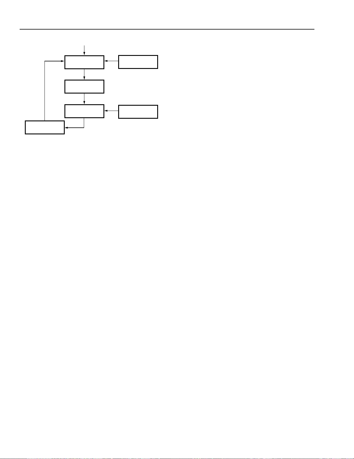
A closed-loop system relies on measurement of the controlled
variable to vary the controller output. Figure 19 sho ws a block
diagram of a closed-loop system. An example of closed-loop
control would be the temperature of discharge air in a duct
determining the flow of hot water to the heating coils to maintain
the discharge temperature at a controller setpoint.
ENGINEERING MANUAL OF AUTOMATIC CONTROL
15
Page 26
CONTROL FUNDAMENTALS
SETPOINT
FEEDBACK
SENSING
ELEMENT
CONTROLLER
CORRECTIVE
SIGNAL
FINAL CONTROL
ELEMENT
MANIPULATED
VARIABLE
PROCESS
CONTROLLED
VARIABLE
SECONDARY
INPUT
DISTURBANCES
C2072
Fig. 19. Feedback in a Closed-Loop System.
In this example, the sensing element measures the discharge
air temperature and sends a feedback signal to the controller.
The controller compares the feedback signal to the setpoint.
Based on the difference, or deviation, the controller issues a
corrective signal to a valve, which regulates the flow of hot
water to meet the process demand. Changes in the controlled
variable thus reflect the demand. The sensing element continues
to measure changes in the discharge air temperature and feeds
the new condition back into the controller for continuous
comparison and correction.
Automatic control systems use feedback to reduce the
magnitude of the deviation and produce system stability as
described above. A secondary input, such as the input from an
outdoor air compensation sensor, can provide information about
disturbances that affect the controlled variable. Using an input in
addition to the controlled variable enables the controller to
anticipate the effect of the disturbance and compensate for it, thus
reducing the impact of disturbances on the controlled variable.
CONTROL METHODS
GENERAL
An automatic control system is classified by the type of
energy transmission and the type of control signal (analog or
digital) it uses to perform its functions.
Self-powered systems are a comparatively minor but still
important type of control. These systems use the power of the
measured variable to induce the necessary corrective action.
For example, temperature changes at a sensor cause pressure
or volume changes that are applied directly to the diaphragm
or bellows in the valve or damper actuator.
Many complete control systems use a combination of the
above categories. An example of a combined system is the
control system for an air handler that includes electric on/off
control of the fan and pneumatic control for the heating and
cooling coils.
Various control methods are described in the following
sections of this manual:
— Pneumatic Control Fundamentals.
— Electric Control Fundamentals.
— Electronic Control Fundamentals.
— Microprocessor-Based/DDC Fundamental.
See CHARACTERISTICS AND ATTRIBUTES OF
CONTROL METHODS.
ANALOG AND DIGITAL CONTROL
Traditionally , analog de vices have performed HVA C control.
A typical analog HVAC controller is the pneumatic type which
receives and acts upon data continuously. In a pneumatic
controller, the sensor sends the controller a continuous
pneumatic signal, the pressure of which is proportional to the
value of the variable being measured. The controller compares
the air pressure sent by the sensor to the desired value of air
pressure as determined by the setpoint and sends out a control
signal based on the comparison.
The digital controller receives electronic signals from sensors,
converts the electronic signals to dig ital pulses (values), and
performs mathematical operations on these values. The
controller reconverts the output value to a signal to operate an
actuator. The controller samples digital data at set time intervals,
rather than reading it continually . The sampling method is called
discrete control signaling. If the sampling interval for the digital
controller is chosen properly, discrete output changes pr ovide
even and uninterrupted control performance.
The most common forms of energy for automatic control
systems are electricity and compressed air. Systems may
comprise one or both forms of energy.
Systems that use electrical energy are electromechanical,
electronic, or microprocessor controlled. Pneumatic control
systems use varying air pressure from the sensor as input to a
controller, which in turn produces a pneumatic output signal to
a final control element. Pneumatic, electromechanical, and
electronic systems perform limited, predetermined control
functions and sequences. Microprocessor-based controllers use
digital control for a wide variety of control sequences.
Figure 20 compares analog and digital control signals. The
digital controller periodically updates the process as a function
of a set of measured control variables and a giv en set of control
algorithms. The controller works out the entire computation,
including the control algorithm, and sends a signal to an actuator.
In many of the larger commercial control systems, an electronicpneumatic transducer conver ts the electric output to a v ariable
pressure output for pneumatic actuation of the final control
element.
16
ENGINEERING MANUAL OF AUTOMATIC CONTROL
Page 27

CONTROL FUNDAMENTALS
ANALOG CONTROL SIGNAL
OPEN
FINAL
CONTROL
ELEMENT
POSITION
CLOSED
OPEN
FINAL
CONTROL
ELEMENT
POSITION
CLOSED
DIGITAL CONTROL SIGNAL
TIME
TIME
C2080
Fig. 20. Comparison of Analog
and Digital Control Signals.
CONTROL MODES
Control systems use different control modes to accomplish
their purposes. Control modes in commercial applications
include two-position, step, and floating control; proportional,
proportional-integral, and proportional-integral-derivative
control; and adaptive control.
An example of differential gap would be in a cooling system
in which the controller is set to open a cooling valve when the
space temperature reaches 26°C, and to close the valve when
the temperature drops to 25°C. The difference between the two
temperatures (1°C or 1 Kelvin) is the differential gap. The
controlled variable fluctuates between the two temperatures.
Basic two-position control works well for many applications.
For close temperature control, however, the cycling must be
accelerated or timed.
Basic Tw o-Position Control
In basic two-position control, the controller and the final
control element interact without modification from a mechanical
or thermal source. The result is cyclical operation of the
controlled equipment and a condition in which the controlled
variable cycles back and forth between two v alues (the on and
off points) and is influenced by the lag in the system. The
controller cannot change the position of the final control element
until the controlled variable reaches one or the other of the two
limits of the differential. For that reason, the dif ferential is the
minimum possible swing of the controlled variable. Figure 21
shows a typical heating system cycling pattern.
TEMPERATURE
(°C)
23.5
OVERSHOOT
CONDTION
DIAL SETTING
DIFFERENTIAL
OFF
ON
23
22.5
22
21.5
21
TWO-POSITION CONTROL
General
In two-position control, the final control element occupies
one of two possible positions except for the brief period when
it is passing from one position to the other. T wo-position control
is used in simple HV A C systems to start and stop electric motors
on unit heaters, fan coil units, and refrigeration machines, to
open water sprays for humidification, and to energize and
deenergize electric strip heaters.
In two-position control, two values of the controlled variab le
(usually equated with on and off) determine the position of the
final control element. Between these values is a zone called the
“differential gap” or “differential” in which the controller cannot
initiate an action of the final control element. As the controlled
variable reaches one of the two values, the final control element
assumes the position that corresponds to the demands of the
controller, and remains there until the controlled variable
changes to the other value. The final control element mo v es to
the other position and remains there until the controlled variable
returns to the other limit.
20.5
20
TIME
UNDERSHOOT
CONDTION
C3972
Fig. 21. Typical Operation of Basic Two-Position Control.
The overshoot and undershoot conditions shown in Figure
21 are caused by the lag in the system. When the heating system
is energized, it builds up heat which moves into the space to
warm the air, the contents of the space, and the thermostat. By
the time the thermostat temperature reaches the off point (e.g.,
22°C), the room air is already warmer than that temperature.
When the thermostat shuts off the heat, the heating system
dissipates its stored heat to heat the space even more, causing
overshoot. Undershoot is the same process in reverse.
In basic two-position control, the presence of lag causes the
controller to correct a condition that has already passed rather
than one that is taking place or is about to take place. Consequently ,
basic two-position control is best used in systems with minimal
total system lag (including transfer, measuring, and f inal control
element lags) and where close control is not required.
ENGINEERING MANUAL OF AUTOMATIC CONTROL
17
Page 28
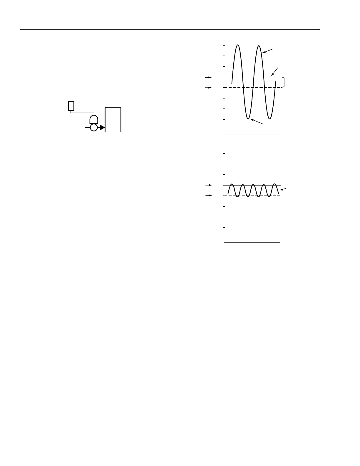
CONTROL FUNDAMENTALS
Figure 22 shows a sample control loop for basic two-position
control: a thermostat turning a furnace burner on or off in
response to space temperature. Because the thermostat cannot
catch up with fluctuations in temperature, overshoot and
undershoot enable the temperature to vary, sometimes
considerably. Certain industrial processes and auxiliary
processes in air conditioning have small system lags and can
use two-position control satisfactorily.
THERMOST AT
FURNACE
SOLENOID
GAS VALVE
C2715
Fig. 22. Basic Two-Position Control Loop.
Timed Tw o-Position Control
GENERAL
The ideal method of controlling the temperature in a space is
to replace lost heat or displace gained heat in exactly the amount
needed. With basic two-position control, such exact operation
is impossible because the heating or cooling system is either
full on or full off and the delivery at any specific instant is
either too much or too little. Timed two-position control,
however, anticipates requirements and delivers measured
quantities of heating or cooling on a percentage on-time basis
to reduce control point fluctuations. The timing is accomplished
by a heat anticipator in electric controls and by a timer in
electronic and digital controls.
In timed two-position control, the basic interaction between
the controller and the final control element is the same as for
basic two-position control. However, the controller responds
to gradual changes in the average value of the controlled v ariable
rather than to cyclical fluctuations.
Overshoot and undershoot are reduced or eliminated because
the heat anticipation or time proportioning feature results in a
faster cycling rate of the mechanical equipment. The result is
closer control of the variable than is possible in basic twoposition control (Fig. 23).
BASIC TWO-POSITION CONTROL
OVERSHOOT
CONDITION
DIAL SETTING
UNDERSHOOT
CONDITION
TIME
TIMED TWO-POSITION CONTROL
TIME
DIFFERENTIAL
CONTROL
POINT
C3973
TEMPERATURE
(°C)
OFF
ON
TEMPERATURE
(°C)
OFF
ON
23.5
23
22.5
22
21.5
21
20.5
20
23.5
23
22.5
22
21.5
21
20.5
20
Fig. 23. Comparison of Basic Two-Position
and Timed Two-Position Control.
HEAT ANTICIPATION
In electromechanical control, timed two-position control can
be achieved by adding a heat anticipator to a bimetal sensing
element. In a heating system, the heat anticipator is connected
so that it energizes whenev er the bimetal element calls for heat.
On a drop in temperature, the sensing element acts to turn on
both the heating system and the heat anticipator. The heat
anticipator heats the bimetal element to its off point early and
deenergizes the heating system and the heat anticipator . As the
ambient temperature falls, the time required for the bimetal
element to heat to the off point increases, and the cooling time
decreases. Thus, the heat anticipator automatically changes the
ratio of on time to off time as a function of ambient temperature.
18
ENGINEERING MANUAL OF AUTOMATIC CONTROL
Page 29
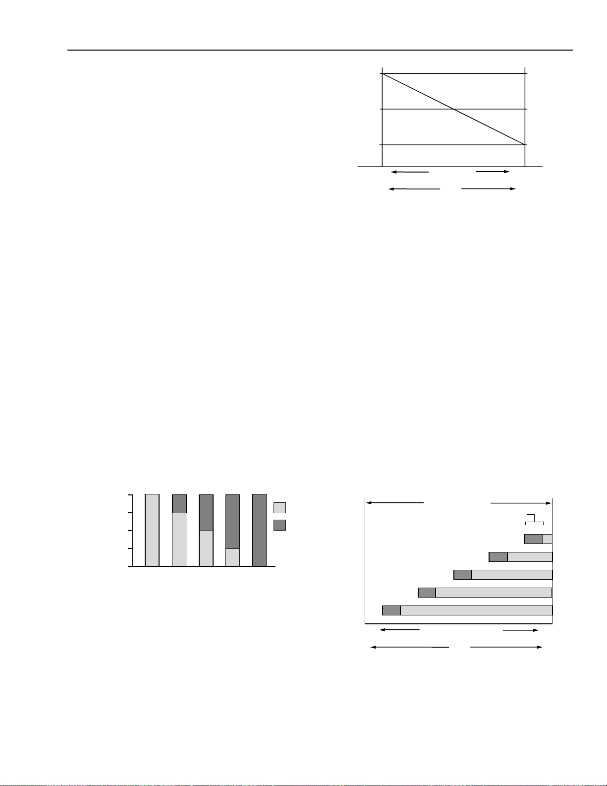
CONTROL FUNDAMENTALS
22.5
22
21.5
0
0.1
1
DROOP (°C)
CONTROL POINT (°C)
DESIGN
TEMPERATURE
OUTDOOR AIR
TEMPERATURE
0%
100%
LOAD
C3974
NO LOAD
TEMPERATURE
Because the heat is supplied to the sensor only, the heat
anticipation feature lowers the control point as the heat requirement
increases. The lowered control point, called “droop”, maintains a
lower temperature at design conditions and is discussed more
thoroughly in the following paragraphs. Energizing the heater
during thermostat off periods accomplishes anticipating action in
cooling thermostats. In either case, the percentage on-time varies
in proportion to the system load.
TIME PROPORTIONING
Time proportioning control provides more effective twoposition control than heat anticipation control and is available
with some electromechanical thermostats and in electronic and
Fig. 25. Relationship between Control Point,
Droop, and Load (Heating Control).
microprocessor-based controllers. Heat is introduced into the
space using on/off cycles based on the actual heat load on the
building and programmable time cycle settings. This method
reduces large temperature swings caused by a large total lag
and achieves a more even flow of heat.
Time proportioning control of two-position loads is
recommended for applications such as single-zone systems that
require two-position control of heating and/or cooling (e.g., a
gas-fired rooftop unit with direct-expansion cooling). Time
proportioning control is also recommended for electric heat
In electromechanical thermostats, the cycle rate is adjustable
by adjusting the heater. In electronic and digital systems, the
total cycle time and the minimum on and off times of the
controller are programmable. The total cycle time setting is
control, particularly for baseboard electric heat. With time
proportioning control, care must be used to avoid cycling the
controlled equipment more frequently than recommended by
the equipment manufacturer.
determined primarily by the lag of the system under control. If
the total cycle time setting is changed (e.g., from 10 minutes to
20 minutes), the resulting on/off times change accordingly (e.g.,
STEP CONTROL
from 7.5 minutes on/2.5 minutes off to 15 minutes on/5 minutes
off), but their ratio stays the same for a given load.
The cycle time in Figure 24 is set at ten minutes. At a 50
percent load condition, the controller, operating at setpoint,
produces a 5 minute on/5 minute off cycle. At a 75 percent
load condition, the on time increases to 7.5 minutes, the off
time decreases to 2.5 minutes, and the opposite cycle ratio
occurs at 25 percent load. All load conditions maintain the preset
10-minute total cycle.
10
ON
OFF
C2090
SELECTED
CYCLE TIME
(MINUTES)
7.5
5
2.5
0
100 75 50 25 0
LOAD (%)
Fig. 24. Time Proportioning Control.
Because the controller responds to average temperature or
humidity , it does not w ait for a cyc lic change in the controlled
variable before signaling correcti ve action. Thus control system
lags have no significant effect.
Droop in heating control is a lowering of the control point as
the load on the system increases. In cooling control, droop is a
Step controllers operate switches or relays in sequence to
enable or disable multiple outputs, or stages, of two-position
devices such as electric heaters or reciprocating refrigeration
compressors. Step control uses an analog signal to attempt to
obtain an analog output from equipment that is typically either
on or off. Figures 26 and 27 show that the stages may be
arranged to operate with or without overlap of the operating
(on/off) differentials. In either case, the typical two-position
differentials still exist but the total output is proportioned.
THROTTLING RANGE
DIFFERENTIAL
ONOFF
STAGES
5
4
3
2
1
ONOFF
23
ONOFF
SPACE TEMPERATURE (°C)
ONOFF
LOAD
ONOFF
22
100%0%
C3981
Fig. 26. Electric Heat Stages.
raising of the control point. In digital control systems, droop is
adjustable and can be set as low as one degree or even less.
Figure 25 shows the relationship of droop to load.
ENGINEERING MANUAL OF AUTOMATIC CONTROL
19
Page 30
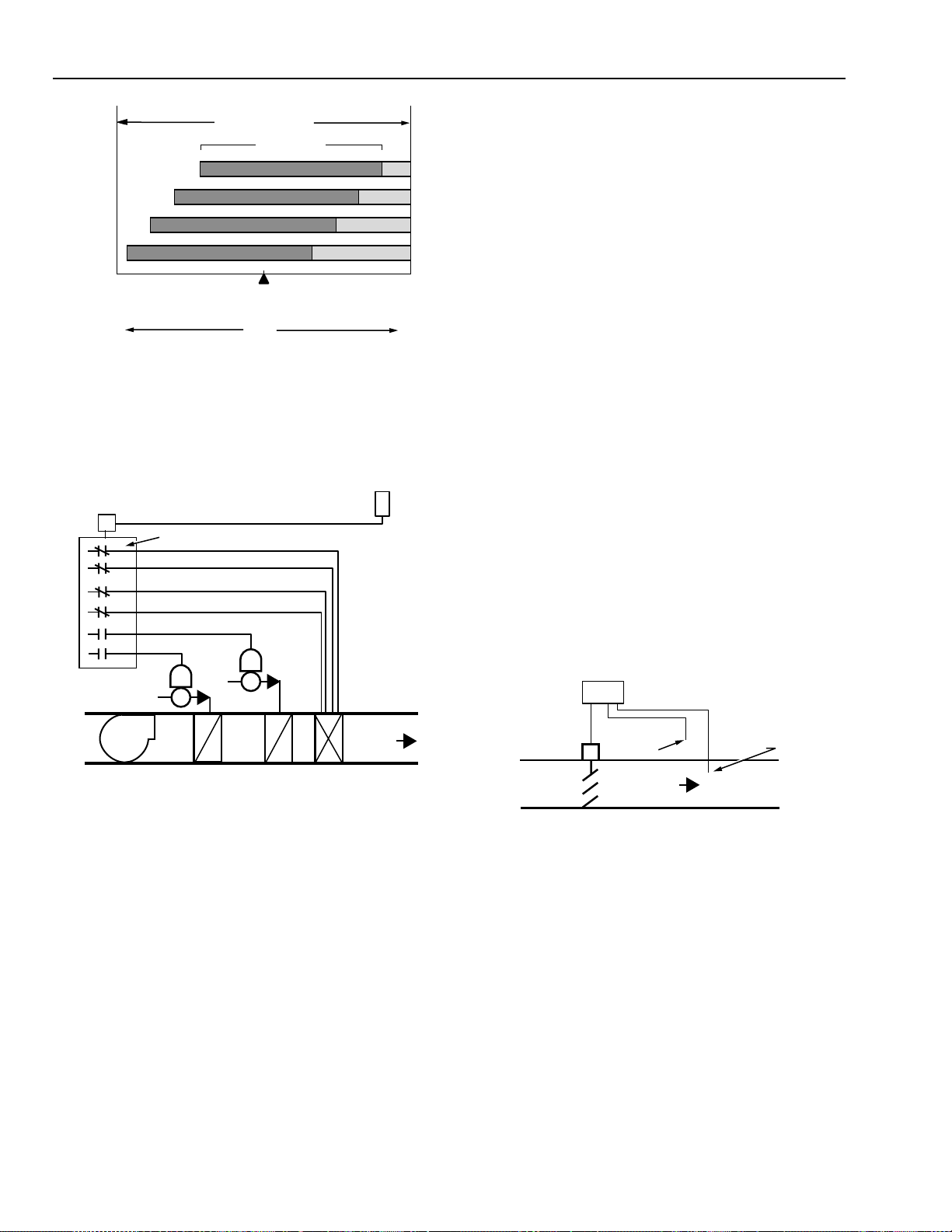
CONTROL FUNDAMENTALS
THROTTLING RANGE
STAGES
DIFFERENTIAL
4
3
2
OFF
1
22
SPACE TEMPERATURE (°C)
0%
23
SETPOINT
LOAD
ON
ONOFF
ONOFF
ONOFF
24
100%
C3982
Fig. 27. Staged Reciprocating Chiller Control.
Figure 28 shows step control of sequenced DX coils and electric
heat. On a rise in temperature through the throttling range at the
thermostat, the heating stages sequence off. On a further rise after
a deadband, the cooling stages turn on in sequence.
SPACE OR
ACTUATOR
6
5
4
3
2
1
STEP
CONTROLLER
FAN
STAGE NUMBERS
SOLENOID
VALVES
D
X
DIRECT EXPANSION
COILS
RETURN AIR
THERMOSTAT
D
X
MULTISTAGE
ELECTRIC HEAT
DISCHARGE
AIR
C2716
full on, the modulating stage returns to zero, and the sequence
repeats until all stages required to meet the load condition are on.
On a decrease in load, the process reverses.
With microprocessor controls, step control is usually done
with multiple, digital, on-off outputs since software allows
easily adjustable on-to-off per stage and interstage differentials
as well as no-load and time delayed startup and minimum on
and off adjustments.
FLOATING CONTROL
Floating control is a variation of two-position control and is
often called “three-position control”. Floating control is not a
common control mode, but is av ailable in most microprocessorbased control systems.
Floating control requires a slow-moving actuator and a fastresponding sensor selected according to the rate of response in
the controlled system. If the actuator should move too slowly,
the controlled system would not be able to keep pace with
sudden changes; if the actuator should move too quickly, twoposition control would result.
Floating control keeps the control point near the setpoint at
any load level, and can only be used on systems with minimal
lag between the controlled medium and the control sensor.
Floating control is used primarily for discharge control systems
where the sensor is immediately downstream from the coil,
damper, or device that it controls. An example of floating control
is the regulation of static pressure in a duct (Fig. 29).
FLOATING
STATIC
PRESSURE
CONTROLLER
ACTUATOR
REFERENCE
PRESSURE
PICK-UP
AIRFLOW
STATIC
PRESSURE
PICK-UP
Fig. 28. Step Control with Sequenced
DX Coils and Electric Heat.
A variation of step control used to control electric heat is
step-plus-proportional control, which provides a smooth
transition between stages. This control mode requires one of
the stages to be a proportional modulating output and the others,
two-position. For most efficient operation, the proportional
modulating stage should have at least the same capacity as one
two-position stage.
Starting from no load, as the load on the equipment increases,
the modulating stage proportions its load until it reaches full output.
Then, the first two-position stage comes full on and the modulating
stage drops to zero output and begins to proportion its output
again to match the increasing load. When the modulating stage
again reaches full output, the second two-position stage comes
DAMPER
C2717
Fig. 29. Floating Static Pressure Control.
In a typical application, the control point moves in and out
of the deadband, crossing the switch differential (Fig. 30). A
drop in static pressure below the controller setpoint causes the
actuator to drive the damper toward open. The narrow
differential of the controller stops the actuator after it has moved
a short distance. The damper remains in this position until the
static pressure further decreases, causing the actuator to drive
the damper further open. On a rise in static pressure above the
setpoint, the reverse occurs. Thus, the control point can float
between open and closed limits and the actuator does not move.
When the control point moves out of the deadband, the
controller moves the actuator toward open or closed until the
control point moves into the deadband again.
20
ENGINEERING MANUAL OF AUTOMATIC CONTROL
Page 31

CONTROL FUNDAMENTALS
22.5 23 23.5 24 24.5
100%
OPEN
50%
OPEN
CLOSED
POSITION OF FINAL
CONTROL ELEMENT
ACTUATOR
POSITION
CONTROL POINT (°C)
THROTTLING RANGE
C3983
ON
“CLOSE”
SWITCH
DIFFERENTIAL
SETPOINT
CONTROLLER
LOAD
DAMPER
POSITION
T1 T2 T3 T4 T5 T6
TIME
Fig. 30. Floating Control.
PROPORTIONAL CONTROL
General
Proportional control proportions the output capacity of the
equipment (e.g., the percent a valve is open or closed) to match
the heating or cooling load on the building, unlike two-position
control in which the mechanical equipment is either full on or
full off. In this way, proportional control achieves the desired
heat replacement or displacement rate.
OFF
DEADBAND
OFF
“OPEN”
ON
SWITCH
DIFFERENTIAL
C2094
CONTROL POINT
FULL LOAD
NO LOAD
OPEN
CLOSED
T7
In proportional control, the final control element moves to a
position proportional to the deviation of the value of the
controlled variable from the setpoint. The position of the f inal
control element is a linear function of the value of the controlled
variable (Fig. 32).
In a chilled water cooling system, for example (Fig. 31), the
sensor is placed in the discharge air. The sensor measures the
air temperature and sends a signal to the controller. If a
correction is required, the controller calculates the change and
sends a new signal to the valv e actuator. The actua tor repositions
the valve to change the water flow in the coil, and thus the
discharge temperature.
CONTROLLER
CHILLED
WATER
RETURN
AIR
VALVE
COIL
SENSOR
DISCHARGE
AIR
C2718
Fig. 31. Proportional Control Loop.
ENGINEERING MANUAL OF AUTOMATIC CONTROL
Fig. 32. Final Control Element Position as a
Function of the Control Point (Cooling System).
The final control element is seldom in the middle of its range
because of the linear relationship between the position of the
final control element and the value of the controlled varia ble.
In proportional control systems, the setpoint is typically the
middle of the throttling range, so there is usually an offset
between control point and setpoint.
21
Page 32

CONTROL FUNDAMENTALS
An example of offset would be the proportional control of a
chilled water coil used to cool a space. When the cooling load
is 50 percent, the controller is in the middle of its throttling
range, the properly sized coil valve is half-open, and there is
no offset. As the outdoor temperature increases, the room
temperature rises and more cooling is required to maintain the
space temperature. The coil valve must open wider to deliver
the required cooling and remain in that position as long as the
increased requirement exists. Because the position of the final
control element is proportional to the amount of deviation, the
temperature must deviate from the setpoint and sustain that
deviation to open the coil valve as far as required.
Figure 33 shows that when proportional control is used in a
heating application, as the load condition increases from 50
percent, offset increases toward cooler. As the load condition
decreases, offset increases toward warmer . The opposite occurs
in a cooling application.
WARMER
CONTROL POINT
SETPOINT
0%
LOAD
COOLER
OFFSET
50%
LOAD
OFFSET
C2096
100%
LOAD
Fig. 33. Relationship of Offset to
Load (Heating Application).
The throttling range is the amount of change in the controlled
variable required for the controller to move the controlled de vice
through its full operating range. The amount of change is
expressed in degrees kelvins for temperature, in percentages
for relative humidity , and in pascals or kilopascals for pressure.
For some controllers, throttling range is referred to as
“proportional band”. Proportional band is throttling range
expressed as a percentage of the controller sensor span:
Proportional Band =
Throttling Range
Sensor Span
x 100
Where:
V = output signal
K = proportionality constant (gain)
E = deviation (control point - setpoint)
M = value of the output when the deviation is
zero (Usually the output value at 50 percent
or the middle of the output range. The
generated control signal correction is added
to or subtracted from this value. Also called
“bias” or “manual reset”.)
Although the control point in a proportional control system
is rarely at setpoint, the offset may be acceptable. Compensation,
which is the resetting of the setpoint to compensate for varying
load conditions, may also reduce the effect of proportional offset
for more accurate control. An example of compensation is
resetting boiler water temperature based on outdoor air
temperature. Compensation is also called “reset control” or
“cascade control”.
Compensation Control
GENERAL
Compensation is a control technique available in proportional
control in which a secondary, or compensation, sensor resets
the setpoint of the primary sensor. An example of compensation
would be the outdoor temperature resetting the discharge
temperature of a fan system so that the discharge temperature
increases as the outdoor temperature decreases. The sample
reset schedule in Table 2 is shown graphically in Figure 34.
Figure 35 shows a control diagram for the sample reset system.
Table 2. Sample Reset Schedule.
Outdoor Air
Temperature
Condition
Outdoor design
(°C)
–20 40
temperature
Light load 20 20
Discharge Air
Temperature
(°C)
“Gain” is a term often used in industrial control systems for
the change in the controlled variable. Gain is the reciprocal of
proportional band:
Gain =
100
Proportional Band
The output of the controller is proportional to the deviation
of the control point from setpoint. A proportional controller
can be mathematically described by:
V = KE + M
40
(FULL RESET)
DISCHARGE AIR
20
TEMPERATURE SETPOINT (°C)
-20
(FULL
RESET)
OUTDOOR AIR TEMPERATURE (°C)
20
(RESET
START)
Fig. 34. Typical Reset Schedule for Discharge Air Control.
22
ENGINEERING MANUAL OF AUTOMATIC CONTROL
C3984
Page 33

CONTROL FUNDAMENTALS
OUTDOOR AIR
TEMPERATURE
SENSOR
RETURN
FAN
SENSOR
SUPPLY
TEMPERATURE
CONTROLLER
DISCHARGE
AIR
C2720
Fig. 35. Discharge Air Control Loop with Reset.
Compensation can either increase or decrease the setpoint as
the compensation input increases. Increasing the setpoint by
adding compensation on an increase in the compensation
variable is often referred to as positive or summer compensation.
Increasing the setpoint by adding compensation on a decrease
in the compensation variable is often referred to as negative or
winter compensation. Compensation is most commonly used
for temperature control, but can also be used with a humidity
or other control system.
Some controllers provide compensation start point capability .
Compensation start point is the value of the compensation
sensor at which it starts resetting the controller primary sensor
setpoint.
COMPENSA TION AUTHORITY
Compensation authority is the ratio of the effect of the
compensation sensor relative to the ef fect of the primary sensor.
Authority is stated in percent.
In an application requiring negativ e compensation, a change
in outdoor air temperature at the compensation sensor from –
18 to 16°C resets the hot water supply temperature (primary
sensor) setpoint from 94 to 38°C. Assuming a throttling r ange
of 7 Kelvins, the required authority is calculated as follows:
Authority =
Change in setpoint + TR
Change in compensation input
94 – 38 + 7
=
16 – (–18)
x 100
x 100
Authority = 185%
The previous example assumes that the spans of the two
sensors are equal. If sensors with unequal spans are used, a
correction factor is added to the formula:
Authority =
Compensation sensor span
Primary sensor span
Correction Factor
Change in setpoint ± TR
x
Change in compensation input
x 100
Assuming the same conditions as in the previous example, a
supply water temperature sensor range of 5 to 115°C (span of
110 Kelvins), an outdoor air temperature (compensation) sensor
range of -30 to 30°C (span of 60 Kelvins), and a throttling
range of 5 Kelvins, the calculation for negative reset would be
as follows:
60
Authority =
110
94 – 38 + 5
x
16 – (–18)
x 100
The basic equation for compensation authority is:
Authority =
Change in setpoint
Change in compensation input
x 100
For proportional controllers, the throttling range (TR) is
included in the equation. Two equations are required when the
throttling range is included. For direct-acting or positive reset,
in which the setpoint increases as the compensation input
increases, the equation is:
Authority =
Change in setpoint – TR
Change in compensation input
x 100
Direct-acting compensation is commonly used to prevent
condensation on windows by resetting the relative humidity
setpoint downward as the outdoor temperature decreases.
For reverse-acting or negative compensation, in which the
setpoint decreases as the compensation input increases, the
equation is:
Authority =
Change in setpoint + TR
Change in compensation input
x 100
Authority = 98%
The effects of throttling range may be disregarded with PI reset
controls.
PROPORTIONAL-INTEGRAL (PI) CONTR OL
In the proportional-integral (PI) control mode, reset of the
control point is automatic. PI control, also called “proportionalplus-reset” control, virtually eliminates offset and makes the
proportional band nearly invisible. As soon as the controlled
variable deviates abo ve or below the setpoint and offset de velops,
the proportional band gradually and automatically shifts, and the
variable is brought back to the setpoint. The major difference
between proportional and PI control is that proportional control
is limited to a single final control element position for each value
of the controlled variable. PI control changes the final control
element position to accommodate load changes while keeping
the control point at or very near the setpoint.
ENGINEERING MANUAL OF AUTOMATIC CONTROL
23
Page 34

CONTROL FUNDAMENTALS
The reset action of the integral component shifts the
proportional band as necessary around the setpoint as the load
on the system changes. The graph in Figure 36 shows the shift
of the proportional band of a PI controller controlling a normally
open heating valve. The shifting of the proportional band kee ps
the control point at setpoint by making further corrections in
the control signal. Because offset is eliminated, the proportional
band is usually set fairly wide to ensure system stability under
all operating conditions.
HEATING
VALVE
POSITION
CLOSED
50% OPEN
100% OPEN
0%
LOAD
34 37
= CONTROL POINT
THROTTLING RANGE = 5 KELVINS
50%
LOAD
PROPORTIONAL BAND
FOR SEPARATE LOAD
40
SETPOINT (°C)
CONDITIONS
100%
LOAD
43 46
C3985
Fig. 36. Proportional Band Shift Due to Offset.
Reset of the control point is not instantaneous. Whenever
the load changes, the controlled variable changes, producing
an offset. The proportional control makes an immediate
correction, which usually still leaves an offset. The integral
function of the controller then makes control corrections over
time to bring the control point back to setpoint (Fig. 37). In
addition to a proportional band adjustment, the PI controller
also has a reset time adjustment that determines the rate at which
the proportional band shifts when the controlled variable
deviates any given amount from the setpoint.
SETPOINT
DEVIATION
FROM
SETPOINT
CONTROL POINT (LOAD CHANGES)
OPEN
Reset error correction time is proportional to the deviation
of the controlled variable. For example, a four -percent deviation
from the setpoint causes a continuous shift of the proportional
band at twice the rate of shift for a two-percent deviation. Reset
is also proportional to the duration of the deviation. Reset
accumulates as long as there is offset, but ceases as soon as the
controlled variable returns to the setpoint.
With the PI controller, therefore, the position of the final
control element depends not only upon the location of the
controlled variable within the proportional band (proportional
band adjustment) but also upon the duration and magnitude of
the deviation of the controlled variable from the setpoint (reset
time adjustment). Under steady state conditions, the control
point and setpoint are the same for any load conditions, as shown
in Figure 37.
PI control adds a component to the proportional control
algorithm and is described mathematically by:
V = KE +
K
Edt + M
∫
T
1
Integral
Where:
V = output signal
K = proportionality constant (gain)
E = deviation (control point - setpoint)
T1= reset time
K/T1= reset gain
dt = differential of time (increment in time)
M = value of the output when the deviation
is zero
Integral windup, or an excessive overshoot condition, can
occur in PI control. Integral windup is caused by the integral
function making a continued correction while waiting for
feedback on the effects of its correction. While integral action
keeps the control point at setpoint during steady state conditions,
large overshoots are possible at start-up or during system upsets
(e.g., setpoint changes or large load changes). On many systems,
short reset times also cause overshoot.
Integral windup may occur with one of the following:
— When the system is off.
— When the heating or cooling medium fails or is not
available.
— When one control loop overrides or limits another.
VALVE
POSITION
INTEGRAL ACTION
PROPORTIONAL CORRECTION
T1 T2 T3 T4
TIME
Fig. 37. Proportional-Integral Control
Response to Load Changes.
CLOSED
C2098
Integral windup can be avoided and its effects diminished.
At start-up, some systems disable integral action until measured
variables are within their respectiv e proportional bands. Systems
often provide integral limits to reduce windup due to load
changes. The integral limits def ine the extent to which integral
action can adjust a device (the percent of full travel). The limit
is typically set at 50 percent.
24
ENGINEERING MANUAL OF AUTOMATIC CONTROL
Page 35

CONTROL FUNDAMENTALS
PROPORTIONAL-INTEGRAL-DERIVATIVE (PID)
CONTROL
Proportional-integral-derivative (PID) control adds the
derivative function to PI control. The derivative function
opposes any change and is proportional to the rate of change.
The more quickly the control point changes, the more corrective
action the derivative function provides.
If the control point moves away from the setpoint, the deri vative
function outputs a corrective action to bring the control point back
more quickly than through integral action alone. If the control
point moves toward the setpoint, the derivative function reduces
the corrective action to slow do wn the approach to setpoint, which
reduces the possibility of overshoot.
The rate time setting determines the effect of deriv ative action.
The proper setting depends on the time constants of the system
being controlled.
The derivative portion of PID control is expressed in the
following formula. Note that only a change in the magnitude
of the deviation can affect the output signal.
V = KT
dE
D
dt
Where:
V = output signal
K = proportionality constant (gain)
TD= rate time (time interval by which the
derivati ve advances the effect of
proportional action)
KTD= rate gain constant
dE/dt = derivative of the deviation with respect to
time (error signal rate of change)
The graphs in Figures 38, 39, and 40 show the effects of all
three modes on the controlled variable at system start-up. With
proportional control (Fig. 38), the output is a function of the
deviation of the controlled variable from the setpoint. As the
control point stabilizes, offset occurs. With the addition of
integral control (Fig. 39), the control point returns to setpoint
over a period of time with some degree of overshoot. The
significant difference is the elimination of of fset after the system
has stabilized. Figure 40 shows that adding the derivative
element reduces overshoot and decreases response time.
SETPOINT
CONTROL
POINT
T1 T2 T3 T4 T5 T6
TIME
OFFSET
C2099
Fig. 38. Proportional Control.
SETPOINT
CONTROL
T1 T2 T3 T4 T5 T6
TIME
POINT
OFFSET
C2100
Fig. 39. Proportional-Integral Control.
The complete mathematical expression for PID control
becomes:
V = KE + ∫Edt + KTD + M
T
1
dEK
dt
Proportional Integral Derivative
Where:
V = output signal
K = proportionality constant (gain)
E = deviation (control point - setpoint)
T1= reset time
K/T1= reset gain
dt = differential of time (increment in time)
TD= rate time (time interval by which the
derivati ve advances the effect of
proportional action)
KTD= rate gain constant
dE/dt = derivative of the deviation with respect to
time (error signal rate of change)
M = value of the output when the deviation
is zero
OFFSET
SETPOINT
T1 T2 T3 T4 T5 T6
TIME
C2501
Fig. 40. Proportional-Integral-Derivative Control.
ENHANCED PROPORTIONAL-INTEGRALDERIVATIVE (EPID) CONTROL
The startup overshoot, or undershoot in some applications,
noted in Figures 38, 39, and 40 is attributable to the very large
error often present at system startup. Microprocessor-based PID
startup performance may be greatly enhanced by exterior error
management appendages available with enhanced proportionalintegral-derivative (EPID) control. Two basic EPID functions
are start value and error ramp time.
ENGINEERING MANUAL OF AUTOMATIC CONTROL
25
Page 36

CONTROL FUNDAMENTALS
The start value EPID setpoint sets the output to a fixed v alue
at startup. For a VAV air handling system supply fan, a suitable
value might be twenty percent, a value high enough to get the
fan moving to prove operation to an y monitoring system and to
allow the motor to self cool. For a heating, cooling, and
ventilating air handling unit sequence, a suitable start value
would be thirty-three percent, the point at which the heating,
ventilating (economizer), and mechanical cooling demands are
all zero. Additional information is a vailable in the Air Handling
System Control Applications section.
The error ramp time determines the time duration during
which the PID error (setpoint minus input) is slowly ramped,
linear to the ramp time, into the PID controller. The controller
thus arrives at setpoint in a tangential manner without ov ershoot,
undershoot, or cycling. See Figure 41.
100
SETPOINT
START
PERCENT OPEN
VALUE
ACTUATOR POSITION
0
ERROR
RAMP
TIME
T1 T2 T3 T4 T5 T6
ELAPSED TIME
OFFSET
CONTROL
POINT
T7 T8
M13038
Fig. 41. Enhanced Proportional-
Integral-Derivative (EPID) Control.
ADAPTIVE CONTROL
Adaptive control is available in some microprocessor-based
controllers. Adaptive control algorithms enable a controller to
adjust its response for optimum control under all load
conditions. A controller that has been tuned to control accurately
under one set of conditions cannot always respond well when
the conditions change, such as a significant load change or
changeover from heating to cooling or a change in the velocity
of a controlled medium.
An adaptive control algorithm monitors the performance of
a system and attempts to improve the performance by adjusting
controller gains or parameters. One measurement of
performance is the amount of time the system requires to react
to a disturbance: usually the shorter the time, the better the
performance. The methods used to modify the gains or
parameters are determined by the type of adaptive algorithm.
Neural networks are used in some adaptive algorithms.
An example of a good application for adaptive control is
discharge temperature control of the central system cooling coil
for a VAV system. The time constant of a sensor varies as a
function of the velocity of the air (or other fluid). Thus the time
constant of the discharge air sensor in a VAV system is
constantly changing. The change in sensor response affects the
system control so the adaptive control algorithm adjusts system
parameters such as the reset and rate settings to maintain
optimum system performance.
Adaptive control is also used in energy management programs
such as optimum start. The optimum start program enables an
HVAC system to start as late as possible in the morning and still
reach the comfort range by the time the building is occupied for
the lease energy cost. To determine the amount of time required
to heat or cool the building, the optimum start program uses factors
based on previous building response, HVAC system
characteristics, and current weather conditions. The algorithm
monitors controller performance by comparing the actual and
calculated time required to bring the building into the comfort
range and tries to improve this performance by calculating new
factors.
PROCESS CHARACTERISTICS
As pumps and fans distribute the control agent throughout
the building, an HVAC system exhibits several characteristics
that must be understood in order to apply the proper control
mode to a particular building system.
LOAD
Process load is the condition that determines the amount of
control agent the process requires to maintain the controlled
variable at the desired level. Any change in load requires a
change in the amount of control agent to maintain the same
level of the controlled variable.
Load changes or disturbances are changes to the controlled
variable caused by altered conditions in the process or its
surroundings. The size, rate, frequency, and duration of
disturbances change the balance between input and output.
Four major types of disturbances can affect the quality of
control:
— Supply disturbances
— Demand disturbances
— Setpoint changes
— Ambient (environmental) variable changes
Supply disturbances are changes in the manipulated variable
input into the process to control the controlled variable. An
example of a supply disturbance would be a decrease in the
temperature of hot water being supplied to a heating coil. More
flow is required to maintain the temperature of the air leaving the
coil.
Demand disturbances are changes in the controlled medium
that require changes in the demand for the control agent. In the
case of a steam-to-water converter, the hot water supply
temperature is the controlled variable and the water is the
controlled medium (Fig. 42). Changes in the flow or temperature
of the water returning to the converter indicate a demand load
change. An increased flow of water requires an increase in the
flow of the control agent (steam) to maintain the water
temperature. An increase in the returning water temperature,
however, requires a decrease in steam to maintain the supply
water temperature.
26
ENGINEERING MANUAL OF AUTOMATIC CONTROL
Page 37

HEAT LOSS
COLD
AIR
VALVE
THERMOSTAT
C2074
SPACE
VALVE
STEAM
(CONTROL AGENT)
FLOW (MANIPULATED
VARIABLE)
HOT WATER SUPPLY
(CONTROLLED
HOT WATER
RETURN
CONTROLLER
TEMPERATURE
(CONTROLLED
VARIABLE)
MEDIUM)
CONTROL FUNDAMENTALS
WATER
LOAD
CONVERTER
STEAM TRAP
CONDENSATE RETURN
C2073
Fig. 42. Steam-to-Water Converter.
A setpoint change can be disruptive because it is a sudden
change in the system and causes a disturbance to the hot water
supply . The resulting change passes through the entire process
before being measured and corrected.
Ambient (environmental) variables are the conditions
surrounding a process, such as temperature, pressure, and
humidity. As these conditions change, they appear to the control
system as changes in load.
LAG
General
Time delays, or lag, can prevent a control system from
providing an immediate and complete response to a change in
the controlled variable. Process lag is the time delay between
the introduction of a disturbance and the point at which the
controlled variable begins to respond. Capacitance, resistance,
and/or dead time of the process contribute to process lag and
are discussed later in this section.
One reason for lag in a temperature control system is that a
change in the controlled variable (e.g., space temperature) does
not transfer instantly. Figure 43 sho ws a thermostat controlling
the temperature of a space. As the air in the space loses heat,
the space temperature drops. The thermostat sensing element
cannot measure the temperature drop immediately because there
is a lag before the air around the thermostat loses heat. The
sensing element also requires a measurable time to cool. The
result is a lag between the time the space begins to lose heat
and the time corrective action is initiated.
Fig. 43. Heat Loss in a Space Controlled by a Thermostat.
Lag also occurs between the release of heat into the space,
the space warming, and the thermostat sensing the increased
temperature. In addition, the final control element requires time
to react, the heat needs time to transfer to the controlled medium,
and the added energy needs time to move into the space. Total
process lag is the sum of the individual lags encountered in the
control process.
Measurement Lag
Dynamic error, static error, reproducibility, and dead zone
all contribute to measurement lag. Because a sensing element
cannot measure changes in the controlled variable instantly,
dynamic error occurs and is an important factor in control.
Dynamic error is the difference between the true and the
measured value of a variable and is always present when the
controlled variable changes. The variable usually fluctuates
around the control point because system operating conditions
are rarely static. The difference is caused by the mass of the
sensing element and is most pronounced in temperature and
humidity control systems. The greater the mass, the greater the
difference when conditions are changing. Pressure sensing
involves little dynamic error.
Static error is the deviation between a measured value and
the true value of the static variable. Static error can be caused
by sensor calibration error. Static error is undesirable but not
always detrimental to control.
Repeatability is the ability of a sensor or controller to output
the same signal when it measures the same value of a variable
or load at different times. Precise control requires a high degree
of reproducibility.
ENGINEERING MANUAL OF AUTOMATIC CONTROL
27
Page 38

CONTROL FUNDAMENTALS
The difference between repeatability and static error is that
repeatability is the ability to return to a specific condition,
whereas static error is a constant deviation from that condition.
Static error (e.g., sensor error) does not interfere with the ability
to control, but requires that the control point be shifted to
compensate and maintain a desired value.
The dead zone is a range through which the controlled
variable changes without the controller initiating a correction.
The dead zone effect creates an offset or a delay in providing
the initial signal to the controller. T he more slowly the v ariable
changes, the more critical the dead zone becomes.
Capacitance
Capacitance differs from capacity . Capacity is determined
by the energy output the system is capable of producing;
capacitance relates to the mass of the system. For example, for
a given heat input, it takes longer to raise the temperature of a
liter of water one degree than a liter of air . When the heat
source is removed, the air cools off more quickly than the
water. Thus the capacitance of the water is much greater
than the capacitance of air.
A capacitance that is large relative to the control agent tends
to keep the controlled variable constant despite load changes.
However , the larg e capacitance makes changing the variable to
a new value more difficult. Although a large capacitance
generally improves control, it introduces lag between the time
a change is made in the control agent and the time the controlled
variable reflects the change.
Figure 44 shows heat applied to a storage tank containing a
large volume of liquid. The process in Figure 44 has a large
thermal capacitance. The mass of the liquid in the tank exerts a
stabilizing effect and does not immediately react to changes
such as variations in the rate of the flow of steam or liquid,
minor variations in the heat input, and sudden changes in the
ambient temperature.
LIQUID
IN
STEAM
IN
LIQUID
OUT
CONDENSATE
TANK
RETURN
C2075
Fig. 44. Typical Process with Large Thermal Capacitance.
Figure 45 shows a high-velocity heat exchanger, which
represents a process with a small thermal capacitance. The rate of
flow for the liquid in Figure 45 is the same as for the liquid in
Figure 44. However, in Figure 45 the volume and mass of the
liquid in the tube at any one time is small compared to the tank
shown in Figure 44. In addition, the total volume of liquid in the
exchanger at any time is small compared to the rate of flow, the
heat transfer area, and the heat supply. Slight variations in the
rate of feed or rate of heat supply show up immediately as
fluctuations in the temperature of the liquid leaving the exchanger .
Consequently, the process in Figure 45 does not have a stabilizing
influence but can respond quickly to load changes.
HEATING
LIQUID IN
LIQUID OUT
HEATING
MEDIUM OUT
MEDIUM IN
C2076
Fig. 45. Typical Process with Small Thermal Capacitance.
Figure 46 shows supply capacitance in a steam-to-water
converter. When the load on the system (in Figure 44, cold air)
increases, air leaving the heating coil is cooler. The controller
senses the drop in temperature and calls for more steam to the
converter. If the water side of the converter is large, it takes
longer for the temperature of the supply water to rise than if
the converter is small because a load change in a process with
a large supply capacitance requires more time to change the
variable to a new value.
CONTROLLER
VALVE
HOT WATER SUPPLY
STEAM
CONVERTER
CONDENSATE
RETURN
(CONSTANT FLOW,
TEMPERATURE)
HOT WATER
COLD AIR
(LOAD)
STEAM
TRAP
VARYING
PUMP
RETURN
HEATING
COIL
HOT AIR
(CONTROLLED
VARIABLE)
C2077
Fig. 46. Supply Capacitance (Heating Application).
28
ENGINEERING MANUAL OF AUTOMATIC CONTROL
Page 39

CONTROL FUNDAMENTALS
VALVE
HWS
PROCESS
CONTROLLED
MEDIUM IN
HWR
24 FT
2 FT
CONTROLLED
MEDIUM OUT
SENSOR AT
LOCATION 1
SENSOR AT
LOCATION 2
CONTROLLER
VELOCITY OF CONTROLLED MEDIUM: 12 FT/S
DEAD TIME FOR SENSOR AT LOCATION 1: = 0.166 SEC
DEAD TIME FOR SENSOR AT LOCATION 2: = 2.0 SEC
2 FT
12 FT/S
24 FT
12 FT/S
C2079
In terms of heating and air conditioning, a large office area
containing desks, file cabinets, and office mac hinery has more
capacitance than the same area without furnishings. When the
temperature is lowered in an office area over a weekend, the
furniture loses heat. It takes longer to heat the space to the
comfort level on Monday morning than it does on other
mornings when the furniture has not had time to lose as much
heat. If the area had no furnishings, it would heat up much
more quickly.
The time effect of capacitance determines the process reaction
rate, which influences the corrective action that the controller
takes to maintain process balance.
Resistance
Resistance applies to the parts of the process that resist the
energy (or material) transfer. Many processes, especially those
involving temperature control, have more than one capacitance.
The flow of energy (heat) passing from one capacitance through
a resistance to another capacitance causes a transfer lag (Fig. 47).
COLD WATER
IN
HOT
STEAM
IN
HEAT CAPACITY
OF STEAM
IN COILS
(E.G., PIPES, TANK WALLS)
RESISTANCE TO
HEAT FLOW
HEAT CAPACITY
OF WATER
IN TANK
WATER
OUT
Fig. 47. Schematic of Heat Flow Resistance.
A transfer lag delays the initial reaction of the process. In
temperature control, transfer lag limits the rate at which the
heat input affects the controlled temperature. The controller
tends to overshoot the setpoint because the effect of the added
heat is not felt immediately and the controller calls for still
more heat.
The office described in the previous e xample is comfortable
by Monday afternoon and appears to be at control point.
However, the paper in the middle of a full file drawer would
still be cold because paper has a high thermal resistance. As a
result, if the heat is turned down 14 hours a day and is at comfort
level 10 hours a day, the paper in the file drawer will never
reach room temperature.
An increase in thermal resistance increases the temperature
difference and/or flow required to maintain heat transfer . If the
fins on a coil become dirty or corroded, the resistance to the
transfer of heat from one medium to the other medium increases.
C2078
Dead Time
Dead time, which is also called “transportation lag”, is the
delay between two related actions in a continuous process where
flow over a distance at a certain velocity is associated with
energy transfer. Dead time occurs when the control valve or
sensor is installed at a distance from the process (Fig. 48).
Fig. 48. Effect of Location on Dead Time.
Dead time does not change the process reaction
characteristics, but instead delays the process reaction. The
delay affects the system dynamic behavior and controllability,
because the controller cannot initiate corrective action until it
sees a deviation. Figure 48 shows that if a sensor is 8 meters
away from a process, the controller that changes the position
of the valve requires two seconds to see the ef fect of that change,
even assuming negligible capacitance, transfer, and
measurement lag. Because dead time has a significant effect
on system control, careful selection and placement of sensors
and valves is required to maintain system equilibrium.
CONTROL APPLICATION GUIDELINES
The following are considerations when determining control
requirements:
— The degree of accuracy required and the amount of
offset, if any, that is acceptable.
— The type of load changes expected, including their
size, rate, frequency, and duration.
— The system process characteristics, such as time
constants, number of time lag elements, and
reaction rate.
ENGINEERING MANUAL OF AUTOMATIC CONTROL
29
Page 40

CONTROL FUNDAMENTALS
Each control mode is applicable to processes having certain
combinations of the basic characteristics. The simplest mode
of control that meets application requirements is the best mode
to use, both for economy and for best results. Using a control
poor rather than good control. Conversely , using a control mode
that is too basic for requirements can make adequate control
impossible. Table 3 lists typical control applications and
recommended control modes.
mode that is too complicated for the application may result in
Table 3. Control Applications and Recommended Control Modes.
Control Application Recommended Control Mode
Space Temperature P, PID
Mixed Air Temperature PI, EPID
Coil Discharge Temperature PI, EPID
Chiller Discharge Temperature PI, EPID
Hot Water Converter Discharge Temperature PI, EPID
Airflow PI Use a wide proportional band and a fast reset rate. For some
Fan Static Pressure PI, EPID
Humidity P, or if very tight control is required, PI
Dewpoint Temperature P, or if very tight control is required, PI
a
PID, EPID control is used in digital systems.
applications, PID may be required.
a
CONTROL SYSTEM COMPONENTS
Control system components consist of sensing elements,
controllers, actuators, and auxiliary equipment.
SENSING ELEMENTS
A sensing element measures the value of the controlled
variable. Controlled variables most often sensed in HVAC
systems are temperature, pressure, relative humidity , and flo w .
TEMPERATURE SENSING ELEMENTS
The sensing element in a temperature sensor can be a bimetal
strip, a rod-and-tube element, a sealed bellows, a sealed bellows
attached to a capillary or bulb, a resistive wire, or a thermistor.
Refer to the Electronic Control Fundamentals section of this
manual for Electronic Sensors for Microprocessor Based Systems.
A bimetal element is a thin metallic strip composed of two
layers of different kinds of metal. Because the two metals have
different rates of heat expansion, the curvature of the bimetal
changes with changes in temperature. The resulting movement
of the bimetal can be used to open or close circuits in electric
control systems or regulate airflow through nozzles in
pneumatic control systems. Winding the bimetal in a coil
(Fig. 49) enables a greater length of the bimetal to be used in
a limited space.
M10518
Fig. 49. Coiled Bimetal Element.
The rod-and-tube element (Fig. 50) also uses the principle
of expansion of metals. It is used primarily for insertion directly
into a controlled medium, such as water or air. In a typical
pneumatic device, a brass tube contains an Invar rod which is
fastened at one end to the tube and at the other end to a spring
and flapper. Brass has the higher expansion coefficient and is
placed outside to be in direct contact with the measured medium.
Invar does not expand noticeably with temperature changes.
As the brass tube expands lengthwise, it pulls the Invar rod
with it and changes the force on the flapper. The flapper is used
to generate a pneumatic signal. When the flapper position
changes, the signal changes correspondingly.
30
ENGINEERING MANUAL OF AUTOMATIC CONTROL
Page 41

CONTROL FUNDAMENTALS
FLAPPER
SPRING
SIGNAL PORT
EXTENSION SPRING
SENSOR BODY
BRASS TUBE
INVAR ROD
C2081
Fig. 50. Rod-and-Tube Element.
In a remote-bulb controller (Fig. 51), a remote capsule, or
bulb, is attached to a bellows housing by a capillary . The remote
bulb is placed in the controlled medium where changes in
temperature cause changes in pressure of the fill. The capillary
transmits changes in fill pressure to the bellows housing and
the bellows expands or contracts to operate the mechanical
output to the controller. The bellows and capillary also sense
temperature, but because of their small volume compared to
the bulb, the bulb provides the control.
MECHANICAL OUTPUT
TO CONTROLLER
The temperature sensor for an electronic controller may be a
length of wire or a thin metallic film (called a resistance
temperature device or RTD) or a thermistor. Both types of
resistance elements change electrical resistance as temperature
changes. The wire increases resistance as its temperature
increases. The thermistor is a semiconductor that decreases in
resistance as the temperature increases.
Because electronic sensors use extremely low mass, they
respond to temperature changes more rapidly than bimetal or
sealed-fluid sensors. The resistance change is detected by a
bridge circuit. Nickel “A”, BALCO, and platinum are typical
materials used for this type of sensor.
In thermocouple temperature-sensing elements, two
dissimilar metals (e.g., iron and nickel, copper and constantan,
iron and constantan) are welded together. The junction of the
two metals produces a small voltage when exposed to heat.
Connecting two such junctions in series doubles the generated
voltage. Thermocouples are used primarily for high-temperature
applications.
Many special application sensors are available, including
carbon dioxide sensors and photoelectric sensors used in
security, lighting control, and boiler f lame safeguard controllers.
BELLOWS
LIQUID
FILL
CAPILLARY
CONTROLLED
MEDIUM
(E.G., WATER)
BULB
C2083
Fig. 51. Typical Remote-Bulb Element.
Two specialized versions of the remote bulb controller are
available. They both have no bulb and use a long capillary
(4.5 to 8.5 meters) as the sensor. One uses an a veraging sensor
that is liquid filled and averages the temperature over the full
length of the capillary. The other uses a cold spot or low
temperature sensor and is vapor filled and senses the coldest
spot (300 mm or more) along its length.
Electronic temperature controllers use low-mass sensing
elements that respond quickly to changes in the controlled
condition. A signal sent by the sensor is relati vely weak, but is
amplified to a usable strength by an electronic circuit.
PRESSURE SENSING ELEMENTS
Pressure sensing elements respond to pressure relative to a
perfect vacuum (absolute pressure sensors), atmospheric
pressure (gage pressure sensors), or a second system pressure
(differential pressure sensors), such as across a coil or filter.
Pressure sensors measure pressure in a gas or liquid in
kilopascals (kPa). Low pressures are typically measured in
pascals (Pa). Pressure can be generated by a fan, a pump or
compressor, a boiler, or other means.
Pressure controllers use bellows, diaphragms, and a number
of other electronic pressure sensitive devices. The medium under
pressure is transmitted directly to the device, and the movement
of the pressure sensitive device operates the mechanism of a
pneumatic or electric switching controller. Variations of the
pressure control sensors measure rate of flow , quantity of flow,
liquid level, and static pressure. Solid state sensors may use
the piezoresistive ef fect in which increased pressure on silicon
crystals causes resistive changes in the crystals.
ENGINEERING MANUAL OF AUTOMATIC CONTROL
31
Page 42

CONTROL FUNDAMENTALS
MOISTURE SENSING ELEMENTS
Elements that sense relative humidity fall generally into two
classes: mechanical and electronic. Mechanical elements
expand and contract as the moisture level changes and are called
“hygroscopic” elements. Several hygroscopic elements can be
used to produce mechanical output, but nylon is the most
commonly used element (Fig. 52). As the moisture content of
the surrounding air changes, the nylon element absorbs or
releases moisture, expanding or contracting, respectively. The
movement of the element operates the controller mechanism.
NYLON ELEMENT
LOW HIGH
RELATIVE HUMIDITY SCALE
C2084
Fig. 52. Typical Nylon Humidity Sensing Element.
FLOW SENSORS
Flow sensors sense the rate of liquid and gas flow in v olume
per unit of time. Flow is difficult to sense accurately under all
conditions. Selecting the best flow-sensing technique for an
application requires considering many aspects, especially the
level of accuracy required, the medium being measured, and
the degree of variation in the measured flow.
A simple flow sensor is a vane or paddle inserted into the
medium (Fig. 53) and generally called a flow switch. The paddle
is deflected as the medium flows and indicates that the medium
is in motion and is flowing in a certain direction. V ane or paddle
flow sensors are used for flow indication and interlock purposes
(e.g., a system requires an indication that water is flowing before
the system starts the chiller).
ON/OFF SIGNAL
TO CONTROLLER
SENSOR
PIVOT
FLOW
Electronic sensing of relative humidity is fast and accurate.
An electronic relative humidity sensor responds to a change in
humidity by a change in either the resistance or capacitance of
the element.
If the moisture content of the air remains constant, the relative
humidity of the air increases as temperature decreases and
decreases as temperature increases. Humidity sensors also respond
to changes in temperature. If the relative humidity is held constant,
the sensor reading can be affected by temperature changes.
Because of this characteristic, humidity sensors should not be
used in atmospheres that experience wide temperature variations
unless temperature compensation is provided. Temperature
compensation is usually provided with nylon elements and can
be factored into electronic sensor values, if required.
Dew point is the temperature at which vapor condenses. A
dew point sensor senses dew point directly. A typical sensor
uses a heated, permeable membrane to establish an equilibrium
condition in which the dry-bulb temperature of a cavity in the
sensor is proportional to the dew point temperature of the
ambient air. Another type of sensor senses condensation on a
cooled surface. If the ambient dry-bulb and dew point
temperature are known, the relative humidity, total heat, and
specific humidity can be calculated. Refer to the Psychrometric
Chart Fundamentals section of this manual.
PADDLE (PERPENDICULAR TO FLOW)
C2085
Fig. 53. Paddle Flow Sensor.
Flow meters measure the rate of fluid flow. Principle types
of flow meters use orifice plates or vortex nozzles which
generate pressure drops proportional to the square of fluid
velocity. Other types of flow meters sense both total and static
pressure, the difference of which is velocity pressure, thus
providing a differential pressure measurement. Paddle wheels
and turbines respond directly to fluid velocity and are useful
over wide ranges of velocity.
In a commercial building or industrial process, flow meters
can measure the flow of steam, water, air, or fuel to enable
calculation of energy usage needs.
Airflow pickups, such as a pitot tube or flow measuring station
(an array of pitot tubes), measure static and total pressures in a
duct. Subtracting static pressure from total pressure yields
velocity pressure, from which velocity can be calculated.
Multiplying the velocity by the duct area yields flow. For
additional information, refer to the Building Airflow System
Control Applications section of this manual.
32
ENGINEERING MANUAL OF AUTOMATIC CONTROL
Page 43

CONTROL FUNDAMENTALS
Applying the fluid jet principle allows the measurement of
very small changes in air velocity that a differential pressure
sensor cannot detect. A jet of air is emitted from a small tube
perpendicular to the flow of the air stream to be measured. The
impact of the jet on a collector tube a short distance away causes
a positive pressure in the collector. An increase in velocity of
the air stream perpendicular to the jet deflects the jet and
decreases pressure in the collector. The change in pressure is
linearly proportional to the change in air stream velocity.
Another form of air velocity sensor uses a microelectronic
circuit with a heated resistance element on a microchip as the
primary velocity sensing element. Comparing the resistance of
this element to the resistance of an unheated element indicates
the velocity of the air flowing across it.
PROOF-OF-OPERATION SENSORS
Proof-of-operation sensors are often required for equipment
safety interlocks, to verify command execution, or to monitor
fan and pump operation status when a central monitoring and
management system is provided. Current-sensing relays,
provided with current transformers around the power lines to
the fan or pump motor, are frequently used for proof-ofoperation inputs. The contact closure threshold should be set
high enough for the relay to drop out if the load is lost (broken
belt or coupling) but not so low that it drops out on a low
operational load.
CONTROLLERS
Controllers receive inputs from sensors. The controller
compares the input signal with the desired condition, or setpoint,
and generates an output signal to operate a controlled device.
A sensor may be integral to the controller (e.g., a thermostat)
or some distance from the controller.
Controllers may be electric/electronic, microprocessor, or
pneumatic. An electric/electronic controller provides twoposition, floating, or modulating control and may use a
mechanical sensor input such as a bimetal or an electric input
such as a resistance element or thermocouple. A microprocessor
controller uses digital logic to compare input signals with the
desired result and computes an output signal using equations
or algorithms programmed into the controller. Microprocessor
controller inputs can be analog or on/off signals representing
sensed variables. Output signals may be on/off, analog, or
pulsed. A pneumatic controller receives input signals from a
pneumatic sensor and outputs a modulating pneumatic signal.
ACTU ATORS
An actuator is a device that converts electric or pneumatic
energy into a rotary or linear action. An actuator creates a change
in the controlled variable by operating a variety of f inal control
devices such as valves and dampers.
Current-sensing relays are reliable, require less maintenance,
and cost less to install than mechanical duct and pipe devices.
TRANSDUCERS
Transducers convert (change) sensor inputs and controller
outputs from one analog form to another, more usable, analog
form. A v oltage-to-pneumatic transducer, for example, con verts
a controller variable voltage input, such as 2 to 10 volts, to a
linear variable pneumatic output, such as 20 to 100 kPa. The
pneumatic output can be used to position devices such as a
pneumatic valve or damper actuator. A pressure-to-voltage
transducer converts a pneumatic sensor value, such as 15 to
100 kPa, to a voltage value, such as 2 to 10 volts, that is
acceptable to an electronic or digital controller.
In general, pneumatic actuators provide proportioning or
modulating action, which means they can hold any position in
their stroke as a function of the pressure of the air delivered to
them. Two-position or on/off action requires relays to switch
from zero air pressure to full air pressure to the actuator.
Electric control actuators are two-position, floating, or
proportional (refer to CONTROL MODES). Electronic
actuators are proportional electric control actuators that require
an electronic input. Electric actuators are bidirectional, which
means they rotate one way to open the valve or damper, and
the other way to close the valve or damper. Some electric
actuators require power for each direction of travel. Pneumatic
and some electric actuators are powered in one direction and
store energy in a spring for return travel.
Figure 54 shows a pneumatic actuator controlling a valve. As
air pressure in the actuator chamber increases, the downward force
(F1) increases, overcoming the spring compression force (F2),
and forcing the diaphragm downward. The downw ard movement
of the diaphragm starts to close the valve. The v alve thus reduces
the flow in some proportion to the air pressure applied by the
actuator. The valve in Figure 54 is fully open with zero air pressure
and the assembly is therefore normally open.
ENGINEERING MANUAL OF AUTOMATIC CONTROL
33
Page 44

CONTROL FUNDAMENTALS
ACTUATOR
CHAMBER
F1
VALVE
AIR
PRESSURE
SPRING
FLOW
DIAPHRAGM
F2
Fig. 54. Typical Pneumatic Valve Actuator.
Electric actuators are inherently positive positioning. Some
pneumatic control applications require accurate positioning of
the valve or damper. For pneumatic actuators, a positive
positioning relay is connected to the actuator and ensures that
the actuator position is proportional to the control signal. The
positive positioning relay receiv es the controller output signal,
reads the actuator position, and repositions the actuator
according to the controller signal, regardless of external loads
on the actuator.
Electric actuators can provide proportional or two-position
control action. Figure 56 shows a typical electric damper
actuator. Spring-return actuators return the damper to either
the closed or the open position, depending on the linkage, on a
power interruption.
ACTUATOR
DAMPER
CRANK ARM
C2086
PUSH ROD
A pneumatic actuator similarly controls a damper . Figure 55
shows pneumatic actuators controlling normally open and
normally closed dampers.
NORMALLY
OPEN DAMPER
AIR
PRESSURE
ACTUATOR ACTUATOR
SPRING
PISTON
ROLLING
DIAPHRAGM
NORMALLY
CLOSED DAMPER
AIR
PRESSURE
C2087
Fig. 55. Typical Pneumatic Damper Actuator.
C2721
Fig. 56. Typical Electric Damper Actuator.
AUXILIARY EQUIPMENT
Many control systems can be designed using only a sensor,
controller, and actuator. In practice, however, one or more
auxiliary devices are often necessary.
Auxiliary equipment includes transducers to convert signals
from one type to another (e.g., from pneumatic to electric),
relays and switches to manipulate signals, electric power and
compressed air supplies to power the control system, and
indicating devices to facilitate monitoring of control system
activity.
34
ENGINEERING MANUAL OF AUTOMATIC CONTROL
Page 45

CONTROL FUNDAMENTALS
CHARACTERISTICS AND ATTRIBUTES OF CONTROL METHODS
Review the columns of Table 4 to determine the characteristics and attributes of pneumatic, electric, electronic, and microprocessor
control methods.
Table 4. Characteristics and Attributes of Control Methods.
Pneumatic Electric Electronic Microprocessor
Naturally
proportional
Requires clean dry
air
Air lines may cause
trouble below
freezing
Most common for
simple on-off
control
Integral sensor/
controller
Simple sequence of
control
Precise control
Solid state
repeatability and
reliability
Sensor may be up
to 300 feet from
controller
Precise control
Inherent energy management
Inherent high order (proportional plus integral) control,
no undesirable offset
Compatible with building management system. Inherent
database for remote monitoring, adjusting, and alarming.
Explosion proof
Simple, powerful,
low cost, and
reliable actuators
for large valves and
dampers
Simplest
modulating control
Broad
environmental limits
Complex
modulating
actuators,
especially when
spring-return
Simple, remote,
rotary knob
setpoint
High per-loop cost
Complex actuators
and controllers
Easily performs a complex sequence of control
Global (inter-loop), hierarchial control via
communications bus (e.g., optimize chillers based upon
demand of connected systems)
Simple remote setpoint and display (absolute number,
e.g., 74.4)
Can use pneumatic actuators
ENGINEERING MANUAL OF AUTOMATIC CONTROL
35
Page 46

CONTROL FUNDAMENTALS
36
ENGINEERING MANUAL OF AUTOMATIC CONTROL
Page 47

PSYCHROMETRIC CHART FUNDAMENTALS
Psychrometric Chart Fundamentals
ENGINEERING MANUAL OF AUTOMATIC CONTROL
CONTENTS
Introduction ............................................................................................................ 38
Definitions ............................................................................................................ 38
Description of the Psychrometric Chart .................................................................................................... 39
The Abridged Psychrometric Chart .................................................................................................... 40
Examples of Air Mixing Process ............................................................................................................ 42
Air Conditioning Processes ............................................................................................................ 43
Heating Process .................................................................................. 43
Cooling Process .................................................................................. 44
Humidifying Process ............................................................................................................ 44
Basic Process...................................................................................... 44
Steam Jet Humidifier....................................................................... 46
Air Washers..................................................................................... 49
Vaporizing Humidifier ...................................................................... 50
Cooling and Dehumidification.............................................................. 51
Basic Process ................................................................................. 51
Air Washers..................................................................................... 51
Dehumidification and Reheat .............................................................. 52
Process Summary ............................................................................................................ 53
ASHRAE Psychrometric Charts ............................................................................................................ 53
ENGINEERING MANUAL OF AUTOMATIC CONTROL
37
Page 48

PSYCHROMETRIC CHART FUNDAMENTALS
INTRODUCTION
This section provides information on use of the psychrometric
chart as applied to air conditioning processes. The chart provides
a graphic representation of the properties of moist air including
wet- and dry-bulb temperature, relative humidity, dew point,
moisture content, enthalpy, and air density. The chart is used to
plot the changes that occur in the air as it passes through an air
handling system and is particularly useful in understanding these
DEFINITIONS
To use these charts effectively, terms describing the
thermodynamic properties of moist air must be understood.
Definition of these terms follow as they relate to the
psychrometric chart. Additional terms are included for de vices
commonly used to measure the properties of air.
Adiabatic process: A process in which there is neither loss
nor gain of total heat. The heat merely changes from
sensible to latent or latent to sensible.
Density: The mass of air per unit volume. Density can be
expressed in kilograms per cubic meter of dry air.
This is the reciprocal of specific volume.
changes in relation to the performance of automatic HV A C control
systems. The chart is also useful in troubleshooting a system.
For additional information about control of the basic
processes in air handling systems, refer to the Air Handling
System Control Applications section.
Moisture content (humidity ratio): The amount of water
contained in a unit mass of dry air.
Relative humidity: The ratio of the measured amount of
moisture in the air to the maximum amount of moisture
the air can hold at the same temperature and pressure.
Relative humidity is expressed in percent of saturation.
Air with a relative humidity of 35, for example, is
holding 35 percent of the moisture that it is capable of
holding at that temperature and pressure.
Saturation: A condition at which the air is unable to hold any
more moisture at a given temperature.
Dew point temperature: The temperature at which water
vapor from the air begins to form droplets and settles
or condenses on surfaces that are colder than the dew
point of the air. The more moisture the air contains,
the higher its dew point temperature. When dry-bulb
and wet-bulb temperatures of the air are known, the
dew point temperature can be plotted on the
psychrometric chart (Fig. 4).
Dry-bulb temperature: The temperature read directly on an
ordinary thermometer.
Isothermal process: A process in which there is no change of
dry-bulb temperature.
Joule (J): The unit of measure for energy , w ork, and heat. This
section uses joule as a unit of heat where 4.2 joules
will raise the temperature of 1 gram of water 1 kelvin.
Latent heat: Heat that changes liquid to vapor or vapor to
liquid without a change in temperature or pressure of
the moisture. Latent heat is also called the heat of
vaporization or condensation. When water is
vaporized, it absorbs heat which becomes latent heat.
When the vapor condenses, latent heat is released,
usually becoming sensible heat.
Sensible heat: Heat that changes the temperature of the air
without changing its moisture content. Heat added to
air by a heating coil is an example of sensible heat.
Sling psychrometer: A device (Fig. 1) commonly used to
measure the wet-bulb temperature. It consists of two
identical thermometers mounted on a common base.
The base is pivoted on a handle so it can be whirled
through the air. One thermometer measures dry-bulb
temperature. The bulb of the other thermometer is
encased in a water-soaked wick. This thermometer
measures wet-bulb temperature. Some models provide
slide rule construction which allows converting the
dry-bulb and wet-bulb readings to relative humidity.
Although commonly used, sling psychrometers can
cause inaccurate readings, especially at low relative
humidities, because of factors such as inadequate air
flow past the wet-bulb wick, too much wick wetting
from a continuous water feed, thermometer calibration
error, and human error . T o take more accurate readings,
especially in low relative humidity conditions,
motorized psychrometers or hand held electronic
humidity sensors are recommended.
38
ENGINEERING MANUAL OF AUTOMATIC CONTROL
Page 49

PSYCHROMETRIC CHART FUNDAMENTALS
WATER-SOAKED WICK
DRY-BULB THERMOMETER
WET-BULB THERMOMETER
PIVOT
RELATIVE HUMIDITY SCALE
HANDLE
Fig. 1. Sling Psychrometer.
Specific volume: The volume of air per unit of mass. Specif ic
volume can be expressed in cubic meters per kilogram
of dry air. The reciprocal of density.
(stocking or sock) and with an air flow of 4.57 meters
per second across the wick. Water evaporation causes
the temperature reading to be lower than the ambient
dry-bulb temperature by an amount proportional to
Total heat (also termed enthalpy): The sum of sensible and
latent heat expressed in Kilojoule per unit of mass of
the air. Total heat, or enthalpy, is usually measured
from zero degrees Celsius for air. These values are
the moisture content of the air. The temperature reduction is sometimes called the evaporative effect.
When the reading stops falling, the value read is the
wet-bulb temperature.
shown on the ASHRAE Psychrometric Charts in
Figures 33 and 34.
The wet-bulb and dry-bulb temperatures are the easiest
air properties to measure. When they are kno wn, they
Wet-b ulb temperatur e: The temperature read on a thermom-
eter with the sensing element encased in a wet wick
can be used to determine other air properties on a
psychrometric chart.
DESCRIPTION OF THE PSYCHROMETRIC CHART
C1828
The ASHRAE Psychrometric Chart is a graphical representation of the thermodynamic properties of air. There are five
different psychrometric charts available and in use today:
Chart No. 1 — Normal temperatures, 0 to 50°C
Chart No. 2 — Low temperatures, –40 to 10°C
Chart No. 3 — High temperatures, 10 to 120°C
Chart No. 4 — Very High temperatures, 100 to 200°C
Chart No. 5 — Normal temperature at 750 meters abov e
sea level, 0 to 50°C
Chart No. 6 — Normal temperature at 1500 meters
above sea level, 0 to 50°C
Chart No. 7 — Normal temperature at 2250 meters
above sea level, 0 to 50°C
Chart No. 1 can be used alone when no freezing temperatures
are encountered. Chart No. 2 is very useful, especially in
locations with colder temperatures. To apply the lower range
chart to an HVAC system, part of the values are plotted on
Chart No. 2 and the resulting information transferred to Chart
No. 1. This is discussed in the EXAMPLES OF AIR MIXING
PROCESS section. These two c harts allow w orking within the
comfort range of most systems. Copies are provided in the
ASHRAE PSYCHROMETRIC CHARTS section.
ENGINEERING MANUAL OF AUTOMATIC CONTROL
39
Page 50

PSYCHROMETRIC CHART FUNDAMENTALS
THE ABRIDGED PSYCHROMETRIC CHART
Figure 2 is an abridged form of Chart No. 1. Some of the
scale lines have been removed to simplify illustrations of the
psychrometric processes. Smaller charts are used in most of
the subsequent examples. Data in the examples is taken from
full-scale charts
The major lines and scales on the abridged psychrometric
chart identified in bold letters are:
— Dry-bulb temperature lines
— Wet-bulb temperature lines
— Enthalpy or total heat lines
— Relative humidity lines
— Humidity ratio or moisture content lines
— Saturation temperature or dew point scale
— Volume lines in cubic meters per kilogram of dry air
1.0 1.00-
0.8
10.0
0.6
SENSIBLE HEAT
0.4
5.0
4.0
TOTAL HEAT
0.2
ENTHALPY
HUMIDITY RATIO
∆ H
s
∆ H
t
2.5
3.0
∆ h
∆ W
-1.0
-0.5
2.0
∞∞
-5.0
2.0
-2.0
4.0
∞
-4.0
0
-2.0
1.0
The chart also contains a protractor nomograph with the
following scales:
— Enthalpy/humidity ratio scale
— Sensible heat/total heat ratio scale
When lines are drawn on the chart indicating changes in
psychrometric conditions, they are called process lines.
With the exception of r elative humidity , all lines are straight.
Wet-bulb lines and enthalpy (total heat) lines are not exactly
the same so care must be taken to follow the correct line. The
dry-bulb lines are not necessarily parallel to each other and
incline slightly from the vertical position. The purpose of the
two enthalpy scales (one on the protractor and one on the chart)
is to provide reference points when drawing an enthalpy (total
Fig. 2. Abridged Chart No. 1.
40
M15332
ENGINEERING MANUAL OF AUTOMATIC CONTROL
Page 51

PSYCHROMETRIC CHART FUNDAMENTALS
C
D
A
E
B
LATENT HEAT
25.5 kJ/kg
SENSIBLE
HEAT
60% R.H.
C4322
25°C DB
56 kJ/kg
heat) line. The protractor nomograph, in the upper left corner,
is used to establish the slope of a process line. The mechanics
of constructing this line are discussed in more detail in the
STEAM JET HUMIDIFIERS section.
The various properties of air can be determined from the chart
whenever the lines of any two values cross even though all
properties may not be of interest. For example, from the point
where the 21°C dry-bulb and 15.5°C wet-bulb lines cross (Fig. 3,
Point A), the following additional values can be determined:
43.5 kJ/kg
D
B
12°C DP
A
21°C DB
56% RH
3
0.845 m /kg
15.5°C WB
C4320
C
8.75 g/kg
Fig. 3.
— Relative humidity is 56 percent (Point A)
— Volume is 0.845 cubic meters per kilogram of d r y a i r
(Point A)
— Dew point is 12°C (Point B)
— Moisture content is 8.75 grams of moisture per kilogram
of dry air (Point C)
— Enthalpy (total heat) is 43.5 kilojoules per kilogram of
dry air (Point D)
— Density is 1.163 kilograms per cubic meter (reciprocal
of volume)
— Enthalpy is 56.0 kilojoules per kilogram of dry air
(Point D)
— Density is 1.163 kilograms per cubic meter (reciprocal
of volume)
56 kJ/kg
17°C DP
D
B
E
A
19.5°C WB
0.86 m
25°C DB
3
/kg
60% RH
C
12 g/kg
C4321
Fig. 4.
Figure 5 is the same as Figure 4 but is used to obtain latent
heat and sensible heat values. Figures 4 and 5 indicate that the
enthalpy (total heat) of the air is 56.0 kilojoules per kilogram
of dry air (Point D). Enthalpy is the sum of sensible and latent
heat (Line A to E + Line E to D, Fig. 5). The follo wing process
determines how much is sensible heat and how much is latent
heat. The bottom horizontal line of the chart represents zero
moisture content. Project a constant enthalpy line to the enthalpy
scale (from Point C to Point E). Point E enthalpy represents
sensible heat of 25.5 kilojoules per kilogram of dry air. The
difference between this enthalpy reading and the original
enthalpy reading is latent heat. In this example 56.0 minus 25.5
equals 30.5 kilojoules per kilogram of dry air of latent heat.
When the moisture content of the air changes but the dry-bulb
temperature remains constant, latent heat is added or subtracted.
Figure 4 is another plotting example. This time the dry-bulb
temperature line and relative humidity line are used to establish
the point. With the relative humidity equal to 60 percent and
the dry-bulb temperature at 25°C (Fig. 4, Point A), the follo wing
values can be read:
— Wet-bulb temperature is 19.5 °C (Point A)
— Volume is 0.86 cubic meters per kilogram of dry air
(Point A)
— Dew point is 17°C (Point B)
— Moisture content is 12.0 grams of moisture per kilogram
of dry air (Point C)
ENGINEERING MANUAL OF AUTOMATIC CONTROL
Fig. 5.
41
Page 52

PSYCHROMETRIC CHART FUNDAMENTALS
EXAMPLES OF AIR MIXING PROCESS
The following examples illustrate use of the psychrometric chart
to plot values and determine conditions in a ventilating system.
The examples also show how to obtain the same results by
calculation. Example A requires only Chart No. 1. Example B
requires both Charts No. 1 and 2 since the outdoor air temperature
is in the range of Chart No. 2.
EXAMPLE A:
Plotting values where only Chart No. 1 (Fig. 6) is required.
RA
A
24°C DB
MA
16.5°C DB
17°C WB
C4323
B
OA
2°C DB
40% RH
C
In this example, a ventilating system (Fig. 7) is used to
illustrate how to plot data on Chart No. 2 and transfer values to
Chart No. 1. Chart No. 2 is similar to Chart No. 1 except that it
covers the –40°C to 10°C temperature range. This is the
temperature range immediately below that of Chart No. 1. Note
that there is an overlap of temperatures between 0°C and 10°C.
The overlap is important when transferring values from one
chart to another.
RA
DA
C2055
SUPPLY
FAN
OA
N.C.
Fig. 7. Example B, Ventilating System.
This example illustrates mixing two different air conditions
with no change in total heat (enthalpy). Any changes in the
total heat required to satisfy space conditions are made by
heating, cooling, humidification, or dehumidification after the
air is mixed.
Fig. 6. Example A, Chart No. 1.
In this example:
1. A fixed quantity of two-thirds return air and one-third
outdoor air is used.
2. The return air condition is 24°C dry bulb and 17°C
wet bulb.
3. Outdoor air condition is 2°C dry bulb and 40 percent rh.
To find the mixed air conditions at design:
1. Plot the return air (RA) condition (Point A) and outdoor
air (OA) condition (Point B).
2. Connect the two points with a straight line.
3. Calculate the mixed air dry-bulb temperature:
(2/3 x 75) + (1/3 x 36) = 16.5°C dry bulb
4. The mixed air conditions are read from the point at which
the line, drawn in Step 2, intersects the 16.5°C dry-bulb
line (Point C).
EXAMPLE B:
Plotting values when both Chart No. 1 and Chart No. 2 are
required.
In this example:
1. A fixed quantity of two-thirds return air and one-third
outdoor air is used.
2. The return air condition is 24°C dry bulb and 17°C
wet bulb.
3. Outdoor air condition is –12°C dry bulb and 50 percent rh.
To find the mixed air condition:
1. Plot the outdoor air (OA) condition on Chart No. 2,
Fig. 8
. 2. Plot the return air (RA) condition on Chart No. 1, Fig. 9.
–10.5 kJ/kg
OA
–12°C DB
50% RH
B
0.7 g/kg
C4325
Fig. 8. Example B, Chart No. 2.
42
ENGINEERING MANUAL OF AUTOMATIC CONTROL
Page 53

47.5 kJ/kg
B
A
13°C DB
40% RH
30°C DB
12% RH
40 kJ/kg
22.8 kJ/kg
3.8 g/kg
C4327
RA
24°C DB
A
28.5 kJ/kg
FROM CHART 2
C
MA
12°C DB
9.5°C WB
17°C WB
Fig. 9. Example B, Chart No. 1
3. Calculate the mixed air enthalpy as follows:
a. For the return air, project a line parallel to the
enthalpy line from Point A to the enthalpy scale
on Figure 9. The value is 47.5 kilojoules per
kilogram of dry air.
b. For the outdoor air, project a line par allel to the
enthalpy line from Point B to the enthalpy scale on
Figure 8. The value is –10.5 kilojoules per kilogram
of dry air.
c. Using the determined values, calculate the mixed
air enthalpy:
(2/3 x 47.5) + (1/3 x –10.5) = 28.2 kilojoules per
kilogram of dry air
9.4 g/kg
6.5 g/kg
0.7 g/kg
C4324
PSYCHROMETRIC CHART FUNDAMENTALS
4. Calculate the mixed air moisture content as follows:
a. For the return air, project a line from Point A hori-
zontally to the moisture content scale on Figure 9.
The value is 9.4 grams of moisture per kilogram of
dry air.
b. For the outdoor air, project a line from Point B
horizontally to the moisture content scale on
Figure 8. The value is 0.7 grams of moisture per
kilogram of dry air. Also, project this value on to
Chart No. 1 as shown in Figurre 9.
c. Using the determined values, calculate the mixed
air moisture content:
(2/3 x 9.4) + (1/3 x 0.7) = 6.5 grams of moisture
per kilogram of
dry air
5. Using the enthalpy value of 28.2 kJ/kg and the moisture
content value of 6.5g, plot the mixed air conditions, Point
C, on Chart No. 1, Figure 9, by drawing a horizontal line
across the chart at the 6.5g moisture content level and a
diagonal line parallel to the enthalpy lines starting at the
28.2 kilojoules per kilogram of dry air enthalpy point. Point
C yields 12°C dry-bulb and 9.5°C wet-bulb temperature.
6. Read other conditions for the mixed air (MA) from Chart
No. 1 as needed.
AIR CONDITIONING PROCESSES
HEATING PROCESS
The heating process adds sensible heat to the system and
follows a constant, horizontal moisture line. When air is heated
by a steam or hot water coil, electric heat, or furnace, no
moisture is added. Figure 10 illustrates a fan system with a
heating coil. Figure 11 illustrates a psychrometric chart for this
system. Air is heated from 13°C dry bulb to 30°C dry bulb
represented by Line A-B. This is the process line for heating.
The relative humidity drops from 40 percent to 12 percent and
the moisture content remains 3.8 grams of moisture per kilogram
of air. Determine the total heat added as follows:
HEATING COIL
13°C DB
40% RH
30°C DB
12% RH
Fig. 10. Fan System with Heating Coil.
SUPPLY FAN
AIR FLOW
C4326
Fig. 11.
ENGINEERING MANUAL OF AUTOMATIC CONTROL
43
Page 54

PSYCHROMETRIC CHART FUNDAMENTALS
1. Draw diagonal lines parallel to the constant enthalpy lines
from Points A and B to the enthalpy scale.
2. Read the enthalpy on the enthalpy scale.
3. Calculate the enthalpy added as follows:
Total heat at Point B – total heat at Point A =
total heat added.
40.0 – 22.8 = 17.2 kilojoules per kilogram of
dry air
Since there is no change in moisture content, the total heat added
is all sensible. Whenever the process moves along a constant
moisture line, only sensible heat is changed.
COOLING PROCESS
The cooling process removes sensible heat and, often, latent
heat from the air. Consider a condition where only sensible
heat is removed. Figure 12 illustrates a cooling process where
air is cooled from 32°C to 21°C but no moisture is removed.
Line A-B represents the process line for cooling. The relative
humidity in this example increases from 50 percent (Point A)
to 95 percent (Point B) because air at 21°C cannot hold as much
moisture as air at 32°C. Consequently, the same amount of
moisture results in a higher percentage relative humidity at 21°C
than at 32°C. Calculate the total heat removed as follows:
32°C DB
50% RH
70.5 kJ/kg
59 kJ/kg
COOLING COIL
21°C DB
95% RH
B
21°C DB
95% RH
SUPPLY FAN
A
32°C DB
50% RH
AIRFLOW
C4328
Fig. 12.
Total heat at Point A - total heat at Point B =
total heat removed.
70.5 – 59.0 = 11.5 kilojoules per kilogram of
dry air
This is all sensible heat since there is no change in moisture
content.
HUMIDIFYING PROCESS
BASIC PROCESS
The humidifying process adds moisture to the air and crosses
constant moisture lines. If the dry bulb remains constant, the
process involves the addition of latent heat only.
Relative humidity is the ratio of the amount of moisture in
the air to the maximum amount of moisture the air can hold at
the same temperature and pressure. If the dry-bulb temperature
increases without adding moisture, the relative humidity
decreases. The psychrometric charts in Figures 13 and 14
illustrate what happens. Referring to Chart No. 2 (Fig. 13),
outdoor air at –18°C dry bulb and 75 percent rh (Point A)
contains about 0.55 grams of moisture per kilogram of dry air.
The 0.55 grams of moisture per kilogram of dry air is carried
over to Chart No. 1 (Fig. 14) and a horizontal line (constant
moisture line) is drawn.
A
–18°C DB
75% RH
Fig. 13. Chart No. 2.
0.55 g/kg
C4329
44
ENGINEERING MANUAL OF AUTOMATIC CONTROL
Page 55

PSYCHROMETRIC CHART FUNDAMENTALS
SUPPLY FAN
4700 L/s
21°C DB
35% RH
DA
-18˚C DB
75% RH
OA
HEATING COIL
21°C DB
4.5% RH
FROM CHART 2
21°C DB
4.5% RH
A
0.55 g/kg
C4330
Fig. 14. Chart No. 1.
The outdoor air (–18°C at 75 percent rh) must be heated to a
comfortable indoor air level. If the air is heated to 21°C, for
example, draw a vertical line at that dry-b ulb temperature. The
intersection of the dry-bulb line and the moisture line determines
the new condition. The moisture content is still 0.55 grams of
moisture per kilogram of dry air, but the relati ve humidity drops
to about 4.5 percent (Point A, Fig. 14). This indicates a need to
add moisture to the air. Two examples of the humidifying
process follow.
EXAMPLE 1:
Determine the amount of moisture required to raise the
relative humidity from 4.5 percent to 35 percent when the air
temperature is raised from –18°C to 21°C and then maintained
at a constant 21°C.
Figure 15 provides an example of raising the relativ e humidity
by adding moisture to the air. Assume this example represents
a room that is 9 by 12 meters with an 2.5 meter ceiling and two
air changes per hour. Determine how much moisture must be
added to raise the relative humidity to 35 percent (Point B).
To raise the relative humidity from 4.5 percent (Point A) to
35 percent (Point B) at 21°C, the moisture to be added can be
determined as follows:
1. The moisture content required for 21°C air at 35 percent
rh is 5.5 grams of moisture per kilogram of dry air.
2. The moisture content of the heated air at 21°C and
4.5 percent rh is 0.55 grams of moisture per kilogram of
dry air.
3. The moisture required is:
5.5 g/kg – 0.55 g/kg = 4.95 grams of moisture
per kilogram of dry air
35% RH
FROM CHART 2
B
A
21°C DB
4.5% RH
5.5 g/kg
0.55 g/kg
C4331
Fig. 15.
The space contains the following volume:
9m x 12m x 2.5m = 270 cubic meters
Two air changes per hour is as follows:
2 x 270m3 = 540 cubic meters per
hour
or
540 ÷ (60 x 60) = 150 liters per second
This amount of air is brought into the room, heated to 21°C,
and humidified. Chart No. 2 (Fig. 13) illustrates that outdoor
air at –18°C has a volume of 0.712 cubic meters per kilogram.
The reciprocal of this provides the density or 1.404 kilograms
per cubic meter. Converting the cubic meters per hour of air to
kilograms per hour provides:
540 m3/hr x 1.404 kg/m3 = 758.2 kilograms of air
per hour
For the space in the example, the moisture that must be
added is:
758.2 kg/hr x 4.95 g/kg = 3753 grams
= 3.75 kilograms of
water per hour
EXAMPLE 2:
Determine the moisture required to provide 24°C air at
50 percent rh using 10°C air at 52 percent rh.
Line A-B, Figure 15, represents this humidifying process on
the psychrometric chart.
ENGINEERING MANUAL OF AUTOMATIC CONTROL
In this example, assume that 4700 liters of air per second must
be humidified. First, plot the supply air Point A, Figure 16, at
10°C and 52 percent rh. Then, establish the condition after the air
is heated to 24°C dry bulb. Since the moisture content has not
changed, this is found at the intersection of the horizontal, constant
moisture line (from Point A) and the vertical 24°C dry-bulb
temperature line (Point B).
45
Page 56

PSYCHROMETRIC CHART FUNDAMENTALS
The air at Points A and B has 4.0 grams of moisture per
kilogram of air. While the moisture content remains the same
after the air is heated to 24°C (Point B), the relative humidity
drops from 52 percent to 21 percent. To raise the relative
humidity to 50 percent at 24°C, find the new point on the chart
(the intersection of the 24°C dry-bulb line and the 50 percent
rh curve or Point C). The moisture content at this point is 9.3
grams of moisture per kilogram of dry air. Calcula te the moisture
to be added as follows:
9.3 g/kg – 4.0 g/kg = 5.3 grams of moisture
per kilogram of dry air
Line B-C in Figure 16 represents this humidifying process
on the psychrometric chart.
SUPPLY FAN
10°C DB
52% RH
MA
HEATING COIL
A
10°C DB
52% RH
24°C DB
21% RH
24°C DB
4700 L/s
C
B
21% RH
0.847 m /kg
24°C DB
50% RH
DA
50% RH
9.3 g/kg
3
4.0 g/kg
C4332
Fig. 16.
At 24°C and 21 percent relative humidity, the psychro-
metric chart shows that the volume of one kilogram of air is
about 0.847 cubic meters. There are two ways to find the weight
of the air. One way is to use the volume to find the weight.
Assuming 4700 liters (4.7 m3) per second of air:
4.7 m3/s ÷ 0.847 m3/kg = 5.55 kilograms of air per
second
The other way is to use the density to find the weight. The
reciprocal of the volume provides the density as follows:
1 ÷ 0.847 m3/kg = 1.18 kilograms per cubic
meter
If each kilogram of dry air requires 5.3 grams of moisture,
then the following moisture must be added:
5.55 kg/s x 5.3 g/kg = 29.4 grams of moisture
per second
Thus, a humidifier must provide 105.8 kilograms of water
per hour to raise the space humidity to 50 percent at 24°C.
STEAM JET HUMIDIFIER
The most popular humidifier is the steam-jet type. It consists
of a pipe with nozzles partially surrounded by a steam jacket.
The jacket is filled with steam; then the steam is fed through
nozzles and sprayed into the air stream. The jacket minimizes
condensation when the steam enters the pipe with the nozzles
and ensures dry steam for humidification. The steam is sprayed
into the air at a temperature of 100°C or higher. The enthalpy
includes the heat needed to raise the water temperature from 0
to 100°C, or 419 kJ plus 2256 kJ to change the water into steam.
This is a total of 2675 kJ per kilogram of water at 0 kPa (gage)
as it enters the air stream. (See Properties of Saturated Steam
table in General Engineering Data section). The additional heat
added to the air can be plotted on Chart No. 1 (Figure 17) to
show the complete process. In this example, air enters the
heating coil at 13 °C dry-bulb temperature (Point A) and is
heated to 32 °C dry-bulb temperature (Point B) along a constant
moisture line. It then enters the humidifier where the steam
adds moisture and heats the air to Point C.
Figure 17 also shows use of the protractor nomograph.
Assume the relative humidity of the air entering the
humidifier at Point B is to be raised to 50 percent. A
process line can be constructed using the protractor
nomograph. The total heat of the entering steam in
Kilojoule per kilogram is located on the enthalpy/
humidity ratio scale (∆h / ∆W) of the nomograph. This
value, 2675 kilojoules per kilogram, is connected to the
reference point of the nomograph to establish the slope
of the process line on the psychrometric chart. A parallel
line is drawn on the chart from Point B up to the 50
percent relative humidity line (Point C). The Line B-C
is the process line. The Line X-Y (bottom of the chart) is
simply a perpendicular construction line for drawing the
Line B-C parallel to the line determined on the
nomograph. Note that the dry-bulb temperature increased
from 32 to 33°C.
The weight is then:
4.7 m3/kg x 1.18 kg/m3= 5.55 kilograms of air per
second
46
ENGINEERING MANUAL OF AUTOMATIC CONTROL
Page 57

1.0 1.00-∞∞
0.8
10.0
0.6
0.4
5.0
4.0
THIS LINE IS
PARALLEL
TO THE SOLID
LINE C-B ON
THE PSYCH
CHART
SENSIBLE HEAT
TOTAL HEAT
0.2
3.0
ENTHALPY
HUMIDITY RATIO
2675 kJ/kg
REFERENCE POINT
∆ H
-2.0
s
∆ H
-1.0
t
-0.5
2.0
2.5
∆ h
∆ W
-4.0
PSYCHROMETRIC CHART FUNDAMENTALS
-5.0
2.0
-2.0
4.0
∞
0
1.0
50% RH
C
16 g/kg
A
13°C DB
X
CONSTRUCTION LINE
B
33°C DB
32°C DB
M15331
Y
Fig. 17.
6.5 g/kg
ENGINEERING MANUAL OF AUTOMATIC CONTROL
47
Page 58

PSYCHROMETRIC CHART FUNDAMENTALS
Figure 18 is the same as the chart shown in Figure 17 except
that it graphically displays the amount of heat added by the
process. Enthalpy (total heat) added is determined by
subtracting the enthalpy of the dry, heated air at Point B from
the enthalpy of the humidified air at Point C as follows:
74.5 kJ/kg – 49.0 kJ/kg = 25.5 kilojoules per
kilogram of dry air
The steam raised the temperature of the air from 32°C dry
bulb to 33°C dry bulb. To find the latent hea t added by the
steam humidifier to the air, determine the enthalpy at Point D
(the enthalpy of the heated air without added moisture) and
subtract it from the enthalpy of the humidified air at Point C.
This is as follows:
74.5 kJ/kg – 49.8 kJ/kg = 24.7 kilojoules per
kilogram of dry air
REFERENCE POINT
1.0 1.00-∞∞
10.0
0.8
0.6
0.4
5.0
4.0
STEAM
ENTHALPY
2675 kJ/kg
SENSIBLE HEAT
TOTAL HEAT
0.2
3.0
ENTHALPY
HUMIDITY RATIO
∆ H
s
∆ H
t
2.5
∆ h
∆ W
SENSIBLE
(0.8 kJ/kg)
-1.0
-0.5
2.0
kJ/kg
2.0
4.0
∞
-4.0
-2.0
1.0
TOTAL
ENTHALPY
49
0
-5.0
-2.0
49.8
kJ/kg
kJ/kg
LATENT
The remaining 0.8 kJ/kg is sensible heat. The actual moisture
added per kilogram of dry air is 9.5 grams. The specific v olume
of the entering air at Point B is 0.874 cubic meters per kilogram.
For a 4.72 cubic meters per Second system, the weight of the
air passing through is:
4.72 m3/s ÷ 0.874 m3/kg = 5.4 kilograms per
second
The weight of the moisture added is:
5.4 kg/s x 9.5 g/kg = 51.3 grams per second
of moisture
74.5
50% RH
16 g/kg
A
13°C DB
Fig. 18.
48
BCD
32°C DB 33°C DB
M15330
ENGINEERING MANUAL OF AUTOMATIC CONTROL
6.5 g/kg
Page 59

Recalling that the steam added 25.5 kilojoules per kilogram
of dry air, the total heat added is:
5.4 kg/s x 25.5 kJ/kg = 137.7 kilojoules per
second
Summarized, a steam humidifier always adds a little sensible
heat to the air, and the Process Line B–C angles to the right of
the 32°C starting dry-bulb line because of the added sensible
heat. When the process line crosses the moisture content lines
along a constant dry-bulb line, only latent heat is added. When
it parallels a constant, horizontal moisture line, only sensible
heat is added.
AIR WASHERS
Air washers are also used as humidifiers particularly for
applications requiring added moisture and not much heat as in
warm southwestern climates. A w asher can be recirculating as
shown in Figure 19 or heated as shown in Figure 20. In
recirculating washers, the heat necessary to vaporize the water
is sensible heat changed to latent heat which causes the drybulb temperature to drop. The process line tracks the constant
enthalpy line because no total heat is added or subtracted. This
process is called “adiabatic” and is illustrated by Figure 21.
Point A is the entering condition of the air, Point B is the final
condition, and Point C is the temperature of the water. Since
the water is recirculating, the water temperature becomes the
same as the wet-bulb temperature of the air.
SUPPLY FAN
PSYCHROMETRIC CHART FUNDAMENTALS
CONSTANT
C
B
ENTHALPY
LINE
A
C1843
Fig. 21.
The next two psychrometric charts (Fig. 22 and 23) illustrate
the humidifying process using a heated air washer. The
temperature to which the water is heated is determined by the
amount of moisture required for the process. Figure 22 shows
what happens when the washer water is heated above the air
dry-bulb temperature shown at Point A. The temperature of the
water located at Point B on the saturation curve causes the
system air temperature to settle out at Point D. The actual
location of Point D depends upon the construction and
characteristics of the washer.
As the humidity demand reduces, the water temperature moves
down the saturation curve as it surrenders heat to the air. This
causes the water temperature to settle out at a point such as Point
C. The final air temperature is at Point E. Note that the final air
temperature is above the initial dry-bulb temperature so both
sensible and latent heat have been added to the air.
PUMP
Fig. 19. Recirculating Air Washer.
SUPPLY FAN
HWS
HWR
HEAT EXCHANGER
PUMP
Fig. 20. Heated Air Washer.
ENGINEERING MANUAL OF AUTOMATIC CONTROL
C2598
C2599
49
SATURATION
CURVE
B
C
E
A
D
C1844
Fig. 22.
Page 60

PSYCHROMETRIC CHART FUNDAMENTALS
B
C
D
E
SATURATION CURVE
washer is always located on the saturation curve. Note that the
dry-bulb temperature of the air is reduced as it passes through
the washer. This happens because some of its heat is used to
evaporate the water; however, the humidity of the air rises
considerably. In this case, some of the sensible heat of the air
becomes latent heat in the water vapor, but the enthalpy of the
air is increased because of the heat in the water.
A
C1845
Fig. 23.
Figure 23 illustrates a heated washer where the water
temperature is between the dry-bulb and wet-bulb temperatures
of the air. T he air is humidified b ut also cooled a little. Point B
represents the initial and Point C the final temperature of the
water with reduced humidity demand. Point A represents the
initial and Point E the final temperature of the air . The location
of Points D and E depends on the construction and
characteristics of the washer. The temperature of the water in a
1.0 1.00-
0.8
10.0
0.6
0.4
5.0
4.0
HUMIDITY RATIO
C
SENSIBLE HEAT
TOTAL HEAT
0.2
3.0
ENTHALPY
∆ H
s
∆ H
t
2.5
∆ h
∆ W
-0.5
2.0
4.0
∞
-4.0
-2.0
-1.0
1.0
2.0
∞∞
-5.0
-2.0
0
0°C WATER = kJ/kg
VAPORIZING HUMIDIFIER
V aporizing and water spray humidifiers operate on the principal
of breaking water up into small particulates so they are ev aporated
directly into the air. This process is essentially adiabatic since the
enthalpy lines of the water vapor for 0 and 100°C are so close.
The enthalpy of water at 0°C is zero and at 100°C it is 419
kilojoules per kilogram. If air at Point A (Fig. 24) is humidified
by 100°C water, the process follows a line parallel to line C-D
and the 26°C WB line and ends at a point such as Point B. The
actual water temperature of a vaporizing or water spray humidifier
will be between 0°C and 100°C and will usually be around room
temperature so using the zero enthalpy line (C-E) as reference
will not introduce a significant error into the process.
26°C WB LINE
100°C WATER = 419 kJ/kg
Fig. 24. Psychrometric Chart Showing Line A–B Parallel to Line C–D.
E
B
A
CONSTRUCTION LINE, FOR LINE A -B,
PERPENDICULAR TO LINES C-D AND A-B
50
ENGINEERING MANUAL OF AUTOMATIC CONTROL
M15402
D
Page 61

PSYCHROMETRIC CHART FUNDAMENTALS
g
r
g
COOLING AND DEHUMIDIFICATION
BASIC PROCESS
Cooling and dehumidification can be accomplished in a single
process. The process line moves in a decreasing direction across
both the dry-bulb temperature lines and the constant moisture
lines. This involves both sensible and latent cooling.
Figure 12 illustrates cooling air by removing sensible heat
only. In that illustration, the resulting cooled air w as 95 percent
relative humidity, a condition which often calls for reheat (see
DEHUMIDIFICA TION AND REHEA T). Figure 25 illustrates
a combination of sensible and latent cooling. Whenever the
surface temperature of the cooling device (Point B), such as a
chilled water coil, is colder than the dew point temperature of
the entering air (Point A), moisture is removed from the air
contacting the cold surface. If the coil is 100 percent efficient,
all entering air contacts the coil and leaving air is the same
temperature as the surface of the coil.
30°C DB
61% RH
OA
COOLING COIL
10°C DB
SUPPLY FAN
15°C DB
93% RH
DA
To remove moisture, some air must be cooled below its
dew point. By determining the wet-bulb and the dry-bulb
temperatures of the leaving air, the total moisture removed per
kilogram of dry air can be read on the humidity ratio scale and
is determined as follows:
1. The entering air condition is 30°C dry bulb and 61 percent
rh (Point A). The moisture content is 16.5 grams of
moisture per kilogram of dry air.
2. The leaving air condition is 15°C dry bulb and 93 percent
rh (Point C). The moisture content is 10 grams of moisture
per kilogram of dry air.
3. The moisture removed is:
16.5 g/kg – 10 g/kg = 6.5 grams of moisture
per kilogram of dry air
The volume of air per kilogram at 30°C dry bulb and 24°C
wet bulb (Point A) is 0.881 cubic meters per kilogram of dry
air. If 2.5 cubic meters of air per second passes through the
coil, the weight of the air is as follows:
2.5 m3/s ÷ 0.881 m3/kg = 2.84 kilograms per
second
The kilograms of water removed is as follows:
2.84 kg/s x 16.5 g/kg = 46.9 grams per second
or
B
10°C DB
C
15°C DB
93% RH
A
30°C DB
61% RH
3
0.881 m /k
14.5°C WB
C4334
16.5 g/kg
10 g/kg
24°C WB
Fig. 25.
All coils, however, are not 100 percent efficient and all air
does not come in contact with the coil surface or fins. As a
result, the temperature of the air leaving the coil (Point C) is
somewhere between the coolest fin temperature (Point B) and
the entering outdoor air temperature (Point A). To determine
this exact point requires measuring the dry-bulb and wet-bulb
temperatures of the leaving air.
46.9 g/s x 60 x 60
1000g/k
= 176.0 kilograms per hou
AIR WASHERS
Air washers are devices that spray water into the air within a
duct. They are used for cooling and dehumidification or for
humidification only as discussed in the HUMIDIFYING
PROCESS—AIR WASHERS section. Figure 26 illustrates an
air washer system used for cooling and dehumidification. The
chiller maintains the washer water to be sprayed at a constant
10°C. This allows the chilled water from the washer to condense
water vapor from the warmer entering air as it falls into the
pan. As a result, more water returns from the washer than has
been delivered because the temperature of the chilled water is
lower than the dew point (saturation temperature) of the air.
The efficiency of the w asher is determined b y the number and
effectiv eness of the spray nozzles used and the speed at which
the air flows through the system. The longer the air is in contact
with the water spray, the more moisture the spray condenses
from the air.
ENGINEERING MANUAL OF AUTOMATIC CONTROL
51
Page 62

PSYCHROMETRIC CHART FUNDAMENTALS
SUPPLY FAN
32°C DB
52% RH
CWS
CWR
PUMP
14°C DB
85% RH
C4335
Fig. 26. Air Washer Used for
Cooling and Dehumidification.
Figure 27 is a chart of the air washer process. If a washer is
100 percent efficient, the air leaving the washer is at Point B.
The result as determined by the wet-bulb and dry-bulb
temperatures is Point C and is determined as follows:
32°C DB
52% RH
A
15.5 g/kg
Figure 28 summarizes the process lines for applications using
washers for humidification or dehumidification. When the water
recirculates, the process is adiabatic and the process line follows
the Constant Enthalpy Line A-C. The water assumes the wetbulb temperature of the air as the process line extends. Note that
whenever the washer w ater temperature is between the dew point
(Point B) and the dry-bulb (Point D) temperature of the air,
moisture is added and the dry-bulb temperature of the air falls. If
the water temperature is above the dry-bulb temperature of the
air (to the right of Point D), both the air moisture and the dry-bulb
temperature increase. Whenever the water temperature is below
the dew point temperature (Point B), dehumidification occurs as
well as dry-bulb cooling. This process always falls on a curved
line between the initial temperature of the air and the point on the
saturation curve representing the water temperature. The exact
leaving air temperature depends upon the construction and
characteristics of the washer.
D
B
C
14°C DB
85% RH
12.5°C WB10°C DB
8.5 g/kg
24°C WB
C4336
Fig. 27.
1. The entering condition air is 32°C dry bulb and 52 percent
rh (Point A). The moisture content is 15.5 grams of
moisture per kilogram of dry air.
2. Air that contacts the spray droplets follows the saturation
curve to the spray temperature, 10°C dry bulb (Point B),
and then mixes with air that did not come in contact with
the spray droplets resulting in the average condition at
Point C.
3. The leaving air is at 14°C dry bulb and 85 percent rh
(Point C). The moisture content is 8.5 grams of moisture
per kilogram of dry air.
4. The moisture removed is:
15.5 g/kg – 8.5 g/kg = 7 grams of moisture per
kilogram of dry air
C
B
A
C1849
Fig. 28.
DEHUMIDIFICATION AND REHEAT
Dehumidification lowers the dry-bulb temperature, which
often requires the use of reheat to provide comfortable
conditions. Dehumidification and reheat are actually two
processes on the psychrometric chart. Applications, such as
computer rooms, textile mills, and furniture manufacturing
plants require that a constant relative humidity be maintained
at close tolerances. To accomplish this, the air is cooled below
a comfortable level to remove moisture, and is then reheated
(sensible heat only) to provide comfort. Figure 29 is an air
conditioning system with both a cooling coil and reheat coil.
52
ENGINEERING MANUAL OF AUTOMATIC CONTROL
Page 63

PSYCHROMETRIC CHART FUNDAMENTALS
B
C
A
9°C DB
8°C WB
85% RH
15.5°C DB
11°C WB
56% RH
32°C DB
21.6°C WB
40% RH
C4338
HEATING
COIL
15.5°C DB
11°C WB
56% RH
V
T
C4337
32°C DB
21.6°C WB
40% RH
COOLING
COIL
9°C DB
8°C WB
85% RH
V
SUPPLY FAN
H
Fig. 29. Fan System with Dehumidification and Reheat.
Figure 30 illustrates cooling and dehumidification with reheat
for maintaining constant relative humidity. Air enters the coils
at Point A, is cooled and dehumidified to Point B, is reheated
to Point C, and is then delivered to the controlled space. A space
humidistat controls the cooling coil valve to maintain the space
relative humidity. A space thermostat controls the reheat coil
to maintain the proper dry-bulb temperature.
PROCESS SUMMARY
Figures 31 and 32 summarize some principles of the air
conditioning process as illustrated by psychrometric charts.
— Sensible heating or cooling is always along a constant
moisture line.
— When latent heat is added or removed, a process line
always crosses the constant moisture lines.
— Enthalpy and humidity ratio, or moisture content, are
based on a kilogram of dry air. Zero moisture is the bottom
line of the chart.
Fig. 30.
— To f ind the sensible heat content of any air in kilojoules,
follow the dry-bulb line to the bottom of the chart and
read the enthalpy there, or project along the enthalpy line,
and read the kilojoules per kilogram of dry air on the
enthalpy scale.
C
D
B
LATENT HEAT CHANGE
SENSIBLE HEAT CHANGE
C1851
Fig. 31.
ASHRAE PSYCHROMETRIC CHARTS
The following two pages illustrate ASHRAE Psychrometric Charts No. 1 and No. 2.
ENGINEERING MANUAL OF AUTOMATIC CONTROL
53
SUMMARY OF ALL PROCESSES CHARTABLE.
PROCESS MOVEMENT IN THE DIRECTION OF:
— A, HEATING ONLY - STEAM, HOT WATER OR ELECTRIC HEAT COIL
— B, HEATING AND HUMIDIFYING - STEAM HUMIDIFIER
OR RECIRCULATED HOT WATER SPRAY
— C, HUMIDIFYING ONLY - AIR WASHER WITH HEATED WATER
— D, COOLING AND HUMIDIFYING - WASHER
— E, COOLING ONLY - COOLING COIL OR WASHER AT
DEWPOINT TEMPERATURE
— F, COOLING AND DEHUMIDIFYING - CHILLED WATER WASHER
— G, DEHUMIDIFYING ONLY - NOT PRACTICAL
— H, DEHUMIDIFYING AND HEATING - CHEMICAL DEHUMIDIFIER
E
F
Fig. 32.
A
H
G
C1852
Page 64

PSYCHROMETRIC CHART FUNDAMENTALS
TOTAL HEAT
SENSIBLE HEAT
∆ Hs∆ H
t
∆ h
∆ W
ENTHALPY
HUMIDITY RATIO
1.0 1.0
0
-
∞∞
∞
10.0
5.0
4.0
0.4
0.6
0.8
0.2
3.0
2.5
2.0
1.0
0
-2.0
2.0
4.0
-4.0
-2.0
-1.0
-0.5
-5.0
M15336
Fig. 33. ASHRAE Psychrometric Chart No. 1.
54
ENGINEERING MANUAL OF AUTOMATIC CONTROL
Page 65

PSYCHROMETRIC CHART FUNDAMENTALS
0
TOTAL HEAT
SENSIBLE HEAT
∞
-
∞
40
20
10
8
6
4
2
0
-2
-5
-10
-20
1.0 1.0
1.2
1.4
1.6
1.8
2.0
4.0
-4.0
∞
0.9
0.8
0.7
0.6
0.5
0.4
0.2
∆ Hs∆ H
t
∆ h
∆ W
ENTHALPY
HUMIDITY RATIO
M15335
Fig. 34. ASHRAE Psychrometric Chart No. 2.
ENGINEERING MANUAL OF AUTOMATIC CONTROL
55
Page 66

PSYCHROMETRIC CHART FUNDAMENTALS
56
ENGINEERING MANUAL OF AUTOMATIC CONTROL
Page 67

PNEUMATIC CONTROL FUNDAMENTALS
Pneumatic Control Fundamentals
ENGINEERING MANUAL OF AUTOMATIC CONTROL
CONTENTS
Introduction ............................................................................................................ 59
Definitions ............................................................................................................ 59
Abbreviations ............................................................................................................ 60
Symbols ............................................................................................................ 61
Basic Pneumatic Control System ............................................................................................................ 61
General................................................................................................ 61
Air Supply and Operation .................................................................... 61
Restrictor ............................................................................................. 62
Nozzle-Flapper Assembly ................................................................... 62
Pilot Bleed System .............................................................................. 62
Signal Amplifier ................................................................................... 63
Feed and Bleed System ...................................................................... 63
Sensing Elements ............................................................................... 63
Bimetal ............................................................................................ 63
Rod and Tube .................................................................................. 64
Remote Bulb ................................................................................... 64
Averaging Element .......................................................................... 64
Throttling Range Adjustment............................................................... 64
Relays and Switches ........................................................................... 64
Air Supply Equipment ............................................................................................................ 65
General................................................................................................ 65
Air Compressor ................................................................................... 65
Air Drying Techniques ......................................................................... 66
General ........................................................................................... 66
Dry Air Requirement ....................................................................... 66
Condensing Drying ......................................................................... 67
High-Pressure Drying ................................................................. 67
Refrigerant Drying ...................................................................... 67
Desiccant Drying............................................................................. 67
Pressure Reducing Valve Station ........................................................ 68
Air Filter........................................................................................... 68
Pressure Reducing Valves .............................................................. 69
Single-Pressure Reducing Valve ................................................ 69
Two-Pressure Reducing Valve .................................................... 69
Thermostats ............................................................................................................ 69
Controllers ............................................................................................................ 70
General................................................................................................ 70
Temperature Controllers...................................................................... 71
Humidity Controllers ............................................................................ 71
Pressure Controllers............................................................................ 71
ENGINEERING MANUAL OF AUTOMATIC CONTROL
57
Page 68

PNEUMATIC CONTROL FUNDAMENTALS
Sensor-Controller Systems ............................................................................................................ 72
Pneumatic Controllers ......................................................................... 72
Proportional-Integral (PI) Controllers .............................................. 72
Controller Adjustments.................................................................... 72
Pneumatic Sensors ............................................................................. 73
Velocity Sensor-Controller ................................................................... 73
Actuators and Final Control Elements ............................................................................................................ 74
Actuators ............................................................................................. 74
General ........................................................................................... 74
Spring Ranges ................................................................................ 74
Control V alves ..................................................................................... 75
Dampers.............................................................................................. 76
Relays and Switches ............................................................................................................ 77
Switching Relay................................................................................... 77
Snap Acting Relay............................................................................... 78
Lockout Relay ...................................................................................... 78
High-Pressure Selector Relay ............................................................. 79
Low-Pressure Selector Relay.............................................................. 79
Load Analyzer Relay ........................................................................... 79
Capacity Relay .................................................................................... 79
Reversing Relay .................................................................................. 80
Positive-Positioning Relay ................................................................... 80
Averaging Relay .................................................................................. 80
Ratio Relay.......................................................................................... 81
Pneumatic Potentiometer .................................................................... 81
Hesitation Relay .................................................................................. 82
Electrical Interlocking Relays .............................................................. 82
Electric-Pneumatic Relay................................................................ 82
Pneumatic-Electric Relay................................................................ 82
Electronic-Pneumatic Transducer........................................................ 83
Pneumatic Switch................................................................................ 83
Manual Positioning Switch................................................................... 84
Pneumatic Control Combinations ............................................................................................................ 84
General................................................................................................ 84
Sequence Control................................................................................ 85
Limit Control ........................................................................................ 85
Manual Switch Control ........................................................................ 86
Changeover Control for Two-Pressure Supply System ....................... 87
Compensated Control System ............................................................ 87
Electric-Pneumatic Relay Control........................................................ 87
Pneumatic-Electric Relay Control........................................................ 88
Pneumatic Recycling Control .............................................................. 88
Pneumatic Centralization ............................................................................................................ 89
Pneumatic Control System Example ............................................................................................................ 90
Start-Stop Control Sequence .............................................................. 90
Supply Fan Control Sequence............................................................. 92
Return Fan Control Sequence............................................................. 92
Warm-up/Heating Coil Control Sequence ........................................... 92
Mixing Damper Control Sequence ...................................................... 93
Discharge Air Temperature Control Sequence .................................... 94
Off/Failure Mode Control Sequence.................................................... 94
58
ENGINEERING MANUAL OF AUTOMATIC CONTROL
Page 69

INTRODUCTION
PNEUMATIC CONTROL FUNDAMENTALS
This section provides basic information on pneumatic control
systems and components commonly used to control equipment
in commercial heating and air conditioning applications. The
information in this section is of a general nature in order to
explain the fundamentals of pneumatic control. Some terms
and references may vary between manufacturers (e.g., switch
port numbers).
Pneumatic control systems use compressed air to operate
actuators, sensors, relays, and other control equipment.
Pneumatic controls differ from other control systems in sever al
ways with some distinct advantages:
— Pneumatic equipment is inherently proportional but can
provide two-position control when required.
DEFINITIONS
Actuator: A mechanical device that operates a final control
element (e.g., valve, damper).
Authority (Reset A uthority or Compensation A uthority): A
setting that indicates the relative effect a compensation sensor input has on the main setpoint (expressed
in percent).
Branch line: The air line from a controller to the controlled device.
Branchline pressure (BLP): A varying air pressure signal from
a controller to an actuator carried by the branch line.
Can go from atmospheric to full main line pressure.
Compensation changeover: The point at which the
compensation effect is reversed in action and changes
from summer to winter or vice versa. The percent of
compensation effect (authority) may also be changed
at the same time.
Compensation control: A process of automatically adjusting
the control point of a given controller to compensate
for changes in a second measured variable such as
outdoor air temperature. For example, the hot deck
control point is reset upward as the outdoor air
temperature decreases. Also know as “reset control”.
Compensation sensor: The system element which senses a
variable other than the controlled variable and resets
the main sensor control point. The amount of this effect
is established by the authority setting.
— Many control sequences and combinations are possible
with relatively simple equipment.
— Pneumatic equipment is suitable where explosion hazards
exist.
— The installed cost of pneumatic controls and materials
may be lower, especially where codes require that lowvoltage electrical wiring for similar electric controls be
run in conduit.
— Quality, properly installed pneumatic equipment is
reliable. Howev er, if a pneumatic control system requires
troubleshooting or service, most building-maintenance
people have the necessary mechanical knowledge.
Control point: The actual value of the contr olled variable
(setpoint plus or minus offset).
Controlled variable: The quantity or condition that is measured
and controlled (e.g., temperature, relative humidity,
pressure).
Controller: A device that senses the controlled variable or receives
an input signal from a remote sensing element, compares
the signal with the setpoint, and outputs a control signal
(branchline pressure) to an actuator.
Differential: A term that applies to two-position devices. The
range through which the controlled variable must pass
in order to move the final control element from one to
the other of its two possible positions. The difference
between cut-in and cut-out temperatures, pressures, etc.
Direct acting (DA): A direct-acting thermostat or controller
increases the branchline pressure on an increase in the
measured variable and decreases the branchline pressure
on a decrease in the variable. A direct-acting actuator
extends the shaft on an increase in branchline pressure
and retracts the shaft on a decrease in pressure.
Discharge air: Conditioned air that has passed through a coil.
Also, air discharged from a supply duct outlet into a
space. See Supply air.
Final control element: A device such as a valve or damper
that acts to change the value of the manipulated
variable. Positioned by an actuator.
ENGINEERING MANUAL OF AUTOMATIC CONTROL
59
Page 70

PNEUMATIC CONTROL FUNDAMENTALS
Main line: The air line from the air supply system to controllers
and other devices. Usually plastic or copper tubing.
Manipulated variable: Media or energy controlled to achiev e
a desired controlled variable condition.
Measuring element: Same as sensing element.
Mixed air: Typically a mixture of outdoor air and return air
from the space.
Modulating: Varying or adjusting by small increments. Also
called “proportioning”.
Offset: A sustained deviation between the actual system
con trol point and its controller setpoint under stable
operating conditions. Usually applies to proportional
(modulating) control.
Proportional band: As applied to pneumatic control systems,
the change in the controlled variable required to change
the controller output pressure from 20 to 90 kPa.
Usually expressed as a percentage of sensor span.
Reset control: See compensation control.
Restrictor: A device in an air line that limits the flow of air.
Return air: Air entering an air handling system from the
occupied space.
Reverse acting (RA): A reverse-acting thermostat or controller
decreases the branchline pressure on an increase in the
measured variable and increases the branchline pressure
on a decrease in the variable. A reverse-acting valve
actuator retracts the shaft on an increase in branchline
pressure and extends the shaft on a decrease in pressure.
Sensing element: A device that detects and measures the
controlled variable (e.g., temperature, humidity).
Sensor: A device placed in a medium to be measured or
controlled that has a change in output signal related
to a change in the sensed medium.
Sensor Span: The variation in the sensed media that causes
the sensor output to vary between 20 to 100 kPa.
Setpoint: The value on the controller scale at which the
controller is set (e.g., the desired room temperature
set on a thermostat). The desired control point.
Supply air: Air leaving an air handling system.
Thermostat: A de vice that responds to changes in temperature
and outputs a control signal (branchline pressure).
Usually mounted on a wall in the controlled space.
Throttling range: Related to proportional band, and expressed
in values of the controlled variable (e.g., de grees, percent
relative humidity, kilopascals) rather than in percent.
ABBREVIATIONS
The following port abbreviations are used in drawings of
relays and controllers:
B — Branch
C — Common
E — Exhaust
M — Main
O — Normally connected*
X — Normally disconnected*
P — Pilot (P1 and P2 for dual-pilot relays)
S — Sensor (S1 and S2 for dual-input controllers)
N.C. — Normally closed
N.O. — Normally open
* The normally connected and common ports are connected on
a fall in pilot pressure below the relay setpoint, and the normally
disconnected port is blocked. On a rise in pilot pressure above
the relay setpoint, the normally disconnected and common ports
are connected and the normally connected port is blocked.
Refer to Figure 38 in RELAYS AND SWITCHES.
60
ENGINEERING MANUAL OF AUTOMATIC CONTROL
Page 71

SYMBOLS
PNEUMATIC CONTROL FUNDAMENTALS
MAIN AIR SUPPLY
RESTRICTOR
NOZZLE
M
OR
OR
M
BASIC PNEUMATIC CONTROL SYSTEM
GENERAL
A pneumatic control system is made up of the following
elements:
— Compressed air supply system
— Main line distribution system
— Branch lines
— Sensors
— Controllers
— Actuators
— Final control elements (e.g., valves, dampers)
In a typical control system, the final control element (a valve
or a damper) is selected first because it must produce the desired
control results. For example, a system designed to control the
flow of water through a coil requires a control valv e . T he type
of valve, however, depends on whether the water is intended
for heating or cooling, the water pressure, and the control and
flow characteristics required. An actuator is then selected to
operate the final control element. A controller and relays
complete the system. When all control systems for a building
are designed, the air supply system can be sized and designed.
FIXED POINT
FULCRUM
PIVOT POINT
C1082
A basic pneumatic control system consists of an air supply , a
controller such as a thermostat, and an actuator positioning a
valve or damper (Fig. 1).
TO OTHER
CONTROLLERS
THERMOSTAT
M
COMPRESSED
AIR SUPPLY
SYSTEM
MAIN BRANCH
B
ACTUATOR
VALVE
C2353
Fig. 1. Basic Pneumatic Control System.
The controller receives air from the main line and regulates its
output pressure (branchline pressure) as a function of the
temperature, pressure, humidity, or other v ariable. The branchline
pressure from the controller can vary from atmospheric to full
mainline pressure. The regulated branchline pressure energizes
the actuator, which then assumes a position proportional to the
branchline pressure applied. The actuator usually goes through
its full stroke as the branchline pressure changes from 20 kPa to
90 kPa. Other pressure ranges are av ailable.
AIR SUPPLY AND OPERATION
The main line air supply is provided by an electrically driven
compressor pumping air into a storage tank at high pressure
(Fig. 2). A pressure switch turns the compressor on and off to
maintain the storage tank pressure between fixed limits. The
tank stores the air until it is needed by control equipment. The
air dryer removes moisture from the air , and the filter r emov es
oil and other impurities. The pressure reducing valve (PRV)
typically reduces the pressure to 125 to 150 kPa. For twopressure (day/night) systems and for systems designed to change
from direct to reverse acting (heating/cooling), the PR V switches
between two pressures, such as 90 and 125 kPa. The maximum
safe air pressure for most pneumatic controls is 170 kPa.
AIR
SUPPLY
IN
AIR
COMPRESSOR
FILTER
STORAGE
TANK
PRESSURE
GAGES
PRESSURE
REDUCING
VALVE
AIR
DRYER
MAIN AIR TO
PNEUMATIC
CONTROL
SYSTEM
C2616-1
ENGINEERING MANUAL OF AUTOMATIC CONTROL
Fig. 2. Compressed Air Supply System.
61
Page 72

PNEUMATIC CONTROL FUNDAMENTALS
From the PRV, the air flows through the main line to the
controller (in Figure 1, a thermostat) and to other controllers or
relays in other parts of the system. The controller positions the
actuator. The controller receives air from the main line at a constant
pressure and modulates that pressure to provide branchline air at
a pressure that varies according to changes in the controlled
variable, as measured by the sensing element. The controller signal
(branchline pressure) is transmitted via the branch line to the
controlled device (in Figure 1, a valve actuator). The actuator
drives the final control element (v alve) to a position proportional
to the pressure supplied by the controller.
When the proportional controller changes the air pressure to
the actuator, the actuator moves in a direction and distance
proportional to the direction and magnitude of the change at
the sensing element.
RESTRICTOR
The restrictor is a basic component of a pneumatic control
system and is used in all controllers. A restrictor is usually a
disc with a small hole inserted into an air line to restrict the
amount of airflow. The size of the restrictor varies with the
application, but can have a hole as small as 0.08 millimeters.
NOZZLE-FLAPPER ASSEMBLY
The nozzle-flapper assembly (Fig. 3) is the basic mechanism
for controlling air pressure to the branch line. Air supplied to
the nozzle escapes between the nozzle opening and the flapper.
At a given air supply pressure, the amount of air escaping is
determined by how tightly the flapper is held against the nozzle
by a sensing element, such as a bimetal. Thus, controlling the
tension on the spring also controls the amount of air escaping.
V ery little air can escape when the flapper is held tightly against
the nozzle.
SENSOR
FORCE
NOZZLE
RESTRICTOR
M
AIR SUPPLY
Fig. 3. Nozzle-Flapper Assembly with Restrictor.
FLAPPER
SPRING
BRANCH
C1084
To create a branchline pressure, a restrictor (Fig. 3) is
required. The restrictor and nozzle are sized so that the nozzle
can exhaust more air than can be supplied through the restrictor
when the flapper is off the nozzle. In that situation, the
branchline pressure is near zero. As the spring tension increases
to hold the flapper tighter against the nozzle, reducing the air
escaping, the branchline pressure increases proportionally.
When the spring tension prevents all airflow from the nozzle,
the branchline pressure becomes the same as the mainline
pressure (assuming no air is flowing in the branch line). This
type of control is called a “bleed” control because air “bleeds”
continuously from the nozzle.
With this basic mechanism, all that is necessary to create a
controller is to add a sensing element to move the flapper as
the measured variable (e.g., temperature, humidity, pressure)
changes. Sensing elements are discussed later.
PILOT BLEED SYSTEM
The pilot bleed system is a means of increasing air capacity
as well as reducing system air consumption. The restrictor and
nozzle are smaller in a pilot bleed system than in a nozzleflapper system because in a pilot bleed system they supply air
only to a capacity amplifier that produces the branchline
pressure (Fig. 4). The capacity amplifier is a pilot bleed
component that maintains the branchline pressure in proportion
to the pilot pressure but provides greater airflow capacity.
FLAPPER
NOZZLE
PILOT
CHAMBER
BRANCH
CHAMBER
M
FEED
VALVE
DISC
CAPACITY
AMPLIFIER
Fig. 4. Pilot Bleed System with Amplifier Relay.
The pilot pressure from the nozzle enters the pilot chamber
of the capacity amplifier . In the state sho wn in Figure 4, no air
enters or leaves the branch chamber. If the pilot pressure from
the nozzle is greater than the spring force, the pilot chamber
VENT
BLEED
VALVE
BRANCH
SPRING
C1085
62
ENGINEERING MANUAL OF AUTOMATIC CONTROL
Page 73

PNEUMATIC CONTROL FUNDAMENTALS
diaphragm is forced down, which opens the feed valve and
allows main air into the branch chamber . When the pilot pressure
decreases, the pilot chamber diaphragm rises, closing the feed
valve. If the pilot chamber diaphragm rises enough, it lifts the
bleed valve of f the feed valv e disc, allowing air to esca pe from
the branch chamber through the vent, thus decreasing the
branchline pressure. Main air is used only when branchline
pressure must be increased and to supply the very small amount
exhausted through the nozzle.
SIGNAL AMPLIFIER
In addition to the capacity amplifier, pneumatic systems also
use a signal amplifier. Generally, modern amplifiers use
diaphragms for control logic instead of levers, bellows, and
linkages.
A signal amplifier increases the level of the input signal and
provides increased flow. This amplifier is used primarily in
sensor-controller systems where a small signal change from a
sensor must be amplified to provide a proportional branchline
pressure. The signal amplifier must be very sensitive and
accurate, because the input signal from the sensor may change
as little as 0.74 kPa per kelvin.
Another use for a signal amplifier is to multiply a signal by
two to four times so a signal from one controller can operate
several actuators in sequence.
FEED AND BLEED SYSTEM
The “feed and bleed” (sometimes called “non bleed”) system
of controlling branchline pressure is more complicated than
the nozzle-flapper assembly but theoretically uses less air . The
nozzle-flapper system exhausts some air through the nozzle
continually, whereas the feed and bleed system exhausts air
only when the branchline pressure is being reduced. Since
modern nozzle-flapper devices consume little air, feed and
bleed systems are no longer popular.
SETPOINT
ADJUSTMENT
M
SENSING
FORCE
EXH
FEED VALVE
PRESSURE
CHAMBER
BLEED VALVE
BRANCHLINE
PRESSURE
C2382-1
Fig. 5. Feed and Bleed System.
A force applied by the sensing element at the sensor input
point is opposed by the setpoint adjustment spring and lever.
When the sensing element pushes down on the lever, the lever
pivots on the bleed ball and allows the feed ball to rise, which
allows main air into the chamber . If the sensing element reduces
its force, the other end of the lever rises and pi v ots on the feed
ball, and the bleed ball rises to exhaust air from the system.
The sensor can be any sensing element having enough force to
operate the system.
SENSING ELEMENTS
BIMETAL
A bimetal sensing element is often used in a temperature
controller to move the flapper . A bimetal consists of two strips
of different metals welded together as sho wn in Figure 6A. As
the bimetal is heated, the metal with the higher coefficient of
expansion expands more than the other metal, and the bimetal
warps toward the lower-coefficient metal (Fig. 6B). As the
temperature falls, the bimetal warps in the other direction
(Fig. 6C).
A. CALIBRATION TEMPERATURE
The feed and bleed system consists of a feed valve that
supplies main air to the branch line and a bleed valve that
exhausts air from the branch line (Fig. 5). Each valve consists
of a ball nested on top of a tube. Some pneumatic controllers
use pressure balance diaphragm devices in lieu of springs and
valves. A spring in the tube continually tries to force the ball
up. The lever holds the ball do wn to form a tight seal at the end
of the tube. The feed and bleed valves cannot be open at the
same time.
ENGINEERING MANUAL OF AUTOMATIC CONTROL
63
B. INCREASED TEMPERATURE
C. DECREASED TEMPERATURE
METALS:
HIGH COEFFICIENT OF EXPANSION
LOW COEFFICIENT OF EXPANSION
Fig. 6. Bimetal Sensing Element.
C1087
Page 74

PNEUMATIC CONTROL FUNDAMENTALS
A temperature controller consists of a bimetal element linked
to a flapper so that a change in temperature changes the position
of the flapper. Figure 7 shows a direct-acting thermostat
(branchline pressure increases as temperature increases) in
which the branchline pressure change is proportional to the
temperature change. An adjustment scre w on the spring adjusts
the temperature at which the controller operates. If the tension
is increased, the temperature must be higher for the bimetal to
develop the force necessary to oppose the spring, lift the
flapper, and reduce the branch pressure.
CONTACT POINT FOR
THROTTING RANGE
BIMETAL
SETPOINT
SCREW
M
ADJUSTMENT
FLAPPER
NOZZLE
BRANCH
C1088
Fig. 7. Temperature Controller with
Bimetal Sensing Element.
ROD AND TUBE
The rod-and-tube sensing element consists of a brass tube
and an Invar rod, as shown in Figure 8. The tube expands and
contracts in response to temperature changes more than the
rod. The construction of the sensor causes the tube to move the
rod as the tube responds to temperature changes. One end of
the rod connects to the tube and the other end connects to the
flapper spring to change the force on the flapper.
diaphragm chamber. The e xpansion causes the diaphragm pad
to push the pin toward the lever, which moves the flapper to
change the branchline pressure.
DIAPHRAGM PAD
PIN
CONTROLLER
DIAPHRAGM CHAMBER
LIQUID FILL
CAPILLARY
BULB
C1090-1
Fig. 9. Remote-Bulb Temperature Sensor.
Remote-bulb temperature sensors are used in bleed-type
controllers. Capillary length of up to 2.5 meters are normally
used for inserting the bulb in duct, tank, or pipe.
AVERAGING ELEMENT
The averaging-element sensor is similar to the remote-bulb
sensor except that it has no bulb and the whole capillary is the
measuring element. The long, flexible capillary has a slightly
wider bore to accommodate the equivalent liquid fill that is
found in a remote-bulb sensor. The averaging-element sensor
averages temperatures along its entire length and is typically
used to measure temperatures across the cross section of a
duct in which two air streams may not mix completely.
THROTTLING RANGE ADJUSTMENT
TUBE
CONNECTION
TO FLAPPER
SPRING
ROD
C1089
Fig. 8. Rod-and-Tube Insertion Sensor.
On a rise in temperature, the brass tube expands and draws
the rod with it. The rod pulls on the flapper spring which pulls
the flapper closed to the nozzle. The flapper movement
decreases the air-bleed rate, which increases branchline
pressure.
REMOTE BULB
The remote-bulb sensing element has as measuring element
made up of a capillary and bulb filled with a liquid or vapor
(Fig. 9). On and increase in temperature at the bulb, the liquid
or vapor expands through the capillary tubing into the
A controller must always have some means to adjust the
throttling range (proportional band). In a pneumatic controller,
the throttling range is the change at the sensor required to
change the branchline pressure 70 kPa. The setpoint is usually
at the center of the throttling range. For example, if the throttling
range of a temperature controller is 2 kelvins and the setpoint
is 22°C, the branchline pressure is 20 kPa at 21°C, 55 kPa at
22°C, and 90 kPa at 23°C for a direct acting controller.
In all pneumatic systems except the sensor-controller system,
the throttling range is adjusted by changing the effectiv e length
of a lever arm. In Figure 7, the throttling range is changed by
moving the contact point between the bimetal and the flapper .
(For information on adjusting the throttling range in a sensorcontroller system, see SENSOR-CONTROLLER SYSTEMS.)
RELAYS AND SWITCHES
Relays are used in control circuits between controllers and
controlled devices to perform a function beyond the capacity
of the controllers. Relays typically have diaphragm logic
64
ENGINEERING MANUAL OF AUTOMATIC CONTROL
Page 75

PNEUMATIC CONTROL FUNDAMENTALS
construction (Fig. 10) and are used to amplify, re verse, average,
select, and switch controller outputs before being sent to valve
and damper actuators.
SPRING
O
NORMALLY
COMMON
PORT
PILOT
PORT
P
CONNECTED PORT
X
NORMALLY
DISCONNECTED PORT
CONTROL
CHAMBER
C2608
Fig. 10. Typical Switching Relay.
AIR SUPPLY EQUIPMENT
GENERAL
A pneumatic control system requires a supply of clean, dry,
compressed air. The air source must be continuous because
many pneumatic sensors, controllers, relays, and other devices
bleed air. A typical air supply system includes a compressor,
an air dryer, an air filter, a pressure reducing valve, and air
tubing to the control system (Fig. 11).
The following paragraphs describe the compressor, filter,
pressure reducing valves, and air drying techniques. For
information on determining the moisture content of compressed
air, refer to the General Engineering Data section.
The controlling pressure is connected at the pilot port (P),
and pressures to be switched are connected at the normally
connected port (O) or the normally disconnected port (X). The
operating point of the relay is set by adjusting the spring pressure
at the top of the relay.
When the pressure at the pilot port reaches the relay operating
point, it pushes up on the diaphragm in the control chamber
and connects pressure on the normally disconnected port (X)
to the common port as shown. If the pilot pressure falls below
the relay setpoint, the diaphragm moves down, blocks the
normally disconnected (X) port, and connects the normally
connected port (O) to the common port.
AIR COMPRESSOR
The air compressor provides the power needed to operate
all control devices in the system. The compressor maintains
pressure in the storage tank well above the maximum required
in the control system. When the tank pressure goes below a
minimum setting (usually 480 to 620 kPa), a pressure switch
starts the compressor motor. When the tank pressure reac hes a
high-limit setting, the pressure switch stops the motor. A
standard tank is typically large enough so that the motor and
compressor operate no more than 50 percent of the time, with
up to twelve motor starts per hour.
INTAKE FILTER
COMPRESSOR
STORAGE
TANK
NORMALLY OPEN
SERVICE/TEST VALVE
NORMALLY CLOSED
SERVICE/TEST VALVE
PRESSURE SWITCH
HIGH PRESSURE SAFETY RELIEF VALVE
DRIVE BELT
MOTOR
AIR DRYER
TEST COCK
Fig. 11. Typical Air Supply.
AUTO TRAP
SERVICE
BYPASS
VALVE
TEST COCK
HIGH-PRESSURE
GAGE
AUTO
SEPARATOR
FILTER/TRAP
DRAIN
COCK
PIPED TO DRAIN
PRESSURE
REDUCING
VALVE
LOW-PRESSURE GAGE
SUBMICRON
FILTER
SAFETY REFIEF VALVE
MAIN AIR
TO SYSTEM
C2617-2
ENGINEERING MANUAL OF AUTOMATIC CONTROL
65
Page 76

PNEUMATIC CONTROL FUNDAMENTALS
Some applications require two compressors or a dual
compressor. In a dual compressor, two compressors operate
alternately, so wear is spread o ver both machines, each capable
of supplying the average requirements of the system without
operating more than half the time. In the event of failure of one
compressor, the other assumes the full load.
Contamination in the atmosphere requires a compressor
intake filter to remove particles that would damage the
compressor pump. The filter is essential on oil-less compressors
because a contaminated inlet air can cause excessive wear on
piston rings. The intake filter is usually located in the equipment
room with the compressor, but it may be located outdoors if
clean outdoor air is available. After the air is compressed,
cooling and settling actions in the tank condense some of the
excess moisture and allow fallout of the larger oil droplets
generated by the compressor pump.
A high pressure safety relief valve which opens on
excessively high tank pressures is also required. A hand valve
or automatic trap periodically blows off any accumulated
moisture, oil residue, or other impurities that collect in the
bottom of the tank.
AIR DRYING TECHNIQUES
GENERAL
Air should be dry enough to prevent condensation. Condensation causes corrosion that can block orifices and valve
mechanisms. In addition, dry air improves the ability of filters
to remove oil and dirt.
Moisture in compressed air is removed by increasing pressure,
decreasing temperature, or both. When air is compressed and
cooled below its saturation point, moisture condenses. Draining
the condensate from the storage tank causes some drying of
the air supply, but an air dryer is often required.
An air dryer is selected according to the amount of moisture
in the air and the lowest temperature to which an air line will
be exposed. For a chart showing temperature and moisture
content relationships at various air pressures, refer to the
General Engineering Data section.
DRY AIR REQUIREMENT
The coldest ambient temperature to which tubing is exposed
is the criterion for required dryness, or dew point. Dew point is
the temperature at which moisture starts to condense out of
the air.
The coldest winter exposure is normally a function of outdoor
air temperature. Summer exposure is normally a function of
temperature in cold air ducts or air conditioned space. The
typical coldest winter application is an air line and control device
(e.g., damper actuator) mounted on a rooftop air handling unit
and exposed to outdoor air temperatures (Fig. 12). The second
coldest winter exposure is an air line run in a furred ceiling or
outside wall.
20
15
10
5
0
-3
-5
REQUIRED MAXIMUM
-10
DEWPOINT OF MAIN AIR ( ˚C)
-15
-20
-20 -15 -10 -5 0 5 10 15 20 25
TUBING IN
FURRED CEILING
TUBING AT
OUTDOOR
AIR
TEMPERATURE
OUTDOOR AIR TEMPERATURE (˚C)
C4216
Fig. 12. Winter Dew Point Requirement.
A typical summer minimum dew point application is a cold
air plenum. Figure 13 shows a 10°C plenum application along
with winter requirements for a year-round composite.
SUMMER REQUIREMENT
10
C)
˚
WINTER REQUIREMENT
5
AT OUTDOOR AIR
TEMPERATURE
0
-5
-10
REQUIRED MAXIMUM
-15
DEWPOINT OF MAIN AIR (
-20
-20 -15 -10 -5 0 5 10 15
OUTDOOR AIR TEMPERATURE (˚C)
COLD AIR PLENUM
C4217
66
Fig. 13. Twelve-Month Composite
Dew Point Requirement.
ENGINEERING MANUAL OF AUTOMATIC CONTROL
Page 77

PNEUMATIC CONTROL FUNDAMENTALS
CONDENSING DRYING
The two methods of condensing drying are high-pressure
drying and refrigerant drying.
High-Pressure Drying
High-pressure drying may be used when main air piping is
kept away from outside walls and chilling equipment. During
compression and cooling to ambient temperatures, air gives up
moisture which then collects in the bottom of the storage tank.
The higher the tank pressure, the greater the amount of moisture
that condenses. Maintaining a high pressure removes the
maximum amount of moisture. The compressor should have a
higher operating pressure than is required for air supply
purposes only. However, higher air pressure requires more
energy to run the compressor. The tank must inc lude a manual
drain valve or an automatic trap to continually drain off
accumulated moisture. W ith tank pressures of 480 to 620 kP a,
a dew point of approximately 21°C at 140 kPa can be obtained.
Refrigerant Drying
Lowering air temperature reduces the ability of air to hold
water. The refrigerated dryer (Fig. 14) is the most common
means of obtaining dry, compressed air and is available in
several capacities. It provides the greatest system reliability and
requires minimal maintenance.
HOT GAS
BYPASS
HEAT
EXCHANGER
AIR IN
CONTROL
REFRIGERANT
LINES
The heat exchanger reduces the temperature of the compressed
air passing through it. A separator/filter condenses both water
and oil from the air and ejects the condensate through a drain. A
temperature-sensing element controls the operation of the refrigeration system to maintain the temperature in the exchanger .
With a dew point of 2°C and an average compressor tank
pressure of 550 kPa, air is dried to a dew point of –11°C at
139 kPa. Under severe winter conditions and where piping
and devices are exposed to outside temperatures, the –11°C
dew point may not be low enough.
DESICCANT DRYING
A desiccant is a chemical that removes moisture from air. A
desiccant dryer is installed between the compressor and the
PRV. Dew points below –120°C are possible with a desiccant
dryer. The desiccant requires about one-third of the process air
to regenerate itself, or it may be heated. T o regenerate, desiccant
dryers may require a larger compressor to produce the needed
airflow to supply the control system and the dryer.
It may be necessary to install a desiccant dryer after the
refrigerant dryer in applications where the –11°C dew point
at 138 kPa mainline pressure does not prevent condensation in
air lines (e.g., a roof-top unit exposed to severe winters).
The desiccant dryer most applicable to control systems uses
the adsorbent principle of operation in which porous materials
attract water vapor . The water v apor is condensed and held as a
liquid in the pores of the material. The drying action continues
until the desiccant is saturated. The desiccant is regenerated by
removing the moisture from the pores of the desiccant material.
The most common adsorbent desiccant material is silica gel,
which adsorbs over 40 percent of its own weight in water and
is totally inert. Another type of adsorbent desiccant is the
molecular sieve.
AIR OUT
REFRIGERATION
UNIT
REFRIGERANT DRYER
CONDENSOR
C1888
Fig. 14. Typical Refrigerant Dryer Airflow Diagram.
The refrigerant dryer uses a non cycling operation with a
hot gas bypass control on the refrigerant flow to provide a
constant dew point of approximately 2°C at the tank pressure.
The refrigeration circuit is hermetically sealed to prevent loss
of refrigerant and lubricant and to protect against dirt.
ENGINEERING MANUAL OF AUTOMATIC CONTROL
A desiccant is regenerated either by heating the desiccant
material and removing the resulting water vapor from the
desiccant chamber or by flushing the desiccant chamber with
air at a lower vapor pressure for heatless regeneration. To
provide a continuous supply of dry air, a desiccant dr yer has
two desiccant chambers (Fig. 15). While one chamber is being
regenerated, the other supplies dry air to the system. The cycling
is accomplished by two solenoid valves and an electric timer.
During one cycle, air passes from the compressor into the left
desiccant chamber (A). The air is dried, passes through the check
valve (B), and flows out to the PRV in the control system.
67
Page 78

PNEUMATIC CONTROL FUNDAMENTALS
DESICCANT
CHAMBERS
A
CHECK
VALVE
C
B
D
ORIFICE
SOLENOID
F
AIR FROM COMPRESSOR
E
SOLENOID
H
Fig. 15. Typical Heatless Desiccant
Dryer Airflow Diagram.
CHECK
VALVE
G
ORIFICE
DRY AIR OUT
C1889
PRESSURE REDUCING VALVE STATION
The pressure reducing valve station is typically furnished
with an air filter. The filter, high-pressure gage, high pressure
relief valve, pressure reducing valve (PRV), and low-pressure
gage are usually located together at one point in the system
and may be mounted directly on the compressor. The most
important elements are the air filter and the PRV.
AIR FILTER
The air filter (Fig. 16) removes solid particulate matter and
oil aerosols or mist from the control air.
AIR IN
AIR OUT
INNER FOAM
SLEEVE
FILTERING
MEDIUM
Simultaneously, some of the dried air passes through the
orifice (G) to the right desiccant chamber (E). The air is dry
and the desiccant chamber is open to the atmosphere, which
reduces the chamber pressure to near atmospheric pressure.
Reducing the air pressure lowers the vapor pressure of the air
below that of the desiccant, which allows the moisture to transfer
from the desiccant to the air. The timer controls the cycle, which
lasts approximately 30 minutes.
During the cycle, the desiccant in the left chamber (A) becomes
saturated, and the desiccant in the right chamber (E) becomes
dry. The timer then reverses the flow by switching both of the
solenoid valves (D and H). The desiccant in the right chamber
(E) then becomes the drying agent connected to the compressor
while the desiccant in the left chamber (A) is dried.
The process provides dry air to the control system continually
and requires no heat to drive moisture from the desiccant. A
fine filter should be used after the desiccant dryer to filter out
any desiccant discharged into the air supply.
OUTER FOAM
SLEEVE
PERFORATED
METAL
CYLINDER
LIQUID
DRAIN
C2601
Fig. 16. Typical Air Filter.
Oil contamination in compressed air appears as a gas or an
aerosol. Gaseous oil usually remains in a vapor state throughout
the system and does not interfere with operation of the
controls. Aerosols, however, can coalesce while flowing
through the system, and turbulence can cause particles to
collect in device filters, orifices, and small passages.
Many filters are available to remove solids from the air.
However, only an oil-coalescing filter can remove oil aerosols
from control air. An oil coalescing filter uses a bonded fibrous
material to combine the small particles of oil mist into larger
droplets. The coalesced liquids and solids gravitate to the bottom
of the outer surface of the filter material, drop off into a sump,
and are automatically discharged or manually drained.
68
ENGINEERING MANUAL OF AUTOMATIC CONTROL
Page 79

PNEUMATIC CONTROL FUNDAMENTALS
The oil coalescing filter continues to coalesce and drain off
accumulated oil until solid particles plug the filter. An increase
in pressure drop across the filter (to approximately 70 kPa)
indicates that the filter element needs replacement. For very
dirty air, a 0.005 millimeter prefilter filters out large particles
and increases the life of the final filter element.
PRESSURE REDUCING VALVES
A pressure reducing valve station can hav e a single-pressure
reducing valve or a two-pressure reducing v alve, depending on
the requirements of the system it is supplying.
Single-Pressure Reducing Valve
After it passes though the filter, air enters the PRV (Fig. 11).
Inlet pressure ranges from 415 to 1035 kPa, depending on tank
pressures maintained by the compressor. Outlet pressure is
adjustable from 0 to 175 kPa, depending on the control air
requirements. The normal setting is 140 kPa.
A safety relief valve is built into some PRV assemblies to
protect control system devices if the PRV malfunctions. The
valve is typically set to relieve downstream pressures above
165 kPa.
Two-Pressure Reducing Valve
A two-pressure reducing valve is typically set to pass 90 or
124 kPa to the control system, as switched by a pilot pressure.
The two-pressure reducing valve is the same as the singlepressure reducing valve with the addition of a switchover
diaphragm and switchover inlet to accept the switchover
pressure signal. Switchover to the higher setting occurs when
the inlet admits main air into the switchover chamber.
Exhausting the switchover chamber returns the valve to the
lower setting.
The switchover signal is typically provided by an E/P relay
or a two-position diverting switch. An automatic time clock
can operate an E/P relay to switch the main pressure for a
day/night control system. A diverting switch is often used to
manually switch a heating/cooling system.
In many applications requiring two-pressure reducing
valves, a single-pressure reducing valve is also required to
supply single-pressure controllers which do not perform well
at low pressures. Higher dual pressure systems operating at
140 and 170 kPa are sometimes used to eliminate the need
and expense of the second PRV.
THERMOSTATS
Thermostats are of four basic types:
— A low-capacity, single-temperature thermostat is the basic
nozzle-flapper bleed-type control described earlier. It is
a bleed, one-pipe, proportional thermostat that is either
direct or reverse acting.
— A high-capacity, single-temperature thermostat is a lo w-
capacity thermostat with a capacity amplifier added. It is
a pilot-bleed, two-pipe, proportioning thermostat that is
either direct or reverse acting.
— A dual-temperature thermostat typically provides
occupied/unoccupied control. It is essentially two
thermostats in one housing, each having its own bimetal
sensing element and setpoint adjustment. A valve unit
controlled by mainline pressure switches between the
occupied and unoccupied mode. A manual o verride lever
allows an occupant to change the thermostat operation
from unoccupied operation to occupied operation.
— A dual-acting (heating/cooling) thermostat is another
two-pipe, proportioning thermostat that has two bimetal
sensing elements. One element is direct acting for heating
control, and the other, rev erse acting for cooling control.
Switchover is the same as for the dual-temperature
thermostat but without manual override.
Other thermostats are available for specif ic uses. Energy conservation thermostats limit setpoint adjustments to reasonable
minimums and maximums. Zero energy band thermostats
provide an adjusta ble deadband between heating and cooling
operations.
The thermostat provides a branchline air pressure that is a
function of the ambient temperature of the controlled space
and the setpoint and throttling range settings. The throttling
range setting and the setpoint determine the span and operating
range of the thermostat. The nozzle-flapper-bimetal assembly
ENGINEERING MANUAL OF AUTOMATIC CONTROL
69
Page 80

PNEUMATIC CONTROL FUNDAMENTALS
maintains a fixed branchline pressure for each temperature
within the throttling range (Fig. 17). The forces within the
nozzle-flapper-bimetal assembly always seek a balanced
condition against the nozzle pressure. If the setpoint is changed,
the forces in the lever system are unbalanced and the room
ambient temperature must change in a direction to cause the
bimetal to rebalance the lever system.
90
55
20
0
SETPOINT
BRANCHLINE PRESSURE (kPa)
THROTTLING RANGE
NOTE: SETPOINT IS AT MIDDLE OF
THROTTING RANGE
C4218
Fig. 17. Relationship between Setpoint,
Branchline Pressure, and Throttling Range.
For example, if the setpoint of a direct acting thermostat is
increased, the bimetal reduces the force applied to the flapper
and raises the flapper off the nozzle. This movement causes
the branchline pressure to bleed down and a heating valve to
open. Heat enters the space until the temperature at the
thermostat increases and the force of the bimetal is again in
equilibrium with the opposing force of the pressure at the nozzle.
Decreasing the setpoint causes the reverse to occur.
The throttling range adjustment provides the means for
changing the effective length of the cantilever bimetal in the
lever system. When the throttling range adjustment is positioned
directly over the nozzle, the force of the bimetal increases and
a narrow throttling range or very high sensitivity results. For
example, a change in temperature of 0.5 kelvins could result in
a branchline pressure change of 35 kPa.
When the throttling range adjustment is moved toward the
end of the bimetal and away from the nozzle, the force of the
bimetal is reduced. This reduction requires a greater temperature
change at the bimetal to throttle the flapper over the nozzle.
The result is a wider throttling range or very low sensitivity.
For example, a temperature change of 0.5 kelvins could result
in a branchline pressure change of only 7 kPa.
CONTROLLERS
GENERAL
A controller is the same as a thermostat except that it may
have a remote sensing element. A controller typically measures
and controls temperature, humidity, airflow, or pressure.
Controllers can be reverse or direct acting, proportional or twoposition, single or two pressure, and bleed, feed and bleed, or
pilot bleed.
A two-position controller changes branchline pressure rapidly
from minimum to maximum (or from maximum to minimum)
in response to changes in the measured condition, thus providing
ON/OFF operation of the controlled device.
A proportional controller changes branchline pressure
incrementally in response to a change in the measured condition,
thus providing modulating operation of the controlled device.
A proportional-integral (PI) controller adds to the
proportional controller a component that takes offset into
account. The integral component eliminates the control point
offset from the setpoint.
main air goes into the controller, through an internal restrictor
in the controller, and out of the controller through a branch line
to the actuator. All pilot-bleed and feed-and-bleed controllers
are two pipe.
CONTROLLER
MAIN BRANCH
M
VALVE
C2342
Fig. 18. One-Pipe Controller System.
CONTROLLER
M
B
MAIN BRANCH
M
Bleed-type controllers can be used in one-pipe or two-pipe
configurations. In a one-pipe system (Fig. 18), the main air
goes through a restrictor to the controller and actuator in the
most expeditious routing. In a two-pipe system (Fig. 19), the
70
C2343
VALVE
Fig. 19. Two-Pipe Controller System.
ENGINEERING MANUAL OF AUTOMATIC CONTROL
Page 81

PNEUMATIC CONTROL FUNDAMENTALS
Controllers may also be classified as single-pressure or twopressure controllers. Single-pressure controllers use a constant
main air pressure. Two-pressure controllers use a main air
pressure that is alternately switched between two pressures,
such as 90 and 124 kPa. For example, occupied/unoccupied
controllers automatically change setpoint from a occupied
setting at a mainline pressure of 90 kPa to a lowered unoccupied
setting at 124 kPa. Heating/cooling controllers change from
reverse acting at mainline air pressure of 90 kPa for cooling to
direct acting at 124 kPa for heating.
TEMPERATURE CONTROLLERS
Temperatur e controllers can be one- or two-pipe. The sensing
element is typically bimetal, liquid filled remote bulb, or liquid
filled averaging capillary tube. Dimensional change of the
element with temperature change results in flapper position
change and therefore, pilot and branch pressure change.
HUMIDITY CONTROLLERS
Principles that apply to temperature controllers also apply
to humidity controllers. The primary difference between
temperature and humidity controllers is in the type of sensing
element. The sensing element in a humidistat is usually a band
of moisture-sensitive nylon. The nylon expands and contracts
with changes in the relative humidity of the air.
The humidistat can be used in a one-pipe or two-pipe
configuration and is available as either a b leed-type humidistat
or a two-pipe capacity humidistat using a capacity amplifier.
The humidistat may be direct or reverse acting. The highcapacity humidistat has a capacity amplifier.
PRESSURE CONTROLLERS
Pressure controllers can be divided into two classes according
to the pressure range of the measured variable. High-pressure
controllers measure and control high pressures or vacuums
measured in kilopascals or pascals (e.g., steam or water
pressures in an air conditioning system). Low-pressure
controllers measure and control low pressures and vacuums
measured in kilopascals or pascals (e.g., pressure in an air duct).
connected to the pressure to be controlled, and the other side is
connected to a reference pressure. Pressures can be measured
in respect to atmospheric pressure or another pressure source.
The low-pressure controller is av ailable in both bleed-type and
pilot-bleed designs.
Figure 20 shows a schematic of a bleed-type, low-pressure
controller. The direct-acting pressure sensor measures static
pressure from a pressure pickup located in a duct. A reference
pressure, from a pickup located outside the duct, is applied to
the other side of the diaphragm.
SETPOINT
SPRING
MAIN LEVER
M
FEEDBACK
BELLOWS
STATIC
PRESSURE
REFERENCE
PRESSURE
BRANCH
PRESSURE SENSOR
DIAPHRAGM
C2609
Fig. 20. Bleed-Type Static Pressure Controller.
On an increase in static pressure, the increased force on the
diaphragm exceeds the force of the setpoint spring, pulling the
main lever downw ard. A setpoint adjustment screw determines
the tension of the setpoint spring. As the main lever is pulled
downward, it moves closer to the nozzle, restricts the airflow
through the nozzle, and increases the pressure in the branch.
The action continues until the pressure on the feedback bellows
balances the static pressure on the diaphragm.
On a decrease in static pressure, or if the static pressure
sensor is piped for reverse action (high- and low-pressure
pickups reversed), the diaphragm moves upward to move the
main lever away fr om the nozzle and reduce the pressure in the
branch.
High- and low-pressure controllers have different size
diaphragms. In both types, one side of the diaphragm is
ENGINEERING MANUAL OF AUTOMATIC CONTROL
For differential pressure sensing, the two pressure pickup
lines connect to opposite sides of the pressure sensor diaphragm.
71
Page 82

PNEUMATIC CONTROL FUNDAMENTALS
SENSOR-CONTROLLER SYSTEMS
A sensor-controller system is made up of a pneumatic
controller, remote pneumatic sensors, and a final control
element. The controller provides proportional or proportionalintegral control of temperature, humidity, de w point, or pressure
in HVAC systems. Sensors do not have a setpoint adjustment
and provide a linear 20 to 100 kPa signal to the controller over
a fixed sensor range. The controller compares the sensor input
signal with the setpoint signal. The difference is the pilot input
to a signal amplifier, which provides a branchline pressure to
the controlled device. Thus the controller acts as a generalpurpose pneumatic amplifier.
PNEUMATIC CONTROLLERS
Controllers generally use diaphragm logic, which allows
flexible system application, provides more accurate control,
and simplifies setup and adjustment for the needs of each
system. Controllers may be proportional only or proportionalintegral (PI). The integral function is also called “automatic
reset”. Proportional and PI controllers are available with singlesensor input or dual-sensor input for resetting the primary sensor
setpoint from a second sensor. They are also available with
integral or remote setpoint adjustment.
The single-input controller consists of a signal amplifier
feeding a capacity amplifier . The capacity amplifier is discussed
under PILOT BLEED SYSTEM. A dual-input controller has
inputs from a primary temperature sensor and a reset
temperature sensor. The reset sensor resets controller setpoint.
Reset can be negative or positive.
Figure 21 depicts a single-input controller as it would appear
in a simple application. Figure 22 depicts a dual-input controller
with manual remote setpoint control. In Figures 21 and 22 the
sensors are fed restricted main air from the controllers. Where
sensors are located extremely remote from the controller, a
remote restrictor may be required.
MAIN AIR
(125 kPa)
M
TEMPERATURE
SENSOR
HOT WATER
VALVE
Fig. 21. Single-Input Controller.
SINGLE INPUT
CONTROLLER
M15140
PRIMARY
SENSOR
RESET SENSOR
M
MANUAL REMOTE
SETPOINT CONTROL
M15141
HOT WATER
VALVE
MAIN AIR
(125 kPa)
M
Fig. 22. Dual-Input Controller
with Manual Remote Setpoint.
PROPORTIONAL-INTEGRAL (PI) CONTROLLERS
Variations of single-input and dual-input controllers can
provide proportional-integral (PI) control. PI controllers are
used in critical applications that require closer control than a
proportional controller. A PI controller provides close control
by eliminating the deviation from setpoint (offset) that occurs
in a proportional controller system. PI controllers are similar
to the controllers in Figures 21 and 22 and have an additional
knob for adjusting the integral reset time.
CONTROLLER ADJUSTMENTS
Controller operation is adjusted in the following ways:
— Adjusting the setpoint
— Changing between direct and reverse control action
— Adjusting the proportional band (throttling range)
— Adjusting the reset authority
— Adjusting the integral control reset time
The setpoint can be manually adjusted with a dial on the
controller. Remote setpoint adjustment is a v ailable for all controllers. Control action may be direct or reverse, and is field
adjustable. The proportional band setting is typically adjustable from 2.5 to 50 percent of the primary sensor span and is
usually set for the minimum value that results in stable control.
In a sensor with a span of 110 kelvins, for example, the minimum setting of 2.5 percent results in a throttling range of
2.75 kelvins (0.025 x 110 = 2.75 kelvins). A change of 2.75
kelvins is then required at the sensor to proportionally vary the
controller branchline pressure from 20 to 90 kPa. A maximum
setting of 50 percent provides a throttling range of 55 kelvins
(0.50 x 110 = 55 kelvins).
72
ENGINEERING MANUAL OF AUTOMATIC CONTROL
Page 83

PNEUMATIC CONTROL FUNDAMENTALS
Reset authority, also called “reset ratio”, is the ratio of the
effect of the reset sensor compared to the primary sensor.
Figure 23 shows the effect of authority on a typical reset
schedule. The authority can be set from 10 to 300 percent.
55
DA TEMPERA TURE
CONTROL POINT (°C)
0
-20
OUTDOOR AIR TEMPERATURE (°C)
15
COMPENSATION
START POINT
C4221
Fig. 23. Typical Reset Schedule for
Discharge Air Control.
The integral control reset time determines how quickly the
PI controller responds to a change in the controlled variable.
Proportional correction occurs as soon as the controlled
variable changes. The integral function is timed with the reset
time adjustment. The reset time adjustment is calibrated from
30 seconds to 20 minutes. The proper setting depends on system
response time characteristics.
PNEUMATIC SENSORS
Pneumatic sensors typically provide a direct acting 20 to 100 kPa
pneumatic output signal that is proportional to the measured
variable. Any change in the measured variable is reflected as a
change in the sensor output. Commonly sensed variables are
temperature, humidity, and differential pressure. The sensors use
the same sensing elements and principles as the sensors in the
controllers described earlier, but do not include setpoint and
throttling range adjustments. Their throttling range is the same as
their span.
A gage connected to the sensor output can be used to indicate
the temperature, humidity, or pressure being sensed . The g age
scale is calibrated to the sensor span.
Temperature sensors may be vapor-filled, liquid-filled,
averaging capillary, or rod-and-tube. The controller usually
provides restricted air to the sensor.
Humidity sensors measure the relative humidity of the air in
a room (wall-mounted element) or a duct (insertion element).
Nylon is typically used as the sensing element. Humidity sensors
include temperature compensation and operate on a forcebalance principle similar to a wall thermostat.
The low-pressure sensor measures duct static pressure and
differential pressure. When the duct static pressure or the
pressure differential increases, branchline pressure increases.
VELOCITY SENSOR-CONTROLLER
The velocity sensor-controller combines a highly sensitive
air velocity sensor with a pneumatic controller to detect and
control airflow regardless of system static pressure. It is used
in air terminal units and other air handling systems. Reverseand direct-acting models are available for normally closed and
normally open dampers.
The velocity sensor measures actual velocity and does not
require the conversion of v elocity pressure to velocity . Although
the sensor is typically used in duct air velocity applications, it
can accurately sense velocities as low as 5 meters per second.
Flow-limiting orifices inserted into the sensor sampling tube
can measure velocity ranges up to 17.8 meters per second.
Figure 24 shows the operation of a velocity sensor . A restrictor
supplies compressed air to the emitter tube located in the air
stream to be measured. When no air is flowing in the duct, the
jet of air from the emitter tube impinges directly on the collector
tube and maximum pressure is sensed. Air flowing in the duct
blows the air jet downstream and reduces the pressure on the
collector tube. As the duct air velocity increases, less and less
of the jet enters the collector tube. The collector tube is
connected to a pressure amplifier to produce a usable output
pressure and provide direct or reverse action.
M
AIR FLOW
TO PRESSURE
AMPLIFIER
Fig. 24. Velocity Sensor Operation.
A controller connected to the pressure amplifier includes
setpoints for maximum and minimum dual air velocity limits.
This allows the air volume to be controlled between the limits
by a thermostat or another controller.
Two models of the controller are available. One model
operates with a one-pipe, bleed-type thermostat, and the other
with a two-pipe thermostat. The two-pipe model also allows
sequencing for reheat applications.
EMITTER TUBE
GAP
COLLECTOR
TUBE
C2610
ENGINEERING MANUAL OF AUTOMATIC CONTROL
73
Page 84

PNEUMATIC CONTROL FUNDAMENTALS
Figure 25 shows a typical application of a thermostat and
M
velocity controller on a Variable Air Volume (VAV) terminal
unit with hot water reheat. The thermostat senses a change in
room temperature and resets the velocity setpoint of the velocity
controller. The controller repositions the VAV damper to
increase or decrease airflow accordingly. If a change in duct
static pressure modifies the flow, the controller repositions the
actuator to maintain the correct flow . The reheat v alve operates
only when the thermostat has reset the velocity setpoint down
to minimum airflow and the thermostat calls for heating.
VAV BOX
REHEA T V ALVE
ROOM
THERMOST AT
Fig. 25. VAV Box Velocity Controller Control System.
ACTUATORS AND FINAL CONTROL ELEMENTS
A pneumatic actuator and final control element such as a valve
(Fig. 26) or damper (Fig. 27) work together to vary the flow of
the medium passing through the valve or damper . In the actuator ,
a diaphragm and return spring move the damper push rod or valv e
stem in response to changes in branchline pressure.
DIAPHRAGM
BRANCH
LINE
VALVE
SPRING
VALVE
STEM
INLET
FLOW
OUTLET
FLOW
ACTUATOR
VALVE
M10361
Fig. 26. Pneumatic Actuator and Valve.
DAMPER
ACTUATORS
GENERAL
Pneumatic actuators position damper blades and valve
stems. A damper actuator typically mounts on ductw ork or on
the damper frame and uses a push rod and crank arm to position
the damper blades (rotary action). A valve actuator mounts on
the valve body and positions the valve stem directly (linear
action) for a globe valve or rotary action via linkage for a
butterfly valve. Valve actuator strokes typically are between 6
and 38 millimeters. Damper actuator strokes range from one
to four inches (longer in special applications). In commercial
pneumatic actuators, air pressure positions the actuator in one
direction and a spring returns it the other direction.
V alv e actuators are direct or reverse acting. Damper actuators
are direct acting only. A direct-acting actuator extends on an
increase in branchline pressure and retracts on a decrease in
pressure. A reverse-acting actuator retracts on an increase in
branchline pressure and extends on a decrease in pressure.
VELOCITY
CONTROLLER
DAMPER
ACTUATOR
VAV BOX
DAMPER
VELOCITY
SENSOR IN
DUCTWORK
M10296
ROLLING
DIAPHRAGM
AIRFLOW
PISTON
PUSH
ROD
SPRING
DAMPER
ACTUATOR
C2611
BRANCH
LINE
Fig. 27. Pneumatic Actuator and Damper.
Pneumatic valve and damper actuator assemblies are termed
“normally open” or “normally closed.” The normal position is
the one assumed upon zero actuator air pressure. Three-way v alves
have both normally open (N.O.) and normally closed (N.C.) ports.
SPRING RANGES
Springs used in valve and damper actuators determine the
start pressure and pressure change required for full movement
of the actuator from open to closed, or from closed to open.
74
ENGINEERING MANUAL OF AUTOMATIC CONTROL
Page 85

PNEUMATIC CONTROL FUNDAMENTALS
Actuators designed for special applications can move
through the full range, open to closed or closed to open, on
a limited change in pressure from the controller. Such
actuators can provide a simple form of sequence control
(e.g., operating heating and cooling valves from a single
thermostat). Typical spring pressure ranges are 15-50 kPa,
55-85 kPa, and 20-90 kPa.
CONTROL VAL VES
Single-seated globe valves (Fig. 28) are used where tight closeoff is required. The v alve body can be either direct acting or reverse
acting. A direct-acting v alv e bod y allo ws flow with the stem up,
while a reverse-acting valv e body shuts off flow with the stem up.
The combination of valve body and actuator (called the valve
assembly) determines the normal valve stem position.
BRANCH
LINE
FLOW
NORMALLY OPEN VALVE ASSEMBLY (DIRECT-ACTING
A.
VALVE BODY AND DIRECT-ACTING ACTUATOR)
BRANCH
LINE
FLOW
B.
NORMALLY CLOSED VALVE ASSEMBLY (DIRECT-ACTING
VALVE BODY AND REVERSE-ACTING ACTUATOR)
(F2
F1
F2
F3
F1
)
F3
The position maintained by the valve stem depends on the
balance of forces acting on it:
— Force F1 from the air pressure on the diaphragm
— Opposing force F2 from the actuator spring
— Controlled-medium force F3 acting on the valve disc and
plug due to the difference between inlet and outlet pressures
An increase in controller branchline pressure increases force
F1, (Fig. 28A), moving the diaphragm down and positions the
valve stem tow ard closed until it has moved far enough tha t the
sum of the spring force F2 and the controlled-medium force F3
increases balance the increased force F1 on the diaphragm.
Conversely, a decrease in controller branchline air pressure in
the diaphragm chamber of a direct-acting actuator decreases
force F1, allowing forces F2 and F3 to push the diaphragm
upward and move the valve stem toward the open position.
In Figure 28B, branchline pressure is applied on the bottom
surface of the diaphragm. An increase in air pressure in the
diaphragm chamber increases force F1 causing the actuator
diaphragm to move upward and open the valve. Motion
continues until the increase in pressure on the diaphragm plus
the controlled-medium force F3 is balanced by the increase in
spring compression (force F2). On a decrease in air pressure in
the diaphragm chamber, the compressed spring moves the
diaphragm down toward its nor mal position and the valve stem
toward closed. A normally closed v alve assembly usually has a
lower close-off rating against the pressure of the controlled
medium than a normally open valve because the spring force
F2 is the only force available to close the valve.
In Figure 28C, an increase in branchline pressure in the
actuator increases force F1 causing the diaphragm to move
downward and open the valve. Motion continues until the
increase in pressure on the diaphragm (force F1) plus the
controlled-medium force F3 is balanced by the increase in
spring compression (force F2). On a decrease in air pressure in
the diaphragm chamber, the compressed-spring pressure
moves the diaphragm up and the valve stem moves toward
the closed position.
BRANCH
LINE
NORMALLY CLOSED VALVE ASSEMBLY (REVERSE-ACTING
C.
VALVE BODY AND DIRECT-ACTING ACTUATOR)
F1
F2
F3
FLOW
Fig. 28. Single-Seated Valves.
ENGINEERING MANUAL OF AUTOMATIC CONTROL
In a double-seated valve (Fig. 29), the controlled agent flows
between the two seats. This placement balances the inlet
pressures between the two discs of the plug assembly and
reduces the actuator force needed to position the plug assembly .
Double-seated valves generally do not provide tight close-off
because one disc may seat before the other and prevent the
other disc from seating tightly.
C2613
75
Page 86

PNEUMATIC CONTROL FUNDAMENTALS
BRANCH
LINE
INLET
FLOW
F1
F2
F3
NORMALLY OPEN VALVE
OUTLET
FLOW
C2612
Fig. 29. Double-Seated Valve.
Figure 30 shows three-way globe valve assemblies. The
mixing valve has two inlets and a common outlet. T he diverting
valve has a common inlet and two outlets.
BRANCH
LINE
INLET
FLOW
F1
F2
OUTLET
FLOW
T wo- and three-way butterf ly valves can be operated by long
stroke pneumatic actuators and appropriate linkage (Fig. 31).
One or two low pressure actuators powered directly by
branchline pressure can operate butterfly valves up to about
300 millimeters, depending on the differential close-off rating
of the valve. For other applications high pressure pneumatic
cylinders can be used to provide the force required by the v alve.
A pneumatic positioner provides an appropriate high pressure signal to the cylinder based on a 20 to 100 kPa input
signal.
MIXING VALVE, NORMALLY CLOSED TO
STRAIGHT-THROUGH FLOW
BRANCH
LINE
INLET
FLOW
DIVERTING VALVE, NORMALLY OPEN TO
STRAIGHT-THROUGH FLOW
INLET FLOW
F1
F2
OUTLET FLOW
OUTLET
FLOW
C2615
Fig. 30. Three-Way Valve Assemblies.
Three-way valves may be piped to be normally open or
normally closed to the heating or cooling load. If a three-way
valve has linear characteristics and the pressure differentials
are equal, constant total flow is maintained through the common
inlet or outlet port.
M10403
Fig. 31. Butterfly Valve Assembly.
For a more detailed discussion of valves, see the Valve
Selection And Sizing section.
DAMPERS
Dampers control the flow of air in air-handling systems. The
most common type of damper, a multiblade louver damper,
can have parallel or opposed blades (Fig. 32).
PARALLEL
BLADES
OPPOSED
BLADES
C2604
76
Fig. 32. Parallel- and Opposed-Blade Dampers.
ENGINEERING MANUAL OF AUTOMATIC CONTROL
Page 87

PNEUMATIC CONTROL FUNDAMENTALS
C2605
NORMALLY OPEN
DAMPER ASSEMBLY
BRANCH LINE
BRANCH LINE
ACTUATOR
NORMALLY CLOSED
DAMPER ASSEMBLY
ACTUATOR
Figure 33 shows normally open and normally closed parallel-blade dampers. A normally open damper returns to the open
position with low air pressure in the actuator diaphragm
chamber. An increase in branchline pressure forces the rolling
diaphragm piston to move against the spring, and a decrease
allows the compressed spring to force the piston and diaphragm
back to the normal position. As with valve actuators, intermediate positions depend on a balance between the force of the
control air pressure on the diaphragm and the opposing force
of the actuator spring.
A normally closed damper returns to the closed position with
low air pressure in the actuator diaphragm chamber. The way
the damper blades, crank arm, and push rod are oriented during
installation determines the normal (open or closed) position of
the damper blades.
RELAYS AND SWITCHES
In the following illustrations, common (C) and the normally
connected port (O) are connected on a fall in pilot pressure (P)
below the relay setpoint, and the normally disconnected port
(X) is blocked (Fig. 34). On a rise in pilot pressure above the
relay setpoint, C and X are connected and O is blocked.
PO
CX
PILOT SIGNAL BELOW
RELAY SETPOINT
PORTS: P= PILOT
C= COMMON
O= NORMALLY CONNECTED
X= NORMALLY DISCONNECTED
Fig. 34. Relay Port Connections.
SWITCHING RELAY
A switching relay requires a two-position pilot signal and is
available with either single-pole, double-thro w (spdt) or doublepole, double-throw (dpdt) switching action. Pneumatic heating
PO
CX
PILOT SIGNAL ABOVE
RELAY SETPOINT
C2344
For a more detailed discussion of dampers, see the Damper
Selection and Sizing section.
Fig. 33. Normally Open and Normally Closed Dampers.
and cooling control systems use relays to switch a valve or
damper actuator from one circuit to another or to positively
open or close a device. Both spdt and dpdt switching relays are
available with a variety of switching pressures.
Figure 35 shows a typical spdt switching relay application for
heating/cooling operation in which the thermostat controls the
heating/cooling coil valve. Seasonal mainline pressure changes
cause the action of the thermostat to be reversed . A discharge
low-limit control is switched into the control circuit for heating and out of the circuit for cooling. The switching is done
from mainline pressure connected to the pilot port (P).
During the heating cycle, the 124 kPa mainline pressure is
above the preset switching pressure. The common port (C)
connects to the normally disconnected port (X), connecting the
low-limit controller to the thermostat branchline to prevent
discharge temperatures below the controller setting. The
normally connected port (O) is blocked.
ENGINEERING MANUAL OF AUTOMATIC CONTROL
77
Page 88

PNEUMATIC CONTROL FUNDAMENTALS
ROOM
THERMOSTAT
DA WINTER
RA SUMMER
MB
RESTRICTOR
M
VALVE
COIL
M
SWITCHING
RELAY
OC
XP
CAP
LIMIT
CONTROLLER
DISCHARGE
AIR
C2379
Fig. 35. Typical Switching Relay for Application.
During the cooling cycle, the 90 kPa mainline pressure at
the pilot port (P) is below the minimum switching pressure of
the preset limits. The common port (C) connects to the normally
connected port (O), which is capped. The normally disconnected
port (X) is closed and removes the low-limit controller from
the system.
In a dpdt model, the common, normally connected, and
normally disconnected ports are duplicated in the second
switch section.
SNAP ACTING RELAY
The snap acting relay is a spdt switch that provides twoposition switching action from a modulating signal and has an
adjustable switching point. The switching differential is less
than 7.0 kPa. The switching pressure is manually adjustable
for 20 to 100 kPa operation.
DA OUTDOOR AIR
THERMOSTAT
M
B
N.O. HEATING
VALVE
PCX
SNAP ACTING
RELAY
O
DA ROOM
THERMOSTAT
MB
MM
VA V TERMINAL UNIT
DAMPER ACTUATOR
C2360
Fig. 36. Typical Application for Snap Acting Relay.
LOCKOUT RELAY
The lockout relay is a three-port relay that closes off one
pressure signal when a second signal is higher. Figure 37 sho ws
a typical application in which mixed air control becomes
disabled when outdoor air temperature is higher than return air
temperature. To prevent air from being trapped in the line
between the lockout relay and the snap acting relay, a small
bleed must be present either in the pilot chamber of the snap
acting relay or in the line.
MIXED AIR
TEMPERATURE
CONTROLLER
BLEED
LOCKOUT
RELAY
P
1
P
2
B
OUTDOOR AIR
DAMPER ACTUATOR
OUTDOOR AIR
THERMOSTA T
M
B
M
C2362
SNAP ACTING
M
B
RELAY
M
EXH
RETURN AIR
THERMOSTA T
M
XOC
P
M
B
Fig. 37. Lockout Relay in Economizer Cycle.
Figure 36 shows a snap acting relay application. Operation
is similar to the switching relay. When the branchline pressure
from the outdoor air thermostat equals or exceeds the preset
switchover pressure, the relay connects the normally
disconnected port (X) and blocks the normally connected port
(O) to deliver main air to the normally open heating valve
and provide positive close off. When the outdoor air thermostat
pressure drops below the relay setpoint, the normally
disconnected port (X) is blocked and the normally connected
port (O) connects to the common port (C) to connect the valve
actuator to the room thermostat.
Figure 38 shows the lockout relay used as a repeater. This
application provides circuit isolation by repeating the pilot
signal with a second air source.
THERMOSTAT
P
M
RESTRICTOR
EXH
OUTPUT
1
P
2
B
LOCKOUT
RELAY
RESTRICTOR
TO
ACTUATOR
C2355
M
Fig. 38. Lockout Relay as Repeater.
78
ENGINEERING MANUAL OF AUTOMATIC CONTROL
Page 89

PNEUMATIC CONTROL FUNDAMENTALS
HIGH-PRESSURE SELECTOR RELAY
The high-pressure selector relay is a three-port relay that
transmits the higher of two input signals to the output branch.
The high sensitivity of the relay allows it to be used in sensor
lines with an accuracy of 1 to 1.5 degrees C.
The application shown in Figure 39 uses pressures from two
zones and a high-pressure selector relay to determine control.
A separate thermostat controls each zone damper. The
thermostat that calls for the most cooling (highest branchline
pressure) controls the cooling valve through the high-pressure
selector relay.
DA ZONE
THERMOSTAT
MB
M
P
1
P
2
B
HIGH-PRESSURE
SELECTOR RELAY
N.C. ZONE
DAMPER
15-50 kPa
DAMPER
ACTUATOR
M15147
N.C. ZONE
DAMPER
15-50 kPa
DAMPER
ACTUATOR
DA ZONE
THERMOSTAT
MB
M
55-85 kPa
COOLING COIL
VALVE
LOAD ANALYZER RELAY
The load analyzer relay is a bleed-type, diaphragm-logic
pressure selector . The relay selects the highest and lowest branch
pressure from multiple inputs to operate final control elements
(Fig. 41). The relay contains multiple diaphragms and control
nozzles. Each input pressure connects to two diaphragms.
DA ZONE THERMOSTATS
M
MB
N
TO
ZONE
DAMPERS
M15149
55-85 kPa
N.C. COOLING
VALVE
HIGHEST
M
M
LOWEST
15-50 kPa
N.O. HEATING
VALVE
MBMMB
M
12 3
MB
M
LOAD ANALYZER RELAY
Fig. 39. Typical Application for
High-Pressure Selector Relay.
LOW-PRESSURE SELECTOR RELAY
The low-pressure selector relay is a three-port relay that
selects the lower of two input pressure signals and acts as a
repeater for the lower of the two inputs. The relay requires an
external restrictor on the input to the branch port. Figure 40
shows a low-pressure selector relay controlling the heating coil
valve from the thermostat that calls for the most heat.
DA ZONE
N.O. ZONE
DAMPER
55-85 kPa DAMPER
ACTUATOR
M
RESTRICTOR
15-50 kPa N.O.
HEATING COILVALVE
THERMOSTAT
MB
EXH
DA ZONE
THERMOSTAT
MB
M
P
1
P
2
B
LOW-PRESSURE
SELECTOR RELAY
N.O. ZONE
DAMPER
55-85 kPa
DAMPER
ACTUATOR
M15148
Fig. 41. Load Analyzer Relay in
Multizone Air Unit Application.
In Figure 41, the load analyzer relay selects the lowest
pressure signal from the thermostat in the coldest zone and
transmits that signal to a normally open heating valve. The relay
transmits the highest pressure signal from the thermostat in the
warmest zone to a normally closed cooling valve.
CAPACITY RELAY
The capacity relay is a direct-acting relay that isolates an
input and repeats the input pressure with a higher capacity
output. Figure 42 shows a capacity relay enabling a single bleedtype thermostat to operate multiple damper actuators quickly
by increasing the output capacity of the thermostat.
Fig. 40. Typical Application for
Low-Pressure Selector Relay.
ENGINEERING MANUAL OF AUTOMATIC CONTROL
79
Page 90

PNEUMATIC CONTROL FUNDAMENTALS
BLEED-TYPE
THERMOSTAT
DAMPER
ACTUATOR
EXH
E
M
M
P
B
M
CAPACITY
RELAY
DAMPER
ACTUATOR
DAMPER
ACTUATOR
C2365
Fig. 42. Typical Capacity Relay Application.
REVERSING RELAY
The reversing relay is a modulating relay with an output that
decreases at a one-to-one ratio as the input signal increases.
Figure 43 shows a reversing relay application. A falling
temperature at the direct-acting thermostat causes the branchline
pressure to decrease. The reversing relay branch pressure
increases and opens the normally closed heating valve.
DA ROOM
THERMOSTAT
M B
M
M
B
M
E
P
REVERSING
RELAY
EXH
N.C. HEATING
VALVE
C2354
damper precisely according to the branchline pressure from a
thermostat or other controller, reg ardless of the load variations
affecting the valv e stem or damper shaft. The relay is typically
used for large actuators for sequencing, or in applications
requiring precise control.
ROOM
THERMOSTAT
M
DAMPER
ACTUATOR
M B
P
M
B
FEEDBACK
SPRING
DAMPER
POSITIVEPOSITIONING
RELAY
M
VALVE
ACTUATOR
ROOM
THERMOSTAT
M B
P
M
B
VALVE
POSITIVEPOSITIONING
RELAY
INTERNAL
FEEDBACK
SPRING
C2366
Fig. 44. Positive-Positioning Relay
with Damper and Valve Actuators.
When the relay is connected to an actuator, the feedback
spring produces a force proportional to the actual valve or
damper position. The relay positions the actuator in proportion
to the branchline input. If the connected load attempts to
unbalance the required valve stem position, the relay either
exhausts or applies main pressure to the actuator to correct the
condition. If the valve or damper sticks or the load prevents
proper positioning, the relay can apply the pressure required
(up to full main pressure) or down to zero to correct the
condition.
The positive-positioning relay also permits sequenced
operation of multiple control valves or dampers from a single
thermostat or controller. F or example, a normally open heating
valve and a normally closed outdoor air damper could be
controlled from a single thermostat piloting relays on two
actuators. Relays typically have a 20, 35, or 70 kPa input
pressure span and an adjustable start pressure. As the space
temperature rises into the low end of the thermostat throttling
range, the heating valve positioner starts to close the valve.
Fig. 43. Reversing Relay Application.
POSITIVE-POSITIONING RELAY
The positive-positioning relay (Fig. 44) mounts directly on a
valve or damper actuator. The relay positions the valve or
AVERAGING RELAY
The averaging relay is a direct-acting, three-port relay used in
applications that require the average of two input pressures to
supply a controller input or to operate a controlled device directly .
80
ENGINEERING MANUAL OF AUTOMATIC CONTROL
Page 91

PNEUMATIC CONTROL FUNDAMENTALS
Figure 45 shows an averaging relay in a typical application
with two thermostat signals as inputs. The average of the
thermostat signals controls a valve or damper actuator.
THERMOSTAT 1
M B
M
THERMOSTAT 2
M B
AVERAGING
RELAY
P
2
P
1
TO
B
ACTUATOR
C2345
Fig. 45. Averaging Relay Application.
RATIO RELAY
The ratio relay is a four-port, non bleed relay that produces a
modulating pressure output proportional to the thermostat or
controller branchline output. Ratio relays can be used to control
two or three pneumatic valves or damper actuators in sequence
from a single thermostat. The ratio relay has a fixed input
pressure range of either 20 or 35 kP a for a 70 kPa output range
and an adjustable start point. For example, in a ratio relay with
a 35 kPa range set for a 50 kPa start, as the input pressure
varies from 48 to 83 kPa (start point plus range), the output
pressure will vary from 20 to 90 kPa.
In Figure 46, three 20 kPa span ratio relays are set for 20 to 40,
40 to 60, and 60 to 80 kPa inputs, respectively. The thermostat
signal through the relays proportions in sequence the three valves
or actuators that have identical 20 to 90 kPa springs.
DA ZONE
THERMOSTAT
M B
M
Fig. 46. Ratio Relays in Sequencing Control Application.
M
EXH
M
EXH
M
EXH
RATIO RELAY 1
20-40 kPa
M
EBP
RATIO RELAY 2
40-60 kPa
M
EBP
RATIO RELAY 3
60-80 kPa
M
EBP
HEATING
VALVE
20-90 kPa
MIXING
DAMPERS
20-90 kPa
COOLING
VALVE
20-90 kPa
C4222
PNEUMATIC POTENTIOMETER
The pneumatic potentiometer is a three-port, adjustable linear
restrictor used in control systems to sum two input signal values,
average two input pressures, or as an adjustable flo w restriction.
The potentiometer is a linear, restricted air passage between
two input ports. The pressure at the adjustable output port is a
value based on the inputs at the two end connections and the
location of the wiper between them.
Figure 47 shows a pneumatic potentiometer providing an
average of two input signals. The wiper is set at mid-scale for
averaging or off-center for a w eighted aver age. It can be used
this way to average two air velocity transmitter signals from
ducts with different areas by positioning the wiper according
to the ratio of the duct areas. This outputs a signal proportional
to the airflow.
PNEUMATIC POTENTIOMETER
INPUT 1
OUTPUT
INPUT 2
SIGNALS
FROM
SENSORS
Fig. 47. Pneumatic Potentiometer as Averaging Relay.
Figure 48 shows a pneumatic potentiometer as an adjustable
airflow restrictor.
PNEUMATIC POTENTIOMETER
INPUT 1
OUTPUT
M
CAP
Fig. 48. Pneumatic Potentiometer as
Adjustable Airflow Restrictor.
INPUT 2
WEIGHTED
AVERAGE
SIGNAL
AVERAGE
SIGNAL
C2374
TO
CONTROLLED
DEVICE
C2372
ENGINEERING MANUAL OF AUTOMATIC CONTROL
81
Page 92

PNEUMATIC CONTROL FUNDAMENTALS
HESITATION RELAY
The hesitation relay is used with a pneumatic actuator in unit
ventilator applications. The output pressure goes to minimum
whenever the input pressure is below the minimum setting.
Figure 49 shows a graph of the output of a hesitation relay as
controlled by the relay knob settings (piloted from the
thermostat).
124
110
97
83
69
55
48
41
RELAY OUTPUT (kPa)
28
14
0
0 14284155698397111125
RELAY INPUT (kPa)
Fig. 49. Hesitation Relay Output Pressure
as a Function of Knob Setting.
The hesitation relay has an internal restrictor. Figure 50 sho ws
a typical application of a hesitation relay and a pneumatic
damper actuator. When the thermostat branchline pressure
reaches 10 kPa, the relay output goes to its preset minimum
pressure. When the branchline pressure of the thermostat
reaches the setting of the hesitation relay, the ther mostat controls
the damper actuator. When the thermostat branchline pressure
drops below the hesitation relay setting, the relay holds the
damper actuator at the minimum position until the thermostat
branchline pressure drops below 10 kPa. At that point, the
hesitation relay output falls to zero.
DA ROOM
THERMOSTAT
HESITATION
MB
M
RELAY
P
B
M
M
DAMPER
ACTUATOR
C2346
Fig. 50. Typical Hesitation Relay Application.
100
80
60
40
20
KNOB SETTING (%)
0
C4223
ELECTRICAL INTERLOCKING RELAYS
Electrical interlocking relays bridge electric and pneumatic
circuits. The electric-pneumatic relay uses electric power to
actuate an air valve in an associated pneumatic circuit. The
pneumatic-electric relay uses control air pressure to make or
break an associated electrical circuit.
ELECTRIC-PNEUMA TIC RELA Y
The electric-pneumatic (E/P) relay is a two-position, threeway air valve. Depending on the piping connections to the ports,
the relay performs the same functions as a simple diverting
relay . A common application for the E/P relay is to e xhaust and
close an outdoor air damper in a fan system when the fan motor
is turned off, as shown in Figure 51.
E/P RELAY
SOLENOID
FAN
INTERLOCK
VOLTAGE
OXC
EXH
M
Fig. 51. E/P Relay Application.
When the relay coil is de-energized, the solenoid spring seats
the plunger. The normally disconnected port (X) is blocked
and the normally connected port (O) connects to the common
port (C). The connection exhausts the damper actuator which
closes the damper. When the relay coil is energized, the plunger
lifts against the tension of the spring and blocks the normally
connected port (O). Main air at the normally disconnected port
(X) connects to the common port (C) and opens the damper.
PNEUMATIC-ELECTRIC RELA Y
Figure 52 shows a simplified pneumatic-electric (P/E) relay
with a spdt switch. The P/E relay makes the normally closed
contact on a fall in pilot pressure below the setpoint, and makes
the normally open contact on a rise above a value equal to the
setpoint plus the differential. For example, with a setpoint
adjustment of 21 kPa and a differential of 14 kPa, the pump is
energized at pilot pressures below 20 kPa and turns of f at pilot
pressures above 35 kPa.
SPRING
RELAY COIL
PLUNGER
OUTDOOR
AIR DAMPER
ACTUATOR
C2602
82
ENGINEERING MANUAL OF AUTOMATIC CONTROL
Page 93

PNEUMATIC CONTROL FUNDAMENTALS
TEMPERATURE
CONTROLLER
MB
M
P/E RELAY
BELLOWS
SPRING
SETPOINT
ADJUSTMENT
N.O.
N.C.
C
PUMP
PUMP
VOLTAGE
C2384
Fig. 52. P/E Relay Application.
ELECTRONIC-PNEUMA TIC TRANSDUCER
The electronic-pneumatic transducer is a proportional relay
that varies the branch air pressure linearly 20 to 100 kPa in
response to changes in an electrical input of 2 to 10 volts or 4
to 20 mA. Electronic-pneumatic transducers are used as the
interface between electronic, digital, or computer-based control
systems and pneumatic output devices (e.g., actuators).
A resistance-type temperature sensor in the discharge air duct
is the input to the controller, which provides all of the system
adjustments and logic requirements for control. The controller
output of 2 to 10 volts dc is input to the electronic-pneumatic
transducer, which con verts the signal to a 20 to 100 kP a output
to position the heating valve.
PNEUMATIC SWITCH
The pneumatic switch is available in two- or three-position
models (Fig. 54). Rotating the switch knob causes the ports to
align in one of two ways in a two-position switch, and in one
of three ways in a three-position switch. The two-position switch
is used for circuit interchange. The three-position switch
sequentially switches the common port (Port 2) to the other
ports and blocks the disconnected ports.
1
2
1
3
4
TWO-POSITION SWITCH
3
1
2
1
3
4
3
Figure 53 shows discharge air temperature control of a heating
coil using digital control for sensing and control. The output of
the transducer positions the valve on a heating coil.
DDC
CONTROLLER
ELECTRONICPNEUMATIC
M B
TRANSDUCER
M
HEATING
VALVE
HEATING COIL
ELECTRONIC
TEMPERATURE
SENSOR
DISCHARGE
AIR
C2378
Fig. 53. Typical Electronic-Pneumatic
T ransducer Application.
2
4
1
2
THREE-POSITION SWITCH
2
3
4
4
C1887
Fig. 54. Pneumatic Switches.
Figure 55 shows a typical application for sequential
switching. In the OPEN position, the valve actuator exhausts
through Port 4 and the valve opens. In the AUTO position, the
actuator connects to the thermostat and the valve is in the
automatic mode. In the CLOSED position, the actuator
connects to main air and the valve closes.
ENGINEERING MANUAL OF AUTOMATIC CONTROL
83
Page 94

PNEUMATIC CONTROL FUNDAMENTALS
M
MB
M
B
P
M
OA DAMPER
ACTUATOR
MINIMUM
POSITION
SWITCH
DA MIXED AIR
TEMPERATURE
CONTROLLER
VALVE
C2348
DA
THERMOST AT
MB
M
123
M
4
EXH
THREE-POSITION
SWITCH
N.O. VALVE
NOTE: POSITION 1: OPEN—PORTS 2 AND 4 CONNECTED
POSITION 2: AUTO—PORTS 2 AND 3 CONNECTED
POSITION 3: CLOSED—PORTS 2 AND 1 CONNECTED
M10295
Fig. 55. Typical OPEN/AUTO/CLOSED Application.
MANUAL POSITIONING SWITCH
A manual positioning switch is used to position a remote
valve or damper or change the setpoint of a controller. The
switch takes input air from a controller and passes a preset,
constant, minimum air pressure to the branch regardless of the
controller output (e.g., to provide an adjustable minimum
position of an outdoor air damper). Branchline pressure from
the controller to other devices connected to the controller is
not affected.
Figure 56 shows the switch functioning as a minimum
positioning switch. The damper will not close beyond the
minimum setting of the positioning switch. As the controller
signal increases above the switch setting, the switch positions
the damper according to the controller signal.
Fig. 56. Typical Three-Port Minimum
Position Switch Application.
Manual switches are generally panel mounted with a dial
plate or nameplate on the front of the panel which shows the
switch position. Gages are sometimes furnished to indicate the
main and branch pressures to the switch.
PNEUMATIC CONTROL COMBINATIONS
GENERAL
A complete control system requires combinations of several
controls. Figure 57 shows a basic control combination of a
thermostat and one or more control valves. A normally open
control valve assembly is selected when the valve must open if
the air supply fails. A normally open control valve requires a
direct-acting thermostat in the heating application shown in
Figure 57. Cooling applications may use normally closed valves
and a direct-acting thermostat. The thermostat in Figure 57 has
a 2.5 kelvins throttling range (output varies from 20 to 90 kPa
of the 2.5 kelvins range) and the valves have an 55 to 85 kPa
spring range, then the valve will modulate from open to closed
on a 1 kelvin rise in temperature at the thermostat.
30 kPa
70 kPa
x 2.5°K = 1°K
DA
THERMOSTAT
MB
M
N.O. HEATING COIL VALVES
TO OTHER
VALVES
C2349
Fig. 57. Thermostat and One or
More Normally Open Valves.
A normally open or a normally closed valve may be
combined with a direct-acting or a reverse-acting thermostat,
depending on the requirements and the conditions in the
controlled space. Applications that require several valves
controlled in unison (e.g., multiple hot water radiation units in
a large open area) have two constraints:
— All valves that perform the same function must be of
the same normal position (all normally open or all
normally closed).
84
ENGINEERING MANUAL OF AUTOMATIC CONTROL
Page 95

PNEUMATIC CONTROL FUNDAMENTALS
— The controller must be located where the condition it
measures is uniformly affected by changes in position of
the multiple valves. If not, the application requires more
than one controller.
A direct- or reverse-acting signal to a three-way mixing or
diverting valv e must be selected carefully . Figure 58 shows that
the piping configuration determines the signal required.
HOT WATER
SUPPLY
DIRECTACTING
SIGNAL
HOT WATER COIL
THREE-WAY
MIXING VALVE
HOT WATER
RETURN
REVERSEACTING
SIGNAL
HOT WATER COIL
THREE-WAY
MIXING VALVE
HOT WATER
RETURN
HOT WATER
SUPPLY
C2377
Fig. 58. Three-Way Mixing Valve
Piping with Direct Actuators.
SEQUENCE CONTROL
In pneumatic control systems, one controller can operate
several dampers or valves or several gr oups of dampers or valves.
For example, year-round air conditioning systems sometimes
require heating in the morning and evening and cooling in the
afternoon. Figure 59 shows a system in which a single controller
controls a normally open heating valve and normally closed
cooling valve. The cooling valve is set for an 55 to 90 kPa range
and the heating valve, for a 13 to 48 kPa range. The controller
operates the two valves in sequence to hold the temperature at the
desired level continually.
SENSOR
DA
CONTROLLER
S M B
M
M
POSITIVE
POSITIONING
M P M P
ACTUATORS
N.C. COOLING
VALVE
50-90 kPa
M
N.O. HEATING
VALVE
13-48 kPa
C4224
cooling valve is closed. As the temperature rises, the branchline
pressure increases and the heating valve starts to close. At
48 kPa branchline pressure, the heating valve is fully closed.
If the temperature continues to rise, the branchline pressure
increases until the cooling valve starts to open at 55 kPa. The
temperature must rise enough to increase the branchline pressure
to 90 kPa before the cooling v alv e will be full open. On a drop
in temperature, the sequence is reversed.
Valves with positive positioners ensure tight close-off of the
heating valve at 48 kPa branchline pressure, and delay opening
of the cooling valve until 55 kPa branchline pressure is reached.
Positive positioners prevent overlapping caused by a variation
in medium pressure, a binding valve or damper, or a variation
in spring tension when using spring ranges for sequencing.
A greater deadband can be set on the positioners to provide a
larger span when no energy is consumed. For example, if the
positioners are set for 13 to 48 kPa on heating and 90 to 124 kPa
on cooling, no energy is used when the controller branchline
pressure is between 48 and 90 kPa. The positioners can also be
set to overlap (e.g., 30 to 60 and 48 to 80 kPa) if required.
V alve and damper actuators without positioners ha ve various
spring ranges. T o perform the sequencing application in Figure
59 without positioners, select a heating valve actuator that has
a 13 to 48 kPa spring range and a cooling valve actuator that
has an 55 to 90 kPa spring range. Although this method lessens
precise positioning, it is usually acceptable in systems with
lower pressure differentials across the v alve or damper and on
smaller valves and dampers .
LIMIT CONTROL
Figure 60 shows a sensor-controller combination for space
temperature control with discharge low limit. T he discharge
low limit controller on a heating system prevents the disc harge
air temperature from dropping below a desired minimum.
RETURN AIR
SENSOR
PRIMARY
CONTROLLER (DA)
B S M
M
N.O.
VALVE
P
BP
EXH
LOW-PRESSURE
LOW-PRESSURE
SELECTOR
SELECTOR
RELAY
RELAY
LOW-LIMIT
CONTROLLER (DA)
B S M
M
SENSOR
Fig. 59. Pneumatic Sequencing of Two Valves
with Positive Positioning Actuators.
When the temperature is so low that the controller calls for
full heat, the branchline pressure is less than 20 kPa. The
normally open heating valve is open and the normally closed
ENGINEERING MANUAL OF AUTOMATIC CONTROL
HEATING COIL
Fig. 60. Low-Limit Control (Heating Application).
85
DISCHARGE
AIR
C2380
Page 96

PNEUMATIC CONTROL FUNDAMENTALS
Low-limit control applications typically use a direct-acting
primary controller and a normally open control valve. The
direct-acting, low-limit controller can lower the branchline
pressure regardless of the demands of the room controller, thus
opening the valve to prev ent the discharge air temperature from
dropping below the limit controller setpoint. Whene ver the lowlimit discharge air sensor takes control, ho wev er , the return air
sensor will not control. When the low-limit dischar ge air sensor
takes control, the space temperature increases and the return
air sensor will be unable to control it.
A similar combination can be used for a high-limit heating
control system without the selector relay in Figure 61. The limit
controller output is piped into the exhaust port of the primary
controller, which allows the limit controller to limit the b leeddown of the primary controller branch line.
PRIMARY
CONTROLLER (DA)
B S M
PRIMARY
SENSOR
N.O.
VALVE
HEATING COIL
M
LOW-LIMIT
CONTROLLER (DA)
B S M
B S M
M
LIMIT
SENSOR
DISCHARGE
AIR
C2381
MANUAL SWITCH CONTROL
Common applications for a diverting switch include on/off/
automatic control for a heating or a cooling valve, open/closed
control for a damper, and changeover contr ol for a two-pressure
air supply system. Typical applications for a proportional
switch include manual positioning, remote control point
adjustment, and minimum damper positioning.
Figure 63 shows an application for the two-position manual
switch. In Position 1, the switch places the thermostat in
control of Valve 1 and opens Valve 2 by bleeding Valve 2 to
zero through Port 1. When turned to Position 2, the switch places
the thermostat in control of Valve 2 and Valve 1 opens.
THERMOSTAT
M
B
M
EXH
NOTE:
POSITION 1: PORTS 3 AND 2, 1 AND 4 CONNECTED
POSITION 2: PORTS 3 AND 4, 1 AND 2 CONNECTED
Fig. 63. Application for Two-Position Manual Switch.
Figure 64 shows an application of the three-position switch
and a proportioning manual positioning switch.
314
2
TWO-POSITION
SWITCH
N.O. VALVE 2
N.O. VALVE 1
C2351
Fig. 61. High-Limit Control (Heating Application).
Bleed-type, low-limit controllers can be used with pilotbleed thermostats (Fig. 62). A restrictor installed between the
thermostat and the low-limit controller, allows the low limit
controller to bleed the branch line and open the valve. The
restrictor allows the limit controller to bleed air from the valve
actuator faster than the thermostat can supply it, thus
overriding the thermostat.
N.O. VALVE
DA
LOW-LIMIT
CONTROLLER
C2350
THERMOSTAT
M
DA
M B
Fig. 62. Bleed-Type, Low-Limit Control System.
DAMPER
ACTUATOR
MANUAL
EXH
POSITIONING
SWITCH
B
M
E
EXH
C2352
M
DA
THERMOSTAT
NOTE: POSITION 1: AUTO—PORTS 2 AND 4 CONNECTED
POSITION 2: CLOSED—PORTS 2 AND 3 CONNECTED
M
M
POSITION 3: MANUAL—PORTS 2 AND 1 CONNECTED
B
THREE-POSITION
SWITCH
241
3
Fig. 64. Application for Three-Position Switch
and Manual Positioning Switch.
In Position 1, the three-position switch places the thermostat
in control of the damper. Position 2 closes the damper by
bleeding air pressure to zero through Port 3. Position 3 allows
the manual positioning switch to control the damper.
86
ENGINEERING MANUAL OF AUTOMATIC CONTROL
Page 97

PNEUMATIC CONTROL FUNDAMENTALS
EXH
M
XOC
MIXED AIR
SENSOR
BMS
FAN
VOLTAGE
E/P
RELAY
N.C. DAMPER
ACTUATOR
N.C. DAMPER
C2361
DA CONTROLLER
CHANGEOVER CONTROL FOR TWOPRESSURE SUPPLY SYSTEM
Figure 65 shows a manual switch used for changeover from
90 to 124 kPa in the mains. Either heating/cooling or day/night
control systems can use this arrangement. In Position 1, the
switch supplies main pressure to the pilot chamber in the PR V.
The PRV then provides 124 kPa (night or heating) main air
pressure to the control system.
MANUAL
FROM
COMPRESSOR
HIGH PRESSURE
GAGE
FILTER
TWO-PRESSURE
REDUCING VALVE
SWITCH
EXH
MAIN PRESSURE
GAUGE
13
24
CAP
MAIN
AIR
C2375
Fig. 65. Two-Pressure Main Supply System
with Manual Changeover.
In Position 2, the manual switch exhausts the pilot chamber
in the PRV . The PRV then provides 90 kPa (day or cooling) to
the system.
Figure 66 shows a two-pressure system with automatic
changeover commonly used in day/night control. A switch in a
seven-day time clock and an E/P relay provide the changeo ver .
When the E/P relay energizes (day cycle), the pilot chamber in
the PRV exhausts and controls at 90 kPa. When the electricpneumatic relay de-energizes, the pilot chamber receives full
main pressure and the PRV provides 124 kPa air.
THERMOSTAT
OR
TIME CLOCK
MAIN
AIR
ELECTRIC
POWER
C2376
FROM
COMPRESSOR
TWO-PRESSURE
REDUCING VALVE
E/P RELAY
C
X
EXH
GAUGE
O
X = NORMALLY DISCONNECTED
O = NORMALLY CONNECTED
Fig. 66. Two-Pressure Main Supply System
with Automatic Changeover.
COMPENSATED CONTROL SYSTEM
In a typical compensated control system (Fig. 67), a dualinput controller increases or decreases the temperature of the
supply water as the outdoor temperature varies. In this
application, the dual-input controller resets the water
temperature setpoint as a function of the outdoor temperature
according to a preset schedule. The system then provides the
scheduled water temperature to the convectors, fan-coil units,
or other heat exchangers in the system.
HOT WATER SUPPLY
TEMPERATURE
SENSOR
OUTDOOR AIR
TEMPERATURE
SENSOR
C2356
VALVE
M
B M S
1
S
CONTROLLER
2
Fig. 67. Compensated Supply Water System
Using Dual-Input Controller.
ELECTRIC-PNEUMATIC RELAY CONTROL
Figure 68 shows one use of an E/P relay in a pneumatic
control circuit. The E/P relay connects to a fan circuit and
energizes when the fan is running and de-energizes when the
fan turns off, allowing the outdoor air damper to close
automatically when the fan turns off. The relay closes off the
controller branch line, exhausts the branch line going to the
damper actuator, and allows the damper to go to its normal
(closed) position. Figure 69 shows an E/P relay application
that shuts down an entire control system.
Fig. 68. Simple E/P Relay Combination.
SYSTEM
INTERLOCK
VOLTAGE
E/P RELAY
XO
C
M
EXH
Fig. 69. E/P Relay Combination for System Shutdown.
THERMOSTAT
M
B
N.C.
VALVE
C2358
ENGINEERING MANUAL OF AUTOMATIC CONTROL
87
Page 98

PNEUMATIC CONTROL FUNDAMENTALS
PNEUMATIC-ELECTRIC RELAY CONTROL
A P/E relay provides the interlock when a pneumatic
controller actuates electric equipment. The relays can be set
for any desired pressure. Figure 70 shows two P/E relays
sequenced to start two fans, one at a time, as the fans are needed.
WIRED TO
START FAN 1
THERMOSTAT
M
M
B
C N.C. N.O.
SET
35-49 kPa
P/E RELAYS
Fig. 70. P/E Relays Controlling Fans in Sequence.
On a rise in temperature, Relay 1 puts Fan 1 in operation as
the thermostat branchline pressure reaches 49 kPa . Relay 2 starts
Fan 2 when the controller branchline pressure reaches 84 kPa .
On a decrease in branchline pressure, Relay 2 stops Fan 2 at
70 kPa branchline pressure, and Relay 1 stops Fan 1 at 35 k Pa
branchline pressure.
Figure 71 shows two spdt P/E relays starting and stopping a
two-speed fan to control condenser water temperature.
COOLING TOWER
FAN STARTER
CONTROL VOLTAGE
OVERLOAD
LOW SPEED
HIGH AUXILIARY
HIGH SPEED
LOW AUXILIARY
FAN STARTER
WIRED TO
START FAN 2
C N.C. N.O.
SET
70-84 kPa
C4225
started on low speed by Relay 1 which makes common to
normally open. As a further rise in temperature increases the
branchline pressure to 94 kPa, Relay 2 breaks the normally
closed circuit and makes the normally open circuit, removing
voltage from Relay 1, shutting down the low speed, and
energizing the high speed. On a decrease in temperature, the
sequence reverses and the changes occur at 80 and 49 kPa
respectively.
PNEUMATIC RECYCLING CONTROL
E/P and P/E relays can combine to perform a variety of logic
functions. On a circuit with multiple electrically operated
devices, recycling control can start the devices in sequence to
prevent the circuit from being overloaded. If power fails,
recycling the system from its starting point prevents the circuit
overload that could occur if all electric equipment restarts
simultaneously when power resumes.
Figure 72 shows a pneumatic-electric system that recycles
equipment when power fails.
TO LOAD SIDE
THERMOSTAT
M
M
B
CHECK
VALVE
ADJUSTABLE
RESTRICTOR
OF POWER
SUPPLY SWITCH
HG
E/P
RELAY
XOC
EXH
WIRED TO STAR T
ELECTRICAL EQUIPMENT
P/E
RELAYS
C2368
C N.C.
P/E RELAY 1
SET 49-63 kPa
N.O.
C N.C.
N.O.
P/E RELAY 2
SET 80-94 kPa
CONTROLLER
DA
B M S
M
SENSOR IN
CONDENSER
WATER
C4227
Fig. 71. Two-Speed Fan Operated by P/E Relays.
Voltage is applied to the common contact of Relay 1 from
the normally closed contact of Relay 2. When the controller
branchline pressure rises to 63 kPa, the cooling tower fan is
Fig. 72. Recycling System for Power Failure.
When power is applied, the E/P relay operates to close the
exhaust and connect the thermostat through an adjustable restrictor
to the P/E relays. The electrical equipment starts in sequence
determined by the P/E relay settings, the adjustable restrictor, and
the branchline pressure from the thermostat. The adjustable
restrictor provides a gradual buildup of branchline pressure to the
P/E relays for an adjustable delay between startups. On power
failure, the E/P relay cuts off the thermostat branch line to the two
P/E relays and bleeds them off through its exhaust port, shutting
down the electrical equipment. The check valve allows the
thermostat to shed the controlled loads as rapidly as needed
(without the delay imposed by the restrictor).
88
ENGINEERING MANUAL OF AUTOMATIC CONTROL
Page 99

PNEUMATIC CENTRALIZATION
PNEUMATIC CONTROL FUNDAMENTALS
Building environmental systems may be pneumatically
automated to any degree desired. Figure 73 provides an
example of the front of a pneumatic automation panel. This
panel contains pneumatic controls and may be local to the
controlled HVAC system, or it may be located centrally in a
more convenient location.
In this example, the on-off toggle switch starts and stops the
fan. The toggle switch may be electric, or pneumatic with a
Pneumatic-Electric (P/E) relay.
T wo pneumatic “target” gauges are sho wn for the outside air
damper and the supply fan. The ON/OFF Supply Fan Gauge is
fed from a fan proof-of-flow relay, and the OPEN/CLOSED
Damper Gauge is fed from the damper control line.
kPa
70
0
RETURN
AIR
The Discharge Air Temperature Indicator is fed from the
pneumatic discharge air temperature sensor and the Three-W ay
Valve Gauge is fed from the valve control line.
When pneumatic automation panels are located local to the
HVAC system, they are usually connected with 6 mm plastic
tubing. When there are many lines at e xtended lengths, smaller
diameter plastic tubing may be preferable to save space and
maintain responsiveness. When the panel devices are remote,
the air supply should be sourced remotely to avoid pressure
losses due to long flow lines. The switching air may be from
the automation panel or it may be fed via a remote restrictor
and piped in an exhaust configuration.
DISCHARGE AIR
140
200
30-75 kPa
NORMALLY
OPEN
SUPPLY
FAN
ON OFF
TEMPERATURE
15
10
-15
20
25
30
35
5
0
-5
-10
OUTSIDE
AIR
COOLING
E
N
P
O
COIL
N
O
AHU 6
M15142
Fig. 73. Pneumatic Centralization
ENGINEERING MANUAL OF AUTOMATIC CONTROL
89
Page 100

PNEUMATIC CONTROL FUNDAMENTALS
PNEUMATIC CONTROL SYSTEM EXAMPLE
The following is an example of a typical air handling system
(Fig. 74) with a pneumatic control system. The control system
is presented in the following seven control sequences (Fig. 75
through 79):
— Start-Stop Control Sequence.
— Supply Fan Control Sequence.
— Return Fan Control Sequence.
— Warm-Up/Heating Coil Control Sequence.
— Mixing Damper Control Sequence.
— Discharge Air Temperature Control Sequence.
— Off/Failure Mode Control Sequence.
Controls are based upon the following system information
and control requirements:
System Information:
— VAV air handling system.
— Return fan.
— 16.5 m3/s.
— 1.9 m3/s outside air.
— 1.4 m3/s exhaust air.
— Variable speed drives.
— Hot water coil for morning warm-up and to prevent
discharge air from getting too cold in winter .
— Chilled water coil.
— Fan powered perimeter VA V boxes with hot w ater reheat.
— Interior VAV boxes.
— Water-side economizer.
— 8:00 A.M. to 5:00 P.M. normal occupancy.
— Some after-hour operation.
Control Requirements:
— Maintain design outside air airflow during all levels of
supply fan loading during occupied periods.
— Use normally open two-way valves so system can heat
or cool upon compressed air failure by manually running
pumps and adjusting water temperatures.
— Provide exhaust/ventilation during after-hour occupied
periods.
— Return fan sized for 16.5 m3/s.
START-STOP CONTROL SEQUENCE
Fans 1M through 3M (Fig. 75) operate automatically subject
to starter-mounted Hand-Off-Automatic Switches.
The Supply Fan 1M is started and controls are energized by
Electric-Pneumatic Relay 2EP at 0645 by one of the following:
— An Early Start Time Clock 1TC
— A drop in perimeter space temperature to 18°C at Night
Thermostat TN
— An after-hour occupant setting the Spring-Wound Interv al
Timer for 0 to 60 minutes.
The Supply Fan 1M operation is subject to manually reset
safety devices including Supply and Return Air Smoke
Detectors; a heating coil, leaving air, Low Temperature
Thermostat; and a supply fan discharge, duct High Static
Pressure Cut-Out.
GRAVITY
RELIEF
OUTSIDE
AIR
RETURN FAN
RETURN
AIR
MIXED
AIR
Fig. 74. Typical Air Handling System.
90
EXHAUST
EAST
ZONE
SUPPLY FAN
DISCHARGE
AIR
WEST
ZONE
M10298
ENGINEERING MANUAL OF AUTOMATIC CONTROL
 Loading...