

Page 1

ScopeMeter 190 Series II
Fluke 190-062, -102, -104, -202, -204, -502
Users Manual
May 2011
© 2011 Fluke Corporation. All rights reserved. Specifications are subject to change without notice.
All product names are trademarks of their respective companies.
Find Quality Products Online at: sales@GlobalTestSupply.com
www.GlobalTestSupply.com
Page 2

SCO
PE
12
CURSOR
METER
RECORDER
1
2
1
SCOPE
METER
CURSOR
ZOOM
REPLAY
ZOOM
3
3
REPLAY
3
Find Quality Products Online at: sales@GlobalTestSupply.com
www.GlobalTestSupply.com
Page 3

LIMITED WARRANTY & LIMITATION OF LIABILITY
Each Fluke product is warranted to be free from defects in material and workmanship under normal use and service. The warranty period is three years for the
test tool and one year for its accessories. The warranty period begins on the date of shipment. Parts, product repairs and services are warranted for 90 days.
This warranty extends only to the original buyer or end-user customer of a Fluke authorized reseller, and does not apply to fuses, disposable batteries or to any
product which, in Fluke's opinion, has been misused, altered, neglected or damaged by accident or abnormal conditions of operation or handling. Fluke
warrants that software will operate substantially in accordance with its functional specifications for 90 days and that it has been properly recorded on nondefective media. Fluke does not warrant that software will be error free or operate without interruption.
Fluke authorized resellers shall extend this warranty on new and unused products to end-user customers only but have no authority to extend a greater or different
warranty on behalf of Fluke. Warranty support is available if product is purchased through a Fluke authorized sales outlet or Buyer has paid the applicable
international price. Fluke reserves the right to invoice Buyer for importation costs of repair/replacement parts when product purchased in one country is submitted for
repair in another country.
Fluke's warranty obligation is limited, at Fluke's option, to refund of the purchase price, free of charge repair, or replacement of a defective product which is returned to
a Fluke authorized service center within the warranty period.
To obtain warranty service, contact your nearest Fluke authorized service center or send the product, with a description of the difficulty, postage and insurance
prepaid (FOB Destination), to the nearest Fluke authorized service center. Fluke assumes no risk for damage in transit. Following warranty repair, the product will be
returned to Buyer, transportation prepaid (FOB Destination). If Fluke determines that the failure was caused by misuse, alteration, accident or abnormal condition of
operation or handling, Fluke will provide an estimate of repair costs and obtain authorization before commencing the work. Following repair, the product will be
returned to the Buyer transportation prepaid and the Buyer will be billed for the repair and return transportation charges (FOB Shipping Point).
THIS WARRANTY IS BUYER'S SOLE AND EXCLUSIVE REMEDY AND IS IN LIEU OF ALL OTHER WARRANTIES, EXPRESS OR IMPLIED, INCLUDING BUT
NOT LIMITED TO ANY IMPLIED WARRANTY OF MERCHANTABILITY OR FITNESS FOR A PARTICULAR PURPOSE. FLUKE SHALL NOT BE LIABLE FOR ANY
SPECIAL, INDIRECT, INCIDENTAL OR CONSEQUENTIAL DAMAGES OR LOSSES, INCLUDING LOSS OF DATA, WHETHER ARISING FROM BREACH OF
WARRANTY OR BASED ON CONTRACT, TORT, RELIANCE OR ANY OTHER THEORY.
Since some countries or states do not allow limitation of the term of an implied warranty, or exclusion or limitation of incidental or consequential damages, the
limitations and exclusions of this warranty may not apply to every buyer. If any provision of this Warranty is held invalid or unenforceable by a court of competent
jurisdiction, such holding will not affect the validity or enforceability of any other provision.
Find Quality Products Online at: sales@GlobalTestSupply.com
www.GlobalTestSupply.com
Page 4

Table of Contents
Chapter Title Page
Introduction.............................................................................................................................. 1
Unpacking the Test Tool Kit........................................................................................... 2
Safety Information: Read First ....................................................................................... 5
Safe Use of Li-ion battery pack...................................................................................... 9
1 Using the Scope and Meter......................................................................................... 11
Powering the Test Tool .................................................................................................. 11
Resetting the Test Tool.................................................................................................. 12
Navigating a Menu ......................................................................................................... 13
Hiding Key Labels and Menus ....................................................................................... 14
Key Illumination.............................................................................................................. 14
Input Connections .......................................................................................................... 15
Making Input Connections.............................................................................................. 15
Adjusting the Probe Type Settings................................................................................. 16
Selecting an Input Channel ............................................................................................ 17
i
Find Quality Products Online at: sales@GlobalTestSupply.com
www.GlobalTestSupply.com
Page 5

ScopeMeter 190 Series II
Users Manual
2 Using The Recorder Functions .................................................................................. 41
3 Using Replay, Zoom and Cursors .............................................................................. 49
4 Triggering on Waveforms ........................................................................................... 57
Displaying an Unknown Signal with Connect-and-View™.............................................. 18
Making Automatic Scope Measurements....................................................................... 19
Freezing the Screen ...................................................................................................... 20
Using Average, Persistence and Glitch Capture............................................................ 21
Acquiring Waveforms..................................................................................................... 24
Pass - Fail Testing ......................................................................................................... 32
Analyzing Waveforms .................................................................................................... 32
Making Automatic Meter Measurements (for models 190-xx4)...................................... 33
Making Multimeter Measurements (for models 190-xx2) ............................................... 35
Opening the Recorder Main Menu................................................................................. 41
Plotting Measurements Over Time (TrendPlot™) .......................................................... 42
Recording Scope Waveforms In Deep Memory (Scope Record)................................... 45
Analyzing a TrendPlot or Scope Record........................................................................ 48
Replaying the 100 Most Recent Scope Screens............................................................ 49
Zooming in on a Waveform............................................................................................ 52
Making Cursor Measurements....................................................................................... 53
Setting Trigger Level and Slope..................................................................................... 58
Using Trigger Delay or Pre-trigger ................................................................................. 59
Automatic Trigger Options ............................................................................................. 60
Triggering on Edges ...................................................................................................... 61
ii
Find Quality Products Online at: sales@GlobalTestSupply.com
www.GlobalTestSupply.com
Page 6

Contents
Triggering on External Waveforms (models 190-xx2) .................................................... 64
Triggering on Video Signals ........................................................................................... 65
Triggering on Pulses ...................................................................................................... 67
5 Using Memory and PC................................................................................................. 71
Using the USB Ports ...................................................................................................... 71
Saving and Recalling ..................................................................................................... 72
Using FlukeView®.......................................................................................................... 80
6 Tips ............................................................................................................................... 81
Using the Standard Accessories .................................................................................... 81
Using the Independently Floating Isolated Inputs .......................................................... 83
Using the Tilt Stand........................................................................................................ 86
Kensington®-lock............................................................................................................ 87
Fixing the Hangstrap...................................................................................................... 87
Resetting the Test Tool.................................................................................................. 88
Suppressing Key Labels and Menu’s............................................................................. 88
Changing the Information Language.............................................................................. 89
Adjusting the Contrast and Brightness........................................................................... 89
Changing Date and Time ............................................................................................... 90
Saving Battery Life......................................................................................................... 90
Changing the Auto Set Options...................................................................................... 92
7 Maintaining the Test Tool............................................................................................ 95
Cleaning the Test Tool................................................................................................... 95
Storing the Test Tool...................................................................................................... 95
Charging the Batteries ................................................................................................... 96
Replacing the Battery Pack............................................................................................ 97
(continued)
iii
Find Quality Products Online at: sales@GlobalTestSupply.com
www.GlobalTestSupply.com
Page 7

ScopeMeter 190 Series II
Users Manual
8 Specifications .............................................................................................................. 109
Index
Calibrating the Voltage Probes ...................................................................................... 99
Displaying Version and Calibration Information ............................................................. 101
Displaying Battery Information ....................................................................................... 101
Parts and Accessories ................................................................................................... 102
Troubleshooting ............................................................................................................. 107
Introduction.................................................................................................................... 109
Oscilloscope .................................................................................................................. 110
Automatic Scope Measurements ................................................................................... 114
Meter Measurements for Fluke 190-xx4 ....................................................................... 117
Meter Measurements for Fluke 190-xx2 ........................................................................ 118
Recorder........................................................................................................................ 120
Zoom, Replay and Cursors............................................................................................ 121
Miscellaneous ................................................................................................................ 122
Environmental................................................................................................................ 124
Certifications.................................................................................................................. 124
Safety ...................................................................................................................... 125
10:1 Probe VPS410 ....................................................................................................... 127
10:1 Probe VPS510 ....................................................................................................... 127
Electromagnetic Immunity.............................................................................................. 128
iv
Find Quality Products Online at: sales@GlobalTestSupply.com
www.GlobalTestSupply.com
Page 8

Introduction
Introduction
Warning
Read “Safety Information” before using this
instrument.
The descriptions and instructions in this manual apply to
all ScopeMeter 190 Series II versions (hereafter referred
to as the instrument or as the test tool). The versions are
listed below. The version 190-x04 appears in most
illustrations.
Input C and Input D, and the Input C and Input D selection
keys (
versions 190-x04.
C
and
D
) are only present on the
Version Description
190-062 Two 60 MHz Scope Inputs (BNC),
One Meter Input (banana jacks).
190-102 Two 100 MHz Scope Inputs (BNC),
One Meter Input (banana jacks).
190-104 Four 100 MHz Scope Inputs (BNC)
190-202 Two 200 MHz Scope Inputs (BNC),
One Meter Input (banana jacks).
190-204 Four 200 MHz Scope Inputs (BNC).
190-502 Two 500 MHz Scope Inputs (BNC),
One Meter Input (banana jacks).
1
Find Quality Products Online at: sales@GlobalTestSupply.com
www.GlobalTestSupply.com
Page 9

Fluke 190 Series II
Users Manual
Unpacking the Test Tool Kit
The following items are included in your test tool kit:
1
(4x)
(4x)
d
(4x)
e
a
78910
(2x)
d
(2x)
e
(2x)
f
(2x)
a
g
11 12 13
2
3
(4x)
(4x)
b
(2x)
b
c
(2x)
c
Figure 1. ScopeMeter Test Tool Kit
Note
When new, the rechargeable Li-ion battery is not
fully charged. See Chapter 7.
4
CAT II 1000V
5
6
CAT III 1000V
CAT IV 600V
12345 - 12345 - 12345
14
15
2
Find Quality Products Online at: sales@GlobalTestSupply.com
www.GlobalTestSupply.com
Page 10

Unpacking the Test Tool Kit
All Fluke 190 Series II versions include the following items:
# Description
1 ScopeMeter Test Tool including
− side strap
− battery pack BP290 (models 190-xx2) or
BP291 (models 190-xx4 and 190-5xx)
2 Hang Strap (see Chapter 6 for mounting
instructions)
3 Power Adapter (country dependent)
4 USB interface cable for PC connection (USB-A
to mini-USB-B)
5 Safety Information sheet + CD ROM with Users
Manual (multi-language) and FlukeView
ScopeMeter Software for Windows demo
package (with restricted functionality)
6 Shipment box (basic version only)
The Fluke 190-062, 190-102, 190-104, 190-202 and
190-204 include also:
# Description
Voltage Probe Set (red)
7
Voltage Probe Set (blue)
8
Voltage Probe Set (gray), not for 190-xx2
9
Voltage Probe Set (green), not for 190-xx2
10
Each set includes:
a) 10:1 Voltage Probe, 300 MHz (red or blue
or gray or green)
b) Hook Clip for Probe Tip (black)
c) Ground Lead with Mini Alligator Clip (black)
d) Ground Spring for Probe Tip (black)
e) Insulation Sleeve (black)
13 Test Leads with test pins (one red, one black),
for models 190-xx2 only.
3
Find Quality Products Online at: sales@GlobalTestSupply.com
www.GlobalTestSupply.com
Page 11

Fluke 190 Series II
Users Manual
The Fluke 190-502 includes also:
# Description
11
Voltage Probe Set (red)
12
Voltage Probe Set (blue)
Each set includes:
a) 10:1 Voltage Probe, 500 MHz (red or blue)
b) Hook Clip for Probe Tip (black )
c) Ground Lead with Mini Alligator Clip (black)
d) Ground Spring for Probe Tip (black)
e) Insulation Sleeve (black )
f) Probe Tip to BNC Adapter
g) 50 Ohm Terminator
13 Test Leads with test pins (one red, one black).
Fluke 190-xxx /S versions include also the following items
(SCC290 kit):
# Description
14 FlukeView ScopeMeter Software for Windows
activation key (converts FlukeView DEMO
status into full operational status).
15 Hard Shell Carrying Case
4
Find Quality Products Online at: sales@GlobalTestSupply.com
www.GlobalTestSupply.com
Page 12

Safety Information: Read First
Safety Information: Read First
Read all safety information before you use the product.
Specific warning and caution statements, where they
apply, appear throughout the manual.
A “Warning” identifies conditions and actions
that pose hazard(s) to the user.
A “Caution” identifies conditions and actions
that may damage the product.
The following international symbols are used on the
product and in this manual:
See explanation in
manual
Safety Approval
Battery Safety
Approval
Recycling information
Li-Ion
Direct Current
Do not dispose of this
product as unsorted
municipal waste. Go to
Fluke's website for
recycling information.
Double Insulation
(Protection Class II)
Earth ground
Conforms to
relevant Australian
standards
Conformité
Européenne
Alternating Current
RoHS China
5
Find Quality Products Online at: sales@GlobalTestSupply.com
www.GlobalTestSupply.com
Page 13

Fluke 190 Series II
Users Manual
Warning
To avoid electrical shock or fire:
• Use only the Fluke power supply, Model
BC190 (Power Adapter).
• Before use check that the selected/indicated
range on the BC190 matches the local line
power voltage and frequency.
• For the BC190/808 universal Power Adapter
only use line cords that comply with the local
safety regulations.
Note:
To accommodate connection to various line
power sockets, the BC190/808 universal Power
Adapter is equipped with a male plug that must
be connected to a line cord appropriate for local
use. Since the adapter is isolated, the line cord
does not need to be equipped with a terminal for
connection to protective ground. Since line cords
with a protective grounding terminal are more
commonly available you might consider using
these anyhow.
Warning
To avoid electrical shock or fire if a product
input is connected to more than 42 V peak
(30 Vrms) or 60 V dc:
• Use only insulated voltage probes, test leads
and adapters supplied with the product, or
indicated by Fluke as suitable for the Fluke
190 Series II ScopeMeter series.
• Before use, inspect voltage probes, test leads
and accessories for mechanical damage and
replace when damaged.
• Remove all probes, test leads and
accessories that are not in use.
• Always connect the power adapter first to the
ac outlet before connecting it to the product.
• Do not touch voltages >30 V ac rms, 42 V ac
peak, or 60 V dc.
• Do not connect the ground spring (figure 1,
item d) to voltages higher than 42 V peak
(30 Vrms) from earth ground.
• Do not apply more than the rated voltage,
between the terminals or between each
terminal and earth ground.
6
Find Quality Products Online at: sales@GlobalTestSupply.com
www.GlobalTestSupply.com
Page 14

Safety Information: Read First
• Do not apply input voltages above the rating
of the instrument. Use caution when using
1:1 test leads because the probe tip voltage
will be directly transmitted to the product.
• Do not use exposed metal BNC or banana
plug connectors. Fluke offers cables with
plastic, safety designed BNC connectors
suitable for the ScopeMeter product, see
Chapter 7 ‘Optional accessories’.
• Do not insert metal objects into connectors.
• Use the product only as specified, or the
protection supplied by the product can be
compromised.
• Carefully read all instructions.
• Do not use the product if it operates
incorrectly.
• Do not use and disable the product if it is
damaged.
• Keep fingers behind the finger guards on the
probes.
• Use only correct measurement category
(CAT), voltage, and amperage rated probes,
test leads, and adapters for the measurement.
• Do not exceed the Measurement Category
(CAT) rating of the lowest rated individual
component of a product, probe, or accessory.
• Do not use the product around explosive gas,
vapor, or in damp or wet environments.
• Measure a known voltage first to make sure
that the product operates correctly.
• Examine the case before you use the product.
Look for cracks or missing plastic. Carefully
look at the insulation around the terminals.
• Do not work alone.
• Comply with local and national safety codes.
Use personal protective equipment (approved
rubber gloves, face protection, and
flame resistant clothes) to prevent shock and
arc blast injury where hazardous live
conductors are exposed.
• The battery door must be closed and locked
before you operate the product.
• Do not operate the product with covers
removed or the case open. Hazardous voltage
exposure is possible.
• Remove the input signals before you clean
the product.
• Use only specified replacement parts.
7
Find Quality Products Online at: sales@GlobalTestSupply.com
www.GlobalTestSupply.com
Page 15

Fluke 190 Series II
Users Manual
Voltage ratings that are mentioned in the warnings, are
given as limits for “working voltage”. They represent
V ac rms (50-60 Hz) for ac sinewave applications and as
V dc for dc applications.
Measurement Category IV refers to the overhead or
underground utility service of an installation.
Measurement Category III refers to distribution level and
fixed installation circuits inside a building.
Measurement Category II refers to local level, which is
applicable for appliances and portable equipment.
The terms ‘Isolated’ or ‘Electrically floating’ are used in this
manual to indicate a measurement in which the product
input BNC is connected to a voltage different from earth
ground.
The isolated input connectors have no exposed metal and
are fully insulated to protect against electrical shock.
Fluke 190-062, 190-102, 190-104, 190-202, 190-204:
The BNC jacks can independently be connected to a
voltage above earth ground for isolated (electrically
floating) measurements and are rated up to 1000 Vrms
CAT III and 600 Vrms CAT IV above earth ground.
Fluke 190-502:
The BNC jacks can independently be connected to a
voltage above earth ground for isolated (electrically
floating) measurements and are rated up to 1000 Vrms
CAT II and 600 Vrms CAT III above earth ground.
If Safety Features are Impaired
Use of the product in a manner not specified may
impair the protection provided by the equipment.
Do not use test leads if they are damaged. Examine the
test leads for damaged insulation, exposed metal, or if the
wear indicator shows.
Whenever it is likely that safety has been impaired, the
product must be turned off and disconnected from the line
power. The matter should then be referred to qualified
personnel. Safety is likely to be impaired if, for example,
the product fails to perform the intended measurements or
shows visible damage.
8
Find Quality Products Online at: sales@GlobalTestSupply.com
www.GlobalTestSupply.com
Page 16

Safe Use of Li-ion battery pack
Safe Use of Li-ion battery pack
The battery pack Fluke model BP290 (26 Wh)/BP291
(52 Wh) has been tested in accordance with the UN
Manual of Tests and Criteria Part III Subsection 38.3
(ST/SG/AC.10/11/Rev.3) – more commonly known as the
UN T1..T8 – tests, and have been found to comply with
the stated criteria. The battery pack has been tested acc.
to EN/IEC62133. As a result they can be shipped
unrestricted internationally by any means.
Recommendations to safe storage of battery pack.
• Do not store battery packs near heat or fire. Do not
store in sunlight.
• Do not remove a battery pack from its original
packaging until required for use.
• When possible, remove the battery pack from the
equipment when not in use.
• Fully charge the battery pack before storing it for an
extended period to avoid a defect.
• After extended periods of storage, it may be
necessary to charge and discharge the battery packs
several times to obtain maximum performance.
• Keep the battery pack out of the reach of children and
animals.
• Seek medical advise if a battery or part of it has been
swallowed.
Recommendations to safe use of the battery pack.
• The battery pack needs to be charged before use.
Use only Fluke approved power adapters to charge
the battery pack. Refer to Fluke’s safety instructions
and Users Manual for proper charging instructions.
• Do not leave a battery on prolonged charge when not
in use.
• The battery pack gives the best performance when
operated at normal room temperature 20 °C ± 5 °C
(68 °F ± 9 °F).
• Do not put battery packs near heat or fire. Do not put
in sunlight.
• Do not subject battery packs to severe impacts such
as mechanical shock.
• Keep the battery pack clean and dry. Clean dirty
connectors with a dry, clean cloth
• Do not use any charger other than that specifically
provided for use with this equipment.
• Do not use any battery which is not designed or
recommended by Fluke for use with the Product.
• Take careful notice of correct placement of the battery
in the product or the External Battery Charger.
9
Find Quality Products Online at: sales@GlobalTestSupply.com
www.GlobalTestSupply.com
Page 17

Fluke 190 Series II
Users Manual
• Do not short-circuit a battery pack. Do not keep
battery packs in a place where the terminals can be
shorted by metal objects (e.g. coins, paperclips, pens
or other).
• Never use a battery pack or charger showing visible
damage.
• Batteries contain hazardous chemicals that can cause
burns or explode. If exposure to chemicals occurs,
clean with water en get medical aid. Repair the
product before use if the battery leaks.
• Alteration of battery pack: there shall be no attempt to
open, modify, reform or repair a battery pack, which
appears to be malfunctioning, or which has been
physically damaged.
• Do not disassemble or crush battery packs
• Use the battery only in the application for which it is
intended.
• Retain the original product information for future
reference.
Recommendations to safe transport of battery packs
• The battery pack must adequately be protected
against short-circuit or damage during transport.
• Always consult the IATA guidelines describing safe air
transport of Li-ion batteries.
• Check-in luggage: battery packs are only allowed
when installed in the Product.
• Hand carried luggage: a number of battery packs as
required for normal and individual use is allowed.
• Always consult national/local guidelines that are
applicable for shipment by mail or other transporters.
• A maximum of 3 battery packs may be shipped by
mail. The package must be marked as follows:
PACKAGE CONTAINS LITHIUM-ION BATTERIES
(NO LITHIUM METAL).
Recommendations to safe disposal of a battery pack.
• A failed battery pack shall be properly disposed of in
accordance with local regulations.
• Dispose of properly: do not dispose of the battery as
unsorted municipal waste. Go to Fluke’s website for
recycling information.
• Dispose in discharged condition and cover the battery
terminals with isolation tape.
10
Find Quality Products Online at: sales@GlobalTestSupply.com
www.GlobalTestSupply.com
Page 18

About this Chapter
This chapter provides a step-by-step introduction to the
scope and meter functions of the test tool. The
introduction does not cover all of the capabilities of the
functions but gives basic examples to show how to use the
menus and perform basic operations.
Chapter 1
Using the Scope and Meter
3
Powering the Test Tool
Follow the procedure (steps 1 through 3) in Figure 2 to
power the test tool from a standard ac outlet.
See Chapter 6 for instructions on using battery power.
Turn the test tool on with the on/off key.
The test tool powers up in its last setup configuration.
2
BC190
1
Figure 2. Powering the Test Tool
11
Find Quality Products Online at: sales@GlobalTestSupply.com
www.GlobalTestSupply.com
Page 19

Fluke 190 Series II
Users Manual
Resetting the Test Tool
If you want to reset the test tool to the factory settings, do
the following:
1
Turn the test tool off.
2
USER
3
Press and hold the USER key.
Press and release.
The test tool turns on, and you should hear a double beep,
indicating the reset was successful.
4
USER
Now look at the display; you will see a screen that looks
like Figure 3.
12
Release the USER key.
Figure 3. The Screen After Reset
Find Quality Products Online at: sales@GlobalTestSupply.com
www.GlobalTestSupply.com
Page 20

Using the Scope and Meter
Navigating a Menu
1
Navigating a Menu
The following example shows how to use the test tool's
menus to select a function. Subsequently follow steps
1 through 4 to open the scope menu and to choose an
item.
1
2
SCOPE
To hide the labels for full screen view, press the
CLEAR key. Press the CLEAR key again to show
the labels again. This toggling enables you to
check the labels without affecting your settings.
F4
Press the SCOPE key to display
the labels that define the present
use for the four blue function keys
at the bottom of the screen.
Note
Open the Waveform Options
menu. This menu is displayed at
the bottom of the screen. Actual
settings are shown on a yellow
background.
1
SCOPE
3a
3a
3b
Pressing the blue arrow keys lets you to step
through a menu without changing the settings.
To exit the menu at any moment press
(CLOSE)
ENTER
3b 3b 3b
ENTER ENTER ENTER
3a
Figure 4. Basic Navigation
Use the blue arrow keys to
ENTER
highlight the item. Press the blue
ENTER key to accept the selection.
The next option will be selected.
After the last option the menu will
be closed.
Note
F4
13
Find Quality Products Online at: sales@GlobalTestSupply.com
www.GlobalTestSupply.com
Page 21

Fluke 190 Series II
A
Users Manual
Hiding Key Labels and Menus
You can close a menu or hide key label at any time:
CLEAR
To display menus or key labels, press one of the yellow
menu keys, e.g. the SCOPE key.
You can also close a menu using the
CLOSE.
Hide any key label, press again to display the
key label again (toggle function).
A displayed menu will be closed.
F4
soft key
Key Illumination
Some keys are provided with an illumination LED. For an
explanation of the LED function see the table below.
On: The display is off, test tool is running.
See Chapter 6 ‘Tips’ section ‘Setting
the Display AUTO-Off timer ‘.
Off: in all other situations
On: Measurements are stopped, the screen
is frozen. (HOLD)
Off: Measurements are running. (RUN)
On: The range key, the move up/down key,
and the F1…F4 key labels, apply to the
illuminated channel key(s).
Off: -
On: Manual operating mode.
Off: Automatic operating mode, optimizes
the trace position, range, time base
and triggering (Connect-and-View
On: signal is triggered
Off: signal is not triggered
Flashing: waiting for a trigger at ‘Single
Shot’ or ‘On Trigger’ trace update.
TM
)
HOLD
RUN
B
C
D
MANUAL
AUTO
TRIGGER
14
Find Quality Products Online at: sales@GlobalTestSupply.com
www.GlobalTestSupply.com
Page 22

Using the Scope and Meter
Input Connections
1
Input Connections
Look at the top of the test tool. The test tool has four
safety BNC jack signal inputs (models 190–xx4), or two
safety BNC jack inputs and two safety 4-mm banana jack
inputs (models 190-xx2).
Isolated input architecture allows independent floating
measurements with each input.
!
ALL INPUTS ISOLATED
!
ALL INPUTS ISOLATED
Figure 5. Measurement Connections
Making Input Connections
To make scope measurements connect the red voltage
probe to input A, the blue voltage probe to input B, the
grey voltage probe to input C and the green voltage probe
to input D. Connect the short ground leads of each voltage
probe to its own reference potential (See Figure 6).
For Meter measurements refer to the applicable section in
this chapter.
Warning
To avoid electrical shock use the insulation
sleeve (Figure 1 item e)) if you use the probes
without the probe tip or the ground spring.
− To maximally benefit from having
independently isolated floating inputs and to
avoid problems caused by improper use,
read Chapter 6: “Tips”.
− For an accurate indication of the measured
signal, it is necessary to match the probe to
the test tool’s input channel. See section
‘Calibrating the voltage Probes’ in Chapter 7.
Notes
15
Find Quality Products Online at: sales@GlobalTestSupply.com
www.GlobalTestSupply.com
Page 23

Fluke 190 Series II
A
Users Manual
Figure 6. Scope Connections
Adjusting the Probe Type Settings
To obtain correct measurement results the test tool probe
type settings must correspond to the connected probe
types. To select the input A probe setting do the following:
1
2
F3
3
ENTER
4
ENTER
Display the INPUT A key labels.
Open the PROBE ON A menu.
Select the probe type Voltage,
Current, or Temp
Voltage: select the voltage probe
attenuation factor
Current and Temp: select the
current probe or temperature
probe sensitivity
16
Find Quality Products Online at: sales@GlobalTestSupply.com
www.GlobalTestSupply.com
Page 24

Using the Scope and Meter
A
A
C
A
Selecting an Input Channel
1
Selecting an Input Channel
To select an input channel, do the following:
Press the required channel key (A…D):
B
C
D
mV
MOVE
RANGE
V
- the channel is turned on
- labels for the F1…F4 keys are
shown. Press the channel key again
to turn the labels off/on (toggle).
- the channel key illumination is turned
on
If the channel key is illuminated, the
RANGE and MOVE UP/DOWN keys
are now assigned to the indicated
channel.
To assign the RANGE and MOVE up
down keys to multiple channels, keep
one channel key pressed, then press
another channel key.
Tip
To set multiple channels to the same range
(V/div) as, for example, input A, do the following:
− Select the input A measurement function,
probe setting and input options for all
involved channels
− press and hold
− press
− release
Notice that all pressed keys are illuminated now.
The MOVE UP/DOWN key and the RANGE
mV/V key applies to all involved input channels.
B
and/or
and/or
D
17
Find Quality Products Online at: sales@GlobalTestSupply.com
www.GlobalTestSupply.com
Page 25

Fluke 190 Series II
Users Manual
Displaying an Unknown Signal with
Connect-and-View™
The Connect-and-View feature lets the test tool display
complex, unknown signals automatically. This function
optimizes the position, range, time base, and triggering
and assures a stable display of virtually any waveform. If
the signal changes, the setup is automatically adjusted to
maintain the best display result. This feature is especially
useful for quickly checking several signals.
To enable the Connect-and-View feature when the test
tool is in MANUAL mode, do the following:
1
MANUAL
AUTO
The bottom line shows the range, the time base, and the
trigger information.
The waveform identifier (A) is visible on the right side of
the screen, as shown in Figure 7. The input A zero icon
at the left side of the screen identifies the ground level of
the waveform.
Perform an Auto Set. AUTO appears at
the top right of the screen, the key
illumination is off.
-
2
MANUAL
AUTO
Press a second time to select the
manual range again. MANUAL appears
at the top right of the screen, the key
illumination is on.
Figure 7. The Screen After an Auto Set
Use the light-gray RANGE, TIME and MOVE keys at the
bottom of the keypad to change the view of the waveform
manually.
18
Find Quality Products Online at: sales@GlobalTestSupply.com
www.GlobalTestSupply.com
Page 26

Using the Scope and Meter
Making Automatic Scope Measurements
1
Making Automatic Scope Measurements
The test tool offers a wide range of automatic scope
measurements. In addition to the waveforms you can
display four numeric readings: R
readings are selectable independently, and the
measurements can be done on the input A , input B, input
C or input D waveform.
To choose a frequency measurement for input A, do the
following:
1
2
SCOPE
F2
Display the SCOPE key labels.
Open the READING .. menu.
3
F1
4
ENTER
Select the reading number to be
displayed, for example READING 1
Select on A. Observe that the
highlight jumps to the present
measurement.
EADING 1 … 4. These
5
Observe that the top left of the screen displays the Hz
measurement. (See Figure 8.)
To choose also a Peak-Peak measurement for Input B as
second reading, do the following:
1
ENTER
SCOPE
Select the Hz measurement.
Display the SCOPE key labels.
2
F2
Open the READING .. menu.
3
F1
4
ENTER
Select the reading number to be
displayed, for example READING 2
Select on B. The highlight jumps
to the measurements field.
19
Find Quality Products Online at: sales@GlobalTestSupply.com
www.GlobalTestSupply.com
Page 27

Fluke 190 Series II
Users Manual
5
ENTER
6
ENTER
Open the PEAK menu.
Select the Peak-Peak
measurement.
Figure 8 shows an example of the screen with two
readings. The character size will be reduced when more
then two readings are on.
Figure 8. Hz and V peak-peak as Scope Readings
Freezing the Screen
You can freeze the screen (all readings and waveforms) at
any time.
1
2
HOLD
RUN
HOLD
RUN
Freeze the screen. HOLD appears
at the right of the reading area.
The key illumination is on.
Resume your measurement. The
key illumination is off.
20
Find Quality Products Online at: sales@GlobalTestSupply.com
www.GlobalTestSupply.com
Page 28

Using the Scope and Meter
Using Average, Persistence and Glitch Capture
1
Using Average, Persistence and Glitch
Capture
Using Average for Smoothing Waveforms
To smooth the waveform, do the following:
1
2
SCOPE
F4
3
4
ENTER
Display the SCOPE key labels.
Open the WAVEFORM OPTIONS
menu.
Jump to Average:
Select On... to open the AVERAGE
menu.
5
ENTER
6
ENTER
You can use the average functions to suppress random or
uncorrelated noise in the waveform without loss of
bandwidth. Waveform samples with and without smoothing
are shown in Figure 9.
Select Average factor: Average
64. This averages the outcomes
of 64 acquisitions.
Select Average: Normal (normal
average) or Smart (smart
average, see below)
Smart average
In the normal average mode occasional deviations in a
waveform just distort the averaged wave shape, and do
not show up on screen clearly. When a signal really
changes, for instance when you probe around, it takes
quite some time before the new wave shape is stable.
With smart averaging you can quickly probe around, and
incidental waveform changes like a line flyback in video
show up on screen instantly.
21
Find Quality Products Online at: sales@GlobalTestSupply.com
www.GlobalTestSupply.com
Page 29

Fluke 190 Series II
Users Manual
Using Persistence, Envelope and Dot-Join to
Display Waveforms
You can use Persistence to observe dynamic signals.
22
Figure 9. Smoothing a Waveform
1
2
SCOPE
F4
Display the SCOPE key labels.
Open the WAVEFORM OPTIONS menu.
3
ENTER
Jump to Waveform: and open the
Persistence... menu.
4
ENTER
Select Digital Persistence: Short,
Medium, Long or Infinite to observe
dynamic waveforms like on an analog
oscilloscope.
Select Digital Persistence: Off,
Display: Envelope to see the upper
and lower boundaries of dynamic
waveforms (envelope mode).
Find Quality Products Online at: sales@GlobalTestSupply.com
www.GlobalTestSupply.com
Page 30

Using the Scope and Meter
Using Average, Persistence and Glitch Capture
1
Select Display: Dot-join: Off to
display measured samples only. Dot
join off may be useful when
measuring for example modulated
signals or video signals.
Select Display: Normal to turn the
envelope mode off and the dot-join
function on.
Figure 10. Using Persistence to Observe Dynamic
Signals
Displaying Glitches
To capture glitches on a waveform, do the following:
1
2
SCOPE
F4
Display the SCOPE key labels.
Open the WAVEFORM OPTIONS
menu.
3
ENTER
4
F4
You can use this function to display events (glitches or
other asynchronous waveforms) of 8 ns (8 nanoseconds,
due to ADC’s with 125 MS/s sampling speed) or wider, or
you can display HF modulated waveforms.
When you select the 2 mV/div range Glitch Detect will
automatically be turned Off. In the 2 mV/div range you can
set Glitch Detect On manually.
Select Glitch: On
Exit the menu.
23
Find Quality Products Online at: sales@GlobalTestSupply.com
www.GlobalTestSupply.com
Page 31

Fluke 190 Series II
Users Manual
Suppressing High Frequency Noise
Switching the glitch detection off (Glitch: Off) will
suppress the high frequency noise on a waveform.
Averaging will suppress the noise even more.
1
SCOPE
2
F4
3
ENTER
4
ENTER
See also Using Average for Smoothing Waveforms
on page 21.
Glitch capture and average do not affect bandwidth.
Further noise suppression is possible with bandwidth
limiting filters. See
page 27.
Display the SCOPE key labels.
Open the WAVEFORM OPTIONS
menu.
Select Glitch: Off, then select
Average: On… to open the
AVERAGE menu
Select Average 8 .
Working with Noisy Waveforms on
Acquiring Waveforms
Setting the Acquisition Speed and Waveform
Memory Depth
To set the acquisition speed, do the following:
1
2
SCOPE
F4
3
ENTER
Display the SCOPE key labels.
Open the WAVEFORM OPTIONS
menu.
Select Acquisition:
Fast – for fast trace update rate;
shortest record length, decreased
zoom rate, no readings possible.
Full – maximum waveform detail;
10,000 samples per trace record
length, maximum zoom rate,
lower trace update rate.
Normal – optimal trace update
rate and zoom range combination
24
Find Quality Products Online at: sales@GlobalTestSupply.com
www.GlobalTestSupply.com
Page 32

Using the Scope and Meter
A
A
Acquiring Waveforms
1
4
F4
See also Table 2 in Chapter 8.
Exit the menu
Selecting AC-Coupling
After a reset, the test tool is dc-coupled so that ac and dc
voltages appear on the screen.
Use ac-coupling when you wish to observe a small ac
signal that rides on a dc signal. To select ac-coupling, do
the following:
1
Display the INPUT A key labels.
2
F2
Observe that the bottom left of the screen displays the
ac-coupling icon: .
You can define how Auto Set affects this setting, see
Chapter 6 ‘Changing the Auto Set Options’.
Highlight AC.
Reversing the Polarity of the Displayed
Waveform
To invert, for example the input A waveform, do the
following:
1
Display the INPUT A key labels.
2
F4
Open the INPUT A menu.
3
ENTER
4
F4
For example, a negative-going waveform is displayed as
positive-going waveform which may provide a more
meaningful view. An inverted display is identified by an
inversed trace identifier ( ) at the right of the waveform,
and in the status line below the waveform.
Select Inverted and accept
inverted waveform display.
Exit the menu.
25
Find Quality Products Online at: sales@GlobalTestSupply.com
www.GlobalTestSupply.com
Page 33

Fluke 190 Series II
A
Users Manual
Variable Input Sensitivity
The variable input sensitivity allows you to adjust any input
sensitivity continuously, for example to set the amplitude
of a reference signal to exactly 6 divisions.
The input sensitivity of a range can be increased up to 2.5
times, for example between 10 mV/div and 4 mV/div in the
10 mV/div range.
To use the variable input sensitivity on for example
input A, do the following:
1 Apply the input signal
2
MANUAL
AUTO
Perform an Auto Set (AUTO must
appear at the top of the screen)
An Auto Set will turn off the variable input sensitivity. You
can now select the required input range. Keep in mind
that the sensitivity will increase when you start adjusting
the variable sensitivity (the displayed trace amplitude will
increase).
3
Display the INPUT A key labels.
4
F4
Open the INPUT A menu.
5
ENTER
6
F4
At the bottom left of the screen the text A Var is
displayed.
Selecting Variable will turn off cursors and automatic input
ranging.
7
mV
RANGE
V
Variable input sensitivity is not available in the
Mathematics functions (+ - x and Spectrum).
Select and accept Variable.
Exit the menu.
Press mV to increase the
sensitivity, press V to decrease
the sensitivity.
Note
26
Find Quality Products Online at: sales@GlobalTestSupply.com
www.GlobalTestSupply.com
Page 34

Using the Scope and Meter
A
Acquiring Waveforms
1
Working with Noisy Waveforms
To suppress high frequency noise on waveforms, you can
limit the working bandwidth to 20 kHz or 20 MHz. This
function smoothes the displayed waveform. For the same
reason, it improves triggering on the waveform.
To choose HF reject on for example input A, do the
following:
1
Display the INPUT A key labels.
2
F4
Open the INPUT A menu.
3
ENTER
Jump to Bandwidth: and select
20kHz (HF reject) to accept the
bandwidth limitation.
Tip
To suppress noise without loss of bandwidth,
use the average function or turn off Display
Glitches.
Using Mathematics Functions +, -, x, XY-mode
You can add (+), subtract (-), or multiply (x) two
waveforms. The test tool will display the mathematical
result waveform and the source waveforms.
The XY-mode provides a plot with one input on the
vertical axis and the second input on the horizontal axis.
The Mathematics functions perform a point-to-point
operation on the involved waveforms.
To use a Mathematics function, do the following:
1
2
3
SCOPE
F4
ENTER
Display the SCOPE key labels.
Open the WAVEFORM OPTIONS menu.
Jump to Waveform: and Select
Mathematics... to open the
Mathematics menu.
27
Find Quality Products Online at: sales@GlobalTestSupply.com
www.GlobalTestSupply.com
Page 35

Fluke 190 Series II
Users Manual
4
ENTER
5
ENTER
6
ENTER
7
F2
F3
F4
The sensitivity range of the mathematical result is equal to
the sensitivity range of the least sensitive input divided by
the scale factor.
Select Function: +, -, x or XY-
mode.
Select the first waveform:
Source 1: A, B, C or D
Select the second waveform:
Source 2: A, B, C or D
The mathematical function key
labels will be displayed now:
Press to select a scale
factor to fit the result waveform
onto the display.
Press to move the result
waveform up or down.
Switch the result waveform on/off
(toggle).
Using Mathematics Function Spectrum (FFT)
The Spectrum function shows the spectral content of the
input A, B, C or D waveform in the input trace color. It
performs an FFT (Fast Fourier Transform) to transform the
amplitude waveform from the time domain into the
frequency domain.
To reduce the effect of side-lobes (leakage) it is
recommended to use Auto windowing. This will
automatically adapt the part of the waveform that is
analyzed to a complete number of cycles
Selecting Hanning, Hamming or no windowing results in a
faster update, but also in more leakage.
Ensure that the entire waveform amplitude remains on the
screen.
To use the Spectrum function, do the following:
1
2
SCOPE
F4
Display the SCOPE key labels.
Open the Waveform Options
menu.
28
Find Quality Products Online at: sales@GlobalTestSupply.com
www.GlobalTestSupply.com
Page 36

Using the Scope and Meter
Acquiring Waveforms
1
3
ENTER
4
ENTER
5
ENTER
6
ENTER
You will see a screen that looks like Figure 11.
Observe that the top right of the screen displays
SPECTRUM.
If it displays LOW AMPL a spectrum measurement cannot
be done as the waveform amplitude is too low.
Jump to Waveform: and select
Mathematics... to open the
Mathematics menu.
Select Function: Spectrum.
Select the source waveform for the
spectrum: Source : A, B, C or D
Select Window: Auto (automatic
windowing), Hanning, Hamming,
or None (no windowing).
If it displays WRONG TB the time base setting does not
enable the test tool to display an FFT result. It is either too
slow, which can result in aliasing, or too fast, which results
in less than one signal period on the screen.
7
8
9
10
F1
F2
F3
F4
Perform a spectrum analysis on
trace A, B, C or D.
Set the horizontal amplitude scale
to linear or logarithmic.
Set the vertical amplitude scale to
linear or logarithmic.
Turn the spectrum function off/on
(toggle function).
29
Find Quality Products Online at: sales@GlobalTestSupply.com
www.GlobalTestSupply.com
Page 37

Fluke 190 Series II
Users Manual
Comparing Waveforms
You can display a fixed reference waveform with the
actual waveform for comparison.
To create a reference waveform and to display it with the
actual waveform, do the following:
30
Figure 11. Spectrum measurement
1
2
SCOPE
F4
3
ENTER
Display the SCOPE key labels.
Open the Waveform Options
menu.
Jump to the Waveform field and
select Reference… to open the
WAVEFORM REFERENCE menu.
Find Quality Products Online at: sales@GlobalTestSupply.com
www.GlobalTestSupply.com
Page 38

Using the Scope and Meter
Acquiring Waveforms
1
4
ENTER
Select On to display the reference
waveform. This can be:
- the last used reference waveform
(if not available no reference
waveform will be shown).
- the envelope waveform if the
persistence function Envelope is
on.
Select Recall… to recall a saved
waveform (or waveform envelope)
from memory and use it as a
reference waveform.
Select New… to open the NEW
REFERENCE menu.
6
ENTER
To recall a saved waveform from memory and use it as a
reference waveform, refer also to Chapter 5 Recalling
Screens with Associated Setups.
Example of reference waveform with an additional
envelope of ±2 pixels:
Store the momentary waveform
and display it permanently for
reference. The display also shows
the actual waveform.
If you selected New… continue at
step 5, else go to step 6.
5
Select the width of an additional
envelope to be added to the
momentary waveform.
black pixels: basic waveform
gray pixels: ± 2 pixels envelope
1 vertical pixel on the display is 0.04 x range/div
1 horizontal pixel on the display is 0.0333 x range/div.
31
Find Quality Products Online at: sales@GlobalTestSupply.com
www.GlobalTestSupply.com
Page 39

Fluke 190 Series II
Users Manual
Pass - Fail Testing
You can use a reference waveform as a test template for
the actual waveform. If at least one sample of a waveform
is outside the test template, the failed or passed scope
screen will be stored. Up to 100 screens can be stored. If
the memory is full, the first screen will be deleted in favor
of the new screen to be stored.
The most appropriate reference waveform for the
Pass-Fail test is a waveform envelope.
To use the Pass - Fail function using a waveform
envelope, do the following:
1 Display a reference waveform as described in the
previous section “Comparing Waveforms”
2
ENTER
Each time a scope screen is stored you will hear a beep.
Chapter 3 provides information on how to analyze the
stored screens.
From the Pass Fail Testing: menu
select
Store “Fail” : each scope screen
with samples outside the reference
will be stored
Store “Pass” : each scope screen
with no samples outside the
reference will be stored
Analyzing Waveforms
You can use the analysis functions CURSOR, ZOOM and
REPLAY to perform detailed waveform analysis. These
functions are described in Chapter 3: “Using Cursors,
Zoom and Replay”.
32
Find Quality Products Online at: sales@GlobalTestSupply.com
www.GlobalTestSupply.com
Page 40

Using the Scope and Meter
Making Automatic Meter Measurements (for models 190-xx4)
1
Making Automatic Meter Measurements
(for models 190-xx4)
The test tool offers a wide range of automatic meter
measurements. You can display four large numeric
readings: READING 1 … 4. These readings are selectable
independently, and the measurements can be done on the
input A, B, C or input D waveform. In METER mode the
waveforms are not displayed. The 20 kHz HF rejection
filter (see Working with Noisy Waveforms on page 27)
is always on in the METER mode.
Selecting a Meter Measurement
To choose a current measurement for input A, do the
following:
1
2
METER
F1
Display the METER key labels.
Open the Reading .. menu.
3
F1
4
ENTER
5
ENTER
6
ENTER
You will see a screen like in Figure 12.
Select the reading number to be
displayed, for example READING 1
Select on A. Observe that the
highlight jumps to the present
measurement.
Select the A dc… measurement.
Select a current probe sensitivity
that matches the connected
current probe (see Adjusting the
Probe Type Settings on page 16.)
Figure 12. Meter Screen
33
Find Quality Products Online at: sales@GlobalTestSupply.com
www.GlobalTestSupply.com
Page 41

Fluke 190 Series II
Users Manual
Making Relative Meter Measurements
A relative measurement displays the present
measurement result relative to a defined reference value.
The following example shows how to perform a relative
voltage measurement. First obtain a reference value:
1
METER
Display the METER key labels.
2
3
F2
4
Measure a voltage to be used as
reference value.
Set RELATIVE to ON. (ON is
highlighted.) This stores the
reference value as reference for
subsequent measurements.
Observe the ADJUST REFERENCE
soft key (F3) that enables you to
adjust the reference value (see
step 5 below).
Measure the voltage to be
compared to the reference.
Now the large reading is the actual input value minus the
stored reference value. The actual input value is displayed
below the large reading (ACTUAL: xxxx), see Figure 13.
Figure 13. Making a Relative Measurement
You can use this feature when, for example, you need to
monitor input activity (voltage, temperature) in relation to a
known good value.
34
Find Quality Products Online at: sales@GlobalTestSupply.com
www.GlobalTestSupply.com
Page 42

Using the Scope and Meter
Making Multimeter Measurements (for models 190-xx2)
1
Adjusting the reference value
To adjust the reference value, do the following:
5
F3
6
F1
7
8
9
ENTER
Display the Adjust Reference
menu.
Select the applicable relative
measurement reading.
Select the digit you want to
adjust.
Adjust the digit. Repeat step 7
and step 8 until finished.
Enter the new reference value.
Making Multimeter Measurements (for
models 190-xx2)
The screen displays the numeric readings of the
measurements on the meter input.
Making Meter Connections
Use the two 4-mm safety red ( ) and black (COM)
banana jack inputs for the Meter functions. (See Figure
14.)
CAT II 1000V
CAT III 1000V
CAT IV 600V
Figure 14. Meter Connections
35
Find Quality Products Online at: sales@GlobalTestSupply.com
www.GlobalTestSupply.com
Page 43

Fluke 190 Series II
Users Manual
Measuring Resistance Values
To measure a resistance, do the following:
1 Connect the red and black test leads from the
4-mm banana jack inputs to the resistor.
2
3
4
METER
F1
Display the METER key labels.
Open the MEASUREMENT menu.
Highlight Ohms.
5
ENTER
Select Ohms measurement.
The resistor value is displayed in ohms. Observe also that
the bargraph is displayed. (See Figure 15.)
Figure 15. Resistor Value Readings
36
Find Quality Products Online at: sales@GlobalTestSupply.com
www.GlobalTestSupply.com
Page 44

Using the Scope and Meter
Making Multimeter Measurements (for models 190-xx2)
Making a Current Measurement
You can measure current in both Scope mode and Meter
mode. Scope mode has the advantage of waveforms
being displayed while you perform measurements.
Meter mode has the advantage of high measurement
resolution.
The next example explains a typical current measurement
in Meter mode.
Figure 16. Measurement Setup
1
Warning
Carefully read the instructions about the
current probe you are using.
To set up the test tool, do the following:
1 Connect a current probe (e.g. Fluke i410,
optional) from the 4-mm banana jack outputs to
the conductor to be measured.
Ensure that the red and black probe connectors
correspond to the red and black banana jack
inputs. (See Figure 16.)
2
METER
Display the METER key labels.
3
F1
Open the MEASUREMENT menu.
4
5
ENTER
Highlight A ac.
Open the CURRENT PROBE
submenu.
37
Find Quality Products Online at: sales@GlobalTestSupply.com
www.GlobalTestSupply.com
Page 45
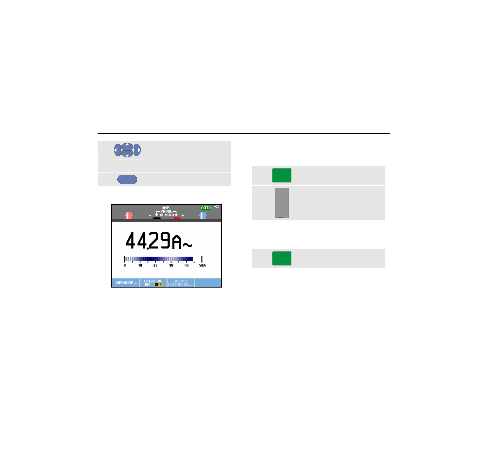
Fluke 190 Series II
Users Manual
6
Observe the sensitivity of the
current probe. Highlight the
corresponding sensitivity in the
menu, e.g. 1 mV/A.
7
ENTER
Accept the current measurement.
Now, you will see a screen like in Figure 17
Figure 17. Ampere Measurement Readings
Selecting Auto/Manual Ranges
To activate manual ranging, do the following during any
Meter measurement:
1
2
MANUAL
AUTO
mV
RANGE
V
Observe how the bargraph sensitivity changes.
Use manual ranging to set a fixed bargraph sensitivity and
decimal point.
3
MANUAL
AUTO
When in auto ranging, the bargraph sensitivity and decimal
point are automatically adjusted while checking different
signals.
Activate manual ranging.
Increase (V) or decrease (mV)
the range.
Choose auto ranging again.
38
Find Quality Products Online at: sales@GlobalTestSupply.com
www.GlobalTestSupply.com
Page 46

Using the Scope and Meter
Making Multimeter Measurements (for models 190-xx2)
1
Making Relative Meter Measurements
A relative measurement displays the present
measurement result relative to a defined reference value.
The following example shows how to perform a relative
voltage measurement. First obtain a reference value:
1
METER
Display the METER key labels.
2
3
F2
4
Measure a voltage to be used as
reference value.
Set RELATIVE to ON. (ON is
highlighted.) This stores the
reference value as reference for
subsequent measurements.
Observe the ADJUST REFERENCE
soft key (F3) that enables you to
adjust the reference value (see
step 5 below).
Measure the voltage to be
compared to the reference.
Now the large reading is the actual input value minus the
stored reference value. The bargraph indicates the actual
input value. The actual input value and the reference value
are displayed below the large reading (ACTUAL: xxxx
REFERENCE: xxx), see Figure 18.
Figure 18. Making a Relative Measurement
You can use this feature when, for example, you need to
monitor input activity (voltage, temperature) in relation to a
known good value.
39
Find Quality Products Online at: sales@GlobalTestSupply.com
www.GlobalTestSupply.com
Page 47

Fluke 190 Series II
Users Manual
Adjusting the reference value
To adjust the reference value, do the following:
5
6
7
8
40
F3
ENTER
Display the Adjust Reference
menu.
Select the digit you want to
adjust.
Adjust the digit. Repeat step 6
and step 7 until finished.
Enter the new reference value.
Find Quality Products Online at: sales@GlobalTestSupply.com
www.GlobalTestSupply.com
Page 48

About this Chapter
This chapter provides a step-by-step introduction to the
recorder functions of the test tool. The introduction gives
examples to show how to use the menus and perform
basic operations.
Opening the Recorder Main Menu
First choose a measurement in scope or meter mode. Now
you can choose the recorder functions from the recorder
main menu. To open the main menu, do the following:
Chapter 2
Using The Recorder Functions
1
RECORDER
Find Quality Products Online at: sales@GlobalTestSupply.com
Open the recorder main menu.
(See Figure 19).
www.GlobalTestSupply.com
Figure 19. Recorder Main Menu
Trendplot Meter is only present in models 190-xx2.
41
Page 49

Fluke 190 Series II
Users Manual
Plotting Measurements Over Time
(TrendPlot™)
Use the TrendPlot function to plot a graph of Scope or
Meter measurements (readings) as function of time.
Note
Because the navigations for the Trendplot Scope
and the Trendplot Meter are identical, only Scope
Trendplot is explained in the next sections.
Starting a TrendPlot Function
To start a TrendPlot, do the following:
1 Make automatic Scope or Meter measurements,
see Chapter 1. The readings will be plotted!
2
RECORDER
3 Highlight Trend Plot.
4
ENTER
The test tool continuously records the digital readings of
the measurements and displays these as a graph. The
TrendPlot graph rolls from right to left like a paper chart
recorder.
Observe that the recorded time from start appears at the
bottom of the screen. The present reading appears on top
of the screen. (See Figure 20.)
Open the RECORDER main menu.
Start the TrendPlot recording.
42
Find Quality Products Online at: sales@GlobalTestSupply.com
www.GlobalTestSupply.com
Page 50

Using The Recorder Functions
Plotting Measurements Over Time (TrendPlot™)
2
Note
When simultaneously TrendPlotting two readings,
the screen area is split into two sections of four
divisions each. When simultaneously
TrendPlotting three or four readings, the screen
area is split into three or four sections of two
divisions each.
Figure 20. TrendPlot Reading
When the test tool is in automatic mode, automatic vertical
scaling is used to fit the TrendPlot graph on the screen.
5
F1
6
F1
Scope TrendPlot is not possible on cursor related
measurements. As an alternative you may use
FlukeView logging of readings.
Set RECORDER to STOP to freeze
the recorder function.
Set RECORDER to RUN to restart.
Note
43
Find Quality Products Online at: sales@GlobalTestSupply.com
www.GlobalTestSupply.com
Page 51

Fluke 190 Series II
Users Manual
Displaying Recorded Data
When in normal view (NORMAL), only the twelve most
recently recorded divisions are displayed on screen. All
previous recordings are stored in memory.
VIEW ALL shows all data in memory:
7
F3
F3
Press
(NORMAL) and overview (VIEW ALL)
When the recorder memory is full, an automatic
compression algorithm is used to compress all samples
into half of the memory without loss of transients. The
other half of the recorder memory is free again to continue
recording.
Display an overview of the full
waveform.
repeatedly to toggle between normal view
Changing the Recorder Options
At the lower right of the display, the status line indicates a
time. You can choose this time to represent either the
start time of the recording (‘Time of Day’) or the time
elapsed since the start of the recording (‘From Start’).
To change the time reference, proceed from step 6 as
follows:
7
F2
Open the RECORDER OPTIONS
menu.
8
ENTER
Turning Off the TrendPlot Display
9
F4
Select Time of Day or From
Start
Exit the recorder function.
44
Find Quality Products Online at: sales@GlobalTestSupply.com
www.GlobalTestSupply.com
Page 52

Using The Recorder Functions
Recording Scope Waveforms In Deep Memory (Scope Record)
Recording Scope Waveforms In Deep
Memory (Scope Record)
The SCOPE RECORD function is a roll mode that logs a long
waveform of each active input. This function can be used
to monitor waveforms like motion control signals or the
power-on event of an Uninterruptable Power Supply
(UPS). During recording, fast transients are captured.
Because of the deep memory, recording can be done for
more than one day. This function is similar to the roll mode
in many DSO’s but has deeper memory and better
functionality.
Starting a Scope Record Function
To record for example the input A and input B waveform,
do the following:
1 Apply a signal to input A and input B.
2
RECORDER
Open the RECORDER main menu.
Observe that the screen displays the following:
• Time from start at the top of the screen.
• The status at the bottom of the screen which includes
Figure 21. Recording Waveforms
the time/div setting as well as the total timespan that
fits the memory.
2
3
ENTER
The waveform moves across the screen from right to left
like on a normal chart recorder. (See Figure 21).
From the Recorder main menu,
highlight Scope Record and Start
the recording.
Note
For accurate recordings it is advised to let the
instrument first warm up for five minutes.
45
Find Quality Products Online at: sales@GlobalTestSupply.com
www.GlobalTestSupply.com
Page 53

Fluke 190 Series II
Users Manual
Displaying Recorded Data
In Normal view, the samples that roll off the screen are
stored in deep memory. When the memory is full,
recording continues by shifting the data in memory and
deleting the first samples out of memory.
In View All mode, the complete memory contents are
displayed on the screen.
4
F3
You can analyze the recorded waveforms using the
Cursors and Zoom functions. See Chapter 3: “Using
Replay, Zoom and Cursors”.
Press to toggle between VIEW ALL
(overview of all recorded
samples) and NORMAL view.
Using Scope Record in Single Sweep Mode
Use the recorder Single Sweep function to automatically
stop recording when the deep memory is full.
Continue from step 3 of the previous section:
4
F1
5
F2
6
ENTER
7
F1
Stop recording to unlock the
OPTIONS… softkey
Open the RECORDER OPTIONS
menu.
Jump to the Mode field, select
Single Sweep and accept the
recorder options.
Start recording.
46
Find Quality Products Online at: sales@GlobalTestSupply.com
www.GlobalTestSupply.com
Page 54

Using The Recorder Functions
Recording Scope Waveforms In Deep Memory (Scope Record)
2
Using Triggering to Start or Stop Scope Record
To record an electrical event that causes a fault, it might
be useful to start or stop recording on a trigger signal:
Start on trigger to start recording; recording stops when
the deep memory is full
Stop on trigger to stop recording.
Stop when untriggered to continue recording as long as
a next trigger comes within 1 division in view all mode.
For the models 190-xx4 the signal on the BNC input that
has been selected as trigger source must cause the
trigger.
For the models 190-xx2 the signal applied to the banana
jack inputs (
trigger. The trigger source is automatically set to Ext.
(external).
To set up the test tool, continue from step 3 of the
previous section:
4 Apply the signal to be recorded to the BNC
5
EXT TRIGGER (in)). signal must cause the
input(s).
F1
Stop recording to unlock the
OPTIONS… softkey
6
F2
7
ENTER
8
ENTER
For external triggering (190-xx2) continue at step 9.
Open the RECORDER OPTIONS
menu.
Jump to the Mode: field, select
on Trigger… (models 190-xx4) or
on Ext. (models 190-xx2) to open
the START SINGLE SWEEP ON
TRIGGERING or the START SINGLE
SWEEP ON EXT. menu.
Select one of the Conditions:
and accept the selection.
47
Find Quality Products Online at: sales@GlobalTestSupply.com
www.GlobalTestSupply.com
Page 55

Fluke 190 Series II
Users Manual
9
ENTER
10
ENTER
11 Apply a trigger signal to the red and black ext.
trigger banana inputs.
During recording samples are continuously saved in deep
memory. The last twelve recorded divisions are displayed
on the screen. Use View All to display the full memory
contents.
To learn more about the Single Shot trigger
function, see Chapter 4 “Triggering on
Waveforms”.
Select the desired trigger slope
(Slope:) and jump to Level:
Select the 0.12V or 1.2V trigger
level and accept all recorder
options.
Note
Figure 22. Triggered Single Sweep Recording
Analyzing a TrendPlot or Scope Record
From a TrendPlot or Scope Record you can use the
analysis functions CURSORS and ZOOM to perform
detailed waveform analysis. These functions are described
in Chapter 3: “Using Replay, Zoom and Cursors”.
48
Find Quality Products Online at: sales@GlobalTestSupply.com
www.GlobalTestSupply.com
Page 56

Using Replay, Zoom and Cursors
About this Chapter
This chapter covers the capabilities of the analysis
functions Cursor, Zoom, and Replay. These functions
can be used with one or more of the primary functions
Scope, TrendPlot or Scope Record.
It is possible to combine two or three analysis functions. A
typical application using these functions follows:
• First replay the last screens to find the screen of
special interest.
• Then zoom in on the signal event.
• Finally, make measurements using the cursors.
Chapter 3
Replaying the 100 Most Recent Scope
Screens
When you are in scope mode, the test tool automatically
stores the 100 most recent screens. When you press the
HOLD key or the REPLAY key, the memory contents are
frozen. Use the functions in the REPLAY menu to “go back
in time” by stepping through the stored screens to find the
screen of your interest. This feature lets you capture and
view signals even if you did not press
HOLD.
49
Find Quality Products Online at: sales@GlobalTestSupply.com
www.GlobalTestSupply.com
Page 57

Fluke 190 Series II
Users Manual
Replaying Step-by-Step
To step through the last scope screens, do the following:
1
REPLAY
From scope mode, open the
REPLAY menu.
Observe that the trace is frozen
and that REPLAY appears at the
top of the screen (see Figure 23).
2
F1
3
F2
Observe that the bottom of the waveform area displays the
replay bar with a screen number and related time stamp:
Step through the previous
screens.
Step through the next screens.
50
Figure 23. Replaying a Waveform
The replay bar represents all 100 stored screens in
memory. The icon represents the picture being
displayed on the screen (in this example: SCREEN -51). If
the bar is partly white, the memory is not completely filled
with 100 screens.
From this point you can use the zoom and cursor functions
to study the signal in more detail.
Find Quality Products Online at: sales@GlobalTestSupply.com
www.GlobalTestSupply.com
Page 58

Using Replay, Zoom and Cursors
Replaying the 100 Most Recent Scope Screens
3
Replaying Continuously
You can also replay the stored screens continuously, like
playing a video tape.
To replay continuously, do the following:
1
2
Wait until the screen with the signal event of interest
appears.
3
REPLAY
F3
F3
From Scope mode, open the
REPLAY menu.
Observe that the trace is frozen
and REPLAY appears at the top of
the screen.
Continuously replay the stored
screens in ascending order.
Stop the continuous replay.
Turning Off the Replay Function
4
F4
Turn off REPLAY.
Capturing 100 Intermittents Automatically
When you use the test tool in triggered mode, 100
triggered screens are captured.
By combining the trigger possibilities with the capability of
capturing 100 screens for later replay, you can leave the
test tool unattended to capture intermittent signal
anomalies. This way you could use Pulse Triggering to
trigger and capture 100 intermittent glitches or you could
capture 100 UPS startups.
For triggering, see Chapter 4: “Triggering on Waveforms”.
51
Find Quality Products Online at: sales@GlobalTestSupply.com
www.GlobalTestSupply.com
Page 59

Fluke 190 Series II
Users Manual
Zooming in on a Waveform
To obtain a more detailed view of a waveform, you can
zoom in on a waveform using the
To zoom in on a waveform, do the following:
ZOOM function.
1
ZOOM
Display the ZOOM key labels.
ZOOM appears at the top of the
screen, and the waveform is
magnified.
2
3
Enlarge (decrease the time/div) or
shrink (increase the time/div) the
waveform.
Scroll. A position bar displays the
position of the zoomed part in
relation to the total waveform.
Tip
Even when the key labels are not displayed at the
bottom of the screen, you can still use the arrow
keys to zoom in and out. You can also use the
TIME ns
52
key to zoom in and out.
Figure 24. Zooming in a Waveform
Observe that the bottom of the waveform area displays the
zoom ratio, position bar, and time/div (see Figure 24). The
zoom range depends on the amount of data samples
stored in memory.
Turning Off the Zoom Function
4
F4
s
Turn off the ZOOM function.
Find Quality Products Online at: sales@GlobalTestSupply.com
www.GlobalTestSupply.com
Page 60

Using Replay, Zoom and Cursors
Making Cursor Measurements
3
Making Cursor Measurements
Cursors allow you to make precise digital measurements
on waveforms. This can be done on live waveforms,
recorded waveforms, and on saved waveforms.
Using Horizontal Cursors on a Waveform
To use the cursors for a voltage measurement, do the
following:
1
CURSOR
2
F1
3
F2
4
5
F2
6
From scope mode, display the
cursor key labels.
Press to highlight . Observe
that two horizontal cursors are
displayed.
Highlight the upper cursor.
Move the upper cursor to the
desired position on the screen.
Highlight the lower cursor.
Move the lower cursor to the
desired position on the screen.
Note
Even when the key labels are not displayed at the
bottom of the screen, you still can use the arrow
keys. This allows full control of both cursors while
having full screen view.
Figure 25. Voltage Measurement with Cursors
The screen shows the voltage difference between the two
cursors and the voltage at the cursors. (See Figure 25.)
Use horizontal cursors to measure the amplitude, high or
low value, or overshoot of a waveform.
53
Find Quality Products Online at: sales@GlobalTestSupply.com
www.GlobalTestSupply.com
Page 61

Fluke 190 Series II
Users Manual
Using Vertical Cursors on a Waveform
To use the cursors for a time measurement (T, 1/T), for a
mVs-mAs-mWs measurement, or for an RMS
measurement of the trace section between the cursors, do
the following:
1
CURSOR
From scope mode, display the
cursor key labels.
2
F1
3
F3
4
F4
5
F2
6
Press to highlight . Observe
that two vertical cursors are
displayed. Markers (—) identify the
selected point where the cursors
cross the waveform.
Choose, for example, time
measurement: T.
Choose the trace that you want
the markers to be placed on:
A ,B, C, D or M (Mathematics).
Highlight the left cursor.
Move the left cursor to the desired
position on the waveform.
7
F2
Highlight the right cursor.
Figure 26. Time Measurement with Cursors
8
The screen shows the time difference between the cursors
and the voltage difference between the two markers. (See
Figure 26.)
9
F4
Move the right cursor to the
desired position on the waveform.
Select OFF to turn off the cursors.
54
Find Quality Products Online at: sales@GlobalTestSupply.com
www.GlobalTestSupply.com
Page 62

Using Replay, Zoom and Cursors
Making Cursor Measurements
3
Notes
− For mVs select probe type ‘Voltage’.
− For mAs select probe type ‘Current’.
− For mWs select mathematical function x,
and probe type ‘Voltage’ for one channel
and ‘Current’ for the other channel.
Using Cursors on a Mathematical Result (+ - x)
Waveform
Cursor measurements on, for examle, a AxB waveform
give a reading in Watts if input A measures (milli)Volts and
input B measures (milli)Amperes.
For other cursor measurements on, for example, a A+B,
A-B or AxB waveform no reading will be available if the
input A and input B measurement unit are different.
Using Cursors on Spectrum Measurements
To do a cursor measurent on a spectrum, do the following:
1
CURSOR
From Spectrum measurement
display the cursor key label.
2
Move the cursor and observe the
readings at the top of the screen.
55
Find Quality Products Online at: sales@GlobalTestSupply.com
www.GlobalTestSupply.com
Page 63

Fluke 190 Series II
Users Manual
Making Rise Time Measurements
To measure rise time, do the following:
1
2
3
4
5
6
7
CURSOR
F1
F4
F3
F2
From scope mode, display the
cursor key labels.
Press to highlight (rise time).
Observe that two horizontal
cursors are displayed.
For multiple traces select the
required trace A, B, C, D or M (if a
math function is active).
Select MANUAL or AUTO (this
automatically does steps 5 to 7).
Move the upper cursor to 100% of
the trace height. A marker is
shown at 90%.
Highlight the other cursor.
Move the lower cursor to 0% of
the trace height. A marker is
shown at 10%.
The reading shows the risetime from 10%-90% of the
trace amplitude.
Figure 27. Risetime Measurement
56
Find Quality Products Online at: sales@GlobalTestSupply.com
www.GlobalTestSupply.com
Page 64

About this Chapter
This chapter provides an introduction to the trigger
functions of the test tool. Triggering tells the test tool when
to begin displaying the waveform. You can use fully
automatic triggering, take control of one or more main
trigger functions (semi-automatic triggering), or you can
use dedicated trigger functions to capture special
waveforms.
Following are some typical trigger applications:
• Use the Connect-and-View™ function to have full
automatic triggering and instant display of virtually any
waveform.
Chapter 4
Triggering on Waveforms
• If the signal is unstable or has a very low frequency,
you can control the trigger level, slope, and trigger
delay for a better view of the signal. (See next
section.)
• For dedicated applications, use one of the three
manual trigger functions:
• Edge triggering
• Video triggering
• Pulse Width triggering
• External Triggering (models 190-xx2 only)
57
Find Quality Products Online at: sales@GlobalTestSupply.com
www.GlobalTestSupply.com
Page 65

Fluke 190 series II
Users Manual
Setting Trigger Level and Slope
The Connect-and-View™ function enables hands-off
triggering to display complex unknown signals.
When your test tool is in manual range, do the following:
Automatic triggering assures a stable display of virtually
any signal.
From this point, you can take over the basic trigger
controls such as level, slope and delay. To optimize trigger
level and slope manually, do the following:
1
MANUAL
AUTO
TRIGGER
Perform an auto set. AUTO appears
at the top right of the screen.
Display the TRIGGER key labels.
2
3
58
F2
F3
Trigger on either positive slope or
negative slope of the chosen
waveform.
In Dual Slope Triggering ( X ) the
test tool triggers on both positive
slope and negative slope.
Enable the arrow keys for manual
trigger level adjustment.
Figure 28. Screen with all Trigger Information
4 Adjust the trigger level.
Observe the trigger icon that indicates the trigger
position, trigger level, and slope.
At the bottom of the screen the trigger parameters are
displayed (See Figure 28). For example,
means that input A is used as the trigger source with a
positive slope.
When a valid trigger signal is found, the trigger key will be
lit and the trigger parameters appear in black.
When no trigger is found, the trigger parameters appear in
gray, ands the key light will be off.
Find Quality Products Online at: sales@GlobalTestSupply.com
www.GlobalTestSupply.com
Page 66

Triggering on Waveforms
Using Trigger Delay or Pre-trigger
4
Using Trigger Delay or Pre-trigger
You can begin to display the waveform some time before
or after the trigger point has been detected. Initially, you
have a half screen (6 divisions) of pre-trigger view
(negative delay).
To set the trigger delay, do the following:
5
Observe that the trigger icon on the screen moves to
show the new trigger position. When the trigger position
moves left off of the screen, the trigger icon changes into
Moving the trigger icon to the right on the display gives
you a pre-trigger view. This allows you to see what
happened before the trigger event, or what caused the
trigger.
In case of a trigger delay, the status at the bottom of the
screen will change. For example:
This means that input A is used as the trigger source with
a positive slope. The 500.0 ms indicates the (positive)
delay between trigger point and waveform display.
MOVE
to indicate that you have selected a trigger delay.
Hold down to adjust the trigger
delay.
When a valid trigger signal is found, the trigger key will be
lit and the trigger parameters appear in black.
When no trigger is found, the trigger parameters appear in
gray, ands the key light will be off.
Figure 29. Trigger Delay or Pre-trigger View
Figure 29 shows an example of a trigger delay of 500 ms
(top) and an example of pre-trigger view of 8 divisions
(bottom).
59
Find Quality Products Online at: sales@GlobalTestSupply.com
www.GlobalTestSupply.com
Page 67

Fluke 190 series II
Users Manual
Automatic Trigger Options
In the trigger menu, settings for automatic triggering can
be changed as follows. (See also Chapter 1: “Displaying
an Unknown Signal with Connect-and-View”)
1
TRIGGER
The
TRIGGER key labels can differ depending on
the latest trigger function used.
2
F4
3
ENTER
Display the TRIGGER key labels.
Note
Open the TRIGGER OPTIONS menu.
Open the AUTOMATIC TRIGGER menu.
If the frequency range of the automatic triggering is set to
> 15 Hz, the Connect-and-View™ function responds more
quickly. The response is quicker because the test tool is
instructed not to analyze low frequency signal
components. However, when you measure frequencies
lower than 15 Hz, the test tool must be instructed to
analyze low frequency components for automatic
triggering:
4
ENTER
Select > 1 HZ and return to the
measurement screen.
60
Find Quality Products Online at: sales@GlobalTestSupply.com
www.GlobalTestSupply.com
Page 68

Triggering on Waveforms
Triggering on Edges
4
Triggering on Edges
If the signal is unstable or has a very low frequency, use
edge triggering to obtain full manual trigger control.
To trigger on rising edges of the input A waveform, do the
following:
1
TRIGGER
2
F4
3
ENTER
Display the TRIGGER key labels.
Open the TRIGGER OPTIONS menu.
Open the TRIGGER ON EDGE menu.
When Free Run is selected, the test tool updates the
screen even if there are no triggers. A trace always
appears on the screen.
When On Trigger is selected, the test tool needs a trigger
to display a waveform. Use this mode if you want to
update the screen only when valid triggers occur.
When Single Shot is selected, the test tool waits for a
trigger. After receiving a trigger, the waveform is displayed
and the instrument is set to HOLD.
In most cases it is advised to use the Free Run mode:
4
ENTER
5
ENTER
Observe that the key labels at the bottom of the screen
have adapted to allow further selection of specific edge
trigger settings:
Select Free Run, jump to Trigger
Filter.
Set Trigger Filter to Off.
61
Find Quality Products Online at: sales@GlobalTestSupply.com
www.GlobalTestSupply.com
Page 69

Fluke 190 series II
Users Manual
Triggering on Noisy Waveforms
To reduce jitter on the screen when triggering on noisy
waveforms, you can use a trigger filter. Continue from step
3 of the previous example as follows:
4
ENTER
5
ENTER
When Noise Reject is on, an increased trigger gap will be
applied.
When HF Reject is on, HF noise on the (internal) trigger
signal will be suppressed.
Select On Trigger, jump to Trigger
Filter.
Set Noise Reject or HF Reject to
On. This is indicated by a taller
trigger icon .
Making a Single Acquisition
To catch single events, you can perform a single shot
acquisition (one-time screen update). To set up the test
tool for a single shot of the input A waveform, continue
from step 3 (page 61) again:
4
ENTER
Select Single Shot.
The word
indicating that the test tool is waiting for a trigger. As soon
as the test tool receives a trigger, the waveform is
displayed and the instrument is set to hold. This is
indicated by the word HOLD at top of the screen.
The test tool will now have a screen like Figure 30.
5
MANUAL appears at the top of the screen
HOLD
RUN
Arm the test tool for a new single
shot.
Tip
The test tool stores all single shots in the replay
memory. Use the Replay function to look at all
the stored single shots (see Chapter 3).
Figure 30. Making a Single Shot Measurement
62
Find Quality Products Online at: sales@GlobalTestSupply.com
www.GlobalTestSupply.com
Page 70

Triggering on Waveforms
Triggering on Edges
4
N-Cycle Triggering
N-Cycle triggering enables you to create a stable picture of
for example n-cycle burst waveforms.
Each next trigger is generated after the waveform has
crossed the trigger level N times in the direction that
complies with the selected trigger slope.
To select N-Cycle triggering, continue from step 3 (page
61) again:
4
ENTER
5
ENTER
6
ENTER
Observe that the key labels at the bottom of the screen
have been changed to allow further selection of specific
N-Cycle trigger settings:
Select On Trigger or Single Shot,
jump to Trigger Filter.
Select a Trigger Filter or set it Off.
Set NCycle to On
7
Set the number of cycles N
8 Adjust the trigger level
Traces with N-Cycle triggering (N=2) and without N-Cycle
triggering are shown in Figure 31.
Figure 31. N-Cycle triggering
63
Find Quality Products Online at: sales@GlobalTestSupply.com
www.GlobalTestSupply.com
Page 71

Fluke 190 series II
Users Manual
Triggering on External Waveforms
(models 190-xx2)
Use external triggering when you want to display
waveforms on inputs A and B while triggering on a third
signal. You can choose external triggering with automatic
triggering or with edge triggering.
1 Supply a signal to the red and black 4-mm
banana jack inputs.
In this example you continue from the Trigger on Edges
example. To choose the external signal as trigger source,
continue as follows:
2
TRIGGER
3
F1
Display the TRIGGER (On Edges)
key labels.
Select Ext (external) edge trigger.
Observe that the key labels at the bottom of the screen
have been adapted to allow selection of two different
external trigger levels: 0.12 V and 1.2 V:
4
F3
From this point the trigger level is fixed and is compatible
with logic signals.
Select 1.2V under the Ext LEVEL
label.
64
Find Quality Products Online at: sales@GlobalTestSupply.com
www.GlobalTestSupply.com
Page 72

Triggering on Waveforms
Triggering on Video Signals
Triggering on Video Signals
To trigger on a video signal, first select the standard of the
video signal you are going to measure:
1 Apply a video signal to the red input A.
4
2
TRIGGER
Display the TRIGGER key labels.
3
F4
Open the Trigger Options menu.
Figure 32. Measuring Interlaced Video Signals
4
ENTER
5
ENTER
Select Video on A … to open the
TRIGGER ON VIDEO menu.
Select positive signal polarity for
video signals with negative going
sync pulses.
6
ENTER
Trigger level and slope are now fixed.
Observe that the key labels at the bottom of the screen
have been changed to allow further selection of specific
video trigger settings.
65
Select a video standard or Non
interlaced… and return.
If you select Non interlaced a
scan rate selection menu will
open.
Find Quality Products Online at: sales@GlobalTestSupply.com
www.GlobalTestSupply.com
Page 73

Fluke 190 series II
Users Manual
Triggering on Video Frames
Use FIELD 1 or FIELD 2 to trigger either on the first half of
the frame (odd) or on the second half of the frame
(even).To trigger on the second half of the frame, do the
following:
7
F1
The signal part of the even field is displayed on the
screen.
Choose FIELD 2.
Triggering on Video Lines
Use ALL LINES to trigger on all line synchronization
pulses (horizontal synchronization).
7
F2
The signal of one line is displayed on the screen. The
screen is updated with the signal of the next line
immediately after the test tool triggers on the horizontal
synchronization pulse.
To view a specific video line in more detail, you can select
the line number. For example, to measure on video line
123, continue from step 6 as follows:
7
F3
8 Select number 123.
The signal of line 123 is displayed on the screen. Observe
that the status line now also shows the selected line
number. The screen is continuously updated with the
signal of line 123.
Choose ALL LINES.
Enable video line selection.
66
Find Quality Products Online at: sales@GlobalTestSupply.com
www.GlobalTestSupply.com
Page 74

Triggering on Waveforms
Triggering on Pulses
4
Triggering on Pulses
Use pulse width triggering to isolate and display specific
pulses that you can qualify by time, such as glitches,
missing pulses, bursts or signal dropouts.
Detecting Narrow Pulses
To set the test tool to trigger on narrow positive pulses
shorter than 5 ms, do the following:
1 Apply a video signal to the red input A.
2
TRIGGER
3
F4
4
ENTER
Display the TRIGGER key labels.
Open the TRIGGER OPTIONS menu.
Select Pulse Width on A... to open
the trigger on pulse width menu.
5
ENTER
6
ENTER
7
ENTER
The test tool is now prepared to trigger on narrow pulses
only. Observe that the trigger key labels at the bottom of
the screen have been adapted to set the pulse conditions:
Select the positive pulse icon,
then jump to Condition.
Select <t, then jump to Update.
Select On Trigger.
To set the pulse width to 5 ms, do the following:
8
F1
9 Select 5 ms.
All narrow positive pulses shorter than 5 ms are now
displayed on the screen. (See Figure 33).
Enable the arrow keys to adjust
the pulse width.
67
Find Quality Products Online at: sales@GlobalTestSupply.com
www.GlobalTestSupply.com
Page 75

Fluke 190 series II
Users Manual
Tip
The test tool stores all triggered screens in the
replay memory. For example, if you setup your
triggering for glitches, you can capture 100
glitches with time stamps. Use the REPLAY key to
look at all the stored glitches.
Figure 33. Triggering on Narrow Glitches
Finding Missing Pulses
The next example covers finding missing pulses in a train
of positive pulses. In this example it is assumed that the
pulses have a 100 ms distance between the rising edges.
If the time accidently increases to 200 ms, a pulse is
missing. To set the test tool to trigger on such missing
pulses, let it trigger on gaps bigger than about 110 ms.
Do the following:
1
TRIGGER
Display the TRIGGER key labels.
2
F4
Open the TRIGGER OPTIONS menu.
3
ENTER
Select Pulse Width on A... to
open the TRIGGER ON PULSE WIDTH
menu.
68
Find Quality Products Online at: sales@GlobalTestSupply.com
www.GlobalTestSupply.com
Page 76

Triggering on Waveforms
Triggering on Pulses
4
4
ENTER
5
ENTER
6
ENTER
The test tool is now prepared to trigger on pulses that are
more than a selectable time in duration. Observe that the
trigger menu at the bottom of the screen has been
adapted to set the pulse condition:
Select the positive pulse icon to
trigger on a positive pulse, then
jump to Condition:
Select >t, then jump to Update:
Select On Trigger and exit the
menu.
To set the pulse width to 110 ms, continue as follows:
7
F1
8
Enable the arrow keys to adjust
the pulse width.
Select 110 ms.
Figure 34. Triggering on Missing Pulses
69
Find Quality Products Online at: sales@GlobalTestSupply.com
www.GlobalTestSupply.com
Page 77

About this Chapter
This chapter provides a step-by-step introduction to the
general functions of the test tool that can be used in the
three main modes: Scope, Meter, or Recorder. You will
find information on computer communication at the end of
this chapter.
Chapter 5
Using Memory and PC
The ports are fully isolated from the input channels and
are covered with dust covers when not in use.
Using the USB Ports
The test tool is provided with two USB ports:
• a USB-host port to connect an external flash memory
drive (‘USB-stick’) for data storage.
• a mini-USB-B port which allows you to connect the
test tool to a PC for remote control and data transfer
under PC-control, see Using FlukeView
®
on page 80.
USB stick
Mini USB
Figure 35. Test Tool USB Connections
71
Find Quality Products Online at: sales@GlobalTestSupply.com
www.GlobalTestSupply.com
Page 78

Fluke 190 series II
Users Manual
Saving and Recalling
You can:
• Save screens and setups to internal memory, and
recall them again from memory. The test tool has 15
‘screen and setup’ memories, 2 ‘record and setup’
memories, and 1 screen image memory. See also
Table 1.
• Save up to 256 screens and setups to a USB memory
device, and recall them again from memory.
• Name saved screens and setups according to your
own preferences.
• Recall screens and recordings to analyze the screen
image at a later date.
• Recall a setup to continue a measurement with the
recalled operating configuration.
Notes
Saved data are stored in non-volatile Flash
memory.
Not saved instrument data are stored in RAM
memory and will be kept at least 30 seconds
when the battery is removed when no power is
supplied via the BC190 power adapter.
Table 1. Test Tool Internal Memory
Mode Memory locations
30x 10x 9x
METER Setup +
1 screen
SCOPE Setup +
1 screen
SCOPE REC - Setup +
TRENDPLOT - Setup +
Setup +
100 replay
screens
record data
trendplot data
- Screen image
Screen image
Screen image
Screen image
In persistence mode the most recently written trace will be
saved, not all persistence traces.
In the displayed file list of stored screens and setups the
following symbols are used:
setup + 1 screen
setup + replay screens/record data
setup + trendplot data
screen image (imagexxx.bmp)
72
Find Quality Products Online at: sales@GlobalTestSupply.com
www.GlobalTestSupply.com
Page 79

Using Memory and PC
Saving and Recalling
5
Saving Screens with Associated Setups
To save for example a screen+setup in Scope mode, do
the following:
1
SAVE
Display the SAVE key labels.
From this point the screen is frozen.
2
F1
Open the SAVE menu.
Observe the number of available
and used memory locations.
In METER mode the SAVE AS menu
will be shown now as only a
setup+screen can be saved, see
step 4.
3
F1
4
ENTER
Select the target memory INT
(internal memory) or USB (USB
device).
Observe the new SAVE menu if you
select USB.
Select Screen+Setup and open
the SAVE AS menu.
5
To resume your measurements press
ENTER
Below Save As: the default name +
serial number and OK SAVE are
already selected.
To modify the name for this
particular Screen+Setup or to
modify the default name see below
‘Editing Names’.
Save the Screen+setup.
HOLD
.
RUN
73
Find Quality Products Online at: sales@GlobalTestSupply.com
www.GlobalTestSupply.com
Page 80

Fluke 190 series II
Users Manual
All memories in use
If no free memory locations are available a message pops
up that proposes to you to overwrite the oldest data set.
Do one of the following:
If you don’t want to overwrite the oldest data set,
- press
F3
, then delete one or more memory
locations, and save again.
If you want to overwrite the oldest data set,
- press
F4
.
Editing names
To name the screen+setup according to your own
preferences, continue from step 4 as follows:
5
F1
6
F2
F3
7
ENTER
Open the EDIT NAME menu
Skip to a new character position.
Select another character and press
ENTER to accept your choice.
Repeat 6 and 7 until done.
8
F1
9
ENTER
Accept the name and return to the
SAVE AS menu.
Highlight OK SAVE to save the
actual screen using the edited
name.
To modify the default name generated by the test tool,
continue from step 8 as follows:
9
ENTER
Highlight SET DEFAULT to save
the new default name
74
Find Quality Products Online at: sales@GlobalTestSupply.com
www.GlobalTestSupply.com
Page 81

Using Memory and PC
Saving and Recalling
5
10
ENTER
The ‘record+setup’ memory locations store more than just
what is visible on the screen. In TrendPlot or Scope
Record mode the full recording is saved. In scope mode
you can save all 100 replay screens in a single
record+setup memory location. The table below shows
what you can store for the various test tool modes.
To save a TrendPlot press STOP first.
Highlight OK SAVE to save the
actual screen using the new default
name.
Notes
Saving Screens in .bmp Format (Print Screen)
To save a screen in bitmap (.bmp) format, do the
following:
1
SAVE
Display the SAVE key labels.
2
F3
The file is saved using a fixed name (IMAGE) and a serial
number, for example IMAGE004.bmp.
If no free memory locations are available a message pops
up that proposes to you to overwrite the oldest data set.
Do one of the following:
If you don’t want to overwrite the oldest data set,
- press
If you want to overwrite the oldest data set,
F3
locations, and save again.
Save the screen to:
− Internal memory (INT) if no
USB device is connected
− a USB device if connected.
, then delete one or more memory
- press
F4
.
75
Find Quality Products Online at: sales@GlobalTestSupply.com
www.GlobalTestSupply.com
Page 82

Fluke 190 series II
Users Manual
Deleting Screens with Associated Setups
To delete a screen and associated setup, do the following:
1
SAVE
Display the SAVE key labels.
2
F4
3
F1
4
5
6
ENTER
F2
7
ENTER
Open the FILE OPTIONS menu.
Select the source, internal memory
(INT) or a USB device.
Highlight DELETE ,
Accept your choice and jump to the
filename field
Select the file to be deleted,
Or
Select all files for deletion
Delete the selected files.
Recalling Screens with Associated Setups
To recall a screen+setup, do the following:
1
SAVE
2
F2
3
F1
4
5
6
7
Observe that the recalled waveform is displayed and that
HOLD appears on the screen. From this point you can use
cursors and zoom for analysis or you can print the recalled
screen.
To recall a screen as a reference waveform to compare it
to an actually measured waveform, see Chapter 1
‘Comparing Waveforms’.
ENTER
ENTER
Display the SAVE key labels.
Open the RECALL menu.
Select the source, internal memory
(INT) or a USB device.
Highlight DATA.
Accept your choice and jump to the
filename field
Select the file to be recalled,
Recall the selected screen+setup.
76
Find Quality Products Online at: sales@GlobalTestSupply.com
www.GlobalTestSupply.com
Page 83

Using Memory and PC
Saving and Recalling
5
Recalling a Setup Configuration
To recall a setup configuration, do the following:
1
SAVE
Display the SAVE key labels.
2
F2
3
F1
4
5
6
7
From this point you continue in the new operating
configuration.
ENTER
ENTER
Open the RECALL menu.
Select the source, internal memory
(INT) or a USB device.
Highlight SETUP.
Accept your choice and jump to the
filename field.
Select the file to be recalled,
Recall the selected setup.
Viewing Stored Screens
To scroll through the memories while looking at the stored
screens, do the following:
1
2
3
4
5
6
SAVE
F2
F1
ENTER
F2
Display the SAVE key labels.
Open the RECALL menu.
Select the source, internal memory
(INT) or a USB device.
Jump to the filename field.
Highlight a file .
View the screen, and open the
viewer.
7
8
F3
Scroll through all stored screens.
Print screen, saves the screen to
USB device (if connected) or
internal memory.
77
Find Quality Products Online at: sales@GlobalTestSupply.com
www.GlobalTestSupply.com
Page 84

Fluke 190 series II
Users Manual
9
F4
In the VIEW mode the replay screens of a saved
‘record+setup’ cannot be viewed! Only the screen
at the instant of saving can be reviewed in this
way. To see all replay screens recall them from
memory using the RECALL option.
Exit the View mode.
Note:
Renaming Stored Screens and Setup Files
To modify the name of stored files, do the following:
1
SAVE
Display the SAVE key labels.
2
F4
3
F1
4
5
ENTER
Open the FILE OPTIONS menu.
Select the source, internal memory
(INT) or a USB device.
Highlight RENAME.
Accept your choice and jump to the
filename field.
6
7
8
9
10
ENTER
F2
F3
ENTER
F1
Highlight the file to be renamed.
Open the RENAME menu.
Skip to a new character position.
Select another character.
Repeat 8 and 9 until done.
Accept the name and return to the
RENAME menu.
78
Find Quality Products Online at: sales@GlobalTestSupply.com
www.GlobalTestSupply.com
Page 85

Using Memory and PC
Saving and Recalling
5
Copying-Moving Stored Screens and Setup Files
You can copy or move a file from internal memory to a
USB device or from a USB device to internal memory.
To copy or to move a file, do the following:
1
SAVE
Display the SAVE key labels.
2
F4
3
F1
4
5
ENTER
Open the FILE OPTIONS menu.
Select the source, internal memory
(INT) or a USB device. The other
memory will become the
destination.
Highlight COPY to copy or MOVE to
move (copy and delete source) a
file.
Accept your choice and jump to the
filename field.
6
F2
7
ENTER
Select the file to be copied or
moved,
Or
Select all files
Copy or delete the selected files.
79
Find Quality Products Online at: sales@GlobalTestSupply.com
www.GlobalTestSupply.com
Page 86

Fluke 190 series II
Users Manual
Using FlukeView®
With the FlukeView® software you can upload waveform
data and screen bitmaps to your PC or notebook computer
for further processing.
USB drivers for the test tool and a FlukeView
version with restricted functionality are available on the
CD-ROM included in the shipment.
Connecting to a Computer
To connect the test tool to a PC or notebook computer and
use the FlukeView software for Windows® (SW90W), do
the following:
z Use a USB-A to mini-USB-B interface cable to
connect a computer to the mini USB PORT of the test
tool (See Figure 36).
z Install the test tool USB drivers, see Appendix A.
z Install the FlukeView
about installing and using the FlukeView
ScopeMeter software see the FlukeView
Manual on the CD ROM.
®
Demo version. For information
®
Demo
®
®
Users
Figure 36. Connecting a Computer
Notes
− The optional kit SCC290 contains an
activation code to convert the FlukeView
®
Demo version into a fully operational version.
− A complete FlukeView
®
version can be
ordered using ordering code SW90W. For
use with the Fluke Series II ScopeMeter test
tools FlukeView® ScopeMeter release V5.0
or higher is required.
− The test tool input channels are electrically
isolated from the USB port.
− Remote control and data transfer via mini-
USB is not possible while saving or recalling
data to or from the USB-stick..
80
Find Quality Products Online at: sales@GlobalTestSupply.com
www.GlobalTestSupply.com
Page 87

About this Chapter
This chapter gives you information and tips on how you
can make the best use of the test tool.
Chapter 6
Tips
Using the Standard Accessories
The following illustrations show the use of the standard
accessories such as voltage probes, test leads, and the
various clips.
81
Find Quality Products Online at: sales@GlobalTestSupply.com
www.GlobalTestSupply.com
Page 88

Fluke 190 Series II
Users Manual
A
Figure 37. HF Voltage Probe Connection Using
Ground Spring
Warning
To avoid electrical shock or fire, do not
connect the ground spring to voltages higher
than 30 Vrms from earth ground.
Figure 38. HF Voltage Probe Connection Using Probe
Tip to BNC Adapter (190-5xx)
Warning
To avoid electrical shock or fire, do not
connect the probe tip to BNC adapter to
voltages higher than 30 Vrms from earth
ground.
82
Find Quality Products Online at: sales@GlobalTestSupply.com
www.GlobalTestSupply.com
Page 89

Tips
Using the Independently Floating Isolated Inputs
Using the Independently Floating
Isolated Inputs
You can use the independently floating isolated inputs to
measure signals that are independently floating from each
other.
Independently floating isolated inputs offer additional
safety and measurement capabilities compared to inputs
with common references or grounds.
Measuring Using Independently Floating Isolated
Inputs
The test tool has independently floating isolated inputs.
Each input section (A, B, C, D – A, B, METER INPUT) has
its own signal input and its own reference input. The
reference input of each input section is electrically isolated
from the reference inputs of the other input sections. The
isolated input architecture makes the test tool about as
versatile as having four independent instruments. The
advantages of having independently floating isolated
inputs are:
• It allows simultaneous measurement of independently
floating signals.
Figure 39. Electronic Connections for Measurements
Using Hook Clips and Alligator Clip Grounding
Warning
To avoid electrical shock, re-apply the
insulation sleeve (Fig. 1 item e)) over the
probe tip when the hook clip is not used. This
also avoids the risk of accidently
interconnecting the reference contact of
multiple probes when groundleads are
connected.
6
83
Find Quality Products Online at: sales@GlobalTestSupply.com
www.GlobalTestSupply.com
Page 90

Fluke 190 Series II
Users Manual
• Additional safety. Since the commons are not directly
connected, the chance of causing short circuit when
measuring multiple signals is greatly reduced.
• Additional safety. When measuring in systems with
multiple grounds, the ground currents induced are
kept to a minimum.
Because the references are not connected together inside
the test tool, each reference of the used inputs must be
connected to a reference voltage.
D
C
B
A
Independently floating isolated inputs are still coupled by
parasitic capacitance. This can occur between the input
references and the environment, and between the input
references mutually (see Figure 40). For this reason, you
should connect the references to a system ground or
another stable voltage. If the reference of an input is
connected to a high speed and / or high voltage signal,
you should be aware of parasitic capacitance. (See Figure
40 , Figure 42, Figure 43 and Figure 44.)
Note
The input channels are electrically isolated from
the USB port and from the power adapter input.
84
Figure 40. Parasitic capacitance between probes,
instrument and environment
Warning
To avoid electrical shock, always use the
insulation sleeve (Fig. 1 item e)) or the probe
tip when using the probe reference (ground)
lead. The voltage applied to the reference lead
is also present on the ground ring near the
probe tip, see Figure 41.
Find Quality Products Online at: sales@GlobalTestSupply.com
www.GlobalTestSupply.com
Page 91

Tips
+
A
Using the Independently Floating Isolated Inputs
NALOG INPUT DIGITAL CONTROLLER
6
Figure 41. Probe Tip
MOTION/MOTOR CONTROLLER
DC BUS
ANALOG
GROUND
DIGITAL
GROUND
A
D
Figure 43. Correct connection of reference leads
DIGITAL
GROUND
DC BUS
A
D
M
-
Figure 42. Parasitic capacitance between analog and
digital reference
85
Find Quality Products Online at: sales@GlobalTestSupply.com
www.GlobalTestSupply.com
Page 92

Fluke 190 Series II
Users Manual
ANALOG INPUT DIGITAL CONTROLLER
DIGITAL
ANALOG
GROUND
GROUND
A
D
Figure 44. Wrong connection of reference leads
Noise that is picked up by reference lead D can be
transmitted by parasitic capacitance to the analog input
amplifier.
Using the Tilt Stand
The test tool is equipped with a tilt stand, allowing viewing
from an angle while placed on a table. The typical position
is shown in Figure 45.
®
Kensington lock
support
Power adapter input
Figure 45. Using the Tilt Stand
Note
An optional Hanging Hook, ordering code HH290,
can be attached to the rear of the test tool. The
hook enables you to hang the test tool at a
convenient viewing position, for example a
cabinet door or a separation wall.
86
Find Quality Products Online at: sales@GlobalTestSupply.com
www.GlobalTestSupply.com
Page 93

Tips
Kensington®-lock
6
Kensington®-lock
The test tool is provided with a security slot compatible
with a Kensington
The Kensington Security Slot along with a locking cable
provides physical security against thefts of opportunity.
Locking cables can be obtained from, for example, laptop
computer accessory dealers.
®
lock, see Figure 45.
Fixing the Hangstrap
A hang strap is supplied with the test tool. The figure
below shows how to attach the strap correctly to the test
tool.
Figure 46. Fixing the Hangstrap
87
Find Quality Products Online at: sales@GlobalTestSupply.com
www.GlobalTestSupply.com
Page 94

Fluke 190 Series II
Users Manual
Resetting the Test Tool
If you want to reset the test tool to the factory settings,
without clearing the memories, do the following:
1
Turn the test tool off.
2
USER
3
Press and hold.
Press and release.
The test tool turns on, and you should hear a double beep,
indicating the reset was successful.
4
USER
Release.
Suppressing Key Labels and Menu’s
You can close a menu or hide key label at any time:
CLEAR
To display menus or key labels, press one of the yellow
menu keys, e.g. the SCOPE key.
You can also close a menu using the
CLOSE.
Hide any key label, press again to display the
key label again (toggle function).
A displayed menu will be closed.
F4
softkey
88
Find Quality Products Online at: sales@GlobalTestSupply.com
www.GlobalTestSupply.com
Page 95

Tips
Changing the Information Language
6
Changing the Information Language
During operation of the test tool, messages may appear at
the bottom of the screen. You can select the language in
which these messages are displayed. In this example you
can select English or French. To change the language
from English to French, do the following:
1
2
USER
F2
3
4
ENTER
Display the USER key labels.
Open the LANGUAGE SELECT
menu.
Highlight FRENCH.
Accept French as the language.
Adjusting the Contrast and Brightness
To adjust the contrast and backlight brightness, do the
following:
1
2
3
4
To save battery power, the test tool is in economic
brightness mode when operated on the battery. The high
brightness intensity increases when you connect the
power adapter.
USER
F4
The new contrast and brightness are stored until
a new adjustment is made.
Using dimmed light lengthens maximum battery
power operation. See Chapter 8 ‘Specifications’,
section ‘Miscellaneous’.
Display the USER key labels.
Enable the arrow keys for manual
contrast and backlight adjustment.
Adjust the contrast of the screen.
Change the backlight.
Note
Note
89
Find Quality Products Online at: sales@GlobalTestSupply.com
www.GlobalTestSupply.com
Page 96

Fluke 190 Series II
Users Manual
Changing Date and Time
The test tool has a date and time clock. For example, to
change the date to 19 April, 2012, do the following:
1
2
USER
F1
3
ENTER
4
5
6
ENTER
ENTER
ENTER
Display the USER key labels.
Open the USER OPTIONS menu.
Open the DATE ADJUST menu.
Choose 2012, jump to Month:
Choose 04, jump to Day:
Choose 19, jump to Format:
7
ENTER
You can change the time in a similar way by opening the
Time Adjust… menu (steps 2 and 3.)
Choose DD/MM/YY, accept the new
date.
Saving Battery Life
When operated on the battery, the test tool conserves power
by shutting itself down. If you have not pressed a key for at
least 30 minutes, the test tool turns itself off automatically.
Automatic power shutdown will not occur if TrendPlot or
Scope Record is on, but the backlight will dim. Recording
will continue even if the battery is low, and retention of
memories is not jeopardized.
To save battery life without automatic power shutdown you
can use the display AUTO-off option. The display will be
turned off after the selected time (30 seconds or 5
minutes).
Note
If the power adapter is connected, there is no
automatic power shutdown, and the display
AUTO-off function is inactive.
90
Find Quality Products Online at: sales@GlobalTestSupply.com
www.GlobalTestSupply.com
Page 97

Tips
Saving Battery Life
6
Setting the Power Down Timer
Initially the power shutdown time is 30 minutes. You can set
the power shutdown time to 5 minutes as following:
1
2
USER
F1
Display the USER key labels.
Open the USER OPTIONS menu.
3
ENTER
Open the BATTERY SAVE OPTIONS
menu.
4
ENTER
Select Instrument Auto-OFF
5 Minutes.
Setting the Display AUTO-off Timer
Initially the display AUTO-off timer is disabled (no automatic
display turn off). You can set the display AUTO-off timer to
30 seconds or to 5 minutes as following:
1
2
USER
F1
Display the USER key labels.
Open the USER OPTIONS menu.
3
ENTER
Open the BATTERY SAVE OPTIONS
menu.
4
ENTER
The display will be turned off after the selected time is
elapsed.
Select Display Auto-OFF
30 Seconds or 5 Minutes .
91
Find Quality Products Online at: sales@GlobalTestSupply.com
www.GlobalTestSupply.com
Page 98

Fluke 190 Series II
Users Manual
To turn on the display again do one of the following:
• Press any key. The Display Auto-Off timer starts again
and the display will be turned off when the time has
elapsed.
• Connect the power adapter; the Auto-Off timer is
inactive now.
Changing the Auto Set Options
With the next procedure you can choose how auto set
behaves when you press the
1
2
3
If the frequency range is set to > 15 Hz, the Connect-andView function responds more quickly. The response is
quicker because the test tool is instructed not to analyze
low frequency signal components. However, when you
measure frequencies lower than 15 Hz, the test tool must
be instructed to analyze low frequency components for
automatic triggering:
USER
F1
ENTER
Display the USER key labels.
Open the USER OPTIONS menu.
Open the AUTO SET ADJUST menu.
AUTO-MANUAL (auto set) key.
92
Find Quality Products Online at: sales@GlobalTestSupply.com
www.GlobalTestSupply.com
Page 99

Tips
Changing the Auto Set Options
6
4
ENTER
When you press the
coupling can either be set to dc or left unchanged:
5
ENTER
When you press the
capture can either be set to On or left unchanged:
6
ENTER
The auto set option for the signal frequency is
similar to the automatic trigger option for the
signal frequency. (See Chapter 4: “Automatic
Trigger Options”). However, the auto set option
determines the behavior of the auto set function
and shows only effect when you press the auto
set key.
Select 1 Hz and up, then jump to
Input Coupling:
AUTO-MANUAL (auto set) key, the input
Select Unchanged.
AUTO-MANUAL (auto set) key glitch
Select Unchanged.
Note
93
Find Quality Products Online at: sales@GlobalTestSupply.com
www.GlobalTestSupply.com
Page 100

Chapter 7
Maintaining the Test Tool
About this Chapter
This chapter covers basic maintenance procedures that
can be performed by the user. For complete service,
disassembly, repair, and calibration information, see the
Service Manual. (www.fluke.com)
Warning
• Have an approved technician repair the
product.
• Use only specified replacement parts.
• Before carrying out any maintenance,
carefully read the safety information at
the beginning of this manual.
Cleaning the Test Tool
Warning
Remove the input signals before you clean
the test tool.
Clean the test tool with a damp cloth and a mild soap. Do
not use abrasives, solvents, or alcohol. These may
damage the text on the test tool.
Storing the Test Tool
If you are storing the test tool for an extended period of
time, charge the Li-ion (Lithium-ion) batteries before
storing.
95
Find Quality Products Online at: sales@GlobalTestSupply.com
www.GlobalTestSupply.com
 Loading...