Casio STAT 2 User Manual

STAT 2
(Advanced Statistics Application)

Statistical Calculation (STAT) Soft­ware for the ALGEBRA FX2.0

1. Modifications Made to ALGEBRA 2.0 by STAT2

2. Tests

3. Confidence Interval

4. Distribution

2

1.Modifications Made to ALGEBRA 2.0 by STAT2

uu

uu

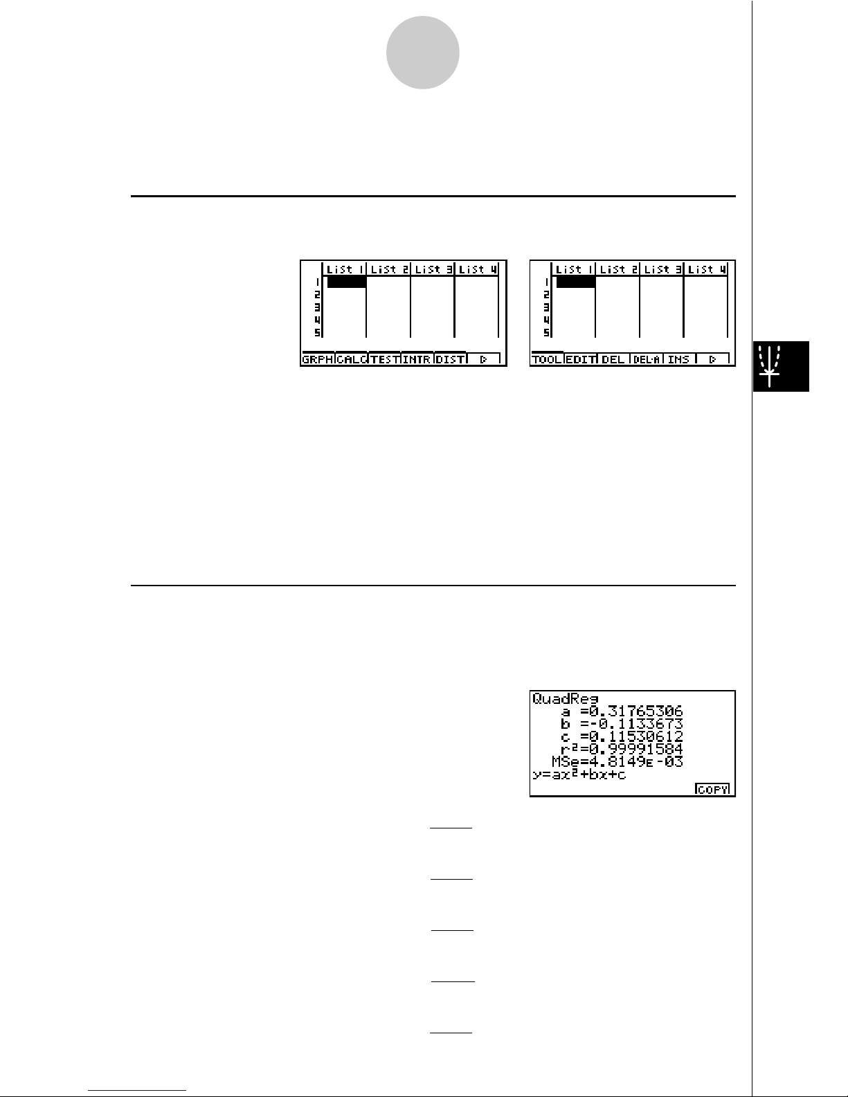
uChanges to the Function Menu

Installing STAT2 changes the function menu of the STAT Mode list input screen (initial
screen) as shown below.

Pressing a function key that corresponds to the added item displays a menu that lets you
select one of the functions listed below.

• 3(TEST) ... Test (Chapter 2, page 6)

• 4(INTR) ... Confidence interval (Chapter 3, page 31)

• 5(DIST) ... Distribution (Chapter 4, page 42)

The SORT and JUMP functions available with ALGEBRA FX2.0 are moved to the TOOL
menu (6 and 1) by STAT2.

uu

uu

uCalculation of the Coefficient of Determination (r2) and MSE

STAT2 adds calculation of the coefficient of determination (r2) for quadratic regression, cubic
regression, and quartic regression. The following types of MSE calculations are also added
for each type of regression.

• Linear Regression ...

MSE =

!

1

n – 2

i=1

n

(yi – (axi+ b))

2

• Quadratic Regression ...

MSE =

!

1

n – 3

i=1

n

(yi – (ax

i

+ bxi+ c))

2

2

• Cubic Regression ...

MSE =

!

1

n – 4

i=1

n

(yi – (ax

i

3

+ bx

i

+ cx

i

+d ))

2

2

• Quartic Regression ...

MSE =

!

1

n – 5

i=1

n

(yi – (ax

i

4

+ bx

i3

+ cx

i

+ dx

i

+ e))

2

2

• Logarithmic Regression ...

MSE =

!

1

n – 2

i=1

n

(yi – (a + b ln xi ))

2

3

• Exponential Repression ...

MSE =

!

1

n – 2

i=1

n

(ln yi – (ln a + bxi ))

2

• Power Regression ...

MSE =

!

1

n – 2

i=1

n

(ln yi – (ln a + b ln xi ))

2

• Sin Regression ...

MSE =

!

1

n – 2

i=1

n

(yi – (a sin (bxi + c) + d ))

2

• Logistic Regression ...

MSE =

!

1

n – 2 1 + ae

-bx

i

C

i=1

n

yi –

2

uu

uu

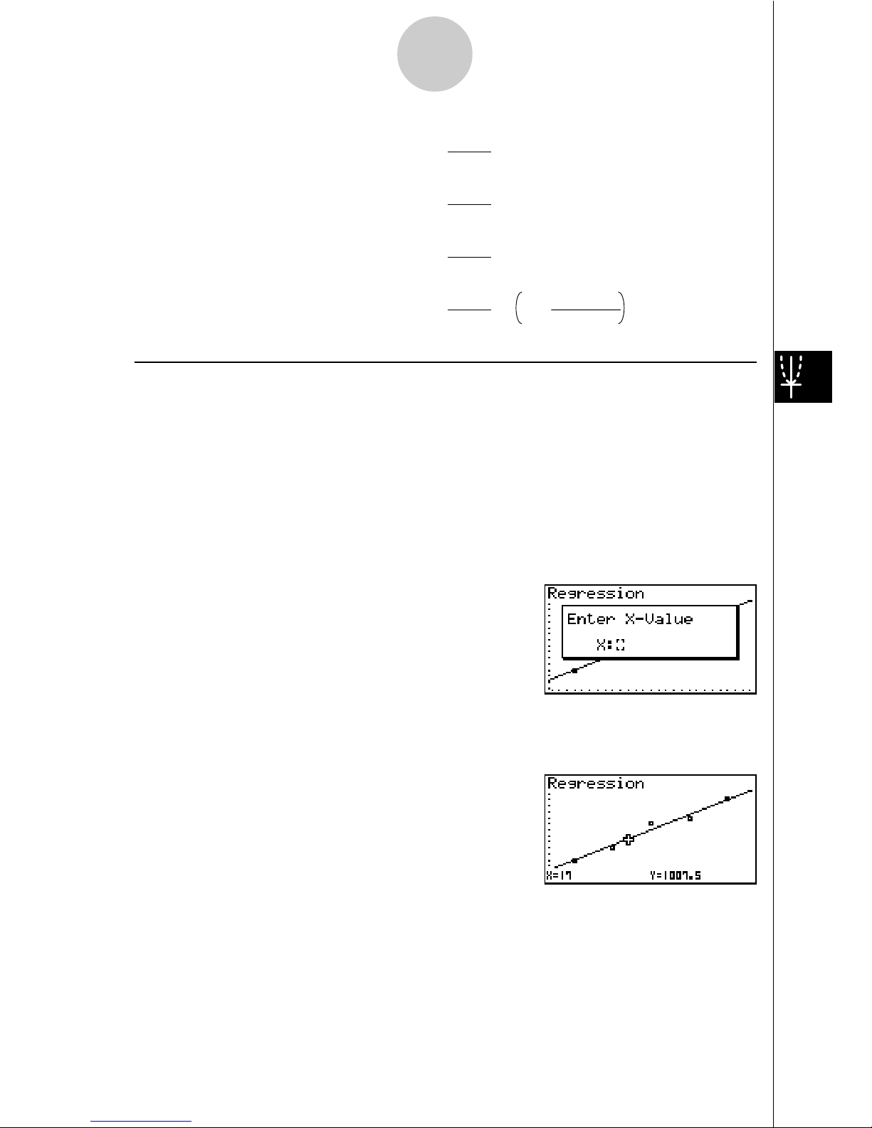
uEstimated Value Calculation for Regression Graphs

STAT2 adds a Y-CAL function that uses regression to calculate the estimated y-value for a
particular x-value after a paired-variable statistic regression graph is drawn.

The following is the general procedure for using the Y-CAL function.

1. After drawing a regression graph, press 62 (Y-CAL) to enter the graph selection mode,
and then press w.

If there are multiple graphs on the display, use f and c to select the graph you want, and
then press w.

• This causes an x-value input dialog box to appear.

2. Input the value you want for x and then press w.

• This causes the coordinates for x and y to appear at the bottom of the display, and moves
the pointer to the corresponding point on the graph.

3. Pressing v or a number key at this time causes the x-value input dialog box to reappear
so you can perform another estimated value calculation if you want.

4. After you are finished, press i to clear the coordinate values and the pointer from the
display.

· The pointer does not appear if the calculated coordinates are not within the display range.

4

· The coordinates do not appear if [Off] is specified for the [Coord] item of the [SETUP] screen.

· The Y-CAL function can also be used with a graph drawn by using DefG feature.

uu

uu

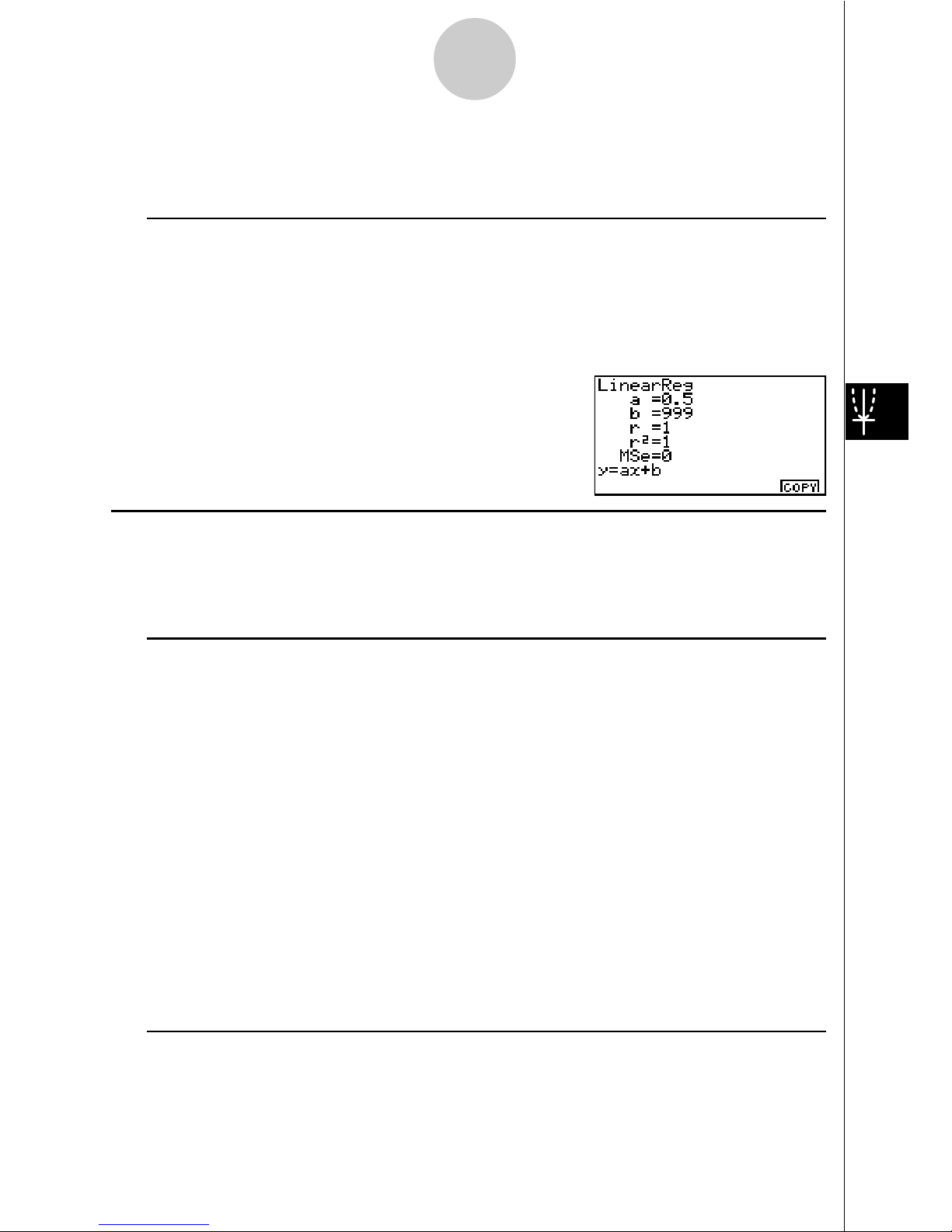
uRegression Formula Copy Function from a Regression Calculation Result

Screen

In addition to the existing regression formula copy function that lets you copy the regression
calculation result screen after drawing a statistical graph (such as Scatter Plot), STAT2 also
adds a function that lets you copy the regression formula obtained as the result of a regression
calculation. This type of copy operation is performed by pressing 6(COPY).

kk

kk

k Tests, Confidence Interval, and Distribution Calculations

STAT2 adds functions for performing tests, confidence interval, and distribution calculations.
This manual fully describes each of these calculations in separate chapters: Chapter 2 Tests,
Chapter 3 Confidence Interval, and Chapter 4 Distribution.

uu

uu

uParameter Settings

The following describes the two methods you can use to make parameter settings for test,
confidence interval, and distribution calculations.

• Selection

With this method, you press the function key that corresponds to the setting you want to
select from the function menu.

• Value Input

With this method, you directly input the parameter value you want to input. In this case,
nothing appears in the function menu.

· Pressing i returns to the list input screen, with the cursor in the same position it was at

before you started the parameter setting procedure.

· Pressing ! i (QUIT) returns to the top of list input screen.

· Pressing w without pressing 1 (CALC) under “Execute” item advances to calculation ex-

ecution. To return to the parameter setting screen, press i, A, or w.

uu

uu

uCommon Functions

• The symbol “!” appears in the upper right corner of the screen while execution of a calcula-

tion is being performed and while a graph is being drawn. Pressing A during this time
terminates the ongoing calculation or draw operation (AC Break).

• Pressing i or w while a calculation result or graph is on the display returns to the param-

eter setting screen. Pressing ! i (QUIT) returns to the top of list input screen.

5

· Pressing A while a calculation result is on the display returns to the parameter setting screen.

• Pressing u 5 (G"T) after drawing a graph switches to the parameter setting screen

(G"T function). Pressing u 5 (G"T) again returns to the graph screen.

· The G"T function is disabled whenever you change a setting on the parameter setting screen

, or when you perform a u 3 (SET UP) or ! K (V-Window) operation.

• You can perform the PICT menu's screen save or recall functions after drawing a graph.

· The ZOOM Function and SKETCH function are disabled.

The TRACE function is desabled, except for the geaph display of two-way ANOVA.

The graph screen cannot be scrolled.

• After drawing a graph, you can use a Save Result feature to save calculation results to a

specific list. Basically, all items are saved as they are displayed, except for the first line title.

· Each time you execute Save Result, any existing data in the list is replaced by the new

results.

6

2.Tests (TEST)

The Z Test provides a variety of different standardization-based tests. They make it possible
to test whether or not a sample accurately represents the population when the standard
deviation of a population (such as the entire population of a country) is known from previous
tests. Z testing is used for market research and public opinion research that need to be
performed repeatedly.

1-Sample Z Test tests for unknown population mean when the population standard
deviation is known.

2-Sample Z Test tests the equality of the means of two populations based on independent
samples when both population standard deviations are known.

1-Prop Z Test tests for an unknown proportion of successes.

2-Prop Z Test tests to compare the propotion of successes from two populations.

The t Test tests the hypothesis when the population standard deviation is unknown. The
hypothesis that is the opposite of the hypothesis being proven is called the

null hypothesis

,

while the hypothesis being proved is called the

alternative hypothesis

. The t-test is normally

applied to test the null hypothesis. Then a determination is made whether the null hypothesis
or alternative hypothesis will be adopted.

1-Sample t Test tests the hypothesis for a single unknown population mean when the
population standard deviation is unknown.

2-Sample t Test compares the population means when standard deviations are unknown.

Linear Reg t Test calculates the strength of the linear association of paired data.

!

2

Test tests hypothesis concerning the proportion of samples included in each of a number

of independent groups. Mainly, it generates cross-tabulation of two categorical variables
(such as yes, no) and evaluates the independence of these variables. It could be used, for
example, to evaluate the relationship between whether or not a driver has ever been
involved in a traffic accident and that person’s knowledge of traffic regulations.

2-Sample F Test tests the hypothesis for the ratio of sample variances. It could be used, for
example, to test the carcinogenic effects of multiple suspected factors such as tobacco use,
alcohol, vitamin deficiency, high coffee intake, inactivity, poor living habits, etc.

ANOVA tests the hypothesis that the population means of the samples are equal when there
are multiple samples. It could be used, for example, to test whether or not different combina­tions of materials have an effect on the quality and life of a final product.

One-Way ANOVA is used when there is one independent variable and one dependent
variable.

Two-Way ANOVA is used when there here are two independent variables and one depend­ent variable.

The following pages explain various statistical calculation methods based on the principles
described above. Full details concerning statistical principles and terminology can be found
in any standard general statistics textbook.

7

On the initial STAT2 Mode screen, press 3 (TEST) to display the test menu, which
contains the following items.

• 3(TEST)b(Z) ... Z Tests (p.7)

c(T) ... t Tests (p.15)

d(!2) ... !2 Test (p.23)

e(F) ... 2-Sample F Test (p.25)

f(ANOVA) ... ANOVA (p.27)

kk

kk

k Z Tests

uu

uu

uZ Test Common Functions

You can use the following graph analysis functions after drawing a graph.

• 1(Z) ... Displays z score.

Pressing 1 (Z) displays the z score at the bottom of the display, and displays the pointer at
the corresponding location in the graph (unless the location is off the graph screen).
Two points are displayed in the case of a two-tail test. Use d and e to move the pointer.
Press i to clear the z score.

• 2(P) ... Displays p-value.

Pressing 2 (P) displays the p-value at the bottom of the display without displaying the
pointer.
Press i to clear the p-value.

uu

uu

u1-Sample Z Test

This test is used when the sample standard deviation for a population is known to test the
hypothesis. The 1-Sample Z Test is applied to normal distribution.

Z =

o –

0

"

µ

n

o : mean of sample

µ

o : assumed population mean

"

: population standard deviation

n : size of sample

# The following V-Window settings are used for

drawing the graph. Xmin = –3.2, Xmax = 3.2,
Xscale = 1, Ymin = –0.1, Ymax = 0.45, Yscale
=0.1

# Executing an analysis function automatically

stores the z and p values in alpha variables Z
and P, respectively.

8

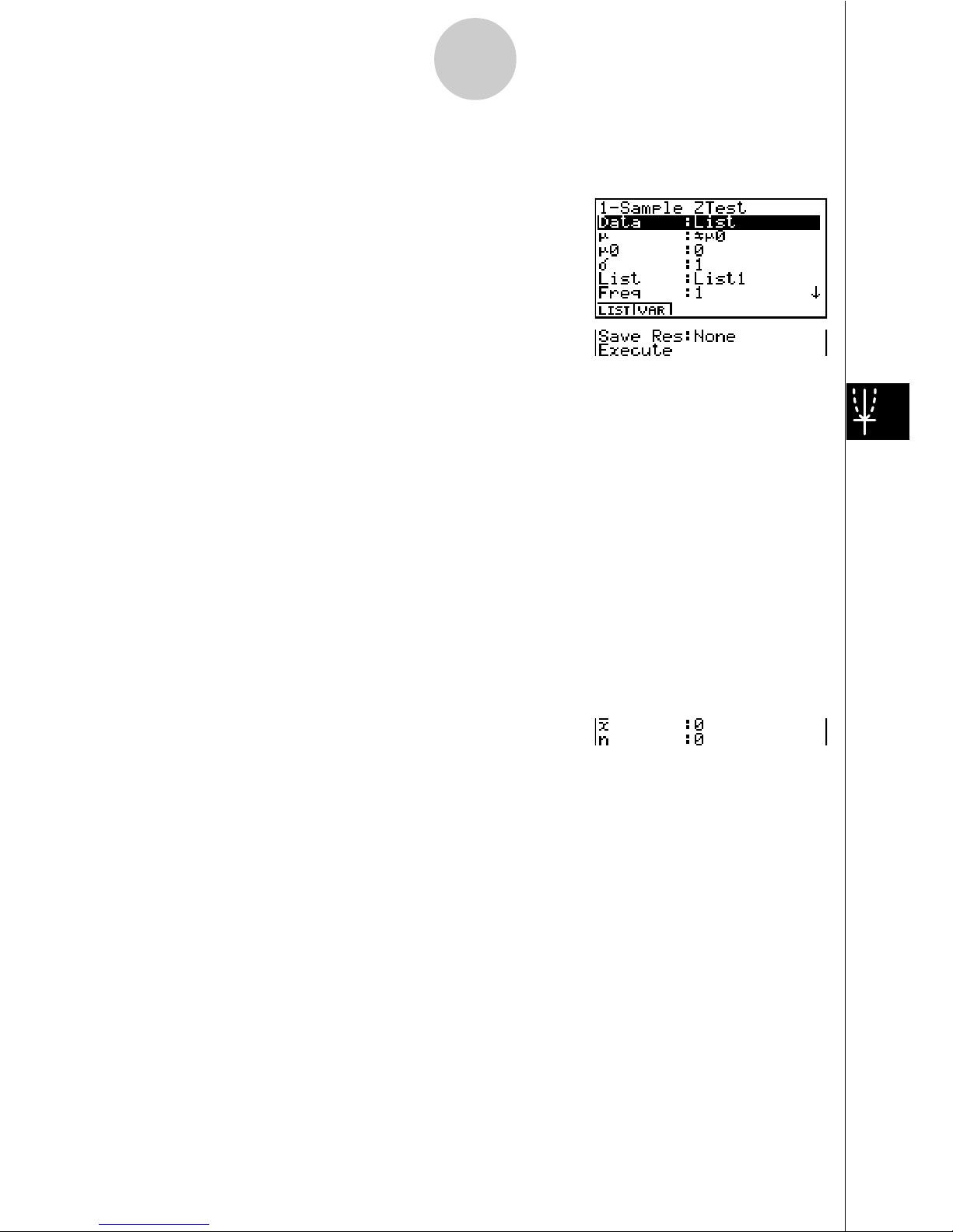
Perform the following key operation from the statistical data list.

3(TEST)

b(Z)

b(1-Smpl)

The following shows the meaning of each item in the case of list data specification.

Data ............................ data type

µ

.................................. population mean value test conditions (“G

µ

0” specifies

two-tail test, “<

µ

0” specifies lower one-tail test, “> µ0”

specifies upper one-tail test.)

µ

0 ................................. assumed population mean

!

.................................. population standard deviation (! > 0)

List .............................. list whose contents you want to use as data (List 1 to 20)

Freq ............................. frequency (1 or List 1 to 20)

Save Res .................... list for storage of calculation results (None or List 1 to 20)

Execute ....................... executes a calculation or draws a graph

The following shows the meaning of parameter data specification items that are different
from list data specification.

o .................................. mean of sample

n .................................. size of sample (positive integer)

After setting all the parameters, align the cursor with [Execute] and then press one of the
function keys shown below to perform the calculation or draw the graph.

9

• 1(CALC) ... Performs the calculation.

• 6(DRAW) ... Draws the graph.

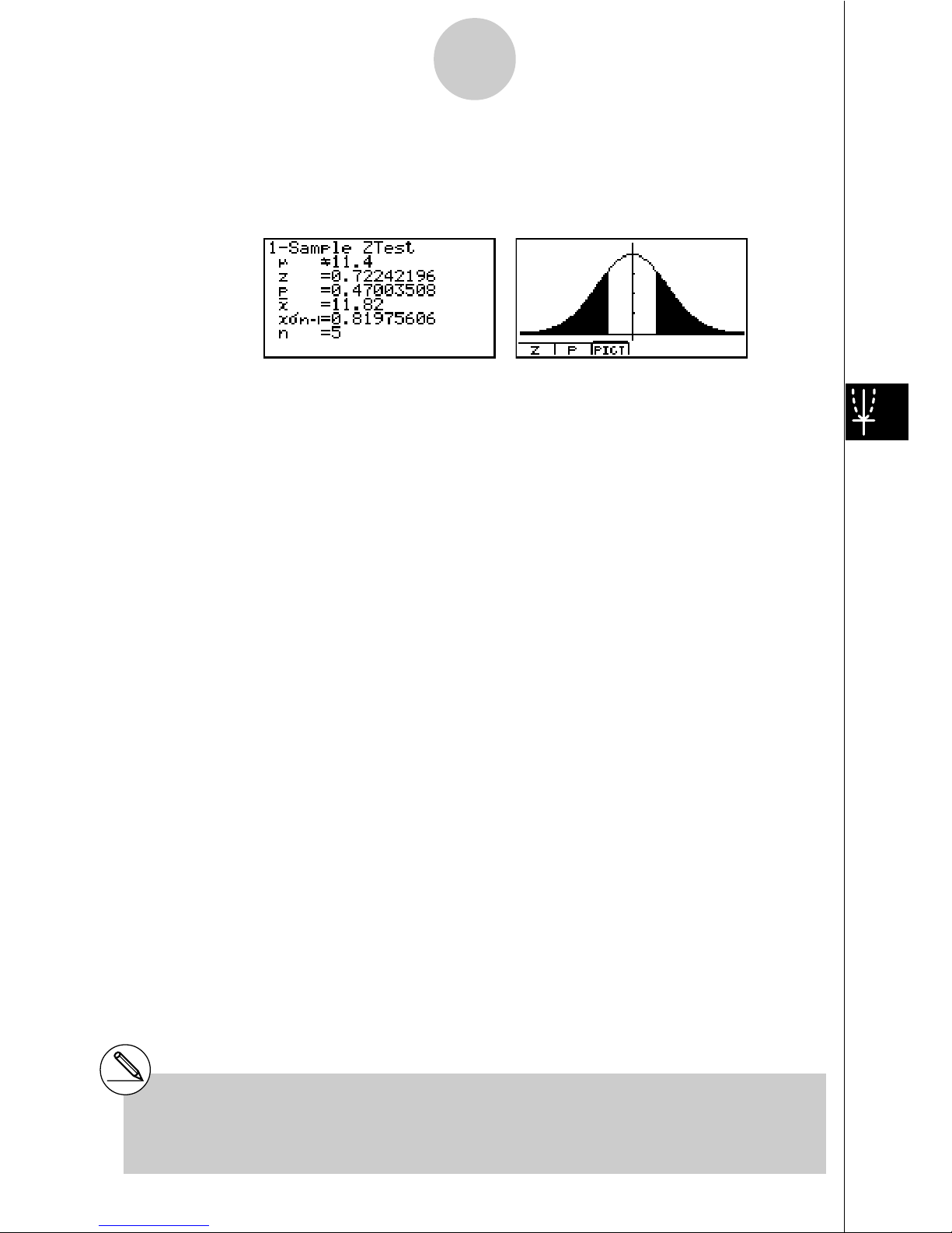
Calculation Result Output Example

µ

G11.4

........................

direction of test

z .................................. Z score

p .................................. p-value

o .................................. mean of sample

x

"

n-1 ............................. sample standard deviation

(Displayed only for Data: List setting)

n .................................. size of sample

# [Save Res] does not save the µ condition in

line 2.

10

uu

uu

u2-Sample

Z Test

This test is used when the sample standard deviations for two populations are known to test
the hypothesis. The 2-Sample Z Test is applied to normal distribution.

Z =

o1 – o

2

"

n

1

1

2

"

n

2

2

2

+

o1 : mean of sample 1
o2 : mean of sample 2

"

1 : population standard deviation of sample 1

"

2 : population standard deviation of sample 2

n1 : size of sample 1
n2 : size of sample 2

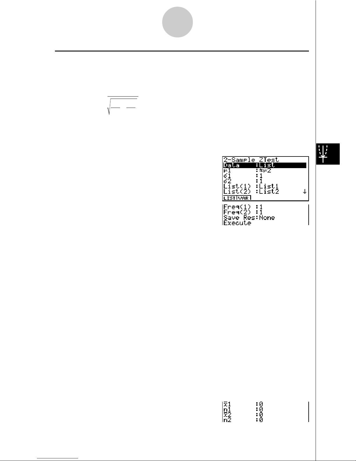
Perform the following key operation from the statistical data list.

3(TEST)

b(Z)

c(2-Smpl)

The following shows the meaning of each item in the case of list data specification.

Data ............................ data type

µ

1 ................................. population mean value test conditions (“G µ2” specifies two-

tail test, “<

µ

2” specifies one-tail test where sample 1 is

smaller than sample 2, “>

µ

2” specifies one-tail test where

sample 1 is greater than sample 2.)

"

1 ................................. population standard deviation of sample 1 ("1 > 0)

"

2 ................................. population standard deviation of sample 2 ("2 > 0)

List(1) .......................... list whose contents you want to use as sample 1 data

List(2) .......................... list whose contents you want to use as sample 2 data

Freq(1) ........................ frequency of sample 1 (positive integer)

Freq(2) ........................ frequency of sample 2 (positive integer)

Save Res .................... list for storage of calculation results (None or List 1 to 20)

Execute ....................... executes a calculation or draws a graph

The following shows the meaning of parameter data specification items that are different
from list data specification.

11

o1 ................................. mean of sample 1

n1 ................................. size (positive integer) of sample 1

o2 ................................. mean of sample 2

n2 ................................. size (positive integer) of sample 2

After setting all the parameters, align the cursor with [Execute] and then press one of the
function keys shown below to perform the calculation or draw the graph.

• 1(CALC) ... Performs the calculation.

• 6(DRAW) ... Draws the graph.

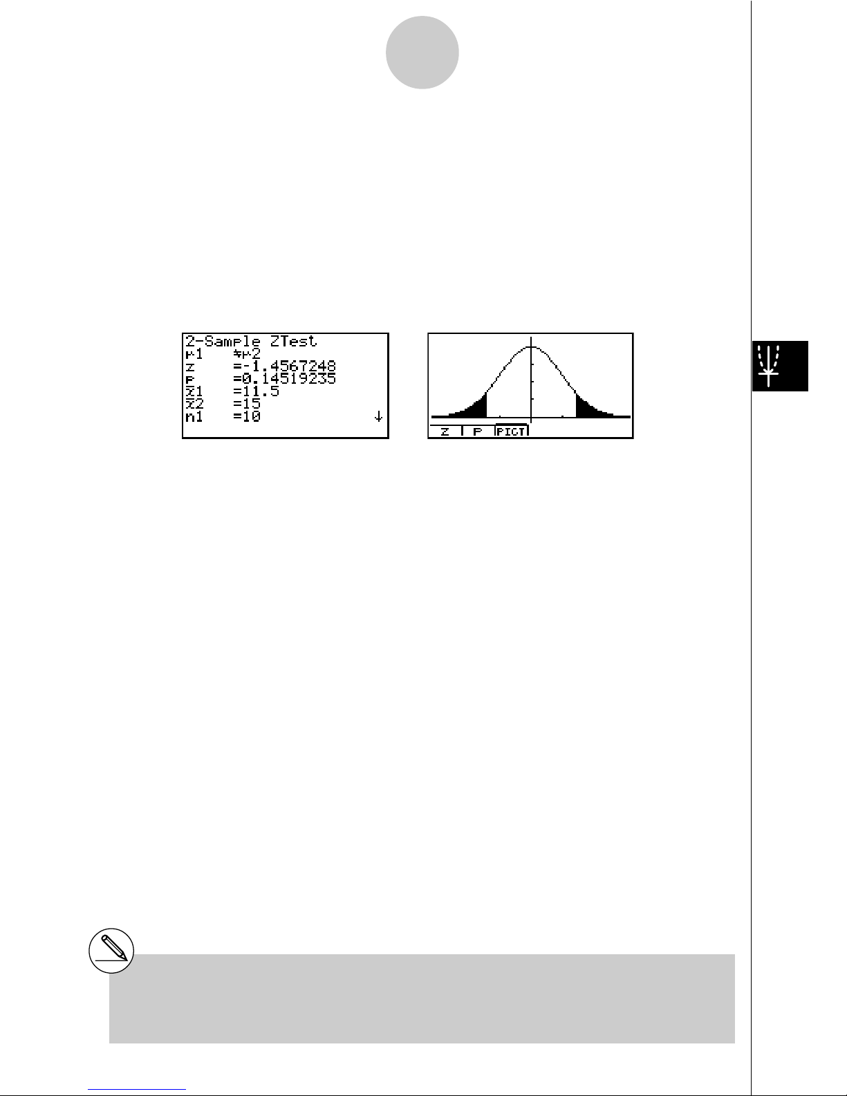
Calculation Result Output Example

µ

1

G

µ

2 ........................... direction of test

z ................................... Z score

p .................................. p-value

o1 ................................. mean of sample 1

o2 ................................. mean of sample 2

x1

"

n-1 ............................ standard deviation of sample 1

(Displayed only for Data: List Setting)

x2

"

n-1 ............................ standard deviation of sample 2

(Displayed only for Data: List Setting.)

n1 ................................. size of sample 1

n2 ................................. size of sample 2

# [Save Res] does not save the

µ

1 condition in

line 2.

12

uu

uu

u1-Prop

Z Test

This test is used to test for an unknown proportion of successes. The 1-Prop Z Test is
applied to normal distribution.

Z =

n

x

n

p

0

(1– p0)

– p

0

p0 : expected sample proportion
n : size of sample

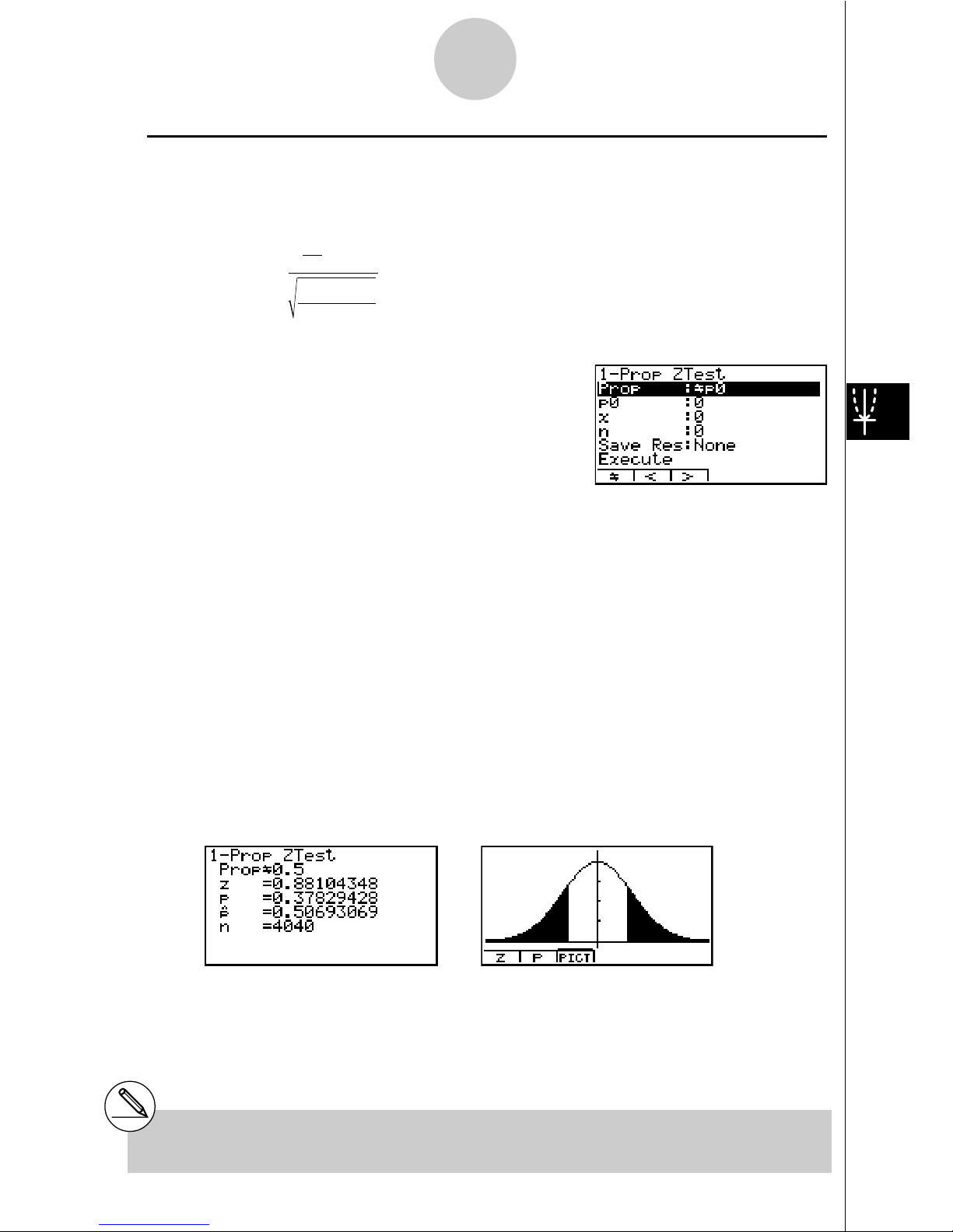
Perform the following key operation from the statistical data list.

3(TEST)

b(Z)

d(1-Prop)

Prop ............................ sample proportion test conditions (“G p0” specifies two-tail

test, “< p0” specifies lower one-tail test, “> p0” specifies upper
one-tail test.)

p0 ................................. expected sample proportion (0 < p0 < 1)

x .................................. sample value (x > 0 integer)

n .................................. size of sample (positive integer)

Save Res .................... list for storage of calculation results (None or List 1 to 20)

Execute ....................... executes a calculation or draws a graph

After setting all the parameters, align the cursor with [Execute] and then press one of the
function keys shown below to perform the calculation or draw the graph.

• 1(CALC) ... Performs the calculation.

• 6(DRAW) ... Draws the graph.

Calculation Result Output Example

PropG0.5 .................... direction of test

z ................................... Z score

p .................................. p-value

ˆp .................................. estimated sample proportion

n .................................. size of sample

# [Save Res] does not save the Prop condition

in line 2.

13

uu

uu

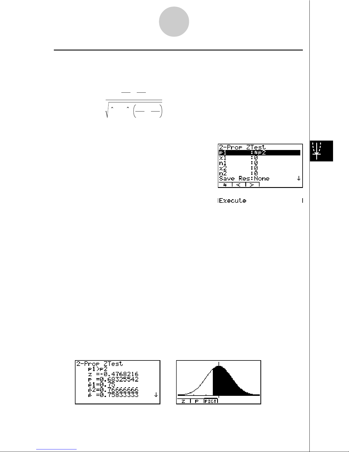
u2-Prop Z Test

This test is used to compare the proportion of successes. The 2-Prop Z Test is applied to
normal distribution.

Z =

n

1

x

1

n

2

x

2

–

p(1 – p )

n

1

1

n

2

1

+

x1 : data value of sample 1
x2 : data value of sample 2
n1 : size of sample 1
n2 : size of sample 2
ˆp : estimated sample proportion

Perform the following key operation from the statistical data list.

3(TEST)

b(Z)

e(2-Prop)

p1 ................................. sample proportion test conditions (“G p2” specifies two-tail

test, “< p2” specifies one-tail test where sample 1 is less than
sample 2, “> p2” specifies upper one-tail test where sample 1
is greater than sample 2.)

x1 ................................. data value (x1 > 0 integer) of sample 1

n1 ................................. size (positive integer) of sample 2

x2 ................................. data value (x2 > 0 integer) of sample 1

n2 ................................. size (positive integer) of sample 2

Save Res .................... list for storage of calculation results (None or List 1 to 20)

Execute ....................... executes a calculation or draws a graph

After setting all the parameters, align the cursor with [Execute] and then press one of the
function keys shown below to perform the calculation or draw the graph.

• 1(CALC) ... Performs the calculation.

• 6(DRAW) ... Draws the graph.

Calculation Result Output Example

14

p1>p2 ............................ direction of test

z .................................. Z score

p .................................. p-value

ˆp 1 ................................. estimated proportion of sample 1

ˆp 2 ................................. estimated proportion of sample 2

ˆp .................................. estimated sample proportion

n1 ................................. size of sample 1

n2 ................................. size of sample 2

# [Save Res] does not save the p1 condition in

line 2.

15

kk

kk

k t Tests

uu

uu

u t Test Common Functions

You can use the following graph analysis functions after drawing a graph.

• 1(T) ... Displays t score.

Pressing 1 (T) displays the t score at the bottom of the display, and displays the pointer at the
corresponding location in the graph (unless the location is off the graph screen).

Two points are displayed in the case of a two-tail test. Use d and e to move the pointer.

Press i to clear the t score.

• 2(P) ... Displays p-value.

Pressing 2 (P) displays the p-value at the bottom of the display without displaying the pointer.

Press i to clear the p-value.

# The following V-Window settings are used for

drawing the graph. Xmin = –3.2, Xmax = 3.2,
Xscale = 1, Ymin = –0.1, Ymax = 0.45, Yscale
=0.1

# Executing an analysis function automatically

stores the t and p values in alpha variables T
and P, respectively.

16

uu

uu

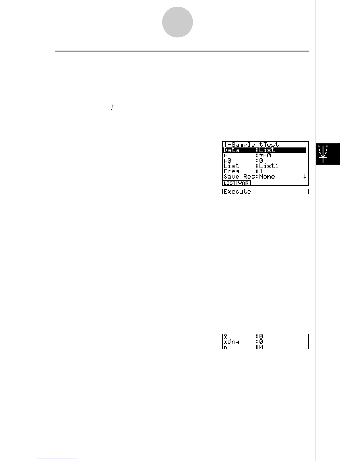
u1-Sample t Test

This test uses the hypothesis test for a single unknown population mean when the popula­tion standard deviation is unknown. The 1-Sample t Test is applied to t-distribution.

t =

o –

0

µ

"

x

n–1

n

o : mean of sample

µ

0 : assumed population mean

x

"

n-1 : sample standard deviation

n : size of sample

Perform the following key operation from the statistical data list.

3(TEST)

c(T)

b(1-Smpl)

The following shows the meaning of each item in the case of list data specification.

Data ............................ data type

µ

.................................. population mean value test conditions (“G

µ

0” specifies two-

tail test, “<

µ

0” specifies lower one-tail test, “> µ0” specifies

upper one-tail test.)

µ

0 ................................. assumed population mean

List .............................. list whose contents you want to use as data

Freq ............................. frequency

Save Res .................... list for storage of calculation results (None or List 1 to 20)

Execute ....................... executes a calculation or draws a graph

The following shows the meaning of parameter data specification items that are different
from list data specification.

o .................................. mean of sample

x

"

n-1 ............................. sample standard deviation (x"n-1 > 0)

n .................................. size of sample (positive integer)

After setting all the parameters, align the cursor with [Execute] and then press one of the
function keys shown below to perform the calculation or draw the graph.

• 1(CALC) ... Performs the calculation.

• 6(DRAW) ... Draws the graph.

17

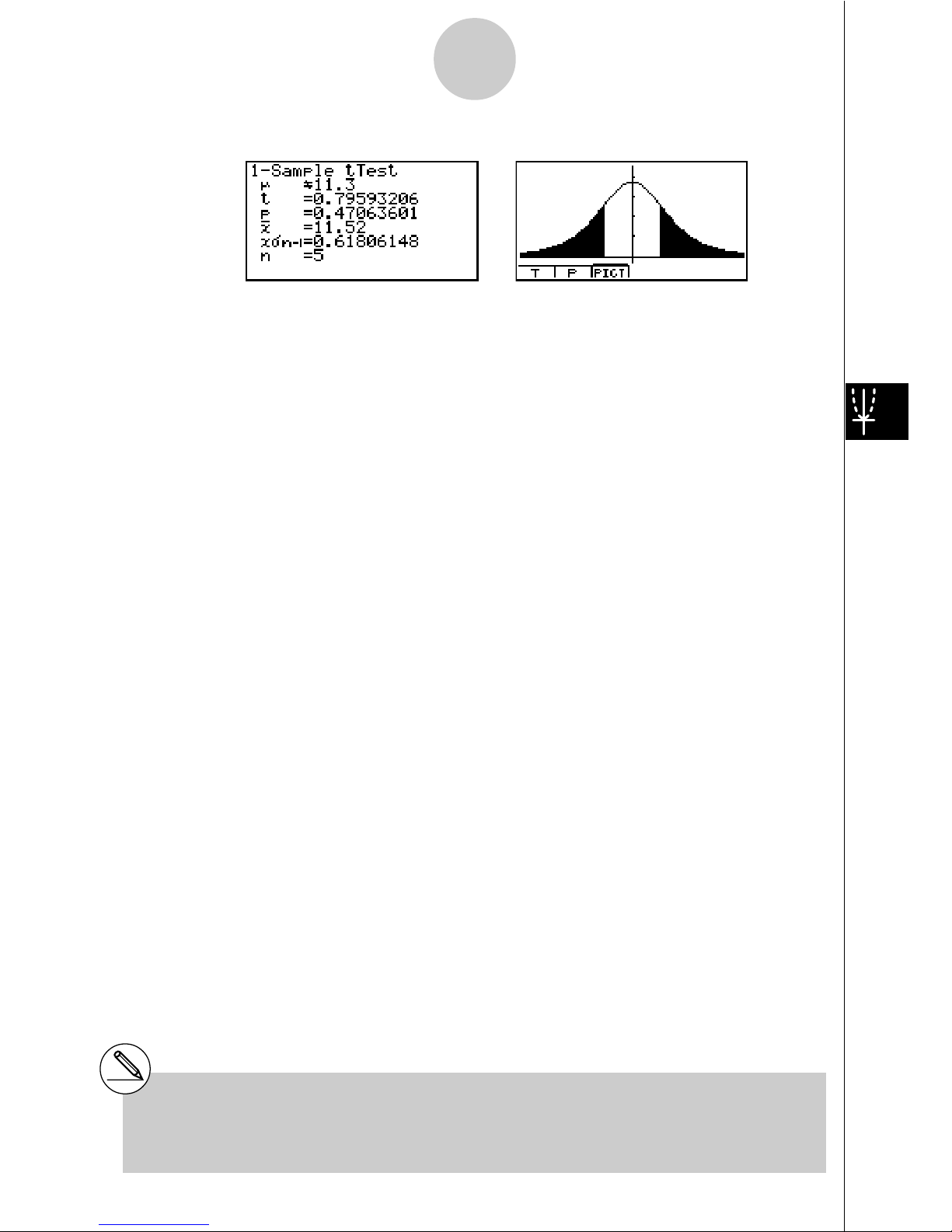
Calculation Result Output Example

µ

G 11.3 ...................... direction of test

t

...................................

t score

p .................................. p-value

o .................................. mean of sample

x

"

n-1 ............................. Sample standard deviation

n .................................. size of sample

# [Save Res] does not save the µ condition in

line 2.

18

uu

uu

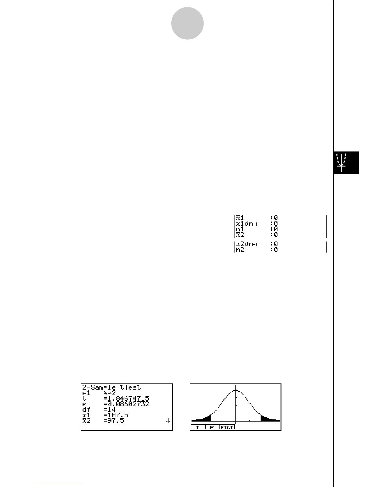
u2-Sample t Test

2-Sample t Test compares the population means when standard deviations are unknown.
The 2-Sample t Test is applied to t-distribution.

t =

o1 – o

2

x

1 n–1

2

"

n

1

+

x

2 n–1

2

"

n

2

o1 : mean of sample 1
o2 : mean of sample 2

x1

"

n-1 : standard deviation of sample 1

x2

"

n-1 : standard deviation of sample 2

n1 : size of sample 1
n2 : size of sample 2

This formula is applicable when the sample is not pooled, and the denominator is different
when the sample is pooled.

Degrees of freedom df and xp

"

n-1 differs according to whether or not pooling is in effect.

The following applies when pooling is in effect.

df

= n1 + n2 – 2

x

p n–1

=

"

n

1

+ n

2

– 2

(n

1

–1)x

1

n–1

2

+(n2–1)x

2

n–1

2

"

"

The following applies when pooling is not in effect.

df =

1

C

2

n1–1

+

(1–C )

2

n2–1

C =

x

1 n–1

2

"

n

1

+

x

2 n–1

2

"

n

2

x

1 n–1

2

"

n

1

Perform the following key operation from the statistical data list.

3(TEST)

c(T)

c(2-Smpl)

19

The following shows the meaning of each item in the case of list data specification.

Data ............................ data type

µ

1 ................................. sample mean value test conditions (“G µ2” specifies two-tail

test, “<

µ

2” specifies one-tail test where sample 1 is smaller

than sample 2, “>

µ

2” specifies one-tail test where sample 1 is

greater than sample 2.)

List(1) .......................... list whose contents you want to use as data of sample 1

List(2) .......................... list whose contents you want to use as data of sample 2

Freq(1) ........................ frequency of sample 1 (positive integer)

Freq(2) ........................ frequency of sample 2 (positive integer)

Pooled ......................... pooling On (in effect) or Off (not in effect)

Save Res .................... list for storage of calculation results (None or List 1 to 20)

Execute ....................... executes a calculation or draws a graph

The following shows the meaning of parameter data specification items that are different
from list data specification.

o1 ................................. mean of sample 1

x1

"

n-1 ............................ standard deviation (x1"n-1 > 0) of sample 1

n1 ................................. size (positive integer) of sample 2

o2 ................................. mean of sample 2

x2

"

n-1 ............................ standard deviation (x2"n-1 > 0) of sample 2

n2 ................................. size (positive integer) of sample 2

After setting all the parameters, align the cursor with [Execute] and then press one of the
function keys shown below to perform the calculation or draw the graph.

• 1(CALC) ... Performs the calculation.

• 6(DRAW) ... Draws the graph.

Calculation Result Output Example

µ1Gµ

2 ........................... direction of test

t

...................................

t score

20

p .................................. p-value

df ................................. degrees of freedom

o1 ................................. mean of sample 1

o2 ................................. mean of sample 2

x1

"

n-1 ............................ standard deviation of sample 1

x2

"

n-1 ............................ standard deviation of sample 2

xp

"

n-1 ............................ pooled sample standard deviation (Displayed only when

Pooled: On Setting.)

n1 ................................. size of sample 1

n2 ................................. size of sample 2

# [Save Res] does not save the

µ1

condition in

line 2.

21

uu

uu

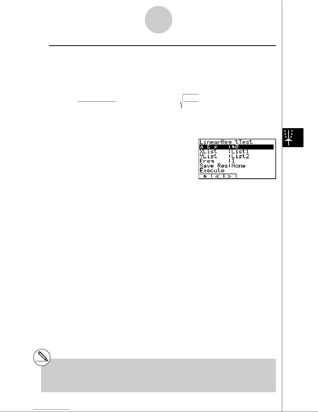
uLinearReg

t Test

LinearReg t Test treats paired-variable data sets as (x, y) pairs and plots all data on a
graph. Next, a straight line (y = a + bx) is drawn through the area where the greatest number
of plots are located and the degree to which a relationship exists is calculated.

b =

#

( x – o)( y – p)

i=1

n

#

(x – o)

2

i=1

n

a = p – bo t = r

n – 2

1 – r

2

a : intercept
b : slope of the line
n : size of sample (n>3)
r : correlation coefficient
r

2

: c

oefficient of determination

Perform the following key operation from the statistical data list.

3(TEST)

c(T)

d(LinReg)

The following shows the meaning of each item in the case of list data specification.

$

& %............................ p-value test conditions (“G 0” specifies two-tail test, “< 0”

specifies lower one-tail test, “> 0” specifies upper one-tail
test.)

XList ............................ list for x-axis data

YList ............................ list for y-axis data

Freq ............................. frequency

Save Res .................... list for storage of calculation results (None or List 1 to 20)

Execute ....................... executes a calculation

After setting all the parameters, align the cursor with [Execute] and then press the function key
shown below to perform the calculation.

• 1(CALC) ... Performs the calculation.

# You cannot draw a graph for LinearReg t

Test.

22

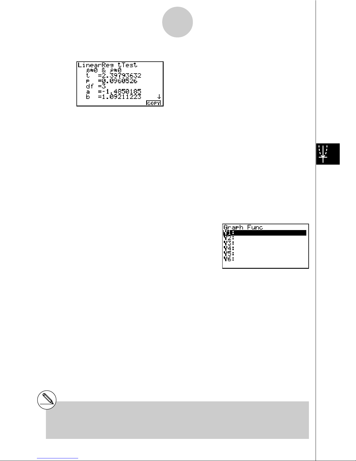
Calculation Result Output Example

$

G 0 &

%

G 0 .............. direction of test

t ................................... t score

p .................................. p-value

df ................................. degrees of freedom

a .................................. constant term

b .................................. coefficient

s .................................. standard error

r .................................. correlation coefficient

r

2

................................. coefficient of determination

Pressing 6 (COPY) while a calculation result is on the display copies the regression formula
to the graph formula editor.

When there is a list specified for the [Resid List] item on the SET UP screen, regression formula
residual data is automatically saved to the specified list after the calculation is finished.

# [Save Res] does not save the $ &

%

conditions in line 2.

# When the list specified by [Save Res] is the

same list specified by the [Resid List] item on
the SET UP screen, only[Resid List] data is
saved in the list.

23

kk

kk

k !

2

Test

!2 Test sets up a number of independent groups and tests hypothesis related to the
proportion of the sample included in each group. The !2 Test is applied to dichotomous
variables (variable with two possible values, such as yes/no).

expected counts

Fij =

#

n

#

x

ij

i=1

k

&

#

x

ij

j=1

n : all data values

!2 =

##

F

ij

i=1

k

(xij – Fij)

2

j=1

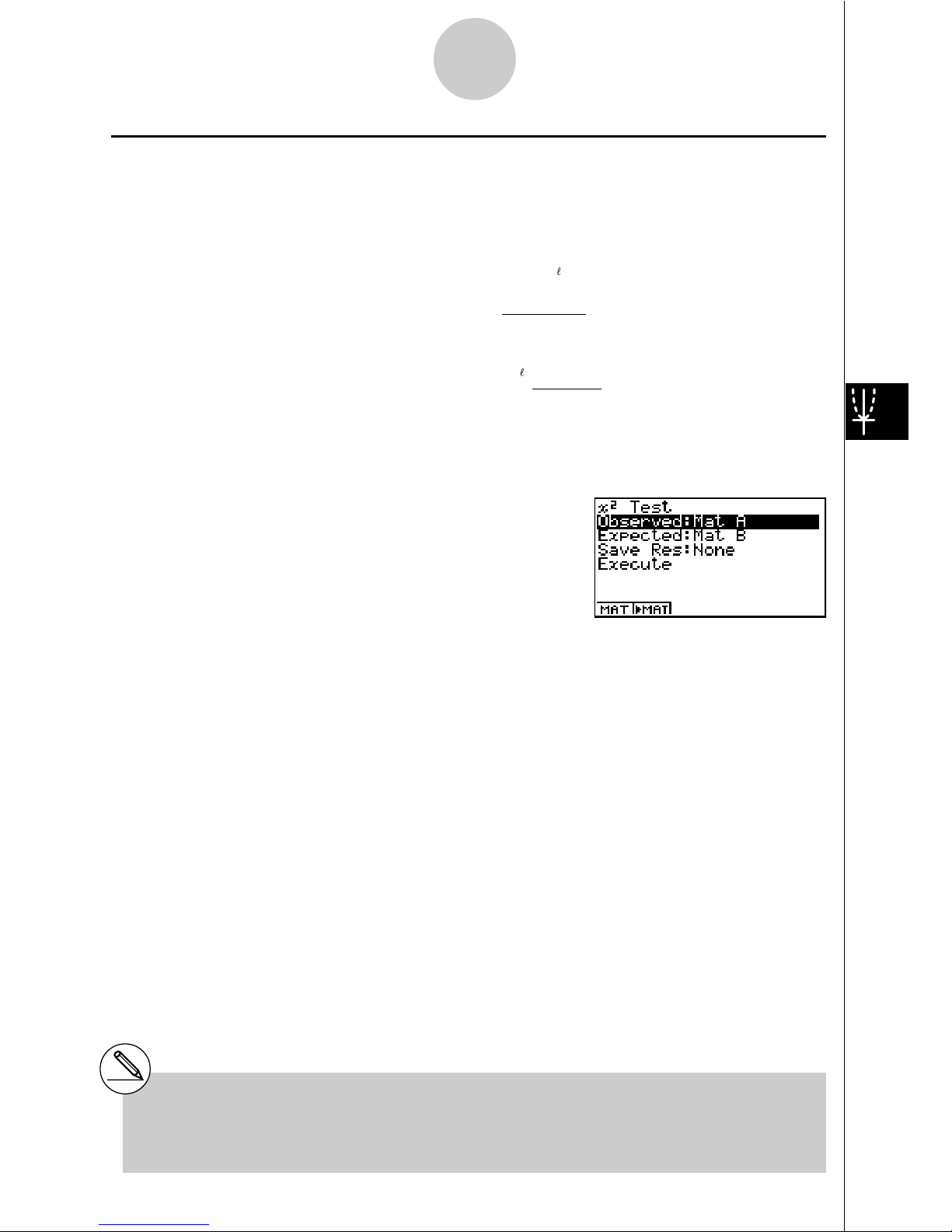
Perform the following key operation from the statistical data list.

3(TEST)

d(!2)

Next, specify the matrix that contains the data. The following shows the meaning of the
above item.

Observed .................... name of matrix (A to Z) that contains observed counts (all cells

positive integers)

Expected ..................... name of matrix (A to Z) that is for saving expected frequency

Save Res .................... list for storage of calculation results (None or List 1 to 20)

Execute ....................... executes a calculation or draws a graph

# The matrix must be at least two lines by two

columns. An error occurs if the matrix has
only one line or one column.

# Pressing 2 ('MAT) while setting

parameters enters the MATRIX editor, which
you can use to edit and view the contents of
matrices.

24

After setting all the parameters, align the cursor with [Execute] and then press one of the
function keys shown below to perform the calculation or draw the graph.

• 1(CALC) ... Performs the calculation.

• 6(DRAW) ... Draws the graph.

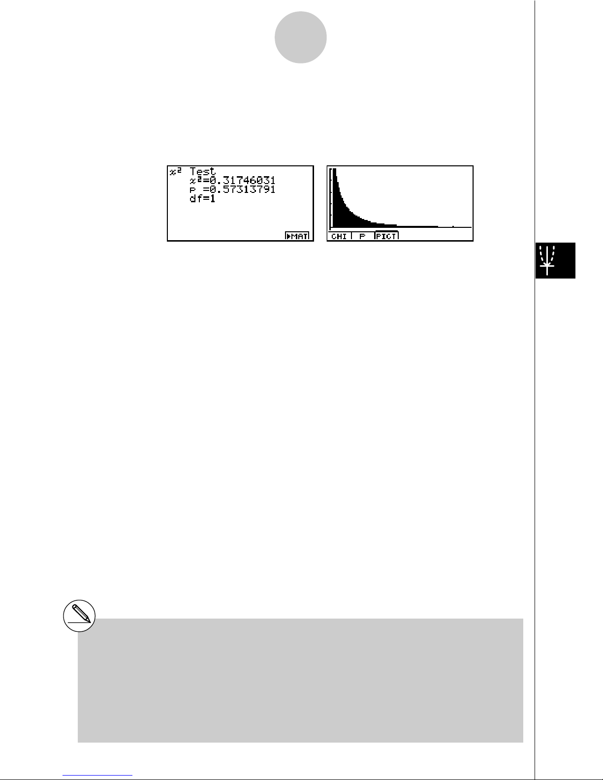
Calculation Result Output Example

!

2

................................. !2 value

p .................................. p-value

df ................................. degrees of freedom

You can use the following graph analysis functions after drawing a graph.

• 1(CHI) ... Displays

!

2

value.

Pressing 1 (CHI) displays the

!

2

value at the bottom of the display, and displays the pointer at

the corresponding location in the graph (unless the location is off the graph screen).

Press i to clear the

!

2

value.

• 2(P) ... Displays p-value.

Pressing 2 (P) displays the p-value at the bottom of the display without displaying the pointer.

Press i to clear the p-value.

# Pressing 6 (('MAT) while a calculation

result is displayed enters the MATRIX editor,
which you can use to edit and view the
contents of matrices.

# The following V-Window settings are used for

drawing the graph.Xmin = 0, Xmax = 11.5,
Xscale = 2, Ymin = –0.1, Ymax = 0.5, Yscale
=0.1

# Executing an analysis function automatically

stores the

!

2

and p values in alpha variables

C and P, respectively.

25

kk

kk

k 2-Sample F Test

2-Sample F Test tests the hypothesis for the ratio of sample variances. The F Test is
applied to F distribution.

F =

x

1 n–1

2

"

x

2 n–1

2

"

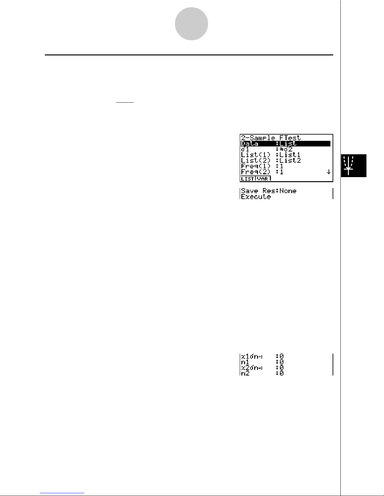
Perform the following key operation from the statistical data list.

3(TEST)

e(F)

The following is the meaning of each item in the case of list data specification.

Data ............................ data type

"

1 ................................. population standard deviation test conditions (“G "2”

specifies two-tail test, “<

"

2” specifies one-tail test where

sample 1 is smaller than sample 2, “>

"

2” specifies one-tail

test where sample 1 is greater than sample 2.)

List(1) .......................... list whose contents you want to use as data of sample 1

List(2) .......................... list whose contents you want to use as data of sample 2

Freq(1) ........................ frequency of sample 1

Freq(2) ........................ frequency of sample 2

Save Res .................... list for storage of calculation results (None or List 1 to 20)

Execute ....................... executes a calculation or draws a graph

The following shows the meaning of parameter data specification items that are different
from list data specification.

x1

"

n-1 ............................ standard deviation (x1

"

n-1

>

0) of sample 1

n1 ................................. size (positive integer) of sample 1

x2

"

n-1 ............................ standard deviation (x2

"

n-1

>

0) of sample 2

n2 ................................. size (positive integer) of sample 2

After setting all the parameters, align the cursor with [Execute] and then press one of the
function keys shown below to perform the calculation or draw the graph.

• 1(CALC) ... Performs the calculation.

• 6(DRAW) ... Draws the graph.

26

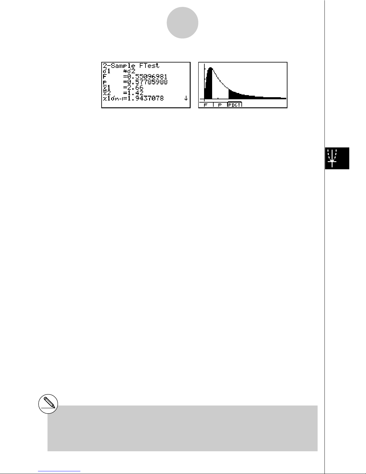
Calculation Result Output Example

"1G"

2 .......................... direction of test

F .................................. F value

p .................................. p-value

o1 ................................. mean of sample 1 (Displayed only for Data: List Setting)

o2 ................................. mean of sample 2 (Displayed only for Data: List Setting)

x1

"

n-1 ............................ standard deviation of sample 1

x2

"

n-1 ............................ standard deviation of sample 2

n1 ................................. size of sample 1

n2 ................................. size of sample 2

You can use the following graph analysis functions after drawing a graph.

• 1(F) ... Displays F value.

Pressing 1 (F) displays the F value at the bottom of the display, and displays the pointer at
the corresponding location in the graph (unless the location is off the graph screen).

Two points are displayed in the case of a two-tail test. Use d and e to move the pointer.

Press i to clear the F value.

• 2(P) ... Displays p-value.

Pressing 2 (P) displays the p-value at the bottom of the display without displaying the pointer.

Press i to clear the p-value.

# [Save Res] does not save the

"

1 condition in

line 2.

# V-Window settings are automatically

optimized for drawing the graph.

# Executing an analysis function automatically

stores the

F and p values in alpha variables

F and P, respectively

27

kk

kk

k ANOVA

ANOVA tests the hypothesis that the population means of the samples are equal when there
are multiple samples.
One-Way ANOVA is used when there is one independent variable and one dependent
variable.
Two-Way ANOVA is used when there here are two independent variables and one depend­ent variable.
This Two-Way ANOVA calculation is available under the condition that is to prepare more
than two experimental data as each dependent data.

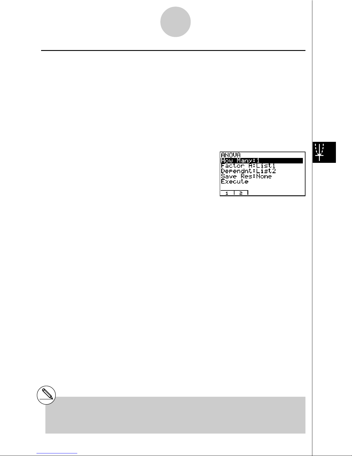
Perform the following key operation from the statistical data list.

3(TEST)

f(ANOVA)

The following is the meaning of each item in the case of list data specification.

How Many ................... selects One-Way ANOVA or Two-Way ANOVA (number of lev-

els).

Factor A....................... category list.

Dependnt .................... list to be used for sample data.

Save Res .................... first list for storage of calculation results.

Execute ....................... executes a calculation or draws a graph (Two-Way ANOVA only)

The following item appears in the case of Two-Way ANOVA only.

Factor B ...................... category list.

After setting all the parameters, align the cursor with [Execute] and then press one of the
function keys shown below to perform the calculation or draw the graph.

• 1(CALC) ... Performs the calculation.

• 6(DRAW) ... Draws the graph (Two-Way ANOVA only).

Calculation results are displayed in table form, just as they appear in science books.

# [Save Res] saves each vertical column of the

table into its own list. The leftmost column is
saved in the specified list, and each
subsequent column to the right is saved in

the next sequentially numbered list. Up to five
lists can be used for storing columns. You
can specify an first list number in the range of
1 to 16.

28

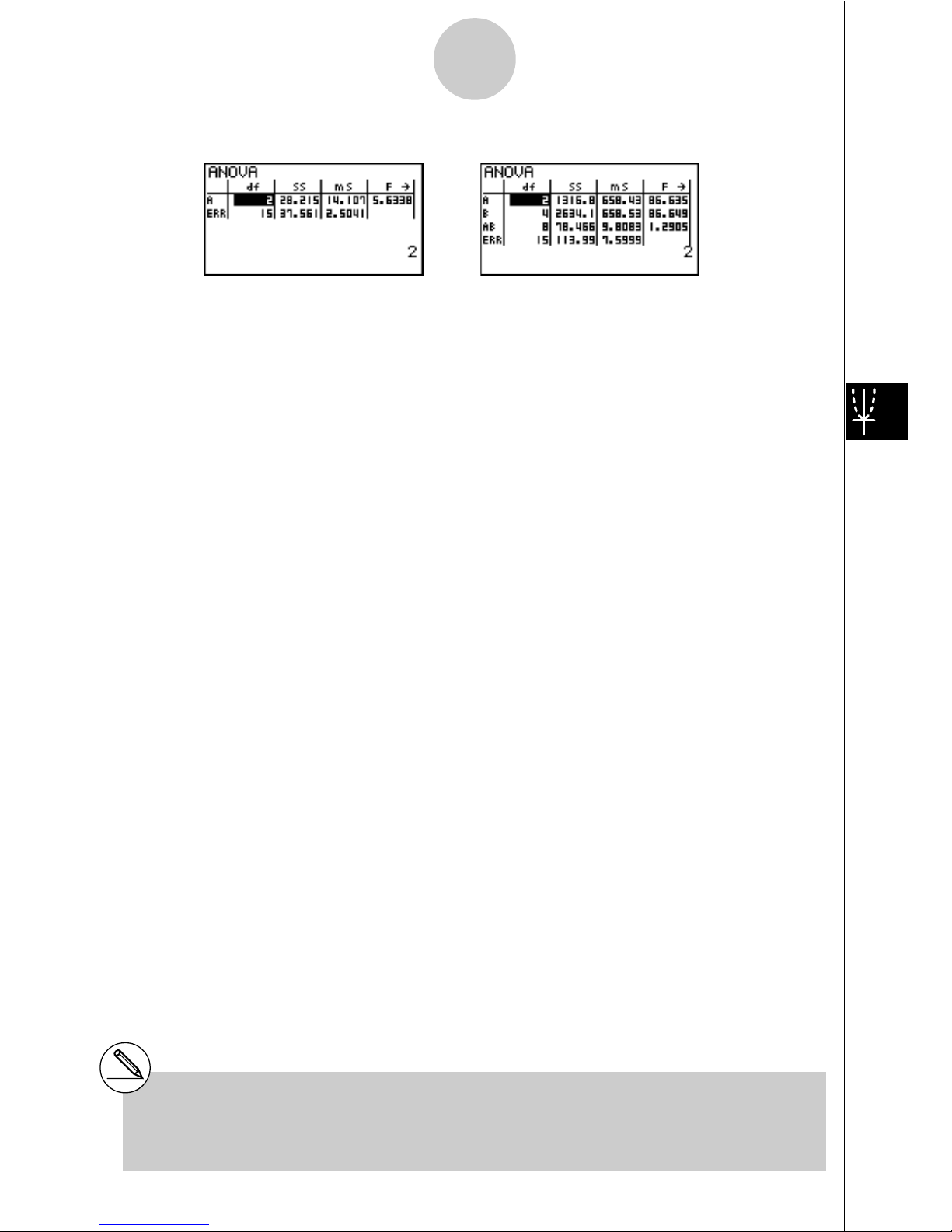
Calculation Result Output Example

One-Way ANOVA

Line 1 (A) .................... Factor A df value, SS value, MS value, F value, p-value

Line 2 (ERR) ............... Error df value, SS value, MS value

Two-Way ANOVA

Line 1 (A) .................... Factor A df value, SS value, MS value, F value, p-value

Line 2 (B) .................... Factor B df value, SS value, MS value, F value, p-value

Line 3 (AB) .................. Factor A x Factor B df value, SS value, MS value, F value,

p-value

Line 4 (ERR) ............... Error df value, SS value, MS value

F .................................. F value

p .................................. p-value

df ................................. degrees of freedom

SS ................................ sum of squares

MS ............................... mean squares

With Two-Way ANOVA, you can draw Interaction Plot graphs. The number of graphs depends
on Factor B, while the number of X-axis data depends on the Factor A. The Y-axis is the
average value of each category.

You can use the following graph analysis function after drawing a graph.

• 1(TRACE) ... Trace function

Pressing d or e moves the pointer on the graph in the corresponding direction. When there
are multiple graphs, you can move between graphs by pressing f and c.

Press i to clear the pointer from the display.

# Graphing is available with Two-Way ANOVA

only. V-Window settings are performed
automatically, regardless of SET UP screen
settings.

# Using the TRACE function automatically

stores the number of conditions to alpha
variable A and the mean value to variable M,
respectively.

29

kk

kk

k ANOVA (Two-Way)

uu

uu

uDescription

The nearby table shows measurement results for a metal product produced by a heat
treatment process based on two treatment levels: time (A) and temperature (B). The
experiments were repeated twice each under identical conditions.

Perform analysis of variance on the following null hypothesis, using a significance level of
5%.

Ho : No change in strength due to time
Ho : No change in strength due to heat treatment temperature
Ho : No change in strength due to interaction of time and heat treatment temperature

uu

uu

uSolution

Use two-way ANOVA to test the above hypothesis.
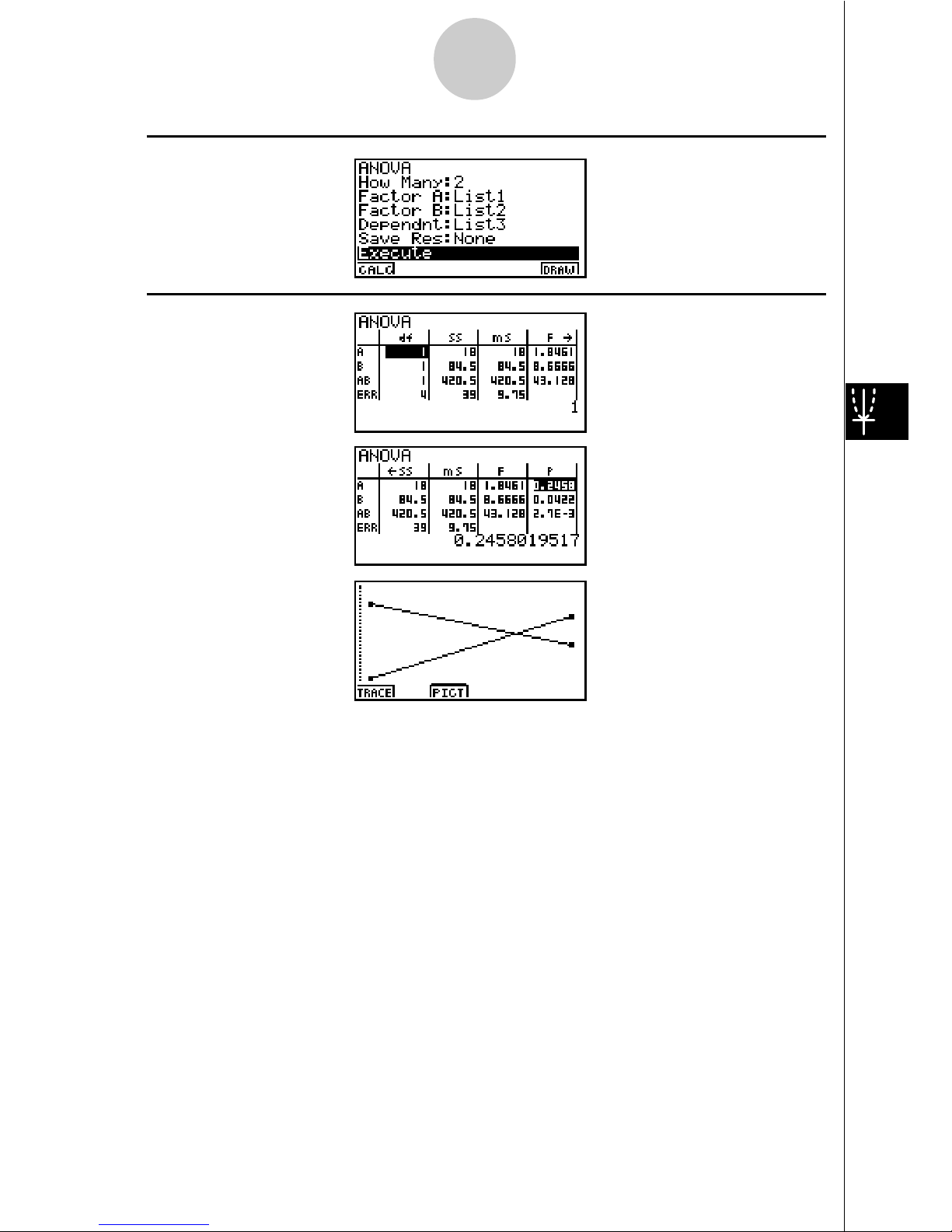
Input the above data as shown below.

List1={1,1,1,1,2,2,2,2}
List2={1,1,2,2,1,1,2,2}
List3={113,116,139,132,133,131,126,122 }

Define List 3 (the data for each group) as Dependent. Define List 1 and List 2 (the factor
numbers for each data item in List 3) as Factor A and Factor B respectively.
Executing the test produces the following results.

• Time differential (A) level of significance P = 0.2458019517
The level of significance (p = 0.2458019517) is greater than the significance level (0.05),
so the hypothesis does not reject.

• Temperature differential (B) level of significance P = 0.04222398836
The level of significance (p = 0.04222398836) is less than the significance level (0.05), so
the hypothesis rejects.

• Interaction (A & B) level of significance P = 2.78169946e-3
The level of significance (p = 2.78169946e-3) is less than the significance level (0.05), so
the hypothesis rejects.

The above test indicates that the time differential is not significant, the temperature
differential is significant, and interaction is highly significant.

B (Heat Treatment Temperature) B1 B2

A1 113 , 116

133 , 131

139 , 132

126 , 122

A2

A (Time)

30

uu

uu

uInput Example

uu

uu

uResults