Casio fx-3650P II User Manual

fx-3650P II

User's Guide

E

CASIO Worldwide Education Website

http://edu.casio.com

CASIO EDUCATIONAL FORUM

http://edu.casio.com/forum/

RJA527880-001V01

Getting Started

Thank you for purchasing this CASIO product.

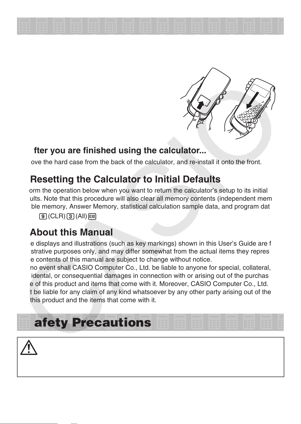
Before using the calculator for the first time...

k

Before using the calculator, slide its hard case
downwards to remove it, and then affix the hard
case to the back of the calculator as shown in the
illustration nearby.

After you are finished using the calculator...

A

Remove the hard case from the back of the calculator, and re-install it onto the front.

Resetting the Calculator to Initial Defaults

k

Perform the operation below when you want to return the calculator’s setup to its initial
defaults. Note that this procedure will also clear all memory contents (independent memory,
variable memory, Answer Memory, statistical calculation sample data, and program data).

(CLR) 3(All)

9

!

About this Manual

k

• The displays and illustrations (such as key markings) shown in this User’s Guide are for
illustrative purposes only, and may differ somewhat from the actual items they represent.

• The contents of this manual are subject to change without notice.

• In no event shall CASIO Computer Co., Ltd. be liable to anyone for special, collateral,
incidental, or consequential damages in connection with or arising out of the purchase or
use of this product and items that come with it. Moreover, CASIO Computer Co., Ltd. shall
not be liable for any claim of any kind whatsoever by any other party arising out of the use
of this product and the items that come with it.

w

Safety Precautions

Battery

• Keep batteries out of the reach of small children.

• Use only the type of battery specified for this calculator in this manual.

E-1

Operating Precautions

• Even if the calculator is operating normally, replace the battery at least once every
three years (LR44 (GPA76)).

A dead battery can leak, causing damage to and malfunction of the calculator. Never

leave a dead battery in the calculator. Do not try using the calculator while the battery is
completely dead.

• The battery that comes with the calculator discharges slightly during shipment
and storage. Because of this, it may require replacement sooner than the normal
expected battery life.

• Do not use an oxyride battery* or any other type of nickel-based primary
battery with this product. Incompatibility between such batteries and product
specifications can result in shorter battery life and product malfunction.

• Low battery power can cause memory contents to become corrupted or lost
completely. Always keep written records of all important data.

• Avoid use and storage of the calculator in areas subjected to temperature
extremes, and large amounts of humidity and dust.

• Do not subject the calculator to excessive impact, pressure, or bending.

• Never try to take the calculator apart.

• Use a soft, dry cloth to clean the exterior of the calculator.

• Whenever discarding the calculator or batteries, be sure to do so in accordance
with the laws and regulations in your particular area.

• Be sure to keep all user documentation handy for future reference.

* Company and product names used in this manual may be registered trademarks or

trademarks of their respective owners.

E-2

Contents

Getting Started ..........................................................................................1

Safety Precautions ...................................................................................1

Operating Precautions .............................................................................2

Before starting a calculation... ................................................................4

Calculation Modes and Setup .................................................................5

Inputting Calculation Expressions and Values ......................................7

Basic Calculations .................................................................................. 11

Calculation History and Replay .............................................................13

Calculator Memory Operations .............................................................14

Scientifi c Function Calculations ..........................................................17

Using 10

Complex Number Calculations (CMPLX) .............................................25

3

Engineering Notation (ENG) .................................................25

Statistical Calculations (SD/REG) .........................................................29

Base-

Program Mode (PRGM) ..........................................................................43

Appendix .................................................................................................53

Power Requirements ..............................................................................57

Specifi cations .........................................................................................58

Calculations (BASE) ..................................................................40

n

E-3

Before starting a calculation...

Turning On the Calculator

k

Press O. The calculator will enter the calculation mode (page 5) that it was in the last time
you turned it off.

Adjusting Display Contrast

A

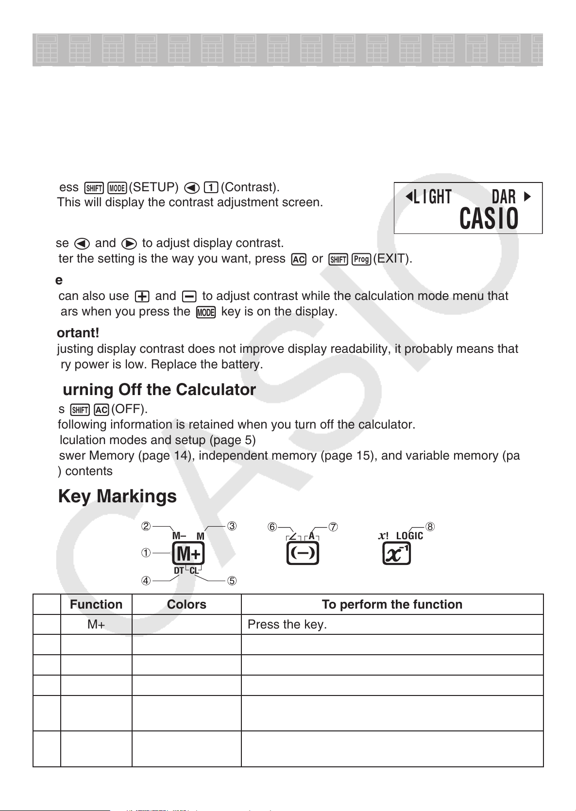
If the figures on the display become hard to read, try adjusting display contrast.

1. Press

• This will display the contrast adjustment screen.

!N

(SETUP)

d

(Contrast).

b

L IGHT DARK

CASIO

2. Use d and e to adjust display contrast.

3. After the setting is the way you want, press A or

!p

Note

You can also use + and - to adjust contrast while the calculation mode menu that
appears when you press the

key is on the display.

,

Important!

If adjusting display contrast does not improve display readability, it probably means that
battery power is low. Replace the battery.

(EXIT).

Turning Off the Calculator

A

Press
The following information is retained when you turn off the calculator.

• Calculation modes and setup (page 5)

• Answer Memory (page 14), independent memory (page 15), and variable memory (page

k

!A

16) contents

Key Markings

Function Colors To perform the function

1

2

3

(OFF).

M–

M

CL

DT

M+ Press the key.

M– Text: Amber Press

M Text: Red Press

A

and then press the key.

!

and then press the key.

a

8

LOGIC

x

!

4

5

6

DT Text: Blue In the SD or REG Mode, press the key.

CL Text: Amber

Frame: Blue

∠

Text: Amber
Frame: Purple

In the SD or REG Mode, press
the key.

In the CMPLX Mode, press
key.

!

and then press

!

and then press the

E-4

Function Colors To perform the function

7

8

Reading the Display

k

Input Expressions and Calculation Results

A

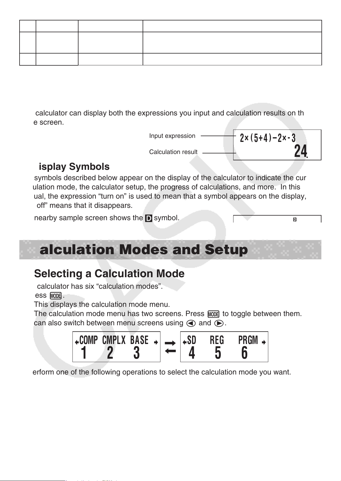
This calculator can display both the expressions you input and calculation results on the
same screen.

Display Symbols

A

The symbols described below appear on the display of the calculator to indicate the current
calculation mode, the calculator setup, the progress of calculations, and more. In this
manual, the expression “turn on” is used to mean that a symbol appears on the display, and
“turn off” means that it disappears.

A Text: Red

Frame: Green

LOGIC Text: Green In the BASE Mode, press the key.

Press
In the BASE Mode, press the key.

Input expression

Calculation result

and then press the key (variable A).

a

(

×

2

24

5+4

)

×

–

-

2

3

The nearby sample screen shows the 7 symbol.

Calculation Modes and Setup

Selecting a Calculation Mode

k

Your calculator has six “calculation modes”.

1. Press

• This displays the calculation mode menu.

• The calculation mode menu has two screens. Press
can also switch between menu screens using d and e.

2. Perform one of the following operations to select the calculation mode you want.

(COMP): COMP(Computation)

b

(BASE): BASE (Base

d

,

.

COMP CMPLX BASE

1 2 3

n

to toggle between them. You

,

SD REG PRGM

4 5 6

(CMPLX): CMPLX (Complex Number)

c

(SD): SD (Single Variable Statistics)

)

e

(REG): REG (Paired Variable Statistics)

f

• Pressing a number key from b to g selects the applicable mode, regardless of which
menu screen is currently displayed.

(PRGM): PRGM (Program)

g

E-5

Calculator Setup

k

The calculator setup can be used to configure input and output settings, calculation
parameters, and other settings. The setup can be configured using setup screens, which
you access by pressing
d and e to navigate between them.

Specifying the Angle Unit

A

90˚ =

π

radians = 100 grads

2

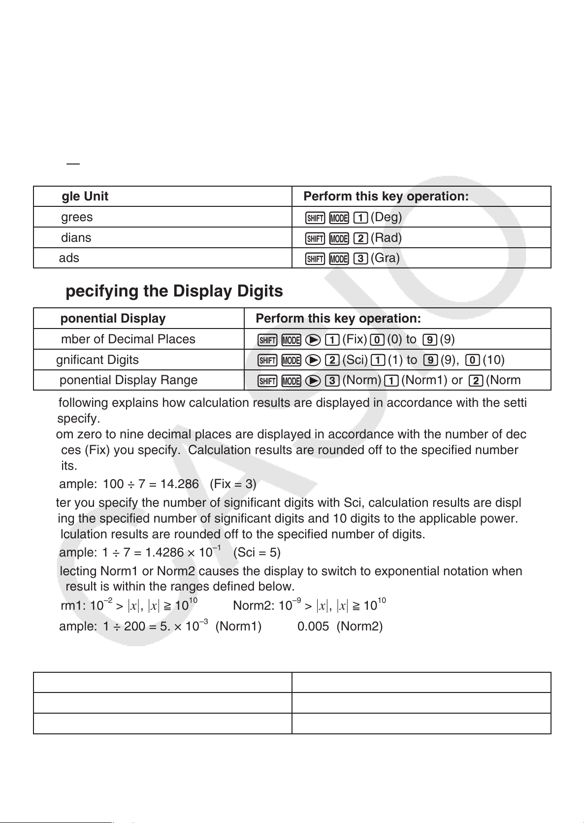
Angle Unit Perform this key operation:

!,

(SETUP). There are six setup screens, and you can use

Degrees

Radians

Grads

Specifying the Display Digits

A

Exponential Display Perform this key operation:

Number of Decimal Places

Significant Digits

Exponential Display Range

The following explains how calculation results are displayed in accordance with the setting
you specify.

• From zero to nine decimal places are displayed in accordance with the number of decimal
places (Fix) you specify. Calculation results are rounded off to the specified number of
digits.

Example: 100 ÷ 7 = 14.286 (Fix = 3)

• After you specify the number of significant digits with Sci, calculation results are displayed
using the specified number of significant digits and 10 digits to the applicable power.
Calculation results are rounded off to the specified number of digits.

–1

Example: 1 ÷ 7 = 1.4286 × 10

(Sci = 5)

!, e

!, e

!, e

!,

!,

!,

b (Deg)

c (Rad)

d (Gra)

b (Fix)a (0) to j (9)

c (Sci)b (1) to j (9), a (10)

d (Norm)

(Norm1) or c (Norm2)

b

• Selecting Norm1 or Norm2 causes the display to switch to exponential notation whenever
the result is within the ranges defined below.

–2

x

x

,

Norm1: 10

Example: 1 ÷ 200 = 5. × 10

Specifying the Fraction Display Format

A

Fraction Format Perform this key operation:

Mixed Fractions

Improper Fractions

>









> 10

10

Norm2: 10

–3

(Norm1) 0.005 (Norm2)

–9

x

x

,

>







!, ee

!, ee

> 10



10

b (ab/c)

c (d/c)

E-6

Specifying the Complex Number Display Format

A

Complex Number Format Perform this key operation:

Rectangular Coordinates

!, eee

b (

a + b

i )

Polar Coordinates

Specifying the Statistical Frequency Setting

A

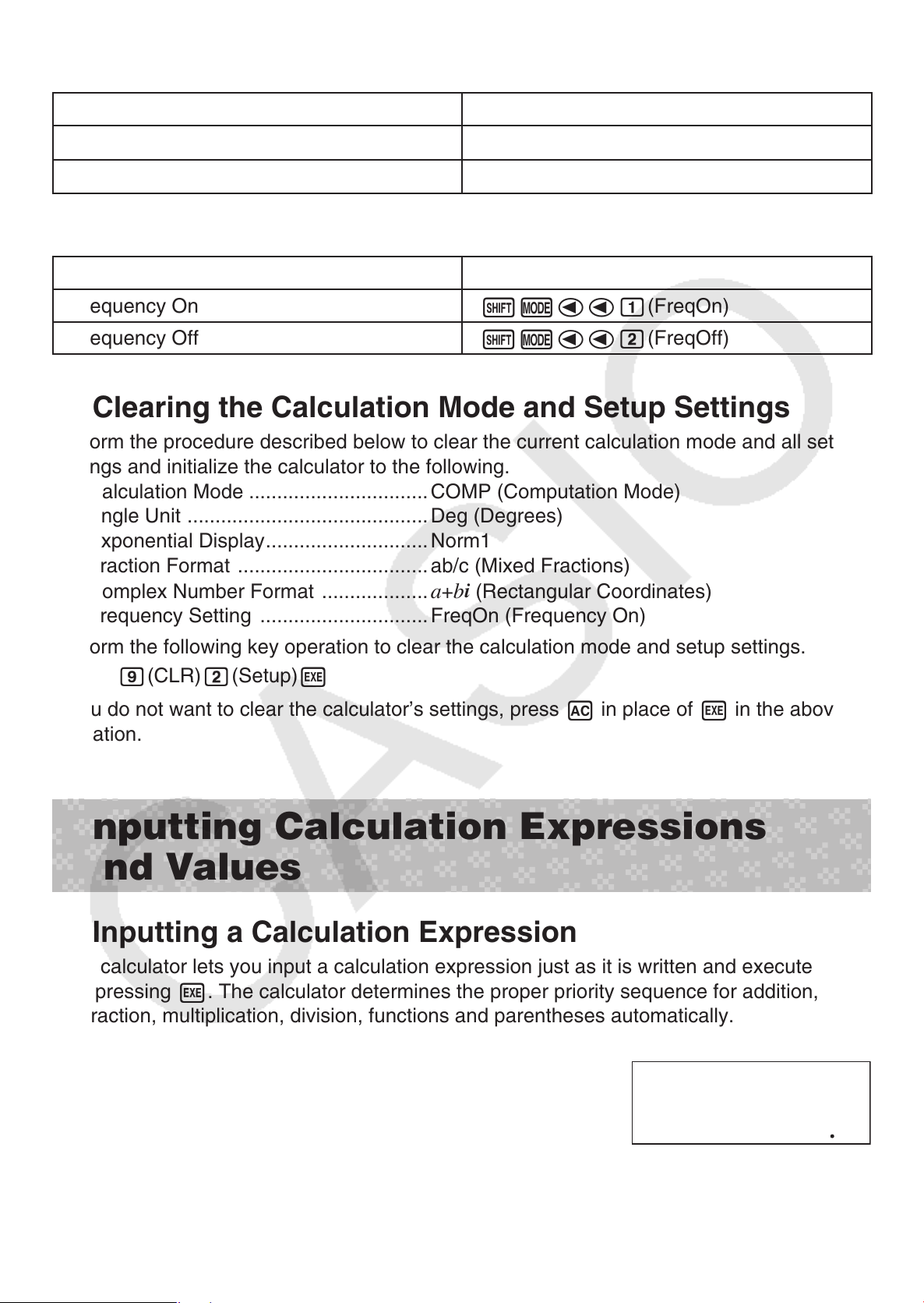
Frequency Setting Perform this key operation:

Frequency On

Frequency Off

Clearing the Calculation Mode and Setup Settings

k

Perform the procedure described below to clear the current calculation mode and all setup
settings and initialize the calculator to the following.

Calculation Mode ................................COMP (Computation Mode)

Angle Unit ........................................... Deg (Degrees)

Exponential Display ............................. Norm1

Fraction Format ..................................ab/c (Mixed Fractions)

Complex Number Format ...................

Frequency Setting .............................. FreqOn (Frequency On)

Perform the following key operation to clear the calculation mode and setup settings.

a + b

!, eee

!, dd

!, dd

i

(Rectangular Coordinates)

b (FreqOn)

c (FreqOff)

c (

r

∠  )

!

If you do not want to clear the calculator’s settings, press A in place of w in the above
operation .

w

(CLR) 2(Setup)

9

Inputting Calculation Expressions
and Values

Inputting a Calculation Expression

k

Your calculator lets you input a calculation expression just as it is written and execute
it by pressing w. The calculator determines the proper priority sequence for addition,
subtraction, multiplication, division, functions and parentheses automatically.

Example: 2 × (5 + 4) – 2 × (–3) =

2*(5+4)-

2*-3

w

(

×

2

24

5+4

)

×

-

–

2

3

E-7

Inputting Scientific Functions with Parentheses (sin, cos,

A

'

etc.)

Your calculator supports input of the scientific functions with parentheses shown below.
Note that after you input the argument, you need to press ) to close the parentheses.

sin(, cos(, tan(, sin

e

^(, 10^(, ' (, 3 ' (, Abs(, Pol(, Rec(, arg(, Conjg(, Not(, Neg(, Rnd(, ∫(, d/dx(

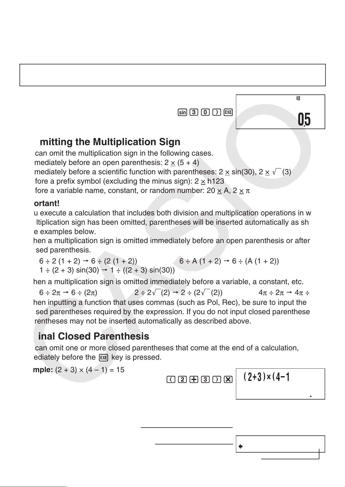
Example: sin 30 =

Omitting the Multiplication Sign

A

You can omit the multiplication sign in the following cases.

• Immediately before an open parenthesis: 2 × (5 + 4)

• Immediately before a scientific function with parentheses: 2 × sin(30), 2 × '(3)

• Before a prefix symbol (excluding the minus sign): 2 × h123

• Before a variable name, constant, or random number: 20 × A, 2 ×

–1

(, cos

–1

(, tan

–1

(, sinh(, cosh(, tanh(, sinh

30)

s

–1

(, cosh

w

–1

(, tanh

sin(30

05

π

–1

(, log(, ln(,

)

,

Important!

If you execute a calculation that includes both division and multiplication operations in which
a multiplication sign has been omitted, parentheses will be inserted automatically as shown
in the examples below.

• When a multiplication sign is omitted immediately before an open parenthesis or after a
closed parenthesis.

6 ÷ 2 (1 + 2) p 6 ÷ (2 (1 + 2)) 6 ÷ A (1 + 2) p 6 ÷ (A (1 + 2))
1 ÷ (2 + 3) sin(30) p 1 ÷ ((2 + 3) sin(30))

• When a multiplication sign is omitted immediately before a variable, a constant, etc.

6 ÷ 2π p 6 ÷ (2π) 2 ÷ 2'(2) p 2 ÷ (2'(2)) 4π ÷ 2π p 4π ÷ (2π)

• When inputting a function that uses commas (such as Pol, Rec), be sure to input the
closed parentheses required by the expression. If you do not input closed parentheses,
parentheses may not be inserted automatically as described above.

Final Closed Parenthesis

A

You can omit one or more closed parentheses that come at the end of a calculation,
immediately before the w key is pressed.

Example: (2 + 3) × (4 – 1) = 15

(2+3)*

(4-1

w

(

15

2+3

)×(

4–1

Scrolling the Screen Left and Right

A

Input Expression 12345 + 12345 + 12345

Displayed Expression

E-8

345+12345+12345I

Cursor

• While the b symbol is on the screen, you can use the d key to move the cursor to the
left and scroll the screen.

• Scrolling to the left causes part of the expression to run off the right side of the display,
which is indicated by the \ symbol on the right. While the \ symbol is on the screen,
you can use the e key to move the cursor to the right and scroll the screen.

• You can also press f to jump to the beginning of the expression, or c to jump to the
end.

Number of Input Characters (Bytes)

A

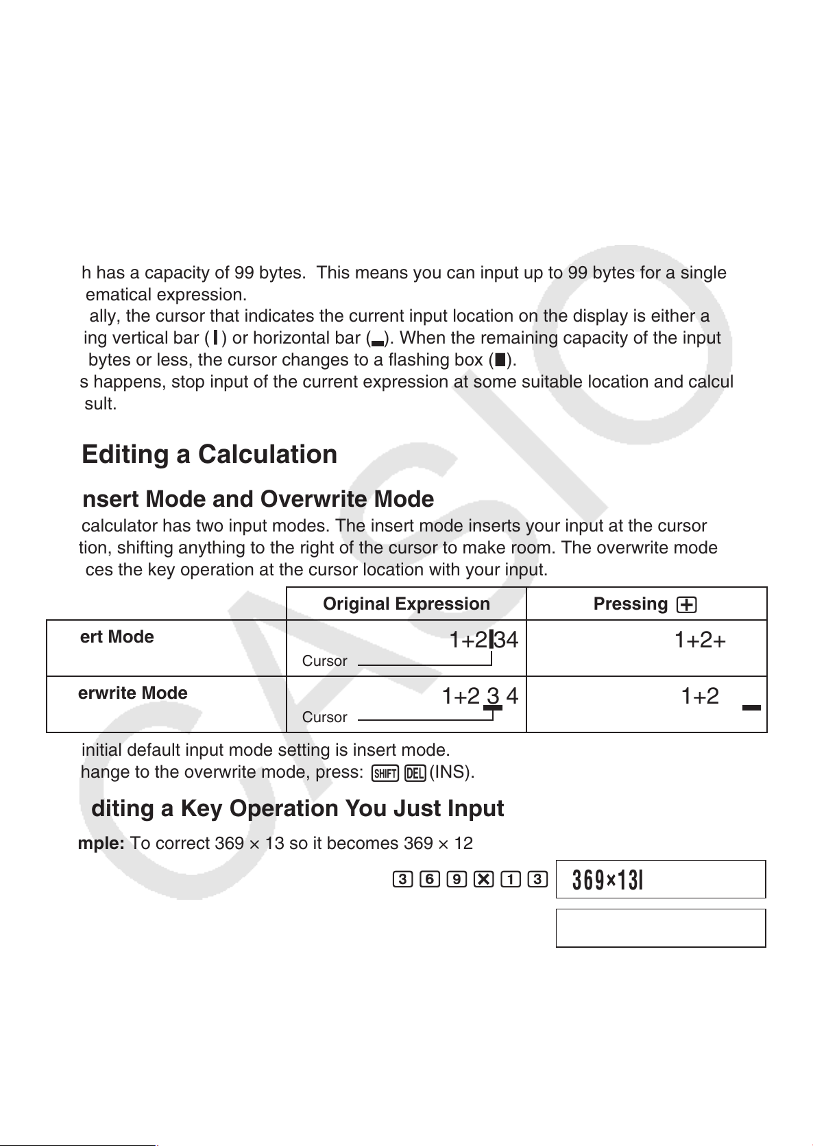
As you input a mathematical expression, it is stored in memory called an “input area,”
which has a capacity of 99 bytes. This means you can input up to 99 bytes for a single
mathematical expression.
Normally, the cursor that indicates the current input location on the display is either a
flashing vertical bar (
is 10 bytes or less, the cursor changes to a flashing box (
If this happens, stop input of the current expression at some suitable location and calculate
its result.

) or horizontal bar ( ). When the remaining capacity of the input area

|

).

k

Editing a Calculation

k

Insert Mode and Overwrite Mode

A

The calculator has two input modes. The insert mode inserts your input at the cursor
location, shifting anything to the right of the cursor to make room. The overwrite mode
replaces the key operation at the cursor location with your input.

Original Expression Pressing

Insert Mode

Cursor

Overwrite Mode

Cursor

The initial default input mode setting is insert mode.
To change to the overwrite mode, press:

Editing a Key Operation You Just Input

A

Example: To correct 369 × 13 so it becomes 369 × 12

1D

369*13

1+2 3 4

(INS).

1+2

|

34

369×13I

+

1+2+ | 34

1+2 + 4

E-9

D

2

369×12I

Deleting a Key Operation

A

Example: To correct 369 × × 12 so it becomes 369 × 12

Insert Mode

369**12

××

369

12I

ddD

Overwrite Mode

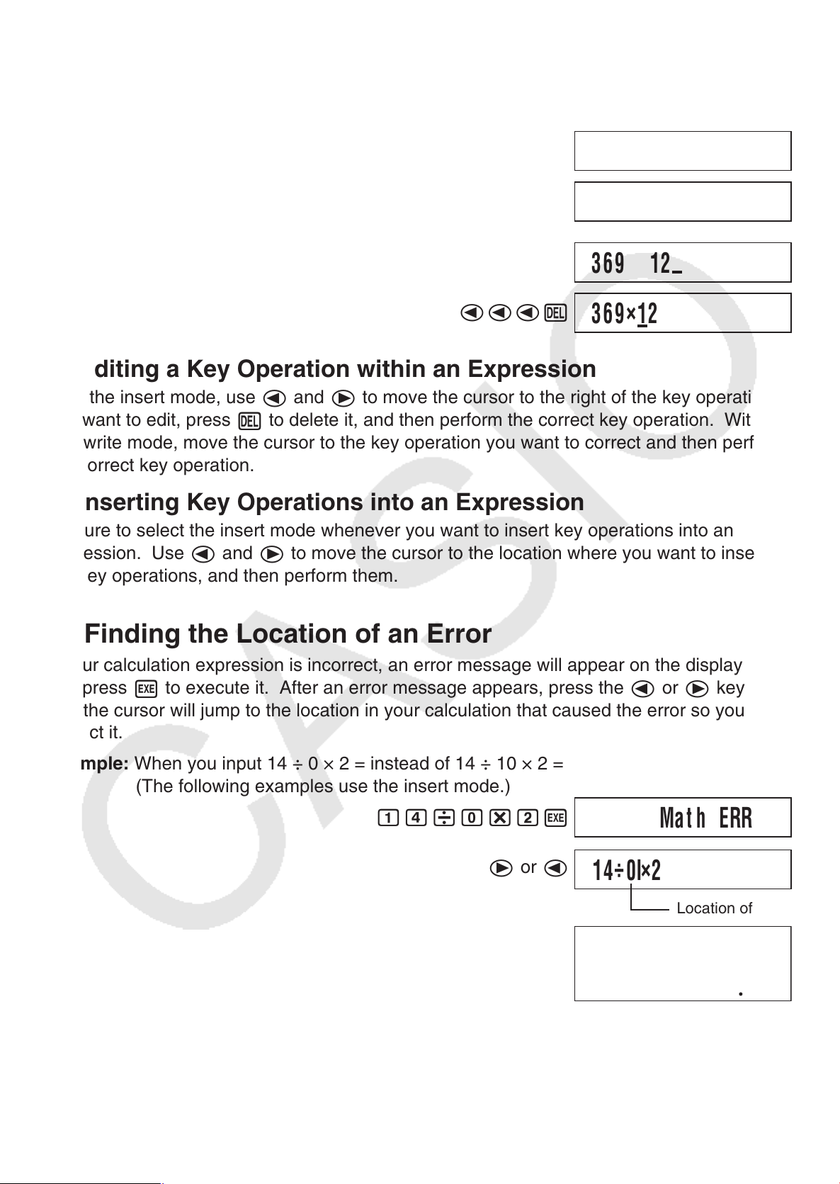
Editing a Key Operation within an Expression

A

With the insert mode, use d and e to move the cursor to the right of the key operation
you want to edit, press D to delete it, and then perform the correct key operation. With the
overwrite mode, move the cursor to the key operation you want to correct and then perform
the correct key operation.

Inserting Key Operations into an Expression

A

Be sure to select the insert mode whenever you want to insert key operations into an
expression. Use d and e to move the cursor to the location where you want to insert
the key operations, and then perform them.

369**12

dddD

369×I12

××

369

12

369×12

Finding the Location of an Error

k

If your calculation expression is incorrect, an error message will appear on the display when
you press w to execute it. After an error message appears, press the d or e key
and the cursor will jump to the location in your calculation that caused the error so you can
correct it.

Example: When you input 14 ÷ 0 × 2 = instead of 14 ÷ 10 × 2 =

(The following examples use the insert mode.)

14/0*2

e

or

w

d

Mat h ERROR

14÷0I×2

Location of Error

14÷10×2

d1w

28

E-10

Basic Calculations

Unless otherwise noted, the calculations in this section can be performed in any of the
calculator’s calculation mode, except for the BASE Mode.

Arithmetic Calculations

k

Arithmetic calculations can be used to perform addition ( +), subtraction ( -),
multiplication ( *), and division ( /).

Example: 7 × 8 − 4 × 5 = 36

7*8-4*5

Fractions

k

Fractions are input using a special separator symbol ( {).

Fraction Calculation Examples

A

2
3

1
4

+

Example 1: 3

Example 2:

Note

• If the total number of elements (integer + numerator + denominator + separator symbols)
of a fraction calculation result is greater than 10 digits, the result will be displayed in
decimal format.

• If an input calculation includes a mixture of fraction and decimal values, the result will be
displayed in decimal format.

• You can input integers only for the elements of a fraction. Inputting non-integers will
produce a decimal format result.

+ 1

1

=

2

2
3

1 1

= 4

1 2

7

(Fraction Display Format: d/c)

6

2$3+1$2

3$1$4+
1$2$3

w

w

w

36

4{11{12

7{6

Switching between Mixed Fraction and Improper Fraction

A

Format

To convert a mixed fraction to an improper fraction (or an improper fraction to a mixed
fraction), press

Switching between Decimal and Fraction Format

A

Press $ to toggle between decimal value and fraction display format.

Note

The calculator cannot switch from decimal to fraction format if the total number of fraction
elements (integer + numerator + denominator + separator symbols) is greater than 10 digits.

!$

(d/c).

E-11

Percent Calculations

k

Inputting a value and with a percent (%) sign makes the value a percent.

Percent Calculation Examples

A

Example 1: 2 % = 0.02 (

2

1 0 0

)

2

!

(

(%)

w

002

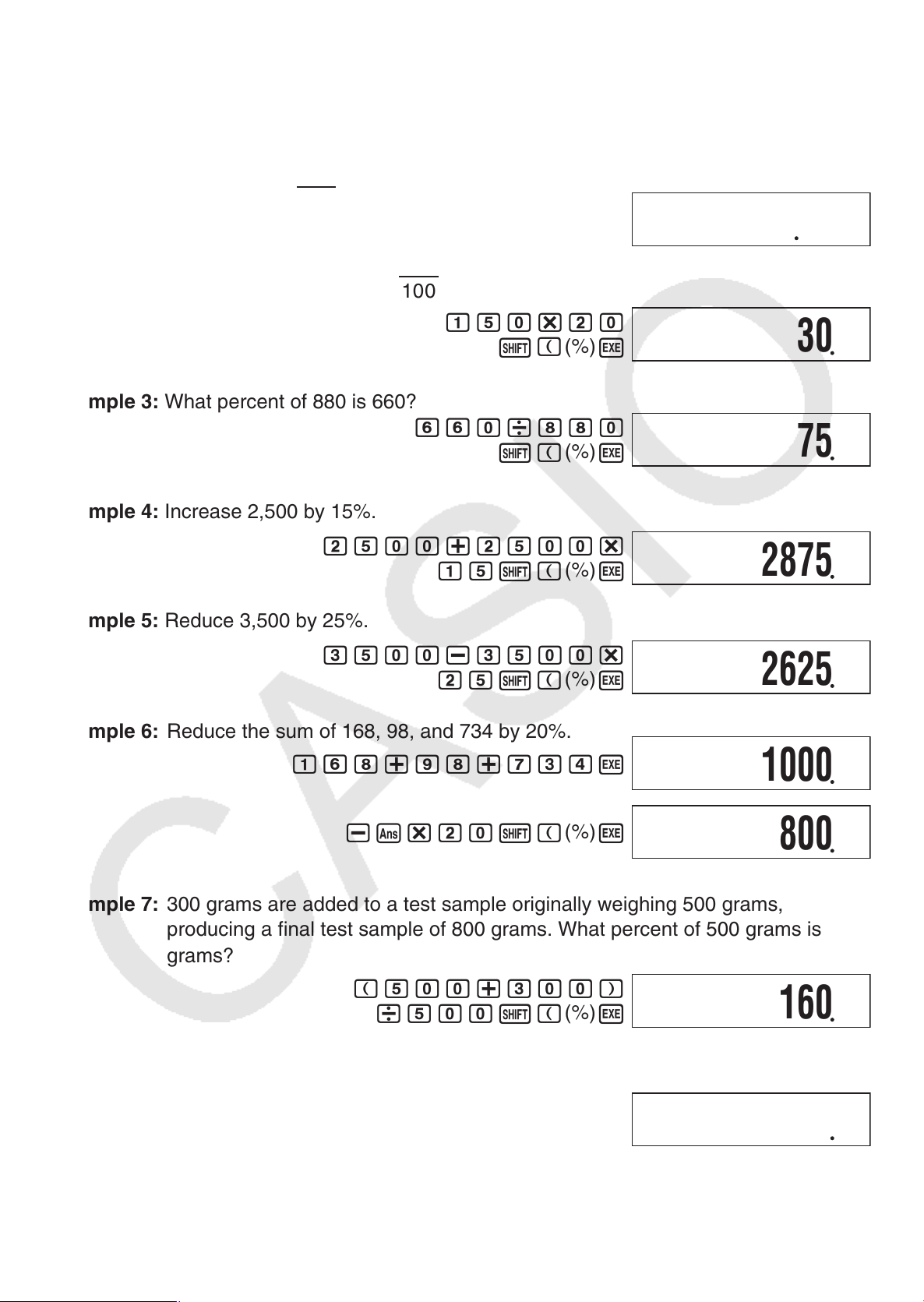
Example 2: 150 × 20% = 30 (150 ×

Example 3: What percent of 880 is 660?

Example 4: Increase 2,500 by 15%.

2500+2500*

Example 5: Reduce 3,500 by 25%.

3500-3500*

20

100

)

150*20

(%)

(

!

660/880

(

!

15

25

!

!

(

(

(%)

(%)

(%)

w

w

w

w

30

75

2875

2625

Example 6: Reduce the sum of 168, 98, and 734 by 20%.

168+98+734

-G*20

Example 7: 300 grams are added to a test sample originally weighing 500 grams,

producing a final test sample of 800 grams. What percent of 500 grams is 800
grams?

(500+300)

/500

Example 8: What is the percentage change when a value is increased from 40 to 46?

(46-40)/40

!

!

!

(

(

(

(%)

(%)

(%)

w

w

w

w

1000
800

160

15

E-12

Degree, Minute, Second (Sexagesimal) Calculations

k

Inputting Sexagesimal Values

A

The following is basic syntax for inputting a sexagesimal value.

{Degrees} $ {Minutes} $ {Seconds}

Example: To input 2°30´30˝

2$30$30

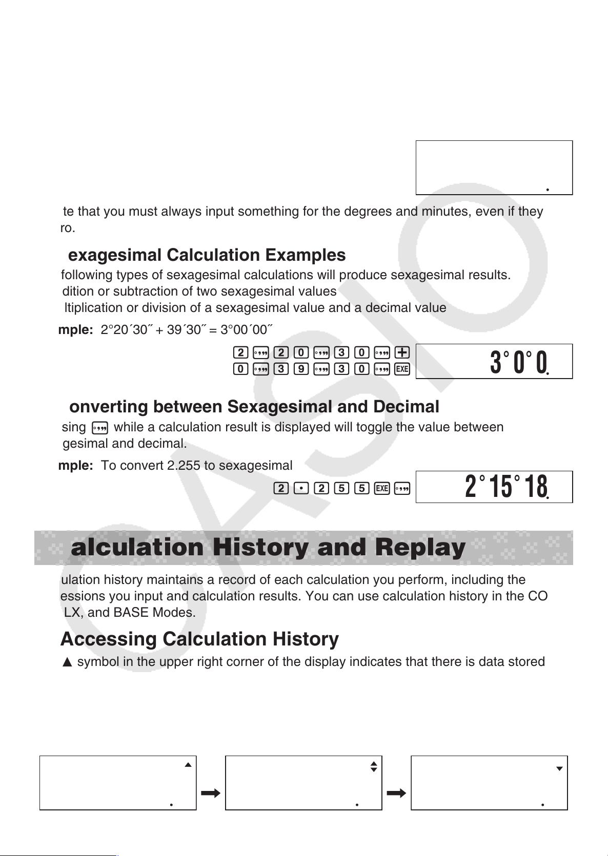
• Note that you must always input something for the degrees and minutes, even if they are
zero.

Sexagesimal Calculation Examples

A

The following types of sexagesimal calculations will produce sexagesimal results.

• Addition or subtraction of two sexagesimal values

• Multiplication or division of a sexagesimal value and a decimal value

Example: 2°20´30˝ + 39´30˝ = 3°00´00˝

2$20$30$+
0$39$30

Converting between Sexagesimal and Decimal

A

$

$w

$w

2˚30˚30

2˚30˚30

˚

3˚0˚0

Pressing $ while a calculation result is displayed will toggle the value between
sexagesimal and decimal.

Example: To convert 2.255 to sexagesimal

2.255

w$

2˚15˚18

Calculation History and Replay

Calculation history maintains a record of each calculation you perform, including the
expressions you input and calculation results. You can use calculation history in the COMP,
CMPLX, and BASE Modes.

Accessing Calculation History

k

The ` symbol in the upper right corner of the display indicates that there is data stored in
calculation history. To view the data in calculation history, press f. Each press of f
will scroll upwards (back) one calculation, displaying both the calculation expression and its

result.

Example:

3+3

1+1w2+2w3+3

ff

2+2

6

E-13

w

4

1+1

2

While scrolling through calculation history records, the $ symbol will appear on the display,
which indicates that there are records below (newer than) the current one. When this
symbol is turned on, press c to scroll downwards (forward) through calculation history
records.

Important!

• Calculation history records are all cleared whenever you press p, when you change to a
different calculation mode, and whenever you perform any reset operation.

• Calculation history capacity is limited. Whenever you perform a new calculation while
calculation history is full, the oldest record in calculation history is deleted automatically to
make room for the new one.

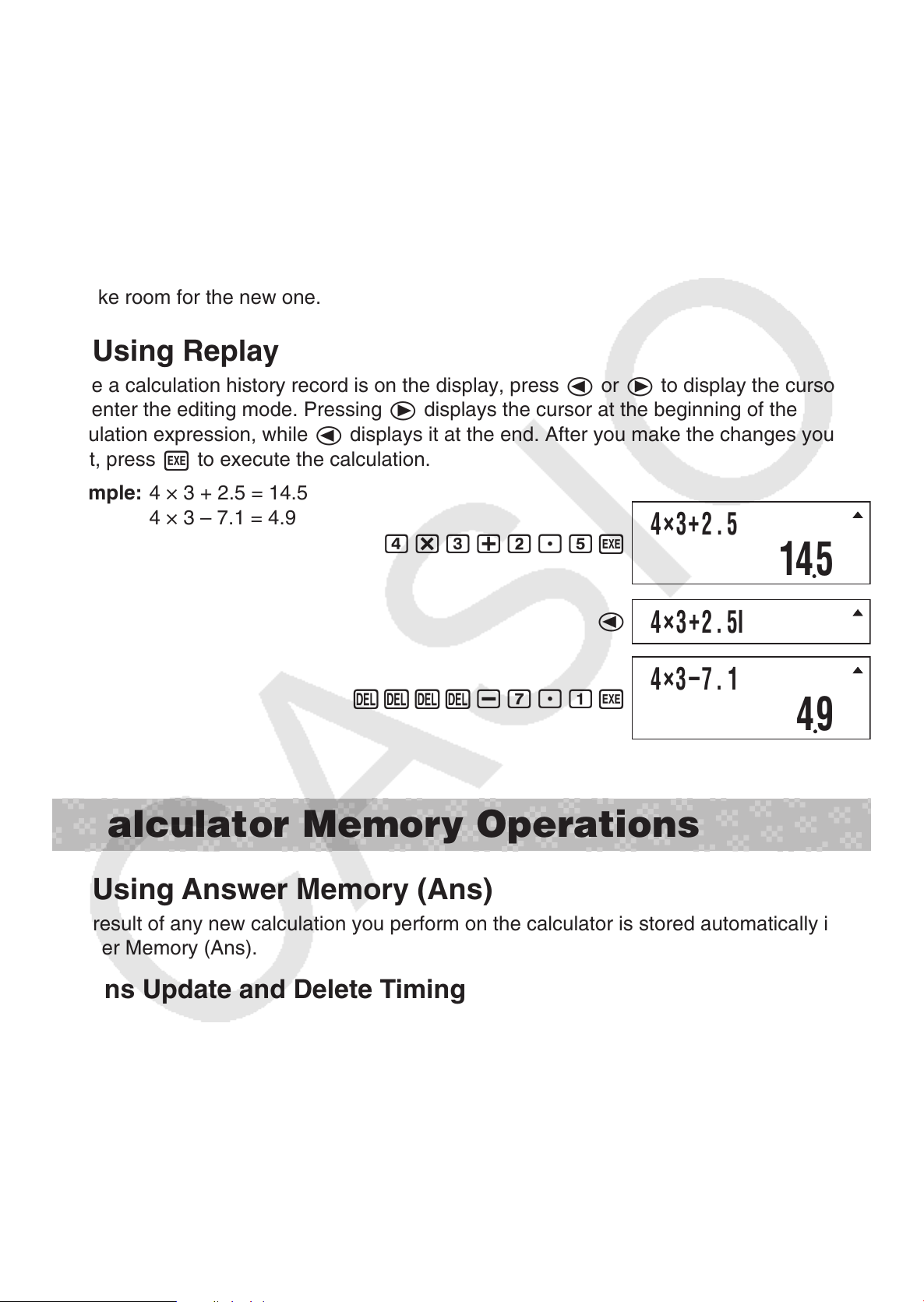
Using Replay

k

While a calculation history record is on the display, press d or e to display the cursor
and enter the editing mode. Pressing e displays the cursor at the beginning of the
calculation expression, while d displays it at the end. After you make the changes you
want, press w to execute the calculation.

Example: 4 × 3 + 2.5 = 14.5

4 × 3 – 7.1 = 4.9

4*3+2.5

w

4×3+2.5

145

d

4×3+2.5I

4×3–7.1

DDDD

-7.1

w

49

Calculator Memory Operations

Using Answer Memory (Ans)

k

The result of any new calculation you perform on the calculator is stored automatically in
Answer Memory (Ans).

Ans Update and Delete Timing

A

When using Ans in a calculation, it is important to keep in mind how and when its contents
change. Note the following points.

• The contents of Ans are replaced whenever you perform any of the following operations:
calculate a calculation result, add a value to or subtract a value from independent
memory, assign a value to a variable or recall the value of a variable, or input statistical
data in the SD Mode or REG Mode.

• In the case of a calculation that produces more than one result (like coordinate
calculations), the value that appears first on the display is stored in Ans.

• The contents of Ans do not change if the current calculation produces an error.

E-14

• When you perform a complex number calculation in the CMPLX Mode, both the real part
and the imaginary part of the result are stored in Ans. Note, however, that the imaginary
part of the value is cleared if you change to another calculation mode.

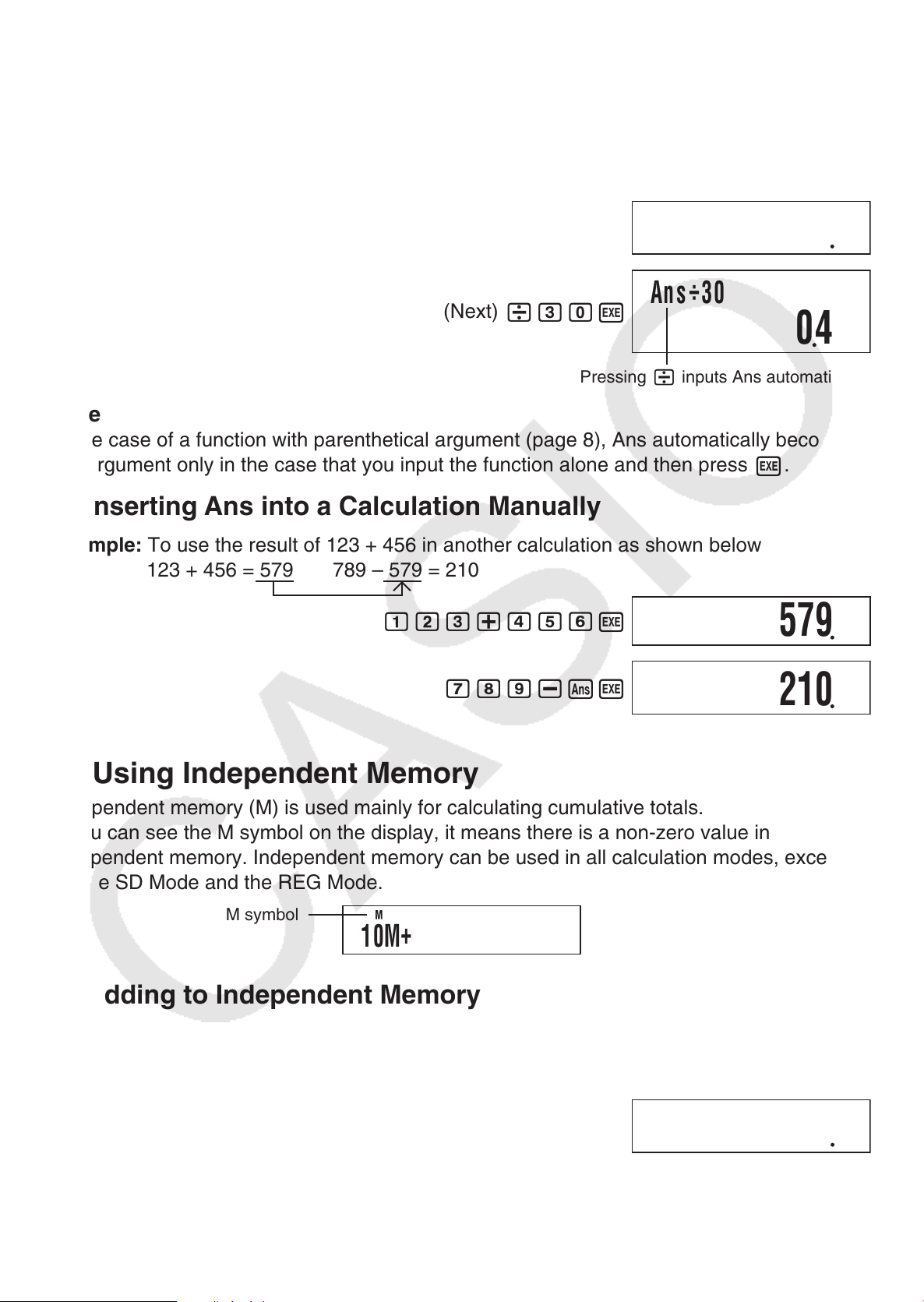
Automatic Insertion of Ans in Consecutive Calculations

A

Example: To divide the result of 3 × 4 by 30

3*4

(Next)

Note

In the case of a function with parenthetical argument (page 8), Ans automatically becomes
the argument only in the case that you input the function alone and then press w.

Inserting Ans into a Calculation Manually

A

Example: To use the result of 123 + 456 in another calculation as shown below

123 + 456 = 579 789 – 579 = 210

123+456

/30

w

12

Ans÷30

w

04

Pressing / inputs Ans automatically.

w

579

789-

Using Independent Memory

k

Independent memory (M) is used mainly for calculating cumulative totals.
If you can see the M symbol on the display, it means there is a non-zero value in
independent memory. Independent memory can be used in all calculation modes, except
for the SD Mode and the REG Mode.

M symbol

+

Adding to Independent Memory

A

While a value you input or the result of a calculation is on the display, press m to add it to
independent memory (M).

Example: To add the result of 105 ÷ 3 to independent memory (M)

10M

105/3

Kw

m

210

35

E-15

Subtracting from Independent Memory

A

While a value you input or the result of a calculation is on the display, press
subtract it from independent memory (M).

Example: To subtract the result of 3 × 2 from independent memory (M)

3*2

Note

Pressing m or
subtract it from independent memory.

Important!

The value that appears on the display when you press m or
calculation in place of w is the result of the calculation (which is added to or subtracted
from independent memory). It is not the current contents of independent memory.

Viewing Independent Memory Contents

A

Press

A

tm

Clearing Independent Memory Contents (to 0)

1m

(M).

(M–) while a calculation result is on the display will add it to or

1m

(M–)

1m

(M–) at the end of a

1m

(M–) to

6

0

1t

Clearing independent memory will cause the M symbol to turn off.

Using Variables

k

The calculator supports six variables named A, B, C, D, X, and Y, which you can use to
store values as required. Variables can be used in all calculation modes.

Assigning a Value or Calculation Result to a Variable

A

Use the procedure shown below to assign a value or a calculation expression to a variable.

Example: To assign 3 + 5 to variable A

Viewing the Value Assigned to a Variable

A

To view the value assigned to a variable, press t and then specify the variable name.

Example: To view the value assigned to variable A

Using a Variable in a Calculation

A

You can use variables in calculations the same way you use values.

(STO)

m

(M)

3+5

1t

-

t

(STO)-(A)

(A)

Example: To calculate 5 + A

Clearing the Value Assigned to a Variable (to 0)

A

Example: To clear variable A

5+

0

1t

a-

(A)

w

(STO)-(A)

E-16

Clearing All Memory Contents

k

Perform the following key operation when you want to clear the contents of independent
memory, variable memory, and Answer Memory.

(CLR)1(Mem)

9

1

w

• If you do not want to clear the calculator’s settings, press A in place of
operation.

in the above

w

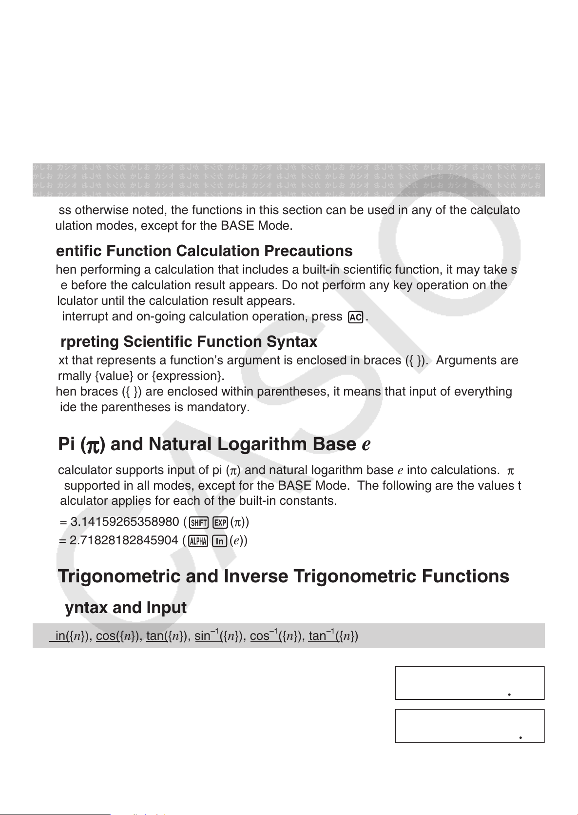
Scientific Function Calculations

Unless otherwise noted, the functions in this section can be used in any of the calculator’s
calculation modes, except for the BASE Mode.

Scientific Function Calculation Precautions

• When performing a calculation that includes a built-in scientific function, it may take some
time before the calculation result appears. Do not perform any key operation on the
calculator until the calculation result appears.

• To interrupt and on-going calculation operation, press A.

Interpreting Scientific Function Syntax

• Text that represents a function’s argument is enclosed in braces ({ }). Arguments are
normally {value} or {expression}.

• When braces ({ }) are enclosed within parentheses, it means that input of everything
inside the parentheses is mandatory.

Pi (π) and Natural Logarithm Base

k

The calculator supports input of pi (π) and natural logarithm base e into calculations. π and

e

are supported in all modes, except for the BASE Mode. The following are the values that

the calculator applies for each of the built-in constants.

= 3.14159265358980 (

π

e

= 2.71828182845904 (

Trigonometric and Inverse Trigonometric Functions

k

Syntax and Input

A

sin( { n }), cos( { n }), tan( { n }), sin

Example: sin 30 = 0.5, sin

1e

Si

–1

0.5 = 30 (Angle Unit: Deg)

(π))

(e))

–1

({ n }), cos

1s

–1

({ n }), tan

–1

)

(sin

–1

30)

s

0.5)

({ n })

e

w

w

05
30

E-17

Notes

A

• These functions can be used in the CMPLX Mode, as long as a complex number is not
used in the argument. A calculation like

is not.

• The angle unit you need to use in a calculation is the one that is currently selected as the
default angle unit.

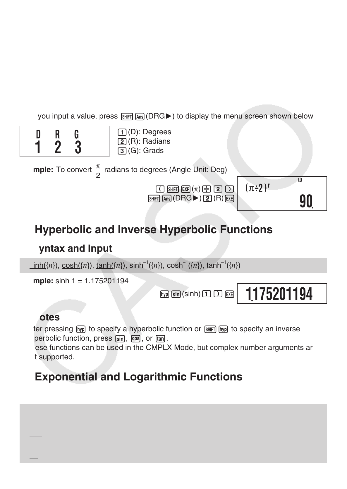
Angle Unit Conversion

k

You can convert a value that was input using one angle unit to another angle unit.
After you input a value, press

1(D): Degrees

DRG

Example: To convert

312

π

radians to degrees (Angle Unit: Deg)

2

1G

( R ): Radians

2

( G ): Grads

3

(DRG ') to display the menu screen shown below.

1G

× sin(30) is supported for example, but sin(1 +

i

(

(

)

π

1e

(DRG ') 2( R )

/2)

E

(

π

÷

2

r

)

90

)

i

Hyperbolic and Inverse Hyperbolic Functions

k

Syntax and Input

A

sinh({ n }), cosh( { n }), tanh( { n }), sinh

Example: sinh 1 = 1.175201194

Notes

A

• After pressing w to specify a hyperbolic function or
hyperbolic function, press s, c, or t.

• These functions can be used in the CMPLX Mode, but complex number arguments are
not supported.

Exponential and Logarithmic Functions

k

–1

({ n }), cosh

w

s

–1

({ n }), tanh

(sinh)

1)

1w

–1

({ n })

E

1175201194

to specify an inverse

Syntax and Input

A

10^( { n }) .......................... 10

e

^({ n }) .............................

log( { n }) ........................... log

m

log( {
ln( {

},{ n }) ..................... log

n

}) ............................. log e { n } (Natural Logarithm)

{

}

n

{

}

n

e

{ n } (Common Logarithm)

10

{ n } (Base { m } Logarithm)

{

}

m

E-18