How it Works
Log In / Sign Up
Buy Points
How it Works
FAQ
Contact Us
Questions and Suggestions
Users
CASIO
Loading...
C
Celviano AP-25
2
Celviano AP-28
2
CELVIANO AP-31
2
CELVIANO AP-33
2
CELVIANO AP-38
Celviano AP-40
CELVIANO AP-420
3
Celviano AP-420BN
Celviano AP-45
2
Celviano AP-470BK
2
Celviano AP-470BN
2
Celviano AP-470WE
2
CELVIANO AP-500
3
CELVIANO AP-6
Celviano AP-60R
Celviano AP-65R
celviano ap-700
Celviano AP-710
CELVIANO AP-80R
2
Celviano GP-300
Celviano GP-300BK
Celviano GP-310BK
Celviano GP-310WE
Celviano GP-500
Celviano GP-510BP
2
CFX-9800G
5
CFX-9800G-w
CFX-9800G-w - Color Graphing Calculator
CFX-9850G
4
CFX9850GB
4
CFX-9850GB PLUS
11
CFX-9850GC plus
4
CFX-9850G PLUS
28
CFX-9900GC
CFX-9940GT
CFX-9950G
CFX9950GB
2
CFX-9950GB PLUS
6
CFX9970G
26
CGP-700
2
CHF-100-1V
CHR-100-1
CHR200-1
ClassPad 101
ClassPad300
9
ClassPad300PLUS
5
ClassPad 330
8
CLASSPAD 330 3.04
CLASSPAD 330 PLUS
4
CLASSPAD II
ClassPad II fx-CP400+E
ClassPad Manager
2
ClassPad UNITS 3 4
ClassWiz fx-991EX
CLOCK (SNZ) B
Collection AMW-700B-1AVEF
COMBIWAVE1
COMBIWVGE1
2
COMMANDO GzOne
CompactWLAN
Cosmo CZ-1
Cosmo CZ-230S
Cosmo CZ-5000
Cosmosunthesizer CZ-3000
cp-10
CP-1260
CP-2070
CP-725
CPS130
CPS-7
3
CPS-85
CQ-1
3
CQ 2
CR-200S
CS-2X
CS-410P
CS-43P
CS-44
CS-44 P
2
CS-4B
CS-53P
CS-55P
CS-65P
2
CS-66P
2
CS-67P
CS-67PWE
CS-68PBK
CS-7W
CSF-4450
2
CSF-4450A
2
CSF-4650
2
CSF-4650A
3
CSF-4950
2
CSF-4950A
3
CSF-4970A
3
CSF-5350
2
CSF-5550
2
CSF-5750
2
CSF-7950
3
CSF-8950
3
Loading...
Loading...
Nothing found
ClassPad UNITS 3 4
User Manual
11 pgs
666.02 Kb
1
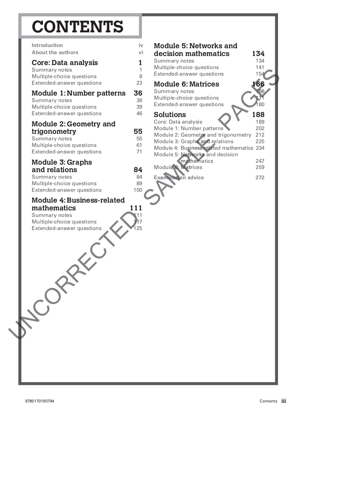
Table of contents
Loading...
CASIO ClassPad UNITS 3 4 User Manual
...
CASIO User Manual
Download
Specifications and Main Features
Frequently Asked Questions
User Manual
Download
Page 1
Page 2
Page 3
Page 4
Page 5
Page 6
Page 7
Page 8
Page 9
Page 10
Page 11
Loading...
+
hidden pages
Unhide
You need points to download manuals.
1 point = 1 manual.
You can buy points or you can get point for every manual you upload.
Buy points
Upload your manuals
 Loading...