

Page 1

Manual | EN
TE1510
TwinCAT 3 | CAM Design Tool
2020-10-09 | Version: 1.1
Page 2

Page 3

Table of contents
Table of contents
1 Foreword ....................................................................................................................................................5
1.1 Notes on the documentation..............................................................................................................5
1.2 Safety instructions .............................................................................................................................6
2 Introduction................................................................................................................................................7
3 Licensing..................................................................................................................................................13
4 The Properties of the Master ..................................................................................................................14
5 The Properties of the Slave ....................................................................................................................16
6 Graphic Window ......................................................................................................................................18
7 Tables Window.........................................................................................................................................20
8 Commands ...............................................................................................................................................23
9 Examples..................................................................................................................................................26
9.1 Overview..........................................................................................................................................26
9.2 Example 1........................................................................................................................................26
9.3 Example 2........................................................................................................................................28
9.4 Example 3........................................................................................................................................29
9.5 Example 4........................................................................................................................................31
9.6 Example 5........................................................................................................................................33
9.7 Example 6........................................................................................................................................36
9.8 Example 7........................................................................................................................................38
TE1510 3Version: 1.1
Page 4

Table of contents
TE15104 Version: 1.1
Page 5

Foreword
1 Foreword
1.1 Notes on the documentation
This description is only intended for the use of trained specialists in control and automation engineering who
are familiar with applicable national standards.
It is essential that the documentation and the following notes and explanations are followed when installing
and commissioning the components.
It is the duty of the technical personnel to use the documentation published at the respective time of each
installation and commissioning.
The responsible staff must ensure that the application or use of the products described satisfy all the
requirements for safety, including all the relevant laws, regulations, guidelines and standards.
Disclaimer
The documentation has been prepared with care. The products described are, however, constantly under
development.
We reserve the right to revise and change the documentation at any time and without prior announcement.
No claims for the modification of products that have already been supplied may be made on the basis of the
data, diagrams and descriptions in this documentation.
Trademarks
Beckhoff®, TwinCAT®, EtherCAT®, EtherCAT G®, EtherCAT G10®, EtherCAT P®, Safety over EtherCAT®,
TwinSAFE®, XFC®, XTS® and XPlanar® are registered trademarks of and licensed by Beckhoff Automation
GmbH.
Other designations used in this publication may be trademarks whose use by third parties for their own
purposes could violate the rights of the owners.
Patent Pending
The EtherCAT Technology is covered, including but not limited to the following patent applications and
patents:
EP1590927, EP1789857, EP1456722, EP2137893, DE102015105702
with corresponding applications or registrations in various other countries.
EtherCAT® is a registered trademark and patented technology, licensed by Beckhoff Automation GmbH,
Germany
Copyright
© Beckhoff Automation GmbH & Co. KG, Germany.
The reproduction, distribution and utilization of this document as well as the communication of its contents to
others without express authorization are prohibited.
Offenders will be held liable for the payment of damages. All rights reserved in the event of the grant of a
patent, utility model or design.
TE1510 5Version: 1.1
Page 6
Foreword
1.2 Safety instructions
Safety regulations
Please note the following safety instructions and explanations!
Product-specific safety instructions can be found on following pages or in the areas mounting, wiring,
commissioning etc.
Exclusion of liability
All the components are supplied in particular hardware and software configurations appropriate for the
application. Modifications to hardware or software configurations other than those described in the
documentation are not permitted, and nullify the liability of Beckhoff Automation GmbH & Co. KG.
Personnel qualification
This description is only intended for trained specialists in control, automation and drive engineering who are
familiar with the applicable national standards.
Description of symbols
In this documentation the following symbols are used with an accompanying safety instruction or note. The
safety instructions must be read carefully and followed without fail!
DANGER
Serious risk of injury!
Failure to follow the safety instructions associated with this symbol directly endangers the life and health of
persons.
WARNING
Risk of injury!
Failure to follow the safety instructions associated with this symbol endangers the life and health of persons.
CAUTION
Personal injuries!
Failure to follow the safety instructions associated with this symbol can lead to injuries to persons.
NOTE
Damage to the environment or devices
Failure to follow the instructions associated with this symbol can lead to damage to the environment or
equipment.
Tip or pointer
This symbol indicates information that contributes to better understanding.
TE15106 Version: 1.1
Page 7

Introduction
2 Introduction
A cam plate editor is used to design the motions for a cam plate.
The cam plate editor is a flexible tool that provides optimum user support. The responsibility for the choice of
parameters lies with you (the user). You should check carefully whether the start and end points meet the
specification. The graphic display options provide optimum support for controlling velocities, accelerations
and jerk.
Notwithstanding the wide range of options, please bear in mind the limits to possible motions imposed by
physical constraints.
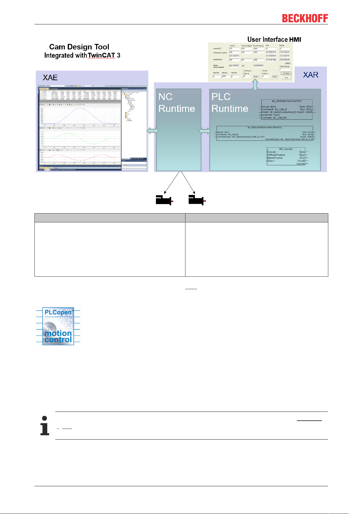
The CAM Design Tool is the cam plate editor of TwinCAT. It is integrated into the XAE engineering
environment based on Visual Studio™. In the user interface it can be found under the System Manager
(see diagram).
Cam plates that have been designed with the tool are stored in the respective project file. When the system
is started, the cam plates are automatically transferred to the eXtended Automation Runtime (XAR).
eXtended Automation (XA) architecture
In XAR, the NC includes the functionalities required for coupling cam plates. These extensive functionalities
can be called by the PLC with the TC-NC Camming library (TF5050). In addition to the standard function
blocks of PLC Open, the library also contains compatible function blocks with extended functionalities. The
following overview illustrates the options available through interaction of the CAM Design Tool with the NC
and the PLC.
It is also possible, for example, to upload cam plates generated by the PLC, which were loaded into the NC
via a function block, into the CAM Design Tool.
A user interface (HMI) can be connected via the PLC.
TE1510 7Version: 1.1
Page 8
Introduction
Generate CAM offline: CAM Design Tool Generate CAM online: PLC Code
Engineering: For designing a cam plate.
• Motions are defined segment by segment.
• The position, velocity and acceleration can be
checked.
Information about the TF5050 PLC library can be found here.
PLC open Motion Control
The function blocks listed in the PLC library are based on:
Technical Specification
• PLCopen - Technical Committee 2 - Task Force
• Function blocks for motion control
PLC: For use in the production machine.
• A touch probe option is available.
• The format can be changed via the HMI.
• Facilitates checking of characteristic values, if
required.
Create project
A license is required to access the full functionality of the TE1510 CAM Design Tool, see Licensing
[}13].
The cam plate editor integrated in TwinCAT 3 can be found in a Twin CAT project under MOTION > Tables.
TE15108 Version: 1.1
Page 9
Introduction
Here you can insert additional Masters and below that corresponding Slaves by right-clicking.
Click the Master in the structure tree to open the property pages. Not only the properties of the Master
[}14] but also those of the associated Slaves [}16] can be set on these pages.
TE1510 9Version: 1.1
Page 10
Introduction
The general procedure for designing a cam plate is based on VDI Guideline 2143. The rough design of the
motion - the motion plan - defines the start and end points of the motion section. However, the cam plate
editor does not differentiate between the motion sketch and the motion diagram containing the detailed
motion description.
TE151010 Version: 1.1
Page 11
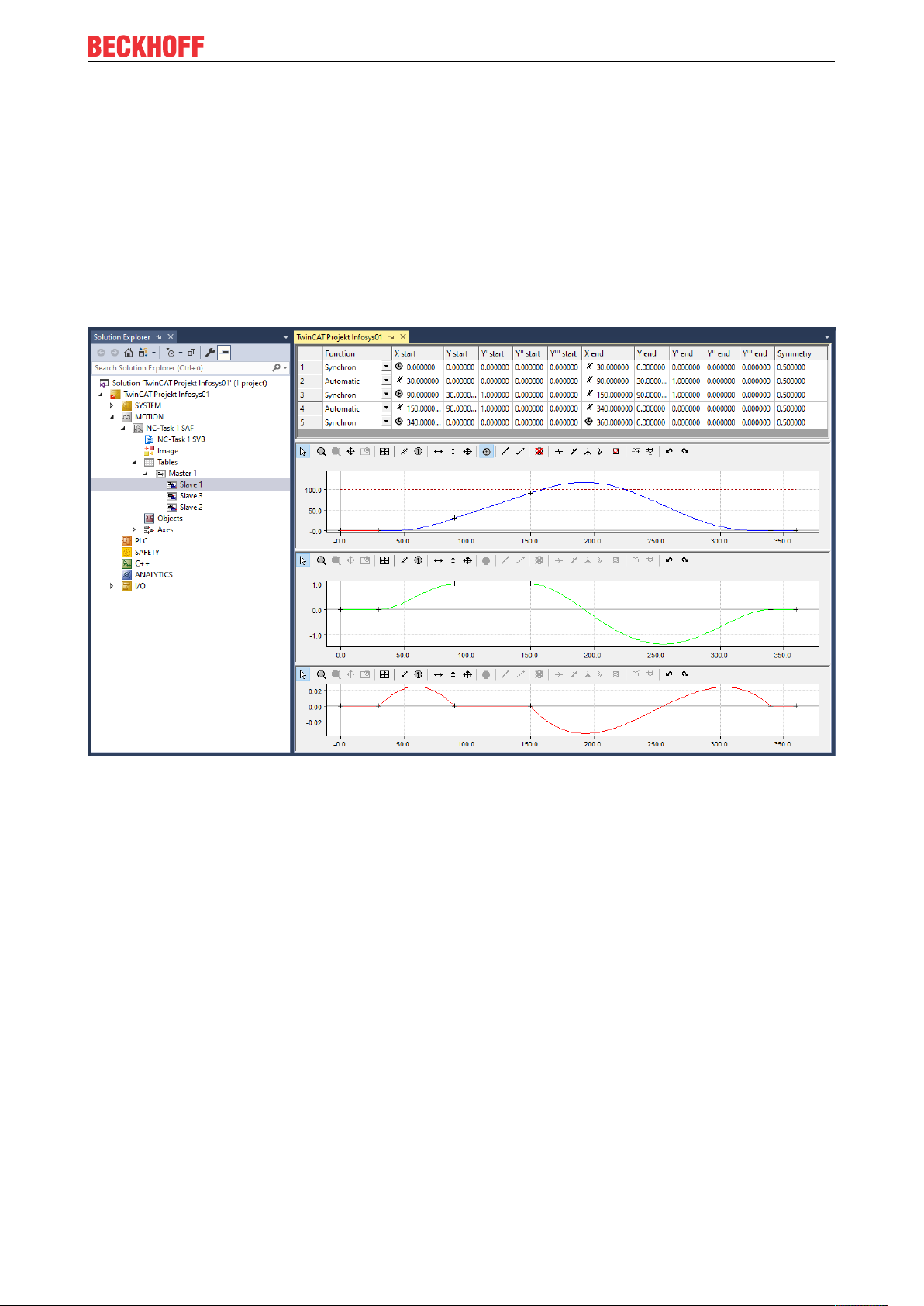
Introduction
The user's interface to the cam plate editor is largely graphic. Following interactive graphic entry of the points
in the graphic window, the co-ordinates of the points are displayed in the table window above it.
New points can only be inserted in the graph, and it is only possible to delete existing points via the graph.
The properties of the points - the co-ordinate values or their derivatives - can also be interactively
manipulated in the table window.
The following parameters can be displayed in the graphical area:
• position,
• velocity,
• acceleration,
• jerk.
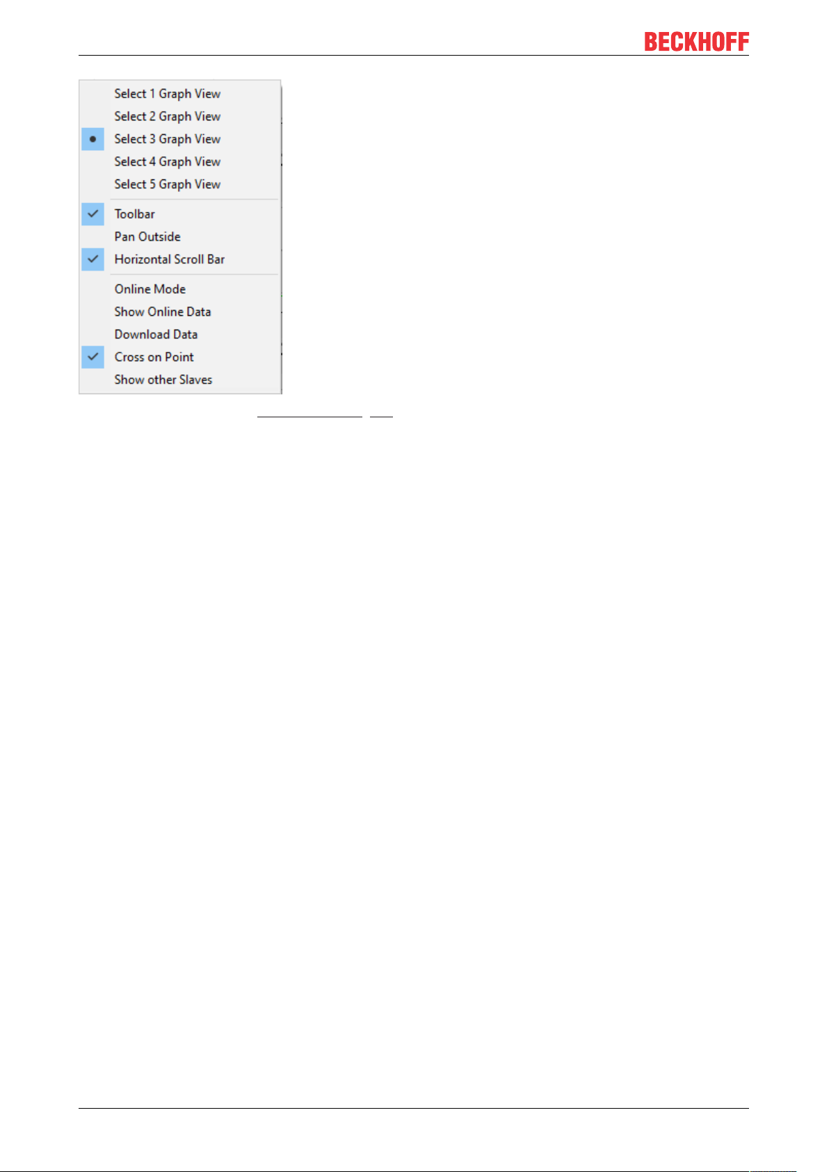
Change display
ü The mouse pointer is in the graphic window.
1. Right-click.
2. Select the desired views in the menu window.
TE1510 11Version: 1.1
Page 12
Introduction
ð For example, a separate graphic window [}18] is created for each derivative.
TE151012 Version: 1.1
Page 13
Licensing
3 Licensing
The functionality of the CAM Design Tool is included in the XAE of TwinCAT, which means there is no need
to download an additional software module. A license is required to save a cam plate in a project file. See
"Ordering and activation of TwinCAT 3 standard licenses".
Once a cam plate has been created in a project it cannot be changed, but it remains in the project. A license
is only required on the workstations on which cam plates are designed or modified.
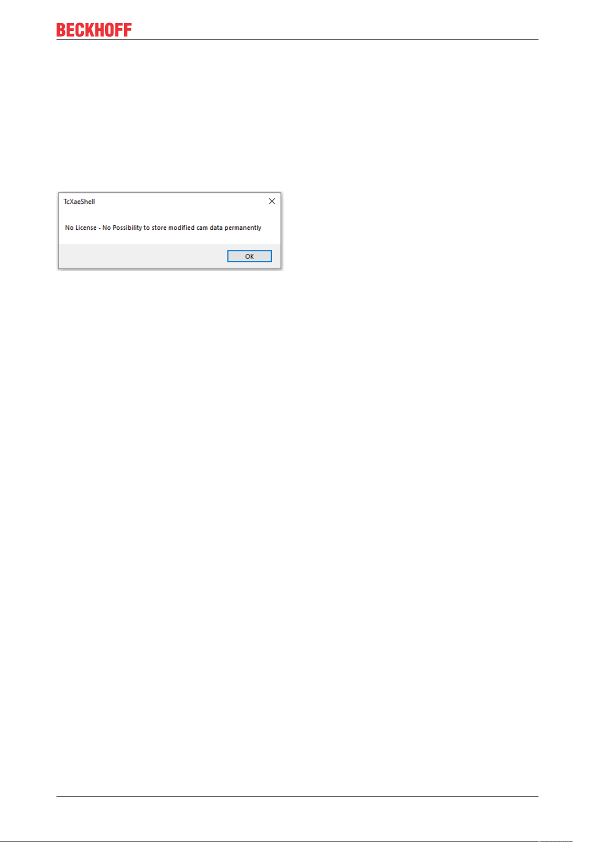
If no license is available at the workstation, a message is displayed the first time a new cam plate is created,
which the user must confirm:
Required licenses:
TE1510 CAM Design Tool
Although this license must be activated on the target system, it is an engineering license. For testing
purposes, a demo mode simulation can be used without a license.
Restrictions in the demo version
Cam plates generated without a license can be loaded into the XAR. However, they are ignored when the
project is saved.
TE1510 13Version: 1.1
Page 14

The Properties of the Master
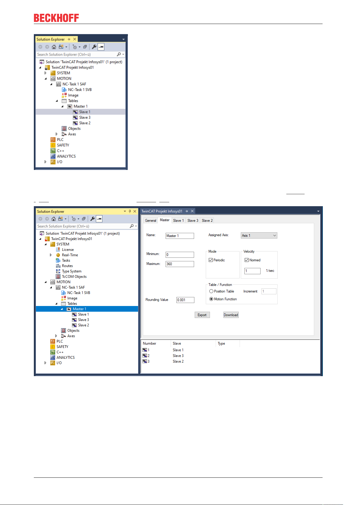
4 The Properties of the Master
On the property page of the master, the minimum and maximum of the master position can be set.
Velocity
The Normed checkbox can be used to choose between the normalized display and a physical display that
shows the velocities, accelerations and jerk of the slaves as a function of time. The normalized display refers
these displays to the master position.
Mode
For the physical representation the velocity of the master is required. First, a distinction is made between a
linear axis and a rotary axis (values are given as angles in degrees). The choice between linear and rotary
axis determines the table type – linear or cyclic – for transferring the data to the numerical control (NC).
For a rotary Master, the first and second derivatives at the end are set equal to the corresponding figures at
the start of the motion cycle, if the start and end positions of the slave correspond to the minimum and
maximum positions of the master.
Table/Function
The Position table function is used to select the tables with the table values (master value, slave value) at a
defined distance from the master values (increment).
The Increment function defines the increment of the master position for outputting the tables to a file. If an
equidistant table is to be generated, the total length (the actual maximum minus the minimum) should be
divisible by the increment. When the configuration is activated, the information for creating and transferring
the tables with this increment to the NC is generated automatically.
Motion Function can be used to transfer the complete slave information to the NC. This means that only the
edge points of the segments and the corresponding information, such as the law of motion, are loaded into
the NC. The NC then calculates the corresponding slave values (position, velocity and acceleration) for the
current master position during runtime. Past problems that had their origin in the discretization of the data in
the table essentially no longer exist.
TE151014 Version: 1.1
Page 15

The Properties of the Master
Functionalities such as special motion laws that are not yet available in the NC are marked in red in
the cam plate editor. These may not be selected.
The Rounding Value rounds the master position in the graphic input with the given value.
Importing slaves
• Right-click the master in the tree view and select the Add existing element.
Saving and exporting slaves
1. Right-click the slave in the tree view and select Save slave 1 as.
2. Save the file as an export file (*.xti).
ð The data can be imported via the tree view under Master.
TE1510 15Version: 1.1
Page 16

The Properties of the Slave
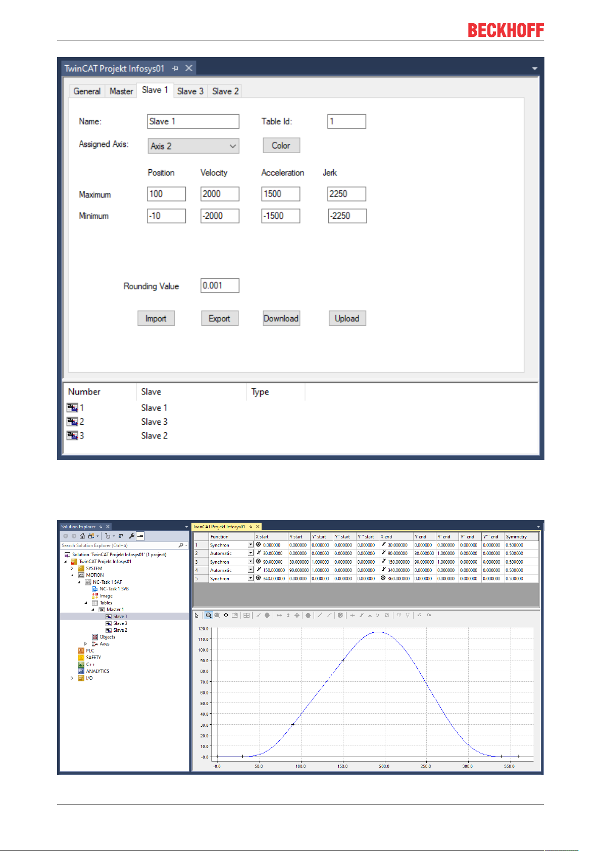
5 The Properties of the Slave
Settings on the property page of the slave
• Maximum and minimum position,
• Velocity,
• Acceleration,
• Jerk.
These values can be used as initial specifications when the graphic window is first displayed.
The current values in the diagram can be adjusted in the respective graphic window with the command
Adjust extreme values .
TE151016 Version: 1.1
Page 17

The Properties of the Slave
Button/Input Description
Rounding value Rounds the slave positions in the graphical input with the specified value.
Export The Export button can be used to store the slave values in a line in an ASCII file in
the form master and slave position. The master position increment is specified in the
master's property page.
Import The Import button can be used to import files in the form just described. The values
can then be displayed as cubic splines. The type of the spline still needs to be
adjusted in the table, according to the values.
Download The Download button can be used to transfer the current data to the NC, as long as
the slave is not coupled, since the tables are deleted completely and refilled with
data.
Upload The Upload button can be used to upload the function information from the NC.
Existing data are deleted entirely, and the NC data can be manipulated in the table
as well as in the graphic.
Table ID The Table Id provides a unique identifying number (1-4095) for the table, with the aid
of which the table data is stored in the NC.
When uploading cyclic data, the period length of the master must match that of the loaded data.
The master can be set to linear (non-cyclic) for direct data checking.
Table ID
The table ID can be changed by right-clicking the slave in the tree view and selecting the command Change
ID.
The option Save Slave... can be used to save the motion diagram data in an export file (*.xti). This data can
be imported again under a master.
TE1510 17Version: 1.1
Page 18

Graphic Window
6 Graphic Window
The slave's position and derivatives are each shown in separate graphic windows.
Toolbar
The toolbar of the graphic window contains buttons that only refer to the diagram:
as well as the special commands for the cam plate editor:
The graphic commands are divided into:
• Input mode:
There are also zoom and move commands:
• Zoom
• Zoom all
• Move: This command only becomes active when the zoom command has been called.
If you activate the menu item Pan Outside, you can move across boundaries.
Pan Outside can be activated via the menu of the graphic window by right-clicking.
Overview window on/off
The window can only be enabled via the button if you have zoomed into the window.
If the overview window is activated, the window not only shows which section the graphic is in, you can
also move the section or zoom into a new section.
TE151018 Version: 1.1
Page 19

Graphic Window
The horizontal and vertical scrollbars allow you to move the graphic section. The horizontal scrollbar
applies to all graphic windows simultaneously.
If you use an IntelliMouse with a scroll wheel, you can zoom using the scroll wheel.
Show/hide toolbar
The toolbar containing the commands can be shown or hidden by right-clicking (in the graphic window) the
following menu:
If the Horizontal scrollbar option is enabled, a horizontal scrollbar is available for this window. All horizontal
scrollbars are synchronized.
The Cross on Point option causes the start and end points of motion sections to be indicated by a cross.
The Show online data option displays the table data currently in the NC with the corresponding table ID as
a cubic spline. Currently this can result in a distorted display, because the linear tables are displayed as
natural splines (second derivative at the edges equals null). The data is displayed in the same color, but
somewhat darker.
The data is automatically transferred by ADS, as soon as Online Mode is switched on. The current data can
be read by switching the mode on and off.
When the configuration is activated, the information for creating and transferring the tables to the NC is
generated automatically.
Use Download data to transfer the data to the NC. In this case the restriction applies that the slave is not
coupled for the function (see slave properties [}16]). In other words, only the data is transferred.
TE1510 19Version: 1.1
Page 20

Tables Window
7 Tables Window
The values for the motion section are displayed in the table window:
Table header Description
Function Indicates the function type (see function types).
X start Initial value of the master position.
(The icon in front of the value indicates the type of the point.)
Y start Initial value of the slave position.
Y' start Initial value of the slave velocity.
Y'' start Initial value of the slave acceleration.
Y''' start Start value of the slave jerk.
X end End value of the master position.
(The icon in front of the value indicates the type of the point.)
Y end End value of the slave position.
Y' end End value of the slave velocity.
Y'' end End value of the slave acceleration.
Y''' end End value of the slave jerk.
Symmetry Symmetry value of the law of motion.
You can change the values using the keyboard.
The restrictions imposed by the choice of the function type or the boundary conditions for the points are
taken into account.
Since motion sections are normally contiguous - except for Slide Points - the end point and its derivatives at
the end of the section is equal to the corresponding values at the start of the following motion section.
Therefore, you should normally always manipulate the initial values.
In addition, if you find any discrepancies in a finished motion diagram, check that the start and end points
match.
If certain values in the table cannot be changed, you should reconsider the boundary conditions of the points
and change them if necessary.
The boundary conditions limit the scope of the functions in sections in accordance with their type.
The symmetry of the functions can only be changed for the following types:
• Polynomial3,
• Polynomial5,
• Polynomial8,
• Sineline,
• ModSineline,
• Bestehorn,
• AccTrapezoid.
Normally the inflection on the curve (acceleration = 0) at 50 % = 0.5.
This value can be modified not only in the table, but also in the graph (see Example 6 [}36]).
TE151020 Version: 1.1
Page 21

Tables Window
Function Types
In addition to the standard types (synchronous/automatic), which can be changed by command on the graph,
the function type can also be modified in the combobox. When the combobox - or a field in the first column is first clicked, a rectangle is temporarily shown in the position window, with the start and end points of the
section at its corners. As soon as another field in the table window is tapped, either the rectangle for this field
is shown or no rectangle.
The types correspond to those of VDI Guideline 2143. In addition, the cubic splines with the boundary
conditions natural, tangential and periodic are added.
TE1510 21Version: 1.1
Page 22

Tables Window
Type Description Boundary condition
Synchronous Synchronous motion (constant
transmission ratio between slave and
master, corresponds to normalized
velocity).
Automatic Automatic adaptation to the boundary
values (velocity, acceleration).
Polynomial3 3rd order polynomial v=0, a=0
Polynomial5 5th order polynomial (restricted version
rest in rest)
Polynomial8 8th order polynomial v=0, a=0
Sineline Sineline (see VDI Guideline 2143) v=0, a=0
ModSineline Modified Sineline (see VDI Guideline
2143)
Bestehorn Bestehorn Sineline (see VDI Guideline
2143)
AccTrapezoid Acceleration trapezoid v=0, a=0
SinusSyncKombi Sineline combination v=0, a=0
ModSineline_VV Modified Sineline for velocity in velocity. a=0
HarmonicKombi_RT Harmonic combination of rest in turn. v=0; start point: a=0
HarmonicKombi_TR Harmonic combination of rest in turn. v=0; end point: a=0
HarmonicKombi_VT Harmonic combination of velocity in turn. Start point: a=0; end point: v=0
HarmonicKombi_VT Harmonic combination of turn in velocity. Start point: v=0; end point: a=0
AccTrapezoid_RT Acceleration trapezoid for rest in turn. v=0; start point: a=0
AccTrapezoid_RT Acceleration trapezoid for turn in rest. v=0; end point: a=0
Polynomial7_MM 7th order polynomial with adaptation to the
boundary values (velocity, acceleration
and jerk).
Spline Internal section of a cubic spline.
Spline Natural Start or end section of a natural cubic
spline.
Spline Tangential Start or end section of a tangential cubic
spline.
Spline Periodic Start or end section of a cyclic cubic
spline.
Polyline Start or end section of a linear spline.
Constant velocity v, acceleration a=0
v=0, a=0
v=0, a=0
v=0, a=0
a=0
Changing the type of spline at the first point implies that the spline type as a whole is changed, including that
of the end point.
If you select the Spline Tangential spline type, you should modify the boundary conditions (first derivative at
the start point and end point).
For the laws of motion with boundary conditions, R stands for rest, V for velocity, T for turn and M for Motion.
TE151022 Version: 1.1
Page 23

Commands
8 Commands
Toolbar
The commands of the cam plate editor, which can be called up via the toolbar of the respective graphic
window, can only be called up if the input mode for the graphic commands is
enabled.
The commands only apply to the respective window.
Adaptation to extreme values
The window's co-ordinates are adjusted to the extreme values of the motion.
Measure distance
The horizontal and vertical distance to the current point from the point first clicked with the left mouse button
is displayed at the top right hand corner of the window (please hold the mouse button down for this).
Current position
The absolute horizontal and vertical position of the point currently clicked with the left mouse button is
displayed at the top right hand corner of the window (please hold the mouse button down for this).
Horizontal shift
This command can be used to move the selected point horizontally.
In the velocity window for synchronous functions: shift along a straight line in the position window.
The left-hand edge of the graphic area can be temporarily moved in this way, so that the scale can be more
easily read.
Vertical shift
This command can be used to move the selected point vertically.
In the velocity window for synchronous functions: adjustment of the position in the position window to the
velocity.
In the acceleration window for automatic function: adjustment of the acceleration.
Shift
This command can be used to move the selected point.
TE1510 23Version: 1.1
Page 24

Commands
The following commands only apply in the graphic window for position:
Insert point
This command can be used to insert a point at the cursor position.
Synchronous function
The chosen section is passed through with a synchronous function.
Automatic function
An optimal function is automatically selected for the selected section,
including adjustment of the boundary values.
Delete point
The selected point is deleted, as is the corresponding section.
The following four items define specific boundary conditions for the points:
The point type is displayed in the table window before the point. This restriction can mean that the end value
of a section does not agree with the initial value for the following section.
Rest point
The selected point is defined as a rest point (boundary condition: v=0, a=0).
Velocity point
The selected point is defined as a velocity point (boundary condition: a=0).
Turning point
The selected point is defined as a turning point (boundary condition v=0).
Motion point
The selected point is defined as a motion point (no boundary conditions).
Ignore point
The selected point is defined as an ignore point. When downloading to the NC as a Motion Function, it is
transferred as IGNORE POINT. It is ignored in the display and during download as table point. This selection
can be reset by setting one of the upper four point types.
TE151024 Version: 1.1
Page 25

Commands
Slide point
The starting position of the following section or the end position of the previous section is set at the cursor
position, without changing the selected section.
The point can then be moved on to the section using horizontal shift.
Delete slide point
The slide point is deleted and the sections are joined together as they were previously.
Undo
The last change command of the slave is undone. This command can be used several times.
Redo
The last undo command is undone, and the data is restored accordingly. This command can be used several
times.
TE1510 25Version: 1.1
Page 26

Examples
9 Examples
9.1 Overview
The following simple samples illustrate the basic procedure for creating a motion diagram.
Example 1:
Example 1 [}26]
For a rotary motion, a specific linear motion of the slave is to occur in a specified area of the master position.
Example 2:
Example 2 [}28]
For a rotary motion, a specific slave position should be passed through at a defined velocity at a prescribed
master position.
Example 3:
Example 3: [}29]
For a rotary motion, a specific linear motion of the slave is to occur in a specified area of the master position.
The motion has no rest.
Example 4:
Example 4: [}31]
Synchronization to a given specific motion.
Example 5:
Example 5: [}33]
A rest in turn motion is to be realized.
Example 6:
Example 6: [}36]
For a rest in rest motion, the accelerations are to be adapted by graphically and interactively changing the
symmetry value.
Example 7:
Example 7: [}38]
A given motion is to be amended.
9.2 Example 1
The procedure for creating a motion diagram is illustrated in this simple example.
The task:
The following slave motion is to be implemented for a rotation of the master axes from 0 to 360 degrees.
TE151026 Version: 1.1
Page 27

Examples
1. A rest (stationary slave axis) between 0 and 30 degrees.
2. A linear motion from 150 to 240 degrees from slave position 20 mm to slave position 40 mm.
3. A rest (stationary slave axis) between 340 and 360 degrees.
4. The other motion sections are to join those mentioned above smoothly and with limited jerk.
• In the tree structure, create a master and its corresponding slave via MOTION > Tables (see
Introduction).
• After selecting Slave 1 in the tree structure, both the graphic window and the table window appear.
• In the graphic window, click the approximate positions of the points in the window using the Insert Point
[}24] command.
The corresponding values will then be inserted into the table window.
• To turn the motion plan into a motion diagram, you now need to add some information.
• For the first, third and fifth sections we use the Synchronous Function command to specify by
clicking with the mouse in the corresponding sections that a linear motion should take place there. In
the second and fourth sections, the Automatic Function command is used to implement automatic
adaptation to the boundary conditions.
• You can now use the move commands to manipulate the position of the points.
By right-clicking and selecting Select Graph 3 View, the velocity in the second graph window and the
acceleration in the third graph window are displayed in addition to the slave position in the first graph
window.
The size of the windows can be changed interactively by positioning the mouse on the edge and moving it
with a left click.
• To ensure that the exact positions are realized, enter them now in the table view.
The same (basic) commands that can be used in MS Excel can be applied in the table. Cutting and
pasting is possible within each cell.
TE1510 27Version: 1.1
Page 28

Examples
The motion diagram that has been created can be saved as a file in the slave's properties window.
9.3 Example 2
The procedure for creating a motion diagram is illustrated again in this next simple example.
The task:
The following slave motion is to be implemented for a rotation of the master axes from 0 to 360 degrees.
1. A rest (stationary slave axis) between 0 and 50 degrees.
2. A velocity of -0.4 (normalized) at master position 150 and slave position 45.
3. A rest (stationary slave axis) between 270 and 360 degrees.
• In the tree structure, create a master and its corresponding slave via MOTION > Tables (see
Introduction).
• After selecting Slave 1 in the tree structure, both the graphic window and the table window appear.
• In the graphic window, click the approximate positions of the points in the window using the Insert Point
[}24] command.
The corresponding values will then be inserted into the table window.
• To turn the motion plan into a motion diagram, you now need to add some information.
• For the first and fourth sections, use the Synchronous Function command to define a linear motion
by clicking in the corresponding sections. In the second and third sections, the Automatic Function
command is used to implement automatic adaptation to the boundary conditions.
By right-clicking and selecting Select Graph 3 View, the velocity in the second graph window and the
acceleration in the third graph window are displayed in addition to the slave position in the first graph
window.
• Enter a velocity of -0.4 in the table.
The acceleration is set to a zero value by default. Since at this point, however, no zero crossing of the
acceleration is to be forced, but the jerk-free possible course is to be realized, the third point must now be
moved interactively in the acceleration window in vertical direction.
• If you want to control the jerk, you can display the jerk by right-clicking and selecting Select Graph 4
View.
TE151028 Version: 1.1
Page 29

Examples
The motion diagram that has been created can be saved as a file in the slave's properties window.
9.4 Example 3
The procedure for creating a motion diagram is illustrated again in this next simple example.
The task:
The following slave motion is to be implemented for a rotation of the master axes from 0 to 360 degrees.
1. A velocity of -0.2 (normalized) from master position 140 to 240 and from slave position 10.
2. The motion has no rest.
• In the tree structure, create a master and its corresponding slave via MOTION > Tables (see
Introduction).
• After selecting Slave 1 in the tree structure, both the graphic window and the table window appear.
• In the graphic window, click the approximate positions of the points in the window using the Insert Point
[}24] command.
TE1510 29Version: 1.1
Page 30

Examples
The corresponding values will then be inserted into the table window.
• To turn the motion plan into a motion diagram, you now need to add some information.
• For the second section we use the Synchronous Function command to specify, by clicking with the
mouse inside that section, that a linear movement is to be used there. In the first and third sections, the
Automatic Function command is used to implement automatic adaptation to the boundary conditions.
• You can now use the move commands to manipulate the position of the points.
By right-clicking and selecting Select Graph 3 View, the velocity in the second graph window and the
acceleration in the third graph window are displayed in addition to the slave position in the first graph
window.
The fact that it is a rotary axis is specified in the master's [}14] properties. Because the start position
corresponds to the master's minimum, and the end position corresponds to its maximum, the first and
second derivatives at the end of the diagram are set equal to those at the beginning. It is still possible to
adjust the velocity and acceleration at the beginning interactively (vertical shifting) in their windows.
• Save the data.
• Activate the configuration.
• Restart TwinCAT 3.
The online data can now be displayed by right-clicking and selecting Select Graph 2 View.
TE151030 Version: 1.1
Page 31

They are displayed as a dotted line in the same color.
Examples
9.5 Example 4
The procedure for creating a motion diagram is illustrated in this simple example.
The task:
The following slave motion is to be implemented for a rotation of the master axes from 0 to 360 degrees.
1. A rest (stationary slave axis) between 0 and 30 degrees.
2. Synchronization to a specified motion (from master position 100 and slave position 10 to the positions
200 and 90 respectively, with an eighth order polynomial motion function).
3. A rest (stationary slave axis) between 300 and 360 degrees.
• In the tree structure, create a master and its corresponding slave via MOTION > Tables (see
Introduction).
• After selecting Slave 1 in the tree structure, both the graphic window and the table window appear.
• In the graphic window, click the approximate positions of the points in the window using the Insert Point
[}24] command.
TE1510 31Version: 1.1
Page 32

Examples
The corresponding values will then be inserted into the table window.
• To turn the motion plan into a motion diagram, you now need to add some information.
• For the first, third and fifth sections we use the Synchronous Function command to specify by
clicking with the mouse in the corresponding sections that a linear motion should take place there. In
the second and fourth sections, the Automatic Function command is used to implement automatic
adaptation to the boundary conditions.
• You can now use the move commands to manipulate the position of the points.
By right-clicking and selecting Select Graph 3 View, the velocity in the second graph window and the
acceleration in the third graph window are displayed in addition to the slave position in the first graph
window.
Using the Slide point command, and by selecting a point in the first half of the third section, the end point of
the second section is placed on the function graph of the third. Using the Slide point command, and by
selecting a point in the second half of the third section, the starting point of the fourth section is placed on the
function graph of the third.
• Now set the master and slave positions in the table for the third section.
• Change the function type in the combo box to polynomial8.
• Then set the master and slave positions of the first and fifth sections.
With a vertical shift you can now move the end point of the third section or the start point of the fourth section
to the third.
The first and second derivatives are automatically adjusted.
Cam plates with slide point cannot be transferred to the NC as a motion function.
TE151032 Version: 1.1
Page 33

Examples
Select Save Slave... by right-clicking on the slave in the tree view to save the data of the motion diagram in
an export file (*.xti). This data can be imported again under a master.
9.6 Example 5
The procedure for creating a motion diagram is illustrated in this simple example.
The task:
The following slave motion is to be implemented for a rotation of the master axes from 0 to 360 degrees.
1. A rest (stationary slave axis) between 0 and 20 degrees.
2. A 180 degree turn at a slave position of 100.
3. A rest (stationary slave axis) between 340 and 360 degrees.
TE1510 33Version: 1.1
Page 34

Examples
• In the tree structure, create a master and its corresponding slave via MOTION > Tables (see
Introduction).
• After selecting Slave 1 in the tree structure, both the graphic window and the table window appear.
• In the graphic window, click the approximate positions of the points in the window using the Insert Point
[}24] command.
The corresponding values will then be inserted into the table window.
• To turn the motion plan into a motion diagram, you now need to add some information.
• For the first and fourth sections, use the Synchronous Function command to define a linear motion
by clicking in the corresponding sections.
• In the second section in the table, select the function type acceleration trapezoid from rest to turn
(AccTrapezoid_RT: Rest in Turn) and in the third section as acceleration trapezoid from turn to rest
(AccTrapezoid_TR).
By right-clicking and selecting Select Graph 3 View, the velocity in the second graph window and the
acceleration in the third graph window are displayed in addition to the slave position in the first graph
window.
The size of the windows can be changed interactively by positioning the mouse on the edge and moving it
with a left click.
• To ensure that the exact positions are realized, enter them now in the table view.
TE151034 Version: 1.1
Page 35

Examples
Since the boundary conditions at point (180,100) are still such that the second derivative is zero, the display
shown above is obtained.
Here, however, 5th order polynomials are still used for the function, since the acceleration trapezoid cannot
meet these boundary conditions.
If the point is now interactively moved in the negative direction at the master position of the turn in the
acceleration graph, the acceleration trapezoid can be used from a defined acceleration.
TE1510 35Version: 1.1
Page 36

Examples
The acceleration at the turning point can then be further manipulated interactively.
9.7 Example 6
The procedure for creating a motion diagram is illustrated in this simple example.
The task:
The following slave motion is to be implemented for a rotation of the master axes from 0 to 360 degrees.
1. A rest (stationary slave axis) between 0 and 20 degrees.
2. The rest from 170 to 190 degrees with a slave position of 100 is to be linked to an 8th order polynomial.
3. A rest (stationary slave axis) between 340 and 360 degrees.
• In the tree structure, create a master and its corresponding slave via MOTION > Tables (see
Introduction).
• After selecting Slave 1 in the tree structure, both the graphic window and the table window appear.
• In the graphic window, click the approximate positions of the points in the window using the Insert Point
[}24] command.
The corresponding values will then be inserted into the table window.
• To turn the motion plan into a motion diagram, you now need to add some information.
TE151036 Version: 1.1
Page 37

Examples
• For the first, third and fifth sections we use the Synchronous Function command to specify by
clicking with the mouse in the corresponding sections that a linear motion should take place there. In
the second and fourth sections, the function type is defined in the table as an 8th order polynomial.
• In the second section in the table, select the function type acceleration trapezoid from rest to turn
(AccTrapezoid_RT: Rest in Turn) and in the third section as acceleration trapezoid from turn to rest
(AccTrapezoid_TR).
By right-clicking and selecting Select Graph 3 View, the velocity in the second graph window and the
acceleration in the third graph window are displayed in addition to the slave position in the first graph
window.
The size of the windows can be changed interactively by positioning the mouse on the edge and moving it
with a left click.
• To ensure that the exact positions are realized, enter them now in the table view.
TE1510 37Version: 1.1
Page 38

Examples
In the acceleration graph, points are now also visible at the zero crossing. These can be shifted horizontally
and thus change the symmetry value. This way the positive and negative acceleration can be adjusted
interactively.
However, this option is only available for the rest in rest motion laws (Polynomial3, Polynomial5,
Polynomial8, Sineline, ModSineline, Bestehorn, AccTrapezoid), which have no other parameters to change.
9.8 Example 7
This simple example illustrates the procedure of importing and modifying a CSV file.
The task:
ü A given motion imported via CSV file is to be supplemented by further points on a master axis from 0 to
360 degrees and corrected as desired.
1. In the tree structure, create a master and its corresponding slave via MOTION > Tables (see
Introduction [}7]).
2. Click the Import button in the properties window of the slave.
3. Select the desired CSV file in the dialog box and confirm the process.
4. Select the corresponding slave in the tree structure.
TE151038 Version: 1.1
Page 39

Examples
ð The imported graph is displayed in the Graph window and the Table window.
ü The function type is set to Function selection > Automatic in both sections (first and last line).
1. Use the command to insert the start point at approximately (0,0) and the end point at (360,0).
2. Set the exact value of (0,0) in the first line of the table in the columns "X Start" and "Y Start“.
3. Correct the last point in the bottom line in the column "X End" (360.0) and in the column "Y End" (0.0) to
the exact values.
ð Add more points to the graph as required.
TE1510 39Version: 1.1
Page 40

Page 41

More Information:
www.beckhoff.com/te1510
Beckhoff Automation GmbH & Co. KG
Hülshorstweg 20
33415 Verl
Germany
Phone: +49 5246 9630
info@beckhoff.com
www.beckhoff.com
 Loading...