Xylem 6-Series User Manual

Download

6-Series

Multiparameter

Water Quality Sondes

User Manual

6-Series:

6600 V2

6600EDS V2

6920 V2 6820 V2

600 OMS V2

600XL

600XLM

600LS

600R

600QS

SAFETY NOTES

TECHNICAL SUPPORT AND WARRANTY INFORMATION

Contact information for technical support and warranty information on YSI’s Environmental Monitoring Systems products can be found in Section 9, Warranty and Service Information.

COMPLIANCE

When using the YSI 6-Series sondes in a European Community (CE) country, please be aware that electromagnetic compatibility (EMC) performance issues may occur under certain conditions, such as when the sonde is exposed to certain radio frequency fields.

If you are concerned with these issues, consult the Declaration of Conformity that was enclosed with your instrument. Specific conditions where temporary sensor problems may occur are listed in this document.

The Declaration of Conformity for your instrument can be found in Appendix H, EMC Performance. A similar document for YSI Model 650 is located at the end of Section 3, 650 MDS.

SPECIFICATIONS

For general specifications for all YSI Environmental Monitoring Systems products included in this manual, please see Appendix O, Specifications.

GENERAL SAFETY CONSIDERATIONS

For Health and Safety issues concerning the use of the calibration solutions with the sondes, please see Appendix A, Health and Safety.

NOTICE

Information contained in this manual is subject to change without notice. Effort has been made to make the information contained in this manual complete, accurate, and current. YSI shall not be held responsible for errors or omissions in this operations manual.

WARNING:

When caring for your sonde, remember that the sonde is sealed at the factory, and there is never a need to gain access to the interior circuitry of the sonde. In fact, if you attempt to disassemble the sonde, you would void the manufacturer's warranty.

TABLE OF CONTENTS

SECTION 1 INTR ODUCTION

1.1 ABOUT YSI 1-1

1.2 HOW TO USE THIS MANUAL 1-1

1.3 UNPACKING AND INSPECTION 1.2

SECTION 2 SONDES

2.1 GETTING STARTED 2-1

2.2 CONNECTING YOUR SONDE 2-2

2.3 PREPARING THE SONDE FOR USE 2-5

2.4 ECOWATCH FOR WINDOWS – GETTING STARTED 2-24

2.5 SONDE SOFTWARE SETUP 2-25

2.6 GETTING READY TO CALIBRATE 2-34

2.7 TAKING READINGS 2-49

2.8 USING ECOWATCH TO UPLOAD AND ANALYZE DATA 2-54

2.9 SONDE MENU 2-68

2.10 CARE, MAINTENANCE, AND STORAGE 2-111

SECTION 3 650 MDS DATA LOGGER

3.1 INTRODUCTION 3-1

3.2 GETTING STARTED 3-1

3.3 SETTING UP THE 650 3-18

3.4 SONDE MENU INTERFACE 3-21

3.5 LOGGING DATA WITH THE 650 3-27

3.6 MANAGING 650 FILES 3-46

3.7 UPLOADING DATA FROM SONDES 3-51

3.8 USING GPS WITH 650 3-51

3.9 USING THE 6 50 BAROMETER 3-53

3.10 UPGRADING 650 SOFTWARE 3-55

3.11 TROUB LES HOOTING 3-56

3.12 FERRITE BEAD INSTALLATION

3.13 SAFETY CONSIDERATIONS 3-58

3.14 650 MDS SPECIFICATIONS 3-61

SECTION 4 ECOWATCH FOR WINDOWS

4.1 INTRODUCTION 4-1

4.2 DATA ACQUISITION AND ANALYSIS 4-7

4.3 ECOWATCH MENU 4-12

SECTION 5 PRINCIPLES OF OPERATION

5.1 CONDUCTIVITY 5-1

5.2 SALINITY 5-2

5.3 TOTAL DISSOLVED SOLIDS (TDS) 5-2

5.4 OXIDATION REDUCTION POTENTIAL (ORP) 5-3

5.5 pH 5-4

5.6 DEPTH AND LEVEL 5-6

5.7 TEMPERATURE 5-7

5.8 DISSOLVED OXYGEN RAPID PULSE 5-7

5.9 DISSOLVED OXYGEN ROX OPTICAL 5-10

5.10 NITRATE 5-12

5.11 AMMONIUM AND AMMONIA 5-14

5.12 CHLORIDE 5-16

5.13 TURBIDITY 5-17

3-57

5.14 CHLOROPHYLL 5-21

5.15 RHODAMINE 5-28

5.16 PHYCOCYANIN-CONTAIN ING BLUE-GRE EN ALGAE 5-31

5.17 PHYCOERYTHRIN-CONTAINING BLUE-GREE N ALGAE 5-37

5.18 FLOW 5-42

SECTION 6 TROUBLESHOOTING

6.1 CALIBRATION ERRORS 6-1

6.2 SONDE COMMUNICATION PROBLEMS 6-2

6.3 SENSOR PERFORMANCE PROBLEMS 6-3

SECTION 7 COMMUNICATION

7.1 OVERVIEW 7-1

7.2 HARDWARE INTERFACE 7-1

7.3 RS-232 INTERFACE 7-2

7.4 SDI-12 INTERFACE 7.2

SECTION 8 UPGRADING SONDE FIRMWARE 8.1

SECTION 9 WARRANTY AND SERVICE INFORMATION

9.1 LIMITATIONS O F WARRANTY 9-1

9.2 AUTHORIZED SERVICE CENTERS 9-2

9.3 CLEANING INSTRUCTIONS 9-2

9.4 PACKING INSTRUCTIONS 9-2

9.5 PRODUCT RETURN FORM 9-4

APPENDIX A HEALTH AND SAFETY A-1

APPENDIX B REQUIRED NOTICE B-1

APPENDIX C ACCESSORIES AND CALIBRATION STANDARDS C-1

APPENDIX D SOLUBILITY AND PRESSURE/ALTITUDE TABLES D-1

APPENDIX E TURBIDITY MEASUREMENTS E-1

APPENDI

APPENDIX G USING VENTED LEVEL G-1

APPENDIX H EMS PERFORMANCE H-1

APPENDIX I CHLOROPHYLL MEASUREMENTS I-1

APPENDIX J PERCENT AIR SATURATION J-1

APPENDIX K PAR SENSOR K-1

APPENDIX L PROTECTIVE ZINC ANODE L-1

APPENDIX M ROX OPTICAL DO SENSOR M-1

APPENDIX N NMEA APPLICATIONS N-1

APPENDIX O SPECIFICATIONS O-1

X F FLOW F-1

Introduction Section 1

SECTION 1 INTRODUCTION

1.1 ABOUT YSI INCORPORATED

From a three-man partnership in the basement of the Antioch College science building in 1948, YSI has grown into a commercial enterprise designing and manufacturing precision measurement sensors and control instruments for users around the world. Although our range of products is broad, we focus on three major markets: water testing and monitoring, health care, and bioprocessing.

In the 1950s, Hardy Trolander and David Case made the first practical electronic thermometer using a thermistor. This equipment was developed to supply Dr. Leland Clark with a highly sensitive and precise temperature sensor for the original heart-lung machine. The collaboration with Dr. Clark has been critical to the success of the company. In the 1960s, YSI refined a Clark invention, the membrane covered polarographic electrode, and commercialized oxygen sensors and meters which revolutionized the way dissolved oxygen was measured in wastewater treatment plants and environmental water. Today, geologists, biologists, environmental enforcement personnel, officials of water utilities and fish farmers recognize us as the leader in dissolved oxygen measurement.

In the 1970s, YSI again worked with Clark to commercialize one of his many inventions, the enzyme membrane. This development resulted in the first practical use of a biosensor, in the form of a membrane based on immobilized glucose oxidase, to measure blood sugar accurately and rapidly. In the next few years, this technology was extended to other enzymes, including lactate oxidase, for applications in biotechnology, health care, and sports medicine.

In the early 1990s, YSI launched a line of multi-parameter water monitoring systems to address the emerging need to measure non-point source pollution. Today we have thousands of instruments in the field that operate with the push of a button, store data in memory, and communicate with computers. These instruments (described in this manual) are ideal for profiling and monitoring water conditions in industrial and wastewater effluents, lakes, rivers, wetlands, estuaries, coastal waters, and monitoring wells. If the instrument has ‘on board’ battery power, it can be left unattended for weeks at a time with measurement parameters sampled at the user’s setup interval and data securely saved in the unit's internal memory. The fast responses of YSI’s sensors make the systems ideal for vertical profiling, and the small size of some our sondes allows them to fit down 2-inch diameter monitoring wells. All of YSI’s multi-parameter systems feature either the YSI-patented Rapid Pulse Dissolved Oxygen Sensor, which exhibits low-stirring dependence and provides accurate results without an expensive, bulky, and power-intensive stirrer or an ROX optical dissolved oxygen sensor which exhibits no flow dependence and is extremely stable in long-term deployments.

YSI has established a worldwide network of selling partners in over 50 countries that includes laboratory supply dealers, manufacturers' representatives, and YSI’s sales force. A subsidiary, YSI UK, distributes products in the United Kingdom, a sales office in Hong Kong supports YSI’s distribution partners in Asia Pacific, and YSI Japan supports distribution partners in Japan.

Through an employee stock ownership plan (ESOP), every employee is one of the owners. In 1994, the ESOP Association named YSI the ESOP Company of the Year. YSI is proud of its products and are committed to meeting or exceeding customers' expectations.

1.2 HOW TO USE THIS MANUAL

The manual is organized to let you quickly understand and operate the YSI 6-Series environmental monitoring systems. However, it cannot be stressed too strongly that informed and safe operation is more than just knowing which buttons to push. An understanding of the principles of operation, calibration

YSI Incorporated Environmental Monitoring Systems Manual 1-1

Introduction Section 1

techniques, and system setup is necessary to obtain accurate and meaningful results. Thorough reading and understanding of this manual is essential to proper operation.

Because of the many features, configurations and applications of these versatile products, some sections of this manual may not apply to the specific system you have purchased.

If you have any questions about this product or its application, please contact YSI’s Technical Support Group or authorized dealer for assistance. See Section 9, Warranty and Service Information for contact information.

1.3 UNPACKING AND INSPECTION

Inspect the outside of the shipping box for damage. If any damage is detected, contact your shipping carrier immediately. Remove the equipment from the shipping box. Some parts or supplies are loose in the shipping box so check the packing material carefully. Check off all of the items on the packing list and inspect all of the assemblies and components for damage.

If any parts are damaged or missing, contact your YSI representative immediately. If you purchased the equipment directly from YSI, or if you do not know from which YSI representative your equipment was purchased, refer to Section 8, Warranty and Service Information for contact information.

YSI Incorporated Environmental Monitoring Systems Manual 1-2

Sondes Section 2

SECTION 2 SONDES

2.1 GETTING STARTED

The 6-Series Environmental Monitoring Systems from YSI are multi-parameter, water quality measurement, and data collection systems. They are intended for use in research, assessment, and regulatory compliance applications. Section 2 concentrates on sondes and how to operate them during different applications. A sonde is a torpedo-shaped water quality monitoring device that is placed in the water to gather water quality data. Sondes may have multiple probes. Each probe may have one or more sensors that read water quality data.

The following list contains parameters that your sonde may measure. See Appendix O, Specifications for the specific parameters of each sonde.

 Rapid Pulse Polarographic Dissolved Oxygen  ROX Optical Dissolved Oxygen  Conductivity  Specific Conductance  Salinity  Total Dissolved Solids  Resistivity  Temperature  pH  ORP  Depth  Level  Flow  Turbidity  Chlorophyll  Rhodamine WT  Phycocyanin-Containing Blue-green Algae  Phycoerythrin-Containing Blue-green Algae  Nitrate-N  Ammonia-N  Ammonium-N  Chloride

This section is designed to quickly familiarize you with the hardware and software components of the sondes and their accessories. You will then proceed to probe installations, cable connections, software installation and finally basic communication with your Sonde. Diagrams, menu flow charts and basic written instructions will guide you through basic hardware and software setup.

YSI Incorporated Environmental Monitoring Systems Operations Manual 2-1

Sondes Section 2

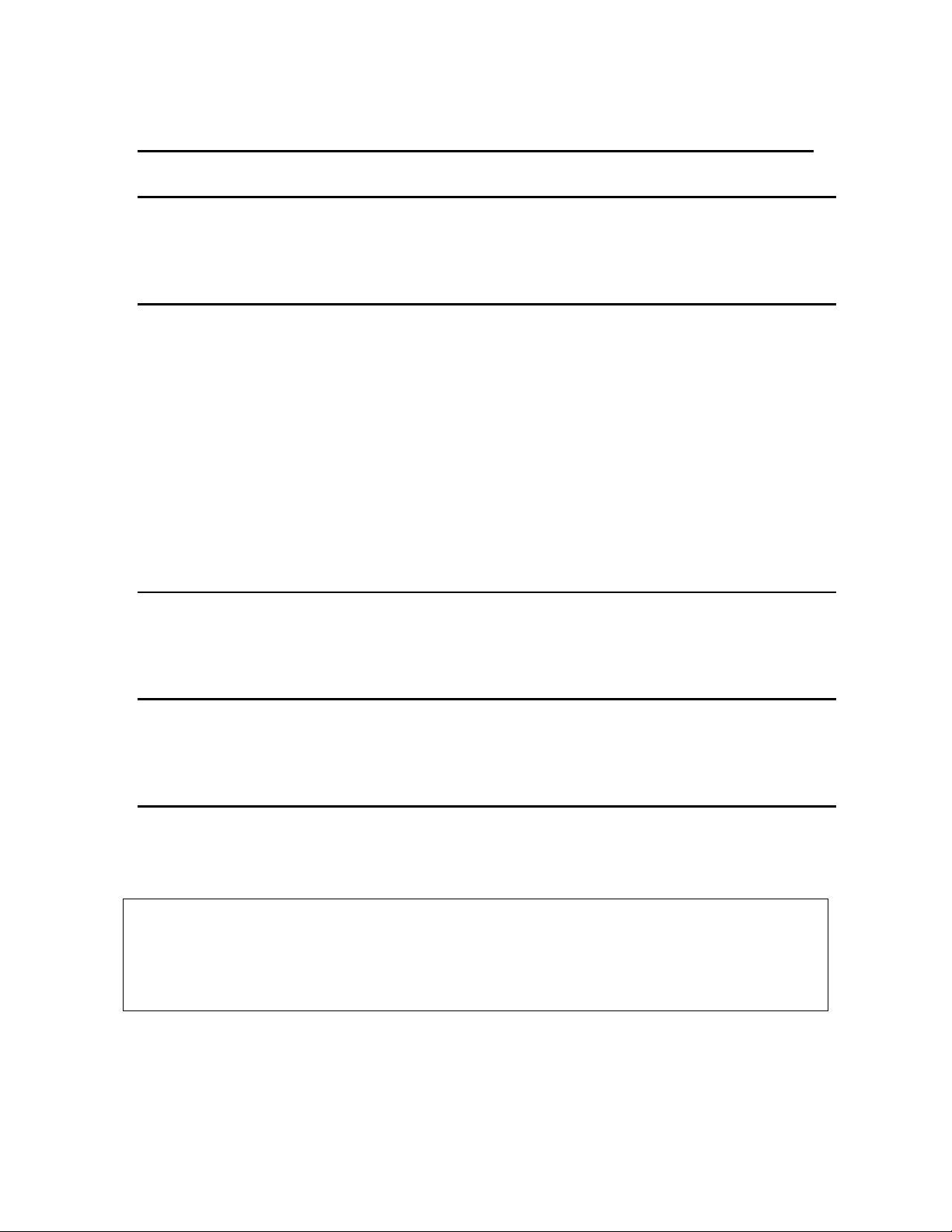
2.2 CONNECTING YOUR SONDE

There are a number of ways in which you may connect the sondes to various computers, data collection devices and VT-100 terminal emulators. To utilize the configuration that will work best for your application, make sure that you have all of the components that are necessary. The following list and diagrams (Figures 1-4) are a few possible configurations.

 Sonde to Lab Computer (recommended for initial setup)  Sonde to Data Collection Platform  Sonde to Portable Computer  Sonde to YSI 650 MDS Display/Logger

Figure 1

YSI Incorporated Environmental Monitoring Systems Operations Manual 2-2

Sondes Section 2

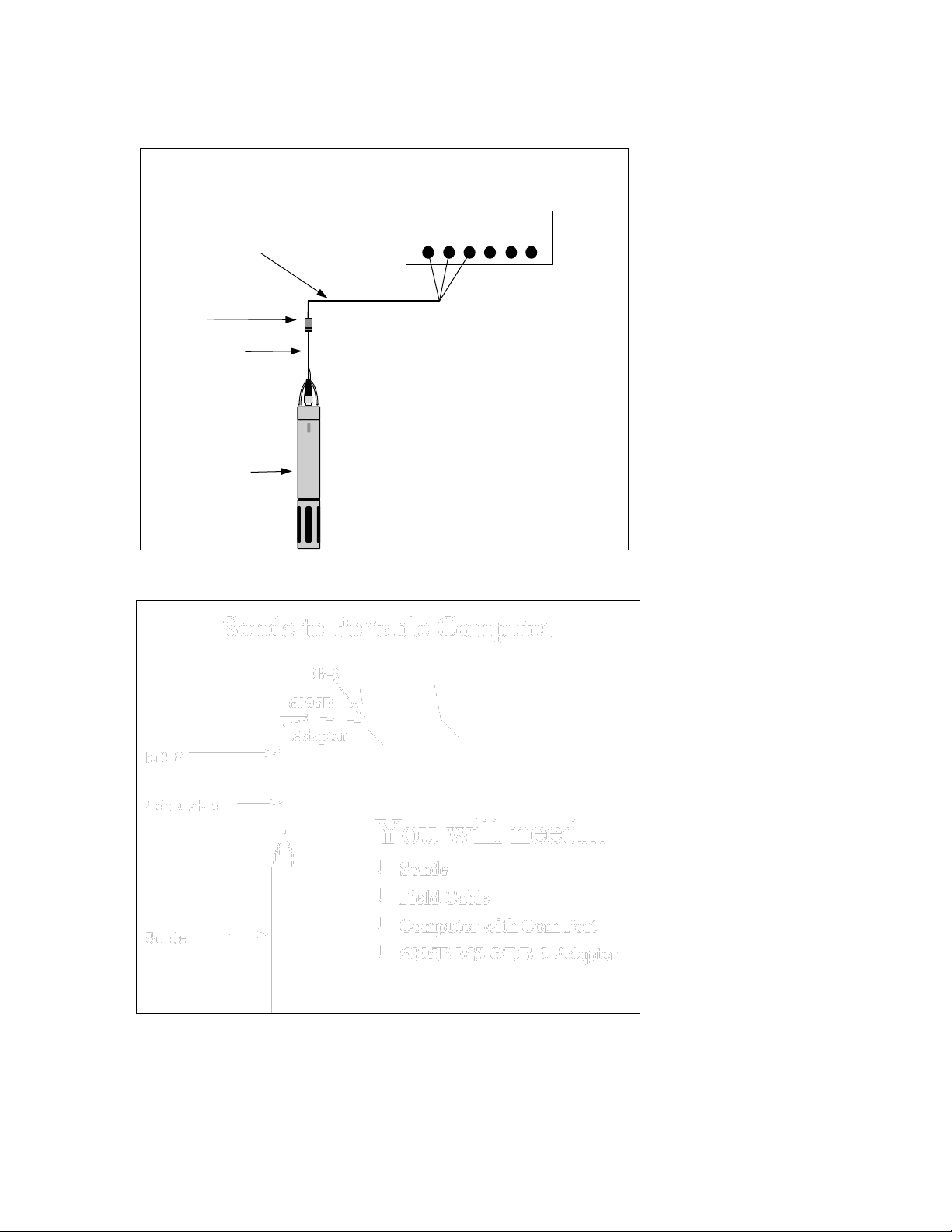
Sonde to Data Collection Platform

You will need...



Sonde



Field Cable



6096 Adapter with leads



Data Collection Platform

6096 MS-8 Adapter with Flying Leads

DCP

Field Cable

MS-8

Sonde

YSI 692 0

Figure 2

Figure 3

YSI Incorporated Environmental Monitoring Systems Operations Manual 2-3

Sondes Section 2

Sonde to 650 Display/Logger

You will need...



Sonde



Field Cable



650 MDS Display/Logger

YSI 650 operates on C-cells or rechargeable batteries.

650 MDS

610-DM

Environmental

Monitoring

Systems

Field Cable

Sonde

YS I 69

+ + -

MS-8

Figure 4

YSI Incorporated Environmental Monitoring Systems Operations Manual 2-4

ADD DI OR DISTILLED

WATER

PROTECTIVE CAP

DRY MEMBRANE

Sondes Section 2

2.3 PREPARING THE SONDE FOR USE

To prepare the sonde for calibration and operation, you need to install probes (sensors) into the connectors on the sonde bulkhead. In addition to probe installation, you need to install a new membrane on the YSI 6562 DO Probe if you are using this item. It is recommended that you install the DO membrane before installing the probe onto the bulkhead. For membrane changes in the future, you may be able to perform this operation without removing the DO probe. This will largely depend on whether the other installed probes interfere with your ability to install a membrane. The next step is providing power for the sondes, through batteries or line power, and then connecting a field cable. The four steps necessary for getting your sonde ready for use are listed below.

Step 1 Installing the Dissolved Oxygen Membrane – Section 2.3.1 Step 2 Installing the Probes – Section 2.3.2 Step 3 Supplying Power – Section 2.3.3 Step 4 Connecting a Field Cable – Section 2.3.4

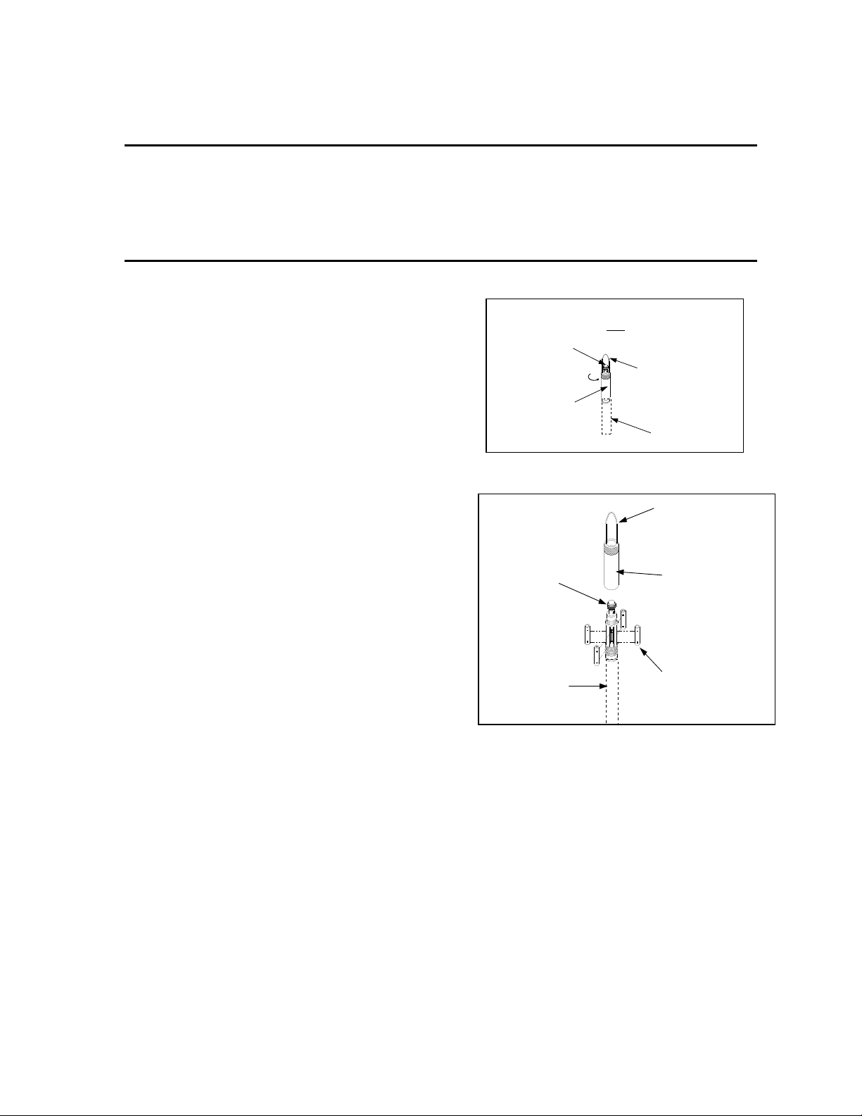
2.3.1 STEP 1 - INSTALLING THE DISSOLVED OXYGEN MEMBRANE

Note: If you are using a ROX Optical DO sensor for your applications, please skip to Section 2.3.2 at this time.

The 6562 Rapid Pulse Polarographic DO probe is shipped with a protective dry membrane on the sensor tip held in place by an O-ring. Remove the O-ring and membrane. Handle the probe with care. It is very important not to scratch or contaminate the sensor tip. See Section 2.10.2, Probe Care and Maintenance, for information on how often the membrane should be replaced.

Unpack the YSI 6562 DO Probe Kit and follow the instructions below.

Open the membrane kit and prepare the electrolyte solution. Dissolve the KCl in the dropper bottle by filling it to the neck with deionized or distilled water and shaking until the solids are fully dissolved. After the KCl is dissolved, wait a few minutes until the solution is free of bubbles.

Figure 5 Figure 6

The DO membrane can be installed with the DO probe either free or installed in the sonde. Both methods are described in detail below. CAUTION: If you install the membrane with the probe not installed in

the sonde, be sure that the protective cap is installed on the probe end away from the sensor face to ensure that the connector is not contaminated with electrolyte.

YSI Incorporated Environmental Monitoring Systems Operations Manual 2-5

Sondes Section 2

345

DO MEMBRANE INSTALLATION WITH THE PROBE NOT INSTALLED IN THE SONDE

Remove the protective cap and the dry membrane from the YSI 6562 Dissolved Oxygen probe.

Make sure that the protective cap is installed on the connector end of the probe. Do not allow the electrolyte solution to wet the probe‟s connector and O-ring seal areas. This solution is extremely corrosive to the connector and is difficult to remove.

Before using any electrolyte, wrap a clean, dry paper towel around the capped probe to catch any spilled electrolyte. Hold the probe in a vertical position and apply a few drops of KCl solution to the tip. The fluid should completely fill the small moat around the electrodes and form a meniscus on the tip of the sensor. Be sure no air bubbles are stuck to the face of the sensor. If necessary, shake off the electrolyte and start over. Figure 7 Secure a membrane between your left thumb and the probe body. Always handle the membrane with care, touching it only at the ends.

With the thumb and forefinger of your right hand, grasp the free end of the membrane. With one continuous motion, gently stretch it up, over, and down the other side of the sensor. The membrane should conform to the face of the sensor.

Secure the end of the membrane under the forefinger of your left hand.

Roll the O-ring over the end of the probe, being careful not to touch the membrane surface with your fingers. There should be no wrinkles or trapped air bubbles. Small wrinkles may be removed by lightly tugging on the edges of the membrane. If bubbles are present, remove the membrane and repeat steps 3-8.

Trim off any excess membrane with a sharp knife or scissors. Rinse off any excess KCl solution, but be careful not to get any water in the connector.

If you are concerned that electrolyte may have dripped onto the Oring seal area, probe connector, or bulkhead connectors, rub the area clean with paper towels wetted with Deionized water and then dry the affected area with a final dry towel, compressed air blasts, or rinse with fresh alcohol.

NOTE: You may find it more convenient to mount the probe vertically in a vise with rubber jaws while applying the electrolyte and membrane to the sensor tip.

YSI Incorporated Environmental Monitoring Systems Operations Manual 2-6

Sondes Section 2

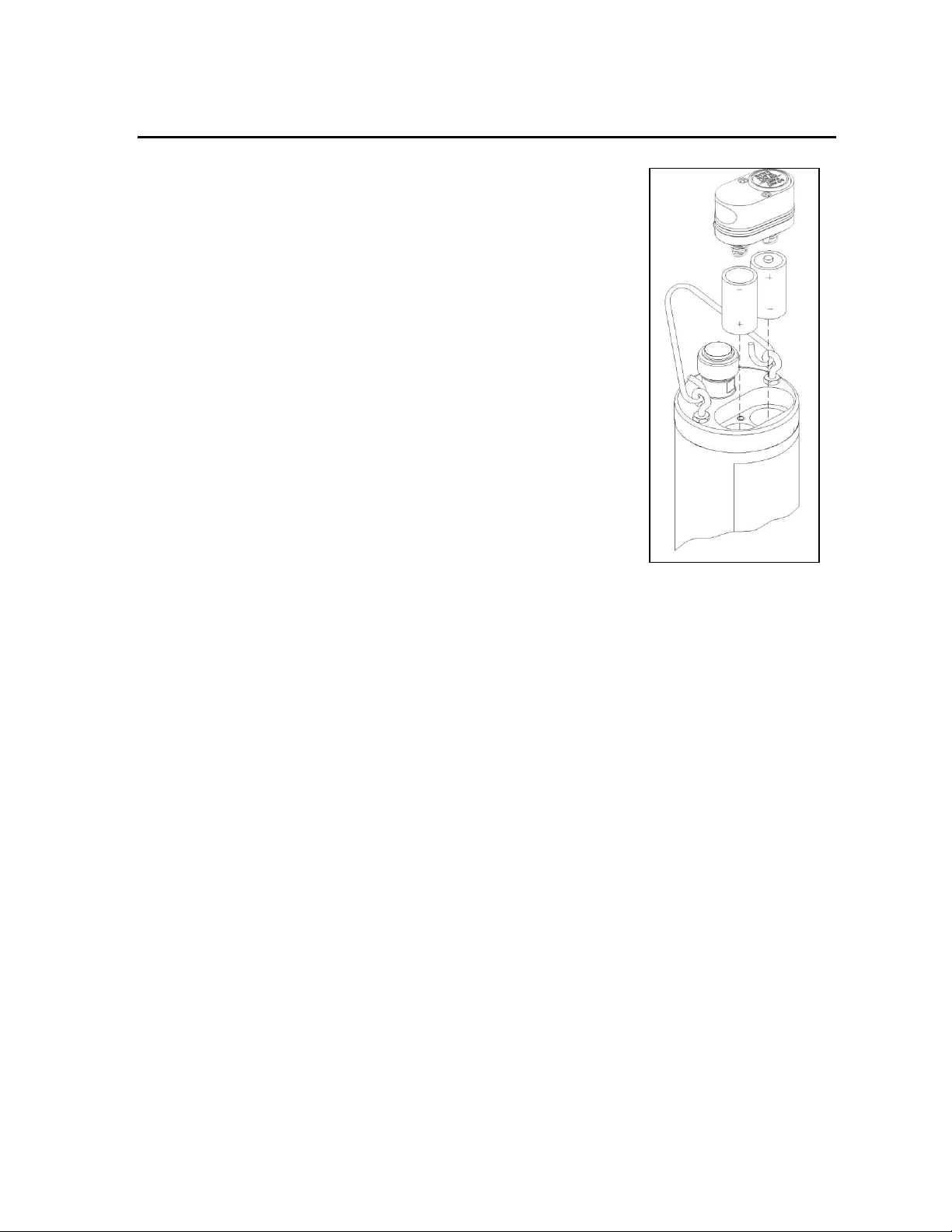
DO MEMBRANE INSTALLATION WITH THE PROBE INSTALLED IN THE SONDE

Secure the sonde in a vertical position using a vise or a clamp and ring stand such that the sensors are upright. Remove the probe guard from the sonde.

Remove the old DO membrane and clean the probe tip with water and lens cleaning tissue. Make sure to remove any debris or deposits from the O-ring groove.

Using the dropper bottle of electrolyte supplied, place electrolyte on the DO probe tip until a high meniscus is formed as shown in Figure 8 below.

Figure 8 Figure 9

Hold the membrane so that all four corners are supported, but do not stretch the membrane laterally.

Position the membrane over the probe, keeping it parallel to the probe face as shown in Figure 9 above.

Using one continuous downward motion, stretch the membrane over the probe face as shown. See Figure 10 below. Do not hesitate to stretch the membrane.

Figure 10 Figure 11

Install a new O-ring by placing one side of the O-ring in the groove and rolling into place across the membrane and into the groove on the opposite side of the probe face. Avoid touching the probe face with

YSI Incorporated Environmental Monitoring Systems Operations Manual 2-7

Sondes Section 2

TRANSPORT CUP

BULKHEAD WITH

PROBE PORT PLUGS

your fingers. Once the O-ring is in position, squeeze it every 90 degrees to equalize the tension. See Figure 11 above. DO NOT USE GREASE OR LUBICANT OF ANY KIND ON THE O-RING.

Using a hobby knife or a scalpel, trim the excess Teflon from the membrane, making your cut about 1/8 inch below the O-ring as shown in Figure 12 below. A razor blade can be used for the cut if no knife or scalpel is available.

Figure 12 Figure 13

If the installation has been done properly, the finished product should have no bubbles, wrinkles, or tears as shown in Figure 13 above.

NOTE: Observe the following cautions to assure that your membrane installation is proper:

 Secure the sonde tightly so that it will not move during membrane installation.

 Wash hands before installation and do not allow finger oils or O-ring lubricant to touch the probe face

or the membrane.

 Use caution when replacing the probe guard that you do not touch the membrane. If you suspect that

the membrane has been damaged, replace it immediately.

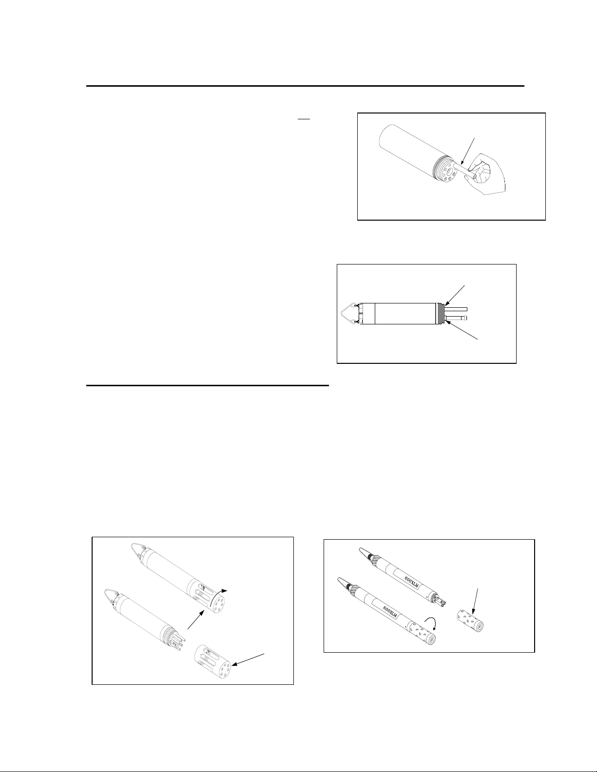
2.3.2 STEP 2 - INSTALLING THE PROBES

Remove the calibration cup from your sonde by hand as shown in Figure 14, to expose the bulkhead.

Figure 14

YSI Incorporated Environmental Monitoring Systems Operations Manual 2-8

Sondes Section 2

OPTIC

PORT PLUG

INSTALLATION TOOL

DO, COND., & pH/ORP PORT PLUGS

INSTALLATION

TOOL

ISE PORT PLUG

PLIERS

(SLIP JAWS)

REMOVING THE PORT PLUGS

Using the long extended end of the probe installation tool supplied in the YSI 6570 Maintenance Kit, remove the port plugs. Save all the port plugs Figure 15 for possible future use.

There are a variety of probe options for the sondes. Figures 15, 16 and 17 illustrate the uses of the common tool for port plug removal. Note that this tool will also be used to install the various probes.

If the tool is misplaced or lost, you may use 7/64” and 9/64” hex keys as substitutes.

Figure 16 Figure 17

Figure 18 NOTE: You may need pliers to remove the ISE port plugs, but do not use pliers to tighten the ISE probes. Hand-tighten only.

Now refer to Figures 19-24 to find the probe locations in your sonde.

YSI Incorporated Environmental Monitoring Systems Operations Manual 2-9

Sondes Section 2

DISSOLVED OXYGEN 6562

CONDUCTIVITY/ TEMPERATURE 6560

ALL ISE PROBES

Cond./Temp.

Optic T

pH/ORP

ISE‟s

Dissolved Oxygen

Optic C

600XL & 600XLM SONDE BULKHEAD

3 Port Sonde: 1 Rapid Pulse DO, 1 Conductivity/Temperature, and 1 pH/ORP

Figure 19

 6562 Dissolved oxygen probe = 3-pin connector  6560 Conductivity/Temperature = 6-pin connector  6561 pH probe = 4 pin connector  6565 Combo pH/ORP probe = 4 pin connector

6600V2-2 SONDE BULKHEAD

8 Port Sonde: 1 Rapid Pulse DO, 1 Conductivity/Temperature, 2 Optical, 3 ISE, 1 pH/ORP

Figure 20A

 6562 Dissolved oxygen probe = 3-pin connector  6560 Conductivity/Temperature = 6-pin connector  6561 or 6561FG pH probe = 4 pin connector  6565 or 6565FG pH/ORP probe = 4 pin connector  6566 Fouling Resistant pH/ORP probe = 4 pin connector  6882 Chloride Probe = leaf spring connector  6883 Ammonium Probe = leaf spring connector  6884 Nitrate Probe = leaf spring connector  6026 Turbidity Probe, Wiping = 8 pin connector  6136 Turbidity Probe, Wiping = 8 pin connector  6025 Chlorophyll Probe, Wiping = 8 pin connector  6130 Rhodamine WT Probe, Wiping = 8 pin connector  6150 Optical Dissolved oxygen probe = 8 pin connector  6131 PC-Blue-green Algae probe = 8 pin connector  6132 PE-Blue-green Algae probe = 8 pin connector

YSI Incorporated Environmental Monitoring Systems Operations Manual 2-10

Sondes Section 2

Cond/Temp – 6 pin

pH/ORP – 4 pin

Cond//Temp – 6 pin

pH/ORP – 4 pin Rapid Pulse DO – 3 pin

6600EDS V2-2 SONDE BULKHEAD

5 Port Sonde: 1 Rapid Pulse DO, 1 Conductivity/Temperature, 2 Optical, 1 pH/ORP

Figure 20B

 6562 Dissolved oxygen probe = 3-pin connector  6560 Conductivity/Temperature = 6-pin connector  6561 or 6561FG pH probe = 4 pin connector  6565 or 6565FG pH/ORP probe = 4 pin connector  6566 Fouling Resistant pH/ORP probe = 4 pin connector  6026 Turbidity Probe, Wiping = 8 pin connector  6136 Turbidity Probe, Wiping = 8 pin connector  6025 Chlorophyll Probe, Wiping = 8 pin connector  6130 Rhodamine WT Probe, Wiping = 8 pin connector  6150 Optical Dissolved oxygen probe = 8 pin connector  6131 PC-Blue-green Algae probe = 8 pin connector  6132 PE-Blue-green Algae probe = 8 pin connector

6600V2-4 SONDE BULKHEAD

6 Port Sonde: 1 Conductivity/Temperature, 4 Optical, 1 pH/ORP

Figure 20C

 6560 Conductivity/Temperature = 6-pin connector  6561 or 6561FG pH probe = 4 pin connector  6565 or 6565FG pH/ORP probe = 4 pin connector  6566 Fouling Resistant pH/ORP probe = 4 pin connector  6026 Turbidity Probe, Wiping = 8 pin connector  6136 Turbidity Probe, Wiping = 8 pin connector  6025 Chlorophyll Probe, Wiping = 8 pin connector  6130 Rhodamine WT Probe, Wiping = 8 pin connector  6150 Optical Dissolved oxygen probe = 8 pin connector  6131 PC-Blue-green Algae probe = 8 pin connector  6132 PE-Blue-green Algae probe = 8 pin connector

YSI Incorporated Environmental Monitoring Systems Operations Manual 2-11

Sondes Section 2

MOUNTING SCREW

DISSOLVED

OXYGEN

COND/TEMP

ISE1/ISE2

pH/ORP

ISE3 ISE4

ISE5

OPTICAL

6820V2-1 & 6920V2-1 SONDE BULKHEADS

7 Port Sonde: 1 Rapid Pulse DO, 1 Conductivity/Temperature, 1 Optical, 1 pH/ORP, 3 ISE

Figure 21A

6820V2-2 & 6920V2-2 SONDE BULKHEADS

5 Port Sonde: 1 Conductivity/Temperature, 2 Optical, 1 pH/ORP, 1 ISE

Figure 21B

 6560 Conductivity/Temperature = 6-pin connector  6561 or 6561FG pH probe = 4 pin connector  6565 or 6565FG pH/ORP probe = 4 pin connector  6566 Fouling Resistant pH/ORP probe = 4 pin connector  6882 Chloride Probe = leaf spring connector  6883 Ammonium Probe = leaf spring connector  6884 Nitrate Probe = leaf spring connector  6026 Turbidity Probe, Wiping = 8 pin connector  6136 Turbidity Probe, Wiping = 8 pin connector  6025 Chlorophyll Probe, Wiping = 8 pin connector  6130 Rhodamine WT Probe, Wiping = 8 pin connector  6150 Optical Dissolved oxygen probe = 8 pin connector  6131 PC-Blue-green Algae probe = 8 pin connector  6132 PE-Blue-green Algae probe = 8 pin connector

YSI Incorporated Environmental Monitoring Systems Operations Manual 2-12

Sondes Section 2

TEMPERATURE

pH GLASS

pH REFERENCE 6850

CONDUCTIVITY

DISSOLVED OXYGEN

TEMPERATURE

pH GLASS/ORP

pH REFERENCE 6850

CONDUCTIVITY

DISSOLVED OXYGEN

Conductivity Temperature

Depth

600LS BULKHEAD

If are working with a 600LS, all sensors will have been installed at the factory.

600R BULKHEAD

If are working with a 600R sonde, your instrument will arrive with the probes installed.

600QS BULKHEAD

If are working with a 600QS sonde, your instrument will arrive with the probes installed.

YSI Incorporated Environmental Monitoring Systems Operations Manual 2-13

Figure 21C

Figure 22

Figure 23

Sondes Section 2

LUBRICATE O-RINGS

Conductivity Port Optical Port

Temperature Sensor

600 OMS V2-1 BULKHEAD

Figure 24

The conductivity sensor (module/port) for the 600 OMS V2-1 is factory installed. Optical probes (turbidity, chlorophyll, rhodamine WT, ROX optical DO, BGA-PC, and BGA-PE) are threaded into the optical port on the bottom of the sonde by the user.

LUBRICATE O-RINGS

Apply a thin coat of O-ring lubricant, supplied in the YSI 6570 Maintenance Kit, to the O-rings on the connector side of each probe that is to be installed.

Figure 25

CAUTION: Make sure that there are NO contaminants

between the O-ring and the probe. Contaminants that are present under the O-ring may cause the O-ring to leak when the sonde is deployed.

NOTE: Before installing any probe into the sonde bulkhead, be sure that the probe port is free of

moisture. If there is moisture present, you may use a can of compressed air to blow out the remaining moisture.

YSI Incorporated Environmental Monitoring Systems Operations Manual 2-14

Sondes Section 2

OPTIC

PROBE

INSTALLATION

TOOL

PROBE INSTALLATION

TOOL

DO PROBE

INSTALLING THE TURBIDITY, CHLOROPHYLL, RHODAMINE WT , BGA-PHYCOCYANIN, BGAPHYCOERYTHRIN, AND ROX OPTICAL DISSOLVED OXYGEN PROBES

If you are using any of optical probes listed, it is recommended that the optical sensors be installed first. If you are not installing one of these probes, do not remove the port plug, and go on to the next probe installation. Figure 26 All optical probes, 6136 turbidity, 6025 chlorophyll, 6130 Rhodamine WT, 6131 Phycocyanin Blue-green algae, 6132 Phycoerythrin-Blue-green algae, and 6150 ROX Optical DO are installed in the same way. Install the probe into the center port, seating the pins of the two connectors before you begin to tighten. Tighten the probe nut to the bulkhead using the short extended end of the tool supplied with the probe. Do not over-tighten.

CAUTION: Be careful not to cross-thread the probe nut.

The YSI 6820V2-1 and 6920V2-1 sondes can accept a single turbidity, chlorophyll, Rhodamine WT, BGAPC, BGA-PE, or ROX DO probe. The 6600V2-2, 6600EDS V2-2, 6820V2-2, and 6920V2-2 sondes can accept and utilize two of the six optical sensors at the same time. The two optical ports of these sondes are labeled “T” and “C” on the sonde bulkhead. Each port can accept any of the six sensors so be sure to remember which sensor was installed in which port so that you will later be able to set up the sonde software correctly. The 6600V2-4 sonde can accept and utilize four of the six optical sensors at the same time. The four optical ports of this sonde are labeled “T” , “C”, “B”, and “O” on the sonde bulkhead. Each port can accept any of the six sensors so be sure to remember which sensor was installed in which port so that you will later be able to set up the sonde software correctly.

INSTALLING THE 6562 RAPID PULSE DISSOLVED OXYGEN PROBE, CONDUCTIVITY/TEMP AND pH/ORP PROBES

Figure 27 Insert the probe into the correct port and gently rotate the probe until the two connectors align.

The probes have slip nuts that require a small probe installation tool to tighten the probe. With the connectors aligned, screw down the probe nut using the long extended end of the probe installation tool. Do not over-tighten.

CAUTION: Do not cross thread the probe nut.

YSI Incorporated Environmental Monitoring Systems Operations Manual 2-15

Sondes Section 2

PROBE NUT TO SEAT

ON BULKHEAD

PROBE BODY TO SEAT

ON BULKHEAD

DO PROBE

ISE PROBE

BULKHEAD

(PROBES INSTALLED)

PROBE GUARD

TURN CLOCKWISE BY

HAND TO SECURE

PROBE GUARD

ISE PROBE

INSERT ISE PROBE,

SCREW IN AND TIGHTEN WITH FINGERS.

INSTALLING THE ISE PROBES

Figure 28 The Ammonium, Nitrate and Chloride ISE probes do not have slip nuts and should be installed without tools. Use only your fingers to tighten. Any ISE probe can be installed in any of the three ports labeled “3”, “4”, and “5” on the sonde bulkhead of the 6820V2-1, 6920V2-1, and 6600V2-2 sondes or the single ISE port on the 6820V2-2 and 6920V2-2 bulkheads. Be sure to remember which sensor was installed in which port so that you will later be able to set up the sonde software correctly.

Figure 29 IMPORTANT: Make sure that the probe nut or probe body of the ISE probes are seated directly on the sonde bulkhead. This will ensure that connector seals will not allow leakage.

INSTALLING THE PROBE GUARD

Included with each sonde is a probe guard. The probe guard protects the probes during calibration and measurement procedures. Once the probes are installed, install this guard by aligning it with the threads on the bulkhead and turn the guard clockwise until secure.

CAUTION: Be careful not to damage the Rapid Pulse DO membrane during installation of the probe

guard.

Figure 30 shows the YSI 6820V2-1/6820V2-2/6920V2-1/6920V2-2 probe guard; the guard for the 6600V2-2/6600V2-4 is similar. The YSI 600R, 600QS, 600XL and 600XLM probe guards resemble Figure 31.

Figure 30 Figure 31

YSI Incorporated Environmental Monitoring Systems Operations Manual 2-16

Sondes Section 2

2.3.3 STEP 3 - POWER

Some type of external power supply is required to power the YSI 600R, 600QS, 600XL 6820V2-1, and the non-battery version of the 600 OMS V2-1sondes. The YSI 6920V2-1, 6920V2-2, 6600V2-2, 6600EDS V2-2, 6600V2-4, 600XLM, and battery version of the 600 OMS V2-1sondes have internal batteries or can run on external power.

If you have purchased a YSI 650 MDS display/logger, attaching your sonde to the display/logger will allow your sonde to be powered from the batteries or the external power of the display/logger. See Section 3, Displays/Loggers, for power options.

The battery-powered version of this instrument is powered by alkaline batteries, which the user must remove and dispose of when the batteries no longer power the instrument. Disposal requirements vary by country and region, and users are expected to understand and follow the battery disposal requirements for their specific locale.

The circuit board in this instrument contains a manganese dioxide lithium "coin cell" battery that must be in place for continuity of power to memory devices on the board. This battery is not user serviceable or replaceable. When appropriate, an authorized YSI service center will remove this battery and properly dispose of it, per service and repair policies.

POWER FOR LAB CALIBRATION

A YSI 6038 (110 VAC) or 6651 (64-240 VAC) Power Supply is required for sondes without internal batteries when using them with a PC for calibration and setup. Sondes with internal batteries do not require a power supply, but using the sonde with a power supply in the lab is often convenient and extends battery life. Most adapters include a short pigtail for power that plugs into the power supply. After attaching the four-pin connector from the power supply to the pigtail, simply plug the power supply into the appropr iate AC outlet.

See Section 2.2, Connecting Your Sonde, for specific information on cables, adapters and power supplies required for connecting your sonde to various devices.

Figure 32

The system configuration best suited for initial setup is shown in Figure 32.

YSI Incorporated Environmental Monitoring Systems Operations Manual 2-17

Sondes Section 2

BAIL

BULKHEAD CONNECTOR WITH CAP

AA BATTERIES x 4 (NOTE POLARITY)

SONDE BODY (NOT SHOWN)

SCREW ON BATTERY CAP

BATTERY

CAP

BULKHEAD

CONNECTOR

SONDE

BODY

DO NOT USE BAIL FOR LEVERAGE

WHEN REMOVING BATTERY CAP!

BAIL

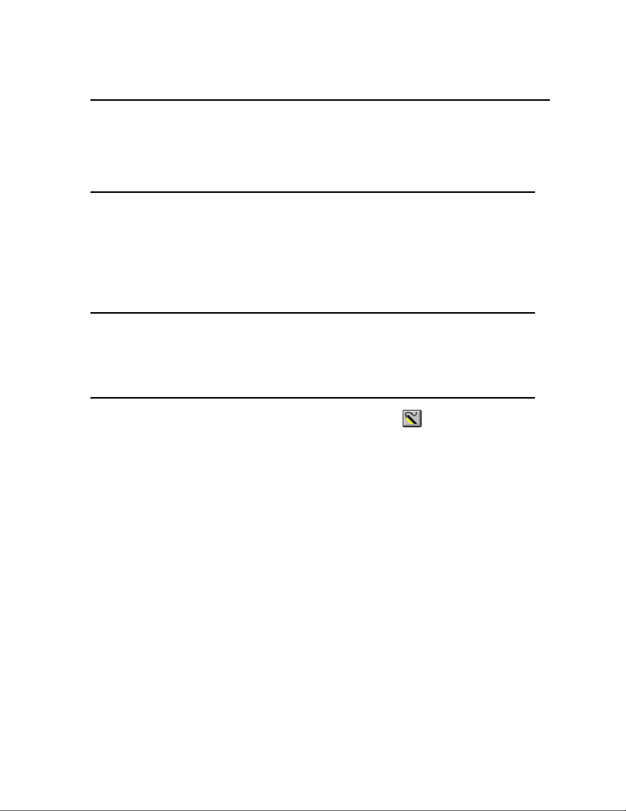
INSTALLING BATTERIES

The 600XLM, 6600V2-2, 6600EDS V2-2, 6600V2-4, 6920V2-1, 6920V2-2 and battery version of the 600 OMS V2-1are the sondes that use alkaline batteries for power. A set of batteries is supplied with each of these sondes. If you do not have one of these sonde model types, you may skip this section.

INSTALLING BATTERIES INTO THE YSI 600XLM OR 600 OMS V2-1 SONDES

Figure 33 To install 4 AA-size alkaline batteries into the sonde, refer to the following directions and Figure 33.

Grasp the cylindrical battery cover and unscrew by hand. Then slide the battery lid up and over the bulkhead connector. Insert batteries, paying special attention to polarity. Labeling on the battery compartment posts describes the orientation. It is usually easiest to insert the negative end of battery first and then “pop” the positive terminal into place.

Figure 34 Check the O-ring and sealing surfaces for any contaminants that could interfere with the O-ring seal of the battery chamber.

CAUTION: Make sure that there are NO contaminants

between the O-ring and the sonde. Contaminants that are present under the O-ring may cause the O-ring to leak when the sonde is deployed.

Lightly lubricate the o-ring on the outside of the battery cover. DO NOT lubricate the internal o-ring.

Return the battery lid and tighten by hand.

DO NOT OVER-TIGHTEN.

YSI Incorporated Environmental Monitoring Systems Operations Manual 2-18

Sondes Section 2

Align seal to groove

Retaining Tabs

Middle tabs

INSTALLING BATTERIES INTO THE YSI 6600V2-2, 6600EDS V2-2, AND 6600V2-4 SONDES

Figure 35

IMPORTANT SAFETY FEATURE: The 116003 battery lid for the 6600V2-2, 6600EDS V2-2, and 6600V2-4 is equipped with a safety pressure-release valve. The valve will vent off any pressure build up in the battery compartment from waste gas that could be created by battery failure, improperly marked or installed batteries, flooding, and dead or heavily discharged batteries. Pressure from the waste gas can deform the battery compartment and cause the sonde to shatter, projecting fragments from the sonde casing in all directions. People near a sonde that shatters could suffer serious puncture wounds and serious eye injuries. DO NOT defeat this safety feature by blocking the valve or painting over or in close proximity to the valve. DO NOT attempt to disassemble the safety valve.

Install 8 C-size alkaline batteries according to the following directions and Figure 35.

Using the 9/64” hex driver supplied with the 6600V2-2, 6600EDS V2-2 and 6600V2-4 loosen the battery lid screws.

NOTE: The battery lid screws are captive. It is not necessary to remove them from the lid completely.

Remove the battery lid and install the batteries, as shown. If installing or replacing the batteries, test batteries for proper polarity and voltage and observe the correct polarity before installing the batteries into the battery chamber.

CAUTION: Be sure the orange O-ring is installed in the groove of the lid. The o-ring is designed with retention tabs to prevent it from falling out of the grove during installation. Check the O-ring and sealing surfaces for any contaminates which could interfere with the O-ring seal of the battery chamber. Remove any contaminates present. Also clean the protective O-rings which are located the side of the battery lid. Apply a small amount of grease to the threads of each screw to prevent binding. See the next section and Figures 35A through 35L for details on proper installation of the battery lid o-ring.

The updated face seal for the 6600 sonde battery lid incorporates six retaining tabs to hold the face seal in the seal groove during installation, allowing consistent and effective sealing after battery replacement. In order for this feature to work properly, the retaining tabs must be correctly seated in the battery lid‟s seal groove to prevent it from becoming dislodged during handling. If the seal is not installed correctly it can fall out of its groove during battery lid installation and then can be crushed during assembly. This may cause damage to the seal and cause battery compartment flooding when the sonde is deployed. The following procedure is a recommended method to properly retain the seal in its groove:

1. Place seal on the battery lid groove so that it

follows the profile of the groove and is centered about the two middle retaining tabs.

Figures 35A and 35B

YSI Incorporated Environmental Monitoring Systems Operations Manual 2-19

Sondes Section 2

Press tabs into groove

Stretch seal and press tab

into groove

Stretch seal and press tab

into groove

Press on tabs to verify they

have been seated

2. Press two of the outermost retaining tabs down

into the groove. It should be clear that the retaining tabs have recessed into the groove along with the seal so that the tabs outermost edges are at or below the battery lid‟s mounting surface.

Figures 35C and 35D

3. Press the remaining two outermost retaining tabs

into the groove and check to make sure the tabs have been recessed as before. Verify that the other two previously seated retaining tabs have not been forced from their position in the groove.

Figures 35E and 35F

4. Place your thumbs on the seal about a ¼” or so

from the sides of the center retaining tab and press the seal down into the groove while sliding your thumbs towards each other. This stretches the seal to fit the profile of the groove allowing the center tab to be seated properly. You may need to use the tip of one of your thumbs to finish pressing the tab into place.

Figures 35G and 35H

5. Press the remaining middle retaining tab into the

groove as before and verify that none of the other retaining tabs have been forced from their positions in the groove during this part of the seal installation.

Figures 35I and 35J

6. To ensure that all the retaining tabs are properly

seated in the seal groove you can apply pressure to the seal forcing it into the groove at the location of each tab. This will further seat each tab into the groove allowing it to capture the seal.

Figures 35K and 35L

CAUTION: Before installing the battery lid, ensure that the pressure release valve is closed.

If the pressure release valve is open, DO NOT install (see Figures 35M and 35N). The valve

YSI Incorporated Environmental Monitoring Systems Operations Manual 2-20

Sondes Section 2

BAIL

SONDE BODY

BATTERY CAP

GRASP BAIL WITH HAND.

TURN COUNTERCLOCKWISE TO LOOSEN.

BULKHEAD CONNECTOR WITH CAP

Figure 35M: Closed valve

OK to Deploy

Figure 35N: Open valve

DO NOT Deploy

cannot be reset and the battery lid must be replaced before sonde deployment. Contact YSI Technical Support for instructions.

Lightly lubricate the o-rings on the outside of the battery cover. DO NOT lubricate the orange internal oring.

Return the battery lid and HAND tighten the screws with the hex driver until snug. DO NOT OVER

TIGHTEN.

CAUTION: Over-tightening the screws may cause the battery compartment to flood. Do NOT use power tools to tighten the battery lid screws.

With the battery cover installed and secured, check the battery voltage in the sondes Status Menu. The voltage must be 12.0 volts or higher with new cells. A voltage less then 12.0 volts could indicate that a cell was installed upside down or that one of the cells is not at full strength.

CAUTION: Remove Batteries When Not in Use. As with any battery-powered instrumentation, batteries should be removed before short or long-term storage. Even with the new battery lid, batteries can leak, releasing toxic and corrosive battery acid and damaging equipment.

INSTALLING BATTERIES IN THE 6920V2-1 AND 6920V2-2 SONDES

To install the 8 AA-size alkaline batteries into the sonde, refer to the following directions and Figures 36 and 37. Figure 36

Position the bail so that it is perpendicular to the sonde and use it as a lever to unscrew the battery cap by hand. Then slide the battery lid up and over the bulkhead connector.

Insert batteries, paying special attention to polarity. Labeling on the top of the sonde body describes the orientation.

YSI Incorporated Environmental Monitoring Systems Operations Manual 2-21

+--

BATTERY CAP

BULKHEAD

CONNECTOR

BAIL

O-RINGS

REMOVE

WATERPROOF CAP

SONDE

CONNECTOR

FIELD CABLE

CONNECTOR

BAIL

STRAIN RELIEF

CONNECTOR

Sondes Section 2

Check the O-rings and sealing surfaces for any contaminants that could interfere with the seal of the battery chamber.

CAUTION: Make sure that there are NO contaminants between

the O-ring and the sonde. Contaminants that are present under the O-ring may cause the O-ring to leak when the sonde is deployed.

Lightly lubricate the o-rings on the bottom of the threads and on the connector stem as shown in Figure 37.

Return the battery lid and tighten by hand. DO NOT OVER-

TIGHTEN.

Figure 37

2.3.4 STEP 4 - CONNECTING A FIELD CABLE

Figure 38 All YSI 6600V2-2, 6600EDS V2-2, 6600V2-4, 6920V2-1, 6920V2-2, 6820V2-2, 600XLM, 600QS, and 600 OMS V2-1sondes have a sonde-mounted cable connector for attachment of the field cable. Some versions of the 600R, 600XL, and 6820V2-1 sondes also have this connector.

However, some versions of the YSI 600R, 600XL, and 6820V2-1sondes have permanently attached “integral” cables. If your sonde has a cable that is non-detachable, the next section will not be relevant.

To attach a field cable to the sonde connector, remove the waterproof cap from the sonde connector and set it aside for later reassembly during deployment or storage. Then connect your field cable to the sonde connector.

A built-in “key” will ensure proper pin alignment. Rotate the cable gently until the “key” engages and then tighten the connectors together by rotating clockwise. Attach the strain relief connector to the sonde bail. Rotate the strain relief connector nut to close the connector's opening.

For all of the sondes, the other end of the cable is a military-style 8-pin connector (MS-8). Through use of a YSI 6095B MS-8 to DB-9 adapter, the sonde may be connected to a computer for setup, calibration, realtime measurement, and uploading files.

This MS-8 connector also plugs directly into the 650 MDS display/logger. This instrument contains a microcomputer that allows it to be used in a similar manner to that of a terminal interface to a PC.

As an alternative to the field cable, you may use a YSI 6067B calibration cable for laboratory interaction with the sonde. In this case, simply plug the proper end of the cable into the sonde connector and attach the DB-9 connector of the cable to the Com port of your computer.

YSI Incorporated Environmental Monitoring Systems Operations Manual 2-22

Sondes Section 2

CAUTION: The 6067B cable is for laboratory use only -- it is not waterproof and should not be submersed!

Sondes that are equipped with level sensors use vented cables. See Appendix G, Using Vented Level, for detailed information.

YSI Incorporated Environmental Monitoring Systems Operations Manual 2-23

Sondes Section 2

2.4 ECOWATCH FOR WINDOWS -GETTING STARTED

This section will describe how to get started with EcoWatch for Windows, but detailed information is provided in Section 4, EcoWatch for Windows, or a convenient Windows Help section that is part of the software. It is recommended that you thoroughly read Section 4 or use the Help function for a comprehensive understanding of EcoWatch for Windows.

2.4.1 INSTALLING ECOWATCH FOR WINDOWS

EcoWatch for Windows software must be used with an IBM-compatible PC with a 386 (or better) processor. The computer should also have at least 4MB of RAM and Windows Version 3.1 or later.

Place the EcoWatch for Windows compact disk in your CD ROM drive. Select Start, then Run and type d:\setup.exe at the prompt. Press Enter or click on “OK” and the display will indicate that EcoWatch is proceeding with the setup routine. Simply follow the instructions on the screen as the installation proceeds.

2.4.2 RUNNING ECOWATCH FOR WINDOWS

To run EcoWatch for Windows, simply select the EcoWatch icon on your desktop or from the Windows Program Menu. For help with the EcoWatch program, see Section 4, EcoWatch or use the Help section of the software.

2.4.3 ECOWATCH FOR WINDOWS SETUP

To setup the EcoWatch software for use with a sonde, select the sonde icon on the toolbar, and then the proper Com port to which your sonde is connected. If the default setting is correct, it does not need to be changed. Click “OK” to open a terminal window.

From the Comm Menu, select the Settings option to check the baud rate. The baud rate should be 9600. If it is not, select 9600 from the list and press Enter.

From the Settings Menu, select the Font/Color and Background Color options to choose a color scheme for the EcoWatch for Windows menus.

YSI Incorporated Environmental Monitoring Systems Operations Manual 2-24

Sondes Section 2

2.5 SONDE SOFTWARE SETUP

There are two sets of software at work in any YSI environmental monitoring system. One is resident in your PC and is called EcoWatch for Windows. The other software is resident in the sonde itself. In this section, you will first make sure that the language associated with your sonde software is appropriate to your application and change it if necessary. You will set up the sonde software using EcoWatch for Windows as the interface device between the sonde and your PC.

SETTING UP THE SONDE SOFTWARE LANGUAGE

The menus in the sonde software can be viewed in English, German, or French. However, the choice of language CANNOT be made from the sonde software itself. Rather the choice must be selected via a complete update of the software itself from the YSI Website as described below. Note that the menus in your sonde will be shown in English when you receive the instrument and, if this is your language of choice, no further action is required and you should skip to the next section. If you wish to change the language of your menus to German or French, use the following instructions.

Follow the step-by-step instructions below to change the language for the menus in your 6-series sonde:

 Connect your sonde to the serial port of a PC with access to the Internet using the proper cable as

described in the previous section of this manual.

 Make sure that the sonde is powered with either internal batteries or a suitable power supply.

 Access the YSI Environmental Software Downloads page at www.ysi.com/edownloads or go to main

page at www.ysi.com and click on Support button in green bar.

 Log in, or if a first time user, fill out the registration form and wait for a login password via return E-mail.

 Click on the Software folder under the Software Downloads section.

 Inside the folder, click on the file 6-Series & 556MPS Code Updater, M-DD-YYYY and save the file to a

temporary directory on your computer.

 After the download is complete, run the file that you just downloaded and follow the on-screen

instructions to install the YSI Code Updater on your computer. If you encounter difficulties, contact YSI Technical Support for advice.

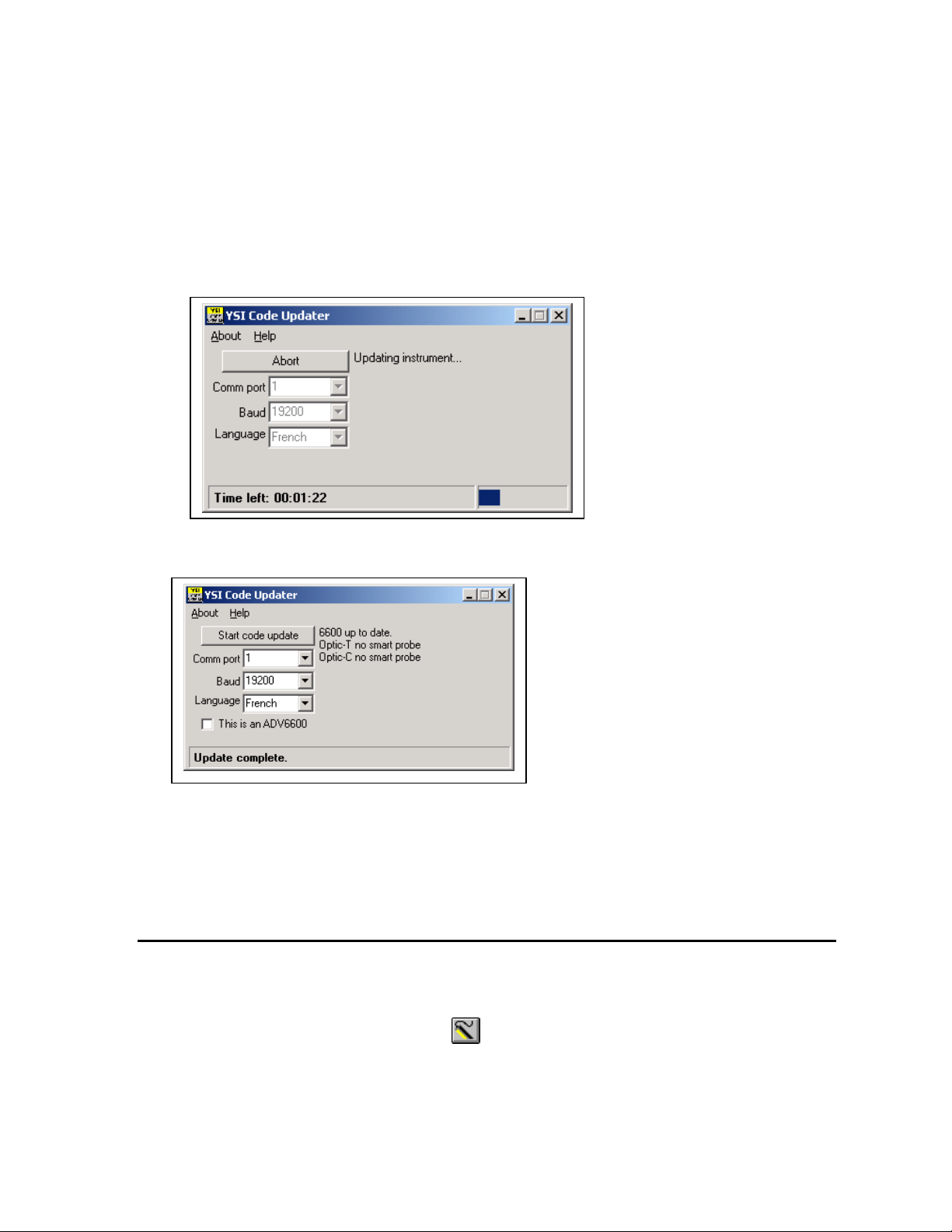
 Run the YSI Code Updater software that you just installed on your computer. The following window

will be displayed:

YSI Incorporated Environmental Monitoring Systems Operations Manual 2-25

Sondes Section 2

 Set the Comm port number to match the port to which you connected the sonde cable and make sure

that the “This is an ADV6600” selection is NOT checked.

 NEXT, SELECT THE LANGUAGE (ENGLISH, FRENCH, OR GERMAN) WHICH WILL BE

USED IN YOUR SONDE MENUS.

 Then click on the Start Code Update button. An indicator bar will show the progress of the upgrade as

shown below.

 When the update is finished (indicated on the PC screen as shown below), close the YSI Code Updater

window (on the PC) by clicking on the "X" in the upper right corner of the window.

Your sonde menus will now appear in the language which you selected prior to running the updater. If you want to change the language associated with your sonde menu, you MUST rerun the YSI Code Updater and select the new language via this mechanism.

INTERFACING TO THE SONDE WITH ECOWATCH FOR WINDOWS

When you select Sonde from the EcoWatch for Windows menus, the PC-based software begins direct communication with the sonde-based software via standard VT100 terminal emulation.

In EcoWatch for Windows, select the sonde icon, . Then select the proper Com port and confirm by clicking OK. A window similar to that shown below will appear indicating connection to the sonde as shown in Figure 39. Type “Menu” after the # sign, press Enter, and the sonde Main menu will be displayed.

YSI Incorporated Environmental Monitoring Systems Operations Manual 2-26

Sondes Section 2

------------------Main----------------1-Run 5-System 2-Calibrate 6-Report 3-File 7-Sensor 4-Status 8-Advanced

Select option (0 for previous menu):

Figure 39

If your sonde has previously been used, the Main menu (rather than the # sign) may appear when communication is established. In this case simply proceed as described below. You will not be required to type “Menu”.

If you are unable to establish interaction with the sonde, make sure that the cable is properly connected. If you are using external power, make certain that the YSI 6651 or 6038 power supply or other 12 vdc source is properly working. Recheck the setup of the Com port and other software parameters. Also refer to Section 6, Troubleshooting.

The sonde software is menu-driven. You select functions by typing their corresponding numbers. You do not need to press Enter after choosing a selection. Type the 0 or Esc key to return to the previous menu.

Sonde Main Menu

YSI Incorporated Environmental Monitoring Systems Operations Manual 2-27

Sondes Section 2

2. Upload

Sonde

SONDE MENU FLOW CHART

2. Unattended sample

1. Conductivity

2. DO %

1. Run

3. File

2. Calibrate

6. Report

7. Sensor

8. Advanced

1. Discrete sample

3. DO mg/L

2. () Time

3. () Temp, C

4. ( ) Temp, F

1. () Date

2. () Cond

3. () DO

4. ( ) ISE1 pH

1. () Temp

4. Others

2. Comm Setup

3. Page Length

4. Instrument ID

5. System

1. Date & Time

5. SDI-12 Address

3. Quick Upload

4. View File

1. Directory

5. Quick View File

6. Delete All Files

7. Test Memory

1. Cal Constants

2. Setup

3. Sensor

4. Data Filter

4. Status

Available Memory

Logging Status

Battery Voltage

Date and Time

Figure 40 - Sonde Menu Flow Chart

SYSTEM SETUP

At the Main menu, select System. The System Setup menu will be displayed.

System Setup Menu

1-Date & time 2-Comm setup 3-Page length=25 4-Instrument ID=YSI Sonde 5-Circuit board SN:00003001 6-GLP filename=00003001 7-SDI-12 address=0

Select option (0 for previous menu):

YSI Incorporated Environmental Monitoring Systems Operations Manual 2-28

Sondes Section 2

------------------Main----------------1-Run 5-System 2-Calibrate 6-Report 3-File 7-Sensor 4-Status 8-Advanced

Select option (0 for previous menu):

Select 1-Date & time. An asterisk will appear next to each selection to confirm the entry. Press 4 and 5 to activate the date and time functions. Pay particular attention to the date format that you have chosen when entering date. You must use the 24-hour clock format for entering time. Option 4- ( ) 4 digit year may be used so that the date will appear with either a two or four digit year display. If you do not enter the correct year format (8/30/98 for 2-digit, 8/30/1998 for 4 digit) your entry will be rejected.

-----------Date & time setup----------1-(*)m/d/y 4-( )4 digit year 2-( )d/m/y 5-Date=08/30/98 3-( )y/m/d 6-Time=11:12:30

Select option (0 for previous menu):

Select 4-Instrument ID from the System setup menu to record the instrument ID number (usually the instrument serial number), and press Enter. A prompt will appear which will allow you to type in the serial number of your sonde. This will make sure that any data that is collected is associated with a particular sonde. Note that the selection 5-Circuit Board SN shows the serial number of the PCB that is resident in your sonde (not the entire system as for Instrument ID). Unlike the Instrument ID, the user cannot change the Circuit Board SN. The 6-GLP filename and 7-SDI-12 address selections will be explained in Section 2.9.5

Press Esc or 0 to return to the System setup menu.

Then press Esc or 0 again to return to the Main menu.

YSI Incorporated Environmental Monitoring Systems Operations Manual 2-29

Sondes Section 2

------------Sensors enabled-----------1-(*)Time 2-(*)Temperature 3-(*)Conductivity 4-(*)Dissolved Oxy 5-(*)ISE1 pH 6-(*)ISE2 Orp 7-(*)ISE3 NH4+ 8-(*)ISE4 NO39-( )ISE5 NONE A-(*)Optic T Turbidity - 6136 B-(*)Optic C Chlorophyll

Select option (0 for previous menu):

ENABLING SENSORS

To activate the sensors that are in your sonde, select Sensor from the Sonde Main menu.

Note that the exact appearance of this menu will vary depending upon the sensors that are available on your sonde. Enter the corresponding number to enable the sensors that are installed on your sonde. An asterisk indicates that the sensor is enabled.

When selecting any of the ISE or Optical ports, a submenu will appear. When this occurs, make a selection so that the sensor corresponds to the port in which the sensor is physically installed. Only ORP can be enabled as ISE2. Optic T, Optic C, Optic B, and Optic O generate a submenu on selection. Each optical port can have one of six probes (6136 Turbidity, 6025 Chlorophyll, 6130 Rhodamine WT, 6131 BGA-PC, 6132 BGA-PE, or 6150 ROX Optical DO) installed as indicated by the submenus.

NOTE CAREFULLY: It is NOT possible to simultaneously activate BOTH the 6562 Rapid Pulse polarographic dissolved oxygen sensor and the 6150 ROX Optical dissolved oxygen sensor. Activation of either sensor will automatically deactivate the other selection. Thus, users of 6600V2-2, 6600EDS V2-2, 6820V2-1, and 6920V2-1 sondes CANNOT measure oxygen with both types of sensors.

After all installed sensors have been enabled, press Esc or 0 to return to the Main Menu.

ENABLING PARAMETERS

In order for a specific parameter to be displayed:

1. The sensor must first be enabled as described above.

2. That parameter must be activated in the Report Setup menu described below.

Select Report from the Main menu. A Report Setup menu similar to the one shown below will be displayed.

YSI Incorporated Environmental Monitoring Systems Operations Manual 2-30

Sondes Section 2

--------------Report setup------------1-(*)Date m/d/y E-(*)Orp mV 2-(*)Time hh:mm:ss F-(*)NH4+ N mg/L 3-(*)Temp C G-( )NH4+ N mV 4-(*)SpCond mS/cm H-( )NH3 N mg/L 5-( )Cond I-(*)NO3- N mg/L 6-( )Resist J-( )NO3- N mV 7-( )TDS K-(*)Cl- mg/L 8-( )Sal ppt L-( )Cl- mV 9-(*)DOsat % M-(*)Turbid+ NTU A-(*)DO mg/L N-(*)Chl ug/L B-( )DOchrg O-(*)Chl RFU C-(*)pH P-(*)Battery volts D-( )pH mV

Select option (0 for previous menu):

Note that the exact appearance of this menu will vary depending upon the sensors that are available and enabled on your sonde. The asterisks (*) that follow the numbers or letters indicate that the parameter will appear on all outputs and reports. To turn a parameter on or off, type the number or letter that corresponds to the parameter.

Note also that since a 6136 turbidity probe was selected in the Sensor menu above, the units of turbidity are presented as “turbid+ NTU”. If a 6026 turbidity probe (which was offered by YSI up until 2002) had been selected, the units of turbidity would be presented as “turbid NTU”. This designation is designed to differentiate the data from the two sensor types in later analysis.

For parameters with multiple unit options such as temperature, conductivity, specific conductance, resistivity and TDS, a submenu will appear as shown below for temperature, allowing selection of desired units for this parameter.

--------------Select units------------1-(*)NONE 2-( )Temp C 3-( )Temp F 4-( )Temp K

Select option (0 for previous menu): 2

After configuring your display with the desired parameters, press Esc or 0 to return to the Main menu.

YSI Incorporated Environmental Monitoring Systems Operations Manual 2-31

Sondes Section 2

----------------Advanced-------------1-Cal constants 2-Setup 3-Sensor 4-Data filter

Select option (0 for previous menu):

-------------Advanced setup----------1-(*)VT100 emulation 2-( )Power up to Menu 3-( )Power up to Run 4-( )Comma radix 5-(*)Auto sleep RS232 6-(*)Auto sleep SDI12 7-( )Multi SDI12 8-( )Full SDI12

Select option (0 for previous menu): 0

CHECKING ADVANCED SETTINGS

Select Advanced from the Main menu. The following menu will be displayed.

Select Setup from the Advanced menu.

Make sure that, other than Auto sleep RS232, all entries are activated or deactivated as shown above.

For sondes which will be used in sampling studies where the user is present and observes readings in realtime, Auto sleep RS232 should usually be “off‟. For sondes that will be used in unattended monitoring studies, Auto sleep RS232 should usually be “on”. This is described in detail in Section 2.9, Sonde Menu. When this setup is verified, press Esc or 0 to return to the Advanced menu.

Select 3-Sensor from the Advanced menu and make certain that the entries are identical to those shown below.

YSI Incorporated Environmental Monitoring Systems Operations Manual 2-32

Sondes Section 2

------------Advanced sensor----------1-TDS constant=0.65 2-Latitude=40 3-Altitude Ft=0 4-(*)Fixed probe 5-( )Moving probe 6-DO temp co %/C=1.1 7-DO warm up sec=40 8-( )Wait for DO 9-Wipes=1 A-Wipe int=5 B-SDI12-M/wipe=1 C-Turb temp co %/C=0.3 D-(*)Turb spike filter E-Chl temp co %/C=0 F-( )Chl spike filter

Select option (0 for previous menu):

------------------Main----------------1-Run 5-System 2-Calibrate 6-Report 3-File 7-Sensor 4-Status 8-Advanced

Select option (0 for previous menu):

If you have a depth sensor installed, you can maintain the default settings of 40 and 0 for 2-Latitude and 3-Altitude, respectively, without affecting your ability to learn the basic calibration and operation of the

sonde. However, if you know the appropriate values for your location, change them. When this setup is verified, press Esc or 0 to return to the Advanced menu. For more information, see Section 2.9.8, Advanced.

The display under 3-Sensor may be different from the one shown in the example above, depending on the sensors that are installed in your unit. For example, if you do not have a chlorophyll probe, the last two entries (which are relevant only to chlorophyll) will not appear.

When this setup is verified, press Esc or 0 to return to the Advanced menu. For a detailed explanation of the choices in the Advanced menu, see Section 2.9.8, Advanced. Press Esc or 0 to back up to the Main menu.

The sonde software is now set up and ready to calibrate and run.

YSI Incorporated Environmental Monitoring Systems Operations Manual 2-33

Sondes Section 2

2.6 GETTING READY TO CALIBRATE

2.6.1 INTRODUCTION

HEALTH AND SAFETY

Reagents that are used to calibrate and check this instrument may be hazardous to your health. Take a moment to review health and safety information in Appendix A of this manual. Some calibration standard solutions may require special handling.

CONTAINERS NEEDED TO CALIBRATE A SONDE

The calibration cup that comes with your sonde serves as a calibration chamber for all calibrations and minimizes the volume of calibration reagents required.

Although not recommended except in unusual circumstances, instead of the calibration cup, you may use laboratory glassware to perform some of the calibrations. If you do not use a calibration cup that is designed for the sonde, you are cautioned to do the following:

 Perform all calibrations with the Probe Guard installed. This protects the probes from possible physical

damage.

 Use a ring stand and clamp to secure the sonde body to prevent the sonde from falling over. Much

laboratory glassware has convex bottoms.

 Insure that all sensors are immersed in calibration solutions. Many of the calibrations factor in

readings from other probes (e.g., temperature probe). The top vent hole of the conductivity sensor must also be immersed during calibrations.

CALIBRATION TIPS

1. If you use the Calibration Cup for calibration of either the Rapid Pulse Polarographic or ROX Optical DO sensors in water-saturated air, make certain to loosen the seal to allow pressure equilibration before calibration.

2. If you choose to calibrate your Rapid Pulse Polarographic or ROX Optical

DO sensor in air-saturated water in a separate vessel, be sure to sparge the water with an aquarium pump and air-stone for at least 1 hour to assure that the water is truly saturated with air.

3. The key to successful calibration is to insure that the sensors are completely submersed when calibration values are entered. Use recommended volumes when performing calibrations.

4. For maximum accuracy, use a small amount of previously used calibration solution to pre-rinse the sonde. You may wish to save old calibration standards for this purpose.

5. Fill a bucket with ambient temperature water to rinse the sonde between calibration solutions or perform the calibration near a sink where the probes can be rinsed from the tap.

YSI Incorporated Environmental Monitoring Systems Operations Manual 2-34

Sondes Section 2

6. Have several clean, absorbent paper towels or cotton cloths available to dry the sonde between rinses and calibration solutions. Shake the excess rinse water off of the sonde, especially when the probe guard is installed. Dry off the outside of the sonde and probe guard. Making sure that the sonde is dry reduces carry-over contamination of calibrator solutions and increases the accuracy of the calibration.

7. Make certain that port plugs are installed in all ports where probes are not installed. It is extremely important to keep these electrical connectors dry.

USING THE CALIBRATION CUP

Follow these instructions to use the calibration cup for calibration procedures with all of the instruments except the 600R, 600QS, and 600 OMS V2-1. For these sondes, the over-the-guard bottle that comes with your sonde, must be used.

 Ensure that a gasket is installed in the gasket groove of the calibration cup bottom cap, and that the

bottom cap is securely tightened. Note: Do not over-tighten as this could cause damage to the threaded portions of the bottom cap and tube.

 Remove the probe guard, if it is installed.

 Inspect the installed gasket on the sonde for obvious defects and if necessary, replace it with the extra

gasket supplied.

 Screw the cup assembly into place on the threaded end of sonde and securely tighten. Note: Do not

over tighten as this could cause damage to the threaded portions of the bottom cap and tube.

 Sonde calibration can be accomplished with the sonde upright– i.e. the cable connector end of the

sonde is oriented above the probe end, or inverted where the orientation is reversed. A separate clamp and stand, such as a ring stand, is required to support the sonde in the inverted position.

 When using the Calibration Cup for dissolved oxygen calibration in water-saturated air, make certain

that the vessel is vented to the atmosphere by loosening the bottom cap or cup assembly, depending on orientation, and that approximately 1/8” of water is present in the cup.

NOTE CAREFULLY: If you are calibrating a 6136 turbidity sensor for use with a 6820V2-1 or 6920V2-1, you can use either the calibration cup supplied with your sonde or an optional extended length cup for the calibration. Please see the section below which describes the special calibration recommendations for this sensor.

YSI Incorporated Environmental Monitoring Systems Operations Manual 2-35

Sondes Section 2

Probe to Calibrate

Upright

Inverted

Conductivity

200ml

150ml

pH/ORP

125ml

175ml

ISE

125ml

175ml

All Optical Sensors

50ml

DO NOT CALIBRATE***

Probe to Calibrate

Upright

Inverted

Conductivity

320ml

150ml

pH/ORP

240ml

175ml

ISE

240ml

175ml

All Optical Sensors

225ml

DO NOT CALIBRATE***

Probe to Calibrate

Upright

Inverted

Conductivity

310ml

150ml

pH/ORP

200ml

150ml

ISE

200ml

150ml

All Optical Sensors

225 ml

DO NOT CALIBRATE***

Probe to Calibrate

Upright

Inverted

Conductivity

50ml

pH/ORP

25ml

50ml

Probe to Calibrate

Upright

Inverted

Conductivity

425ml (650ml)

250ml (250ml)

pH/ORP

300ml (500ml)

250ml (250ml))

ISE

300ml (500ml)

250ml (250ml)

All Optical Sensors

180ml (500ml)

DO NOT CALIBRATE***

Probe to Calibrate

Upright

Inverted

Conductivity

275ml (520ml)

350ml (350ml)

pH/ORP

175ml (400ml)

350ml (350ml)

All Optical Sensors

225ml (420ml)

DO NOT CALIBRATE***

RECOMMENDED VOLUMES OF CALIBRATION REAGENTS

The approximate volumes of the reagents are specified below for both the upright and inverted orientations. Note that the volume values are only estimates. The actual amount of calibrator solution required will depend on how many and what type of other probes are installed in you sonde bulkhead.

Table 1A 6820V2-1 and 6920V2-1 Sondes with Standard Calibration Cup*

Table 1B 6820V2-1 and 6920V2-1 Sondes with Optional Extended Calibration Cup*

Table 2 6820V2-2 and 6920V2-2 Sondes with Extended Calibration Cup*

Table 3 600XL and 600XLM Sondes

Table 4 6600V2-2 Sonde with Short Calibration Cup and Long Cup in Parentheses*

Table 5 6600EDSV2-2 Sonde with Short Calibration Cup and Long Cup in Parentheses*

YSI Incorporated Environmental Monitoring Systems Operations Manual 2-36

Sondes Section 2

Probe to Calibrate

Upright

Inverted

Conductivity

525ml

150ml

pH/ORP

500ml

150ml

All Optical Sensors

425ml

DO NOT CALIBRATE***

Probe to Calibrate

Upright

Inverted

Conductivity

375ml

N/A

Turbidity, Chlorophyll, Rhodamine WT

350ml

N/A

Probe to Calibrate

Upright

Inverted

Conductivity

350ml

N/A

pH/ORP

120ml

N/A

Table 6 6600V2-4 Sonde with Standard Long Calibration Cup****

Table 7 600 OMS V2-1 Sonde* *

Table 8 600R and 600QS Sondes

* See section below for special instructions dealing with calibration of 6136 turbidity sensor.

** See section below for special instructions dealing with calibration of the conductivity sensor for the 600 OMS V2-1.

*** Optical Sensors CANNOT be calibrated with the sonde in the Upside-Down position because of interference from the meniscus of the calibration standard.

**** An extended length calibration cup is supplied with the 6600V2-4, 6600V2-2, and 6600EDSV2-2 to facilitate calibration of the 6136 turbidity sensor. This cup requires the use of larger volumes of other calibration solutions. Users may choose to purchase the shorter calibration cup sleeve for calibration of sensors other than the 6136 to reduce the volumes of calibrant. The shorter cal cup sleeve is YSI Item Number 066267 and can be obtained by contacting YSI Technical Support.

CALIBRATION OF THE 6136 TURBIDITY SENSOR

The 6136 can be calibrated using either the calibration cup supplied with the sonde or with an extended length calibration cup which can be purchased as an option for the 6820V2-1 and 6920V2-1. An extended cup is supplied as a standard item with the 6820V2-2, 6920V2-2, 6600V2-4, 6600V2-2, and 6600EDSV2-2 sondes. If you choose to calibrate with the short calibration cup, you also MUST first make certain that the vessel is equipped with a BLACK bottom. In addition, you should engage only ONE THREAD when screwing the calibration cup onto the sonde in order to keep the turbidity probe face as far as possible from the calibration cup bottom to avoid interference. Even with these techniques, there will still be a small interference from the bottom of the calibration cup that will cause your field turbidity readings to be approximately 0.5 NTU lower than the actual reading. This small error is usually only evident when the sonde is deployed in very clear water where the readings might appear as slightly negative values, e.g., a turbidity of 0.1 NTU would appear as –0.4 NTU.

Use of the extended length cup will require the use of significantly more standard solutions for 6820V2-1/ 6920V2-1 sondes (additional 180 mL) if calibration is done in the upright position. To minimize calibration solution volumes for sensors other than turbidity, users may wish to purchase the shorter calibration cup sleeve which is supplied as standard with the 6820V2-1 and 6920V2-1. The shorter cal cup sleeve for any 6600 is Item Number 066267, and the shorter cal cup sleeve for any 6820/6920 is Item Number 069286. These can be ordered from YSI Technical Support.

YSI Incorporated Environmental Monitoring Systems Operations Manual 2-37

Sondes Section 2

---------------Calibrate-------------1-Conductivity 6-ISE3 NH4+ 2-Dissolved Oxy 7-ISE4 NO3- 3-Pressure-Abs 8-Optic T-Turbidity-6026 4-ISE1 pH 9-Optic C-Chlorophyll 5-ISE2 ORP

Select option (0 for previous menu):

NOTE CAREFULLY: All optical sensors MUST be calibrated in the upright position no matter which type of calibration cup is employed. In the upside-down position, the meniscus of the standard causes a great deal of interference and this interference is likely to result in calibration errors and/or erroneous field readings.

CALIBRATION OF 600 OMS V2-1 CONDUCTIVITY SENSOR

In order to conserve calibration solution, the 600 OMS V2-1conductivity sensor should be calibrated with the optical probe removed and the optical port plug securely tightened. The volume of conductivity solution provided in Table 7 above reflects this special condition. In addition, it is recommended that the sonde be shaken vigorously after immersion in the conductivity reagent to assure that bubbles are expelled from the cell.

An instruction sheet dealing in greater detail with the special requirements for calibration of 600 OMS V21sensors is included with the sonde. Be sure to read the instructions carefully before using the sonde.

2.6.2 CALIBRATION PROCEDURES

The following calibration procedures are the most commonly used methods for the 6-series sensors. For detailed information on all calibration procedures, refer to Section 2.9.2, Calibrate.

To ensure more accurate results, you can rinse the calibration cup with water, and then rinse with a small amount of the calibration solution for the sensor that you are going to calibrate. Discard the rinse solution and add fresh calibrator solution. Use tables 1-8 to find the correct amount of calibrator solution.

1. Carefully immerse the probes into the solution and rotate the calibration cup to engage several

threads. YSI recommends supporting the sonde with a ring stand and clamp to prevent the sonde from falling over.

2. With the proper cable, connect the sonde to a PC, access EcoWatch for Windows and proceed to

the Main menu (for information on how to run EcoWatch for Windows software, see Section

2.4.2, Running EcoWatch Software). From the sonde Main menu, select 2-Calibrate.

YSI Incorporated Environmental Monitoring Systems Operations Manual 2-38

Sondes Section 2

------------Cond calibration----------1-SpCond 2-Cond 3-Salinity

Select option (0 for previous menu): 1

Enter SpCond in mS/cm (10):

Date Time Temp SpCond Cond Sal DOsat DO Depth pH Battery mm/dd/yy hh:mm:ss C mS/cm mS/cm ppt % mg/L feet volts

-----------------------------------------------------------------------------To calibrate, press <Enter> when the readings are stable.

05/05/97 08:39:51 20.83 9.602 8.837 5.41 37.9 3.28 -0.252 7.06 10.2

3. Note that the exact appearance of this menu will vary depending upon the sensors that are available and enabled on your sonde. To select any of the parameters from the Calibrate menu, input the number that is next to the parameter. Once you have chosen a parameter, some of the parameters will have a number that appears in parentheses. These are the default values and will be used during calibration if you press Enter without inputting another value. Be sure not to accept default values unless you have assured that they are correct. If no default value appears, you must type a numerical value and press Enter.

4. After you input the calibration value, or accept the default, press Enter. A real-time display will appear on the screen. Carefully observe the stabilization of the readings of the parameter that is being calibrated. When the readings have been stable for approximately 30 seconds, press Enter to accept the calibration. The calibrated value is bolded on the example screen on the following page.

5. Press Enter to return to the Calibrate menu, and proceed to the next calibration.

CALIBRATION EXAMPLE

The example below for calibration of specific conductance, is designed to demonstrate the general calibration protocol for all parameters. From the Calibrate menu, press 1-Conductivity and the following display will be shown.

Select 1-SpCond (the generally-recommended method for calibration of a conductivity sensor) and the following prompt will appear which calls for your numerical input of the specific conductance of your calibration solution.

As noted above, the number in parentheses is the default value of this parameter and will be used in the

calibration if only Enter is pressed without typing in another value. Similar prompts will be displayed during

the calibration of all parameters, but for some sensors, such as pH, no default values are provided. In these cases, the user must input a numerical value and then press Enter.

After the correct calibration value for your solution is input and Enter is pressed, a real-time display similar to the following will then appear on the screen..

YSI Incorporated Environmental Monitoring Systems Operations Manual 2-39

Sondes Section 2

Calibrated. Press <Enter> to continue.

Note that all parameters that have been enabled will appear - not just the one being calibrated at the moment. The user should carefully observe the stabilization of the readings of the parameter that is being calibrated and, when the readings are stable for approximately 30 seconds, press Enter to implement the calibration and the following message will appear.

NOTE: If an ERROR message appears, begin the calibration procedure again. Be certain that the value you enter for the calibration standard is correct. Also see Section 6, Troubleshooting for more information on error messages.

CAUTION: Be certain to immerse the entire sonde in solution standards for calibration of all parameters. Most calibrations require readings not only from the sensor being calibrated but also from the temperature sensor.

Specific start-up calibration procedures for all sensors that commonly require calibration are provided in the following paragraphs of this section. Remember that these are basic protocols designed to get the user up and running with your 6-series sonde. A more-detailed discussion of sensor calibration can be found in Section

2.9.2.

CONDUCTIVITY

This procedure calibrates conductivity, specific conductance, salinity, and total dissolved solids.

Place the correct amount (see Tables 1-8) of 10 mS/cm conductivity standard (YSI 3163 is recommended) into a clean, dry or pre-rinsed calibration cup.

Before proceeding, ensure that the sensor is as dry as possible. Ideally, rinse the conductivity sensor with a small amount of standard that can be discarded. Be certain that you avoid cross-contamination of standard solutions with other solutions. Make certain that there are no salt deposits around the oxygen and pH/ORP probes, particularly if you are employing standards of low conductivity.

Carefully immerse the probe end of the sonde into the solution. Gently rotate and/or move the sonde up

and down to remove any bubbles from the conductivity cell. The probe must be completely immersed past its vent hole. Using the recommended volumes from the table in the previous subsection should insure that the vent hole is covered.

Allow at least one minute for temperature equilibration before proceeding.

From the Calibrate menu, select Conductivity to access the Conductivity calibration procedure and then 1- SpCond to access the specific conductance calibration procedure. Enter the calibration value of the standard you are using (mS/cm at 25C) and press Enter. The current values of all enabled sensors will appear on the screen and will change with time as they stabilize.

Observe the readings under Specific Conductance or Conductivity and when they show no significant change for approximately 30 seconds, press Enter. The screen will indicate that the calibration has been accepted and prompt you to press Enter again to return to the Calibrate menu.

Rinse the sonde in tap or purified water and dry the sonde.

YSI Incorporated Environmental Monitoring Systems Operations Manual 2-40

Sondes Section 2

NOTE: The YSI conductivity system is very linear over its entire 0-100 mS/cm range. Therefore, it is usually not necessary to use calibration solutions other than the 10 mS/cm reagent recommended above for all environmental applications from low conductivity freshwater to seawater. YSI does offer the 3161 (1 mS/cm) and 3165 (100 mS/cm) conductivity standards for users who want to assure maximum accuracy at the high and low ends of the sensor range. Users of the 1 mS/cm standard should be particularly careful to avoid contamination of the reagent. In fact, because of contamination issues, YSI does not recommend using standards less than 1 mS/cm.

NOTE: For calibration of the 600 OMS V2-1conductivity sensor, the optical probe must be removed and the port plugged. See specific instructions in the application note supplied with the 600 OMS V2-1.

RAPID PULSE POLAROGRAPHIC DISSOLVED OXYGEN

Place approximately 3 mm (1/8 inch) of water in the bottom of the calibration cup. Place the probe end of the sonde into the cup. Make certain that the DO and temperature probes are not immersed in the water. Engage only 1 or 2 threads of the calibration cup to insure the DO probe is vented to the atmosphere. Wait approximately 10 minutes for the air in the calibration cup to become water saturated and for the temperature to equilibrate.

Two calibration protocols are provided below for Rapid Pulse dissolved oxygen, one for sampling applications and one for long-term monitoring applications.

Sampling Applications

If your instrument will be used in sampling applications where the dissolved oxygen is “on” continuously during the study, deactivate “Autosleep RS232” as described in Section 2.5, Sonde Software Setup.

From the Calibrate menu, select Dissolved Oxy, then 1-DO % to access the DO percent calibration procedure. Calibration of dissolved oxygen in the DO % procedure also results in calibration of the DO mg/L mode and vice versa.

Enter the current barometric pressure in mm of Hg. (Inches of Hg x 25.4 = mm Hg).

Note: Laboratory barometer readings are usually “true” (uncorrected) values of air pressure and can be used

“as is” for oxygen calibration. Weather service readings are usually not “true”, i.e., they are corrected to sea level, and therefore cannot be used until they are “uncorrected”. An approximate formula for this “uncorrection” (where the BP readings MUST be in mm Hg) is:

True BP = [Corrected BP] – [2.5 * (Local Altitude in feet above sea level/100)]

Press Enter and the current values of all enabled sensors will appear on the screen and change with time as they stabilize. Observe the readings under DO%. When they show no significant change for approximately 30 seconds, press Enter. The screen will indicate that the calibration has been accepted and prompt you to press Enter again to return to the Calibrate menu.

Rinse the sonde in water and dry the sonde.

YSI Incorporated Environmental Monitoring Systems Operations Manual 2-41

Sondes Section 2

=================================================================== Temp SpCond Sal DOsat DO Depth pH NH4+ N NO3- N Turbid C mS/cm ppt % mg/L feet mg/L mg/L NTU

------------------------------------------------------------------Stabilizing: 38

Monitoring Applications

If your instrument will be used in monitoring applications where data is being captured at a longer interval (e.g. 15 – 60 minutes) to internal sonde memory, a data collection platform or a computer, you need to activate “Autosleep RS232” as described in Section 2.5, Sonde Software Setup. Then follow the instructions detailed above for the Sampling Application calibration. With Autosleep active, the calibration will occur automatically with a display similar to that shown below.

After the warm-up time is complete, the readings just before and just after calibration are displayed. When you press Enter, the screen returns to the DO Calibration menu.

ROX OPTICAL DISSOLVED OXYGEN

Place the sensor either (a) into a calibration cup containing about 1/8 inch of water which is vented by loosening the threads or (b) into a container of water which is being continuously sparged with an aquarium pump and air stone. Wait approximately 10 minutes before proceeding to allow the temperature and oxygen pressure to equilibrate.

Select ODOsat % and then 1-Point to access the DO calibration procedure. Calibration of your Optical dissolved oxygen sensor in the DO % procedure also results in calibration of the DO mg/L mode and vice versa.

Enter the current barometric pressure in mm of Hg. (Inches of Hg x 25.4 = mm Hg).

Note: Laboratory barometer readings are usually “true” (uncorrected) values of air pressure and can be used

True BP = [Corrected BP] – [2.5 * (Local Altitude in ft above sea level/100)]

Press Enter and the current values of all enabled sensors will appear on the screen and change with time as they stabilize. Observe the readings under ODOsat %. When they show no significant change for approximately 30 seconds, press Enter. The screen will indicate that the calibration has been accepted and prompt you to press Enter again to return to the Calibrate menu.

The minor advantages and disadvantages of calibration in air-saturated water versus water-saturated air are outlined in Appendix M, ROX Optical DO Sensor

NOTE CAREFULLY: As opposed to the 6562 Rapid Pulse Polarographic DO sensor described above, there is no difference between the calibration routine for sensors which will be used for sampling or monitoring applications. Usually the Autosleep RS-232 feature in the Advanced|Setup menu will be activated for ROX calibrations, but there is no problem if it is not active.

Rinse the sonde in water and dry the sonde.

YSI Incorporated Environmental Monitoring Systems Operations Manual 2-42

Sondes Section 2

DEPTH AND LEVEL

For the depth and level calibration, make certain that the depth sensor module is in air and not immersed in any solution.

From the Calibrate menu, select Pressure-Abs (or Pressure-Gage if you have a vented level sensor) to access the depth calibration procedure. Input 0.00 or some known sensor offset in feet. Press Enter and monitor the stabilization of the depth readings with time. When no significant change occurs for approximately 30 seconds, press Enter to confirm the calibration. This zeros the sensor with regard to current barometric pressure. Then press Enter again to return to the Calibrate menu.

For best performance of depth measurements, users should ensure that the sonde‟s orientation remains constant while taking readings. This is especially important for vented level measurements and for sondes with side mounted pressure sensors.

pH 2-POINT

Using the correct amount of pH 7 buffer standard (see Tables 1-8) in a clean, dry or pre-rinsed calibration cup, carefully immerse the probe end of the sonde into the solution. Allow at least 1 minute for temperature equilibration before proceeding.

From the Calibrate menu, select ISE1 pH to access the pH calibration choices and then press 2- 2-Point. Press Enter and input the value of the buffer at the prompt.

NOTE: The actual pH value of all buffers is somewhat variable with temperature and that the correct value from the bottle label for your calibration temperature should be entered for maximum accuracy. For example, the pH of YSI “pH 7 Buffer” is 7.00 at 25 C, but 7.02 at 20 C.

After entering the correct pH value of the buffer, press Enter and the current values of all enabled sensors will appear on the screen and change with time as they stabilize in the solution. Observe the readings under pH and when they show no significant change for approximately 30 seconds, press Enter. The display will indicate that the calibration is accepted.

After the pH 7 calibration is complete, press Enter again, as instructed on the screen, to continue. Rinse the sonde in water and dry the sonde before proceeding to the next step.

Using the correct amount (see Tables 1-8) of an additional pH buffer standard into a clean, dry or prerinsed calibration cup, carefully immerse the probe end of the sonde into the solution. Allow at least 1 minute for temperature equilibration before proceeding.

Press Enter and input the correct value of the second buffer for your calibration temperature at the prompt. Press Enter and the current values of all enabled sensors will appear on the screen and will change with time as they stabilize in the solution. Observe the readings under pH and when they show no significant change for approximately 30 seconds, press Enter. After the second calibration point is complete, press Enter again, as instructed on the screen, to return to the Calibrate menu.

Rinse the sonde in water and dry. Thoroughly rinse and dry the calibration containers for future use.

NOTE: The majority of environmental water of all types has a pH between 7 and 10. Therefore, unless you anticipate a pH of less than 7 for your application, YSI recommends a two point calibration using pH 7 and pH 10 buffers.

YSI Incorporated Environmental Monitoring Systems Operations Manual 2-43

Sondes Section 2

WARNING: AMMONIUM AND NITRATE SENSORS CAN ONLY BE USED AT DEPTHS OF LESS THAN 50 FEET (15 METERS). USE OF THE SENSORS AT GREATER DEPTHS IS LIKELY TO PERMANENTLY DAMAGE THE SENSOR MEMBRANE.

The next calibration instructions are only for the ISE sensors which are options for the 6820V2-1, 6800V2-2, 6600V2-2, 6920V2-1, and 6920V2-2 sondes. If you do not have one of these sondes, you may skip to the next section.

AMMONIUM (NH

) , CHLORIDE CL- AND NITRATE (NO

The calibration procedures for ammonium, nitrate or chloride are similar to pH except for the reagents in the calibration solutions. Suggested values for calibrants are 1 and 100 mg/L of either ammonium-nitrogen (NH4-N) or nitrate-nitrogen (NO3-N). Suggested values for calibrants are 10 and 1000 mg/L of Chloride (Cl-).

NOTE: The following procedure requires one portion of the high concentration calibrant and two portions of the low concentration calibrant. The high concentration solution and one of the low concentration solutions should be at ambient temperature. The other low concentration solution should be chilled to less than 10C prior to beginning the procedure.

Place the proper amount of 100 mg/L standard (1000mg/l for chloride) into a clean, dry or pre-rinsed transport cup. Carefully immerse the probe end of the sonde into the solution. Allow at least 1 minute for temperature equilibration before proceeding.

Select Ammonium, Nitrate, or Chloride to access the appropriate calibration choices. Then select 3-3- Point. Press Enter and input the concentration value of the standard as requested. Press Enter and the current values of all enabled sensors will appear on the screen and will change with time as they stabilize in the solution. Observe the readings under NH4+, NO3-, or Cl- . When they show no significant change for approximately 30 seconds, press Enter.

After the first calibration point is complete, proceed as instructed on the screen, to continue. Rinse the sonde in water and dry the sonde prior to the next step.

Place the proper amount of 1 mg/L standard for Ammonium or Nitrate (10 mg/l for Chloride) into a clean, dry or pre-rinsed transport cup. Carefully immerse the probe end of the sonde into the solution. Allow at least 1 minute for temperature equilibration before proceeding.

Press Enter and input the concentration value of the standard as requested.

Press Enter and the current values of all enabled sensors will appear on the screen and will change with time as they stabilize in the solution. Observe the readings under NH4+, NO3-, or Cl-.and when they have show no significant change for approximately 30 seconds, press Enter.

After the second value calibration is complete, press Enter to continue. Place the proper amount of chilled 1 mg/L standard (10 mg/L for the chloride) into a clean, dry or pre-rinsed calibration cup. Carefully immerse the probe end of the sonde into the solution. Allow at least 5 minutes for temperature equilibration before proceeding.

Press Enter and input the concentration value of the standard as requested. Press Enter and the current values of all enabled sensors will appear on the screen and will change with time as they stabilize in the solution. Observe the readings under NH4+, NO3-. or Cl-. and when they show no significant change for approximately 30 seconds, press Enter. After the third value calibration is complete, press Enter to return to the Calibrate menu.

Thoroughly rinse and dry the calibration cups for future use.

) 3-POINT

YSI Incorporated Environmental Monitoring Systems Operations Manual 2-44

Sondes Section 2

CALIBRATION TIP: Exposure to the high ionic content of pH buffers can cause a significant, but temporary, drift in these ISE probes (ammonium, nitrate and chloride probes). Therefore, when calibrating the pH probe, YSI recommends that you use one of the following methods to minimize errors in the subsequent readings:

 Calibrate pH first, immersing all of the probes in the pH buffers. After calibrating pH, place the

probes in 100 mg/L nitrate or ammonium standard or 1000 mg/L chloride standard and monitor the reading. Usually, the reading starts low and may take as long as 30 minutes to reach a stable value. When it does, proceed with the calibration.

 When calibrating pH, remove ISE modules from the sonde bulkhead and plug the ports. After pH

calibration is complete, replace the ISE sensors and proceed with their calibration with no stabilization delay.

TURBIDITY 2-POINT

Select Optic X –Turbidity-6136 or Optic X – Turbidity 6026 from the Calibrate Menu and then 2-2Point.

NOTE: Before calibrating your 6136 turbidity sensor, pay particular attention to the following cautions:

 To properly calibrate YSI turbidity sensors, you MUST use standards that have been prepared

according to details in Standard Methods for the Treatment of Water and Wastewater (Section 2130 B). Acceptable standards include (a) formazin prepared according to Standard Methods; (b) dilutions of

4000 NTU formazin concentrate purchased from Hach; (c) Hach StablCalTM standards in various NTU denominations; and (d) AMCO-AEPA standards prepared specifically for the 6026 and 6136 by either YSI or approved vendors who are listed on the YSI website (www.ysi.com). STANDARDS FROM OTHER VENDORS ARE NOT APPROVED FOR THE YSI TURBIDITY SYSTEM AND THEIR USE WILL LIKELY RESULT IN BOTH CALIBRATION ERRORS AND INCORRECT FIELD READINGS.

 For AMCO-AEPA standards, the value entered by the user during the calibration protocol is

DIFFERENT depending on which YSI turbidity sensor (Legacy 6026 or Current 6136) is being calibrated. This reflects the empirically determined fact that 6026 and 6136 sensors that have been calibrated to the same value in the primary standard formazin, will have different responses in suspensions of the AEPA-AMCO beads. This effect is likely due to the larger optical cell volume of the 6136. Thus, for example, the label of the YSI 6073 turbidity standard bottle indicates that the value of the standard is 100 NTU when used for calibration of the 6026 sensor, but 126 NTU when used to calibrate the 6136. Note that the phenomenon of a sensor-specific formazin/AEPA-AMCO ratio is well known for sensors other than the 6026 and 6136.

 When calibrating a 6136 turbidity sensor you MUST carefully follow the instructions found above in

Section 2.6.1 to avoid interference from the bottom of the calibration cup. Failure to carry out the calibration properly can result in inaccurate readings, particularly water of very low turbidity.

 Before proceeding with the calibration, be certain that the probe compartment of the sonde has been

cleaned and is free of debris. Solid particles from this source, particularly those carried over from past deployments, will contaminate the standards during your calibration protocol and cause either calibration errors and/or inaccurate field data.

 One standard must be 0 NTU, and this standard must be calibrated first.

To begin the calibration, place the correct amount (see Tables 1-8 above) of 0 NTU standard (clear deionized or distilled water) into the calibration cup provided with your sonde. Immerse the sonde in the

YSI Incorporated Environmental Monitoring Systems Operations Manual 2-45

Sondes Section 2

water. Input the value 0 NTU at the prompt, and press Enter. The screen will display real-time readings that will allow you to determine when the readings have stabilized. Activate the wiper 1-2 times by pressing 3-Clean Optics as shown on the screen, to remove any bubbles. After stabilization is complete, press Enter to “confirm” the first calibration and then, as instructed, press Enter to continue.

Dry the sonde carefully and then place the sonde in the second turbidity standard (100 or 126 NTU is suggested) using the same container as for the 0 NTU standard. Input the correct turbidity value in NTU, press Enter, and view the stabilization of the values on the screen in real-time. As above, activate the wiper with the “3” key or manually rotate the sonde to remove bubbles. After the readings have stabilized, press Enter to confirm the calibration and then press Enter to return to the Calibrate menu.

Thoroughly rinse and dry the calibration cups for future use. For additional information related to calibrating the turbidity sensor, see Appendix E, Turbidity Measurements.

CHLOROPHYLL 1-POINT

Select Optic X -Chlorophyll from the Calibrate Menu, Chl µg/L and then 1-1 point.

NOTE: This procedure will zero your fluorescence sensor and use the default sensitivity for calculation of

chlorophyll concentration in µg/L, allowing quick and easy fluorescence measurements that are only semiquantitative with regard to chlorophyll. However, the readings will reflect changes in chlorophyll from site to site, or over time at a single site.

To increase the accuracy of your chlorophyll measurements, follow the 2-point or 3-point calibration protocols outlined in Section 2.9, Sonde Menu.

Before making any field readings, carefully read Section 5.14, Chlorophyll and Appendix I, Chlorophyll Measurements that describe practical aspects of fluorescence measurements.

Thoroughly rinse and dry the calibration cups for future use. For additional information related to calibrating the chlorophyll sensor, see Section 5.14, Chlorophyll and Appendix I, Chlorophyll Measurements.

BGA-PC 1-POINT

Select Optic X BGA-PC - from the Calibrate Menu, and then 1-1 point.

NOTE: This procedure will zero your fluorescence sensor and use the default sensitivity for calculation of

phycocyanin-containing BGA in cells/mL, allowing quick and easy fluorescence measurements that are only semi-quantitative with regard to BGA-PC. However, the readings will reflect changes in BGA-PC from site to site, or over time at a single site.

To increase the accuracy of your BGA-PC measurements, follow the 2-point calibration protocols outlined in Section 2.9, Sonde Menu.

YSI Incorporated Environmental Monitoring Systems Operations Manual 2-46

Sondes Section 2

Before making any field readings, carefully read Section 5.16, Principles of Operation to better understand the practical aspects of BGA-PC fluorescence measurements.

To begin the calibration, place the correct amount (see Tables 1-8 above) of clear deionized or distilled water into the YSI clear calibration cup provided. Immerse the sonde in the water. Input the value 0 cells/mL at the prompt, and press Enter. The screen will display real-time readings that will allow you to determine when the readings have stabilized. Activate the wiper 1-2 times by pressing 3-Clean Optics as shown on the screen to remove any bubbles from the sensor. After stabilization is complete, press Enter to “confirm” the calibration and then, as instructed, press Enter to return to the Calibrate menu. Note that because the range of the BGA sensors in cells/mL is large, the readings may appear to be somewhat noisier during the calibration procedure than for other 6-series sensors. Variations of +/- 400 cells/mL for the zero point can be observed with a properly functioning sensor since this value is only 0.2% of the range.

Thoroughly rinse and dry the calibration cups for future use. For additional information related to calibrating the BGA-PC sensor, see Section 5.16, Principles of Operation.

Note that the 1-point calibration of the BGA-PC sensor in cells/mL will also zero the PC RFU (Relative Fluorescence Units) parameter which is in units of percent of the full scale of the sensor. Users may wish to activate PC RFU in the Report menu and simply use this parameter to determine BGA-PC events until a good correlation between the observed cells/mL value and the value determined from laboratory analysis has been established.

BGA-PE 1-POINT

Select Optic X BGA-PE - from the Calibrate Menu, and then 1-1 point.

NOTE: This procedure will zero your fluorescence sensor and use the default sensitivity for calculation of

phycoerythrin-containing BGA in cells/mL, allowing quick and easy fluorescence measurements that are only semi-quantitative with regard to BGA-PE. However, the readings will reflect changes in BGA-PE from site to site, or over time at a single site.

To increase the accuracy of your BGA-PE measurements, follow the 2-point calibration protocols outlined in Section 2.9, Sonde Menu.

Before making any field readings, carefully read Section 5.17, Principles of Operation to better understand the practical aspects of BGA-PE fluorescence measurements.

Thoroughly rinse and dry the calibration cups for future use. For additional information related to calibrating the BGA-PE sensor, see Section 5.17, Principles of Operation.

Note that the 1-point calibration of the BGA-PE sensor in cells/mL will also zero the PE RFU (Relative Fluorescence Units) parameter which is in units of percent of the full scale of the sensor. Users may wish to activate PC RFU in the Report menu and simply use this parameter to determine BGA-PE events until a good correlation between the observed cells/mL value and the value determined from laboratory analysis has been established.

YSI Incorporated Environmental Monitoring Systems Operations Manual 2-47

Sondes Section 2

RHODAMINE WT 2-POINT

Select Rhodamine from the Calibrate Menu and then 2-2-Point.

NOTE: One standard must be 0 ug/L in rhodamine WT, and this standard must be calibrated first.

To begin the calibration, place the correct amount (see Tables 1-8) of 0 standard (clear deionized or distilled water) into the calibration cup provided with your sonde and immerse the sonde in the water. Input the value 0 ug/L at the prompt, and press Enter. The screen will display real-time readings that will allow you to determine when the readings have stabilized. Activate the wiper 1-2 times by pressing 3- Clean Optics as shown on the screen, to remove any bubbles. After stabilization is complete, press Enter to “confirm” the first calibration and then, as instructed, press Enter to continue.

Dry the sonde carefully and then place the sonde in the second rhodamine WT standard (100 ug/L is recommended) using the same container as for the 0 ug/L standard. Input the correct rhodamine WT concentration in ug/L, press Enter, and view the stabilization of the values on the screen in real-time. As above, activate the wiper with the “3” key or manually rotate the sonde to remove bubbles. After the readings have stabilized, press Enter to confirm the calibration and then press Enter to return to the Calibrate menu.

Thoroughly rinse and dry the calibration cups for future use.

YSI Incorporated Environmental Monitoring Systems Operations Manual 2-48

Sondes Section 2

---------------Run setup--------------1-Discrete sample 2-Unattended sample

Select option (0 for previous menu): 1

------------Discrete sample-----------1-Start sampling 2-Sample interval=4 3-File= 4-Site= 5-Open file

Select option (0 for previous menu):

2.7 TAKING READINGS

After you have (1) enabled the sensors, (2) set the report to show the parameters that you want to see, and (3) calibrated the sensors, you are now ready to take readings.

There are two basic approaches to sampling, discrete and unattended. Using discrete sampling, the sonde is connected via a communication cable to a PC or 650 MDS Display/Logger. The sampling frequency is likely to be rapid (seconds) in order to obtain a representative sampling as you move from site to site. Readings will probably be logged to several different files.

Unattended sampling is normally done with sondes that have internal batteries. The sampling frequency is likely to be longer (minutes or hours). A sonde is typically deployed for days or weeks at a time, and readings will be logged to a single file. The communication cable may be disconnected and internal battery power used to operate the sonde. Alternatively, the sonde may connect via SDI-12 communication to a data collection platform (DCP). Sondes without batteries need to be connected to an external power source for unattended sampling.

Select 1-Run from the Main menu to begin taking readings or to set/verify the parameters required for a study. There are two options in the Run menu as shown below.

DISCRETE SAMPLING

Select 1-Discrete sample from the Run menu. The Discrete sample menu will be displayed.

Select 2-Sample Interval to type a number that represents the number of seconds between samples. The maximum sample interval is 32767 seconds (9+ hours). The factory default sample interval is 4 seconds and works best for most discrete sampling applications. See Section 2.9.1 for more details.

Select 3-File to enter a filename with a maximum of 8 characters. This is the file to which you will log readings.

YSI Incorporated Environmental Monitoring Systems Operations Manual 2-49

Sondes Section 2

============================================================ Temp Sal DOsat DO Depth pH NH4+ N NO3- N Turbid C ppt % mg/L feet mg/L mg/L NTU

-----------------------------------------------------------*** 1-LOG last sample 2-LOG ON/OFF, 3-Clean optics ***

23.54 0.00 96.5 8.20 1.001 5.20 0.853 0.522 0.3 *** LOG is ON, hit 2 to turn it OFF, 3-Clean optics ***

23.53 0.00 96.5 8.20 1.001 5.20 0.856 0.520 0.3

23.53 0.00 96.5 8.20 1.000 5.20 0.854 0.521 0.3

23.53 0.00 96.5 8.20 1.000 5.19 0.852 0.522 0.3 *** 1-LOG last sample 2-LOG ON/OFF, 3-Clean optics ***

23.53 0.00 96.5 8.20 1.000 5.19 0.852 0.522 0.3 Sample logged.

If you started sampling without entering a filename, the default name NONAME1 will be assigned to your file. Whenever you press 1-LOG last sample or 2-LOG ON/OFF from the menu, NONAME1 will be opened during sampling. If this happens, and you want to restart the file with a different name, press 5-Close file and rename the file.

Select 4-Site to assign a site name with a maximum of 31 characters. This allows you to enter the name of the site where you are sampling.

When you select 5-Open File, a file is opened and the number 5 changes to Close File. When you are finished logging data to the file, press 5-Close File and number 5 changes back to Open File.

Now select 1-Start sampling to start discrete sampling.

After the initial sampling time interval has passed, (e.g. 4 seconds in the example above), sequential lines of data will appear on the screen.

The following prompt will appear just below the screen header:

1-LOG last sample, 2-LOG ON/OFF, 3-Clean optics.

By entering 1–LOG last sample, a single line of data can be logged to sonde memory and the following message will be displayed: Sample logged.

By entering 2-LOG ON/OFF, a set of data can be logged to memory and the following message will be displayed: LOG is ON, hit 2 to turn it OFF, 3-Clean optics. Press 2 again to terminate logging.

By entering 3-Clean optics, if your unit has an optical probe, the wiper will clean the optical surface. The 3-Clean optics portion of the prompt will only appear if an optical probe was installed and enabled.

Select Esc or press 0 to exit discrete sampling.

UNATTENDED SAMPLING

Select 2-Unattended Sampling from the Run menu. The Unattended sample menu will be displayed. Use the following example to understand the unattended sampling option.

Example: You are going to deploy the sonde for 2 weeks, collecting a set of readings every 15 minutes. You start at 6:00 PM on July 17, 1996 and end the

YSI Incorporated Environmental Monitoring Systems Operations Manual 2-50

Sondes Section 2

------------Unattended setup----------1-Interval=00:15:00 2-Start date=07/17/96 3-Start time=18:00:00 4-Duration days=365 5-File= 6-Site= 7-Bat volts: 11.6 8-Bat life 25.1 days 9-Free mem 41.3 days A-1st sample in 8.10 minutes B-View params to log C-Start logging

sampling at 6:00 PM on July 31, 1996. The site is Clear Lake, near the spillway, and you want to log all of the readings to a single file CLRLAKE3.

Follow the prompts on this screen to prepare your sonde for unattended deployment as described below:

To verify and/or correct the time and date enter 4-Status or 5-System menu from the Main menu. You may enter the correct date and time from either of these submenus.

 Select 1-Interval and enter the desired time between samples (e.g. 15 minutes in the screen

above). Use the 24-hour clock format to enter interval.

 Select 2-Start Date and 3-Start Time to set the time that data will begin to log to sonde

memory. If you do not make any change to these entries, then the study will automatically begin at the next integral time interval, once you have pressed C-Start logging.

Example: If the current time is 17:20:00 and your sample interval is 15 minutes, logging will automatically begin at 17:30:00.

It is better to start the study prior to taking the unit to the field so that you can confirm that readings are being saved to memory. If you should desire to start the instrument at the site at 6:00 PM as noted in the above example, change the Start Time to 18:00:00.

 Select 4-Duration and set the length of the study in days. The default value is 365 days (which is

longer than most deployments). In most cases, you will either want to stop the unattended study manually or allow the batteries to be expended. It is wise to set the duration to a value longer than the anticipated deployment. If you cannot retrieve the sonde at the expected time due to factors beyond your control such as weather or illness, data will continue to be acquired as long as battery power is present.

 Select 5-File and enter a name of no more than 8 characters that will be used by your external

computer to identify the study. Be sure to use ONLY alpha/numeric characters.

 Select 6-Site and enter a site name of no more than 31 characters. This filename will appear in your

sonde file directory, but will not be used to identify the file after transfer to your computer.

 Check 7-Battery to make certain that the voltage is suitable for the length of the study that you are

about to begin. No change can be made to this item via the software.

YSI Incorporated Environmental Monitoring Systems Operations Manual 2-51

Sondes Section 2

------------Unattended setup----------1-Interval=00:15:00 2-Start date=07/17/96 3-Start time=18:00:00 4-Duration days=365 5-File=clrlake3 6-Site=Clear Lake at Spillway 7-Bat volts: 11.6 8-Bat life 25.1 days 9-Free mem 41.3 days A-1st sample in 4.10 minutes B-View params to log C-Start logging

-------------Start logging------------Are you sure? 1-Yes 2-No

Select option (0 for previous menu):

 Skip B-View params to log in this initial test study. This feature will be explained in detail in Section

2.9, Sonde Menu.

After making the above entries, the sonde software will automatically calculate the expected battery life, and the time it will take for the sonde memory to be filled. This information is displayed on the screen for your consideration as items 8, 9, and A. If the battery life or the free memory capacity will be exceeded sooner than the duration, you may want to make some changes to the entries. For example, you can free up memory in the sonde by uploading all existing data from the sonde memory to your PC and then deleting them out of the sonde (see 3-File from Main Menu). You may want to change the batteries for longer battery life. You can lengthen the sampling interval to extend both battery life and memory capacity.

Review the screen below, which now displays the entries made above and reflects your logging conditions.

Once you press C-Start logging, a screen will appear to request confirmation.

Select 1-Yes and the screen will change.

YSI Incorporated Environmental Monitoring Systems Operations Manual 2-52

Sondes Section 2

----------------Logging---------------1-Interval=00:15:00 2-Next at 07/17/96 3-Next at 18:00:00 4-Stop at 07/31/96 5-Stop at 18:00:00 6-File=clrlake3 7-Site=Clear Lake at Spillway 8-Bat volts: 11.7 9-Bat life 25.5 days A-Free mem 41.3 days B-Stop logging C-Show Live Data

Select option (0 for previous menu):

Stop logging? 1-Yes 2-No

Select option (0 for previous menu):

The display now shows the next date and time for logging, and the stop date and time for the logging study. Most importantly, note that the “B” command now shows B-Stop logging, a confirmation that the logging has indeed been initiated.

The Unattended study will terminate when the duration you specified has expired or the batteries are expended. If you want to terminate sooner, simply select 2-Unattended sample from the Run menu, then B-Stop logging. Select 1-yes and return to the Unattended setup menu.

YSI Incorporated Environmental Monitoring Systems Operations Manual 2-53

Sondes Section 2

2.8 USING ECOWATCH TO CAPTURE, UPLOAD AND

ANALYZE DATA

EcoWatch for Windows software is reporting and plotting software for use with the YSI 6-Series sondes. Instructions for installing this software were included in Section 2.1, Getting Started. This program can also be used to upload and view data logged to sonde memory during either discrete or unattended sampling.

CAPTURE

EcoWatch for Windows can be used to capture data in real-time to your PC‟s hard drive or to a floppy disk. To utilize this function, interface the sonde to your PC via a COM port, run EcoWatch for Windows, and follow the step by step instructions below.

1. Click on the sonde icon , choose the proper Com port, and confirm.

2. From the Main sonde menu press 1-Run and then 1-Discrete Sample.

3. Make sure that the sample interval is set to the correct value. If it is not, change it to the correct value.

4. Close the terminal window by clicking on the X in the upper right hand corner. Do not close EcoWatch for Windows.

5. Open the Real-Time menu, click on New and select the location where you want to data transferred. Name the file, making sure that the name has extension .RT. The default location for the file is in the Data subdirectory of the ECOWWIN directory.

6. Click OK. After EcoWatch sets up the sonde for the study, data transfer will begin at the sample rate you selected. The data will be automatically plotted with autoscaling and saved as a .DAT file at your chosen selection.

7. To terminate the study, open the Real-Time menu, choose Close, and click OK.

UPLOAD DATA

If the sonde was deployed unattended (without a cable), clear debris and water from the bulkhead connector cap. Then remove the cap and connect the calibration cable (or field cable and adapter) from the sonde to your computer.

You may now retrieve data files using the following procedure. Remember these are files in the sonde directory, not files in the EcoWatch directory.

Run EcoWatch software on your PC and select the Sonde icon from the menu bar. A terminal interface window (like that shown below) will appear. If a “#” prompt appears instead of the Main sonde menu, type “menu” at the prompt to generate the display as shown. Then press 3-File to view data handling options.

YSI Incorporated Environmental Monitoring Systems Operations Manual 2-54

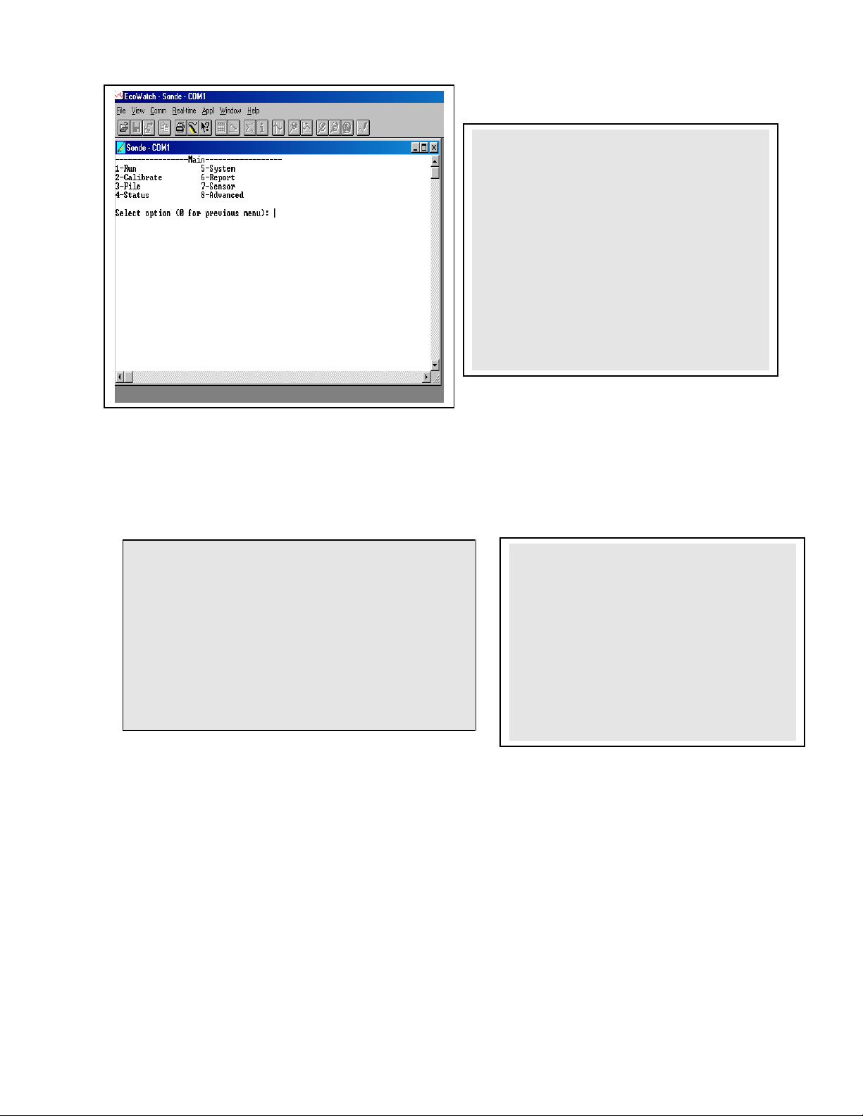
Sondes Section 2

Filename Samples

1-BRIDGE1.dat 19 2-BRIDGE2.dat 27 3-UPLAKE.dat 33 4-CLRLAKE2.dat 167 5-DWNLAKE2.dat 31 6-00003001.glp 3

Select option (0 for previous menu): 4

-----------------File-----------------

1-Directory 4-View file 2-Upload 5-Quick view file 3-Quick Upload 6-Delete all files

Select option (0 for previous menu): 1

-------------File details--------

-----1-View file 2-File:CLRLAKE2.dat 3-Samples: 167 4-Bytes: 4421 5-First:08/23/2001 6-First:08:33:40 7-Last :08/23/2001 8-Last :09:04:20 9-Interval:00:00:10 A-Site:Clear Lake

Select 1-Directory to view all files currently stored in the sondes flash disk memory, the screen below shows 6 files. All data files (.dat extension) could be uploaded to EcoWatch for viewing or plotting, but you do not need to upload all files in the directory. The file with the .glp extension contains the calibration record of the sonde. It is fully described in Sections 2.9.2 and 2.9.3 below. Details of any of the studies can be obtained by pressing the number key associated with the file in the Directory.

Select 2-Upload to view file lists in memory, and upload the data to PC-based software.

Prior to upload, a “Time window” display appears that will allow you to select portions of the logged data to upload. You may select 1-Proceed to upload all logged data from the dates and times displayed.

YSI Incorporated Environmental Monitoring Systems Operations Manual 2-55

Sondes Section 2

--------------Time window-------------1-Proceed 2-Start date=08/14/96 3-Start time=18:00:00 4-Stop date=08/28/96 5-Stop time=11:00:00

Select option (0 for previous menu):

---------------File type--------------1-PC6000 2-Comma & ' ' Delimited 3-ASCII Text

Select option (0 for previous menu):

Select 1-Proceed. Choose the appropriate file transfer protocol (in this example, PC6000) and a status box will show the progress of the upload. Verification of a successful transfer is indicated when all of the requested data have been transferred to the C:\ECOWIN\DATA subdirectory of your PC and automatically assigned a “.DAT” extension.

Select 3-Quick Upload to transfer the last logged file in its entirety to your computer. As noted above, the file will then be resident in the C:\ECOWIN\DATA subdirectory.

Select 4-View File to examine the data in any file currently stored in the sondes flash disk memory. You will first view the same screen as viewed in the Directory menu. From this menu choose the file of interest, then, using the Time window menu, choose the dates and/or times of interest. If you choose dates or times that are not within the designated start and stop times, no data will be displayed.

You also may choose the entire file. You can use the Space Bar to stop and restart the scrolling at any time. Use the Esc key to stop the view.

YSI Incorporated Environmental Monitoring Systems Operations Manual 2-56

Sondes Section 2

Select 5-Quick view file to view the last page of data from the last data file in flash disk memory. This feature is particularly useful to quickly review any recently acquired data so that system performance can be assessed.

Select 6-Delete all files to IRREVERSIBLY remove all files (INCLUDING the .glp file that contains

calibration information) from the sonde flash disk memory. It is critical not to use this option until all relevant data from sonde memory is transferred to your computer via one of the upload options. There is a verification screen that appears, so that pressing the number 6-key does not immediately delete all files.

NOTE: By choosing the Delete function only .dat and .glp files will be erased. Calibration data for all sensors installed and calibrated on the sonde will not be deleted.

REPORTING AND PLOTTING DATA WITH ECOWATCH

There are many features in EcoWatch related to viewing, plotting, manipulating and reporting data collected from a 6-Series sonde. EcoWatch includes a Windows Help section for convenient reference that describes all of the software‟s features. This section of the manual describes the most commonly used functions of the program and Section 4, EcoWatch for Windows, is a detailed manual for EcoWatch software.

For the purposes of describing and demonstrating EcoWatch plotting, reporting and data manipulation capabilities, we use the file SAMPLE.DAT available on the compact disk that was enclosed with your 6series sonde. This file will be copied to your hard drive during EcoWatch installation and should be available to you for the instructions below.

When you are ready to move beyond the example SAMPLE.DAT file and analyze data collected from the sonde, locate and open the appropriate .DAT file from your data upload exercise. These data are normally found at C:\ECOWWIN\DATA\. An example filename is 1097CM01.DAT.

NOTE: In the instructions below that refer to clicking the mouse button, we always refer to the left mouse button unless otherwise specified.

OPENING A DATA FILE

If EcoWatch is not running, open the program by double clicking on the EcoWatch icon. Click on File to view a drop-down menu similar to the one shown in Figure 41. From this menu click on Open, then locate the drive and directory where SAMPLE.DAT (or your file of interest) resides. Alternatively, if you have been using EcoWatch during setup and checkout, you may be able to click on the file of your choice in the most recently opened files.

Once the SAMPLE.DAT file is open you should see a plot, Figure 41, which graphically represents seven days of sonde data for six different water quality parameters plotted as a function of date and time. Each set of data is autoscaled to allow you to see the minimum and maximum values for each parameter during the one-week study.

YSI Incorporated Environmental Monitoring Systems Operations Manual 2-57

Sondes Section 2

Figure 41 Opening a File

Some daily variations may be noticed in parameters such as dissolved oxygen, pH and temperature in this particular study. This is fairly typical in many natural bodies of water. Note also that conductivity is low at both ends of the graph. You may notice similar perturbations in some of the other readings as well. In this example, the sonde was not in the water for a short time at the beginning and end of the study. Not only can you see exactly when the sonde went in and out of the water, but the bottom graph shows the depth at which the sonde was deployed.

Notice also that you now see a new set of menu items in the top line. Some of these functions are specifically related to viewing and manipulating data. Next we will examine some of the viewing options.

VIEWING DATA

To look at some of the viewing options, click on View (Figure 42). Note that the Toolbar and Status Bar are turned on (check mark). In addition, the 4-Digit Year expression is checked. Also note that a check mark is just left of the Graph choice. When a check is next to Graph, all data are expressed graphically in the opening window.

To show data in both graphical and data table format, highlight the Table menu item, then click or press Enter. The graphical portion of the window becomes compressed, and the data table becomes visible. If you then click on View again, both the Graph and Table items have check marks to their left, indicating that both functions are turned on. You may use your mouse to scroll up/down and left/right to view data.

YSI Incorporated Environmental Monitoring Systems Operations Manual 2-58

Sondes Section 2

Figure 42 Viewing Options

It may be somewhat awkward to scan the data table in this manner; therefore you have the option to turn off the graphical representation and allow the table to fill the window. See Figure 43. Notice now that when you click on View, the Graph item is no longer checked.

YSI Incorporated Environmental Monitoring Systems Operations Manual 2-59

Sondes Section 2

Figure 43 Viewing the Data in Table Format

Viewing features such as Grid, Marker, Zoom In, Zoom Out and Unzoom are all available when you activate the Graph function. Give each a try as you practice and learn more about the many features of EcoWatch.

The Statistics and Study functions of EcoWatch are shown in Figure 44. Both provide overview information related to the study data. The Statistics function lists minimum, maximum, mean and standard deviation information for each parameter activated. The Study function provides useful information about the design of the study including sample interval, date/time, number of samples, sensor identification and parameters reported. The Statistics and Study windows may be activated over either graph or table presentations.

To view either of these windows, click on View, highlight the desired function and click again. The window opens on top of the table or graph, similar to what is shown in Figure 43. Only one of these windows may open at one time. To continue, you must close the Statistics or Study window to return to the graph or table and activate the top line menu again.

As before practice viewing the functions mentioned above to gain more familiarity with these features.

YSI Incorporated Environmental Monitoring Systems Operations Manual 2-60

Sondes Section 2

Figure 44 Statistics and Study Information

Next, with the Statistics and Study windows closed, return to the View menu, close Table and activate Graph.

Using the right mouse button, click at any point on the graph. A dotted vertical line appears along with specific data values in boxes to the left of the displayed graphs, as shown in Figure 45. You can hold down the right mouse button and move the mouse to scan the entire graph that is displayed in the window. The values in the boxes change as you move the mouse. This feature is very useful for quantifying specific data without the need to open the data table and scroll through what may be thousands of data points. Note also that the exact time and date change to let you know specifically when an event of interest occurred.

YSI Incorporated Environmental Monitoring Systems Operations Manual 2-61

Sondes Section 2

Figure 45 Viewing the Data with Right-Button Mouse Function

CHANGING DISPLAY FORMATS USING SETUP

Beyond selecting data viewing options such as table format or graphical format, you may also customize your data displays. For example, you may change the order in which parameters are viewed, you may add and delete parameters, you may change plot appearance using different interval times and different units, and you may change the x-axis if you prefer a parameter other than date or time.

The Top Line menu selection that allows you to select some of these parameter changes is Setup. Click on Setup, then Parameters. From here there are four submenus that allow you to Add/Remove parameters, change Units, change sample interval and/or x-axis (Attributes) and change the Names of the parameters you have assigned, as shown in Figure 46.

YSI Incorporated Environmental Monitoring Systems Operations Manual 2-62

Sondes Section 2

Figure 46 Changing the Appearance of a Graph or Table

If you are displaying the graph, you may change the appearance by changing font, font style, size and text color. You may also change page color, trace color and graph background color. You may assign a custom 2-line title for the graph, and finally, you may display 1 trace or 2 per set of axes. For display of table formatted results you may change font, font style, size and text color. In addition, you may change table color and highlight color.

The menu structure is easy to follow. Try some changes to gain familiarity with these Setup display options.

CHANGING DISPLAY FORMATS USING „GRAPH‟ FUNCTION

The top line menu labeled Graph, as the name suggests, can be used to examine critical events within the graphical format. You may be able to more clearly understand an event by zooming in/out, centering an event of interest, and setting limits to focus in on a specific area of the graph. In addition to modifying

YSI Incorporated Environmental Monitoring Systems Operations Manual 2-63

Sondes Section 2

along the x-axis, you may also manually scale the y-axis. This may allow you to discard a noise spike and obtain better resolution of events unrelated to the noise. Functions like Autoscale, Redraw and Cancel Limits are all used to “undo” some of the customization functions. Below in Figure 47 you see some of these functions.

One very commonly used function is Limit Data Set. If you choose this function by clicking on the highlighted item as shown below, you then use the mouse to move your cursor to the left limit of an area of interest, click once, then move the mouse to the right limit of interest and click again. The result will be a close up look at the specific area of the graph you have defined. Refer to Figure 47 and 48 below to see the results of this particular feature.

Figure 47 Selecting a Subset of Data within a Graph

YSI Incorporated Environmental Monitoring Systems Operations Manual 2-64

Sondes Section 2

Figure 48 Using Limit Data Set to Display a Subset of Data

To return to the full set of data again, click on Graph, then Cancel Limits. If you desire a hard copy of any graph or table, or even a subset expression as shown above, you may use the Edit, Copy command to „copy‟ the graph in the active window to the “Clipboard”. You can then „paste‟ this graph to the Windows application program of your choice. You may also be able to print graphs and tables as described in the next section.

SAVE, IMPORT, EXPORT AND PRINT COMMANDS

Under File function in the top line menu, you can save a particular presentation version of a data file and give the presentation a customized name. For example, you might want to call the expanded plot in Figure 48 “DIURNAL” using the File|Save Data Display command. This presentation will be saved with your data file and can be recalled in further by using the File|Load Data Display command. You can also export your custom data display as a spreadsheet compatible file (.CDF or .TXT) or print it to a compatible printer. You may also create a custom report format using the File|Report command. See Figure 49 for the File menu, which shows these commands. Use the Window‟s Help function to learn more about these features.

YSI Incorporated Environmental Monitoring Systems Operations Manual 2-65

Sondes Section 2

Figure 49 Saving, Exporting, Printing and Related Functions

EXAMPLE OF CUSTOMIZING A SUBSET OF SAMPLE.DAT

To conclude this section we have used a few of the many tools available in EcoWatch to demonstrate how you might use this powerful plotting and reporting program to express study results. We encourage you to try some of the tools and learn more about EcoWatch by using the Window‟s Help function, which is available when the EcoWatch program is running.

Using SAMPLE.DAT we decided that some of the data were not of particular interest, so using top line menu item Setup, then Parameters, then Add/Remove, we removed ORP and Depth results from the data set. Note that we have not deleted this information from the file, but rather we are choosing not to display it. You can always return to this function and add original data back. Under the same Parameters function, we have selected Attributes and changed the Average Interval from the default 0 to 60. Since data was collected every 15 minutes, the change to a 60 minute interval helps to smooth out the graph and average out any short term “noise” events.

Next, we again select Setup, then Graph. From the functions available, we first selected Title Page… and typed in a name (Clear Lake Study #2) and below that we typed the parameters that are shown in the graph. Just below Title Page, we clicked on 2 Traces per Graph. This combines adjacent parameters which is sometimes useful in parameter and event evaluation. For example, in the second graph shown in Figure 50 below, you see that DO concentration and pH seem to track rather closely and change in a diurnal rhythm. In actuality, when DO levels drop in a natural body of water, CO2 often builds up forming carbonic acid which leads to lower pH readings. DO rises again during the day due to photosynthesis, CO2 then falls and pH increases again. The final plot after making these changes in shown in Figure 50.

YSI Incorporated Environmental Monitoring Systems Operations Manual 2-66

Sondes Section 2

Figure 50 Customizing a Graph from SAMPLE.DAT

Finally, we selected File|Save Data Display and gave the custom plot the name “4PARAM” to that the presentation can be immediately recalled in the future.

As you become more familiar with EcoWatch for Windows, the plotting, analysis and reporting functions can be accomplished easily and quickly. Practice with all of the functions and, again, do not forget to use Window‟s Help for more detail, or see Section 4, EcoWatch for Windows.

YSI Incorporated Environmental Monitoring Systems Operations Manual 2-67

Sondes Section 2

IMPORTANT MESSAGE!

WHAT IF THERE IS NO RESPONSE TO A KEYSTROKE?

To save power, the sondes will power down automatically if no interaction from the keyboard occurs for approximately 60 seconds. When the software is in this “sleep” mode, the first subsequent keystroke simply “wakes it up” and has no visible effect on the display. The next keystroke after the unit is “awakened” will be input to the software in the intended manner. Thus, if you press a key after the sonde has been inactive for some time and nothing seems to happen, press the key again.

2.9 SONDE MENU

The functions of the sondes are accessible through the sonde menu. The sonde menu structure makes it simple and convenient to select functions. This section provides a description of the menus and their capabilities.

When moving between menus within the sonde software structure, use the 0 or Esc to back up to the previous menu. To exit menus and return to the sonde command line (the # sign), press 0 or Esc until the question “Exit menu (Y/N)?” appears. Type Y and the command prompt (“#”) will be shown. To return to the Main sonde menu, type menu and press Enter.

To gain experience with the sonde menus, select the sonde icon in EcoWatch for Windows and press Enter. See Figure 40 above for the Sonde Menu Flow Chart.

In the following subsections you will learn about the functions of the various menu items and when to use them. The discussion of the menu and submenu functions is organized in numerical order, beginning with

Section 2.9.1 Run

YSI Incorporated Environmental Monitoring Systems Operations Manual 2-68

Sondes Section 2

---------------Run setup--------------1-Discrete sample 2-Unattended sample

Select option (0 for previous menu): 1

------------Discrete sample-----------1-Start sampling 2-Sample interval=4 3-File= 4-Site= 5-Open file

Select option (0 for previous menu):

2.9.1 RUN

Select 1-Run from the Main menu to begin taking readings or to set/verify the parameters required for a study. There are two options in the Run menu.

DISCRETE SAMPLING

Discrete sampling is usually used in short term, spot sampling applications when the user is present at the site and the unit is attached to a 650 MDS Display/Logger or laptop PC. It could be used in the vertical profiling of a lake or river where the user lowers the sonde incrementally into the water, and data acquired for a few minutes at each depth. In this section, you will learn how to use the sonde menu structure to open and close files, set the interval between samples, start the sampling operation, and log data to the internal memory of the sonde.

Select 1-Discrete sample from the Run menu. The Discrete sample menu will be displayed.

YSI Incorporated Environmental Monitoring Systems Operations Manual 2-69

Sondes Section 2

============================================================================= Date Time Temp SpCond Sal DO Depth pH Turbid Battery

mm/dd/yy hh:mm:ss C mS/cm ppt mg/L feet NTU volts

-----------------------------------------------------------------------------*** 1-LOG last sample 2-LOG ON/OFF, 3-Clean optics*** 05/05/97 10:04:40 21.57 0.009 0.00 7.73 -0.293 7.55 0.3 10.2 05/05/97 10:04:44 21.57 0.009 0.00 8.41 -0.300 7.55 0.3 10.3 *** LOG is ON, hit 2 to turn it OFF, 3-Clean optics*** 05/05/97 10:04:48 21.58 0.009 0.00 8.41 -0.302 7.55 0.3 10.3 05/05/97 10:04:52 21.58 0.009 0.00 8.40 -0.302 7.55 0.3 10.3 05/05/97 10:04:56 21.58 0.009 0.00 8.41 -0.303 7.55 0.3 10.2 05/05/97 10:05:00 21.58 0.009 0.00 8.42 -0.303 7.55 0.3 10.3 *** 1-LOG last sample 2-LOG ON/OFF , 3-Clean optics*** 05/05/97 10:05:04 21.58 0.009 0.00 8.44 -0.304 7.55 0.3 10.3 Sample logged. 05/05/97 10:05:08 21.58 0.009 0.00 8.45 -0.305 7.55 0.3 10.3

Select 1 – Start sampling option to start discrete sampling. After the initial sampling time interval has passed (4 seconds in the screen above), sequential lines of data will appear on the screen.

The following prompt will appear just below the screen header:

1-LOG last sample, 2-LOG ON/OFF, 3-Clean optics

 By entering 1–LOG last sample, A single line of data can be logged to sonde memory and the

following message will be displayed: Sample logged.

 By entering 2-LOG ON/OFF, a set of data can be logged to memory and the following message will

be displayed: LOG is ON, hit 2 to turn it OFF, 3-Clean optics. Press 2 again to terminate logging.

 By entering 3-Clean optics, if your unit has an optical probe, the wiper will clean the optical surface.

The 3-Clean optics portion of the prompt will only appear if an optical probe was installed and enabled.

Select Esc or press 0 and return to the Discrete Sampling menu.

From the Discrete Sampling menu, select 2-Sample Interval to type a number that represents the number of seconds between samples. The maximum sample interval is 32767 seconds (9+ hours). The factory default sample interval is 4 seconds and works best for most discrete sampling applications. The shortest possible sample interval for obtaining new DO readings is 4 seconds. If a smaller interval is selected, then the DO readings remain constant for the number of samples necessary to fill 4 seconds.

NOTE: If your have used your sonde with a 650 MDS data logger, the Sample Interval automatically be changed to 0.5 seconds.

YSI Incorporated Environmental Monitoring Systems Operations Manual 2-70

Sondes Section 2

Sampling Faster Than 0.5 Seconds

For special applications, your sonde is capable of faster sampling. The only limitation is a reduction of the number of sensors selected. To determine the maximum sampling frequency for your sensor setup, divide 36 by the number of enabled sensors in addition to the DO sensor.

Example:

If you enable any three sensors plus DO, divide 36 by 3 to obtain 12 samples/second (12 Hz) or 0.083 seconds between samples as the maximum sampling frequency. Remember that for sample intervals less than 4 seconds, DO readings are updated only every 4 seconds. Thus, at 12 Hz, the display will show 48 identical DO readings before a change occurs. Note also that at a faster sampling rate, consecutive readings are closer together, the threshold for any one sensor is less likely to be exceeded, and the data filter is less likely to disengage. For these applications you may want to adjust your threshold settings accordingly. See Section 2.9.8 for more information on the data filter.

Select 3-File to enter a filename with a maximum of 8 characters. You will log readings to the filename that you enter.

Select 4-Site to assign a site name with a maximum of 31 characters This allows you to enter the name of the site where you are sampling.

When you select 5-Open File, a file is opened and the number 5 changes to Close File. When you are finished logging data to the file, press 5-Close File and designation changes back to Open File. When you start logging the Open File designation changes automatically to Close File.

Now select 1-Start sampling to start discrete sampling.

After the initial sampling time interval has passed, sequential lines of data will appear on the screen and you can log single or sequential data points and wipe the surface of your optical probe as described above.

UNATTENDED SAMPLING

This option is used for long-term deployment of the battery-powered sonde when the user is not present at the site. Prior to this selection, the sonde is usually attached to a computer in a laboratory and set up to automatically log data to sonde memory at a fairly long time interval (15-60 minutes). The unit is then taken to the field site and left for an extended time period (from 30 up to 150 days depending on the sensors used and the fouling conditions). When the study is complete, or the batteries are expended, the unit is brought back to the laboratory and the data file is uploaded to a computer. Quality assurance checks are performed prior to redeployment.

Select 2-Unattended Sampling from the Run menu. The Unattended sample menu will be displayed. Use the following example to understand the unattended sampling option.

YSI Incorporated Environmental Monitoring Systems Operations Manual 2-71

Sondes Section 2

------------Unattended setup----------1-Interval=00:15:00 2-Start date=07/17/96 3-Start time=18:00:00 4-Duration days=14 5-File=clrlake3 6-Site=Clear Lake at Spillway 7-Bat volts: 9.1 8-Bat life 21.2 days 9-Free mem 18.9 days A-1st sample in 8.10 minutes B-View params to log C-Start logging

Follow the prompts on this screen to prepare your sonde for unattended deployment as described below:

 Verify that the current time and date are correct to ensure that your unattended sampling study begins

and ends when you desire. To verify correct the time and date, return to the Main menu and enter 4- Status or 5-System. You may enter the correct date and time from either of these submenus.

 Select 1-Interval and enter the desired time between samples

 Select 2-Start Date and 3-Start Time to set the time that data will begin to log to sonde memory. .

Use the 24-hour clock format to enter the time. If you do not make any change to these entries, then the study will automatically begin at the next integral time interval once you have pressed C-Start

logging.

Example: If the current time is 17:20:00 and your sample interval is 15 minutes, logging will

automatically begin at 17:30:00.

It is better to start the study prior to taking the unit to the field so that you can confirm that readings are being saved to memory and carry out initial quality assurance. However, if your study demands that you start the instrument at the site at 6:00 PM, change the Start Time to 18:00:00.

 Select 4-Duration and set the length of the study in days. The default value is 365 days (which is

 Select 5-File and enter a name of no more than 8 characters that will be used by your external

computer to identify the study. Be sure to use ONLY alpha/numeric characters.

 Select 6-Site and enter a site name of no more than 31 characters. This filename will appear in your

sonde file directory, but will not be used to identify the file after transfer to your computer.

 Check 7-Battery to make certain that the voltage is suitable for the length of the study that you are

about to begin. No change can be made to this item via the software. Note that no battery entry will appear for the 600R, 600QS, 600XL, and 6820V2-1 sondes.

YSI Incorporated Environmental Monitoring Systems Operations Manual 2-72

Sondes Section 2

-------------Params to log------------1-Temp C 6-Orp mV 2-Cond mS/cm 7-NH4+ N mg/L 3-DOsat % 8-NO3- N mg/L 4-DOchrg 9-Turbid NTU 5-pH A-Battery volts

Select option (0 for previous menu):

-------------Start logging------------Are you sure? 1-Yes 2-No

Select option (0 for previous menu):

 Select B-View Parameters to log to confirm that your sensor and report setups are configured

correctly as described in Sections 2.9.6 and 2.9.7. An example screen is shown below.

In some cases, the View params to log screen only identifies the raw parameters that are used in the calculation of the items that you have selected in the Report setup.

Example: You have selected DO mg/L in the Report setup, but it does not appear under View parameters to log because it is calculated from DO saturation %,Temperature, and Conductivity.

Likewise, although specific conductance is selected in the Report setup, it does not appear under Parameters to log because it is calculated from Conductivity and Temperature. In all but a few cases, the proper configuration of Parameters to log will be automatically set up as long as the sensor is enabled.

There are several items that must be activated in the Report setup so they will be available from the file after upload. These special parameters are: DO Chg, DOSat %Local, ODOsat %Local, pH mV, NH4+ mV, NO3- mV, Cl-mV, PAR1, PAR2, Chl RFU, BGA-PC RFU, and BGA-PE RFU. If you want to log any of these parameters to your data file, be certain that they are active in the Report setup before you begin the unattended study.

After making the above entries, the sonde software will automatically estimate the expected battery life, and the time it will take for the sonde memory to be filled. This information is displayed on the screen for your consideration. If the battery life or the free memory capacity will be exceeded sooner than the duration, you may want to make some changes to the sonde set-up or the batteries themselves. For example, you can free up memory in the sonde by uploading all existing files from the sonde memory to your PC and then deleting them from the sonde (see 3-File from Main Menu). You may want to change the batteries for longer battery life. You can lengthen the sampling interval to extend both battery life and memory capacity.

The predicted battery life is an estimate only. The temperature of the site and the brand of batteries used can affect battery life. It is recommended to recover the sonde earlier than the predicted battery life, and to use new batteries for each deployment.

Once you press C-Start logging, the following screen will appear.

YSI Incorporated Environmental Monitoring Systems Operations Manual 2-73

Sondes Section 2

----------------Logging---------------1-Interval=00:15:00 2-Next at 07/17/96 3-Next at 18:00:00 4-Stop at 07/31/96 5-Stop at 18:00:00 6-File=clrlake3 7-Site=Clear Lake at Spillway 8-Bat volts: 9.0 9-Bat life 21.2 days A-Free mem 18.9 days B-Stop logging C-Show Live Data

Select option (0 for previous menu):

Stop logging? 1-Yes 2-No

Select option (0 for previous menu):

Select 1-Yes and the screen will change.

The display now shows the next date and time for logging and the stop date and time for the logging study. Most importantly, note that the bottom command now shows B-Stop logging, a confirmation that the logging has indeed been initiated.

If you select C-Show Live Data and leave the sonde attached to your PC, the data points will be shown on the screen as they are stored to internal memory.

YSI Incorporated Environmental Monitoring Systems Operations Manual 2-74

Sondes Section 2

2.9.2 CALIBRATE

All of the sonde sensors (except temperature) require periodic calibration to assure high performance. However, the calibration protocols for Rapid Pulse Polarographic dissolved oxygen are significantly different depending on whether the sonde is being set up for spot sampling or longer term unattended monitoring studies. This difference is user-selectable and is required primarily because the optimal performance of the Rapid Pulse dissolved oxygen sensor cannot be attained unless the control of this sensor varies from short term to long term applications.

For spot sampling it is best to pulse the sensor continuously during the Run mode to attain the most accurate results and optimize the response time. However, this continuous pulsing is not ideal for longer term logging studies in which the sonde data is captured to sonde memory or to a data collection platform at much less frequent intervals (e.g. 15 minutes). Continuous pulsing not only shortens the time between required probe maintenance, but consumes more power. With proper selection of the “Auto sleep” option (discussed in detail in Section 2.9.8, Advanced Menu), the user can configure the sonde software to either run continuously or “go to sleep” between samples to minimize Rapid Pulse DO probe wear and conserve power. The effect of this choice on the user interface relative to dissolved oxygen calibration is significant as described below:

 If “Auto sleep” is deactivated, the sonde runs continuously no matter what sample interval has been

selected. Under these conditions, the user retains manual control of the dissolved oxygen calibration routine, viewing the stabilization of the readings in real time and confirming the calibration with keyboard entries.

 If “Auto sleep” is activated, the sonde will „warm up‟ the sensors for the period of time selected for

the DO sensor. Under these conditions, the user loses manual control of the Rapid Pulse DO calibration routine. Rapid Pulse DO will automatically calibrate after the selected time for warm up of the DO sensor has expired. In this mode of calibration, you do not observe stabilization of the readings in real time, but instead will observe a countdown of the warm up period followed by a message indicating that the Rapid Pulse DO calibration is complete.

Only the calibration of Rapid Pulse dissolved oxygen is affected by whether “Autosleep” is on or off; the user retains manual control of the calibration of all other parameters regardless of the “Auto sleep” setting. Once a particular warm up time (in seconds) has been utilized in Rapid Pulse DO calibration, the length of that time should not be changed during a study. A new calibration should be performed whenever the value of the warm up time is altered.

Note that the ROX Optical DO sensor is not subject to the above issues relative to the activation of “Autosleep RS232” for the Rapid Pulse DO sensor. The ROX sensor calibrates in the same way as any other sensor such as conductivity, pH, or turbidity where the user manually confirms the calibration after the sensor readings have shown stability.

From the Main sonde menu select 2-Calibrate. The Calibrate menu will be displayed. Only the enabled parameters will be available for calibration.

YSI Incorporated Environmental Monitoring Systems Operations Manual 2-75

Sondes Section 2

---------------Calibrate-------------1-Conductivity 6-ISE3 NH4+ 2-Dissolved Oxy 7-ISE4 NO33-Pressure-Abs 8-ISE5 Cl4-ISE1 pH 9-Optic T-Turbidity 6136 5-ISE2 ORP A-Optic C - Chlorophyll

Select option (0 for previous menu):

CONDUCTIVITY

Select 1-Conductivity to calibrate the conductivity probe and a second menu will offer you the options of calibrating in specific conductance, conductivity, or salinity. Calibrating any one option automatically calibrates the other two. After selecting the option of choice (specific conductance is normally recommended), you will be asked to enter the value of the standard used during calibration. Be certain that the units are correct. After pressing Enter, you will be able to follow the stabilization of the readings and confirm the calibration when the readings are stable by pressing Enter as instructed on the screen. Then, as instructed, press Enter again to return to the Calibrate menu.

RAPID PULSE POLAROGRAPHIC DISSOLVED OXYGEN WITH AUTOSLEEP ON

If you intend to do Unattended Sampling, it is recommended that you turn Autosleep RS232 “on” in the Advanced|Setup menu and follow these instructions for DO calibration. If you intend to do Discrete Sampling, it is recommended that you turn Autosleep RS232 “off” and use the calibration instructions in the next section.

Select 2-Dissolved oxygen to calibrate the oxygen probe. The submenu will offer you the option of calibrating in percent saturation or mg/L. After selecting the option of choice (percent saturation in watersaturated air is normally recommended), you will be prompted for the next step. Calibrating either of the choices will automatically calibrate the other.

For the percent saturation mode, be certain that the sensor has been thermally equilibrated in watersaturated air and that the sensor shows stable readings prior to beginning the calibration routine, particularly after a membrane change. Note, however, that the sensor should be “off” for at least 5 minutes before initiating a calibration procedure with “Autosleep” active. If possible, it is ideal that the sensor be “off” for a time equal to the sample interval in the upcoming study.

Remember, the Calibration Cup is designed to be air-tight and must be loosened if it is used as a calibration chamber. See Section 2.6, Calibration for more details. Follow the screen prompt and enter

the local barometric pressure in mm Hg, (inches Hg x 25.4), press Enter, and the calibration will automatically occur after the warm-up time which has been selected by the user (default is 40 seconds). Then, as instructed, press Enter again to return to the Calibrate menu. Note that at calibration, the DOsat % (percent air saturation) value will reflect the barometer value that was entered. For example, if a barometric pressure of 720 mm is entered, the DOsat % value will change to 94.7 % (720/760 x 100).

Note that the parameter “DOsat %Local” is also available for users who prefer to set their percent air saturation value to 100%, no matter what barometer value is entered. The method of activating this parameter, its use, and its limitations are described in Appendix J of this manual. The key factor to remember, however, is that no matter which convention (DOsat % or DOsat %Local) is selected, the mg/L value will not be affected.

YSI Incorporated Environmental Monitoring Systems Operations Manual 2-76

Sondes Section 2

For the mg/L mode, calibration is carried out in a water sample which has a known concentration of dissolved oxygen, usually determined by Winkler titration. For this calibration procedure, the sensor should be immersed in the water. After thermal equilibration, enter the known mg/L value, press Enter, and the calibration procedure will be carried out automatically as for the percent saturation mode above.

RAPID PULSE DISSOLVED OXYGEN WITH AUTOSLEEP OFF

If you intend to do Discrete Sampling, it is recommended that you turn Autosleep “off” in the Advanced|Setup menu and follow these instructions for DO calibration. If you intend to do Unattended Sampling, it is recommended that you turn Autosleep “on” and using the calibration instructions in the preceding section.

Select the Dissolved Oxygen option from the Calibrate menu to calibrate the oxygen probe. The submenu will offer you the option of calibrating in percent saturation or mg/L. After selecting the option of choice (percent saturation in water-saturated air is normally recommended), you will be prompted for the next step. Calibrating either of the choices will automatically calibrate the other.

For the percent saturation mode, be certain that the sensor has been thermally equilibrated in watersaturated air and that the sensor has stabilized prior to beginning the calibration routine, particularly after a membrane change. Relieve pressure in the cup if necessary. Remember, the Calibration Cup is designed to be air-tight and must be loosened if used as a calibration chamber. Then follow the screen prompt and enter the local barometric pressure in mm Hg, (inches Hg x 25.4), press Enter, and monitor the stabilization of the DO readings. After no changes occur for approximately 30 seconds, press Enter to confirm the calibration. Then, as instructed, press Enter again to return to the Calibrate menu. Note that at calibration, the DOsat % (percent air saturation) value will reflect the barometer value that was entered. For example, if a barometric pressure of 720 mm is entered, the DOsat % value will change to 94.7 % (720/760 x 100).

For the mg/L mode, calibration is carried out in a water sample which has a known concentration of dissolved oxygen, usually determined by a Winkler titration. For this calibration procedure, the sensor should be immersed in the water. After thermal equilibration, enter the known mg/L value, press Enter, and the calibration procedure will begin with similar viewing of stabilization and confirmation of calibration as for the percent saturation mode above.

NOTE: If you have resurfaced your DO sensor, we recommend running the probe continuously for 15-30 minutes or until good stability is realized. After only a membrane change (no resurfacing), run the probe continuously for 3-4 minutes or until good stability is realized.

ROX OPTICAL DISSOLVED OXYGEN

Understanding the Factory Calibration of the ROX Optical DO Sensor

Unlike all other sensors for YSI 6-series sondes, the response of the ROX Optical DO sensor is not linear relative to the species being measured. This non-linearity requires that the sensor be factory-calibrated at a number of oxygen values and the data fit to a third-order regression. The three constants and the sensor value at zero dissolved oxygen which define this regression analysis are automatically stored in the sensor at the time of factory-calibration. It is important to note that these constants are a function of the sensor

YSI Incorporated Environmental Monitoring Systems Operations Manual 2-77

Sondes Section 2

membrane installed on the 6150 probe and NOT a function of the probe, i.e., the constants reflect the characteristics of the sensor membrane and NOT the probe. When a 6150 probe is purchased from YSI, it already has a sensor membrane installed and the constants of that membrane are transferred automatically to the sonde PCB when the sensor is run for the first time. After transfer, the constants can be viewed by accessing the Advanced|Cal Constants menu as shown below – the regression constants are ODO K2ODO K4 and the value at zero oxygen is K1 as shown below.

It should also be noted that the ROX sensor is characterized by two additional parameters – ODO Gain and Tzero. The ODO gain reflects the small change in the calibration which is carried out be the user in a 1point calibration as described below. The Tzero value will always be the same as K1 until the user elects to perform a 2-point calibration as described below at which time it will change slightly to reflect the adjustment of the zero oxygen value.

You will also note that a different set of constants for your specific sensor membrane are supplied on the instruction sheet which came with your 6150 probe. These five constants (K1-K4 and C) have a different appearance than those shown in Advanced|Cal Constants because they are in coded form to allow errorfree reentry by the user in the unlikely event that the regression constants in the probe are lost. The C constant is a check sum value associated with the values of K1-K4 and will prevent acceptance of the constants if typographical errors are made in their entry by the user. The coded constants must be entered in the Calibrate|Optic X – Dissolved Oxy|Enter Cal Sheet as shown below. The constants can also be viewed at any time by selecting Calibrate|Optic X – Dissolved Oxy|View Cal Sheet.

YSI recommends that your replace your sensor membrane after 1 year of use by purchasing the 6155 Optical DO Membrane Replacement Kit. This kit will be supplied with a new set of coded constants

YSI Incorporated Environmental Monitoring Systems Operations Manual 2-78

Sondes Section 2

which characterize the new membrane and they MUST be entered via the Calibrate|Optic X – Dissolved Oxy|Enter Cal Sheet selection as show above. Once the new constants have been entered in coded form

they will be transferred to the probe and will be visible in uncoded form in Advanced|Cal Constants.

See Section 5.9, Principles of Operation and Appendix M, ROX Optical DO Sensor for more information.

User Calibration of the ROX Optical DO Sensor

NOTE CAREFULLY: As opposed to the 6562 Rapid Pulse Polarographic DO sensor described above,

there is no difference between the calibration routine for sensors which will be used for sampling or monitoring applications. Usually the Autosleep RS-232 feature in the Advanced|Setup menu will be activated for ROX calibrations, but there is no problem if it is not active.

Select the Optic X-Dissolved Oxy option from the Calibrate menu to calibrate the oxygen probe. The submenu will offer you the option of calibrating in either percent air-saturation (ODOsat %) or oxygen concentration (ODO mg/L) units. Calibrating either of the choices will automatically calibrate the other. After selecting the option of choice (ODOsat % in water-saturated air or air-saturated water is normally recommended), you will be prompted for the next step where you must elect to do either a 1-point or a 2point calibration. Except under unusual circumstances as described below, you should select the 1-point option for the ROX Optical DO calibration.

Calibration Using Percent Air Saturation – 1-Point

NOTE: YSI recommends that you use this method for calibration of your 6150 Dissolved Oxygen Sensor to obtain the maximum accuracy under normal operating conditions.

Enter the current barometric pressure in mm of Hg. (Inches of Hg x 25.4 = mm Hg).

Note: Laboratory barometer readings are usually “true” (uncorrected) values of air pressure and can be used

True BP = [Corrected BP] – [2.5 * (Local Altitude in feet above sea level/100)]

The minor advantages and disadvantages of calibration in air-saturated water versus water-saturated air are outlined in Appendix M, ROX Optical DO Sensor

YSI Incorporated Environmental Monitoring Systems Operations Manual 2-79

Sondes Section 2

Calibration Using mg/L – 1-Point

Place the sensor in a container which contains oxygen of a known concentration of dissolved oxygen in mg/L AND THAT IS WITHIN +/- 10% of AIR SATURATION as determined by one of the following methods:

 Winkler titration  Aerating the solution and assuming that it is saturated, or  Measurement with another instrument.

CAUTION: Carrying out DO mg/L calibrations at values outside the range of +/- 10 % of air saturation is likely to compromise the quoted accuracy specification of the 6150 Optical DO Sensor.

Wait approximately 10 minutes before proceeding to allow the equilibration of the temperature and oxygen sensors.

Select ODO mg/L and then 1-Point to access the mg/L calibration procedure. Calibration of your optical dissolved oxygen sensor using the DO mg/L procedure also results in calibration of the ODOsat % mode and vice versa.

Enter the known mg/L concentration and press Enter. The current values of all enabled sensors will appear on the screen and change with time as they stabilize. Observe the readings under ODO mg/L and, when they show no significant change for approximately 30 seconds, press Enter. The screen will indicate that the calibration has been accepted and prompt you to press Enter again to return to the Calibrate menu.

2-Point Calibrations

By selecting either ODOsat % and then 2-Point or ODO mg/L and then 2-Point from the appropriate menus, you will be able to calibrate your sonde at zero oxygen and in water-saturated air or air-saturated water (if you select ODO%) or at zero oxygen and a known concentration of oxygen within +/-10% of airsaturation (if you select ODO mg/L). These two-point calibrations should be done ONLY if you suspect that your 6150 Optical DO sensor is less accurate than you require at low oxygen values. The key to performing a 2-point calibration is to make certain that your zero oxygen medium (probably either nitrogen gas or an aqueous solution of sodium sulfite at a concentration of approximately 2 g/L) is truly oxygen-free as described in the tips below:

 If you use nitrogen gas for the zero point calibration, you should make certain that the vessel you

use has a SMALL exit port to prevent back diffusion of air and that you have completely purged the vessel before confirming the calibration.

 If you use sodium sulfite solution for the zero point calibration, you should make up the solution

at least 2 hours prior to use and keep it sealed in a bottle which does not allow diffusion of oxygen through the sides of the container. You should also transfer the sodium sulfite solution rapidly from its container to the sonde calibration cup, fill the cup as full as possible with solution to minimize head space, and seal the calibration cup to the sonde to prevent diffusion of air into the vessel.

To implement the 2-point calibrations, place the 6150 and the temperature sensor in a zero oxygen medium. Then select either ODO% and then 2-Point or ODO mg/L and then 2-Point from the Calibrate|Optic T Dissolved Oxy menu. For either calibration routine, you MUST ENTER ZERO at the first prompt asking for ODO in mg/L. Then view the readings in real time and when they are stable, press Enter to confirm the zero point calibration.

CAUTION: Be certain that you wait at least 10-12 minutes and until the readings are stable for at least 2 minutes before confirming the zero point calibration entry.

YSI Incorporated Environmental Monitoring Systems Operations Manual 2-80

Sondes Section 2

NOTE CAREFULLY: If you used sodium sulfite solution as your zero calibration medium, you MUST carefully remove all traces of the reagent from the probes prior to proceeding to the second point. YSI recommends that the second calibration point be in air-saturated water if you use sodium sulfite solution as your zero oxygen medium.

After confirming the zero point calibration, place the sensors in the medium containing a known oxygen pressure or concentration and wait at least 10 minutes for temperature equilibration. Then enter either the barometer reading in mm Hg (for ODO% 2-Point calibrations) or the actual concentration of oxygen which was probably determined from a Winkler titration (for ODO mg/L 2-Point calibrations). Press Enter and observe the readings in real time until they are stable. Then press Enter again to confirm the calibration. The screen will indicate that the calibration has been accepted and prompt you to press Enter again to return to the Calibrate menu.

CAUTION: Carrying out DO mg/L calibrations at values outside the range of +/- 10 % of air saturation for the second calibration point in the 2-Point routine is likely to compromise the quoted accuracy specification of the 6150 Optical DO Sensor.

NOTE CAREFULLY: It will normally not be necessary to perform 2-Point calibrations for the 6150 Optical DO Sensor and the procedure is not recommended unless (a) you are certain that the sensor does not meet your accuracy requirements at low DO levels and (b) you are operating under conditions where you are certain to be able to generate a medium which is truly oxygen free.

Note that the parameter “ODOsat %Local” is also available for users who prefer to set their percent air saturation value to 100%, no matter what barometer value is entered. The method of activating this parameter, its use, and its limitations are described in Appendix J of this manual. The key factor to remember, however, is that no matter which convention (ODOsat % or ODOsat %Local) is selected, the mg/L value will not be affected.

PRESSURE – ABS AND GAGE

Select Pressure – Abs (non-vented) or Gage (vented) to zero the depth sensor. The depth sensor is factory calibrated, but it is always necessary to zero the absolute sensor relative to the local barometric pressure. A minor correction is also sometimes necessary to set the Gage (vented) sensor output to exactly

0.000 feet or meters. The zeroing procedure should be carried out with the sonde in air for this initial

calibration. Alternatively, you may set zero or an offset while the sonde is submersed for “relative depth” applications. After the depth option is selected, enter 0.00 (or other appropriate value in feet or meters depending on your Report setup) at the prompt, press Enter and monitor the stabilization of the depth readings. After no changes occur for approximately 30 seconds, press Enter to confirm the calibration. As instructed, press Enter again to return to the Calibrate menu.

Zeroing the depth sensor by the above protocol (entering 0.00 at the screen prompt) will result in a measurement of the distance between the water surface and the ports of the depth module. In order for the observed depth readings to reflect the distance between the water surface and the actual probe array, measure the length between the upper hole and the bottom of the sonde guard. Then, if you are concerned about this small difference, enter the measured difference (in feet or meters depending on your Report setup) at the screen prompt instead of 0.00.

YSI Incorporated Environmental Monitoring Systems Operations Manual 2-81

Sondes Section 2

When selecting ISE1 pH, you will be given the choice of 1-point, 2-point, or 3-point calibrations.

Select the 1-point option only if you are adjusting a previous calibration. If a 2-point or 3-point calibration has been performed previously, you can adjust the calibration by carrying out a one point calibration. Immerse the sonde in a buffer of known pH value and press Enter. You will be prompted to type in the pH value of the solution.

After inputting the proper pH value for your calibration temperature, press Enter again, and the screen will display real-time readings that will allow you to determine when the pH and temperature readings have stabilized. Pressing Enter will confirm the calibration. Then, as instructed, press Enter again to return to the Calibrate menu. This calibration procedure adjusts only the pH offset and leaves the previously determined slope unaltered.

Select the 2-point option to calibrate the pH probe using only two calibration standards. In this procedure, the pH sensor is calibrated using a pH 7 buffer and a pH 10 or pH 4 buffer depending on your environmental water. A two point calibration procedure (as opposed to a 3-point procedure) can save time if the pH of the media being monitored is known to be either basic or acidic. For example, if the pH of a pond is known to vary between 5.5 and 7, a two-point calibration with pH 7 and pH 4 buffers is appropriate. Three point calibration with an additional pH 10 buffer will not increase the accuracy of this measurement since the pH is not within this higher range.

To begin the calibration, immerse the sonde in one of the buffers and enter the actual pH value depending on your calibration temperature. Press Enter, and the screen will display real-time readings that will allow you to determine when the pH sensor has stabilized. Pressing Enter will confirm the calibration. Following the instructions on the screen, place the sonde in the second pH buffer, input the pH value, press Enter, and view the stabilization of the values on the screen in real time. After the readings have stabilized, press Enter to confirm the calibration. Then, as instructed, press Enter again to return to the Calibrate menu.

Select the 3-point option to calibrate the pH probe using three calibration solutions. In this procedure, the pH sensor is calibrated with a pH 7 buffer and two additional buffers. The 3-point calibration method assures maximum accuracy when the pH of the media to be monitored cannot be anticipated. The procedure for this calibration is the same as for a 2-point calibration, but the software will prompt you to select a third pH buffer to complete the 3-point procedure.

ORP

Select ISE2 ORP to calibrate the ORP sensor. Immerse the sonde in a solution with a known oxidation reduction potential value (we recommend Zobell solution) and press Enter. You will be prompted to enter the ORP value of the solution. Press Enter, and monitor the stabilization of the ORP and temperature readings. After no changes occur for approximately 30 seconds, press Enter to confirm the calibration. Then, as instructed, press Enter again to return to the Calibrate menu.

AMMONIUM

YSI Incorporated Environmental Monitoring Systems Operations Manual 2-82

Sondes Section 2

When selecting ISE3-NH4+, you will be given the choice of 1-point, 2-point, or 3-point calibrations for your ammonium (NH

) sensor.

Select the 1-point option only if you are adjusting a previous calibration. If a 2-point or 3-point calibration has been performed previously, you can adjust the calibration by doing a one point calibration. Immerse the sonde in any solution of known ammonium concentration and press Enter. You will be prompted to type in the NH

value (in mg/L of NH4-N) of the solution you are using. Press Enter again, and the screen

will display real-time readings that will allow you to determine when the NH4+ readings have stabilized. Pressing Enter will confirm the calibration.

Select the 2-point option to calibrate the NH approximately the temperature of your environmental sample. In this procedure, the NH calibrated using solutions that contain 1 and 100 mg/L of NH4-N . Be certain that the calibration solution and sensor are thermally equilibrated prior to entering NH

probe using only two calibration standards that are both at

values.

sensor is usually

To begin the calibration immerse the sonde in the 1 mg/L standard, press Enter, input the NH4-N value, and again press Enter. The screen will display real-time readings that will allow you to determine when the sensor has stabilized. Pressing Enter will confirm the first calibration. Following the instructions on the screen, place the sonde in the second NH

standard, press Enter, input the correct concentration value,

again press Enter, and view the stabilization of the values on the screen in real time. After the readings have stabilized, press Enter to confirm the calibration. Then, as instructed, press any key to return to the Calibrate menu.

Select the 3-point option to calibrate the NH

probe using three calibration solutions, two at ambient

temperature and one at a temperature significantly different from ambient. The 3-point calibration method should be used to assure maximum accuracy when the temperature of the media to be monitored cannot be anticipated. The procedure for this calibration is the same as for a 2-point calibration, but the software will prompt you to place the sonde in the additional solution to complete the 3-point procedure. Be certain that the calibration solution and sensor are thermally equilibrated prior to proceeding with the calibration. The recommended order of calibration standards is (1) 100 mg/L standard at ambient temperature, (2) 1 mg/L standard at ambient temperature, and (3) 1 mg/L standard at a different temperature (usually lower) than ambient. For best results, insure a temperature difference of at least 10 C between the two 1 mg/L standards.

NOTE: YSI strongly recommends the use of the 3-point protocol to ensure the best possible performance from all ISE sensors (ammonium, nitrate, and chloride)

NITRATE

When selecting ISE4 NO3, you will be given the choice of 1-point, 2-point, or 3-point calibrations for your nitrate (NO values are in mg/L of NO3-N instead of NH4-N.

NOTE: YSI strongly recommends the use of the 3-point protocol to ensure the best possible performance from all ISE sensors (ammonium, nitrate, and chloride)

) sensor. The procedure is identical to that for the ammonium sensor, except that the calibrant

YSI Incorporated Environmental Monitoring Systems Operations Manual 2-83

Sondes Section 2

CHLORIDE

When selecting ISE5-CL-, you will be given the choice of 1-point, 2-point, or 3-point calibrations for your chloride (Cl-) sensor. The procedure is identical to that for the ammonium sensor, except that the calibrant values are in mg/L of Cl instead of NH4-N. IMPORTANT: We recommend that the user employ standards for chloride that are 10 times greater than for ammonium and nitrate. Thus, the low calibration value should be 10 mg/L and the high calibration value should be 1000 mg/L Cl-. The difference is due to the fact that the effect of contamination of standards from inadvertent leakage of chloride ion from either the DO probe or the reference junction of the pH probe will be less significant at higher concentrations.

NOTE: YSI strongly recommends the use of the 3-point protocol to ensure the best possible performance from all ISE sensors (ammonium, nitrate, and chloride)

OPTIC TURBIDITY

NOTE: Before calibrating your 6026 or 6136 turbidity sensor, pay particular attention to the following cautions:

 To properly calibrate YSI turbidity sensors, you MUST use standards that have been prepared

according to details in Standard Methods for the Treatment of Water and Wastewater (Section 2130 B). Acceptable standards include (a) formazin prepared according to Standard Methods; (b) dilutions of

 For AMCO-AEPA standards, the value entered by the user during the calibration protocol is

DIFFERENT depending on which sensor (6026 or 6136) is being calibrated. This reflects the empirically determined fact that 6026 and 6136 sensors that have been calibrated to the same value in the primary standard formazin, will have different responses in suspensions of the AEPA-AMCO beads. This effect is likely due to the larger optical cell volume of the 6136. Thus, for example, the label of the YSI 6073 turbidity standard bottle indicates that the value of the standard is 100 NTU when used for calibration of the 6026 sensor, but 126 NTU when used to calibrate the 6136. Note that the phenomenon of a sensor-specific formazin/AEPA-AMCO ratio is well known for sensors other than the 6026 and 6136.

 The details below are relevant to the calibration of both turbidity sensors offered by YSI – 6026 and

6136. However, to calibrate a 6136 sensor, you should have Version 2.16 or later installed in your sonde.

 If you are calibrating a 6136 turbidity sensor you MUST use either a black bottomed calibration cup or

laboratory glassware with the probe guard installed for the calibration. See Section 2.6.1 above for details. Failure to carry out the calibration properly can result in inaccurate readings, particularly water of very low turbidity.

 Before proceeding with the calibration, be certain that the probe compartment of the sonde has been

YSI Incorporated Environmental Monitoring Systems Operations Manual 2-84

Sondes Section 2

When selecting Optic X -6026-Turbidity (or 6136-Turbidity), there will be a choice of 1-point, 2-point, or 3-point calibrations for your turbidity sensor.

The 1-point option is normally used to zero the turbidity probe in 0 NTU standard. Place the sonde in clear water (deionized or distilled) with no suspended solids, and input 0 NTU at the screen prompt. Press Enter and the screen will display real-time readings that will allow you to determine when the turbidity readings have stabilized. Press Enter after the readings have stabilized to confirm the calibration and zero the sensor. Then, as instructed, press any key to return to the Calibrate menu.

Select the 2-point option to calibrate the turbidity probe using only two calibration standards. In this case, one of the standards must be clear water (0 NTU) and the other should be in the range of known turbidity for the water to be monitored. For example, if the water to be evaluated is known to be low in turbidity, an appropriate choice of standards might be 0 and 10 NTU (6026) or 0 and 12.7 NTU (6136). However, for general purpose measurements an appropriate choice of standards is usually 0 and 100 NTU (6026) or 0 and 126 NTU (6136).

To begin the calibration, immerse the sonde in the 0 NTU standard, as instructed, and press Enter. It is mandatory that the 0 NTU standard be calibrated first. The screen will display real-time readings that will allow you to determine when the readings have stabilized. Pressing Enter will confirm the first calibration. Following the instructions on the screen, place the sonde in the second turbidity standard, input the correct turbidity value in NTU, press Enter, and view the stabilization of the values on the screen in real-time. After the readings have stabilized, press Enter to confirm the calibration. Then, as instructed, press any key to return to the Calibrate menu.

Select the 3-point option for maximum accuracy over the entire range of 0 to 1000 NTU. As for the 2point procedure, one of the standards must be 0 NTU. Because of the linearity characteristics of the sensors, we recommend that the other two standards have turbidity values of 100 and 1000 NTU. However, the user can select any values that are deemed appropriate. The procedure for this calibration is the same as for a 2-point calibration, but the software will prompt you to place the sonde in the additional solution to complete the 3-point procedure.

For all turbidity calibration procedures, be certain that the standard and sensor are thermally equilibrated prior to proceeding with the calibration.

For further information related to setting up, calibrating and running turbidity measurements, refer to Appendix E, Turbidity Measurements.

OPTIC CHLOROPHYLL

When selecting Optic X - Chlorophyll, there will be a choice of zeroing the relative fluorescence unit parameter (Chl RFU Zero) or calibrating with actual chlorophyll standards (µg/L 1-point, 2-point, or 3- point).

If you have selected Chl RFU as a parameter in the Report menu, the sonde will report only relative values of fluorescence in the sample being measured. These values could then be converted into actual chlorophyll concentrations in µg/L by using a post-calibration procedure, after the chlorophyll content of grab-samples taken during a sampling or monitoring study has been analyzed in a laboratory. This

determination can involve conducting the extractive analysis procedure described for chlorophyll in Methods for the Examination of Water and Wastewater or by carrying out an in situ measurement of

chlorophyll using a commercial benchtop fluorometer.

The Chl RFU Zero option is used to zero the fluorescence probe in a medium that is chlorophyll-free. Place the sonde in clear water, and input 0 at the screen prompt. Press Enter and the screen will display real-time readings that will allow you to determine when the fluorescence readings have stabilized. Press

YSI Incorporated Environmental Monitoring Systems Operations Manual 2-85

Sondes Section 2

Enter after the readings have stabilized to confirm the calibration and zero the sensor. Then, press any key to return to the Calibrate menu.

If you select Chl µg/L in the initial calibration routine, there will be a choice of 1-point, 2-point, or 3-point options. The 1-point selection is normally used to zero the fluorescence probe in a medium that is chlorophyll-free. If you use this method, you will either choose to utilize the default sensitivity for chlorophyll in the sonde software or to update a previous multipoint calibration. Usually you will place the sonde in clear water, and input 0 µg/L at the screen prompt. After pressing Enter the screen will display real-time readings allowing you to determine when the chlorophyll readings have stabilized. Press Enter after the readings have stabilized to confirm the calibration and zero the sensor. Then, as instructed, press any key to return to the Calibrate menu.

Note: For the 2-point and 3-point calibrations described below, standards of known fluorescence are required. Two general types of standards can be used: (a) phytoplankton suspensions of known chlorophyll content, and (b) dye solutions whose fluorescence can be correlated to that of chlorophyll. The user is responsible for determining the chlorophyll content of phytoplankton suspensions, either by employing the

extractive analysis procedure described in Standard Methods for the Examination of Water and

Wastewater, or by analyzing the suspension in situ using a laboratory fluorometer. See Section 5.14,

Principles of Operation and Appendix I, Chlorophyll Measurements of this manual for more

information about chlorophyll standards.

Select the 2-point option to calibrate the chlorophyll probe using only two calibration standards. In this case, one of the standards must be clear water (0 µg/L) and the other should be in the range of a known chlorophyll content of the water to be monitored. For example, if the water to be evaluated is known to be low in chlorophyll, an appropriate choice of standards might be 0 and 10 µg/L. However, for generalpurpose measurements an appropriate choice of standards is usually approximately 100 µg/L.

To begin the calibration, immerse the sonde in the 0 µg/L standard, as instructed, and press Enter. It is mandatory that the 0 µg/L standard be calibrated first. The screen will display real-time readings that will allow you to determine when the readings have stabilized. Pressing Enter will confirm the first calibration. Following the instructions on the screen, place the sonde in the second chlorophyll standard, input the correct value in µg/L, press Enter, and view the stabilization of the values on the screen in real-time. After the readings have stabilized, press Enter to confirm the calibration. Then, as instructed, press any key to return to the Calibrate menu.

Select the 3-point option for maximum accuracy over the entire range of 0 to 400 µg/L. As with the 2point procedure, one of the standards must be 0 µg/L. The user can select any values for the second and third standards that are deemed appropriate. The procedure for this calibration is the same as for a 2-point calibration, but the software will prompt you to place the sonde in the additional solution to complete the 3point procedure.

For all chlorophyll calibration procedures, be certain that the standard and sensor are thermally equilibrated prior to proceeding with the calibration

CAUTION: To be assured of the accuracy for field measurements made with your chlorophyll sensor, you must either initially calibrate the sensor using a phytoplankton suspension of known chlorophyll content or post calibrate your sensor in a spreadsheet by comparing the fluorescence values obtained in field studies with those obtained by laboratory analysis for chlorophyll on grab samples collected during the field study. The use of chemical dye standards for “calibration” of the sensor may not result in accurate correlation between fluorescence and actual chlorophyll readings and is designed primarily to evaluate the sensor for drift. See Section 5.14, Principles of Operation and Appendix I. Chlorophyll Measurements for more information on the proper calibration of your chlorophyll sensor.

OPTIC BGA-PC

YSI Incorporated Environmental Monitoring Systems Operations Manual 2-86

Sondes Section 2

To calibrate your 6131 Blue-Green Algae-Phycocyanin (BGA-PC) sensor, select BGA-PC cells/mL in the initial calibration routine. There will be a choice of 1-point or 2-point options. The 1-point selection is normally used to zero the fluorescence probe in a medium that is BGA-free. If you use this method, you will either choose to utilize the default sensitivity for BGA-PC in the sonde software or to update a previous 2-point calibration. Usually you will place the sonde in clear water, and input 0 µg/L at the screen prompt. After pressing Enter the screen will display real-time readings allowing you to determine when the BGA-PC readings have stabilized. Press Enter after the readings have stabilized to confirm the calibration and zero the sensor. Then, as instructed, press any key to return to the Calibrate menu.

Note: For the 2-point calibration described below, a standard of known fluorescence is required. Two general types of standards can be used: (a) phytoplankton suspensions of known BGA-PC content, and (b) dye solutions whose fluorescence can be correlated to that of BGA-PC. The user is responsible for determining the BGA-PC content of algal suspensions by using standard cell counting techniques. See Section 5.16, Principles of Operation of this manual for more information about BGA-PC standards.

Select the 2-point option to calibrate the BGA-PC probe using two calibration standards. In this case, one of the standards must be clear water (0 µg/L) and the other should be in the range of the suspected BGA-PC content at the environmental site.

To begin the calibration, immerse the sonde in the 0 cells/mL standard, as instructed, and press Enter. It is mandatory that the 0 cells/mL standard be calibrated first. The screen will display real-time readings that will allow you to determine when the readings have stabilized. Pressing Enter will confirm the first calibration. Following the instructions on the screen, place the sonde in the second BGA-PC standard, input the correct value in cells/mL, press Enter, and view the stabilization of the values on the screen in real-time. After the readings have stabilized, press Enter to confirm the calibration. Then, as instructed, press any key to return to the Calibrate menu.

For all BGA-PC calibration procedures, be certain that the standard and sensor are thermally equilibrated prior to proceeding with the calibration

CAUTION: To be assured of the accuracy for field measurements made with your BGA-PC sensor, you must either initially calibrate the sensor using an algal suspension of known BGA-PC content or post calibrate your sensor in a spreadsheet by comparing the fluorescence values obtained in field studies with those obtained by laboratory analysis for chlorophyll on grab samples collected during the field study. The use of chemical dye standards for “calibration” of the sensor may not result in accurate correlation between fluorescence and actual BGA-PC readings and is designed primarily to evaluate the sensor for drift. See Section 5.16. Principles of Operation for more information on the proper calibration of your BGA-PC sensor.

OPTIC BGA-PE

To calibrate your 6132 Blue-Green Algae-Phycoerythrin (BGA-PE) sensor, select BGA-PE cells/mL in the initial calibration routine. There will be a choice of 1-point or 2-point options. The 1-point selection is normally used to zero the fluorescence probe in a medium that is BGA-free. If you use this method, you will either choose to utilize the default sensitivity for BGA-PE in the sonde software or to update a previous 2-point calibration. Usually you will place the sonde in clear water, and input 0 µg/L at the screen prompt. After pressing Enter the screen will display real-time readings allowing you to determine when the BGA-PE readings have stabilized. Press Enter after the readings have stabilized to confirm the calibration and zero the sensor. Then, as instructed, press any key to return to the Calibrate menu.

YSI Incorporated Environmental Monitoring Systems Operations Manual 2-87

Sondes Section 2

determining the BGA-PC content of algal suspensions by using standard cell counting techniques. See Section 5.17, Principles of Operation of this manual for more information about BGA-PC standards.

Select the 2-point option to calibrate the BGA-PE probe using two calibration standards. In this case, one of the standards must be clear water (0 cells/mL) and the other should be in the range of the suspected BGA-PC content at the environmental site.

To begin the calibration, immerse the sonde in the 0 µg/L standard, as instructed, and press Enter. It is mandatory that the 0 cells/mL standard be calibrated first. The screen will display real-time readings that will allow you to determine when the readings have stabilized. Pressing Enter will confirm the first calibration. Following the instructions on the screen, place the sonde in the second BGA-PC standard, input the correct value in cells/mL, press Enter, and view the stabilization of the values on the screen in real-time. After the readings have stabilized, press Enter to confirm the calibration. Then, as instructed, press any key to return to the Calibrate menu.

For all BGA-PE calibration procedures, be certain that the standard and sensor are thermally equilibrated prior to proceeding with the calibration

CAUTION: To be assured of the accuracy for field measurements made with your BGA-PE sensor, you must either initially calibrate the sensor using an algal suspension of known BGA-PE content or post calibrate your sensor in a spreadsheet by comparing the fluorescence values obtained in field studies with those obtained by laboratory analysis for chlorophyll on grab samples collected during the field study. The use of chemical dye standards for “calibration” of the sensor may not result in accurate correlation between fluorescence and actual BGA-PE readings and is designed primarily to evaluate the sensor for drift. See Section 5.17. Principles of Operation for more information on the proper calibration of your chlorophyll sensor.

OPTIC RHODAMINE WT

When selecting Rhodamine, there will be a choice of 1-point, 2-point, or 3-point calibrations for your rhodamine WT sensor.

The 1-point option is normally used to zero the rhodamine probe in 0 ug/L standard. Place the sonde in clear water with no suspended solids, and input 0 ug/L at the screen prompt. Press Enter and the screen will display real-time readings that will allow you to determine when the rhodamine readings have stabilized. Press Enter after the readings have stabilized to confirm the calibration and zero the sensor. Then, as instructed, press any key to return to the Calibrate menu.

Select the 2-point option to calibrate the rhodamine probe using only two calibration standards. In this case, one of the standards must be clear water (0 ug/L) and the other should be in the range of the predicted rhodamine concentration projected for the study. For general purpose measurements an appropriate choice of standards is usually 0 and 100 ug/L.

To begin the calibration, immerse the sonde in the 0 ug/L standard, as instructed, and press Enter. It is mandatory that the 0ug/L standard be calibrated first. The screen will display real-time readings that will allow you to determine when the readings have stabilized. Pressing Enter will confirm the first calibration. Following the instructions on the screen, place the sonde in the second rhodamine standard, input the correct rhodamine value in ug/L, press Enter, and view the stabilization of the values on the screen in realtime. After the readings have stabilized, press Enter to confirm the calibration. Then, as instructed, press any key to return to the Calibrate menu.

Select the 3-point option for maximum accuracy over the entire range of 0 to 200 ug/L. As for the 2-point procedure, one of the standards must be 0 NTU. The procedure for this calibration is the same as for a 2-

YSI Incorporated Environmental Monitoring Systems Operations Manual 2-88

Sondes Section 2

-----Turbidity calibration-1-1 point 2-2 point 3-3 point

Select option (0 for previous menu): 2

Enter 1st Turbid NTU:uncal

point calibration, but the software will prompt you to place the sonde in the additional solution to complete the 3-point procedure.

For all rhodamine calibration procedures, be certain that the standard and sensor are thermally equilibrated prior to proceeding with the calibration.

REESTABILISHING DEFAULT CALIBRATION – “UNCAL” COMMAND

If, for any reason, you want to return to the factory default settings (slope and offset) for any parameter, follow the instructions below:

 Activate any calibration screen (1-point, 2-point, or 3-point) where a numerical entry is requested. In

the example below, a 2-point turbidity calibration was selected.

 Instead of entering a numeric value, type the word “uncal” and press Enter.

 An “uncal” entry at any calibration prompt will reset both slope and offset for this parameter to the

factory default settings.

NOTE: When using the 650 MDS as the sonde interface device, the “uncal” operation is performed by holding the Enter key down and then pressing the Esc key. See Section 3 of this manual for more details.

YSI Incorporated Environmental Monitoring Systems Operations Manual 2-89

Sondes Section 2

-------------File details-------------1-View file 2-File:00003001.glp 3-Samples: 39 4-Bytes: 790

Filename Samples 1-BRIDGE1.dat 19 2-BRIDGE2.dat 27 3-UPLAKE.dat 33 4-CLRLAKE2.dat 167 5-DWNLAKE2.dat 31

6 - 00003001.glp 39

------------------File----------------1-Directory 4-View file 2-Upload 5-Quick view file 3-Quick Upload 6-Delete all files

Select option (0 for previous menu): 1

CALIBRATION RECORD – THE GLP FILE

When any sensor is calibrated, 6-series sondes will automatically create a file in sonde memory that provides details of the calibration coefficients before and after the calibration. The file will have a .glp extension and will have the Circuit Board Serial # as the default filename. The file can be viewed by following the path File|Directory|View from the Main sonde menu.

YSI Incorporated Environmental Monitoring Systems Operations Manual 2-90

Sondes Section 2

m/d/y hh:mm:ss S/N Type Value 08/23/2001 17:07:50 00003001 Conductivity gain 1.000000 08/23/2001 17:07:50 00003001 DO gain 1.000000 08/23/2001 17:07:50 00003001 DO local gain 1.000000 08/23/2001 17:07:50 00003001 pH gain (pH-7)*K/mV -5.05833 08/23/2001 17:07:50 00003001 pH offset (pH-7)*K 0.000000 08/23/2001 17:07:50 00003001 ORP offset mV 0.000000 08/23/2001 17:07:50 00003001 TDS constant 0.650000 08/23/2001 17:07:50 00003001 Turb Offset 0.000000 08/23/2001 17:07:50 00003001 Turb A1 500.0000 08/23/2001 17:07:50 00003001 Turb M1 500.0000 08/23/2001 17:07:50 00003001 Turb A2 1000.000 08/23/2001 17:07:50 00003001 Turb M2 1000.000 08/23/2001 17:07:50 00003001 Chl Offset 0.000000 08/23/2001 17:07:50 00003001 Chl A1 100.0000 08/23/2001 17:07:50 00003001 Chl M1 100.0000 08/23/2001 17:07:50 00003001 Chl A2 200.0000 08/23/2001 17:07:50 00003001 Chl M2 200.0000 08/23/2001 17:07:50 00003001 Fluor Offset 0.000000 08/23/2001 17:07:50 00003001 DO gain 1.103424 08/23/2001 17:07:50 00003001 DO local gain 1.000000

Pressing 1-View file will show the calibration record for the sonde. An example is shown below:

The data in the display shows a new sonde (Circuit Board # 00003001) which has just had its dissolved oxygen sensor calibrated. Note that the initial values for all parameters are the default settings. Only the last two entries (DO gain and DO local gain) have been affected by the calibration of the oxygen sensor. If the conductivity sensor is now calibrated, the new conductivity gain value is now automatically appended to the record as shown below:

Note that the default value of the conductivity “Value” is 1.00 in the .glp format shown above. This relative number is equivalent to a real cell constant of 5.00 which is provided in the Advanced|Cal

YSI Incorporated Environmental Monitoring Systems Operations Manual 2-91

Sondes Section 2

------------------File----------------1-Directory 4-View file 2-Upload 5-Quick view file 3-Quick Upload 6-Delete all files

Select option (0 for previous menu): 1

Filename Samples

1-BRIDGE1.dat 19 2-BRIDGE2.dat 27 3-UPLAKE.dat 33 4-CLRLAKE2.dat 167 5-DWNLAKE2.dat 31 6-00003001.glp 3

Select option (0 for previous menu): 4

-------------File details--------

-----1-View file 2-File:CLRLAKE2.dat 3-Samples: 167 4-Bytes: 4421 5-First:08/23/2001 6-First:08:33:40 7-Last :08/23/2001 8-Last :09:04:20 9-Interval:00:00:10 A-Site:Clear Lake

Constants and is described in Section 2.9.8. All other values in the .glp file are equivalent to those shown in the Advanced|Cal Constants menu.

CAUTION: Calibration records for all sensors will automatically be stored in the .glp file until the Delete All Files command is used from the File menu. However, if the Delete command is issued, all files,

including the .glp (calibration record) file will be lost. Therefore, it is extremely important to remember to upload the .glp file to a PC or a 650 Display/Logger prior to deleting files from the sonde. See Section

2.9.3 for instructions on the upload and viewing of the .glp file.

2.9.3 FILE

Selections from the File menu allow the user to access data that has been stored in the sonde flash disk memory. Select 3-File from the Main menu.

Select 1-Directory to view all files currently stored in sonde flash disk memory. The screen below shows 5 files of varying sizes. To examine the details of each file, press the associated number (e.g., 4 for CLRLAKE2.dat) and an additional screen will be displayed as shown below that quantifies the time of the deployment, the sample interval, and the site where the sonde was used. In addition, the data in the file can be viewed by using the 1-View file command

Select 2-Upload to view file lists in memory (same as shown above) and then upload the data to a PC or to the YSI 650 MDS Display/Logger. The uploaded data can then be processed with YSI EcoWatch for Windows to allow data manipulation and to easily generate reports, plots, and statistics.

Three formats for file transfer are available: PC6000, Comma & Quote Delimited, and ASCII text.

YSI Incorporated Environmental Monitoring Systems Operations Manual 2-92

Sondes Section 2

--------------Time window-------------1-Proceed 2-Start date=07/17/96 3-Start time=12:00:00 4-Stop date=07/31/96 5-Stop time=12:00:00

Select option (0 for previous menu):

---------------File type--------------1-PC6000 2-Comma & ' ' Delimited 3-ASCII Text

Select option (0 for previous menu):

 PC6000 format will transfer the data so that it will be compatible with the EcoWatch for Windows

(supplied with your sonde) software package. YSI recommends data transfer in this format since it is significantly more rapid than other transfer options. If this data is required in Comma & Quote Delimited and/or ASCII formats, the user can quickly generate data in these formats using the Export function in EcoWatch for Windows.

 Comma & Quote Delimited format is commonly used to generate files that can be imported into

spreadsheet software in your PC, where you can perform custom data analysis. A comma is still the delimiter, but the radix is corrected to a period. In most cases you should set the Page Length to 0 before using this type of upload format. See the Windows Help section in EcoWatch for information on setting the page length.

 ASCII Text is another alternative to transferring data directly to your computer into spreadsheet or

other PC-based software.

Prior to upload, a “Time window” display appears to allow you the option to select portions of the logged data to upload. You may select 1-Proceed to upload all data logged from the dates and times shown.

Select 1-Proceed. Choose the appropriate file transfer protocol. A status box will appear in the lower right quadrant of the screen. Verification of a successful transfer is indicated when all of the requested data are transferred.

Press 0 or Esc to return to the File menu.

When you select the 3–Quick Upload option, the same operation as 2-Upload is performed, except that only the most recent flash disk file is uploaded and it is uploaded in its entirety. You still must choose the transfer format from the three options provided.

Select 4-View File to examine the data in any file currently stored in sonde flash disk memory. You will first view the same screen as viewed in the Directory menu. From this menu choose the file of interest, then, using the Time window menu, choose the dates and/or times of interest. If you choose dates or times that are not within the designated start and stop times, no data will be displayed.

YSI Incorporated Environmental Monitoring Systems Operations Manual 2-93

Sondes Section 2

---------------File type--------------1-Binary 2-Comma & '' '' Delimited 3-ASCII Text

Select option (0 for previous menu):

You may choose the entire file. Use the Space Bar to alternately stop and to resume scrolling. Use the Esc key to cancel the view.

Select the 5–Quick View File option to view the last page of data from the last data file in sonde memory. This feature is particularly useful in quickly reviewing recently acquired data at field sites so that system performance can be assessed.

Select 6–Delete all files to IRREVERSIBLY remove all files from the sonde memory (INCLUDING the .glp file that may contain valuable calibration data). It is critical not to use this option until all relevant data from sonde memory has been transferred to your computer via one of the upload options. There is a verification screen that appears, so that pressing the 6 key does not immediately delete all files at this point.

NOTE: By choosing the Delete function only .dat and .glp files will be erased. Calibration data for all sensors installed and calibrated on the sonde will not be deleted.

The management of the .glp calibration record file that is automatically stored in sonde memory and is described in Section 2.9.2 above is similar to that for data files. However, there are some differences in the upload procedure of which the user should be aware. When uploading a .glp file there will be a choice of three upload protocols as shown below:

The binary upload choice should ONLY be used when uploading the .glp file to a 650 Display/Logger; if the binary protocol is used in a direct upload to PC, a .glp file will indeed be transferred, but it will not be possible to open it using the current YSI software or any other text editor. Thus, during a direct transfer of the .glp file to your PC, either the CDF or ASCII formats should be used. The result will be the conversion of the file with a .glp extension in the sonde to one with a .txt extension which is now stored in the ECOWWIN\DATA subdirectory of your PC. For example, the file 00003001.glp in the sonde will become

00003001.txt on transfer to PC and the file will be in a format which can easily be viewed and edited using

Notepad or other word processing software.

YSI Incorporated Environmental Monitoring Systems Operations Manual 2-94

Xylem 6-Series User Manual

Specifications and Main Features

Frequently Asked Questions

User Manual

SAFETY NOTES

TECHNICAL SUPPORT AND WARRANTY INFORMATION

COMPLIANCE

SPECIFICATIONS

GENERAL SAFETY CONSIDERATIONS

NOTICE

SECTION 1 INTRODUCTION

1.1 ABOUT YSI INCORPORATED

1.2 HOW TO USE THIS MANUAL

1.3 UNPACKING AND INSPECTION