UNI-T UTD4000 Series, UTD4204C, UTD4104C, UTD4304C User Manual

Download

Page 1

Safety Instructions

This unit is designed and manufactured strictly in

accordance with GB4793 safety requirements for

electronic testing meters and IEC61010-1 safety

standards. It fully meets CAT II 600V insulation and

overvoltage requirements and Grade II anti-pollution

safety standards. To prevent personal injuries and

damage of this unit or any other devices connected to

it please take note of the following safety precautions

To avoid potential hazards use this unit strictly as

instructed by this User Manual

Use only the specified

power cable which is authorized in the country of use.

Do not remove the

probe

or testing cable when they are connected to power.

This unit is grounded by

the ground wire of the power cable. To avoid electric

shock, the grounding conductor must touch the

ground. Before connecting the input or output

terminal, ensure the unit is properly grounded.

The probe ground cable is the same

as ground potential. Do not connect the ground cable

to non ground voltage or high voltage.

To prevent

fire and excessive current shock please check all

rated values and label data Read the manual

carefully and check the rated values before

connecting the unit

Do not operate this unit when t

he outer cover

or front panel is open.

Only use specified fuse types

and rated specifications.

When power is on, never

make contact with exposed adaptor or components.

, .

,.,::::,..:::

Maintenance should only be carried out by a

trained professional.

To avoid fire and personal injury

Use a correct power cable

Remove the plug correctly

Ensure good grounding :

Connect the probe of the digital storage

oscilloscope

Check the rated values of all terminals

Do not operate the unit with the chassis cover

open

Use suitable fuses

Avoid exposing circuitry

UTD4000 Four-channel

User Manual

Page 2

When fault is suspected, stop operation

Maintain good ventilation.

Do not operate in humid condition.

Do not operate in combustible and explosive

conditions.

Keep the product surface clean and dry.

Messages on the product

Danger

Warning

Caution

Icons on the product

If you

suspect a fault, ask a qualified maintenance

professional to carry out inspection.

Safety terminology used in this manual. The following

messages may appear in this manual

The following

messages may appear on the product

means potential damage that is

immediate

means potential damage that is not

immediate

means possible damage to this product

or other properties

The following icons may

appear on the product

Safety Messages and Symbols

:::

" "

.::

Warning

Warning statements identify conditions

or practices that could result in injury or loss of life

Caution

Caution statements identify conditions

or practices that could result in damage to this unit

or other properties

UTD4000 Four-channel

User Manual

Protective

ground terminal

Ground terminal

for chassis

Ground terminal

for testing

Caution!

Refer to manual

High voltage

Page 3

Preface

This manual provides information on the operation of the

UTD4000 four-channel digital storage oscilloscope series.

Guidance is given in several chapters as follows :

Simple guide to oscilloscope

functions and installation

Guide to operation of

the UTD4000 four channel digital storage oscilloscope

series.

Example

illustrations are provided to solve various testing

problems

Chapter 1 User Guide

Chapter 2 Instrument Setups

Chapter 3 Practical Illustrations

Chapter 4 System Prompts and Trouble shooting

Chapter 5 Servicing and Support

Chapter 6 Appendixes

Appendix A : Technical Indicators

Appendix B : Accessories for UTD4000 Four-channel

Digital Storage Oscilloscopes

Appendix C : Maintenance and Cleaning

Appendix D : Factory Setup

:.:-:.-

UTD4000 Four-channel

User Manual

Page 4

The UTD4000 Four-channel Digital Storage Oscilloscope Series

UTD4000 four-channel digital storage oscilloscopes offer user-friendliness, outstanding technical indicators

and a host of advanced features. They are your perfect tools to complete testing tasks swiftly and efficiently.

This manual is a user guide for 3 models of this digital storage oscilloscope series :

UTD4000 Four-channel

User Manual

Model

Bandwidth

Single-channel Sampling

Rate

Dual-channel Sampling

Rate

Equivalent Sampling

Rate

UTD4104C

UTD4204C

100MHz

200MHz

2GS/s

UTD4304C

300MHz

2GS/s

1GS/s

50GS/s

Page 5

UTD4000 four-channel digital storage oscilloscopes

offer a user-friendly front panel with clear indications

to allow access to all basic functions for easy

operation. The scaling and position buttons for all

channels are optimally arranged for intuitive

operation As design is based on the familiar

practices of traditional instruments users can use

the new units without spending considerable time

in learning and familiarizing with operation For

faster adjustment to ease testing, there is an [ ]

key to instantly display the appropriate waveform and

range position.

The performance fe

atures listed below will explain

why the UTD4000 series can fully

satisfy your testing and measurement requirements

2GS/s real-time sampling rate and 50GS/s

equivalent sampling rate

Dual time base function unrivaled waveform

detail observation and analysis capabilities

24k storage depth; 60M equivalent storage

depth; 1024k recording length

Unique envelop sampling feature with direct

visual display of carrier wave details after

amplitude modulation

Scroll display in scan mode for continuous

monitoring of signal variations

Unique XY mode that displays the waveform and

Lissajou

s figure concurrently

USB drive system software upgrade

Supports plug-and-play USB storage device.

Communication with computer through the USB

device

Storage of waveforms setups and bit maps

waveforms and setups reproduction

Built-in FFT

Multiple waveform mathematics functions

(including add, subtract, multiply and divide)

.,.:;

, ;

AUTO

Four-channel

●

●●●●●●●●●

●

UTD4000 Four-channel

User Manual

Page 6

UTD4000 Four-channel

User Manual

●●●●●●●●●

●

Edge, video, pulse, slope and alternate trigger

functions

Automatic measurement of 24 waveform parameters

parameters testing and customization

Multiple setups for extra flexibility

Visual system help messages

4 x 1.2m, 1:1/10:1 probe. For details refer to the

probe instructions. These accessories conform

with EN61010-031: 2008 standards

Power line conforming to international standards

applicable in the country of use

User Manual

USB connecting cable : UT-D06

UTD4000 four-channel oscilloscope

communication control software (USB-device)

2x multimeter test lead; 2x c -to-vol

tage

converter module: UT M03/UT-M04

;

AUTO

UTD4000 Four-channel accessories :

urrent

Page 7

TableofContents

Item Page

SafetyInstructions

Preface

Chapter1

FunctionalCheck

ProbeCompensation

AutomaticSetupforWaveformDisplay

GettingtoKnow the VerticalSystem

GettingtoKnow the HorizontalSystem

GettingtoKnow theTriggerSystem

Chapter2 InstrumentSetups

SettingtheVerticalSystem

SettingtheHorizontalSystem

SettingtheTriggerSystem

Setting the Display System

UserGuide------------------------------------------------------------------------------

GeneralInspection----------------------------------------------------------------------

-----------------------------------------------------------------------

------------------------------------------------------------------

----------------------------------------------

--------------------------------------------------

-----------------------------------------------

----------------------------------------------

----

---------------------------------------------------------------------

------------------------------------------------------------

---------------------------------------------------------

------------------------------------------------------------

----------------------------------------------------

------------------------------------------------------------------

--------------------------------------------------------

Setting the Sampling System

Storage and Recall

166101111131517183540525659

UTD4000 Four-channel

User Manual

Page 8

Item Page

Automatic Measurement

UsingtheRun/Stop

Auto Setup

Help System

Chapter3 PracticalExampleIllustrations

Illustration 1 : Measuring simple signals

Illustration 2 : Observing the delay caused by a

sine wave signal passes through the circuit

Illustration 3 : Acquiring single signals

Illustration 4 : Reducing random noise of signals

Illustration 5 : Using the cursors for measurement

Illustration 6 : Using the X-Y function

Illustration 7 :

Illustration 8 :

----------------------------------------------------------------

-----------------------------------------------------------

-----------------------------------------------------------------

-----------------------------------------------------------------------

-------------------------------------------------------------------------------

-------------------------------------------------------------

-----------------------------------------------------------------------------

------------------------

-----------------------------------

-------------------------------------------

---------------------------------------

---------------------------------------------

---------------------------------

-------------------------------

-----------------------------------------------

------------------------------

-------------------------------------------------

Utility Function Setup

Cursor Measurement

Multimeter Measurement

Vedio signal triggering

Using the dual time base function

Illustration 9 : Using the multimeter

707476777878808081838486909294

UTD4000 Four-channel

User Manual

Page 9

tem Page

Chapter 4 System Prompts and Trouble-shooting -------------------------------------------

Definitions of System Prompts -----------------------------------------------------

Troubleshooting-----------------------------------------------------------------------

Chapter 5 ----------------------------------------------

Chapter 6 Technical Indicators ------------------------------------------------------------------

Appendix A : Technical indicators--------------------------------------------------

Appendix B :

----------------

--------------------------------------------------

Appendix C : Maintenance and Cleaning-----------------------------------------

Appendix D -------------------------------------------------------

Upgrading System Software on USB

Accessories for UTD4000 Four-channel Digital Storage

Oscilloscope Series

Factory Setups

96969698106

106

115

116

117

UTD4000 Four-channel

User Manual

Page 10

Chapter 1 UserGuide

Your UTD4000 Four-channel digital storage

oscilloscope is a small and compact benchtop device.

The user-friendly front panel enables easy operation.

This chapter will guide you through basic testing

steps.

This chapter provides notes on the following :

General inspection

Functional check

Probe compensation

Automatic setups for waveform display

Getting to know the vertical system

Getting to know the horizontal system

Getting to know the trigger system

When beginning to use your UTD4000 Four-channel

oscilloscope, first familiarize yourself with the

operation front panel. This ch

apter briefly describes

the operation and functions of the front panel, so you

can get started with your UTD4000 four-channel

digital storage oscilloscope as quickly as possible.

Your UTD4000 Four-channel oscilloscope comes with

a front panel with at-a-glance functions for easy

operation There are knobs and function keys on

the front panel The functions of knobs are similar

to other oscilloscopes On the right you will find 5

menu operation keys designated as to

from top down With these keys you can set up

different options of the current menu. The other keys

are function keys. You can use the

m to enter different

function menus or access particular functions directly.

●●●●●●●

...

( [ ] [ ]

F1 F5

UTD4000 Four-channel

User Manual

Page 11

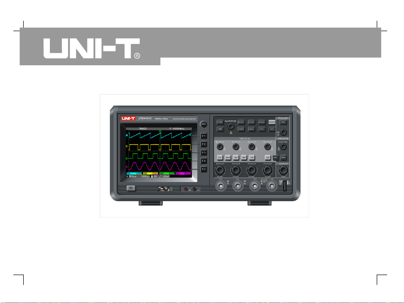
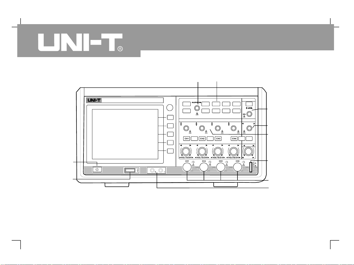
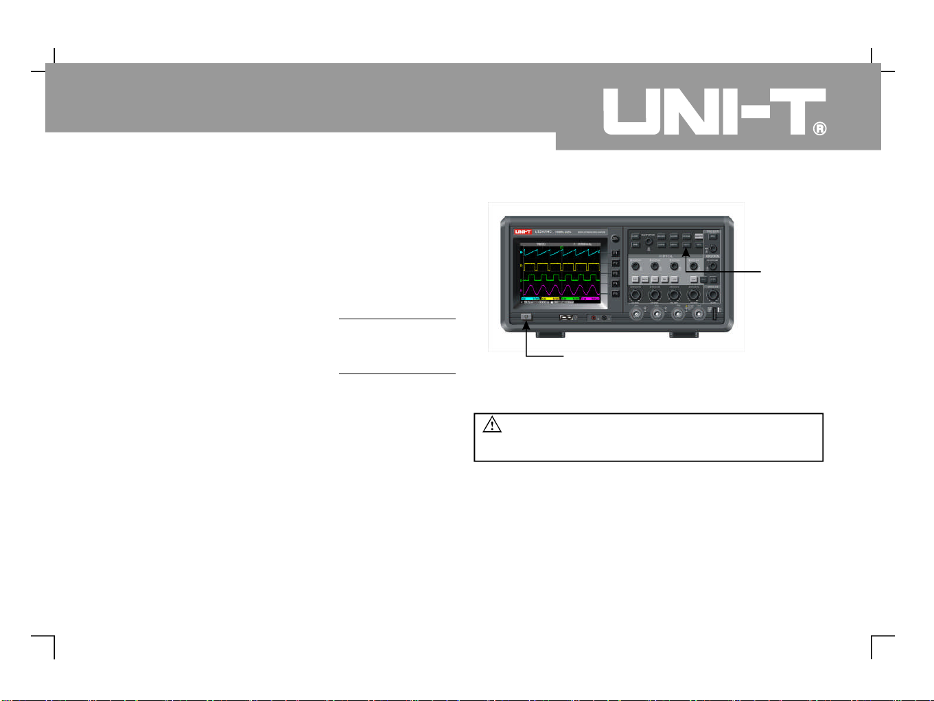
Figure1-1 Series Digital Storage Oscilloscope

UTD4000 Four-channel

User Manual

Page 12

UTD4000 Four-channel

User Manual

Figure 1-2 Back cover of UTD4000 four-channel digital storage oscilloscope

USB device communication

interface

External trigger

channel

Page 13

PROBE

COMPVMHz≈31All Inputs

400Vp Max

CAT II

1M 1 6pF

≈

TRIG GER

HOR IZONTAL

SCALE

HELP

REF

MATH

F1F2F3F4F5

ON/OF F

DMM

MEASURE

CURS OR

ACQ UIRE

DISP LAY

STOR AGE

RUN/STOP

UTIL ITY

AUTO

VERT ICAL

SCALE

SEC/ DIV

UTD4304C

300MHz 2GS/s

DIGITA LSTO RAGE OSCILLO SCOPE

POSI TION

POSITION

POSI TION

UTD4000 Four-channel

User Manual

Figure1-3 Series Digital Storage Oscilloscopes

Front Panel

UTD4000 Four-channel

Trigger controls

Horizontalcontrols

Frequently

UsedMenus

Multifunction

knob

Verticalcontrols

Probecompensation

signaloutput

Analogsignal input

USBHost

interface

ultim

eterinput

Powerswitch

Page 14

UTD4000 Four-channel

User Manual

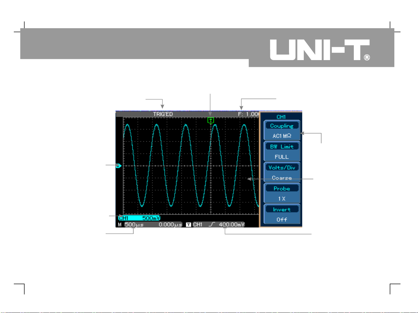
Figure1-4 Schematic diagram ofthedisplayinterface

Trigger status display

Displayingthehorizontal triggerposition

Trigger frequency counter

Channel vertical

attenuation range

Trigger level

Waveform

displaywindow

Themenuvaries with

individualfunctionkeys

Channel vertical

reference

Displaying main

time base setup

Page 15

UTD4000 Four-channel

User Manual

General Inspection

Functional Check

We suggest checking your new UTD4000 Four-

channel oscilloscope in the following steps.

If the package carton or foam plastic protective lining

is seriously damaged, please arrange for exchange

immediately.

A checklist of accessories that come with your

UTD4000 Four-channel oscilloscope is provided in

the section Accessories for UTD4000 Four-channel

Digital Storage Oscilloscopes of this user manual

Please check any missing items against this list

If any item is missing or damaged please contact

your NI-T dealer or our local office.

If the exterior of the unit is damaged, or it is not

erating normally, or it fails to pass the performance

test, please contact your UNI-T dealer or our local

office.

In the event of any shipping damages, please retain

the packaging and notify our shipping department or

your UNI-T dealer. We will be glad to arrange

maintenance or repair.

Carry out a quick functional check in the following

steps to make sure your oscilloscope is operating

normally.

1. Check the unit for possible shipping damages

2. Check the accessories

3. Thorough inspection of the entire unit

“

” .

.,U

Page 16

1. Power on the unit

UTILITY

UTILITY F1 F5

CH1

Power on the unit. AC power supply voltage range is

100V to 240V, frequency 45Hz-440Hz. After

connecting to power, start the self calibration process

on the optimal oscilloscope signal path at greatest

measurement accuracy. Press the [ ] button

and [ ] twice, then press the

control knob to perform the function Press

[ ] and [ ], then press [ ] to go to the next

page. There, press [ ] then the

control knob To recall default setup, see

Figure 1-5.

At the end of the above process, press [ ] to enter

the CH1 menu..

MULTIPURPOSE

Utility key

Power switch

Figure1-5

Warning

To avoid danger, ensure the digital

storage oscilloscope is safely grounded.

UTD4000 Four-channel

User Manual

Page 17

2. Accessing signals

Your UTD4000 Four-channel digital storage

oscilloscope has four input channels and an external

trigger input channel, as shown in Figure 1-6. Please

access signals in the following steps :

Connect the probe of the digital storage

oscilloscope to the CH input terminal and set

the attenuation switch of the probe to X

Figure

①

( - ) .

1101 7

Figure1-6

Four-channel input and external

trigger channel

EXT external trigger channel

–

Figure 1-7 Setting the attenuation switch of

the oscilloscope probe

UTD4000 Four-channel

User Manual

Page 18

②

: [ ] [ ]

You have to set the probe attenuation factor of

the oscilloscope. This factor changes the vertical

range multiple to ensure the measurement result

correctly reflects the amplitude of the signal being

tested Set the attenuation factor of the probe as

follows Press then to show X on

the menu

F F

4 2

AUTO

CH1 CH2

Connect the probe tip and ground clamp to the

connection terminal for the probe compensation

signal. Press [ ] and you will see a square wave

in the display (1kHz, approximately 3V, peak-to-peak

value) in a few seconds, as shown in Figure 1-

Press [ ] twice to close CH1, then press [ ]

to activate CH2 and repeat steps 2 and 3. Use the

same method for CH3 and CH4.

③

④

Figure1-8 Settingthedeflectionfactor

ofthe oscilloscope probe

Figure1-9 Probecompensationsignal

Proberation

UTD4000 Four-channel

User Manual

Page 19

ProbeCompensation

When connectingthe probeto any input channel for thefirst

time, perform this adjustment to match the probe to the

channel. Skipping the compensation calibration step will

result in measurement error or fault. Please adjust probe

compensationasfollows:

1 Setthe probeattenuationfactorto10X.Movethe switch

on the probe to 10X and connect the probe to CH1.

When using a hook-tip, ensure it is well connected to

the probe. Connect the probe tip to the output terminal

of the probe compensator s signal connector, and the

ground clamp to the ground cable connector of the

probecompensator.Acti

vateCH1then press [ ].

3. Ifyouseean Undercompensation or

Overcompensation waveform display adjust the

adjustable capacitance tab of the probe with a

screwdriver with non metal handle until a Correct

Compensation waveform shown in the above figure is

displayed

AUTO

“ ”

“ ” ,

- , “

”

2. Observe the displayed waveform.

Overcompensation

CorrectCompensation

Undercompensation

Figure1-10 Probecompensationcalibration

Warning :

, '

To avoid electric shock when measuring high

voltage with the probe ensure the probe s

insulation lead is in good condition. Do not

touch the metal part of the probe when

connectedtoHV power.

UTD4000 Four-channel

User Manual

Page 20

Automatic Setup for Waveform Display Getting to Know the Vertical System

Your UTD4000 Four-channel digital storage

oscilloscope features an auto setup function. It can

automatically adjust the vertical graticule factor,

scanning time base and trigger mode based on the

input signal, until the most appropriate waveform is

displayed. The auto setup function can only be

operated when the signal to be measured is 50Hz or

above and the duty ratio is larger than 1%.

1. Connect the signal to be tested to the signal input

channel.

2. P r es s [ ]. Th e o s ci l l os c o p e w i l l

automatically set the vertical graticule factor

scanning time base and trigger mode Should

you require to m

ake more detailed check you

can adjust manually after the auto setup

process until you get the optimal waveform

display

As shown in the figure below, there are a group of

buttons and knobs in the vertical control zone. The

following exercise will guide you through vertical

setup.

,.,

Using the Auto Setup Function :

A U T O

Figure1-11

Vertical control zone on the front panel

UTD4000 Four-channel

User Manual

Page 21

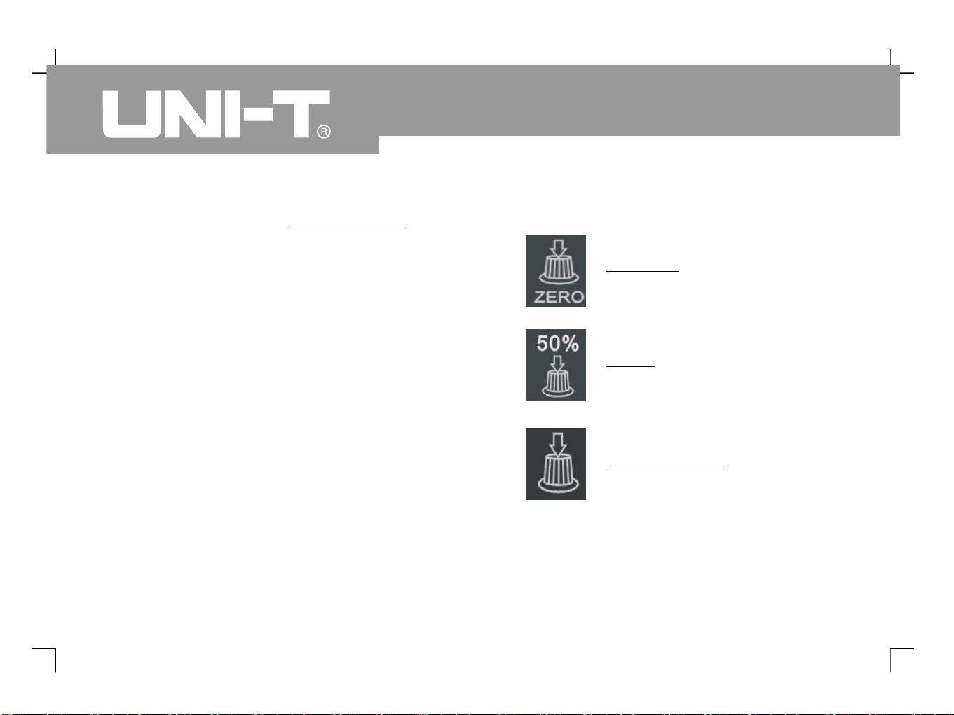
The knob can move the waveform

vertically. Press this knob to quickly return to the

centre point

Press the [ ], [ ], [ ], [ ], [ ] and

[ ] keys for the vertical channel operation menu,

or to open or close the waveform display channel.

Use the [ ](CH1, CH2, CH3, CH4) key to

set the vertical graticule factor.

Displacemen t and v er tical gr aticule facto r

adjustments of [ ], [ ] channels by

control knob

1. Press the vertical knob to display

the waveform signal in the centre of the window.

The vertical knob controls the

vertical display position of the signal When

you turn the vertical knob the

reference sign ind

icating the channel

level will move up and down with

the waveform

POSITION

MULTIPURPOSE

POSITION

...,[ ]

CH1 CH2 CH3 CH4 REF

MATH

VOLTS/DIV

REF MATH

GROUND

2. Change the vertical setup and observe changes

of status information. You can identify changes of

any vertical range by reading the status display

column at the lower corner of the waveform

window. Turn the vertical knob to

change the vertical range You will

find that the range in the current status

column has changed accordingly Press

and the screen will show the corresponding

operation menu, sign, waveform and range status

information.

/ .

. [ ],

[ ], [ ] , [ ] , [ ] [ ]

VOLTS/DIV

VOLT DIV

CH1

CH2 CH3 CH4 REF MATH

UTD4000 Four-channel

User Manual

Measurement Tips :

If the channel coupling is DC, you can measure the

signal s DC component quickly by checking the

distance between the waveform and signal

ground level

In the case of AC coupling, the DC of the

signal will be blocked. With this coupling mode you

can display the AC of the signal with

higher sensitivity

'..

component

Page 22

Getting to Know the System

Horizontal

As shown in the figure below, there are one button

and two knobs in the horizontal control zone. The

following steps will get you familiar with horizontal

time base setup.

The knob can move all channels MATH

waveforms and REF waveforms horizontally Press

this knob to quickly return to the centre point

[ ] horizontal menu, to display al

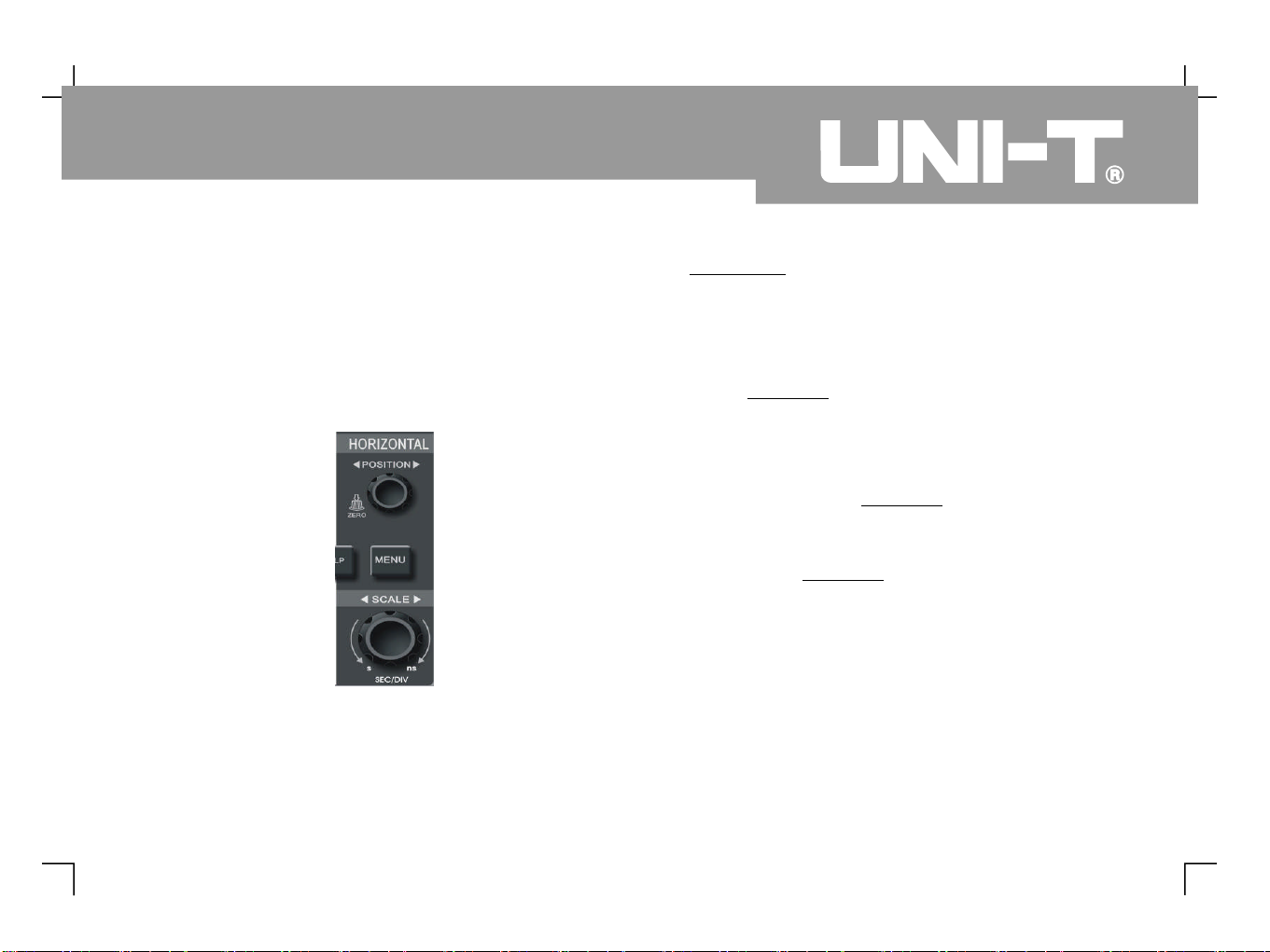
Use the knob to set the SEC DIV

graticule factor for horizontal scan If the window

is expanded you can adjust graticule of the

window there

1. Use the horizontal knob to change the

horizontal time base setup and check any

changes in status information. Turn the

horiz

ontal knob to change the

time base range You will find that

the time base range in the current status

column has changed accordingly Range of

horizontal scanning rate is 5ns/div~50s/div

(UTD4104C), in steps of 1-2-5

POSITION

SEC/DIV

,..

/.,./ .

..* :

MENU Window Du

Xbase Holdoff

SEC DIV

Note Horizontal scanning time base

range of the

Series varies from model to model

UTD4000 Four-channel

Figure1-12

Horizontal control zone on the front panel

UTD4000 Four-channel

User Manual

Page 23

2. Use the horizontal knob to adjust

the horizontal position of the waveform

window. When the horizontal knob is

turned you can see that the waveform moves

horizontally with the knob

3. Press [ ] to activate the display window and

dual time base menu. In this menu press [ ] to

activate window expansion Then press

again to quit window expansion and return to

the main display screen For dual time base

setup press You can also set the

holdoff time with this menu by turning the

control knob

,.. [ ]

, [ ].

POSITION

MULTIPURPOSE

F1FF13

UTD4000 Four-channel

User Manual

Shortcut key for resetting the trigger point to

horizontal zero :

When the trigger point has shifted significantly away

from the horizontal centre point, use the [POSITION]

knob to quickly reset the trigger point to the

horizontal centre point. You can also use the

horizontal knob for adjustments

POSITION

Definition

Trigger point

Holdoff

means the actual trigger point relative

to the centre point of the storage device. By turning

the horizontal knob you can move the

trigger point horizontally

means time before another

trigger to be accepted. Turn the

control knob to set the holdoff time By adjusting

holdoff time you can observe complex or

complicated signals

POSITION

MULTIPURPOSE

,..,.

the interval

Page 24

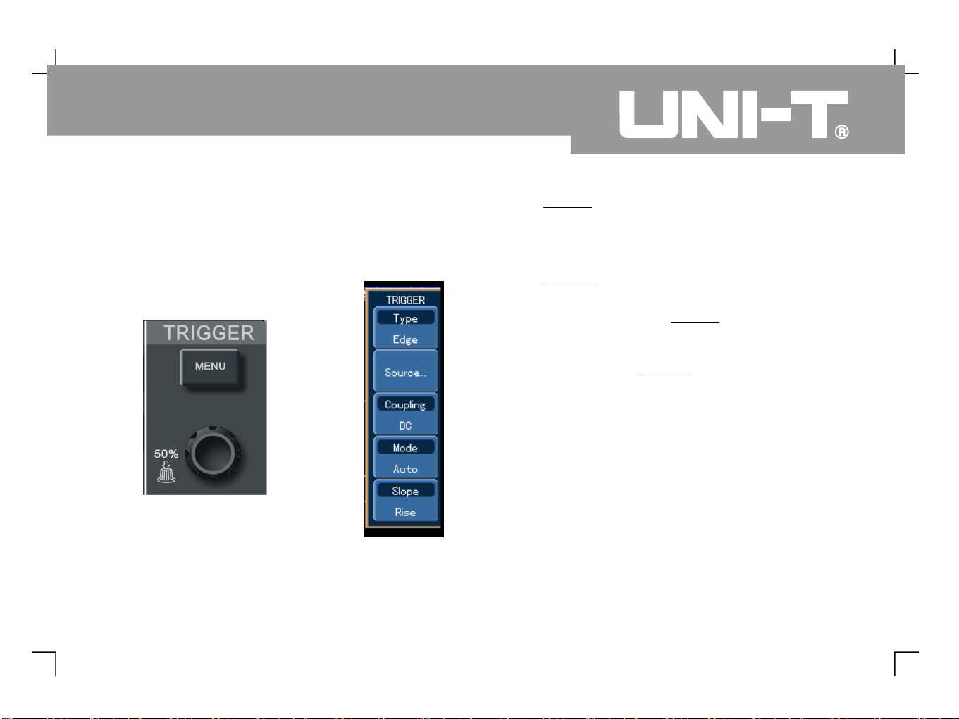
Getting to Know the Trigger System

As shown in Figure there are one knob and

one button in the trigger menu control zone. The

following steps will get you familiar with trigger setup.

Trigger knob

When operating edge, pulse width and slew rate

triggers, set the amplitude to be crossed by the

waveform upon signal occurrence by turning the

trigger knob To quickly set the trigger

level as the vertical centre point of the trigger

signal press the trigger knob

To display trigger menu contents

1. Use the trigger knob to change the

trigger level You will see a trigger sign on the

screen that indicates the trigger level The sign

will move up a

nd down with the knob While you

move the trigger level you will find the trigger

level value on the screen changing accordingly.

2. Open the trigger [ ] key (see the figure 1 )

to change trigger setup.

Press [ ] twice and select for

- ,

:., .

[ ]

...,[ ].

1 13

LEVEL

F1 EDGE TYPE

-14

UTD4000 Four-channel

User Manual

Figure1-13

Trigger menu on

the front panel

Figure1-14

Trigger Menu

Page 25

Press [ ] and select for [

] (Turn the control

knob to select and then press that key to

confirm).

Press [ ] then [ ]. Set for

Press [ ] then [ ]. Set for [ ].

F2 CH1 SIGNAL

SOURCE

F3 F1 DC COUPLING

F4 F1 AUTO MODE

F5 F2 RISE SLOPE

MULTIPURPOSE

[ ] .

Notes :

UTD4000 Four-channel

User Manual

Ic o n uti l i ty fu n c tion o f the

knob. Press this key to

quickly return to the centre point.

POSITION

Icon utility function of the trigger

knob Press this key to

quickly return to horizontal ground

level, i.e. trigger zero level

LEVEL

Ic o n uti l i ty fu n c tion o f the

knob Press

this key to confirm selection

MULTIPURPOSE

Page 26

Chapter 2

Instrument Setups

You should be familiar with basic operation of the

vertical controls, horizontal controls and trigger

system menu of your UTD4000 Series

oscilloscope by now. After reading the last chapter,

you should be able to use the menus to set up your

digital storage oscilloscope. If you are still unfamiliar

with these basic operation steps and methods, please

read Chapter 1.

This chapter will guide you through the following :

Four-channel

●●●●●●●●●●●

●

Settin g up the vertical system ([ ],

[ ],[ ], [ ], [ ], [ ],

Setting up the horizontal system ([ ],

Setting up the Trigger system ( ,

Setting up the sampling method ([ ])

Setting up the display mode

Storage and recall ([ ])

Setting up the help system ([ ])

Automatic measurement ([ ])

Cursor measurement ([ ])

Auto setup, run/stop key ([ ], [ ])

Multimeter ([ ])

Multipurpose control knob (

It is recommended that you read this chapter carefully

to understand the various measurement functions

and system operation steps of your UTD4000 four-

channel digital storage oscilloscope.

CH 1

CH2 CH3 CH4 MATH REF

ACQUIRE

DISPLAY

STORAGE

UTILITY

MEASURE

CURSOR

AUTO RUN/STOP

DMM

POSITION

VOLTS/DIV

POSITION SEC/DIV

TRIGGER MENU

LEVEL

MULTIPURPOSE

,), )

)

([ ])

)

UTD4000 Four-channel

User Manual

Page 27

Setting the Vertical System

CH1, CH2, CH3, CH4 and setups

CH1 CH2 CH3 CH4

Each channel has its own vertical menu. You should set up each item for each channel individually. Press the

[ ], [ ], [ ] or [ ] function button and the system will display the operation menu for CH1, CH2, CH3

or CH4. For explanatory notes please see Table 2 below

Table 2-1 Explanatory notes for channel menu

- :

：

UTD4000 Four-channel

User Manual

Function Menu

Setup

Explanatory Note

Coupling

DC 1M

AC 1M

GND

Pass AC and DC quantities of input signal. Intercept DC quantities of

the input signal.

Display reference ground level (without disconnecting the input signal).

BW Limit

Full

20MHz

Full band width.

Limit bandwidth to 20MHz to reduce noise display

VOLTS/DIV

Coarse

Fine

Coarse tune in steps of 1-2-5 to set up the vertical graticulefactor of

the vertical system Fine tune means further tuning within the coarse

tune setup range to raise the vertical resolution

Probe

10X

100X

1000X

Select either one value based on the probe attenuation factor to keep

the vertical deflection factor reading correct. There are four values :

1X, 10X, 100X and 1000X.

Invert

Off

Waveform is inverted

Normal waveform display.

Page 28

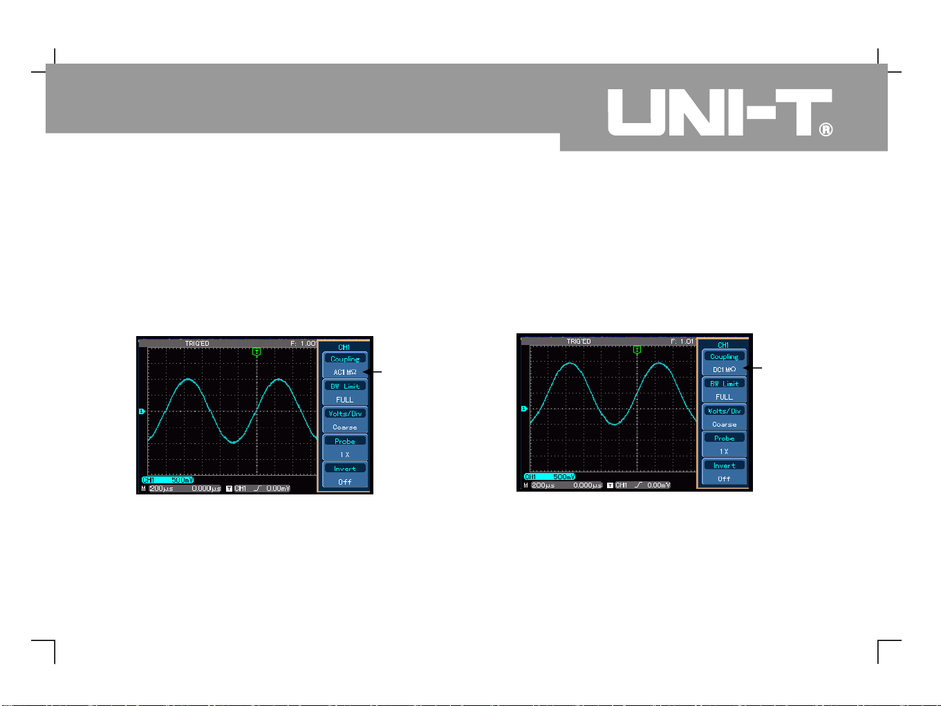
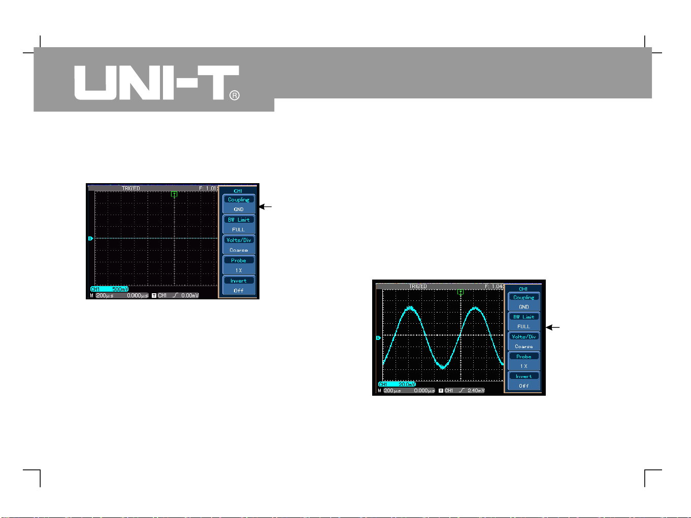
1. Setting up channel coupling :

F1 F2

Take an example of applying a signal to CH1. The

signal being tested is a sine signal that contains

DC%. Press [ ] to select AC then press [ ] to select

AC 1M It is now set up as AC coupling DC

quantities of the signal being tested will be

intercepted The waveform display is as follows

. .

. :

Press [ ] twice to select DC 1M Both DC and AC

quantities of the testing signal being inputted to

CH1 can pass through The waveform display is

as follows

..:

UTD4000 Four-channel

User Manual

Figure 2-1 DC quantities of the signal are intercepted

AC coupling

setup

DC coupling

setup

Figure 2-2 Both DC and AC quantities of the signal are

displayed

Page 29

UTD4000 Four-channel

User Manual

Press [ ] then [ ] to select ground. It is now set up

as ground. The waveform display is as follows :

F1 F3

* : ,

,..

Note In this mode although waveform is

not displayed the signal remains connected to

the channel circuit

2. Setting the channel bandwidth limit

CH1 F2

Take applying a signal to Ch1 as an example, the

signal to be tested contains high frequency

quantities.

Press [ ] to turn CH1 on, then press [ ] and [F1].

Bandwidth is now set to full bandwidth The signal

being measured can pass through even if it

contains high frequency quantities. The waveform

display is as follows :

Figure 2-3 Channel is set to ground mode

Ground coupling

setup

Figure 2-4 Waveform display at full

bandwidthdisplayed

Full

bandwidth

Page 30

Press [ ] then [ ]. The noise and high frequency

quantities over 20MHz of the signal being tested are

now restricted. Waveform display is as follows.

F2 F3

3. Setting up the probe rate

To match the probe attenuation factor setup, it is

necessary to set up the probe attenuation factor in

the channel operation menu accordingly For

example when the probe attenuation factor is

10:1 set the probe attenuation factor at 10X in

the channel menu Apply this principle to other

values to ensure the voltage reading is correct

The figure below shows the setup and vertical

range display when the probe is set at 10:1.

.,,..

UTD4000 Four-channel

User Manual

Figure 2-5 Waveform display when bandwidth

limit is on

Bandwidth

limit 20MHz

The BW bandwidth

limit icon

“ ”

Figure 2-6 Setting the probe attenuation factor in the

channel menu

Probe attenuation

factor

Vertical range

movement

Page 31

UTD4000 Four-channel

User Manual

4. Vertical VOLTS/DIV adjustment setup 5. Waveform inversion setup

You can adjust the VOLTS/DIV range of the vertical

deflection factor either in the coarse tune mode or

fine tune mode. In coarse tune mode the

VOLTS DIV range is 2mV/div~5V/div Tuning is in

steps of 1-2-5 In fine tune mode you can change

the deflection factor in even smaller steps within

the current vertical range so as to continuously

adjust the vertical deflection factor within the range

of 2mV/div~5V/div without interruption.

Waveform inversion : The displayed signal is inverted

180 degrees. Figure 2-8 shows the non inverted

waveform Figure 2-9 shows the inverted waveform

/ .

. ,

,-. .

Figure 2-7 Coarse tuning and fine tuning the vertical

Fine tune

setup

Vertical graticulefactor VOLTS/DIV movement

Figure Inversion setup for vertical channel

non inverted graticule factor

2-8

( )

Non-inverted

Page 32

Math functions are displays of and FFT

mathematical results of waveform channels CH1,

CH2, CH3 and CH4, and the digitally filtered

waveform.

The menu is as follows :

Operating Math Functions

+, - , ×,

UTD4000 Four-channel

User Manual

Figure 2-9 Inversion setup for vertical

channel (inverted)

Inverted

waveform

Waveforminversion icon

Figure Math functions

2-10

Math channel

range

Page 33

UTD4000 Four-channel

User Manual

Table 2-2a Explanatory notes for the Math menu (1)

Function Menu

Setup

Explanatory Note

Source 1

CH1

CH2

CH3

CH4

Set 1 as CH1 waveform

Set 1 as CH2 waveform

Set 1 as CH3 waveform

Set 1 as CH4 waveform

Source

Type

Math

To carry out functions

, ,

× ÷

＋－

, ,

Operator

Source Source 2

Source 1 Source 2

Source 1 Source

Source 1 Source 2

＋－×

12Source 2

CH1

CH2

CH3

CH4

Set 2 as CH1 waveform

Set 2 as CH2 waveform

Set 2 as CH3 waveform

Set 2 as CH4 waveform

Source

Next page 2/2

----

Go to next page

Page 34

UTD4000 Four-channel

User Manual

Table 2-2b Explanatory notes for the Math menu (2)

Function Menu

Setup

Explanatory Note

Compress

1/1

1/10

1/100

1/1000

Scale the waveform by ratio. There are four ratios to choose

from : 1/1, 1/10, 1/100, 1/1000

Y Offset

Use the control knob to move the waveform

vertically

MULTIPURPOSE

Y Level

----

Use the control knob to adjust the vertical

scale factor

MULTIPURPOSE

Pre 1/2

----

Return to previous page

----

Page 35

UTD4000 Four-channel

User Manual

FFT spectrum analysis

By using the FFT (Fast Fourier Transform algorithm

you can convert time domain signals YT into

frequency domain signals With FFT you can

conveniently observe the following types of

signals

Measure the harmonic wave composition and

distortion of the system

Demonstrate the noise characteristics of the DC

power

Analyse oscillation

) ,

( )

. ,

●●●

Figure FFT Frequency

2-11

Fundamental

frequency

component 1 MHz

Third harmonic

frequency

component 3MHz

FFT vertical

graticule unit mV

horizontal

graticule unit

Hz div

;

Page 36

UTD4000 Four-channel

User Manual

Table 2-3a Explanatory notes for the FFT menu (1)

Table 2-3b Explanatory notes for the FFT menu (2)

Function Menu

Setup

Explanatory Note

Source

CH1

CH2

CH3

CH4

Set CH1 as math waveform

Set CH2 as math waveform

Set CH3 as math waveform

Set CH4 as math waveform

Type

FFT

To carry out FFT algorithm functions

Window

Hamming

Blackman

Rectangle

Hanning

Set Hamming window function

Set Blackman window function

Set Rectangle window function

Set Hanning window function

Vertical coordinate

Linear

V dB

Set the vertical coordinate unit to linear or V dB

Next 2/2

----

Go to next page

Function Menu

Setup

Explanatory Note

Y Offset

----

Use the control knob to move the waveform

vertically

MULTIPURPOSE

Y Level

Use the control knob to adjust the vertical

graticule factor

MULTIPURPOSE

----

Pre 1/2

----

Return to previous page

----

Page 37

UTD4000 Four-channel

User Manual

Select the FFT Window

Assuming the YT waveform is constantly repeating

itself, the oscilloscope will carry out FFT conversion

of time record of a limited length. When this cycle is a

whole number, the YT waveform will have the same

amplitude at the start and finish. There is no

waveform interruption. However, if the YT waveform

cycle is not a whole number, there will be different

amplitudes at the start and finish, resulting in

transient interruption of high frequency at the

connection point. In frequency domain, this is known

as leakage. To avoid leakage, multiply the original

waveform by one window function to s

et the value to 0

for start and finish compulsively. For application of the

window function, please see the table below :

How to use FFT functions

Signals with DC quantities or DC offset will cause

error or offset of FFT waveform quantities. To reduce

DC quantities, select AC coupling To reduce

random noise and frequency aliasing resulted by

repeated or single pulse event set the acquiring

mode of your oscilloscope to average acquisition.

Page 38

UTD4000 Four-channel

User Manual

Table 2-4

FFT Window

Feature

Most Suitable Measurement Item

Rectangle

The best frequency recognition rate

the worst amplitude recognition rate

Basically similar to a status without

adding window

,..

Temporary or fast pulse. Signal level is generally

the same before and after. Equal sine wave of very

similar frequency. There is broad-band random

noise with slow moving wave spectrum.

Hanning

Frequency recognition rate is better

than the rectangle window, but

amplitude recognition rate is poorer.

Sine, cyclical and narrow band random noise

- .

Hamming

Frequency recognition rate is

marginally better than Hanning

window.

Temporary or fast pulse. Signal level varies greatly

before and after.

Blackman

The best amplitude recognition rate

and the poorest frequency

recognition rate.

Mainly for single-frequency signals to search for

higher-order harmonic wave.

Definition :

FFT recognition rate

Nyquist frequency :

.,,

means the quotient of the sampling and math points When math point value is

fixed the sampling rate should be as low as possible relative to the FFT recognition rate.

To rebuild the original waveform, at least 2f sampling rate should be used for waveform

with a maximum frequency of f. This is known as Nyquist stability criterion where f is the Nyquist

frequency and 2f is the Nyquist sampling rate.

Page 39

UTD4000 Four-channel

User Manual

Digital Filtering Function

Table 2-5a Explanatory notes for the digital filtering menu (1)

Figure Digital filtering

2-12

Setting the

maximum

frequency

Digital filtering

Function Menu

Setup

Explanatory Note

Source

CH1

CH2

CH3

CH4

Set CH1 as filter target

Set CH2 as filter target

Set CH3 as filter target

Set CH4 as filter target

Type

Filter

Digital filtering

Filter Type

Low-pass

High-pass

Band-pass

Set the filter to

low-pass filtering

Set the filter to

high-pass filtering

Set the filter to

band-pass filtering

Next 2/2

----

Go to next page

Page 40

UTD4000 Four-channel

User Manual

Table 2-5b Explanatory notes for the digital filtering menu (2)

Function Menu

Setup

Explanatory Note

Upper Limit

----

Effective only during low-pass filtering or band-pass filtering.

Use the control knob to set the maximum

frequency

MULTIPURPOSE

Lower Limit

----

Effective only during high-pass filtering or band-pass filtering.

Use the control knob to set the minimum

frequency

MULTIPURPOSE

Y Offset

----

Use the control knob to move the waveform

vertically

MULTIPURPOSE

Pre

1 /2

----

Return to previous page

Y Level

----

Use the control knob to adjust the vertical

graticule factor

MULTIPURPOSE

Page 41

UTD4000 Four-channel

User Manual

Reference Waveform

Display of the saved reference waveforms can be set

on or off in the REF menu. The waveforms are saved

in the non volatile memory of the oscilloscope or an

external USB device and are identified with the

following names : RefA, RefB. To display (Load) or

hide (off) the reference waveforms, take the

following steps

1. Press the [ ] key.

2. Press [ ] for Load and select the signal

source by turning the control

knob You can choose from 1 to 10 After

selecting a numeral for saved waveform e g

1 press the control knob to

confirm and the waveform originally stored in that

position can be recalled. For instructio

ns on

storing or recalling reference waveforms on the

USB device, read Storage and Recall

3. Press [F1] for RefB to select the second

signal source for the math function by repeating

step 2.

4. To close the reference waveform, press [ ].

In actual application, when using your UTD4000

to measure and observe such

waveforms, you can compare the current

waveform with the reference waveform for

analysis. Press to display the

reference waveform menu For setup please

refer to Table 2 6

: When [ ] is pressed after a waveform

is recalled or imported, that waveform will

remain.

. .

, . .

,.[ ]

- .

REF

OFF

REF

Note AUTO

MULTIPURPOSE

Four-channel

“ ”

Page 42

UTD4000 Four-channel

User Manual

Table 2-6a Explanatory notes for the REF menu (1)

Table 2-6b Explanatory notes for the REF menu (2)

Function Menu

Setup

Explanatory Note

Ref Wave

REF A

REF B

Select as the reference waveform

REF A

REF B

Load

Recall waveforms stored in 10 positions then select one with the

control knob Press the control knob to

confirm.

MULTIPURPOSE

----

To display the amplitude and time base contents of the current

waveform

Next 2/2

Go to next page

Function Menu

Setup

Explanatory Note

Y Offset

Use the control knob to move the waveform

vertically

MULTIPURPOSE

Y level

Use the control knob to adjust the vertical

graticule factor

MULTIPURPOSE

OFF

Close the reference waveform

Pre

1 /2

Return to previous page

Import

Enter the USB menu (see Table 2-7), recall the reference

waveform stored on the USB device

USB

Page 43

UTD4000 Four-channel

User Manual

Table 2-7 Explanatory notes for the USB menu

: To select an internal storage position, choose

between 1 and 10. In the case of external storage

device, plug in the USB device. A message saying

USB installation complete appears Press

on the next page for the import menu and then

enter the USB menu

In the USB menu use the key and

control knob to set the document

name Press to select the character

positions that need to be changed Use the

control knob to change the

selected characters or numerals

: Y Offset Y level OFF are

operative only after the reference waveform has

been recalled or imported

" " . [ ]

" " ,

: , [ ]

. [ ]

.., , [ ]

Note 1

Note 2 F1

Note 3 REF

MULTIPURPOSE

“ ” “ ” “ ”

Function Menu

Setup

Explanatory Note

File name

Use the control knob and F key to set

the document name to be imported from the USB device.

For specific operation instruction see note 2

MULTIPURPOSE

[ ]

1OKAfter confirming, go back to the REF menu. If there is such a

document on the USB device, it will be imported. Otherwise a

I/O failure message will appear

" "

Page 44

UTD4000 Four-channel

User Manual

Setting the Horizontal System

Horizontal Control

You can use the horizontal control knobs to change

the horizontal graticule (time base) and trigger the

horizontal position of the memory (triggering

position). Changing the horizontal graticule will cause

the waveform to increase or decrease in size relative

to the screen centre. When the horizontal position

changes, the position with respect to the waveform

triggering point is also changed.

Horizontal position : Adjust the horizontal positions of

channel waveforms (including math waveforms).

Resolution of this control button changes with the

time base.

Horizontal scaling : Adju

st the main time base, i.e

SEC/DIV. When time base extension is on, you can

use the horizontal scaling knob to change the delay

scanning time base and change the window width.

Two horizontal control knobs : Use the knob

to change horizontal time base graticule and use

the horizontal knob to change the

relative position if the triggering point on the

screen For instructions on how to display the

horizontal menu see Table

Horizontal controls menu : Horizontal menu display

(see the table below).

SEC/DIV

POSITION

,.[ ], .

2 8

Page 45

UTD4000 Four-channel

User Manual

Table 2-8 Explanatory notes for the horizontal menu

Represents the signal frequency currently

selected as trigger source.

Represents the triggering point position of the

current waveform.

Represents the trigger level of the current

waveform.

Distance between the triggering position and the

horizontal centre point.

The time base value of main time base M1, i.e

SEC/DIV.

Horizontal parameter interface definitions :

①②③④⑤

Function Menu

Setup

Explanatory Note

Window

Press [ ] to switch between the main screen and

expanded window

“ ”

Dual Xbase

Enter the dual time base menu. See Table 2-9

----

Holdoff

Use the control knob to adjust holdoff time

MULTIPURPOSE

96.0000ns~ 1.50000s

Figure 2-13 Horizontal parameter interface

⑤④③②①

Page 46

UTD4000 Four-channel

User Manual

Window Expansion

Window expansion can be used to zoom in a band of

waveform to check image details. Please refer to

Figure 2-14.

The window expansion setting cannot be slower than

the main time base setting. Maximum magnification

multiple is 100x.

In the window extension mode, the display is divided

into two zones as shown above. The upper part

displays the original waveform. You can move this

zone left and right by turning the horizontal

knob or increase and decrease the

selected zone in size by turning the horizontal

knob The lower part is the horizontally

expanded waveform Please note that the

recognition ra

te of expanded time base relative to the

main time base is now higher (as shown in the above

figure). Since the waveform shown in the entire lower

part corresponds to the selected zone in the upper

part, you can increase the extended time base by

turning the horizontal knob to decrease

the size of the selected zone In other words you

can increase the multiple of waveform expansion

POSITION

SEC/DIV

,..

. ,

Figure 2-14

Expanded screen display

Horizontally expanded section

Main window

waveform

Expanded

window

waveform

Page 47

UTD4000 Four-channel

User Manual

Dual Time Base Function

The dual time base function is similar to window

extension but there is a fundamental difference In

the window extension mode you can magnify the

waveform times whereas in the dual time

base mode you can magnify details of the

waveform being observed by thousands of times

In effect the main time base storage depth is

increased by thousands of times.

The dual time base menu and its operation are as

follows :

: The Math function is disabled in the dual time

base mode.

.,.

* Note

100

Figure 2-15 Dual time base

Delayed time

base M2

Main time

base M1

Page 48

UTD4000 Four-channel

User Manual

Table 2-9 Explanatory notes for the dual time base menu

Function Menu

Setup

Explanatory Note

Mode

Switching between main time base and dual time base

For dual time base mode instructions see Figure

2-1

M1 Base

Switch to the waveform displayed on a different channel. Only

one channel can be displayed in the dual time base mode

Main

Dual

X Adjust

When M1 is the main time base, use the horizontal and

knobs to adjust into main time base parameters

When M2 is the main time base, use the horizontal and

knobs to adjust into main time base parameters

POSITION

SEC/DIV

POSITION

SEC/DIV

M1M2CH1, CH2,

CH3, CH4

BACK

Return to the horizontal menu

M2 Shift

Set delayed time base M2 to move horizontally in escalating scale

Set delayed time base M2 to move horizontally in de-escalating scale

Coarse

Fine

Page 49

UTD4000 Four-channel

User Manual

Setting the Trigger System

Triggering decides when the oscilloscope collects

data and display waveforms. Once the trigger is

correctly set up, it can transform unstable displays

into meaningful waveforms. When beginning to

acquire data the digital storage oscilloscope first

collects sufficient data required for drawing a

waveform on the left side of the trigger point

When trigger is detected it continuously acquires

sufficient data to draw a waveform on the right

side of the trigger point

The trigger control zone on the operation panel of

your oscilloscope comprises a trigger knob

and a trigger button

: Edge, Pul

se , Video and Slope rate.

: Trigger is set to occur when the signal

is at the rising or falling edge. You can use the trigger

knob to change the trigger point s vertical

position on the trigger edge, i.e. the intersection point

of the trigger level line and the signal edge on the

screen.

When the pulse width of the

trigger signal reaches a preset trigger condition

trigger occurs

Carry out field or line trigger to

standard video signals.

Trigger condition is the signal rising

or falling rate.

Below are notes for various trigger menus.

For edge trigger menu setups please see Table

2-10

,.,.[ ] .

',.

LEVEL

Trigger Control

Trigger modes

Edge trigger

LEVEL

Pulse width trigger :

Video trigger:

Slope trigger:

Edge Trigger

Page 50

UTD4000 Four-channel

User Manual

Table 2-10 Edge trigger

Function Menu

Setup

Explanatory Note

Type

Edge

Coupling

Allow AC and DC quantities of the input signal to pass

Intercept DC quantities of the input signal

Reject low frequency quantities below 80kHz of the signal

Reject high frequency quantities above 80kHz of the signal

L/F Reject

H/F

Reject

Source

Set CH1, CH2, CH3 or CH4 as the signal source trigger signal

Set to external trigger or divide the external trigger source by 5

Set toAC power trigger

CH1 and CH2 trigger their respective signals alternately

CH3 and CH4 trigger their respective signals alternately

Ch1, CH2, CH3, CH4

EXT, EXT/5

LINE

CH1 & CH2

CH3 & CH4

Mode

The system automatically acquires waveform data when there is

no trigger signal . The scan baseline is shown on the display.

When the trigger signal is generated, it automatically turns to

trigger scan

The system stops acquiring data when there is no trigger signal.

When the trigger signal is generated, trigger scan occurs

One trigger will occur when there is an input trigger signal. Then

trigger will stop

Auto

Normal

Single

Continued table

Page 51

UTD4000 Four-channel

User Manual

Table 2-10 Edge trigger Connected to the table

Pulse trigger means determining the triggering time

based on the pulse width. You can acquire abnormal

pulse by setting the pulse width condition.

Table 2-11 Pulse width Trigger

( )

Pulse Trigger

Function Menu

Setup

Explanatory Note

Slope

Set to trigger at the signal s rising edge

Set to trigger at the signal s falling edge

Set to trigger at the signal s rising and falling edges

'''

Rise

Fall

Rise-Fall

Function Menu

Setup

Explanatory Note

Type

Pulse width Trigger

Source

Set CH1, CH2, CH3 or CH4 as the signal source trigger signal

Set to external trigger or divide the external trigger source by 5

Set toAC power trigger

CH1 and CH2 trigger their respective signals alternately

CH3 and CH4 trigger their respective signals alternately

Ch1, CH2, CH3, CH4

EXT, EXT/5

LINE

CH1 & CH2

CH3 & CH4

Page 52

UTD4000 Four-channel

User Manual

Table 2-11 Pulse width Trigger

Table 2-1 Pulse setup

Function Menu

Setup

Explanatory Note

Mode

The system automatically acquires waveform data when there is

no trigger signal. The scan baseline is shown on the

display. When the trigger signal is generated, it automatically

turns to trigger scan

The system stops acquiring data when there is no trigger signal.

When the trigger signal is generated, trigger scan occurs

One trigger will occur when there is an input trigger signal. Then

trigger will stop

Auto

Normal

Single

Pulse setup

See Table 2-12

Set the pulse width

Function Menu

Setup

Explanatory Note

Type

Pulse

Polarity

Set the positive pulse width as the trigger signal

Set the negative pulse width as the trigger signal

Positive

Negative

When

Trigger occurs when pulse width of the input signal is smaller

than the setting value

Trigger occurs when pulse width of the input signal is larger than

the value

Trigger occurs when pulse width of the input signal equals to the

value

setting

Page 53

UTD4000 Four-channel

User Manual

Table 2-1 Pulse width setup

By selecting video trigger, you can carry out field or

line trigger with NTSC or PAL standard video signals.

See Table 2-13 for the trigger menu :

Table 2-13 Video trigger

Video Trigger

Function Menu

Setup

Explanatory Note

Type

Pulse width

Setting

Set pulse width trigger to 20.0ns-10s with the

control knob

MULTIPURPOSE

Back

Return to the pulse width trigger menu

----

Function Menu

Setup

Explanatory Note

Type

Video

Source

Set CH1, CH2, CH3 or CH4 as the signal source trigger signal

Set to external trigger or divide the external trigger source by 5

Set toAC power trigger

CH1 and CH2 trigger their respective signals alternately

CH3 and CH4 trigger their respective signals alternately

Ch1, CH2, CH3, CH4

EXT, EXT/5

LINE

CH1 & CH2

CH3 & CH4

Video setup

See Table 2-1

Enter the video setup

Page 54

UTD4000 Four-channel

User Manual

Table 2-14 Video Setup

When PAL is selected for video and synchronization

mode is line, you will see a screen display as shown in

Figure 2-16. When synchronization mode is field, you

will see a screen display as shown in Figure 2-17.

Function Menu

Setup

Explanatory Note

Standard

PAL

NTSC

Suitable for PAL video signals

Suitable for NTSC video signals

Sync

Set the video odd field to synchronized trigger

Set the video even field to synchronized trigger

Set the line signal to synchronize with trigger

Set synchronized trigger on the specified line and adjust by

turning the control knob lines for PAL

lines for NTSC

MULTIPURPOSE

: ;

625

525

Odd Field

Even Field

All lines

Line Num

Back

Return to video trigger menu

Figure 2-16 Video trigger : Line synchronization

Page 55

UTD4000 Four-channel

User Manual

Slope trigger

If slope trigger is selected, trigger occurs when the

signal s rising or falling rate meets the set condition.

For the trigger menu see Table 2-15 below

Figure 2-17 Video trigger : Field synchronization

Page 56

UTD4000 Four-channel

User Manual

Table 2-15 Slope trigger

Function Menu

Setup

Explanatory Note

Type

Slew rate

Coupling

Allow AC and DC quantities of the input signal to pass

Intercept DC quantities of the input signal

Reject low frequency quantities below 80kHz of the signal

Reject high frequency quantities above 80kHz of the signal

DCACL/F Reject

H/F

Reject

Source

Set CH1, CH2, CH3 or CH4 as the signal source trigger signal

Set to external trigger or divide the external trigger source by 5

Set toAC power trigger

CH1 and CH2 trigger their respective signals alternately

CH3 and CH4 trigger their respective signals alternately

Ch1, CH2, CH3, CH4

EXT, EXT/5

LINE

CH1 & CH2

CH3 & CH4

Mode

The system automatically acquires waveform data when there is

no trigger signal. The scan baseline is shown on the

display. When the trigger signal is generated, it automatically

turns to trigger scan

The system stops acquiring data when there is no trigger signal.

When the trigger signal is generated, trigger scan occurs

One trigger will occur when there is an input trigger signal. Then

trigger will stop

Auto

Normal

Single

Slope Setup

See Table 2-16

Enter slope setup

Page 57

UTD4000 Four-channel

User Manual

Table 2-16 Slew rate setup

Function Menu

Setup

Explanatory Note

When

Trigger occurs when the signal slew rate within the threshold is

greater than the set slew rate

Trigger occurs when the signal slew rate within the threshold is

smaller than the set slew rate

Trigger occurs when the signal slew rate within the threshold

equals to the set slew rate

<>=

Polarity

Select the rising edge within the threshold for trigger

Select the falling edge within the threshold for trigger

Rise

Fall

Slew rate

Set the slew rate value with the control knob

MULTIPURPOSE

Threshold

Low

High

High & Low

Change the low level value with the control knob

Change the high level value with the control knob

Change the high and low level value with the

control knob

MULTIPURPOSE

Back

Return to the slew rate trigger menu

Alternate Trigger

When alternate trigger is selected, the trigger signal will be present in two vertical channels. This triggering

mode is suitable for observing two signals of unrelated signal frequencies Alternate trigger can also be

used to compare pulse widths

Page 58

UTD4000 Four-channel

User Manual

Adjusting the Holdoff Time

You can adjust the holdoff time to observe

complicated waveforms (e.g. pulse string series).

Holdoff time means the waiting time for the trigger

circuit to be ready for use again when the

oscilloscope is restarted. During this time the

oscilloscope will not trigger until the holdoff is

complete. For example, if you wish to trigger one

group of pulse series at the first pulse, set the holdoff

time to the pulse string width as shown in Figure 2-18.

Table 2-1 Trigger holdoff menu

Figure 2-18 Use the holdoff function to synchronize

complicated signals

Function Menu

Setup

Explanatory Note

Window

Press [ ] to switch between the Main and

Extended

“ ”

Dual Xbase

Enter the dual time base menu. See Table 2-9

----

Holdoff

Use the control knob to adjust holdoff time

MULTIPURPOSE

96.0000ns~ 1.50000s

Page 59

UTD4000 Four-channel

User Manual

Operation

Operation tip

Definitions

Trigger source

Input Channel

External Trigger

EXT

EXT TRIG

EXT

1. Follow the normal signal synchronization

procedure and select the edge and trigger source in

trigger [ ]. Adjust the trigger level to make the

waveform display as stable as possible.

2. Press the horizontal [ ] key to display the

horizontal menu.

3. Adjust the control knob in the

upper front panel The holdoff time will change

accordingly until the waveform display is stable

: Holdoff time is usually slightly shorter

than the Large cycle When observing a Rs232

communication signal waveform it is easier to

observe if holdoff time is slightly longer than the

starting edge time of every data fram

1. The signal used for trigger.

The signal for trigger can be obtained from

various sources : input channel (CH1, CH2, CH3,

CH4), external trigger EXT EXT/5 and LINE

etc

The most common trigger

source is to select one of the four input channels.

The channel selected as trigger source can

operate normally whether the input waveform

is displayed or not

This trigger signal can be input

directly through the external trigger input terminal. For

example, you can use an external clock or the signal

from a circuit to be tested as the trigger source. The

trigger source uses the input terminal to

access ex

ternal trigger signals setup is enabled

when signal trigger level range is 0.8V to +0.8V. To

allow input of larger signal through external trigger, the

trigger signal is divided by 5 in the EXT/5 mode, so that

the trigger level range is extended to 4V to +4V.

...,:

( , ) ,

.:.:.

MULTIPURPOSE

■

–

“ ”

Page 60

UTD4000 Four-channel

User Manual

■■■■■■■

■

LINE

Trigger mode

Auto Trigger

Note :

Normal Trigger

Single Trigger

Trigger coupling

DCACLF Reject

HF Reject

: .

. ..::.

: ,

[ ]

:....

means the AC power source This

trigger mode is suitable for observing signals

related to the AC power e g the correlation

between lighting equipment and power source

equipment to achieve stable synchronization

2. Determine the action of your

oscilloscope at trigger. This oscilloscope offers three

trigger modes for selection : auto, normal and single.

The system will acquire and

display waveform data automatically when

there is no trigger signal input When the

trigger signal is generated, it automatically turns

to trigger scan for signal synchronization.

Time base of the scan range can b

e set to

50ms/div or slower to generate a roll waveform.

In this mode your

oscilloscope samples waveforms only when

triggering conditions are met. The system stops

acquiring data and waits when there is no trigger

signal. When the trigger signal is generated,

trigger scan occurs.

In this mode you only have

to press the RUN button once and the

oscilloscope will wait for trigger. One sampling

will occur and the acquired waveform will be

displayed when the digital storage oscilloscope

detects a trigger. Then trigger will stop.

3. Trigger coupling determines

which quantities of the signal are tr

ansmitted to

the trigger circuit. Coupling modes are DC, AC,

low frequency suppression and high frequency

suppression.

:Allowing all quantities to pass

:Intercepting DC quantities and attenuating

signals under Hz

:Intercepting DC quantities and

attenuating low frequency quantities under

kHz

:Attenuating high frequency

quantities over kHz

108080

Page 61

UTD4000 Four-channel

User Manual

4. Data sampled

before after triggering

The trigger position is typically set at the

horizontal center of the screen. In this case, you are

able to view 6 divisions of pretrigger and delay

information. Adjusting the horizontal displacement of

the waveform with the knob allows you to

see more pretrigger information. By observing

pretrigger data, you can see the waveform before

trigger occurs. For example, you can detect the glitch

that occurs when the circuitry starts. Observation and

analysis of trigger data can help you identify the

cause of glitch.

As shown below, [ ] button in the control

zone is the function key for the sampling system.

Press the [ ] key to pop out the sampling

setup menu. You can use this menu to adjust the

sampling mode.

/ .

Pretrigger/Delayed Trigger

ACQUIRE

POSITION

Setting the Sampling System

Figure 2-19 Function key for the sampling

Page 62

UTD4000 Four-channel

User Manual

Table 2-18 Sampling menu

By changing the acquisition setup, you can observe

the consequent changes in waveform display. If the

signal contains considerable noise, you will see the

following displays when average sampling is not

selected and when 32-time average sampling is

selected. For sampling waveform display please see

Figure 2-20 and Figure 2-21.

Function Menu

Setup

Explanatory Note

Acquisition

Ordinary sampling mode

Peak detect mode

Set to average sampling with display of the average number of

times

Envelop sampling

Normal

Peak

Average

Envelop

Average number of

times (In the

Average mode)

Set the average number of times in multiples of 2, i.e. 2, 4, 8, 16,

32, 64, 128, 256. To change the average number of times, use

the control knob shown on the left in

Figure 2-19

MULTIPURPOSE

Equivalent

ON/OFF

Turn the equivalent sampling mode on or off. In this mode, selecting

alternate trigger (e.g. CH1 and CH2) as the trigger source is

disallowed

----

2~256

Page 63

UTD4000 Four-channel

User Manual

Notes :

1. Use Real time sampling to observe single

signals

2. Use Equivalent sampling to observe high

frequency cyclical signals.

3. To avoid mixed envelop when observing a signal,

select Peak Detect To reduce random noise

of the displayed signal select average

sampling and increase the average number of

times in multiples of 2 i e selecting from 2 to

256

..,..

Figure 2-20 Waveform without average

Figure 2-21 Waveform when 32-time

Page 64

UTD4000 Four-channel

User Manual

Definitions :

Real time sampling

Equivalent sampling

Normal mode

Peak detect mode

Average mode

Envelop Mode

::.:.::..:.

Acquiring the data required in

one go. Maximum sampling rate is 2GS/s.

This is a repeated sampling

mode that allows detailed observation of repeated

cyclical signals In the equivalent sampling mode,

the horizontal pixel aspect ratio is 20ps higher than

the real time mode, i.e. 50GS/s equivalent.

Your oscilloscope acquires signal

samples at equal time intervals to reconstruct

waveform

In this acquisition mode, the

oscilloscope identifies the biggest and smallest

values of the input signals at each sampling interval

and use these values to display the waveform. In

effect, the oscillosc

ope can acquire and display

narrow pulse which would otherwise be omitted in the

sampling mode. Noise seems to be more significant in

this mode.

The oscilloscope acquires several

waveforms and take the average value to display

the final waveform You can use this mode to

reduce random noise

The oscilloscope acquires multi-

amplitude waveforms and calculate all sampling

points that synchronize with the triggering point. The

maximum and minimum values are then displayed

Page 65

UTD4000 Four-channel

User Manual

Setting the Display System

As shown below, the [ ] key in the control

zone is the function key for the display system.

Table 2-1 Display menu

Press the [ ] button to pop out the setup

menu shown below. You can use this menu to adjust

the display mode.

DISPLAY

Figure 2-22 Function key for the sampling

Function Menu

Setup

Explanatory Note

Format

Voltage relative to time (horizontal graticule) is displayed

There are two groups in X-Y display mode. The first group is CH1

for X input and CH2 for Y input. The second group is CH for X

input and CH for Y input.

YTXYType

Sampling points are linked for display

Sampling points are directly displayed

Vectors

Points

Page 66

UTD4000 Four-channel

User Manual

Table 2-1 Display menu

Function Menu

Setup

Explanatory Note

Graticule

Set the grid display mode of the waveform zone to full, grid,

or frame

Cross Hair

Full

Grid

Cross Hair

Frame

Persist

Waveform on the screen is refreshed at normal rate

Waveform on the screen is maintained for 1 second and then

refreshed

Waveform on the screen is maintained for 2 seconds and then

refreshed

Waveform on the screen is maintained for 5 seconds and then

refreshed

Waveform on the screen remains on display. New data will be

added continuously until this function is disabled

Auto

1s2s5s

Infinite

Intensity

In Fast ACQ mode intensity of the waveform can

be adjusted with the control knob

“ ” ,

MULTIPURPOSE

1~32

Page 67

UTD4000 Four-channel

User Manual

X-Y Mode Caution :

X-Y XY

X-Y

This mode offers two separate displays. The first

group is CH1 and CH2, i.e. CH1 signal input on the

horizontal axis (X axis) and CH2 signal input on the

vertical axis (Y axis). The other group is CH3 and

CH4, i.e. CH3 signal input on the horizontal axis (X

axis) and CH4 signal input on the vertical axis Y

axis as shown in Figure 2 23

In the normal mode, you can move figures

horizontally with the CH1 or CH3 knob

and move figures vertically with the CH2 or CH4

knob Adjust the dimension and shape

of XY figures with of the four channels

and turn the knob to improve the display

quality of the lissajous figure

Than

ks to the unique display feature, your

oscilloscope can display channel waveform and

lissajous figure concurrently. The UTD4000

series also offers the following functions :

Automatic measurement mode

Cursor measurement mode

Reference or math waveform

The following functions are disabled under X-Y mode:

Dual time base

Horizontal knob

(

), - .

,.,

POSITION

VOLTS/DIV

SEC/DIV

POSITION

Four-

channe

■■■■■

Figure 2-23 Waveform display in X-Y

Page 68

UTD4000 Four-channel

User Manual

Key points :

Display Type

Refresh Rate

Storage and Recall

STORAGE

:.:.'

Vector display fills the space

between adjacent sampling points in display. The dot

mode displays only the sampling points

Refresh rate is the number of

times the digital storage oscilloscope refreshes the

waveform display per second. The refreshing speed

affects the capability to observe signal movements

speedily.

As shown below, the [ ] button in the control

zone is the function key for the storage system

Press the [ ] button to display the storage

setup menu. You can use this menu to save

waveforms or setup status of the oscilloscope in the

internal memory or the USB device, and recall any

ored waveform through RefA (or RefB), or press

[ ] to recall the setup status. When the USB

device is inserted, you can store the oscilloscope s

waveform display in bitmap format on the USB device.

Figure 2-24 Function key for the sampling

system (storage)

Page 69

UTD4000 Four-channel

User Manual

Instructions :

Press [ to go to the type menu. There

are three types to choose from : Setting, Wave,

Bitmap.

1. Select Wave to go to the waveform storage

menu shown below (see Table 2-2 ). A stored

reference waveform can be recalled with the REF

menu (reference waveform, P 32). For specific

steps see the REF instructions.

Table 2-20 Storage Menu

About Internal and CSV formats : When

exporting a reference waveform to the USB

device you can select internal or CSV.

Internal waveforms can only be imported to the

oscilloscope in REF mode and cannot be displayed

on any other interface. CSV waveforms can be

opened in EXCE

L on a PC. It is a group of

voltage and time correlation 2D data.

STORAGE

Note

]," "

“ ” “ ”

“ ”

Function Menu

Setup

Explanatory Note

Type

Select a signal source waveform displayed on the screen

Wave

Source

Select waveform from CH1

Select waveform from CH2

Select waveform from CH3

Select waveform from CH4

CH1

CH2

CH3

CH4

Save

To save the reference waveform on the internal memory of the

oscilloscope, turn the control knob to select

the storage position and press the control

knob to confirm

MULTIPURPOSE

1~10

----

Export

Go to the USB menu

See Table 2-21

Page 70

UTD4000 Four-channel

User Manual

Table 2-21 USB menu

2. Select setup to enter the save setting menu.

See Table 2-22

Table 2-22 Save setup menu

Function Menu

Setup

Explanatory Note

Filename

Set the document name to be imported from the USB device with

the control knob and key For specific

steps see note

[ ] .

MULTIPURPOSE

2 ( 34)

Format

See note

CSV, Iternal

----OKAfter confirming, go back to the reference waveform storage

menu. If there is a USB drive it will be exported to the USB,

otherwise the prompt I/O operation failed will appear

“ ”

Function Menu

Setup

Explanatory Note

Type

Save the current front panel setup status

1~10

Save

To save on the internal memory of the oscilloscope, select a save

position with the control knob and press the

control knob to confirm

MULTIPURPOSE

Setup

Page 71

UTD4000 Four-channel

User Manual

Table 2-22 Save setup menu

Table 2-23 USB menu

Function Menu

Setup

Explanatory Note

Filename

Enter the document name to be imported from the USB device

with the control knob and key For

specific steps see note

[ ] .

MULTIPURPOSE

2 (P34)

----OKAfter confirming, go back to the save setup menu. If there is a

USB drive it will be exported to the USB, otherwise the prompt

I/O failure will appear when exporting a waveform

After confirming, go back to the save setup menu. If the document

exists on the USB it will be imported, otherwise the prompt I/O

will appear when importing a waveform

" "

( )

operation failed ( )

Function Menu

Setup

Explanatory Note

1~10

Load

Recall 10 internal save positions and select one of them with the

control knob Press the

control knob to confirm

MULTIPURPOSE MULTIPURPOSE

Import

Enter the USB menu

See Table 2-2

Export

Enter the USB menu

See Table 2-2

Page 72

UTD4000 Four-channel

User Manual

3. Select bitmap to enter the bitmap export menu

See Table 2-24

: A bitmap can only be exported to a USB device.

Table 2-24 Bitmap export menu

Table 2-25 USB menu

Note

Function Menu

Setup

Explanatory Note

Bitmap

Export the display waveform to the USB device in bmp format

Export

Enter the USB menu

See Table 2-2

----

Function Menu

Setup

Explanatory Note

Filename

Enter the document name to be imported from the USB device

with the control knob and F key For

specific steps see note P Default is UNIT bmp

MULTIPURPOSE

[ ]

1 .

2 ( 34). 0000

After confirming, go back to the save setup menu. If there is a

USB drive it will be exported to the USB, otherwise the prompt

I/O will appear

" "

operation failed

Page 73

Utility Function Setup

As shown below, the [ ] key in the control zone

is the function key for utility functions.

Press the [ ] key to pop out the setup menu for

utility functions.

UTILITY

Figure 2-25 Function key for the sampling

system (function)

UTD4000 Four-channel

User Manual

Page 74

UTD4000 Four-channel

User Manual

Table 2-26 Utility menu 1

( )

Function Menu

Setup

Explanatory Note

Configure

Run auto system calibration

Display information like oscilloscope model, version and serial

number

Clear all saved reference waveforms and setups

Enter date and time setup. See Table 2-

Restore factory setup. See Appendix D

Set the auto function. See Table 2-

Return to the Utility menu

Self Cal

Version

Erase

RTC Setup

Next 2/2

Default Set

Auto setup

Pre1/2

Back

Preference

Select your desired languages with the

control knob and then press the control

knob to confirm

Classical, Traditional, Modern

Set the waiting time for automatic menu shutoff s s s

and manual Manual means automatic shutoff is disabled

Press to turn it on or off

Adjust the brightness of the display grid with the

control knob

Return to the Utility menu

MULTIPURPOSE

, ,

. .

[ / ]

5 10 20

MENU ON OFF

Language

Skin

Menu Display

Brightness

Back

Record

See Table 2-

Set waveform recording operation

----

Next 2/2

Setup

Go to the next page

Page 75

UTD4000 Four-channel

User Manual

Table 2-27 Utility menu 2

The Cymometer counts the frequency of trigger

events of the trigger channel. It works on edge or

pulse trigger but not alternate trigger. The

Cymometer is also disabled for video trigger

( )

Note :

Function Menu

Setup

Explanatory Note

Cymometer

Displayed at the top right corner of the screen when turned on.

See note

Set GPIB and LAN for communication.Applicable for optional

accessory UT-M06

ON/OFF

Interface

Pre

2/2

Return to the previous page

----

Go to the next page

----6667

Page 76

UTD4000 Four-channel

User Manual

Table 2-28 Waveform record menu

Function Menu

Setup

Explanatory Note

■

F(4)

Stop recording

Playback button

1. When you press this button the system plays back and

displays the number of screens to be played back. By turning

the control knob you can suspend

playback Turn the knob to select display of waveforms in

random screen numbering

2. If you wish to continue full playback, press [F4] to stop and

then press [F3]

MULTIPURPOSE

F(3)

Record button. Press this button then the [MENU ON/OFF] key

to record. The number of screens recorded is displayed. You

can record up to 100 screens of data Recorded data will be

lost when the oscilloscope is powered off This function

is disabled in dual time base roll average and envelop

modes

.., ,

●

F(5)

Page 77

UTD4000 Four-channel

User Manual

Table 2-29

Table 2- Auto setup menu

（）

RTC setup Real Time Clock

Function Menu

Setup

Explanatory Note

Display

Turn on the time display. Time display is disabled when the frequency

counter is in use

Press [ ] to select minute or hour, then adjust with the

control knob

MULTIPURPOSE

Min&Hour

On/Off

Press [ ] to select date or month, then adjust with the

control knob

MULTIPURPOSE

Day&Mon

Press [ ] to select and adjust with the control knob

MULTIPURPOSE

Year

Confirm your setting and return to the Utility menu

Function Menu

Setup

Explanatory Note

Channel

In the mode, default status is restored. The default status is as follows :

Bandwidth limit : full bandwidth VOLTS DIV coarse tune Inversion Off

unlock

; : ; :

In the mode, default status is restored. The default status is as follows :

Sampling mode : normal sampling equivalent sampling Off

unlock

; :

Acq set

Locked/Unlock

In the mode, default status is restored. The default status is as follows :

Type edge signal source adjusted see note trigger coupling DC

slew rate type rising

unlock

: ; : , ; : ;

Trigger

Unlock :

Channel is open/closed depending on the presence of input

signal Locked : Channel is maintained open or closed

Signal

Return to the Utility menu

Back

Locked/Unlock

Page 78

UTD4000 Four-channel

User Manual

Unlock

Locked

Notes :

Auto Calibration :

UTILIITY

: In Auto mode the setup will go back to

default for auto setup.

: In Auto mode the current status is locked for

auto setup.

For unloc or locked status see the table below 2-30.

The adjustment basis for the trigger signal source in

Auto mode :

1. If there is input signal in only one channel, that

channel will be the trigger source.

2. When more than one channels have input signal,

the system will search for trigger signal from CH1.

The first channel where signal is detected will be

the trigger source.

3. If no signal is detected in any channel, CH1 will be

the trigger source

You can correct measurement

erro

rs caused by environmental changes with the

auto calibration function. This process can be run

selectively when necessary. To make calibration more

accurate, power on your oscilloscope and allow 20

minutes to warm up. Then press the [ ] button

(help function) and follow on-screen instructions.

Important Points :

Page 79

UTD4000 Four-channel

User Manual

Automatic Measurement

MEASURE

Measurement menu

MEASURE]

As shown below, the [ ] key is the function

key for auto measurement. Read the following

instructions to familiarize with all the powerful

automatic measurement functions of your UTD4000

Four channel digital storage oscilloscope

Operation : Press [ to display 4 function

options, as shown in Table 2-

Table 2- Measurement menu

- .

31 (1)

Figure 2-26 Function key for the sampling

system (auto measurement)

Function Menu

Setup

Explanatory Note

All

Display all parameters. To quit all parameters press any key or knob

Press [ ] then use the control knob to select the

desired parameter Press the control knob to confirm

Up to 4 parameters can be displayed on screen simultaneously i e

parameter to parameter from left to right

. .

, . .

MULTIPURPOSE

1 4

Custom

Visual indication of the measurement value s physical properties by lines.

Turn on the indicator and select between parameters 1 and 4

Indicators

Clear all customized parameters

Clear

Enter the next page

Next 2/2

Page 80

UTD4000 Four-channel

User Manual

Table 2- Measurement menu

Table 2- Delay menu

32 (2)

Function Menu

Setup

Explanatory Note

ADV

The rising edge or falling edge time interval of a random channel

waveform. See Table 2-33

Delay

Phase

----

Confirm your setting and return to the Utility menu

Pre 2/2

Function Menu

Setup

Explanatory Note

From

Select one channel waveform as the delayed reference waveform

Take the centre point of 10%-90% of the waveform rising or falling edge

From edge

CH1 CH

CH3, CH4

, ,

Select one channel waveform as the delayed measurement waveform

Take the centre point of 10%-90% of the waveform rising or falling edge

To edge

Selection of the measurement point of delayed measurement

waveform is complete Return to the measurement menu

Rise, fall

----

CH1 CH

CH3, CH4

, ,

Rise, falle

Page 81

UTD4000 Four-channel

User Manual

Note Automatic measurement of voltage parameters

Customised parameters are for quick parameter

measurement. The measurement menu of your

oscilloscope is capable of measuring 26 waveform

parameters. Two of them (delay and phase for

advance measurement) are generally used when you

do not require to measure all parameters but only a

few. You can set these as customized parameters.

Customized parameters are displayed on the screen.

Your UTD4000 Series Oscilloscope

can automatically measure the following voltage

parameters :

Peak-to-peak value (Vpp) : The voltage value from the

highest point to lowest point of the waveform.

Maximum va

lue (Vmax) : The voltage value from the

highest point to ground (GND) of the waveform.

Minimum value Vmin The voltage value from

the lowest point to ground GND of the waveform

Amplitude value (Vamp) : The voltage value from top

to base of the waveform.

Mean (Vmid) Half of the amplitude value.

Top value (Vtop) : The voltage value from the level top

to ground (GND) of the waveform.

Base value (Vbase) : The voltage value from the level

base to ground (GND) of the waveform.

Overshoot : The ratio value of the difference between

maximum value and top value to the amplitude value.

( ) :

( ) .

Four-channel

Figure 2-27 Measurement parameters

Page 82

UTD4000 Four-channel

User Manual

Preshoot : The ratio value of the difference between

minimum value and base value to the amplitude

value.

Average : Average amplitude of signals within 1 cycle.

Root mean square value (Vrms) : The effective value.

Energy generated by AC signal conversion during 1

cycle with respect to the DC voltage that produces

equivalent energy, i.e. root mean square value.

Your UTD4000 Series Oscilloscope

can automatically measure the frequency, cycle,

rising time, falling time, positive pulse width, negative

pulse width delay positive duty ratio negative

duty ratio and time parameters Definition

s of

these parameters are as follows

RiseTime : The time taken by the waveform amplitude

to rise from 10% to 90%.

FallTime : The time taken by the waveform amplitude

to fall from 90% to 10%.

Positive Pulse Width (+Width) : The pulse width when

positive pulse is at 50% amplitude.

Negative Pulse Width (-Width) : The pulse width when

negative pulse is at 50% amplitude.

Delay (Rising or falling edge) : Delayed time from

wa v e f o r m t o w a ve f o r m (d u r i n g ad v a n c e

measurement).

Positive duty ratio (+Duty) : Ratio of positive pulse

width to cycle.

Negative duty ratio (-Duty) : Ratio of negative pulse

width to c

ycle.

Automatic measurement of time parameters

Four-channel

, , ,

9 .

Page 83

UTD4000 Four-channel

User Manual

Cursor Measurement

CURSOR

Notes

Press [CURSOR] to display the measurement cursor

and cursor menu, then adjust the cursor position by

turning the control knob As

shown in the figure below in the

control zone is the function key for cursor

measurement

You can move the cursor to carry out measurement in

the [ ] mode. There are two modes to choose

from : voltage and time. When measuring voltage,

select voltage for type and adjust the positions of

the two cursors with the control

knob to measure V. Likewise, by selecting time you

can measure T. The [ ] menu has two other

modes : independent and tracking In the

independent mode you can adju

st the positions of

the two cursors independently In the tracking

mode you press the control knob

to move two cursors simultaneously

1. In the independent or tracking mode, select one of

the cursors with the control knob

The selected cursor is a solid line. Adjust its

position with the control knob

2. There are two percentage options. The current

status is 100%. The value between the two

cursors is set to 100% i e one cursor is 0%

and the other is 100% When 100% is set to 6

DIV the 3DIV area on the screen is 100%.

3. When the cursor function is enabled, measurement

value is automatically displayed in the

top left

corner. @ is the selected cursor value.

MULTIPURPOSE

, [ ]

.,.,.,...

, . .

, ±

Figure 2-27 Function key for the sampling

system (cursor)

Page 84

UTD4000 Four-channel

User Manual

Table 2- ime cursor measurement menu

Table 2- Voltage cursor measurement menu

34 T

Function Menu

Setup

Explanatory Note

Type

Measure time with the cursor

Time

Select time as the measurement parameter

Select frequency as the measurement parameter

Select percent as the measurement parameter

Select d as the measurement parameter

egree

V Units

Mode

Independent

Tracking

Move any one of the two cursors

Move two cursors simultaneously without changing T

△

Second

Hertz

Percent

Degree

Function Menu

Setup

Explanatory Note

Type

Measure voltage with the cursor

Amplitude

Select voltage as the measurement parameter

Select percent as the measurement parameter

H Units

Mode

Independent

Tracking

Move any one of the two cursors

Move two cursors simultaneously without changing V

△

Base

Percent

Page 85

UTD4000 Four-channel

User Manual

Using the Run Button

There is a button on the top right corner on the front

panel : [ ]. When this button is pressed and

a green indicator lights up, your oscilloscope is in a

running status. If a red light comes on after pressing

this key, it indicates the unit has stopped operation.

Acquire waveform continuously or stop acquisition.

If you want the oscilloscope to acquire waveform

continuously, press [ ] once. Press the

button again to stop acquisition. You can use this

button to switch between acquiring and stop acquiring

waveform. In the Run mode, a green light comes on

and AUTO appears on the screen. In the STOP mode

a red light comes on and STOP appears on the

screen.

RUN/STOP

Figure 2-28 RUN/STOP key

Page 86

UTD4000 Four-channel

User Manual

Auto Setup :

AUTO

As shown above, Auto Setup can simplify operation.

Press [ ] and the oscilloscope can automatically

adjust the vertical graticule factor and horizontal time

base range according to the amplitude and frequency

of the waveform, and ensure stable display of the

waveform. When the oscilloscope is in auto setup

mode, the system setup is as follows :

Function Menu

Setup

Acquire

Normal

Horizontal position

Display format

Automatically adjusted

SEC/DIV

Adjust according to signal frequency

Trigger coupling

Holdoff

Minimum value

Trigger level

Set at 50%

Trigger mode

Auto

Trigger source

Automatically adjusted. See notes to Table 2-30 for details

Trigger slope

Rising

Trigger type

Edge

BW Limit

Full

VOLT/DIV

Adjust according to amplitude of the signal

Table 2- Auto setup

Page 87

UTD4000 Four-channel

User Manual

Menu Display ON/OFF :

Multimeter Measurement

DMM

Notes :

Help System

Vertical Position Control

Note: HELP

“ ” ,

,..

To display or hide the current menu

With the menu ON/OFF key you can display or

hide the menu currently on screen but help

messages are not displayed

Operation instructions : Open the multimeter function

menu by pressing the [ ] (Digital Multimeter)

button.

If it is necessary to test electric current, follow these

steps :

Insert the current/voltage converter module (UT-M03 or

UT-M04) that comes with the oscilloscope into the

digital multimeter port, and move the switch of the

current/voltage converter so that it is consistent with the

selected DMM current. Proceed with testing.

Cautions :

. Please select a suitable current/voltage converter

module that fits the measurement range, and

select an appropriate range. If you are not certain

about the current being tested, make an

estimation, use the UT-M04(4A) which has the

largest range, then select a suitable module range

to suit the data.

2. The current-voltage converter module of the

multimeter cannot be used to measure AC current.

3. When measuring large current with the UT-M04

module, to ensure precision, carry out power on

measurement every 15 minutes Do not power

on for more than 15 seconds each time

The oscilloscope has a H

elp system with topics that

cover all the features of the oscilloscope. The

oscilloscope displays information about the last menu

displayed on the screen when you push the HELP

.Information about specific menus and controls, such

as the .

Push button to display or exit help

information

[ ]

Page 88

UTD4000 Four-channel

User Manual

Table 2- DMM Menu

Function Menu

Setup

Explanatory Note

Funtion

DMM functions on/off

ON/OFF

Mode

Voltage

Resistance

ON/OFF

Diode

DC current

Activate the voltage measurement function. Maximum measurement

value for DC voltage is 400V. Maximum measurement value for AC

voltage is 400V

Activate the resistance measurement function. Maximum measurement

value for resistance is 40M

Activate the on/off measurement function. When on/off measuring is

lower than 70 the beeper will sound

Activate the diode measurement function. Connect the positive pole to

the red , and the negative pole to the black test lead

Current range : 4mA, 40mA, 400mA, 4A

test lead

Win shift

Set the horizontal shift or vertical shift of the window with the

control knob

MULTIPURPOSE

Page 89

Chapter 3 Practical Example

Illustrations

Illustration 1 : Measuring simple signals

1. To quickly display this signal, follow the

steps below :

AUTO

2. Voltage and time parameters for automatic

measurement

MEASURE

MENU ON/OFF

To observe and measure an unknown signal, and to

quickly display and measure the signal s frequency

and peak-to-peak value.

In the probe menu, set the attenuation factor to

10X and set the switch on the probe to 10X.

Connect the CH3 probe to the circuitry point to be

measured.

Press [ ].

The oscilloscope will carry out auto setup to

optimise waveform display. In this status, you can

further adjust the vertical and horizontal range

until you get the desired waveform display.

Your oscilloscope can automatically measure

most display signals. To measure signal

frequency and peak-to-peak value, f

ollow the

steps below :

Press [ ] to display the automatic

measurement menu.

Press [ ] to enter the measurement type

selection menu.

Use the control knob to select

peak to peak value then press it down to

confirm Next use the control

knob to select frequency then press it down to

confirm

Press [ ] to exit the selection

menu.

- - ,

①②③④①②③

MULTIPURPOSE

UTD4000 Four-channel

User Manual

Page 90

UTD4000 Four-channel

User Manual

Peak-to-peak and frequency measurements will now

appear at the bottom of the screen, as shown in

Figure 3-1.

As in the previous scenario, set the probe attenuation

factor of the probe and oscilloscope channel to 10X.

Connect the CH1 to the circuit signal input terminal

Connect CH2 to the output terminal

Press [ ].

Continue to adjust the horizontal and vertical

range until you get the desired waveform display.

Press [ ] to select CH1. Adjust vertical

position of the CH1 waveform by turning the

vertical position control knob.

Press [ ] to select CH2. In the same way

described above, adjust vertica

l position of the

CH2 waveform so that the waveforms of CH1 and

CH2 do not overlap. This will make observation

easier.

Illustration 2 : Observing the delay caused by a

sine wave signal passes through the circuit

Steps :

1. To display CH1 and CH2 signals :

AUTO

CH1

CH2

①②③

④

Figure 3-1 Automatic measurement

Page 91

2. Observing the delay caused by a sine wave

signal passes through the circuit and observing

waveform changes.

MEASURE

F5F1F 1

. .

①②③

When measuring channel delay automatically :

Press [ ] to display the automatic

measurement menu. Press [ ] to enter next

measurement menu. Press [ ] for advance

m e a s u r e m e n t , the n [ ] f o r d e l a y e d

measurement.

In the delayed measurement menu, set

measurement from CH1, i.e. from waveform

edge "rising”, to Ch2, i e to waveform edge

"rising” Press OK to confirm.

"Delay” appears on the screen.

UTD4000 Four-channel

User Manual

Figure 3-2 Waveform delay

Page 92

UTD4000 Four-channel

User Manual

Illustration 3 : Acquiring single signals

RUN/STOP

The advantage and special feature of your digital

storage oscilloscopes lie in its ability to acquire non

cyclical signals like pulse and glitch. To acquire a

single signal, you must have transcendental

knowledge of that signal to set the trigger level and

trigger edge. For example, if the pulse is a logical

signal of TTL level, the trigger level should be set at

about 2V and the trigger edge should be set to rising

edge trigger. If you are not certain about the signal,

you can observe it by automatic or normal trigger to

determine the trigger level and trigger edge.

Steps :

1. As in the previous illu

stration, set the attenuation

factor of the probe and CH1.

2. Carry out trigger setup.

Press [ ] in the trigger control zone to

display the trigger setup menu.

In this menu, use F1~F5 menus to set the trigger

type to edge set trigger source to Ch1 set

trigger coupling to DC set trigger mode to

single and set slew rate type to rising

Adjust horizontal time base and vertical range to

an appropriate range.

Turn the knob to get the desired level.

Press [ ] and wait for a signal that

meets the trigger condition. If any signal reaches

the set trigger level, the system will sample once

and display it on the screen

. By using this

function you can easily acquire any occasional

event. For example, when a sudden glitch of

relatively big amplitude is acquired : set the

trigger level to just higher than the normal signal

level. Press [ ] and begin waiting.

When a glitch occurs, the machine will

automatically trigger and record the waveform

immediately before and after triggering. By

turning the horizontal knob in the

horizontal control zone on the front panel, you

can change the trigger position horizontally to

achieve negative delay trigger of various lengths

for easy observation of waveform occurring

efore the glitch.

, ,

①②③④⑤

LEVEL

POSITION

Page 93

Illustration 4 Reducing random noise of signals

If the signal being measured is stacked with random

noise, you can adjust the setups of your oscilloscope

to filter or reduce the noise, so it will not cause

interference to the signal during measurement.

(Waveform is shown below)

UTD4000 Four-channel

User Manual

Figure 3-3 Single signal

Figure 3-4 Reducing random noise of signals

Page 94

UTD4000 Four-channel

User Manual

Steps :

As in the previous illustration, set the

attenuation factor of the probe and Ch1.

Connect the signal to ensure stable display of

waveform.

Improving trigger by setting trigger coupling

Reducing display noise by setting the

sampling mode.

ACQUIRE

F1 F3

1.2.See the previous illustration for

operation instruction. See the previous chapter

for guidance on adjusting the horizontal time

base and vertical range.

Press [ ] in the trigger zone to display the

trigger setup menu.

Set trigger coupling to low frequency

suppression or high frequency suppression

By selecting low frequency suppression a

high pass filter is set up It filters low

frequency signal quantities under kHz and

allows high frequency signal quantities to

pass through If you select high frequency

suppression a low-pass filter is set up. It filters

high frequency signal quan

tities higher than

80kHz and allows low frequency signal quantities

to pass through. By setting low frequency

suppression or high frequency suppression

you can suppress low frequency or high

frequency noise respectively and achieve a

stable trigger.

If the signal being measured is stacked with

random noise and the waveform is too coarse as

a result, you can use the average sampling mode

to eliminate random noise display and reduce the

size of waveform for easy observation and

measurement. After getting the mean, random

noise is reduced and details of the signal are

clearer. Follow the st

eps below :

Press [ ] in the menu zone of the front

panel to display the sampling setup menu. Press

menu operation key [ ] then [ ] to set

sampling mode to AVERAGE, then press the

control knob to adjust the

average number of times in multiples of 2

..- .

80.,

①

②

MULTIPURPOSE

Page 95

i e 2 to 256 until you get the desired

waveform display that meets observation and

measurement requirements See the figure

below

Your oscilloscope can measure 28 waveform

parameters automatically. All auto parameters can be

measured with the cursors. By using the cursors, you

can quickly measure the time and voltage of a

waveform.

To measure the peak frequency of a Sinc signal,

follow the steps below :

1. Pr es s [ ] to display the cursor

measurement menu.

2. Press [ ] to activate the cursor measurement

function.

3. Press [ ] again to set cursor type to time

4. Press [ ] to set the vertical cursor unit t

o Hz

5. Turn the control knob to set

cursor 1 at the Sinc first peak

. . ,

. ()...

Illustration 5 : Using the cursors for measurement

I. Measuring the frequency of a Sinc peak

CURSOR

F1F1F3

MULTIPURPOSE

UTD4000 Four-channel

User Manual

Figure 3-5 Signal noise suppressed

Caution : In the average sampling mode the

waveform display will update at a slower rate.

This is normal.

Page 96

UTD4000 Four-channel

User Manual

6. Press the control knob to

select cursor 2 then turn the

control knob again to set cursor 2 at the Sinc

second peak See the figure below.

1. Pr es s [ ] to display the cursor

measurement menu.

2. Press [ ] to activate the cursor measurement

function.

3. Press [ ] again to set cursor type to time

4. Press [ ] to set the vertical cursor unit to ratio

5. Turn the control knob to set

cursor 1 at the first rising edge peak of the

pulse

6. Press the control knob to

select cursor 2 then turn the

control knob again to set cursor 2 at the

second rising edge peak of the pulse.

7. Press [ ]. Current position is 100%. Set the

curre

nt value between cursor 1 and cursor

2 to 100%

.....

MULTIPURPOSE

II. Measuring the negative duty ratio of a pulse

signal

CURSOR

F1F3F4

△

Note : When using the cursor to measure voltage,

follow step 2 only and set the cursor type to

voltage.

Figure 3-6 Using the cursors to test signal

frequency

Page 97

8. Use the control knob to set

cursor 1 at the first falling edge of the pulse

This value is the negative duty ratio.

See the figure below.

Measure the phase difference that occurs when a sine

signal passes through the circuit. Connect CH1 to the

input signal of the circuit and connect CH2 to the

output signal of the circuit. To make testing easier,

CH1 and CH2 displacements are set in the centre

point, as shown in Figure 3-8. Follow the steps below :

1. Pr es s [ ] to display the cursor

measurement menu.

2. Press [ ] to activate the cursor measurement

function.

3. Press [ ] again to set cursor type to time

4. P

ress [ ] to set the vertical cursor unit to Degree

5. Turn the control knob to set

cursor 1 at the center point of the first sine

rising edge where is crosses with channel

ground line

...().

MULTIPURPOSE

△

III. Measuring the phase difference between two

signals

CURSOR

F1F1F3

UTD4000 Four-channel

User Manual

Figure 3-7 Using the cursors to test pulse

negative duty ratio

Page 98

UTD4000 Four-channel

User Manual

6. Press the control knob to

select cursor 2 then turn the

control knob again to set cursor 2 at the

center point of the second rising edge

7. Press [ ]. Current position is 100%. Set the

current value between cursor 1 and cursor

2 to 100%

8. Press [ ], then [ ] to set the cursor at

the CH2 signal being tested. Keep cursor 1

stationary and move cursor 2.

9. Use the control knob to set

cursor 2 at the center point of the first rising edge

of the CH2 signal. This value is the phase

difference between the two signals

See the figure below.

...

MULTIPURPOSE

CH2 CURSOR

△

Figure 3-8 Using the cursors to test the

phase difference between two

signals

Page 99

Illustration 6 : Using the X-Y function

CH2

AUTO

DISPLAY

To check the phase difference between two channels.

Example : To measure the phase variation when a

signal passes through the circuit, connect your

oscilloscope to the circuit and monitor the input and

output signals. To check the circuit s input and output

in the X-Y coordinate mode, follow the steps below :

1. Set the attenuation factor of the probe to 10X. Set

the switch of the probe to 10X.

2. Connect the CH1 probe to the input terminal of

the network. Connect the CH2 probe to the

output terminal of the network

3. If the channel is not displayed, press the [CH1]

and [ ] menu button to enable the two

annels.

4. Press [ ].

5. Adjust the vertical knob to make the

displayed amplitude of the two channels to

about equal

6. Press the [ ] menu key to recall the

display menu.

7. Press [ ] to select X-Y The oscilloscope will

display the circuit s input and output

characteristics in a Lissa jous figure.

8. Adjust the vertical scale and vertical position

knob to achieve the best result of waveform.

9. Using the elliptic oscilloscope display graph to

observe, measure and calculate the phase

difference.

see the figure below

'...'

( )

SCALE

UTD4000 Four-channel

User Manual

Figure 3-9

Signalmustbe

horizontallycentral

Page 100

UTD4000 Four-channel

User Manual

10. X-Y Phase difference table :

Ifsin or

θ is the angle of disparity between the channels For

definitions of A B C D see the above figure

Calculating with this formula the angle of disparity is

θ arcsin( ) or θ arcsin ( )

If the ellipticmain axis is within quadrants I and III, the angle

ofdisparityshouldbewithinquadrantsIandIV,i.e.inside

(0~ ) or ( ~ )

If the main axis is within quadrants II and IV, the angle of

disparityshouldbewithinquadrantsIIandIII,i.e. inside

( ~ ) or ( ~ )

= ,

, , , .

= =

± ±

3π2π

ABCDABC

2π

π2π

3π

UNI-T UTD4000 Series, UTD4204C, UTD4104C, UTD4304C User Manual

Specifications and Main Features

Frequently Asked Questions

User Manual