Texas Instruments TI-Nspire CX CAS Reference Guide

TI-Nspire™ CAS

Reference Guide

This guidebook applies to TI-Nspire™ software version 4.5. To obtain the latest version of the documentation, go to education.ti.com/go/download.

Important Information

Except as otherwise expressly stated in the License that accompanies a program, Texas Instruments makes no warranty, either express or implied, including but not limited to any implied warranties of merchantability and fitness for a particular purpose, regarding any programs or book materials and makes such materials available solely on an "as-is" basis. In no event shall Texas Instruments be liable to anyone for special, collateral, incidental, or consequential damages in connection with or arising out of the purchase or use of these materials, and the sole and exclusive liability of Texas Instruments, regardless of the form of action, shall not exceed the amount set forth in the license for the program. Moreover, Texas Instruments shall not be liable for any claim of any kind whatsoever against the use of these materials by any other party.

License

Please see the complete license installed in C:\ProgramFiles\TIEducation\<TI-Nspire™

Product Name>\license.

Contents

Important Information

Expression Templates 1

Alphabetical Listing 8

A B C D E F G I L M N O P Q R S T U V W X Z

17 20 45 57 68 77 87

96 112 120 129 131 140 143 157 182 197 198 199 201 202

iii

Symbols 210

Empty (Void) Elements 236

Shortcuts for Entering Math Expressions 238

EOS™ (Equation Operating System) Hierarchy 240

Constants and Values 242

Error Codes and Messages 243

Warning Codes and Messages 251

Support and Service 253

Texas Instruments Support and Service Service and Warranty Information

253 253

Index 254

Expression Templates

Expression templates give you an easy way to enter math expressions in standard mathematical notation. When you insert a template, it appears on the entry line with small blocks at positions where you can enter elements. A cursor shows which element you can enter.

Position the cursor on each element, and type a value or expression for the element.

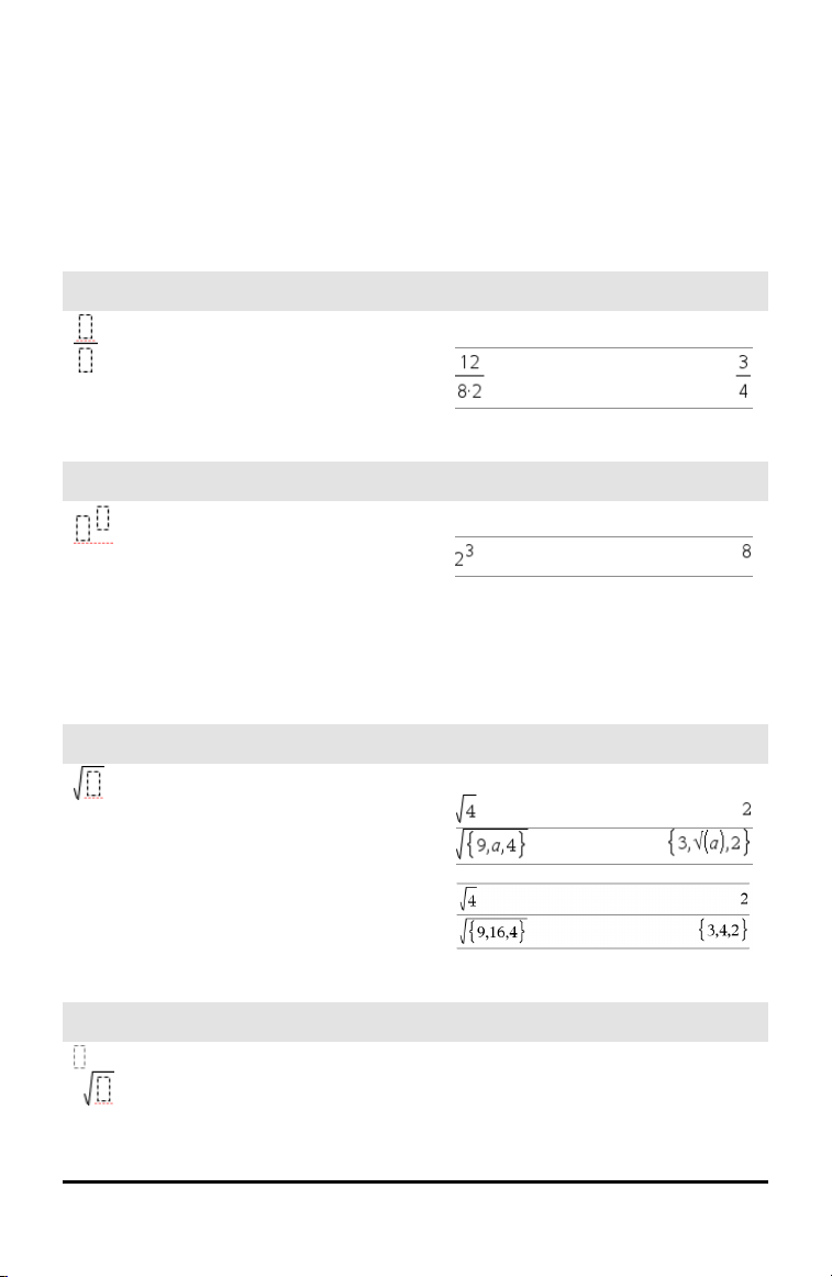
Fraction template

Note: See also / (divide), page 212.

Exponent template

Note: Type the first value, press l, and

then type the exponent. To return the cursor to the baseline, press right arrow (¢).

Note: See also ^ (power), page 213.

Square root template

Note: See also √() (square root), page

223.

/p keys

Example:

l key

Example:

/q keys

Example:

Nth root template

Note: See also root(), page 154.

/l keys

Example:

Expression T emplates 1

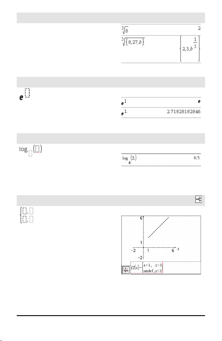
Nth root template

/l keys

e exponent template

Natural exponential e raised to a power

Note: See also e^(), page 57.

Log template

Calculates log to a specified base. For a default of base 10, omit the base.

Note: See also log(), page 107.

Piecewise template (2-piece)

Lets you create expressions and conditions for a two-piece piecewise function. To add a piece, click in the template and repeat the template.

Note: See also piecewise(), page 133.

u keys

Example:

/s key

Example:

Catalog >

Example:

2 Expression Templates

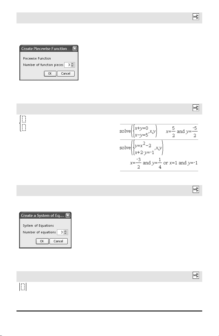
Piecewise template (N-piece)

Lets you create expressions and conditions for an N-piece piecewise function. Prompts for N.

Note: See also piecewise(), page 133.

Catalog >

Example:

See the example for Piecewisetemplate (2piece).

System of 2 equations template

Creates a system of two equations. To add a row to an existing system, click in the template and repeat the template.

Note: See also system(), page 182.

System of N equations template

Lets you create a system of N equations. Prompts for N.

Note: See also system(), page 182.

Absolute value template

Note: See also abs(), page 8.

Catalog >

Example:

Catalog >

Example:

See the example for Systemof equations template (2-equation).

Catalog >

Example:

Expression T emplates 3

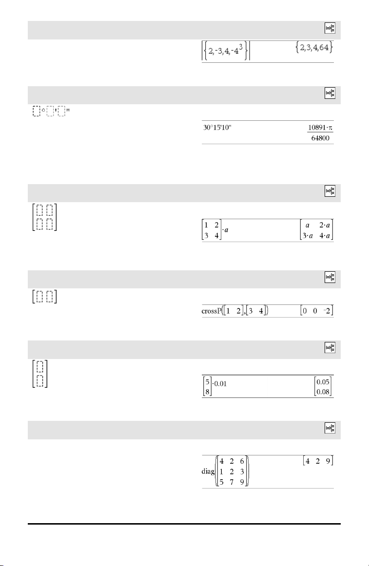
Absolute value template

Catalog >

dd°mm’ss.ss’’ template

Lets you enter angles in dd°mm’ss.ss’’ format, where dd is the number of decimal degrees, mm is the number of minutes, and

ss.ss is the number of seconds.

Matrix template (2 x 2)

Creates a 2 x 2 matrix.

Matrix template (1 x 2)

Matrix template (2 x 1)

Catalog >

Example:

Catalog >

Example:

Catalog >

Example:

Catalog >

Example:

Matrix template (m x n)

The template appears after you are prompted to specify the number of rows and columns.

4 Expression Templates

Catalog >

Example:

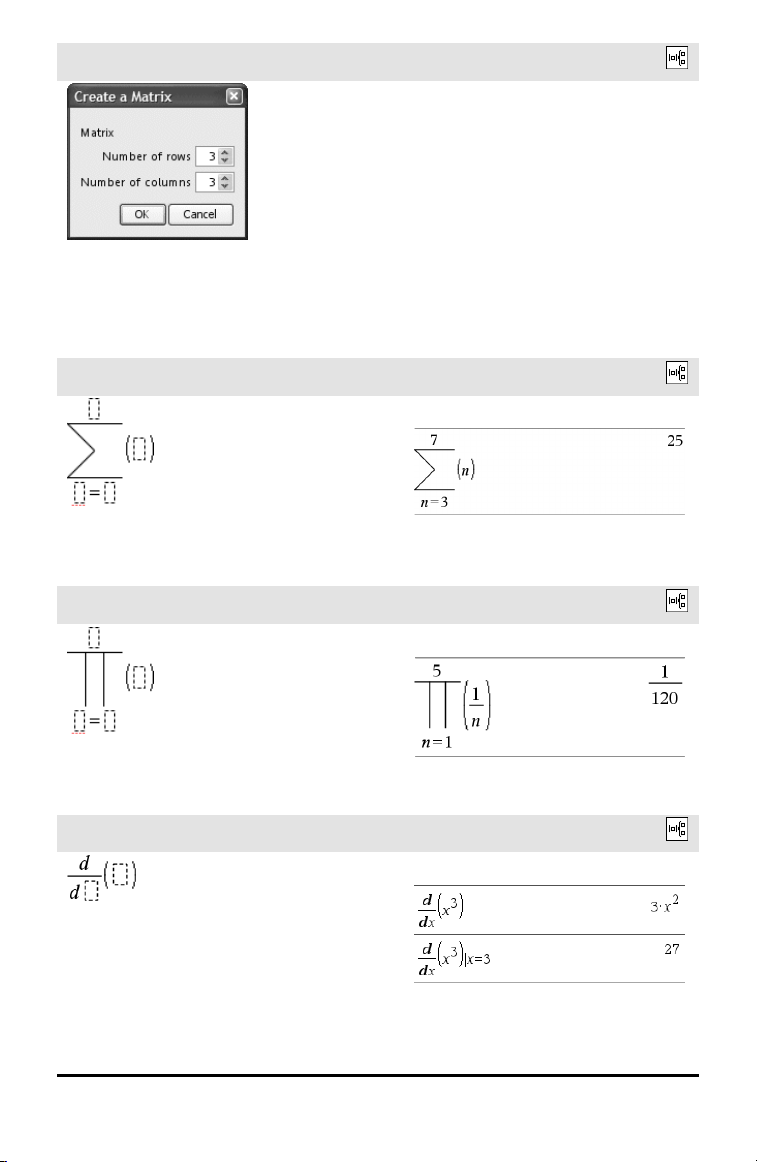
Matrix template (m x n)

Note: If you create a matrix with a large

number of rows and columns, it may take a few moments to appear.

Catalog >

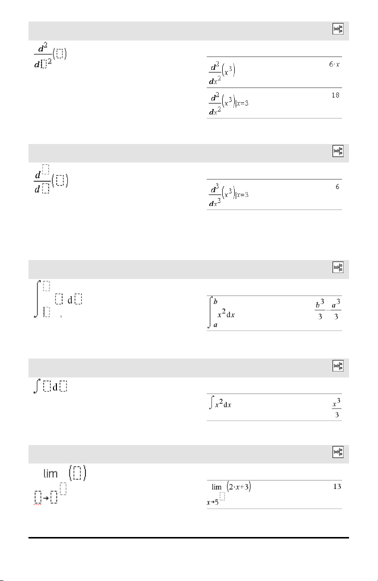
Sum template (Σ)

Note: See also Σ() (s umSeq), page 224.

Product template (Π)

Note: See also Π() (prodSeq), page 223.

First derivative template

The first derivative template can also be used to calculate first derivative at a point.

Note: See also d() (derivative), page 221.

Catalog >

Example:

Catalog >

Example:

Catalog >

Example:

Expression T emplates 5

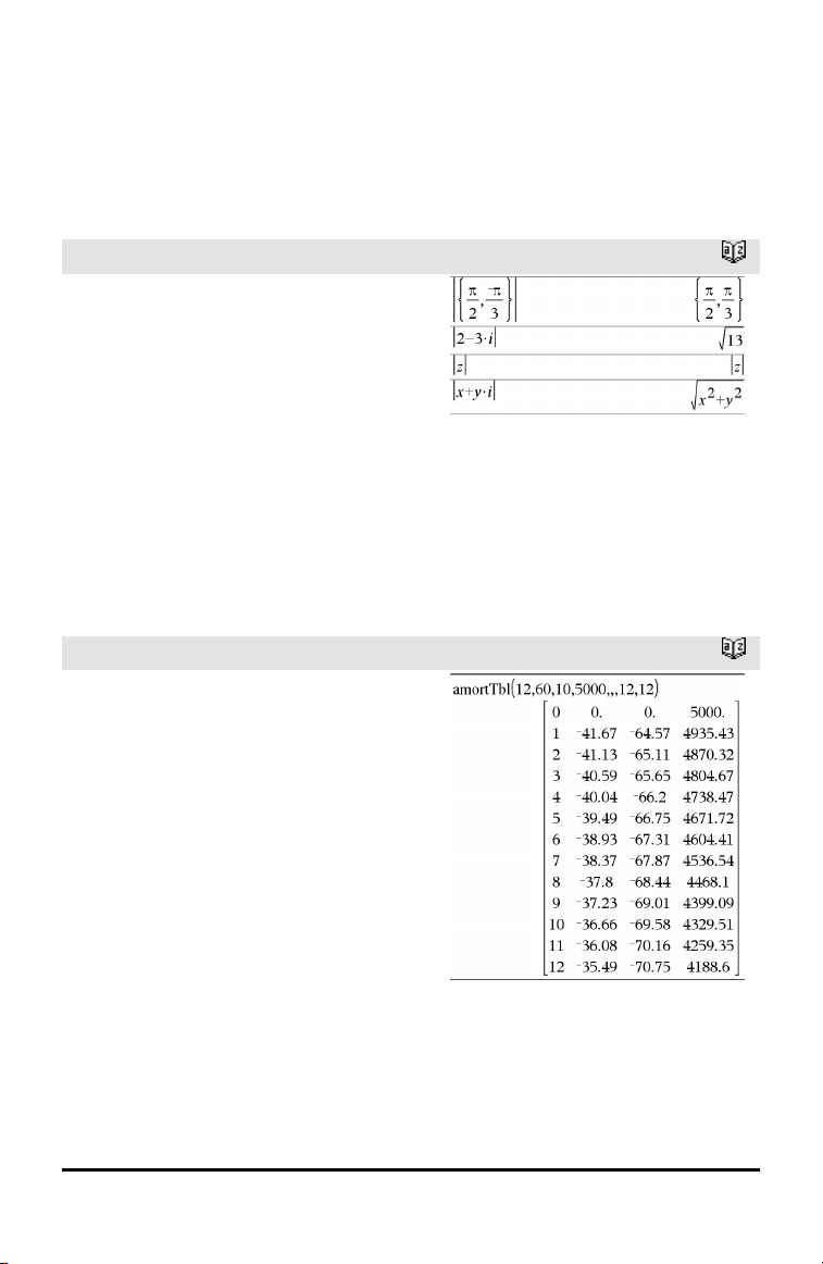
Second derivative template

The second derivative template can also be used to calculate second derivative at a point.

Note: See also d() (derivative), page 221.

Catalog >

Example:

Nth derivative template

The nth derivative template can be used to calculate the nth derivative.

Note: See also d() (derivative), page 221.

Definite integral template

Note: See also∫() integral(), page 221.

Indefinite integral template

Note: See also ∫() integral(), page 221.

Catalog >

Example:

Catalog >

Example:

Catalog >

Example:

Limit template

6 Expression Templates

Catalog >

Example:

Limit template

Use − or (−) for left hand limit. Use + for right hand limit.

Note: See also limit(), page 6.

Catalog >

Expression T emplates 7

Alphabetical Listing

Items whose names are not alphabetic (such as +, !, and >) are listed at the end of this section, page 210. Unless otherwise specified, all examples in this section were performed in the default reset mode, and all variables are assumed to be undefined.

abs()

abs(Expr1) ⇒ expression

abs(List1) ⇒ list abs(Matrix1) ⇒ matrix

Returns the absolute value of the argument.

Note: See also Absolute value template,

page 3.

If the argument is a complex number, returns the number’s modulus.

Note: All undefined variables are treated as

real variables.

amortTbl()

amortTbl(NPmt,N,I,PV, [Pmt], [FV], [PpY], [CpY], [PmtAt], [roundValue]) ⇒

matrix

Amortization function that returns a matrix as an amortization table for a set of TVM arguments.

NPmt is the number of payments to be

included in the table. The table starts with the first payment.

N, I, PV, Pmt, FV, PpY, CpY, and PmtAt

are described in the table of TVM arguments, page 195.

• If you omit Pmt, it defaults to

Pmt=tvmPmt

(N,I,PV,FV,PpY,CpY,PmtAt).

• If you omit FV, it defaults to FV=0.

• The defaults for PpY, CpY, and PmtAt are the same as for the TVM functions.

Catalog >

8 Alphabetical Listing

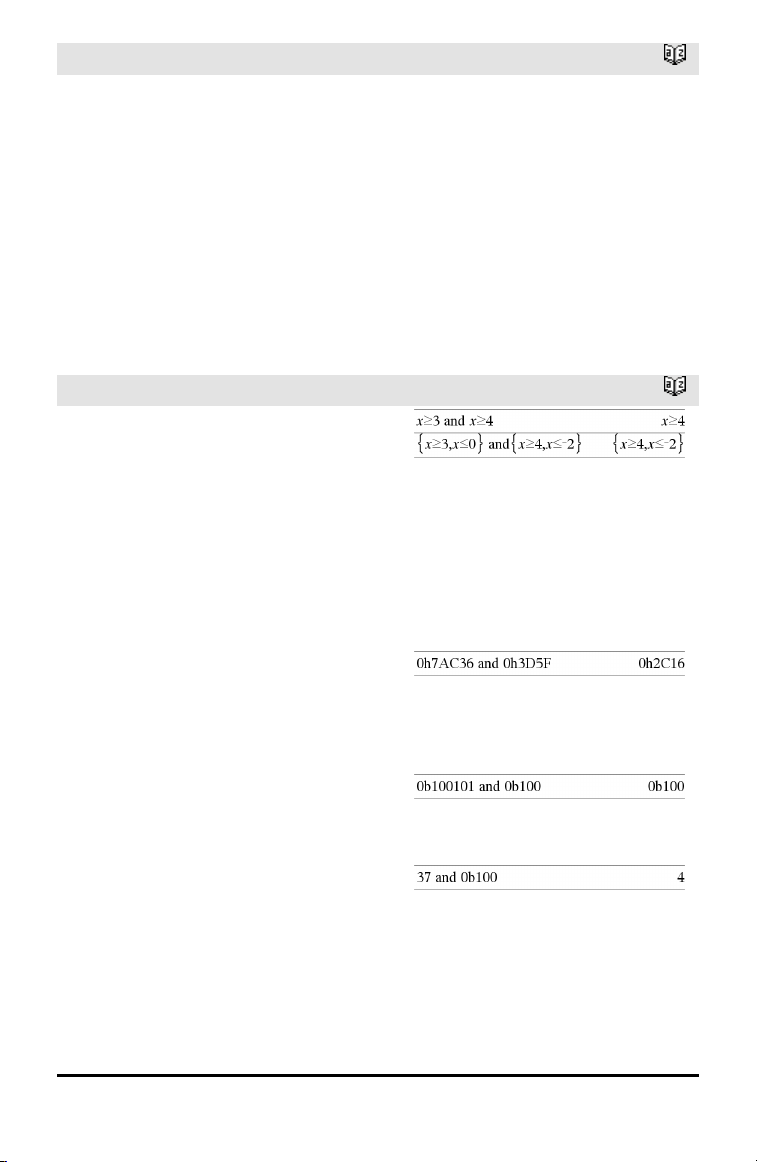
amortTbl()

roundValue specifies the number of

decimal places for rounding. Default=2.

The columns in the result matrix are in this order: Payment number, amount paid to interest, amount paid to principal, and balance.

The balance displayed in row n is the balance after payment n.

You can use the output matrix as input for the other amortization functions ΣInt() and

ΣPrn(), page 225, and bal(), page 17.

Catalog >

and

BooleanExpr1 and BooleanExpr2 ⇒ Boolean expression

BooleanList1 and BooleanList2 ⇒ Boolean list

BooleanMatrix1 and BooleanMatrix2 ⇒ Boolean matrix

Returns true or false or a simplified form of the original entry.

Integer1 andInteger2 ⇒ integer

Compares two real integers bit-by-bit using an and operation. Internally, both integers are converted to signed, 64-bit binary numbers. When corresponding bits are compared, the result is 1 if both bits are 1; otherwise, the result is 0. The returned value represents the bit results, and is displayed according to the Base mode.

You can enter the integers in any number base. For a binary or hexadecimal entry, you must use the 0b or 0h prefix, respectively. Without a prefix, integers are treated as decimal (base10).

Catalog >

In Hex basemode:

Important: Zero, not the letter O.

In Binbasemode:

In Dec base mode:

Note: A binary entry canhave upto 64 digits

(not countingthe0b prefix). A hexadecimal entry canhave up to 16 digits.

Alphabetical Listing 9

angle()

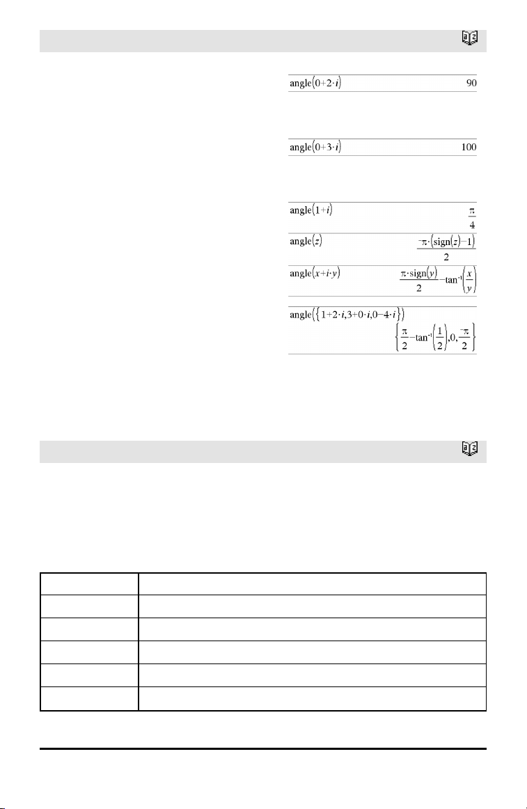
angle(Expr1) ⇒ expression

Returns the angle of the argument, interpreting the argument as a complex number.

Note: All undefined variables are treated as

real variables.

angle(List1) ⇒ list angle(Matrix1) ⇒ matrix

Returns a list or matrix of angles of the elements in List1 or Matrix1, interpreting each element as a complex number that represents a two-dimensional rectangular coordinate point.

Catalog >

In Degree angle mode:

In Gradianangle mode:

In Radian angle mode:

ANOVA

Catalog >

ANOVA List1,List2[,List3,...,List20][,Flag]

Performs a one-way analysis of variance for comparing the means of two to 20 populations. A summary of results is stored in the stat.results variable. (page 177)

Flag=0 for Data, Flag=1 for Stats

Output variable Description

stat.F Valueof the F statistic

stat.PVal Smallest level of significance at which thenull hypothesis can be rejected

stat.df Degrees of freedom of the groups

stat.SS Sum of squaresof thegroups

stat.MS Mean squares for the groups

10 A lphabetical Listing

Output variable Description

stat.dfError Degrees of freedom of the errors

stat.SSError Sum of squaresof theerrors

stat.MSError Mean square for the errors

stat.sp Pooled standard deviation

stat.xbarlist Mean of the inputof the lists

stat.CLowerList 95%confidence intervals for the mean of each inputlist

stat.CUpperList 95%confidenceintervals for the mean of each inputlist

ANOVA2way

Catalog >

ANOVA2way List1,List2[,List3,…,List10]

[,levRow]

Computes a two-way analysis of variance for comparing the means of two to 10 populations. A summary of results is stored in the stat.results variable. (See page 177.)

LevRow=0 for Block

LevRow=2,3,...,Len-1, for Two Factor,

where Len=length(List1)=length(List2) = … = length(List10) and Len/LevRow Î {2,3,…}

Outputs: Block Design

Output variable Description

stat.F Fstatistic of the columnfactor

stat.PVal Smallest level of significance at which thenull hypothesis can be rejected

stat.df Degrees of freedom of the columnfactor

stat.SS Sum of squaresof thecolumn factor

stat.MS Mean squares for columnfactor

stat.FBlock F statisticfor factor

stat.PValBlock Leastprobability atwhichthe nullhypothesiscanbe rejected

stat.dfBlock Degrees of freedom for factor

stat.SSBlock Sumof squares for factor

Alphabetical Listing 11

Output variable Description

stat.MSBlock Mean squares for factor

stat.dfError Degrees of freedom of the errors

stat.SSError Sum of squaresof theerrors

stat.MSError Mean squares for the errors

stat.s Standard deviation of the error

COLUMN FACTOR Outputs

Output variable Description

stat.Fcol F statistico f the columnfactor

stat.PValCol Probability valueof the columnfactor

stat.dfCol Degrees of freedom of the columnfactor

stat.SSCol Sum of squaresof thecolumn factor

stat.MSCol Mean squares for columnfactor

ROW FACTOR Outputs

Output variable Description

stat.FRow F statisticof the row factor

stat.PValRow Probability valueof the row factor

stat.dfRow Degrees of freedom of the ro w factor

stat.SSRow Sum of squaresof the row factor

stat.MSRow Mean squares for row factor

INTERACTION Outputs

Output variable Description

stat.FInteract F statisticof the interaction

stat.PValInteract Probability valueof the interaction

stat.dfInteract Degrees of freedom of the interaction

stat.SSInteract Sum of squaresof theinteraction

stat.MSInteract Mean squares for interaction

ERROR Outputs

12 A lphabetical Listing

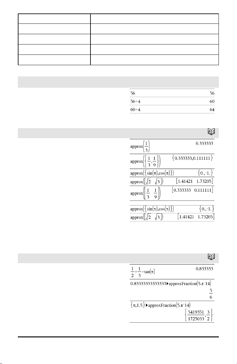
Output variable Description

stat.dfError Degrees of freedom of the errors

stat.SSError Sum of squaresof theerrors

stat.MSError Mean squares for the errors

s Standard deviation of the error

Ans

Ans ⇒ value

Returns the result of the most recently evaluated expression.

approx()

approx(Expr1) ⇒ expression

Returns the evaluation of the argument as an expression containing decimal values, when possible, regardless of the current

Auto or Approximate mode.

This is equivalent to entering the argument and pressing /·.

approx(List1) ⇒ list approx(Matrix1) ⇒ matrix

Returns a list or matrix where each element has been evaluated to a decimal value, when possible.

►approxFraction()

Expr►approxFraction([Tol]) ⇒ expression

/v keys

Catalog >

List►approxFraction([Tol]) ⇒ list

Matrix►approxFraction([Tol]) ⇒ matrix

Returns the input as a fraction, using a tolerance of Tol. If Tol is omitted, a tolerance of 5.E-14 is used.

Alphabetical Listing 13

►approxFraction()

Note: You can insert this function from the

computer keyboard by typing

@>approxFraction(...).

Catalog >

approxRational()

approxRational(Expr[, Tol]) ⇒ expression

approxRational(List[, Tol]) ⇒ list

approxRational(Matrix[, Tol]) ⇒ matrix

Returns the argument as a fraction using a tolerance of Tol. If Tol is omitted, a tolerance of 5.E-14 is used.

arccos()

arccosh()

arccot()

arccoth()

Catalog >

See cos⁻¹(), page 31.

See cosh⁻¹(), page 32.

See cot⁻¹(), page 33.

See coth⁻¹(), page 34.

arccsc()

arccsch()

14 A lphabetical Listing

See csc⁻¹(), page 37.

See csch⁻¹(), page 37.

arcLen()

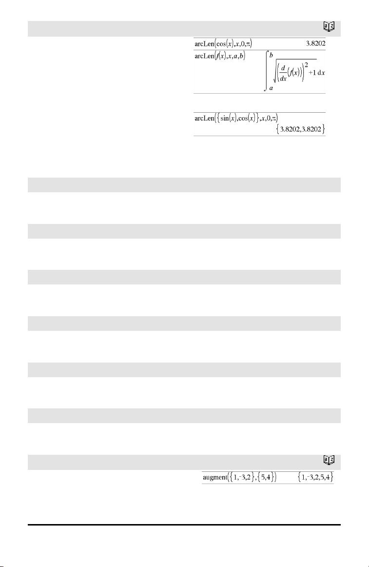
arcLen(Expr1,Var,Start,End) ⇒

expression

Returns the arc length of Expr1 from

Start to End with respect to variable Var.

Arc length is calculated as an integral assuming a function mode definition.

arcLen(List1,Var,Start,End) ⇒ list

Returns a list of the arc lengths of each element of List1 from Start to End with respect to Var.

Catalog >

arcsec()

arcsech()

arcsin()

arcsinh()

arctan()

arctanh()

augment()

augment(List1, List2) ⇒ list

See sec⁻¹(), page 158.

See sech⁻¹(), page 158.

See sin⁻¹(), page 168.

See sinh⁻¹(), page 169.

See tan⁻¹(), page 183.

See tanh⁻¹(), page 185.

Catalog >

Alphabetical Listing 15

augment()

Returns a new list that is List2 appended to the end of List1.

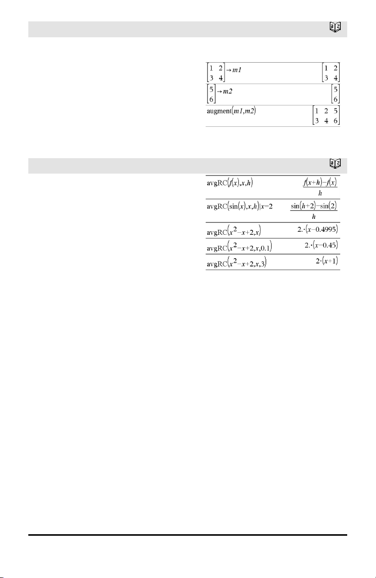
augment(Matrix1, Matrix2) ⇒ matrix

Returns a new matrix that is Matrix2 appended to Matrix1. When the “,” character is used, the matrices must have equal row dimensions, and Matrix2 is appended to Matrix1 as new columns. Does not alter Matrix1 or Matrix2.

Catalog >

avgRC()

avgRC(Expr1, Var [=Value] [, Step]) ⇒

expression

avgRC(Expr1, Var [=Value] [, List1]) ⇒

list

avgRC(List1, Var [=Value] [, Step]) ⇒

list

avgRC(Matrix1, Var [=Value] [, Step]) ⇒

matrix

Returns the forward-difference quotient (average rate of change).

Expr1 can be a user-defined function name

(see Func).

When Value is specified, it overrides any prior variable assignment or any current “|” substitution for the variable.

Step is the step value. If Step is omitted, it

defaults to 0.001.

Note that the similar function centralDiff() uses the central-difference quotient.

Catalog >

16 A lphabetical Listing

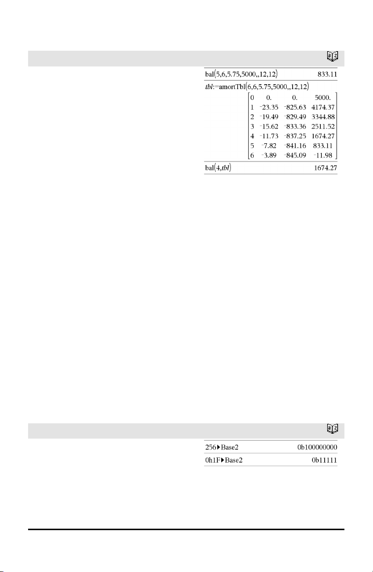
bal()

bal(NPmt,N,I,PV ,[Pmt], [FV], [PpY], [CpY], [PmtAt], [roundValue]) ⇒ value

bal(NPmt,amortTable) ⇒ value

Amortization function that calculates schedule balance after a specified payment.

N, I, PV, Pmt, FV, PpY, CpY, and PmtAt

are described in the table of TVM arguments, page 195.

NPmt specifies the payment number after

which you want the data calculated.

N, I, PV, Pmt, FV, PpY, CpY, and PmtAt

are described in the table of TVM arguments, page 195.

• If you omit Pmt, it defaults to

Pmt=tvmPmt

(N,I,PV,FV,PpY,CpY,PmtAt).

• If you omit FV, it defaults to FV=0.

• The defaults for PpY, CpY, and PmtAt are the same as for the TVM functions.

roundValue specifies the number of

decimal places for rounding. Default=2.

bal(NPmt,amortTable) calculates the

balance after payment number NPmt, based on amortization table amortTable. The amortTable argument must be a matrix in the form described under

amortTbl(), page 8. Note: See also ΣInt() and ΣPrn(), page 225.

Catalog >

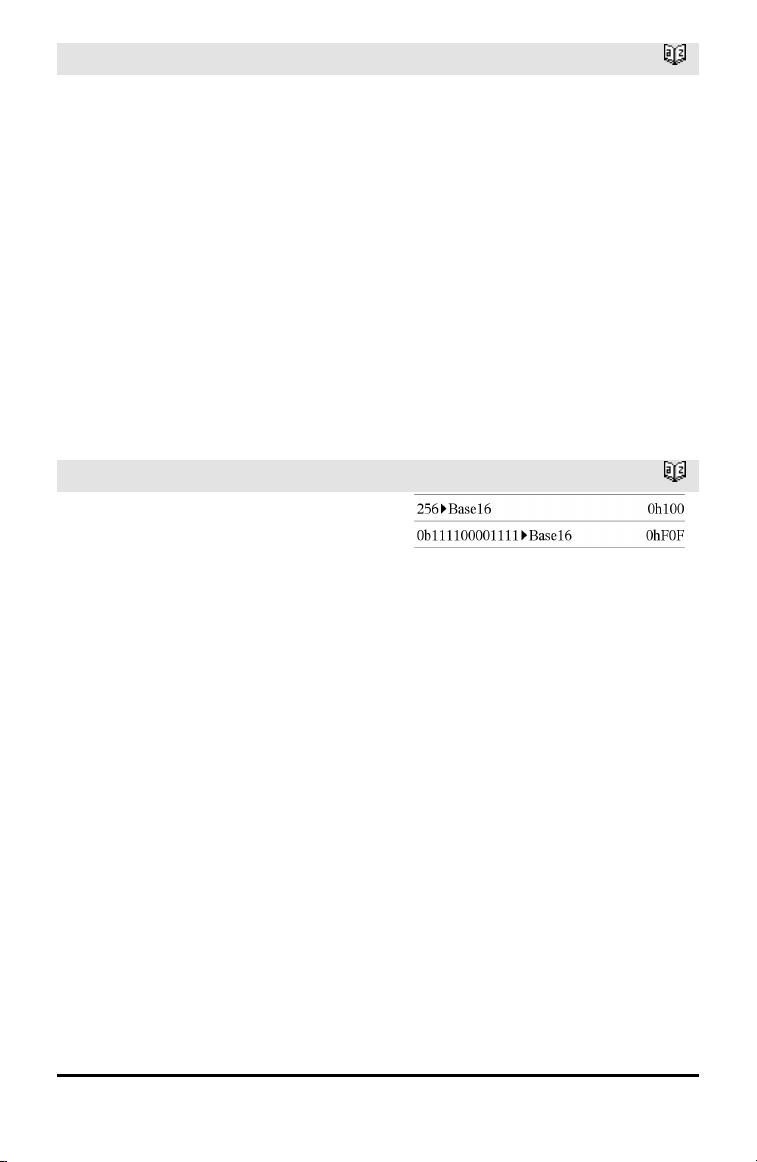
►Base2

Integer1 ►Base2 ⇒ integer

Note: You can insert this operator from the

computer keyboard by typing @>Base2.

Catalog >

Alphabetical Listing 17

►Base2

Converts Integer1 to a binary number. Binary or hexadecimal numbers always have a 0b or 0h prefix, respectively. Use a zero, not the letter O, followed by b or h.

0b binaryNumber 0h hexadecimalNumber

A binary number can have up to 64 digits. A hexadecimal number can have up to 16.

Without a prefix, Integer1 is treated as decimal (base10). The result is displayed in binary, regardless of the Base mode.

Negative numbers are displayed in “two's complement” form. For example,

⁻1is displayed as

0hFFFFFFFFFFFFFFFFin Hex base mode 0b111...111 (641’s)in Binary base mode

⁻2

is displayed as 0h8000000000000000in Hex base mode 0b100...000 (63 zeros)in Binary base mode

If you enter a decimal integer that is outside the range of a signed, 64-bit binary form, a symmetric modulo operation is used to bring the value into the appropriate range. Consider the following examples of values outside the range.

263becomes ⁻263and is displayed as 0h8000000000000000in Hex base mode 0b100...000 (63 zeros)in Binary base mode

264becomes 0 and is displayed as 0h0in Hex base mode 0b0in Binary base mode

⁻263− 1 becomes 263− 1 and is displayed

as 0h7FFFFFFFFFFFFFFFin Hex base mode 0b111...111 (641’s)in Binary base mode

Catalog >

►Base10

Integer1 ►Base10 ⇒ integer

18 A lphabetical Listing

Catalog >

►Base10

Note: You can insert this operator from the

computer keyboard by typing @>Base10.

Converts Integer1 to a decimal (base10) number. A binary or hexadecimal entry must always have a 0b or 0h prefix, respectively.

0b binaryNumber 0h hexadecimalNumber

Zero, not the letter O, followed by b or h.

A binary number can have up to 64 digits. A hexadecimal number can have up to 16.

Without a prefix, Integer1 is treated as decimal. The result is displayed in decimal, regardless of the Base mode.

Catalog >

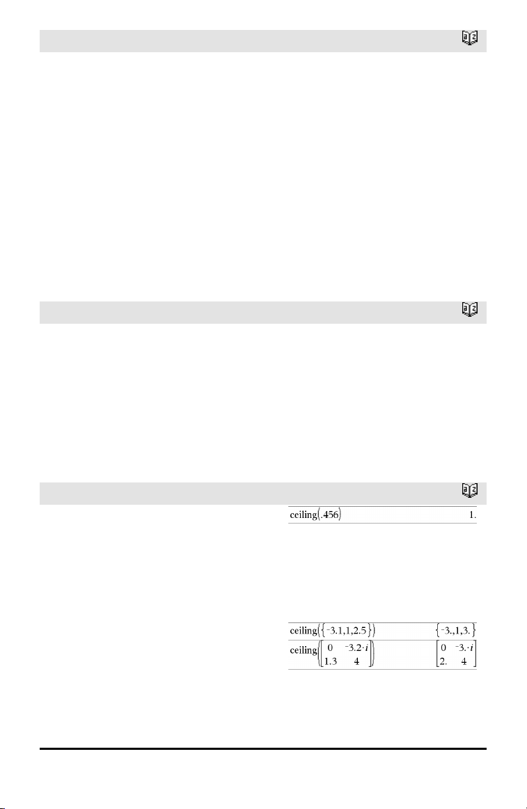
►Base16

Integer1 ►Base16 ⇒ integer

Note: You can insert this operator from the

computer keyboard by typing @>Base16.

Converts Integer1 to a hexadecimal number. Binary or hexadecimal numbers always have a 0b or 0h prefix, respectively.

0b binaryNumber 0h hexadecimalNumber

Zero, not the letter O, followed by b or h.

A binary number can have up to 64 digits. A hexadecimal number can have up to 16.

Without a prefix, Integer1 is treated as decimal (base10). The result is displayed in hexadecimal, regardless of the Base mode.

If you enter a decimal integer that is too large for a signed, 64-bit binary form, a symmetric modulo operation is used to bring the value into the appropriate range. For more information, see ►Base2, page

17.

Catalog >

Alphabetical Listing 19

binomCdf()

binomCdf(n,p) ⇒ list

binomCdf(n,p,lowBound,upBound) ⇒

number if lowBound and upBound are

numbers, list if lowBound and upBound are lists

binomCdf(n,p,upBound)for P(0≤X≤upBound)

⇒ number if upBound is a number, list if upBound is a list

Computes a cumulative probability for the discrete binomial distribution with n number of trials and probability p of success on each trial.

For P(X ≤ upBound), set lowBound=0

Catalog >

binomPdf()

binomPdf(n,p) ⇒ list

binomPdf(n,p,XVal) ⇒ number if XVal is a

number, list if XVal is a list

Computes a probability for the discrete binomial distribution with n number of trials and probability p of success on each trial.

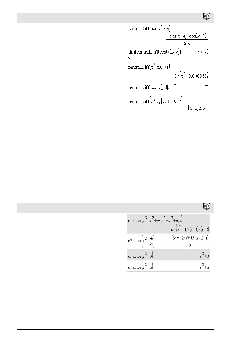
ceiling(Expr1) ⇒ integer

Returns the nearest integer that is ≥ the argument.

The argument can be a real or a complex number.

Note: See also floor().

ceiling(List1) ⇒ list ceiling(Matrix1) ⇒ matrix

Returns a list or matrix of the ceiling of each element.

Catalog >

20 A lphabetical Listing

centralDiff()

centralDiff(Expr1,Var [=Value][,Step]) ⇒

expression

centralDiff(Expr1,Var [,Step])|Var=Value

⇒ expression

centralDiff(Expr1,Var [=Value][,List]) ⇒

list

centralDiff(List1,Var [=Value][,Step]) ⇒

list

centralDiff(Matrix1,Var [=Value][,Step])

⇒ matrix

Returns the numerical derivative using the central difference quotient formula.

When Value is specified, it overrides any prior variable assignment or any current “|” substitution for the variable.

Step is the step value. If Step is omitted, it

defaults to 0.001.

When using List1 or Matrix1, the operation gets mapped across the values in the list or across the matrix elements.

Note: See also avgRC() and d().

Catalog >

cFactor()

cFactor(Expr1[,Var]) ⇒ expression cFactor(List1[,Var]) ⇒ list cFactor(Matrix1[,Var]) ⇒ matrix

cFactor(Expr1) returns Expr1 factored with

respect to all of its variables over a common denominator.

Expr1 is factored as much as possible

toward linear rational factors even if this introduces new non-real numbers. This alternative is appropriate if you want factorization with respect to more than one variable.

Catalog >

Alphabetical Listing 21

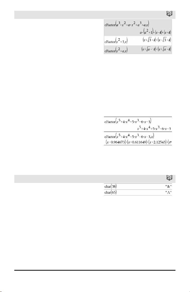
cFactor()

cFactor(Expr1,Var) returns Expr1 factored

with respect to variable Var.

Expr1 is factored as much as possible

toward factors that are linear in Var, with perhaps non-real constants, even if it introduces irrational constants or subexpressions that are irrational in other variables.

The factors and their terms are sorted with

Var as the main variable. Similar powers of Var are collected in each factor. Include Var if factorization is needed with respect

to only that variable and you are willing to accept irrational expressions in any other variables to increase factorization with respect to Var. There might be some incidental factoring with respect to other variables.

For the Auto setting of the Auto or

Approximate mode, including Var also

permits approximation with floating-point coefficients where irrational coefficients cannot be explicitly expressed concisely in terms of the built-in functions. Even when there is only one variable, including Var might yield more complete factorization.

Note: See also factor().

Catalog >

To see the entire result, press £ and then use¡and¢ to move thecursor.

char()

char(Integer) ⇒ character

Returns a character string containing the character numbered Integer from the handheld character set. The valid range for

Integer is 0–65535.

22 A lphabetical Listing

Catalog >

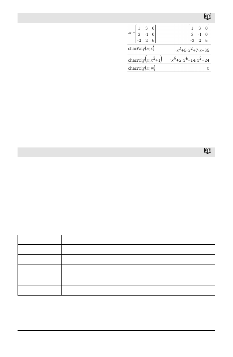
charPoly()

charPoly(squareMatrix,Var) ⇒

polynomial expression

charPoly(squareMatrix,Expr) ⇒

polynomial expression

charPoly(squareMatrix1,Matrix2) ⇒

polynomial expression

Returns the characteristic polynomial of

squareMatrix. The characteristic

polynomial of n×n matrix A, denoted by p (λ), is the polynomial defined by

(λ) = det(λ•I−A)

where I denotes the n×n identity matrix.

squareMatrix1 and squareMatrix2 must

have the equal dimensions.

Catalog >

2way

2way obsMatrix

Catalog >

chi22way obsMatrix

Computes a χ2test for association on the two-way table of counts in the observed matrix obsMatrix. A summary of results is stored in the stat.results variable. (page

177)

For information on the effect of empty elements in a matrix, see “Empty (Void) Elements,” page 236.

Output variable Description

stat.χ

stat.PVal Smallest level of significance at which thenull hypothesis can be rejected

stat.df Degrees of freedom for the chi square statistics

stat.ExpMat Matrix of expectedelemental counttable, assuming nullhypothesis

stat.CompMat Matrix of elementalchi square statisticcontributions

Chi square stat: sum (observed - expected)2/expected

Alphabetical Listing 23

Cdf()

Cdf(lowBound,upBound,df) ⇒ number if

lowBound and upBound are numbers, list if lowBound and upBound are lists

chi2Cdf(lowBound,upBound,df) ⇒ number

if lowBound and upBound are numbers, list if lowBound and upBound are lists

Computes the χ2distribution probability between lowBound and upBound for the specified degrees of freedom df.

For P(X ≤ upBound), set lowBound = 0.

For information on the effect of empty elements in a list, see “Empty (Void) Elements,” page 236.

Catalog >

GOF

GOF obsList,expList,df

Catalog >

chi2GOF obsList,expList,df

Performs a test to confirm that sample data is from a population that conforms to a specified distribution. obsList is a list of counts and must contain integers. A summary of results is stored in the

stat.results variable. (See page 177.)

For information on the effect of empty elements in a list, see “Empty (Void) Elements,” page 236.

Output variable Description

stat.χ

stat.PVal Smallest level of significance at which thenull hypothesis can be rejected

stat.df Degrees of freedom for the chi square statistics

stat.CompList Elemental chisquare statistic contributions

Pdf()

Pdf(XVal,df) ⇒ number if XVal is a

Chi square stat: sum((observed - expected)2/expected

Catalog >

number, list if XVal is a list

24 A lphabetical Listing

Pdf()

chi2Pdf(XVal,df) ⇒ number if XVal is a

number, list if XVal is a list

Computes the probability density function (pdf) for the χ2distribution at a specified

XVal value for the specified degrees of

freedom df.

For information on the effect of empty elements in a list, see “Empty (Void) Elements,” page 236.

Catalog >

ClearAZ

Clears all single-character variables in the current problem space.

If one or more of the variables are locked, this command displays an error message and deletes only the unlocked variables. See

unLock, page 197.

ClrErr

Clears the error status and sets system variable errCode to zero.

The Else clause of the Try...Else...EndTry block should use ClrErr or PassErr. If the error is to be processed or ignored, use

ClrErr. If what to do with the error is not

known, use PassErr to send it to the next error handler. If there are no more pending

Try...Else...EndTry error handlers, the error

dialog box will be displayed as normal.

Note: See also PassErr, page 132, and Try,

page 191.

Note for entering the example: For

instructions on entering multi-line program and function definitions, refer to the Calculator section of your product guidebook.

Catalog >

For an example of ClrErr, See Example 2 under the Try command, page 191.

Alphabetical Listing 25

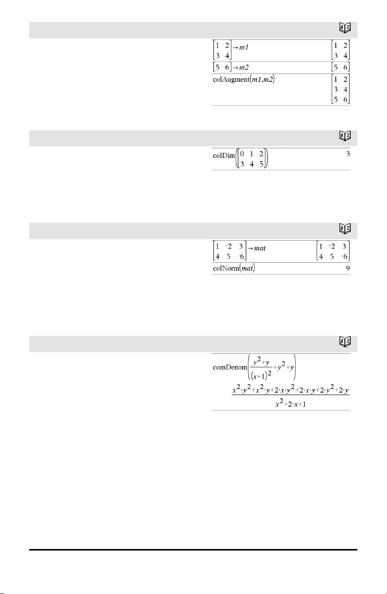
colAugment()

colAugment(Matrix1, Matrix2) ⇒ matrix

Returns a new matrix that is Matrix2 appended to Matrix1. The matrices must have equal column dimensions, and

Matrix2 is appended to Matrix1 as new

rows. Does not alter Matrix1 or Matrix2.

Catalog >

colDim()

colDim(Matrix) ⇒ expression

Returns the number of columns contained in Matrix.

Note: See also rowDim().

colNorm()

colNorm(Matrix) ⇒ expression

Returns the maximum of the sums of the absolute values of the elements in the columns in Matrix.

Note: Undefined matrix elements are not

allowed. See also rowNorm().

comDenom()

comDenom(Expr1[,Var]) ⇒ expression comDenom(List1[,Var]) ⇒ list comDenom(Matrix1[,Var]) ⇒ matrix

comDenom(Expr1) returns a reduced ratio

of a fully expanded numerator over a fully expanded denominator.

Catalog >

26 A lphabetical Listing

comDenom()

comDenom(Expr1,Var) returns a reduced

ratio of numerator and denominator expanded with respect to Var. The terms and their factors are sorted with Var as the main variable. Similar powers of Var are collected. There might be some incidental factoring of the collected coefficients. Compared to omitting Var, this often saves time, memory, and screen space, while making the expression more comprehensible. It also makes subsequent operations on the result faster and less likely to exhaust memory.

If Var does not occur in Expr1, comDenom

(Expr1,Var) returns a reduced ratio of an

unexpanded numerator over an unexpanded denominator. Such results usually save even more time, memory, and screen space. Such partially factored results also make subsequent operations on the result much faster and much less likely to exhaust memory.

Even when there is no denominator, the

comden function is often a fast way to

achieve partial factorization if factor() is too slow or if it exhausts memory.

Hint: Enter this comden() function definition

and routinely try it as an alternative to

comDenom() and factor().

Catalog >

completeSquare ()

completeSquare(ExprOrEqn, Var) ⇒

expression or equation

completeSquare(ExprOrEqn, Var^Power)

⇒ expression or equation

completeSquare(ExprOrEqn, Var1, Var2

[,...]) ⇒ expression or equation

completeSquare(ExprOrEqn, {Var1, Var2

[,...]}) ⇒ expression or equation

Converts a quadratic polynomial expression of the form a•x2+b•x+c into the form a•(x-h)

Catalog >

Alphabetical Listing 27

completeSquare ()

- or -

Converts a quadratic equation of the form a•x2+b•x+c=d into the form a•(x-h)2=k

The first argument must be a quadratic expression or equation in standard form with respect to the second argument.

The Second argument must be a single univariate term or a single univariate term raised to a rational power, for example x,y2,orz

The third and fourth syntax attempt to complete the square with respect to variables Var1, Var2 [,… ]).

(1/3)

Catalog >

conj()

conj(Expr1) ⇒ expression

conj(List1) ⇒ list

conj(Matrix1) ⇒ matrix

Returns the complex conjugate of the argument.

Note: All undefined variables are treated as

real variables.

constructMat()

constructMat (Expr,Var1,Var2,numRows,numCols) ⇒

matrix

Returns a matrix based on the arguments.

Expr is an expression in variables Var1 and Var2. Elements in the resulting matrix are

formed by evaluating Expr for each incremented value of Var1 and Var2.

Var1 is automatically incremented from 1

through numRows. Within each row, Var2 is incremented from 1 through numCols.

Catalog >

28 A lphabetical Listing

CopyVar

CopyVar Var1, Var2

CopyVar Var1., Var2.

CopyVar Var1, Var2 copies the value of

variable Var1 to variable Var2, creating

Var2 if necessary. Variable Var1 must have

a value.

If Var1 is the name of an existing userdefined function, copies the definition of that function to function Var2. Function

Var1 must be defined.

Var1 must meet the variable-naming

requirements or must be an indirection expression that simplifies to a variable name meeting the requirements.

CopyVar Var1., Var2. copies all members

of the Var1. variable group to the Var2. group, creating Var2. if necessary.

Var1. must be the name of an existing

variable group, such as the statistics stat.nn results, or variables created using the

LibShortcut() function. If Var2. already

exists, this command replaces all members that are common to both groups and adds the members that do not already exist. If one or more members of Var2. are locked, all members of Var2. are left unchanged.

Catalog >

corrMat()

corrMat(List1,List2[,…[,List20]])

Computes the correlation matrix for the augmented matrix [List1, List2, ..., List20].

►cos

Expr ►cos

Note: You can insert this operator from the

computer keyboard by typing @>cos.

Represents Expr in terms of cosine. This is a display conversion operator. It can be used only at the end of the entry line.

Catalog >

Alphabetical Listing 29

►cos

►cos reduces all powers of

sin(...) modulo 1−cos(...)^2 so that any remaining powers of cos(...) have exponents in the range (0, 2). Thus, the result will be free of sin(...) if and only if sin(...) occurs in the given expression only to even powers.

Note: This conversion operator is not

supported in Degree or Gradian Angle modes. Before using it, make sure that the Angle mode is set to Radians and that Expr does not contain explicit references to degree or gradian angles.

Catalog >

cos()

cos(Expr1) ⇒ expression

cos(List1) ⇒ list

cos(Expr1) returns the cosine of the

argument as an expression.

cos(List1) returns a list of the cosines of all

elements in List1.

Note: The argument is interpreted as a

degree, gradian or radian angle, according to the current angle mode setting. You can use °,G, orrto override the angle mode temporarily.

cos(squareMatrix1) ⇒ squareMatrix

Returns the matrix cosine of

squareMatrix1. This is not the same as

calculating the cosine of each element.

µ key

In Degree angle mode:

In Gradianangle mode:

In Radian angle mode:

30 A lphabetical Listing

cos()

When a scalar function f(A) operates on

squareMatrix1 (A), the result is calculated

by the algorithm: Compute the eigenvalues (λi) and

eigenvectors (Vi) of A.

squareMatrix1 must be diagonalizable.

Also, it cannot have symbolic variables that have not been assigned a value.

Form the matrices:

Then A = X B X⁻¹ and f(A) = X f(B) X⁻¹. For example, cos(A) = X cos(B) X⁻¹ where:

cos(B) =

All computations are performed using floating-point arithmetic.

µ key

cos⁻¹()

cos⁻¹(Expr1) ⇒ expression

cos⁻¹(List1) ⇒ list

cos⁻¹(Expr1) returns the angle whose

cosine is Expr1 as an expression.

cos⁻¹(List1) returns a list of the inverse

cosines of each element of List1.

Note: The result is returned as a degree,

gradian or radian angle, according to the current angle mode setting.

Note: You can insert this function from the

keyboard by typing arccos(...).

µ key

In Degree angle mode:

In Gradianangle mode:

In Radian angle mode:

Alphabetical Listing 31

cos⁻¹()

cos⁻¹(squareMatrix1) ⇒ squareMatrix

Returns the matrix inverse cosine of

squareMatrix1. This is not the same as

calculating the inverse cosine of each element. For information about the calculation method, refer to cos().

squareMatrix1 must be diagonalizable. The

result always contains floating-point numbers.

µ key

In Radian angle mode and Rectangular Complex Format:

To see the entire result, press £ and then use¡and¢ to move thecursor.

cosh()

cosh(Expr1) ⇒ expression

cosh(List1) ⇒ list

cosh(Expr1) returns the hyperbolic cosine

of the argument as an expression.

cosh(List1) returns a list of the hyperbolic

cosines of each element of List1.

cosh(squareMatrix1) ⇒ squareMatrix

Returns the matrix hyperbolic cosine of

squareMatrix1. This is not the same as

calculating the hyperbolic cosine of each element. For information about the calculation method, refer to cos().

squareMatrix1 must be diagonalizable. The

result always contains floating-point numbers.

cosh⁻¹()

cosh⁻¹(Expr1) ⇒ expression

cosh⁻¹(List1) ⇒ list

cosh⁻¹(Expr1) returns the inverse

hyperbolic cosine of the argument as an expression.

Catalog >

In Degree angle mode:

In Radian angle mode:

Catalog >

32 A lphabetical Listing

cosh⁻¹()

cosh⁻¹(List1) returns a list of the inverse

hyperbolic cosines of each element of

List1.

Note: You can insert this function from the

keyboard by typing arccosh(...).

cosh⁻¹(squareMatrix1) ⇒ squareMatrix

Returns the matrix inverse hyperbolic cosine of squareMatrix1. This is not the same as calculating the inverse hyperbolic cosine of each element. For information about the calculation method, refer to cos

().

squareMatrix1 must be diagonalizable. The

result always contains floating-point numbers.

Catalog >

In Radian angle mode and In Rectangular Complex Format:

To see the entire result, press £ and then use¡and¢ to move thecursor.

cot()

cot(Expr1) ⇒ expression

cot(List1) ⇒ list

Returns the cotangent of Expr1 or returns a list of the cotangents of all elements in

List1.

Note: The argument is interpreted as a

degree, gradian or radian angle, according to the current angle mode setting. You can use °,G, orrto override the angle mode temporarily.

cot⁻¹()

cot⁻¹(Expr1) ⇒ expression

cot⁻¹(List1) ⇒ list

Returns the angle whose cotangent is

Expr1 or returns a list containing the

inverse cotangents of each element of

List1.

µ key

In Degree angle mode:

In Gradianangle mode:

In Radian angle mode:

µ key

In Degree angle mode:

In Gradianangle mode:

Alphabetical Listing 33

cot⁻¹()

Note: The result is returned as a degree,

gradian or radian angle, according to the current angle mode setting.

Note: You can insert this function from the

keyboard by typing arccot(...).

µ key

In Radian angle mode:

coth()

coth(Expr1) ⇒ expression

coth(List1) ⇒ list

Returns the hyperbolic cotangent of Expr1 or returns a list of the hyperbolic cotangents of all elements of List1.

coth⁻¹()

coth⁻¹(Expr1) ⇒ expression

coth⁻¹(List1) ⇒ list

Returns the inverse hyperbolic cotangent of

Expr1 or returns a list containing the

inverse hyperbolic cotangents of each element of List1.

Note: You can insert this function from the

keyboard by typing arccoth(...).

count()

count(Value1orList1 [,Value2orList2

[,...]]) ⇒ value

Returns the accumulated count of all elements in the arguments that evaluate to numeric values.

Each argument can be an expression, value, list, or matrix. You can mix data types and use arguments of various dimensions.

For a list, matrix, or range of cells, each element is evaluated to determine if it should be included in the count.

Catalog >

In the last example, only 1/2 and 3+4*i are counted. Theremaining arguments, assumingx is undefined, do notevaluate to numericvalues.

34 A lphabetical Listing

count()

Within the Lists & Spreadsheet application, you can use a range of cells in place of any argument.

Empty (void) elements are ignored. For more information on empty elements, see page 236.

Catalog >

countif()

countif(List,Criteria) ⇒ value

Returns the accumulated count of all elements in List that meet the specified

Criteria.

Criteria can be:

• A value, expression, or string. For example, 3 counts only those elements in

List that simplify to the value 3.

• A Boolean expression containing the symbol ? as a placeholder for each element. For example, ?<5 counts only those elements in List that are less than

Within the Lists & Spreadsheet application, you can use a range of cells in place of List.

Empty (void) elements in the list are ignored. For more information on empty elements, see page 236.

Note: See also sumIf(), page 181, and frequency() , page 75.

Catalog >

Counts thenumber of elementsequalto 3.

Counts thenumber of elementsequalto “def.”

Counts thenumber of elementsequalto x; this example assumesthevariablex is undefined.

Counts 1 and3.

Counts 3, 5, and7.

Counts 1, 3, 7, and 9.

Alphabetical Listing 35

cPolyRoots()

cPolyRoots(Poly,Var) ⇒ list

cPolyRoots(ListOfCoeffs) ⇒ list

The first syntax, cPolyRoots(Poly,Var), returns a list of complex roots of polynomial Poly with respect to variable

Var.

Poly must be a polynomial in one variable.

The second syntax, cPolyRoots

(ListOfCoeffs), returns a list of complex

roots for the coefficients in ListOfCoeffs.

Note: See also polyRoots(), page 137.

Catalog >

crossP()

crossP(List1, List2) ⇒ list

Returns the cross product of List1 and

List2 as a list.

List1 and List2 must have equal

dimension, and the dimension must be either 2 or 3.

crossP(Vector1, Vector2) ⇒ vector

Returns a row or column vector (depending on the arguments) that is the cross product of Vector1 and Vector2.

Both Vector1 and Vector2 must be row vectors, or both must be column vectors. Both vectors must have equal dimension, and the dimension must be either 2or3.

csc()

csc(Expr1) ⇒ expression

csc(List1) ⇒ list

Returns the cosecant of Expr1 or returns a list containing the cosecants of all elements in List1.

Catalog >

µ key

In Degree angle mode:

In Gradianangle mode:

36 A lphabetical Listing

csc()

µ key

In Radian angle mode:

csc⁻¹()

csc⁻¹(Expr1) ⇒ expression

csc⁻¹(List1) ⇒ list

Returns the angle whose cosecant is Expr1 or returns a list containing the inverse cosecants of each element of List1.

Note: The result is returned as a degree,

gradian or radian angle, according to the current angle mode setting.

Note: You can insert this function from the

keyboard by typing arccsc(...).

csch()

csch(Expr1) ⇒ expression

csch(List1) ⇒ list

Returns the hyperbolic cosecant of Expr1 or returns a list of the hyperbolic cosecants of all elements of List1.

csch⁻¹()

csch⁻¹(Expr1) ⇒ expression

µ key

In Degree angle mode:

In Gradianangle mode:

In Radian angle mode:

Catalog >

csch⁻¹(List1) ⇒ list

Returns the inverse hyperbolic cosecant of

Expr1 or returns a list containing the

inverse hyperbolic cosecants of each element of List1.

Note: You can insert this function from the

keyboard by typing arccsch(...).

Alphabetical Listing 37

cSolve()

cSolve(Equation, Var) ⇒ Boolean

expression

cSolve(Equation, Var=Guess) ⇒ Boolean

expression

cSolve(Inequality, Var) ⇒ Boolean

expression

Returns candidate complex solutions of an equation or inequality for Var. The goal is to produce candidates for all real and nonreal solutions. Even if Equation is real,

cSolve() allows non-real results in Real

result Complex Format.

Although all undefined variables that do not end with an underscore (_) are processed as if they were real, cSolve() can solve polynomial equations for complex solutions.

cSolve() temporarily sets the domain to

complex during the solution even if the current domain is real. In the complex domain, fractional powers having odd denominators use the principal rather than the real branch. Consequently, solutions from solve() to equations involving such fractional powers are not necessarily a subset of those from cSolve().

cSolve() starts with exact symbolic

methods. cSolve() also uses iterative approximate complex polynomial factoring, if necessary.

Note: See also cZeros(), solve(), and zeros().

Note: If Equation is non-polynomial with

functions such as abs(), angle(), conj(), real

(), or imag() , you should place an

underscore (press /_) at the end of

Var. By default, a variable is treated as a

real value. If you use var_ , the variable is treated as

complex.

Catalog >

In Display Digits modeof Fix 2:

To see the entire result, press £ and then use¡and¢ to move thecursor.

38 A lphabetical Listing

cSolve()

You should also use var_ for any other variables in Equation that might have unreal values. Otherwise, you may receive unexpected results.

cSolve(Eqn1andEqn2 [and…],

VarOrGuess1, VarOrGuess2 [, … ]) ⇒ Booleanexpression

cSolve(SystemOfEqns, VarOrGuess1,

VarOrGuess2 [, …]) ⇒ Booleanexpression

Returns candidate complex solutions to the simultaneous algebraic equations, where each varOrGuess specifies a variable that you want to solve for.

Optionally, you can specify an initial guess for a variable. Each varOrGuess must have the form:

variable

– or –

variable = real or non-real number

For example, x is valid and so is x=3+i. If all of the equations are polynomials and

if you do NOT specify any initial guesses,

cSolve() uses the lexical

Gröbner/Buchberger elimination method to attempt to determine all complex solutions.

Complex solutions can include both real and non-real solutions, as in the example to the right.

Catalog >

Note: Thefollowing examples use an

underscore (press /_) so thatthe variableswill be treated as complex.

Simultaneous polynomial equations can have extra variables that have no values, but represent given numeric values that could be substituted later.

To see the entire result, press £ and then use¡and¢ to move thecursor.

Alphabetical Listing 39

cSolve()

You can also include solution variables that do not appear in the equations. These solutions show how families of solutions might contain arbitrary constants of the form ck, where k is an integer suffix from 1 through 255.

For polynomial systems, computation time or memory exhaustion may depend strongly on the order in which you list solution variables. If your initial choice exhausts memory or your patience, try rearranging the variables in the equations and/or

varOrGuess list.

If you do not include any guesses and if any equation is non-polynomial in any variable but all equations are linear in all solution variables, cSolve() uses Gaussian elimination to attempt to determine all solutions.

If a system is neither polynomial in all of its variables nor linear in its solution variables,

cSolve() determines at most one solution

using an approximate iterative method. To do so, the number of solution variables must equal the number of equations, and all other variables in the equations must simplify to numbers.

A non-real guess is often necessary to determine a non-real solution. For convergence, a guess might have to be rather close to a solution.

Catalog >

To see the entire result, press £ and then use¡and¢ to move thecursor.

CubicReg

CubicReg X, Y[, [Freq] [, Category,

Include]]

Computes the cubic polynomial regression y=a•x3+b•x2+c•x+d on lists X and Y with frequency Freq. A summary of results is stored in the stat.results variable. (See page

177.)

40 A lphabetical Listing

Catalog >

CubicReg

All the lists must have equal dimension except for Include.

X and Y are lists of independent and

dependent variables.

Freq is an optional list of frequency values.

Each element in Freq specifies the frequency of occurrence for each corresponding X and Y data point. The default value is 1. All elements must be integers ≥ 0.

Category is a list of category codes for the

corresponding X and Y data.

Include is a list of one or more of the

category codes. Only those data items whose category code is included in this list are included in the calculation.

For information on the effect of empty elements in a list, see “Empty (Void) Elements,” page 236.

Catalog >

Output variable

stat.RegEqn

stat.a, stat.b, stat.c, stat.d

stat.R

stat.Resid Residuals from the regression

stat.XReg

stat.YReg

stat.FreqReg

Description

Regression equation: a•x3+b•x2+c•x+d

Regression coefficients

Coefficientof determination

Listof data pointsinthemodifiedX List actually used in the regression basedon restrictionsof Freq, Category List, and Include Categories

Listof data pointsinthemodifiedY List actually used in the regression basedon restrictionsof Freq, Category List, and Include Categories

Listof frequencies corresponding to stat.XReg and stat.YReg

cumulativeSum()

cumulativeSum(List1) ⇒ list

Returns a list of the cumulative sums of the elements in List1, starting at element1.

Catalog >

Alphabetical Listing 41

cumulativeSum()

cumulativeSum(Matrix1) ⇒ matrix

Returns a matrix of the cumulative sums of the elements in Matrix1. Each element is the cumulative sum of the column from top to bottom.

An empty (void) element in List1 or

Matrix1 produces a void element in the

resulting list or matrix. For more information on empty elements, see page

236.

Catalog >

Cycle

Transfers control immediately to the next iteration of the current loop (For, While, or

Loop).

Cycle is not allowed outside the three

looping structures (For, While, or Loop).

Note for entering the example: For

instructions on entering multi-line program and function definitions, refer to the Calculator section of your product guidebook.

►Cylind

Vector ►Cylind

Note: You can insert this operator from the

computer keyboard by typing @>Cylind.

Displays the row or column vector in cylindrical form [r,∠ θ, z].

Vector must have exactly three elements.

It can be either a row or a column.

Catalog >

Function listing thatsumstheintegers from 1 to 100 skipping 50.

Catalog >

cZeros()

cZeros(Expr, Var) ⇒ list

42 A lphabetical Listing

Catalog >

In Display Digits modeof Fix 3:

cZeros()

Returns a list of candidate real and non-real values of Var that make Expr=0. cZeros() does this by computing

exp►list(cSolve(Expr=0,Var),Var).

Otherwise, cZeros() is similar to zeros().

Note: See also cSolve(), solve(), and zeros(). Note: If Expr is non-polynomial with

functions such as abs(), angle(), conj(), real

(), or imag() , you should place an

underscore (press /_) at the end of

Var. By default, a variable is treated as a

real value. If you use var_ , the variable is treated as complex.

You should also use var_ for any other variables in Expr that might have unreal values. Otherwise, you may receive unexpected results.

cZeros({Expr1, Expr2 [, … ] },

{VarOrGuess1,VarOrGuess2 [, … ] }) ⇒

matrix

Returns candidate positions where the expressions are zero simultaneously. Each

VarOrGuess specifies an unknown whose

value you seek. Optionally, you can specify an initial guess

for a variable. Each VarOrGuess must have the form:

variable

– or –

variable = real or non-real number

For example, x is valid and so is x=3+i. If all of the expressions are polynomials and

you do NOT specify any initial guesses,

cZeros() uses the lexical

Gröbner/Buchberger elimination method to attempt to determine all complex zeros.

Catalog >

To see the entire result, press £ and then use¡and¢ to move thecursor.

Note: Thefollowing examples use an

underscore _ (press /_) so thatthe variableswill be treated as complex.

Alphabetical Listing 43

cZeros()

Complex zeros can include both real and non-real zeros, as in the example to the right.

Each row of the resulting matrix represents an alternate zero, with the components ordered the same as the VarOrGuess list. To extract a row, index the matrix by [row].

Simultaneous polynomials can have extra variables that have no values, but represent given numeric values that could be substituted later.

You can also include unknown variables that do not appear in the expressions. These zeros show how families of zeros might contain arbitrary constants of the form ck, where k is an integer suffix from 1 through

255.

For polynomial systems, computation time or memory exhaustion may depend strongly on the order in which you list unknowns. If your initial choice exhausts memory or your patience, try rearranging the variables in the expressions and/or VarOrGuess list.

If you do not include any guesses and if any expression is non-polynomial in any variable but all expressions are linear in all unknowns, cZeros() uses Gaussian elimination to attempt to determine all zeros.

Catalog >

Extract row 2:

44 A lphabetical Listing

cZeros()

If a system is neither polynomial in all of its variables nor linear in its unknowns, cZeros

() determines at most one zero using an

approximate iterative method. To do so, the number of unknowns must equal the number of expressions, and all other variables in the expressions must simplify to numbers.

A non-real guess is often necessary to determine a non-real zero. For convergence, a guess might have to be rather close to a zero.

Catalog >

dbd()

dbd(date1,date2) ⇒ value

Returns the number of days between date1 and date2 using the actual-day-count method.

date1 and date2 can be numbers or lists of

numbers within the range of the dates on the standard calendar. If both date1 and

date2 are lists, they must be the same

length.

date1 and date2 must be between the

years 1950 through 2049.

You can enter the dates in either of two formats. The decimal placement differentiates between the date formats.

MM.DDYY (format used commonly in the United States) DDMM.YY (format use commonly in Europe)

►DD

Expr1 ►DD ⇒ valueList1 ►DD ⇒ listMatrix1 ►DD ⇒ matrix

Catalog >

In Degree angle mode:

Alphabetical Listing 45

►DD

Note: You can insert this operator from the

computer keyboard by typing @>DD.

Returns the decimal equivalent of the argument expressed in degrees. The argument is a number, list, or matrix that is interpreted by the Angle mode setting in gradians, radians or degrees.

Catalog >

In Gradianangle mode:

In Radian angle mode:

►Decimal

Expression1 ►Decimal ⇒ expression

List1 ►Decimal ⇒ expression

Matrix1 ►Decimal ⇒ expression

Note: You can insert this operator from the

computer keyboard by typing @>Decimal.

Displays the argument in decimal form. This operator can be used only at the end of the entry line.

Define

Define Var = Expression Define Function(Param1, Param2, ...) =

Expression

Defines the variable Var or the userdefined function Function.

Parameters, such as Param1, provide placeholders for passing arguments to the function. When calling a user-defined function, you must supply arguments (for example, values or variables) that correspond to the parameters. When called, the function evaluates Expression using the supplied arguments.

Catalog >

46 A lphabetical Listing

Define

Var and Function cannot be the name of a

system variable or built-in function or command.

Note: This form of Define is equivalent to

executing the expression: expression →

Function(Param1,Param2).

Define Function(Param1, Param2, ...) = Func

  Block

EndFunc

Define Program(Param1, Param2, ...) = Prgm

  Block

EndPrgm

In this form, the user-defined function or program can execute a block of multiple statements.

Block can be either a single statement or a

series of statements on separate lines.

Block also can include expressions and

instructions (such as If, Then, Else, and For).

Note for entering the example: For

instructions on entering multi-line program and function definitions, refer to the Calculator section of your product guidebook.

Note: See also Define LibPriv, page 47, and Define LibPub, page 48.

Catalog >

Define LibPriv

Define LibPriv Var = Expression Define LibPriv Function(Param1, Param2, ...) = Expression

Define LibPriv Function(Param1, Param2, ...) = Func

  Block

EndFunc

Define LibPriv Program(Param1, Param2,

Catalog >

Alphabetical Listing 47

Define LibPriv

...) = Prgm

  Block

EndPrgm

Operates the same as Define, except defines a private library variable, function, or program. Private functions and programs do not appear in the Catalog.

Note: See also Define, page 46, and Define LibPub, page 48.

Catalog >

Define LibPub

Define LibPub Var = Expression Define LibPub Function(Param1, Param2, ...) = Expression

Define LibPub Function(Param1, Param2, ...) = Func

  Block

EndFunc

Define LibPub Program(Param1, Param2, ...) = Prgm

  Block

EndPrgm

Operates the same as Define, except defines a public library variable, function, or program. Public functions and programs appear in the Catalog after the library has been saved and refreshed.

Note: See also Define, page 46, and Define LibPriv, page 47.

deltaList()

Catalog >

See ΔList(), page 104.

deltaTmpCnv()

48 A lphabetical Listing

See ΔtmpCnv(), page 190.

DelVar

DelVar Var1[, Var2] [, Var3] ...

DelVar Var.

Deletes the specified variable or variable group from memory.

If one or more of the variables are locked, this command displays an error message and deletes only the unlocked variables. See

unLock, page 197. DelVar Var. deletes all members of the

Var. variable group (such as the statistics stat.nn results or variables created using

the LibShortcut() function). The dot (.) in this form of the DelVar command limits it to deleting a variable group; the simple variable Var is not affected.

Catalog >

delVoid()

delVoid(List1) ⇒ list

Returns a list that has the contents of List1 with all empty (void) elements removed.

For more information on empty elements, see page 236.

derivative()

deSolve()

deSolve(1stOr2ndOrderODE, Var,

depVar) ⇒ a general solution

Returns an equation that explicitly or implicitly specifies a general solution to the 1st- or 2nd-order ordinary differential equation (ODE). In the ODE:

• Use a prime symbol (press º) to denote

Catalog >

See d(), page 221.

Catalog >

Alphabetical Listing 49

deSolve()

the 1st derivative of the dependent variable with respect to the independent variable.

• Use two prime symbols to denote the corresponding second derivative.

The prime symbol is used for derivatives within deSolve() only. In other cases, used

().

The general solution of a 1st-order equation contains an arbitrary constant of the form

ck, where k is an integer suffix from 1

through 255. The solution of a 2nd-order equation contains two such constants.

Apply solve() to an implicit solution if you want to try to convert it to one or more equivalent explicit solutions.

When comparing your results with textbook or manual solutions, be aware that different methods introduce arbitrary constants at different points in the calculation, which may produce different general solutions.

deSolve(1stOrderODE and initCond, Var,

depVar) ⇒ aparticularsolution

Returns a particular solution that satisfies

1stOrderODE and initCond. This is usually

easier than determining a general solution, substituting initial values, solving for the arbitrary constant, and then substituting that value into the general solution.

initCond is an equation of the form:

depVar (initialIndependentValue) = initialDependentValue

The initialIndependentValue and

initialDependentValue can be variables

such as x0 and y0 that have no stored values. Implicit differentiation can help verify implicit solutions.

Catalog >

50 A lphabetical Listing

deSolve()

deSolve(2ndOrderODE and initCond1 and

initCond2, Var, depVar) ⇒ particularsolution

Returns a particular solution that satisfies

2nd Order ODE and has a specified value

of the dependent variable and its first derivative at one point.

For initCond1, use the form:

depVar (initialIndependentValue) = initialDependentValue

For initCond2, use the form:

depVar (initialIndependentValue) = initial1stDerivativeValue

deSolve(2ndOrderODE and bndCond1 and

bndCond2, Var, depVar) ⇒ aparticularsolution

Returns a particular solution that satisfies

2ndOrderODE and has specified values at

two different points.

Catalog >

det()

det(squareMatrix[, Tolerance]) ⇒

expression

Returns the determinant of squareMatrix.

Optionally, any matrix element is treated as zero if its absolute value is less than

Tolerance. This tolerance is used only if the

matrix has floating-point entries and does not contain any symbolic variables that have not been assigned a value. Otherwise,

Tolerance is ignored.

• If you use /· or set the Auto or Approximate mode to Approximate,

Catalog >

Alphabetical Listing 51

det()

computations are done using floatingpoint arithmetic.

• If Tolerance is omitted or not used, the default tolerance is calculated as: 5E⁻14 •max(dim(squareMatrix))

•rowNorm(squareMatrix)

Catalog >

diag()

diag(List) ⇒ matrix diag(rowMatrix) ⇒ matrix diag(columnMatrix) ⇒ matrix

Returns a matrix with the values in the argument list or matrix in its main diagonal.

diag(squareMatrix) ⇒ rowMatrix

Returns a row matrix containing the elements from the main diagonal of

squareMatrix.

squareMatrix must be square.

dim()

dim(List) ⇒ integer

Returns the dimension of List.

dim(Matrix) ⇒ list

Returns the dimensions of matrix as a twoelement list {rows, columns}.

dim(String) ⇒ integer

Returns the number of characters contained in character string String.

Catalog >

52 A lphabetical Listing

Disp

Disp exprOrString1 [, exprOrString2] ...

Displays the arguments in the Calculator history. The arguments are displayed in succession, with thin spaces as separators.

Useful mainly in programs and functions to ensure the display of intermediate calculations.

Note for entering the example: For

instructions on entering multi-line program and function definitions, refer to the Calculator section of your product guidebook.

Catalog >

DispAt

DispAt int,expr1 [,expr2 ...] ...

DispAt allows you to specify the line

where the specified expression or string will be displayed on the screen.

The line number can be specified as an expression.

Please note that the line number is not for the entire screen but for the area immediately following the command/program.

This command allows dashboard-like output from programs where the value of an expression or from a sensor reading is updated on the same line.

DispAtand Disp can be used within the

same program.

Note: The maximum number is set to 8

since that matches a screen-full of lines on the handheld screen - as long as the lines don't have 2D math expressions. The exact number of lines depends on the content of the displayed information.

Catalog >

Example

Illustrative examples:

Alphabetical Listing 53

DispAt

Catalog >

Define z()= Prgm For n,1,3 DispAt 1,"N: ",n Disp "Hello" EndFor EndPrgm

Define z1()= Prgm For n,1,3 DispAt 1,"N: ",n EndFor

For n,1,4 Disp "Hello" EndFor EndPrgm

Output z()

Iteration 1:

Line 1: N:1

Line 2: Hello

Iteration 2:

Line 1: N:2 Line 2: Hello Line 3: Hello

Iteration 3:

Line 1: N:3 Line 2: Hello Line 3: Hello Line 4: Hello

z1()

Line 1: N:3 Line 2: Hello Line 3: Hello Line 4: Hello Line 5: Hello

Error conditions:

Error Message Description

DispAt line number must be between 1 and 8 Expression evaluates the line number

Too few arguments The function or command is missing one

No arguments Same as current 'syntax error' dialog

Too many arguments Limit argument. Same error as Disp.

Invalid data type First argument must be a number.

Void: DispAt void "Hello World" Datatype error is thrown

54 A lphabetical Listing

outside the range 1-8 (inclusive)

or more arguments.

Error Message Description

for the void (if the callback is defined)

Conversion operator: DispAt 2_ft @> _m, "Hello World"

CAS: Datatype Error is thrown (if the callback is defined)

Numeric: Conversion will be evaluated and if the result is a valid argument, DispAt print the string at the result line.

►DMS

Expr ►DMS

List ►DMS

Matrix ►DMS

Note: You can insert this operator from the

computer keyboard by typing @>DMS.

Interprets the argument as an angle and displays the equivalent DMS (DDDDDD°MM'SS.ss'') number. See °, ', '' on page 228 for DMS (degree, minutes, seconds) format.

Note: ►DMS will convert from radians to

degrees when used in radian mode. If the input is followed by a degree symbol ° , no conversion will occur. You can use ►DMS only at the end of an entry line.

domain()

domain(Expr1, Var) ⇒ expression

Returns the domain of Expr1 with respect to Var.

domain() can be used to examine domains

of functions. It is restricted to real and finite domain.

This functionality has limitations due to shortcomings of computer algebra simplification and solver algorithms.

Catalog >

In Degree angle mode:

Catalog >

Alphabetical Listing 55

domain()

Certain functions cannot be used as arguments for domain(), regardless of whether they appear explicitly or within user-defined variables and functions. In the following example, the expression cannot be simplified because ∫() is a disallowed function.

Catalog >

dominantTerm()

dominantTerm(Expr1, Var [, Point]) ⇒

expression

dominantTerm(Expr1, Var [, Point]) |

Var>Point ⇒ expression

dominantTerm(Expr1, Var [, Point]) |

Var<Point ⇒ expression

Returns the dominant term of a power series representation of Expr1 expanded about Point. The dominant term is the one whose magnitude grows most rapidly near

Var = Point. The resulting power of (Var − Point) can have a negative and/or

fractional exponent. The coefficient of this power can include logarithms of (Var −

Point) and other functions of Var that are

dominated by all powers of (Var − Point) having the same exponent sign.

Point defaults to 0. Point can be ∞ or −∞,

in which cases the dominant term will be the term having the largest exponent of

Var rather than the smallest exponent of Var.

dominantTerm(…) returns “dominantTerm (…)” if it is unable to determine such a

representation, such as for essential singularities such as sin(1/z) at z=0, e− at z=0, or ezat z = ∞ or −∞.

1/z

Catalog >

56 A lphabetical Listing

dominantTerm()

If the series or one of its derivatives has a jump discontinuity at Point, the result is likely to contain sub-expressions of the form sign(…) or abs(…) for a real expansion variable or (-1) expansion variable, which is one ending with “_”. If you intend to use the dominant term only for values on one side of Point, then append to dominantTerm(...) the appropriate one of “| Var > Point”, “| Var < Point”, “| “Var ≥ Point”, or “Var ≤

floor(…angle(…)…)

for a complex

Point” to obtain a simpler result.

dominantTerm() distributes over 1st-

argument lists and matrices.

dominantTerm() is useful when you want to

know the simplest possible expression that is asymptotic to another expression as

Var→Point. dominantTerm() is also useful

when it isn’t obvious what the degree of the first non-zero term of a series will be, and you don’t want to iteratively guess either interactively or by a program loop.

Note: See also series(), page 161.

Catalog >

dotP()

dotP(List1, List2) ⇒ expression

Returns the “dot” product of two lists.

dotP(Vector1, Vector2) ⇒ expression

Returns the “dot” product of two vectors.

Both must be row vectors, or both must be column vectors.

e^()

e^(Expr1) ⇒ expression

Returns e raised to the Expr1 power.

Note: See also e exponent template, page

Catalog >

u key

Alphabetical Listing 57

e^()

Note: Pressing u to display e^( is different

from pressing the character E on the keyboard.

You can enter a complex number in re polar form. However, use this form in Radian angle mode only; it causes a Domain error in Degree or Gradian angle mode.

e^(List1) ⇒ list

Returns e raised to the power of each element in List1.

e^(squareMatrix1) ⇒ squareMatrix

Returns the matrix exponential of

squareMatrix1. This is not the same as

calculating e raised to the power of each element. For information about the calculation method, refer to cos().

squareMatrix1 must be diagonalizable. The

result always contains floating-point numbers.

u key

eff()

eff(nominalRate,CpY) ⇒ value

Financial function that converts the nominal interest rate nominalRate to an annual effective rate, given CpY as the number of compounding periods per year.

nominalRate must be a real number, and CpY must be a real number > 0.

Note: See also nom(), page 124.

eigVc()

eigVc(squareMatrix) ⇒ matrix

58 A lphabetical Listing

Catalog >

In Rectangular C omplex Format:

eigVc()

Returns a matrix containing the eigenvectors for a real or complex

squareMatrix, where each column in the

result corresponds to an eigenvalue. Note that an eigenvector is not unique; it may be scaled by any constant factor. The eigenvectors are normalized, meaning that:

if V = [x1, x2, … , xn]

then x

+x

+ … +x

= 1

squareMatrix is first balanced with

similarity transformations until the row and column norms are as close to the same value as possible. The squareMatrix is then reduced to upper Hessenberg form and the eigenvectors are computed via a Schur factorization.

Catalog >

To see the entire result, press £ and then use¡and¢ to move thecursor.

eigVl()

eigVl(squareMatrix) ⇒ list

Returns a list of the eigenvalues of a real or complex squareMatrix.

squareMatrix is first balanced with

similarity transformations until the row and column norms are as close to the same value as possible. The squareMatrix is then reduced to upper Hessenberg form and the eigenvalues are computed from the upper Hessenberg matrix.

Else

Catalog >

In Rectangular complex format mode:

To see the entire result, press £ and then use¡and¢ to move thecursor.

See If, page 87.

Alphabetical Listing 59

ElseIf

If BooleanExpr1 Then

  Block1

ElseIf BooleanExpr2 Then

  Block2

⋮

ElseIf BooleanExprN Then

  BlockN

EndIf

⋮

Note for entering the example: For

instructions on entering multi-line program and function definitions, refer to the Calculator section of your product guidebook.

Catalog >

EndFor

EndFunc

EndIf

EndLoop

EndPrgm

EndTry

EndWhile

See For, page 73.

See Func, page 76.

See If, page 87.

See Loop, page 111.

See Prgm, page 138.

See Try, page 191.

See While, page 201.

60 A lphabetical Listing

euler ()

euler(Expr, Var, depVar, {Var0, VarMax},

depVar0, VarStep [, eulerStep]) ⇒ matrix

euler(SystemOfExpr, Var, ListOfDepVars, {Var0, VarMax},   ListOfDepVars0,

VarStep [, eulerStep]) ⇒ matrix

Catalog >

Differentialequation: y'=0.001*y*(100-y) and y(0)=10

euler(ListOfExpr, Var, ListOfDepVars, {Var0, VarMax},ListOfDepVars0,

VarStep [, eulerStep]) ⇒ matrix

Uses the Euler method to solve the system

with depVar(Var0)=depVar0 on the interval [Var0,VarMax]. Returns a matrix whose first row defines the Var output values and whose second row defines the value of the first solution component at the corresponding Var values, and so on.

Expr is the right-hand side that defines the

ordinary differential equation (ODE).

SystemOfExpr is the system of right-hand

sides that define the system of ODEs (corresponds to order of dependent variables in ListOfDepVars).

ListOfExpr is a list of right-hand sides that

define the system of ODEs (corresponds to the order of dependent variables in

ListOfDepVars).

Var is the independent variable.

ListOfDepVars is a list of dependent

variables.

{Var0, VarMax} is a two-element list that tells the function to integrate from Var0 to

VarMax.

ListOfDepVars0 is a list of initial values

for dependent variables.

To see the entire result, press £ and then use¡and¢ to move thecursor.

Compare above result with CAS exact solution obtainedusing deSolve() and seqGen():

System of equations:

withy1(0)=2 and y2(0)=5

Alphabetical Listing 61

euler ()

Catalog >

VarStep is a nonzero number such that sign

(VarStep) = sign(VarMax-Var0) and

solutions are returned at Var0+i•VarStep for all i=0,1,2,… such that Var0+i•VarStep is in [var0,VarMax] (there may not be a solution value at VarMax).

eulerStep is a positive integer (defaults to

1) that defines the number of euler steps between output values. The actual step size used by the euler method is

VarStep⁄ eulerStep.

eval () Hub Menu

eval(Expr) ⇒ string

eval() is valid only in the TI-Innovator™ Hub

Command argument of programming commands Get, GetStr, and Send. The software evaluates expression Expr and replaces the eval() statement with the result as a character string.

The argument Expr must simplify to a real number.

Set the blue element of the RGB LEDto half intensity.

Reset theblue element to OFF.

eval() argumentmust simplify to a real number.

62 A lphabetical Listing

Program to fade-inthered element

Execute the program.

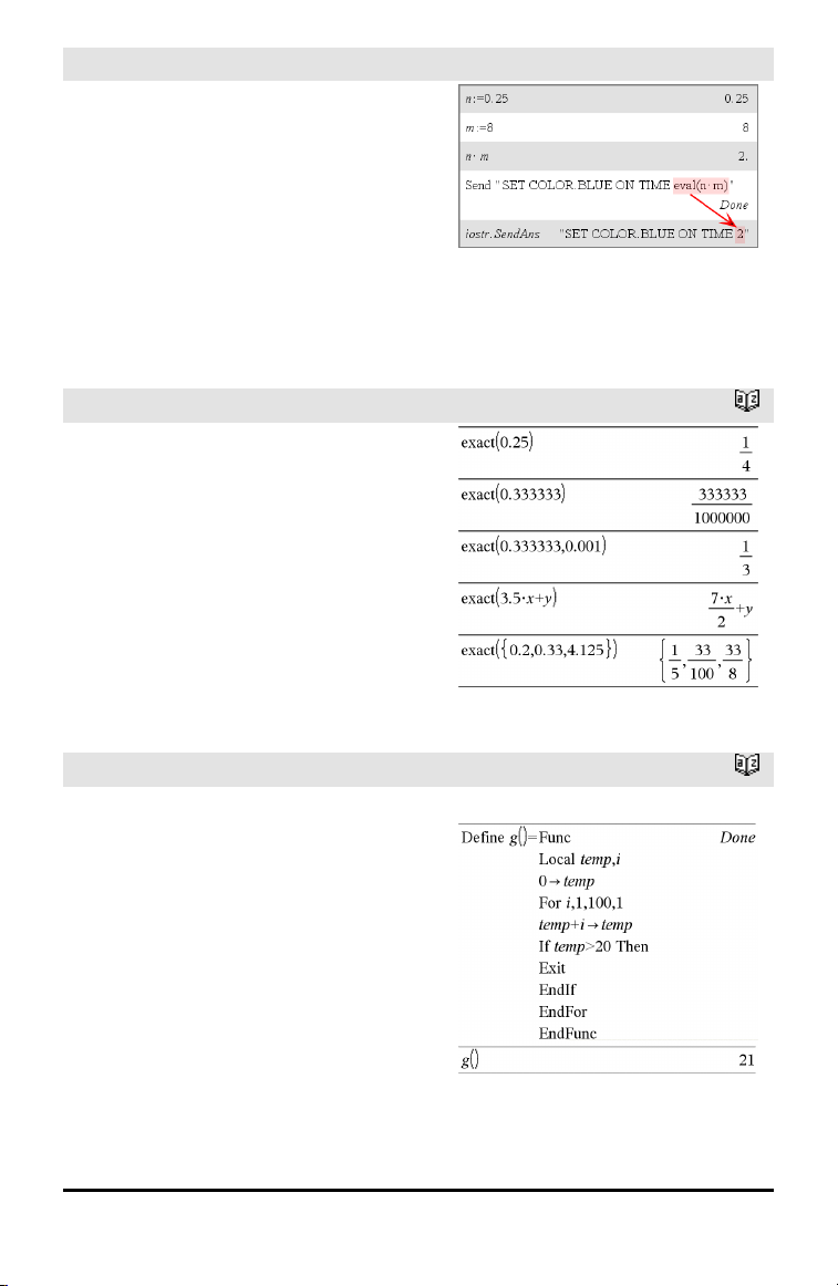
eval () Hub Menu

Although eval() does not display its result, you can view the resulting Hub command string after executing the command by inspecting any of the following special variables.

iostr.SendAns iostr.GetAns iostr.GetStrAns

Note: See also Get(page 78), GetStr(page

85), and Send(page 159).

exact()

exact(Expr1 [, Tolerance]) ⇒ expression exact(List1 [, Tolerance]) ⇒ list exact(Matrix1 [, Tolerance]) ⇒ matrix

Uses Exact mode arithmetic to return, when possible, the rational-number equivalent of the argument.

Tolerance specifies the tolerance for the

conversion; the default is 0 (zero).

Exit

Exits the current For, While, or Loop block.

Exit is not allowed outside the three looping

structures (For, While, or Loop).

Note for entering the example: For

instructions on entering multi-line program and function definitions, refer to the Calculator section of your product guidebook.

Catalog >

Function listing:

Alphabetical Listing 63

►exp

Expr►exp

Represents Expr in terms of the natural exponential e. This is a display conversion operator. It can be used only at the end of the entry line.

Note: You can insert this operator from the

computer keyboard by typing @>exp.

Catalog >

exp()

exp(Expr1) ⇒ expression

Returns e raised to the Expr1 power.

Note: See also e exponent template, page

You can enter a complex number in re polar form. However, use this form in Radian angle mode only; it causes a Domain error in Degree or Gradian angle mode.

exp(List1) ⇒ list

Returns e raised to the power of each element in List1.

exp(squareMatrix1) ⇒ squareMatrix

Returns the matrix exponential of

squareMatrix1. This is not the same as

calculating e raised to the power of each element. For information about the calculation method, refer to cos().

squareMatrix1 must be diagonalizable. The

result always contains floating-point numbers.

u key

exp►list()

exp►list(Expr,Var) ⇒ list

64 A lphabetical Listing

Catalog >

exp►list()

Examines Expr for equations that are separated by the word “or,” and returns a list containing the right-hand sides of the equations of the form Var=Expr. This gives you an easy way to extract some solution values embedded in the results of the solve(), cSolve(), fMin(), and fMax() functions.

Note: exp►list() is not necessary with the zeros() and cZeros() functions because they

return a list of solution values directly.

You can insert this function from the keyboard by typing exp@>list(...).

Catalog >

expand()

expand(Expr1 [, Var]) ⇒ expression expand(List1 [,Var]) ⇒ list expand(Matrix1 [,Var]) ⇒ matrix

expand(Expr1) returns Expr1 expanded

with respect to all its variables. The expansion is polynomial expansion for polynomials and partial fraction expansion for rational expressions.

The goal of expand() is to transform Expr1 into a sum and/or difference of simple terms. In contrast, the goal of factor() is to transform Expr1 into a product and/or quotient of simple factors.

expand(Expr1,Var) returns Expr1

expanded with respect to Var. Similar powers of Var are collected. The terms and their factors are sorted with Var as the main variable. There might be some incidental factoring or expansion of the collected coefficients. Compared to omitting Var, this often saves time, memory, and screen space, while making the expression more comprehensible.

Catalog >

Alphabetical Listing 65

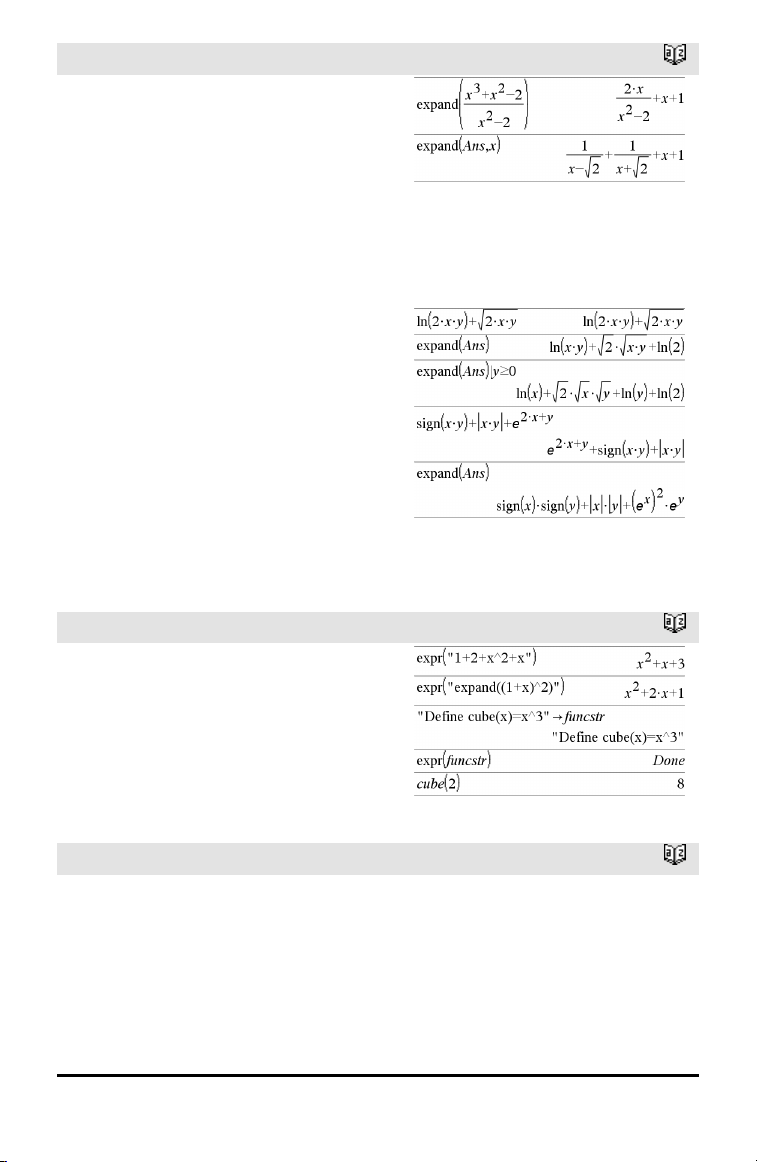
expand()

Even when there is only one variable, using

Var might make the denominator

factorization used for partial fraction expansion more complete.

Hint: For rational expressions, propFrac() is a faster but less extreme alternative to

expand().

Note: See also comDenom() for an

expanded numerator over an expanded denominator.

expand(Expr1,[Var]) also distributes

logarithms and fractional powers regardless of Var. For increased distribution of logarithms and fractional powers, inequality constraints might be necessary to guarantee that some factors are nonnegative.

expand(Expr1, [Var]) also distributes

absolute values, sign(), and exponentials, regardless of Var.

Note: See also tExpand() for trigonometric

angle-sum and multiple-angle expansion.

Catalog >

expr()

expr(String) ⇒ expression

Returns the character string contained in

String as an expression and immediately

executes it.

ExpReg

ExpReg X, Y [, [Freq] [, Category,

Include]]

Computes the exponential regression y = a• (b)xon lists X and Y with frequency Freq. A summary of results is stored in the

stat.results variable. (See page 177.)

66 A lphabetical Listing

Catalog >

ExpReg

All the lists must have equal dimension except for Include.

X and Y are lists of independent and

dependent variables.

Freq is an optional list of frequency values.

Each element in Freq specifies the frequency of occurrence for each corresponding X and Y data point. The default value is 1. All elements must be integers ≥ 0.

Category is a list of category codes for the

corresponding X and Y data.

Include is a list of one or more of the

category codes. Only those data items whose category code is included in this list are included in the calculation.

For information on the effect of empty elements in a list, see “Empty (Void) Elements,” page 236.

Catalog >

Output variable

stat.RegEqn

stat.a, stat.b Regression coefficients

stat.r

stat.r Correlationcoefficient for transformed data (x, ln(y))

stat.Resid Residuals associatedwiththe exponential model

stat.ResidTrans Residualsassociatedwithlinear fit of transformed data

stat.XReg

stat.YReg

stat.FreqReg

Description

Regression equation: a•(b)

Coefficientof linear determination for transformed data

Listof data pointsinthemodifiedX List actually used in the regression basedon restrictionsof Freq, Category List, and Include Categories

Listof data pointsinthemodifiedY List actually used in the regression basedon restrictionsof Freq, Category List, and Include Categories

Listof frequencies corresponding to stat.XReg and stat.YReg

Alphabetical Listing 67

factor()

factor(Expr1[, Var]) ⇒ expression factor(List1[,Var]) ⇒ list factor(Matrix1[,Var]) ⇒ matrix

factor(Expr1) returns Expr1 factored with

respect to all of its variables over a common denominator.

Expr1 is factored as much as possible

toward linear rational factors without introducing new non-real subexpressions. This alternative is appropriate if you want factorization with respect to more than one variable.

factor(Expr1,Var) returns Expr1 factored

with respect to variable Var.

Expr1 is factored as much as possible

toward real factors that are linear in Var, even if it introduces irrational constants or subexpressions that are irrational in other variables.

The factors and their terms are sorted with

Var as the main variable. Similar powers of Var are collected in each factor. Include Var if factorization is needed with respect

For the Auto setting of the Auto or

Approximate mode, including Var permits

approximation with floating-point coefficients where irrational coefficients cannot be explicitly expressed concisely in terms of the built-in functions. Even when there is only one variable, including Var might yield more complete factorization.

Note: See also comDenom() for a fast way

to achieve partial factoring when factor() is not fast enough or if it exhausts memory.

Catalog >

68 A lphabetical Listing

factor()

Note: See also cFactor() for factoring all the

way to complex coefficients in pursuit of linear factors.

factor(rationalNumber) returns the rational

number factored into primes. For composite numbers, the computing time grows exponentially with the number of digits in the second-largest factor. For example, factoring a 30-digit integer could take more than a day, and factoring a 100digit number could take more than a century.

To stop a calculation manually,

• Handheld: Hold down the c key and press · repeatedly.

• Windows®: Hold down the F12 key and press Enter repeatedly.

• Macintosh®: Hold down the F5 key and press Enter repeatedly.

• iPad®: The app displays a prompt. You can continue waiting or cancel.

If you merely want to determine if a number is prime, use isPrime() instead. It is much faster, particularly if rationalNumber is not prime and if the second-largest factor has more than five digits.

Catalog >

FCdf()

FCdf

(lowBound,upBound,dfNumer,dfDenom) ⇒

number if lowBound and upBound are

numbers, list if lowBound and upBound are lists

FCdf (lowBound,upBound,dfNumer,dfDenom) ⇒

number if lowBound and upBound are

numbers, list if lowBound and upBound are lists

Catalog >

Alphabetical Listing 69

FCdf()

Computes the F distribution probability between lowBound and upBound for the specified dfNumer (degrees of freedom) and

dfDenom.

For P(X ≤ upBound), set lowBound = 0.

Catalog >

Fill

Fill Expr, matrixVar ⇒ matrix

Replaces each element in variable

matrixVar with Expr.

matrixVar must already exist.

Fill Expr, listVar ⇒ list

Replaces each element in variable listVar with Expr.

listVar must already exist.

FiveNumSummary

FiveNumSummary X[,[Freq]

[,Category,Include]]

Provides an abbreviated version of the 1variable statistics on list X. Asummary of results is stored in the stat.results variable. (See page 177.)

X represents a list containing the data.

Freq is an optional list of frequency values.

Each element in Freq specifies the frequency of occurrence for each corresponding X and Y data point. The default value is 1.

Category is a list of numeric category codes

for the corresponding X data.

Include is a list of one or more of the

category codes. Only those data items whose category code is included in this list are included in the calculation.

Catalog >

70 A lphabetical Listing

FiveNumSummary

An empty (void) element in any of the lists

X, Freq, or Category results in a void for

the corresponding element of all those lists. For more information on empty elements, see page 236.

Output variable Description

stat.MinX Minimum of x values.

stat.Q1X 1stQuartile of x .

stat.MedianX Median of x .

stat.Q3X 3rd Quartileof x.

stat.MaxX Maximum of x values.

Catalog >

floor()

floor(Expr1) ⇒ integer

Returns the greatest integer that is ≤ the argument. This function is identical to int().

The argument can be a real or a complex number.

floor(List1) ⇒ list floor(Matrix1) ⇒ matrix

Returns a list or matrix of the floor of each element.

Note: See also ceiling() and int().

fMax()

fMax(Expr, Var) ⇒ Boolean expression fMax(Expr, Var,lowBound)

fMax(Expr, Var,lowBound,upBound)

fMax(Expr, Var) |

lowBound≤Var≤upBound

Returns a Boolean expression specifying candidate values of Var that maximize

Expr or locate its least upper bound.

Catalog >

Alphabetical Listing 71

fMax()

You can use the constraint (“|”) operator to restrict the solution interval and/or specify other constraints.

For the Approximate setting of the Auto or

Approximate mode, fMax() iteratively

searches for one approximate local maximum. This is often faster, particularly if you use the “|” operator to constrain the search to a relatively small interval that contains exactly one local maximum.

Note: See also fMin() and max() .

Catalog >

fMin()

fMin(Expr, Var) ⇒ Boolean expression

fMin(Expr, Var,lowBound)

fMin(Expr, Var,lowBound,upBound)

fMin(Expr, Var) |

lowBound≤Var≤upBound

Returns a Boolean expression specifying candidate values of Var that minimize

Expr or locate its greatest lower bound.

You can use the constraint (“|”) operator to restrict the solution interval and/or specify other constraints.

For the Approximate setting of the Auto or

Approximate mode, fMin() iteratively

searches for one approximate local minimum. This is often faster, particularly if you use the “|” operator to constrain the search to a relatively small interval that contains exactly one local minimum.

Note: See also fMax() and min() .

Catalog >

72 A lphabetical Listing

For

For Var, Low, High [, Step]

  Block

EndFor

Executes the statements in Block iteratively for each value of Var, from Low to High, in increments of Step.

Var must not be a system variable.

Step can be positive or negative. The

default value is 1.

Block can be either a single statement or a

series of statements separated with the “:” character.

Note for entering the example: For

instructions on entering multi-line program and function definitions, refer to the Calculator section of your product guidebook.

Catalog >

format()

format(Expr[, formatString]) ⇒ string

Returns Expr as a character string based on the format template.

Expr must simplify to a number.

formatString is a string and must be in the

form: “F[n]”, “S[n]”, “E[n]”, “G[n][c]”, where [] indicate optional portions.

F[n]: Fixed format. n is the number of digits to display after the decimal point.

S[n]: Scientific format. n is the number of digits to display after the decimal point.

E[n]: Engineering format. n is the number of digits after the first significant digit. The exponent is adjusted to a multiple of three, and the decimal point is moved to the right by zero, one, or two digits.

Catalog >

Alphabetical Listing 73

format()

G[n][c]: Same as fixed format but also separates digits to the left of the radix into groups of three. c specifies the group separator character and defaults to a comma. If c is a period, the radix will be shown as a comma.

[Rc]: Any of the above specifiers may be suffixed with the Rc radix flag, where c is a single character that specifies what to substitute for the radix point.

Catalog >

fPart()

fPart(Expr1) ⇒ expression fPart(List1) ⇒ list fPart(Matrix1) ⇒ matrix

Returns the fractional part of the argument.

For a list or matrix, returns the fractional parts of the elements.

The argument can be a real or a complex number.

FPdf()

FPdf(XVal,dfNumer,dfDenom) ⇒ number

if XVal is a number, list if XVal is a list

Computes the F distribution probability at

XVal for the specified dfNumer (degrees of

freedom) and dfDenom.

freqTable►list()

freqTable►list(List1,freqIntegerList) ⇒

list

Returns a list containing the elements from

List1 expanded according to the

frequencies in freqIntegerList. This function can be used for building a frequency table for the Data & Statistics application.

List1 can be any valid list.

Catalog >

74 A lphabetical Listing

freqTable►list()

freqIntegerList must have the same

dimension as List1 and must contain nonnegative integer elements only. Each element specifies the number of times the corresponding List1 element will be repeated in the result list. A value of zero excludes the corresponding List1 element.

Note: You can insert this function from the

computer keyboard by typing

freqTable@>list(...).

Empty (void) elements are ignored. For more information on empty elements, see page 236.

Catalog >

frequency()

frequency(List1,binsList) ⇒ list

Returns a list containing counts of the elements in List1. The counts are based on ranges (bins) that you define in binsList.

If binsList is {b(1), b(2), …, b(n)}, the specified ranges are {?≤b(1), b(1)<?≤b (2),…,b(n-1)<?≤b(n), b(n)>?}. The resulting list is one element longer than binsList.

Each element of the result corresponds to the number of elements from List1 that are in the range of that bin. Expressed in terms of the countIf() function, the result is {countIf(list, ?≤b(1)), countIf(list, b(1)<?≤b (2)), …, countIf(list, b(n-1)<?≤b(n)), countIf (list, b(n)>?)}.

Elements of List1 that cannot be “placed in a bin” are ignored. Empty (void) elements are also ignored. For more information on empty elements, see page 236.

Within the Lists & Spreadsheet application, you can use a range of cells in place of both arguments.

Note: See also countIf(), page 35.

Catalog >

Explanationof result:

2 elements from Datalist are ≤2.5

4 elements from Datalist are >2.5 and≤4.5

3 elements from Datalist are >4.5

Theelement“hello” is a string and cannot be placedinany of the defined bins.

Alphabetical Listing 75

FTest_2Samp

Catalog >

FTest_2Samp List1,List2[,Freq1[,Freq2 [,Hypoth]]]

(Data list input)

FTest_2Samp sx1,n1,sx2,n2[,Hypoth]

(Summary stats input)

Performs a two-sample Ftest. A summary of results is stored in the stat.results variable. (See page 177.)

For Ha: σ1 > σ2, set Hypoth>0 For Ha: σ1 ≠ σ2 (default), set Hypoth =0 For Ha: σ1 < σ2, set Hypoth<0

For information on the effect of empty elements in a list, see Empty (Void) Elements, page 236.

Output variable Description

stat.F CalculatedF statistic for the data sequence

stat.PVal Smallest level of significance at which thenull hypothesis can be rejected

stat.dfNumer numerator degrees of freedom = n1-1

stat.dfDenom denominator degrees of freedom = n2-1

stat.sx1, stat.sx2

stat.x1_bar stat.x2_bar

stat.n1, stat.n2 Size of the samples

Sample standarddeviations of the data sequencesinList1 and List2

Sample means of the data sequences inList1 andList2

Func

  Block

EndFunc

Template for creating a user-defined function.

76 A lphabetical Listing

Catalog >

Definea piecewisefunction:

Func

Block can be a single statement, a series

of statements separated with the “:” character, or a series of statements on separate lines. The function can use the

Return instruction to return a specific result.

Note for entering the example: For

instructions on entering multi-line program and function definitions, refer to the Calculator section of your product guidebook.

Catalog >

Resultof graphing g(x)

gcd()

gcd(Number1, Number2) ⇒ expression

Returns the greatest common divisor of the two arguments. The gcd of two fractions is the gcd of their numerators divided by the

lcm of their denominators.

In Auto or Approximate mode, the gcd of fractional floating-point numbers is 1.0.

gcd(List1, List2) ⇒ list

Returns the greatest common divisors of the corresponding elements in List1 and

List2.

gcd(Matrix1, Matrix2) ⇒ matrix

Returns the greatest common divisors of the corresponding elements in Matrix1and

Matrix2.

geomCdf()

geomCdf(p,lowBound,upBound) ⇒ number

Catalog >

Alphabetical Listing 77

geomCdf()

if lowBound and upBound are numbers, list if lowBound and upBound are lists

geomCdf(p,upBound)for P(1≤X≤upBound)

⇒ number if upBound is a number, list if upBound is a list

Computes a cumulative geometric probability from lowBound to upBound with the specified probability of success p.

For P(X ≤ upBound), set lowBound = 1.

Catalog >

geomPdf()

Catalog >

geomPdf(p,XVal) ⇒ number if XVal is a

number, list if XVal is a list

Computes a probability at XVal, the number of the trial on which the first success occurs, for the discrete geometric distribution with the specified probability of success p.

Get Hub Menu

Get [promptString,] var[,statusVar]

Get [promptString,] func(arg1, ...argn)

[,statusVar]

Programming command: Retrieves a value from a connected TI-Innovator™ Hub and assigns the value to variable var.

The value must be requested:

• In advance, through a Send"READ..." command.

—or—

• By embedding a "READ..." request as the optional promptString argument. This method lets you use a single command to request the value and retrieve it.

Example: Requestthecurrentvalueof the hub'sbuilt-inlight-level sensor. Use Get to retrieve the value and assign it to variable

lightval.

Embed theREAD requestwithin the Get command.

78 A lphabetical Listing

Get Hub Menu

Implicit simplification takes place. For example, a received string of "123" is interpreted as a numeric value. To preserve the string, use GetStr instead of Get.

If you include the optional argument

statusVar, it is assigned a value based on

the success of the operation. A value of zero means that no data was received.

In the second syntax, the func() argument allows a program to store the received string as a function definition. This syntax operates as if the program executed the command:

Define func(arg1, ...argn) = received

string

The program can then use the defined function func().

Note: You can use the Get command within

a user-defined program but not within a function.

Note: See also GetStr, page 85 and Send,

page 159.

getDenom()

getDenom(Expr1) ⇒ expression

Transforms the argument into an expression having a reduced common denominator, and then returns its denominator.

getKey()

getKey([0|1]) ⇒ returnString

Description:getKey() - allows a TI-Basic

program to get keyboard input handheld, desktop and emulator on desktop.

Example:

Catalog >

Example:

Alphabetical Listing 79

getKey()

• keypressed := getKey() will return a key or an empty string if no key has been pressed. This call will return immediately.

• keypressed := getKey(1) will wait till a key is pressed. This call will pause execution of the program till a key is pressed.

Handling of key presses:

Handheld Device/Emulator

Key

Esc Esc "esc"

Touchpad - Top click n/a "up"

On n/a "home"

Scratchapps n/a "scratchpad"

Touchpad - Left click n/a "left"

Touchpad - Center click n/a "center"

Touchpad - Right click n/a "right"

Doc n/a "doc"

Desktop Return Value

Catalog >

Tab Tab "tab"

Touchpad - Bottom click Down Arrow "down"

Menu n/a "menu"

Ctrl Ctrl no return

Shift Shift no return

Var n/a "var"

Del n/a "del"

= = "="

trig n/a "trig"

0 through 9 0-9 "0" ... "9"

80 A lphabetical Listing

Handheld Device/Emulator

Key

Desktop Return Value

Templates n/a "template"

Catalog n/a "cat"

^ ^ "^"

X^2 n/a "square"

/ (division key) / "/"

* (multiply key) * "*"

e^x n/a "exp"

10^x n/a "10power"

+ + "+"

- - "-"

( ( "("

) ) ")"

. . "."

(-) n/a "-" (negate sign)

Enter Enter "enter"

ee n/a "E" (scientific notation E)

a - z a-z alpha = letter pressed (lower

case) ("a" - "z")

shift a-z shift a-z alpha = letter pressed

"A" - "Z"

Note: ctrl-shift works to lock caps

?! n/a "?!"

pi n/a "pi"

Flag n/a no return

, , ","

Return n/a "return"

Alphabetical Listing 81

Handheld Device/Emulator

Key

Desktop Return Value

Space Space " " (space)

Inaccessible Special Character Keys like

The character is returned

@,!,^, etc.

n/a Function Keys No returned character

n/a Special desktop control keys No returned character

Inaccessible Other desktop keys that are

not available on the

Same character you get in

Notes (not in a math box) calculator while getkey() is waiting for a keystroke. ({, },;, :, ...)

Note: It is important to note that the presence of getKey() in a program changes how certain events are handled by the system. Some of these are described below.

Terminate program and Handle event - Exactly as if the user were to break out of program by pressing the ON key

"Support" below means - System works as expected - program continues to run.

Event Device Desktop - TI-Nspire™

Quick Poll Terminate program,

handle event

Student Software

Same as the handheld (TINspire™ Student Software, TI-Nspire™ Navigator™ NC Teacher Software-only)

Remote file mgmt

(Incl. sending 'Exit Press 2 Test' file from another handheld or desktop-

Terminate program, handle event

Same as the handheld. (TI-Nspire™ Student

Software, TI-Nspire™ Navigator™ NC Teacher Software-only)

handheld)

End Class Terminate program,

handle event

Support (TI-Nspire™ Student

Software, TI-Nspire™ Navigator™ NC Teacher Software-only)

Event Device Desktop - TI-Nspire™ All

TI-Innovator™ Hub connect/disconnect

Support - Can successfully issue commands to the TI-

Versions

Same as the handheld

Innovator™ Hub. After you

82 A lphabetical Listing

exit the program the TIInnovator™ Hub is still working with the handheld.

getLangInfo()

getLangInfo() ⇒ string

Returns a string that corresponds to the short name of the currently active language. You can, for example, use it in a program or function to determine the current language.

English = “en” Danish = “da” German = “de” Finnish = “fi” French = “fr” Italian = “it” Dutch = “nl” Belgian Dutch = “nl_BE” Norwegian = “no” Portuguese = “pt” Spanish = “es” Swedish = “sv”

getLockInfo()

getLockInfo(Var) ⇒ value

Returns the current locked/unlocked state of variable Var.

value =0: Var is unlocked or does not exist.

value =1: Var is locked and cannot be

modified or deleted.

See Lock, page 107, and unLock, page 197.

Catalog >

Alphabetical Listing 83

getMode()

getMode(ModeNameInteger) ⇒ value

getMode(0) ⇒ list

getMode(ModeNameInteger) returns a

value representing the current setting of the ModeNameInteger mode.

getMode(0) returns a list containing

number pairs. Each pair consists of a mode integer and a setting integer.

For a listing of the modes and their settings, refer to the table below.

If you save the settings with getMode(0) →

var, you can use setMode(var) in a function

or program to temporarily restore the settings within the execution of the function or program only. See setMode(), page 162.

Catalog >

Mode Name

Display Digits

Angle

Exponential Format

Real or Complex

Auto or Approx.

Vector Format

Base

Unit system

Mode Integer Setting Integers

1=Float, 2=Float1, 3=Float2, 4=Float3, 5=Float4, 6=Float5, 7=Float6, 8=Float7, 9=Float8, 10=Float9, 11=Float10, 12=Float11, 13=Float12, 14=Fix0, 15=Fix1, 16=Fix2, 17=Fix3, 18=Fix4, 19=Fix5, 20=Fix6, 21=Fix7, 22=Fix8, 23=Fix9, 24=Fix10, 25=Fix11, 26=Fix12

1=Radian, 2=Degree, 3=Gradian

1=Normal, 2=Scientific, 3=Engineering

1=Real, 2=Rectangular, 3=Polar

1=Auto, 2=Approximate, 3=Exact

1=Rectangular, 2=Cylindrical, 3=Spherical

1=Decimal, 2=Hex, 3=Binary

1=SI, 2=Eng/US

84 A lphabetical Listing

getNum()

getNum(Expr1) ⇒ expression

Transforms the argument into an expression having a reduced common denominator, and then returns its numerator.

Catalog >

GetStr Hub Menu

GetStr [promptString,] var[, statusVar]

GetStr [promptString,] func(arg1, ...argn)

[,statusVar]

Programming command: Operates identically to the Get command, except that the retrieved value is always interpreted as a string. By contrast, the Get command interprets the response as an expression unless it is enclosed in quotation marks ("").

Note: See also Get, page 78 and Send, page

159.

For examples, see Get.

getType()

getType(var) ⇒ string

Returns a string that indicates the data type of variable var.

If var has not been defined, returns the string "NONE".

Catalog >

Alphabetical Listing 85

getVarInfo()

getVarInfo() ⇒ matrix or string

getVarInfo(LibNameString) ⇒ matrix or

string

getVarInfo() returns a matrix of information

(variable name, type, library accessibility, and locked/unlocked state) for all variables and library objects defined in the current problem.

If no variables are defined, getVarInfo() returns the string "NONE".

getVarInfo(LibNameString)returns a matrix

of information for all library objects defined in library LibNameString. LibNameString must be a string (text enclosed in quotation marks) or a string variable.

If the library LibNameString does not exist, an error occurs.

Note the example, in which the result of

getVarInfo() is assigned to variable vs.

Attempting to display row 2 or row 3 of vs returns an “Invalid list or matrix” error because at least one of elements in those rows (variable b, for example) revaluates to a matrix.

This error could also occur when using Ans to reevaluate a getVarInfo() result.

The system gives the above error because the current version of the software does not support a generalized matrix structure where an element of a matrix can be either a matrix or a list.

Catalog >

86 A lphabetical Listing

Goto

Goto labelName

Transfers control to the label labelName.

labelName must be defined in the same

function using a Lbl instruction.

Note for entering the example: For

instructions on entering multi-line program and function definitions, refer to the Calculator section of your product guidebook.

Catalog >

►Grad

Expr1►Grad ⇒ expression

Converts Expr1 to gradian angle measure.

Note: You can insert this operator from the

computer keyboard by typing @>Grad.

identity()

identity(Integer) ⇒ matrix

Returns the identity matrix with a dimension of Integer.

Integer must be a positive integer.

If BooleanExpr

Statement

If BooleanExpr Then

Block

EndIf

Catalog >

In Degree angle mode:

In Radian angle mode:

Catalog >

Alphabetical Listing 87

If BooleanExpr evaluates to true, executes the single statement Statement or the block of statements Block before continuing execution.

If BooleanExpr evaluates to false, continues execution without executing the statement or block of statements.

Block can be either a single statement or a

sequence of statements separated with the “:” character.

Note for entering the example: For

instructions on entering multi-line program and function definitions, refer to the Calculator section of your product guidebook.

If BooleanExpr Then

  Block1

Else

  Block2

EndIf

If BooleanExpr evaluates to true, executes

Block1 and then skips Block2.

If BooleanExpr evaluates to false, skips

Block1 but executes Block2.

Block1 and Block2 can be a single

statement.

If BooleanExpr1 Then

  Block1

ElseIf BooleanExpr2 Then

  Block2

⋮

ElseIf BooleanExprN Then

  BlockN

EndIf

Allows for branching. If BooleanExpr1 evaluates to true, executes Block1. If

BooleanExpr1 evaluates to false, evaluates BooleanExpr2, and so on.

Catalog >

88 A lphabetical Listing

ifFn()

ifFn(BooleanExpr,Value_If_true [,Value_

If_false [,Value_If_unknown]]) ⇒ expression, list, or matrix

Evaluates the boolean expression

BooleanExpr (or each element from BooleanExpr ) and produces a result based

on the following rules:

• BooleanExpr can test a single value, a list, or a matrix.

• If an element of BooleanExpr evaluates to true, returns the corresponding element from Value_If_true.

• If an element of BooleanExpr evaluates to false, returns the corresponding element from Value_If_false. If you omit Value_If_false, returns undef.

• If an element of BooleanExpr is neither true nor false, returns the corresponding element Value_If_unknown. If you omit

Value_If_unknown, returns undef.

• If the second, third, or fourth argument of the ifFn() function is a single expression, the Boolean test is applied to every position in BooleanExpr.

Note: If the simplified BooleanExpr

statement involves a list or matrix, all other list or matrix arguments must have the same dimension(s), and the result will have the same dimension(s).

Catalog >

Testvalue of 1 isless than2.5, so its corresponding

Value_If_True elementof 5 is copied to

the result list.

Testvalue of 2 isless than2.5, so its corresponding

Value_If_True elementof 6 is copied to

the result list.

Testvalue of 3 isnot less than2.5, so its corresponding Value_If_Fa lse element of

10 is copied to the result list.

Value_If_true is a singlevalueand

corresponds to any selected position.

Value_If_false is not specified. Undef is

used.

imag()

imag(Expr1) ⇒ expression

Returns the imaginary part of the argument.

One elementselectedfrom Value_If_true. One elementselectedfrom Value_If_

unknown.

Catalog >

Alphabetical Listing 89

imag()

Note: All undefined variables are treated as

real variables. See also real(), page 147

imag(List1) ⇒ list

Returns a list of the imaginary parts of the elements.

imag(Matrix1) ⇒ matrix

Returns a matrix of the imaginary parts of the elements.

Catalog >

impDif()

impDif(Equation, Var, dependVar[,Ord])

⇒ expression

where the order Ord defaults to 1.

Computes the implicit derivative for equations in which one variable is defined implicitly in terms of another.

Indirection

inString()

inString(srcString, subString[, Start]) ⇒

integer

Returns the character position in string

srcString at which the first occurrence of

string subString begins.

Start, if included, specifies the character

position within srcString where the search begins. Default = 1 (the first character of

srcString).

If srcString does not contain subString or

Start is > the length of srcString, returns

zero.

Catalog >

See #(), page 226.

Catalog >

90 A lphabetical Listing

int()

int(Expr) ⇒ integer

int(List1) ⇒ list int(Matrix1) ⇒ matrix

Returns the greatest integer that is less than or equal to the argument. This function is identical to floor().

The argument can be a real or a complex number.

For a list or matrix, returns the greatest integer of each of the elements.

Catalog >

intDiv()

intDiv(Number1, Number2) ⇒ integer intDiv(List1, List2) ⇒ list intDiv(Matrix1, Matrix2) ⇒ matrix

Returns the signed integer part of (Number1 ÷ Number2).

For lists and matrices, returns the signed integer part of (argument1÷argument2) for each element pair.

integral

interpolate ()

interpolate(xValue, xList, yList,

yPrimeList) ⇒ list

This function does the following:

Catalog >

See ∫(), page 221.

Catalog >

Differentialequation:

y'=-3•y+6•t+5andy(0)=5

To see the entire result, press £ and then use¡and¢ to move thecursor.

Alphabetical Listing 91

interpolate ()

Given xList, yList=f(xList), and

yPrimeList=f'(xList) for some unknown

function f, a cubic interpolant is used to approximate the function f at xValue. It is assumed that xList is a list of monotonically increasing or decreasing numbers, but this function may return a value even when it is not. This function walks through xList looking for an interval [xList[i], xList[i+1]] that contains xValue. If it finds such an interval, it returns an interpolated value for f(xValue); otherwise, it returns undef.

xList, yList, and yPrimeList must be of

equal dimension ≥ 2 and contain expressions that simplify to numbers.

xValue can be an undefined variable, a

number, or a list of numbers.

Catalog >

Use the interpolate() functionto calculatethe function values for the xvaluelist:

invχ2()

invχ2(Area,df)

invChi2(Area,df)

Computes the Inverse cumulative χ2(chisquare) probability function specified by degree of freedom, df for a given Area under the curve.

invF()

invF(Area,dfNumer,dfDenom)

computes the Inverse cumulative F distribution function specified by dfNumer and dfDenom for a given Area under the curve.

Catalog >

92 A lphabetical Listing

invBinom()

invBinom (CumulativeProb,NumTrials,Prob,

OutputForm)⇒ scalar or matrix

Inverse binomial. Given the number of trials (NumTrials) and the probability of success of each trial (Prob), this function returns the minimum number of successes, k, such that the value, k, is greater than or equal to the given cumulative probability (CumulativeProb).

OutputForm=0, displays result as a scalar

(default).

OutputForm=1, displays result as a matrix.

Catalog >

Example: Mary andKevinare playinga dice game. Mary hasto guess the maximum number of times 6 showsupin30 rolls. If the number 6 shows upthatmany timesor less, Mary wins. Furthermore, thesmaller the number that she guesses, the greater her winnings. What is the smallest number Mary canguess if she wantstheprobability of winning to be greater than 77%?

invBinomN()

invBinomN(CumulativeProb,Prob,

NumSuccess,OutputForm)⇒ scalar or

matrix

Inverse binomial with respect to N. Given the probability of success of each trial (Prob), and the number of successes (NumSuccess), this function returns the minimum number of trials, N, such that the value, N, is less than or equal to the given cumulative probability (CumulativeProb).

OutputForm=0, displays result as a scalar

(default).

OutputForm=1, displays result as a matrix.

invNorm()

invNorm(Area[,μ[,σ]])

Computes the inverse cumulative normal distribution function for a given Area under the normal distribution curve specified by μ and σ.

invt()

invt(Area,df)

Catalog >

Example: Monique is practicing goal shots for netball. She knows from experience that her chance of making any one shot is70%. She plansto practice until she scores 50 goals. How many shots mustshe attemptto ensure thattheprobability of making at least 50 goals is more than0.99?

Catalog >

Alphabetical Listing 93

invt()

Computes the inverse cumulative student-t probability function specified by degree of freedom, df for a given Area under the curve.

Catalog >

iPart()

iPart(Number) ⇒ integer

iPart(List1) ⇒ list iPart(Matrix1) ⇒ matrix

Returns the integer part of the argument.

For lists and matrices, returns the integer part of each element.

The argument can be a real or a complex number.

irr()

irr(CF0,CFList [,CFFreq]) ⇒ value

Financial function that calculates internal rate of return of an investment.

CF0 is the initial cash flow at time 0; it

must be a real number.

CFList is a list of cash flow amounts after

the initial cash flow CF0.

CFFreq is an optional list in which each

element specifies the frequency of occurrence for a grouped (consecutive) cash flow amount, which is the corresponding element of CFList. The default is 1; if you enter values, they must be positive integers < 10,000.

Note: See also mirr(), page 116.

Catalog >

isPrime()

isPrime(Number) ⇒ Boolean constant

expression

94 A lphabetical Listing

Catalog >

isPrime()

Returns true or false to indicate if number is a whole number ≥2 that is evenly divisible only by itself and 1.

If Number exceeds about 306 digits and has no factors ≤1021, isPrime(Number) displays an error message.

If you merely want to determine if Number is prime, use isPrime() instead of factor(). It is much faster, particularly if Number is not prime and has a second-largest factor that exceeds about five digits.

Note for entering the example: For

instructions on entering multi-line program and function definitions, refer to the Calculator section of your product guidebook.

Catalog >

Function to findthe next prime after a specifiednumber:

isVoid()

isVoid(Var) ⇒ Boolean constant

expression

isVoid(Expr) ⇒ Boolean constant

expression

isVoid(List) ⇒ list of Boolean constant

expressions

Returns true or false to indicate if the argument is a void data type.

For more information on void elements, see page 236.

Catalog >

Alphabetical Listing 95

Lbl

Lbl labelName

Defines a label with the name labelName within a function.

You can use a Goto labelName instruction to transfer control to the instruction immediately following the label.

labelName must meet the same naming

requirements as a variable name.

Note for entering the example: For

instructions on entering multi-line program and function definitions, refer to the Calculator section of your product guidebook.

lcm()

lcm(Number1, Number2) ⇒ expression lcm(List1, List2) ⇒ list lcm(Matrix1, Matrix2) ⇒ matrix

Returns the least common multiple of the two arguments. The lcm of two fractions is the lcm of their numerators divided by the

gcd of their denominators. The lcm of

fractional floating-point numbers is their product.

For two lists or matrices, returns the least common multiples of the corresponding elements.

Catalog >

left()

left(sourceString[, Num]) ⇒ string

Returns the leftmost Num characters contained in character string sourceString.

If you omit Num, returns all of

sourceString.

left(List1[, Num]) ⇒ list

96 A lphabetical Listing

Catalog >

Texas Instruments TI-Nspire CX CAS Reference Guide

Specifications and Main Features

Frequently Asked Questions

User Manual

Important Information

Expression Templates

Alphabetical Listing