Teledyne SDA III User Manual

Operator's
Manual

SDAIII-CompleteLinQ
Software

SDAIII-CompleteLinQ Software Operator's Manual

© 2013 Teledyne LeCroy, Inc. All rights reserved.

Unauthorized duplication of Teledyne LeCroy documentation materials other than for internal sales and
distribution purposes is strictly prohibited. However, clients are encouraged to distribute and duplicate
Teledyne LeCroy documentation for their own internal educational purposes.

SDAIII-CompleteLinQ and Teledyne LeCroy are registered trademarks of Teledyne LeCroy, Inc. Windows
is a registered trademark of Microsoft Corporation. Other product or brand names are trademarks or
requested trademarks of their respective holders. Information in this publication supersedes all earlier
versions. Specifications are subject to change without notice.

921143 Rev A
May 2013

Operator's Manual

TABLE OF CONTENTS

SDAIII-CompleteLinQ Overview 3

Key Features 4
What's New in SDAIII-CompleteLinQ 4
Compatible Oscilloscope Models 5
Required Firmware 5

Getting Started with SDAIII-CompleteLinQ 6

How to Order SDAIII-CompleteLinQ Capabilities 6
Accessing SDAIII-CompleteLinQ 7
SDAFramework Dialog 8
LaneScape Comparison Mode 10
Quick View 12
Lane Configuration Process 13

Signal Inputs 15

Set Up Signal 15
Signal Dialog 16
Serial Data Inputs 17
Crossing Levels 17
Signal Types 18

Clock 19

Set Up Clock Recovery 19
Clock Recovery Dialog 19
PLL Setup 20
Clock Recovery Theory 23
Set Up Reference Clock 24

Eye Measurements 26

Eye Measurements Overview 26
Eye Dialog 27
Set Up Eye Diagram 27
Eye Diagram Configuration Dialog 28
Eye Modes 29
Mask Testing 29
Mask Margin 30
Eye Parameters Dialog 31
Eye Measurement Parameters 31
Eye Analysis Theory 34

Jitter Measurements 36

Set Up Jitter Measurements 36
Jitter Filter 39
Jitter Pattern Analysis 39
Jitter Track 42
Jitter Spectrum 42
Jitter Histogram Analysis 46

921143 Rev A

1

SDAIII-CompleteLinQ Software

Jitter Parameters 47

Vertical Noise Measurements 48

Vertical Noise Measurements Overview 48
Noise Filter 49
Noise Pattern Analysis 50
Noise Track 51
Noise Spectrum 52
Noise Histogram Analysis 52
Noise Parameters 53
Noise Measurement Theory 53

Crosstalk Measurements 55

Crosstalk Analysis 55

2

921143 Rev A

Operator's Manual

SDAIII-CompleteLinQ Overview

The SDAIII-CompleteLinQ Serial Data Analysis package introduced with firmware version 6.9.0.x provides
comprehensive measurement capabilities for evaluating high-speed serial data signals.

SDAIII-CompleteLinQ builds on the power of SDAII, extending the analysis to up-to-4 lanes simul­taneously, and providing a "reference" analysis lane for comparison purposes. SDAIII-CompleteLinQ is
the single-lane version. Both packages are a signal integrity analysis framework, integrating capabilities
from the EyeDoctor II, VirtualProbe and Crosstalk packages. In this manual, SDAIII-CompleteLinQ will
often be used to refer to the underlying analysis "engine"

Like its predecessor SDAII, SDAIII-CompleteLinQ operates by rapidly processing a long signal acquisition.
For best results, acquisitions should be long enough to include at least 100,000 UI of the signal under test
(500,000 UI or more is optimal). By using long acquisitions, users can have the best statistics for accurate
measurements and be able to measure low-frequency periodic jitter components.

The calculation methodology in SDAIII-CompleteLinQ is the same as SDAII, with the addition of the Dual­Dirac "RjDirect" jitter calculation method. All jitter measurements, eye diagrams and analysis views are
based on comparisons of the arrival times of the signals edges to that of the underlying clock, which is
determined either via a software clock recovery algorithm or by measurement of a clock signal. Nothing
is measured relative to the trigger; as a result, measurements are not affected by trigger jitter.

SDAIII-CompleteLinQ can be purchased as part of the standard installation on new instruments or as an
upgrade to existing instruments. See How to Order SDAIII-CompleteLinQ Capabilities.

921143 Rev A

3

SDAIII-CompleteLinQ Software

Key Features

l Simultaneous analysis of up-to-four lanes of data (requires one of the LinQ options).

l Two overall types of measurements: eye pattern testing and comprehensive jitter analysis (includ-

ing random and deterministic jitter separation, and direct measurement of periodic jitter, DDj,
and DCD).

l Many plot types for jitter and eye diagram analysis, including eye diagram, IsoBER, DDj Plot, dig-

ital pattern, DDj Histogram, jitter track, PLL track, jitter spectrum (with peak annotation), spec­trum threshold, Pj Inverse FFT, jitter histogram, CDF, bathtub and Normalized Q-scale fit.

l Filtered jitter processes the time interval error trend versus time with a user-selectable band-pass

filter. This feature allows applying filters in addition to the high-pass filtering effect of the clock
recovery PLL, which is required for some serial data specifications.

l IsoBER displays the extrapolated lines of constant Bit Error Ratio down to the BER of interest on an

eye diagram.

l Quick View provides a shortcut displaying the eye diagram, TIE track, bathtub curve, jitter his-

togram, NQ-scale cursors, and jitter spectrum all on the screen at the same time.

l Fully-integrated multi-lane analysis framework with the SDAIII-CompleteLinQ LinQ family of

options, accessing features of the EyeDoctor II and VirtualProbe packages. (Single-lane analysis is
standard with SDAIII-CompleteLinQ.)

l Access to the new Reference Lane capability.

l When purchased with the Crosstalk or CrossLinQ package, access to advanced noise and crosstalk

measurements.

What's New in SDAIII-CompleteLinQ

Fully-integrated, Multi-lane Analysis Framework

The SDAIII-CompleteLinQfamily of software options begins with a configuration dialog that integrates all
the serial data analysis capabilities enabled on your oscilloscope. Buttons for emphasis, equalization, de­embedding and emulation are enabled with the EyeDoctor II package. The Noise and Crosstalk buttons
are enabled by the Crosstalk and CrossLinQ packages.

Multi-lane Serial Data Analysis

When ordering SDAIII-CompleteLinQ capabilities, you can enable up-to-4 lanes for analysis. Lanes can use
either single-ended or differential signals, or be directly cabled to the oscilloscope using probes or other
waveforms traces including zooms, math functions or memory traces. You can configure lanes to analyze
data from different inputs, or can utilize multi-lane analysis to perform different analysis on the same
data. (For example, all lanes could use channels 1 and 2 as the source data, with different configurations
for the jitter analysis, such as different jitter filter settings or jitter calculation methods.) Ifyou also use
EyeDoctor II, you can configure different equalization schemes on each lane.

Noise and Crosstalk Measurements

When purchasing either the SDAIII-CompleteLinQ-Crosstalk or SDAIII-CompleteLinQ-CrossLinQ package,
you have access to the Noise and Crosstalk measurements. This powerful measurement package char­acterizes vertical noise, providing insight into noise due to crosstalk or interference. The set of analysis
views is similar to what is found in SDAIII-CompleteLinQ jitter measurements, and includes residual noise

4

921143 Rev A

Operator's Manual

track, noise spectrum, histogram and Q-fit, and noise measurements broken down into Tn (total noise),
Rn (random noise) and Dn (deterministic noise). The Crosstalk package includes the Crosstalk Eye, which
is an eye diagram based on noise analysis that depicts effects from noise aggressors more clearly than a
standard eye diagram. You can compare Crosstalk Eyes from 2 different lanes.

LaneScape Comparison Mode

When you enable multiple lanes (or one lane + the Reference lane), the oscilloscope automatically turns
on "LaneScape Comparison Mode". In this mode, all waveforms and traces for a single lane are displayed
in its own frame, which you can arrange into different "LaneScapes." You can choose to display one, two
or all LaneScapes at a time to meet your particular needs for comparing analysis results between lanes.

Spectral Rj Direct Jitter Calculation Method

SDAIII-CompleteLinQ includes the Spectral Rj Direct jitter calculation method. This method fixes Rj based
spectral analysis methods, and can return jitter results that compare more closely to results on oscil­loscopes from other manufacturers. See Understanding SDAIII-CompleteLinQ Jitter Calculation Methods
for more information.

Compatible Oscilloscope Models

The SDAIII-CompleteLinQfamily of software options is available on the WavePro/SDA/DDA 7 Zi/Zi-A,
WaveMaster/SDA/DDA 8 Zi/Zi-A, LabMaster 9 Zi-A and LabMaster 10 Zi oscilloscopes platforms.

Required Firmware

Your oscilloscope must be running firmware version 6.9.0.x or higher to support SDAIII-CompleteLinQ
and VirtualProbe. Firmware upgrades are available from www.teledynelecroy.com/support/downloads.

921143 Rev A

5

SDAIII-CompleteLinQ Software

Getting Started with SDAIII-CompleteLinQ

How to Order SDAIII-CompleteLinQ Capabilities

SDAIII-CompleteLinQcapabilities can be purchased in a variety of ways. See the product brochure on the
Teledyne LeCroy website for product names and additional ordering information, or contact your local
Teledyne LeCroy Customer Care Center.

New Oscilloscopes

SDA AND DDA MODELS

Basic SDAIII-CompleteLinQ capabilities—single-lane +reference lane, eye and jitter analysis—are deliv­ered standard with SDA/DDA 7 Zi/Zi-A and SDA/DDA 8 Zi/Zi-A oscilloscopes. To order advanced features,
attach any of the following suffixes to the scope prefix (e.g., SDA8Zi-<suffix>):

Crosstalk: Upgrades SDA or DDA models to also include noise and crosstalk measurements

LinQ:Upgrades SDA or DDAmodels to also include multi-lane eye and jitter analysis

CrossLinQ: Upgrades SDA or DDAmodels to also include multi-lane eye, jitter, noise and crosstalk anal-

ysis

CompleteLinQ: Upgrades SDA or DDAmodels to also include multi-lane eye, jitter, noise and crosstalk
analysis, and bundles in the EyeDoctor II and VirtualProbe packages.

NON-SDA AND DDA MODELS

Models in the WavePro 7 Zi/Zi-A, WaveMaster 8 Zi/Zi-A, LabMaster 9 Zi-A and LabMaster 10 Zi series can
be upgraded to include SDAIII-CompleteLinQ capabilities by ordering with the following suffixes (e.g.,
WM8Zi-<suffix>):

SDAIII: Enables single-lane +reference lane, eye and jitter analysis.

SDAIII-Crosstalk: Enables single-lane +reference lane, eye, jitter, noise and crosstalk analysis.

SDAIII-LinQ:Enables multi-lane eye and jitter analysis.

SDAIII-CrossLinQ: Enables multi-lane eye, jitter, noise and crosstalk analysis.

SDAIII-CompleteLinQ: Enables multi-lane eye, jitter, noise and crosstalk analysis, and bundles in the Eye-

Doctor II and VirtualProbe packages.

Upgrading Existing Oscilloscopes

Contact your local Teledyne LeCroy Customer Care Center for obtaining a quotation for upgrading pre­viously purchased oscilloscopes to include SDAIII-CompleteLinQ capability.

6

921143 Rev A

Operator's Manual

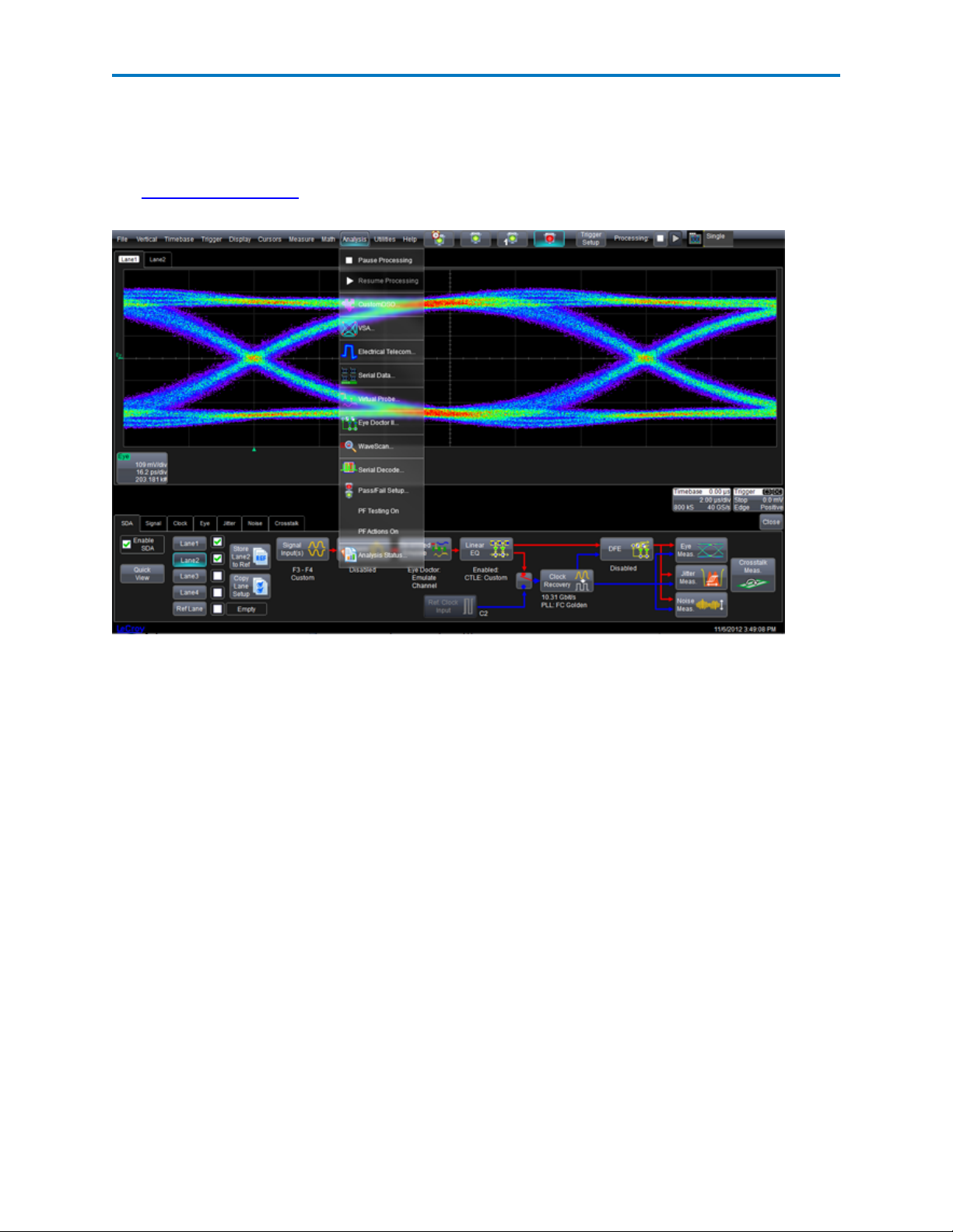
Accessing SDAIII-CompleteLinQ

Access the SDAIII-CompleteLinQ by choosing Analysis>Serial Data to display the SDA Framework dialog
at the bottom of the screen.

The SDA Framework Dialog shows the overall flow for viewing and analyzing serial data. Each block in the
flow diagram is a button that, when touched, displays its corresponding dialog.

921143 Rev A

7

SDAIII-CompleteLinQ Software

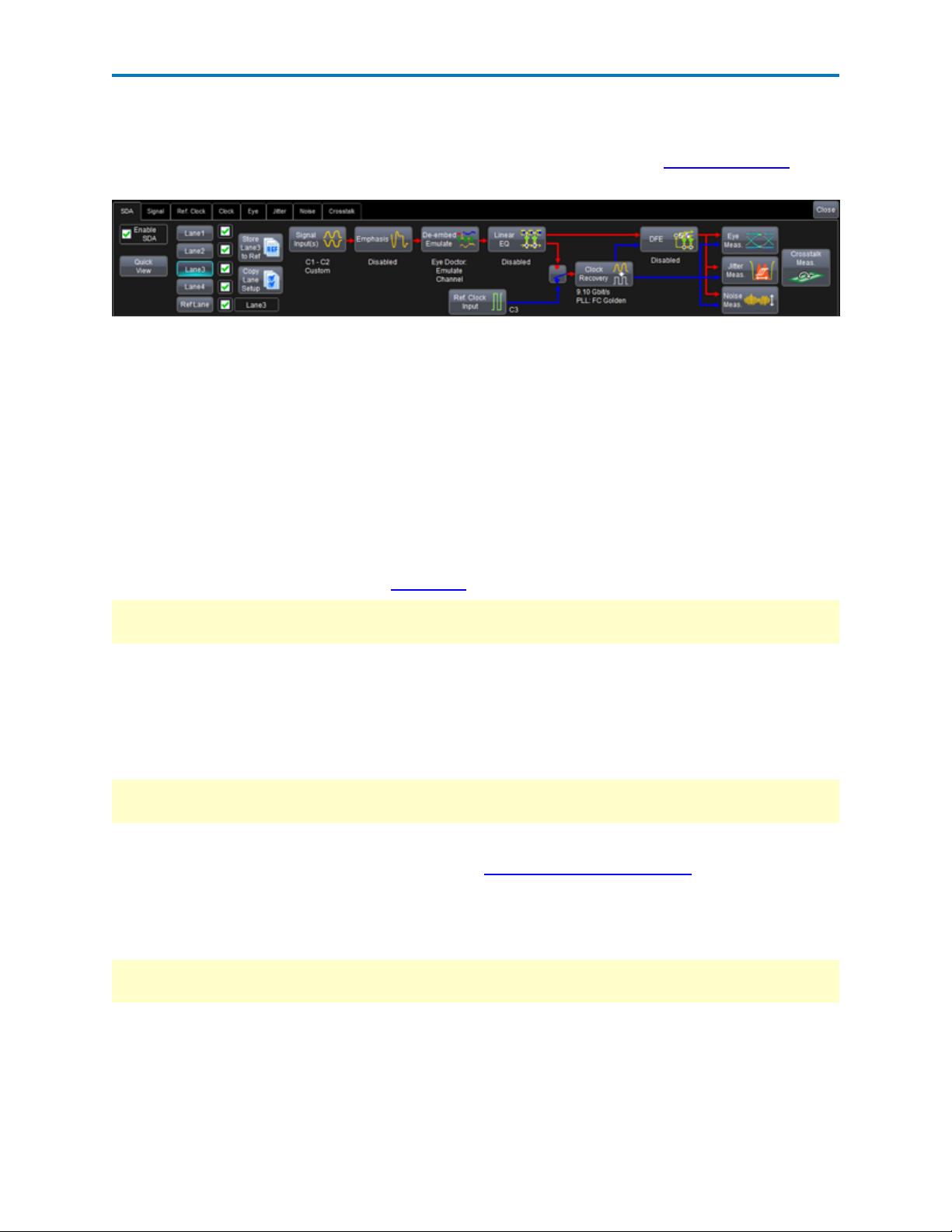
SDAFramework Dialog

This SDAIII-CompleteLinQ Framework dialog is the main configuration screen for all serial data analysis. It
represents the overall flow for viewing and analyzing serial data, beginning with lane configuration at the
left, through Eye, Jitter, Vertical Noise and Crosstalk measurement at the right.

Each block in the flow diagram is a button that, when touched, displays its corresponding configuration
dialog. Some options will be enabled or disabled depending on your SDAIII-CompleteLinQ installation.

The Framework dialog is invoked by choosing Analysis > Serial Data from the menu bar.

Integrated Operation

If you're using Eye Doctor II or VirtualProbe in conjunction with SDAIII-CompleteLinQ, use the Frame­work dialog to configure emphasis, de-embedding/emulation and equalization for the active lane.

Dialog Elements

Enable SDA checkbox - By default checked to enable all views and analyses selected within the SDAIII­CompleteLinQ environment. Unchecking this box will globally disable analysis and turn off all views.

Quick View button - Touch to open the Quick View to configure lane settings.

CAUTION:Using Quick View will clear the current configuration of the selected lane and instead apply the

configuration made within the Quick view window.

Lane 1-4 selector buttons - Touch to activate the lane for configuration. The text displayed beneath each
button in the SDA dialog gives information about the setup for the selected lane.

Ref Lane button - Touch to display the reference lane. This lane stores the data and views from another
lane for comparison purposes (see Store Lane to Ref button below). The name of the stored lane appears
to the right of the button when in use.

NOTE: The Reference Lane is unavailable for use when you enable VirtualProbe capabilities on the De­embed/Emulate dialog.

Lane Enable/Disable checkboxes - Check to enable the corresponding lane for display/analysis. When
multiple lanes are checked, the oscilloscope will enter LaneScape Comparison Mode and display each
lane in its own frame, and the Comparison Mode selection box will be active at the top right of the
screen.

Store Lane to Ref button - Touch to store the setup and data of the active lane to the reference lane.

NOTE:When VirtualProbe is enabled within the De-embed/Emulate dialog, the reference lane is unavail-

able, and the Store Lane to Ref button is disabled.

Copy Lane Setup button - Touch to open a window for copying the setup and data from one lane to
another.

8

921143 Rev A

Operator's Manual

Signal Input button - Touch to open the Signal dialog, which is used to configure settings for the active
lane including the data source(s), crossing level and signal type, and to enable the display of signal that
"flows"to the Emphasis block of the SDA flowchart.

Emphasis button - Touch to open the Emphasis dialog, which is used to configure pre-emphasis/de­emphasis settings for the signal that flows from the Signal Input(s) block. This button is enabled when
the EyeDoctor II option is present on the oscilloscope. For more information, see Emphasis Overview.

De-embed/Emulate button - Touch to open the De-embed/Emulate dialog, which is used either to con­figure fixture and channel de-embedding/emulation, or to enable the VirtualProbe option for the active
lane. This button is enabled when the EyeDoctor II option is present on the oscilloscope. For more infor­mation, see Emulate / De-embed Overview.

Linear EQ button - Touch to open the Linear EQ dialog, where you can apply CTLE(Continuous Time Lin­ear Equalization) or FFE(Feed-forward Equalization) to the active lane. This button is enabled when the
EyeDoctorII option is present on the oscilloscope. For more information, see Continuous Time Linear

Equalization (CTLE) and FeedForward Equalization (FFE).

DFE button - Touch to open the DFE(Decision Feedback Equalization) configuration window for the
active lane. This button is enabled when the EyeDoctorII option is present on the oscilloscope. For more
information, see Decision Feedback Equalizer (DFE) Configuration.

Clock Recovery Source switch - This unlabeled button is located immediately to the left of the Clock
Recovery button. When using an explicit reference clock, set the Clock Recovery Source switch to the
"Blue"position to enable the Ref Clock Input button.In this position, the clock recovery uses transitions
of the reference clock input. When set to the "Red" position, SDAIII-CompleteLinQ will perform a soft­ware clock recovery using edges from the signal flowing out of the Linear EQ box. In either position, the
settings configured in the Clock dialog are utilized.

Clock Recovery button - Touch to access the Clock dialog.

Ref Clock Input button - When using an explicit reference clock, set the clock recovery switch to the

"Blue" position to enable the Ref Clock Input button. Then, touch Ref Clock Input to open the dialog for
configuring the source and other attributes of the reference clock.

Eye Meas. button - Touch to open the dialog for configuring Eye diagram measurements for the active
lane. For more information, see Eye Measurements Overview.

Jitter Meas. button - Touch to open the dialog for configuring jitter measurements for the active lane.
For more information see Jitter Measurements Overview.

Noise Meas. button - Touch to open the dialog for the configuration of vertical noise measurements. For
more information, see Vertical Noise Measurements Overview. This button is enabled when the Cross-
talk option is present on the oscilloscope.

Crosstalk Meas. button - Touch to open the dialog for configuration of the CrosstalkEye. This button is
enabled when the Crosstalk option is present on the oscilloscope. For more information, see Crosstalk

Analysis.

921143 Rev A

9

SDAIII-CompleteLinQ Software

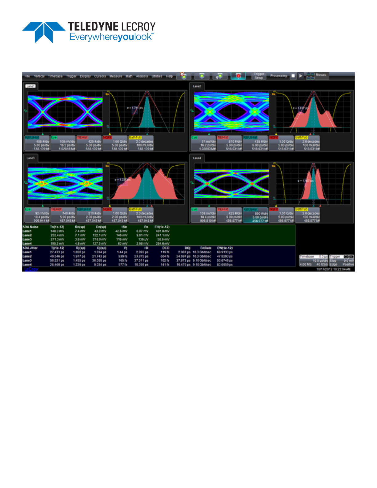
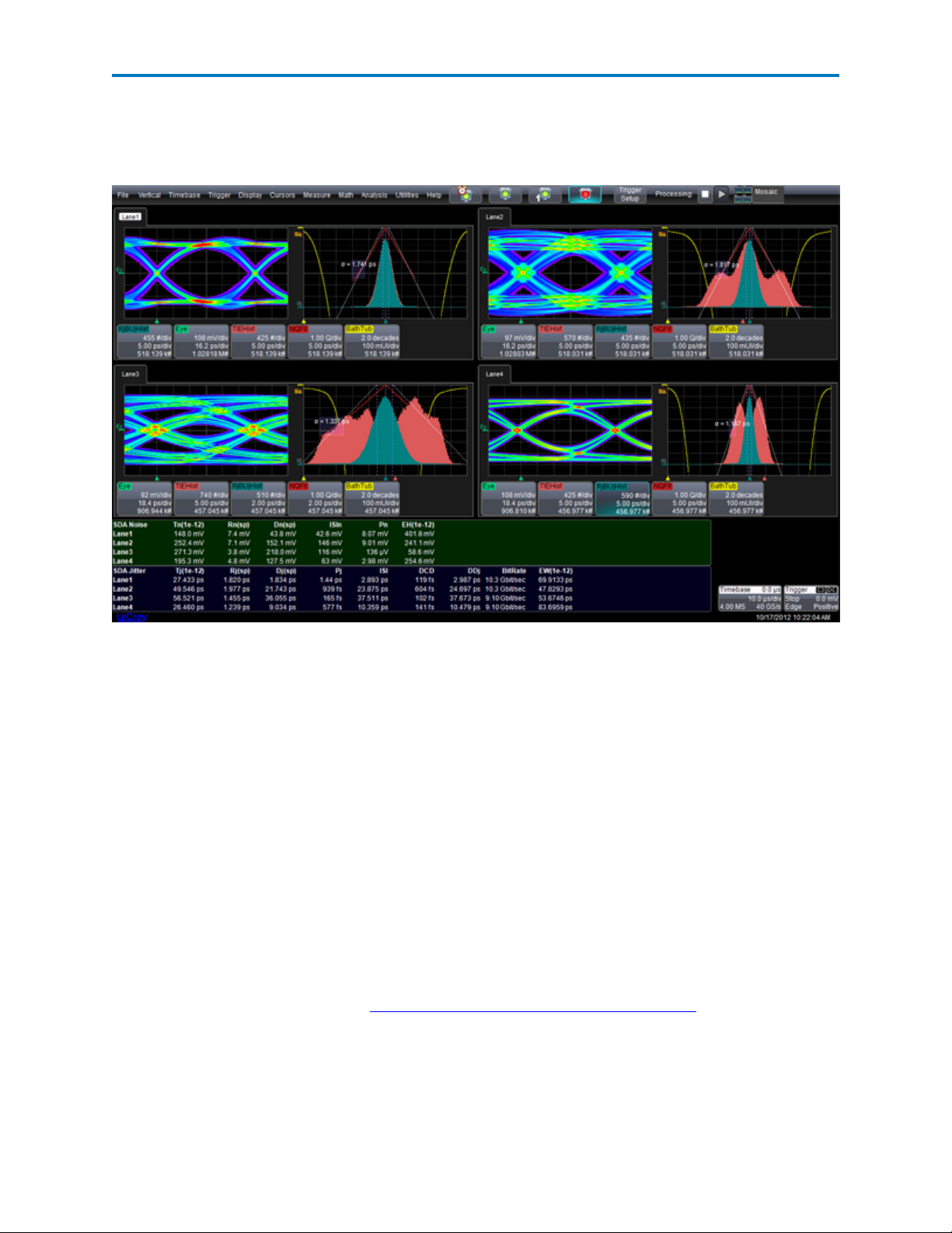
LaneScape Comparison Mode

When multiple lanes are enabled for display/analysis, the oscilloscope activates LaneScape Comparison
mode. In this mode, waveforms and views for each lane are placed in separate frames, which you can
arrange into different "LaneScapes" to facilitate analysis. Waveforms and views are synchronized
between LaneScapes.

Selecting a LaneScape Mode

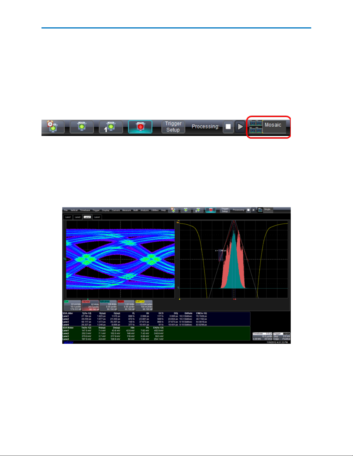
When multiple lanes are enabled, the Comparison Mode selector is displayed at the far right of the appli­cation menu bar.

Touch the icon or text to open the selector to choose a LaneScape mode.

LaneScape Modes

You can choose from three LaneScape modes:

Single - One LaneScape is displayed, allowing maximum screen area for viewing the analysis of a single
lane. If multiple lanes are enabled, tabs for each lane/frame appear above the grid; select the tab for the
frame you wish to display in the LaneScape.

10

921143 Rev A

Operator's Manual

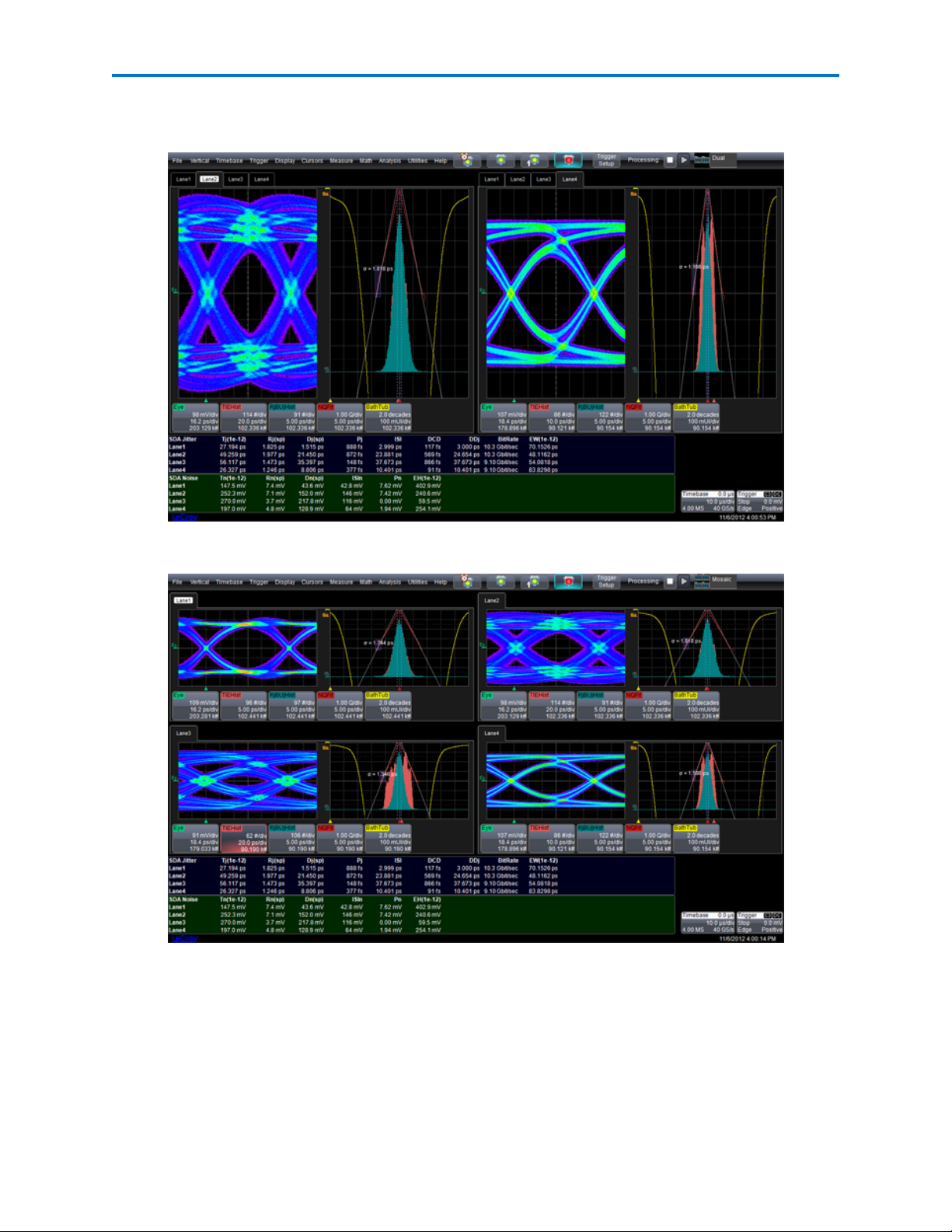
Dual - Two LaneScapes are shown side-by-side. Tabs for selecting lanes/frames appear above the grid in
both LaneScapes.

Mosaic - All enabled lanes/frames are displayed in their own LaneScapes (up to four).

921143 Rev A

11

SDAIII-CompleteLinQ Software

Assignment of Traces to LaneScapes

LaneScape mode is architected to facilitate easy comparison of SDAIII-CompleteLinQ results for multiple
lanes. To prevent misinterpretation of results, the waveform for each lane can only be displayed in its
own frame.

Non-SDAIII-CompleteLinQ waveforms, such as input channels, math functions, zooms and memory
traces (C1, F1, Z1, M1, etc.) are not locked to a frame and can be moved from one LaneScape to another.
To move a trace to a different LaneScape, do one of the following:

l Touch the trace to open the context menu, then select "Next LaneScape" to move the trace.

l When using a mouse, right-click on a descriptor box to open the context menu, then select "Next

LaneScape."

l Drag the descriptor box for the trace to the desired LaneScape and grid.

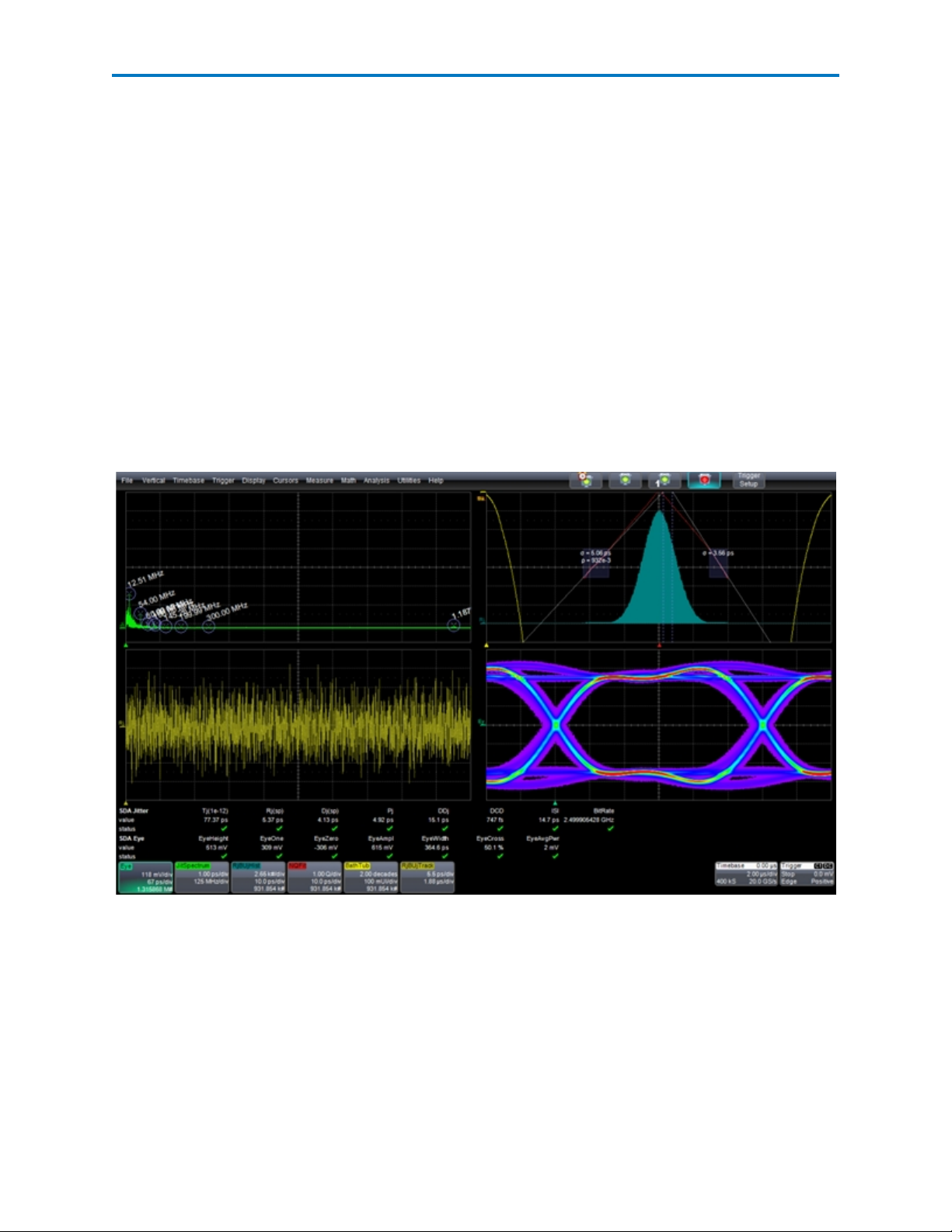
Quick View

The SDAIII-CompleteLinQQuick View shows the eye diagram, TIE track, bathtub curve, jitter histogram,
NQ-scale, and jitter spectrum (with peaks annotated) in a single, summarized view.

SDAII Quick View

You must specify only the input signal for analysis. You can also specify the crossing level.

12

921143 Rev A

Operator's Manual

Setting Up Quick View

Follow these steps to set up Quick View.

1. If you haven't done so already, touch Analysis → Serial Data on the menu bar or touch the Serial
Data Analyzer button on the Quick Access toolbar.

2. On the SDA Framework dialog, touch the Quick View button. The Signal Input(s) to be Analyzed
pop-up window opens.

3. On the Serial Data Input(s) section, if you are using a differential probe, touch the 1 Input (or Diff.
Probe) button. Now, touch inside the Data field below the 1 Input (or Diff. Probe) button and select
an input source from the Select Source pop-up window.

OR

If you are using two single-ended probes to calculate the differential signal, touch the Input1-Input2
button. Input2 is subtracted from Input1. Touch inside each Data field and select a source for each
Select Source pop-up window.

4. Increase the sampling rate of the signal by touching inside the Upsample by data entry field and
entering the upsample factor . at the bottom of the screen.

5. In the Crossing Level section, if you want to set an absolute crossing level, touch inside the Level is
field and choose Absolute from the pop-up menu. Then, touch inside the Abs Level data entry field
and enter the voltage level at which the signal timing is measured at the bottom of the window.

OR

If you want to use a relative level set to the selected percentage on each acquisition, touch inside the
Level is field and choose Percent from the pop-up menu. Then, touch inside the Percent Level data
entry field and enter the percentage . at the bottom of the window.

Note: You can touch the Find Level button to automatically find the level. The level is found by locat­ing the midpoint between the highest and lowest signal levels in the current acquisition.

6. Click OK to view the summary all on one screen.

Lane Configuration Process

SDAIII-CompleteLinQ offers many alternatives for configuring the analysis on up-to-four lanes, depending
on whether the oscilloscope is equipped with one of the "LinQ" options.

The main SDA Framework dialog is organized like a flowchart and shows some basic setup information
for the active lane, which is made active by touching/clicking one of the Lane selector buttons on the left
half of the dialog.

There are two main configuration approaches:

l Complete the entire configuration for a single lane, then proceed to the next

l Complete the configuration for all lanes at each box in the flow

921143 Rev A

13

SDAIII-CompleteLinQ Software

The minimum configuration requirement is to:

l Set up a signal

l Set up either a Reference Clock or Clock Recovery

If you have access to Eye Doctor II, you can optionally set up any Emphasis, Emulation/De-embedding of

fixtures, or Equalization you wish to apply to the lane before taking measurements.

You'll also want to set up the Eye, Jitter, Noise, and Crosstalk measurements to be used for analysis.

Return to the SDA Framework dialog at any time by touching/clicking the SDA tab.

Copying Configurations

An efficient approach is to complete the entire configuration for one lane then use the Copy Lane feature
on the SDA Framework dialog to copy that configuration to other lanes. You can then make unique set­tings by activating the desired Lane and touching the appropriate box in the flow to open the cor­responding configuration dialog.

Signal Input vs. Quick View

Signal configuration can be done either via the Signal Input dialog or the pop-up Quick View window.
However, any configurations already made on the Signal Input dialog will be replaced by configurations
made in the Quick View.

Synchronized vs. Independently Configurable Settings

Some settings will be synchronized across all lanes, either for simplicity or to ensure that it is straight­forward to compare results.

l Selections related to the display of results are synchronized across lanes—for example, wave-

forms, histograms, spectra and measurements. Waveforms and other plots for a given lane are
placed in a unique frame. See LaneScape Comparison Mode.

l Several other key settings are synchronized, including:

l Jitter Calculation Method (Jitter Parameters dialog)

l Eye Saturation (Eye Diagram dialog)

l Vertical Eye Scales (Eye dialog)

l Eye Style (Eye Diagram dialog)

l IsoBER start/stop/step (Eye Diagram dialog)

l log10BER (Jitter Parameters dialog)

l Repeating Pattern mode (Pattern Analysis dialog)

14

921143 Rev A

Operator's Manual

Signal Inputs

Set Up Signal

Follow these steps to define the characteristics of the input signal to be analyzed.

1. On the menu bar, touch Analysis → Serial Data to open the SDA Framework dialog. Then, touch the
Lane # button for the lane you wish to configure.

2. Touch the Signal Inputs button to open the Signal Inputs dialog.

3. In the Serial Data Input(s) section, if you are using a differential probe, touch the 1 Input (or Diff.
Probe) button.

Press the Input1 button and select an input source from the Select Source pop-up window.

OR

If you are using two single-ended probes to calculate the differential signal, touch the Input1-Input2
button. Input2 will be subtracted from Input1. Touch the Input1 and Input2 buttons and select a
source for each from the Select Source pop-up window.

4. If you want to increase the sampling rate of the signal, touch inside the Upsample by data entry field
and enter the upsample factor at the bottom of the screen.

5. In the Crossing Level section, if you want to set an absolute crossing level, touch inside the Level is
field and choose Absolute from the pop-up menu. Then, touch inside the Abs Level data entry field
and enter the voltage level at which the signal timing is measured . at the bottom of the screen.

OR

If you want to use a relative level set to the selected percentage on each acquisition, touch inside the
Level is field and choose Percent from the pop-up menu. Then, touch inside the Percent Level data
entry field and enter the percentage . at the bottom of the screen.

Note: You can touch the Find Level button to automatically find the level. The level is found by locat­ing the midpoint between the highest and lowest signal levels in the current acquisition.

6. Touch the Signal Type field and choose a standard signal type from the list. If you choose Custom
from the list of signal types, enter a bit rate in the Nominal Rate field.

921143 Rev A

15

SDAIII-CompleteLinQ Software

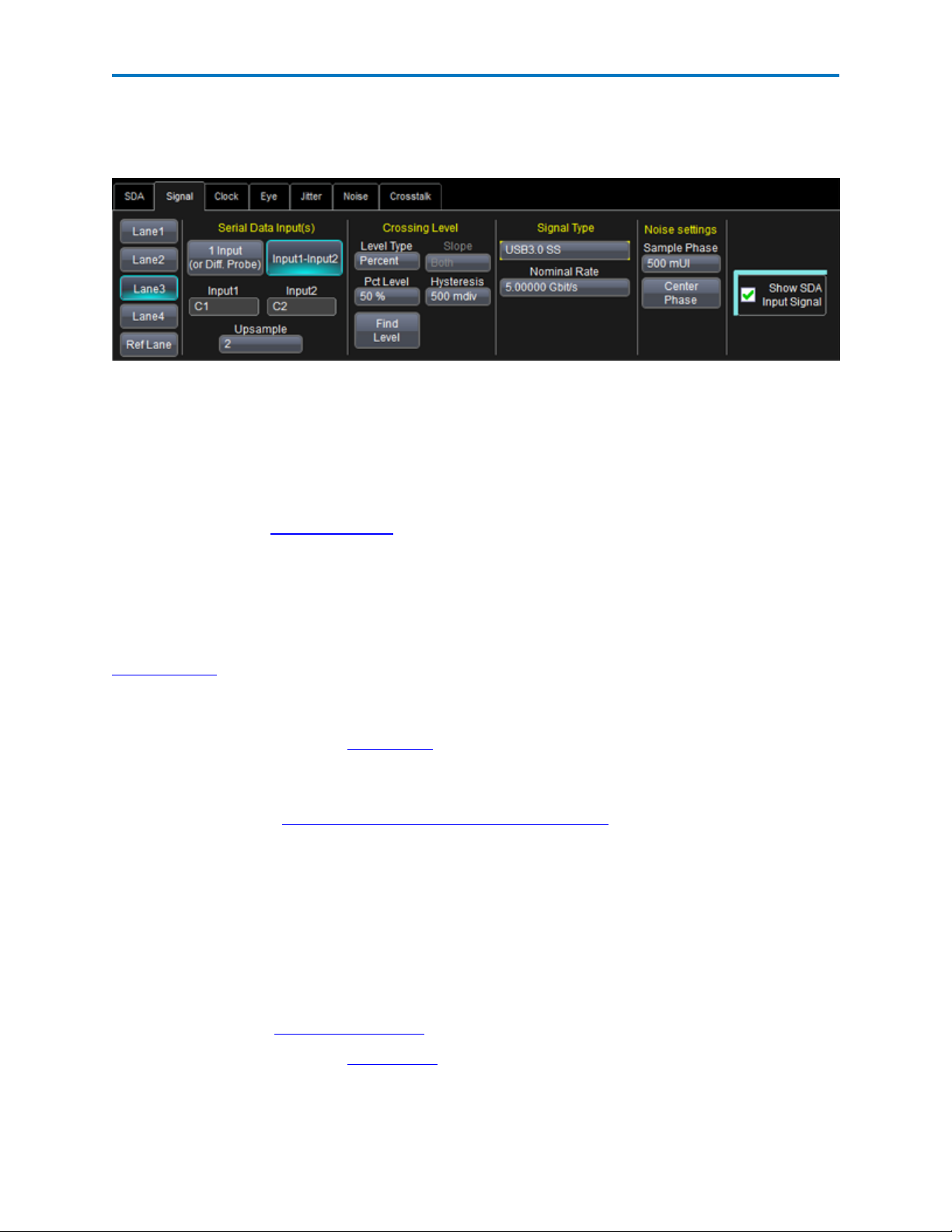
Signal Dialog

On the SDA Framework dialog, touch the Signal tab or the Signal Inputs button to access the Signal
dialog.

Lane 1-4 buttons at the far left let you select the Lane to be configured for signal. If you made this selec­tion earlier on the SDA Framework dialog, it will persist on the Signal dialog.

Serial Data Input(s) section lets you define the serial data input(s). If you are using a differential probe or
if your signal is connected by one coaxial cable, you can select 1 Input (or Diff. Probe) and specify the
input source in the Input1 box. If you are using two single-ended probes or two coaxial cables, you can
select Input1-Input2 and specify the input sources to use when calculating the differential signal. For
more information, see Serial Data Inputs.

Crossing Level section lets you to set the voltage level at which the signal timing is measured. The cross­ing level is set separately for the data and clock signals (if an external clock is selected) and can either be
an absolute voltage or a percentage of the signal amplitude via the relative selection. You can also con­figure a hysteresis level, and between positive, negative and both edge types for when the "Clock" Signal
Type is selected. The Crossing Level section on this dialog is for the data signal. For more information, see

Crossing Levels.

Signal Type section lets you choose a standard signal type. The signal type you choose automatically
sets the nominal bit rate for the selected standard, and populates the Mask Type selector in the Eye
dialog. For more information, see Signal Types.

Noise Settings includes settings that are used by the vertical noise measurements toolkit. Settings
include the Sample Phase, which determines where in the unit interval the sample is taken for the noise
measurement. Also, see How to Order SDAIII-CompleteLinQ Capabilities for information on which prod-
ucts include the vertical noise analysis capabilities.

NOTE:

l Many of the measurements in SDAIII-CompleteLinQrequire both a high sampling rate and long

memory to compute jitter and vertical noise accurately.

l Lower sampling rates can result in less accurate jitter measurements, and short record lengths can

give incomplete eye patterns or jitter and noise displays that diverge.

l For best results, acquire waveforms with at least 100,000 unit intervals, and of >100 iterations of

the pattern. See Jitter Pattern Analysis.

For step-by-step instructions, see Set Up Signal.

16

921143 Rev A

Operator's Manual

Serial Data Inputs

There are several scenarios for the configuration of the SeriaData Input(s) section.

If you are using a differential probe or if your signal is connected by one coaxial cable, use the 1 Input (or
Diff. Probe) button and select the input source.

If you have a differential signal transmitted on two two coaxial cables or two single-ended probes., use
the Input1-Input2 button and select the input channels used.

NOTE:There is no need to configure a math function to calculate the difference between to inputs. Doing
so adds additional computational steps, and unnecessarily uses RAM.

Lastly, any math function, memory trace, etc. can be used as an input, as well as any input channel.
When in Input1-Input2 mode, and when using traces that may have been the result of other processing
steps, be sure that both traces have the same record length and sample rate.

You can choose to upsample rate in the Serial Data Inputs dialog by a factor of two in order to provide a
higher sample density for analysis. In SDAII this was typically done to facilitate formation of eye diagrams
without gaps for bit rates integrally related to the sampling rate (for example, 20 GS/s is exactly eight
times 2.5 Gb/s), and especially for relatively short acquisitions. This, however, unnecessarily slowed
down the analysis process. When needing to upsample to remove gaps in the eye use the upsample con­trol in the Eye Diagram dialog.

Crossing Levels

The Crossing level section of the Signal dialog determines the voltage level where the arrival time of each
edge of the signal is measured. The crossing level is set separately for the data and clock (if an external
clock is selected).. The Crossing Level on this dialog is for the data. Setting the crossing level to a value
that is not optimal can result in higher than expected deterministic jitter, since the error in the timing of
the edges will be different for rising and falling edges.

The Level Type can be either absolute or relative.

The Absolute crossing level can be set directly in volts (or watts for an optical signal) , or you can click the
Find Level button to automatically find the level. The level is found by locating the midpoint between the
highest and lowest signal levels in the current acquisition. When you select the Absolute crossing level,
the crossing time used by both the jitter and eye pattern measurements is determined as the time at
which the signal level crosses the specified threshold. When Relative level is selected, the level is auto-
matically set on each acquisition. The value set is the selected percentage of the signal amplitude (which
equals base - top).

The Slope selector determines which edges are measured when "Clock" is selected in the Signal Type
selector in the Signal dialog.. The choices for slope are Pos(itive), Neg(ative) or Both Select the choice
that corresponds to the edge type that is used for clocking of the data in your device, or that is of inter­est in your analysis. For example, if you only latch data on positive edges, select Pos. If you clock on
both edges, you can select Pos or Neg rather than both in order to understand how the edge type affects
the jitter measurement.

The Hysteresis entry box sets the hysteresis level to use for edge detection, in units of vertical divisions.
The hysteresis is the vertical amount that the signal is required to travel beyond the crossing level to
allow detection of a crossing in the opposite direction. Incorporating hysteresis in the edge detection
algorithm prevents the software from finding false edges that would otherwise be detected due to noise

921143 Rev A

17

SDAIII-CompleteLinQ Software

or other small glitches in the signal. The default value is 500mdiv, or 1/2 a division. When the input sig­nals are properly scaled (i.e. to fill approximately 90% of the grid, vertically, this level of hysteresis should
be sufficient. When dealing with signals that result in closed eyes, a smaller value for hystersis may be
required.

More information about how the SDAanalysis software determines the edge timing using the crossing
level can be found in the Clock Recovery Theory section

NOTE: The Relative setting can potentially remove jitter by tracking slow level shifts between acqui­sitions, if this is not desired, use the Absolute level setting.

Signal Types

The signal type defines the compliance masks and bit rate for the selected standard.

When you touch the Signal Type field, a pop-up table of standard signal types is shown. Touch the
desired signal type to populate the Signal Type field. The list of signal types is taken from the SDAMask
Database. As new serial data standards are invented, masks are added to the database.

The Nominal Rate entry box in the Signal dialog is automatically populated when selecting a signal type
other than custom.

When choosing Custom from the Signal Type pop-up menu, always enter a bit rate in the Nominal Rate
entry box. Using an incorrect Nominal Rate can lead to incorrect equalizer results, since this value is used
by several of the equalizers that are available the oscilloscope includes Eye Doctor II functionality. The
Custom selection does not specify any eye masks, and the Mask Type selector in the Eye dialog will be
greyed out.

18

921143 Rev A

Operator's Manual

Clock

Set Up Clock Recovery

Follow these steps to define the clock recovery method to be used for a given input signal.

1. Touch Analysis → Serial Data on the menu bar.

2. On the SDA Framework dialog, touch the Clock Recovery button.

3. In the Data or Bit Rate section, touch inside the Bit Rate field and enter a bit rate, or use the pop-up
keypad to enter a specific value. .

Note: Alternatively, touch the Find Bit Rate button to automatically find the expected bit rate.

4. Optionally, and when using an explicit reference clock, go to the Reference Clock section, touch Des-
kew and set the deskew value using either the keypad or the WaveScan knob. The Deskew control
shifts the clock edges relative to the data signal v

5. In the PLL Setup... section, check the PLL On box (enabling the function).

6. Touch PLL Type and select the type of PLL to be used in the clock recovery function. The choices are
at least FC Golden and Custom. Other choices which may be enabled depending on the signal type
selected are: PCI-Express Gen1, PCI-Express G2 A 3dBpk 16 MHz fc, PCI-Express G2 B 3dBpk 8 MHz
fc, PCI-Express G2 C 1dBpk 5 MHz fc, DVI, USB, and FB-DIMM.

Clock Recovery Dialog

An accurate reference clock is central to any jitter measurement, including all the measurements per­formed by SDAIII-CompleteLinQ. The recovered clock is defined by the times at which the specified signal
(either data or reference clock) crosses the specified threshold. Starting with zero, the clock edges are
computed at specific time intervals relative to each other. A 2.5 GHz clock, for example, will have edges
separated in time by 400 ps.

On the SDA Framework dialog, touch the Clock tab or the Clock Recovery button to access the Clock
dialog.

Lane 1-4 buttons (far left) - Let you select the Lane to be configured. If you made this selection earlier on
the SDA Framework dialog, it will persist on the Clock dialog.

Data or Bit Rate section - Lets you define a custom expected bit rate, or you can click the Find Rate Now
button to automatically find the bit rate from the signal. If you do neither, this field remains set to the
standard's nominal bit rate. . When checked, Find Rate Every Sweep treats each sweep independently.

921143 Rev A

19

SDAIII-CompleteLinQ Software

With each acquisition, the clock recovery algorithm determines the optimal recovered clock. Using this
setting causes statistics to be reset with every sweep, including the population within eye diagrams.

Reference Clock section - Enables positioning of the clock edges relative to the data signal. It shifts the
clock signal relative to the data signal. For convenience, it duplicates controls found elsewhere: the Use
Explicit Clock Ref checkbox (serving the same function as the multiplexer switch on the SDA Framework
dialog) and the Slope, Deskew, and Multiplier fields (also found on the Ref. Clock dialog). The Slope set­ting (active when using an explicit reference clock) determines whether to use positive, negative, or both
edges of the clock signal as the edges that define the system clocking. Deskew allows you to fine-tune the
skew between the clock and data. Varying the deskew value will have the effect of shifting the eye dia­gram. .

PLL Setup... section - Sets the type and bandwidth of the digital PLL used in SDAII measurements. The
PLL bandwidth limits the response of the recovered clock to high rate variations in the data rate. For
example,depending on the type of PLL, a PLL bandwidth of 5 MHz will allow the recovered clock to track
frequency variations below approximately half this rate, thereby removing their effect from jitter and eye
pattern measurements. Configure this section to match the behavior of the receiver's PLL.

For step-by-step instructions, see Set Up Clock Recovery.

PLL Setup

The PLL Setup section of the Clock dialog contains the controls to set the type and bandwidth of the dig­ital PLL used in all SDAIII-CompleteLinQ measurements. The PLL bandwidth limits the response of the
recovered clock to high rate variations in the data rate. Configure this section to match the behavior of
your receiver's PLL.

Example: A PLL bandwidth of 5 MHz allows the recovered clock to track frequency variations below
approximately half the frequency, therefore removing the effect from jitter and eye pattern meas­urements. The software PLL implemented in SDAIII-CompleteLinQ allows you to choose among several
types of PLL.

The selected PLL is applied to either the data stream under test or the selected clock source (if a Ref­erence Clock is in use) when the PLL On control is checked. The PLL recovers a reference clock from the
selected source, which is used by all subsequent SDAIII-CompleteLinQ measurements.

BW indep of Data

When this option is checked, the PLL algorithm will keep track of the "local" transition density by tracking
the number of UI between edges, and use this information in addition to the last edge's phase difference
in determining the amount of error to feedback into the control loop. This allows the clock recovery algo­rithm to track the underlying clock when in the presence of varying transition densities. The result is that
the PLL will implement the configured PLL bandwidth, even if the local transition density varies sig­nificantly from its average value. Use this setting when you want the clock recovery to model a receiver
that uses a PLL which compensates for varying transition density.

20

921143 Rev A

Operator's Manual

PLLTypes

FC GOLDEN

FC Golden is the default selection and implements the golden PLL as defined in the Fibrechannel spec­ification. By default, the golden PLL is set to a cutoff frequency of 1/1667 times the bit rate of the signal
under test. This ratio can be adjusted from 1/10 to 1/1e6.

Make the following settings for the FC Golden PLL on the Golden PLL dialog at the far right of the screen:

l Touch inside the Cutoff Divisorfield and enter a value using the pop-up keypad. The default value

of 1667 is the industry standard for a Golden PLL and equals the ratio of the Bit Rate to the PLL Cut­off frequency.

The PLL cutoff divisor is the value by which the bit rate is divided to compute the cutoff frequency
for the loop bandwidth of the clock recovery operation for sequential eye pattern, jitter, and bit
error rate functions. This control is variable from 10 to 1,000. A low PLL cutoff divisor means the
PLL tracks and, therefore, attenuates jitter at higher frequencies.The default value of 1667 causes
the clock recovery to operate as a golden PLL, as defined in the Fibrechannel specification.

l The PLL Cutoff frequency control reads the frequency corresponding to the Cutoff Divisor. Alter-

natively, the PLL Cutoff frequency may be provided and the nearest cutoff divisor is then com­puted from the entry.

PCI-EXPRESS

There are four PCI-Express selections that meet the following standards:

l PCI-Express Gen1

l PCI-Express Gen2 A

l PCI-Express Gen2 B

l PCI-Express Gen2 C

DVI

921143 Rev A

21

SDAIII-CompleteLinQ Software

The DVI selection displays the DVIPLL dialog at the far right of the screen and follows the requirements
of the DVI (Digital Video Interactive) and HDMI (High Definition Multimedia Interface) specifications.
These specifications call out a clock recovery function having a single-pole PLL loop response with a cutoff
of 4 MHz.

FB-DIMM

The FB-DIMM selection applies a filter that replicates Fully-buffered DIMM.

USB

The USB selection applies a filter that meets the USB 3.0 SS requirements.

CUSTOM

The Custom selection shows the Custom PLL dialog on the far right of the screen and allows you to select
either a first or second order loop response. The first order response allows you to select a pole
frequency that sets the PLL cutoff, and a zero frequency that must be higher than the pole frequency
that limits the stop-band attenuation.

The second order PLL allows you to select the natural frequency and damping factor. The damping factor
determines the transient behavior of the phase locked loop and is variable from 2 to 0.5.

l A damping factor above 0.707 results in an under-damped response and the PLL is over-corrected

to a sudden change in frequency; however, reacts quicker to the change.

l A damping factor below 0.707 provides an under-damped response that reacts more slowly to sud-

den changes in frequency; however, does not over-correct.

The default value of 0.707 represents a critically damped response that provides the fastest reaction time
without over-correcting.

The second order PLL with a damping factor of 0.707 is specified in the serial ATA generation II document.
This type of PLL is also very useful for measuring signals with spread-spectrum clocking because it can
accurately track and remove the low-frequency clock spreading while allowing the signal jitter to be meas­ured. The natural frequency is somewhat lower than the actual 3 dB cutoff frequency given by the equa­tion:

The quantity is the damping factor, and is the natural frequency. For a damping factor of 0.707,

22

921143 Rev A

Operator's Manual

this relationship is fc= 2.06 fn. Settings for the Custom PLL: Touch inside the Poles field to select the
order of the PLL. The number of poles can be 1 or 2.

Clock Recovery Theory

Eye, jitter and vertical noise analysis all require a clock that defines the boundaries of each unit interval.
Additionally, the clock is used to determine the difference between actual and expected arrival times of
data edges (i.e., the time interval error, or TIE measurements). In many of today's high-speed serial stand­ards, the clock is not a physical signal but is instead derived from the data signal via clock recovery hard­ware or software. SDAIII-CompleteLinQ includes a clock recovery algorithm that determines the clock
from the either the data signal or from an explicit clock signal.

You may use a PLL as part of the clock recovery algorithm in order to best emulate the PLL in a receiver.
The recovered clock is defined by a list of times that correspond to expected edge arrival times.

The first step in creating a clock signal that is tracked by a PLL is to create a digital phase detector. This is
simply a software component that measures the location in time when a signal crosses a given threshold
value. Even given the maximum sampling rate available), interpolation is necessary in order to accurately
determine crossing times. Interpolation is automatically performed by SDAIII-CompleteLinQ. Inter­polation is not performed on the entire waveform; rather, only the points surrounding the crossing level
are interpolated. A cubic interpolation is used, followed by a linear fit to the interpolated data to find the
precise time that a data signal edge traverses the crossing level (see figure below).

SDA Edge Time Determination

Clock recovery implementation in the SDA is shown in the following figure. This algorithm generates time
values corresponding to a clock at the data rate. The computation follows variations in the data stream
being tested through the use of a feedback control loop correcting each period of the clock by adding a
portion of the error between the recovered clock edge and the nearest data edge.

921143 Rev A

23

SDAIII-CompleteLinQ Software

Clock Recovery Implementation Usinga PLL

As shown in the previous image, the initial output and the output of the digital phase detector are set to
zero. The next time value output is equal to the nominal data rate. This value is fed back to the com­parator on the far left which compares this time value to the measured time of the next data edge from
the digital phase detector. The difference is the error between the data rate and the recovered clock, and
can also incorporate the measurement of the number of UI's since the last edge(that is, the local tran­sition density).This difference is filtered and added to the initial base period to then generate the cor­rected clock period. The filter controls the rate of this correction by scaling the amount of error fed back
to the clock period computation. The choice of filter in SDAII and SDAIII-CompleteLinQ includes a single­pole infinite impulse response (IIR) low-pass filter (the golden PLL, as defined by FibreChannel), a 1 pole 1
zero filter, and a 2 pole 1 zero filter. The equation of the golden PLL 1 pole filter is:

The value of ykis the correction value for the kthiteration of the computation and xkis the error
between the kthdata edge and the corresponding clock edge. Notice that the current correction factor is
equal to the weighted sum of the current error and all previous correction values. The multiplier value is
set to one in the SDA, and the value of n is the PLL cutoff divisor set from the Golden PLL dialog. The cut­off frequency is Fd/n, where Fd is the data rate. This filter is related to its analog counterpart through a
design process known as impulse invariance and is only valid for cutoff frequencies much less than the
data rate. For this reason, the minimum PLL cutoff divisor setting is 20 in the SDA.

The factor n determines the number of previous values of the correction value y used in the computation
of the current correction value. This is theoretically infinite; however, there is a practical limit to the
number of past values included.

Set Up Reference Clock

An accurate reference clock is central to the measurements performed by SDAIII-CompleteLinQ. When
the clock is recovered from data, the clock is defined from the locations of the data's crossing points in
time. When a reference clock is used, the clock is defined from the locations of the reference clock's cross­ing points. Starting with zero, the clock edges are computed at specific time intervals relative to each
other.

Example: A 2.5 GHz clock has edges separated in time by 400 ps. Making a 2.5 GHz clock from a 100 MHz
reference clock requires setting the Multiplier to 25.

Follow these steps to define the crossing points.

24

921143 Rev A

Operator's Manual

1. Touch the Ref. Clock Input button on the SDA Framework dialog to access the Ref. Clock dialog. If
the Ref. Clock Input button is disabled, touch the multiplex button next to the Clock Recovery but­ton to enable the Ref. Clock Input button.

2. If not already active, touch the Lane # button to activate the lane for which you're configuring the ref­erence clock.

3. If using a single source or a differential probe, touch the 1 Input button, then touch the Input1 field
and from the Select Source window choose the channel that is the source for this input.

OR

If using two sources, touch the Input1-Input2 button, then touch the Input1 field and from the
Select Source window choose the channel that is the source for the first input. Repeat for the Input2
field.

4. To increase the sampling rate of the signal, touch the Upsample by field and enter the upsample fac­tor.

5. To set a crossing level, touch Level Type and chose either Absolute or Percent (relative).

If Percent, touch the Pct Level field and enter the percent (voltage level) between base at top at
which to measure signal timing.

OR

If Absolute, touch the Abs Level field and enter the voltage level at which the signal timing is meas­ured.

You can make your entries using either the pop-up keypad or the WaveScan knob.

NOTE: Alternatively, you can touch the Find Level button to automatically find the level. The level is
found by locating the midpoint between the highest and lowest signal levels in the current acqui­sition.

6. Touch the Clock Slope field and choose Positive, Negative, or Both to use positive, negative or both
edges of the clock signal as the edges that define the system clocking.

7. To fine-tune the skew between the clock and the data, touch the Deskew field and use the pop-up
keypad or theWaveScan knob to enter a value.

8. To upsample the reference clock signal, touch the Clock Multiplier field and enter a value.

921143 Rev A

25

SDAIII-CompleteLinQ Software

Eye Measurements

Eye Measurements Overview

Eye diagrams are a key component of serial data analysis. They are used both quantitatively and qual­itatively to understand the quality of the signal communications path. Signal integrity effects such as
intersymbol interference, loss, crosstalk and EMIcan be identified by viewing eye diagrams, such that
the eye is typically viewed prior to performing any further analysis. SDAIII-CompleteLinQ includes the
capability to display eye diagrams of up-to-four lanes plus a reference lanes simultaneously.

Eye diagrams can be built using either a single sweep or over multiple sweeps.

NOTE: To accumulate an eye over multiple sweeps, you should have the Find Rate Every Sweep check­box (on the Clockdialog) unchecked.

The descriptor box for an Eye diagram includes following information:

l Top line: volts/division of the eye

l Second line: time/division of the eye

l Third line: the number of unit intervals (UI)in the eye

If cursors are enabled, cursor values appear in subsequent lines.

The main dialog for eye measurements is accessible by clicking the Eye Meas button on the SDAIII-Com­pleteLinQ dialog, or by selecting the Eye tab.

Eye Measurements includes eye diagrams, mask tests and parameters calculated from eye diagrams.

26

921143 Rev A

Operator's Manual

Eye Dialog

The Eye dialog is the principal tool for setting up Eye diagrams. Click the Eye Meas. button on the SDA
Framework dialog to access the Eye dialog.

The Eye Modes section in the Eye dialog lets you choose an eye mode, either Single Eye, Dual Eye
Trans/Non-trans.

The Masks section in the Eye dialog lets you select different modes for the selected standard. A standard
may define different masks for different measurement types. The Mask Margin lets you define how
much to enlarge the mask, to make sure that your signal passes the mask plus margin.

Set Up Eye Diagram

Follow these steps to define the type, shape, and size of an Eye diagram.

1. Open the Eye dialog.

2. Place a checkmark in the Enable Eye Meas. checkbox to turn on eye measurements.

3. If you want to turn off the eye parameters display, touch the Turn Off Eye Params. button.

4. In the Eye Mode section, touch the Mode field and choose an eye mode from the pop-up menu.

5. Touch the Vertical Auto Fit checkbox if you want to scale the eye pattern. These controls are dis­abled (grayed out) if the mask is specified in absolute units (volts and seconds); that is, if the stand­ard does not allow auto fit.

The vertical auto fit function sets the scaling of the eye pattern so that the one level is at the second
vertical division above center, and the zero level is at the second division below center. The Vertical

Auto fit checkbox is automatically checked or unchecked depending on the selected Signal Type.

Example: When an absolute mask like XAUI is selected, the Vertical Auto fit checkbox is unchecked;

however, it is checked for a normalized mask like FC1063.

Scaling for absolute mask signals is accomplished by setting the vertical scale of the input signal.

6. In the Mask section, touch the Mask Type field and choose a mask type from the pop-up menu.

7. Touch inside the X field and enter a value from 0 to 100%. As you enlarge the mask's margin, you
lengthen the horizontal dimension, bringing the mask closer to the crossing points of your eye dia­gram. This reduces the amount of jitter that can still pass the eye.

921143 Rev A

27

SDAIII-CompleteLinQ Software

8. Touch inside the Y field and enter a value from 0 to 100%. As you enlarge the mask's Y margin, you
widen the vertical dimension, bringing the mask closer to the top and bottom of your eye diagram.
This reduces the amount of vertical eye closure that can still pass the eye.

9. Margin only center area checkbox - Check to have only the center hexagon or diamond expand
when the mask margin is set to a value other than 0%

10. Vertical Eye Scales selectors - Select a mode of operation for vertical scaling the eye. Eyes for all ena-

bled lanes will use the same setting.

l Normal: Select to have the volts/div of the Eye trace for each lane follow the vertical scale of

the signal input to the Eye diagram algorithm. This typically will be the volts/div of the source
channel when using 1 input, or the sum when using two inputs.

l Auto Fit All Lanes: Select to adjust the vertical scales to a value and offset that places the "1"

level at +2.5div, and the "0" level at -2.5div.

l Lock All Lanes:Select to set the vertical scales to the value entered in the adjacent Ver Scale

entry box

Eye Diagram Configuration Dialog

The Eye Diagram right-hand dialog lets you configure how the eye diagram is displayed.

Show Eye - Displays the eye diagram(s).

Show Mask- Displays the mask template(s). If Custom or Clock is chosen for the Signal Type in the Signal

tab, then this checkbox is greyed out. (Users can create custom masks by defining a new signal type.)

Show IsoBER - Displays IsoBER, which provides a visual representation of the extrapolated eye diagram.
The IsoBER is calculated using the same algorithm that is used for the Crosstalk Eye.

Eye Saturation- Use the slider to increase or decrease eye saturation. The setting for saturation adjusts
the color grading or intensity. Slide to the left to reduce the threshold required to reach saturation.

Show Failures- Place a checkmark to show the mask failures. Mask failures are identified by contrasting
color spots which appear anywhere the data intersects the mask template. If Custom or Clock is chosen
for the Signal Type in the Signal tab, then this checkbox is greyed out.

Eye Style- You can choose the style you want to use to display the eye diagram. The selections are color­graded or analog persistence. In color-graded persistence, pixels are given a color based on the pixel's rel­ative population and the selected Eye Saturation. The color palette ranges from violet to red. When
analog persistence, is selected, the color used mimicks the relative intensity that would be seen on an
analog oscilloscope.

28

921143 Rev A

Operator's Manual

IsoBERfrom/to/step - Select the range of BER values for which you would like to show contours in the
ISOBer plot.

Upsample- Increase from 1 to a higher number (e.g. 5) to fill in gaps in the eye diagram. Gaps can occur
when the bitrate is extremely close to a submultiple of the sampling rate, such that the sampling of the
waveform does not move throughout the entire unit interval. Gaps can also occur when using a record
length that does not sample a sufficiently large number of unit intervals. (Using record lengths of >= 1 mil­lion points is recommended in order to acquire tens of thousands, if not hundreds of thousands, of unit
intervals.)

Eye diagam with ISOBer superimposed

Eye Modes

There are two eye modes you can choose when setting up an eye measurement:

Single Eye- This mode overlays all the UIs from all acquisitions.

Dual Eye Transition/Non-Transition - Divides the signal's UIs into two separate eyes: ones comprised of

UIs starting with a transition and one comprised of UIs without. The PCIe standard refers to these as Tran­sition and Non-Transition eyes. This display mode is useful for those serial data standards using mask
testing for both types of eyes (PCI Express and FB-DIMM Point-to-Point).

Mask Testing

Mask testing to either absolute or normalized masks can be performed with SDAIII-CompleteLinQ. You
can determine where the signal has violated the mask, how many failures have occurred, and determine
which particular UI is in violation.

921143 Rev A

29

SDAIII-CompleteLinQ Software

When selecting a Signal Type on the Signal tab for a serial data standard, the Mask section of the Eye
Measure. Each standard has a set of required tests; some of the standards specify using a specific mask

template. Masks templates are stored in the database file EyeMaskProps.mdf, which can be edited via
the Mask Database Editor tool. A shortcut to launch this tool can be found in the LeCroy folder of the
Start menu.

Masks are either "absolute" or "normalized". Absolute masks specify specific voltage and time values.
When using absolute masks, the position of mask features will depend on the volts/div setting of the
mask. Normalized masks reference grid locations rather than absolute voltages.

You can also define how much to enlarge the mask in order to ensure your signal passes the mask plus
some additional margin.

Mask Margin

The Mask Margin setting lets you increase or decrease the size of an Eye mask.

1. Touch inside the X field and enter a value from 0 to 100%. As you enlarge the mask's X margin, you
lengthen the horizontal dimension, bringing the mask closer to your waveform. Consequently, you
will have more failures.

2. Touch inside the Y field and enter a value from 0 to 100%. As you enlarge the mask's Y margin, you
widen the vertical dimension, bringing the mask closer to your waveform. Consequently, you will
have more failures.

3. Touch the Vertical Auto fit checkbox if you want to scale the eye pattern.

Note: The vertical autofit function sets the scaling of the eye pattern so that the one level is at the second
vertical division above center, and the zero level is at the second division below center. The Vertical Auto
fit checkbox is automatically checked or unchecked depending on the Signal Type that you selected. For
example, when an absolute mask like XAUI is selected, the Vertical Auto fit box is unchecked; but, it is
checked for a normalized mask like FC1063.

Scaling for absolute mask signals is accomplished by setting the vertical scale of the input signal.

30

921143 Rev A

Operator's Manual

Eye Parameters Dialog

The Eye Parameters right-hand dialog lets you choose which parameters you want to show on the
screen. You can also enter a slice width. The slice width is a percentage of the duration of a single bit (the
part of the pattern over which the extinction ratio is measured). Setting a percentage value indicates how
much of the central portion of the bit width to use.

Both the Jitter Measurements and the Eye Parameters can be on at the same time. They are shown sep­arately on the table display. To turn off all eye parameter measurements, touch the "Turn off Eye
Params"button located on the left side of the adjacent Eye Diagram dialog.

Note: The oscilloscope's Measure table can also be displayed.

Eye Measurement Parameters

There are several important measurements are made on eye patterns. Many standards specify them as
part of required tests. Eye measurements mainly deal with amplitude and timing (outlined later in this
section). For information on setting up eye measurements, see Set Up Eye Diagram.

Eye Amplitude

Eye amplitude is a measure of the amplitude of the data signal. The measurement is made using the dis­tribution of amplitude values in a region near the center of the eye (the "slice width")selected by the user
(normally 20% of the distance between the zero crossing times). The simple mean of the distribution
around the 0 level is subtracted from the mean of the distribution around the 1 level. This difference is
expressed in units of the signal amplitude (normally voltage). This measurement algorithm is best suited
to eye diagrams that are rendered from optical rather than electrical signals. In the presence of inter-sym­bol interference and/or equalization, it may not give reasonable results.

One Level

Simple mean of the 1 or high state of the eye within the selected slice width

Zero level

Simple mean of the 0 or low state of the eye within the selected slice width.

Eye Height

The eye height is a measure of the signal-to-noise ratio of a signal. The mean of the 0 level is subtracted
from the mean of the 1 level as in the eye amplitude measurement. This number is modified by sub­tracting three times the standard deviation of both the 1 and 0 levels. The measurement provides an indi­cation of the eye opening and is made on the central region (normally 20%, user changeable) of the UI
(bit period). This measurement algorithm is best suited to eye diagrams that are rendered from optical

921143 Rev A

31

SDAIII-CompleteLinQ Software

rather than electrical signals. In the presence of inter-symbol interference and/or equalization,it may not
give reasonable results.

Eye Width

This measurement gives an indication of the total jitter in the signal. The time between the crossing
points is computed by measuring the mean of the histograms at the two 0 crossings in the signal. Three
times the standard deviation of each distribution is subtracted from the difference between these two
means. This measurement algorithm is best suited to eye diagrams that are rendered from optical rather
than electrical signals. In the presence of inter-symbol interference and/or equalization, it may not give
reasonable results.

Extinction Ratio

This measurement, defined only for optical signals, is the ratio of the optical power when the laser is in
the ON state to that of the laser in the OFF state. Laser transmitters are never completely shut off since a
relatively long period of time is required to turn the laser back on (therefore limiting the rate at which the
laser can operate). The extinction ratio is the ratio of two power levels (one very near zero) and its accu­racy is greatly affected by any offset in the input of the measurement system. Optical signals are meas­ured using optical-to-electrical converters on the front end of the SDA. Any DC offset in the O/E must be
removed prior to measurement of the extinction ratio. This procedure is known as dark calibration. The
output of the O/E is measured with no signal attached (also referred to as being dark) and this value is
subtracted from all subsequent measurements.

Eye Crossing

Eye crossing is the point where the transitions from 0 to 1 and from 1 to 0 reach the same amplitude. This
is the point on the eye diagram where the rising and falling edges intersect. The eye crossing is expressed
as a percentage of the total eye amplitude. The eye crossing level is measured by finding the minimum
histogram width of a slice taken across the eye diagram in the horizontal direction (as the vertical dis­placement of this slice is varied).

Average Power

The average power is a measure of the mean value of the signal, derived from all levels contained within
the eye diagram. It can be viewed as the mean of a histogram of a vertical slice through the waveform
covering an entire bit interval. Unlike the eye amplitude measurement where the 1 and 0 histograms are
separated, the average power is the mean of both histograms combined. Depending on the data coding
used, the average power can be affected by the data pattern. A higher density of 1s, for example, results
in a higher average power. Most coding schemes are designed to maintain an even 1s density resulting in
an average power that is 50% of the overall eye amplitude.

Eye BER

Eye BER is an estimate of the bit error ratio is made from the eye diagram. It is derived from a meas­urement of the Q-factor, as described below.

32

921143 Rev A

Operator's Manual

This measurement algorithm is best suited to eye diagrams that are rendered from optical rather than
electrical signals. In the presence of inter-symbol interference and/or equalization, it may not give rea­sonable results.

The Q factor is a measure of the overall signal-to-noise ratio of the data signal. It is computed by taking
the eye amplitude (the difference between the mean values of the 1 and 0 levels) and dividing it by the
sum of the noise values (standard deviations of the 1 and 0 levels).

All of these measurements are taken in the center (usually 20%) of the eye. Users can show the Q factor
via the Measure system.

Mask Hits

Number of samples where the signal impedes the mask.

Mask Out

Number of samples where the signal does not impeded the mask.

921143 Rev A

33

SDAIII-CompleteLinQ Software

Eye Analysis Theory

Eye diagrams are persistence maps, where each pixel in the map takes on a color that indicates how
frequently a signal has passed through the time (within a UI) and voltage specified for that pixel. Theeye
diagram shows all values a digital signal takes on during a bit period. A bit period (or UI) is defined by the
data clock, so some sort of data clock is needed to measure the eye pattern.

Eye Diagram

Eye Diagramming in Older Oscilloscopes

The "traditional" method of generating an eye pattern that was used before oscilloscopes had the ability
to determine an eye from a single sweep involved building a persistance map over many sweeps. Signals
were acquired using the data clock as a trigger. One or more samples taken on each trigger were stored
in a persistence map with the vertical dimension equal to the signal level, with the horizontal position
equal to the sample position relative to the trigger. The eye pattern filled in after a large number of mul­tiple occurrences of time and amplitude values (counted by incrementing counters in each x,y bin) for all
the data points collected. Users would typically put the trigger point "off screen", and build the per­sistance map until it showed sufficient data.

Timing jitter is indicated by the horizontal distribution of the points around the data crossings. The his­togram of the bins around the crossing points provides the distribution of jitter amplitude. This tra­ditional method, unfortunately, includes the oscilloscope's trigger jitter, with the consequence that the
jitter seen in the eye diagram was not just the jitter in the signal itself.

A recovered clock is used if there is no access to a data clock. In the traditional method, the recovered
clock is normally a hardware PLL designed to operate at specific data rates and with a cutoff frequency of
Fd/1667. A drawback of a hardware clock recovery circuit is that jitter associated with its trigger circuit
adds to the measured jitter by creating uncertainty in the horizontal positioning of the eye pattern sam­ples. Another drawback is that the clock recovery PLL is not likely to be controllable, and may not meet
the exact requirements for a specific standard.

34

921143 Rev A

Operator's Manual

Eye Patterns

SDAIII-CompleteLinQmeasures eye patterns without using a trigger. This is done using the software clock
recovery (discussed in Set Up Clock Recovery) to divide the data record into segments along the time
values of the clock. For the purpose of dividing the time line into segments, the time resolution is essen­tially infinite. The samples occur at fixed intervals of 25 or 50 ps/pt (for 40 or 20 GS/s sampling rate). The
samples are positioned relative to the recovered clock edge times, and the segments delimited by the
clock (the unit intervals or bits) are overlayed by aligning the clock delimited boundaries.. A monochrome
or color persistence display is used to show the distribution of the eye pattern data. Since the unit inteval
are determined from the recovered clock and not from the oscilloscope's trigger position, this method
does not include jitter from any trigger circuit.

921143 Rev A

35

SDAIII-CompleteLinQ Software

Jitter Measurements

Set Up Jitter Measurements

Touch the Setup Jitter Measurements button on the Serial Data Analysis II dialog to access the Jitter
Measure dialog. The SDAII jitter analysis follows a flow of events.

The main Jitter Measure dialog shows the basic flow of the jitter analysis through a simple block diagram
progressing from left to right. Each block in the diagram is also a button. Touching any of the buttons
opens its corresponding right hand dialog.

Jitter Measurements flow diagram dialog

SDAII jitter analysis techniques are described in the following topics. The main parts of this flow cor­respond to the block diagram on the main Jitter Measure dialog.

A comprehensive white paper describing how jitter is measured, SDAIII Jitter Calculation Methods, on
the Teledyne LeCroy website.

Enable Jitter Measure

If this checkbox is unchecked, it turns off all traces and parameters. However, the setup remains in effect.
When checked, the traces and parameters remain unchanged.

TIE Trend

NOTE:There is no block or button for TIE Trend on the dialog. However, the TIEtrend is calculated in the
background.

First, the TIE trend is calculated, which is the deviation of each edge from the ideal provided by the recov­ered clock. See Set Up Clock Recovery.

Jitter Filter

1. The TIE trend, which only has a sample for each edge in the input waveform, is converted to what we
call a track or TIETrack, which is uniformly sampled at every UI, by inserting interpolated samples for
each UI where there was no edge (virtual edge). The track is also given a time axis. The TIE can now be
filtered.

2. This step allows a bandpass filter be applied to the TIETrack. Use the Filter Mode to turn the function
On or Off. You can specify a Low Pass Cutoff, High Pass Cutoff, and a Transition Width.

3. Any Jitter filtered from the Jitter Track at this point is not passed on to any of the downstream anal­ysis.

36

921143 Rev A

Operator's Manual

Pattern Analysis

A progress bar and helper information is displayed under the Pattern Analysis button, and an LEDabove
to inform the user the status of the pattern analysis.

1. First the data pattern is found.

2. Then, a DDj analysis is performed on the TIE trend. The average TIE is calculated for each DDj class.
The DDj classes can be defined either by where the edge occurs in a repetitive pattern or by the N-bit
sequence occurring prior to the edge.

3. From this analysis, a list of DDj values and populations is created for each classification made from
step 1.

4. From this analysis, the following are calculated:

l DDj histogram

l DDj plot

l DDj parameter

l DCD (Duty Cycle Distortion ) parameter

l ISI parameters

5. The DDj is removed from each edge in the TIE Trend (according to their classification from step 1) to
create an RjBUj TIE Trend (RjBUjTrend), a TIE sequence (in which the DDj is removed, but still con­tains all the (Rj) Random jitter, and the (BUj) Bounded-Uncorrelated jitter). The most common case
of BUj is periodic jitter, where the period is unrelated to the data rate.

Jitter Track

1. In this step, the RjBUjTrend is converted to a track (RjBUjTrack) by inserting interpolated samples
into the RjBUj Trend for each UI where there was no edge, thereby yielding a uniformly sampled TIE
waveform with a sample for every UI and a time axis.

2. This function provides the capability to show/hide the RjBUjTrack, the TIETrack, and the PLLTrack.

The PLLTrack shows the jitter tracked out by the PLL compared to an ideal clock of frequency (found
by the Find Bit Rate function).

Jitter Spectrum

1. The spectral analysis step takes the FFT of the RjBUjTrack (DDj removed). Notice how the Jitter Spec­trum is showing magnitude. Therefore, to get peak-to-peak jitter you must multiply by 2.

2. The background of the spectrum is estimated and integrated to get a spectrally derived Random
jitter, Rj(sp). If the jitter model selected in the Jitter Params dialog is Dual-Dirac Spectral, then this is
the Rj used in the jitter breakdown.

3. The peaks in the spectrum are identified and used for further periodic jitter analysis.

4. A version of the spectrum is created which only keeps the peaks above the threshold.

5. The inverse FFT (PjInvFFT) of the peaks only spectrum is created. The peak-to-peak Pj is measured
from this waveform.

921143 Rev A

37

SDAIII-CompleteLinQ Software

Jitter Histogram

Update the TIE histogram and the Rj+BUj histogram with the values in the TIETrend and the RjBUjTrend,
respectively. For multiple input waveforms, the histogram continues to accumulate until the Clear
Sweeps Front Panel button is pressed.

Jitter Parameters

The fit extrapolation for the NQ-scale model can be shown on the histogram for the NQ-scale model.

The Rj+BUj jitter distribution with the analytical tail extrapolations is then convolved with the DDj dis­tribution (found during the Pattern Analysis Step) to create the total jitter distribution. This is integrated
to give the jitter CDF. The jitter time at which the CDF crosses the point corresponding to the Bit error
rate of interest (usually 10-12) is calculated for each side of the distribution. The difference of those 2
values is Tj(BER).

The Dual-Dirac model is fit to the extrapolated CDF to yield the final Dj(d-d) and Rj in the case of the NQ­Scale and Rj+Dj CDFFit techniques. For the Spectral Rj Direct technique, Rj is forced to Rj(sp) and Dj(d-d)
is determined from the Dual-Dirac constraint.

The jitter parameters explained here are independent of the jitter model selected because they are deter­mined before the final histogram analysis.

l ISI is the larger of the range (max-min) of the 2 subsets of the DDJ histogram for neg-

ative edges or positive edges.

l DCD is the difference in the means of the histograms for the positive and negative

edges.

l DDj is the range (max-min) of the DDj distribution for both positive and negative

edges (and includes the DCD effect).

l Pj is the peak-to-peak value of all the periodic jitter obtained from the IFFT of the

peaks.

38

921143 Rev A

Operator's Manual

Jitter Filter

You can optionally apply either a low-, high-, or band-pass filter to the TIE-vs.-time data measured on the
signal under test (configured on the Signal Input dialog of the Serial Data configuration screens). The filter
is applied as an FFT. You can configure the low and high frequencies used, along with the slope of the
transitions in dB per octave determining the drop-off between the pass band and stop band(s).

Acess the Jitter Filter dialog by touching the Jitter Filter button on the Jitter dialog.

Filter State - Turns the Filter On or Off.

Filter Type - Use this control to choose Lowpass, Highpass, or Bandpass as desired.

dB per Octave - Use this control to specify the slope of the transition from the pass band to the stop

band.

Cutoff Freq (1)- Shown when any filter type is selected.

Cutoff Freq (2) - Shown only when the Bandpass Filter Type is chosen.

For more information, see Set Up Jitter Measurements.

Jitter Pattern Analysis

In addition to the DDj calculations, the Pattern Analysis algorithm is a key part of the determine Tj, Rj
and Dj. The algorithm to determine Tj, Rj and Dj includes "stripping" the data-dependent jitter via pat­tern analysis. For best results, acquire at least 100 iterations of the data pattern. Note that you do not
need to acquire the selected number of reps of the pattern in each acquisition: the oscilloscope will
accumulate iterations over multiple acquisitions, and keeps track of partial iterations as well.

DDj may be calculated using two methods:

l Repeating Pattern - DDj is measured by finding the average crossing time for each edge in the data

pattern and comparing it to the nominal crossing time, based on the expected bit rate of the sig­nal under test. Repeating Pattern mode can be used for patterns up to 2^23-1 in length (meaning,
PRBS23). To apply this method, check the Repeating Pattern box.

l Non-Repeating Pattern- The average TIE value is calculated for edges with similar patterns of pre-

ceding N bits. To use this method, check the Repeating Pattern checkbox.

NOTE: If the number of iterations specified in the Min Reps selector are not in the data record when
using the Repeating Pattern method, Tj, Rj, Dj, and DDj all return with --- values showing on the jitter
measure table, and DDj, DCD, and ISI (if enabled for display) show 0 values despite the jitter type actually
being present.

921143 Rev A

39

SDAIII-CompleteLinQ Software

Pattern Analysis Dialog

The Pattern Analysis dialog provides controls used to set how the serial data analysis measures and
extracts data-dependent jitter (DDj), which includes Duty Cycle Distortion (DCD) and Inter Symbol Inter­ference (ISI), along with checkboxes to control whether pattern analysis related waveforms are shown.

Show DDjPlot - Check this box to display the DDj Plot. Touch the Show DDjPlot button on the Pattern
Analysis right-hand dialog for a graphical display of the DDj. The display shows the position error of the
average crossing point for each edge in the pattern.

Show DigPatt - Check this box to display the Dig. Pattern. Touch the Show DigPatt button on the same
dialog for an additional digital representation of the pattern.

NOTE: Having the Digital Pattern and the DDjPlot on the display at the same time is useful for identifying
exactly where in the pattern DDj is found. You can even mark the Show DDj Histogram checkbox to
include a histogram of all of the DDj values.

Show DDj Histogram - Check this box to display the DDj Histogram.

Show ISIPlot - Check this box to display the ISIPlot. An eye pattern is then shown consisting of the aver-

aged waveform trace from each pattern in the data stream of a specified length. The length can be
adjusted from 3 to 12 bits and the averaging removes the effects of random jitter in the signal. What is
left is an eye diagram with all noise and random jitter removed. All that remains is the Intersymbol Inter­ference (ISI) and the Duty Cycle Distortion (DCD). A specific pattern may be selected for highlighting on
the ISI Plot.

Find Pattern - Touch this control on both the Pattern Analysis and Pattern dialog and the system auto­matically finds the pattern for you. The control is disabled on both dialogs when using non-repeating pat­tern mode.

Length - Indicates the length of the pattern found.

xN - Identified patterns are multiplied by xN times to form the pattern used for the Repeating Pattern

method. For example, if the signal is a PRBS7 pattern (127 UI), then with xN set to 10, the pattern to be
used makes 10 iterations of PRBS7 (1270 UI). If Min Reps is also set to 10, then 10 repetitions of the
1270UI pattern is required for the DDj analysis. This control is available on both the Pattern Analysis and

Pattern dialog.

Clear Sweeps - Touch this button to clear the sweeps.

Auto Clear - Mark this checkbox to automatically clear all selections on the dialog.

40

921143 Rev A

Operator's Manual

Repeating Pattern - Mark this checkbox to use the repeating pattern mode. Unmark it to use non-repeat­ing pattern mode.

REPEATING PATTERN MODE

When using repeating pattern mode, the Min Patt. Reps. control is available for setting the minimum
number of repetitions of the data pattern before the pattern analysis is complete.. When fewer than the
minimum number of repetitions have been acquired, the oscilloscope will display "---" for Tj, Rj and Dj,
and the progress bar below the Pattern Analysis button in the main Jitter dialog will be partially filled.

NON-REPEATING PATTERN MODE

Num Bits - When using non-repeating pattern mode, this control is available for selecting the number of
bits to use in the creation of the ISIPlot. The Auto Find Pattern checkbox is automatically marked and
the Find Pattern button is disabled on both the Pattern Analysis and Pattern dialogs.

Auto Find Pattern - Check this box to automatically find the pattern. This box is checked by default when
using non-repeating pattern mode, and the Find Pattern button is disabled.

DDj Histo Edges - Touch to select which edges are included in the DDj Histogram: Positive, Negative, or
Both.

Pattern Dialog

The Pattern dialog is used to configure the contents of the ISIPlot.

Shift Pattern By - Allows the user to shift the Digital Pattern plot in multiples of UI. When using the non­repeating pattern mode, both the Shift Pattern By and Find Pattern controls are disabled.

ISIPlot Pattern Select - Allows the user to select a specific pattern to be highlighted in the ISIPlot.

921143 Rev A

41

SDAIII-CompleteLinQ Software

Jitter Track

This dialog is used to display any of the three available jitter track results. If the box is checked, the Track
is plotted. All three jitter tracks plot jitter versus time. In order to zoom any of these plots, first touch or
click on the trace descriptor, and then touch or click on the zoom tab (on the mini dialog on the right side
of the screen).

Show RjBUjTrack - Plots the RjBUjTrack. This waveform is the TIETrack with the DDj removed, and with
values for "virtual edges"

Show PLLTrack - Plots the jitter that the PLL is tracking out. This is relative to a ideal clock at the found bit
rate. PLLTrack waveform shows the behavior of the PLL to track out low frequency jitter in your signal. It
shows a waveform that includes, for each edge (real or virtual) in your signal, a measurement of the dif­ference between (1) the expected arrival time of the edge, as determined by the PLL, and (2) the expected
arrival time of the edge if the PLL was not turned on.

Show TIETrack - Plots the TIETrack.

Jitter Spectrum

Touching the Jitter Spectrum button on the Jitter Measurement dialog displays the Jitter Spectrum
right-hand dialog.

Show RjBUjSpectrum - Checking this box displays the Rj BUj Spectrum. This plot displays the frequency
spectrum of the signal with the DDj removed.

Show Peak Threshold - Checking this box displays the threshold for the RjBUjSpectrum. Peaks higher
than this threshold are considered Pj and the remaining signal under the threshold is integrated to form
the Rj of the spectral method of jitter composition.

42

921143 Rev A

Operator's Manual

Show PjInv.FFT - Checking this box displays the Pj Inverse FFT. This plot is the inverse FFT of only the
points of the RjBUjSpectrum above the threshold. This allows you to view the peaks in the time domain
and is very useful for viewing time domain Pj effects.

Find Scale for Spectrum - Clicking this button automatically finds the optimal scale for viewing the RjBUj­Spectrum.

Spect. Scale - Choose whether to view the RjBUjSpectrum on a linear or logarithmic scale.

Show Peaks - Checking this box displays the peaks of the RjBUjSpectrum. This annotates the points of

the RjBUjSpectrum above the threshold.

921143 Rev A

43

SDAIII-CompleteLinQ Software

RjBUj Spectrum

When displaying the RjBUj Spectrum, the spectral analysis takes the FFT of the RjBUjTrack (DDj
removed). Note the Jitter Spectrum is showing magnitude; to get peak-to-peak jitter multiplied by 2.

RjBUj Spectrum Analysis

44

921143 Rev A

Operator's Manual

Peak Threshold

Peak Threshold view enables you to know what peaks are viewed as Pj for downstream analysis.

Spectrum with Threshold and Peak Annotation

Pj Inv. FFT

The Pj Inverse FFT turns a complex frequency view of the peak information into a simple time domain
view of the users Pj (Periodic Jitter).

921143 Rev A

Pj Inverse FFT

45

SDAIII-CompleteLinQ Software

Jitter Histogram Analysis

Two jitter histograms can be viewed in SDAIII-CompleteLinQ, the TIE histogram, which contains all
sources of jitter, and the Rj+BUj histogram, which has the DDj removed.

The integrated histogram or the CDF (cumulative distribution function) can also be viewed. The CDF can
also be displayed in the more standard representation of a bathtub curve. Zoom in on any of the plots
by touching the trace descriptor, and then selecting the zoom tab on the right side dialog. The following
picture shows the Histogram Analysis dialog.

Show Rj+BUj Histogram - Displays Rj+BUj Histogram. Vertical axis is in number of edges in a particular
jitter bin. Horizontal axis is the RjBUj jitter value. Scale is linear. Sometimes it's useful to use the log10
math function to get a log vertical scale to make it easier to view the tails.

Show TIE Histogram - Displays TIE Histogram. Vertical axis is in number of edges in a particular jitter bin.
Horizontal axis is the TIE jitter value. Scale is linear. Sometimes it's useful to use the log10 math function
to get a log vertical scale to make it easier to view the tails.

Show Q-Fit for RjBUj- Plots the histogram in the Q-Scale representation. In the Q-Scale representation,
Gaussian tails result in straight lines whose slope is equal to 1/Rj. Teledyne LeCroy uses a special Q-scale
which we call nQ-Scale or normalized Q-Scale. This allows for Gaussian distributions with variable pop­ulations or normalizations. Shown with the Q-scale transform is the best straight line fit (the thin white
line).

Show CDF - Plots the Cumulative Distribution Function for the extrapolated RjBUj histogram convolved
with the DDj histogram.

Show Bathtub - Plots the bathtub (same information as CDF, shown in bathtub format).

46

921143 Rev A

Operator's Manual

Jitter Parameters

Touch the Jitter Parameters button on the Jitter Measurement dialog to display the Jitter
Parametersdialog and select the parameters to display on the readout table.

Dual-Dirac Spectral Rj Direct - If Spectral is selected, then the Rj(sp) from the Jitter spectrum analysis is

used as the sigma of the fit Gaussians, and the positions of the right and left Gaussians, mu_left and mu_
right are obtained from a best fit. This technique gives the fastest convergence and is the right one to use
except in cases where crosstalk or other kinds of deterministic jitter exist that can masquerade as ran­dom jitter. In those cases NQ-Scale should be used. In general if the 2 techniques are close, use the spec­tral to take advantage of it's rapid convergence, if they differ by more than a little, then the assumptions
of the spectral model are probably being stretched and it would be better to use the NQ-Scale.

Dual-Dirac Spectral Rj+Dj CDFFit - If Spectral is selected, then spectral analysis is used to determine a
sigma value to fit the tails of RjBUjHist, and the positions of the right and left Gaussians, mu_left and
mu_right are obtained from a best fit. This technique gives the fastest convergence and is the right one
to use except in cases where crosstalk or other kinds of deterministic jitter exist that can masquerade as
random jitter. In those cases NQ-Scale should be used. In general if the 2 techniques are close, use the
spectral to take advantage of it's rapid convergence, if they differ by more than a little, then the assump­tions of the spectral model are probably being stretched and it would be better to use the NQ-Scale.

Dual-Dirac NQ-Scale - If NQ-Scale is selected, then there are 3 free parameters that are fit to obtain each
tail Gaussian: (1) the mean or mu, (2) the sigma, and (3) the population. A separate Gaussian is fit for
both the left and right side of the distributions, so there are 6 parameters in all. Use this technique in
cases where deterministic jitter can masquerade as random jitter, such as when non-repetitive crosstalk
is present. If the NQ-scale is showing significantly less Rj than the Spectral method, the NQ-scale tech­nique will give a more accurate measure because the Spectral method is probably misidentifying Dj as Rj.

Log10 BER - This control sets the BER at which the Tj is reported, 10^-12 by default.

Show Pj - The p-p value of all the periodic jitter obtained from the IFFT of the spectral Pj peaks.

Show DDj - The range (max-min) of the DDj distribution for both positive and negative edges (and

includes the DCD effect).

Show DCD - The difference in the means of the histograms for the positive and negative edges.

Show ISI - The larger of the range (max-min) of the 2 subsets of the DDJ histogram for negative edges or

positive edges.

Show Rate - Displays the Jitter Rate.

Turn Off All - Touch this button to turn off all jitter parameters.

921143 Rev A

47

SDAIII-CompleteLinQ Software

Vertical Noise Measurements

Vertical Noise Measurements Overview

Vertical noise measurement capabilities are part of the SDAIII-Crosstalk,SDAIII-CrossLinQ and SDAIII-Com­pleteLinQ products.

The vertical noise measurements analyze and quantify the vertical noise present on serial data wave­forms. Noise can be either random or deterministic variations in your serial data signal, and can be
caused by crosstalk due to coupling to other serial data lanes, pickup from EMI emitters, or noise from
the transmitter or receiver. The Noise Measurements toolkit includes tools for quantifying this noise and
views for understanding its distribution, spectra and time-ordering at a selected phase in the UI cor­responding to the time when a receiver will strobe the bit.

With the Noise Measurements:

l Determine Total Noise(Tn) and separate into random (Rn) and deterministic (Dn) components

using one of three dual-Dirac models.

l Further decompose deterministic noise into Intersymbol Interference Noise (ISIn) and Periodic

Noise (Pn)

l View a track of the noise across the waveform at the sampling phase (RnBUnTrack waveform)

l View the spectrum of the noise track (RnBUn Spectrum), along with the peak threshold and peaks

l View the Pn inverse FFT plot

l View the noise distribution at the sampling phase (Rn+BUn Histogram)

Compatible Models

Noise Measurements are compatible with WavePro/SDA/DDA 7 Zi/Zi-A, WaveMaster/SDA/DDA 8 Zi/Zi-A,
LabMaster 9 Zi-A and 10 Zi series oscilloscopes, and require the SDAIII-Crosstalk, SDAIII-CrossLinQ or
SDAIII-CompleteLinQ software options.

Required Firmware

Your oscilloscope must be running firmware version 6.9.0.3. or higher to support the Virtual Probe
option. Firmware upgrades are available from teledynelecroy.com/support/downloads

Accessing Noise Measurements

Noise measurements are accessed from the Noise Meas button on the SDAFramework dialog.

48

921143 Rev A

Operator's Manual

NOTE: if the Noise Meas button is greyed out, then the oscilloscope has not been outfitted with XTALK
option code, which is enabled when purchasing SDAIII-Crosstalk, SDAIII-CrossLinQ or SDAIII-Com­pleteLinQ.

This brings you to the top-level dialog for Noise Analysis.

This dialog includes buttons to access lower level dialogs to configure elements of the noise analysis, and
to enable/disable views of noise.

Noise Filter

You can optionally apply either a low-, high-, or band-pass filter to the RnBUn track data measured on
the signal under test (configured on the Signal Input dialog of the Serial Data configuration screens). The
filter is applied as an FFT. You can configure the low and high frequencies used, along with the slope of
the transitions in dB per octave determining the drop-off between the pass band and stop band(s).

Access the NoiseFilter dialog by touching the NoiseFilter button on the Noise dialog.

Filter State - Turns the Filter On or Off.

Filter Type - Use this control to choose Lowpass, Highpass, or Bandpass as desired.

dB per Octave - Use this control to specify the slope of the transition from the pass band to the stop

band.

Cutoff Freq (1)- Shown when any filter type is selected.

Cutoff Freq (2) - Shown only when the Bandpass Filter Type is chosen.

921143 Rev A

49

SDAIII-CompleteLinQ Software

Noise Pattern Analysis

The Pattern Analysis dialog provides controls used to set how the noise analysis algorithm determines
the pattern, along with a checkbox to control whether the digital pattern is shown.

Pattern analysis is a key step in the algorithm to determine Tn, Dn and Rn. It is recommended to use a
value of at least 100 for Patt Reps. Note that you do not need to acquire the selected number of reps of
the pattern in each acquisition: the oscilloscope will accumulate iterations over multiple acquisitions, and
keeps track of partial iterations as well.

Pattern analysis may be performed in two ways.

l Repeating Pattern - Indicates that the input waveform is a repeating pattern such as a

PRBSpattern

l Non-Repeating Pattern- The average TIE value is calculated for edges with similar patterns of pre-

ceding N bits. To use this method, clear Repeating Pattern.

NOTE: If the number of iterations specified in the Min Reps selector have not been accumulated when
using Repeating Pattern method, Tn, Rn, Dnall return with --- values showing on the jitter measure table

Show DigPatt - Check this box to display the Dig. Pattern. Touch the Show DigPatt button on the same
dialog for an additional digital representation of the pattern.

NOTE: Having the Digital Pattern and the DDjPlot on the display at the same time is useful for identifying
exactly where in the pattern DDj is found. You can even mark the Show DDj Histogram checkbox to
include a histogram of all of the DDj values.

Show ISIPlot - Check this box to display the ISIPlot. An eye pattern is then shown consisting of the aver­aged waveform trace from each pattern in the data stream of a specified length. The length can be
adjusted from 3 to 12 bits and the averaging removes the effects of random jitter in the signal. What is
left is an eye diagram with all noise and random jitter removed. All that remains is the Intersymbol Inter­ference (ISI) and the Duty Cycle Distortion (DCD). A specific pattern may be selected for highlighting on
the ISI Plot.

Find Pattern - Touch this control on both the Pattern Analysis and Pattern dialog and the system auto­matically finds the pattern for you. The control is disabled on both dialogs when using non-repeating pat­tern mode.

Length - Touch this control to provide a specific length value.

50

921143 Rev A

Operator's Manual

xN - Identified patterns are multiplied by xN times to form the pattern used for the Repeating Pattern
method. For example, if the signal is a PRBS7 pattern (127 UI), then with xN set to 10, the pattern to be
used makes 10 iterations of PRBS7 (1270 UI). If Min Reps is also set to 10, then 10 repetitions of the
1270UI pattern is required for the DDj analysis. This control is available on both the Pattern Analysis and
Pattern dialog.

Clear Sweeps - Touch this button to clear the sweeps.

Repeating Pattern - Check this box to use the repeating pattern mode. Unmark it to use non-repeating

pattern mode.

Repeating Pattern Mode

When using repeating pattern mode, the Patt. Reps. control is available for setting the
minimum number of repetitions of a pattern needed in the input waveform. A warning is
shown if less than the minimum setting is provided.

Non-Repeating Pattern Mode

Num Bits - When using non-repeating pattern mode, this control is available for selecting the number of
bits to use in the creation of the ISIPlot. The Auto Find Pattern checkbox is automatically marked and
the Find Pattern button is disabled on both the Pattern Analysis and Pattern dialogs.

Pattern Auto Find - Check this box to automatically find the pattern. This box is checked by default
when using non-repeating pattern mode, and the Find Pattern button is disabled.

Noise Track

This dialog is used to display the RnBUnTrack waveform. This waveform displays the noise superimposed
on a "noiseless"version of the data pattern at a user-selectable Sample Phase. It is effectively the noise
seen by a prospective receiver.

If the box is checked, the Track is plotted. In order to zoom any of these plots, first touch or click on the
trace descriptor, and then touch or click on the zoom tab (on the mini dialog on the right side of the
screen).

The RnBUnTrack is formed by subtracting the original signal from a noiseless version of the signal that is
determined via pattern analysis. The waveform includes one point for each UI. The user selects the posi­tion within the UI by configuring the Sample Phase, which determines where in the unit interval the sam­ple is taken for the noise measurement.

921143 Rev A

51

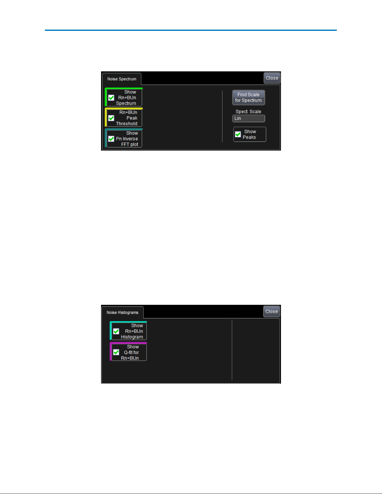
SDAIII-CompleteLinQ Software

Noise Spectrum

On the Noise Measurement dialog, touch the Noise Spectrum button to display the Noise Spectrum
dialog at the far right of the screen.

Show Rn+BUnSpectrum - Checking this box displays the Rn BUn Spectrum. This plot displays the
frequency spectrum of the signal with the data-dependent effects removed.

Rn+BUn Peak Threshold - Checking this box displays the threshold for the RnBUnSpectrum. Peaks higher
than this threshold are considered Pj and the remaining signal under the threshold is integrated to form
the Rj of the spectral method of jitter composition.

Show Pn Inv. FFT plot - Checking this box displays the Pn Inverse FFT. This plot is the inverse FFT of only
the points of the RnBUnSpectrum above the threshold. This allows you to view the peaks in the time
domain and is very useful for viewing time domain Pn effects.

Show Peaks - Checking this box displays the peaks of the RnBUnSpectrum. This annotates the points of
the RnBUnSpectrum above the threshold.

Noise Histogram Analysis

The RnBUn histogram can be viewed along with the Q-fit plot. RnBunHist is a histogram of the data in
the RnBUn track, and shows the distribution of the noise that is super-imposed on the data pattern.

Zoom the plot by touching the trace descriptor, and then selecting the zoom tab on the right side dialog.

Show Rn+BUn Histogram - Displays Rn+BUn Histogram. Vertical axis is in number of edges in a particular
jitter bin. Horizontal axis is the RnBUn jitter value. Scale is linear. Sometimes it is useful to use the log10
math function to get a log vertical scale to make it easier to view the tails.

Show Q-Fit for RnBUn- Plots the histogram in the Q-Scale representation. In the Q-Scale representation,
Gaussian tails result in straight lines whose slope is equal to 1/Rn. Teledyne LeCroy uses a special Q-scale
which we call nQ-Scale or normalized Q-Scale. This allows for Gaussian distributions with variable

52

921143 Rev A

Operator's Manual

populations or normalizations. Shown with the Q-scale transform is the best straight line fit (the thin
white line).

Noise Parameters

Touch the Noise Parameters button on the Noise Measurement dialog to display the Noise Parameters
mini-dialog.

NOTE: Noise measurements are computed using the dual-Dirac model chose in the Jitter Parameters
mini-dialog.

Show Rn - displays the random noise result. This is calculated either from the dual-Dirac analysis, or from
the RUnBUn spectrum, depending on the selection for the model to be used in the Jitter Parameters
dialog.

Show Dn - displays the deterministic noise result. This is calculated from dual-Dirac analysis analysis.

Show Tn(BER) - displays the total noise at the selected BER value. This corresponds to the noise one

would find when extrapolating the measured noise using one of three dual-Dirac models.

Show ISIn - displays the intersymbol interference "noise". This parameters quantifies the vertical extent
of ISI. (ISIis highly deterministic, but can look very much like noise, especially when looking at normal
data rather than a strictly repeating pattern.)

Show Pn - displays the periodic noise. This is the peak-to-peak height of the Pn inverse FFT.

Show EH(BER) - displays the eye height at the selected BER, calculated as the eye amplitude -Tn.

Show EW(BER) - displays the eye width at the selected BER, calculated as the unit interval width -Tj.

Log10 BER - This control sets the BER at which the Tnis reported, 10^-12 by default.

Turn Off All - Touch this button to turn off all noise parameters.

Noise Measurement Theory

Noise measurements and views are calculated using the algorithm described below.

1. Measuring noise requires an a priori knowledge of what component of the input waveform is signal
rather than noise. This is done via pattern analysis. In the simple case of a strictly repeating pattern,
such as PRBS7, which includes 127 bits, the oscilloscope can find the bit pattern in the waveform, and
identify all occurrences of any particular bit. When the data is not a repeating pattern, the oscil­loscope can look for repetitions of shorter runs to identify patterns By averaging the waveforms for
each bit in a pattern, (while taking into account small variations in the bit width due to PLL tracking),
a noiseless version of the pattern can be constructed.

921143 Rev A

53

SDAIII-CompleteLinQ Software

2. Subtracting the noiseless version of the pattern (iterated as necessary), from the original waveform
returns a noise waveform without data-dependent effects that cause relatively large variations in
amplitude from unit interval to unit interval. When retaining only the values of this waveform at a
selected position in each unit interval (the Sampling Phase), a waveform that contains the noise seen
by a receiver that samples or strobes each unit interval is created. This is the RnBUnTrack waveform,
which contains random and bounded uncorrelated noise, and which has data dependent effects
(which are highly deterministic) removed. The data can also be histogrammed to form the RnBUnHist
histogram. RUnBUnTrack and RnBUnHist can be used to understand sources of noise that can cause
bit errors, and can be enabled for display via the Noise Track and Noise Histogram dialogs. These
results are also the source data for the calculation of the noise measurements that are enabled in the
Noise Measurements dialog. The next steps in the measurement of these parameters follow closely
the algorithm that is used to measure and breakdown horizontal jitter.

3. The selection for the model used to calculate the jitter results is used in the noise measurements. In
the dual-Dirac spectral methods, the FFT of the RnBUnTrack is taken to create the RnBUnSpect spec­trum. Peaks in this spectrum above a calculated noise floor are associated with periodic noise, and
are removed and used to calculate a value for Pn. The remaining spectrum is used to form a raw
value of Rn by integrating (square root of the sum of the magnitudes squared). In the Rj Direct
method, this raw value (RnRaw) becomes the value of Rn itself. In the Rj+Dj CDF Fit method, the raw
value is used as a sigma value for fitting the tails of the RnBUn histogram.

4. The distribution of data dependent “noise” that was removed in the time domain by subtracting to
form the RnBUn trace is convolved with RnBUnHist to form an overall probability density function
(PDF). This is done independently for both the high and low levels, resulting in two PDFs .Integrating
these functions gives cumulative probability density functions, or CDFs for high and low levels. The
inner half of these distributions are taken and put together in order to form a CDF that provides infor­mation about the total noise that contributes to eye closure and bit errors.

5. In the Rj+Dj CDF Fit method, the CDF is then fit to the dual-Dirac equation Tn = alpha(BER) Rn + Dn,
using 4 values of BER about the user’s selected BER value to return values for Rn and Dn. In the Rj
Direct method, this fit is performed with the constraint that Rn = RnRaw.

6. When using the NQ-scale method, the tails of RnBUnHist are fitted to two Gaussian distributions that
can have both different sigmas and different populations. The data dependent noise is convolved in
as described above, and Tn, Rn and Dn is determined as described above for the Rj+Dj CDF Fit
method.

7. Pn is determined by taking the peaks found in step 3 above, and taking the iFFt. The peak-to-peak
amplitude resulting waveform is the periodic noise.

8. ISIn is determined by analyzing the distribution of voltages at the sampling phase, for the high and
low levels separately.

9. Tn is used to calculate an estimate of the eye opening at BER. The measurement Eye Height @ BER
(EH(BER)) is the Eye Amplitude-Tn.

10. Eye width @ BER (EW(BER)) is calculated by subtracting Tj from the unit interval width.

54

921143 Rev A

Operator's Manual

Crosstalk Measurements

Crosstalk Analysis

Crosstalk Analysis is part of the SDAIII-Crosstalk, SDAIII-CrossLinQ and and SDAII-CompleteLinQ prod­ucts. The dialog is accessed from the Crosstalk button on the main SDADialog.

The Crosstalk Eye shows the probabilistic extent of noise both inside and outside the eye, quickly show­ing the impact of excessive noise that is not possible to see in a traditional eye diagram. Inside the eye,
the analysis is identical as for the IsoBERthat can be added to the Eye diagram (see Eye Diagram Con-

figuration Dialog.)

Crosstalk Eye Algorithm

The crosstalk eye is formed using the following algorithm:

1. Perform pattern analysis to allow the identification of each bit in the pattern. This allows the deter­mination of all distinct trajectories the signal path can take. For example, a PRBS7 pattern has 127
bits, and 127 trajectories.

2. At 12 positions across the unit interval, calculate histograms of the signal amplitude for each bit in
the pattern.

3. Perform dual-Dirac analysis for each histogram to extrapolate the tails.

4. Integrate from the outside to the center of the the histograms to form CDFs.

5. Combine histograms for each of the 12 positions, forming 2 histograms at each position, one for the
0 state and one for the 1 state

6. For the selected BERvalues (as determined by the users selections for from, to and step), output the
voltage@BER on both sides of the CDF.

7. Connect the points corresponding to constant BER to form contour plots.

921143 Rev A

55

SDAIII-CompleteLinQ Software

Dialog Elements

from: Smallest BER value, which will correspond to the BER value of the contours furthest from the signal
trajectories

to: Largest BER value, which will correspond to the BERvalue of the contour closest to the signal tra­jectories.

step: Step size to use when move from the "From" value to the "To"value.

Show Crosstalk Eye - select to show the crosstalk eye for all enabled lanes.

Compare Crosstalk Eyes - Touch to open a window that overlays two crosstalk eyes for comparison.

56

921143 Rev A