Tektronix TDSJIT3 v2 User manual

Download

Online Help

TDSJIT3 v2 Jitter Analysis Application

PHP025510

Adapted from the TDSJIT3 v2 Help,Version 1.0.1 (November, 2004)

www.tektronix.com

Copyright © Tektronix, Inc. All rights reserved. Licensed software products are owned by Tektronix or its suppliers and are protected by United States copyright laws and international treaty provisions.

Use, duplication, or disclosure by the Government is subject to restrictions as set forth in subparagraph (c)(1)(ii) of the Rights in Technical Data and Computer Software clause at DFARS 252.227-7013, or subparagraphs (c)(1) and (2) of the Commercial Computer Software -- Restricted Rights clause at FAR 52.227-19, as applicable.

Tektronix products are covered by U.S. and foreign patents, issued and pending. Information in this documentation supercedes that in all previously published material. Specifications and price change privileges reserved.

Tektronix, Inc. P.O. Box 500, Beaverton, OR 97077

TEKTRONIX, TEK, and RT-Eye are registered trademarks of Tektronix, Inc.

TDSJIT3 v2 Jitter Analysis Online Help, OLH0255, Version 1.0.1

General Safety Summary...................................................................... xi

Preface ..................................................................................................xiii

5-Time Free Trial.............................................................................................. xiii

Related Documentation..................................................................................... xiii

GPIB Information ..............................................................................................xiv

Relevant Web Sites............................................................................................xiv

Application CD Contents...................................................................................xiv

Conventions ........................................................................................................xv

Types of Online Help Information......................................................................xv

Using Online Help .............................................................................................xvi

Find Tab and Searches..................................................................................... xvii

Contacting Tektronix ....................................................................................... xvii

Feedback......................................................................................................... xviii

Getting Started

Operating Basics

Differences between TDSJIT3 v2 Advanced and TDSJIT3 v2 Essentials ...........1

Compatibility ........................................................................................................2

Requirements and Restrictions .............................................................................2

Accessories ...........................................................................................................2

Installation ............................................................................................................2

Connecting to a Device Under Test (DUT) ...................................................3

Deskewing Probes and Channels...................................................................3

General Information..............................................................................................5

Starting the TDSJIT3 v2 Application ............................................................5

Returning to the Application .........................................................................6

Minimizing and Maximizing the Application................................................6

Exiting the Application..................................................................................6

Application Directories and Usage ................................................................6

Tips on the TDSJIT3 v2 User Interface.........................................................8

How to Enter Numeric Values.......................................................................9

Virtual Keypad ..............................................................................................9

Using Basic Oscilloscope Functions............................................................10

File Menus ...................................................................................................10

Navigating the User Interface .............................................................................10

General Steps to Set Up the Application .....................................................11

Jitter Wizard ................................................................................................11

User Interface Information ..........................................................................13

Setting Up the Application for Analysis .............................................................15

Selecting Measurements ..............................................................................15

Configuring a Measurement ........................................................................19

Configuring Sources ....................................................................................36

Measurement Summaries.............................................................................48

TDSJIT3 v2 Jitter Analysis Online Help i

Table of Contents

Taking Measurements.........................................................................................48

Localizing Measurements ............................................................................49

About Sequencing........................................................................................49

Acquiring Data ............................................................................................49

New Acquisition Function of the Single Button ..........................................50

Control Panel Functions ..............................................................................50

Clearing Results...........................................................................................51

Results as Statistics .............................................................................................52

Viewing Equivalent Rj/Dj Results (TDSJIT3 v2 Advanced Only) .............52

Results as Plots ...................................................................................................53

Using a Separate Monitor to View Plots .....................................................54

Plot Usage....................................................................................................54

Creating Plots ..............................................................................................56

Configuring Plots.........................................................................................57

Working with Plots .............................................................................................62

Toolbar Functions in Plot Windows ............................................................63

Selecting and Viewing a Plot.......................................................................63

Moving and Resizing a Plot.........................................................................64

Deleting Plots ..............................................................................................64

Using Zoom in a Plot...................................................................................65

Using Cursors in a Plot ................................................................................66

Exporting Plot Files .....................................................................................69

Saving Information to Log Files.........................................................................71

Logging Statistics ........................................................................................71

Logging Measurements ...............................................................................72

Logging Worst Case Waveforms.................................................................73

File Names for Logging Worst Case Waveforms........................................74

Saving and Recalling Setup Files .......................................................................74

Saving a Setup File ......................................................................................74

Recalling a Saved Setup File .......................................................................75

Recalling the Default Setup .........................................................................76

Recalling a Recently Saved or Accessed Setup File....................................76

Recall Recent Files Example .......................................................................77

Recalling a Setup File from a Prior Version of Software ............................77

Docking and Undocking the Jitter Analysis Window..................................78

Acquisition Timeout Utility.........................................................................78

Warnings Utility ..........................................................................................78

Tutorial

Setting Up the Oscilloscope................................................................................79

Starting the Application ...............................................................................79

Waveform Files ...........................................................................................79

Recalling a Waveform File ..........................................................................79

Taking a Clock Period Measurement..................................................................81

Setting Up a Period Measurement ...............................................................81

Taking a Period Measurement and Viewing Statistical Results ..................83

Viewing a Period Measurement as Plots .....................................................84

Ending a Tutorial Lesson ....................................................................................86

TDSJIT3 v2 Jitter Analysis Online Help

Table of Contents

Taking a Clock-to-Output Time Measurement ...................................................86

Setting Up and Taking a Clock-to-Output Time Measurement ...................86

Logging Statistics to a .CSV File ................................................................89

Logging Data Points as a Measurement Snapshot to a .CSV File ...............92

Logging Worst Case Waveforms to .WFM Files ........................................94

Lessons Learned .................................................................................................97

Application Examples

Recall Default Settings .......................................................................................99

Recall a Waveform and Start the Application ....................................................99

Application Example 1: Spectral Analysis .......................................................100

Set Up and Take Measurements for Example 1.........................................100

Approximate Pattern Length Measured with Cursors................................101

Measuring Rj/Dj and Tj @ BER................................................................102

Using Spectral Analysis to Find Jitter Sources..........................................103

Application Example 2: Trend Analysis...........................................................105

Set Up and Take Measurements for Example 2.........................................105

Using Trend Analysis to Find Jitter Amplitude and Anomalies................106

Algorithms

Oscilloscope Setup Guidelines .........................................................................109

Test Methodology.............................................................................................109

Timing Measurements ......................................................................................110

Rj/Dj Measurement (TDSJIT3 v2 Advanced Only) ..................................110

Spectrum Analysis Based Rj/Dj Separation ..............................................110

Arbitrary Pattern Analysis Based Rj/Dj Separation...................................111

BER and Tj Estimation (TDSJIT3 v2 Advanced Only) ............................112

Effective Rj and Tj Estimation (TDSJIT3 v2 Advanced only)..................113

Single Waveform Measurements......................................................................113

Clock Period Measurement........................................................................113

Clock Frequency Measurement .................................................................114

Clock TIE Measurement............................................................................114

Clock PLL TIE Measurement (TDSJIT3 v2 Advanced Only) ..................114

Data Period Measurement..........................................................................115

Data Frequency Measurement ...................................................................115

Data TIE Measurement..............................................................................115

Data PLL TIE Measurement (TDSJIT3 v2 Advanced Only) ....................115

Cycle-to-Cycle Measurement ....................................................................116

N-Cycle Measurement...............................................................................116

Positive and Negative Cycle-to-Cycle Duty Measurements......................116

Positive and Negative Duty Cycle Measurements .....................................117

Rise Time Measurement ............................................................................117

Fall Time Measurement .............................................................................117

Positive and Negative Width Measurements .............................................118

High Time Measurement ...........................................................................118

Low Time Measurement............................................................................118

TDSJIT3 v2 Jitter Analysis Online Help

iii

Table of Contents

Parameters

Dual Waveform Measurements ........................................................................119

Setup Time Measurement ..........................................................................119

Hold Time Measurement ...........................................................................119

Clock-to-Output Measurement ..................................................................120

Skew Measurement....................................................................................120

Crossover Voltage Measurement (TDSJIT3 v2 Advanced Only) .............120

Statistics............................................................................................................121

Maximum Value ........................................................................................121

Minimum Value.........................................................................................121

Mean Value ...............................................................................................121

Standard Deviation Value..........................................................................121

Maximum Positive and Maximum Negative Difference Values ...............122

Peak-to-Peak Value ...................................................................................122

Population Value .......................................................................................122

File Menus Parameters......................................................................................123

Control Panel Parameters..................................................................................124

Measurements Select ........................................................................................124

Configure Measurements..................................................................................125

Clock Recovery Parameters.......................................................................126

Advanced Clock Recovery Parameters......................................................127

Filters Parameters ......................................................................................127

Advanced Filter Parameters.......................................................................127

TIE: RjDj Analysis Parameters (TDSJIT3 v2 Advanced Only) ................128

Configure Sources ............................................................................................128

Summaries ........................................................................................................130

Results ..............................................................................................................130

Plots ..................................................................................................................130

Logs ..................................................................................................................132

Utilities .............................................................................................................133

Help ..................................................................................................................134

GPIB

Index

Program Example .............................................................................................135

GPIB Reference Materials ................................................................................136

Starting and Setting Up the Application Using GPIB................................136

Variable:Value Command ................................................................................136

Measurements Results Queries .........................................................................142

TDSJIT3 v2 Jitter Analysis Online Help

Table of Contents

List of Figures

Figure 1: Contents of the application CD-ROM............................................ xiv

Figure 2: Deskew complete example.................................................................. 4

Figure 3: Deskew Summary example................................................................4

Figure 4: Starting the TDSJIT3 v2 application ................................................ 5

Figure 5: Returning to the application ..............................................................6

Figure 6: Directory structure ............................................................................7

Figure 7: On-screen keypad................................................................................ 9

Figure 8: General steps to set up the application........................................... 11

Figure 9: Jitter Wizard when launched........................................................... 12

Figure 10: Menu with user interface items...................................................... 14

Figure 11: Menu navigation tree...................................................................... 14

Figure 12: Measurements Select menu........................................................... 16

Figure 13: Select Source options by measurement category.......................... 16

Figure 14: Clock edge options ..........................................................................21

Figure 15: Active edge options.......................................................................... 21

Figure 16: Clock and Data edge options.......................................................... 22

Figure 17: From Edge and To Edge options ................................................... 22

Figure 18: Main edge options ........................................................................... 23

Figure 19: Meas Range Limits options ............................................................ 23

Figure 20: N-Cycle measurement options .......................................................24

Figure 21: Bathtub Curve and BER versus Decision Time ........................... 26

Figure 22: TIE: RjDj analysis options for Clock TIE and

Clock PLL TIE ...........................................................................................27

Figure 23: TIE: RjDj analysis options for Data TIE and Data PLL TIE.....27

Figure 24: Constant Clock Recovery concept .................................................28

Figure 25: Reference Clock Frequency options.............................................. 29

Figure 26: Phase-Locked Loop (PLL) Clock Recovery concept ................... 29

Figure 27: PLL Loop Bandwidth options........................................................ 30

Figure 28: Advanced Clock Recovery options ................................................ 32

Figure 29: Optional filters................................................................................. 32

Figure 30: Filter characteristics ....................................................................... 33

Figure 31: Band Pass filtering ..........................................................................33

Figure 32: Filters options.................................................................................. 34

Figure 33: Advanced Filter options..................................................................35

Figure 34: Effect of the Smoothing window .................................................... 36

Figure 35: Configure Sources Autoset options................................................39

Figure 36: Configure Sources Gating options................................................. 40

TDSJIT3 v2 Jitter Analysis Online Help

Table of Contents

Figure 37: Reference voltage levels diagram...................................................41

Figure 38: Example of Hysteresis on a noisy waveform................................. 42

Figure 39: Autoset Ref Levels options ............................................................. 45

Figure 40: Configure Sources Ref Levels options........................................... 47

Figure 41: Configure Sources Stat pop Limit options.................................... 48

Figure 42: Control Panel options ..................................................................... 51

Figure 43: Plots Create menu........................................................................... 57

Figure 44: Vert/Horiz menu for a Histogram plot.......................................... 58

Figure 45: Vert/Horiz menu for a Time Trend plot ....................................... 59

Figure 46: Vert/Horiz menu for a Spectrum plot........................................... 59

Figure 47: Vert/Horiz menu for a Bathtub plot.............................................. 60

Figure 48: Transfer Function Definition options............................................ 61

Figure 49: Vert/Horiz menu for a Transfer Function plot ............................61

Figure 50: Vert/Horiz menu for a Phase Noise plot........................................ 62

Figure 51: Locate Window At options............................................................. 63

Figure 52: File Save browser ............................................................................ 75

Figure 53: File Recall browser.......................................................................... 76

Figure 54: Recall Recent files example ............................................................ 77

Figure 55: Acquisition Timeout options .......................................................... 78

Figure 56: Oscilloscope Reference Memory options ......................................80

Figure 57: Clock Period measurement selected .............................................. 82

Figure 58: Configuration of a Period measurement....................................... 82

Figure 59: Configure Sources Ref Levels before an autoset.......................... 82

Figure 60: Configure Sources Ref Levels after an autoset............................. 83

Figure 61: Statistical results for a Clock Period measurement..................... 83

Figure 62: Min/Max statistical results for a Clock Period measurement..... 84

Figure 63: Mean/Std. Dev statistical results for a Clock Period

measurement............................................................................................... 84

Figure 64: Create plots of results ..................................................................... 85

Figure 65: Results as a Histogram plot............................................................ 85

Figure 66: Results as a Time Trend plot..........................................................85

Figure 67: Results as a Spectrum plot .............................................................86

Figure 68: Clock-to-Output measurement selected........................................ 87

Figure 69: Configuration of a Clock-to-Output measurement...................... 88

Figure 70: Statistical results for a Clock-to-Output measurement............... 88

Figure 71: Configure Sources Ref Levels for a Clock-to-Output

measurement............................................................................................... 88

Figure 72: Measurements Summary for a Clock-to-Output

measurement............................................................................................... 89

Figure 73: Ref Levels Summary for a Clock-to-Output measurement.........89

TDSJIT3 v2 Jitter Analysis Online Help

Table of Contents

Figure 74: Log Statistics for a Clock-to-Output measurement ..................... 90

Figure 75: Log File Name dialog ...................................................................... 90

Figure 76: Path to the stats.csv log file............................................................. 91

Figure 77: Viewing statistics in a spreadsheet program.................................91

Figure 78: Log Measurement /configure menu for a Clock-to-Output

measurement............................................................................................... 92

Figure 79: Input Directory Name dialog ......................................................... 93

Figure 80: Save Current Measurements dialog .............................................. 93

Figure 81: Path to the TC01R1R2.csv log file................................................. 94

Figure 82: Viewing a data log file in a spreadsheet program ........................ 94

Figure 83: Log Worst Case Waveforms configuration for a

Clock-to-Output measurement ................................................................. 95

Figure 84: Log Worst Case Waveforms dialog............................................... 96

Figure 85: Path to the worse case .wfm log files .............................................96

Figure 86: Data Period results for example 1................................................101

Figure 87: Pattern Length for example 1 ...................................................... 102

Figure 88: Rj/Dj results for example 1...........................................................103

Figure 89: Spurs for example 1 ......................................................................104

Figure 90: Data Period results for example 2................................................106

Figure 91: Time Trend plot for example 2 .................................................... 107

TDSJIT3 v2 Jitter Analysis Online Help

vii

Table of Contents

List of Tables

Table 1: Directories and usage .........................................................................7

Table 2: File name extensions............................................................................8

Table 3: Entering numeric values .....................................................................9

Table 4: File menus...........................................................................................10

Table 5: User interface items...........................................................................13

Table 6: Measurement definitions ..................................................................17

Table 7: General measurement definitions ...................................................18

Table 8: File menus...........................................................................................19

Table 9: Configure Measurement menus and applicable

measurements....................................................................................................20

Table 10: N-Cycle measurement configuration .............................................24

Table 11: TIE: RjDj analysis configuration...................................................26

Table 12: Reference Clock Frequency configuration ....................................28

Table 13: PLL Loop Bandwidth configuration..............................................30

Table 14: Advanced Clock Recovery configuration ......................................31

Table 15: Filters configuration........................................................................34

Table 16: Advanced Filter configuration........................................................35

Table 17: Configure Sources menus ...............................................................37

Table 18: Configure Sources Autoset configuration .....................................38

Table 19: Optimize Horizontal For configuration.........................................39

Table 20: Configure Sources Gating configuration.......................................40

viii

Table 21: Configure Sources Qualify configuration......................................40

Table 22: Configure Sources Ref Levels Autoset configuration...................43

Table 23: Configure Sources Ref Levels Autoset configuration...................44

Table 24: Configure Sources Ref Levels configuration.................................46

Table 25: Configure Sources Stat pop Limit configuration..........................47

Table 26: Measurement Summaries menus ...................................................48

Table 27: Control Panel functions...................................................................50

Table 28: Statistics menus................................................................................52

Table 29: Plot types ..........................................................................................53

Table 30: Measurements and available plots .................................................54

Table 31: Plots Create menu options ..............................................................57

Table 32: Vert/Horiz axis options for a Histogram plot................................58

Table 33: Vert/Horiz axis options for a Time Trend plot .............................58

Table 34: Vert/Horiz axis options for a Spectrum plot.................................59

Table 35: Vert/Horiz axis options for a Bathtub plot....................................60

Table 36: Transfer Function Definition configuration..................................60

Table 37: Vert/Horiz axis options for a Transfer Function plot ..................61

TDSJIT3 v2 Jitter Analysis Online Help

Table of Contents

Table 38: Vert/Horiz axis options for a Phase Noise plot..............................62

Table 39: Log Statistics configuration ............................................................72

Table 40: Log Measurements configuration ..................................................73

Table 41: Log Worst Case Waveforms configuration ...................................74

Table 42: Single waveform measurements...................................................113

Table 43: Dual waveform measurements .....................................................119

Table 44: File menus parameters..................................................................123

Table 45: Select Source area parameters .....................................................124

Table 46: Math Defs area parameters ..........................................................125

Table 47: Waveform Edges parameters .......................................................125

Table 48: Measurement Range Limits parameters .....................................125

Table 49: N-Cycle measurement parameters...............................................126

Table 50: Clock Recovery: Reference Clock Frequency parameters ........126

Table 51: Clock Recovery: Loop BW parameters......................................126

Table 52: Advanced Clock Recovery parameters........................................127

Table 53: Filters parameters..........................................................................127

Table 54: Advanced Filter parameter...........................................................127

Table 55: TIE: RjDj Analysis parameters (TDSJIT3 v2 Advanced only).128

Table 56: Configure Sources Autoset parameters.......................................128

Table 57: Configure Sources Gate/Qualify parameters ..............................129

Table 58: Configure Sources Ref Levels parameters ..................................129

Table 59: Configure Stat Pop Limit parameters .........................................129

Table 60; Configure Ref Level Autoset Setup Menu parameters ..............130

Table 61 Histogram Vert/Horiz Axis menu parameters .............................131

Table 62: Time Trend Vert/Horiz Axis menu parameter...........................131

Table 63: Spectrum Vert/Horiz Axis menu parameters .............................131

Table 64: Bathtub Vert/Horiz Axis menu parameters................................131

Table 65: Transfer Function Vert/Horiz Axis menu parameters...............132

Table 66: Phase Noise Vert/Horiz Axis menu parameters..........................132

Table 67: Log Statistics menu parameters ...................................................132

Table 68: Log Measurements Configure menu parameters .......................133

Table 69: Log Worst Case Waveforms Configure menu parameters........133

Table 70: Deskew menu parameters .............................................................134

Table 71: Acq Timeout menu parameters....................................................134

Table 72: Variable:Value JITTER3 command arguments and queries

part 1 ...............................................................................................................135

Table 73: Variable:Value JITTER3 command arguments and queries

part 2................................................................................................................136

Table 74: Variable:Value JITTER3 command arguments and queries

part 3................................................................................................................137

TDSJIT3 v2 Jitter Analysis Online Help

Table of Contents

Table 75: Variable:Value JITTER3 command arguments and queries

part 4................................................................................................................138

Table 76: Variable:Value JITTER3 command arguments and queries

part 5................................................................................................................141

Table 77: Measurement result queries..........................................................144

Table 78: Measurement names and keys......................................................144

Table 79: Source names and key..................................................................144

Table 80: Plot names and key ........................................................................144

Table 81: Error codes....................................................................................145

TDSJIT3 v2 Jitter Analysis Online Help

General Safety Summary

Review the following safety precautions to avoid injury and prevent damage to this product or any products connected to it. To avoid potential hazards, use this product only as specified.

Only qualified personnel should perform service procedures.

While using this product, you may need to access other parts of the system. Read the General Safety Summary in other system manuals for warnings and cautions related to operating the system.

To Avoid Fire or Personal Injury:

Connect and Disconnect Properly: Do not connect or disconnect probes or test leads while they are connected to a voltage source.

Observe All Terminal Ratings: To avoid fire or shock hazard, observe all ratings and markings on the product. Consult the product manual for further ratings information before making connections to the product.

Do Not Operate With Suspected Failures: If you suspect there is damage to this product, have it inspected by qualified service personnel.

Symbols and Terms: The following terms and symbols may appear in the online help.

WARNING: Warning statements identify conditions or practices that could

result in injury or loss of life.

CAUTION: Caution statements identify conditions or practices that could

result in damage to this product or other property.

Terms on the Product: The following terms may appear on the product:

DANGER indicates an injury hazard immediately accessible as you read the marking.

WARNING indicates an injury hazard not immediately accessible as you read the marking.

CAUTION indicates a hazard to property including the product.

Symbols on the Product: The following symbol may appear in the product:

CAUTION Refer to Help

TDSJIT3 v2 Jitter Analysis Online Help xi

General Safety Summary

xii

TDSJIT3 v2 Jitter Analysis Online Help

Preface

5-Time Free Trial

The TDSJIT3 v2 application consists of two products: Jitter Analysis Advanced and Jitter Analysis Essentials. These products are applications that enhance basic capabilities of some Windows-based oscilloscopes from Tektronix. These jitter analysis applications include the following features:

• Select and configure multiple measurements on more than one waveform

• Display statistical results for up to six measurements

• Perform random and deterministic jitter analysis including BER estimation

(TDSJIT3 v2 Advanced only)

• Show results as plots

• Save statistical results to a data log file

• Save individual data points to a measurement results file

• Save the worst case waveforms to .wfm files

A 5-time free trial is available for all applications in the "Applications on this CD and Compatible Oscilloscope" table found in the Optional Applications Software on a Windows Based Oscilloscope Installation Manual (accessible as a PDF file.) You can start and exit an application up to five times to help you evaluate Tektronix software solutions.

If an application becomes available after you receive your oscilloscope, you can download the application as described in the installation manual to try the free trial.

GPIB Information

Relevant Web Sites

For information on how to operate the oscilloscope and use the applicationspecific GPIB commands, refer to the following items:

• The user manual for your oscilloscope provides general information on how to

operate the oscilloscope.

• The online help for your oscilloscope can provide details on how to use GPIB

commands to control the oscilloscope if you install the GPIB Programmer guide (and code examples) from the oscilloscope CD-ROM.

• The example directory for programming examples of how to remotely control

the application. The default location for the example files is C:\TekApplications\TDSJIT3v2\Examples\GPIB-Examples.

The Tektronix web site offers the following information:

• Understanding and Characterizing Jitter Primer, part number 55W-16146-0

• Jitter analysis details on the www.tektronix.com/jitter web page

You can also find useful information in the Fibre Channel - Methodologies for Jitter and Signal Quality Specification – MJSQ on the www.t11.org web site.

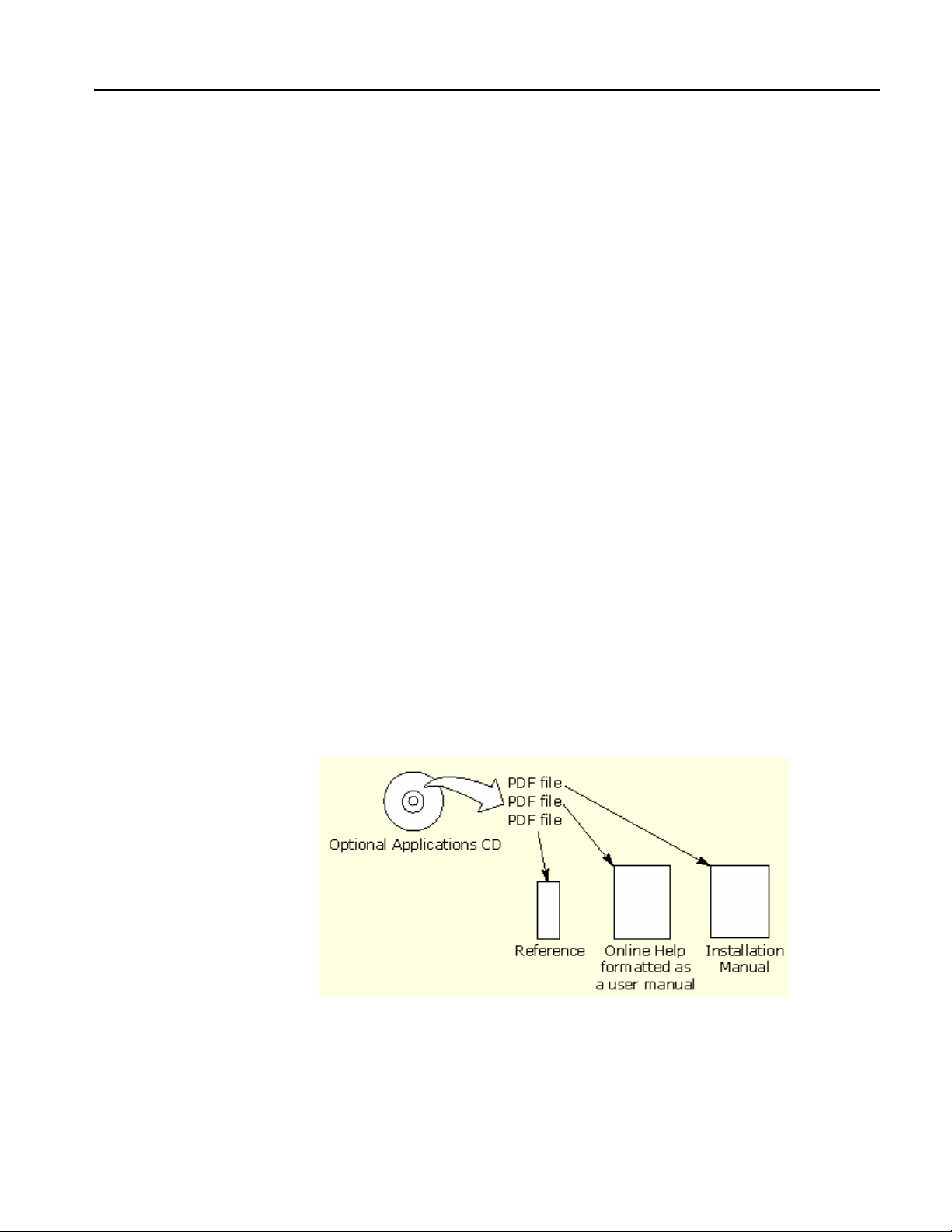
Application CD Contents

The Optional Applications Software on a Windows Based Oscilloscope CD-ROM includes files for the following types of documentation:

• Printable file of the TDSJIT3 v2 Jitter Analysis online help formatted to

• Reference guides

• Optional Applications Installation manual

resemble a user manual

xiv

Figure 1: Contents of the application CD-ROM

TDSJIT3 v2 Jitter Analysis Online Help

Preface

You can use the following methods to view most PDF files associated with this application:

• Access a file in the Documents directory on the Optional Applications

Software on a Windows-Based Oscilloscope CD-ROM from any PC

• Access a file from the CD Installation Browser

• Select a file (except Reference guides) from the Start menu in the oscilloscope

task bar; you may need to minimize the oscilloscope and minimize the application

• Use the Manuals Finder from the www.tektronix.com web site.

You can also use this additional method to view only the PDF file of the online help:

• Select the shortcut on the desktop of the oscilloscope after you minimize the

oscilloscope

Note: If you do not have an Acrobat reader to view a PDF file, you can get a free copy of the reader from the www.adobe.com/products/acrobat web page.

Conventions

Online help topics use the following conventions:

• The terms "TDSJIT3 v2 application" or "application" refer to the TDSJIT3 v2

Advanced or TDSJIT3 v2 Essentials Jitter Analysis Application (except when noted as Advanced only)

• The term "oscilloscope" refers to any product on which this application runs.

• The term "select" is a generic term that applies to the two mechanical methods

of choosing an option: with a mouse or with the Touch Screen.

• The term "DUT" is an abbreviation for Device Under Test.

• User interface screen graphics are from a TDS7000 series oscilloscope; there

may be minor differences in the displays on other types of oscilloscopes.

• When steps require a sequence of selections using the application interface,

the ">" delimiter marks each transition between a menu and an option. For example, one of the steps to recall a setup file would appear as File> Recall.

Types of Online Help Information

The online help contains the following types of information:

• A Getting Started group of topics briefly describes the application, contains

connection procedures, and includes a deskew procedure.

• An Operating Basics group of topics covers basic operating principles of the

application, including the Jitter Wizard. The sequence of topics reflects the steps you perform to operate the application and includes definitions for all menus and options.

• A Tutorial group of topics teaches you how to set up the application to acquire

a waveform, take a measurement, view the results, view a plot, and save data to a file.

TDSJIT3 v2 Jitter Analysis Online Help

Preface

Using Online Help

• An Application Examples group of topics demonstrates how to use jitter

measurements to identify a problem with a waveform. This should give you ideas on how to solve your own measurement problems.

• A Reference group of topics specifies the minimum, maximum, incremental,

or list of choices, and the default values for all adjustable parameters.

• A Measurement Algorithms group of topics includes measurement guidelines

and information on how the application calculates each measurement.

• A GPIB Command Syntax group of topics contains a list of arguments and

values that you can use with the remote commands and their associated parameters. The application includes simple remote interface programs to show you how to operate the application using GPIB commands.

The application installs a desktop shortcut to access a PDF file of the help topics. The file is printable and is formatted to resemble a user manual.

Online help has many advantages over a printed manual because of advanced search capabilities. You can select Help> Topics on the right side of the application menu bar to display the Help file.

The main (opening) Help screen shows a series of book icons and three tabs along the top menu, each of which offers a unique mode of assistance:

• Table of Contents (TOC) tab - organizes the Help into book-like sections.

Select a book icon to open a section; select any of the topics listed under the book.

• Index tab - enables you to scroll a list of alphabetical keywords. Select the

topic of interest to display the corresponding help page.

• Find tab - allows a text-based search. Follow these steps:

1. Type the word or phrase you wish to find in the search box.

If the word or phrase is not found, try the Index tab.

2. Select some matching words in the next box to narrow your search.

3. Choose a topic in the lower box, and then select the Display button.

Note: The Find tab function does not include words found in graphics. Refer to the Find Tab and Searches topic for more information.

A Note: in the topic text indicates important information.

When you use a mouse, you can tell when the cursor is over an active

hyperlink because the arrow cursor changes to a small pointing hand cursor.

The light bulb icon and word Tip in the graphic above indicates additional information to help you operate the application more efficiently.

xvi

TDSJIT3 v2 Jitter Analysis Online Help

Preface

Find Tab and Searches

Many online help topics only contain tables. To retain vertical and horizontal lines, the tables are graphical objects. The Find tab in the online help does not recognize words in these tables.

The online help is extensively indexed with the proper names of all menus and options as they appear in the application and in the left column of graphical tables.

Note: If you conduct a Find tab search with no results, try the Index tab instead.

Contacting Tektronix

Phone Address

Web site Sales support Service support Technical support

* This Telephone number is toll free in North America. After office hours, please leave a voice mail message.

Outside North America, contact a Tektronix sales office or distributor; See the Tektronix web site for a list of offices.

1-800-833-9200*

Tektronix, Inc. Department or name (if known) 14200 SW Karl Braun Drive P.O. Box 500 Beaverton, OR 97077 USA

www.Tektronix.com

1-800-833-9200, select option 1*

1-800-833–9200, select option 2*

www.tektronix.com/support 1-800-833-9200, select option 3*

6:00 a.m. - 5:00 p.m. Pacific time

TDSJIT3 v2 Jitter Analysis Online Help

xvii

Preface

Feedback

Tektronix values your feedback on our products. To help us serve you better, please send us suggestions, ideas, or other comments you may have about your application or oscilloscope.

You can email your feedback to techsupport@tektronix.com, FAX at (503) 6275695, or by phone. Please be as specific as possible and include the following information:

General Information

• Oscilloscope model number and hardware options, if any

• Probes used

• Serial data standard

• Signaling rate

• Your name, company, mailing address, phone number, FAX number

Note: Please indicate if you would like to be contacted by Tektronix regarding your suggestion or comments.

Application-Specific Information

• Software version number

• Description of the problem such that technical support can duplicate the

problem

• If possible, save the oscilloscope waveform file as a .wfm file

• If possible, save the oscilloscope and application setup files from the

application to obtain both the oscilloscope .set file and the application .ini file. Refer to Saving a Setup File.

Once you have gathered this information, you can contact technical support by phone or through e-mail. If using e-mail, be sure to enter "TDSJIT3 v2 Problem" in the subject line, and attach the .set, .ini, and .wfm files.

To include screen shots, from the oscilloscope menu bar, select File> Export. In the Export dialog box, enter a file name with a .bmp extension and select Save. The file is saved in the C:\TekScope\Images directory. You can then attach the file to your email (depending on the capabilities of your email editor).

xviii

TDSJIT3 v2 Jitter Analysis Online Help

Getting Started

The TDSJIT3 v2 application consists of two products: Jitter Analysis Advanced and Jitter Analysis Essentials. These products are applications that enhance basic capabilities of some Windows-based oscilloscopes from Tektronix. The application includes a Wizard to help you quickly set up measurements and obtain measurement results.

You can use this application to do the following tasks:

• Select and configure multiple measurements on one or more waveforms

• Display statistical results for up to six measurements

• Perform random and deterministic jitter analysis including BER estimation

(TDSJIT3 v2 Advanced only)

• Apply high pass and low pass filters to the measurements (TDSJIT3 v2

Advanced only)

• Display the results as Histogram, Time Trend, Cycle Trend, and Spectrum

plots; for TDSJIT3 v2 Advanced only, also display the results as Bathtub, Transfer Function, and Phase Noise plots

• Export plots

• Log statistical results to a file

• Log individual data points to a measurement results file

• Log worst case waveforms to files

Note: There are no standard accessories for this product.

Differences between TDSJIT3 v2 Advanced and TDSJIT3 v2 Essentials

The TDSJIT3 v2 Advanced application provides the following features that are not included in the TDSJIT3 v2 Essentials application:

• PLL-Based Clock Recovery

• Crossover Voltage Analysis

• Jitter separation (Rj/Dj analysis)

• Bit error rate estimation (BER)

• Filters

• Bathtub, Transfer Function, and Phase Noise plots

Features that are only available with the TDSJIT3 v2 Advanced application are indicated as "TDSJIT3 v2 Advanced only."

TDSJIT3 v2 Jitter Analysis Online Help 1

Getting Started

Compatibility

For information on oscilloscope compatibility, refer to the product data sheet (use the Search tool on the www.tektronix.com web site).

The setup files for TDSJIT3 v2 Advanced and TDSJIT3 v2 Essentials are compatible with each other.

The TDSJIT3 v2 Advanced application will recall setup files made with previous versions of TDSJIT3 and TDSJIT3E. To convert an existing setup file, recall it and then save it again. If you wish to retain a copy of the original setup file, use a different filename when saving. Note that setup files from previous versions may include directory paths such as "C:\TekApplications\TDSJIT3\...", whereas the v2 application defaults to "C:\TekApplications\TDSJIT3v2\...". If you would like your converted setup files to use the TDSJITv2 directory, recall the existing setup file, use the Graphical User Interface to change any file paths to use the new directory structure, and then save the setup.

Requirements and Restrictions

The Sun Java Run-Time Environment (JRE) V1.4.2 must be installed on the oscilloscope to operate the TDSJIT3 v2 application. When you install the application, the InstallShield Wizard automatically installs the proper version of the JRE. If the JRE is deleted, install TDSJIT3 v2 application again.

Accessories

Installation

Memory. A minimum of 512 MB PC memory is required and 1 GB PC memory is highly recommended.

Keyboard. You will need to use a keyboard to enter new names for some file save operations.

There are no standard accessories for this product. However, you can refer to the product datasheet available on the Tektronix web site for information on optional accessories relevant to your application.

Refer to the Optional Applications Software on a Windows-Based Oscilloscope Installation Manual for the following information:

• List of available applications, compatible oscilloscopes, and version numbers

• How to use the 5-time free trials

• How to apply a new authorized Option Installation key label

• Installation procedures

• How to enable an application

• How to download updates from the Tektronix web site

TDSJIT3 v2 Jitter Analysis Online Help

Getting Started

Connecting to a Device Under Test (DUT)

You can use any compatible probes or cable interface to connect between your DUT and oscilloscope. One connection is sufficient for most signals.

The Clock-to-Output, Skew, and Crossover Voltage (TDSJIT3 v2 Advanced only) measurements require two input channels, two reference, or two Math waveforms.

Warning: To avoid electric shock, remove power from the DUT before attaching probes. Do not touch exposed conductors except with the properly rated probe tips. Refer to the probe manual for proper use.

Refer to the General Safety Summary in your oscilloscope manual.

Deskewing Probes and Channels

To ensure accurate results for two-channel measurements, it is important to first deskew the probes and oscilloscope channels before you take measurements from your DUT.

The application includes an automated deskew utility that you can use to deskew any pair of oscilloscope channels.

Note: To produce the best deskew results, you should connect the probes to the fastest signal in your DUT.

Deskewing on Oscilloscopes with Bandwidth Extension

Some Tektronix oscilloscopes feature software-based bandwidth extension. The bandwidth extension may be enabled on a per-channel basis.

Enabling or disabling bandwidth extension on any channel affects the skew on that channel. Thus, you should deskew probes and channels after you make such configuration changes.

Steps to Deskew Probes and Channels

To deskew a pair of probes and oscilloscope channels, follow these steps:

1. Refer to Connecting to a Device Under Test before starting the procedure.

2. Connect both probes to the fastest signal in your DUT.

Set up the oscilloscope as follows:

1. Use the Horizontal Scale knob to set the oscilloscope to an acquisition rate so

that there are two or more samples on the deskew edge.

2. Use the Vertical Scale and Position knobs to adjust the signals to fill the

display without missing any part of the signals.

3. Set the Record Length so that there are more than 100 edges in the

acquisition.

4. Start the TDSJIT3 v2 application.

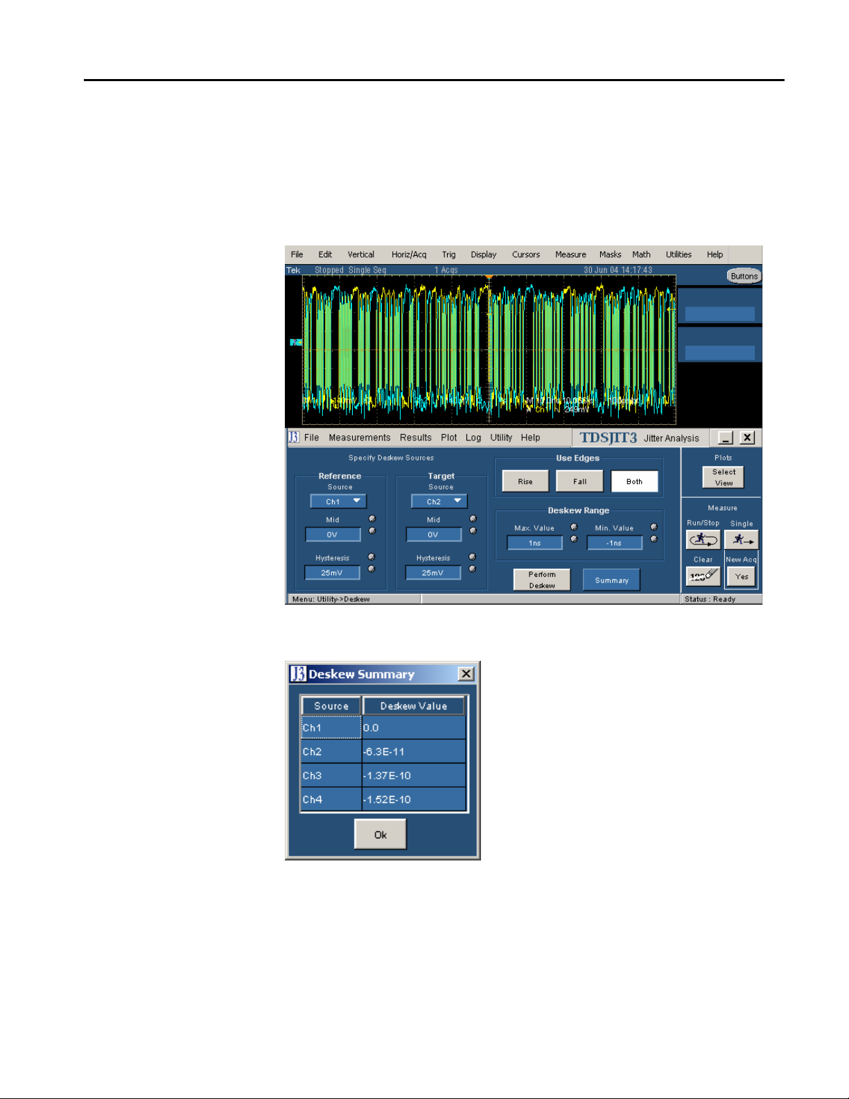
5. Select Utilities> Deskew. The Deskew Utility menu appears.

6. Set the Reference Source option to Ch1. The Source waveform is the

reference point used to deskew the remaining channels.

TDSJIT3 v2 Jitter Analysis Online Help

Getting Started

7. Set the Target Source option to Ch2. This is the channel that will be

deskewed.

8. To start the utility, select the Perform Deskew command button, and then

select Yes.

9. Repeat steps 7 and 8 for Ch3, and then for Ch4 to deskew those channels.

10. To view the deskew values, select the Summary button.

Figure 2: Deskew complete example

Figure 3: Deskew Summary example

TDSJIT3 v2 Jitter Analysis Online Help

Operating Basics

The topics in the Operating Basics book cover the following definitions and tasks:

• General information, such as on navigating the user interface

• Setting up the application

• Taking measurements

• Viewing the measurement results as statistics or as plots

• Using the plot window zoom and cursors functions

• Exporting Plot Files

• Logging statistical results to a file

• Logging individual data points to a file

• Logging worst case waveforms to files

• Saving and recalling set up files

General Information

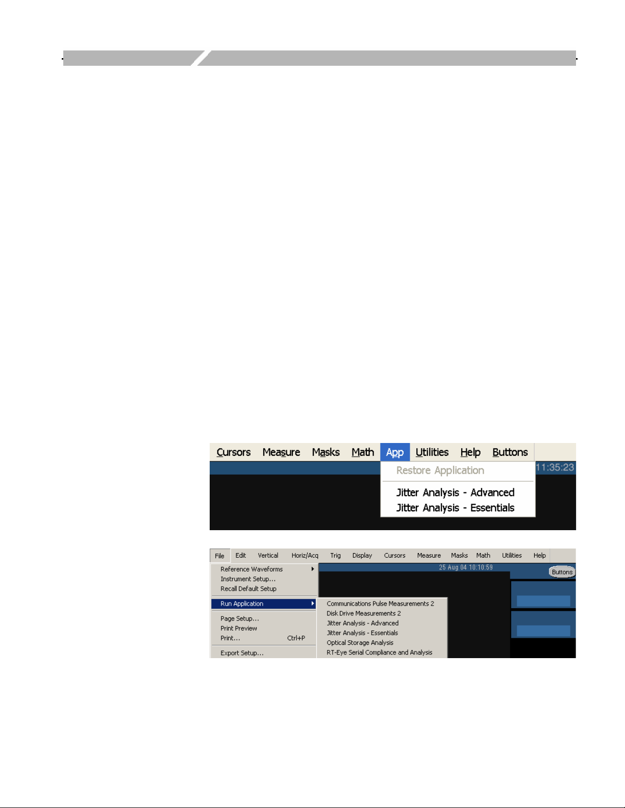
Starting the TDSJIT3 v2 Application

The way you start the application depends on the oscilloscope model. On the oscilloscope menu bar, select App> Jitter Analysis - Advanced or select File> Run Application> Jitter Analysis - Advanced. If you are using the TDSJIT3 v2 Essentials application, select Jitter Analysis - Essentials.

Figure 4: Starting the TDSJIT3 v2 application

TDSJIT3 v2 Jitter Analysis Online Help 5

Operating Basics

Returning to the Application

The way you return to the application depends on the oscilloscope model.

Figure 5: Returning to the application

Minimizing and Maximizing the Application

To minimize the application, select File> Minimize or the command button in the application menu bar. When you minimize the application, the oscilloscope fills the display.

To maximize the application, select

Exiting the Application

To exit the application, select File> Exit or the command button in the application menu bar. When you exit the application, you can choose to keep the oscilloscope setup currently in use with the application or to restore the oscilloscope setup that was present before you started the application.

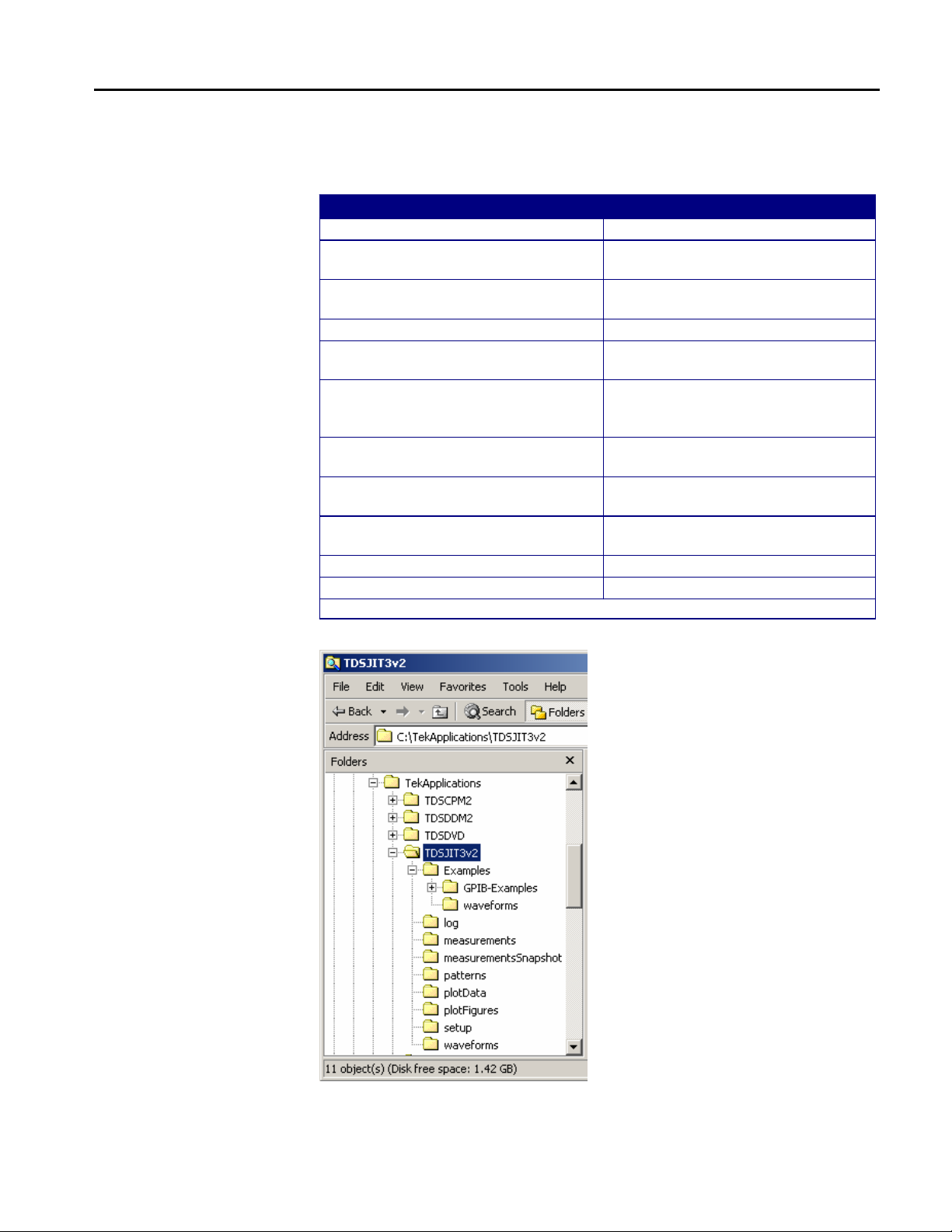
Application Directories and Usage

During installation, the application sets up directories for various functions, such as to save setup files, and uses extensions appended to file names to identify the file types.

in the oscilloscope task bar.

TDSJIT3 v2 Jitter Analysis Online Help

Operating Basic

Table 1: Directories and usage

Default directory names*

\TDSJIT3v2 Home location \TDSJIT3v2\Examples\GPIB-Examples Examples of remote control programs

\TDSJIT3v2\Examples\waveforms Waveform files used in the tutorial

\TDSJIT3v2\log Statistics log files \TDSJIT3v2\measurements Log files of data points for each

\TDSJIT3v2\measurementsSnapshot Measurement log files for the Save

\TDSJIT3v2\patterns Pattern files for the Advanced Clock

\TDSJIT3v2\plotData Data exported from measurement

\TDSJIT3v2\plotFigures Image files exported from

\TDSJIT3v2\setup Setup files \TDSJIT3v2\waveforms Worst case waveforms files

* All subdirectories are located in the C:\TekApplications directory.

Directory use

that use GPIB commands

and application examples

selected measurement

Current Measurements option (Log Measurements)

Recovery configuration

plots

measurement plots

Figure 6: Directory structure

TDSJIT3 v2 Jitter Analysis Online Help

Operating Basics

Table 2: File name extensions

Extension Description

.bmp File that uses a “bitmap” format .csv File that uses a "comma separated value" format .ini TDSJIT3 application setup file .jpg File that uses a “joint photographic experts group” format .mat File that uses native MATLAB binary format .png File that uses a “portable network graphics” format .set Oscilloscope setup file that is recalled with an application .ini file;

.txt File that uses an ASCII format .wfm Waveform file; can be recalled into Reference memory

Tips on the TDSJIT3 v2 User Interface

Here are some tips to help you with the application user interface:

• Use the Jitter Wizard to set up and take one measurement from a set of

commonly used measurements

both files will have the same name

• Select a Source before selecting each measurement

• Select any waveform source and any measurement multiple times to use

different configuration options

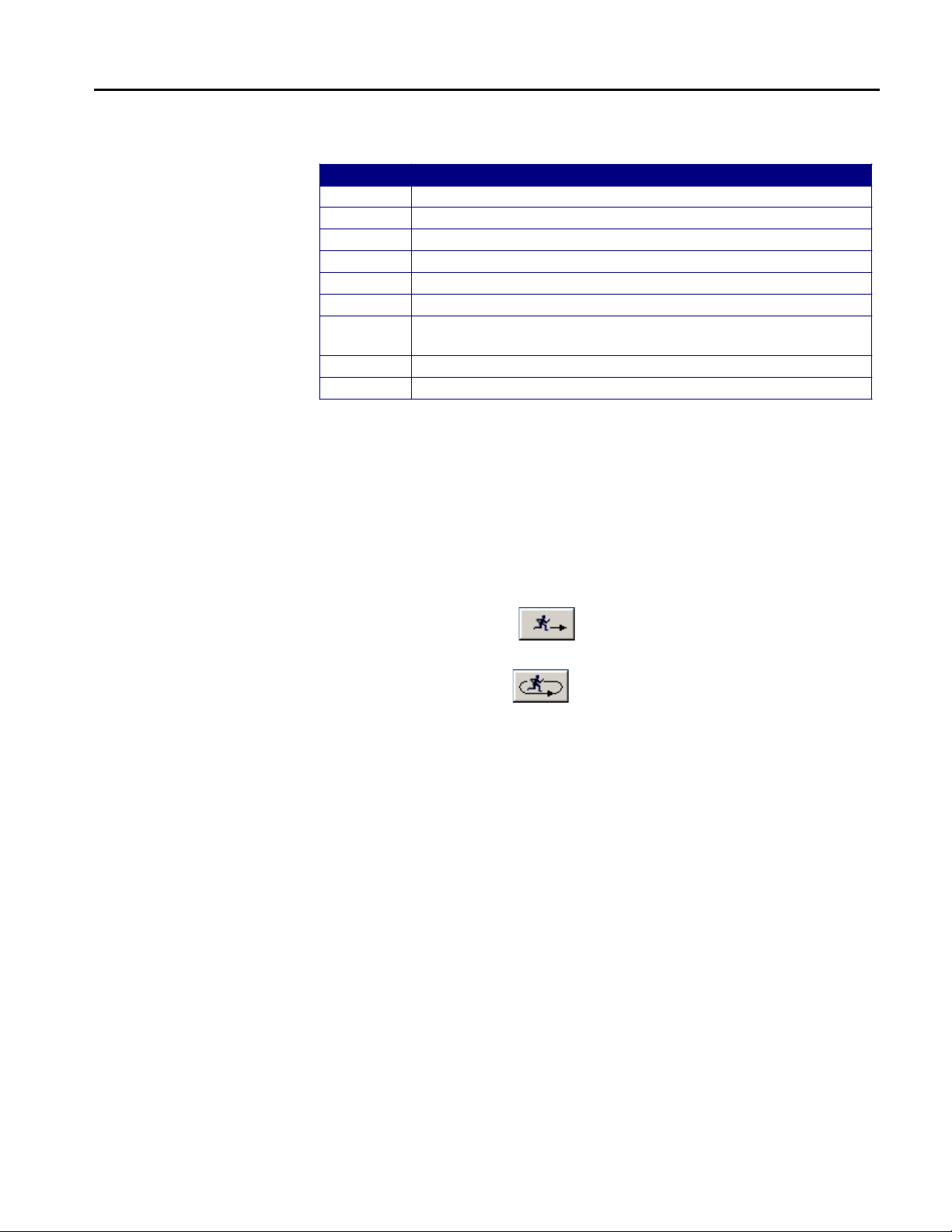
• Use the Single run button

to obtain a single set of measurements from

a single run; push the button again to interrupt the acquisition

• Use the Run/Stop button

to acquire measurements from continuous runs; push the button again to interrupt the current acquisition, or push the Single button to stop sequencing when the current acquisition and measurement cycle is complete

TDSJIT3 v2 Jitter Analysis Online Help

Operating Basic

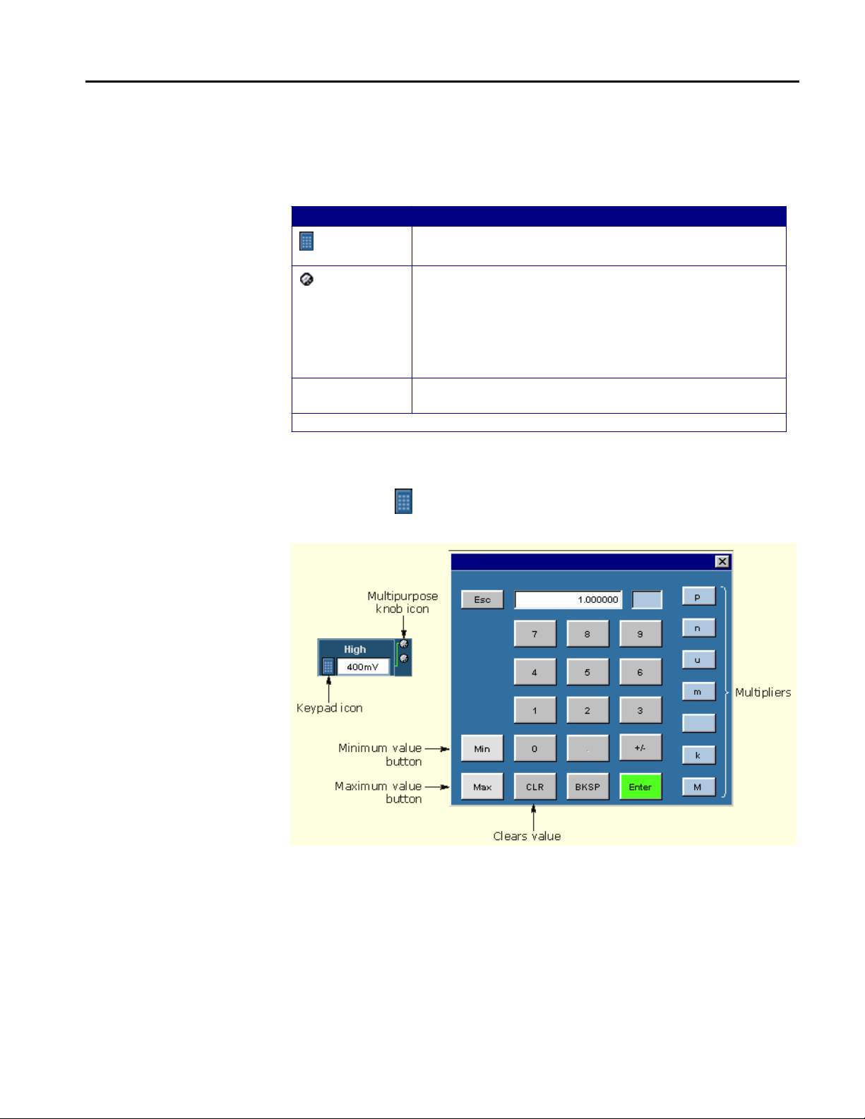
How to Enter Numeric Values

Table 3: Entering numeric values

Method Description

Virtual Keypad

Keypad

Multipurpose

knob*

Edit box*

* When selected twice, the Keypad appears.

Displays the virtual keypad (looks similar to a calculator); use to enter a value

Displays a line between the icon and the option box to indicate that either the upper or lower multipurpose knob on the front panel of the oscilloscope is active; turn the knob to select a value

Press the FINE button on the oscilloscope to enter or select the smallest values or units

Type in a value from the physical keyboard and press the Enter key

Note: Select the icon, and then use the virtual keypad to enter information, such as reference voltage levels.

Figure 7: On-screen keypad

TDSJIT3 v2 Jitter Analysis Online Help

Operating Basics

Using Basic Oscilloscope Functions

You can use oscilloscope controls and functions while the application is running. To do so, select a menu from the oscilloscope Menu bar (or Toolbar) and access menus, or use the front-panel knobs and buttons. You can also use the oscilloscope Help menu to access information about the oscilloscope and how to use it.

When you access some oscilloscope controls, the oscilloscope fills the display.

File Menus

You can use the File menus to save and recall different application setups and recently accessed files.

Do not edit a setup file or recall a file not generated by the application.

Table 4: File menus

Menu/function Description or function

Default Setup Recalls most default (startup) parameters Recall*

Save* Recent Files Select from a list of the four most recently accessed setup

Dock Positions and locks the TDSJIT3 v2 application in the lower

Undock Unlocks and allows you to move the TDSJIT3 v2 application

Minimize Minimizes the application Exit Exits the application; you can choose to retain the current

*Save or Recall functions also save or recall the associated oscilloscope setup file (.set); an oscilloscope file is recalled if the application finds a .set file with a matching name.

Browse to select an application setup (.ini) file to recall; restores the application to the values saved in the setup file

Saves the current application settings in a .ini file

files (saved or recalled) and recall that setup

half of the oscilloscope display and the oscilloscope application in the upper half of the display

to another position in the oscilloscope display or to a second monitor; the oscilloscope display returns to full size

oscilloscope settings or restore the oscilloscope to settings prior to starting the application

Navigating the User Interface

The application provides you with several methods to set up the application:

• The Jitter Wizard

• The Measurement Setup Sequence buttons

• The menus available in the menu bar

TDSJIT3 v2 Jitter Analysis Online Help

Operating Basic

The Jitter Wizard allows you to set up, configure, and launch a single measurement without requiring any knowledge of the control menus. However, it does not provide access to many of the advanced features.

The Measurement Setup Sequence buttons show the logical order you would follow to set up the application if you do not use the Jitter Wizard.

The menus from the menu bar allow the same full control as the Measurement Setup Sequence buttons, but are accessible at all times.

General Steps to Set Up the Application

Jitter Wizard

Figure 8: General steps to set up the application.

The Jitter Wizard provides a quick and easy graphical interface that guides you through a short series of menus so you can take measurements in the fewest steps possible. The wizard lets you pick one measurement from a subset of measurements, and then take a single measurement only. (The application can take six measurements simultaneously.)

The selections you make in each wizard menu determine the subsequent choices the wizard offers in the next selection menu. You can use several methods to configure the wizard: by preference selections, by default selections, or a combination of both.

Note: You can set the Jitter Wizard menu to always appear when you start the application.

To quickly take measurements, follow these steps:

1. Select Measurements> Wizard or select Help> Wizard to launch the Jitter Wizard.

2. Select a measurement category.

3. Select the default settings.

TDSJIT3 v2 Jitter Analysis Online Help

button in each subsequent menu to use all the

Operating Basics

4. Select the

The wizard closes, the application takes the measurement, and displays statistical results.

Note: The statistical results when you use the wizard are identical to the results when you do not use the wizard if the measurement and setup are the same.

When you are through setting up a measurement and plots with the wizard, select the Run button. The application takes the measurement and displays the results,

including selected plots. To obtain new measurement results, select the Single Run button.

If you select the Cancel button, the wizard exits and discards all of the selections.

Note: After you use the wizard, you may decide to refine some options, such as the calculated values for reference voltage levels, to suit your analysis situation.

Note: The application does not launch the Jitter Wizard when you start the application if you clear the Show This Wizard At Startup option.

button.

Figure 9: Jitter Wizard when launched

TDSJIT3 v2 Jitter Analysis Online Help

Operating Basic

User Interface Information

The application uses a Microsoft Windows based user interface. Display the definitions of the application user interface items, or view a menu labeled with the user interface items.

Note: The oscilloscope application shrinks to half size and appears in the top half of the screen when the application is running.

Table 5: User interface items

Item Description

Area Visual frame that encloses a set of related options Box Use to define an option; enter a value with the Keypad or

a Multipurpose knob

Browse Displays a window where you can look through a list of

directories and files Button Use to define an option; not a command button Check box Use to select or clear an option Command button Initiates an immediate action, such as the Start command

button in the Control panel Control panel Located to the right of the application; contains command

buttons that you use often, such as to Start sequencing Keypad On-screen keypad that you can use to enter numeric

values List box Use to select an option from a list Menu All options in the application window (except the Control

panel) that display when you select a menu bar item Menu bar Located along the top of the application display and

contains application menus Multipurpose

knob

Option Any named button (other than a command button) or any

Status bar Line located at the bottom of the application display that

Tab Short cut to a menu in the menu bar or a category of

Virtual keyboard On-screen keyboard that you can use to enter

Scroll bar Vertical or horizontal bar at the side or bottom of a

Icon that indicates when you can use one of the

multipurpose knobs on the oscilloscope front panel to

adjust a value

named box that defines a control or task

shows the name of the current menu (location) and the

latest Warning or Error message

menu options; most tabs are short cuts

alphanumeric strings, such as for file names

display area that you use to move around in that area

TDSJIT3 v2 Jitter Analysis Online Help

Operating Basics

Figure 10: Menu with user interface items

Figure 11: Menu navigation tree

TDSJIT3 v2 Jitter Analysis Online Help

Operating Basic

Setting Up the Application for Analysis

The Measurement Setup Sequence buttons show the logical order you would follow to set up the application if you do not use the Jitter Wizard. The menus from the menu bar allow the same full control as the Measurement Setup Sequence buttons, but are accessible at all times.

When you use the Measurement Setup Sequence buttons or the menus, you may need to perform some or all of the following tasks:

• Select up to six measurements

• Configure measurement options

• Configure waveform sources, such as the Source Autoset function

• Create and configure up to four plots

• Log statistics, measurements, or worst case waveforms

• Take measurements and display the results

Selecting Measurements

After setting up the application, you can select the button to take measurements. The application displays the results as statistics, and as plots if you set up the Plot Create menu.

After taking measurements, you can do any of the following tasks:

• View the results as statistics

• View the results graphically

You can use the Measurements Select menu to select up to six measurements. You can always access the menu by selecting Measurements> Select in the menu

bar. In addition, you can use the the Measurements Select menus.

To select a measurement, always choose the Source (or sources) first, and then select a measurement. To select a measurement, follow these steps:

1. Select the Source in the Select Source area.

2. Select a measurement in the Add Measurement area.

3. For some advanced configurations, use the options in the Math Defs area in conjunction with the Source Select area.

You can select the same measurement type multiple times using different sources. To do so, select a source first, and then select a measurement. You can also create two or more measurement entries that use the same measurement type and source, and then configure each measurement differently.

button (when visible) as a short cut to

or command

TDSJIT3 v2 Jitter Analysis Online Help

Operating Basics

You can view the configured measurements, sources, and any associated values in various Measurement Summary menus.

Figure 12: Measurements Select menu

Select Source Area

The application takes measurements from waveforms specified as sources (also called input sources). You can select a live channel (CH1, CH2, CH3, or CH4), a reference (Ref1, Ref2, Ref3, or Ref4), or a math (Math1, Math2, Math3, or Math4) waveform as a source.

The titles above the Select Source option list boxes vary depending on the measurement category.

Note: Most measurements require one source. The Setup, Hold, Clock-to-Output, Skew, and Crossover Voltage (TDSJIT3 v2 Advanced only) measurements require two sources.

Option names (in the Select Source area) vary with the category of measurements.

Clock Data Clk-Data General

Figure 13: Select Source options by measurement category

TDSJIT3 v2 Jitter Analysis Online Help

Operating Basic

Table 6: Measurement definitions

Area Option Description

Clock Period Elapsed time between consecutive crossings of the mid

reference voltage level by the waveform in the specific

direction; see the Common Cycle Start Edge option Frequency Inverse of the period for each clock cycle TIE Difference in time between each edge of a designated

polarity on a sampled clock waveform to the

corresponding edge on a calculated clock waveform with

a constant frequency (zero jitter) PLL TIE Measurement errors relative to a timing reference that is

recovered from a data stream by a phase locked loop

(PLL); for TDSJIT3 v2 Advanced only Cycle-Cycle Difference in period measurements from one cycle to the

next N-Cycle Difference in elapsed time between two consecutive

groups of N-Cycles where N is a configuration object that

you can set Positive Cy-Cy

Duty Negative Cy-Cy

Duty Positive Duty

Cycle Negative Duty

Cycle

Data Period Elapsed time between when a waveform crosses specific

Frequency Inverse of the period for each data cycle TIE Difference in time between the data edges on an

PLL TIE Measurement errors relative to a timing reference that is

Clk-Data Setup Elapsed time between when a data waveform crosses a

Hold Elapsed time between when the clock waveform crosses

Clk-Out Elapsed time between when the clock waveform crosses

Difference between two consecutive positive widths

Difference between two consecutive negative widths

Ratio of the positive portion of the cycle relative to the

period

Ratio of the negative portion of the cycle relative to the

period

reference voltage levels in the opposite direction once

acquired data waveform to the data edges on a

recovered data waveform with a constant rate (zero jitter)

recovered from a data stream by a phase locked loop

(PLL); for TDSJIT3 v2 Advanced only

voltage reference level followed by the clock signal

crossing its own voltage level

a voltage reference level followed by a data waveform

crossing its own voltage level

a voltage reference level followed by an output waveform

crossing its own voltage level

TDSJIT3 v2 Jitter Analysis Online Help

Operating Basics

Table 7: General measurement definitions

Area Option Description

General Rise Time Time difference between when the Lo reference level is

crossed and the Hi reference level is crossed on the rising edge of the waveform

Fall Time Time difference between when the Hi reference level is

crossed and the Lo reference level is crossed o n the falling edge of the waveform

Positive Width Amount of time the waveform remains above the mid

reference voltage level

Negative Width Amount of time the waveform remains below the mid

reference voltage level

High Time Amount of time the waveform remains above the high

reference voltage level

Low Time Amount of time the waveform remains below the high

reference voltage level

Skew Difference in time between two similar edges on two

waveforms with the assumption that every edge in one waveform has a corresponding edge (either the same or opposite polarity) in the other waveform; edge locations are referenced to the mid reference voltage level

Crossover Voltage

Edge timing derived from the crossover (voltage) of differential clock or data measurements; for TDSJIT3 v2 Advanced only

Math Definitions

The application includes four preset math operations and an option to use any other math operation as defined in the oscilloscope. You can assign each math waveform (Math1, Math2, Math3, or Math4) to any of these five operations.

The Math Defs area includes the following preset math operations:

• Ch1-Ch3

• Ch2-Ch4

• Ref1-Ref2

• Ref3-Ref4

You can select Scope User if you want to use a math waveform based on a userdefined math operation. To define your own math operation, use the oscilloscope math equation editor.

TDSJIT3 v2 Jitter Analysis Online Help

Operating Basic

Clearing Measurements

You can remove individual or all selected measurements through the Measurements Select menu. To remove an individual measurement, follow these steps:

1. Select the measurement to be removed in the table on the right side of the Measurements Select menu.

Configuring a Measurement

2. Select the

3. To remove all selected measurements, select the

button.

Most measurements offer configuration options. The options available in each Configure Measurement menu are specific to the selected measurement.

You can always access the menus by selecting Measurements> Configure in the

menu bar. In addition, you can use the

button (when visible) as a short

cut to the Configure Measurements menus.

The application includes the following Configure Measurement menus:

• General

• Clock Recovery

• Filters (TDSJIT3 v2 Advanced only)

Configure Measurement Menus Definitions

Table 8: File menus

Menu name Description

General Define waveform edges; define range limits for some

measurements

Clock Recovery Define reference clock frequency or PLL loop bandwidth for

some measurements; advanced functions

Filters*

* TDSJIT3 v2 Advanced only.

Define high pass, low pass, or band pass filters; advanced functions

TDSJIT3 v2 Jitter Analysis Online Help

Operating Basics

Table 9: Configure Measurement menus and applicable measurements

Measurements General Clock recovery Filters*

Clock TIE Clock PLL TIE*

Data TIE Data PLL TIE*

Clock Period Clock Frequency

Data Period Data Fre quency

Cycle-Cycle N-Cycle Positive Duty Cycle Negative Duty Cycle Setup Hold Clk-Out Skew Crossover Voltage*

Positive Cy-Cy Duty Negative Cy-Cy Duty Rise Time Fall Time Positive Width Negative Width High Time Low Time

* TDSJIT3 v2 Advanced on ly. ** TIE: RjDj configure options are for TDSJIT3 v2 Advanced only. † No configuration options are available for these measurements.

Yes** Yes Yes

Yes - - - Yes

- - - Yes Yes

Yes - - - - - -

None†

General

You can select which waveform edge the application will use to take measurements. The name of the edge option depends on the measurement being configured.

Edge options appear in the General Configure Measurement menu. Some measurements include two edge options because they require two waveforms.

Note: Data measurements do not include Waveform Edge options.

TDSJIT3 v2 Jitter Analysis Online Help

Operating Basic

Clock Edge Options

The Clock Edge option defines which edge of the clock input is used to calculate the statistics of clock based measurements.

Figure 14: Clock edge options

Active Edge Options

The Active Edge option defines which edge of the source waveform is used to take measurements.

Figure 15: Active edge options

TDSJIT3 v2 Jitter Analysis Online Help

Operating Basics

Clock and Data Edge Options

The Clock Edge option defines which edge of the clock input is used to calculate the statistics of clock based measurements. The Data Edge defines which edge of the data input is used to calculate the statistics on clock-data based measurements.

Figure 16: Clock and Data edge options

From Edge and To Edge Options

The From Edge option defines which edge on the first waveform is used to take the measurement. The To Edge option defines which edge on the second waveform is used to take the measurement, the same edge or the opposite edge as the first waveform.

Figure 17: From Edge and To Edge options

TDSJIT3 v2 Jitter Analysis Online Help

Operating Basic

Main Edge Options

The Main Edge option defines which edge on the Main waveform is used to take the measurement.

Figure 18: Main edge options

Measurement Range Limits Configuration

For two-channel measurements, you can specify the minimum and maximum range of valid measurement values. Individual measurements falling outside the selected range are discarded.

The default values for the Meas Range Limits options vary by measurement.

Figure 19: Meas Range Limits options

N-Cycle Measurement Configuration

You can define a Clock Edge and some unique General Configuration options for the N-Cycle measurement.

TDSJIT3 v2 Jitter Analysis Online Help

Operating Basics

Table 10: N-Cycle measurement configuration

Option Description

Clock Edge Waveform edge used to calculate statistics N= Number of cycles in an N-cycle group 1st Meas: Start @ Edge Number of cycles skipped prior to starting the

measurement

Edge Increment

1 N

N-Cycle Measurement Options

Specifies how consecutive measurements (each spanning 2 N-cycles) jump forward

By one cycle in the waveform By N cycles in the waveform

Figure 20: N-Cycle measurement options

TIE Rj/Dj

Rj/Dj analysis refers to the process of separating jitter into the major categories of Random Jitter (Rj) and Deterministic Jitter (Dj), and further separating Dj into specific subcomponents based on observable properties of the jitter. This can help you understand and reduce the jitter in your circuit. For serial data signals with embedded clocks, it also allows you to accurately predict the eye opening and total jitter at very low bit error rates, in a few seconds. By contrast, direct measurement of these quantities can take hours for a single eye-opening measurement.

For data signals, there are two methods of Rj/Dj analysis provided in the application. The Rj/Dj Analysis of Repeating Patterns Using a Spectral Approach, which requires a data signal with a cyclically repeating data pattern, is a method of analysis with wide industry acceptance. The Rj/Dj Analysis of Arbitrary Patterns method uses a technique that allows jitter separation and analysis even if the data pattern is random or unknown.

Each method has advantages and limitations. For clock signals, the spectral analysis approach is automatically used.

TDSJIT3 v2 Jitter Analysis Online Help

Operating Basic

Once an Rj/Dj analysis has been done, the results may be plotted in the form of a Bathtub Plot.

Rj/Dj Analysis of Repeating Patterns Using a Spectral Approach

This method of Rj/Dj analysis uses a Fourier transform of the time-interval error signal to identify and separate jitter components. It is described in the Fibre Channel -- Methodologies for Jitter and Signal Quality Specification (MJSQ), and was the analysis method originally introduced with the TDSJIT3 application.

This method requires that the data signal be composed of a pattern of N bits that are repeated over and over. The pattern length (N) must be known, although it is not necessary to know the specific bits that make up the pattern.

When the data pattern is not repeating, or is unknown, a second method of Rj/Dj analysis may be used. (It may also be used if the pattern is repeating, and correlates well with the Spectral method in this case.) This method assumes that the effects of Intersymbol Interference (ISI) only last for a few bits. For example, in a band-limited link where a string of ones follows a string of zeros, the signal may require three or four bit periods to fully settle to the "high" state.

In this method, an analysis window with a width of K bits is slid along the waveform. For each position of the window, the time interval error of the rightmost bit in the window is stored, along with the K-1 bit pattern that preceded it. After the window has been slid across all positions, it is possible to calculate the component of the jitter that is correlated with each observed K-1 bit pattern, by averaging together all the observed errors associated with that specific pattern.

In the configuration menu for the arbitrary-pattern method, the Window Length field allows you to select how many bits are included in the sliding window. The window should include enough bits to encompass the impulse response of the system under test, usually 5 to 10 bits. A good practical test is to check whether increasing the window length causes any appreciable change in the jitter results; if not, the window length is effectively capturing all the ISI effects. The disadvantage of increasing the window length is that it uses more memory and slows the processing.

The configuration menu also includes a field for selecting what population of each K-1 bit pattern must be accumulated before the TIE associated with that pattern is considered accurate. Using a larger population means that more observations are averaged together, so that the variance of the measurement is reduced. Specifying a larger population has the disadvantage of requiring a longer measurement period before results can be calculated.

It may be necessary to sequence the instrument several times before enough statistics are accumulated to provide results. A vertical gauge on the TIE:RjDj results screen provides an indication of how the accumulation is progressing.

The arbitrary-pattern approach to measuring jitter may not be appropriate if there are very-long-duration memory effects in your data link. An example would be if there is impedance mismatch reflections that arrive long enough after the initial edge to fall outside the analysis window.

TDSJIT3 v2 Jitter Analysis Online Help

Operating Basics

Bathtub Curve and BER Versus Decision Time

The Bathtub Curve plot shows the eye opening and total jitter values as functions of the BER level. The plot is obtained from the Rj/Dj separation.

Figure 21: Bathtub Curve and BER versus Decision Time

Table 11: TIE: RjDj analysis configuration

Option Description

Separation Enables or disables Rj/Dj separation analysis Total Jitter

BER=1E- ? Sets the BER level for the eye opening and total jitter Dat a Patt ern* T ype* Selects a Repeating or an Arbitrary data pattern Pattern Length* When the Type option is set to Repeating, sets the

pattern length of the repetitive pattern data; use for spectrum analysis Rj/Dj separation

Window Length* When the Type option is set to Arbitrary, sets the pattern

window length used for arbitrary pattern Rj/Dj separation

Population* When the Type option is set to Arbitrary, sets the

minimum population limit for each pattern to be qualified for arbitrary pattern Rj/Dj separation

* Available only for Data TIE and Data PLL TIE measurements.

TDSJIT3 v2 Jitter Analysis Online Help

Operating Basic

Figure 22: TIE: RjDj analysis options for Clock TIE and Clock PLL TIE

Figure 23: TIE: RjDj analysis options for Data TIE and Data PLL TIE

Clock Recovery Configuration

For waveforms that are synchronized to a nominal clock frequency, TIE measurements offer a choice of clock recovery methods. Clock recovery is defined as the way in which the TDSJIT3 v2 application determines the theoretically jitter-free clock to which the waveform will be compared.

Constant (straight line) clock recovery is implicitly chosen by selecting a Clock TIE or Data TIE measurement. Phase-Locked Loop clock recovery is chosen by selecting a Clock PLL TIE or Data PLL TIE measurement.

For Data measurements (Data Period, Data Frequency, Data TIE, and Data PLL TIE) on signals with extremely high jitter, advanced clock recovery support is offered. This support is not needed or recommended for most signals. It allows you to provide extra guidance to the clock recovery algorithm with respect to how many unit intervals are represented by each pair of clock edges. This is most useful in cases where the total jitter on a data signal exceeds 0.5 unit intervals.

TDSJIT3 v2 Jitter Analysis Online Help

Operating Basics

In Constant Clock Recovery, the clock is assumed to be of the form A*sin(2 ft + ), where the frequency (f) and phase ( ) are treated as unknown constants. Once a source waveform has been acquired and the edges extracted, f and are chosen using linear regression, so that the recovered clock minimizes the meansquared sum of the Time Interval Error (TIE) for that waveform.

Figure 24: Constant Clock Recovery concept

Constant Clock Recovery Setup

The Ref Clock Frequency control area provides three options that control how the clock recovery is performed.

Selecting Autocalc Every Acq will allow the clock-recovery algorithm to choose a new best-fit clock frequency and phase for each new oscilloscope acquisition.

Selecting Autocalc 1st Acq will allow the clock-recovery algorithm to choose a new best-fit clock frequency and phase only on the first acquisition. Subsequent acquisitions will choose a best fit on clock phase but retain the clock frequency found on the first acquisition. Clearing the measurements by choosing Clear on the control panel will reset the clock recovery so that both frequency and phase are optimized on the subsequent acquisition.

Selecting Custom allows you to specify an exact clock frequency, so that absolutely no clock frequency optimization is performed. A best fit of the clock phase is still performed on every acquisition.

Table 12: Reference Clock Frequency configuration

Option Description

Autocalc 1st Acq Calc ulates the best fit of the initial acquisition or the

first acquisition after clearing results, and then uses the

value until yo u clear the results Autocalc Every Acq Calculates the best fit for each acquisition (default) Custom: Value Uses the exact frequency you enter

TDSJIT3 v2 Jitter Analysis Online Help

Operating Basic

Figure 25: Reference Clock Frequency options

Phase-Locked Loop (PLL) Clock Recovery

In PLL Clock Recovery, the application simulates the behavior of a hardware phase-locked loop clock recovery circuit. This is a feedback loop in which a voltage-controlled oscillator is used to track, or follow, slow variations in the bit rate of the input waveform. Such loops are frequently used to recover the clock in communications links that do not transmit the clock as a separate signal. The PLL parameters in the application may be adjusted to mimic the behavior of a receiver in such a link, within certain guidelines.

Figure 26: Phase-Locked Loop (PLL) Clock Recovery concept

PLL Clock Recovery Setup

The PLL control area provides control over the phase-locked loop used for clock recovery. You can choose the loop bandwidth and the loop order, and if a second-order loop is chosen, you can specify the damping factor.

The loop bandwidth can be selected implicitly by specifying a data communications standard, or it can be set explicitly.

To use a standards-based setup, select the Standard Frequency button. From the Standard: Speed (Gb/s) list box, choose the standard that matches your data link. For example, choose "FC2125: 2.125" to test a 2.125 Gbit/second Fibre Channel link. The PLL bandwidth will be set to 1/1667 of the baud rate.

TDSJIT3 v2 Jitter Analysis Online Help

Operating Basics

To manually control the loop bandwidth, choose the User button and use the Value option to select the 3 dB bandwidth of the loop, in Hertz.

You can use the PLL Order list box to choose between a first-order or secondorder loop. More correctly, this is the loop type, where a type 1 loop has a transfer function that approaches zero frequency with a slope of 1/s and a type 2

1 s

loop approaches zero frequency with a

slope. The term Order is used in the application as a concession to popular usage. For a more thorough treatment of loop type and order, see Frequency Synthesis by Phase Lock, by William Egan.

If you choose a second-order loop, the Damping option becomes enabled. (The Damping Factor does not apply to first-order loops.)

Note: Although it is possible to configure a second-order PLL with a bandwidth up to 1/10 of the baud rate, such a loop will have poor dynamic performance. This is because second-order loops have less phase margin than first-order loops. A preferred alternative to using a second-order PLL with a high bandwidth is to use a second-order high-pass measurement filter to emulate the effects of the PLL.

Table 13: PLL Loop Bandwidth configuration

Option Description

Standard Frequency

Custom: Value Sets the 3 dB bandwidth of the Phase Locked Loop (PLL) PLL Order Sets the or der of the PLL Damping Sets the damping ratio of the PLL Advanced*

* Available only for Data PLL TIE measurements.

Loop BW Options

Select a standard: FC133:0.1328, FC266:0.2656, FC531:1.0625, FC1063:11.063,: FC2125:2.125, IB2500:2.5, SerATAG1:1.5, SerATAG2:3, SerATAG3:6, USB_FS:0.12, USB_H S:0.48, 1394b_S400b:0.4915, 1394b_S800b:0.983, 1394b_S1600b:1.966, GB_Ethernet:1.25, 100BaseT:0.125, OC1:0.0518, OC3:0.155, OC12:0.622, OC48:2.488

Figure 27: PLL Loop Bandwidth options

TDSJIT3 v2 Jitter Analysis Online Help

Operating Basic

Advanced Clock Recovery Setup

For Data Period, Data Frequency, Data TIE and Data PLL TIE measurements, you may use several types of advanced clock recovery if needed. The advanced clock recovery tools can be helpful if your signal has jitter excursions that exceed

0.5 unit intervals, by guiding the application in choosing the number of unit intervals that correspond to each pair of edges. Advanced clock recovery is seldom required, and is not recommended for general analysis.

When Advanced Clock Recovery is enabled for a given source, it applies to all Data measurements using that source. For example, if you have Data Period and Data TIE measurements on Channel 1, enabling advanced clock recovery for one measurement will cause it to be enabled for the other as well.

Two types of advanced clock recovery are available. In the first, you can provide the nominal data rate to the clock recovery algorithm. Normally, the application analyzes your data and determines the nominal data rate automatically. If you know the data rate or unit interval to an accuracy of +/- 3%, you can provide this information as a clue to the algorithm.

You can also provide clock recovery guidance in the form of a known data pattern. The pattern is specified by using an ASCII text file containing the characters 1 and 0. The file may contain other characters, spaces and tabs for formatting purposes, but they will be ignored. Several files for commonly-used patterns are included with the application, and you may use these as examples if you wish to create your own pattern files. The default location for pattern files is C:\TekApplications\TDSJIT3v2\patterns.

If you use pattern file guidance, the clock recovery algorithm will perform a best fit of the selected data pattern against the acquired edge sequence. It will then use the pattern file to determine the number of unit intervals that fall between each set of edges.

Note: Clock recovery using pattern match will provide erroneous results if your data has missing edges or extra edges at the defined edge threshold.

Table 14: Advanced Clock Recovery configuration

Area/option Description

Nominal Data Rate On Off Enables or disables advanced clock recovery through

rate guidance Unit Interval Defines the nominal data r ate by UI in time Bit Rate Defines the nominal data rate by the bit rate in

frequency Known Data Pattern On Off Enables or disables advanced clock recovery through a

known data pattern Pattern File Name Selects a file to use for the data pattern OK button Accepts changes and closes Cancel button Discards changes and closes

TDSJIT3 v2 Jitter Analysis Online Help

Operating Basics

Figure 28: Advanced Clock Recovery options

Filters

For some measurements (Clock Period, Clock Frequency, Clock TIE, Clock PLL TIE, Data Period, Data Frequency, Data TIE, and Data PLL TIE), the measurements-versus-time waveform (time trend) that is derived from the original oscilloscope waveform can be filtered before it is passed to the statistics and plotting subsystems.

Figure 29: Optional filters

You can modify the time trend by applying filters that block specific frequency bands. You can configure a High Pass filter to block out the low frequency band or a Low Pass filter to block out the high frequency band.

TDSJIT3 v2 Jitter Analysis Online Help

Operating Basic

Figure 30: Filter characteristics

Band Pass Filtering

You can create a band pass filter by enabling both the High Pass and Low Pass filters on a measurement. The cutoff frequency for the Low Pass filter must be greater than or equal to the cutoff frequency for the High Pass filter.

You should be aware that setting the cutoff frequencies close to each other may effectively filter out all of the time trend, or all but a small amount of noise. This diagram shows the spectrum of the time trend passed to the statistics and plotting subsystems when you use both the High Pass and the Low Pass filters.

Figure 31: Band Pass filtering

Influence of High Pass Filters on Period and Frequency Statistics

TDSJIT3 v2 Jitter Analysis Online Help

Operating Basics

High-pass filters attenuate low frequencies, and filter out DC values entirely. When a high-pass filter is added to a period or frequency measurement, the mean value of the filtered measurement goes to zero. This can be seen by creating a Time Trend plot of a high-pass-filtered period or frequency measurement. Although this is the correct theoretical behavior for the filtered measurement, it isn't very useful if the Results panel reports that the mean period or frequency is zero. For this reason, the mean values that appear in the results panels for Period and Frequency measurements are the values prior to the filter.

Table 15: Filters configuration

Option Description

High Pass Filter Spec When enabled, blocks the low frequency band and

passes on only the high frequency band of the

waveform; defined as 1st order, 2nd order, or 3rd order

Butterworth Freq (F1)* High Pass filter cutoff frequency; frequency at which

the filter magnitude has dropped by 3 dB Low Pass Filter Spec When enabled, blocks the high frequency band and

passes on only the low frequency band of the

waveform; defined as 1st order, 2nd order, or 3rd order

Butterworth Freq (F2)* Low Pass filter cutoff frequency; frequency at which the

filter magnitude has dropped by 3 dB

* Includes a 3 dB attenuation.

These options are also available for Data measurements.

Figure 32: Filters options

TDSJIT3 v2 Jitter Analysis Online Help

Operating Basic

Advanced Filter Configuration

The measurement filters are implemented using infinite impulse response (IIR) designs. As with any causal filter, a transient may occur at the filter’s output in response to the arrival of the input signal. It is usually desirable to exclude this transient from the measurement results.

In the TDSJIT3 v2 application, the filter transient is managed by specifying a settling time, Td. A smoothing window ramps the filter input from 0 to 1 during this settling time. The output of the filter during the settling time is excluded from the measurement results. The smoothing window has a raised-cosine profile which is described by:



)(





where the settling time of the filter (Td) is configurable. The operation of the smoothing window is shown graphically in the Effect of the Smoothing Window topic.

By default, the settling time is set to 2/Fc, where Fc is the lowest filter cut-off frequency applied to the measurement.

Note: Setting the settling time to less than 1/Fc increases the chance that the measurement results will include effects that are due to the filter transient. The user interface will warn you if you configure the measurement this way.

Table 16: Advanced Filter configuration

Option Description

Duration D efines the amount of time excluded from the measurement

OK button Accepts changes and closes

 

−=

cos1

 

results to allow the filter to settle





⋅

ttWπ











for

Tt <≤0

Figure 33: Advanced Filter options

TDSJIT3 v2 Jitter Analysis Online Help

Operating Basics

Configuring Sources

Figure 34: Effect of the Smoothing window

You may configure the sources associated with your measurements, which can be as simple as using the Autoset features that automatically calculate the scale or the reference voltage levels.

You can always access the menus by selecting Measurements> Source in the

menu bar. In addition, you can use the cut to the Configure Measurements menus.

The application includes the following Configure Source menus:

• Autoset

• Gate/Qualify

• Ref Levels

• Stat Pop Limit

button (when visible) as a short

TDSJIT3 v2 Jitter Analysis Online Help

Operating Basic

Table 17: Configure Sources menus

Menu name Description

Sources Autoset*

Gate/Qualify*

Ref Levels Specifies reference voltage levels for each measurement

Stat Pop Limit**

* All sources must have the same Horizontal Sample Rate, Record Length, and Position to assure that measurements function properly.

** In Free Run mode, sequencing stops when all the population limits are met.

Automatically changes the vertical scale or horizontal resolution of the measurement source waveforms

Autoset acts on all active (Ch1, Ch2, Ch3, Ch4) sources used by measurements directly or contained in a math source definition

Accurate measurement results require sufficient vertical and horizontal resolution

Gating limits measurements to an area of the source waveform bounded on the left and right by vertical cursors or by the lowest zoom that is on

Qualify limits measurements to the one or more areas of the waveform where a qualifier waveform is active

source; separate reference levels apply to rising and falling edges

Sets the maximum population of all measurements; Free Run sequencing mode will stop when all measurements have attained this limit

Autosetting Sources for Live (Channel) Waveforms

In most situations, you can improve accuracy on channel or math waveform by using the Source Autoset options to optimize the vertical scale or horizontal resolution settings of the oscilloscope.

The Vertical Scale option automatically checks the Peak-to-Peak level of live sources. The vertical scale and offset of all signals with a Peak-to-Peak less than 6 divisions is adjusted so the Peak-to-Peak will be 8 divisions. If the maximum or minimum value of a signal is "clipped," the vertical scale and offset is adjusted so the Peak-to-Peak will be 8 divisions.

The Horizontal Resolution option automatically checks the number of samples/edge on the rising and falling transitions (Rise Time/Resolution and Fall Time/Resolution) of all live channels. The oscilloscope horizontal resolution is set to the largest value that does not cause the samples/edge of the fastest edge to fall below the specified target. The target is 5 samples per edge when optimized for edge resolution, and 2.5 samples per edge when optimized for edge count. Horizontal Resolution sets the acquisition sampling mode to Interpolated Real Time for signals with very high edge speeds. The default record length is 500 k points.

TDSJIT3 v2 Jitter Analysis Online Help

Operating Basics

To automatically define both the vertical and horizontal settings for all channel sources, select the All button. The All option also applies an oscilloscope Autoset on each channel prior to performing the vertical scale and horizontal resolution autoset.

To automatically define the vertical or horizontal settings for active sources, follow these steps:

1. Ensure that any channel waveform that you want to autoset is visible on the oscilloscope.

2. If you intend to select the All or Horizontal Resolution button, configure the Optimize Horizontal For option to one of the following:

• Edge Resolution: results in 5 samples per edge or more, giving you better

edge timing and measurement accuracy.

• High Edge Count: results in as few as 2.5 samples per edge. Some edge

timing accuracy is sacrificed for more edges in a given record length. High edge count is desirable for RjDj analysis in oscilloscopes without extended record lengths.

3. Select one of the following options:

• All button to Autoset both vertical and horizontal setting

• Vertical Scale button to Autoset oscilloscope vertical settings only

• Horizontal Resolution button to Autoset oscilloscope horizontal settings

only

Optionally, select the Undo button to return the oscilloscope to its state prior to autoset.

Note: At rise times less than 100 ps, the application may have only two actual sample points per edge to work with. The application will set up a suitable level of oscilloscope acquisition interpolation to increase the point count per edge to around 5 points.

Table 18: Configure Sources Autoset configuration

Option Description

All Performs a sequence: oscilloscope AUTOSET, Vertical

Scale, and Horizontal Resolution

Vertical Scale If a channel waveform does not exceed six vertical

divisions, decreases the scale so the waveform occupies about 8 divisions

Horizontal Resolution Sets the horizontal resolution so that the number of

samples on the fastest transition (edge) exceeds a specified target; see Optimize Horizontal For option

Undo Returns to the settings present before an Autoset was

performed; disabled after measurements are taken until you perform another Source Autoset

TDSJIT3 v2 Jitter Analysis Online Help

Operating Basic

Table 19: Optimize Horizontal For configuration

Area/option Description

Optimize Horizontal For Edge Resolution Sets the horizontal scale to ? 5 samples per

transition; edge timing accuracy does not improve significantly at higher resolution

Edge timing accuracy will not significantly improve at higher resolution (default)

Max Edge Count Sets the horizontal scale to ? 2.5 samples per

transition; Rj/Dj analysis requires a larger data set If the oscilloscope does not have a long acquisition

memory, it may be necessary to trade some Edge timing accuracy for a larger data set

Figure 35: Configure Sources Autoset options

Gate/Qualify

Gating allows you to limit the analysis to a specific area of the waveform bounded by cursors or zoom limits, thereby excluding unnecessary information. To access the Gating menu, select Measurements> Configure Source> Source Gate/Qualify. View the Configure Sources Gate/Qualify menu.

You can set up a gated region in one of the following ways:

• Zoom

• Cursors (vertical)

Qualifiers allow you to limit the application to more narrowly defined conditions before taking measurements. This is another way to exclude unnecessary information. All sources for the measurements and Qualify input must have the same Horizontal Sample Rate, Record Length, and Position to ensure that measurements function properly. For TIE and PLL TIE measurements, only the first qualified region will be measured even if multiple qualified regions are present.

TDSJIT3 v2 Jitter Analysis Online Help

Operating Basics

Table 20: Configure Sources Gating configuration

Option Description

Off No gating occurs; application takes measurements over the entire

waveform

Zoom Zoom to a specified region of the source waveform and take

measurements within the selected area

Cursors Use oscilloscope cursors to define a specific part of the waveform

and take measurements within the selected area

Configure Sources Gate/Qualify Menu

Figure 36: Configure Sources Gating options

Table 21: Configure Sources Qualify configuration

Option Description

Source*

Mid Shows the vertical reference level of the qualifier waveform Hysteresis Shows the vertical reference margin of the qualifier waveform Active

Off Disables the use of the qualify waveform High

Low

* Measurement and Qualify sources must have the same Horizontal Sample Rate, Record Length, and Position to ensure that measurements function properly.

** For TIE and PLL TIE measurements, only the first qualified region will be measured even if multiple qualified regions are present.

Selects a waveform to qualify the signal or clock source used for the measurement

Enables measurements in regions** where the qualifier waveform exceeds the mid reference level

Enables measurements in regions** where the qualifier waveform falls below the mid reference level

TDSJIT3 v2 Jitter Analysis Online Help

Operating Basic

Ref Levels

Timing measurements are based on state transition times. By definition, edges occur when a waveform crosses specified reference voltage levels. Reference voltage levels must be set so that the application can identify state transitions on a waveform. By default, the application automatically chooses reference voltage levels when necessary.

The TDSJIT3 v2 application uses three basic reference levels: High, Mid and Low. In addition, a hysteresis value defines a voltage band that prevents a noisy waveform from producing spurious edges. The reference levels and hysteresis are independently set for each source waveform, and are specified separately for rising versus falling transitions.

There are two ways to set the reference voltage levels: automatically or manually.

High, Mid and Low Reference Voltage Levels

The application uses three reference voltage levels: High, Mid, and Low.

• For most measurements, the application only uses the Mid reference voltage level. The Mid reference level defines when the waveform state transition occurs at a given threshold.

• For Rise Time and Fall Time measurements, the High and Low reference voltage levels define when the waveform is fully high or low.

Figure 37: Reference voltage levels diagram

Rising Versus Falling Thresholds

You can specify thresholds for each of the reference voltage levels: High, Mid, and Low. The application uses the thresholds to determine the following events:

• A Low/Mid/High rising event, which occurs when the waveform passes through the corresponding Rise threshold in the positive direction.

• A Low/Mid/High falling event, which occurs when the waveform passes through the corresponding Fall threshold in the negative direction.

For a given logical reference level (such as Low, Mid, or High), rising and falling events alternate as time progresses.

Note: In many cases, the rising and falling thresholds for a given reference voltage level are set to the same value. In those cases, a hysteresis value helps prevent spurious edges produced by small amounts of noise in a waveform.

TDSJIT3 v2 Jitter Analysis Online Help

Operating Basics

Using the Hysteresis Option

The hysteresis option can prevent small amounts of noise in a waveform from producing multiple threshold crossings. You can use a hysteresis when the rising and falling thresholds for a given reference voltage level are set to the same value.

The reference voltage level the hysteresis value defines a voltage range that must be fully crossed by the waveform for an edge event to occur. If the decision threshold is crossed more than once before the waveform exits the hysteresis band, the mean value of the first and last crossing are used as the edge event time.

For example, if the waveform rises through the Threshold - Hysteresis, then rises through the Threshold, then falls through the Threshold, then rises through both the Threshold and the Threshold + Hysteresis, a single edge event occurs at the mean value of the two rising crossings.

Example of Hysteresis on a Noisy Waveform

Figure 38: Example of Hysteresis on a noisy waveform

Automatic Versus Manual Reference Voltage Levels

Each measurement source may be configured to automatically choose voltage reference levels (default), or to lock the reference voltages to levels of your choosing.

In the Ref Levels configuration panel, a table at the left edge contains all of the currently active measurement sources. An Autoset checkbox appears beside each source. To enable or disable Autoset for a given source, choose the source button in the left column and select the corresponding checkbox to toggle its state.

To learn more about automatically or manually setting voltage reference levels, refer to Understanding When Ref Level Autoset will Occur and Understanding How Ref Level Autoset Chooses Voltages.

TDSJIT3 v2 Jitter Analysis Online Help

Operating Basic

Table 22: Configure Sources Ref Levels Autoset configuration

Option/button Description

Autoset Identifies which sources on which to perform an autoset; you

can set or clear the option for each source

Update* Immediately calculates and displays the reference voltage

levels for all sources where the Autoset option is set according to the Autoset Ref Level Setup menu

Setup Specifies the Base-Top method and relative percent to be

used for all reference voltage levels when an autoset occurs

*If you do not select this button, the applic ation updates the reference levels (if needed) when you select the Single or Run/Stop button to take measurements.

Understanding When Ref Level Autoset will Occur

When Autoset is enabled for a given source, the individual reference levels are displayed but you may not manually adjust them. Instead, the reference levels are automatically recalculated whenever one of the following events occurs:

• A measurement sequence is initiated for the first time after a source has become active

• A measurement sequence is initiated for the first time after all results have been cleared

• The "Update" button at the right edge of the panel is pressed

The Update button is provided as a convenience, but it is never required. Autoset will always be run (if enabled) before an uninitialized source is used for a measurement.

An "Armed" indicator appears in the upper right corner of the panel whenever a new source has been added or measurement results have been cleared. This lets you know that the reference levels will be recalculated the next time either the Single or Run/Stop button is selected. If the "Armed" indicator is not visible, the displayed reference levels will be retained if a measurement sequence is performed with no further configuration changes. Of course, you can cause the reference levels to be recalculated at any time by simply selecting the Update button.

Understanding How Ref Level Autoset Chooses Voltages

Once triggered, the Reference Level Autoset function uses the following logic to determine actual voltage levels.

For each applicable source, the Top (high logic level) and Base (low logic level) are first determined. Then, the High, Mid and Low levels are calculated as percentages of the Top-Base difference. For example, if the Top and Base were

2.8 volts and 0.4 volts respectively and the High percentage level was 90%, this

threshold would be calculated as:

TDSJIT3 v2 Jitter Analysis Online Help

56.2)4.08.2(9.04.0)( =−⋅+=−⋅+= BaseToptHighPercenBaseHighThresh

Operating Basics

You can select the method used for calculating the Top and Base of the waveform, as well as the percentages used for the High, Mid and Low thresholds, for each source. To do so, see the Configure Source Ref Levels Autoset Options topic.

Table 23: Configure Sources Ref Levels Autoset configuration

Area/option Description

Base-Top Method Min-Max Uses the minimum and maximum values in the

waveform to determine the base-top amplitude Useful on a waveform with low noise and free from

excessive overshoot

Low-High (Histogram) Uses a histogram approach to determine the base-

top amplitude Creates a histogram of the amplitudes of the

waveform; the histogram should have a peak at the nominal high level, and another peak at the nominal low level

Auto Automatically determines the best Base-Top Method

to use

Set Ref Level % Relative to Base-Top*

Rise High Sets the high threshold level for the rising edge of

the source

Rise Mid Sets the middle threshold level for the rising edge of

the source

Rise Low Sets the low threshold level for the rising edge of the

source

Fall High Sets the high threshold level for the falling edge of

the source

Fall Mid Sets the middle threshold level for the falling edge of

the source

Fall Low Sets the low threshold level for the falling edge of

the source

Hysteresis Sets the threshold margin to the reference level

which the voltage must cross to be recognized as changing; the margin is the relative reference level plus or minus half the hysteresis; use to filter out spurious events

* Default settings are 90% (High), 50% (Mid), 10% (Low), and 3% (Hysteresis).

TDSJIT3 v2 Jitter Analysis Online Help

Operating Basic

Figure 39: Autoset Ref Levels options

Manually Adjusting the Reference Voltage Levels

Whether or not you use the application to automatically calculate the initial reference voltage levels, you may need to manually change the values. To set the reference levels manually, follow these steps:

1. Select Measurements> Configure Sources> Ref Levels.

2. Select the desired source from the Source column.

Note: You cannot select sources that are not currently active.

3. Clear the Autoset option for the source you wish to set manually.

4. Select the reference levels or hysteresis options and manually adjust the values. The values will not change when you select the Update button or take measurements.

Once an active source has been set to Manual, the reference levels for that source will not change when you select the Update button or take measurements.

Note: A source will become inactive if all measurements on that source are removed. If a new measurement is then added on that source, the source once again becomes active, and defaults to Autoset. If you clear all measurement on a source that was set to Manual, you must re-select the Manual state (if desired) when the source is again added.

TDSJIT3 v2 Jitter Analysis Online Help

Operating Basics

Table 24: Configure Sources Ref Levels configuration

Area/option Description

Autoset (Source) Set (enabled) Allows the application to automatically calculate

reference voltage levels when necessary The calculation occurs when you select the Single or the

Run/Stop button to start sequencing after a change to the configuration or when you select the Update b utton

Clear (disabled) Prevents the application from changing the reference

voltage levels from the values you set Autoset Armed Visible only when an Autoset will occur on the next

measurement sequence Update* Immediately calculates and displays the reference

voltage levels for all sources where the Autoset option is

set Setup Displays the Autoset Ref Level menu where you can

adjust the relative percent values or select a Base-Top

method Reference Level** Rise High Sets the high threshold level on the slope in volts for the

rising edge of the sour ce Rise Mid Sets th e middle threshold level on the slope in volts for

the rising edge of the source Rise Low Sets the low threshold level on the slope in volts for the

rising edge of the sour ce Fall High Sets the high threshold level on the slope in volts for the

falling edge of the source Fall Mid Sets the middle threshold level on the slope in volts for

the falling edge of the source Fall Low Sets the low threshold level on the slope in volts for the

falling edge of the source Hyst eresis Sets the threshold margin relative to the reference level

which the voltage must cross to be recognized as

changing; the margin is the reference voltage level plus

or minus half the hysteresis; use to filter out spurious

events

*If you do not select this button, the application update s the reference levels (if needed) when you select the Single or Run/Stop button to take measurements.

** Default settings are 90% (High), 50% (Mid), 10% (Low), and 3% (Hysteresis)

TDSJIT3 v2 Jitter Analysis Online Help

Operating Basic

Figure 40: Configure Sources Ref Levels options

Stat Pop Limit

The Population control allows you to limit the amount of waveform data that is analyzed. You can use the Configure Source Stat Pop Limit menu to set a limit on a maximum population to obtain for all selected measurements. View the Configure Source Statistics Population Limit menu.

To define the maximum population for measurements, follow these steps:

1. Select Measurements> Configure Source> Stat Pop Limit > On.

2. Specify a value for the Size option from one to one million.

If you use a population limit, statistics individually accumulate for each measurement until the population limit is reached. A Free Run stops sequencing when all active measurements reach the population limit. A Single Run stops sequencing when the limit is less than the normal population for that Single Run.

Note: Statistics stop accumulating for an individual measurement when it reaches an internal limit of two billion. The application stops sequencing when all selected measurements have reached this internal limit.

Table 25: Configure Sources Stat pop Limit configuration

Option Description

On Off

Size Specifies the maximum population to obtain for each active

Enables or disables the application from using a population limit while taking measurements

measurement

TDSJIT3 v2 Jitter Analysis Online Help

Operating Basics

Measurement Summaries

Figure 41: Configure Sources Stat pop Limit options

You can view various summary menus that show measurement settings.

Table 26: Measurement Summaries menus

Menu name Description

Measurement Shows the names of each selected measurement, the

waveform sources for each measurement, and the configuration parameters for each measurement

Source Ref Levels

Miscellaneous Shows if Gating, Qualify, and Stat Pop Limit functions are

Shows the reference voltage levels for the high, mid, and low thresholds for the rising edge and for the falling edge of each active source, plus the hystersis

enabled; if enabled, also shows the Source for qualification the Size for population, and various other configuration choices.

Taking Measurements

If you want to change trigger settings or localize the measurement, you should do so before you take any measurements.

Note: If an error message displays because there are not enough cycles from which to take a measurement, adjust the Horizontal setting on the oscilloscope to increase cycles.

Note: If you select a reference waveform as the source, you need to recall and display the waveform on the oscilloscope before the application can take a measurement. To do so, refer to recalling a waveform file.

TDSJIT3 v2 Jitter Analysis Online Help

Operating Basic

Localizing Measurements

By specifying the trigger position, the starting point, and the length of the waveform, you can effectively exclude information that is not useful to analyze before taking a measurement.

To limit the application measurement to a part of the waveform, you can use the Configure Source Gate/Qualify menu. You can also adjust the Record Length, Scale, or pre-trigger information in the oscilloscope Horizontal menu, or the Trigger Level and Slope in the oscilloscope Trigger menu.

About Sequencing

You use the Control Panel to start or stop the sequence of processes for the application and oscilloscope to acquire information from a waveform. The application then determines if the algorithm for the selected measurement can be applied to the waveform information. Sequencing is the steps to acquire waveform information, determine if the information is usable for the measurement, take the measurement, and display the results (and plots if selected).

Acquiring Data

To acquire data from waveforms and take measurements, follow these steps:

1.If the Control Panel is not displayed, select the menu from the Results drop down list.

2.Select the the Free Run mode.

Select the displays the results when the sequencing is complete.

Note: If none of the selected measurements is a live source (or a Math expression which includes a live source), Free Run mode will stop after a single sequence since there is no point in repeatedly analyzing the same data.

To stop sequencing, do one of the following:

1. If you wish to stop a Single measurement sequence before it is complete, select the Single button a second time. This may be useful if you have started a sequence on a long waveform and then realize you would like to change the configuration.

2. If you wish to interrupt a Free Run as quickly as possible, select Run/Stop a second time. Sequencing will be halted as quickly as practical but the final measurement cycle may include results from only part of a waveform.

3. If you wish to halt a Free Run cleanly, select the Single button. This will convert the Free Run mode to Single mode, so that the sequencer stops when the latest measurement cycle is complete. This is the preferred method since all accumulated measurement results will include the same number of complete measurement cycles.

Run/Stop button for continuous acquisitions. This is called

Single button for a single acquisition. The application

button or select any

TDSJIT3 v2 Jitter Analysis Online Help

Operating Basics

Note: The status bar at the bottom of the Control Panel indicates the current sequencer state. It displays Sequencing when either Single or Free Run measurements are in process. The status bar indicates Ready when the sequencing is complete. It may also indicate Stopping when a measurement cycle has been interrupted, prior to indicating Ready.

Use the command button to delete all measurement results.

New Acquisition Function of the Single Button

You may wish to perform additional measurements on the current waveform(s) rather than acquiring new waveforms. For example, you may wish to make more than six measurements on a single waveform. Or you may decide after performing a measurement cycle that you would like to perform a slightly different measurement on the same data. To do this, follow these steps:

Control Panel Functions

1. Take the first measurements using the

2. Select the

button to change the New Acq setting from Yes to No.

Single button.

3. Select and configure the next set of measurements and press the Single button again.

4. When you are ready to acquire new data, select the New Acq button again to change the setting to Yes.

Note: If Run/Stop is selected while the New Acq button is set to No, the application will change the button to Yes and Free Run will proceed.

Table 27: Control Panel functions

Command button Description

Run/Stop (Free Run)*

Single Acquires a new waveform if the source is Ch1, Ch2, Ch3, or

New Acq = No Without acquiring new data, calculates the statistical results

Clear Clears all previous information in the Results menus and Plot

*Stops when the sequencing reaches the population limit; plots also display (if selected) when you select Stop.

Continuously acquires waveforms and sequences until you select the Run/Stop or Single command button again

Ch4; for all sources, the application sequences until complete and displays the results (and plots if selected)

for the selected measurements and displays the results (and plots if selected)

windows; data saved to files remains intact (.csv, .wfm, etc.)

TDSJIT3 v2 Jitter Analysis Online Help

Operating Basic

Figure 42: Control Panel options

There are two ways to view the results after an analysis is complete: as statistical values or as graphical plots.

If you set up plots before taking measurements, the application shows the selected plots in a separate window in the oscilloscope part of the display. The application shows statistics in the application part of the display. Each selected plot appears in its own window, which initially occupies the upper half of the display in front of the oscilloscope waveform.

Clearing Results

You can also log the measurement data and measurement statistics to .csv files for viewing in a spreadsheet, database, text editor or data analysis program.

Before taking more measurements, you may want to clear the results. To do so,

select the does not clear log files.

Note: Measurement log files will be overwritten with new data and results the next time you select the Run/Stop or Single buttons to take measurements.

command button in the Control Panel. Clearing the results

TDSJIT3 v2 Jitter Analysis Online Help

Operating Basics

Results as Statistics

Table 28: Statistics menus

Statistics menu Description

All For each individually selected measurement, shows

numeric values for the population, mean, standard deviation, maximum, minimum, peak-to-peak, positive deviation, and negative deviation characteristics; two sets of values display results for the current acquisition and for all acquisitions

Min/Max For all selected measurements, shows the sources and

numeric values for the population, maximum, minimum, positive deviation, and negative deviation characteristics; you can display values for the current acquisition or for all acquisitions

Mean/Std Dev For all selected measurements, shows the sources and

numeric values for the population, mean, and standard deviation characteristics; you can display values for the current acquisition or for all acquisitions

TIE: RjDj – BER*

Equivalent RjDj***

* TDSJIT3 v2 Advanced only. ** To enable, see the Viewing Equivalent RjDj Results topic.

For selected TIE measurements, shows the jitter decomposition and the eye opening at the selected BER; two sets of values display results for the current acquisition and for all acquisitions

For selected TIE measurements, shows the jitter values according to the equivalent jitter model as defined in the

Fibre Channel - Methodologies for Jitter and Signal Quality Specification - MJSQ document; two sets of values

display results for the current acquisition and for all acquisitions

Viewing Equivalent Rj/Dj Results (TDSJIT3 v2 Advanced Only)

Some standards require that timing jitter be separated into deterministic and random categories using a prescribed method called Equivalent Rj/Dj or Effective Rj/Dj, This method is described in Section 8 of the Fibre Channel - Methodologies for Jitter and Signal Quality Analysis - MJSQ document. This analysis makes some simplifying assumptions about the jitter characteristics, in an attempt to yield results that are consistent between different types of measurement instrumentation. It is known that the assumptions required for this analysis method generally result in conservative (overstated) Rj amounts.

By default, the Equivalent Rj/Dj tab is not enabled in the TDSJIT3 v2 user interface, although the measurement is always active and the results are always reported via GPIB. To enable the Equivalent Rj/Dj tab in the user interface, follow these steps:

1. Exit the TDSJIT3 v2 application if it is running.

TDSJIT3 v2 Jitter Analysis Online Help

Operating Basic

2. Use a text editor (such as Notepad) to open the "jit3option.ini" file, which resides in the C:\Program Files\TekApplications\TDSJIT3v2 directory.

3. Locate the line that says "equivalentRjDj=false" and change it to "equivalentRjDj=true". If you cannot find the line, add it.

4. Save the file.

5. Restart the TDSJIT3 v2 application and take measurements. The application displays the Equivalent Rj/Dj tab in the Results menu for TIE measurements.

Results as Plots

The application can display the results as 2-dimensional plots for easier analysis. Before or after you take measurements, you can select and configure up to four plots. The last plot selected displays when the application completes sequencing.

If you set up plots after sequencing, the application displays the plot based on the current measurement and result.

Note: When taking measurements in the Free Run mode, you must stop the sequencing before you can use some plot features.

Table 29: Plot types

Plot type Description

Histogram Represents measurements sorted by value as a distribution of

measurement values versus the number of times the value

occurred Time Trend Represents the measurement values versus the time location Cycle Trend Represents the measurement values versus the index number

of the measurement Spectrum Represents the frequency content computed using the FFT of

the Time Trend plot Bathtub*

Transfer Function*

Phase Noise*

* TDSJIT3 v2 Advanced only.

Represents the Bit Error Rate versus the horizontal eye

opening for TIE or PLL TIE measurements that include Rj/Dj

analysis

Represents the magnitude ratio of two spectrums; the plot

requires two measurements from the following set: Clock

Period, Clock Frequency, Clock TIE, Clock PLL TIE, Data

Period, Data Frequency, Data TIE, Data PLL TIE

For Clock TIE measurements only, represents the phase noise

of a clock signal and is plotted in the frequency domain

TDSJIT3 v2 Jitter Analysis Online Help

Operating Basics

Table 30: Measurements and available plots

Histogram

All All All All TIE

* TIE: RjDj analysis options are available in the Configure Meas General menu. ** TDSJIT3 v2 Advanced only.

Note: TIE and PLL TIE measurements refer to Clock TIE, Clock PLL TIE, Data TIE, and Data PLL TIE measurements unless specified.

Using a Separate Monitor to View Plots

If your oscilloscope setup includes a second monitor that extends the Windows desktop, you can select and drag the title bar of a plot window to position it in the second monitor. This allows you to simultaneously display a waveform on the oscilloscope, the TDSJIT3 v2 measurement results, and the plot for easy viewing.

Note: When setting your oscilloscope to include a second monitor, the Number of Colors setting for the second monitor must be the same number of colors as your oscilloscope.

Plot Usage

Time Trend

Cycle Trend Spectrum Bathtub*

PLL TIE

Transfer Function*** Phase Noise***

Period, Frequency TIE PLL TIE

Clock TIE Clock PLL TIE

Histogram Plot Usage

Histogram plots display the results such that the horizontal axis represents the measurement value ranges and the vertical axis represents the number of times that the range of values occurred. Unlike most other plots, a histogram plot accumulates measurements over multiple acquisitions, up to a total population size of 2.0 billion.

Histograms are particularly useful in analyzing jitter. A histogram of the Time Interval Error (TIE) represents the basis of jitter analysis using a histogram approach. In a histogram, Deterministic Jitter (Dj) is bounded and shows up as a non-gaussian distribution. Random Jitter (Rj) is unbounded and the amplitude along the horizontal axis will continue to grow as more population is acquired. The TIE histogram is an excellent way to quickly assess jitter visually.

The vertical scaling (log versus linear) can be changed at any time without losing the accumulated statistics. The number of bins can also be changed at any time, since 2500 bins are always used for the actual computation. Autoset sets the Center and Span appropriately based on the currently accumulated results.

TDSJIT3 v2 Jitter Analysis Online Help

Operating Basic

Note: Changing any of the horizontal scale controls (Center, Span, Refresh, Autoset) will cause the histogram plot to reset so that only the results from the most recent acquisition are displayed. This is because the bin size must be recalculated. If you change the Center or Span options, you can select the Refresh button, or the Run/Stop or Single buttons (to acquire data) to update the plot display.

Time Trend Plot Usage

A Time Trend plot is a waveform trace of a measurement versus time. This is useful, for example, in determining if the embedded clock in a serial bit stream is modulated outside the capabilities of your receiver to recover the clock. If the TIE time trend plot starts to take an unexpected periodic shape, then this could indicate that you have uncorrelated periodic jitter from crosstalk or from power supply coupling.

Cycle Trend Plot Usage

A Cycle Trend plot shows measurement values versus measurement index, where the indexes are always equally spaced along the horizontal axis. In contrast, the measurement values on a Time Trend plot are not equally spaced along the horizontal time axis.

Spectrum Plot Usage

A Spectrum plot is obtained from the Fast Fourier Transform of a Time Trend plot. This plot is useful in identifying frequency components that contribute to timing errors, such as modulation of the measurements.

When the signal has a repetitive data pattern, an analysis on the TIE Spectrum of the signal can be used to separate Random Jitter (Rj) from Deterministic Jitter (Dj) as well as separate Dj components of Periodic Jitter (PJ) and other Dj components such as ISI and DCD. The frequency of periodic jitter spikes that do not correlate to frequencies contained in the data pattern can be a clue that you should look at frequencies of different components in your design as possible sources of jitter.

Bathtub Plot Usage (TDSJIT3 v2 Advanced Only)

The Bathtub curve plot is a convenient way to visualize how the jitter eye opening varies for different bit error rate assumptions. Many communications standards call for Total Jitter to be measured at 10-12 BER. The eye opening represented by the Bathtub Curve is what is left of the unit interval after the total jitter measurement is subtracted.

TDSJIT3 v2 Jitter Analysis Online Help

Operating Basics

Transfer Function Plot Usage (TDSJIT3 v2_Advanced Only)

A Transfer Function plot shows the magnitude ratio of the spectrums of two measurements. In the next equation, X(t) is a jitter measurement at the input of a device, and Y(t) is a jitter time trend at the output of the device. The Transfer Function plot can be used to show the following function, where X(f) is the Fourier Transform of x(t):

|)(|

)(

fH =

The horizontal axis of the Transfer Function plot goes up to the nyquist frequency of X or Y, whichever is lower. These plots work best if averaged across multiple acquisitions to reduce the effects of measurement noise.

Phase Noise Plot Usage (TDSJIT3 v2_Advanced Only)

The Phase Noise plot shows a frequency domain view of the jitter noise on a waveform normalized in an industry-standard way. The vertical axis is logarithmic and uses the units of dBc/Hz, which means "decibels (relative to the carrier) per Hertz." The horizontal axis is logarithmic. In addition to showing the phase noise curve, this plot allows the integrated noise between two userselectable frequencies to be displayed.

|)(|

Creating Plots

Before or after you take measurements, you can set up plots in the Plots Create menu. To create a plot, follow these steps:

1. Select Plots> Create. View the Plots Create menu.

2. Select a measurement from the list of available measurements and sources shown on the left side.

3. Select a plot format from the Add Plot buttons. The selected measurement and plot type appears in the list of Plots shown on the right side. If results are available, the application displays the plot; otherwise the plot will appear after a measurement sequence is complete.

4. Add another plot format for the current measurement, or select a different measurement and add plots.

Note: The Phase Noise plot and Bathtub plot (both in TDSJIT3 v2 Advanced only) are only enabled when a TIE-type measurement is chosen. The Bathtub plot also requires that the RjDj analysis be enabled in the Configure Meas TIE: RjDj menu.

TDSJIT3 v2 Jitter Analysis Online Help

Operating Basic

Table 31: Plots Create menu options

Option Description

List of active measurements

Add Plot buttons Selects the type of plot Plots Lists up to four selected plots; use this list to clear plots Clear button Clears the selected plot Clear All button Clears all plots

Selects the measurement to plot

Configuring Plots

Figure 43: Plots Create menu

After you create the plots, you can further configure the axes for each measurement and plot combination (except for a Cycle Trend plot). To configure a plot, follow these steps:

1. Select Plot> Vert/Horiz Axis or the Vert/Horiz Axis tab.

2. Select a measurement in the Plots list of measurements and plot types on the left side. This causes the area to the right of the table to display options relevant to the selected measurement and plot type.

3. Configure the plot. The application displays the reconfigured plot.

TDSJIT3 v2 Jitter Analysis Online Help

Operating Basics

Table 32: Vert/Horiz axis options for a Histogram plot

Area/option Description

Vertical Scale Log Depicts the vertical axis in a logarithmic scale Linear Depicts the vertical axis in a linear scale (default) No of Bins Defines resolution by the number of bins into which Span is

divided: 25, 50, 100, 250 (default), or 500 Horizontal Scale Center Numerical value for the horizontal center position of the

Histogram after Refresh Span Numerical value for the total horizontal range of the

Histogram after Refresh Autoset*

Refresh*

* Changing the Horizontal Scale causes any accumulated results across multiple acquisitions to be lost, and only the results of the most recent acquisition will be displayed.

Uses the latest results to determine the logical values for

the Center and Span options if the population of the

measurement is three or more, and then redraws the plot

Updates the plot with the latest Center and Span values

entered

Figure 44: Vert/Horiz menu for a Histogram plot

Table 33: Vert/Horiz axis options for a Time Trend plot

Option Description

Vector Measurement points connect with straight lines (default) Bar Places a vertical bar at the horizontal position of each

measurement with a height (positive or negative) that represents the value of that measurement; a horizontal baseline represents the mean value of the Time Trend

TDSJIT3 v2 Jitter Analysis Online Help

Operating Basic

Figure 45: Vert/Horiz menu for a Time Trend plot

Table 34: Vert/Horiz axis options for a Spectrum plot

Area/option Description

Vertical Scale Log Depicts the vertical axis in a logarithmic scale Linear Depicts the vertical axis in a linear scale (default) Baseline Numeric value (expressed as a base-10 exponent) at the

bottom of a logarithmic vertical scale Horizontal Scale Log Depicts the horizontal axis in a logarithmic scale Linear Depicts the horizontal axis in a linear scale (default) Mode Selects whether the plot shows only the most recent

spectrum, the uniform average of all spectrums since the

last time the results were cleared, or the peak of the

envelope of all spectrums since the last time the results

were cleared

Normal updates the plot with current values (default)

Average averages the magnitude values at each frequency

Peak Hold keeps the maximum value at each frequency

Figure 46: Vert/Horiz menu for a Spectrum plot

TDSJIT3 v2 Jitter Analysis Online Help

Operating Basics

Table 35: Vert/Horiz axis options for a Bathtub plot

Option Description

Linear Depicts the vertical axis in a linear scale Log Depicts the vertical axis in a logarithmic scale (default) Minimum Displayed

BER=1E-?

Numeric value (expressed as the negative of a base-10 exponent) at the bottom of the logarithmic vertical scale; default = 12, representing 10

-12

Figure 47: Vert/Horiz menu for a Bathtub plot

Transfer Function Definition Options

The Transfer Function plot requires two measurements from the following set: Clock Period, Clock Frequency, Clock TIE, Clock PLL TIE, Data Period, Data Frequency, Data TIE, and Data PLL TIE.

Table 36: Transfer Function Definition configuration

Option Description

Numerator Measurement for which the magnitude spectrum is used as a

reference

Denominator Measurement for which the magnitude spectrum is used to

normalize the numerator

Invert Swaps the measurements used as the Numerator and as the

Denominator OK Accepts changes and closes Cancel Discards changes and closes

TDSJIT3 v2 Jitter Analysis Online Help

Operating Basic

Transfer Function Definition Menu

Figure 48: Transfer Function Definition options

Table 37: Vert/Horiz axis options for a Transfer Function plot

Area/option Description

Vertical Scale Log Depicts the vertical axis in a logarithmic scale (default) Linear Depicts the vertical axis in a linear scale Horizontal Scale Log Depicts the horizontal axis in a logarithmic scale (default) Linear Depicts the horizontal axis in a linear scale Mode Selects whether the plot shows only the most recent

spectrum, or the uniform average of all spectrums since the last time the results were cleared (default)

Normal updates the plot with current values Average averages the magnitude values at each frequency

Function Def Invert

Swaps the measurements used as the Numerator and as the Denominator; resets any averaging to include only the most recent acquisition

Figure 49: Vert/Horiz menu for a Transfer Function plot

TDSJIT3 v2 Jitter Analysis Online Help

Operating Basics

Table 38: Vert/Horiz axis options for a Phase Noise plot

Area/option Description

Vertical Position Baseline Numeric value at the bottom of a logarithmic vertical scale Integrated Noise Lower Limit Sets the lower frequency limit over which noise will be

integrated

Upper Limit Sets the upper frequency limit over which noise will be

integrated

RMS Displays the RMS value of integrated noise between the

lower and upper limits.

Working with Plots

Figure 50: Vert/Horiz menu for a Phase Noise plot

You can create and configure up to four plots. By default, all four plot windows are overlayed on the upper half of the display, but each window can be moved, resized, or dragged to a second monitor. The application includes tools to help you select which plots to view, to size and position the plot windows, to save plot information, to use the zoom function, and to use the cursors functions.

If your Windows desktop is extended to a second monitor, you can drag the plots window to the second monitor.

Note: When sequencing is complete, the plot window displays with the last plot selected. The plot window also updates whenever you reconfigure a plot.

TDSJIT3 v2 Jitter Analysis Online Help

Operating Basic

Toolbar Functions in Plot Windows

Each plot window includes the following tool groups:

Selecting and Viewing a Plot

•

reference memory location on the oscilloscope

•

the window is displayed on the oscilloscope

•

positions

•

To select and view an existing plot, follow these steps:

1. Select the

to save the plot contents to a file (data or image) or to export to a

to position the plot window in default positions and sizes when

to place a selected plot in the foreground in one of the two default

to select between the Zoom tools or the Cursors tools

to use the Zoom tools

to use the Cursor tools

button. The Locate Window At dialog appears.

Figure 51: Locate Window At options

The Select View button appears on the Control Panel and in the toolbar of every plot window.

2. To view the first plot in the Active Plots Summary table on the top half of the display, select the Plot1 button from the Top column. To view this plot on the bottom half of the display, select Plot1 from the Bottom column.

TDSJIT3 v2 Jitter Analysis Online Help

Operating Basics

You can place the other defined plots on the top or bottom of the display by similar steps. Select the Scope button to bring the oscilloscope interface to the top of the display. Select the App button to bring the TDSJIT3 v2 main window to the bottom.

Moving and Resizing a Plot

Deleting Plots

3. Select Close or be dismissed before the TDSJIT3 v2 windows will respond to any other commands.

If you have a keyboard, you can use the alt-tab Window shortcut to quickly

select a window for viewing.

If you have a second monitor, you can select and drag the title bar of a plot

window to position it in the other monitor.

You can move and resize plot windows the same way you would move and resize any window.

The plot position tools can move a plot to the upper or lower half of the oscilloscope display. The tools also return the plot to the original size. To position a plot quickly on the oscilloscope, select one of the following tools in the plot window:

•

positions the plot in the upper half

positions the plot in the lower half

to dismiss the Locate Window At dialog. This dialog must

You can remove individual or all selected plots. To remove an individual plot, follow these steps:

1. Select Plots> Create or the Create tab.

2. Select the plot to be removed in the list of Plots on the right side.

3. Select the

To remove all selected plots, select the

The plot window updates and removes the deselected plot from the display.

button.

TDSJIT3 v2 Jitter Analysis Online Help

Operating Basic

Using Zoom in a Plot

Once you have created a plot, you can use the Zoom tools to examine the data at various scales. You can use the buttons in the Zoom toolbar to do the following tasks:

•

you can activate the Touch Screen on the oscilloscope provided the model you are using has this feature.

Zooming In

To examine a portion of the waveform in greater detail, follow these steps:

1. In the

2. In the Zoom toolbar, select the

3. To zoom the horizontal scale by a factor of two without affecting the vertical

4. To zoom in by an arbitrary amount both horizontally and vertically, use a

to examine a small portion of a waveform in greater detail

see the a larger portion of the waveform

to see the entire available waveform

for Time Trend plots, to synchronize the zoom window of the

oscilloscope with the zoom window of the TDSJIT3 v2 application

If you prefer to use the zoom functions in a plot window with your finger,

Control tools, select the button. This step is

not necessary if the Zoom toolbar is already visible.

button.

scale, click-and-release on a point of interest in the waveform.

click-drag-release action with the mouse. After you click and begin dragging, a bounding box will appear to show what part of the waveform will be expanded upon release.

The two zoom methods may be repeated in any order until the maximum zoom is reached.

Zooming Out

To reduce the scale of a plotted waveform so that more of the waveform can be seen, follow these steps:

1. In the not necessary if the Zoom toolbar is already visible.

2. To zoom out partially, select the click anywhere on the waveform. The view is restored to the zoom values that existed before the most recent zoom-in. Clicking multiple times will restore successively earlier views

TDSJIT3 v2 Jitter Analysis Online Help

Control tools, select the button. This step is

button in the Zoom toolbar and then

Operating Basics

3. To zoom out completely, select the its initial zoom settings, in which the entire waveform can be seen.

Using Zoom Sync (Time Trend Only)

By using the Zoom Sync function, you can synchronize the zoom window of the oscilloscope with the current horizontal axis limits of a Time Trend plot. To do so, follow these steps:

1. Create, configure, and display a Time Trend plot.

2. In the not necessary if the Zoom toolbar is already visible.

3. Use the zoom tools until the desired portion of the Time Trend waveform is visible.

4. Select the adjusts the horizontal zoom scale and position to correspond closely with those of the Time Trend plot.

Note: Selecting the Sync button will not bring the oscilloscope user interface to the foreground if it is obscured by a plot window. To make the oscilloscope visible, use the Select View button or the Windows alt-tab shortcut.

Since the zoom window of the oscilloscope has a limited number of valid scale factors, the time scale synchronization is not necessarily an exact match.

button. This turns on the zoom mode on the oscilloscope, and

Control tools, select the button. This step is

button. The view will be restored to

Using Cursors in a Plot

Cursors allow you to view numerical values associated with a plot based on cursor locations. There are two cursor modes: Vertical-paired and Horizontalpaired. Each mode displays two cursors in a plot.

Note: You can only use one mode at a time; vertical or horizontal-paired but not both.

You can use the buttons in the Cursor toolbar to do the following tasks:

•

to display the horizontal coordinate where each cursor touches the plot

and the difference (delta) between the cursors

to display the vertical coordinate where each cursor touches the plot and

the difference (delta) between the cursors

to position cursors on minimum and maximum values

for Time Trend plots, to synchronize the oscilloscope cursors with the

position of the plot cursors

to remove cursors from the display

TDSJIT3 v2 Jitter Analysis Online Help

Operating Basic

The most precise way to move the cursors in a plot window is with the Multipurpose knobs of the oscilloscope provided the cursors are associated with the Multipurpose knobs (focused).

Focusing Cursors

The cursors do not always become focused (associated with the Multipurpose knob) when you select a plot window. Sometimes the application can lose focus of the cursors if you switch windows, switch cursors when using both, use the Min/Max button, or use the Sync cursors between a Time Trend plot and the oscilloscope and then move the oscilloscope cursors.

To focus the cursors, select the cursor in the plot window.

Using Vertical Cursors in a Plot

Vertical cursors appear as two vertical lines in a plot window. They enable you to read the horizontal coordinates where each line touches the plot and also view the horizontal difference (delta) between the two cursors.

In addition, a red cross appears where each cursor intersects the plotted waveform. The vertical value at each of these crosses (as well as the vertical delta) is shown in the plot window.

To use Vertical cursors while viewing a plot, follow these steps:

1. In the Control tools, select the

2. In the Cursor tools, select the

3. Select and drag either cursor line, or use the Multipurpose knobs on the

oscilloscope to move the cursor to the part of the plot desired.

The cursor readout changes value to reflect the cursor position.

If you prefer to move the cursors in the plot window with your finger, you can activate the Touch Screen on the oscilloscope provided the model you are using has this feature.

Note: You can drag cursors only when the Zoom functions are disabled.

The most precise way to move the cursors in the plot window is with the Multipurpose knobs of the oscilloscope provided the cursors are associated with the Multipurpose knobs (focused).

Use the button to place the Vertical cursors at the levels corresponding to the minimum and maximum values within the currently displayed horizontal extent of the plot.

button.

TDSJIT3 v2 Jitter Analysis Online Help

Operating Basics

Additional Ways to Use Vertical Cursors

You can also use the Vertical Cursors in the following ways

• Use the

to the minimum and maximum vertical values within the plot. If the plot display has been zoomed, the minimum and maximum values within the current horizontal limits of the zoom are used.

• For Time Trend only, you can use the

oscilloscope cursors with the plot cursors’ positions.

• Min/Max is most useful for Trend Plots. The Max (half of the feature) is

useful for Spectrum plots.

Using Horizontal Cursors in a Plot

Horizontal cursors appear as two horizontal lines in a plot window. They enable you to read the vertical coordinates where each line touches the plot and also view the horizontal difference (delta) between the two cursors.

To use Horizontal cursors while viewing a plot, follow these steps:

1. In the Control tools, select the

2. In the Cursor tools, select the

3. Select and drag either cursor line, or use the Multipurpose knobs on the

oscilloscope to move the cursor to the part of the plot desired.

The cursor readout changes value to reflect the cursor position.

button to place the two cursors at the positions corresponding

button to synchronize the

button.

If you prefer to move the cursors in the plot window with your finger, you can activate the Touch Screen on the oscilloscope provided the model you are using has this feature.

Note: You can drag cursors only when the Zoom functions are disabled.

The most precise way to move the cursors in the plot window is with the Multipurpose knobs of the oscilloscope provided the cursors are associated with the Multipurpose knobs (focused).

Use the button to place the Horizontal cursors at the levels corresponding to the minimum and maximum values of the visible portion of the plot.

Using Cursors Sync (Time Trend Only)

You can select the Sync button to synchronize the oscilloscope cursors with those in a Time Trend plot.

TDSJIT3 v2 Jitter Analysis Online Help

Operating Basic

Using Min/Max Cursors

You can select the Min/Max button to position cursors to the maximum and minimum values as appropriate horizontally or vertically.

Min/Max cursors are most useful for Time Trend plots. The Max (half of the feature) is useful for Spectrum plots.

Exporting Plot Files

There are several ways you can export plot information from the TDSJIT3 v2 application for use in other applications:

• You can export the mathematical data that is represented in the plot figure.

This may be useful if you wish to perform additional processing on the data.

• You can create an image file that captures the current plot view. This may be a

useful way to document your results.

• You can export a plot to a reference memory location in the oscilloscope. This

may be useful if you want to use math expressions in the oscilloscope to further process the measured data.

The down list:

• Data saves the numerical values from the plot window in text or MATLAB

format

• Fig saves the contents of the plot window as an image file

• Ref saves the plot in an oscilloscope reference memory location (Ref1, Ref2,

Ref3, or Ref4)

Note: Export plot functions are disabled whenever the application is actively sequencing.

Exporting Raw Plot Data

The waveform image in each plot is typically only 500 by 160 pixels, but the data that it represents may be several million samples of double-precision floatingpoint information. Exporting this data allows you to perform addition processing or derive custom measurements.

Note: The TDSJIT3 v2 application can produce files that are too large for most spreadsheet programs to load completely. However, you can still use a text editor to view the entire file.

To export the mathematical data that was used to create a plot, follow these steps:

1. Select Data as the Export tool in the upper left corner of the plot window. A

file chooser window appears.

By default, the chooser provides a filename derived from the current date and time, and offers to place the data in a folder called "plotData" in the TDSJIT3 v2 file area. The default data type is ASCII text.

2. Use the controls at the top of the file chooser to select the directory where you

would like to save the data.

tool offers the following choices from the Save drop-

TDSJIT3 v2 Jitter Analysis Online Help

Operating Basics

3. If ASCII text is not the desired data format, use the drop-down list labeled

"Files of type:" to select another file type. The choices are:

• ASCII Text (.txt) – ASCII text that is readable by an editor such as Wordpad

• Comma Separated Values (.csv) – ASCII text that can be loaded into a spreadsheet

• MATLAB (.mat) – Binary data in the native MATLAB 5.0 format

•

• If you have a keyboard, you can change the filename.

• Select Save to save the data.

Note: Files with .txt and .csv extensions are identical except for the extension.

Exporting Plot Images

You can save the exact waveform that you see in the plot window, including any cursors. This may be convenient for reports, engineering records, or sharing interesting results with your peers.

To create an image file from your plot, follow these steps:

1. Adjust the zoom and/or cursors to get the view you wish to save.

2. Select Fig as the Export tool in the upper left corner of the plot window. A file chooser window appears.

By default, the chooser provides a filename derived from the current date and time, and offers to place the image file in a folder called "plotFigure" in the TDSJIT3 v2 file area. The default image format is Portable Network Graphics (.png).

3. Use the controls at the top of the file chooser to select the directory where you would like to save the image.

4. If PNG is not the desired image format, use the drop-down list labeled "Files of type:" to select another format. The choices are:

Binary files typically use about 40% as much disk space as text files.

• Windows Bitmap (.bmp) – Uncompressed pixel map in the standard

Windows format

• JPEG File Interchange Format (.jpg) – A lossy, compressed format

• Portable Network Graphics (.png) – A lossless, compressed format that

offers good portability

5. If you have a keyboard, you can change the filename.

6. Select Save to save the data.

TDSJIT3 v2 Jitter Analysis Online Help

Operating Basic

Exporting a Plot to a Reference Memory Location

You can transfer the plot to a reference memory location on the oscilloscope, and then save it as a .wfm file. To do so, follow these steps:

1. Select Ref as the Export tool in the upper left corner of the plot window.

2. Select the desired Ref and then OK.

3. Use the export function of the oscilloscope to save the plot in the reference memory location to the hard disk as a .wfm file.

Saving Information to Log Files

The application includes the following Log menus:

• Statistics

• Measurements

• Worst Case Waveforms

Logging Statistics

The application can continuously log (save to file) the calculated statistics, or save a snapshot of the current statistics. You can save the statistics to a "comma separated value" (.csv) file to import into a text editor, a spreadsheet, or an analysis tool.

Note: The TDSJIT3 v2 application can produce .csv files that are too large for most spreadsheet programs to load completely. However, you can still use a text editor to view the entire file.

By default, all actual measurements are selected. You can select individual measurements by selecting the measurement number or row in the table on the left side of the menu.

To log statistics to a file, follow these steps:

1. Select Log> Statistics. The Log Statistics menu appears.

2. Select measurements that you want to log in the table on the left of the menu or choose the "Yes to All" button. You can also choose "No to All" to clear the current selection list.

3. To log statistics continuously, select the menu appears. The default directory is C:\TekApplications\TDSJIT3v2\log.

4. Select an existing file or a new file to contain the saved statistics for all selected measurements.

5. Select the

6. To stop logging, select the Off button or the Delete button to delete the current statistics file.

button. The file name menu closes.

button. The Log File Name

TDSJIT3 v2 Jitter Analysis Online Help

Operating Basics

To save a snapshot of current statistics (as shown in the Results menu), under Save Current Statistics, select the Save button to save the current statistics to a statsSnapshot.csv file. The default directory is C:\TekApplications\TDSJIT3v2\log.

Note: For either type of logging, you can use the Delete button to browse and delete files.

Table 39: Log Statistics configuration

Option/button Description

Log Statistics Enables the application to continuously save the statistical

results for all selected measurements On button Browse to select or enter a file name and enable logging Off button Disable continuous logging Delete button Browse to select and delete .csv files Save Current

Statistics

Save button Browse to select a file name and save a Snapshot of

Delete button Browse to select and delete .csv files

Saves a snapshot of the current statistics for the current

acquisition and accumulated acquisitions for selected

measurements

statistics

Logging Measurements

You can log the actual data points as measurement files. You can log data points continuously or save the data points for the current acquisition. You can save the data points to a "comma separated value" (.csv) file to import into a text editor, a spreadsheet, or an analysis tool.

Note: The TDSJIT3 v2 application can produce .csv files that are too large for most spreadsheet programs to load completely. However, you can still use a text editor to view the entire file.

To log measurements, follow these steps:

1. Select Log> Measurements> Configure. The Log Measurements menu appears.

2. Select measurements that you want to log or choose the "Yes to All" button. (You can also choose "No to All" to clear the current selection list.)

3. To log measurements continuously, select the

button. The Choose

Log Measurement Directory menu appears.

4. Select a directory to contain the saved measurement files (one file for each measurement).

5. Select the OK button. The Choose Log Measurement Directory menu closes.

6. To stop logging, select the Off button.

TDSJIT3 v2 Jitter Analysis Online Help

Operating Basic

To save current data points in measurement log files, under Save Current Measurements, select the Save button to browse for a directory and to save a snapshot of the data points to a file for each selected measurement.

Note: For either type of logging, you can use the Delete button to browse and delete individual measurement files. Using either log measurement feature provides a directory browser to navigate or create new folders.

Table 40: Log Measurements configuration

Option/button Description

Log Measurements Enables the application to save all selected

measurements

On button Browse to select or enter a directory name and turn on

logging Off button Turn off continuous logging Delete button Browse to select and delete .csv files Save Current

Measurements

Save button Save current and accumulated measurements Delete button Browse to select and delete .csv files

Saves a snapshot of the current measurements for the

current acquisition and accumulated acquisitions for

selected measurements

File Names for Logging Measurement Files

The application automatically names the files for you based on a combination of the measurement name and source used. You can select the File Names tab to see the file names created by the application.

You can also choose a directory for measurement log files.

Logging Worst Case Waveforms

You can use the Log Worst Case menus to save the acquired waveforms whenever a selected measurement exceeds the highest or lowest prior value. When enabled, the waveforms are saved to a set of .wfm files including the qualify waveform if active.

To log worst case waveforms, follow these steps:

1. Select Log> Worst Case> Configure.

2. Select measurements for which you want to log the worst case waveforms, or

3. To log worse case waveforms continuously, select the

4. Select a directory to contain the saved waveforms.

choose the "Yes to All" button. (You can also choose "No to All" to clear the current selection list.)

button. The

Log Worst Case Waveforms menu appears.

TDSJIT3 v2 Jitter Analysis Online Help

Operating Basics

5. Select the OK button. The Log Worst Case Waveforms menu closes.

6. To stop logging, select the Off button.

Note: Use the Delete button to delete all the .wfm files in the selected directory.

Table 41: Log Worst Case Waveforms configuration

Option/button Description

Log Worst Case Waveforms

On button Browse to select or enter a directory name and turn on

Off button Turn off continuous logging Delete button Browse to select and delete .wfm files

File Names for Logging Worst Case Waveforms

The application automatically names the files for you based on a combination of the following information:

Enables the application to save worst case waveforms for

all selected measurements

logging

• Measurement name

• Source of the waveform, such as Ch1

• Whether the file is a maximum or minimum value waveform

You can select the File Names tab to see the file names created by the application.

If a qualify waveform is saved, the file name will include the following information:

• QUAL to identify it as a qualify waveform if active

• Source of the waveform, such as Ch2

Saving and Recalling Setup Files

You can use the File menus to save and recall different application setups and recently accessed files.

Do not edit a setup file or recall a file not generated by the application.

Saving a Setup File

To save the application and oscilloscope settings to a setup file, follow these steps:

1. Select File> Save. The Save dialog box appears. View the Save browser.

2. In the file browser, select the directory in which to save the setup file or use the current directory.

3. To view details about existing files, such as size, type, and date modified, select the Details tool.

4. Use the keyboard to enter a new file name.

TDSJIT3 v2 Jitter Analysis Online Help

Operating Basic

The application appends an ".ini" extension to the name of the application setup file.

5. Select the exists, a confirmation dialog appears that allows you to cancel the operation.

Note: The application also saves the oscilloscope setup to a ".set" file when you save an application setup. Both the application .ini file and oscilloscope .set file have the same file name.

To view details, such as file size, type, and date modified, select the tool.

command button. If the selected filename already

Details

Figure 52: File Save browser

Recalling a Saved Setup File

To recall the application and oscilloscope settings from saved setup files, follow these steps:

1. Select File> Recall. The Recall dialog box appears. View the Recall browser.

2. In the Recall dialog box, select the directory from which to recall the setup file.

To view details about the files in the directory, such as size, type, and date modified, select the Details tool.

3. Select a setup file name, and then select Open.

Note: The application recalls the .ini setup file and the associated oscilloscope setup if the application can find a .set file with a matching name.

Do not edit setup files. If you try to recall a setup file that has been edited,

the recall operation fails.

TDSJIT3 v2 Jitter Analysis Online Help

Operating Basics

If a matching .set file is not found or if the .set file does not recall correctly to the oscilloscope, then a warning appears that says the oscilloscope recall failed while the TDSJIT3 v2 application recall succeeded.

To view details, such as file size, type, and date modified, select the tool.

Figure 53: File Recall browser

Details

Recalling the Default Setup

To recall the default application settings, select File> Default Setup. Most of the menu options are set to the same values or selections as when you launch the application.

Recalling a Recently Saved or Accessed Setup File

To recall a recently saved or accessed setup file, select File> Recent Files and then the file from the drop down list of setup file names.

Note: The application also recalls the associated oscilloscope setup if the application can find a .set file with a matching name.

Do not edit setup files. If you try to recall a setup file that has been edited, the recall operation fails.

TDSJIT3 v2 Jitter Analysis Online Help

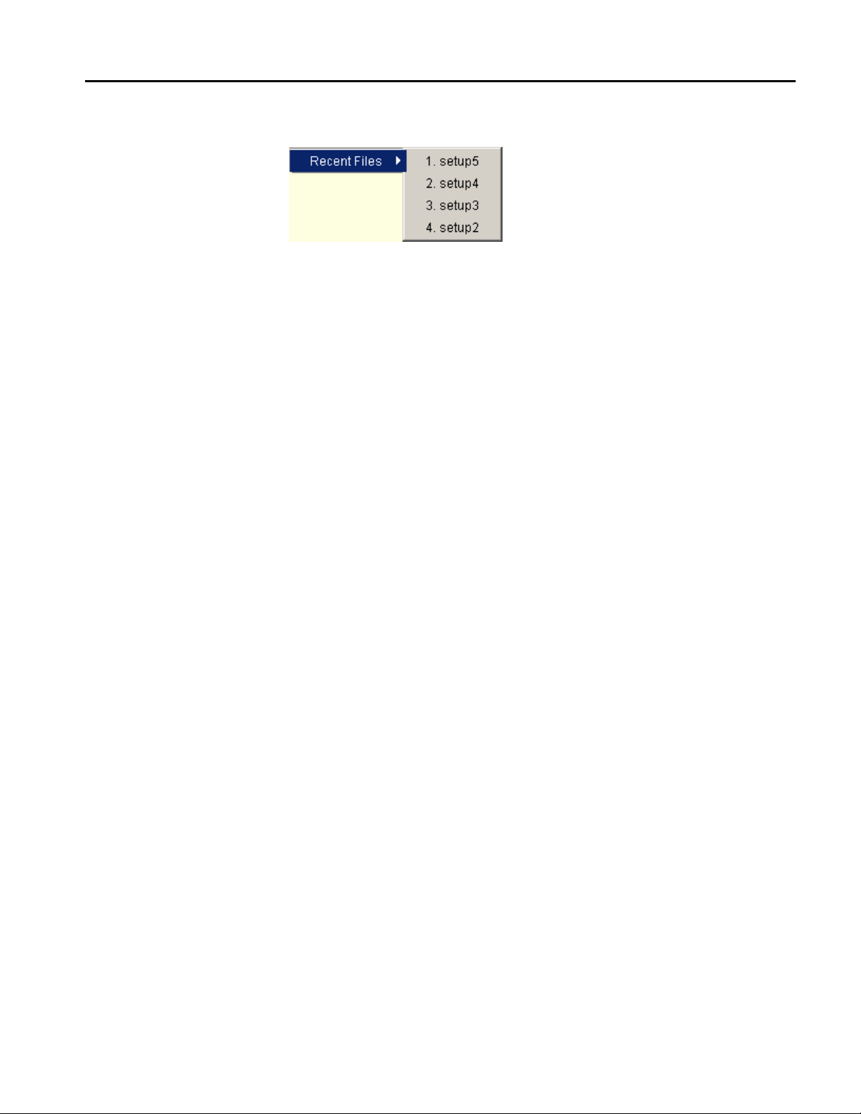
Operating Basic

Recall Recent Files Example

Figure 54: Recall Recent files example

Recalling a Setup File from a Prior Version of Software

Setup files that were saved using a prior version of the TDSJIT3 application may be recalled. For those features that were not present in the prior version, reasonable default settings are used. You may wish to verify that settings not specified by the old file are acceptable.

Note: Setup files from previous versions may include directory paths such as "C:\TekApplications\TDSJIT3\...", whereas the v2 application defaults to "C:\TekApplications\TDSJIT3v2\...". If you would like your converted setup files to use the TDSJITv2 directory, recall the existing setup file, use the Graphical User Interface to change any file paths to use the new directory structure, and then save the setup.

After you recall the setup file, you may save the setup again to create a setup file with the latest format. Use a different filename if you wish to retain the old setup file.

Vertical reference levels receive special attention during setup file conversion. If all of the reference levels for an active source are the default values (where High is set to 1.0 V, Mid is set to 0.0 V, Low is set to -1.0 V, and the Hysteresis is set to 0.03 V), then that source shall be configured for Automatic reference levels. Otherwise, the source shall be configured for Manual reference level and the reference levels in the setup shall be used exactly as they are. For more information, see the Automatic Versus Manual Reference Voltage Levels topic.

Some prior versions of the TDSJIT3 application used a configuration file ("jit3option.ini") to establish the order of the phase-locked loop used for clock recovery in PLL TIE measurements. The current TDSJIT3 application includes these controls and ignores the loop-order settings in the older configuration file. You can set these values manually, if necessary, and save a new setup file. After this, you can use the new setup file to ensure that the PLL settings are properly set.

Note: Setup files from the TDSJIT2 application are not supported.

TDSJIT3 v2 Jitter Analysis Online Help

Operating Basics

Docking and Undocking the Jitter Analysis Window

The Dock function positions and locks the TDSJIT3 v2 application in the lower half of the oscilloscope display and the oscilloscope application in the upper half of the display.

The Undock function unlocks the window and allows you to move the application to another position in the oscilloscope display or drag it to a second monitor; the oscilloscope display returns to full size.

The Dock and Undock functions are available under the File menus in the menu bar.

Acquisition Timeout Utility

The Acq Timeout utility sets the delay (in seconds) that the application allows between an acquisition start and when a waveform is expected.

• Auto allows the application to adjust the delay according to the record length

and measurement complexity

• User allows you to set the appropriate delay value from 30 seconds to 24

hours (86400 seconds) in 30 second increments

Warnings Utility

Figure 55: Acquisition Timeout options

The Warnings utility lists errors that have occurred and a brief description of each. To clear the contents from the file, select the Clear button.

Warnings are also designated with a yellow icon in the status bar along the bottom of the TDSJIT3 v2 application window. Once a message appears in the status bar, you can dismiss it by selecting the View Log button in the status bar, or by selecting the Clear results button. Neither action removes the message from the warnings log file.

icon and errors with a red

TDSJIT3 v2 Jitter Analysis Online Help

Tutorial

The purpose of this tutorial is to familiarize you with the basic functions of the TDSJIT3 v2 application and menus. This tutorial teaches you how to do the following basic tasks:

• Set up the application

• Take two types of measurements

• View the results as statistics and as plots

Before you begin the tutorial, you must do the following tasks:

• Set up the oscilloscope

• Start the application

• Recall the tutorial waveform

Note: The screen captures shown are from a TDS7000 oscilloscope; there may be minor differences in the screens from other oscilloscope models.

Setting Up the Oscilloscope

Starting the Application

Waveform Files

Recalling a Waveform File

To set up the oscilloscope, follow these steps:

1. In the oscilloscope menu bar, select File> Recall Default Setup to set the

oscilloscope to the default factory settings.

2. Press the individual CH1, CH2, CH3, and CH4 buttons as needed to remove

active waveforms from the display.

If you are using the TDSJIT3 v2 Essentials application, select Jitter Analysis Essentials.

If the Jitter Wizard displays, select the Cancel button.

The application includes two waveform files to use with this tutorial:

• j3clk1.wfm (clock signal)

• j3dat1.wfm (data signal)

The way you recall a waveform to reference memory depends on the oscilloscope model.

To recall a waveform file on most oscilloscopes, follow these steps:

1. In the oscilloscope menu bar, select File> Reference Waveforms> Reference

Setup. If the oscilloscope is in the Button mode, select the Ref button.

TDSJIT3 v2 Jitter Analysis Online Help 79

Tutorial

Ref1 is the default memory location to recall a waveform file. View the Oscilloscope Reference Memory Setup menu.

2. Select the

3. Navigate to the C:\TekApplications\TDSJIT3v2\Examples\waveforms

directory.

4. Select the j3clk1.wfm file, and then the

The oscilloscope recalls the waveform file to reference memory and displays the waveform when the recall is complete.

5. The way you return to the application depends on the oscilloscope model. To

return to the application, in the oscilloscope menu bar, select App> Restore

Application or select the application.

To recall a waveform file on TDS5000B oscilloscopes, follow these steps:

1. Select File> Recall. The Recall dialog appears.

2. In the left side of the dialog, select the Waveform icon.

3. Select Ref1, Ref2, Ref3, or Ref4 as the Destination option.

4. Browse to select the waveform to recall.

5. Select the Recall button. The oscilloscope recalls and activates the Reference

Waveform control window.

6. Select On to display the waveform.

7. Return to the application.

button for Recall Ref1 from File.

button.

button. View how to return to the

Note: The screen capture is from a TDS7000 oscilloscope. There are differences in the menu on other oscilloscope models.

Figure 56: Oscilloscope Reference Memory options

TDSJIT3 v2 Jitter Analysis Online Help

Tektronix TDSJIT3 v2 User manual

Specifications and Main Features

Frequently Asked Questions

User Manual

Table of Contents

List of Figures

List of Tables

General Safety Summary

Preface

5-Time Free Trial

Related Documentation

GPIB Information

Relevant Web Sites

Application CD Contents

Conventions

Types of Online Help Information

Using Online Help

Find Tab and Searches

Contacting Tektronix

Feedback

Getting Started

Differences between TDSJIT3 v2 Advanced and TDSJIT3 v2 Essentials

Compatibility

Requirements and Restrictions

Accessories

Installation

Operating Basics

General Information

Navigating the User Interface

Setting Up the Application for Analysis

Taking Measurements

Results as Statistics

Results as Plots

Working with Plots

Saving Information to Log Files

Saving and Recalling Setup Files

Tutorial

Setting Up the Oscilloscope