

Page 1

User Manual
TDSJIT1V2
Jitter Analysis Measurements Application
071-0875-00
This document supports software version 1.2.0
and above.
www.tektronix.com
Page 2

Copyright © T ektronix, Inc. All rights reserved. Licensed software products are owned by Tektronix or its suppliers and are
protected by United States copyright laws and international treaty provisions.
Use, duplication, or disclosure by the Government is subject to restrictions as set forth in subparagraph (c)(1)(ii) of the Rights
in T echnical Data and Computer Software clause at DFARS 252.227-7013, or subparagraphs (c)(1) and (2) of the
Commercial Computer Software – Restricted Rights clause at F AR 52.227-19, as applicable.
T ektronix products are covered by U.S. and foreign patents, issued and pending. Information in this publication supercedes
that in all previously published material. Specifications and price change privileges reserved.
T ektronix, Inc., P.O. Box 500, Beaverton, OR 97077
TEKTRONIX and TEK are registered trademarks of T ektronix, Inc.
Page 3

WARRANTY
T ektronix warrants that the media on which this software product is furnished and the encoding of the programs on the media
will be free from defects in materials and workmanship for a period of three (3) months from the date of shipment. If a
medium or encoding proves defective during the warranty period, T ektronix will provide a replacement in exchange for the
defective medium. Except as to the media on which this software product is furnished, this software product is provided “as
is” without warranty of any kind, either express or implied. T ektronix does not warrant that the functions contained in this
software product will meet Customer’s requirements or that the operation of the programs will be uninterrupted or error-free.
In order to obtain service under this warranty, Customer must notify Tektronix of the defect before the expiration of the
warranty period. If T ektronix is unable to provide a replacement that is free from defects in materials and workmanship
within a reasonable time thereafter, Customer may terminate the license for this software product and return this software
product and any associated materials for credit or refund.
THIS WARRANTY IS GIVEN BY TEKTRONIX IN LIEU OF ANY OTHER WARRANTIES, EXPRESS OR
IMPLIED. TEKTRONIX AND ITS VENDORS DISCLAIM ANY IMPLIED WARRANTIES OF
MERCHANTABILITY OR FITNESS FOR A PARTICULAR PURPOSE. TEKTRONIX’ RESPONSIBILITY TO
REPLACE DEFECTIVE MEDIA OR REFUND CUSTOMER’S PAYMENT IS THE SOLE AND EXCLUSIVE
REMEDY PROVIDED TO THE CUSTOMER FOR BREACH OF THIS WARRANTY. TEKTRONIX AND ITS
VENDORS WILL NOT BE LIABLE FOR ANY INDIRECT , SPECIAL, INCIDENTAL, OR CONSEQUENTIAL
DAMAGES IRRESPECTIVE OF WHETHER TEKTRONIX OR THE VENDOR HAS ADVANCE NOTICE OF
THE POSSIBILITY OF SUCH DAMAGES.
Page 4

Table of Contents
Getting Started
Operating Basics
General Safety Summary ix. . . . . . . . . . . . . . . . . . . . . . . . . . . . . . . . . . . . . . . . . .
Preface xi. . . . . . . . . . . . . . . . . . . . . . . . . . . . . . . . . . . . . . . . . . . . . . . . . . . . . . . . .
Related Documentation xi. . . . . . . . . . . . . . . . . . . . . . . . . . . . . . . . . . . . . . . . . . . .
Conventions xii. . . . . . . . . . . . . . . . . . . . . . . . . . . . . . . . . . . . . . . . . . . . . . . . . . . . .
Contacting T ektronix xii. . . . . . . . . . . . . . . . . . . . . . . . . . . . . . . . . . . . . . . . . . . . . .
Product Description 1–1. . . . . . . . . . . . . . . . . . . . . . . . . . . . . . . . . . . . . . . . .
Compatibility 1–1. . . . . . . . . . . . . . . . . . . . . . . . . . . . . . . . . . . . . . . . . . . . . . . . . . . .
Requirements and Restrictions 1–2. . . . . . . . . . . . . . . . . . . . . . . . . . . . . . . . . . . . . . .
Updates Through the Web Site 1–2. . . . . . . . . . . . . . . . . . . . . . . . . . . . . . . . . . . . . .
Accessories 1–2. . . . . . . . . . . . . . . . . . . . . . . . . . . . . . . . . . . . . . . . . . . . . . . . . . . . . .
Installation 1–3. . . . . . . . . . . . . . . . . . . . . . . . . . . . . . . . . . . . . . . . . . . . . . . .
Installing the Application 1–3. . . . . . . . . . . . . . . . . . . . . . . . . . . . . . . . . . . . . . . . . . .
Deskewing the Probes and Channels 1–4. . . . . . . . . . . . . . . . . . . . . . . . . . . . . . . . . .
Connecting to a System Under T est 1–9. . . . . . . . . . . . . . . . . . . . . . . . . . . . . . . . . . .
Basic Operations 2–1. . . . . . . . . . . . . . . . . . . . . . . . . . . . . . . . . . . . . . . . . . .
Application Menu Structure 2–1. . . . . . . . . . . . . . . . . . . . . . . . . . . . . . . . . . . . . . . . .
Main and Side Menus 2–1. . . . . . . . . . . . . . . . . . . . . . . . . . . . . . . . . . . . . . . . . .
Common Menu Items 2–2. . . . . . . . . . . . . . . . . . . . . . . . . . . . . . . . . . . . . . . . . .
Utility Menus 2–2. . . . . . . . . . . . . . . . . . . . . . . . . . . . . . . . . . . . . . . . . . . . . . . .
Using Basic Oscilloscope Functions 2–2. . . . . . . . . . . . . . . . . . . . . . . . . . . . . . . . . .
Using Local Help 2–2. . . . . . . . . . . . . . . . . . . . . . . . . . . . . . . . . . . . . . . . . . . . .
Returning to the Application 2–2. . . . . . . . . . . . . . . . . . . . . . . . . . . . . . . . . . . . .
Configuring the Display 2–4. . . . . . . . . . . . . . . . . . . . . . . . . . . . . . . . . . . . . . . . . . . .
Setting Up the Application 2–4. . . . . . . . . . . . . . . . . . . . . . . . . . . . . . . . . . . . . . . . . .
Selecting Measurements 2–4. . . . . . . . . . . . . . . . . . . . . . . . . . . . . . . . . . . . . . . .
Selecting a Measurement to Configure 2–6. . . . . . . . . . . . . . . . . . . . . . . . . . . . .
Configuring a Measurement 2–6. . . . . . . . . . . . . . . . . . . . . . . . . . . . . . . . . . . . .
Specifying Inputs 2–7. . . . . . . . . . . . . . . . . . . . . . . . . . . . . . . . . . . . . . . . . . . . .
Specifying Qualifiers 2–10. . . . . . . . . . . . . . . . . . . . . . . . . . . . . . . . . . . . . . . . . .
Specifying Gating 2–11. . . . . . . . . . . . . . . . . . . . . . . . . . . . . . . . . . . . . . . . . . . . .
Using Horizontal Check 2–11. . . . . . . . . . . . . . . . . . . . . . . . . . . . . . . . . . . . . . . .
Using Acquisition Timeout 2–11. . . . . . . . . . . . . . . . . . . . . . . . . . . . . . . . . . . . . .
T aking Measurements 2–12. . . . . . . . . . . . . . . . . . . . . . . . . . . . . . . . . . . . . . . . . . . . .
Acquiring Data 2–12. . . . . . . . . . . . . . . . . . . . . . . . . . . . . . . . . . . . . . . . . . . . . . .
Localizing Measurements 2–13. . . . . . . . . . . . . . . . . . . . . . . . . . . . . . . . . . . . . . .
W arning Messages 2–14. . . . . . . . . . . . . . . . . . . . . . . . . . . . . . . . . . . . . . . . . . . . . . . .
Analyzing the Results 2–14. . . . . . . . . . . . . . . . . . . . . . . . . . . . . . . . . . . . . . . . . . . . .
Viewing Statistics 2–15. . . . . . . . . . . . . . . . . . . . . . . . . . . . . . . . . . . . . . . . . . . . .
Viewing Plots 2–16. . . . . . . . . . . . . . . . . . . . . . . . . . . . . . . . . . . . . . . . . . . . . . . .
Clearing Results 2–20. . . . . . . . . . . . . . . . . . . . . . . . . . . . . . . . . . . . . . . . . . . . . .
Saving the Results to a File 2–20. . . . . . . . . . . . . . . . . . . . . . . . . . . . . . . . . . . . . . . . .
Logging Statistics 2–20. . . . . . . . . . . . . . . . . . . . . . . . . . . . . . . . . . . . . . . . . . . . .
Data Log File Format 2–21. . . . . . . . . . . . . . . . . . . . . . . . . . . . . . . . . . . . . . . . . .
TDSJIT1V2 Jitter Analysis Application User Manual
i
Page 5

Table of Contents
Logging Min/Max Waveforms 2–22. . . . . . . . . . . . . . . . . . . . . . . . . . . . . . . . . . .
Importing a Data Log File to a Personal Computer 2–23. . . . . . . . . . . . . . . . . . . . . . .
Saving and Recalling Setups 2–24. . . . . . . . . . . . . . . . . . . . . . . . . . . . . . . . . . . . . . . .
Saving a Setup 2–24. . . . . . . . . . . . . . . . . . . . . . . . . . . . . . . . . . . . . . . . . . . . . . . .
Recalling a Setup 2–25. . . . . . . . . . . . . . . . . . . . . . . . . . . . . . . . . . . . . . . . . . . . .
Exiting the Application 2–25. . . . . . . . . . . . . . . . . . . . . . . . . . . . . . . . . . . . . . . . . . . .
Tutorial 2–27. . . . . . . . . . . . . . . . . . . . . . . . . . . . . . . . . . . . . . . . . . . . . . . . . . .
Setting Up the Oscilloscope 2–27. . . . . . . . . . . . . . . . . . . . . . . . . . . . . . . . . . . . . . . . .
Starting the Application 2–27. . . . . . . . . . . . . . . . . . . . . . . . . . . . . . . . . . . . . . . . . . . .
Recalling a Waveform File 2–29. . . . . . . . . . . . . . . . . . . . . . . . . . . . . . . . . . . . . . . . . .
T aking a Clock Period Measurement 2–30. . . . . . . . . . . . . . . . . . . . . . . . . . . . . . . . . .
T aking a Clock Out Time Measurement 2–36. . . . . . . . . . . . . . . . . . . . . . . . . . . . . . .
Saving the Results to a Data Log File 2–40. . . . . . . . . . . . . . . . . . . . . . . . . . . . . . . . .
Viewing the RESULTS.CSV File (Data Log) 2–43. . . . . . . . . . . . . . . . . . . . . . . . . . .
Stopping the Tutorial 2–43. . . . . . . . . . . . . . . . . . . . . . . . . . . . . . . . . . . . . . . . . . . . . .
Returning to the Tutorial 2–43. . . . . . . . . . . . . . . . . . . . . . . . . . . . . . . . . . . . . . . . . . .
GPIB Program Example 2–45. . . . . . . . . . . . . . . . . . . . . . . . . . . . . . . . . . . . .
Guidelines 2–45. . . . . . . . . . . . . . . . . . . . . . . . . . . . . . . . . . . . . . . . . . . . . . . . . . . . . .
Program Example 2–45. . . . . . . . . . . . . . . . . . . . . . . . . . . . . . . . . . . . . . . . . . . . . . . . .
Reference
Appendices
Menu Structure 3–1. . . . . . . . . . . . . . . . . . . . . . . . . . . . . . . . . . . . . . . . . . . .
Parameters 3–3. . . . . . . . . . . . . . . . . . . . . . . . . . . . . . . . . . . . . . . . . . . . . . . .
Measurements Menus 3–3. . . . . . . . . . . . . . . . . . . . . . . . . . . . . . . . . . . . . . . . . . . . . .
Select Measurements Menu 3–3. . . . . . . . . . . . . . . . . . . . . . . . . . . . . . . . . . . . .
Configure Selected Menu 3–3. . . . . . . . . . . . . . . . . . . . . . . . . . . . . . . . . . . . . . .
Inputs Menus 3–4. . . . . . . . . . . . . . . . . . . . . . . . . . . . . . . . . . . . . . . . . . . . . . . . . . . .
Main Input and 2nd Input Menus 3–4. . . . . . . . . . . . . . . . . . . . . . . . . . . . . . . . .
Qualifier Input Menu 3–6. . . . . . . . . . . . . . . . . . . . . . . . . . . . . . . . . . . . . . . . . .
Acquisition Timeout Menu 3–6. . . . . . . . . . . . . . . . . . . . . . . . . . . . . . . . . . . . . .
Results Menus 3–6. . . . . . . . . . . . . . . . . . . . . . . . . . . . . . . . . . . . . . . . . . . . . . . . . . .
Plot Menus 3–6. . . . . . . . . . . . . . . . . . . . . . . . . . . . . . . . . . . . . . . . . . . . . . . . . . . . . .
Histogram Plot Menu 3–7. . . . . . . . . . . . . . . . . . . . . . . . . . . . . . . . . . . . . . . . . .
Cycle Trend Menu 3–7. . . . . . . . . . . . . . . . . . . . . . . . . . . . . . . . . . . . . . . . . . . .
Time T rend Menu 3–8. . . . . . . . . . . . . . . . . . . . . . . . . . . . . . . . . . . . . . . . . . . . .
Spectrum Menu 3–8. . . . . . . . . . . . . . . . . . . . . . . . . . . . . . . . . . . . . . . . . . . . . . .
Log Menus 3–9. . . . . . . . . . . . . . . . . . . . . . . . . . . . . . . . . . . . . . . . . . . . . . . . . . . . . .
Results Menu 3–9. . . . . . . . . . . . . . . . . . . . . . . . . . . . . . . . . . . . . . . . . . . . . . . .
Min/Max Wfms Menu 3–9. . . . . . . . . . . . . . . . . . . . . . . . . . . . . . . . . . . . . . . . .
Control Menu 3–9. . . . . . . . . . . . . . . . . . . . . . . . . . . . . . . . . . . . . . . . . . . . . . . . . . . .
Utility Menus 3–10. . . . . . . . . . . . . . . . . . . . . . . . . . . . . . . . . . . . . . . . . . . . . . . . . . . .
Appendix A: Measurement Algorithms A–1. . . . . . . . . . . . . . . . . . . . . . . .
Oscilloscope Setup Guidelines A–1. . . . . . . . . . . . . . . . . . . . . . . . . . . . . . . . . . . . . . .
T est Methodology A–1. . . . . . . . . . . . . . . . . . . . . . . . . . . . . . . . . . . . . . . . . . . . . . . . .
Edge-Timing Measurements A–2. . . . . . . . . . . . . . . . . . . . . . . . . . . . . . . . . . . . . . . .
Single Waveform Measurements A–2. . . . . . . . . . . . . . . . . . . . . . . . . . . . . . . . . . . . .
Rise Time Measurement A–2. . . . . . . . . . . . . . . . . . . . . . . . . . . . . . . . . . . . . . . .
Fall Time Measurement A–3. . . . . . . . . . . . . . . . . . . . . . . . . . . . . . . . . . . . . . . .
ii
TDSJIT1V2 Jitter Analysis Application User Manual
Page 6

Table of Contents
Positive and Negative Width Measurements A–3. . . . . . . . . . . . . . . . . . . . . . . .
High Time Measurement A–3. . . . . . . . . . . . . . . . . . . . . . . . . . . . . . . . . . . . . . .
Low Time Measurement A–4. . . . . . . . . . . . . . . . . . . . . . . . . . . . . . . . . . . . . . . .
Clock Frequency Measurement A–4. . . . . . . . . . . . . . . . . . . . . . . . . . . . . . . . . .
Clock Period Measurement A–4. . . . . . . . . . . . . . . . . . . . . . . . . . . . . . . . . . . . . .
Cycle-Cycle Period Measurement A–4. . . . . . . . . . . . . . . . . . . . . . . . . . . . . . . .
N-Cycle Period Measurement A–5. . . . . . . . . . . . . . . . . . . . . . . . . . . . . . . . . . . .
Positive and Negative Cycle-to-Cycle Duty Measurements A–5. . . . . . . . . . . . .
Positive and Negative Duty Cycle Measurements A–5. . . . . . . . . . . . . . . . . . . .
Clock TIE Measurement A–6. . . . . . . . . . . . . . . . . . . . . . . . . . . . . . . . . . . . . . . .
Data Frequency Measurement A–6. . . . . . . . . . . . . . . . . . . . . . . . . . . . . . . . . . .
Data Period Measurement A–6. . . . . . . . . . . . . . . . . . . . . . . . . . . . . . . . . . . . . . .
Data TIE Measurement A–7. . . . . . . . . . . . . . . . . . . . . . . . . . . . . . . . . . . . . . . . .
Dual Waveform Measurements A–7. . . . . . . . . . . . . . . . . . . . . . . . . . . . . . . . . . . . . .
Setup Time Measurement A–7. . . . . . . . . . . . . . . . . . . . . . . . . . . . . . . . . . . . . . .
Hold Time Measurement A–7. . . . . . . . . . . . . . . . . . . . . . . . . . . . . . . . . . . . . . .
Clock Out Time Measurement A–8. . . . . . . . . . . . . . . . . . . . . . . . . . . . . . . . . . .
Skew Measurement A–8. . . . . . . . . . . . . . . . . . . . . . . . . . . . . . . . . . . . . . . . . . . .
Appendix B: GPIB Command Syntax B–1. . . . . . . . . . . . . . . . . . . . . . . . . .
Appendix C: Error Codes C–1. . . . . . . . . . . . . . . . . . . . . . . . . . . . . . . . . . . .
Appendix D: Example Program to Copy Large Files D–1. . . . . . . . . . . . .
Index
TDSJIT1V2 Jitter Analysis Application User Manual
iii
Page 7

Table of Contents
List of Figures
Figure 1–1: TDSJIT1V2 Jitter Analysis Application 1–1. . . . . . . . . . . . . .
Figure 1–2: Typical signal path skew 1–5. . . . . . . . . . . . . . . . . . . . . . . . . . .
Figure 1–3: Vertical Autoset complete 1–6. . . . . . . . . . . . . . . . . . . . . . . . . .
Figure 1–4: Accessing the Deskew utility 1–7. . . . . . . . . . . . . . . . . . . . . . .
Figure 1–5: The Deskew menu 1–7. . . . . . . . . . . . . . . . . . . . . . . . . . . . . . . .
Figure 1–6: Deskewing complete 1–8. . . . . . . . . . . . . . . . . . . . . . . . . . . . . .
Figure 1–7: Adjusted skew 1–9. . . . . . . . . . . . . . . . . . . . . . . . . . . . . . . . . . .
Figure 2–1: Returning to the application 2–3. . . . . . . . . . . . . . . . . . . . . . .
Figure 2–2: How to determine voltage reference levels 2–8. . . . . . . . . . . .
Figure 2–3: Example of the results and display formats 2–14. . . . . . . . . . .
Figure 2–4: A RESULTS.CSV file viewed in a spreadsheet
program 2–15. . . . . . . . . . . . . . . . . . . . . . . . . . . . . . . . . . . . . . . . . . . . . . .
Figure 2–5: Results Details menu, example of three measurements 2–16. .
Figure 2–6: Starting the application 2–28. . . . . . . . . . . . . . . . . . . . . . . . . . .
Figure 2–7: TDSJIT1V2 application initial display 2–28. . . . . . . . . . . . . . .
Figure 2–8: Recalling a waveform to a reference memory 2–29. . . . . . . . .
Figure 2–9: J1V2_CLK.WFM recalled to Ref1 2–30. . . . . . . . . . . . . . . . . .
Figure 2–10: Main Input menu setup 2–31. . . . . . . . . . . . . . . . . . . . . . . . . .
Figure 2–11: Clock Period lesson: Results Summary readout 2–32. . . . . .
Figure 2–12: Setup for a Histogram plot 2–32. . . . . . . . . . . . . . . . . . . . . . . .
Figure 2–13: Results as a Histogram plot 2–33. . . . . . . . . . . . . . . . . . . . . . .
Figure 2–14: Results as a Time Trend plot 2–34. . . . . . . . . . . . . . . . . . . . . .
Figure 2–15: Setup for a Spectrum plot 2–35. . . . . . . . . . . . . . . . . . . . . . . .
Figure 2–16: Results as a Spectrum plot 2–35. . . . . . . . . . . . . . . . . . . . . . . .
Figure 2–17: Results as a Cycle Trend plot 2–36. . . . . . . . . . . . . . . . . . . . . .
Figure 2–18: J1V2_CLK.WFM recalled to Ref3 2–37. . . . . . . . . . . . . . . . .
Figure 2–19: Selected Measurements list 2–38. . . . . . . . . . . . . . . . . . . . . . .
Figure 2–20: 2nd Input menu setup 2–39. . . . . . . . . . . . . . . . . . . . . . . . . . . .
Figure 2–21: Clock Out Time lesson: Results Summary results 2–39. . . . .
Figure 2–22: Result Details shows the statistical values for all
measurements 2–40. . . . . . . . . . . . . . . . . . . . . . . . . . . . . . . . . . . . . . . . . .
Figure 2–23: Log Results menu 2–41. . . . . . . . . . . . . . . . . . . . . . . . . . . . . . .
Figure 2–24: Path to the RESULTS.CSV file on the hard drive 2–42. . . . .
Figure 2–25: Copying the RESULTS.CSV file to a floppy disk 2–42. . . . .
Figure 3–1: Menu structure 3–1. . . . . . . . . . . . . . . . . . . . . . . . . . . . . . . . . .
iv
TDSJIT1V2 Jitter Analysis Application User Manual
Page 8

List of Tables
Table of Contents
Table 1–1: Default waveform assignments 1–10. . . . . . . . . . . . . . . . . . . . . .
Table 2–1: Common menu items 2–2. . . . . . . . . . . . . . . . . . . . . . . . . . . . . .
Table 2–2: Utility menus 2–2. . . . . . . . . . . . . . . . . . . . . . . . . . . . . . . . . . . .
Table 2–3: Default directory names 2–3. . . . . . . . . . . . . . . . . . . . . . . . . . .
Table 2–4: File name extensions 2–3. . . . . . . . . . . . . . . . . . . . . . . . . . . . . .
Table 2–5: Display Options menu selections 2–4. . . . . . . . . . . . . . . . . . . .
Table 2–6: Select Measurement menu selections 2–5. . . . . . . . . . . . . . . . .
Table 2–7: Measurements and configuration selections 2–6. . . . . . . . . . .
Table 2–8: Main Input and 2nd Input menus selections 2–8. . . . . . . . . . .
Table 2–9: Autoset Ref Levels menu selections 2–9. . . . . . . . . . . . . . . . . .
Table 2–10: Deskew menu selections 2–10. . . . . . . . . . . . . . . . . . . . . . . . . .
Table 2–11: Qualifier Input menu selections 2–10. . . . . . . . . . . . . . . . . . . .
Table 2–12: Acquisition Timeout menu selections 2–12. . . . . . . . . . . . . . . .
Table 2–13: Control menu selections 2–13. . . . . . . . . . . . . . . . . . . . . . . . . .
Table 2–14: Plot Type selections 2–17. . . . . . . . . . . . . . . . . . . . . . . . . . . . . .
Table 2–15: Vert/Horiz Axis Histogram menu selections 2–18. . . . . . . . . .
Table 2–16: Vert/Horiz Axis Time Trend menu selection 2–19. . . . . . . . . .
Table 2–17: Spectrum menu selection 2–19. . . . . . . . . . . . . . . . . . . . . . . . . .
Table 2–18: Vert/Horiz Axis Cycle Trend menu selections 2–20. . . . . . . . .
Table 2–19: Log Results menu selections 2–21. . . . . . . . . . . . . . . . . . . . . . .
Table 2–20: Log Min/Max Wfms menu selections 2–22. . . . . . . . . . . . . . . .
Table 2–21: File names for Min/Max waveforms 2–22. . . . . . . . . . . . . . . .
Table 2–22: Tutorial waveforms and signal types 2–29. . . . . . . . . . . . . . . .
Table 3–1: Configure Selected menu parameters 3–4. . . . . . . . . . . . . . . .
Table 3–2: Main Input and 2nd Input menu parameters 3–5. . . . . . . . . .
Table 3–3: Autoset Ref Level menu parameters 3–5. . . . . . . . . . . . . . . . .
Table 3–4: Deskew menu parameters 3–5. . . . . . . . . . . . . . . . . . . . . . . . . .
Table 3–5: Qualifier Input menu parameters 3–6. . . . . . . . . . . . . . . . . . .
Table 3–6: Acquisition Timeout menu parameters 3–6. . . . . . . . . . . . . . .
Table 3–7: Histogram Plot menu parameters 3–7. . . . . . . . . . . . . . . . . . .
Table 3–8: Horizontal Center and Span parameters by
measurement 3–7. . . . . . . . . . . . . . . . . . . . . . . . . . . . . . . . . . . . . . . . . . .
Table 3–9: Cycle Trend Plot menu parameters 3–7. . . . . . . . . . . . . . . . . .
Table 3–10: Time Trend Plot menu parameters 3–8. . . . . . . . . . . . . . . . .
TDSJIT1V2 Jitter Analysis Application User Manual
v
Page 9

Table of Contents
Table 3–11: Spectrum Plot menu parameters 3–8. . . . . . . . . . . . . . . . . . .
Table 3–12: Log Results menu parameters 3–9. . . . . . . . . . . . . . . . . . . . .
Table 3–13: Log Min/Max Wfms menu parameters 3–9. . . . . . . . . . . . . .
Table 3–14: Control menu parameters 3–9. . . . . . . . . . . . . . . . . . . . . . . . .
Table 3–15: Utility menus and parameters 3–10. . . . . . . . . . . . . . . . . . . . .
Table B–1: VARIABLE:VALUE TDS COMMAND arguments and
queries B–2. . . . . . . . . . . . . . . . . . . . . . . . . . . . . . . . . . . . . . . . . . . . . . . .
Table B–2: Measurement results queries B–3. . . . . . . . . . . . . . . . . . . . . . .
Table C–1: Error codes, descriptions and solutions C–1. . . . . . . . . . . . . .
vi
TDSJIT1V2 Jitter Analysis Application User Manual
Page 10

General Safety Summary
Review the following safety precautions to avoid injury and prevent damage to
this product or any products connected to it. To avoid potential hazards, use this
product only as specified.
Only qualified personnel should perform service procedures.
While using this product, you may need to access other parts of the system. Read
the General Safety Summary in other system manuals for warnings and cautions
related to operating the system.
To Avoid Fire or Personal Injury
Symbols and Terms
Connect and Disconnect Properly . Do not connect or disconnect probes or test
leads while they are connected to a voltage source.
Observe All Terminal Ratings. To avoid fire or shock hazard, observe all ratings
and markings on the product. Consult the product manual for further ratings
information before making connections to the product.
Do Not Operate With Suspected Failures. If you suspect there is damage to this
product, have it inspected by qualified service personnel.
T erms in this Manual. These terms may appear in this manual:
WARNING. Warning statements identify conditions or practices that could result
in injury or loss of life.
CAUTION. Caution statements identify conditions or practices that could result in
damage to this product or other property.
T erms on the Product. These terms may appear on the product:
DANGER indicates an injury hazard immediately accessible as you read the
marking.
WARNING indicates an injury hazard not immediately accessible as you read the
marking.
CAUTION indicates a hazard to property including the product.
Symbols on the Product. The following symbol may appear on the product:
CAUTION Refer to Manual
TDSJIT1V2 Jitter Analysis Application User Manual
vii
Page 11

General Safety Summary
viii
TDSJIT1V2 Jitter Analysis Application User Manual
Page 12

Preface
This manual contains operating information for the TDSJIT1V2 Jitter Analysis
Application. The manual consists of the following chapters:
H The Getting Started chapter briefly describes the TDSJIT1V2 Jitter Analysis
Application, lists oscilloscope compatibility, and provides installation
instructions.
H The Operating Basics chapter covers basic operating principles of the
application and includes a tutorial that teaches you how to set up the
application to acquire a waveform, take measurements, and view the results.
To show you how to operate the application using GPIB commands, this
chapter includes a simple GPIB program.
H The Reference chapter includes a diagram of the menu structure and
descriptions of parameters.
H The Measurement Algorithms appendix contains information on measure-
ment guidelines and on how the application takes the measurements.
H The GPIB Command Syntax appendix contains a list of arguments and values
that you can use with the GPIB commands and their associated parameters.
Related Documentation
H The Error Codes appendix contains a list of error codes, descriptions of the
errors, and possible solutions to correct the problem.
H The Example Program to Copy Large Files appendix contains an example of
a GPIB program you can use to transfer large files to a personal computer.
The user manual for your oscilloscope provides general information on how to
operate the oscilloscope.
Programmer information in the online help for your oscilloscope provides details
on how to use GPIB commands to control the oscilloscope. You can also
download the tds6prog.zip file (online help) with examples from the Tektronix
web site. The file can be used for all supported oscilloscopes. Refer to Updates
Through the Web Site on page 1–2 for information on how to download the file.
TDSJIT1V2 Jitter Analysis Application User Manual
ix
Page 13

Preface
Conventions
Contacting Tektronix
This manual uses the following conventions:
H This manual refers to the TDSJIT1V2 Jitter Analysis Application as the
TDSJIT1V2 application or as the application.
H When steps require that you make a sequence of selections using front-panel
controls and menu buttons, an arrow ( ➞
) marks each transition between a
front-panel button and a menu, or between menus. Names that are for a main
menu or side menu item are clearly indicated: Press VERTICAL MENU ➞
Coupling (main) ➞ DC (side) ➞ Bandwidth (main) ➞ 250 MHz (side).
Phone 1-800-833-9200*
Address Tektronix, Inc.
Department or name (if known)
14200 SW Karl Braun Drive
P.O. Box 500
Beaverton, OR 97077
USA
Web site www.tektronix.com
Sales support 1-800-833-9200, select option 1*
Service support 1-800-833-9200, select option 2*
Technical support Email: techsupport@tektronix.com
1-800-833-9200, select option 3*
1-503-627-2400
6:00 a.m. – 5:00 p.m. Pacific time
* This phone number is toll free in North America. After office hours, please leave a
voice mail message.
Outside North America, contact a Tektronix sales office or distributor; see the
Tektronix web site for a list of offices.
x
TDSJIT1V2 Jitter Analysis Application User Manual
Page 14

Getting Started
Page 15

Product Description
The TDSJIT1V2 Jitter Analysis Application is a Java-based application that
enhances basic capabilities of some Tektronix oscilloscopes.
The application provides jitter analysis measurements, can display the statistical
results of up to six measurements, can display the results as plots, can save the
results to a data log file, and can save the worst case waveforms to files.
Figure 1–1 shows an example of a Clock Period measurement displayed as a
Histogram plot.
694C
Figure 1–1: TDSJIT1V2 Jitter Analysis Application
Compatibility
The Jitter Analysis Application V 1.2.0 and above is compatible with the
TDS694C oscilloscope with firmware version 6.2 and above, and with TDS784D
and TDS794D oscilloscopes with firmware version 6.6e and above, or 7.2e and
above depending on the acquisition board in the oscilloscope.
For information on how to get the current firmware, contact your local Tektronix
distributor or sales office.
For a current list of compatible oscilloscopes, see the Software and Drivers
category in the Tektronix, Inc. web site (www.tektronix.com).
TDSJIT1V2 Jitter Analysis Application User Manual
1–1
Page 16

Product Description
Requirements and Restrictions
The TDS Run-Time Environment V1.2.0 or above must be installed on the
oscilloscope to operate the TDSJIT1V2 application and use GPIB commands.
Updates Through the Web Site
You can find information about this and other applications at the Tektronix, Inc.
web site. Check this site for application updates and for other free applications.
To install an application update, you will need to download it from the web site
to a hard disk, copy it to a blank DOS-formatted floppy disk, and then install it
on your oscilloscope.
NOTE. More information about changes to the application or installation is in a
Readme.txt file on the web site. You should read it before you continue.
Accessories
To copy an application from the web site, follow these steps:
1. Access www .tekrronix.com/Measurement/Support/Scopes.
2. Scroll through the files to the application that you want, select the file, and
download it to your hard disk drive. If necessary, unzip the file.
NOTE. To ensure that the files were downloaded successfully, always unzip the
files on a hard disk before copying them to a floppy disk.
3. Copy the application from the hard disk to a blank, DOS-formatted floppy
disk. Only copy one application on to one floppy disk.
4. Follow the Installing the Application procedure on page 1–3.
There are no standard accessories for this product other than this manual.
1–2
TDSJIT1V2 Jitter Analysis Application User Manual
Page 17

Installation
This section contains information on the following tasks:
H Installing the application
H Deskewing probes and channels
H Connecting to a system under test
Installing the Application
The TDSJIT1V2 floppy disk contains the TDSJIT1V2 Jitter Analysis Application. You can download updates, if any, from the Tektronix ftp site through a
web browser.
NOTE. To operate the TDSJIT1V2 application, the TDS Run-Time Environment
V1.2.0 or above must be installed on the oscilloscope.
To install the application from the floppy disk to your oscilloscope, follow these
steps:
1. Power off the oscilloscope.
NOTE. Additional information about the application or installation is located in
a Readme.txt file on the floppy disk. You should insert the floppy disk into a
DOS-based personal computer and read the Readme.txt file before you continue.
If you are updating the application, the Readme.txt file on the Tektronix ftp site
supercedes the Readme.txt file on the TDSJIT1V2 floppy disk.
2. Insert the disk in the floppy disk drive, and power on the oscilloscope.
NOTE. To verify that the TDS Run-Time Environment V1.2.0 or above is
installed, watch for the abbreviated name, RTE, and version number to appear
at the top of the display when you power on the oscilloscope. If they do not
appear, contact your local Tektronix sales office.
After performing the power-on selftest, the oscilloscope automatically begins the
installation procedure.
TDSJIT1V2 Jitter Analysis Application User Manual
1–3
Page 18

Installation
As the application loads from the disk, the oscilloscope displays a clock icon to
indicate that it is busy. Also, the floppy disk drive LED is on, indicating activity.
If the clock icon continues to display after the floppy disk LED has gone out, a
problem has occurred with the installation. Repeat the above procedure. If the
problem persists, contact your Tektronix representative.
When the installation is complete, an Installation Complete message displays.
3. Remove the floppy disk, and cycle the power to the oscilloscope.
Deskewing the Probes and Channels
To ensure accurate results for two-channel measurements, it is important to first
deskew the probes and oscilloscope channels before you take measurements from
your system under test (SUT). Deskewing is where the oscilloscope adjusts the
relative delay between signals to accurately time correlate the displayed
waveforms.
NOTE. To produce good deskew results, you should connect the probes to the
fastest signal in your SUT.
The application includes an automated deskew utility that you can use to deskew
any pair of oscilloscope channels. The following procedure describes how to
deskew two channels. Channel 1 (and the probe connected to it) is the reference
point used to deskew channel 2. The steps to deskew the third and fourth
channels are the same.
WARNING. To avoid electric shock, you must ensure that power is removed from
the SUT before attaching probes to it. Do not touch exposed conductors except
with the properly rated probe tips. Refer to the probe manual for proper use.
To deskew a pair of probes and oscilloscope channels, follow these steps:
1. Connect similar probes to CH 1 and CH 2 on the oscilloscope.
2. Connect the probes to the fastest signal in your SUT.
3. To set up the oscilloscope, press the AUTOSET front-panel button.
Figure 1–2 shows an example of signal path skew found in similar probes.
1–4
TDSJIT1V2 Jitter Analysis Application User Manual
Page 19

Installation
Figure 1–2: T ypical signal path skew
4. Start the application as described on page 2–30.
5. Press Inputs (main) ➞ Main (side) ➞ Source (side) and select Ch1. The
waveform displayed as the source for the Main Input is the reference point to
which the remaining channels are deskewed.
6. Press Vertical Autoset (side). Figure 1–3 shows the results of a the Vertical
Austoset.
TDSJIT1V2 Jitter Analysis Application User Manual
1–5
Page 20

Installation
Figure 1–3: Vertical Autoset complete
7. Press OK (side).
8. Press Done (side).
9. Press 2nd (side) ➞ Source (side) and select Ch2. The waveform displayed as
the source for the 2nd Input is the channel to be deskewed.
10. Press Vertical Autoset (side) and then OK (side).
11. Press – more – 1 of 2 (side) ➞ Deskew ... (side). Figure 1–4 shows how to
access the Deskew menu. Figure 1–5 shows the Deskew menu.
1–6
TDSJIT1V2 Jitter Analysis Application User Manual
Page 21

Installation
Figure 1–4: Accessing the Deskew utility
Figure 1–5: The Deskew menu
TDSJIT1V2 Jitter Analysis Application User Manual
1–7
Page 22

Installation
12. Enter appropriate values for the Upper Range and the Lower Range side
menu items.
13. To start the deskew utility, press Perform Deskew (side).
Figure 1–6 shows an example of the utility when it is finished.
1–8
Figure 1–6: Deskewing complete
14. Press OK (side).
Figure 1–7 shows an example of using the oscilloscope V Bar cursors to
measure the adjusted skew. In this example, the skew between channels 1
and 2 was reduced to 320 ps.
TDSJIT1V2 Jitter Analysis Application User Manual
Page 23

Installation
Figure 1–7: Adjusted skew
15. Press the SHIFT, and then the APPLICATION front-panel menu button to
return to the application.
16. Do not change the Main Input Source channel, and deskew the remaining
channels if you will be using them to take jitter measurements.
Connecting to a System Under Test
Although you can use any compatible probes to connect between your SUT
(system under test) and oscilloscope, Tektronix P6330 3 GHz Differential probes
and P6249 4 GHz Differential probes are recommended. One connection is
usually to a clock signal.
The General, Clock, and Data measurements require one input waveform. The
Clock-Data and the Ch-Ch measurements require two input waveforms.
TDSJIT1V2 Jitter Analysis Application User Manual
1–9
Page 24

Installation
Table 1–1 shows the default channel-to-waveform and reference waveform-to
plot assignments. You can change the assignments to match your configuration.
T able 1–1: Default waveform assignments
Channel or reference Waveform assignment
Ch 1 Main input waveform, such as a clock signal
Ch 2 Second (2nd) input waveform
Ch 3 Qualifier input waveform
Ref1 Histogram plot format for the first measurement
Ref2 Time Trend plot format for the first measurement
Ref3 Cycle Trend plot format for the first measurement
Math1 Spectrum plot format for the first measurement
WARNING. To avoid electric shock, you must ensure that power is removed from
the SUT before attaching probes to it. Do not touch exposed conductors except
with the properly rated probe tips. Refer to the probe manual for proper use.
Power down the SUT before connecting the probes to it.
1–10
TDSJIT1V2 Jitter Analysis Application User Manual
Page 25

Operating Basics
Page 26

Basic Operations
This section contains information on the following topics and tasks:
H Application interface
H Using basic oscilloscope functions
H Setting up the application
H Taking measurements
H Warning messages
H Analyzing the results
H Saving the results to a file
H Importing a data log file
H Saving and recalling setups
H Exiting the application
Application Menu Structure
There are two types of menus in the application menu structure: main menus and
side menus. Some side menus contain common items as shown in Table 2–1.
Main and Side Menus
The main menu names appear in the bottom of the display, and the side menu
names appear on the right side of the display. To see the complete application
menu structure, refer to Figure 3–1 on page 3–1.
When you press the front-panel button associated with a main menu, the side
menu changes. In many cases, when you press a side menu, new side menu items
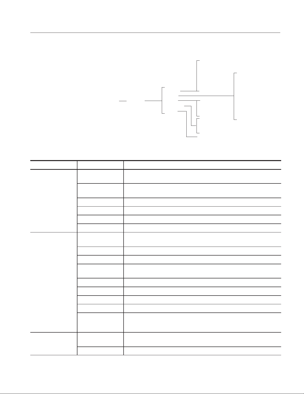
appear. As an example, the next figure shows you how to access the Help
selections through the main Utility menu and the Help side menu.
Main menu Side menu Side menu item
Utility
Help
First Page
Next Page
Previous Page
Last Page
Quit Help
TDSJIT1V2 Jitter Analysis Application User Manual
2–1
Page 27

Basic Operations
Common Menu Items
Utility Menus
Table 2–1 lists common side menu items.
T able 2–1: Common menu items
Menu item Description
Cancel Returns to the previous menu without performing the operation specific
to the current menu
Done Indicates that you are through making changes to that set of side menus;
the application returns to the previous menu
OK Confirms an action
–more–
x of y
Scrolls to another page of a menu where x is the current page and y is
the total number of pages
Table 2–2 lists the Utility menus.
T able 2–2: Utility menus
Utility name Description
Help Accesses the online help pages and displays useful information on the
application
Exit Exits the application
Display Options Accesses other menus where you can change display settings, such as
Save/Recall Setup Accesses the save and the recall menus for application setups
Using Basic Oscilloscope Functions
You can use the Utility menu to access help information about the application.
You can also use other oscilloscope functions and easily return to the application.
Using Local Help
Returning to the
Application
The application includes local help information about the measurements modes,
with some explanation of the individual controls.
To display the local help, follow these steps:
1. Press Utility (main) ➞ Help (side).
2. Use the side menu buttons to navigate through the help.
You can easily switch between the TDSJIT1V2 application and other oscilloscope functions.
whether the dialog box is opaque or transparent
2–2
TDSJIT1V2 Jitter Analysis Application User Manual
Page 28
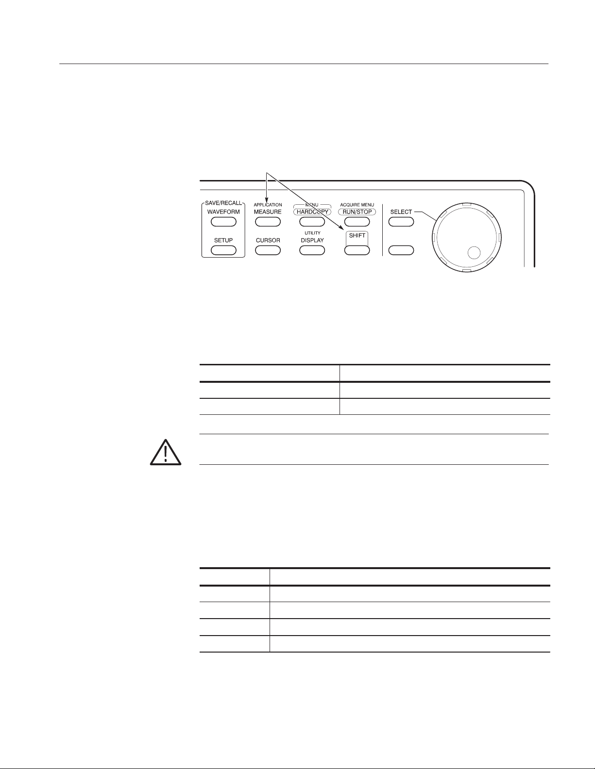
Basic Operations
To access other oscilloscope functions, press the desired front-panel control. To
return to the application, press the SHIFT and then the APPLICATION
front-panel menu buttons as shown in Figure 2–1.
Press the SHIFT and then the APPLICATION button to return to the application.
Figure 2–1: Returning to the application
Default Directories. Table 2–3 lists default directory names and their use.
T able 2–3: Default directory names
Directory name Used for
hd0:/APP/TDSJITV2/TEMP Setup files, data log files, and min/max waveform files
hd0:/WFMS Waveform files used in the tutorial
WARNING. To avoid corrupting the application, do not access the SYSTEM
directory. Some files are only for internal use by the application.
File Name Extensions. Table 2–4 lists file name extensions used or generated by
the application.
T able 2–4: File name extensions
Extension Type
.csv Log file that uses a “comma separated variable” format
.wfm Waveform file that can be recalled into a reference memory
.ini Application setup file
.set Oscilloscope setup file created by the application
TDSJIT1V2 Jitter Analysis Application User Manual
2–3
Page 29

Basic Operations
Configuring the Display
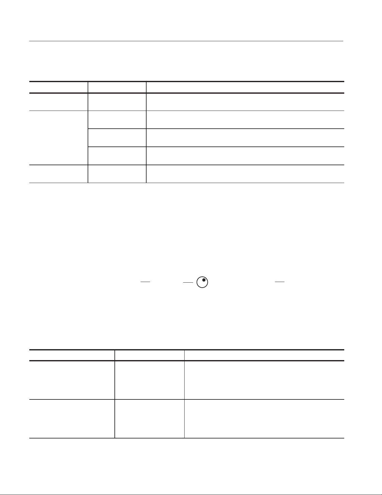
You can change how dialog boxes appear on your oscilloscope, as well as the
color of waveforms. The next figure shows how to access the Display Options
menu, and Table 2–5 lists the options with a brief description of each.
Main menu Side menu Side menu item
Utility Display Options
Dialog Box
Box Position
Box Style
Color Theme
Done
T able 2–5: Display Options menu selections
Selection Description
Dialog Box
Box Position Positions the dialog box in the display to the left, middle, or right
Makes dialog boxes visible or invisible
Box Style Selects the style of dialog boxes to be opaque or transparent
Color Theme Selects a set of colors for waveforms and dialog boxes; the application
Setting Up the Application
You can set up the application to take up to six measurements at the same time.
In addition, you can plot the results in four formats, and save the statistical
results or the worst case waveforms to a file to view later.
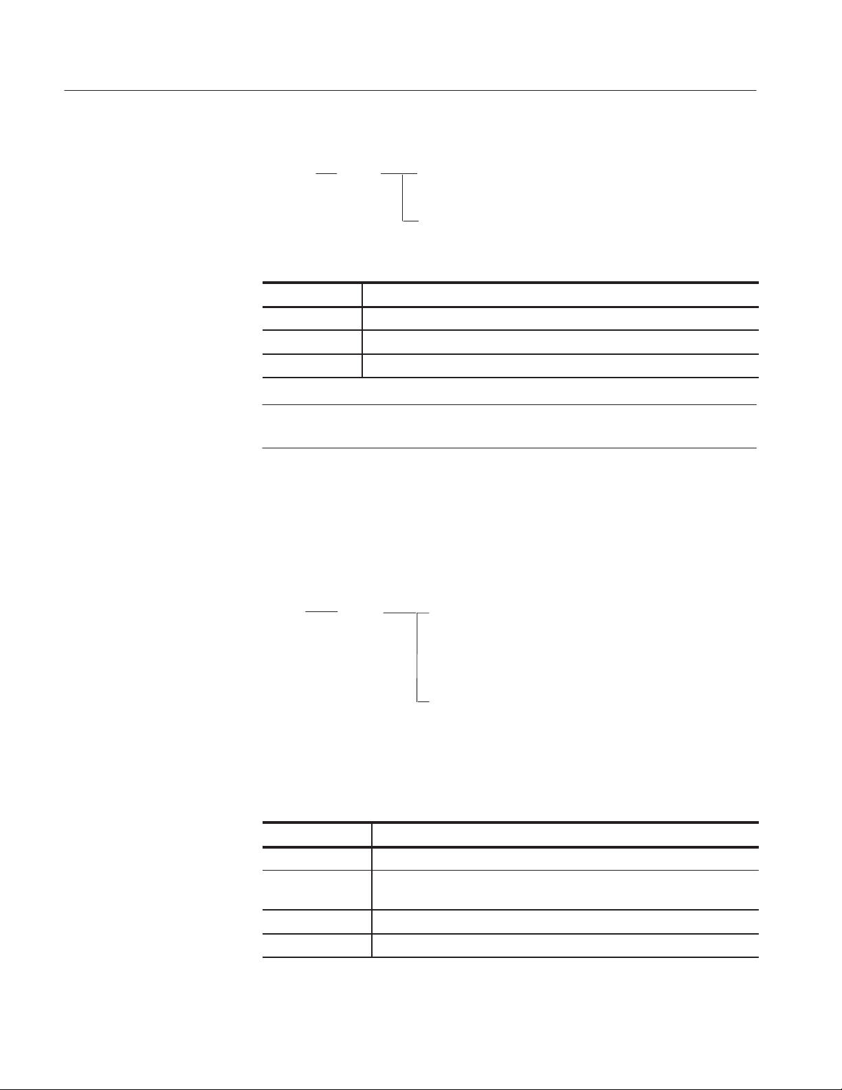
Selecting Measurements
The next figure shows how to access the selections in the Select Measurement
side menu, and Table 2–6 lists the measurements with a brief description of each.
NOTE. You can choose the Clear All Selected side menu item to remove all the
measurements in the Select Active Measurements menu.
offers seven color themes
2–4
TDSJIT1V2 Jitter Analysis Application User Manual
Page 30
Basic Operations
Main menu Side menu
Meas
Setup
Select
Measurement
Side menu
General
Clock
Data
Clock-Data
Ch-Ch
Side menu items
Rise Time
Fall Time
Positive Width
Negative Width
High Time
Low Time
Data Frequency
Data Period
Data TIE
Setup Time
Hold Time
Clock Out Time
Skew
Clock Frequency
Clock Period
Cycle-Cycle Period
N-Cycle Period
Positive Cy-Cy Duty
Negative Cy-Cy Duty
Positive Duty Cycle
Negative Duty Cycle
Clock TIE
T able 2–6: Select Measurement menu selections
Group Selection Description
General Rise Time Elapsed time from when a rising edge crosses the low reference voltage level and
then the high reference voltage level
Fall Time Elapsed time from when a falling edge crosses the high reference voltage level and
then the low reference voltage level
Positive Width Difference in time between the leading edge and trailing edge of a pulse
Negative Width Difference in time between the trailing edge and leading edge of a pulse
High Time Amount of time a waveform remains above the high reference voltage level
Low Time Amount of time a waveform remains below the low reference voltage level
Clock Clock Period* Elapsed time between when a waveform crosses a specific reference voltage level
twice
Clock Frequency* Inverse of the period for each clock cycle
Cycle-Cycle Period* Difference in period measurements from one cycle to the next
N-Cycle Period* Difference in period measurements from cycles between two consecutive groups of
N-cycles where N is any number
Positive Cy-Cy Duty Difference between two consecutive positive widths
Negative Cy-Cy Duty Difference between two consecutive negative widths
Positive Duty Cycle* Ratio of the positive portion of the cycle relative to the period
Negative Duty Cycle* Ratio of the negative portion of the cycle relative to the period
Clock TIE* Difference in time between the designated edge on a sampled clock waveform to
the designated edge on a calculated clock waveform with a constant frequency
(zero jitter)
Data Data Period Elapsed time between when a waveform crosses a specific reference voltage level
in the same direction twice
Data Frequency Inverse of the period for each data cycle
TDSJIT1V2 Jitter Analysis Application User Manual
2–5
Page 31
Basic Operations
T able 2–6: Select Measurement menu selections (Cont.)
Group DescriptionSelection
Data TIE Difference in time between the data edges on a sampled data waveform to the data
edges on a calculated data waveform with a constant rate (zero jitter)
Clock-Data Setup Time* Elapsed time between when a data waveform crosses a voltage reference level
followed by the clock signal crossing its own voltage level
Hold Time* Elapsed time between when the clock waveform crosses a voltage reference level
followed by a data waveform crossing its own voltage level
Clock Out Time* Elapsed time between when the clock waveform crosses a voltage reference level
followed by an output waveform crossing its own voltage level
Ch-Ch Skew* Difference in time between the designated edge on a principal waveform to the
designated edge on another waveform
* Requires configuration.
Selecting a Measurement
to Configure
Configuring a Measurement
You may need to configure one or more of the selected measurements. The next
figure shows how to select the measurement for configuration.
Many measurements require configuration, as indicated in Table 2–7. The next
figure shows how to access the Configure Selected menu for each measurement.
Main menu Side menu
Meas
Setup
Select Active
Measurement
GP
Table 2–7 lists the measurements and configuration selections with a brief
description of each. Refer to the Parameters section for default values.
T able 2–7: Measurements and configuration selections
Measurement Selection Description
Rise Time, Fall Time, Positive
Width, Negative Width, High TIme,
Low Time, Positive Cy-Cy Duty ,
Negative Cy-Cy Duty, Data Period,
Data Frequency, Data TIE
None No configuration is required for these measurements
Use GP knob to scroll through
list of selected measurements
Side menu
Configure
Selected
Clock Frequency , Clock Period,
Cycle-Cycle Period, Positive Duty
Cycle, Negative Duty Cycle, and
Clock TIE, N-Cycle Period, Setup
Time, Hold Time, Clock Out Time
2–6
Common Cycle Start Edge
Defines which edge of the Main input is used to calculate all active
clock-based measurements
TDSJIT1V2 Jitter Analysis Application User Manual
Page 32

T able 2–7: Measurements and configuration selections (Cont.)
Measurement DescriptionSelection
N-Cycle Period Cycle Span N=
Number of cycles between cycles actually measured
Basic Operations
Meas Made Every
Start Meas at Cycle #
Setup Time, Hold Time,
Clock Out Time
Skew From Edge
* Although you can enter the same values for the Range Max and Range Min side menu items, the application requires that
they always be at least one resolution apart. The application displays the actual value for Range Max or Range Min,
whichever was last selected, in the upper right corner of the display.
Specifying Inputs
Common Data Cycle Edge
Range Max*
Range Min*
To Edge
Range Max*
Range Min*
The application takes measurements from waveforms specified as inputs.
Specifies if the measurement is taken on all 2N groups (option 1) or
on every Nth 2N group (option N)
Number of cycles skipped prior to starting the measurement
Edge on the data waveform used to take the measurement; you
can define the waveform in the Inputs: 2nd menu
Specify the maximum range of valid measurement values
Specify the minimum range of valid measurement values
Edge on the Main waveform used to take the measurement
Edge on the 2nd waveform used to take the measurement
Specify the maximum range of valid measurement values
Specify the minimum range of valid measurement values
NOTE. All General, Clock, and Data measurements require a Main input.
All Clock-Data and Ch-Ch measurements require a Main input and a 2nd input.
The next figure shows how to access parameters in the Main Input and 2nd Input
menus.
Main menu Side menu Side menu items
Inputs
*Only available for the Main Input.
Main or
2nd
NOTE. The Input Summary shows the settings of all the Input menus.
TDSJIT1V2 Jitter Analysis Application User Manual
Source
Autoset Ref Levels
Vertical Autoset
Mid Ref
High Ref*
Low Ref*
Hysteresis
2–7
Page 33

Basic Operations
Table 2–8 lists the Main Input and 2nd Input menu selections with a brief
description of each.
T able 2–8: Main Input and 2nd Input menus selections
Selection Description
Source Sets which waveform the application uses as the signal or clock source
Autoset Ref Levels Refer to Table 2–9
Vertical Autoset Changes the vertical scale and position for Ch 1, Ch 2, Ch 3, and Ch 4
waveforms so that they occupy the full vertical space available on the
display without any part of the waveform missing (clipped)
Mid Ref Sets the middle threshold level on the slope, in volts; refer to Figure 2–2
High Ref* Sets the high threshold level on the slope, in volts; refer to Figure 2–2
Low Ref* Sets the low threshold level on the slope, in volts; refer to Figure 2–2
Hysteresis Sets the threshold margin, in volts, relative to the reference level which
the voltage must cross to be recognized as changing; the margin is the
voltage reference level plus or minus half the hysteresis
*Only available for the waveform defined in the Main Input menu.
High
Mid
Low
NOTE. The application detects the minimum and maximum voltage levels of the
waveform. If the reference voltage level plus or minus the hysteresis falls outside
of 2.5% to 97.5% of the waveform peak-to-peak range, no measurement is taken.
Figure 2–2 shows how to determine the voltage reference levels.
Mid
Main Input reference levels
2nd Input and Qualifier Input reference level
Figure 2–2: How to determine voltage reference levels
Autoset Ref Levels Menu. Autoset is only valid when Ch1, Ch2, Ch3, or Ch4 are
selected as the Source for the Main Input, 2nd Input, or Qualifier Input menus.
The next figure shows how to access parameters in the Autoset Ref Levels
menus.
2–8
TDSJIT1V2 Jitter Analysis Application User Manual
Page 34

Basic Operations
Side menu Side menu items
Autoset Ref Levels
*Only available for the Main Input.
Mid Ref
High Ref*
Low Ref*
Hysteresis
Perform Autoset
Table 2–9 lists the Autoset Ref Levels menu selections with a brief description
of each. The Autoset Ref Levels function is only valid for signals on Ch1, Ch2,
Ch3, and Ch4.
T able 2–9: Autoset Ref Levels menu selections
Selection Description
Mid Ref Sets the middle threshold level as a percentage of the voltage levels relative
to the minimum and maximum levels of the peak-to-peak values
High Ref* Sets the high threshold level as a percentage of the voltage levels relative to
the minimum and maximum levels of the peak-to-peak values
Low Ref* Sets the low threshold level as a percentage of the voltage levels relative to
the minimum and maximum levels of the peak-to-peak values
Hysteresis Sets the threshold margin as a percentage of the voltage levels relative to
the reference level which the voltage must cross to be recognized as
changing; the margin is the voltage reference level plus or minus half the
hysteresis
Perform Autoset Calculates and sets the threshold levels and margin
*Only available for the waveform defined in the Main Input menu.
NOTE. If you perform an Autoset on Ch1, Ch2, Ch3, or Ch4 and then change the
Source to a reference memory or math waveform, the application will retain the
previous Autoset reference level values. If the values are not appropriate, you
must set the values for the voltage reference levels and hysteresis manually.
Deskew Menu. The next figure shows how to access parameters in the Deskew
menu and Table 2–10 lists the setup parameters with a brief description of each.
TDSJIT1V2 Jitter Analysis Application User Manual
2–9
Page 35
Basic Operations
Specifying Qualifiers
Side menu
2nd Input
Side menu
Deskew
Side menu items
Upper Range
Lower Range
Perform Deskew
T able 2–10: Deskew menu selections
Selection Description
Upper Range Specifies the upper range of valid measurement values
Lower Range Specifies the lower range of valid measurement values
Perform Deskew Starts the Deskew utility
NOTE. To deskew the probes and oscilloscope channels, refer to Deskewing the
Probes and Channels starting on page 1–4.
Qualifiers allow you to focus the application on more narrowly defined
conditions before taking measurements. This is one way to filter out information
that is not useful to analyze.
Main menu Side menu Side menu items
Inputs
Qualifier
On/Off
Valid When
Source
Mid Ref
Hysteresis
Autoset Ref Levels
Table 2–11 lists the Qualifier Input menu selections with a brief description of
each.
T able 2–11: Qualifier Input menu selections
Selection Description
On/Off Enables the qualifier
Valid When Specifies the state condition of the qualifier that must be met as either a
logical low (0) or a logical high (1)
Source Sets which waveform the application uses as the qualifier source
Mid Ref Sets the middle threshold level on the slope, in volts; refer to Figure 2–2
2–10
TDSJIT1V2 Jitter Analysis Application User Manual
Page 36

Basic Operations
T able 2–11: Qualifier Input menu selections (Cont.)
Selection Description
Hysteresis Sets the threshold margin, in volts, relative to the reference level which
the voltage must cross to be recognized as changing; the margin is the
voltage reference level plus or minus half the hysteresis
Autoset Ref Levels Refer to Table 2–9
NOTE. The Qualifier Input and Gating functions are mutually exclusive. If you
enable both, the application displays an error message.
Specifying Gating
Using Horizontal Check
Gating allows you to focus the application on a specific area of the waveform
bound by cursors before taking measurements. This is one way to filter out
information that is not useful to analyze.
Main menu Side menu
Inputs
Gating: On/Off
NOTE. Disabling the V Bars Cursors on the oscilloscope causes the application
to disable Gating although the application display will show that gating is On.
You can use the Horizontal Check to check if the Sample Rate is appropriate for
the selected measurements. A message displays that tells you if the Sample Rate
is appropriate for the Main Input or 2nd Input menus. Accurate measurements
require at least two samples per edge. The next figure shows how to access this
function.
Main menu Side menu
Inputs
Horizontal Check
Using Acquisition Timeout
You can use the Acquisition Timeout to set an appropriate amount of time that
the application will wait to acquire data before it stops and displays an error
message. The next figure shows how to access this function.
TDSJIT1V2 Jitter Analysis Application User Manual
2–11
Page 37

Basic Operations
Taking Measurements
Main menu Side menu
Inputs
Acquisition Timeout
Side menu items
Acquisition Timeout
Timeout
Auto
User
T able 2–12: Acquisition Timeout menu selections
Selection Description
Acq Timeout Auto sets the timeout to less than 0.1 hours; User allows you to enter a
larger timeout value
Timeout When User is selected, you can set the timeout from 0.1 hour to 24 hours
If you want to change trigger settings or localize the measurement, you should
do so before you take any measurements.
NOTE. If you select a reference or math waveform as the source, you will need to
recall and display the waveform before the application can take a measurement.
For information on how to recall a waveform, refer to Recalling a Waveform
File on page 2–29. To display the waveform, press the MORE button and the
appropriate main menu item.
Acquiring Data
Be sure to press Control (main) ➞ Reset Results (side) to reset the result values
if you change the Vertical or Horizontal time settings between measurements.
You can start the application and oscilloscope to acquire data and take measurements through the Control menu. The next figure shows how to access parameters in the Control menu.
Main menu Side menu Side menu items
Control
Mode
Start/Continue
Pause
Stop
Reset Results
Single
Free Run
Single No Acq
To take measurements from displayed waveforms, follow these steps:
1. Press Control (main). Table 2–13 lists selections in the Control menu.
2–12
TDSJIT1V2 Jitter Analysis Application User Manual
Page 38

Basic Operations
T able 2–13: Control menu selections
Selection Description
Mode
Single
Free Run Repeatedly acquires the input waveform(s) and takes measurements
Single No Acq Performs measurements on a previous acquisition and then stops
Performs measurements on a single acquisition and stops
Start
Continue
Pause The application pauses and resumes when you press Continue or stops
Stop The application stops taking measurements
Reset Results Resets all result values to zero; data log files have their own reset selection
The application starts to take measurements from the waveform(s)
When paused, the application continues taking measurements
when you press Stop
NOTE. Acquisition Timeout causes the application to stop after a specific amount
of time has elapsed when acquiring data and taking measurements. If you
change any oscilloscope settings, be sure to reset the results.
2. Press Mode (side) to select Single or Free Run acquisition mode.
3. Press Start (side).
NOTE. Do not change oscilloscope settings while a measurement is being taken,
since this can cause an invalid measurement.
Localizing Measurements
You can control the amount of data to measure by adjusting the Record Length,
or the Trigger Position. By specifying the Trigger Position, the starting point,
and the total length of the measurement, you can effectively size the area of
interest.
NOTE. If an error message displays because ther e are not enough cycles from
which to take a measurement, you should increase the Record Length.
Be sure to reset the results each time you change the Record Length or other
oscilloscope settings.
TDSJIT1V2 Jitter Analysis Application User Manual
2–13
Page 39
Basic Operations
Warning Messages
The application displays and saves warning messages if the input conditions do
not support accurate measurements. You can view the most recent message, if
any, for the current acquisition in the Results menu or the Plots menu. The next
figure shows how to access warning messages.
Analyzing the Results
Main menu
Results
Plots
Side menu
Warning
Warning
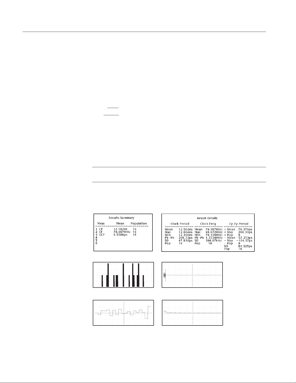
The application provides information on the variation of timing measurements as
statistical values in a readout, or graphically as a Histogram, Time Trend, Cycle
Trend, or Spectrum plot.
NOTE. Stop the acquisition before viewing the results as plots if you are taking
measurements in the Free Run mode.
Figure 2–3 shows an example of the various results display formats.
Results Summary
Results Detail
2–14
Histogram plot
Time Trend plot Spectrum plot
Cycle Trend plot
Figure 2–3: Example of the results and display formats
TDSJIT1V2 Jitter Analysis Application User Manual
Page 40
Basic Operations
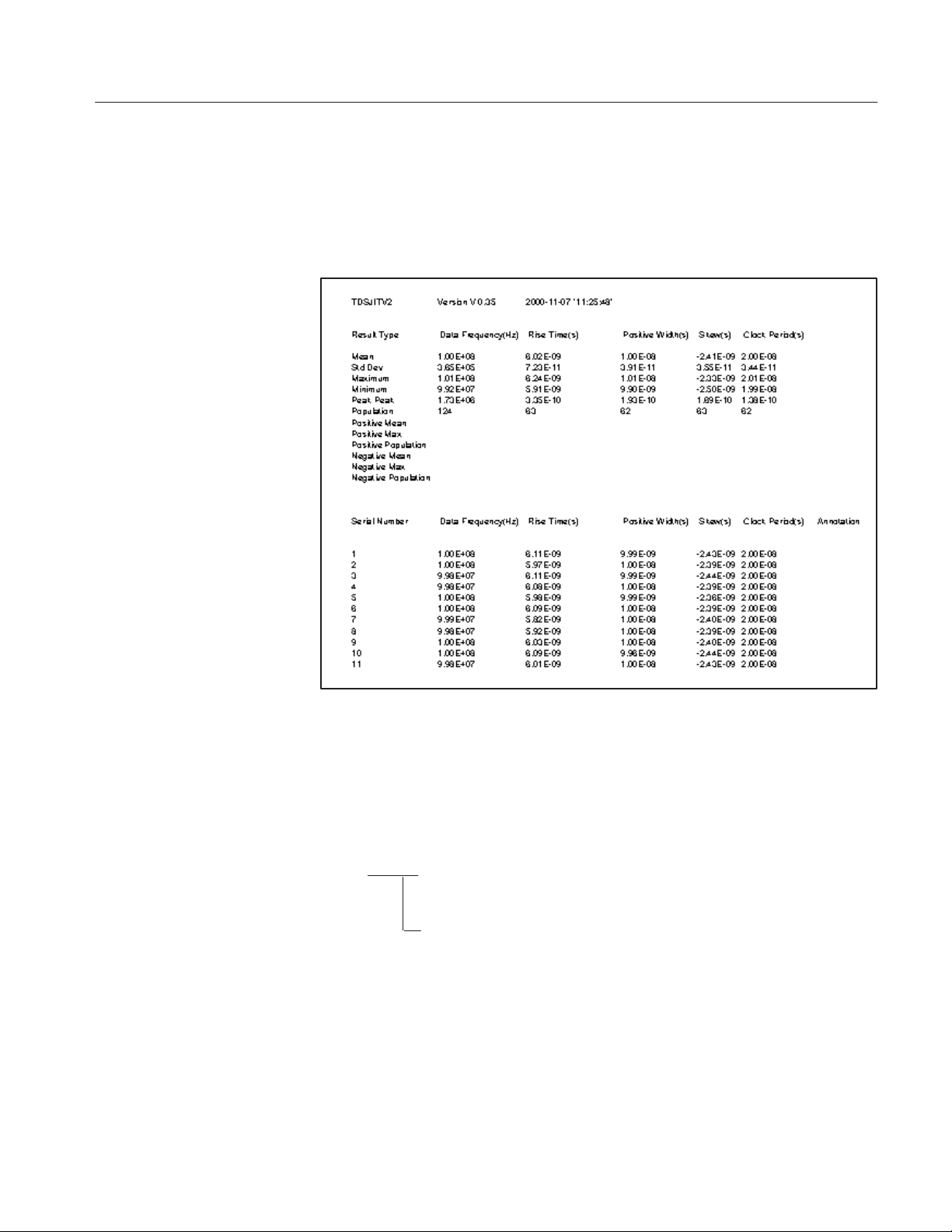
You can also log the data to a RESULTS.CSV file for viewing with a text
editing, spreadsheet, database, or data analysis program on a personal computer.
Figure 2–4 shows an example of how the RESULTS.CSV file might look in a
spreadsheet.
Figure 2–4: A RESULTS.CSV file viewed in a spreadsheet program
Viewing Statistics
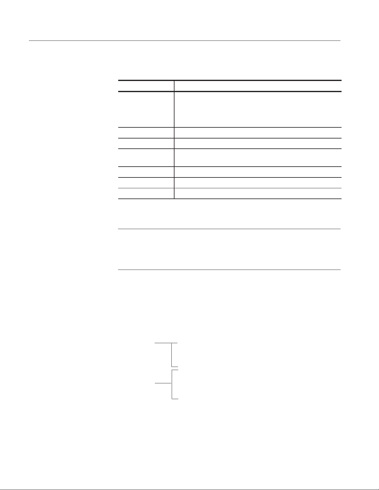
The application can display results for up to six measurements. The next figure
shows how to access the Summary, Details, and Warnings message boxes.
Main menu
Results
Side menu
Summary
Details
Warnings
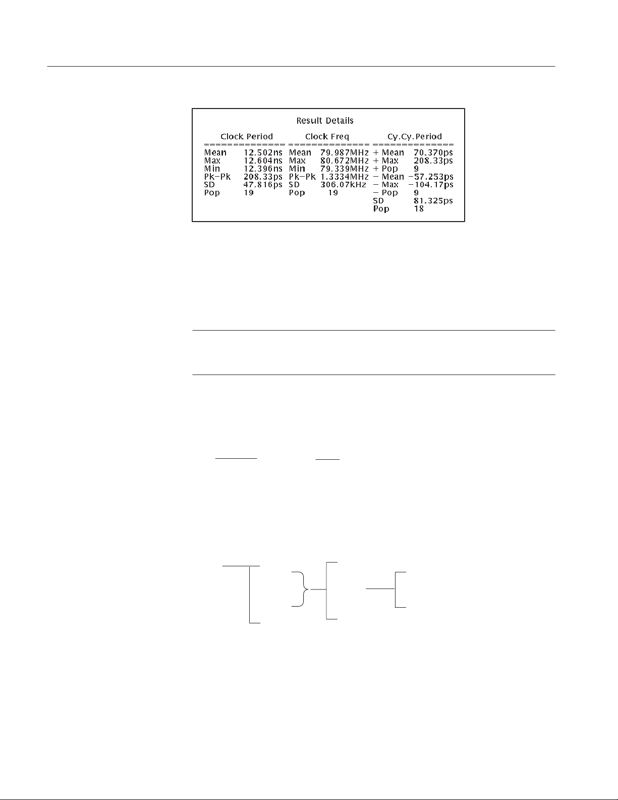
The statistical information that displays will vary by measurement. In general,
the Summary and Details message boxes contain statistical values for the mean,
the standard deviation (StdDev), the peak-to-peak (Pk-Pk), the maximum (Max)
and minimum (Min) values, and the population (the number of samples used to
calculate the statistics).
Figure 2–5 shows an example of the results for three measurements.
TDSJIT1V2 Jitter Analysis Application User Manual
2–15
Page 41
Basic Operations
Figure 2–5: Results Details menu, example of three measurements
To view parts of the waveform that are obscured by the statistics, press the
CLEAR MENU button. To return to the application, press the SHIFT, and then
the APPLICATION front-panel menu buttons
NOTE. To view the waveform and the results, you can adjust the placement of the
statistics in the display or make dialog boxes translucent through the Display
Options side menu.
Viewing Plots
The next figure shows how to make the statistics and all dialog boxes visible or
invisible.
Main menu Side menu Side menu item
Utility
Display Options
Dialog Box: On/Off
You can graphically plot the results for easier analysis. There are four plot
formats: Histogram, Time Trend, Cycle Trend, and Spectrum. The next figure
shows how to access the Plots menus.
Main menu
Plots
Side menu
Ref1 Plot
Ref2 Plot
Ref3 Plot
Ref4 Plot
Warning
On/Off
Active Meas
Plot Type
Vert/Horiz Axis
Spectrum
Histogram
Cycle Trend
Time Trend (and Spectrum)
Table 2–14 lists the plot formats with a brief description of each.
2–16
TDSJIT1V2 Jitter Analysis Application User Manual
Page 42

Basic Operations
T able 2–14: Plot Type selections
Selection Description
Histogram Plots the results such that the horizontal axis represents the measurement
values and the vertical axis represents the number of times that the value
occurred
Cycle Trend Plots the results such that the vertical axis represents the measurement
value and the horizontal axis represents the index number of the
measurement which can be used to observe the variation of a measurement
Time Trend* Plots the results such that the vertical axis represents the measurement
value and the horizontal axis represents the time the measurement
occurred; the horizontal time span is the same as the input waveform
Spectrum** Plots the spectral content (FFT) of the Time Trend plot where the vertical
axis represents magnitude and the horizontal axis represents frequency
* Limited to a 50,000 point record length; if the plot exceeds this limit, use Decimation.
** Limited to a 10,000 point record length; if the plot exceeds this limit, use Decimation.
NOTE. You must take a measurement before displaying the results as a plot. The
application will automatically display a plot when it is enabled.
Be sure to reset the results each time you change oscilloscope settings.
The next figure shows how to select an active measurement to display as a plot.
Side menu Side menu item
Ref# Plot
Active Meas
Use knob to cycle through
selected measurements
GP
Vert/Horiz Axis for a Histogram Plot. The next figure shows how to access the
Vert/Horiz Axis parameters for a Histogram plot.
Side menu Side menu item
Vert/Horiz Axis
Histogram
Autoset
Center
Span
Bin Resolution
Scale
Vertical Height
Refresh
Table 2–15 lists the Vert/Horiz Axis parameters for a Histogram plot with a brief
description of each.
TDSJIT1V2 Jitter Analysis Application User Manual
2–17
Page 43
Basic Operations
T able 2–15: Vert/Horiz Axis Histogram menu selections
Selection Description
Autoset* Uses the results to determine logical values for the Center and Span
parameters if the population of the measurement is 3 or more, and
redraws the plot in the corresponding reference memory
After using Autoset, the oscilloscope cursors are not available
Center Numeric value for the horizontal center position of the histogram
Span Numeric value for the total horizontal range of the histogram
Bin resolution Selects the resolution as defined by bins to be Low (20 bins), Medium
(100 bins), or High (500 bins)
Scale Vertical axis is in logarithmic or in linear scale
Vertical Height Height of the plot in number of divisions
Refresh Updates the plot with the latest Center and Span values entered
*You must select On for the Ref# Plot that will store the Histogram and take a measurement before using Autoset.
NOTE. Use the HORIZONTAL SCALE knob to adjust the horizontal scale of the
waveform to fit the screen for proper viewing.
Use the Autoset function to set the optimum Center and Span values. You can use
Autoset only after taking measurements and storing them as a Histogram plot.
Vert/Horiz Axis for a T ime Trend and Spectrum Plots. The next figure shows how to
access the Vert/Horiz Axis parameters for a Time Trend plot, and how to access
the Spectrum plot.
Side menu
Vert/Horiz Axis
Time Trend
Spectrum
Side menu items
Vertical Height
Decimation
Length
State
Destination
Scale
Window
2–18
TDSJIT1V2 Jitter Analysis Application User Manual
Page 44

Basic Operations
NOTE. The Time Trend plot is limited to a 50,000 point record length; the
Spectrum plot is limited to a 10,000 point record length. If the record length
exceeds these limits, use Decimation to plot the results with fewer samples.
Table 2–16 lists the Vert/Horiz Axis parameters for a Time Trend plot with a
brief description of each.
T able 2–16: Vert/Horiz Axis Time Trend menu selection
Selection Description
Vertical Height Height of the plot in number of divisions
Decimation Produces a waveform with fewer samples than in the original acquisition
Length For decimation, the length of the plot in number of record points
To view the results in a Time Trend plot, follow these steps:
1. Take jitter measurements.
2. If the record length is greater than 50,000 points, enable Decimation and
select an appropriate value for the Length side menu item.
3. Enable the Time Trend plot; the application automatically displays the plot.
Table 2–17 lists the parameters for a Spectrum plot with a brief description of
each.
T able 2–17: Spectrum menu selection
State Enables the application to plot the results as a spectrum
Destination Sets the Math1, Math2, or Math3 waveform in which to store the plot
Scale Vertical axis is in logarithmic or in linear scale
Window Reduces spectral leakage in the Fast Fourier Transform (FFT)
waveform; a Hanning window (raised cosine) on the Time Trend data
To view the results in a Spectrum plot, follow these steps:
1. Take jitter measurements.
2. If the record length is equal to or less than 10,000 points, go to step 3.
If the record length is greater than 10,000 points, enable Decimation and
select an appropriate value for the Length side menu item that is equal to or
less than 10,000 points.
TDSJIT1V2 Jitter Analysis Application User Manual
2–19
Page 45

Basic Operations
3. Enable the Time Trend plot; the application automatically displays the plot.
4. Enable the Spectrum plot; the application automatically displays the plot in
the MORE menu of the oscilloscope.
5. To return to the application, press the SHIFT, and then the APPLICATION
front-panel menu buttons.
Vert/Horiz Axis for a Cycle Trend Plot. The next figure shows how to access the
Vert/Horiz Axis parameters for a Cycle Trend plot.
Clearing Results
Side menu
Vert/Horiz Axis
Cycle Trend
Side menu items
Vertical Height
Decimation
Length
Table 2–18 lists the Vert/Horiz Axis parameters for a Cycle Trend plot with a
brief description of each.
T able 2–18: Vert/Horiz Axis Cycle Trend menu selections
Selection Description
Vertical Height Height of the plot in number of divisions
Decimation Produces a waveform with fewer samples than in the original acquisition
Length For decimation, the length of the plot in number of record points
To reset the results to zero, press Control (main) ➞ Reset Results (side). You do
not have to wait for a measurement to complete to clear the results.
Saving the Results to a File
You can save the results for all active measurements as statistics to a data log file
or save the minimum and maximum worst case waveforms to waveform files.
You can also change the active measurements and continue to log data to the
same data log file.
Logging Statistics
2–20
This type of logging saves the statistical results and the individual result points
of activated measurements to a data log file. The next figure shows how to
access the Log Results menu.
TDSJIT1V2 Jitter Analysis Application User Manual
Page 46

Basic Operations
Log
Side menu
Results
Side menu itemsMain menu
On/Off
Store Results In
Clear Log File
Log Directory
Select Drive
Table 2–19 lists the Log Results menu selections with a brief description of each.
T able 2–19: Log Results menu selections
Selection Description
On/Off Enables or disables the data log file; when enabled, stores the measure-
ment results in a “comma separated variable” formatted file (.CSV file) that
you can view on a personal computer
Store Results In Allows you to enter a name for the .CSV file
Clear Log File Clears the data log file; you must disable the log file before you can clear its
contents
Log Directory Selects the directory in which the .CSV file will be saved; when you select
this side menu item, the directory structure of the selected drive displays.
Select Drive Selects the drive on which the .CSV file will be stored
Data Log File Format
NOTE. If the disk is full or not present, the application displays an error message
and stops taking measurements.
A data log file larger than 1.4 MB exceeds the capacity of a floppy disk. Refer to
Appendix D: Example Program to Copy Large Files for an example of a GPIB
program that you can use to transfer a large data log file from the oscilloscope
to a personal computer.
The data log file contains three parts: a header row, statistical results, and
individual result points. The header row of the log file contains the application
name, the version number of the application, and the date and time on which the
file was created.
For statistical results, the application updates the rows for all of the active
measurements. For individual result points, the application appends rows of
results to each active measurement.
TDSJIT1V2 Jitter Analysis Application User Manual
2–21
Page 47

Basic Operations
NOTE. If you are using a GPIB program to execute the application, such as in
automated test environments, you can add your own annotation through the
logAnnotate GPIB command. You can add information consisting of up to 20
characters; the custom information will appear as the last column in the
individual result records of that acquisition.
Logging Min/Max
Waveforms
This type of logging saves the acquired waveforms where the minimum and
maximum worst cases occur. When enabled, the waveforms are saved to a set of
.wfm files that are stored with the other application files.
The next figure shows how to access the Log Min/Max Wfms menu.
Main menu
Log
Side menu
Min/Max Wfms
Side menu items
On/Off
Min/Max Directory
Table 2–20 lists the Log Min/Max Wfms menu selections with a brief description of each.
T able 2–20: Log Min/Max Wfms menu selections
Selection Description
On/Off Enables the saving of worst case waveforms; see Table 2–21 for
definition
Min/Max Directory Changes the directory in which .wfm files will be stored
2–22
NOTE. File names for the waveforms are unique to each measurement. The Min1
and Max1 waveform files are for the Main input. The Min2 and Max2 waveform
files are for the 2nd input.
Table 2–21 lists the file names of the minimum and maximum worst case
waveforms for various measurements.
T able 2–21: File names for Min/Max waveforms
Measurement Min waveform Max waveform
Rise Time RISEMin1.wfm RISEMax1.wfm
Fall Time FALLMin1.wfm FALLMax1.wfm
Positive Width PWMin1.wfm PWMax1.wfm
TDSJIT1V2 Jitter Analysis Application User Manual
Page 48

Basic Operations
T able 2–21: File names for Min/Max waveforms (Cont.)
Measurement Max waveformMin waveform
Negative Width NWMin1.wfm NWMax1.wfm
High Time HIGHMin1.wfm HIGHMax1.wfm
Low Time LOWMin1.wfm LOWMax1.wfm
Clock Frequency CFMin1.wfm CFMax1.wfm
Clock Period CPMin1.wfm CPMax1.wfm
Cycle-Cycle Period CCPMin1.wfm CCPMax1.wfm
N-Cycle Period NCPMin1.wfm NCPMax1.wfm
Positive Cy-Cy Duty PCCDMin1.wfm PCCDMax1.wfm
Negative Cy-Cy Duty NCCDMin1.wfm NCCDMax1.wfm
Positive Duty Cycle PDCMin1.wfm PDCMax1.wfm
Negative Duty Cycle NDCMin1.wfm NDCMax1.wfm
Clock TIE TIEMin1.wfm TIEMax1.wfm
Data Frequency DFMin1.wfm DFMax1.wfm
Data Period DPMin1.wfm DPMax1.wfm
Data TIE DTIEMin1.wfm DTIEMax1.wfm
Setup Time SUMin1.wfm
SUMin2.wfm
Hold Time HOLDMin1.wfm
HOLDMin2.wfm
Clock Out Time TCOMin1.wfm
TCOMin2.wfm
Skew Time SKEWMin1.wfm
SKEWMin2.wfm
Importing a Data Log File to a Personal Computer
You can import the .CSV data log file (comma separated variable format) into a
text editing, spreadsheet, database, or data analysis program on your personal
computer for further analysis.
If you saved the data log file on the hard disk drive, you need to copy it to a
floppy disk. To do so, follow these steps:
SUMax1.wfm
SUMax2.wfm
HOLDMax1.wfm
HOLDMax2.wfm
TCOMax1.wfm
TCOMax2.wfm
SKEWMax1.wfm
SKEWMax2.wfm
1. Insert a blank, DOS-formatted floppy disk into the floppy disk drive of the
oscilloscope.
TDSJIT1V2 Jitter Analysis Application User Manual
2–23
Page 49

Basic Operations
2. Copy the .CSV file from the hard disk drive to the floppy disk. For details
on how to do this, refer to step 5 on page 2–41 in the Tutorial section.
To import a data log file to a personal computer, follow these steps:
1. Insert the floppy disk into the floppy disk drive on your personal computer.
2. Copy the .CSV file.
3. Open the file using a text editing, spreadsheet, database, or data analysis
program.
Figure 2–4 shows an example of the .CSV file viewed in a spreadsheet program.
If you take different measurements and store them in one data log file, you can
group the measurements by sorting them in a program on a personal computer.
Saving and Recalling Setups
You can use the Save/Recall Setup menu to save and recall application setups.
The Save/Recall function also saves the oscilloscope set up.
Saving a Setup
The next figure shows how to access the Save/Recall Setup menu.
Main menu Side menu Side menu item
Utility Save/Recall Setup
Save Name
Save Setup
Recall Name
Recall Setup
To save the application setup to the file displayed in the Save Name menu item,
press Save Setup (side).
To create a new file in which to save the application setup, follow these steps:
1. Press Save Name (side).
2. Use the direction arrows and Delete Char (side) to clear the existing file
name or part of the file name.
3. Use the General Purpose (GP) knob to select each character in the file name.
Press Enter Char (side) after selecting each character.
The file name can be up to eight characters long excluding the extension.
The application automatically appends a .ini and .set extension to the name.
2–24
4. Press OK Accept (side) to save the file name.
5. Press Save Setup (side) to store the application setup in the file just created.
TDSJIT1V2 Jitter Analysis Application User Manual
Page 50

Basic Operations
6. Press OK (side).
7. Done (side).
Application setups are usually saved in the APPS/TDSJIT1V2/TEMP directory
(accessed through the File Utilities menu) on the oscilloscope. Once you have
saved a setup, you must recall it to use it again.
Recalling a Setup
Exiting the Application
To recall the application settings from the Default setup file or from a saved
setup file, follow these steps:
1. Press Recall Name (side); use the GP knob to select the directory where the
setup file resides.
NOTE. The application starts with all parameters set to default values regardless
of which setup file was last used.
2. When you have found the setup file to recall, press Recall Setup (side).
3. Press OK (side).
4. Press Done (side).
To exit the application, press Utility (main) ➞ Exit (side). To confirm, press
OK (side).
TDSJIT1V2 Jitter Analysis Application User Manual
2–25
Page 51

Basic Operations
2–26
TDSJIT1V2 Jitter Analysis Application User Manual
Page 52

Tutorial
This tutorial teaches you how to set up the application, take two types of
measurements, and view the results in the various formats. Further operating
information is located in the Operating Basics section.
Before you begin the tutorial, you must do the following tasks:
H Set up the oscilloscope
H Start the application
H Recalling waveforms to reference memories
Setting Up the Oscilloscope
To set up the oscilloscope, follow these steps:
1. Press SETUP ➞ Recall Factory Setup (main) ➞ OK Confirm Factory Init
(side) to set the oscilloscope to the default factory settings.
2. Press the WAVEFORM OFF button as often as necessary to remove active
waveforms from the display.
Starting the Application
3. Press HORIZONTAL MENU ➞ –more– 1 of 3 (side) ➞ 5000 points in
100 divs (side) to set the Record Length to 5000.
To perform these lessons, the TDSJIT1V2 application must be installed on the
oscilloscope. See Installation on page 1–3.
To start the application, refer to Figure 2–6, and follow these steps:
1. Press SETUP ➞ Select Application (main).
2. Use the general purpose (GP) knob to select hd0: and press SELECT.
3. Use the GP knob to select the TDSJIT1V2.APP file and press Activate
Application (side).
The application starts up and displays as shown in Figure 2–7.
TDSJIT1V2 Jitter Analysis Application User Manual
2–27
Page 53

Tutorial
Figure 2–6: Starting the application
2–28
Figure 2–7: TDSJIT1V2 application initial display
TDSJIT1V2 Jitter Analysis Application User Manual
Page 54

Recalling a Waveform File
The application includes waveform files for use with this tutorial. Table 2–22
shows the types of signals that these waveforms represent and the reference
memory that you will recall them to.
T able 2–22: Tutorial waveforms and signal types
Waveform name Signal type Recall to reference
J1V2_CLK.WFM A clock signal Ref4
J1V2_DAT.WFM A data signal Ref3
To recall the clock waveform to Ref1, follow these steps:
1. Press WAVEFORM ➞ Recall Wfm to Ref (main) ➞ Recall from file (side).
2. Use the general purpose (GP) knob to select hd0: and press SELECT.
Tutorial
3. Use the GP knob to select WFMS and press SELECT.
4. Use the GP knob to select J1V2_CLK.WFM; press To Ref4 active/empty
(side). Figure 2–8 shows how to recall a waveform.
Figure 2–8: Recalling a waveform to a reference memory
TDSJIT1V2 Jitter Analysis Application User Manual
2–29
Page 55
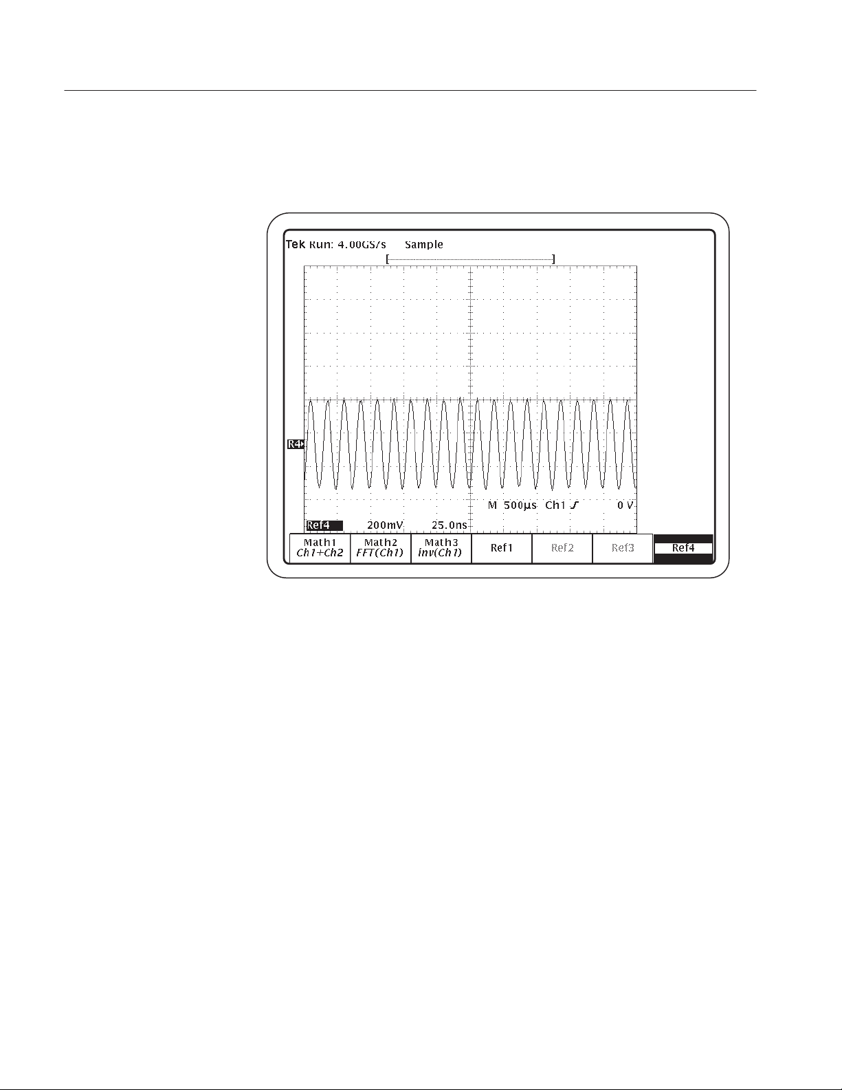
Tutorial
5. Press the MORE front-panel button, and then Ref4 (main) to display the
waveform. Figure 2–9 shows the J1V2_CLK.WFM recalled to Ref4.
Figure 2–9: J1V2_CLK.WFM recalled to Ref1
6. Press the SHIFT, and then the APPLICATION front-panel menu button to
return to the application.
Taking a Clock Period Measurement
In this example, you will learn how to use the application to take a Clock Period
measurement, how to view the results as statistics, and how to view the results in
the various plot formats.
To take a Clock Period measurement, follow these steps:
1. Select Inputs (main) ➞ Main (side) ➞ Source (side) ➞ –more– 1 of 4
(side) ➞ –more– 2 of 4 (side) ➞ Ref4 (side). Figure 2–10 shows the Main
Input menu setup.
2–30
TDSJIT1V2 Jitter Analysis Application User Manual
Page 56

Tutorial
Figure 2–10: Main Input menu setup
2. Press Done (side) twice.
3. To take the measurement, press Control (main) ➞ Start (side).
NOTE. When the input is a reference waveform, the measurement performs a
single measurement cycle regardless of the acquisition mode.
The Control menu (main) displays Control Sequencing while the application
is executing. When the Control menu displays Control Ready, the application has completed the calculations.
4. Wait for the calculations to complete. Figure 2–11 shows the results.
TDSJIT1V2 Jitter Analysis Application User Manual
2–31
Page 57

Tutorial
Figure 2–11: Clock Period lesson: Results Summary readout
5. To set up the Histogram plot format, select Plots (main) ➞ Ref1 Plot (side)
and select On.
Figure 2–12 shows the setup for the Histogram plot.
2–32
Figure 2–12: Setup for a Histogram plot
TDSJIT1V2 Jitter Analysis Application User Manual
Page 58
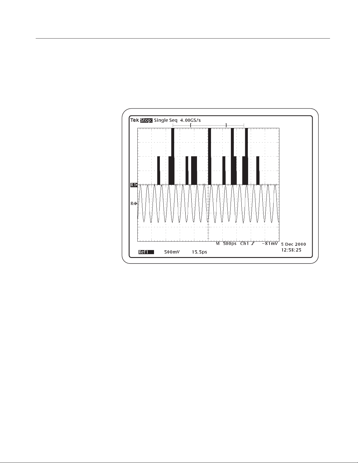
Tutorial
6. Press Vert/Horiz Axis Histogram(side) ➞ Autoset (side) ➞ Done (side).
7. Press the CLEAR MENU front-panel button.
Figure 2–13 shows the Histogram plot.
Figure 2–13: Results as a Histogram plot
8. Press the SHIFT, and then the APPLICATION front-panel menu button to
return to the application.
9. To deselect the Histogram plot, press Off (side) ➞ Done (side).
10. To set up the Time Trend plot format, select Ref2 Plot (side) ➞ On (side).
11. Press the CLEAR MENU front-panel button.
Figure 2–14 shows the Time Trend plot.
TDSJIT1V2 Jitter Analysis Application User Manual
2–33
Page 59
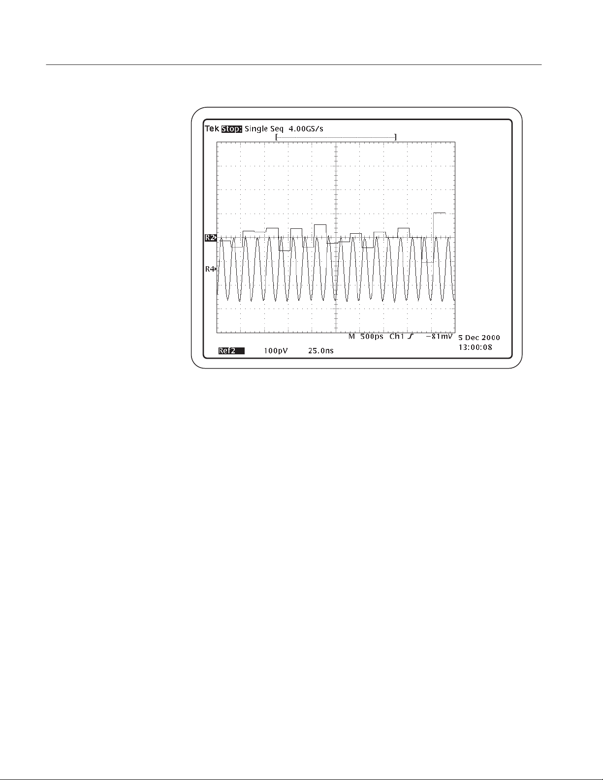
Tutorial
Figure 2–14: Results as a Time Trend plot
12. Press the SHIFT, and then the APPLICATION front-panel menu button to
return to the application.
13. To set up the Spectrum plot format, select –more– 1 of 2 (side) ➞ Spectrum
(side). Figure 2–15 shows the setup for a Spectrum plot.
14. Select State (side) ➞ On (side). As soon as you select On, the Spectrum plot
displays as Math1 in the MORE menu of the oscilloscope.
Figure 2–16 shows the Spectrum plot.
2–34
TDSJIT1V2 Jitter Analysis Application User Manual
Page 60

Tutorial
Figure 2–15: Setup for a Spectrum plot
Figure 2–16: Results as a Spectrum plot
TDSJIT1V2 Jitter Analysis Application User Manual
2–35
Page 61

Tutorial
15. Press the SHIFT, and then the APPLICATION front-panel menu button to
return to the application.
16. To deselect the Time Trend plot, press Done (side) ➞ –more– 2 of 2
(side) ➞ Off (side) ➞ Done (side). This also deselects the Spectrum plot.
17. To set up the Cycle Trend plot format, select Ref3 Plot (side) ➞ On (side).
18. Press the CLEAR MENU front-panel button.
Figure 2–14 shows the Cycle Trend plot.
Figure 2–17: Results as a Cycle Trend plot
19. Press the SHIFT, and then the APPLICATION front-panel menu button to
return to the application.
20. To deselect the Cycle Trend plot, press Off (side) ➞ Done (side).
Taking a Clock Out Time Measurement
In this example, you will learn how to use the application to take Clock Out
Time (clock to output) and Clock Period measurements. To take a Clock Out
Time measurement, you need two waveforms.
2–36
TDSJIT1V2 Jitter Analysis Application User Manual
Page 62
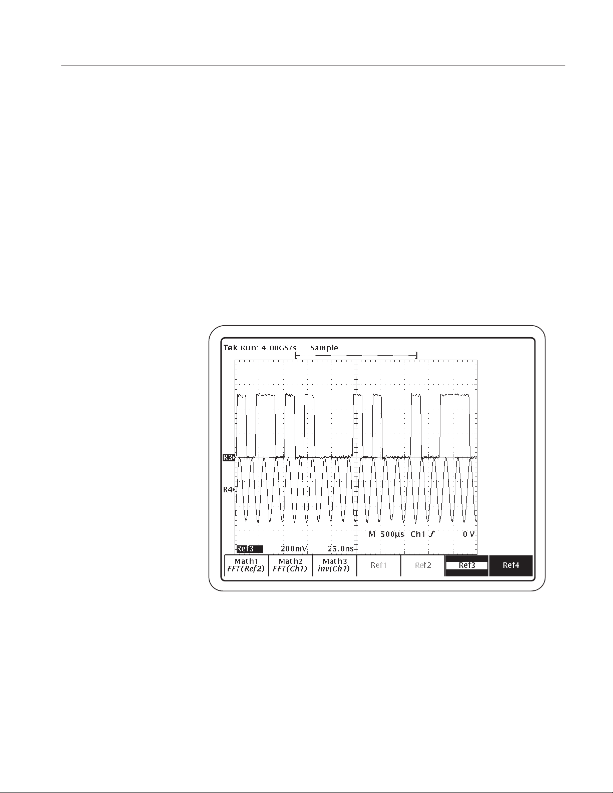
Tutorial
Retain the Main Input setup for Ref1 from the previous lesson. That waveform
will be used in both measurements.
To recall the data waveform to Ref3, follow these steps:
1. Press WAVEFORM ➞ Recall Wfm to Ref (main) ➞ Recall from file (side).
2. Use the general purpose (GP) knob to select hd0: and press SELECT.
3. Use the GP knob to select WFMS and press SELECT.
4. Use the GP knob to select J1V2_DAT.WFM; press To Ref3 active/empty
(side).
5. Press the MORE front-panel button, and then Ref3 (main) to display the
waveform. Use the Vertical Position knob to center the reference waveforms.
Figure 2–18 shows the J1V2_DAT.WFM recalled to Ref3.
Figure 2–18: J1V2_CLK.WFM recalled to Ref3
6. Press the SHIFT, and then the APPLICATION front-panel menu button to
return to the application.
To set up the application to take a Clock-to-Output Time measurement, follow
these steps:
TDSJIT1V2 Jitter Analysis Application User Manual
2–37
Page 63

Tutorial
1. Press Meas Setup (main) ➞ Select Measurement (side) ➞ –more– 1 of 2
(side) ➞ Clock-Data (side) ➞ Clock Out (side), and select On.
2. Press Done (side) two times.
3. Press Select Active Meas (side) and use the GP knob to select Clock-to-Out-
put Time in the list of selected measurements. Figure 2–19 shows the list of
selected measurements.
2–38
Figure 2–19: Selected Measurements list
4. Select Inputs (main) ➞ 2nd (side) ➞ Source (side) ➞ –more– 1 of 4
(side) ➞ –more– 2 of 4 (side) ➞ Ref 3 (side).
5. Press Done (side) two times. Figure 2–20 shows the 2nd Input menu setup.
TDSJIT1V2 Jitter Analysis Application User Manual
Page 64
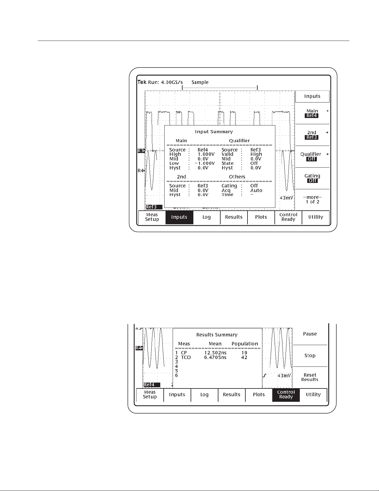
Tutorial
Figure 2–20: 2nd Input menu setup
6. To reset previous results to zero, press Control (main) ➞ Reset Results
(side).
7. To take the measurement, press Control (main) ➞ Start (side).
Wait for the calculations to complete. Figure 2–11 shows the results.
Figure 2–21: Clock Out Time lesson: Results Summary results
TDSJIT1V2 Jitter Analysis Application User Manual
2–39
Page 65

Tutorial
8. Press Results (main) ➞ Result Details (side). Figure 2–22 shows the Results
Details readout.
Figure 2–22: Result Details shows the statistical values for all measurements
Saving the Results to a Data Log File
To save the measurement results to a data log file, follow these steps:
1. Press Log (main) ➞ Log Results (side) and select On.
2. Press Done (side). Figure 2–23 shows the Log Results menu.
NOTE. The RESULTS.CSV file is stored on the hard disk drive by default. It is
faster to save data to a log file on the hard disk drive than to a floppy disk.
2–40
TDSJIT1V2 Jitter Analysis Application User Manual
Page 66
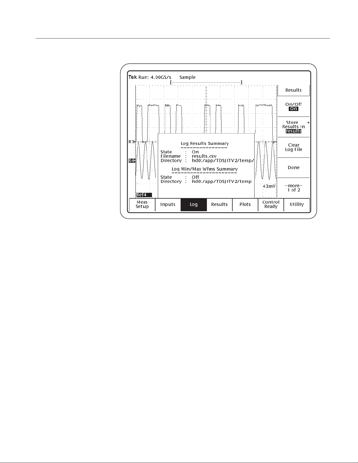
Tutorial
Figure 2–23: Log Results menu
3. To log the results to a .CSV file, press Control (main) ➞ Start (side).
The “comma separated variable” file format (.CSV) is compatible with many
spreadsheet, database, and data analysis programs on a personal computer.
4. After the measurement completes, press Control (main) ➞ Start (side) to log
more data to the RESULTS.CSV file.
5. To copy the RESULTS.CSV file to a floppy disk to view on a personal
computer, follow these steps:
a. Insert a blank, DOS-formatted floppy disk into the floppy disk drive on
the oscilloscope.
b. Press SAVE/RECALL SETUP ➞ File Utilities (main).
c. Use the GP knob to highlight hd0:, and press SELECT.
d. Use the GP knob to highlight APP, and press SELECT.
e. Use the GP knob to highlight TDSJIT1V2, and press SELECT.
f. Use the GP knob to highlight TEMP, and press SELECT.
Figure 2–24 shows the RESULTS.CSV file and the path to it.
TDSJIT1V2 Jitter Analysis Application User Manual
2–41
Page 67
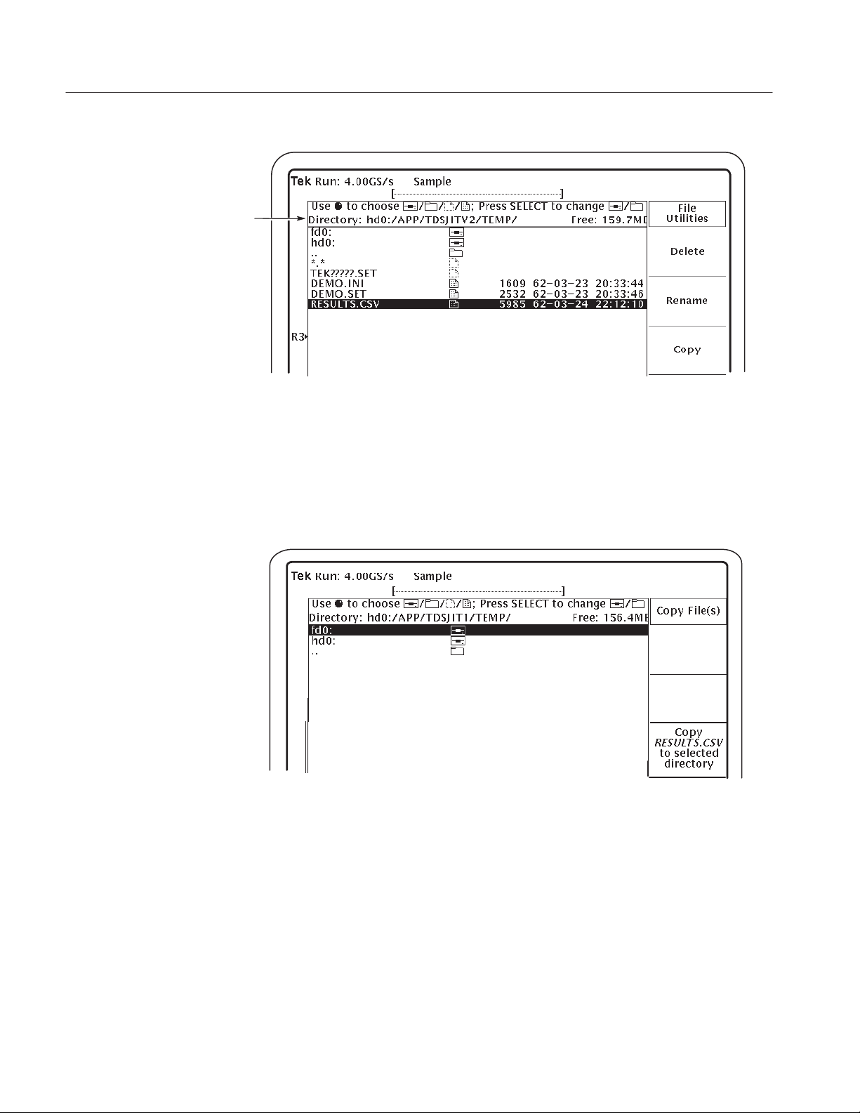
Tutorial
Path to the .CSV file
Figure 2–24: Path to the RESUL TS.CSV file on the hard drive
g. Use the GP knob to highlight RESULTS.CSV, and press Copy (side).
h. Use the GP knob to highlight fd0:, and press Copy RESULTS.CSV to
selected directory (side). Figure 2–25 shows this side menu item.
Figure 2–25: Copying the RESULTS.CSV file to a floppy disk
6. Press the SHIFT, and then the APPLICATION front-panel menu button to
return to the application.
2–42
7. Eject and remove the floppy disk from the floppy disk drive.
TDSJIT1V2 Jitter Analysis Application User Manual
Page 68

Viewing the RESULTS.CSV File (Data Log)
You can import the RESULTS.CSV file to a DOS-based personal computer and
then view the data log file with a spreadsheet, database, or data analysis
program. Figure 2–4 on page 2–15 shows an example of how the RESULTS.CSV file might look in a spreadsheet program on a personal computer.
Stopping the Tutorial
If you need more than one session to complete the tutorial lessons, you can stop
the tutorial and return to it another time. To do so, you will need to save the
application and oscilloscope setups.
To save the setups and stop your session, refer to Saving a Setup on page 2–24
and to Exiting the Application on page 2–25.
Returning to the Tutorial
Tutorial
To return to the tutorial setup, you can start the application and then recall the
saved application and oscilloscope setups from within the application.
To recall the application and oscilloscope setups, refer to Recalling a Setup on
page 2–25.
TDSJIT1V2 Jitter Analysis Application User Manual
2–43
Page 69

Tutorial
2–44
TDSJIT1V2 Jitter Analysis Application User Manual
Page 70

GPIB Program Example
This section contains an example of a GPIB program that can execute the
TDSJIT1V2 application. The application floppy disk contains this program in
the tdsjit1ctrl.c file.
Guidelines
Your GPIB program should comply with the following guidelines:
H Turn off the GPIB response headers with the “HEADER OFF” command;
refer to the programmer information (in online help) for your oscilloscope.
H The application startup must complete before sending additional GPIB
commands to the application (see example).
H The measurements cycle must complete before data is queried (see example).
H The error variable should be checked to ensure that an error has not occurred
because of a measurement command problem.
Program Example
This example shows how a GPIB program might execute the application to do
the following tasks:
H Start the application
H Recall a setup
H Enable the logger
H Take a measurement
H Check for an error
H Exit the application
Refer to Appendix B: GPIB Command Syntax for a complete list of the GPIB
command syntax with the arguments, variables, and variable values.
TDSJIT1V2 Jitter Analysis Application User Manual
2–45
Page 71

GPIB Program Example
/* TDSJITV2
* This is a reference program to illustrate how to communicate to TDSJIT1V2
* using Remote GPIB facilities.
Typical Application does following steps
1. Start up the application
2. Recall a setup
4. Take a measurement
5. Display results or errors
6. Exit the application
For the current program, we will recall ”Default” settings (This has only one active
measurement – Clock Period).
You can save setup files according to your own needs using the application interface.
*/
#ifdef __cplusplus
extern ”C”{
#endif
#include <windows.h>
#include <stdio.h>
#include <stdlib.h>
#include ”decl–32.h”
#ifdef __cplusplus
}
#endif
/* Forward Declarations */
int start_application(int scope);
int exit_application(int scope);
int do_single_test (int scope);
int recall_setup( int scope, char *filename);
void display_results(int scope);
// parameters needed to access the device driver handler
#define BDINDEX 0 // Board Index
#define PRIMARY_ADDR_OF_DMM 1 // Primary address of device
#define NO_SECONDARY_ADDR 0 // Secondary address of device
#define TIMEOUT T10s // Timeout value = 10 seconds
#define EOTMODE 1 // Enable the END message
#define EOSMODE 0 // Disable the EOS mode
2–46
TDSJIT1V2 Jitter Analysis Application User Manual
Page 72

//char ReadBuffer[100]; // Read data buffer
char ErrorMnemonic[21][5] = {”EDVR”, ”ECIC”, ”ENOL”, ”EADR”, ”EARG”,
”ESAC”, ”EABO”, ”ENEB”, ”EDMA”, ””,
”EOIP”, ”ECAP”, ”EFSO”, ””, ”EBUS”,
”ESTB”, ”ESRQ”, ””, ””, ””, ”ETAB”};
/*
* After each GPIB call, the application checks whether the call
* succeeded. If an NI–488.2 call fails, the GPIB driver sets the
* corresponding bit in the global status variable. If the call
* failed, this procedure prints an error message, takes
* the device offline and exits.
*/
void GPIBCleanup(int ud, char* ErrorMsg)
{
printf(”Error : %s\nibsta = 0x%x iberr = %d (%s)\n”,
ErrorMsg, ibsta, iberr, ErrorMnemonic[iberr]);
if (ud != –1)
{
printf(”Cleanup: Taking device offline\n”);
ibonl(ud, 0);
}
exit(0);
}
GPIB Program Example
/* Start Jitter Analysis application */
int start_application( int scope ) {
char write_buffer[100];
char read_buffer[100];
char app_name[] = ”\”TDSJITV2\”\n”;
int status, timer;
/* Start the application */
sprintf(write_buffer, ”%s”, ”Application:activate \”hd0:/TDSJITV2.APP\””);
status = ibwrt(scope, write_buffer, strlen(write_buffer));
if (ibsta & ERR){
GPIBCleanup(scope, ”Unable to start the application”);
return 0;
}
timer = 1;
while (1) {
// Check whether application has started
sprintf(write_buffer, ”%s”, ”Variable:value? \”application\””);
status = ibwrt(scope, write_buffer, strlen(write_buffer));
status = ibrd(scope, read_buffer, sizeof(read_buffer));
read_buffer[ibcnt] = ’\0’;
TDSJIT1V2 Jitter Analysis Application User Manual
2–47
Page 73

GPIB Program Example
if (strcmp(app_name, read_buffer) == 0) {
return 1;
}
timer++;
if (timer > 60) {
return 0;
}
Sleep(1000);
}
return 1;
}
int exit_application(int scope) {
char write_buffer[100];
printf(”Exit Application ...\n”);
sprintf(write_buffer, ”%s”, ”Variable:value \”application\”,\”exit\””);
ibwrt(scope, write_buffer, strlen(write_buffer));
return 1;
}
int recall_setup(int scope, char* filename) {
char write_buffer[100];
char readBuffer[100];
int status;
int timer;
/* set Recall file name */
sprintf(write_buffer, ”%s%s%s”, ”Variable:value \”recallName\”,\””, filename, ”\””);
status = ibwrt(scope, write_buffer, strlen(write_buffer));
if (ibsta & ERR){
GPIBCleanup(scope, ”Unable to communicate with Scope”);
return 0;
}
/* recall setup */
sprintf(write_buffer, ”%s”, ”Variable:value \”setup\”,\”Recall\””);
status = ibwrt(scope, write_buffer, strlen(write_buffer));
if (ibsta & ERR){
GPIBCleanup(scope, ”Unable to communicate with Scope”);
return 0;
}
2–48
TDSJIT1V2 Jitter Analysis Application User Manual
Page 74

/* Check whether recall is complete or not...If recall is complete
variable setup value will change to a blank string */
timer = 1;
while (1) {
if (timer > 60) {
return 0;
}
sprintf(write_buffer, ”%s”, ”Variable:value? \”setup\””);
ibwrt(scope, write_buffer, strlen(write_buffer));
/* read the answer */
ibrd(scope, readBuffer, 99);
if (ibsta & ERR) {
GPIBCleanup(scope, ”Unable to write to device”);
}
readBuffer[ibcnt] = ’\0’;
if (strcmp(readBuffer,”\” \”\n”) == 0) {
return 1;
}
GPIB Program Example
Sleep(1000);
}
return 1;
}
int do_single_test (int scope){
char write_buffer[100];
char read_buffer[100];
int timer;
sprintf(write_buffer, ”%s”, ”Variable:value \”sequencerState\”,\”Sequencing\””);
ibwrt(scope, write_buffer, strlen(write_buffer));
printf(”Executing Test...\n”);
Sleep(100);
// Wait for application to come to Ready State
timer = 1;
while (1) {
if (timer > 90) {
printf(”******Test Time Out ******\n”);
return 0;
}
sprintf(write_buffer, ”%s”, ”Variable:value? \”sequencerState\””);
ibwrt(scope, write_buffer, strlen(write_buffer));
/* read the answer */
TDSJIT1V2 Jitter Analysis Application User Manual
2–49
Page 75

GPIB Program Example
ibrd(scope, read_buffer, 99);
if (ibsta & ERR) {
GPIBCleanup(scope, ”Unable to write to device”);
}
read_buffer[ibcnt] = ’\0’;
if (strcmp(read_buffer,”\”Ready\”\n”) == 0) {
printf(”Test Complete ...\n”);
return 1;
}
Sleep(1000);
}
}
void display_results(int scope) {
char write_buffer[100];
char read_buffer[100];
// Check for errors
sprintf(write_buffer, ”%s”, ”Variable:value? \”error\””);
ibwrt(scope, write_buffer, strlen(write_buffer));
/* read the answer */
ibrd(scope, read_buffer, 99);
if (ibsta & ERR) {
GPIBCleanup(scope, ”Unable to write to device”);
}
read_buffer[ibcnt] = ’\0’;
if (strcmp(read_buffer,”\” \”\n”) != 0) {
printf(”Error has Occured. Error: %s\n”,read_buffer);
return;
}
// If no error, check for results
sprintf(write_buffer, ”%s”, ”Variable:value \”resultFor\”,\”CP\””);
ibwrt(scope, write_buffer, strlen(write_buffer));
Sleep(2000);
printf(”\tClock Period Results\n”);
// ******** Mean
sprintf(write_buffer, ”%s”, ”Variable:value? \”mean\””);
ibwrt(scope, write_buffer, strlen(write_buffer));
/* read the answer */
ibrd(scope, read_buffer, 99);
read_buffer[ibcnt] = ’\0’;
printf(”mean:%s\n”, read_buffer);
2–50
TDSJIT1V2 Jitter Analysis Application User Manual
Page 76

// ******** Max
sprintf(write_buffer, ”%s”, ”Variable:value? \”max\””);
ibwrt(scope, write_buffer, strlen(write_buffer));
ibrd(scope, read_buffer, 99);
read_buffer[ibcnt] = ’\0’;
printf(”max:%s\n”, read_buffer);
// ******** Min
sprintf(write_buffer, ”%s”, ”Variable:value? \”min\””);
ibwrt(scope, write_buffer, strlen(write_buffer));
ibrd(scope, read_buffer, 99);
read_buffer[ibcnt] = ’\0’;
printf(”min:%s\n”, read_buffer);
// ******** PkPk
sprintf(write_buffer, ”%s”, ”Variable:value? \”pkpk\””);
ibwrt(scope, write_buffer, strlen(write_buffer));
ibrd(scope, read_buffer, 99);
read_buffer[ibcnt] = ’\0’;
GPIB Program Example
printf(”pkpk:%s\n”, read_buffer);
// ******** stdDev
sprintf(write_buffer, ”%s”, ”Variable:value? \”stdDev\””);
ibwrt(scope, write_buffer, strlen(write_buffer));
ibrd(scope, read_buffer, 99);
read_buffer[ibcnt] = ’\0’;
printf(”stdDe:v%s\n”, read_buffer);
// ******** population
sprintf(write_buffer, ”%s”, ”Variable:value? \”population\””);
ibwrt(scope, write_buffer, strlen(write_buffer));
/* read the answer */
ibrd(scope, read_buffer, 99);
read_buffer[ibcnt] = ’\0’;
printf(”population:%s\n”, read_buffer);
}
int main(){
int Dev, i;
char write_buffer[100];
int status;
Dev = ibdev (BDINDEX, PRIMARY_ADDR_OF_DMM, NO_SECONDARY_ADDR,
TIMEOUT, EOTMODE, EOSMODE);
TDSJIT1V2 Jitter Analysis Application User Manual
2–51
Page 77

GPIB Program Example
if (ibsta & ERR){
GPIBCleanup(Dev, ”Unable to open device”);
} else {
printf(”My device id – %i”, Dev);
}
sprintf(write_buffer, ”%s”, ”header off”);
status = ibwrt(Dev, write_buffer, strlen(write_buffer));
if (start_application(Dev)) {
printf(”\nApplication started....\n”);
}
recall_setup(Dev, ”Default”);
do_single_test(Dev);
// Print the results
display_results(Dev);
exit_application(Dev);
/* leave the device back elegantly */
printf(”Cleanup: Taking device offline\n”);
ibonl(Dev, 0);
}
2–52
TDSJIT1V2 Jitter Analysis Application User Manual
Page 78

Reference
Page 79
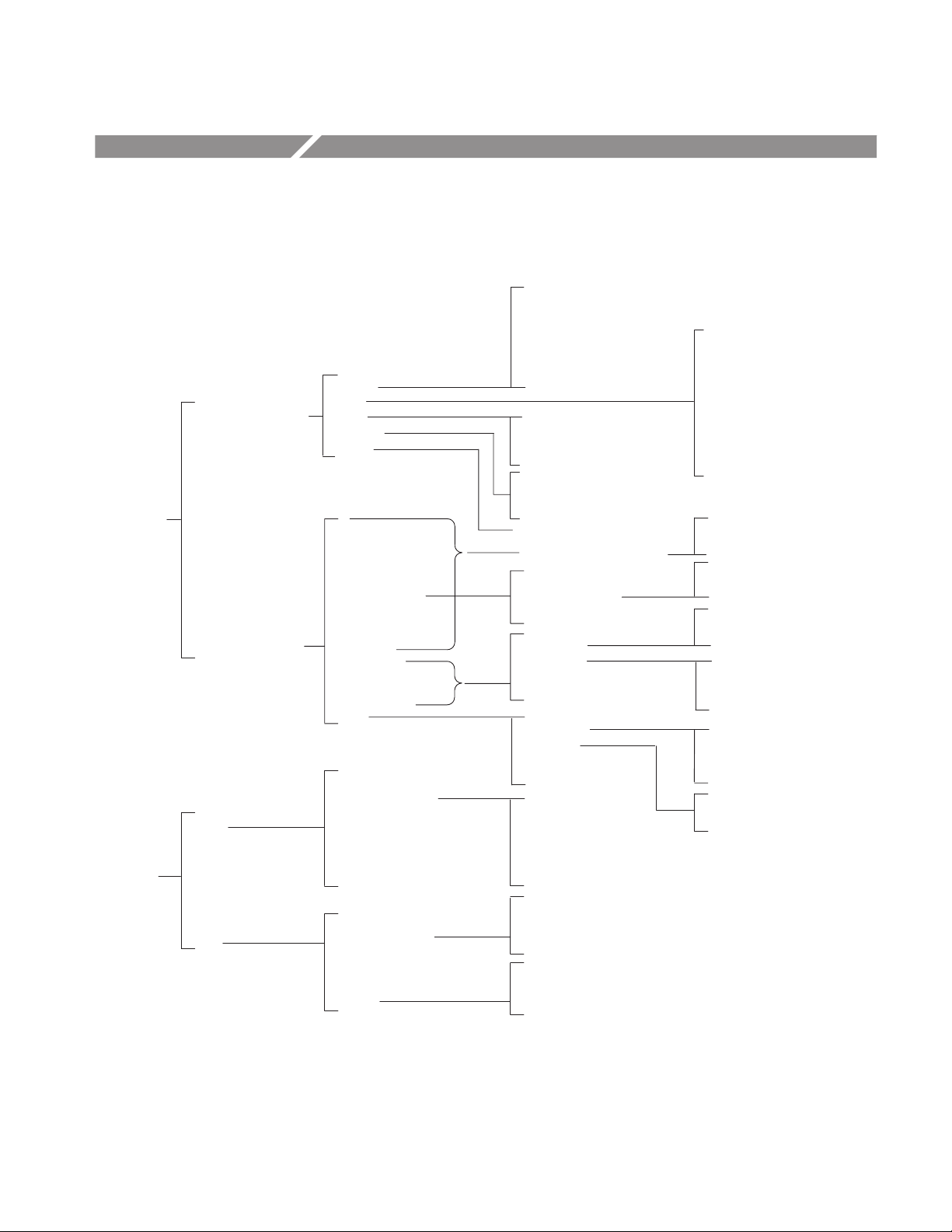
Menu Structure
Select Measurements
Select Active Meas
Clear All Selected
Meas Setup
Configure Selected*
Main
Inputs
Figure 3–1 shows the relationship of the application-specific menus.
Rise Time
Fall Time
General
Clock
Data
Clk-Data
Ch-Ch
Clock Frequency
Clock Period
Cycle-Cycle Period
N - Cycle Period
Positive Duty Cycle
Negative Duty Cycle
Clock TIE
Setup Time
Hold Time
Clock-Out Time
Skew
Source
Autoset Ref Level
Vertical Autoset
Mid Ref
High Ref
Low Ref
Hysteresis
Positive Width
Negative Width
High Time
Low Time
Data Frequency
Data Period
Data TIE
Setup Time
Hold Time
Clock Out Time
Skew
Common Cycle Start Edge
Cycle Span N=
Meas Made Every
Start Meas at Cycle #
Clock Edge
Data Edge
Range Max
Range Min
From Edge
To Edge
Range Max
Range Min
Mid Ref
High Ref
Low Ref
Hysteresis
Perform Autoset
Clock Frequency
Clock Period
Cycle-Cycle Period
N-Cycle Period
Positive Cy-Cy Duty
Negative Cy-Cy Duty
Positive Duty Cycle
Negative Duty Cycle
Clock TIE
Rise
Fall
I
N
Rise
Fall
Rise
Fall
Both
Rise
Fall
Both
Same
Opposite
Source
2nd
* There is no configuration for the Rise Time, Fall Time, Positive Width, Negative Width, High Time, Low Time, Positive Cy - Cy
Duty, Negative Cy - Cy Duty, Data Frequency, Data Period, and Data TIE measurements.
Autoset Ref Level
Vertical Autoset
Mid Ref
Hysteresis
Deskew
Mid Ref
Hysteresis
Perform Autset
Upper Range
Lower Range
Perform Deskew
Figure 3–1: Menu structure
TDSJIT1V2 Jitter Analysis Application User Manual
3–1
Page 80

Menu Structure
Figure 3–2 shows the relationship of the remaining menus.
Inputs
(cont.)
Log
Results
Plots
Control
Utility
Qualifier
Gating
Horizontal Check
Acquisition Timeout
Results
Min/Max Wfms
Summary
Details
Warning
Ref1 Plot
Ref2 Plot
Ref3 Plot
Ref4 Plot
Warning
Mode
Start/Continue
Pause
Stop
Reset Results
Help
Exit
Display Options
Acq Timeout
Timeout
On/Off
Active Meas
Plot Type
Vert/Horiz Axis
Single
Free Run
Single No Acq
First Page
Next Page
Previous Page
Last Page
Quit Help
Dialog Box
Box Position
Box Style
Color Theme
On/Off
Valid When
Source
Mid Ref
Hysteresis
On/Off
Store Results In
Clear Log File
Log Directory
Select Drive
On/Off
Worst Case Directory
Histogram
Cycle Trend
Time Trend (and Spectrum)
(Time Trend)
Vertical Height
Decimation
Length
Spectrum
(Cycle Trend)
Vertical Height
Decimation
State
Destination
Scale
Window
(Histogram)
Autoset
Center
Span
Bin Resolution
Scale
Vertical Height
Refresh
Save/Recall
Figure 3–2: Menu structure (continued)
3–2
Save Name
Save Setup
Recall Name
Recall Setup
TDSJIT1V2 Jitter Analysis Application User Manual
Page 81

Parameters
Measurements Menus
This section describes the TDSJIT1V2 application parameters. You should refer
to the user manual for your oscilloscope for operating details of other controls,
such as front-panel buttons.
Refer to Appendix B: GPIB Command Syntax for a complete list of the GPIB
command syntax with the arguments, variables, and variable values that
correspond to the TDSJIT1V2 parameters.
There are two Meas Setup menus: Select Measurement, and Configure Selected,
and two side menu items: Select Active Meas and Clear All Selected.
The Select Active Meas side menu item displays a list of up to six measurements
activated in the Select Measurements menu. The selected active measurement is
the measurement used as the Configure Selected item.
The Clear All Selected side menu item removes all activated measurements from
the Select Active Meas side menu.
Select Measurements
Menu
Configure Selected Menu
The selections in the Select Meaurements menu by group are as follows:
H General group: Rise Time, Fall Time, Positive Width, Negative Width, High
Time and Low Time
H Clock group: Clock Frequency, Clock Period, Cycle-Cycle Period, N-Cycle
Period, Positive Cy-Cy Duty Cycle, Negative Cy-Cy Duty Cycle, Positive
Duty Cycle, Negative Duty Cycle, Clock TIE
H Data group: Data Frequency, Data Period, and Data TIE
H Clock-Data group: Setup Time, Hold Time, and Clock Out
H Ch-Ch group: Skew
You do not need to configure the following measurements:
H General group (all): Rise Time, Fall Time, Positive Width, Negative Width,
High Time and Low Time
H Clock group: Positive Cy-Cy Duty and Negative Cy-Cy Duty
H Data group (all): Data Frequency, Data Period, and Data TIE
TDSJIT1V2 Jitter Analysis Application User Manual
3–3
Page 82

Parameters
Table 3–1 lists the parameters for the Configure Selected menu and the selections
or range of values available for each.
T able 3–1: Configure Selected menu parameters
Parameter Selections Default setting
Common Cycle Start Edge Rise, Fall Rise
Cycle Span N= 1 to 1,000 in 1 cycle units 6
Meas Made Every 1, N 1
Start Meas at Cycle # 1 to 1,000 in 1 cycle units 1
Common Data Cycle Edge Rise, Fall, Both Rise
Inputs Menus
Range Max –500.0 ms to 500.0 ms in 10 ps units
Range Min –500.0 ms to 500.0 ms in 10 ps units
From Edge Rise, Fall, Both Rise
To Edge Same as From, Opposite as From Same as From
Range Max* –500.0 ms to 500.0 ms in 10 ps units
Range Min* –500.0 ms to 500.0 ms in 10 ps units
* These range values are for the Skew measurement only.
1.0 ms
0 ms
1.0 ms
–1.0 ms
There are four Inputs menus: Main Input, 2nd Input, Qualify Input, and
Acquisition Timeout, and two side menu items: Gating, and Horizontal Check.
Gating makes cursors visible when you select On.
Horizontal Check checks if the Sample Rate is appropriate for the selected
measurements; accurate measurements require at least two samples per edge.
Acquisition Timeout sets the amount of time that the application will wait to
acquire data before it stops and displays an error message
Main Input and 2nd Input
Menus
3–4
Table 3–2 lists the parameters for the Main Input and 2nd Input menus and the
selections or range of values available for each.
TDSJIT1V2 Jitter Analysis Application User Manual
Page 83
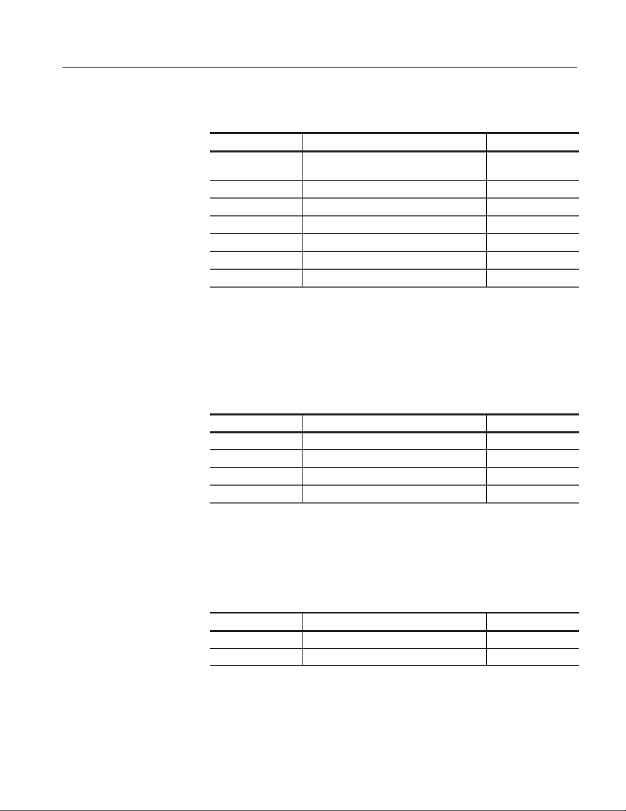
Parameters
T able 3–2: Main Input and 2nd Input menu parameters
Parameter Selections Default setting
Source Ch1, Ch2, Ch3, Ch4, Ref1, Ref2, Ref3, Ref4,
Math1, Math2, Math3*
Autoset Ref Levels Refer to Table 3–3
Vertical Autoset None
Mid Ref –9.99 V to 9.99 V in 0.01 V units 0.00 V
High Ref** –9.99 V to 10.0 V in 0.01 V units 1.00 V
Low Ref** –10.0 V to 9.99 V in 0.01 V units –1.00 V
Hysteresis 0 V to 5.0 V in 0.01 V units 0.00 V
* When deskewing channels, only use Ch1, Ch2, Ch3, or Ch4.
** Only available for the waveform defined in the Main Input menu.
Ch1
Table 3–3 lists the parameters for the Autoset Ref Level menu and the selections
or range of values available for each.
T able 3–3: Autoset Ref Level menu parameters
Parameter Selections Default setting
Mid Ref 1% to 99.0% in 1% units 50%
High Ref** 2% to 99.0% in 1% units 90%
Low Ref* 1% to 98.0% in 1% units 10%
Hysteresis 0% to 50.0% in 1% units 3.0%
* Only available for the waveform defined in the Main Input menu.
Table 3–3 lists the parameters for the Deskew menu and the selections or range
of values available for each.
T able 3–4: Deskew menu parameters
Parameter Selections Default setting
Upper Range –1.0 sec to 1.0 sec in 1 ms units
Lower Range –1.0 sec to 1.0 sec in 1 ms units
1.0 ms
–1.0 ms
TDSJIT1V2 Jitter Analysis Application User Manual
3–5
Page 84

Parameters
NOTE. The Perform Deskew side menu item starts the deskew utility. Refer to
Deskewing the Probes and Channels on page 1–4 for more information.
Qualifier Input Menu
Acquisition Timeout Menu
Table 3–5 lists the parameters for the Qualifier Input menu and the selections or
range of values available for each.
T able 3–5: Qualifier Input menu parameters
Parameter Selections Default setting
On/Off Off, On Off
Valid When Low, High High
Source Ch1, Ch2, Ch3, Ch4, Ref1, Ref2,
Ref3, Ref4, Math1, Math2, Math3
Mid Ref –9.99 V to 9.99 V in 0.01 V units 0.00 V
Hysteresis 0 V to 5.0 V in 0.01 V units 0.00 V
Table 3–6 lists the parameters for the Acquisition Timeout menu and the
selections or range of values available for each.
T able 3–6: Acquisition Timeout menu parameters
Parameter Selections Default setting
Acq Timeout Auto, User Auto
Ref3
Results Menus
Plot Menus
3–6
Timeout 0.1 hrs to 24 hrs in 0.1 hr units* 0.1 hrs*
* When User is selected in the Acq Timeout side menu item.
There are no parameters for the Results Summary, Results Details, or Results
Warning menus.
There are three Plot menus: Histogram, Cycle Trend, and Time Trend. The
Spectrum plot is an FFT of the Time Trend plot and is accessed through the Time
Trend plot menu.
TDSJIT1V2 Jitter Analysis Application User Manual
Page 85

Parameters
Histogram Plot Menu
Table 3–7 lists the parameters for the Histogram Plot menu and the selections or
range of values available for each.
T able 3–7: Histogram Plot menu parameters
Parameter Selections Default setting
Autoset None
Center Refer to Table 3–8
Span Refer to Table 3–8
Bin resolution High, Medium, Low Medium
Scale Linear, Log (logarithmic) Linear
Vertical Height 1.0 V, 2.0 V, 3.0 V, 4.0 V 4.0 V
The parameters for the Horizontal Center and Horizontal Span vary by measurement. Table 3–8 lists the parameter selections and range of values.
T able 3–8: Horizontal Center and Span parameters by measurement
Measurements Parameter Selections Default setting
Rise Time, Fall Time, Positive Width, Negative Width, High Time,
Low Time, Clock Period, and Data Period
Center
Span
10.0 ps to 1.0 s in units of 5 ps
10.0 ps to 1.0 s in units of 5 ps
500 ms
1 s
Cycle-Cycle Period, N-Cycle Period, Positive Cy-Cy Duty, Negative
Cy-Cy Duty , TIE, Data TIE, Setup Time, Hold Time, Clock Out Time,
and Skew
Clock Frequency, Data Frequency Center
Positive Duty , and Negative Duty Center
Cycle Trend Menu
Table 3–7 lists the parameters for the Cycle Trend Plot menu and the selections
Center
Span
Span
Span
or range of values available for each.
T able 3–9: Cycle Trend Plot menu parameters
Parameter Selections Default setting
Vertical Height 1.0 Div, 2.0 Div, 3.0 Div, 4.0 Div 4.0 Div
Decimation Off, On Off
0 s to 500.0 ms in units of 5 ps
10.0 ps to 1.0 s in units of 5 ps
1 Hz to 1 GHz in units of 1 Hz
1 Hz to 1 GHz in units of 1 Hz
0% to 100% in units of 0.1%
0% to 100% in units of 0.1%
500 ms
1 s
500 MHz
1 GHz
50%
100%
TDSJIT1V2 Jitter Analysis Application User Manual
3–7
Page 86

Parameters
T able 3–9: Cycle Trend Plot menu parameters (Cont.)
Parameter Default settingSelections
Length 500, 1000, 2500* 500
* Selections vary and depend on the oscilloscope model and the record length.
Time Trend Menu
Spectrum Menu
Table 3–10 lists the parameters for the Time Trend Plot menu and the selections
or range of values available for each.
T able 3–10: Time Trend Plot menu parameters
Parameter Selections Default setting
Vertical Height 1.0 Div, 2.0 Div, 3.0 Div, 4.0 Div 4.0 Div
Decimation Off, On Off
Length 500, 1000, 2500, 5000, 15000,
30000, 50000*
* Selections vary and depend on the oscilloscope model and the record length.
500
NOTE. The Time Trend plot is limited to a 50,000 point record length; the
Spectrum plot is limited to a 10,000 point record length.
Table 3–11 lists the parameters for the Spectrum Plot menu and the selections or
range of values available for each.
3–8
T able 3–11: Spectrum Plot menu parameters
State On, Off Off
Destination Math1, Math2, Math3 Math1
Scale dB, Linear Linear
Window Data On, Off Off
TDSJIT1V2 Jitter Analysis Application User Manual
Page 87

Log Menus
Parameters
There are two Log menus: Results and Min/Max Wfm.
Results Menu
Min/Max Wfms Menu
Table 3–12 lists the parameters for the Log Results menu and the selections or
range of values available for each.
T able 3–12: Log Results menu parameters
Parameter Selections Default setting
On/Off On, Off Off
Store Results In: RESULTS.CSV, or new file name RESULTS
Clear Log File None
Log Directory hd0:/app/TDSJITV2/temp
Select Drive fd0, hd0 hd0
Table 3–13 lists the parameters for the Log Min/Max Wfms menu and the
selections or range of values available for each.
T able 3–13: Log Min/Max Wfms menu parameters
Parameter Selections Default setting
On/Off On, Off Off
Min/Max Directory hd0:/app/TDSJITV2/temp
Control Menu
Table 3–14 lists the parameters for the Control menu and the selections available.
T able 3–14: Control menu parameters
Parameter Selections Default setting
Mode Single, Free Run, Single No Acq Single
Start (or Continue) None
Pause None
Stop None
Reset Results None
TDSJIT1V2 Jitter Analysis Application User Manual
3–9
Page 88

Parameters
Utility Menus
Table 3–15 lists each utility menu, the parameters, the selections available, and
default settings.
T able 3–15: Utility menus and parameters
Utility menu Parameter Selections Default setting
Help Refer to page 2–1 None
Exit Refer to page 2–25 None
Display Options Dialog Box
Box Position
Box Style
Color Theme
Save/Recall Setup Save Name
Save Setup
Recall Name
Recall Setup
On, Off
Left, Middle, Right
Opaque, Transparent
Based on the TDS oscilloscope
color selections
asetup, or new file name
None
Default, or saved setup file names
None
On
Middle
Opaque
TDS Default
asetup
Default
3–10
TDSJIT1V2 Jitter Analysis Application User Manual
Page 89

Appendices
Page 90

Appendix A: Measurement Algorithms
The TDSJIT1V2 application can take timing measurements from one or two
waveforms. The number of waveforms used by the application depends on the
type of measurement being taken.
Single waveform measurements are: Rise Time, Fall Time, Positive Width,
Negative Width, High Time, Low Time, Clock Period, Clock Frequency,
Cycle-Cycle Period, N-Cycle Period, Positive Cycle-Cycle Duty, Negative
Cycle-Cycle Duty, Positive Duty Cycle, Negative Duty Cycle, Clock TIE, Data
Period, Data Frequency, and Data TIE. Dual waveform measurements are: Setup
Time, Hold Time, Clock-to-Output, and Skew.
Oscilloscope Setup Guidelines
For all measurements, use the following guidelines to set up the oscilloscope:
1. The signal is any channel, reference, or math waveform.
2. The vertical scale for the waveform must be set so that the waveform does
not exceed the vertical range of the oscilloscope.
Test Methodology
3. The sample rate must be set small enough to capture sufficient waveform
detail and avoid aliasing.
4. Longer record lengths increase measurement accuracy. However, you should
be aware of the memory length limitations with Time Trend or Spectrum
plots. For more information, refer to the procedures for viewing the results in
a Time Trend or a Spectrum plot on page 2–19.
The application performs the measurement according to the following steps:
1. Imports the current waveform.
2. Checks that the reference voltage level plus or minus half the hysteresis are
within the 2.5% to 97.5% range of the peak-to-peak waveform values.
3. Checks that there are a minimum number of edges in the waveform to
calculate the measurement as follows:
H Single edge: Rise Time, Fall Time
H One edge pair: Pulse Width, High Time, Low Time
TDSJIT1V2 Jitter Analysis Application User Manual
A–1
Page 91

Appendix A: Measurement Algorithms
H Two cycle-start edges: Frequency, Period, Duty Cycle
H Three cycle-start edges: Cycle-Cycle, TIE
H 2N + 1 cycle-start edges: N-Cycle
H Two edges on each of two waveforms: Skew
4. Performs the measurement.
5. Displays the results as statistics, saves the results as a plot format in a
reference waveform, or saves the results to a data log file.
Edge-Timing Measurements
All timing measurements are based on the time locations of edges within each
acquisition. Edge conditions are defined in the setup menu of each timing
measurement. T
between 1 and the number of edges in the acquisition.
represents the acquisition edge times where n is an index
n
The “i” and “j” represent dissimilar acquisition indices. Dissimilar acquisition
indices occur when the correlation between clock edges and a data transitions are
not one-to-one.
Single Waveform Measurements
The Rise Time and Fall Time algorithms use both the VRefHi and VRefLo
reference voltage levels. Each edge is defined by the slope, voltage reference
level (threshold), and hysteresis.
Rise Time Measurement
The Rise Time measurement is the time difference between when the VRefHi
reference level is crossed and the VRefLo reference level is crossed on the rising
edge of the waveform.
The application calculates this measurement using the following equation:
Rise
T
n
+ T
Hi)
n
Where: T
–T
Lo)
n
Rise
is the rise time.
Hi+
T
is the VRefHi crossing on the rising edge.
A–2
Lo+
is the VRefLo crossing on the rising edge.
T
TDSJIT1V2 Jitter Analysis Application User Manual
Page 92

Appendix A: Measurement Algorithms
Fall Time Measurement
Positive and Negative
Width Measurements
The Fall Time measurement is the time difference between when the VRefLo
reference level is crossed and the VRefHi reference level is crossed on the falling
edge of the waveform.
The application calculates this measurement using the following equation:
Fall
T
n
Where: T
+ T
Lo–
n
–T
Hi–
n
Fall
is the fall time.
Lo–
is the VRefLo crossing on the falling edge.
T
Hi–
is the VRefHi crossing on the falling edge.
T
The Positive Width and the Negative Width measurements are the difference in
time (positive or negative) between the leading edge and trailing edge of a pulse.
The trailing edge is the opposite polarity (direction) of the leading edge.
The application calculates this measurement using the following equation:
)
–
)
–T
n
n
)
–
–T
n
n
W
W
n
n
–
+ T
+ T
High Time Measurement
Where: W+ is the positive pulse width.
–
is the negative pulse width.
W
–
is the VRefMid crossing on the falling edge.
T
+
is the VRefMid crossing on the rising edge.
T
The High Time measurement is the amount of time that a waveform cycle is
above the VRefHi voltage reference level.
The application calculates this measurement using the following equation:
Hi
T
n
+ T
Hi–
n
–T
Hi)
n
Where: THi is the high time.
Hi–
is the VRefHi crossing on the falling edge.
T
Hi+
is the VRefHi crossing on the rising edge.
T
TDSJIT1V2 Jitter Analysis Application User Manual
A–3
Page 93

Appendix A: Measurement Algorithms
Low Time Measurement
Clock Frequency
Measurement
The Low Time measurement is the amount of time that a waveform cycle is
below the VRefLo voltage reference level.
The application calculates this measurement using the following equation:
Low
T
n
Where: T
+ T
Lo)
n
–T
Lo–
n
Low
is the low time.
Lo+
is the VRefLo crossing on the rising edge.
T
Lo–
T
is the VRefLo crossing on the falling edge.
The Clock Frequency measurement calculates the inverse of the clock period for
each cycle.
The application calculates this measurement using the following equation:
Clock
F
n
Where: F
+ 1ńP
Clock
n
Clock
is the clock frequency.
Clock Period
Measurement
Cycle-Cycle Period
Measurement
Clock
P
is the period.
The Clock Period measurement calculates the duration of a cycle as defined by a
start and a stop edge. Edges are defined by slope, threshold, and hysteresis.
The application calculates this measurement using the following equation:
Clock
P
+ T
n
Where: P
n)1
–T
n
Clock
is the clock period.
T is the VRefMid crossing time in the Common Cycle Start Edge
direction.
The Cycle-Cycle Period measurement calculates the difference in period
measurements from one cycle to the next.
The application calculates this measurement using the following equation:
Clock
DPn+ P
n)1
–P
Clock
n
A–4
TDSJIT1V2 Jitter Analysis Application User Manual
Page 94

Appendix A: Measurement Algorithms
Where: DP is the difference between adjacent periods.
Clock
P
is the period.
N-Cycle Period
Measurement
Positive and Negative
Cycle-to-Cycle Duty
Measurements
The N-Cycle Period measurement calculates the difference in period measurements from cycles that are a defined number of cycles apart.
The application calculates this measurement using the following equation:
)
)
)
DNP
–T
n)N
Ǔ–ǒ
ǒ
+
T
n
n)2N
)
n)N
–T
Ǔ
n
T
Where: DNP is the difference between adjacent N-cycle periods.
+
is the VRefMid crossing time in the Common Cycle Start
T
Edge direction.
The Positive Cycle-to-Cycle Duty and Negative Cycle-to-Cycle Duty measurements calculate the ratio of the positive (or negative) portion of the cycle relative
to the period from one cycle to the next.
The application calculates this measurement using the following equation:
DW
DW
)
*
n
+ W
n
+ W
)
)
–W
n
n–1
*
*
–W
n
n–1
Where: DW+ is the positive cycle-to-cycle duty.
DW
W
+
–
Positive and Negative
Duty Cycle Measurements
W
The Positive Duty Cycle and Negative Duty Cycle measurements calculate the
ratio of the positive (or negative) portion of the cycle relative to the period.
The application calculates this measurement using the following equation:
)
D
n
D
–
+ W
n
+ W
–
n
)
n
ńP
ńP
Clock
n
Clock
n
Where: D+ is the positive duty cycle.
TDSJIT1V2 Jitter Analysis Application User Manual
–
is the negative cycle-to-cycle duty.
is the positive pulse width.
is the negative pulse width.
A–5
Page 95

Appendix A: Measurement Algorithms
–
is the negative duty cycle.
D
Clock TIE Measurement
Data Frequency
Measurement
W
+
is the positive pulse width.
–
is the negative pulse width.
W
Clock
is the period.
P
The Clock TIE measurement calculates the difference in time between the
designated edge on a sampled clock waveform to the designated edge on a
calculated clock waveform with a constant frequency (zero jitter).
The application calculates this measurement using the following equation:
Clock
TIE
n
+ Tn–T
Where: TIE
Ȁ
n
Clock
is the clock time interval error.
is the specified clock edge.
T
n
TĂ′n is the calculated ideal clock edge.
The Date Frequency measurement calculates the inverse of the data period for
each cycle.
Data Period Measurement
The application calculates this measurement using the following equation:
Data
F
n
Where: F
+ 1ńP
Data
n
Data
is the data frequency.
P is the period.
The Date Period measurement calculates the duration of a cycle as defined by a
start and a stop edge. Edges are defined by slope, threshold, and hysteresis.
The application calculates this measurement using the following equation:
Data
P
Where: P
+
Data
Data
ǒ
T
n
Ǔ
(
ń
–T
C
n–1
Data
Data
T
is the calculated clock cycle location of T
C
n
)
–C
n
n–1
is the data period.
is the VRefMid crossing time in either direction.
Data
.
n
A–6
TDSJIT1V2 Jitter Analysis Application User Manual
Page 96

Appendix A: Measurement Algorithms
Data TIE Measurement
The Data TIE measurement calculates the difference in time between the
designated edge on a sampled data waveform to the designated edge on a
calculated data waveform with a constant frequency (zero jitter).
The application calculates this measurement using the following equation:
Data
TIE
+ T
n
Where: TIE
Dual Waveform Measurements
Edge conditions are defined for two waveforms. These algorithms use the VRef
values as the reference voltage level. Each edge is defined by the slope, voltage
reference level (threshold), and hysteresis.
Data
n
DataȀ
–T
n
Data
T
direction.
Data
T
Data
is the data time interval error.
is the data edge, the VRefMid crossing time in either
’ is the calculated ideal data edge time.
Setup Time Measurement
Hold Time Measurement
The Setup Time measurement is the elapsed time between the designated edge of
a data waveform and when the clock waveform crosses its own voltage reference
level. The closest data edge to the clock edge that falls within the range limits is
used.
The application calculates this measurement using the following equation:
Setup
T
+ Ti–T
n
Where: T
Data
n
Setup
is the setup time.
T is the Main input (clock) VRefMid
crossing time in the
Main
specified direction.
Data
T
is the 2nd input (data) VRefMid
crossing time in the
2nd
specified direction.
The Hold Time measurement is the elapsed time between when the clock
waveform crosses its own voltage reference level and the designated edge of a
data waveform. The closest data edge to the clock edge that falls within the range
limits is used.
TDSJIT1V2 Jitter Analysis Application User Manual
A–7
Page 97

Appendix A: Measurement Algorithms
The application calculates this measurement using the following equation:
Clock Out Time
Measurement
Hold
T
n
Where: T
+ T
Data
n
–T
i
Hold
is the hold time.
T is the Main input (clock) VRefMid
crossing time in the
Main
specified direction.
Data
T
is the 2nd input (data) VRefMid
crossing time in the
2nd
specified direction.
The Clock Out Time (clock to output) measurement is the elapsed time between
when the clock waveform crosses its own voltage reference level and the
designated edge of a data waveform. The closest data edge to the clock edge that
falls within the range limits is used.
The application calculates this measurement using the following equation:
ClkOut
T
n
Where: T
+ T
do
–T
n
i
ClkOut
is the clock-to-output time.
T is the Main input (clock) VRefMid
crossing time in the
Main
specified direction.
Skew Measurement
do
T
is the 2nd input (data) VRefMid
crossing time in the
2nd
specified direction.
The Skew measurement calculates the difference in time between the designated
edge on a principle waveform to the designated edge on another waveform. The
closest data edge to the clock edge that falls within the range limits is used.
The application calculates this measurement using the following equation:
T
Skew
n
+ Tn–T
S
n
Where: S is the period.
T is the Main input VRefMid
crossing time in the specified
Main
direction.
Ts is the 2nd input VRefMid
crossing time in the specified
2nd
direction.
A–8
TDSJIT1V2 Jitter Analysis Application User Manual
Page 98

Appendix B: GPIB Command Syntax
This appendix describes the GPIB command syntax that you can use in your
GPIB program to do the following tasks:
H Start the TDSJIT1V2 application
H Recognize an active application with GPIB protocol
H Program and read application setup parameters
H Sequence measurements
H Synchronously read measurement results
To use GPIB commands with your oscilloscope, you can use the following
reference materials:
H The tdsjit2ctrl.c file on floppy disk for an example of a GPIB program that
can execute the application
H The GPIB Program Example section for guidelines to use while designing a
GPIB program
H The Parameters Reference section for incremental units and default values of
TDSJIT1V2 parameters
Description. Gives the function of the command, conditions of its use, and its
interactions with other commands.
Syntax. Gives the valid select and query command forms. The required arguments are listed in their proper order.
For example, in the syntax definition
PATH= <Ad><Ars>
the arguments <Ad> and <Ars> are required in the order indicated
Arguments. The arguments to a command are defined along with their range of
values.
Returns. Defines the data returned in response to a command query.
TDSJIT1V2 Jitter Analysis Application User Manual
B–1
Page 99

Appendix B: GPIB Command Syntax
VARIABLE:VALUE TDS COMMAND
Description
VARIABLE:VALUE TDS COMMAND accepts string arguments for a control or
data variable and a value to which to set the argument.
Syntax
VARIABLE:VALUE
VARIABLE:VALUE <variable name>",<variable value>"
the arguments <variable name> and <variable value> are required
in the order indicated.
VARIABLE:VALUE? <variable name>" for query
Arguments and Returns
Table B–1 lists the arguments, their function, and the query returns.
T able B–1: VARIABLE:VALUE TDS COMMAND arguments and queries
Variable name Variable value Function Query form
application {activate “hd0:/TDSJITV2.APP”,
exit}
Sequencer
sequenceMode {Single_NoAcq, FreeRun, Single} Sets the sequencer mode Returns the sequencer mode
Activates the application or terminates the active application
Returns the name of the currently
active application
sequencerState {Ready, Paused, Sequencing} Sets the state of the sequencer:
Sequencing, Ready, Paused
Save/Recall
setup {Default, Recall, Save} Sets the Save/Recall/Default action No query form
recallName Any string from 1 to 8 characters
from A to Z and/or zero to nine
saveName Any string from 1 to 8 characters
from A to Z and/or zero to nine
Logging Results
logAnnotate* Any string from 1 to 20 characters
from A to Z and/or zero to nine
loggerDestination Any string from 1 to 8 characters
from A to Z and/or zero to nine
logDirectory {Default} Sets the directory to the default
logger {Reset} Clears the current statistics log file No query form
Sets the recalled setup file name Returns the saved setup file name
Sets setup file name Returns the setup file name
Provides custom annotation to the
statistics log file
Sets the statistics log file name Returns the statisics log file name
directory
Returns the state of the sequencer
No query form
No query form
B–2
TDSJIT1V2 Jitter Analysis Application User Manual
Page 100

T able B–1: VARIABLE:VALUE TDS COMMAND arguments and queries (Cont.)
Variable name Query formFunctionVariable value
loggerState {On, Off} Sets the state of the statistics log;
when on, the statistics from the
current acquisition are logged
Result Variables
Appendix B: GPIB Command Syntax
Returns the state of the data log
resultFor {CF, CP, TIE, CCP, NCP, PCCD,
NCCD, PDC, NDC, PW, NW,
RISE, FALL, HIGH, LOW, DF, DP,
DTIE, SU, HOLD, TCO, SKEW}
* Custom annotation in the data log file is only available through GPIB execution of the application.
Sets the measurement for which
results are requested
See Table B–2
Table B–2 lists the measurement results queries.
T able B–2: Measurement results queries
Variable name Function
calcFrequency Returns the calculated frequency of the result for the measurement
selected in the resultFor variable
error Returns the error, if any, from the last measurement taken
max Returns the maximum value of the result for the measurement selected
in the resultFor variable
mean Returns the mean value of the result for the measurement selected in
the resultFor variable
min Returns the minimum value of the result for the measurement selected
in the resultFor variable
pkpk Returns the peak-to-peak value of the result for the measurement
population Returns the population for the result for the measurement selected in
positiveMax Returns the positive maximum value for the result of the measurement
positiveMean Returns the positive mean value of the result for the measurement
positivePopulation Returns the positive population for the result for the measurement
negativePopulation Returns the negative population for the result for the measurement
negativeMax Returns the negative maximum value of the result for the measurement
TDSJIT1V2 Jitter Analysis Application User Manual
selected in the resultFor variable
the resultFor variable
selected in the resultFor variable
selected in the resultFor variable
selected in the resultFor variable
selected in the resultFor variable
selected in the resultFor variable
B–3
 Loading...