

Page 1
SOMATOM
Emotion 6/16-slice
configuration
Application Guide
Protocols
Principles
Helpful Hints
Software Version syngo CT 2007E
Page 2

The information presented in this application guide is
for illustration only and is not intended to be relied
upon by the reader for instruction as to the practice of
medicine. Any health care practitioner reading this
information is reminded that they must use their own
learning, training and expertise in dealing with their
individual patients.
This material does not substitute for that duty and is
not intended by Siemens Medical Solutions Inc., to be
used for any purpose in that regard. The drugs and
doses mentioned herein are consistent with the
approval labeling for uses and/or indications of the
drug. The treating physician bears the sole
responsibility for the diagnosis and treatment of
patients, including drugs and doses prescribed in
connection with such use. The Operating Instructions
must always be strictly followed when operating the
MR/CT System. The source for the technical data is the
corresponding data sheets.
The pertaining operating instructions must always be
strictly followed when operating the SOMATOM
Emotion 6/16-slice configuration. The statutory
source for the technical data are the corresponding
data sheets.
We express our sincere gratitude to the many
customers who contributed valuable input.
Special thanks to Christiane Bredenhoeller, Gabriel
Haras, Ute Feuerlein, Jessica Amberg, Thomas Flohr,
Rainer Raupach, Bettina Hinrichsen, Axel Barth,
Kristin Pacheco and the CT-Application Team for their
valuable assistance.
To improve future versions of this application guide,
we would highly appreciate your questions,
suggestions and comments.
Please contact us:
USC-Hotline:
Tel. no. +49-1803-112244
email ct-application.hotline@med.siemens.de
Editors: Wang Jian, Chen Ma Hao
Page 3
Overview
User Documentation 16
Scan and Reconstruction 18
Dose Information 42
Workflow Information 64
Contrast Medium 122
Application Information 136
Head 162
Neck 204
Shoulder 218
Thorax 226
Abdomen 262
Spine 294
Pelvis 314
Upper Extremities 332
Lower Extremities 346
Vascular 360
Specials 416
Radiation Therapy 462
3
Page 4

Overview
Respiratory Gating 484
Children 508
4
Page 5

Overview
5
Page 6

Contents
User Documentation 16
Scan and Reconstruction 18
• Concept of Scan Protocols 18
• Scan Set Up 19
• Feed in/Feed out 19
• Topo Length 20
• Scan Modes 21
- Sequential Scanning 21
- Spiral Scanning 21
-Quick Scan 22
- Dynamic Multiscan 22
- Dynamic Serioscan 22
• UFC detector 23
• Acquisition, Slice Collimation and Slice Width
- SOMATOM Emotion 16-slice configuration
- SOMATOM Emotion 6-slice configuration 26
• Increment 27
• Pitch 27
• Kernels 28
- Head Kernels 32
- Child Head Kernels 32
-Body Kernels 33
- Special Application Kernels 33
• Extended FoV 34
• Auto-FoV 35
• Neuro Modes 37
• Automatic Bone Correction 38
• Positioning 39
• Image Filters 40
24
25
Dose Information 42
• CTDI
and CTDI
W
• ImpactDose 44
• Effective mAs 45
Vol
6
42
Page 7

Contents
• CARE Dose 4D 47
- How does CARE Dose 4D work? 49
- Special Modes of CARE Dose 4D 53
- Scanning with CARE Dose 4D 54
- Adjusting the Image Noise 58
- Activating and Deactivating 61
- Conversion of Old Protocols into Protocols
with CARE Dose 4D 61
- Additional Important Information 63
Workflow Information 64
• WorkStream4D 64
- Recon Jobs 64
- 3D Recon 65
- 1. Sagittal/Coronal Reconstructions 71
- 2. Oblique/Double-oblique Reconstructions
- Non-square Matrix for 3D Recon 76
- Case Examples for 3D Recon and Non-Square
Matrix 77
• Workflow 79
- Patient Position 79
- Auto Reference Lines 79
- Navigation within the Topogram 80
-API Language 81
• e - Logbook 83
- e- Logbook Configuration 83
- e- Logbook subtask card area 87
-e- Logbook Browser 88
- Study Continuation 91
- Reconstruction on the syngo CT Workplace
- Examination Job Status 93
- Auto Load in 3D and Postprocessing Presets
• Scan Protocol Creation 96
- Edit/Save Scan Protocol 96
- Scan Protocol Assistant 98
- Manipulate scan protocols 100
71
92
94
7
Page 8

Contents
- Change parameters 103
- Import scan protocols from SOMATOM
LifeNet/CD 117
Contrast Medium 122
• Contrast Medium 122
- The Basics 122
- IV Injection 125
• Bolus Tracking 126
• Test Bolus using CARE Bolus 128
• Test Bolus 129
- CARE Contrast 130
Application Information 136
• SOMATOM LifeNet 136
- General Information 136
- Key Features 137
- SOMATOM LifeNet offline 138
- SOMATOM LifeNet online 140
• Image Converter 147
• Report Template Configuration 150
• File Browser 151
• Camtasia 155
- Key features 155
- Additional Important Information 159
• Patient Protocol 160
Head 162
• Overview 162
- General Hints 165
- Head Kernels 166
• Scan Protocols 168
- HeadRoutine 168
- HeadNeuro 172
- HeadSeq 174
- InnerEarHR 177
8
Page 9

Contents
- InnerEarHRVol 180
- InnerEar 184
- InnerEarSeq 188
- Sinus 192
- SinusVol 196
- Orbit 198
- Dental 200
Neck 204
• Overview 204
- General Hints 206
- Body Kernels 207
• Scan Protocols 208
- NeckRoutine 208
- NeckThinSlice 212
- NeckVol 214
Shoulder 218
• Overview 218
- General Hints 219
- Body Kernels 219
• Scan Protocols 220
- Shoulder 220
- ShoulderVol 224
Thorax 226
• Overview 226
- General Hints 229
- Body Kernels 231
• Scan Protocols 232
- ThoraxRoutine/
ThoraxRoutine06s 232
- ThoraxCombi/
ThoraxCombi06s 235
- ThoraxVol 240
-ThoraxFast/
9
Page 10

Contents
ThoraxFast06s 244
- ThoraxHR 246
- ThoraxHRSeq 250
- ThoraxECGHRSeq 252
-LungLowDose/
LungLowDose06s 254
-LungCARE/
LungCARE06s 258
Abdomen 262
• Overview 262
- General Hints 264
- Body Kernels 265
• Scan Protocols 266
- AbdomenRoutine/
AbdomenRoutine06s 266
- AbdomenCombi/
AbdomenCombi06s 270
- AbdomenVol 274
- AbdomenFast/
AbdomenFast06s 278
- AbdMultiPhase/
AbdMultiPhase06s 280
- AbdomenSeq 288
- Colonography/
Colonography06s 290
Spine 294
• Overview 294
- General Hints 296
- Body Kernels 297
• Scan Protocols 298
- C-Spine 298
- C-SpineVol 300
- SpineRoutine 302
- SpineThinSlice 304
- SpineVol 305
10
Page 11

Contents
- SpineSeq 308
- Osteo 312
Pelvis 314
• Overview 314
- General Hints 316
- Body Kernels 317
• Scan Protocols 318
- Pelvis 318
- PelvisVol 322
- Hip 324
- HipVol 328
- SI_Joints 330
Upper Extremities 332
• Overview 332
- General Hints 334
- Body Kernels 335
• Scan Protocols 336
- WristHR 336
- ExtrRoutineHR 340
- ExtrCombi 344
Lower Extremities 346
• Overview 346
- General Hints 348
- Body Kernels 349
• Scan Protocols 350
- Knee 350
- Foot 352
- ExtrRoutineHR 354
- ExtrCombi 358
11
Page 12

Contents
Vascular 360
• Overview 360
- General Hints 363
- Head Kernels 364
- Body Kernels 365
• Scan Protocols 366
- HeadAngio/
HeadAngio06s 366
- HeadAngioVol 370
-CarotidAngio/
CarotidAngio06s 372
- CarotidAngioVol 376
- ThorAngioRoutine/
ThorAngioRoutine06s 380
- ThorAngioVol 384
- ThorAngioECG/
ThorAngioECG06s 388
- ThorAngioECGSeq 392
- Embolism/
Embolism06s 394
- BodyAngioRoutine/
BodyAngioRoutine06s 398
- BodyAngioVol 402
-BodyAngioFast/
BodyAngioFast06s 406
- AngioRunOff/
AngioRunOff06s 410
- WholeBodyAngio 414
Specials 416
• Overview 416
- Trauma 416
- Interventional CT 418
- Test Bolus 420
• Trauma Protocols 422
- General Information 422
- Trauma 424
- TraumaVol 425
12
Page 13

Contents
-PolyTrauma/
PolyTrauma06s 426
- HeadTrauma 430
- HeadTraumaSeq 432
- Additional Important Information 434
• Interventional CT - Biopsy 436
- Biopsy 437
- Biopsy Single 438
• Interventional CT - CARE Vision 439
- The Basics 439
- CAREVision 440
- CAREVisionSingle 441
- CAREVisionBone 442
- HandCARE 443
- Additional Important Information 447
• General Information for Biopsy and CARE
Vision 450
- Interventional Toolbar 450
- CAREView 453
- Configuration 456
- Routine Subtask card 458
- Additional Important Information 459
• TestBolus Protocol 460
- TestBolus 460
Radiation Therapy 462
• Radiation Therapy Planning 462
- Benefits 465
• Workflow 468
• Scan Protocols 470
- Overview 470
- RT_Head 472
- RT_Thorax 474
- RT_Breast 476
- RT_Abdomen 478
- RT_Pelvis 480
- Additional Important Information 482
13
Page 14

Contents
Respiratory Gating 484
• Key Features 486
- Respiratory Gating 486
- Respiration Monitoring 486
- Respiration Synchronization 487
• Positioning of the respiratory sensor belt 488
• Scanning Information 490
- Scan Parameters 490
- Temporal Resolution 491
- Technical Principles 491
- Respiratory Triggering 491
- Respiratory gating 492
- Prospective respiratory triggering versus
retrospective respiratory gating 494
- Curve Editor 495
- Synthetic Trigger/Sync 497
• Workflow 498
- Reconstruction and Post processing 498
• Additional important Information 499
• Scan Protocol 500
- RespSeq 500
- Resp 502
- RespModBreathRate 504
- RespLowBreathRate 506
Children 508
• Overview 508
- General Hints 512
- Head Kernels 515
- Body Kernels 516
• Scan Protocols 518
- HeadRoutine 518
- HeadSeq 522
- InnerEarHR 526
- InnerEar 530
- InnerEarSeq 534
- SinusOrbit 538
- NeckRoutine 542
14
Page 15

Contents
- ThoraxRoutine/
ThoraxRoutine06s 546
- ThoraxCombi/
ThoraxCombi06s 550
- ThoraxHRSeq 554
- AbdomenRoutine/
AbdomenRoutine06s 558
- Spine/
SpineRoutine 562
- SpineThinSlice 566
- ExtrRoutineHR 568
- ExtrCombi 570
- HeadAngio/
HeadAngio06s 574
-CarotidAngio/
CarotidAngio06s 578
- BodyAngioRoutine/
BodyAngioRoutine06s 582
-BodyAngioFast/
BodyAngioFast06s 586
- NeonateBody/
NeonateBody06s 587
15
Page 16

User Documentation
For further information about the basic operation,
please refer to the corresponding syngo CT Operator
Manual:
syngo CT Operator Manual Volume 1:
syngo Security Package
Siemens Virus Protection
Basics
SOMATOM LifeNet
syngo Patient Browser
syngo Data Set Conversion
Camtasia
SaveLog
E-Logbook
syngo Viewing
syngo Filming
syngo CT Operator Manual Volume 2:
Preparations
Examination
MPPS
HeartView CT
Respiratory Gating CT
CARE Bolus CT
CARE Vision CT
syngo CT Operator Manual Volume 3:
syngo 3D
syngo Dental CT
syngo Osteo CT
16
Page 17

User Documentation
syngo CT Operator Manual Volume 4:
syngo LungCARE CT
syngo Pulmo CT
syngo Neuro Perfusion CT
syngo Body Perfusion CT
syngo CT Operator Manual Volume 5:
syngo Calcium Scoring
syngo Circulation
syngo Volume Calculation
syngo Dynamic Evaluation
syngo Neuro DSA CT
syngo CT Operator Manual Volume 6:
syngo InSpace 4D CT
syngo Colonography
17
Page 18

Scan and Reconstruction
Concept of Scan Protocols
The scan protocols for adult and children are defined
according to body regions - Head, Neck, Shoulder,
Thorax, Abdomen, Pelvis, Spine, Upper Extremities,
Lower Extremities, Vascular, RT, Specials and
optional Cardiac, PET, SPECT and Private.
The protocols for special applications are defined in the
Application Guide “Clinical Applications” or in the
case of a Heart View examination, in the Application
Guide “Cardiac CT“.
The general concept is as follows: All protocols without
a suffix are standard spiral modes. For example,
“Sinus” means the spiral mode for the sinus.
The suffixes of the protocol name are follows:
“Routine“: for routine studies
“Seq”: for sequence studies
“Fast“: use a higher pitch for fast acquisition
“ThinSlice“: use a thinner slice collimation
“Combi“: use a thinner and a thicker slice collimation
“05s”: use the rotation time of 0.5 seconds
“ECG“: use a ECG-gated or triggered mode
“Neuro“: for neurologicial examinations with a special
mode
“Vol“: use the 3D Recon workflow
“HR“: use a thin slice width for High Resolution studies
A prefix of the protocol name is as follows:
“RT”: for radio therapy studies
The availability of scan protocols depends on the sys-
tem configuration.
“Resp”: for respiratory gated studies
The availability of scan protocols depends on the sys-
tem configuration.
18
Page 19

Scan and Reconstruction
Scan Set Up
Scans can be simply set up by selecting a predefined
examination protocol. To repeat any mode, just click
the chronicle with the right mouse button for repeat.
To delete it, select cut. Each range name in the chronicle can be easily changed before load.
Multiple ranges can be run either automatically with
auto range, which is denoted by a bracket connecting
the two ranges, or separately with a pause in
between.
Feed in/Feed out
The performance of the different buttons (soft buttons, gantry buttons, control box buttons) is standardized as follows:
•in NOT loaded modes
1 mm
•in loaded Biopsy mode:
Feed In/Out = slice width x No. slice positions per scan
2
19
Page 20

Scan and Reconstruction
Topo Length
SOMATOM
Emotion 16
Length [mm] 128, 256, 512, 768, 1024,
1500
Slice width [mm] 4x0.6
Angle Top, Bottom, Lateral
SOMATOM
Emotion 6
Length [mm] 128, 256, 512, 768, 1024,
1500, 1536*, 2000**,
2048***
Slice width [mm] 3x1
Angle AP, PA, Lateral
* only in combination with PET and SPECT, option
** only in combination with SPECT, option
*** only in combination with PET, option
20
Page 21

Scan and Reconstruction
Scan Modes
Sequential Scanning
This is an incremental, slice-by-slice imaging mode in
which there is no table movement during data acquisition. A minimum interscan delay in between each
acquisition is required to move the table to the next
slice position.
Spiral Scanning
Spiral scanning is a continuous volume imaging mode.
The data acquisition and table movements are performed simultaneously for the entire scan duration.
There is no inter-scan delay and a typical range can be
acquired in a single breath hold.
Each acquisition provides a complete volume data set,
from which images with overlapping can be reconstructed at any arbitrary slice position. Unlike the
sequence mode, spiral scanning does not require additional radiation to obtain overlapping slices.
21
Page 22

Scan and Reconstruction
Quick Scan
The data is usually acquired during a full 360° rotation
– this is a Full scan. Data acquisition not using a full
360° rotation is called a “Quick scan”. Quick scans are
employed to reduce motion artifacts and improve the
temporal resolution.
Dynamic Multiscan
Multiple continuous rotations at the same table position are performed for data acquisition. Normally, it is
applied for fast dynamic contrast studies, such as
syngo Neuro Perfusion CT.
Dynamic Serioscan
Dynamic serial scanning mode without table feed.
Dynamic serio can still be used for dynamic evaluation
such as Test Bolus. The image order can be defined on
the Recon subtask card.
22
Page 23
Scan and Reconstruction
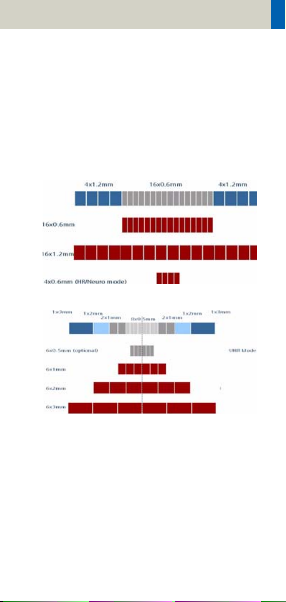
UFC detector
Siemens’ proprietary, high-speed Ultra Fast Ceramic
(UFC) detector enables a virtually simultaneous readout of two projections for each detector element.
The detector configuration with the routine acquisition
of the Emotion 6/16-slice configuration:
SOMATOM Emotion 16-slice configuration:
SOMATOM Emotion 6-slice configuration:
23
Page 24

Scan and Reconstruction
Acquisition, Slice Collimation and Slice Width
Slice collimation is the slice thickness resulting from
the effect of the tube-side collimator and the adaptive
detector array design. In Multislice CT, the Z-coverage
per rotation is given by the product of the number of
active detector slices and the collimation (e.g. 6 x
1.0mm for the SOMATOM Emotion 6-slice configuration or 16 x 0.6mm for the SOMATOM Emotion 16slice configuration ).
Slice width is the FWHM (full width at half maximum)
of the reconstructed image.
With the SOMATOM Emotion 6/16-slice configuration,
you select the slice collimation together with the slice
width desired. The slice width is independent of pitch,
i.e. what you select is always what you get. Actually,
you do not need to care about the algorithm any more;
the software does it for you.
If Metrorecon/Fastrecon is not selected you will routinely get “Real Time” images. The Recon icon on the
chronicle will be labeled with “RT”. After the scan the
Real Time displayed image series has to be reconstructed.
In some cases – this depends also on Scan pitch and
Reconstruction increment – the Recon icon on the
chronicle will be labeled with “RT”. This indicates the
Real Time display of images during scanning. The Real
Time displayed image series has to be reconstructed
after completion of spiral.
The Acq (Acquisition) is displayed on the Examination
task card. The Acquisition is simply "number of slices
acquired per rotation" x "width of one slice".
24
Page 25

Scan and Reconstruction
SOMATOM Emotion 16-slice configuration
Spiral Mode
Collimation/
Acquisition
16 x 0.6 mm 0.75, 1.0, 1.5, 2.0, 3.0, 4.0, 5.0 mm
16 x 1.2 mm 1.5, 2.0, 3.0, 4.0, 5.0, 6.0, 8.0,
HR/Neuro Spiral Mode
Collimation/
Acquisition
4 x 0.6 mm 0.6, 0.75, 1.0, 1.5, 2.0, 3.0, 4.0,
Sequence Mode
Collimation/
Acquisition
4 x 0.6 mm 0.6, 1.2, 2.4 mm
12 x 0.6 mm 0.6, 2.4, 7.2 mm
16 x 0.6 mm 1.2, 2.4, 4.8, 9.6 mm
Slice width
10.0 mm
Slice width
5.0 mm
Slice width
2 x 5 mm 5.0, 10.0 mm
12 x 1.2mm 1.2, 3.6, 4.8 mm
2 x 8 mm 8.0, 16.0 mm
16 x 1.2 mm 2.4, 4.8, 9.6, 19.2 mm
25
Page 26

Scan and Reconstruction
SOMATOM Emotion 6-slice configuration
Spiral Mode
Collimation Slice width
1 mm 1,1.25,2,2.5,3,4,5,6,8,10mm
2 mm 2.5, 3, 4, 5, 6, 8, 10 mm
3 mm 4, 5, 6, 8, 10 mm
Sequence Mode
Collimation Slice width
1 mm 1, 2, 3 mm
2 mm 2, 4, 6, 12 mm
3 mm 3, 6, 9, 18 mm
5 mm 5, 10 mm
HR Spiral Mode
Collimation Slice width
0.5 mm 0.63, 0.75, 1, 1.25, 2, 2.5, 3, 4,
5mm
HR Sequence Mode
Collimation Slice width
1 mm 1 mm
26
Page 27

Scan and Reconstruction
Increment
The increment is the distance between the reconstructed images in Z direction. When the chosen increment is smaller than the slice thickness, the images are
created with an overlap. This technique is useful for
reducing partial volume effect, giving you better detail
of the anatomy and high quality 2D and 3D postprocessing.
The increment can be freely adapted from 0.1 - 10
mm.
Pitch
Pitch = feed per rotation
z-coverage
z-coverage = detector rows x collimated slice width
Feed/Rotation = table movement per rotation
The Pitch Factor can be freely adapted from 0.45 – 2.0,
in Cardio, there is a fixed pitch down to 0.1.
With the SOMATOM Emotion 6/16-slice configuration,
you select the slice collimation together with the slice
width desired.
The slice width is independent of pitch, i.e. what you
select is always what you get. Actually, you do not
need to be concerned about the algorithm any more;
the software does it for you.
Pitch values with a step width of 0.05 can be selected
for all modes.
We recommend to use a Pitch Factor of 0.45 for MPR
reconstructions.
27
Page 28

Scan and Reconstruction
Kernels
There are 4 different types of kernels: “H“ stands for
Head, “B“ stands for Body, “C“ stands for ChildHead and
”S” stands for Special Application, e.g. syngo Osteo CT.
The image sharpness is defined by the numbers – the
higher the number, the sharper the image; the lower
the number, the smoother the image.
Head Kernels:
Kernel description
H10s very smooth
H19s very smooth
H20s smooth
H21s smooth +
H22s smooth FR +
H29s smooth +
H30s medium smooth
H31s medium smooth +
H32s medium smooth FR +
H37s medium smooth (Emotion 16-slice
configuration only)
H39s medium smooth
H40s medium
H41s medium +
H42s medium FR
H45s medium
H47s medium smooth (Emotion 16-slice
configuration only)
H48s medium smooth (Emotion 16-slice
configuration only)
H50s sharp
H60s medium
H70s very sharp
H80s inner ear
H90s inner ear
28
Page 29

Scan and Reconstruction
Body Kernels:
Kernel description
B08s very smooth
B10s very smooth
B19s very smooth
B20s smooth
B29s smooth
B30s medium smooth
B31s medium smooth +
B35s HeartView medium
B39f HeartView medium
B40s medium
B41s medium+
B46s medium
B50s medium sharp
B60s sharp
B65s sharp
B70s very sharp
B75s very sharp (Emotion 16-slice configu-
ration only)
B80s ultra sharp
B90s ultra sharp
Child Head Kernels:
Kernel description
C20s smooth
C30s medium smooth
C60s sharp
29
Page 30

Scan and Reconstruction
Topogram Kernels:
Kernel description
T10s smooth
T20s standard
T21s standard
T80s sharp
T81s sharp
T90s ultra sharp
Special Application:
Kernel description
S30s Shepp-Logan
S80s Shepp-Logan with notch filter
S90s Shepp-Logan without notch filter
U90s specification kernel
30
Page 31

Scan and Reconstruction
PET-Kernel:
Kernel PET
B19s smooth
B29s medium smooth
B39s medium
H19s smooth
H29s medium smooth
H39s medium
SPECT-Kernel:
Kernel SPECT
H08s very smooth
B08s very smooth
31
Page 32

Scan and Reconstruction
Head Kernels
For soft tissue head studies, the standard kernel is
H40s; softer images are obtained with H30s or H20s,
H10s, sharper images with H50s. The kernels H21s,
H31s, H41s yield the same visual sharpness as H20s,
H30s or H40s, respectively. The image appearance,
however, is more acceptable due to a "fine-grained"
noise structure; quite often, the low contrast detectability is improved by using H31s, H41s instead of
H30s, H40s.
In emergency examinations, kernels H22s, H32s, and
H42s can be used because they allow fast reconstruction (FR) and easy patient positioning (50 cm FoV). To
ensure best performance, special online bone correction (PFO) is not used.
High Resolution head studies should be performed
with H50f, H60f (for example, for dental and sinuses).
It is essential to position the area of interest in the center of the scan field.
For a better gray-white brain tissue differentiation use
the H37s, H38s or H47s kernel (Emotion 16-slice configuration only).
Child Head Kernels
For head scans of small children, the kernels C20s,
C30s (for example for soft tissue studies) and C60s (for
example, provided for sinuses) should be chosen
instead of the "adult" head kernels H20s, H30s and
H60s.
32
Page 33

Scan and Reconstruction
Body Kernels
As standard kernels for body tissue studies B30s or
B40s are recommended; softer images are obtained
with B20s or B10s (extremely soft). The kernels B31s or
B41s have about the same visual sharpness as B30s
respectively, B40s, the image appearance, however, is
more acceptable due to a "fine-grained" noise structure; quite often, the low contrast detectability is
improved by using B31s, B41s instead of B30s, B40s.
For higher sharpness, as is required for example, in
patient protocols for cervical spine, shoulder, extremities, thorax, the kernels B50s, B60s, B70s, B80s are
available.
Special Application Kernels
The special kernels are mostly used for "physical" measurements with phantoms, e.g. for adjustment procedures (S80s), for constancy and acceptance tests
(S80s, S90s), or for specification purposes (S90s). For
special patient protocols, S80s and S90s are chosen,
e.g. for osteo (S80s).
Note:
In case of 3D study only, use kernel B10s and at least
50% overlapping for image reconstruction.
Do not use different kernels for body parts other than
what they are designed for.
33
Page 34

Scan and Reconstruction
Extended FoV
SOMATOM Emotion 16/6-slice configuration offers the
extended field of view. The range can be individually
adapted by the user from 50 cm up to 70 cm.
To use this feature you have to select the extended
FoV checkbox on the Recon subtask card. The default
setting is 65 cm, but can be modified.
Extended FoV can be used with each scan protocol.
The extended FoV value should be adapted carefully
to the exact patient size in order to achieve best possible image quality outside the standard scan field.
34
Page 35

Scan and Reconstruction
Auto-FoV
After scanning a topogram the available ranges are displayed in the topo segment. They can be automatically
adapted according to the patient contours. When moving the scan range over the topogram and press the
"ctrl" key simultaneous, the adaptation will be done
automatically. Please make sure, that the whole object
is covered within the default FoV.
In case the FoV is too small, please press the "ctrl" key
and move the scan range over the object once, and it
will be adapted automatically.
The Auto-FoV will also work with the snap function,
when an examination has two or more ranges. The
snap function will also cover the Auto-FoV and therefore you have the possibility to merge different ranges.
To be able to use the snap function, it is necessary to
have the same FoV and the same x and y coordinates
for all available ranges.
Do not use Auto-FoV for asymmetric objects (e.g. only
one arm within the scan field).
35
Page 36

Scan and Reconstruction
Hints
• When positioning the arms along the body, the AutoFoV will also cover the arms.
• When scanning two extremities at the same time,
the Auto-FoV will also cover both extremities.
36
Page 37

Scan and Reconstruction
Neuro Modes
In addition to the standard collimations, the SOMATOM Emotion 16-slice configuration provides a special
mode which is optimized for Neuro applications. Excellent low contrast and detail resolution are achieved.
For spiral scans 4 x 0.6 acquisition mode is provided in
the range of the cerebrum. This approach shows a minimized partial volume effect, i.e. low level of artifacts
in the base of the skull or near vertebral bodies, as
0.6 mm detector rows are used and the narrow collimation reduces scattered radiation.
One scan protocol is predefined for adults:
– HeadNeuro using an acquisition 16 x 0.6 mm in the
base and an acquisition of 4 x 0.6 mm in the cerebrum
We recommend using this special protocol for dedicated Neuro examinations.
For fast standard examinations such as rule out of
hemorrhage or ischemia, the "Routine" protocol should
be used.
37
Page 38

Scan and Reconstruction
Automatic Bone Correction
The head protocols provide significant improvements
regarding image quality for heads. An automatic bone
correction algorithm has been included in the standard
image reconstruction. Using a new iterative technique,
typical artifacts arising from the beam-hardening
effect, for example, Hounsfield bar, are minimized
without additional post-processing. This advanced
algorithm produces excellent images of the posterior
fossa, but also improves head image quality in general.
Bone correction is activated automatically for body
region “Head”. The reconstruction algorithm for “Head”
also employs special adaptive convolution kernels
which help to improve the sharpness-to-noise ratio.
More precisely, anatomic contours are clearly displayed while noise is suppressed at the same time
without causing a blurring of edges.
Head image without
correction.
38
Head image with
corrections.
Page 39

Scan and Reconstruction
Positioning
In order to optimize image quality versus radiation
dose, scans in body regions “Head” and “AngioHead”
are provided within a maximum scan field of 300 mm
with respect to the iso-center. No recon job with a field
of view exceeding those limits will be possible. Therefore, patient positioning has to be performed accurately to ensure a centered location of the skull.
correct positioning wrong positioning
of the head of the head
For trauma examinations of the head we provide two
protocols, to be found in the specials folder:
– HeadTrauma
– HeadTraumaSeq.
The scan protocols enable you to utilize the full 50 cm
FoV, resulting in easier patient positioning for trauma
examinations and to ensure the highest performance,
the dedicated PFO head filter is not used.
39
Page 40

Scan and Reconstruction
Image Filters
If you use kernels, the images are reconstructed again
with the selected kernel value. If you use image filters,
the images are not reconstructed again and the result
is much quicker.
Three different filters are available:
LCE: The Low-contrast enhancement filter enhances
low-contrast detectability. It reduces the image noise.
• Similar to reconstruction with a smoother kernel
• Reduces noise
• Enhances low-contrast detectability
• Adjustable in four steps
• Automatic post-processing
Image taken without
the LCE filter
40
Image taken with the LCE
filter
Page 41

Scan and Reconstruction
"HCE": The High-contrast enhancement (HCE) filter
enhances high-contrast detectability. It increases the
image sharpness, similar to reconstruction with a
sharper kernel.
• Increases sharpness
• Faster than raw-data reconstruction
• Enhances high-contrast detectability
• Automatic post-processing
Image taken without
the HCE filter
"ASA": The Advanced Smoothing Algorithm (ASA)
filter reduces noise in soft tissues while edges with
high contrast are preserved.
• Reduces noise without blurring of edges
• Enhances low-contrast detectability
• Individually adaptable
• Automatic post-processing
Image taken with the
HCE filter
41
Page 42

Dose Information
CTDIW and CTDI
Vol
The average dose in the scan plane is best described by
the CTDIW for the selected scan parameters. The CTDIW
is measured in dedicated plastic phantoms – 16 cm
diameter for head and 32 cm diameter for body (as
defined in IEC 60601 – 2 – 44). For scan modes with zSharp the CTDI100 is calculated using the single number of tomographic sections (not doubled by z-Sharp)
to remain within the terms of IEC 60601-2-44. The zcoverage with and without z-Sharp is the same and so
is the dose. This dose index gives a good estimation of
the average dose applied in the scanned volume, as
long as the patient size is similar to the size of the
respective dose phantoms.
Since the body size can be smaller or larger than
32 cm, the CTDI
value displayed can deviate from the
W
dose in the scanned volume.
The CTDIW definition and measurement are based on
single axial scan modes. For clinical scanning, i.e.scanning of entire volumes in patients, the average dose
will also depend on the table feed between axial scans
or the feed per rotation in spiral scanning. The dose,
expressed as the CTDI
, must therefore be corrected by
W
the pitch factor of the spiral scan or an axial scan series
to describe the average dose in the scanned volume.
For this purpose the IEC defined the term “CTDI
“ in
Vol
September 2002:
CTDI
Pitch factor
=
Vol
CTDI
w
This dose number is displayed on the user interface for
the selected scan parameters.
42
Page 43

Dose Information
Note: Previously the dose display on the user interface
was labeled “CTDIW“. This displayed CTDIW was also corrected for the pitch and was therefore identical to the
current CTDI
The CTDI
tion of the radiation risk associated with CT examination. For this purpose, the concept of the “Effective
Dose“ was introduced by ICRP (International Commission on Radiation Protection). The effective dose is
expressed as a weighted sum of the dose applied not
only to the organs in the scanned range, but also to the
rest of the body. It could be measured in whole body
phantoms (Alderson phantom) or simulated with
Monte Carlo techniques.
The calculation of the effective dose is rather complicated and has to be performed by sophisticated programs. These have to take into account the scan
parameters, the system design of the individual scanner, such as X-ray filtration and gantry geometry, the
scan range, the organs involved in the scanned range
and the organs affected by scattered radiation. For
each organ, the respective dose delivered during the
CT scanning has to be calculated and then multiplied
by its radiation risk factor. Finally, the weighted organ
dose numbers are added up to get the effective dose.
The concept of effective dose allows the comparison of
radiation risk associated with different CT or X-ray
exams, i.e. different exams associated with the same
effective dose would have the same radiation risk for
the patient. It also allows a comparison of the applied
X-ray exposure to the natural background radiation,
for example, 2 – 3 mSv per year in Germany.
.
Vol
value does not provide the entire informa-
w
43
Page 44

Dose Information
ImpactDose
For most of the scan protocols, the effective dose numbers for standard male* and female* are calculated,
and listed the result in the description of each scan protocol.
The calculation was performed using the commercially
available program "ImpactDose" (Wellhoefer Dosimetry).
For pediatric protocols, the ImpactDose calculation
and the correction factors published in "Radiation
Exposure in Computed Tomography"** are used.
These only include conversion factors for ages 8 weeks
and 7 years.
*The Calculation of Dose from External Photon Expo-
sures Using Reference Human Phantoms and Monte
Carlo Methods. M. Zankl et al. GSF report 30/91
**Radiation Exposure in Computed Tomography,
edited by Hans Dieter Nagel, published by COCIR c/o
ZVEI, Stresemannallee 19, D-60596, Frankfurt, Germany.
44
Page 45

Dose Information
Effective mAs
In sequential scanning, the dose (D
) applied to the
seq
patient is the product of the tube current-time (mAs)
CTDIw
per mAs:
w
x mAs
spiral
) is
and the CTDI
D
= D
seq
In spiral scanning, however, the applied dose (D
influenced by the conventional mAs (mA x Rot Time)
and additionally by the pitch factor. For example, if a
Multislice CT scanner is used, the actual dose applied
to the patient in spiral scanning will be decreased
when the pitch factor is greater than 1, and increased
when the pitch factor is less than 1 (for constant mA).
Therefore, the dose in spiral scanning has to be corrected by the pitch factor:
D
spiral
= (D
x mA x Rot Time)
CTDIw
Pitch Factor
To simplify this task, the concept of the “effective“ mAs
was introduced with the SOMATOM Multislice scanners.
The effective mAs takes into account the influence of
pitch on both the image quality and dose:
Effective mAs = mAs
Pitch Factor
To calculate the dose, you simply multiply the CTDI
w
per mAs with the effective mAs of the scan:
D
spiral
= D
x effective mAs
w
CTDI
45
Page 46

Dose Information
For spiral scan protocols, the indicated mAs is the
effective mAs per image. The correlation between tube
current and effective mAs of spiral scans on a Multislice CT scanner is expressed by the following formula:
Effective mAs = mA x RotTime
Pitch Factor
Pitch Factor = Feed per Rotation
nrow x Slice collimation
mA = effective mAs x Pitch Factor
RotTime
where Slice collimation refers to the collimation of one
detector row, and nrow is the number of used detector
rows.
46
Page 47

Dose Information
CARE Dose 4D
CARE Dose 4D is an automated exposure control,
which ensures constant diagnostic image quality over
all body regions at the lowest possible dose.
CARE Dose 4D combines three different adaptation
methods to optimize image quality at the lowest dose
level:
• Automatic adaptation of the tube current to the
patient size
• Automatic adaptation of the tube current to the
attenuation of the patient’s long axis, the so-called zaxis.
• Automatic adaptation of the tube current to the
angular attenuation profile measured online for
each single tube rotation, the so-called angle modulation.
Based on a single a.p. or lateral topogram, CARE Dose
4D determines the adequate mAs level for every section of the patient. Based on these levels, CARE Dose
4D modulates the tube current automatically during
each tube rotation according to the patient’s angular
attenuation profile. Thus, the best distribution of dose
along the patient’s long axis and for every viewing
angle can be achieved.
47
Page 48

Dose Information
Based on a user defined Image Quality Reference
mAs, CARE Dose 4D automatically adapts the (eff.)
mAs to the patient size and attenuation changes
within the scan region. With the setting of the Image
Quality Reference mAs you can adjust image quality
(image noise) to the diagnostic requirements and the
individual preference of the radiologist.
Note: The Image Quality Reference mAs should not
be adjusted to the individual patient size!
48
Page 49

Dose Information
How does CARE Dose 4D work?
CARE Dose 4D combines two types of tube current
modulation:
1) Axial tube current modulation:
Based on a single Topogram (a.p. or lateral) the attenuation profile along the patient’s long axis is measured
in direction of the projection and estimated for the perpendicular direction by a sophisticated algorithm.
Lateral
Attenuation (log)
Scan Range
Example of lateral and a.p. attenuation profile evaluated from an a.p. Topogram.
Based on these attenuation profiles, axial tube current
profiles (lateral and a.p.) and the resulting eff. mAs for
every table position are calculated. The correlation
between attenuation and tube current is defined by an
analytical function which results in an optimum dose
and image noise in every slice of the scan.
49
Page 50

Dose Information
2) Angular tube current modulation:
Based on the above described axial eff. mAs profiles,
the tube current is modulated during each tube rotation. Therefore the angular attenuation profile is measured automatically during the scan and the tube current is modulated accordingly in real time to achieve
an optimum distribution of the X-ray intensity for every
viewing angle.
e
s
rel. tube current
e
s
a
e
e
r
crease
s
c
e
a
e
e
d
r
k d
c
a
e
e
g
d
a
we
r
g
e
n
v
o
a
r
t
s
reference attention
i
o
n
e
g
a
m
i
t
n
a
t
s
n
o
c
o
b
e
se
r
t
s
e
v
a
W
constant dose
s
l
i
m
rel. attenuation
e
s
a
e
r
c
n
i
g
n
o
r
e
s
a
e
r
nc
i
e
g
a
n
i
k
a
e
reference tube current
e
as
e
r
c
Image Quality
Relation between relative attenuation and relative
tube current. The adaptation strength may be
adjusted by user separately for the left branch (slim)
and the right branch (obese) of the curve. This adjustment effects all examinations. The gray lines here
indicates the theoretical limits of the adaptation (constant dose resp. constant image noise). The absolute
(eff.) mAs value is scaled with the Image Reference
mAs value, which may be adjusted in the Scan Card by
the user.
50
Page 51

Dose Information
Scan with constant mA
x-ray dose
Reduced dose level
based on topogram
Real-time angular
dose modulation
slice position
51
Page 52

Dose Information
Principle of automatic tube current adaptation by
CARE Dose 4D for a spiral scan from shoulder to pelvis
(very high table feed for demonstration): High tube
current and strong modulation in shoulder and pelvis,
lower tube current and low modulation in abdomen
and thorax. The dotted lines represent the min. and
max. tube current at the corresponding table position
and result from the attenuation profile of the Topogram.
The mAs value displayed in the user interface and in
the patient protocol is the mean (eff.) mAs value for
the scan range.
The mAs value recorded in the images is the local (eff.)
mAs value.
52
Page 53

Dose Information
Special Modes of CARE Dose 4D
For certain examination protocols CARE Dose 4D uses
modified tube current modulation, to meet specific
conditions, for example:
• for Adult Head protocols the tube current is adapted
to the variation along the patient’s long axis and not
to the angular attenuation profile.
• for Extremities, CARE Vision, syngo Neuro Perfusion
CT, syngo Body Perfusion CT and other special protocols (indicated as CARE Dose), only angular tube current modulation is supported.
• for Osteo and Cardio protocols the mAs setting is
adjusted to the patient size and not modulated during the scan, except if ECG pulsing is switched on.
53
Page 54

Dose Information
Scanning with CARE Dose 4D
If the settings of Image Quality Reference mAs are correctly predefined*, no further adjustment of the tube
current is required to perform a scan.
CARE Dose 4D automatically adapts the tube current to
different patient sizes and anatomic shapes, but it
widely ignores metal implants.
Note: Otherwise the magnification of the topogram
would be distorted which would lead to an underestimation or overestimation of the required eff.
mAs.
For an accurate mAs adaptation to the patient’s size
and body shape with CARE Dose 4D, the patient should
be carefully centered in the scan field.
When using protocols with CARE Dose 4D for body
regions other than those they are designed for, the
image quality should be carefully evaluated.
As CARE Dose 4D determines the (eff.) mAs for every
slice of the topogram, a topogram must be obtained
for use of CARE Dose 4D.
*For Siemens scan protocols of SW version syngo CT
2007E, the settings of CARE Dose 4D are already predefined but may be changed to meet the customer’s
preference of image quality (image noise).
54
Page 55

Dose Information
Outside the topogram range, CARE Dose 4D will continue the scan with the last available topogram information. Without a topogram, CARE Dose 4D cannot be
switched on. Repositioning of the patient on the table
and excessive motion of the patient must be avoided
between the topogram and the scan. If two topograms
of the same projection exist for one scan range, the
last acquired will be used for determining the (eff.)
mAs. If a lateral and a.p. topogram exist for one scan
range, both will be used for determining the (eff.)
mAs.
55
Page 56

Dose Information
After the topogram has been scanned, the (eff.) mAs
value in the Routine tab card displays the mean (eff.)
mAs estimated by CARE Dose 4D based on the topogram*. After the scan has been performed this value is
updated to the mean (eff.) mAs that was applied. The
values may differ slightly due to the online modulation
according to the patient’s angular attenuation profile.
*When tuning the CARE Dose 4D parameter setting to
the individual preference for image quality, we recommend keeping track of this value and comparing
it with the values used without CARE Dose 4D.
56
Page 57

Dose Information
The Quality reference mAs value is displayed on the
Scan tab card. This defines the overall image quality of
the scan protocol currently being used. This value can
be adapted for each protocol according to the user’s
individual requirements of image quality. Here you can
also view the effective mAs value that the system is
going to use for the current scan range.
You can also deselect CARE Dose4D on this tab card.
57
Page 58

Dose Information
Adjusting the Image Noise
The correlation between attenuation and tube current
is defined by the analytical function described above.
This function may be adjusted to adapt the image quality (image noise) according to the diagnostic requirements and the individual preference of the radiologist.
– To adapt the image noise for a scan protocol the
Image Quality Reference mAs value in the Scan tab
card may be adjusted. This value can be adapted for
each protocol according to the user’s individual preferences of image quality, and reflects the mean (eff.)
mAs value that the system will use for a reference
patient with that protocol and the corresponding
body region. The reference patient is defined as a
typical adult, 70 kg to 80 kg or 155 to 180 lbs (for
adult protocols), or as a typical child, 5 years, appr.
20 kg or 45 lbs (for child protocols). Based on that
value, CARE Dose 4D adapts the tube current (or the
mean (eff.) mAs value) to the individual patient size
or body region.
Note: Do not adapt the Image Quality Reference
mAs for an individual patient’s size. Only change
this value if you want to adjust the image quality.
58
Page 59

Dose Information
If you change the quality ref. mAs, a pop-up window is
displayed.
• To change the configuration of CARE Dose 4D,
please open the Examination Configuration dialog
box under Options > Configuration. In the window
that then appears, please double-click the Examina-
tion icon to display the configuration window. The
adaptation strength of CARE Dose 4D may be influenced for slim, obese patients, or body parts of a
patient by changing the CARE Dose 4D settings in
the Patient tab card.
This may be desirable:
– if the automatic dose increase for obese patients (or
patient sections) has to be stronger than the preset
(choose obese: strong increase), resulting in less
image noise and a higher dose for those images.
59
Page 60

Dose Information
– if the automatic dose increase for obese patients (or
patient sections) has to be more moderate than the
preset (choose obese: weak increase), resulting in
more image noise and a lower dose for those
images.
– if the automatic dose decrease for slim patients (or
patient sections) has to be stronger than the preset
(choose slim: strong decrease), resulting in more
image noise and a lower dose for those images.
– if the automatic dose decrease for slim patients (or
patient sections) has to be more moderate than the
preset (choose slim: weak decrease), resulting in
less image noise and a higher dose for those images.
On the Patient tab card you can adjust the image quality (for more information see chapter How does CARE
Dose 4D work).
Note: Changing this adaptation strength effects all
protocols!
60
Page 61

Dose Information
Activating and Deactivating
CARE Dose 4D may be activated or deactivated for the
current scan in the Scan tab card. If CARE Dose 4D is
activated as default, the Image Quality Reference
mAs value is set to the default value of the protocol.
After deactivating CARE Dose 4D, the Image Quality
Reference mAs is dimmed and the (eff.) mAs value
has to be adjusted to the individual patient’s size! If
CARE Dose 4D is switched on again, the Image Quality
Reference mAs is reactivated. Note that the last setting
of the Image Quality Reference mAs or the (eff.) mAs
will be restored when you switch from and back to
CARE Dose 4D usage. The default activation state of
CARE Dose 4D may be set in the Scan Protocol Manager. CARE Dose 4D must be selected (column CARE
Dose type). The corresponding column for activating
CARE Dose 4D is called CARE Dose (4D), with possible
default on or off.
Conversion of Old Protocols into Protocols with CARE Dose 4D
Protocols of SW versions VA70, VA47 and VA45 may be
converted to CARE Dose 4D in the Scan Protocol Manager.
Prior to activating CARE Dose 4D an Image Quality Reference mAs value has to be set in the corresponding
column.
61
Page 62

Dose Information
If you are unsure about the correct Image Quality Reference mAs value, follow this simple procedure:
• Enter the (eff.) mAs value used for that type of protocol without CARE Dose 4D.
• There is a simple way of ascertaining what eff. mAs
CARE Dose 4D will use along the scan range: When
the topogram is complete shrink the scan range to
it's minimum. As you move this small box over the
topogram you can see how the eff. mAs displayed in
the Routine and Scan tab card varies along the
patient's body.
To achieve a certain eff. mAs at a patient's particular
body region you can move the small scan range to
this position and then adjust the Quality reference
mAs so that the displayed eff. mAs value is as
desired. After resizing the scan range to the range
for the examination, carefully observe the displayed
mean eff. mAs. After the subsequent scan is completed inspect the image quality to ensure that the
chosen Quality reference mAs is the right value.
• With that setting perform the first scan and carefully
inspect the image quality. In that first step the dose
may not be lower than without CARE Dose 4D but
will be well adapted to the patient’s attenuation,
resulting in improved image quality.
• Starting from that setting, reduce the Image Quality
Reference mAs step by step to meet the necessary
image quality level.
• Store the scan protocol with the adapted image quality reference mAs.
62
Page 63

Dose Information
Additional Important Information
For ideal dose application it is very important to position the patient in the isocenter of the gantry.
Example for an a.p. topogram:
X-ray tube
Patient
(centered)
Detector
Patient is positioned in the isocenter – optimal dose
and image quality
X-ray tube
Patient
(not centered)
Detector
Patient is positioned too high – increased mAs
X-ray tube
Patient
(not centered)
Detector
Patient is positioned too low – reduced mAs and
increased noise
63
Page 64

Workflow Information
WorkStream4D
Recon Jobs
In the Recon card, you can define up to eight reconstruction jobs for each range with different parameters
either before or after you acquire the data. When you
click on Recon, these jobs are performed automatically
in the background. If you want to add more than
eight recon jobs, simply click the icon for an already
completed recon job in the chronicle with the right
mouse button and select delete recon job. Another
recon job will now become available on the Recon tab
card.
Note: What you delete is just the job from the display,
not the images that have been reconstructed. Once
reconstructed, these completed recon jobs stay in the
browser, until deleted from the local database.
You can also reconstruct images for all scans performed by not selecting any range in the chronicle,
prior to clicking Recon.
Another entry you will find in the right mouse menu is
copy/replace recon parameters. This function is
available for spiral scans only.
The main goal is to support the transfer of volume
parameters between oblique recon jobs of ranges
which cover mainly the same area, e.g., two spiral
scans with/without contrast media.
64
Page 65

Workflow Information
3D Recon
3D Recon allows you to perform oblique and/ or double
oblique reconstructions in any user-defined direction
directly after scanning.
No further post-processing or data loading is needed.
The high-quality SPO (spiral oblique) images are calculated by using the system’s raw data.
Key Features
• Reconstruction of axial, sagittal coronal and oblique/
double oblique images
• 3 planning images in the 3 standard orientations
(coronal, axial, sagittal)
• Image types for planning MPR Thick (10 mm), MIP
Thin (3 mm)
• Field of view and reference image definition possible
in each planning segment
• Asynchronous reconstruction (several reconstruction jobs are possible in the background, axial and
non-axial)
• Workstream 4D performs reconstructions on the
basis of CT raw data
• If the raw data are saved you can start the 3D reconstruction on your syngo CT Workplace.
• It is also possible to perform the reconstruction with
non-square matrix.
65
Page 66

Workflow Information
Workflow Description
WorkStream 4D improves your workflow whenever
non-axial images of a CT scan are required, for example
examinations of the spine.
3D reconstructions are possible:
– spiral scan is needed
– as soon as one scan range is finished and at least one
axial reconstruction job has been performed (RTD or
RTR images).
Select a new recon job and mark Recon Job Type – 3D
on the Recon card. The first recon job that is suitable
for the 3D reconstruction is used as Available plan-
ning volumes.
66
Page 67

Workflow Information
Additional Important Information
Pitch factor for 3D Recon
• For reconstruction of 3D recon jobs the maximum
pitch factor is 1.5.
If the pitch factor is > 1.5 a message window informs
you that this 3D recon job cannot be started and may
be deleted. In this case use the standard 3D task card
with an axial image series for reconstruction.
67
Page 68

Workflow Information
Three planning segments in perpendicular orientations will appear in the upper screen area. You can
choose between MPR Thick (3 mm) and MIP Thin
(10 mm) as the image type for your planning volume
using the relevant buttons.
In each segment you will find a pink rectangle which
represents the boundary of the result images. The
image with the right down marker represents the field
of view (FoV) of the result images (viewing direction).
Right
down
marker
Reference lines
68
Page 69

Workflow Information
The rectangle with the grid represents the reference
image (topogram) which is added to the Topogram
series including the reference lines after reconstruction.
Topographics
indicator
Reference lines
Recon area
69
Page 70

Workflow Information
Preview Image
A preview of the actual FoV is now available.
• After pressing the button Preview Image the actual
FoV to be reconstructed will be displayed.
• Clicking again on the button deactivates the preview
image and displays the whole reference image
again.
• Double clicking into the FoV image activates or deactivates the Preview Image function as well.
If the Preview Image function is active and you move
or rotate the box, or change the recon begin and end
position, the Preview image in the FoV segment will be
updated accordingly.
70
Page 71

Workflow Information
Depending on the desired resultant images, choose
coronal, sagittal or oblique recon axis.
1. Sagittal/Coronal Reconstructions
• Adjust the field of view size to your needs.
• It is only possible to reconstruct images with a
squared matrix.
2. Oblique/Double-oblique Reconstructions
If you want to define the orientation of the result
images independent of the patient’s axis:
• Enable the Free V iew Mode and rotate the reference
lines in the three segments until the desired image
orientation is displayed. The vertical and horizontal
line are always perpendicular to each other. With the
default orientation button you can reset the image
orientation at any time.
• It is only possible to reconstruct images with a
squared matrix.
• Set the field of view to the active segment by clicking
the Set FoV button. The result images will then be
orientated as in the FoV segment. You can adjust the
extension perpendicular to the field of view in the
same way in the other two segments.
71
Page 72

Workflow Information
To define the reference image (topogram) to the active
segment, click on the Set Reference Segment button.
This defines the orientation of the reference image
which will be added to the result images.
Once you have finished the adjustment, start calculation of the result images by clicking on the Recon button. You can start a recon job at any time, independently of other ongoing jobs (asynchronous
reconstruction). After starting the recon job the layout
of the Examination task card changes back to the
standard layout. If "auto recon" is selected, all defined
recon jobs start automatically after scanning.
The progress of reconstruction is displayed by the
slider in the tomo segment.
72
Page 73

Workflow Information
Additional Information
As soon as you define a new recon range, all recon
ranges will be shown in the topo segment. The two
numbers on the right-hand side at the beginning of
each recon range indicate the recon job the range
belongs to. The first number stands for the scan range,
the second number stands for the recon job to which
the range belongs. If no recon job is pending, only the
scan ranges are shown in the topo segment. Only one
number on the right-hand side at the beginning of
each scan range indicates which scan the range
belongs to.
• If the first recon job is saved as an Oblique recon job,
RTD images are displayed after scanning and the
Examination task card is automatically switched to
3D reconstruction
• Patient Browser:
for each double oblique recon job, one series is
added in the Patient Browser.
•If Auto Reference Lines is selected the correspond-
ing reference image is added to the 3D recon series.
• All reconstructions are performed in the background
• Do not use high resolution images
• Do not use extended FoV
• If no entry is selected in the chronicle, all open
reconstructions are automatically reconstructed.
•If Autorecon is selected on the Recon tab card, this
recon job (axial and oblique) will be automatically
reconstructed after scanning.
73
Page 74

Workflow Information
Recon Planning
During planning of a 3D recon range, the image displayed in the FoV segment will be updated to the new
position of the recon start and end position.
The corresponding reference line displayed in both
planning segments is the reference line to the actual
image displayed in the FoV segment.
One click on the start or end position of the recon
range displays either the reference image to the start
position of the recon range or the reference image to
the end position of the recon range in the FoV segment.
Case Examples
Some scan protocols are supplied with predefined
oblique reconstructions. These protocols are
marked with the suffix “VOL”.
•Coronal and sagittal reconstruction of the spine:
– Scan a topogram
– Plan your axial spiral scan range
– Reconstruction of the spiral images (RT images)
– Select Recon job Type sagittal/coronal
– Select the axial image segment
–Press button Set FoV Segment
– Adjust the FoV to your needs
– Define your desired reconstruction parameters
(for example, image type SPO)
– Start reconstruction
– Repeat the reconstruction steps for the other
orientation (sagittal/coronal)
74
Page 75

Workflow Information
• Oblique reconstruction of the sinuses:
– Scan a topogram
– Plan your axial spiral scan range
– Reconstruction of the spiral images
(RT images)
–Select Recon job Type oblique
– Select the sagittal image segment
– Enable Free Mode
– Rotate the reference lines until the best view of the
sinuses is displayed in one of the other segments
– Select this segment and press the Set FoV Seg-
ment button
– Adjust the FoV to your needs
– Define your desired reconstruction parameters
(e.g., image type SPO)
– Start reconstruction
• Oblique reconstruction of the vascular tree:
– Scan a topogram
– Plan your spiral scan range
– Axial reconstruction of the spiral images
(RTD images)
–Select Recon job Type oblique
– Select button MIP Thin as image type for the
planning volume on the toolbar
– Enable Free Mode
– Rotate the reference lines until the best view
of the entire vascular tree is displayed in one of
the other segments
– Select the coronal image segment
– Select this segment and press the Set FoV Seg-
ment button
– Adjust the FoV to your needs
– Define your desired reconstruction parameters
(e.g., Type MIP Thin)
– Start reconstruction
75
Page 76

Workflow Information
Non-square Matrix for 3D Recon
If you perfrom a 3D reconstruction of your spiral scan
you have the possibility to choose between three different FoV matrices: 512 square, 512 non-square, 256
non-square. In some cases it is already saved to the
scan protocol (Spine, CarotidAngio) set up a new scan
protocol or want to modify an existing one you can
save the non-square matrix together with the recon
parameters.
• 512 square: the FoV stays quadratic with a 512x512
matrix size.
• 512 non-square: the FoV can be adjusted as a rectangle to your needs, for example spine reconstruction.
Its max. side ratio is 1:4.
• 256 non-square: the FoV can be adjusted as a rectangle to your needs but with a lower matrix size and a
lower resolution for example RunOff , Cardiac reconstructions. The maximum side ratio is then 1:8.
If you use the non-square matrix and you extend the
side length of your FoV more then the max. ratio then
the shorter side will be stretched to fit into the ratio
again.
You will find the FoV displayed in the image text for the
non-square matrix. It will be displayed like this: FoV X
x FoV Y.
76
Page 77

Workflow Information
Case Examples for 3D Recon and NonSquare Matrix
Some scan protocols are delivered with predefined
oblique and non-square matrix reconstructions.
These protocols are marked with the suffix “VOL”
•Coronal and sagittal reconstruction of the spine:
– Scan a topogram
– Plan your axial spiral scan range
– Reconstruction of the spiral images (RTR/RTD
images)
–Select Recon job Type sagittal/coronal
– Select the axial image segment
–Press button Set FoV Segment
– Select the Matrix size for example, non-square 512
and adjust the FoV to your needs.
– Define your desired reconstruction parameters
(e.g. image type SPO)
– Start reconstruction
– Repeat the reconstruction steps for the other
orientation (sagittal/coronal)
• Oblique reconstruction of the carotid:
– Scan a topogram
– Plan your spiral scan range
– Axial reconstruction of the spiral images
(RTR/RTD images)
–Select Recon job Type oblique
– Select the coronal image segment
– Enable Free Mode
77
Page 78

Workflow Information
– Rotate the reference lines until the best view on
the sinuses is displayed in one of the other segments
– Select this segment and press button Set FoV Seg-
ment button
– Select the Matrix size for example, non-square 512
and adjust the FoV to your needs
– Define your desired reconstruction parameters
(e.g. image type SPO)
– Start reconstruction
• Double-oblique reconstructions of the heart
For detailed information on heart reconstructions
please refer to your "Cardiac CT" Application Guide.
78
Page 79

Workflow Information
Workflow
Patient Position
A default patient position can be linked and stored to
each scan protocol. The SIEMENS default protocols are
already linked to a default patient position.
(Head first - supine)
If a scan protocol is selected and confirmed in the
Patient Model Dialog, the linked patient position
stays active until the user changes it, even if a scan protocol with different patient position is selected.
Auto Reference Lines
The Auto Reference lines settings defined in the
Patient Model Dialog can be linked and saved to each
scan protocol.
If a scan protocol is selected and confirmed in the
Patient Model Dialog, the linked Auto Reference
lines settings stay active until the user changes them,
even if a scan protocol with different Auto Reference
lines settings is selected.
79
Page 80

Workflow Information
Navigation within the Topogram
Navigation within the topogram helps you to plan a
reconstruction range. The minimum conditions for its
use are a scanned range and the availability of RTD
(Real time display) images. After scanning, an orange
line is displayed within the topogram. This line corresponds to the axial image in the tomo segment.
• If you scroll through the axial image stack, the
orange line in the topogram is displayed as a reference line to the currently displayed axial image in the
tomo segment.
• If you change the reconstruction begin or end, the
orange reference line automatically jumps to this
new position and the axial image in the tomo segment will be updated accordingly to the newly
selected position.
• If you move the whole recon box in the topogram,
the orange reference line automatically jumps to this
new position and the axial image in the tomo segment will be updated accordingly to the newly
selected position.
80
Page 81

Workflow Information
API Language
The API language can now be selected directly in the
Patient Model Dialog.
When the API language is selected, only the relevant,
language specific API entries can be selected in the
Scan subtask card. This way it is much easier to select
the correct patient instruction.
81
Page 82

Workflow Information
Before recording a new API text, first define the API language in the API setup dialog under Setup > API/Com-
ment Setup in the main menu.
82
Page 83

Workflow Information
e - Logbook
The goal of e-Logbook is to offer an effective and efficient functionality to process examination information.
The e-Logbook consists of three components:
•The e-Logbook Configuration
•The e-Logbook subtask card area
•The e-Logbook Browser, where all examinations
can be listed for viewing, sorting, searching and
printing
e- Logbook Configuration
You will find the e- Logbook Configuration u nd er
Options >Configuration >e- Logbook Configuration.
The configuration is divided into three tab cards:
•General
• System Entries
• Manual Entries
Under General you can activate and deactivate the e-
Logbook, as default the e-Logbook is activated. If the
e-Logbook is deactivated, no patient information is
recorded.
If you do not want to have the e-Logbook displayed in
the subtask area you can switch it off, even though the
system entries will be recorded.
Additionally you can select a Default printer from a
drop down menu.
83
Page 84

Workflow Information
Over Default Time period you can determine how the
recordings should be listed inside the e-Logbook
Browser:
– Today (which is the default setting)
– This week
– This month
–Yesterday
– Last week
–Last month
Any changes can be saved by selecting "Apply"
84
Page 85

Workflow Information
On the Manual Entries tab card you can configure the
System Entries and Manual Entries, that should be
displayed in the e-Logbook.
System Entries are automatically filled out by the sys-
tem and displayed in the e-Logbook as read-only if
they are configured.
Default settings are:
• Date of Examination
• Patient Name
• Patient ID
•Date of birth
• Scan Protocol Name
•Total mAs
The Continuous Number field is an incremental num-
ber to mark each recorded study within a defined time
range. In addition the Star t No. can be set to ensure for
example an ongoing numbering after a software
update.
85
Page 86

Workflow Information
Furthermore the Continuous Number can be set to:
– Daily
– Monthly
– Yearly
If you set Continuous Number to Daily, the continuous number starts with one each day.
86
Page 87

Workflow Information
Additionally the user can define Manual Entries which
will also be displayed in the e-Logbook. These information can be pre-configured and then selected over a
drop down menu in the e-Logbook.
To configure new entries of the drop down menu for
each Manual Entry, just type the desired information
inside and click on add.
To remove already existing entries, just select the entry
and click on delete.
Additionally you can customize up to five Manual
Entries fields. If you want to rename the customized
entry fields type select Rename.
e- Logbook subtask card area
If you close the current patient examination you will
get an e-Logbook subtask area which shows you all
the information that will be saved in your system. Here
you can edit the manual entries and save these as well
by clicking on "ok".
87
Page 88

Workflow Information
e- Logbook Browser
You will find the e- Logbook Browser in the main
menu under Patient > e- Logbook browser or you can
use F12 key on your keyboard.
You can list the e-Logbook recordings by date. Select
your desired timeframe in the calendar and click List
now.
If you want to list the e-Logbook recordings from
today, click on Tod ay and the recordings will be displayed immediately, no confirmation is needed.
A shortcut to yesterday’s recordings is accessible over
the black arrow on the right side of the Today button.
The system behaves the same if you want to list the
recordings from This Week/Last Week and This
Month/Last Month.
88
Page 89

Workflow Information
Additional to the dates, certain criteria can be selected
to have a more specific search. Search criteria can be
defined for all entries recorded inside the e-Logbook.
For example, the entr y Number of images is recorded.
A search for datasets which have a certain amount of
images can be defined.
Additional conditions can be defined in this case:
– is greater than
– greater or equal
– is less than
– less or equal
– equals
The conditions vary with the selected search criteria.
You will find under the only within drop-down menus
only the System and Manual Entries you have config-
ured before.
The list can be printed:
• Select from the main menu File> Print. The whole
list will be printed at the Default printer, which is
configured under Options> Configuration> e-Log-
book> General.
The list can be exported:
• Select from the main menu File> Export.
•A Save As dialog pops up.
• The list will be automatically exported to H:\Site-
Data\e-Logbook.
• A file name can be given.
The number of columns inside the displayed list
depend on the configurations under Options> Config-
uration> e-Logbook> System/Manual Entries.
89
Page 90

Workflow Information
Hints for the Record List:
1. Calling up Patient Browser
When you double click on any record in the e-Logbook
Browser, the patient data of the Patient Browser will
be opened, if still available and the customer has the
chance to edit the patient information. This change
will also be updated inside the e-Logbook.
2. Updating the Recon List
The e-Logbook is updated automatically when the
examination data has changed within the Patient
Browser with Correct and Rearrange. Patient name,
date of birth, patient ID and study ID will be updated
automatically.
3. Sorting data within the Recon List
You can decide if the data in the Record List should be
listed in ascending or descending order. The default
sorting order is ascending. Just click on the column
head and a small arrow will appear, clicking on it will
change the sorting order.
4. Resizing and reorder the columns
It is possible to reorder the table columns by drag and
drop the column head. For resizing the columns you
just have to move the vertical column lines together.
5. Modify Manual Entries
Make a right mouse click into the cell and modify the
information to your needs. The cell background color
will be changed to green as an indication. Click on the
enabled "Apply" button, then the changes will be
applied to the database and the cell background color
will be white again.
90
Page 91

Workflow Information
Study Continuation
An existing study can be continued at a later time.
To load an existing study:
• Select the desired study in the Patient Browser.
•Select Register from the Patient drop-down menu.
• The patient data is loaded in the Registration dialog
box.
The previous scan protocol is already preselected, but
it is also possible to select any desired scan protocol.
After the patient has been registered, the patient is
loaded into the Examination card.
The ranges already scanned are listed. The following
chronicle entry is shown between the ranges already
scanned and the new ranges: Exam Continue
<Patient Position>.
If you want to continue a contrast media study, the system asks you if the next scan should be continued as a
non-contrast scan instead.
• If you want to continue as a non-contrast scan, the
chronicle entries for the new scan range is indicated
as a non-contrast scan. (No injector symbol is
shown.)
If you continue a study as a contrast study, the chronicle entries of the new scan range are indicated as a
contrast scan. (An injector symbol is shown.)
91
Page 92

Workflow Information
Reconstruction on the syngo CT Work-
place
It is possible to start all reconstructions from your satellite console.
• Raw data has to be available in the local database
• Select the raw data series of the patient in the
Patient Browser and load it into the Recon card
• Plan your recon jobs as usual
92
Page 93

Workflow Information
Examination Job Status
You can get an overview of all recon jobs by clicking on
the recon task symbol in the status bar or selecting
Transfer – Examination Job status in the patient
main menu in the Patient Browser.
The Examination Job Status dialog box will appear
where all recon jobs (completed, queued and in work)
are listed. You can stop, restart and delete each job by
clicking the according button. To give a selected job a
higher priority click urgent.
The column Type shows you which kind of reconstruction is queued.
Two types are displayed:
– Recon
all recon jobs from the Recon card, either on the
syngo Acquisition Workplace or syngo CT Workplace.
– Auto 3D
all 3D reconstructions which you have send via Auto
postprocessing automatically into the 3D Card.
These jobs will be deleted from the job list as soon as
the patient is closed in the 3D card.
93
Page 94

Workflow Information
Auto Load in 3D and Postprocessing Presets
You can activate the Auto load in 3D function on the
Examination task card/Auto Tasking and link it to a
recon job, for example, the 2
slice width in some of the examination protocols. If the
post-processing type is chosen from the pull-down
menu, the reconstructed images will be loaded automatically into the 3D task card on the syngo Acquisi-
tion Workplace with the corresponding post-processing type.
On the 3D task card you can create parallel and radial
ranges for Multi-Planar-Reconstruction (MPR) and Thin
Maximum-Intensity-Projection (MIP Thin), which can
be linked to a special series.
For example, if you always perform sagittal MPRs for a
spine examination, as soon as you load a spine examination into the 3D task card, select the image type
(MPR), orientation, and open the Range Parallel function. Adapt the range settings (image thickness, distance between the images etc.) and click the link button and save your settings. You now have a predefined
post-processing protocol linked to the series description of a spine examination.
nd
recon job with thinner
94
Page 95

Workflow Information
The same can be done for VRT presets. In the main
menu under Type > VRT Definition, you can link VRT
presets with a series description.
Some of the scan protocols, primarily for Angio examinations, are already preset in the protocol with Auto
load in 3D. If you prefer not to have this preset, deselect the Auto load in 3D and save your scan protocol.
Some of the scan protocols are preset in the protocol
with links to a post-processing protocol. If you prefer
not to have this preset, please delete the Range Parallel
preset or overwrite them with your own settings.
95
Page 96

Workflow Information
Scan Protocol Creation
You can modify or create your scan protocols in two
different ways:
• by editing/saving scan protocols
• via scan protocol manager.
Edit/Save Scan Protocol
If you want to modify an existing protocol or create a
new one, for example, you want to have two Abdo-
menRoutine Protocols with different slice widths, we
recommend you do this directly on the Examination
task card.
96
Page 97

Workflow Information
User-specific scan protocols can be saved with the following basic procedure:
• Register a patient, you can choose any patient position in the Patient Model Dialog.
• Select an existing scan protocol in the Patient Model
Dialog.
• Modify the scan protocol, change parameters, add
new ranges etc. to adapt the new protocol to your
requirements.
• Scan your patient as usual.
• Check that all parameters are as you desire.
•Select Edit/Save Scan Protocol in the main menu.
• Select the folder where you want the new protocol to
appear and the scan protocol name in the pop-up
dialog box.
• You can either use the same name to overwrite the
existing scan protocol or enter a new name, which
will create a new protocol name and will not alter
any of the existing protocols already stored.
• If you want to save an "old" protocol again, you may
have to modify the protocol name. The old protocol
(with the old name) must be cancelled explicitly.
97
Page 98

Workflow Information
Additional important information:
• You can save your scan protocol at any time during
the examination.
• It is recommended that you save your own scan protocol under a new name in order to avoid overwriting the default scan protocol.
• Do not use special characters or blanks. Allowed are
all numbers from 0 to 9, all characters from A to Z
and a to z and explicitly the _ (under-score), but no
country-specific characters, for example, à, ê, å, ç, ñ.
• Do not rename scan protocol files at Windows level.
This will lead to inconsistencies.
• You can now save your own scan protocols in any
pre-defined folder. The organ characteristics will
belong to the scan protocol, not to the region.
•In the Patient Model Dialog, the modified scan protocols are marked by a dot in front of the protocol.
Scan Protocol Assistant
If you want to modify special parameters for several
existing scan protocols or you want to modify the
folder structure, we recommend doing this in the
"Scan Protocol Assistant".
You will find the Scan Protocol Assistant under
Options > Configuration in the main menu.
98
Page 99

Workflow Information
Step 1 - What do you want to do?
Four different operation types are possible:
• Manipulate Scan protocols (cut, copy, paste and
delete)
• Change parameters
• Import scan protocols from SOMATOM LifeNet/CD
• Restore protocols to Siemens default
Additional important information
• Each workflow consists of up to five steps, indicated
by the footprints.
• Depending on the workflow step you can list all scan
protocols or all selected scan protocols. The
<Export> button exports the listed scan protocols in
MS Excel recognizable format.
The export file is always created in H:\SiteData\protocols folder. The folder selection cannot be changed.
• The section "Change Parameters" is preselected as
default.
• Depending on the selected workflow in Step 1, the
Scan protocol Assistant leads you through the corresponding steps.
• From Step 3 an <Undo> and <Redo> button are
added. Both buttons only affect the last operation.
• You can navigate through the selected workflow via
the footprints or with the "Back" and "Next" buttons.
With the "Quit" Button you can leave the Scan Proto-
col Assistant at any time without any changes
saved.
99
Page 100

Workflow Information
Manipulate scan protocols
This workflow consists of four steps.
Step 2 - Manipulate scan protocols (cut/copy/paste/
delete)
To be able to modify existing scan protocols you just
have to click with the right mouse button onto the protocol you want to cut, copy or delete, there a menu will
be displayed where you can choose what you want to
do.
Cutting a scan protocol out of one of the folders and
putting it into another one can be done with cut and
then click again on the right mouse button on the
desired folder and you will get the option to paste this
scan protocol there. If you want to leave the scan protocol in the old folder and save it into another one you
just use the copy/paste function. Removing a scan protocol will delete it. Adult and Child protocols are managed separately.
100
 Loading...