

Page 1
Includes
Teacher's Notes
and
Typical
Experiment Results
Instruction Manual and
Experiment Guide for
012-07192A
07/99
the
PASCO scientific
Model SE-9719
DISCOVER DENSITY SET
© 1999 PASCO scientific $7.50
Page 2

Discover Density Set 012–07192A
Page 3

012–07192A Discover Density Set
Table of Contents
Section Page
Copyright, Warranty, and Equipment Return............................................................................... ii
Introduction ................................................................................................................................1
Equipment ................................................................................................................................. 2
Actitivies ................................................................................................................................... 3
The Speed of Sound (Pre-lab) .............................................................................................. 3
Finding an Equation Relating Mass and Volume ................................................................ 5
The Mass of Fluorite Octahedra (Pre-lab) ............................................................................ 7
Finding an Equation Relating Mass and Diameter of Tranparent Plastic Spheres ........... 13
Discovering a Mathematical Equation That Describes Experimental Data (Pre-lab) ....... 1 4
Finding an Equation Relating Mass to Length and Diameter of Black Plastic Cylinders 1 7
Specfications for the Parts ....................................................................................................... 1 9
Teacher’s Notes ...................................................................................................................... 21
Technical Support ....................................................................................................Back Cover
i
Page 4
Discover Density Set 012-07192A
Copyright, Warranty , and Equipment Return
Please—Feel free to duplicate this manual
subject to the copyright restrictions below.
Copyright Notice
The PASCO scientific 012-07192A Discover
Density manual is copyrighted and all rights
reserved. However, permission is granted to nonprofit educational institutions for reproduction of
any part of the manual providing the reproductions
are used only for their laboratories and are not sold
for profit. Reproduction under any other
circumstances, without the written consent of
PASCO scientific, is prohibited.
Limited Warranty
PASCO scientific warrants the product to be free
from defects in materials and workmanship for a
period of one year from the date of shipment to the
customer. PASCO will repair or replace at its
option any part of the product which is deemed to
be defective in material or workmanship. The
warranty does not cover damage to the product
caused by abuse or improper use. Determination of
whether a product failure is the result of a
manufacturing defect or improper use by the
customer shall be made solely by PASCO
scientific. Responsibility for the return of
equipment for warranty repair belongs to the
customer. Equipment must be properly packed to
prevent damage and shipped postage or freight
prepaid. (Damage caused by improper packing of
the equipment for return shipment will not be
covered by the warranty.) Shipping costs for
returning the equipment after repair will be paid by
PASCO scientific.
Credits
Author: Jim Housley
Editor: Sunny Bishop
Equipment Return
Should the product have to be returned to PASCO
scientific for any reason, notify PASCO scientific by
letter, phone, or fax BEFORE returning the product.
Upon notification, the return authorization and
shipping instructions will be promptly issued.
➤ ➤
➤ NOTE: NO EQUIPMENT WILL BE
➤ ➤
ACCEPTED FOR RETURN WITHOUT AN
AUTHORIZATION FROM PASCO.
When returning equipment for repair, the units
must be packed properly. Carriers will not accept
responsibility for damage caused by improper
packing. To be certain the unit will not be
damaged in shipment, observe the following rules:
➀ The packing carton must be strong enough for the
item shipped.
➁ Make certain there are at least two inches of
packing material between any point on the
apparatus and the inside walls of the carton.
➂ Make certain that the packing material cannot shift
in the box or become compressed, allowing the
instrument come in contact with the packing
carton.
Address: PASCO scientific
10101 Foothills Blvd.
Roseville, CA 95747-7100
Phone: (916) 786-3800
FAX: (916) 786-3292
e-mail: techsupp@pasco.com
Web site: www.pasco.com
ii
Page 5

012–07192A Discover Density Set
Introduction
The PASCO SE-9719 Discover Density Set provides materials and activities to
guide students through some basic graphical analysis techniques.
In each case, an example is worked out, with explanations, and then the
student is asked to perform a similar analysis based on the materials in the set.
In the first analysis, students discover the concept as a mathematical constant
relating measurements of a particular substance.
Then they are asked to discover experimentally an equation that predicts the
mass of spheres of unknown, but constant, composition, based on their
diameter.
Finally, they are lead to develop an equation in three variables that predicts the
mass of cylinders of unknown, but constant, composition, based on
measurements of their diameter and length.
The only mathematical formula students are expected to know is that for slope.
If they recall special volume formulas for spheres and cylinders, they are asked
not to use this information in the development of their equations. After
graphical analysis yields the desired equations, students can use volume
formulas and tabulated density data to verify the correctness of the equations
they have discovered experimentally.
Other Uses
Because the items in the set are machined to close tolerances, and dimensions
and masses are given in the teacher’s guide, the set may be used for other
purposes, such as a traditional density set, or as items to test students’ ability to
make accurate measurements, etc.
1
Page 6
Discover Density Set 012–07192A
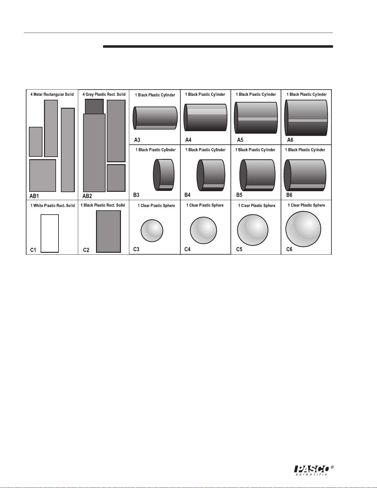
Equipment
Included:
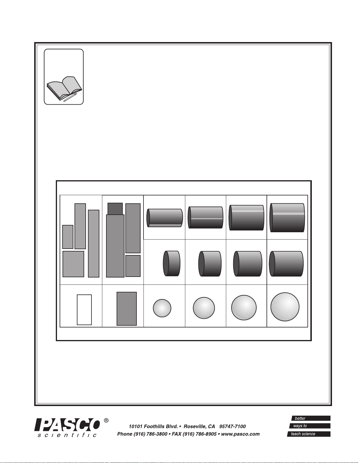
• PASCO SE-9719 Discover Density Set
Figure 1
Contents of the SE-9719 Discover Density Set
2
Page 7
012–07192A Discover Density Set
Activities
The Speed
of Sound
(pre-lab)
Introduction
This sample problem presents you with experimental data, and then leads you
through a process to obtain an equation that relates the data. A similar problem
based on the materials in this set is left for you to do, based on the same
process. The method is then extended to more complex situations.
A lightning bolt struck the earth, and upon seeing it, a number of observers
started timing, using stopwatches. The observers each stopped their watches
when they heard the thunder. The times recorded, and the distances of the
observers from the point the lightning struck are recorded in the table. The
variables have arbitrarily been labeled x and y:
x y
time distance
(s) (km)
3.7 1.2
5.2 1.8
8.3 2.8
12.1 4.1
14.9 5.1
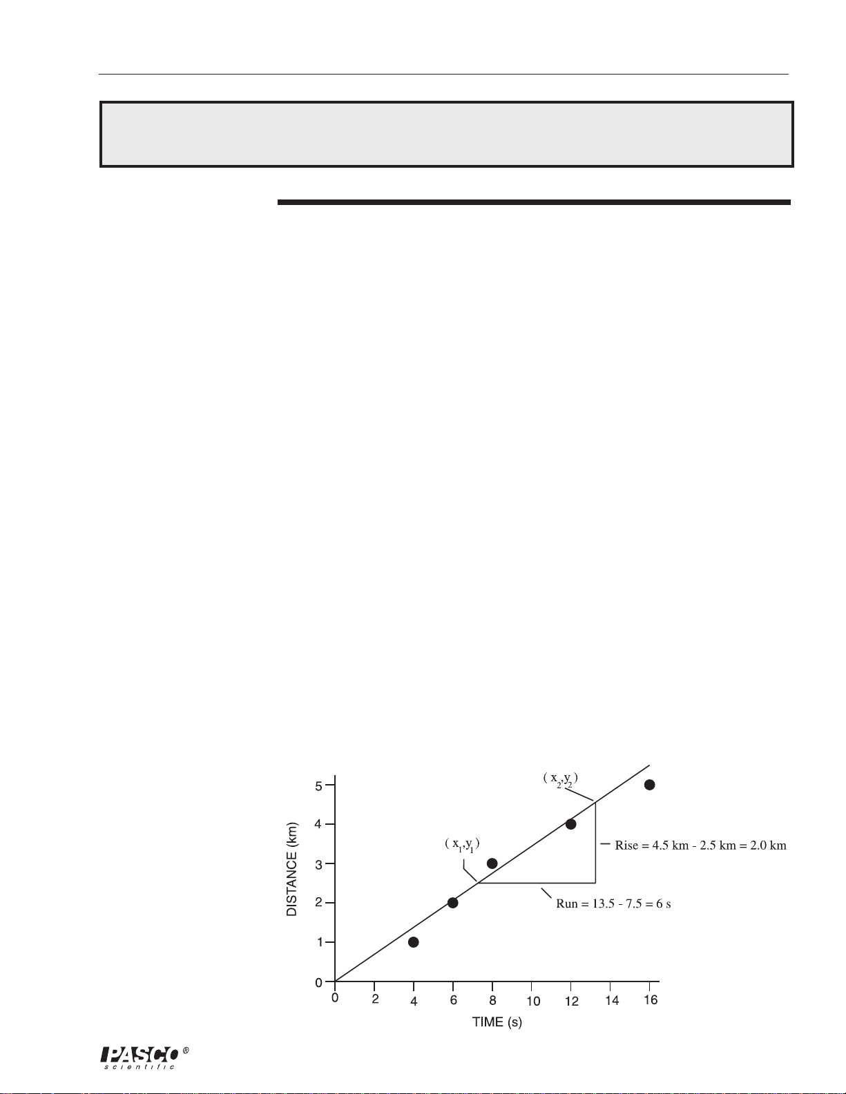
Figure 2
Graph of Speed of
Sound data
When this data is graphed, a straight line can be drawn that closely
approximates the pattern of the data. We may assume that there are errors in
the data caused by factors such as random differences in human reaction time
in actuating the stopwatches, and inaccuracies of an unpredictable nature in
measuring the distances. Such errors may be the reason that the points do not
all fall exactly on the line.
3
Page 8

Discover Density Set 012–07192A
In algebra, the formula for a graph such as above is often given by:
y = m x + b,
where y is the variable on the vertical axis,
x is the variable on the horizontal axis,
b is the point on the vertical axis where the line intersects, and
m is the slope of the line.
The slope is found by marking two points on the line, and dividing the
difference in y-coordinates (called the rise) by the difference in x-coordinates
(the run).
Since all parts of a straight line have the same slope, the slope is a constant for
this experiment.
For this data, b is zero, and m is 2.0 km / 6.0 s = 0.33 km/s
Notice that dimensional units are part of the rise and of the run. The slope is
found in this case by dividing a distance by a time. You should recognize this
as the formula for speed.
The algebra equation y = m x + b may be translated into an equation
appropriate to this situation by replacing the algebra symbols with the variables
in the problem.
Thus, distance = speed * time, a very familiar equation!
The speed in this case is the speed of sound, and is in agreement with
published data, considering uncertainty.
This example is intended as a simple illustration of how numerical data from
an experiment is transformed from a table to a graph to a meaningful equation.
4
Page 9

012–07192A Discover Density Set
Finding an
Equation
Relating
Mass and
Volume
Introduction
In this activity you are given four rectangular solid metal pieces, and four
similar plastic pieces. You are asked to take data, organize it, graph it, and
create equations relating the mass and volume of each of the two kinds of
material. A minimum of instructions are given. You should study and follow
the example titled “The Speed of Sound” which preceded this task.
Materials required
The materials needed are in compartments AB1, AB2, C1, and C2.
Procedure
1. Create a table to record the length, width, and height, volume, and mass of
the four metal pieces from compartment AB1, and a similar table for the
four gray plastic pieces from compartment AB2.
2. Record the length, width, and height in centimeters. If you are using a
metric ruler, estimate to the nearest 0.01 cm when finding these
dimensions. Use the rules regarding significant figures or other
appropriate methods of expressing uncertainty.
3. Consider the volume to be the independent variable, and the mass to be
the dependent variable when graphing the data. Prepare a graph that
shows the data for all eight objects, labeling your data points for the metal
pieces with circles, and the data points for the gray plastic pieces with
squares.
4. Draw a best-fit line for the data from the metal pieces, and another for the
data from the grey plastic pieces. If straight lines passing through the
origin do not represent the data well, recheck your measurements and
calculations for any data points that do not fit the pattern.
5. Calculate the slope of each line, and include dimensional units as part of
your calculations. Show your calculations, and use significant figures or
another appropriate expression of uncertainty.
6. Although each item had its own mass and volume, the slope of the line for
the metal pieces is constant. The metal pieces are all aluminum, and the
slope is termed the density of aluminum. Find a published value for the
density of aluminum, and compare to your value. Does your value agree
within the limits of uncertainty?
7. The gray plastic is polyvinyl chloride, or PVC. Its published density is
1.36 to 1.40 g/cm
uncertainty?
3
. Does your value agree within the limits of
5
Page 10

Discover Density Set 012–07192A
8. Write equations for each of the two lines obtained. Use meaningful
symbols, such as “m” and “v”. Include dimensional units in the
constant.
9. Find the mass, volume, and density of the transparent rectangular solid
and the black rectangular solid from compartments C1 and C2. Plot
them on the same graph as the aluminum and PVC. Ignoring the color,
can you say with confidence that they are or are not the same type of
plastic as PVC, or as each other?
6
Page 11

012–07192A Discover Density Set
The Mass
of Fluorite
Octahedra
(Pre-lab)
Introduction
Developing a mathematical equation from a set of experimental data is an
extremely useful skill. The examples that follow show a method that will
work for a great many physics phenomena. Then you will be asked to apply
the method to data in a lab situation.
The mineral fluorite is often found in geometric shapes having eight faces
which are equilateral triangles. This example addresses the problem of
finding an equation that allows one to calculate the mass of such a fluorite
specimen from a measurement of one of the edges.
Experimental Data
Some data were obtained from direct measurement of five fluorite specimens:
xy
edge mass
(cm) (g)
0.8 0.8
1.3 3.3
2.0 12.0
2.7 29.5
3.7 75.9
Graphing this data in the ordinary manner is a good first step. The results
suggest an equation such as y = x
multiplier would likely be present, resulting in an equation such as y =
2
0.57x
, or y = 3.9x2. Finally, if the exponent were a number such as (3/2) or
2.716, the same basic shape of graph would still result. Quite often in
physics, and particularly in simple situations such as this, the exponent will
be either a small integer, or a ratio of two small integers.
2
, or y = x3. Of course, a constant
Data Analysis
All of the equations above are of the form y = c xk, where c and k are two
different constants. Many equations in physics, although certainly not all, are
of this form.
If an initial graph or other reasoning make it reasonable to assume an
equation of the form of the form y = c x
values of c and k. Several methods exist for doing this. The first might be
called “guess and test.”
k
, the next task is to determine the
7
Page 12

Discover Density Set 012–07192A
We might guess, for the fluorite example, that the exponent is 2, so y = c x2.
This could be expressed in words as “y is proportional to x
2
.” Making a
new table results in the following: (A computer spreadsheet program is an
efficient way of creating such tables.)
2
x
2
edge
2
(cm
) (g)
y
mass
0.6 0.8
1.7 3.3
4.0 12.0
7.3 29.5
13.7 75.9
A graph of the above data does not result in a straight-line, as would have
been the case if y had been proportional to x
2
. See Figure 3.
Figure 3
Graph of x2 vs mass
8
Page 13

012–07192A Discover Density Set
The corresponding graph from table of x3 and y values is straight, and thus
shows that y is proportional to x
3
. See Figure 4.
3
x
3
edge
3
(cm
) (g)
y
mass
0.5 0.8
2.2 3.3
8.0 12.0
19.7 29.5
50.7 75.9
Figure 4
Graph of x3 vs mass
The analysis has established that y = c x
simply the slope of the graph. Picking two points (x
3
. The constant of proportionality, c, is
, y1) and (x2,y2) on the graph
1
and using the formula for slope
(y
- y1) / (x2 - x1) gives
2
c = (90 g - 20 g) / ( 60 cm
3
- 12.5 cm3) = 1.47 g/cm
3
Notice that the value for c has dimensional units as part of its value; this will
often be the case in science.
9
Page 14

Discover Density Set 012–07192A
The final equation is thus:
3 x3
3
e3.
,
y = 1.47 g/cm
and replacing the symbols x and y with more meaningful symbols (e for
edge, m for mass), the final result is:
m = 1.47 g/cm
Although this is sometimes a tedious way to discover an equation
representing data, a graph such as that in Figure 4 is a common and effective
way to visually show the relationship. For this reason it is valuable to
understand the method, even when the existence of technology (such as
Data Studio) provides other methods that are easier to use.
Another
method
for data
analysis
A second method is useful when a relationship such as y = c x
but there is no clue what the exponent might be. This method is suggested
by taking the logarithm of both sides of the equation:
log(y) = log (c x
log(y) = log (c) + k log( x)
If we regard log(y) and log(x) simply as two new variables, and if we
understand that log(c) is merely another constant, we can see that this
equation could be interpreted as just another linear equation. In this case, k
is the slope, and log(c) is the vertical intercept. Creating a table of the
logarithms of the original data and graphing shows this: (Again, a
spreadsheet would be helpful.)
log(x) log(y)
log(edge) log(mass)
-0.1 - 0.1
0.11 + 0.52
0.30 1.08
0.43 1.47
0.57 1.88
k
), and then simplifying,
k
is suspected,
10
Page 15

012–07192A Discover Density Set
Figure 5
Graph of the log
transformation of the
experimental data
The straight-line graph (Figure 5) is confirmation that y = c xk was indeed the
form of the equation. The slope of this graph is 3, showing that the exponent
k is 3.
The constant c may be evaluated by various methods. Perhaps the best is by
solving the equation for c, and substituting data from the original table.
Given that y = c x
3
c = y / x
, and substituting
3
,
x = 2.7 cm, y = 29.5 g (from the next-to-last data pair; any data pair
could have been used)
c = (29.5 g) / (2.7 cm)
c = 1.50 g/cm
m = (1.50 g/cm
3
3
) e3.
3
,
Substituting this value, and the symbols e and
m (for edge and mass), the final equation is
11
Page 16

Discover Density Set 012–07192A
As an alternative to calculating the logarithms of all of the data, the data may
be plotted on log-log graph paper, also called full logarithmic paper. The
spacing between the lines on this paper is adjusted so that the appearance is
the same as plotting the logarithms of the data on ordinary paper. The result
is a straight line with a slope of 3. (Since the numbers on the paper are the
same as the original data, calculating the slope requires first calculating the
logarithms of the coordinates of two points.)
Note: As remarked before, while computer programs such as DataStudio
provide rapid methods of data analysis, logarithmic graphs such as that
above are a common and effective way to visually show this type of
relationship. For this reason it is valuable to understand the method and gain
familiarity with logarithmic graphs.
Analysis Verification
Often, data analysis of this sort is done in the hope of confirming some
hypothesis that has been proposed. In any case, some sort of check or
comparison is in order. Frequently, this check first involves algebraic
manipulation of either the equation developed, or the hypothesized
equation, to put them in the same terms.
In this example, we know that
mass = (density)(volume),
a math reference gives, for the octahedron,
3
volume = (1/3) a
0.5
(2
), where a is the length of an edge,
and another reference gives
density of fluorite = 3.18 g/cm
3
.
Combining these equations, we get
mass = (3.18 g/cm
3
)(1/3)a3 (2
0.5
),
and simplifying results in
mass = 1.499 g/cm
3 a3
.
This result is in agreement with the results obtained by analysis of the
experimental data.
12
Page 17

012–07192A Discover Density Set
Finding an
Introduction
Equation
Relating
Mass and
In this activity you are given four transparent plastic spheres of different
diameters. You are asked to take data, organize it, graph it, and create an
equation relating the mass and diameter of the spheres. A minimum of
instructions are given. You should study and follow the example titled “The
Mass of Fluorite Octahedra,” which preceded this task.
Diameter
of
Transparent
Plastic
Spheres
Figure 6
Using the rectangular
solids to increase the
accuracy of the
measurement of the
diameter of a cylinder
Materials
The materials needed are in compartments C3, C4, C5, and C6.
Procedure
1. Create a table to record the diameter and mass of the four spheres.
Record the diameter in centimeters. If you are using a metric ruler,
estimate to the nearest 0.01 cm when finding these dimensions. You
should use two rectangular objects with the ruler to increase your
accuracy. (See Figure 6.) Use the rules regarding significant figures or
other appropriate methods of expressing uncertainty.
TOP VIEW
rectangular solids
sphere
ruler
2. Consider the diameter to be the independent variable, and the mass to
be the dependent variable when graphing the data. Prepare a graph that
shows the data for all four spheres.
3. Draw a best-fit line for the data, which may be a smooth curve. If it is
not possible to represent the data well with a smooth curve, recheck
your measurements for any data points that do not fit the pattern.
4. State a hypothesis regarding the form of equation that is likely to best
describe the data.
5. Determine an equation that represents the data. Use one or more of the
methods outlined in the example, “The mass of fluorite octahedra.”
13
Page 18

Discover Density Set 012–07192A
Your instructor may tell you which method(s) to use.
6. Check the accuracy of the equation by using the following data from
published sources:
volume of a sphere = (4/3)π r
radius = diameter / 2
density of the sphere material = 1.18 g/cm
density = mass / volume
7. Algebraically combine this information to produce an equation giving
the mass of these spheres in terms of their diameter.
8. Compare this result with the equation you determined experimentally.
Are they in agreement, taking into account uncertainty?
3
3
Discovering
a
Mathematical
Equation
That
Describes
Experimental
Data
(Pre-lab)
Introduction
Mathematical equations of several variables are common in physics. Some
examples are;
F= m a, Newton’s Second Law of Motion,
F = G (m
2
a = v
/ r, a formula for centripetal acceleration, and
2
T
= (4 π / G) r3 / M, an equation relating orbital time of a satellite to the
radius of its path and the mass of the body it orbits.
These equations and others may be discovered by organizing and analyzing
experimental data. The example that follows leads you through the process
of discovering a mathematical equation that describes experimental data.
You will follow the same process in a lab activity that follows.
Pre-Lab Exercise: The Mass of Cones
Suppose you are given a variety of solid cones made of a certain type of
metal. You are then asked to discover a formula that will allow you to
calculate the mass of any cone of this metal, from measurements of the
diameter of the base and the height. You are free to make measure the mass
and other dimensions of the cones you have been given. You should
assume that you do not know any special mathematical formulas regarding
cones.
) / d2 , The gravitational force between two point objects,
1 m2
14
First, you recognize that there are three variables involved: mass, diameter,
Page 19

012–07192A Discover Density Set
and height. Since it is difficult to analyze data from experiments in which
more than two variables, you group the cones into two groups. One group
all have the same height, and the other group all have the same diameter.
Two others did not fit in either group. Measuring the cones gives the
following results:
Group One are all 2.0 cm in diameter
Height Mass
3.0 cm 5.56 g
4.0 cm 7.41 g
5.0 cm 9.27 g
6.0 cm 11.12 g
Group Two are all 2.0 cm tall
Diameter Mass
2.0 cm 3.71 g
3.0 cm 8.34 g
4.0 cm 14.83 g
5.0 cm 23.17 g
Cones not in either group above
Diameter Height Mass
“A”: 1.0 cm 4.0 cm 1.85 g
“B”: 1.0 cm 6.0 cm 2.78 g
Group 1 and 2 each relate mass, which may be thought of as the dependent
variable, to another variable that influences the mass.
Graphing the data from group 1, placing mass on the vertical axis, and
height on the horizontal axis, we obtain a straight line that passes through
the origin.
This form of graph shows that y = m x, where y is the variable plotted on
the vertical axis, and x is the variable plotted on the horizontal axis. “m” is
the slope, which is constant. The value of “m” could be determined, to
complete the equation. In this case, we do not need this much information.
It is enough for us to see that y is proportional to x, or, in this case, that
mass is proportional to height.
Graphing the data of group 2 does not generate a straight line. The shape of
the graph suggests an equation of the form y = c x
k
, where and k are
constants. This hypothesis may be tested, and the constants evaluated using
any of the three methods described previously in the fluorite example.
15
Page 20

Discover Density Set 012–07192A
The result of such an analysis is the discovery that y is proportional to x2. In
other words,
mass is proportional to diameter
2
.
Evaluating the constant c is not needed.
An Important Theorem:
If a quantity is proportional to a second quantity, and the first quantity is also
proportional to a third quantity, then the first quantity is proportional to the
product of the second and third quantities.
Applying this theorem to the example at hand makes this concept more
clear.
mass is proportional to height, and
mass is proportional to diameter
2
mass is proportional to height times diameter
so
2
In symbols:
M = CHD
2
where C is a constant of proportionality to be determined.
Solving for C gives
2
C = M / (HD
).
Substituting any correlated set of data from the original data set, such as
D = 2.0 cm, H = 6.0 cm, M = 11.12 g (corresponding to the last cone in
group 1) gives
C = 11.12 g / ((6.0 cm)(2.0 cm)
= 0.46 (g/cm
3
)
2
)
The final equation, relating the mass, diameter, and height of all cones made
of this particular alloy, is
M = 0.46 (g/cm3) HD
2
16
Page 21

012–07192A Discover Density Set
Finding an
Equation
Relating
Mass to
Length and
Diameter of
Black
Plastic
Cylinders
Introduction
In this activity you are given eight black plastic cylinders of different
diameters. You are asked to group the cylinders, take data, organize it,
graph it, and create an equation relating the mass to the length and diameter
of the spheres. A minimum of instructions are given. You should study and
follow the examples titled “the speed of sound,” “The mass of fluorite
octahedra,” and “The mass of cones”, which preceded this task.
Materials
The materials needed are in compartments A3 through A6, and B3 through
B6. Place the cylinders into two groups. In each group, mass and only one
other variable should vary.
Procedure (Group 1)
1. For one group of cylinders, create a table to record the diameter and
mass of each. The length of each cylinder in this group should be the
same. Record the diameter in centimeters. If you are using a metric
ruler, estimate to the nearest 0.01 cm when finding these dimensions.
You should use two rectangular objects with the ruler to increase your
accuracy (Figure 7). Use the rules regarding significant figures or other
appropriate methods of expressing uncertainty.
Figure 7
Using the rectangular
solids to increase the
accuracy of the
measurement of the
diameter of a cylinder
TOP VIEW
2. Consider the diameter to be the independent variable, and the mass to
be the dependent variable when graphing the data. Prepare a graph that
shows the data for all four cylinders.
3. Draw a best-fit line for the data, which may be a smooth curve. If it is
not possible to represent the data well with a smooth curve, recheck
your measurements for any data points that do not fit the pattern.
4. State a hypothesis regarding the form of equation that is likely to best
describe the data.
rectangular solids
cylinder
ruler
17
Page 22

Discover Density Set 012–07192A
5. Determine an equation that represents the data. Use one or more of the
methods outlined in the previous examples. Your instructor may tell
you which method(s) to use. It is not necessary to evaluate the constant
in the equation at this time.
Procedure (Group 2)
1. For the other group of cylinders, create a table to record the length and
mass of each. The diameter of each cylinder in this group should be the
same. Record the length in centimeters. If you are using a metric ruler,
estimate to the nearest 0.01 cm when finding these dimensions. Use the
rules regarding significant figures or other appropriate methods of
expressing uncertainty.
2. Consider the length to be the independent variable, and the mass to be
the dependent variable when graphing the data. Prepare a graph that
shows the data for all four cylinders.
3. Draw a best-fit line for the data. If it is not possible to represent the data
well with a smooth line, recheck your measurements for any data points
that do not fit the pattern.
4. State a hypothesis regarding the form of equation that is likely to best
describe the data.
5. Determine an equation that represents the data. Use one or more of the
methods outlined in the previous examples. Your instructor may tell
you which method(s) to use. It is not necessary to evaluate the constant
in the equation at this time.
6. Now combine the equations that you have developed for the two
groups of cylinders. You may follow the example entitled “The mass of
cones.” At this time you should evaluate the constant in the equation,
including dimensional units.
Analysis Verification
Check the accuracy of the equation you have developed by using the
following data from published sources:
2
volume of a cylinder = π r
radius = diameter/2
density of the cylinder material = 1.42 g/cm
density = mass/volume
h
3
18
Algebraically combine this information to produce an equation giving the
mass of these cylinders in terms of their diameter.
Compare this result with the equation you determined experimentally. Are
they in agreement, taking into account uncertainty?
Page 23

012–07192A Discover Density Set
Specifications for the Pa rt s
AB1
AB2
A3
A4
A5
A6
B3
(a) 5.02 g; 0.95 cm * 0.95 cm * 2.08 cm = 1.88 cm
(b) 9.83 g; 0.95 cm * 0.95 cm * 4.05 cm = 3.66 cm
(c) 14.73 g; 0.95 cm * 0.95 cm * 6.08 cm = 5.49 cm
(d) 20.92 g; 1.90 cm * 1.90 cm * 2.18 cm = 7.89 cm
(a) 4.47 g; 1.31 cm * 1.31 cm * 1.93 cm = 3.31 cm
(b) 10.29 g; 1.31 cm * 1.31 cm * 4.45 cm = 7.62 cm
(b) 14.81 g; 1.31 cm * 1.31 cm * 6.38 cm = 10.94 cm
(b) 19.62 g; 1.31 cm * 1.31 cm * 5.59 cm = 14.7 cm
8.04 g diameter = 1.59 cm; length = 2.86 cm
11.38 g diameter = 1.91 cm; length = 2.86 cm
15.52 g diameter = 2.22 cm; length = 2.86 cm
20.57 g diameter = 2.54 cm; length = 2.86 cm
5.51 g diameter = 2.22 cm; length = 1.02 cm
3
3
3
3
3
3
3
3
B4
B5
B6
C1
C2
C3
C4
C5
C6
8.25 g diameter = 2.22 cm; length = 1.53 cm
11.10 g diameter = 2.22 cm; length = 2.04 cm
13.81g diameter = 2.22 cm; length = 2.54 cm
4.92 g 1.29 cm * 1.29 cm * 2.69 cm = 4.48 cm
Calculated density: 1.10 g/cm
6.93 g 1.33 cm * 1.60 cm * 2.83 cm = 6.02 cm
Calculated density: 1.15 g/cm
2.48 g diameter = 1.59 cm
4.32 g diameter = 1.91 cm
6.81g diameter = 2.22 cm
10.15 g diameter = 2.54 cm
3
3
3
3
19
Page 24

Discover Density Set 012–07192A
20
Page 25

012–07192A Discover Density Set
Teacher’s Notes
Spheres
Finding the equation that describes the experimental data
(spheres)
From the experimental data, the following relationships are shown to
exist:
mass is proportional the diameter cubed
therefore:
mass = C * diameter
where “C” is some constant
Solving for “C”:
C = mass / diameter
Substituting values for smallest sphere:
C = 2.48 g / (1.59 cm)
Rechecking with values from the next to largest sphere:
C = 4.81 g / (2.22 cm)
3
3
3
= 0.617 g/cm
3
= 0.622 g/cm
3
3
Calculating the theoretical value using known equations
(spheres)
mass = density * volume; volume = 4/3 πr
density of acrylic = 1.18 g/cm3; radius = diameter/2
then, mass = 1.18 g/cm3 * 4/3 * π * (diameter3)/8
mass = 0.618 g/cm
3
* diameter
3
This result is in agreement with the experimentally determined equations,
considering uncertainty.
2
21
Page 26

Discover Density Set 012–07192A
Cylinders
Finding the equation that describes the experimental data
From the experimental data, the following relationships are shown to
exist:
mass is proportional to the diameter squared
mass is proportional to the length
therefore:
mass is proportional to the (diameter squared * length)
this means:
mass = C * diameter squared * length
where “C” is some constant
Example:
Calculating “C” for the item in A4:
C = mass / (diameter squared * length) = 11.38 g/ (19.1 cm
= 1.09 g/cm
3
Example:
Calculating “C” for the item in B6
C = 13.81 g / 2.22 cm
2
* 2.54) = 1.10 g/cm
3
2
* 2.86 cm)
Final Equation for the cylinders:
mass = 1.095 g/cm
3
* diameter2 * length (l)
Calculating the theoretical value using known equations
mass = density * volume
2
ππ
substituting the formula for volume of a cylinder (volume =
mass = density * π r
2 *
l
substituting an equation that relates radius and diameter (r = d / 2):
mass = density * π ∗ (diameter / 2)
2
* l
Substitute the value for the density of the plastic, and gathering numerical
factors:
mass = 1.42 g/cm
mass = 1.12 g/cm
3
* π * 0.25 * diameter2 * l
3
* diameter2 * l
This result is essentially the same as the experimentally determined value,
except for the slight difference in the constant, due to measurement error.
πr
ππ
* l ):
22
Page 27

012–07192A Discover Density Set
Technical Suppor t
Feedback
If you have any comments about the product or
manual, please let us know. If you have any
suggestions on alternate experiments or find a
problem in the manual, please tell us. PASCO
appreciates any customer feedback. Your input helps
us evaluate and improve our product.
To Reach PASCO
For technical support, call us at 1-800-772-8700
(toll-free within the U.S.) or (916) 786-3800.
fax: (916) 786-3292
e-mail: techsupp@pasco.com
web: www.pasco.com
Contacting Technical Support
Before you call the PASCO Technical Support staff, it
would be helpful to prepare the following
information:
➤ If your problem is with the PASCO apparatus,
note:
- Title and model number (usually listed on the
label);
- Approximate age of apparatus;
- A detailed description of the problem/sequence
of events (in case you can’t call PASCO right
away, you won’t lose valuable data);
- If possible, have the apparatus within reach
when calling to facilitate description of
individual parts.
➤ If your problem relates to the instruction manual,
note:
- Part number and revision (listed by month and
year on the front cover);
- Have the manual at hand to discuss your
questions.
23
Page 28

 Loading...