Lecroy LW400A-OM2 User Manual

Download

TABLE OF CONTENTS

Arbitrary Waveform Generator Users Guide

1. General

Installation and Safety . . . . . . . . . . . . . . . . . . . . . . . . . .13

Getting Started . . . . . . . . . . . . . . . . . . . . . . . . . . . . . . . .18

2. Introductory Tutorial

Creating a simple Arbitrary Waveform . . . . . . . . . . . . . . .21

3. Waveform Viewing

Waveform Selection . . . . . . . . . . . . . . . . . . . . . . . . . . . .33

Display Setup . . . . . . . . . . . . . . . . . . . . . . . . . . . . . . . . .37

Zooming . . . . . . . . . . . . . . . . . . . . . . . . . . . . . . . . . . . .310

4. Live Waveform Manipulation

Time Cursors . . . . . . . . . . . . . . . . . . . . . . . . . . . . . . . . .41

Voltage Cursors . . . . . . . . . . . . . . . . . . . . . . . . . . . . . . .43

Edit Time . . . . . . . . . . . . . . . . . . . . . . . . . . . . . . . . . . . .45

Duration . . . . . . . . . . . . . . . . . . . . . . . . . . . . . . . . . . . . .45

Move Feature . . . . . . . . . . . . . . . . . . . . . . . . . . . . . . . . .46

Delay . . . . . . . . . . . . . . . . . . . . . . . . . . . . . . . . . . . . . . .46

Edit Amplitude . . . . . . . . . . . . . . . . . . . . . . . . . . . . . . . .48

5. Insert Wave

From Scope . . . . . . . . . . . . . . . . . . . . . . . . . . . . . . . . . .52

Standard Waves . . . . . . . . . . . . . . . . . . . . . . . . . . . . . . .54

Equations . . . . . . . . . . . . . . . . . . . . . . . . . . . . . . . . . . . .57

Other Waves . . . . . . . . . . . . . . . . . . . . . . . . . . . . . . . . .526

6. Waveform Editing

Clearing the Display . . . . . . . . . . . . . . . . . . . . . . . . . . . .61

Editor Properties and Options . . . . . . . . . . . . . . . . . . . . .63

Insert . . . . . . . . . . . . . . . . . . . . . . . . . . . . . . . . . . . . . . .65

Cut . . . . . . . . . . . . . . . . . . . . . . . . . . . . . . . . . . . . . . . .66

Paste . . . . . . . . . . . . . . . . . . . . . . . . . . . . . . . . . . . . . . .69

Table of Contents

7. Sequence Waveforms

Sequence Editor . . . . . . . . . . . . . . . . . . . . . . . . . . . . . . .73

Sequence Example . . . . . . . . . . . . . . . . . . . . . . . . . . . . .75

Group Sequences . . . . . . . . . . . . . . . . . . . . . . . . . . . . .711

8. Waveform Math

Dual Waveform Math . . . . . . . . . . . . . . . . . . . . . . . . . . .88

Example . . . . . . . . . . . . . . . . . . . . . . . . . . . . . . . . . . . . .88

9. Adding Noise to A Waveform

Adding noise on the LW400/LW400A . . . . . . . . . . . . . . . . .93

Adding Noise on the LW400B . . . . . . . . . . . . . . . . . . . . . . .93

Controlling Noise . . . . . . . . . . . . . . . . . . . . . . . . . . . . . . . .94

10. Project Structure

Project Import . . . . . . . . . . . . . . . . . . . . . . . . . . . . . . . . . .105

Project Export . . . . . . . . . . . . . . . . . . . . . . . . . . . . . . . . . .107

11. Hardcopy

Printers . . . . . . . . . . . . . . . . . . . . . . . . . . . . . . . . . . . .113

Storing Graphics Files . . . . . . . . . . . . . . . . . . . . . . . . . .114

File Naming . . . . . . . . . . . . . . . . . . . . . . . . . . . . . . . . .115

12. Importing & Exporting Waveform Files

Spreadsheet . . . . . . . . . . . . . . . . . . . . . . . . . . . . . . . .129

MathCad . . . . . . . . . . . . . . . . . . . . . . . . . . . . . . . . . .1210

PSpice . . . . . . . . . . . . . . . . . . . . . . . . . . . . . . . . . . . .1212

MatLab . . . . . . . . . . . . . . . . . . . . . . . . . . . . . . . . . . .1213

EasyWave File . . . . . . . . . . . . . . . . . . . . . . . . . . . . . .1215

LeCroy Scope File . . . . . . . . . . . . . . . . . . . . . . . . . . . .1216

Other Files . . . . . . . . . . . . . . . . . . . . . . . . . . . . . . . . .1217

Exporting Files . . . . . . . . . . . . . . . . . . . . . . . . . . . . . .1218

Table of Contents

13. Setting the Clock

LW400 Clock . . . . . . . . . . . . . . . . . . . . . . . . . . . . . . . . . . .132

LW400A/B Clock . . . . . . . . . . . . . . . . . . . . . . . . . . . . . . . .136

External ReferenceSynchronization . . . . . . . . . . . . . . .139

14. Marker

Programming the Marker . . . . . . . . . . . . . . . . . . . . . . . .142

Clocking with the Marker . . . . . . . . . . . . . . . . . . . . . . . .144

15. Trigger

Trigger Setup . . . . . . . . . . . . . . . . . . . . . . . . . . . . . . . . . . .151

16. Interfaces

Centronics . . . . . . . . . . . . . . . . . . . . . . . . . . . . . . . . . .162

GPIB . . . . . . . . . . . . . . . . . . . . . . . . . . . . . . . . . . . . . .163

17. Function Generator

Standard Functions . . . . . . . . . . . . . . . . . . . . . . . . . . . . . .172

18. Disk Utilites

Floppy Disk . . . . . . . . . . . . . . . . . . . . . . . . . . . . . . . . . . . .181

Hard Disk . . . . . . . . . . . . . . . . . . . . . . . . . . . . . . . . . . . . . .182

Appendix A: Measurement Functions Description

Appendix B: WaveStation Specifications

Appendix C: LW400-09A Digital Output Option

1-1

GENERAL INFORMATION

Warranty LeCroy warrants operation under normal use for a period of one

year from the date of shipment. Replacement parts and repairs are warranted for 90 days. Accessory products not manufactured by LeCroy are covered by the original equipment manufacturers warranties.

In exercising this warranty, LeCroy will repair or, at its option, replace any product returned to the factory or an authorized service facility within the warranty period only if the warrantors examination discloses that the product is defective due to workmanship or materials and the defect has not been caused by misuse, neglect, accident, or abnormal conditions or operations.

The purchaser is responsible for transportation and insurance charges. LeCroy will return all in-warranty products with transportation prepaid.

This warranty is in lieu of all other warranties, express or implied, including but not limited to any implied warranty of merchantability, fitness, or adequacy for any particular purpose or use. LeCroy Corporation shall not be liable for any special, incidental, or consequential damages, whether in contract or otherwise.

Product Assistance Help with installation, calibration, and the use of LeCroy products

is available from your local LeCroy office or a LeCroy customer service center.

Maintenance Agreements LeCroy offers a choice of customer support services to meet your

individual needs. Extended warranty maintenance agreements let you budget maintenance costs after the initial warranty has expired. Other services such as installation, training, calibration, enhancements and on-site repair are available through specific Supplemental Support Agreements. Contact your local LeCroy office or a LeCroy customer service center for details.

RETURN A PRODUCT FOR SERVICE OR REPAIR If you do need to return a LeCroy product, identify it for us using

both its model and serial numbers (see rear of instrument). Describe the defect or failure, and provide your name and contact number. For factory returns, use a Return Authorization Number (RAN), obtainable from customer service. Attach it so that it can be clearly seen on the outside of the shipping package to ensure rapid redirection within LeCroy. Return those products requiring only maintenance to your customer service center.

Within the warranty period, transportation charges to the factory will be your responsibility, while all in-warranty products will be returned to you with transport prepaid by LeCroy. Outside the warranty period, you will have to provide us with a purchase-order number before the work can be done. And you will be billed for parts and labor related to the repair work, as well as for shipping.

You should pre-pay return shipments. LeCroy cannot accept COD (Cash On Delivery) or Collect Return shipments. We recommend using air-freight.

TIP: If you need to return your WaveStation, try to use the original shipping carton. If this is not possible, the carton used should be rigid and be packed so that that the product is surrounded by a minimum of four inches, or 10 cm, of shock-absorbent material.

Software Upgrades To determine the software revision presently installed:

1) press 2nd then soft key on the front panel.

2) press Page Down

3) observe SW Rev: line on the display

To update Revision: 1) Turn off instrument power

2) Insert floppy disk

3) Power on instrument and the firmware will be updated

1-2

General Information

1-3

Installation and Safety

Operating Environment The WaveStation will operate to its specifications if the environ-

ment is maintained within the following parameters:

Temperature: 5° to 35° C to full specifications,

0° to 40° C operating, -20° to 70° C

non-operating Humidity: 10% to 80% non-condensing Altitude: < 2000 Meters (6560 ft) Operation: Indoor use only

This equipment complies to Safety Standards per EN 61010-1 (Safety Requirements for Electrical Equipment for Measurement, Control, and Laboratory Use). It has been been qualified to the following EN 61010-1 categories:

Installation (Overvoltage) Category II Pollution Degree 2.

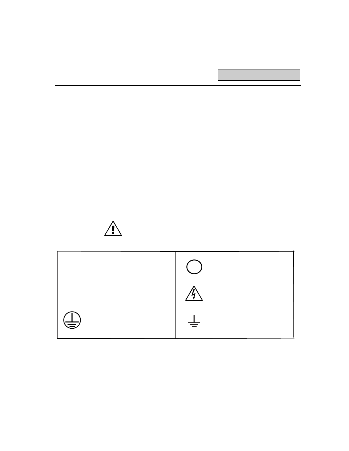
Safety Symbols Where these symbols or indications appear on the front or rear

panels, and in this manual, they have the following meanings:

CAUTION: Refer to accompanying documents (for Safety-related information). See elsewhere in this manual wherever the symbol is

present, as indicated in the Table of Contents.

On (Supply) Off (Supply)

Alternating Current Only CAUTION, Risk of electric shock

Protective Conductor Terminal Earth Terminal

WARNING Denotes a hazard. If a WARNING is indicated on the instrument,

do not proceed untils its conditions are understood and met.

1-4

Any use of this instrument in a manner not specified by the manufacturer may impair the instruments safety protection.

The WaveStation has not been designed for use in making direct measurements on the human body. Users who connect a WaveStation directly to a person do so at their own risk.

Power Requirements The WaveStation operates from a 115 V (90 to 132 V) or 230 V

(180 to 250 V) AC (~) power source at 47 Hz to 63 Hz. No voltage selection is required, since the instrument automatically adapts to the line voltage present.

The power supply of the WaveStation is protected against shortcircuit and overload by means of one internal 5.0A/250 V ~, "T" rated fuse. The fuse is not replaceable by the user.

The WaveStation has been designed to operate from a singlephase power source, with one of the current-carrying conductors (neutral conductor) at ground (earth) potential. Maintain the ground line to avoid an electric shock.

None of the current-carrying conductors may exceed 250 V rms with respect to ground potential. The WaveStation is provided with a three-wire electrical cord containing a three-terminal polarized plug for mains voltage and safety ground connection. The plug's ground terminal is connected directly to the frame of the unit. For adequate protection against electrical hazard, this plug must be inserted into a mating outlet containing a safety ground contact.

Power On Connect the WaveStation to the power outlet and switch it on by

pressing the power switch located on the front panel. After the instrument is switched on, a self test is peformed. The full testing procedure takes approximately 30 seconds, after which time a display will appear on the screen.

Do not exceed the maximum specified input voltage levels. (See appendix B for details.)

Warning

Installation and Safety

1-5

Installation and Safety

Risk of electrical shock: No user serviceable parts inside. Leave repair to qualified personnel.

Cleaning And Maintenance Maintenance and repairs should be carried out exclusively by a

LeCroy technician. Cleaning should be limited to the exterior of the instrument only, using a damp, soft cloth. Do not use chemicals or abrasive elements. Under no circumstances should moisture be allowed to penetrate the WaveStation. To avoid electric shocks, disconnect the instrument from the power supply before cleaning.

Service Procedure Refer any servicing requiring removal of exterior enclosure panels

to qualified LeCroy service personnel. Be prepared to describe the problem in detail. Prior to returning a unit please obtain a Return Authorization Number (RAN) from the LeCroy Customer Care Center in New York at (914) 578-6020 or the LeCroy office nearest you.

If the product is under warranty, LeCroy will at its option, repair or replace the LW400 Series at no charge. For repairs after the warranty period, the customer must provide a Purchase Order Number before the service engineer can initiate repairs. The customer will be billed for the parts, labor and shipping..

Shipping Guidelines 1. First attach a tag to the instrument which indicates:

a. Return Authorization Number b. Purchase Order number c. Owners name and complete address d. The service required including detailed operational problems e. Person to contact for confirmation (include phone number)

2. Ship the unit in its original packaging.

3. Protect the finish by carefully wrapping the unit in polyethylene sheeting.

4. Place adequate dunnage or urethane foam in the container (approximately 4 inch depth) and place the wrapped unit on it. Allow approximately four inches of space on all four sides and the top of the unit.

5. Fasten the container with packaging tape and/or industrial staples. Address the container to LeCroys service location and include your return address.

CAUTION

1-6

Getting Started

How To Use This Manual

The LW400 Series arbitrary waveform generator is designed to be operated without having to refer to this manual. This is made possible by the intuitive controls and guiding menus. Most of the arbitrary waveform generator functions are accessed using the Operation Keys clustered around the rotary knob. The other push buttons give access to the useful new features offered by this innovative instrument. A built-in Help library is provided for instant aid in answering questions while operating the AWG.

It is suggested that this manual be used to:

1. Gain an overview of the instrument

2. Familiarize you with the terminology

3. Provide detailed descriptions of the various functions

4. Illustrate the use of the new features of the instrument

Perhaps the best way to use it is to read through the early sections and then browse through the later chapters in order to become familiar with the LW400s capabilities. The Table of Contents is organized so that you can find the right information by locating the things you want to do.

*Note: The LW400 Series includes the LW420, LW420A, and LW420B dual channel and the LW410, LW410A, and LW410B single channel arbitrary waveform generators (AWGs). At times the designation LW400 is used to describe features common to all models. At other times specific reference is made to the LW400A and the LW400B Series.

WaveStation Arbitrary Waveform Generator The LeCroy LW400 makes it easy to create and edit waveforms

The LW400 combines complete on board word proccessor like cut, copy and paste, waveform editing with live waveform feature manipulation and waveform generation. Salient benefits include:

1. 100 psec feature placement resolution

2. 400 MS/s maximum sample clock for each channel

1-7

Getting Started

3. Sample Clock:

LW400 series sample clock rate is selectable within five decade ranges as describedsee chapter13

LW400A and the LW400B series sample clock is continuosly variable from 6 KHz to 400 MHz with a 1 Hz resolutionsee chapter 13

4. 100 MHz analog bandwidth

5. Fast Switch Group Sequence mode switches waveforms in < 11 ms minimizing test execution time.

6. 1 channel (LW410/LW410A/LW410B) and 2 channel (LW420/LW420A/lw420B) versions

7. Live update of waveform output

8. Stand alone design, no PC required

9. Waveform Data formats for Spreadsheets, PSpice, MathCad, MatLab, ASCII, and others

10. Up to 1 megabyte of playback memory (256 k standard)

11. Hard Disk of >400 Mbyte standard

12. 3.5 DOS compatible floppy disk for waveforms, sequence, equators, and projects, file transfer and storage

13. GPIB

14. SCPI compatible command set

15. Centronics hard copy interfaces

16. Internal Asynchronous noise source on the LW400 and LW400A series (not available on the LW400B series).

1-8

Getting Started

Accessories Supplied This Operators Manual

Remote Programmers Manual Power Cord for country of destination Protective Front Cover Firmware Installation Disk

Available Accessories

LS-RM Rackmount Kit LS400-SM Service Manual LS-CART Oscilloscope Cart LS-TRANS Hardshell Transit Case LS-SOFT Softshell Carrying Bag DC-GPIB 2 meter GPIB cable

Options

LW420-ME2 1 Mbyte Memory LW410-ME2 1 Mbyte Memory LW400-HD1 >400 Mbyte HDD LW400-09A Digital Output

Organization This manual is organized by application topics (e.g.,VIEWING WAVE-

FORMS and WAVEFORM EDITING) in order to provide rapid access to those areas of most use. When specific information concerning the operation of a particular push button or control is needed refer to the index of this guide or use the LW400 built-in HELP facility.

Using the Front Panel Controls The LW400 Getting Started Guide, which follows, describes the

basic operation of the LW400 series arbitrary waveform generators. Use it interactively with the tutorial in section 2 for a fast introduction to LW400 operations.

1-9

Getting Started

Welcome to the LeCroy WaveStation LW400 arbitrary waveform generator (AWG) Getting Started Guide. This guide offers a quick overview of basic LW400 operations. The Getting Started Guide is intended for a fast introduction or a brief review, more complete details are available in the following sections of the LW400 Operators Manual.

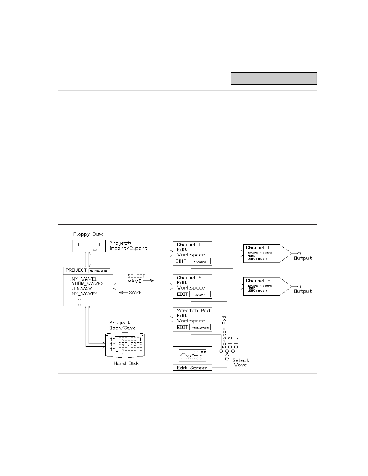
The WaveStation Concept

The WaveStation Concept is unique among arbitrary waveform generators in that it is designed to make waveform creation an interactive process. Waveforms can be created and modified continually with an observable, live response at the outputs.

The best place to start when learning to use the LW400 is to look at the conceptual block diagram, shown below.

Figure 1.2 Block Diagram

1-10

Central to the operation of an AWG is waveform creation and modification. This operation is done in the WaveStations editor which includes 3 workspaces. The channel 1 and channel 2 edit workspaces drive the respective outputs. The connection is direct and permits live updates of the output as the waveform is changed. The scratch pad area is an off-line, utility edit workspace. The EDIT control group on the front panel provides access to operations in the edit work spaces. Waveform selection, creation, and modification are all EDIT functions.

When a workspace is selected the current waveform contents are displayed on the internal CRT display. The VIEW control group provides control of the display parameters, time and voltage cursors, as well as hardcopy operations.

The output operations, like filtering and the addition of additive white noise, are controlled by the CHAN1 and CHAN2 controls.

The SAVE and PROJECT controls are used to move waveforms between the hard disk or floppy disk and the edit workspace. In addition to its waveform file management role PROJECT includes control of system related operations such as the real time clock and control of the remote interfaces.

Getting Started

1-11

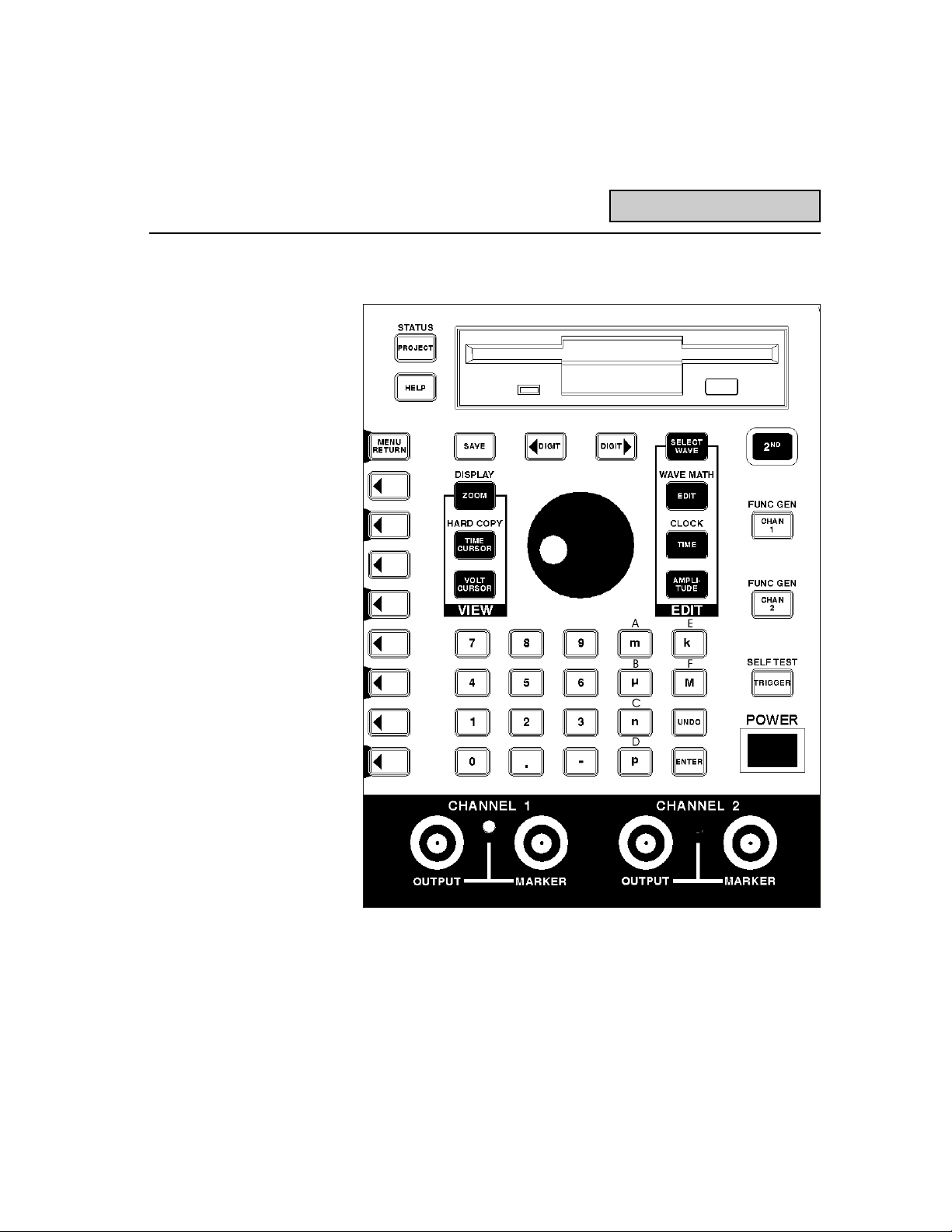
Front Panel Controls

LW420 Front Panel Layout

*Note the front panel of the LW410/LW410A is similar to the LW420/LW420A except that all controls related to channel 2 are removed.

Figure 1.3 Front Panel Layout

1-12

The LW400 WaveStation is a menu driven instrument. Push button controls on the front panel bring up related menus on the CRT display. The LW400 is controlled through the selection and/or entry of the desired parameters in the menus.

1. The controls on the LW400 front panel are divided into functionally related groups. For example:

The VIEW Group controls display related functions including hardcopy and the measurement of waveforms on the CRT Screen.

The EDIT Group controls waveform selection, editing, and modification.

The CHAN 1 and CHAN 2 buttons are used to control the channel related elements of the output such as turning channel output on or off, adding noise, or setting the output channel bandwidth.

2. The rotary control knob is used to select menu items or to scroll through numeric parameters within a menu item. The DIGIT select buttons set the rate of change of the rotary knob by selecting the digit of the numeric value to be modified.

Front Panel Controls

DISPLAY

1-13

3. The numeric keypad allows precise entry of numeric data into menu fields. Unit multiplier, enter keys p, n, µ, m ENTER, k, and M are used to attach the appropriate unit multipliers to the values being entered.

4. Dedicated controls are permanently labeled to indicate their function.

5. Dual function controls have a secondary function indicated by a red label printed above the control. The second function is accessed by first pressing the red push button labeled 2ND and then pressing the desired button.

6. Information on the function of each front panel button is readily available by pressing the Help button followed by the desired button or softkey.

7. The functions of the Menu or Softkeys, located adjacent to the CRT display, are indicated by menu labels shown on the display.

8. The rotary knob symbol appearing adjacent to a softkey label, on the CRT, indicates that the parameter described in the label may be varied using the rotary knob.

The keypads symbol appearing next to a softkey label, on the CRT, indicates that the parameter described in the label can be entered or changed using the front panel numeric keypad.

9. Softkey labels with a shadow box effect, such as the Marker label in the figure above, have additional menu items behind the label. Pressing the corresponding softkey again will list all the choices for that item.

Front Panel Controls

1-14

The LW400 Display The main elements of the LW400 CRT display are shown in the

figure below. The display annotation summarizes the current state of the generator including the date and time. Hardcopy capabilities allow the CRT display to be saved to a printer, plotter, or graphics file for notebooks or test procedure documentation.

The Display

Figure 1.4

Waveform Locator

Trigger Mode

1-15

Rear Panel Connections

Note: The digital output connectors for ECL and TTL are not present if the LW400-09A Digital Output option is not installed.

1-16

Using the LW400 as a Function Generator The LW400 includes a function generator mode offering

Sine, Square, Triangle, Ramp, Pulse, DC, and Multi-tone waveforms. The frequency of the periodic waveforms can be swept linearly or logarithmically using user entered sweep rate, and start/stop frequencies.

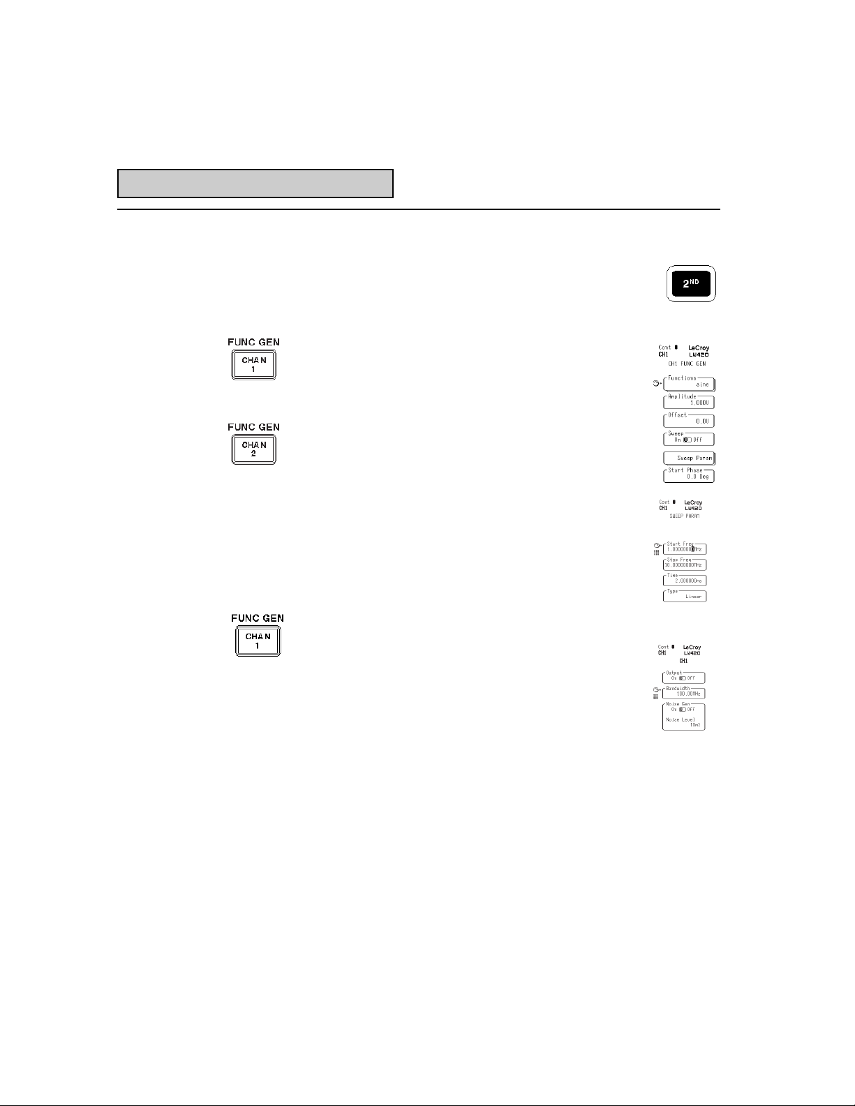
1. Select the function generator mode by pressing the red 2nd button and then selecting the desired channel. The Function Gen menu will be displayed allowing the selection of desired waveform, amplitude, offset, start phase, and frequency by means of the softkeys and/or numeric keypad.

2. Pressing the menu softkey labeled Sweep will alternately turn the frequency sweep on and off as indicated by the toggle switch icon. Pushing the Sweep Param menu key allows control of the sweep parameters.

3. Pressing the Chan 1 (or 2) button on the front panel allows access to the CH1 (or 2) menu.

4. The channel 1 (or 2) output can be turned on or off using the menu key labeled Output.

5. The bandwidth of either channels output can be controlled in decade steps from 10 kHz to 100 MHz. Bandwidth is automatically selected but the user may choose to override this selection.

6. Gaussian white noise can be added to the signal as a percentage of the peak to-peak signal level.

LW400 as a Function Generator

1-17

Figure 1.5

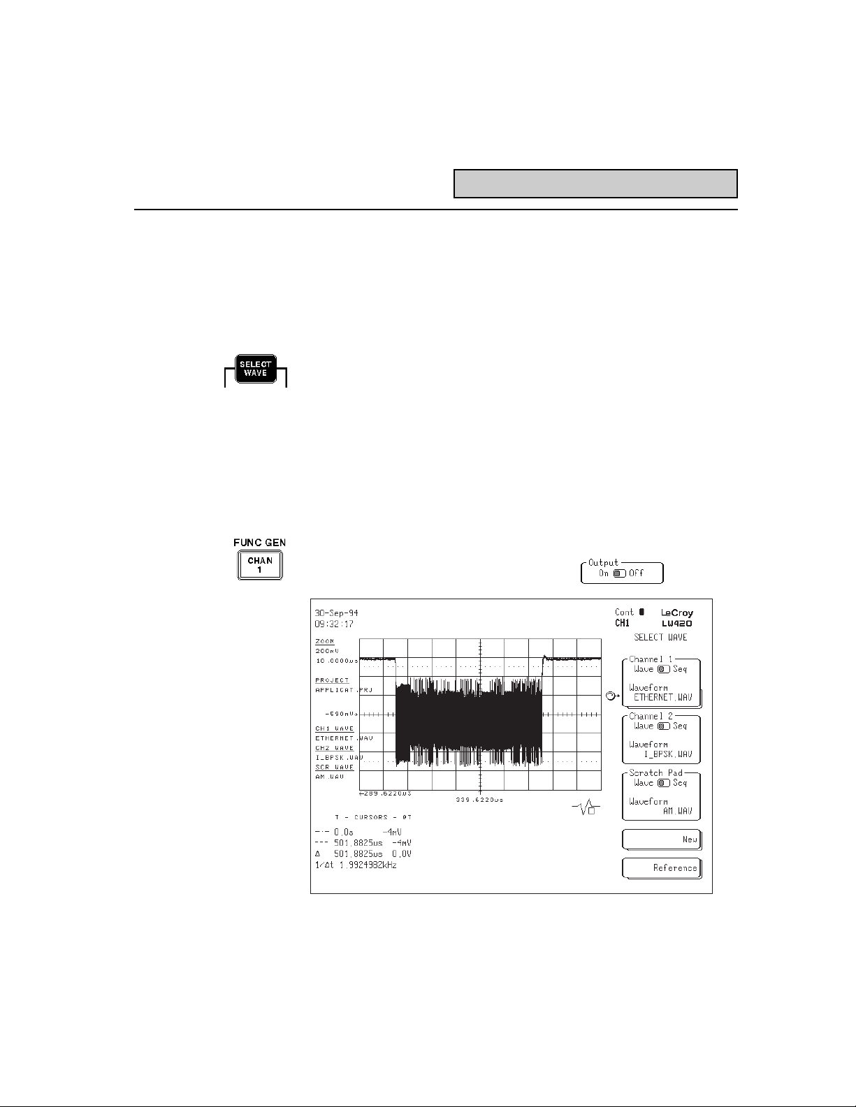
Generating Arbitrary Waveforms From Existing Waveform Files

Arbitrary waveforms can be generated from an existing waveform file or from a sequence of files described by a waveform sequence. The EDIT group on the front panel is used to select an existing waveform and output it.

1. Depress the SELECT WAVE button in the EDIT group.

2. Press the menu key corresponding to the waveform label in either Channel 1 or Channel 2. Use the rotary control knob to select the desired waveform filename which will be displayed and simultaneously output, as shown in figure 1.5. Its that simple!

3. The LED indicator next to the CHANNEL 1 (or 2) output connector is green when the waveform is being ouput and red when it is off. To control the output press the CHAN1 (or 2) button.

4. Push the menu button labeled Output, in the CH1 menu, to toggle the channel 1 output on or off.

Generating Arbitrary Waveforms

1-18

Recalling Other Waveforms or Sequences

Waveform files and sequences are stored in the LW400s internal hard drive under a dual level file system characterized by a project name and a waveform or sequence filename. This permits multiple users to each have their own set of independent waveform files. To recall a specific waveform you have to select the project it has been stored in and then the waveform or sequence filename.

1. Press the PROJECT button.

2. Push the button labeled Open in the PROJECT menu to see the existing project names.

3. Use the rotary knob to select the desired project, then press the Accept menu key.

4. Use SELECT WAVE, as shown previously, to see the available waveforms.

Recalling Other Waveforms

1-19

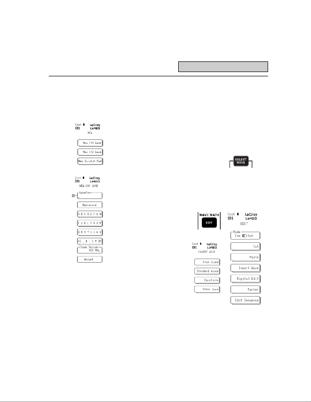
Creating a New Arbitrary Waveform Using Standard Waveforms The LeCroy WaveStation LW400 offers many techniques for

creating arbitrary waveforms. They can be imported from oscilloscopes, or common mathematics programs. They can be created from built in libraries of standard waveforms, or from mathematical equations. A full complement of waveform editing, modification, and array math capabilities allows existing waveforms to be used as sources of new waveforms. Waveforms are created in the currently open project, instructions for creating a new project are found in the following section.

1. Depress the SELECT WAVE button in the EDIT group.

2. Press the menu key marked NEW to create a new waveform name in either channel 1, or channel 2, or scratch pad.

3. Enter the desired waveform name, up to 14 characters long, then press the Accept softkey.

4. Press the front panel EDIT button to access the waveform and sequence edit functions.

5. Press the softkey labeled Insert Wave to access the waveform sources.

6. The Insert Wave menu allows the choice of acquiring the waveform from a digital oscilloscope, using the standard waves libraries, creating a waveform from an equation, or inserting another waveform.

Creating a New Waveform

1-20

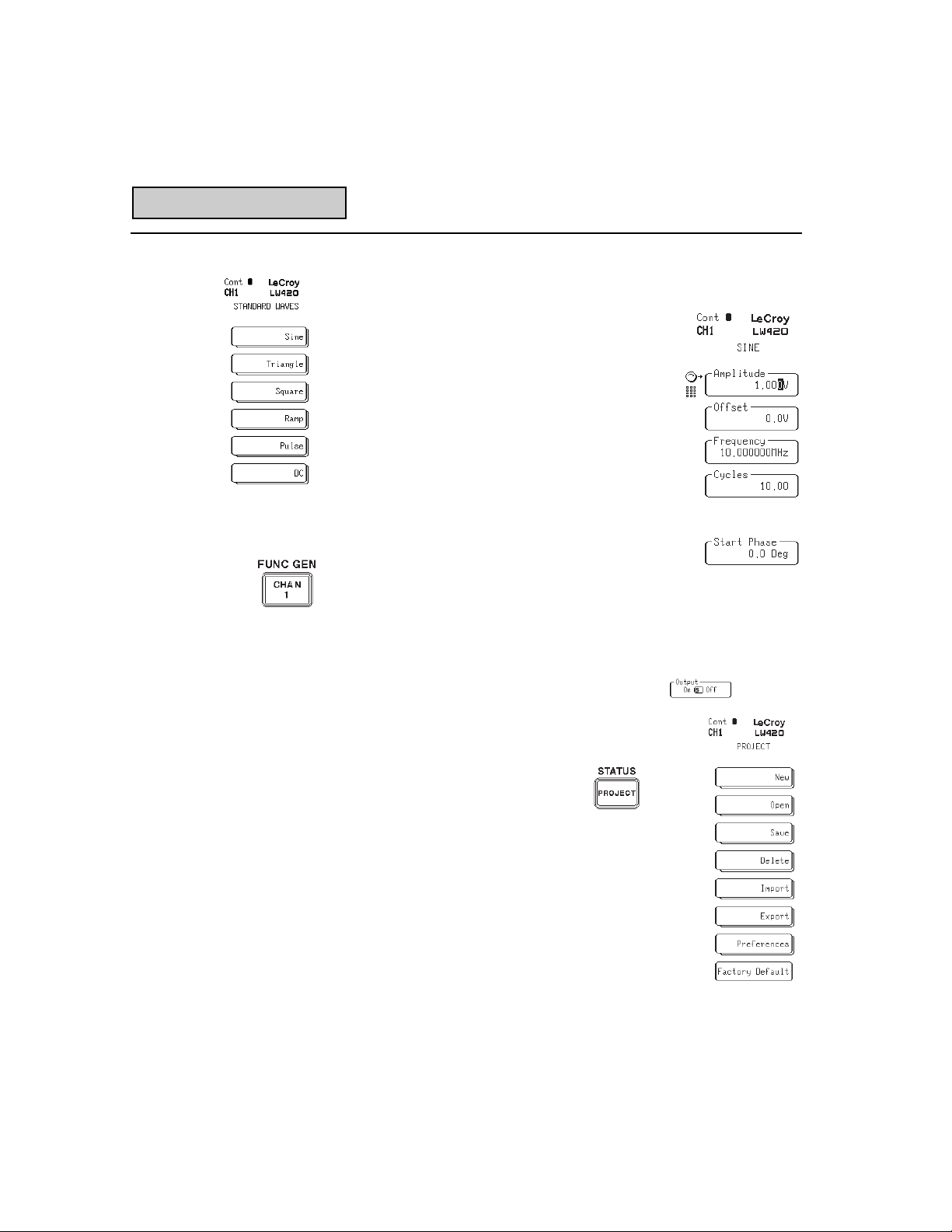
7. Press the menu key corresponding to the Standard Waves label. The LW400 will display a menu listing the standard waveform library.

8. The Sine menu, typical of the standard waveform setup menus, shows the waveform parameters that are available to control the standard waveform.

Select the menu softkey adjacent to the desired parameter and then use the rotary knob or the numeric keypad to enter the value needed. After all the parameters have been entered, press the Accept softkey to create the waveform.

9. The LED indicator next to the CHANNEL 1 (or

2) output connector is green when the waveform is being output and red when it is off. To turn the output on press the CHAN1 (or 2) button.

10. Push the menu button labeled Output, in the CH1 (or 2) menu, to toggle the channel 1 (2) ouput on or off.

Starting a New Project Projects provide individual work and storage areas,

especially helpful when multiple users share the AWG. To create a new project:

1. Press the PROJECT button.

2. Press the NEW softkey to enter a new project name, just as the waveform name was entered previously, and then press the Accept menu key.

New Project

1-21

Saving a Waveform After creating a new waveform it is a good practice to save the

waveform to the LW400s internal hard drive. The waveform is stored in the current project with a user assigned filename.

1. Press the SAVE button on the front panel to display the SAVE WAVEFORM menu.

2. The name of the currently selected waveform will appear in the menu item labeled Waveform. To save the waveform using this name press the menu keyed marked Save It.

3. To change the name of the waveform, press the menu key labeled Save As. This will bring up the SAVE AS menu allowing the entry of a new waveform file name. After renaming the waveform press the Accept menu key.

New Project

1-22

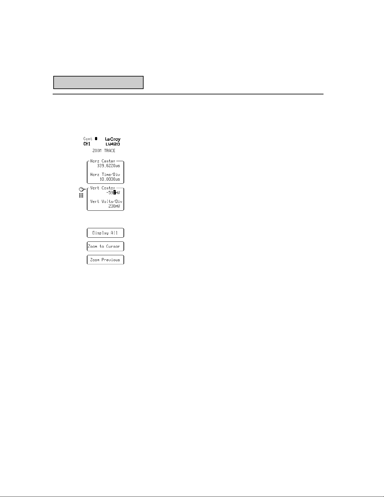
Using Display Zoom The display zoom controls are used to setup the display horizontal

and vertical scaling and position. These controls only affect the display of the waveform and not the waveform itself.

1. Push the front panel ZOOM button to display the ZOOM Trace Menu.

2. Pressing the softkeys labeled Horz Center, Horz Time/Div, Vert Center, and Vert Volts/Div allows the respective display parameter to be set using either the rotary knob or the numeric keypad.

3. Pressing the menu key marked Display All will automatically scale and position the waveform so that all of it is displayed.

4. The Zoom to Cursor menu selection will automatically scale and position the portion of the waveform between the left and right time cursors to fill the display area between 10% and 90% of the horizontal axis.

5. Selecting the Zoom Previous softkey restores the last zoom setting. This is used to quickly toggle between alternate display settings.

Display Zoom

1-23

Using Display Controls to Setup the Waveform Display The Display controls are used to setup the type of display, the

display Grid Style, and the waveform and grid intensity.

1. The display control menu is accessed by first pressing the red 2NDbutton on the front panel followed by pressing the DISPLAY/ZOOM button.

2. Pushing the menu key labeled Type allows the selection of one of 4 different grid types. Pressing the Type menu key a second time will show all the available selections.

3. In a similar manner, the LW400 display can be setup in any of 3 different grid styles using the Grid Style menu key.

4. Pressing the menu key labeled Intensity allows the intensity of the displayed waveform and its associated annotation to be varied using the rotary control knob or the numeric keypad. The range of intensity values is from 1% to 100%.

5. Similarly, the Grid Intensity softkey allows the intensity of the selected grid to be varied between 1% and 100% using the keypad or rotary knob.

6. Two system related display functions, the Screen Saver and the Time/Date display, are controlled using the System Preference menu. Since these are seldom used controls. They are grouped with other system related controls within the project group. This is described in the section on setting the system configuration.

Setup Waveform Display

1-24

Using Time And Voltage Cursors The dual time and voltage cursors of the LW400 provide calibrated

readout of the time or voltage amplitude of any position on a waveform. Both absolute and relative measurement readouts are shown on the LW400 display. Time cursors also are used to select specific regions, for all edit operations.

The adjacent figure shows both the time and voltage cursors. The waveform values at each cursor are displayed in the cursor readout field in the lower left corner of the CRT screen.

1. Push the TIME CURSOR button on the front panel to display the TIME CURSOR menu.

2. The menu key marked with Time Cursors toggle switch icon is used to turn the time cursors on and off. The default condition is On.

Figure 1.6

Cursors

Volt Bottom Cursor

Volt Top Cursor

Time Right Cursor

Time Left Cursor

1-25

3. In the track mode the right time cursor follows the left time cursor by a constant, user set, Delta. The track mode is controlled by the menu key labeled Track. The track toggle switch icon shows the state of the track mode.

4. The Time Left and Time Right menu keys are used to select and position the respective time cursors using the rotary knob or the numeric keypad. Time Cursor locations are entered in seconds.

5. Pressing the menu key marked Select All will move the left and right time cursors to the beginning and end of the waveform, respectively. Note that if the waveform extends beyond the

display the cursors may seem to disappear.

6. The Cursors to Grid menu key is used to bring the cursors to fixed positions on the current display. Pressing this menu key will force the left cursor to the 10% point and the right cursor to the 90% point of the display.

7. Depressing the menu key labeled Cursor to end will position both left and right time cursor at the end of the waveform.

8. Press the VOLT CURSOR button on the front panel to display the VOLT CURSOR menu.

9. The menu key marked with Volt Cursors toggle switch icon is used to turn the time cursors on and off. The default condition of the Voltage Cursor is Off.

10. In the track mode the top voltage cursor follows the bottom voltage cursor by a constant, user set, amplitude difference (Delta). The track mode is controlled by the menu key labeled Track. The track toggle switch icon shows the state of the track mode.

The Volt Top and Volt Bottom menu keys are used to select and position the respective voltage cursors using the rotary knob or the numeric keypad. Volt Cursor locations are entered in units of Volts.

Cursors

1-26

11. The Cursors to grid menu key is used to bring the voltage cursors to fixed positions on the current display. Pressing this menu key will force both the top and bottom cursors to first major graticule division inside the upper and lower limits of the display. The figure below shows the positions of both the Time and Volt cursors after pressing the Cursors to grid menu keys.

Cursors

Figure 1.7

Volt Top Cursor

Volt Bottom Cursor

1-27

Using The Live Waveform Modification Capabilities` The waveforms from the LW400 can be modified from the front

panel while the waveform is being output. Live output modification includes the ability to change all or part of a waveform. The amplitude, offset, duration, position, or delay (phase) can be modified as you watch the output on an oscilloscope. Waveform features can be shifted in time by as little as 100 ps. The adjoining screen display provides examples of some of the manipulations possible.

Figure 1.8

Waveform Modification

1-28

1. Recall or create the waveform that is to be modified.

2. Use the time cursors to bracket the feature or waveform segment to be modified.

3. To delay, move, or modify the duration of the waveform press the TIME button on the front panel to display the TIME menu.

4. Pressing the menu key labeled Duration allows the duration of the waveform feature, between the time cursors, to be varied using the rotary control knob or the numeric keypad.

5. Pressing the menu key marked Mode will change the toggle switch icon, alternating between the insert (Ins) and overwrite (Ovr) modes. If the duration is varied in the insert mode, all waveform data to the right of the feature being changed will move by the same time difference. In the overwrite mode the data to the right of the area being modified will be replaced, if duration is increased. In overwrite mode the overall duration of the waveform remains constant.

6. To move the selected waveform feature, press the menu key labeled Move. The selected area can now be moved horizontally under the control of the rotary knob or the numeric keypad. The LW400 captures and stores the original waveform segment for such calculations. As the selected region is moved signal processing techniques are applied to minimize discontinuities at the boundaries. The Capture Feature menu key allows the user to capture a different reference feature if desired.

The LW400 normally captures the feature for you and there is no need to push this button. This button is only needed to override normal capturing. For instance, if one pulse is moved on top of another and now it is desired to move the two pulses using this button will capture the new feature.

Waveform Modification

1-29

7. Pressing the menu key labeled Delay allows the selected feature to be delayed in time using the rotary control knob or the numeric keypad. Waveform elements to the right of the selected region will move by the same time delay increment.

8. To change the amplitude related parameters of the selected segment press the AMPLITUDE button on the front panel to display the AMPLITUDE menu.

9. Amplitude changes can be entered by controlling the amplitude, median value, maximum, or minimum amplitudes of the selected waveform segment. Pressing the menu key with the desired parameter name allows it to be controlled using the rotary knob or from the numeric keypad.

10. Pressing the UNDO button in the numeric keypad on the front panel will restore the waveform to the state it was in before the AMPLITUDE or TIME menu was entered.

Before the undo operation is executed the LW400 will put up a warning message confirming the operators intent to undo the changes.

Modification Capabilities

Figure 1.9

1-30

Triggering And Markers The LW400 has 4 triggering modes to provide flexible timing and

synchronization of the output waveforms. Each output channel includes a marker output which can be set up to provide a custom timing signal to the device or system using the AWG output waveform. The marker output can produce up to 128 user set edges or a clock output with user set frequency.

1. Press the TRIGGER button on the front panel to display the TRIGGER menu.

2. The trigger modes are selected using the menu key labeled Mode. Pressing this key a second time will show the four available trigger modes.

Continuous mode is a free running mode.

Single mode outputs the waveform once for each trigger

input.

Burst mode outputs an integer number of repetitions of the waveforms, as set in the Burst Count field of the trigger menu, for each trigger received.

The Gated trigger mode produces and outputs continuously as long as a gating signal, applied to the external trigger input, exceeds the preset trigger level. When the gating signal no longer exceeds the trigger level, the current waveform is output to completion and terminated.

Trigger sources include the external trigger input, manual trigger and trigger via the GPIB interface. The external trigger level and slope are entered in the Level and Slope fields of the TRIGGER menu. The external trigger input is mounted on the front panel. Triggers may also be initiated manually, by pressing the menu key marked Manual.

Triggering

1-31

3. Marker outputs, for each channel, offer a very flexible method of providing timing signals synchronous with the output waveform. Each marker is independently programmable with a timing resolution of one sample clock and is associated with a specific waveform. To edit or change the marker, press the SELECT WAVE button and use the SELECT WAVE menu to select or create a new waveform in either Channel 1, 2 or scratch pad.

4. Press the EDIT button on the front panel and select the Marker menu item from the EDIT menu. The MARKER menu will be displayed along with the marker waveform. The following figure shows a typical display using the dual grid display type.

5. The marker Output Level menu key is used to select either TTL or ECL logic levels for the marker signals.

Figure 1.10

Triggering

1-32

6. The marker Type menu key selects either a periodic clock or edge(s) as a marker type.

7. Pressing the Position menu key allows the positioning of a marker edge using the numeric keypad or the rotary knob. The time cursor tracks the position setting. The Set High and Set Low menu keys set the logic state starting at the current cursor position.

8. The clock marker type allows the clock frequency to be set by depressing the Frequency menu key. The frequency is settable from 10 Hz - 200MHz using the rotary knob or the keypad.

9. Similarly, the delay to the first clock edge is settable from 2.5 ns - 1 s using the First Edge menu field.

10. The Default Marker is a positive pulse, with a width of 31 sample clocks and a rising edge one sample clock from the begining of the waveform.

Configuration

Figure 1.11

1-33

Configuring the LW400 The system parameters of the LW400, including setup of remote

interfaces, setting the time/date, and disabling the screen saver, are all user settable.

1. Press the Project button on the front panel to display the Project menu

2. Push the Preferences menu softkey to view the Preferences menu.

3. Select the System softkey to access the System menu.

4. The Logo menu key is used to turn the LW400 logo, in the upper right corner of the display, off and on.

5. The Screen Saver softkey enables or disables the LW400 screen saver feature.

6. The GPIB menu keys provide access to the remote control interface setup menus.

7. Pressing the Set Time/Date menu key will display the Time & Date menu. This menu is used to set up the real time clock.

Configuration

2-1

INTRODUCTORY TUTORIAL

Introduction This tutorial is intended to give the new user of WaveStation his or

her first introduction. Further details on all operations are located in the remainder of the operators manual. This introduction is divided functionally into six main categories. They are as follows:

1. Creation of a simple arbitrary waveform

2. Display manipulation and zooming to see more detail

3. Positioning the Cursors

4. Live waveform manipulation

5. Simple waveform editing

6. Saving the Waveform

1. Creation of a Simple Arbitrary Waveform

Clearing the display We will create a waveform that consists of 4.75 cycles of a sine

wave followed by ten cycles of a square wave. The first step in the process is to ensure we start with a clean slate. The following steps will clear the channel 1 waveform display.

1, Push Select Wave

2. Push New

3. Push New CH1 Wave

4. Use the alphanumeric keys to enter the name new, (To enter a letter push the key that contains that letter in the list, then push the key with the letters symbol in it. For example, to enter the letter N first push the key that contains IJKLMNOP then push the N key.)

2-2

Tutorial

5. Push Accept after entering New

We now have a screen that shows no waveforms on it.

Creating 4.75 cycles of a sine wave

1. Push Edit

2. Push Insert Wave

3. Push Standard Waves

4. Push Sine

5. Push Cycles

6. Change the number to 4.75 (Use the keypad to enter 4.75. being sure to push enter on the keypad. Alternately use the rotary control to dial in the number 4.75).

Figure 2.1 The Blank Screen

2-3

7. Verify that all menu selections are as shown in figure 2.2. Make any necessary changes.

8. Push Accept

The screen of WaveStation should now show 4.75 cycles of a 10 MHz sine wave. It also shows some additional cycles very faintly. These show how the waveform segment connects to itself in continuous trigger mode. That is the two cycles before and five cycles after the highlighted five cycles are what comes before and after in continuous trigger mode.

Tutorial

Figure 2.2 The sine wave

2-4

Tutorial

Adding two cycles of a square wave

1. Push Time Cursor

2. Push Cursors to end (note: both cursors move to the right side

of the displayed waveform: all inserting of waves begins at the left cursor location which is now on the right side of the wave exactly where we want it)

3. Push Edit

4. Push Insert Wave

5. Push Standard Waves

6. Push Square

7. Select Base and set it for -500 mV (Type -500 followed by

m on the numeric keypad)

Figure 2.3 Add two cycles of square wave

2-5

8. Select Cycles and dial in 2 with the Rotary Knob

9. Verify that all menu items match those shown in figure 2.3

10. Push Accept

2. Zooming to see more detail

1. Push ZOOM

2. Push Horz Center

3. Using the Rotary Control dial in 400 nsec

4. Push Horz Time/Div

5. Select 100 ns (Use either the Rotary Knob or the numeric keypad

Tutorial

Figure 2.4 Result of Zooming

2-6

Tutorial

3. Positioning the Cursors

1. Push TIME CURSOR

2. Select Time Left

3. Turn the Rotary Knob and observe the cursor move

4. Select Time Right

5. Turn the Rotary Knob and observe the cursor move

6. Use the Digit keys (above the rotary knob) to change the sensitivity of the cursors

7. Set the cursors around some area of the waveform of interest to you, for example the second cycle of the sine wave

Figure 2.5 Result of Moving the Time Cursors

2-7

Tutorial

4. Live Waveform Manipulation

1. Push TIME in the Edit group

2. Select Duration

3. Use the Rotary Knob to change the Duration of the area of the waveform you selected

4. Select Move Feature

5. Use the Rotary Knob to slide your feature around

6. Select Duration

7. Experiment with the difference between the mode Ins and Ovr (notice overwrite removes data to the right of the region being expanded where as insert extends to total time [length] of the waveform.)

Figure 2.6 Live Waveform Manipulation

2-8

5. Simple Waveform Editing

The cursors should still be surrounding the feature you originally selected although you have probably stretched or compressed it.

1. Push Edit-the menu in figure 2.7 will be displayed.

2. Push Cut

3. Push Delete (your feature disappeared)

4. Push UNDO (on the keypad) and answer OK

(your feature is back)

5. Push Extract

6. Push UNDO followed by OK

7. Push Copy

8. Push Time Cursor

9. Move the Time Left Cursor to a new location

10. Return to the Edit Menu (Push Edit)

11. Push Paste

12. Push Accept

Tutorial

Figure 2.7

Edit menu

2-9

Tutorial

6. Saving Your Creation

1. Push SAVE button on the front panelthe menu shown in figure 2.8 is displayed.

2. Push Save Waveform

At this point, the waveform called NEW has been saved to the internal hard drive in the current directory or project. For a description of the project and directory structure see the section of the manual entitled Project Structure.

Figure 2.8

Saving the

Waveform

New

2-10

Tutorial

Final Exercise: Deleting the waveform New

1. Push Project

2. Push Delete

3. Push What and select Waveform

4. Push Waveforms and scroll until NEW appears

5. If you wish to delete NEW waveform select Delete.

Figure 2.9 Preparing to Delete New

3-1

WAVEFORM VIEWING

Waveform Viewing Viewing a waveform can have two different meanings. It can mean

viewing a waveform on the screen of the WaveStation, or viewing it on an oscilloscope. BNC to BNC cables are used to connect the AWG to an external oscilloscope such as a LeCroy 9354 digital oscilloscope. In general the signal or waveform appearing on the screen of the AWG is coming out the front panel BNC connectors and there is no further action required on the part of the user. (Except of course to set up the oscilloscope correctly: in the case of all LeCroy oscilloscopes, this means invoking the single keystroke auto setup).

The exceptions to this are if the channel being viewed is turned off or if it is the scratch pad editor, which is not connected to an output. If the channel is turned off, the LED between the front panel connector for the channel and the marker will be red indicating no output from that channel. To turn the channel on push the channel select button, such as CHAN 1 and then select output on using the upper grey softkey on the right side of the screen.

It is possible to have a different waveform displayed on the screen of the AWG than the one being viewed on the oscilloscope. For example, the oscilloscope can be connected to the output of channel 1 while the screen of the AWG is displaying the contents of the scratch pad or channel 2. This situation is rectified by pressing the button labeled SELECT WAVE and then selecting the desired waveform using the grey softkeys at the right of the display.

3-2

Select Wave

Triggering an external oscilloscope In order to produce a stable display on an oscilloscope, it is

frequently necessary to use an external trigger. The simplest way to do this is to use the marker output of the WaveStation to trigger the scope. Connect a BNC to BNC cable between the Marker output connector of the appropriate channel on the front of the WaveStation and the external trigger input of the oscilloscope. Set the oscilloscope trigger conditions of the external trigger, DC coupled, negative edge and set the threshold at approximately 300mv (the default marker is a TTL level pulse so, anything above a few hundred millivolts will do). The scope should now trigger and produce a stable display.

If the display is still not stable, make sure that the default marker is enabled. To do this, press EDIT and enter the Marker menu and push Default Marker. For further information, see the section of this manual titled MARKER.

WAVEFORM SELECTION

Figure 3.1 Result of Pushing Select Wave

3-3

GENERAL Selecting a waveform generally implies choosing the desired wave-

form to display or playback from a list of options. It may mean selecting a waveform for editing with live feature manipulation by editing one of the channels while it is active. It could also mean editing a waveform in the scratch pad memory so the results of the edit can be viewed without affecting the current state of the output. An additional function is the creation of completely new waveforms. Pushing the button labeled SELECT WAVE near the upper right side of the AWG rotary control knob causes the AWG to enter a menu from which these various options can be exercised.

Help! Where is my waveform? (Changing Projects)

If the desired waveform does not seem to be available, it is possible that it is stored in a different PROJECT than the one currently active. This may be remedied by pushing the button labeled PROJECT on the left of the floppy disk drive and opening the correct project. See the section on Project Structure for a more detailed description of projects and waveform management.

Channel 1/Channel 2 In the box labeled channel 1 or channel 2 there are two choices:

Wave/Seq and Waveform*. The former is a toggle switch that chooses whether or not the output of the selected channel is to be a simple waveform or a sequence of waveforms . See the section on Sequence Waveforms for a detailed explanation.

*NOTE: For this discussion it is assumed that the toggle switch has been set to WAVE.

Select Wave

Table 3.1 Summary of Select Wave menu

Channel 1 Select Waveform or Sequence for Channel 1 Channel 2 Select Waveform or Sequence for Channel 2 Scratch Pad Select Waveform or Sequence for the Scratch pad New Select a New Wave Reference Select A Reference Wave

3-4

The second choice is Waveform. Pushing the associated grey softkey will cause the Rotary Knob symbol to attach to the waveform select function. Turning the rotary knob will scroll through the list of available waveforms. Alternately pushing the associated grey softkey again will cause the AWG to display the list of available waveform options on the left side of the screen. The associated softkey can be pushed to select the desired waveform. As described previously, if the waveform desired is not in the list, perhaps it is stored in a different project.

Notice that after selecting a waveform for channel 1 or 2, the corresponding waveform is now displayed on the screen of the AWG. This waveform is now appearing at the output of the BNC connectors as described above provided the output is enabled.

Figure 3.2 Selecting the Wave from a list

Select Wave

3-5

Scratch Pad The Scratch Pad has the same selection options as Channel 1 and

Channel 2; however, it has a different functionality. The scratch

pad is not directly associated with an output channel. It is, as the name implies, a place to experiment with different waveform options before they are committed to an output. Waveforms can be edited in the scratch pad memory without affecting the state of the output of the AWG.

New This is the starting point for creation and naming of a totally new

waveform. Pushing the softkey labeled new activates a sub menu permitting selection of a new channel 1 wave, a new channel 2 wave or a new scratch pad wave as a new wave. Selecting one of these three options now causes the system to jump to its alphanumeric entry menu and permits the user to assign a unique name to this new waveform.

Note that alphanumeric entries may also be made via an IBM PC/AT compatible keyboard connected to the Auxilliary Control connector on the rear panel of the LW400. Entries from the keyboard are limited to upper case letters and numbers. The backspace key may be used to delete text.

Select Wave

Reference

Selecting the Reference Often it is desirable to see a reference wave. For example, it may

be desirable to edit a waveform while viewing the original version of the waveform as it is being edited. The reference wave provides this ability. In the accompanying figure, a reference wave (bottom trace) is shown simultaneously as the WaveStation user prepares to Edit the active Waveform file (top trace).

Selecting Reference from the SELECT WAVE menu causes the WaveStation to enter a submenu from which it is possible to choose the reference wave. The choices are the same as for the channel 1 or channel 2 wave. There is an additional selection to Show Reference. Answering yes permits the reference to be viewed.

3-6

Reference

Figure 3.3 Viewing the Reference

3-7

Display

Figure 3.4 Setting up the display

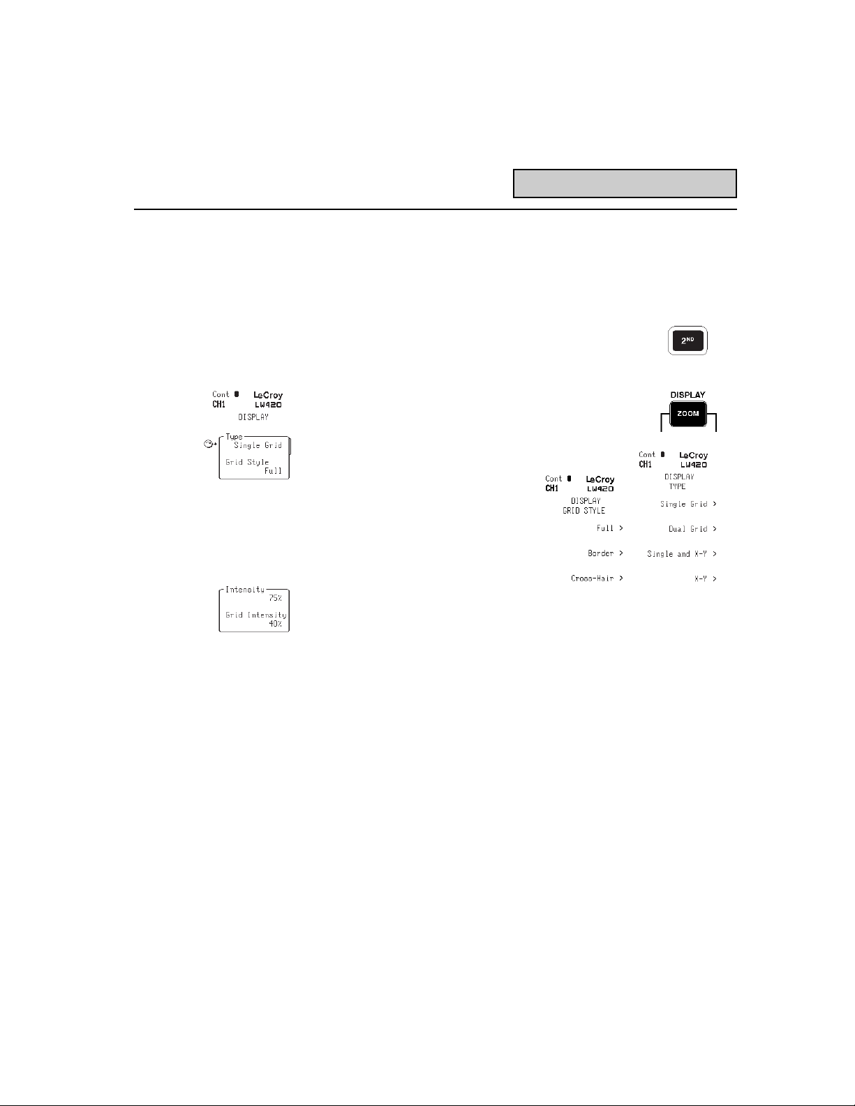
Splitting the Grid To have two grids as in the figure, it is necessary to enter the

display menu. Push 2nd followed by DISPLAY and under Type select Dual Grid and push MENU RETURN. For further details see the following section on DISPLAY.

Display The Display menu is used to setup the type of display, the grid

style, and the display intensities. Press the red 2ND button and then DISPLAY ( the alternate function of the ZOOM button). The DISPLAY menu, shown in the adjacent figure, will appear.

3-8

Display

Type The four display types available are Single, Dual, Single and X-Y,

and X-Y. Press the Type softkey to enable selecting the display type using the rotary knob. Pressing the softkey a second time will show all the choices along with individual softkeys for selection.

With Single grid, the selected waveform, or the selected waveform and the reference waveform can be displayed within the same grid.

The Dual grid splits the display into two grids. The selected waveform is displayed within the top grid. The reference waveform, if enabled by Show Reference switch in the REFERENCE menu, is displayed in the lower grid.

The Single and X-Y grid combines an X-Y display and a single display grid. The Reference waveform is plotted as the Y (ordinate) axis, while the Selected Waveform is plotted along the X (abscissa) axis. This arrangement permits waveform phase relationships to be investigated as shown in the accompanying figure.

Similarly, the X-Y grid provides a full screen view of the reference waveform plotted against the selected waveform.

Figure 3.5 X-Y Single Display

3-9

Display

Grid Style Full, Border, or Cross-Hair grids can be selected by pressing the

Grid Style softkey. The Full grid includes graticule lines at each major division in the 8 by 10 division display. The Border style eliminates all the grid lines except for an outer border. The Cross- Hair grid, as the name implies, consists of a set of perpendicular axes marked with major and minor division increments

Intensity The Intensity menu field is used to set the displayed intensity of

the waveforms and annotation. When selected, it is adjustable over a range of 1% to 100% using the rotary knob or by numeric entry from the keypad. Likewise, the Grid Intensity allows the user to adjust the brightness of the grid lines independently of the waveform traces.

3-10

Zoom

Figure 3.6 The Zoom Trace Menu

Zoom Pushing the operation key labeled ZOOM on the left of the rotary

control knob activates the menu that permits selection of the displayed time and amplitude scale factors (zoom factor). The ZOOM controls only affect the display of the waveform. The time base and amplitude settings of the waveform are not affected by these settings. There are two major selection fields in this submenu. They are Horizontal and Vertical. Each section has two additional selections: the value at the center and the appropriate scaling in time or volts per division. Pushing the appropriate grey menu button causes the rotary control to attach to the function selected. The rotary control is now used to change the value of the selected function. Whenever the rotary control is used to change a numerical value, the resolution of the digit being controlled can be changed by using the left and right digit button located above the rotary control.

3-11

Zoom

When a selected numerical quantity is lowered or raised until either the low or high limit is reached, an error message is printed on the screen of the AWG. This error message states for example, Cannot decrement this digit meaning that either incrementing or decrementing the selected digit will exceed the extreme limit for the field.

Display All Display All causes the entire waveform to appear on the screen. It

has the effect of undoing any expansions that have previously been invoked both in time and in amplitude. This will effect the display only, and not the current waveform or output.

Zoom to Cursor Zoom to Cursor will cause the region of the waveform between the

time cursors to expand and fill the screen between the 10% to 90% horizontal grid line.

Zoom Previous Toggles between the current and previous ZOOM setting.

3-12

Exercise Waveform selection and zoom

1. Connect the AWG to an oscilloscope

2. Push Project

3. Push the softkey next to Open

4. Select the project name APPLICAT.PRJ

5. Push Accept

6. Push Menu Return (this step can be skipped)

7. Push Select Wave

8. Push the grey soft key next to Channel 1 Waveform

9. Select PHOTO.wav

10. Push Menu Return (this step can be skipped)

11. Push ZOOM

12. Position Horizontal Center at 12 µs

13. Expand Horizontal Time/Div to 200 ns

14. Toggle Display All and Zoom Previous

Figure 3.7 The Result of Exercise 1

Exercise

4-1

LIVE WAVEFORM MANIPULATIONS

Cursor Manipulations Live waveform manipulation means selecting some feature of a

waveform and changing it while the output is also modified. This change does not occur in real time: there is some delay between feature manipulation in the AWG and a change in the state of the output which is proportional to the size of the area affected.

The first step in live waveform manipulation is to use the time cursors to select a region of interest in the waveform. This may also involve using the Zoom controls discussed previously. By using Zoom to expand the waveform a detailed examination and selection of waveform elements can be accomplished. This will help assure accurate results of a waveform manipulation of a specific feature.

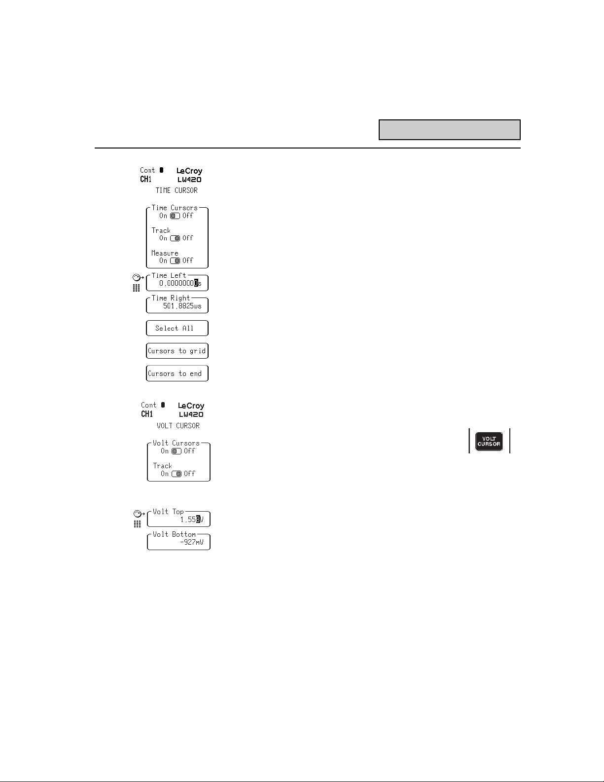
Time Cursors Pressing the Operation key labeled TIME CURSOR next to the

rotary control knob activates the menu depicted in figure 4.1 and summarized in table 4.1 below. The time cursors consist of two vertical bars that can be positioned on either side of a waveform feature in order to manipulate extract or delete that feature when

Figure 4.1 Time Cursor Menu

4-2

Time Cursor

editing. (See editing waveforms in section 6). The time cursors may not cross one another. Time cursors are used in all editing, functions and measurements. Measurements and Cut editing operations use both cursors while Paste and other Insert operations use the left Cursor.

Help ! Where are the Cursors? When the cursors are first turned on, it is possible that they are not

visible on screen. Try pushing the softkey labeled Cursors to Grid immediately. The reason the cursors may not be seen initially is they are located on a portion of the waveform that is outside the field of view. This can occur if, for example, the waveform has been previously expanded and recentered using the ZOOM controls. Notice it is possible to manipulate the cursors independent of viewing them: the AWG knows where the cursors are even if they are not being displayed. Similarly Cursors To End may move the cursors off the screen and outside the field of view if the present state of the expansion is such that the end of the waveform is outside the field of view.

Another reason the cursors may not be visible is because they are located directly over a display gradicule line. Turning the rotary control knob will bring the selected cursor into view.

Table 4.1 Summary of Time Cursor Operations

Time Cursor On/Off This toggle switch selection turns the timer cursors on or off Track On/Off With track set to On, the right cursor moves with left cursor at a fixed

time difference (DELTA) when the left cursor is selected and moved. Measure On/Off This toggle switch turns the measurements on or off Time Left Select this field to move the Time Left Cursor Time Right Select this field to move the Time Right Cursor Delta Change the delta between the cursors Select All Position the cursors to surround the entire waveform Cursors To Grid Move the cursors onto the grid (see discussion below) Cursors To End Move both cursors to the right end of the waveform

4-3

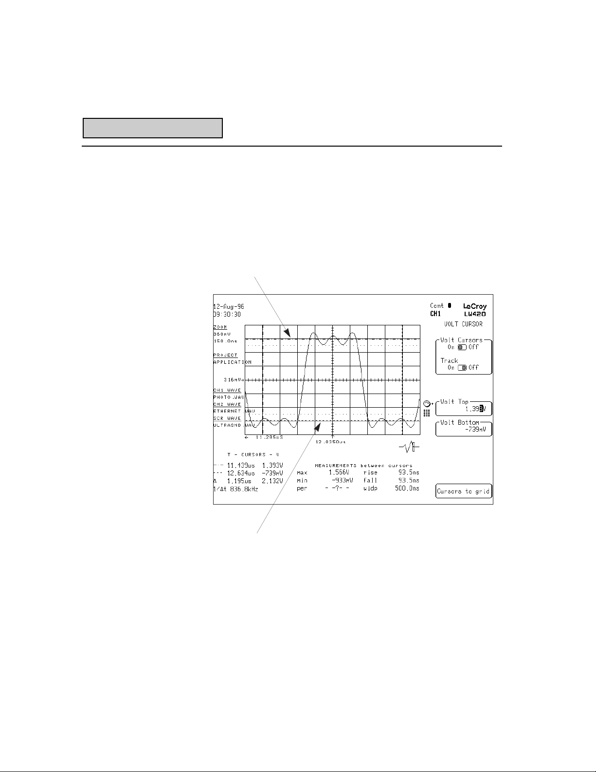
Measure When the measurements are on they will be displayed in the

bottom center of the screen (below the grid). Six measurements will be made: min, max, rise time, fall time, period (PER) and width (WIDP). Min will be the minimum amplitude between the Time Left and Time Right cursors. Max will be the maximum amplitude between the Time Left and Time Right cursors. Rise time and Fall time will be the first respective qualifying edge after the Time Left cursor and are 10% to 90%. Period will be the time between two odd numbered 50% crossings beginning with the 1st crossings after the left cursor. WIDP is the time between adjacent 50% crossings for the first positive pulse between the cursors. See Appendix A for more detail.

Voltage Cursors Pressing the menu selection key labeled Voltage Cursors next to

the rotary control knob activates the submenu seen in figure 4.2 and summarized in the table below. The voltage cursors consist of two horizontal bars that can be positioned up or down along the waveform. The voltage cursors may not cross one another. These cursors are used for making measurements on waveforms.

Voltage Cursor

Fig. 4.2 Voltage Cursor Menu

voltage cursors

4-4

Live Manipulations Many Time Editing operations are performed as quickly as possible

in response to user input. The LW400 attempts to compute the desired waveform immediately when the state is changed. If the requested state is changed again before the computation is completed, the partially completed computation is discarded and a new attempt to compute the desired waveform is begun.

If the waveform being edited is the active waveform for one of the channels, then it is automatically updated when the new waveform is computed. The output holds a data point from the previous waveform while the new playback image is being loaded. The playback of the new image begins at its first value.

Voltage Cursor

Table 4.2 Summary of Voltage Cursor Operations

Volt Cursor On/Off This toggle turns the voltage cursors on or off Track On/Off With Track set to On, the voltage cursors move together at a

fixed voltage difference (DELTA) when the top cursor is moved. Volt Top Select this field to move the top voltage cursor Volt Bottom Select this field to move the bottom voltage cursor Delta With track On, this is the voltage difference between the top

and bottom cursors Cursors To Grid Position the cursors on the grid from their current location

4-5

Time Edit Press the Time button in the Edit group to get the menu of figure

4.3. From this menu the duration of part or all of a waveform can be rescaled, or shifted (delayed) in time. Changing the duration of a region always expands or compresses it horizontally: vertical scaling is not affected.

Duration Stretches and compresses the waveform between the cursors hori-

zontally, in time. The left cursor remains in a fixed position and the right cursor moves to the left or right depending on the direction in which the rotary knob is turned. A number for duration can also be entered using the numeric keypad. As the right cursor slides in response to the input, the amplitude value at the right cursor remains fixed. The method of insertion depends on the selection of mode described below.

Note that using duration provides a quick way to rescale an entire waveform. Using the time cursors, select all, then change duration.

Time Edit

Fig 4.3 The Edit Time Menu

4-6

Time Edit

Mode In Overwrite Mode the length of the waveform doesnt change as a

region is rescaled: as the region expands, data to the right of the region is overwritten; as the region shrinks, amplitude of the rightmost point is replicated to keep the waveform length constant. In Insert Mode the waveform size increases and decreases as the region increases and decreases.

Move Feature Slides the region, or feature, between the cursors over the wave-

form. As the region slides, the waveform values are linearly superimposed on each other. The precision with which a feature can be placed is 100 psec.

Capture Feature As a waveform feature is moved the linear addition causes new

features to be formed. That is for example, a pulse sliding over another pulse and adding to it will cause a new pulse that is the sum of the two. If it is now desired to capture this new feature and move it, then press Capture Feature. The memory will now lose the old feature and begin to slide the new feature in its place.

Delay Takes the entire waveform starting with the left cursor and slides it

to the right or left by an amount equal to the value in the Delay field. This is done with a maximum precision, or resolution of 100 psec.

4-7

Time Edit

Fig. 4.4 Moving the feature in PHOTO.WAV

1. Refer back to Exercise 1 for Waveform Selection & Zoom

2. Press Time Cursor

3. Position the Time Left and Time Right Cursor around a small section of the waveform

4. Press Time in the Edit section

5. Select Move Feature and turn the Rotary Knob. Observe the effort on the oscilloscope.

6. Push UNDO on the keypad and answer ok

7. Select Duration and turn the Rotary Knob. Observe the effort on the oscilloscope.

8. Repeat step 6

9. Select Delay and change it with the Rotary Knob. Again, observe the effort on the oscilloscope.

10. Repeat step 6 to Undo your changes

Live Waveform Manipulation

4-8

Amplitude Edit Press the Amplitude button in the Edit group to get the menu of

figure 4.4. From this menu the amplitude of all or selected portions of the active waveform can be manipulated live.

Amplitude Edit

Figure 4.4 The Edit Amplitude Menu

Amplitude Sets the peak-to-peak amplitude of the waveform between the two cursors

with respect to the baseline.* The baseline is the line drawn between the

two cursors Median Sets the median voltage of the displayed waveform between the time cursors Max Voltage Sets the maximum voltage of the displayed waveform between the time

cursors Min Voltage Sets the minimum voltage of the displayed waveform between the time

cursors

Table 4.3 Summary of the Edit Amplitude menu

*Note: The baseline is the reference line shown on the display, connecting the points where two cursors intersect the waveform.If the baseline termination points are not of equal amplitude the baseline will be sloped.

4-9

Live Waveform Inversion Waveform inversion (i.e. multiply by -1) is available as an amplitude

edit function. As in all of the edit functions, the portion of the waveform between the time cursors is affected by the invert operation. It is possible to invert all or part of the waveform.

In the example shown in the top trace of the accompanying figure, the portion of the waveform between the time cursors has been inverted. The lower trace is the reference waveform, showing the original waveform. Note that the signal is inverted about the edit baseline (the line connecting the points on the waveform intersected by the time cursors). In this example the baseline is set to be 0 Volts.

Amplitude Edit

Figure 4.5 The Invert softkey in the Amplitude Edit menu

5-1

INSERT WAVE

Edit

Insert Wave Menu There are many different sources of waveforms available to the

user of the LW400 Series Arbitrary Waveform Generator. Waveform files may be transferred directly from a variety of oscilloscopes without the need for an intermediate computer. They may also be transferred from other LeCroy arbitrary function generators. Especially important to current users of LeCroy AFGs is the ability to transfer EasyWave files to the LW400. If a function can be described with an equation, then the built in equation editor should make entry relatively painless. Waveform files may be input in an ASCII format from any source. In addition, a variety of standard functions are available as a starting point for waveform creation.

All of these functions can be accessed from Insert Wave, as summarized in table 5.1.

Fig 5.1 The Edit Wave Menu

5-2

Insert from DSO

From Scope DSO Type This is the type of digital oscilloscope that the waveform will be

downloaded from. There are many available choices including oscilloscopes from LeCroy, Hewlett Packard, and Tektronix. Other oscilloscopes may be added by importing an appropriate digital oscilloscope configuration (DSO) file using the Import function in the Project menu.

GPIB Address This command does not set the address of the scope or the AWG.

It tells the AWG what address the DSO is already set for.

Table 5.2 Summary of Get From Scope menu options

DSO Type Selects from the list of available scopes Trace Source Selects which (DSO) Trace to get the waveform from DSO GPIB Address Selects the scopes GPIB address (see below) Preserve Time/Pts Preserve time resamples the data keeping the waveform duration

constant. Preserve points reproduce each sample acquired from the DSO but at the LW400s clock period

Request Control yes/no Set to yes if LW400 is installed in a system with another

GPIB controller on the bus.

Execute Transfers the waveform from the DSO to the AWG

Table 5.1 Summary of Sources from which Waves may be inserted

From Scope Waveforms can be inserted from a variety of scopes (Section 5.1) Standard Waves There are a variety of standard waves (Section 5.2) Equations The equation editor is described in Section 5.4 Other Waves Insert other waveforms from current project

5-3

Insert from DSO

Preserve Time/Pts This choice allows the operator to select between preserving the

shape in absolute time of a waveform that is being transferred or to preserve the number of points. For example, suppose a DSO has sampled a waveform at 200 Megasamples/second and the WaveStation is running at a clock speed of 400 Megapoints per second. Preserving time means the waveform coming from the scope is resampled to match the faster clock speed of the AWG and thus will have twice as many points.

Preserving points, on the other hand, means the reconstructed waveform will have twice the frequency content of the original waveform. This is because the reconstructed waveform will have the same number of points however; since the AWG is going twice as fast as the scope, the new points will be spaced closer together.

The choice to preserve the number of points has the potential to change the frequency content of a signal unless the WaveStation clock is adjusted accordingly but it preserves the exact shape of the waveform.

Figure 5.2 Insert From Scope

5-4

Insert from Standard Waves

Standard Waves A library of standard waves is available. Figure 5.2 shows the

menu selections available in the standard waves menu. The tables below summarize the characteristics of these waves.

Sine

Variable Range Resolution Default Value Amplitude (peak-to-peak) 0 mV - 10 V 1mV 1 Volt

Offset @ zero phase +5 V to -5 V 1 mV 0 Volts Frequency 1 Hz to 100 MHz 1 ppm 10 MHz Cycles 0.01 to 65 k 1 or 10 10 cycles Start Phase (see note below) 0 to 360 .05 degree 0 degree

Figure 5.3 Standard Wave Selection

5-5

Insert from Standard Waves

Square

Ramp

Triangle

Variable Range Resolution Default Value Amplitude (peak-to-peak) 0 mV - 10 V 1mV 1 Volt

Offset @ zero phase +5 V to -5 V 1 mV 0 Volts Frequency 1 Hz to 25 MHz 1 ppm 10 MHz Cycles 0.01 to 65 k 1 or 10 10 cycles Start Position 0 to 100% 1 m % 0.0 % Invert on/off off

Variable Range Resolution Default Value Amplitude (peak-to-peak) 0 mV - 10 V 1mV 1 Volt

Offset @ zero phase +5 V to -5 V 1 mV 0 Volts Frequency 1 Hz to 25 MHz 1 ppm 10 MHz Cycles 0.01 to 65 k 1 or 10 10 cycles Start Phase (see note below) 0 to 360 .05 degree 0 degree

Variable Range Resolution Default Value Amplitude (peak-to-peak) 0 mV - 10 V 1mV 1 Volt

Base +5 V to -5 V 1 mV 0 Volts Frequency 1 Hz to 50 MHz 1 ppm 10 MHz Cycles 0.01 to 65 k 1 or 10 10 cycles

Time Delay 0 ns to mem. length 1 ns 0 ns

Edge Time (risetime and falltime) 5 nsec to 500 ns 1 ns 5 ns

1. This range is given for the 400 MS/s clock rate. This range is scaled with the clock rate.

5-6

Insert from Standard Waves

Variable Range Resolution Default Value Level + - 5V 1mV 1Volt

Duration 10 ns to mem length 1ns 10 usec

1. This range is given for the 400 MS/s clock rate. This range is scaled with the clock rate.

2. Maximum period and width are related to the length of waveform memory. Numbers quoted are for 1 Mbyte memory.

Pulse

Variable Range Resolution Default Value Amplitude (peak-to-peak) 0 mV - 10 V 1mV 1 Volt

Base +5 V to -5 V 1 mV 0 Volts

1, 2

Period 10 ns - 2.5 ms 1 ppm 10 MHz

Cycles 0.01 to 65 k 1 or 10 10 cycles

1, 2

Width 0 to 2.5 ms 1 ns 5 ns

Time Delay 0 to memory length 1 ns 0 ns

Edge Time (risetime and falltime) 5 nsec to 500 ns 1 ns 5 ns

5-7

Edit Equation

Equations Any waveform that can be described by an equation using the 11

basic waveform functions, can be entered via the equation editor. This includes simple everyday functions like sine waves and pulses, and extends to very complex mathematical expressions. The equation editor provides an environment for entering, editing and calculating mathematical functions.

This section of the manual describes the equation editor and the associated functions and arguments.

Waveform Equation Notebook A separate publication called the Waveform Equation Notebook

gives examples of many functions and their associated equations. The Waveform Equation Notebook is included with this manual section.

5-8

Edit Equation

Select Line

This field allows a user to select one of the 16 lines in the equation. This is the equation line that is calculated. A valid line number can be entered using the numeric key pad or the rotary knob can be used to move the line cursor. The cursor will not wrap around from line 16 to line 1, it will stop at the extremes.

Figure 5.3 Edit Equations

Table 5.3 Summary of Edit Equation Options

Duration This is the duration of the waveform that is calculated Edit Equation Line Enter an equation on the selected line New Start or name an equation Open Get an already existing equation Save Save an equation Calculate Calculate the equation in the selected line and produce a waveform

5-9

Edit Equation

Edit Eqn Line On entering this menu the select line bar will go away and the text

cursor will appear at the beginning of the selected line. When the Functions, Operators, Variables, or Arguments field is pressed, the lists are expanded, allowing the user to choose a list item. When the list item is selected (by pressing the softkey next to the item) it will be inserted into the equation. Constants can be placed into the equation by using the numeric key pad. No attempt will be made to make sure that the equation is syntactically correct, it is solely up to the user. If an incorrect equation is calculated, the user will be told there is an error in the equation. References can be made to include other lines of the equation sheet by defining variables. The entire equation will be expanded (internally) but the expanded version must not exceed 1024 characters.

Figure 5.4 The Equation Editor

5-10

Edit Equation

Functions The following functions can be used in equations; Absolute

Value(ABS), Cosine(COS), Exponent(EXP), Integer Floor (FLOOR), Natural Logarithim(LN), Common Logarithim(LOG), Pulse (PULSE), Sine(SIN), Square Root(SQRT), Unit Step(STEP), Tangent(TAN). Since all these functions require a ( ) after the function name, it will automatically be inserted and the cursor will be placed between the parentheses.

Operators The available operators are; Add(+), subtract(), multiply (*),

divide( /), group ( ), comma (,) and raise to a power( ^).

Variables You can define a variable in the form of X# = <any valid equation

including constants>, where # ranges from 1 to 16. These variables can be used in the middle of another equation, e.g. X1 + X2.

Arguments Includes: 2*PI*T, T, PI, NOISE and GNOISE. NOISE returns a

pseudorandom series of values with uniform amplitude distribution. GNOISE returns a pseudorandom sequence with Gaussian distributed amplitude values. Note: T = 0 at the left cursor.

Figure 5.5 The Functions List

5-11

Edit Equation

Move Cursor This field has the rotary knob and numeric keypad attached to it.

The text cursor is moved by turning the knob or entering the numeric position desired.

Backspace Backspace will delete the character to the left of the cursor.

Accept Enters the selected line and returns the user to the main EQUA-

TION menu and the highlight bar will be restored.

Note: exiting this menu without pressing Accept causes no action to be taken.

New This field contains the name for a new equation. The number key

pad and the keyboard (if present) will be active. It is 14 characters in length and can contain spaces. Entering and accepting a new equation name will close the contents of the equation editor.

Open A list of available equations to open.

Save On entry to the menu this field contains the name of the open

equation. If a new name is entered in the Save As menu (see below) then this field contains that name.

Save As This menu acquires the name under which to save the current

equation.

Save It Saves the equation. Note: if the project that the equation belongs

to is write protected then the user will be told its a write protected project and abort the save operation. If a new name was entered for the equation (Save As) then a new equation is created from the current equation. The old equation is closed (no prompt is given if the equation has changed) and the new equation is opened.

Calculate Calculates the data points of the selected equation and inserts it

into the waveform in the INSERT mode. This is the only way to calculate and insert the equation. Exiting this menu without pressing Calculate causes no action to be taken.

5-12

Edit Equations

Waveform Equation Note book

Creating Waveforms From Equations Equations offer the most precise method of creating a waveform in

the LeCroy WaveStation, LW400 Series Arbitrary Waveform Generator. This notebook is intended to provide examples of commonly used waveforms and the equations which describe them. It also provides examples of waveform creation techniques which can be applied more generally.

LW400 Equation Functions And Operators The WaveStation equation editor includes 11 mathematical func-

tions and 9 operators, which are described briefly below.

Functions ABS ( )  Absolute value, calculates the absolute value, unipolar magnitude,

of a function or argument COS ( )  Cosine, calculates the cosine of the argument EXP ( )  Exponential, calculates an exponential, using the base of natural

logarithms, e, raised to the power specified in the argument FLOOR ( )  Floor, calculates the integer floor of a function LN ( )  Natural Logarithm, calculates the natural logarithm, base e,

of the argument or function LOG ( )  Common Logarithm, calculates the common logarithm, base10, of

the argument or function PULSE ( )  Pulse, creates a pulse using edge locations, or functions, specified

in the argument SIN ( )  Sine, calculates the sine of the argument SQRT ( )  Square root, calculates the square root of the argument or function STEP ( )  Step Function, creates a unit step at the location specified by the

argument or function TAN ( )  Tangent, calculates the tangent of the argument

5-13

Operators +  Addition

-  Subtraction *  Multiplication /  Division (  Mathematical grouping )  Mathematical grouping ,  comma  separator for arguments =  equality ^  Raise to a power (exponentiation)

Variables The variables X1 - X16 can be used to label the contents of any

line on the equation editor. The variable can then be used to replace the contents in another equation.

Example: X1 = SIN(2*PI*10E6*T)

X2 = (1+ 0.75 * COS(2*PI*1E3*T)) X1*X2

The product X1*X2 will be computed as follows:

X1*X2 = SIN(2*PI*10E6*T ) * (1+ 0.75 * COS(2*PI*1E3*T))

Arguments There are five functional arguments available for use in equations:

2*PI*T  Phase variable for trigonometric functions,

in radian seconds T  Time variable, in seconds PI  Numerical Constant 3.14159265358979 NOISE  Uniformly distributed random numbers 0-1,

mean = 0.5, standard deviation = 0.288 GNOISE  Gaussian distributed random numbers 0-1,

mean = 0.5, standard deviation = 0.1667

Edit Equations

5-14

Constants Numerical constants can be entered from the keypad on the front

panel. Use the units multiplier entry keys, p(pico, 1E-12), n (nano, 1E-9), µ or u (micro, 1E-6), m (milli, 1E-3), ENTER (units, 1), k (kilo, 1E3), M (Mega, 1E6) to specify the correct multiplier. For example

7.5 M = 7.5 E6 and 2n = 2 E-9

Wave Math Equations are used in the creation of waveforms from an analytical

description. Wave Math is a waveform array processor which operates on entire waveforms, regardless of their source. The operations available in wave math include:

Smoothing Waveform Addition Waveform Subtraction Waveform Multiplication Waveform Division Integration Differentiation Convolution

These operations are available in addition to equation entry but are unique in that they operate on entire waveform. Wave Math operations are covered in a separate section.

Using The Equation Notebook In the following examples each waveform type includes a general

equation showing the functions, arguments, and variables required. User entered constants are described in general terms. The accompanying waveform includes a specific numerical example. It provides the actual equation used to create the waveform shown.

Edit Equations

5-15

Waveform General Equation LW400 Example

1. Unit Step STEP (T-T°)

T°- Edge location in seconds

2. Time Reversed STEP (T°-T) Step (Step Down) T°- Edge location

in seconds

3. Unit Pulse PULSE (T1,T2) or

STEP (T-T1) - STEP (T-T2)

T1- Time of leading edge in seconds

T2- Time of trailing edge in seconds

Edit Equations

5-16

Waveform General Equation LW400 Example

4. Pulse Train STEP (SIN (2*PI*T*FS ))

FS - Pulse frequency in Hertz

Note: The LW400 function STEP ( ) accepts other functions, f(t), as an argument:

STEP ( f(T)>0) = 1 STEP (f(T) <0) = 0

5. Tri-level Pulse PULSE (T1,T2) - PULSE

(T3,T4)

T1,T3- Time of leading edges in seconds

T2, T4-Time of trailing edges in seconds

6. Ramp A * T

A - Slope of ramp (DV/DT)

Edit Equations

5-17

Waveform General Equation LW400 Example

7. Delayed Ramp A * ( T-TD ) * STEP (T-TD )

A - Slope of ramp (DV/DT) TD - Time delay, seconds

8. Truncated Ramp A * (T-TD ) * PULSE

( TD, TL )

A - Slope of ramp (DV/DT) TD - Time delay, seconds TL - Length of ramp, seconds

9. Negative Ramp - A * ( T-TD ) * PULSE (Truncated) ( TD, TL )

A - Slope of ramp (DV/DT) TD - Time delay, seconds TL - Length of ramp, seconds

Equation Notebook

5-18

Waveform General Equation LW400 Example

10. Trapezoidal X1=-A * (T-T1)* STEP (T-T1) Pulse X2= A * (T-T2)* STEP (T-T2) (with adjustable X3= A * (T-T3)* STEP (T-T3) rise and fall X4=-A * (T-T4)* STEP (T-T4) times)

A - Edge slope (DV/DT) T1- Leading edge start time T2- Leading edge end time T3- Trailing edge start time T4- Trailing edge end time

all times in seconds

11. Sine V * SIN(2*PI*T*FS )

FS - Signal frequency, Hertz V - Signal amplitude, V P-P

12. Gated Sine V* SIN(2*PI*T*FS )*

STEP (T-TG )

FS - Signal frequency, Hertz V - Signal amplitude, V P-P T°- Gate start time, seconds

Equation Notebook

5-19

Waveform General Equation LW400 Example

13. Sine Burst V*SIN(2*PI*T*FS)*

PULSE(TS,TE )

V- Signal amplitude, V P-P FS - Signal frequency, Hertz TS - Burst start time TE - Burst end time all times in seconds

14. Decaying EXP( -T / TC ) Exponential

TC- Time constant, seconds

15. Delayed EXP (-( T-TD ) /T C )* Exponential STEP(T-TD ) Decay

TC- Time constant, seconds TD- Time delay, seconds

Edit Equation

5-20

Waveform General Equation LW400 Example

16. Rising 1- EXP (-T/TC) Exponential

TC- Time constant, seconds

17. Delayed 1-EXP(-(T-TD)/TC)* Rising STEP(T-TD) Exponential

TC- Time constant, seconds TD- Time delay, seconds

18. Exponential X1=(1-EXP(-(T-T1)/T2))* Pulse With PULSE(T1, T3) Different X2=(EXP(-(T-T3)/T4)* Rise And Fall STEP(T-(T3)) Constants X1+X2

T1 - Delay of rising edge T2 - Time constant of rise T3 - Delay of falling edge T4 - Time constant of fall ³T - Sample period

Edit Equation

accused

5-21

Waveform General Equation LW400 Example

19. Exponentially V*EXP(-T/TC) * Damped Sine SIN(2*PI*T*FS) With Gain

FS - Signal frequency, Hertz TC - Time constant, seconds V- Signal amplitude, V P-P

20. Gaussian EXP( -(1/2)*(( T-TM )/Ts)^2) Pulse

TM - Time location of center or mean of Gaussian pulse Ts - Half width of Gaussian point corresponds to standard deviation, s .

21. Amplitude X1 = SIN(2*PI*T*FC) Modulation X2 = (1+ K * f (T))

X1*X2

f (T)- Modulating waveform, a function of T: e.g SIN(2*PI*T*FM) FC- Carrier frequency, Hertz FM- Modulation frequency, Hertz K - Modulation index, 0<K<1

Edit Equation

5-22

Waveform General Equation LW400 Example

22. Sine (A*T) * SIN(2*PI*T*FS ) Amplitude Sweep A - Slope of ramp

FS - Signal frequency, Hertz

23. Frequency SIN(( 2*PI*T*FC+(FD/FM)* Modulation COS( 2*PI*T*FM )

FC- Carrier Frequency, Hertz FD- Frequency Deviation, Hertz FM- Modulation Frequency

Note: For frequency modulation the phase argument of the SIN function includes the integral,

∫

f(t), of the desired modulation function, f(t): e.g. for sinusoidal F

f(t) = SIN(2*PI*FM*T) the phase argument

contains f(t)=COS(2*PI*F

*T)/(2*PI*FM)

24. Linear SIN(PI*(2*T*FS+ Frequency ((FE-FS)/TS)*T^2)) Sweep

FS- Start frequency, Hertz FE- End frequency, Hertz TS- Sweep duration, seconds

Edit Equation

5-23

Waveform General Equation LW400 Example

25. Logarithmic X1 = LN (FE/FS)/T

Frequency SIN(2*PI*(( FS/ X1)* Sweep EXP( X1*T )-1)))

FS- Start frequency, Hertz FE- End frequency, Hertz TS- Sweep duration, seconds

26. Phase SIN(2*PI*T*FC+K * Modulation SIN( 2*PI*T*FM))

FC- Carrier frequency, Hertz FM- Modulation frequency K - Peak phase excursion, radians

27. Pulse Width X1=SIN(2*PI*T*FC+K* Modulation COS(2*PI*T*FM)

X2=SIN(2*PI*T*FC+K* SIN(2*PI*T*FM) STEP (X1) * STEP (X2)

FC- Pulse frequency, Hertz FM- Modulation frequency K - Peak phase excursion, radians

Edit Equation

5-24

Waveform General Equation LW400 Example

28. Pulse A*T*STEP(SIN(2*PI*T*FC) Amplitude Modulation A - Slope of ramp,

Volts/second FC- Pulse frequency, Hertz

29. Lorentz Pulse 1/(1+(( T-TD ) / TW ) ^ 2)

TD - Time delay, seconds TW- Half width @ 50% amplitude, seconds

30. Full Wave ABS (SIN (2*PI*T*FS)) Rectified Sine

FS- Signal frequency, Hertz

Edit Equation

5-25

Waveform General Equation LW400 Example

31. Half Wave X1=Sin(2*PI*T*FS) Rectified Sine X2=STEP (X1)

X1*X2

FS - Signal frequency, Hertz

32. Gated Sine X1=T

Variable X2=SIN(2*PI*T*FS) Duty Cycle X3=SIN(2*PI*(T-X1)*FS)

STEP(X2*X3)*X2

FS- Signal frequency, Hertz TD- Delay time, seconds

33. Additive Noise X1 = SIN(2*PI*T*FS ) Burst X2 = (NOISE-.5)*

PULSE(T1, T2) X1+X2

FS - Signal frequency, Hertz T1 - Start time of noise burst, seconds T2 - End time of noise burst, seconds

Edit Equation

5-26

Other Waves

Waveform A list of available waveforms to insert. These are the waveforms

that are stored in the open project. For a discussion of the project structure, see Project Section 10 in this manual.

Accept Inserts the waveform in the field Waveform starting at the left

cursor.

Returns to the main INSERT menu

Note: exiting this menu without pressing Accept causes no action to be taken.

6-1

WAVEFORM & EDITING

Getting Started Editing operations include the creation and modification of wave-

forms. The controls within the EDIT section of the front panel provide a complete set of tools for waveform creation as well as cut and paste editing. In this section we will look at the EDIT functions.

Clearing The Display The easiest way to clear one of the AWGs editors is to select a

new waveform. The process was discussed in the tutorial in section 2.

Exercise 6.1 1. Push SELECT WAVE

2. Press the NEW softkey in the SELECT WAVE menu

3. Push NEW CH1 WAVE in the NEW menu.

4. Enter the desired waveform name, for instance New, then press the Accept softkey.

Figure 6.1 Result of Exercise 1

6-2

The Edit Menu Pressing the EDIT button in the EDIT group on the front panel of

the LW400 causes the EDIT menu to be displayed:

Edit Menu

Figure 6.2

The Edit Menu

Table 6.1 The Edit Menu Functions

Softkey Label Function

Properties Selects editor options: insert or over-

write and insert before or after the cursor. Also used to select wave options: oversampling yes/no and continuous or single waves.

Cut Selects Delete, Copy, or Extract opera-

tions to remove or copy a selected section of a waveform to the cut buffer.

Paste Selects Paste operations to copy the

contents of the cut buffer to the waveform at the selected insertion point.

Insert Wave Inserts a waveform segment from a

DSO, equation editor, standard function, or another waveform into the current waveform at the selected insertion point.

Digital Edit Selects digital edit menu. This menu

selection only appears if the LW09/LW09A digital option is installed.

Marker Selects the Marker edit menu used to

setup the timing marker(s) associated with the waveform.

Edit Sequence Selects the sequence editor for creating

a composite waveforms and group

6-3

Edit Properties

Figure 6.3

Properties

Pressing the EDIT button in the EDIT group on the front panel of the WaveStation displays the EDIT menu. Select properties to choose the editing insertion technique to be used.

Editor Options

Ins/Ovr

Overwrite inserts the new section starting at the left time cursor and overwrites, or replaces, existing sections without increasing the overall duration of the waveform, however it may increase the total duration. It acts the same as the similar function in a word processor.

With Insert the new waveform section is inserted at the left cursor and moves all the data to the right of the cursor (not including the point under the left cursor) by the length of the inserted section. Once again, this is similar to insert in a word processor as it pushes the old data out of the way and changes the length accordingly.

Insert before or after cursor?

This editor option tells the editor what to do with the cursors after inserting new sections into the waveform. If Before is selected, then upon insertion of the new section into the waveform the left cursor is moved to the end of the inserted sectionleaving the inserted section before the cursor. If After is selected then the left cursor is not moved upon insertion of the new section is into the waveform.

The Properties Menu

6-4

Edit Properties

Wave options

Waveform options apply to the currently selected waveform. These options are saved with the waveform when the waveform is saved.

Type

This is an information field only. It displays whether the selected waveform is an ANALOG waveform or a DIGITAL waveform.

Oversample wave

In order for the LW400 to edit a waveform, the waveform must be oversampled. Many of the editing functions apply signal processing that uses a sinx/x interpolator. The interpolator will create significant ringing if the data is not oversampled. If this field is set to Yes then the waveform will be checked for discontinuities and if found they will be fixed by passing the discontinuity through a low pass filter. If No is chosen then the data will not be checked for discontinuities. The limitation with this is that no editing operations can be applied to the waveform until it is oversampled. The advantage is oversampling slows the edges by requiring at least two points on every edge. So, by turning oversampling off, faster edges can be achieved.

Waves are

Use to select if the WaveStation is to considers the waveform a single shot waveform or a continuous waveform (last point wrapped to the first). Continu-ous waveforms are displayed with the ends wrapped in a dimmer shade on the screen. The WaveStation will check for a discontinuity between the end and the beginning of the waveform. This makes the presumption that when the LW400 reaches the end of the waveform it will jump to the beginning and play the first point. If the waveform is only to be played once (single shot) or, is part of a sequence where wrapping the ends might be an incorrect thing to do, single should be selected for this field.

Lecroy LW400A-OM2 User Manual

Specifications and Main Features

Frequently Asked Questions

User Manual