HP Mathematics II User Manual

USER

MANUAL

Mathematics

II

CALCULUS

MATHEMATICS

II

VER1.0

A

mathematical

program

for

calculators

Odd

Bringslid

tsv

Postbox

1014 3601 Kongsberg

NORWAY

.

Copyright©

1991

Odd

Bringslid

ISV

All

rights

reserved

The

author should

not be

liable

for any

errors

or

conse-

quential

or

incidential damages connecting with

the

furnis-

hing

performance

or use of the

application card.

JS5

First

edition August 1992

Contents

Generaly

6

Hardware

requirements

6

Starting

up 7

User

interface

7

The

input

editor

9

Echoing from

the

stack

10

Calculation

finished

10

Moving

in

the

menu

10

STAT

and

MATR

menu

11

Leaving CALCULUS

11

Intermediate results

12

Flag status

and CST

menu

12

Linear

algebra

13

Linear

equations (Gauss algo-

rithm)

13

Matrix

calculations

16

Addition

16

Multiplication

16

Inverting

16

Determinant

16

Rank

17

Trace

17

Orthogonal

matrix

17

Transposed matrix

17

Symmetric

17

Linear

transformations

18

2 D

transformations

(two

dimen-

sions)

18

Rotation

18

Translation

19

Scaling

20

Concatinating

21

3 D

transformations

(3

dimen-

sions)

23

Translation

23

Scaling

23

Rotation

23

Concatinating

24

Eigenvalueproblems

25

Eigenvalues

25

Eigenvectors

26

Diagonalization

27

Diffequations

28

Vector spaces

30

Basis?

30

Norm

31

Norming

31

Scalar

product

31

Orthogonalization

31

Orthogonal?

32

Orthonorming

32

Vector

in new

basis

32

Transformation matrix

in new

basis

34

rr

-~

L

Laplace transforms

36

Laplace

transform

37

Invers

Laplace transform

38

Inverse L Partial fractions

39

Diffequations

41

Probability

42

Without replacement

43

Combinations unordered

43

Combinations ordered

44

Hypergeometric

distribution

44

Hypergeometric

distr. function

44

With replacement

46

Combinations unordered

46

Combinations ordered

47

Binomial

distribution

48

Binomial

dsitr.

function

49

Negative

binomial

distribution

49

Negative binomial

distribution

func-

tion

50

Pascal

distribution

51

Pascal distribution

function

52

Normal

distribution

53

Poisson

distribution

54

Poisson

distribution function

55

Info

55

Binomial coefficients

55

Statistics

57

Distributions

58

Normal

distribution

58

Inverse

normal distribution

58

Kjisquare

distribution

59

Inverse

Kjisquare

60

Studen-t

distribution

60

Inversestudent-t

61

Confidence

intervals

62

Mean,

known

o-

62

Mean,

uknown

a

Variance

uknown ^ 63

Sample mean,

stdev,

median

65

Fitting

66

Normal

ditsribution,

"best

fit"

66

Hypothesis

normal distribution

67

Hypothesis

binomial distribution

68

Hypothesis

Poisson

distribution

69

L_

—

Class

table

69

^^T

Mean,

stdev

70

—

Discrete

table

70

it

Description

of

samples

71

Diskrete

table

£DAT

71

Classes

KSDAT

71

Cummulativ

table

72

72

^

2DAT

mean

and

st.deviation

72

[gr-

Histogram

KXDAT

73

Frequency

polygon

KXDAT

74

§2*j

Linear

regression

and

correlation

74

j

Fourier series

75

Fourier

series,

symbolic

form

76

Fourier

series

numeric form

78

Half

range expansions

79

Linear programming

81

1

Generaly

This

is

part

II of

CALCULUS mathematics. Together with

part

HI

this will represent a complete math

pac for

higher

technical education.

As

in

part

I a

pedagogical interface

is

stressed. CALCULUS

mathematics

is a

pedagogical tool

in

addition

to a

package

for

getting things calculated.

Hardware

requirements

CALCULUS Math

II

runs under

the

calculator

HP

48SX.

The

program card

may be

inserted

into

either

of

the two

ports

and

Math I could

be in the

other port.

1.

Generaly

Starting

up

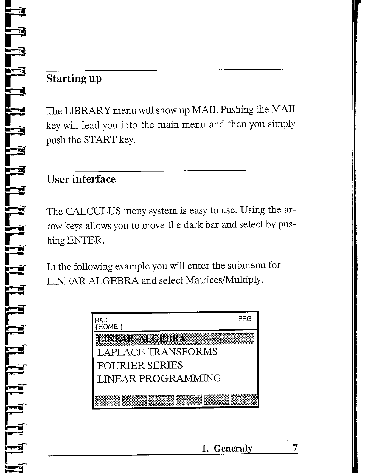
The

LIBRARY menu will

show

up

MAIL Pushing

the

MAJI

key

will lead

you

into

the

main,

menu

and

then

you

simply

push

the

START key.

User

interface

The

CALCULUS

meny

system

is

easy

to

use. Using

the ar-

row

keys

allows

you to

move

the

dark

bar and

select

by

pus-

hing

ENTER.

In the

following

example

you

will enter

the

submenu

for

LINEAR ALGEBRA

and

select Matrices/Multiply.

RAD
{HOME

}

PRG

LAPLACE TRANSFORMS
FOURIER

SERIES

LINEAR PROGRAMMING

\r^

-

1.

Generaly

RAD
{HOME

}

PRG

Linear equations

+

J&~

-k

t

Transformations
Eigenvalueproblems

*m*r-

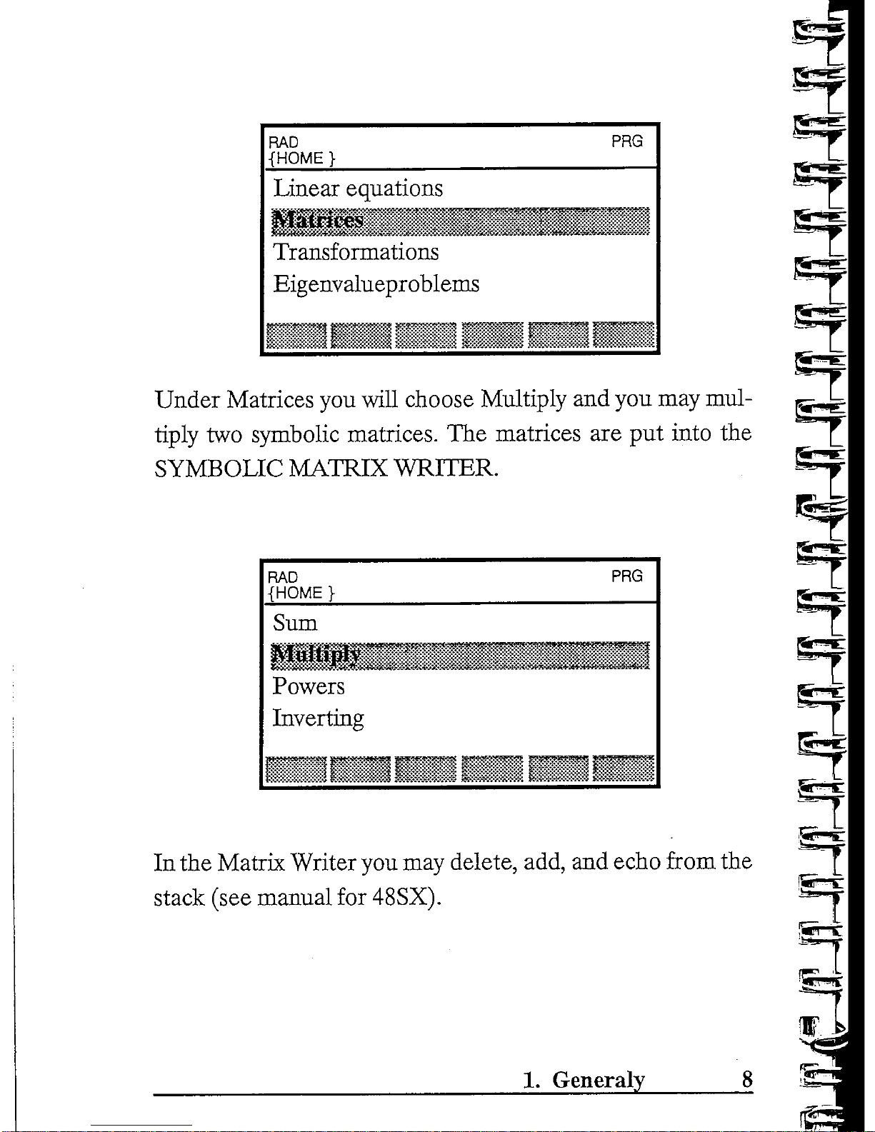
Under Matrices

you

will choose Multiply

and you may

mul-

tiply

two

symbolic matrices.

The

matrices

are put

into

the

SYMBOLIC MATRIX

WRITER.

RAD
{HOME}

PRG

Sum

Powers
Inverting

»*-<-»—»>«^

p«-v~«

1-

2*-

In the

Matrix Writer

you may

delete, add,

and

echo

from

the

stack

(see manual

for

48SX).

1.

Generaly

The

input Editor

If

you

select Linear equations under LINEAR ALGEBRA

you

will enter

the

editor

for

input (input screen).

RAD
{HOME

}

:PartAns

w

-"'•

sp"*r

, , ,JV.

»

PRG

Y/N:J

.}:

{123}

}:

{xyz}

Here

the

input data

can

be

modified

and

deleted

and

you can

move

around

by

using

the

arrow keys.

The

cursor

is

placed right behind

:PartAns

Y/N:

and

here

you

enter

Y if you

want intermediate results.

The

arrow

keys

are

used

to get

right behind

:B

{Bl...}:

and

here

you

enter

the

right

side vector

of the

system.

If

you

have done a mistake

you may

alter

your input

by

using

the

delete

keys

on the

calculator keyboard.

You

will

not be

able

to

continue before

the

data

are

correctly

put in.

1.

Generaly

In the

input screen there

is

often

information about

the

pro-

blem

you are

going

to

solve

(formulaes

etc).

Remember

the

' ' in

algebraics

and

separation

of

several data

on the

same

input

line

by

using blanks

(space).

Echoing

from the

stack

If

an

expression

or a

value laying

on the

stack

is

going

to be

used, then

the

EDrT/tSTK/ECHO/ENTER

sequence will

load

data into

the

input screen.

Be

sure

to

place

the

cursor

correctly

Calculation

finished

When a calculation

is finished

CALCULUS will

either

show

up

intermediate results

by

using

the

VIEW

routine (intrinsic

MAII)

or

return directly

to the

menu.

In the

last case

you

will

need

to use

the

->STKkey

to see the

result laying

on the

stack.

Moving

up and

down

in the

menu

You

can

move downwards

in the

menu system

by

scrolling

the

dark

bar and

pressing

ENTER.

If you

need

to

move

up-

wards

the

UPDIR

key

will

help.

At any

time

you may

HALT

CALCULUS

and use the

calculator independent

of

CAL-

CULUS

by

pressing

the

-^STK

key.

CONT

will

get you

back

to

the

menu system.

1.

Generaly

10

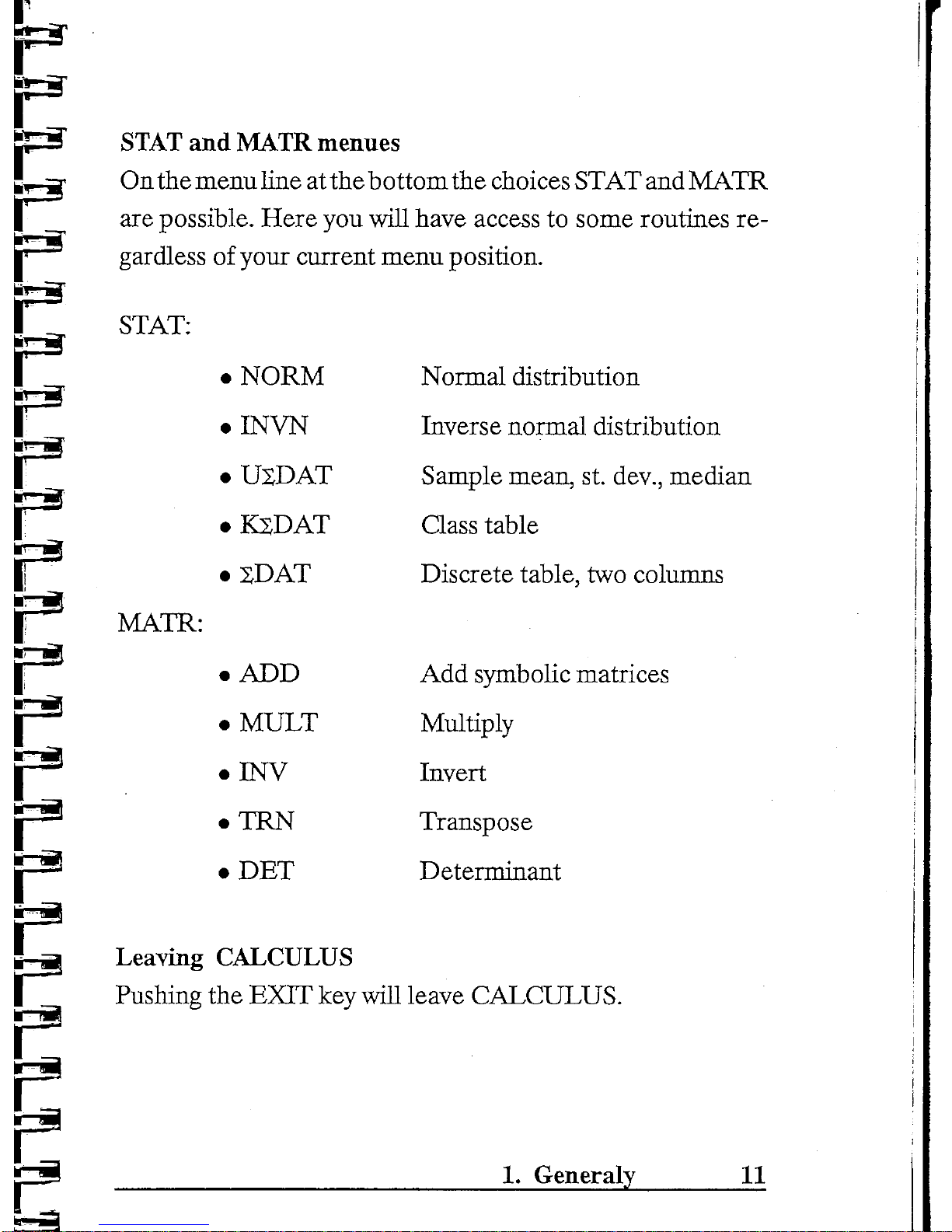
STAT

and

MATR

menues

On

the

menu

line

at

the

bottom

the

choices

STAT

and

MATR

are

possible.

Here

you

will have access

to

some routines

re-

gardless

of

your current menu position.

STAT:

MATR:

•

NORM Normal distribution

•

INVN

Inverse normal distribution

•

USD

AT

Sample mean,

st.

dev.,

median

•

KSDAT

Class table

•

SDAT

Discrete table,

two

columns

• ADD Add

symbolic matrices

•

MULT Multiply

•

INV

Invert

•

TRN

Transpose

• DET

Determinant

Leaving

CALCULUS

Pushing

the

EXIT

key

will leave

CALCULUS.

1.

Generaly

11

Intermediate

results

In the

input screen

you may

choose

PartAns

Y/N.

Choosing

N

the

result

will

be

laying

on the

stack

and you

have

to use

-^STK

to see the

answer. Choosing

Y,

different

pages

of in-

termediate results will

show

up or

more than

one

result

is

lay-

ing

on the

stack.

The

degree

of

details

in the

partial answers

is

somewhat dif-

ferent,

but

some

of the

results covers "the whole answer".

In

E:'"^

"~

~-~""

every

case this will give

the

user a good help.

Different

parts

of an

answer

may be

found

on

different

pages

and

the

page number

can bee

seen (use arrow up/down).

When PartAns Y(es)

is

chosen

all

numbers will show

up

with

two

figures

behind comma.

If a

more accurate answer

is ne-

cessary,

you

will have

to

look

on the

stack

and

perhaps

use

the N FIX

option.

s=^-r

Flag

status

and CST

menu

The flag

status

and CST

menu

you

have before going into

CALCULUS will

be

restored when

you

leave

by

pushing

EXIT.

3

5

s=*

1.

Generaly

12

Linear algebra

The

subject linear algebra covers

linear

eqautions

with solu-

tion also

for

singular systems, matrix manipulation (symbo-

lic), eigenvalue problems included systems

of

linear

differential

equations,

linear

transformations

in two and

three dimensions

and

vector spaces.

Linear equations (Gauss method)

Linear equations with symbolic parameters

are

handled.

The

equations have

to be

ordered

to

reckognize

the

coefficient

matrix

and the

right

side.

The

equations

are

given

in the

form:

E^-sr

r~

Br-g

A is the

coefficient

matrix

, X a

column vector

for the un-

I

j

knowns

and

B the

right

side column vector. Symbolic

coeffi-

|

cients

are

possible.

2.

Linear algebra _ 13

If

Det(A) = 0

(determinant)

the

system will

be

singular (self

contradictory

or

indefinite).

This

is

stated

as

"Self

contradic-

tory"

or the

solution will given

in

terms

of one ore

more

of

the

unknowns (indefinite). Example:

{x,y,z} = {x,2*x-l,x-4}

The

value

of x is

arbitrary

so

there

is an

infinite number

of

solutions.

If

the

system

is

underdetermined

(too

few

equations),

the so-

JS^g

lution

will b e

given

in the

idefinite

form.

If the

system

is

over-

[__

determined (too many equations)

the

solution will

be

given

in the

indefinite

form

if the

equations

are

lineary dependent

or as

"Self

contradictory"

if

they

are

lineary independent.

L

The

solution algorithm

is the

Gauss elimination.

If

PartAns

Y(es)

is

selected,

the

different stages

in the

process will

be

given

as

matrices

on the

stack which

may be

viewed

by

using

the

MATW

option (LIBRARY).

The

coefficient

matrix

and

the right

side vector

are

assembled

in one

matrix

(B is the

^;_^

rightmost

column).

^-

L

2.

Linear algebra

14

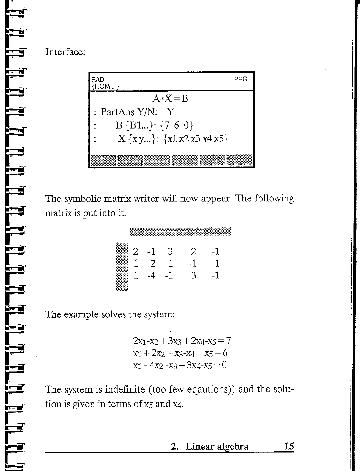
Interface:

RAD

{HOME}

PRG

A*X

= B

:

PartAns

Y/N:

Y

:

B{B1...}:

{7

6 0}

...}:

{xlx2x3x4x5}

V,

f,

m

j,,.>™»

„,,«

'

.-

H

tt

The

symbolic matrix writer will

now

appear.

The

following

matrix

is put

into

it:

'

2

i

i

1

1

5

-1

2

-4

3

1

-1

2

-1
3

-1
1

-1

The

example solves

the

system:

2xi-X2

+ 3x3 + 2x4-xs = 7

xi + 2x2+X3-X4+xs

= 6

xi

- 4x2

-xs + 3x4-xs

= 0

The

system

is

indefinite (too

few

eqautions))

and the

solu-

tion

is

given

in

terms

of

xs

and

X4.

2.

Linear algebra

15

Matrix

calculations

Some

operations

on

symbolic matrices

are

done (not cove-

gjr

red

by the

48SX intrinsic

functions).

The

matrices

are

put

into

the

SYMBOLIC MATRIX

WRITER

and the

matrix

is put

*"**

on

the

stack

by

pushing

ENTER.

Addition

Both

matices

are put

into

the

matrix writer

and

added.

An er-

ror

message

is

given

for

wrong dimension.

Multiplication

Both

matrices

are put

into

the

matrix writer

and

multiplied.

An

error message

is

given

for

wrong dimensions.

The

first

matrix

has to

have

the

same number

of

columns

as the

sec-

ond

has

rows.

Be

aware

of the

order

of the

matrices.

Inverting

The

mark

is put

into

the

matrix writer

and

inverted.

An er-

^

ror

message

is

given

if its not

quadratic.

Determinant

^T

The

determinant

of a

symbolic matrix

is

calculated.

The ma-

~~

trix

is put

into

the

matrix writer.

An

error message

is

given

if

its

not

quadratic.

2.

Linear algebra

16

Rank

of a

matrix

The

rank

of a

mark

is

calculated. This

routine

may be

used

for

testing

linear

independency

of

rowvectors.

The

routine

makes

the

matrix upper

traingular

and

PartAns Y gives

the

different

stages

of the

process.

Trace

The

trace

of a

square matrix

is

calculated.

An

error message

is

given

if the

matrix

is not

quadratic.

Orthogonal matrix

This routine

is

testing whether

the

matrix

is

orthogonal i.e.

the

inverse

is

equal

to the

transpose.

An

error message

is gi-

ven for

wrong dimension (must

be

quadratic).

The

answer

is

logic

0 or 1. May be

used

to

investigate

if

rowvectors

are

ort-

hogonal

i.e.

is an

orthogonal basis

of a

vector space.

Transpose

matrix

The

transpose

of a

symbolic matrix

is

calculated.

Symmetric

Investigates

whether a matrix

is

symmetric

or

not. Logic

0 or

1.

2.

Linear algebra

17

Linear transformations

Linear transformations include coordinate transformations

in

the

plane

and in the

three dimensional space.

The

trans-

formations

are

rotation, translation

and

scaling.

The

point

to

be

transformed

is

given relative a rectangular coordinate sys-

tem.

Mixed

transformations

(concatinating)

is

possible.

The

order

of

the

transformations

is

important

if

rotation

is one of the

them.

2

gir-TC

2 D

transformations (two

dimensions)

Rotation

The

rotation angle must

be

given

in

degrees'

and the

transfor-

med

point

is

given

as

components

of a

list

(to

allow symbols).

The

rotation

is

counterclockwise

for

positive angles about

an

arbitrary

point.

Bf

3

a

„

2.

Linear algebra

18

50

0

2'Q

4-0

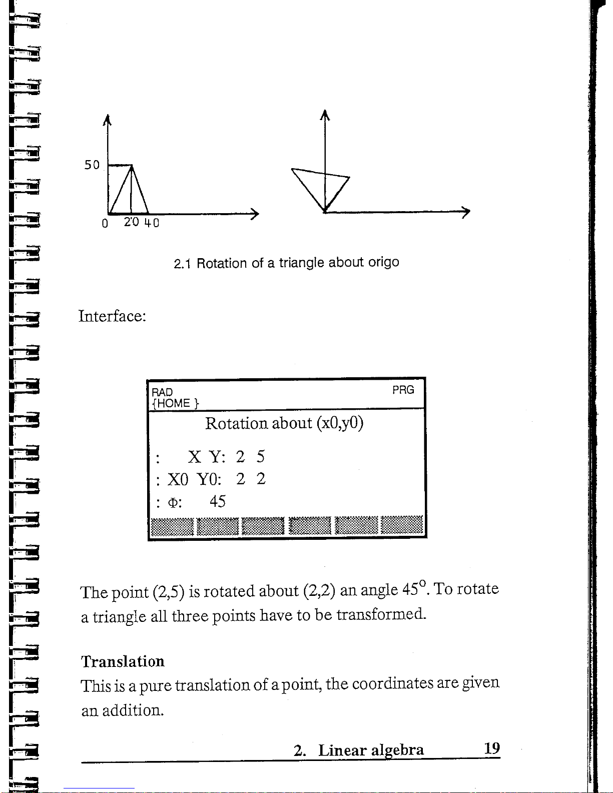
2.1

Rotation

of a

triangle

about

origo

Interface:

RAD

{HOME

}

PRG

Rotation

about

(xO,yO)

X

Y: 2 5

XO

YO: 2 2

$:

45

T5^ra.*\

]£KO*.

•* « -^

±

*

>

*.

*

J

*^ ^ > A

*

The

point

(2,5)

is

rotated about

(2,2)

an

angle

45°.

To

rotate

a

triangle

all

three points have

to be

transformed.

Translation

*E15?

This

is a

pure translation

of a

point,

the

coordinates

are

given

r?

an

addition.

2.

Linear algebra

19

50"

60 -•

10 •

0

20 40

80

100

120

fi£

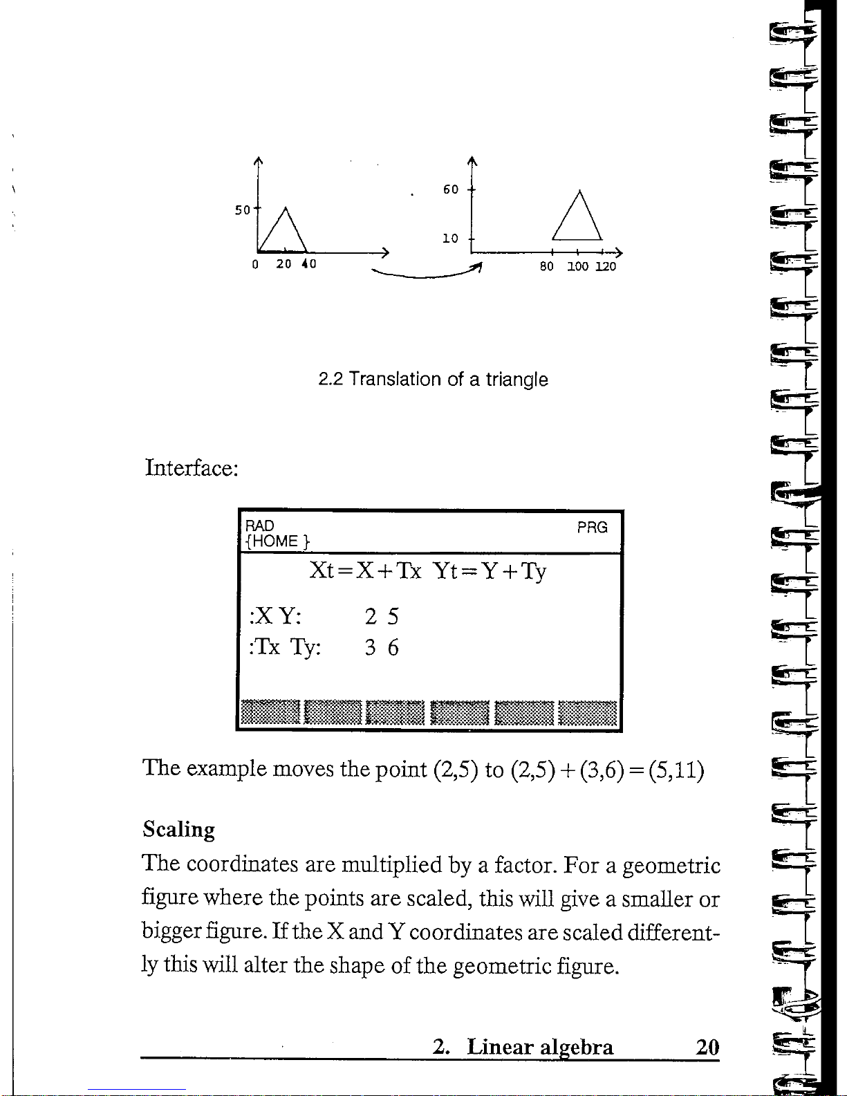
2.2

Translation

of a

triangle

Interface:

RAD
{HOME}

Xt

=

:XY:
:Tx Ty:

rrnrr

PRG

X+Tx

Yt = Y + Ty

2

5

3 6

inrir^cTi;—

i

The

example moves

the

point (2,5)

to

(2,5) + (3,6) = (5,11)

Scaling

The

coordinates

are

multiplied

by a

factor.

For a

geometric

figure

where

the

points

are

scaled, this will give a smaller

or

bigger

figure.

If the X and Y

coordinates

are

scaled different-

ly

this

will

alter

the

shape

of the

geometric

figure.

3
ff

»

2.

Linear algebra

20

r

F

50

A

100

-^

0

40

120

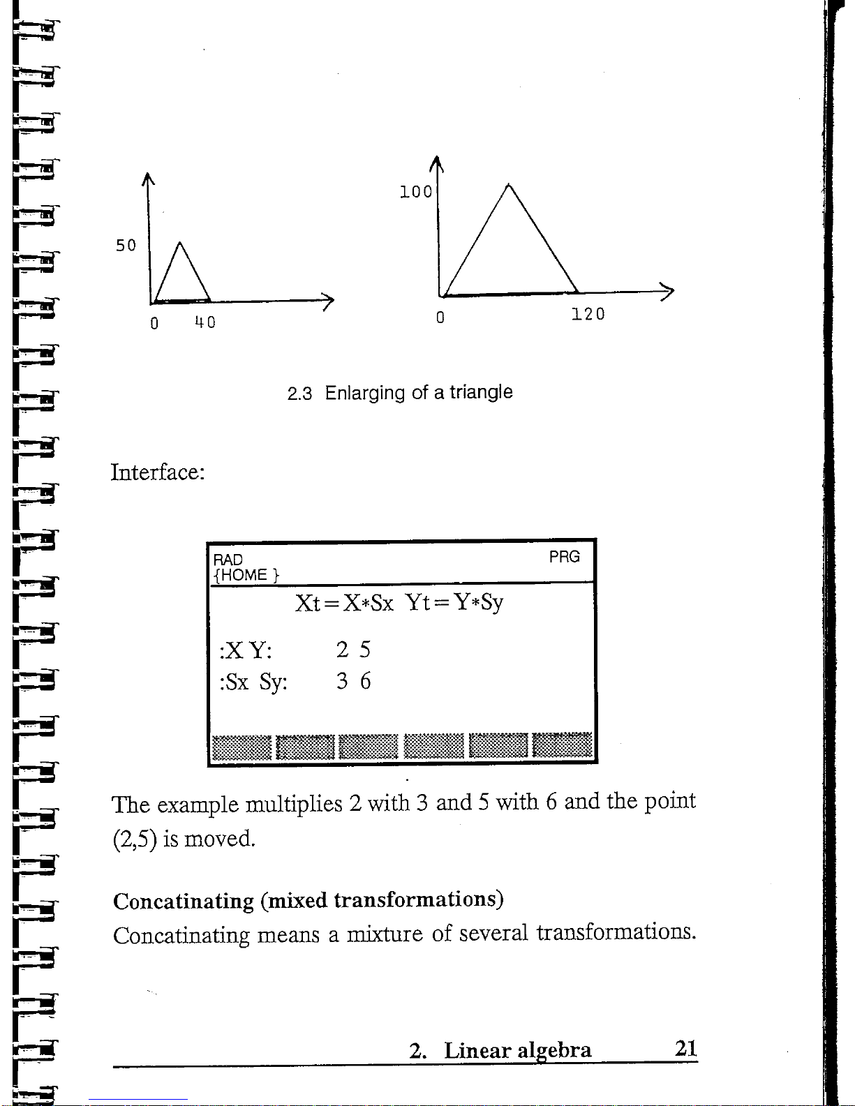
2.3

Enlarging

of a

triangle

Interface:

RAD
{HOME

}

PRO

:XY:
:Sx Sy:

; = X*Sx

Yt =

'

2

5

3 6

,_,^

,1*

--

The

example multiplies 2 with

3 and 5

with

6 and the

point

(2,5)

is

moved.

Concatinating (mixed transformations)

Concatinating means a mixture

of

several transformations.

2.

Linear algebra

21

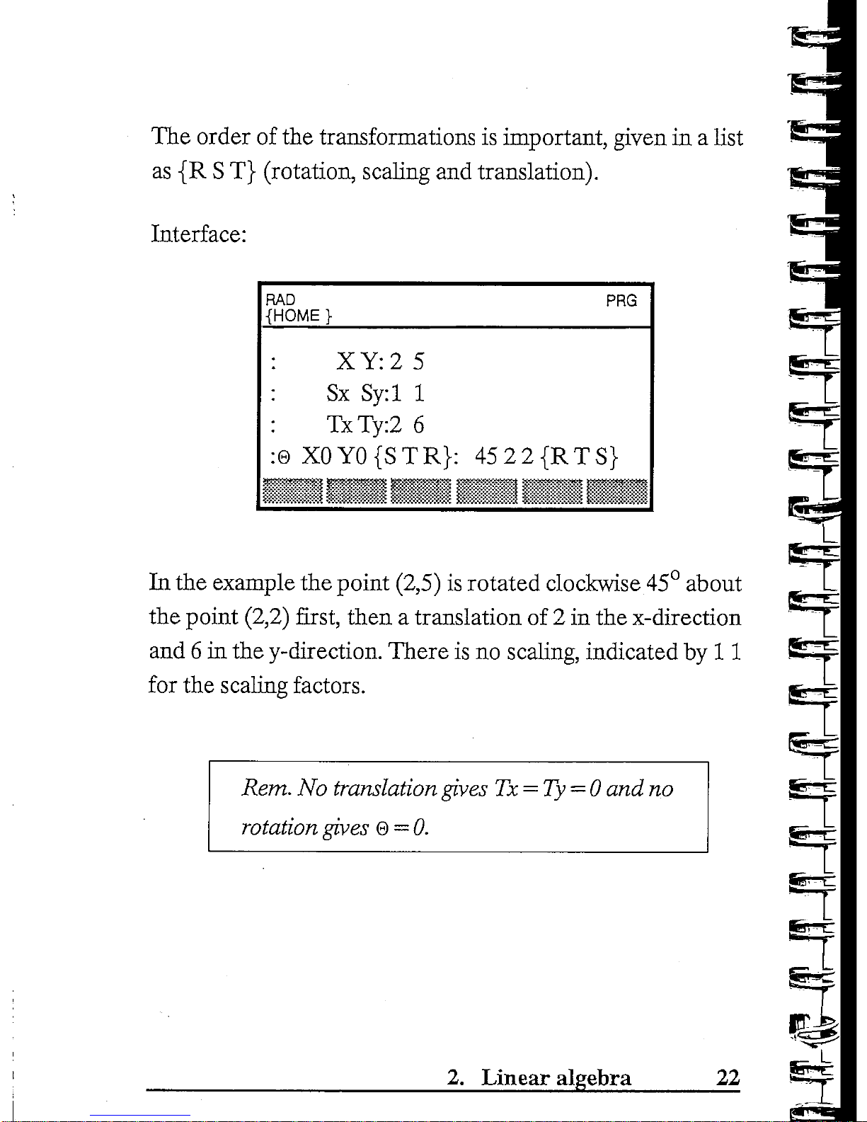
The

order

of the

transformations

is

important, given

in a

list

as

{R S T}

(rotation,

scaling

and

translation).

Interface:

RAD
{HOME

}

PRG

:

XY:25

: Sx

Sy:l

1

:

TxTy:2

6

:0XOYO{STR}:

4522{RTS}

In the

example

the

point

(2,5)

is

rotated

clockwise

45°

about

the

point (2,2)

first,

then a translation

of 2 in the

x-direction

and

6 in the

y-direction.

There

is no

scaling, indicated

by

11

for

the

scaling

factors.

Rent.

No

translation gives

Tx =

Ty = 0 and no

rotation

gives

0 = 0.

Sa-

2.

Linear algebra

22

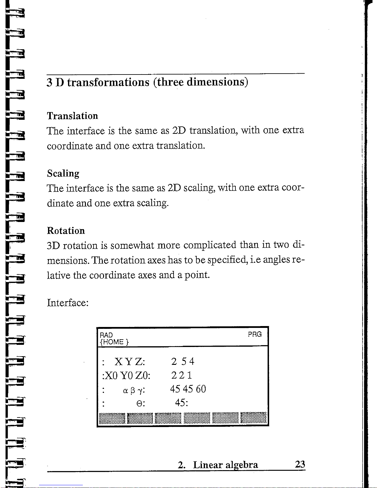
3 D

transformations

(three

dimensions)

Translation

The

interface

is the

same

as 2D

translation, with

one

extra

coordinate

and one

extra translation.

Scaling

The

interface

is the

same

as 2D

scaling, with

one

extra coor-

dinate

and one

extra scaling.

Rotation

3D

rotation

is

somewhat more complicated than

in two di-

mensions.

The

rotation axes

has to be

specified,

i.e

angles

re-

lative

the

coordinate

axes

and a

point.

Interface:

RAD
{HOME

}

:

XYZ:

:XO

YO ZO:

:

ap-y:

: 0:

"

-v-^w**-*™

-

•••

*§•

PRG

2 54
221

45 45 60

45:

i

S

2.

Linear

algebra

23

The

example rotates

the

point (2,5,4) about

an

axes through

the

point

(2,2,1)

and

with angles

relative

the x-, y-, and

z-axes

equal

to

45°,

45° and

60°.

Concatinating

(mixed)

The

same interface

as in the 2D

case,

but the

rotation axes

now

has to be

specified.

Interface:

e:

s

gr

fe

RAD

{HOME

}

:

XYZ:

:XO YO ZO:
:Sx Sy Sz:
:TxTyTz:

PRG

2

54

221

346

252

RAD
{HOME

}

a p

7:

45 45 60

0{STR}:

45{RTS}

PRG

3

rt

2.

Linear algebra

24

In the

example

the

point (2,5,4)

is

rotated about

the

given

axes

and

then

the

specified translation

and

scaling

is

carried

out.

Eigenvalueproblems

Here

you may

find

the

eigenvalues

and the

eigenvectors

of a

matrix,

diagonalize a matrix

and

solve a system

of

linear dif-

ferential

equations.

Eigenvalues

The

eigenvalues

of a

matrix

are

determined

by the

equation

A*X = x*X,

where

A is the

matrix

and X a

column vector (ei-

genvector),

x.

is

called

the

eigenvalue.

Interface:

RAD
{HOME

}

Det(A-x*I)

= 0

rPartAns

Y/N:

Y

PRG

"WJ-J

|f?«SS»«!yS»

l#,i

->,

2.

Linear algebra

25

Now

the

matrix

has to be

specified,

and you may put it

into

the

symbolic matrix writer:

466

1 3 2

-1 -5 -2

The

example

finds

the

eigenvalues

of the

matrix:

466

132

-1 -5 -2

,

L

The

matrix

has an

eigenvalue with multiplicity 2 (x. = 2).

Eigenvectors

A

matrix

has

infinite

many

eigenvectors because

the

system

of

equations

that

determines

the

vectors

are

indefinite.

The

eigenvectors

are

given

in

terms

of

arbitrary parameters. A set

of

eigenvectors will

normaly

be

linear

independent even

if

the

eigenvalues have multiplicity greater than

1. But

this

is

not

always

the

case.

fcr

2.

Linear algebra

26

•n

Interface:

RAD
{HOME}

PRG

Finds

X

: x: 2

:PartAnsY/N:

Y

The

matrix

now has to be put

into

the

matrix writer.

We use

the

same matrix

as in the

determination

of

eigenvalues.

By

choosing

PartAns

Y the

indefinite system

of

equations that

determines

the

eigenvectors will

be

given.

We see

that

only

two

of

the

eigenvectors

are

lineary

independent (only

one ar-

bitrary

parameter

c).

Diagonalization

For a

matrix

A we can

write:

Here

K is a

matrix composed

of the

eigenvectors

of A

which

have

to be

lineary independent.

D is a

diagonal matrix with

the

eigenvalues

on the

diagonal.

If the

eigenvectors

are

2.

Linear algebra

27

lineary dependent

(as in the

example

of

eigenvectors), then

|£

the

matrix cannot

be

diagonalized

(not

diagonalizable).

^,

Interface:

The

matrix

has to be put

into

the

matrix writer:

-455

-565

-556

The

output

is the

matrices K and

D.

The

matrix

K may be

found

by

inverting

K.

.Rera.

If

intermediate

results

are

wanted,

you

may

look

at the

problems

of finding

eigenva-

lues

and

eigenvectors

separately.

£•—

r

g*

System

of

differential

equations

Here

a set of

linear, homogenous differential equations with

constant

coefficients

are

solved

by

using

the

method

of

dia-

^

-

gonalization.

—-

L

2.

Linear algebra

28

Interface:

RAD

{HOME

}

PRG

dX/dt=

A*X

:X = {x,y...}:

{XYZ}

: t: t

'',%

*r

*

*"jfv*'?ifTx"

-455

-565

-556

The

following

system

is

solved:

dx/dt

= -

dy/dt

= -5x +

6y

+ 5

The

output contains

the

constants

Cl,

C2

and C3 and the in-

dependent variable

is t.

2.

Linear algebra

29

Rem.

If

intermediate

results

are

wanted,

you

may

look

at the

problems

of finding

eigenva-

lues

and

eigenvectors

separately.

Under

Info

some information about

the

solving strategy

is gi-

ven.

Vector

spaces

A

vector space

is a

collection

of

vectors relative a basis whe-

re

certain operations

on

them

are

defined. A basis

is a set of

linear independent vectors

from

the

space.

In an

orthogonal

basis

the

vectors

are

mutualy

orthogonal

(inner

product

equals

zero).

Basis?

This

routine

examines whether

a set of

vectors

in the

space

is

linear independent.

The

vectors

are

put

into

the

matrix

wri-

ter as

rows

and the

output

is

logic

0 or 1.

2.

Linear algebra

30

Interface:

466
132

-1 -5 -2

The

example examines whether

the

vectors

in

RB

{4 6 6}, { 1

3 2} and

{-1

-5 -2} are

lineary

independent

and

then

form

a

basis

in

RS

(three

dimensional vector space).

Norm

Here

the

length

or

absolute value

is

calculated.

The

input

vector

is

{vi

V2

vs....}

and the

output

is a

number

or an

expres-

sion

if the

vector

is

symbolic.

Norming

A

vector

is

transformed into

an

unit

vector

e = V/NORM(V).V

=

Scalar

product (inner product)

The

scalar product

of two

vectors

is

calculated.

Symbolic

vec-

tors

are

possible.

Orthogonalization

An

orthogonal basis

is

calculated with

an

arbitrary basis

as a

starting

point using

the

Gram-Schmidt process.

_

2.

Linear algebra

_

31

Interface:

466

132

-1 -5 -2

The

basis

bl = [4 6 6], b2 =

[13

2] and b3 = [-1 -5 -2] is

given

in

RS.

The

basis

is not

orthogonal,

but the

routine

makes

it

orthogonal.

Rem.

Symbolic

vectors

are not

possible

Orthogonal?

The

routine

examines whether a matrix

is

orthogonal.

If the

row

vectors building

up the

matrix

form

an

orthogonal basis,

then

the

matrix

is

orthogonal.

Orthonorming

The

routine

is

norming

an

orthogonal basis.

Vector

in new

basis

^

U

Given a vector

VBI,

i.e. relative a basis

Bl. A new

vector

re-

I

lative a basis

B2 is

calculated.

2.

Linear algebra

32

Interface:

RAD
{HOME

}

Xbl-Xb2

:X

{xl...}:

{142}

PRG

123
312
225

•113

-412
'265

The

vector

{142}

relative

the

basis

{[12

3], [3 1

2],

[225]}

is

transformed

to the new

basis

2.

Linear algebra

33

Interface:

1 1 0

0

1 1

1 0 1

2.

Linear algebra

34

A

matrix defines a linear

transformation

in a

vector

sp

ace

re-

tp

lative

the

"natural" basis. This routine calculates

a new

trans-

formation

matrix

relative

a new

basis.

The

"natural" basis

is

{[100],[010],[001]}inR3.

£

111

Oil

**-

001 frr-

The

transformation

matrix

{{110}{011}{101}}in

natu-

*""*•

ral

basis defines

the

transformation:

§E

L(X1,X2,X3) = (XI + X2,X2 + X3,X3 + Xl)

|

&

The

example calculates

the new

transformation matrix

rela-

tive basis

{[111],[0

11],[0 0 1]}.

Symbolic elements

are

pos-

sible

in the

matrices.

5-53

S-H

n

1-3

r:

•—a

e

2.

Linear algebra

35

Laplace

transforms

u(t-a):

IF t a <

THEN 0 ELSE

IF t a >

then

1 END END

Laplace transforms

are

used

for

solving differential equa-

tions

and

can, contrary

to

other methods, deal with functions

f(t)

that

are

discontinous

in the

equation

a*y"

+b*y' + c*y=f(t)

*e^~

£

Discontinous f(t)

may be

composed

by

using

the

Unit Step

function

u(t-a) defined

as:

~

This

function

is not

implemented

in

CALCULUS

in

other

ways

than

as a

symbol,

and the

user

has to

make a program

~

<--

to

define

it

for

evaluation.

"

I

3

3

3.

Laplace

transforms _ 36

Laplace

transform

The

Laplace transform

of the

following functions

may be fo-

und:

• f (t) = Sin(a*t), a arbitrary

•

f(t) = Cos(a*t), a arbitrary

•

g(t)

=f(t)*ea , a

arbitrary

•

g(t)=f(t)*u(t-a),a>0

•

g(t) = f(t)*u(t-a)*ebt,

a>0 b arbitrary

•

h(t)=g(t)*t

•

Linear combinations

of

theese

functions

Interface:

RAD

{HOME}

PRG

F(s)=L(f(t))

:t

s: t s

:f(t):t^2*u(t-l)

The

example calculates

the

Laplace transform

of

=

t~2*u(t-l).

3.

Laplace transforms

37

.

,/f

CALCULUS cannot

find the

Lapla-

ce

transform

an

error

message

is

given (the

transform

does

not

exist

or its not

implemen-

ted)

Inverse

Laplace transform:

The

inverse transform

is

calculated.

The

types

of

functions

which

can be

inverted

are the

transforms

of the

functions lis-

ted on

page

37.

Interface:

n

RAD
{HOME

}

PRG

f(t)=InvL(F(s))

:s

t: s t

The

example

calculates

the

inverse

transform

of

3.

Laplace transforms

38

Inverse L Partial fractions

If

the

denominator

of

F(s)

is of

second degree

and may be

factorized

in

first

degree

factors,

or of a

higher degree than

2,

the

denominator

has to be

split into partial fractions.

Intermediate results (Partial Answers)

is

possible

to

show

the

splitting

into partial

fractions.

Rem.

If

the

transformation

does

not

exist

the

error

message

"does

not

exist"

is

given.

If

the

expressionis

too

complicatedthemessage

"not

rational"

may

appear.

The

expression

may

then

be

split

up.

3.

Laplace transforms

39

Interface:

fet

RAD

{HOME

}

: t s

:PartAns

n i ?"*

*""*"'<

F(s)=P(s)/Q(s)

InvL(F(s))=f(t)

: t s

Y/N:Y

V*

J« I %

*

PRG

•^

^

RAD

{HOME}

Input cont

:Numerator

P:

:Exp(-ir*s)'

:Denominator

Q:

's ^ 2-1'

PRG

v^

*•

In the

example F(s) = &"***/(s

-1) is

split into partial fractions

and

then

transformed.

The

shift

e"778

will

be

taken care

of

be-

fore

the

splitting into partial fractions.

3.

Laplace transforms

40

5

S£"-c

S

Jjjp-C

IB

e*

Differential

equations (initial value problem)

Laplace transforms

are

suitable

for

solving initial value pro-

blems,

in

particular when

the

"right hand side function"

is

discontinous.

The

answer

is

given

in the

form

Y(s)

=P(s)/Q(s)/R(s)

which

has

to be

transformed into

P(s)/((Q(s)*R(s)))

before

the ro-

utine

for

partial fractions

is

used

to

solve

the

problem.

Interface:

RAD
{HOME

}

PRG

ay"

+ by' +

cy = f(t)

y(0)=yOy'(0)=DyO

:abcyODyO

:

13201

:

f(t)

t:

'SIN(t)'

t

The

equation

y" + 3y'4-2y = Sin(t)

with initial conditions

y(0)

= 0 and

y'

(0) = 1 is

transformed.

3.

Laplace transforms

41

Probability

In

this chapter

of

probabihty

theory

we

will look

at

unlike

di-

screte

probability distributions

in

addition

to the

normal dis-

tribution which

is

continous.

For the

discrete distributions

both

the

cummulative

probability

and the

point probability

may

be

calculated.

For the

discrete

distributions

and in

connection with

pure

combinatorial calculations,

we

have

distinquished

between

with

and

without replacement.

e=

B:

5:
^

3

Rem.

Probabilities

must

be

less

then

or

equal

to

1 and

greater

than

or

equal

to 0.

•UT

L

4.

Probability

42

WBT

't_

Without

replacement

Without

replacemnet

means that

we

dont

put the

drawn ele-

ment back again.

Combinations,

not

ordered

This routine calculates

the

number

of

possibilities

to

draw

k

elements

of

total n without replacement

and

without regard

to

order.

Interface:

RAD

{HOME

}

N

:n

k:

PRG

Draw

k of n

F = n!/((n-k)!*k!)

15

3

^_^_^

.

^

The

example calculates

the

number

og

possibilities

to

draw

3

elements

form

total

15

elements without regard

to

order.

4.

Probability

43

Combinations, ordered

If

the

order

is

important

you

will have

to use

this routine.

The

same elements

in

different

orders will

then

be to

separate

events.

Interface:

RAD

{HOME

}

:n

k:

Draw

k of n

ordered

N =

n!/(n-k)!

15

3

*.J*%*^**;*i

JJ'X^-tWw!''^«^J

•&.*

•S^^'!'

•••*

W*^**^*1

*

if

i1

/.,*>»».

^

l*« K si

PRG

^-")

-i-

-X

•***•

I"

e
&

&

e

The

example calculates

the

number

of

combinations when

drawing 3 elements

from

15

with regard

to

order.

Hypergeometric

distribution

Here

the

probability

of

drawing exactly k X'es

from a popu-

lation

of n

when a elements

are

drawn

at a

time without

re-

placement

is

calculated.

The

probability

for

the X to b e

drawn

is

p.

3

Ew-c

gw-

E:

4.

Probability

44

Interface:

RAD
{HOME

}

: n a:
:pk:

—

::i

PRG

kX'es

ofn

drawaP(X)=p

20

8

0.6

3

VT;*:.'

Vi

~:x:

:.}&::

The

probability that 3 elements have

the

mark X when dra-

wing 8 elements

of

total

20 is

calculated.

The

probability

of

X

to

occur

is

0.6.

If k > a or p > 1 the

probability

is 0.

The

example

may be

"drawing" individuals

from a population

of

20

where

12 is

women

(p =

12/20 = 0.6).

The

probability

that

of 8

"drawn"

individuals

3 is

women

is

calculated.

Hypergeometric

distribution

function

The

cummulativeprobability

is

calculated, i.e.

the

probability

that maximum k elements

are

drawn. This

is the sum of the

probabilities

of k =

0,k = l,k = 2 and k = 3.

4.

Probability

45

Interface:

RAD
{HOME

}

:

n a:

:pk:

maxkX'es

of n

drawaP(X)=p

20

8

0.6

3

PRG

11

- .

The

example calculates

the

probability that 3 elements

is

drawn

with

the

mark

X (p =

0.6)

from a total

of 20 by

drawing

4

at a

time

or 1 by 1

without replacement.

With

replacement

Here

the

elements

are

replaced

by

drawing

so

that

the

prob-

ability

is the

same every time

an

element

is

drawn (uncondi-

tional drawing).

Combinations,

unordered

This routine calculates

the

number

of

combinations

of

dra-

wing k elements

from n without replacement, without regard

to

order.

4.

Probability

46

Interface:

RAD
{HOME}

PRG

Draw

k of n

:n k:

15

3

Here

the

probability

of

drawing 3 elements

of

total

15 is

cal-

culated.

Order

is

indifferent.

Combinations,

ordered

If

the

order

is

critical, this routine

has to be

used.

The

same

elements

in

different

orders

are two

separate events.

Interface:

RAD
{HOME}

PRG

:n k:

Draw

k of n

ordered N = n ^

k

15

3

4.

Probability

47

The

example calculates

the

number

of

possibilities with

the

same figures

as in the

previous example,

but now

with regard

to

order.

Binomial

distribution

The

routine calculates

the

probability

of

drawing exactly

k

elements with

the

mark

X of

total

n,

where

the

probability

of

X

itself

is p.

Independent trials (with replacement).

Interface:

RAD
{HOME

}

:np:
: k:

ofrrsf*

PRG

kX'es

of n

P(X)=p

10 0.6
3

The

probability

of

drawing 3 elements with

the

mark X when

X

has the

probability

of 0.6 is

calculated.

The

number

of in-

dependent trials

is 10. p > 1

gives

an

error message.

The

example

may be the

production

of

glasses where

the

probability

of

first

assortment

is

0.6.

If 20

glasses

are

produ-

4.

Probability

48

ced,

the

example calculates

the

probability that 3 glasses

are

first

assortment.

Binomial

distribution function

The

cummulative

probability

is

calculated,

i.e.

the sum

of

the

probabilities

for k =

0,

k=l, k = 2 andk=3

if k = 3.

Interface:

RAD

{HOME

}

PRG

maxkX'es

of n

P(X)=p

10

0.6

3

-.

The

example calculates

the

probability that maximum 3 ele-

ments

have

the

mark

X (p =

0.6)

in 10

independent trials.

Negative

binomial distribution

This distribution gives

the

probability

of k

failures

before

the

rth

success

in a

series

of

independent trials each

of

which

the

probability

of

success

is p.

4.

Probability

49

Interface:

RAD

{HOME}

PRG

k not

X'es before

XrthtimeP(X)=p

r p: 10

0.25

k:

15

f

^-

•% „ %

•*s~*5«*

z-"^

r*

The

probability

of 15

failures before

the

10th success when

the

probability

of

success

is

0.25

is

calculated.

The

example

may be the

drawing

of

cards

and the

calculation

of

the

probability

of

drawing

15

cards that

are not

clubs

be-

fore

the

10th club.

S

Negative

binomial distribution function

This routine calculates

probability

of

maximum k failures

be-

fore

the

rth

success.

4.

Probability

50

Interface:

RAD
{HOME

}

PRG

max

k not

X'es before

X

rth

time

P(X)=p

: r p: 5 0.4
: k: 4

The

probability

of

maximum 4 failures

before

the 5th

success

is

calculated. Probability

of

success

is

0.4.

The

example

may be the

drawing

of

balls

from a hat

that con-

tains

40%

white balls.

The

probability

of

finding

5 not

white

balls before drawing maximum 4 white balls

is

calculated.

Pascal

distribution

The

probability

of the rth

success

in kth

trial

in a

series

of

in-

dependent trials

is

calculated.

4.

Probability

51

Interface:

L

RAD
{HOME}

PRG

r

p:

k:

X

rth

time

kth

trial

P(X)=p

5 0.5

8

The

probability

of

finding

the

mark

X 5th

time

in the 8th

tri-

al

is

calculated.

_

L

Rem.

The

geometric

distribution

is a

special

case

with

r=l.

a

fee

Pascal distribution function

The

probability

of the rth

success

in

maximum k trials

is

cal-

culated.

The

probability

of

success

is p.

4.

Probability

52

Interface:

RAD

{HOME}

PRG

: r p:
: k:

X

rth

time

max k

trials

P(X)=p

5 0.5

8

The

example calculates

the

probability

of

finding

the

mark

X

the 5th

time

in

maximum 8 trials (Tossing a fair

coin

we

find

the

probability

of

finding

the 5th

head

in

maximum 8 trials).

Normal distribution

This

is a

continous distribution

and

only

cummulative

prob-

abilities

are

calculated.

4.

Probability

53

Interface:

RAD

{HOME}

PRG

Normal distribution

param. ^ and

o-

gives

P(X<x)

JLCT:

0 1

x:

1

The

probability that a random variable

is

less than

or

equal

to

1 is

calculated.

The

mean

and the

standard deviation

is 0

and

1.

Rem.

P(a<x<b)=P(x<b)-P(x<a)

and

P(x>a)=l-P(x<a)

Poisson

distribution

£

The

Poisson distribution

is

used

as a

model when

we are in-

terested

in

events within intervals

of

time

or

other variables.

3

"T

4.

Probability

54

Interface:

RAD

{HOME}

PRG

Poisson distr.

mean

p,

and P(X = k)

:ak:

4 5

The

example calculates

the

probability that a random

varia-

ble X is

exactly 5 when

the

mean

is 4.

Poisson distribution function

Interface:

RAD
{HOME

}

PRG

Poisson distr.

meanjx

and

P(X<k)

:

45

4.

Probability

55

The

probability that

X is

less

then

or

equal

to 5 is

calculated,

the

mean

is 4.

Info

Here

information about probability

and

some distributions

is

given.

Binomial

coefficients

Binomial

coefficients

Bnk = n!/((n-k)!*k!)

are

calculated

from k = 0 to k =

n and put in a

list.

Interface:

RAD
{HOME

}

PRO

Binomial

coeff.

=

n!/((n-k)!*k!)

k = 0...n

The

example calculates {BnO

Bnl

Bn2

Bn3

Bn4

Bn5}.

4.

Probability

56

Statistics

We

will

focus

on

some statistical methods

and

description

of

samples. Within description

of

samples

we

will

use

discrete

tables

and

class

tables (discrete

and

class statistics).

You can

convert

from

class statistics

to

discrete statistics

by

using

the

mean value

of the

intervals

as the

discrete value.

Statistical methods

are

represented

by

confidence intervals

and

hypothesis testing

for

distributions.

The

"best"

fit for the

normal distribution uses

the

method

of

least squares.

The

normal distribution,

kjisquare

distribution

and

student-t distribution

are

included

and its

possible

to find

both

the

probability

and the

value

of the

random variable

for

given

probability.

5.

Statistics

57

Distributions

Normal

distribution

The

normal distribution gives

p(X<x)

for

given

x-value.

The

mean

\L

and

standard deviation

o-

have

to be

known.

Interface:

RAD
{HOME}

PRO

Normal

distribution

pararn. ^ and

o-

gives

P(X<x)

:^cr:

0 1

'

: x: 1

^ 3 ^

*"

'""'

*1 ^ *'"*'

*

V*

f**"^1**"11

^

'

>*

*%

A.

j. ^ i

P(X<

1) for n = 0 and

o-

= 1 is

calculated.

Inverse

normal distribution

The

routine

finds

the

value

of the

random variable x with

gi-

ven

probability

p, ^ and

o-

are

known.

5.

Statistics

58

Interface:

RAD

{HOME}

PRG

Normal

distribution

JLO-gives

x,P(X<x)=p

:^a:

0 1

: p: 0.6

>*v' > '«**'

•" < 5 " ''%.('<&•''

r*%***•*«

i

X1

f

'*•

S

The

value

of x

with

P(X

<x) = 0.6,

jj,

= 0 and a =

1 is

calcula-

ted.

Kjisquare

distribution

The

kjisquare

distribution

is

used

to find

confidence intervals

and

in

connection with

fitting a

distribution

to a

sample.

Interface:

RAD

{HOME

}

PRG

Kjisquare

distr.

degrees

of

freed.

KP(X<x)

: K x: 3 5.6

5.

Statistics

59

The

example calculates

P(X < 5.6) where

X is

kjisquaredistri-

buted with 3 degrees

of

freedom.

Inverse

kjisquare

The

value

of x for

given probability

is

calculated.

Interface:

*f

RAD
{HOME}

PRG

Kjisquare

distr.

degrees

of

freed.

KP(X<x)

=p

: K p: 3

0.85

3

The

example

calculates

the

value

of X so

that

P(X

<x) = 0.85

with 3 degrees

of

freedom.

Studen-t

distribution

This distribution

is

used

to find

confidence intervals

in

CAL-

CULUS.

"T

5.

Statistics

60

Interface:

RAD

{HOME

}

PRG

Student-t

distr.

degrees

of

freed.

KP(X<x)

: K x: 3 7.5

P(X<7.5)

with 3 degrees

of

freedom

is

calculated.

Inverse

student-t

This routine calculates

the

value

of the

random variable

x.

Interface:

RAD
{HOME}

PRG

Student-t distr.

degrees

of

freed.

KP(X<x)

=p

: K p: 3

0.85

The

value

of x is

calculated

so

that

P(X<x) = 0.85 with

3 de-

grees

of

freedom.

5;

Statistics

61

Confidence

intervals

Confidence

intervals

in

connection with

the

normal distribu-

tion

are

calculated

for the

mean , and

variance

o-

.

Rent.

Mean value

and

standard

deviation

for

a

sample

may be

calculated

under

this

menu.

Theese

values

may be

used

as

point

estimates

for

the

parameters

in the

distribution

function.

Confidence

interval

for the

mean

(x,

given value

of a.

For

known

a we may use the

normal

dsirribution

to

find

the

value

c so

that F(c) = P(x<

c) =

l/2(-/ + T)

with confidence

le-

vel

-/.

The

interval

is

given

in the

form

[a<

|x<b].

The

interval

is

calculated

from a sample