Hp COMPAQ PROLIANT 6500, COMPAQ PROLIANT 4000 Disk Subsystem Performance and Scalability

[September 1997]

.....................

............

.................

...

..............

....................

Prepared By Microsoft Windows NT Integration Team

Compaq Computer Corporation

C

ONTENTS

Disk Subsystem Overview

Disk-Related Performance Characteristics

Like Drive Scalability

Like Capacity Scalability

Disk Controller Scalability

Performance Measurement Tools

Preventing Data Loss while Maintaining Performance

Disk Subsystem Summary of Findings

ECG025.0997

17

19

24

27

28

29

W

.

Disk Subsystem Performance and

.

Scalability

.

In today's networking environments, the disk subsystem is a key element in determining

.

overall system performance. The goal of this paper is to provide informative test results

.

and performance-related information for various disk subsystems, to assist systems

.

engineers and network administrators in making decisions on disk subsystem installation,

.

optimization, and configuration.

.

3

4

This white paper also provides information on using Fault Tolerance to prevent data loss,

.

while maintaining system performance. Finally, this paper provides a section discussing

.

the advantages and disadvantages of RAID technology.

.

Help us improve our technical communication. Let us know what you think about the

.

technical information in this document. Your feedback is valuable and will help us structure

.

future communications. Please send your comments to: CompaqNT@compaq.com

.

1

HITE

APER

P

ECG025.0997

HITE PAPER

W

.

N

OTICE

.

The information in this publication is subject to change without notice.

.

C

OMPAQ COMPUTER CORPORATION SHALL NOT BE LIABLE FOR TECHNICAL

.

OR EDITORIAL ERRORS OR OMISSIONS CONTAINED HEREIN

.

INCIDENTAL OR CONSEQUENTIAL DAMAGES RESULTING FROM THE

.

FURNISHING

.

This publication does not constitute an endorsement of the product or products that were

.

tested. The configuration or configurations tested or described may or may not be the

.

only available solution. This test is not a determination of product quality or correctness,

.

nor does it ensure compliance with any federal, state or local requirements. Compaq

.

does not warrant products other than its own strictly as stated in Compaq product

.

warranties.

.

Product names mentioned herein may be trademarks and/or registered trademarks of

.

their respective companies.

.

Compaq, Contura, Deskpro, Fastart, Compaq Insight Manager, LTE, PageMarq,

.

Systempro, Systempro/LT, ProLiant, TwinTray, ROMPaq, LicensePaq, QVision, SLT,

.

ProLinea, SmartStart, NetFlex, DirectPlus, QuickFind, RemotePaq, BackPaq, TechPaq,

.

SpeedPaq, QuickBack, PaqFax, Presario, SilentCool, CompaqCare (design), Aero,

.

SmartStation, MiniStation, and PaqRap, registered United States Patent and Trademark

.

Office.

.

Netelligent, Armada, Cruiser, Concerto, QuickChoice, ProSignia, Systempro/XL, Net1,

.

LTE Elite, Vocalyst, PageMate, SoftPaq, FirstPaq, SolutionPaq, EasyPoint, EZ Help,

.

MaxLight, MultiLock, QuickBlank, QuickLock, UltraView, Innovate logo, Wonder Tools

.

logo in black/white and color, and Compaq PC Card Solution logo are trademarks and/or

.

service marks of Compaq Computer Corporation.

.

Other product names mentioned herein may be trademarks and/or registered trademarks

.

of their respective companies.

.

U.S.A.

.

Microsoft, Windows, Windows NT, Windows NT Server and Workstation, Microsoft SQL

.

Server for Windows NT are trademarks and/or registered trademarks of Microsoft

.

Corporation.

.

Disk Subsystem Performance and Scalability

.

First Edition (September 1997)

.

Document Number: ECG025.0997

.

2

(cont.)

,

PERFORMANCE, OR USE OF THIS MATERIAL

,

NOR FOR

.

ECG025.0997

HITE PAPER

W

.

ISK SUBSYSTEM OVERVIEW

D

.

Key components of the disk subsystem can play a major part of overall system

.

performance. Identifying potential bottlenecks within your disk subsystem is crucial. In

.

this white paper we identify and discuss in detail disk-related performance characteristics

.

that can help you understand how latency, average seek time, transfer rates and file

.

system or disk controller caching can affect your disk subsystem performance. Once we

.

discuss all of the disk measurement terms, we use those definitions to address

.

performance issues in each scalability section of this document. The different scalability

.

sections discussed are as follows:

.

• Like Drive (similar hard drive scalability)

.

• Like Capacity (similar drive capacity scalability)

.

• Disk Controller (multiple controller scalability)

.

This document provides disk subsystem recommendations, based on testing in the

.

Integration Test Lab of hardware and software products from Compaq and other vendors.

.

The test environment that Compaq selected might not be the same as your environment.

.

Because each environment has different and unique characteristics, our results might be

.

different than the results you obtain in your test environment.

.

Test Environment

.

The following table describes the test environment used for the disk subsystem

.

performance testing. This table displays both the one and two controller test

.

configurations that were used in the Compaq ProLiant 5000 during testing.

.

Environment Equipment Used

.

Server Hardware Platform Compaq ProLiant 5000

.

3

Memory 128 MB Processors (4) P6/200 MHz 512k secondary cache Network Interface Controllers (2) Dual 10/100TX PCI UTP Controller (4 network segments) Disk Controllers (1 or 2) SMART-2/P Controllers Disk Drives 2, 4, or 9 GB Fast-Wide SCSI-2 drives Number of Drives up to fourteen 2.1, 4.3, or 9.1 GB Fast-Wide SCSI-2 drives Boot Device (1) Fast-Wide SCSI-2 drive off the Embedded C875 controller

(cont.)

Table 1:

Disk Subsystem Testing Environment

ECG025.0997

HITE PAPER

W

.

Environment Equipment Used

.

Server Software Configuration Microsoft Windows NT Server version 4.0

.

D

.

Before beginning our discussion on disk subsystem performance, Table 2 lists the general

.

terms used in the industry to describe the performance characteristics of disk

.

performance. These general terms describe characteristics that can impact system

.

performance, so it is important to understand the meaning of each term and how it could

.

affect your system.

.

4

Service Pack 2 Compaq Support Software Diskette 1.20A Client Configuration Compaq Deskpro 575

NetBench 5.0 Test Configuration Disk Mix

Work Space 15 MB Ramp Up Time 10 seconds Ramp Down Time 10 seconds Test Duration 120 seconds Delay Time 0 seconds Think Time 0 seconds

ISK-RELATED PERFORMANCE CHARACTERISTICS

Terms Description

Seek Time The time it takes for the disk head to move across the disk to find a

Average Seek Time The average length of time required for the disk head to move to the

(cont.)

Table 1:

(cont.)

Disk Subsystem Testing Environment

Netelligent 10/100 TX PCI UTP Controller and MS-DOS

Table 2:

Disk Performance Measurement Terms

particular track on a disk.

track that holds the data you want. This average length of time will generally be the time it takes to seek half way across the disk.

ECG025.0997

HITE PAPER

W

.

Terms Description

.

Latency The time required for the disk to spin one complete revolution.

.

Average Latency The time required for the disk to spin half a revolution.

.

Average Access Time The average length of time it takes the disk to seek to the required

.

Transfer Rate The speed at which the bits are being transferred through an

.

Concurrency The number of I/O requests that can be processed simultaneously.

.

RPM (Revolutions Per Minute) The measurement of the rotational speed of a disk drive on a per

.

Table 2 lists the definitions of disk-related performance characteristics. Let’s now use

.

those definitions in the next several sections to address how adding drives to your system

.

can affect performance.

.

Seek Time and Average Seek Time

.

Seek time describes the time it takes for the disk head to move across the disk to find

.

data on another track. The track of data you want could be adjacent to your current track

.

or it could be the last track on the disk. Average seek time, however, is the average

.

amount of time it would take the disk head to move to the track that holds the data.

.

Generally, this average length of time will be the same amount of time it takes to seek half

.

way across the disk and is usually given in milliseconds.

.

5

(cont.)

Table 2:

(cont.)

Disk Performance Measurement Terms

track plus the amount of time it takes for the disk to spin the data under the head. Average Access Time equals Average Seek Time plus Latency.

interface from the disk to the computer.

minute basis.

ECG025.0997

HITE PAPER

W

.

One method to decrease seek time is to distribute data across multiple drives. For

.

instance, the initial configuration in Figure 1 shows a single disk containing data. The

.

new configuration reflects the data being striped across multiple disks. This method

.

reduces seek time because the data is spread evenly across two drives instead of one,

.

thus the disk head has less distance to travel. Furthermore, this method increases data

.

capacity because the two disks provide twice the space to store data.

.

6

Initial Configuration

New Configuration

Seek Time

Figure 1: Average Seek Time and Capacity

You can use this same concept and apply it to many different configurations. For example, if you currently have a two-disk configuration but you want to decrease the average seek time yet increase the disk capacity, you can configure a striped set of disks using four disks instead of two. This concept applies to any configuration (odd or even number of disks) as long as you are adding more drives to your stripe set.

(cont.)

Data

Seek Time

Data

Seek Time

Unused space Unused space

Unused space

Data

ECG025.0997

HITE PAPER

W

.

Average Latency

.

Manufacturers have built and continue to build hard disks that spin at designated rates. In

.

the early years of the personal computer (PC) industry, hard disks on the market could

.

spin at approximately 3600 RPMs. As the market demand for better system performance

.

increased, disk manufacturers responded by supplying faster spin rates for hard disks.

.

By producing faster spinning disks, manufacturers reduced the amount of overall access

.

time. Average latency directly correlates to the spin rate of the disk drive because it is, as

.

defined earlier in Table 2, the time required for the disk to spin half a revolution.

.

Therefore, this direct relationship in improving hard disk spin rates can contribute to better

.

system performance by reducing the average latency on a disk.

.

Manufacturers understand the need for better system performance and continue to

.

provide new and improved hard disks. With today’s hard disks spinning at 7200

.

revolutions per minute (RPMs) and the hard disks of tomorrow spinning at the rate of

.

10,000 RPMs, we can see that manufactures continue to address the issue of faster

.

performance. Table 3 provides a brief history on hard disks listing spin rates, disk

.

capacities available and approximate dates the disks were available to the market.

.

Disk Spin Rate Disk Capacity Approximate Date Used

.

3600 RPMs Up to 500 MB 1983 – 1991

.

4500 RPMs 500 MB – 4.3 GB 1991 – Present

.

5400 RPMs 500 MB – 6 GB 1992 – Present

.

7200 RPMs 1 GB – 9.1 GB 1993 - Present

.

10,000 RPMs 4.3 GB and 9.1 GB 1997 - Present

.

Now that we discusse d the direct relationship between disk spin rates and system

.

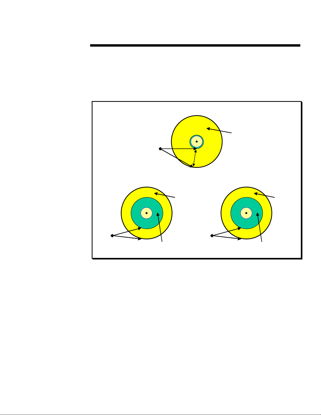
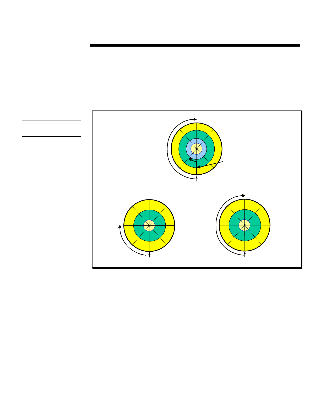
performance, let’s examine how drive scaling can affect latency. In Figure 2 - Example 1,

.

the initial configuration shows the disk has to spin halfway around before the disk head

.

can start to retrieve data from sector 5. In the new configuration, the disk has to spin half

.

the distance than before to retrieve the same data. Thus, the latency time has been cut

.

in half.

.

7

(cont.)

Table 3:

Hard Disk History

: Remember that the disks

Note

used in Figure 2 ar e ide n tic al in size and RAID configuration.

ECG025.0997

HITE PAPER

W

.

However, be aware that the average latency time might not always decrease when addi ng

.

more drives to your system. For example, in Figure 2 - Example 2, the new configuration

.

shows that the amount of time it takes to retrieve the data from sector B is actually longer

.

than the initial configuration. The reason for this is that the disk has to spin half way

.

around to read sector B. In the initial configuration the disk only had to spin one-eighth a

.

revolution to read the identical data. But, keep in mind that the initial configuration for

.

Example 2 required both seek time and latency time.

.

8

Initial Configuration

New Configuration

Example 1

Figure 2: Average Latency

Overall, these examples show us that in some configurations, as shown in our first example, drive scaling would be a definite performance advantage. However, in other configurations it is not clear if you receive a performance gain because of the components involved, such as the combination of average seek time and average latency time used in Figure 2 – Example 2.

When you combine these terms (average seek time and average latency time), you define another disk measurement called average access time, which is discussed in the upcoming section. From the information provided in this section, we know seek time plus latency (or average access time) is a key in determining if performance is truly enhanced in your system.

(cont.)

5

3

Example 1

A

7

1

G

Disk Head

4

D5E

3

C

B

2

H

A

1

Disk Head

C

Example 2

E

6

F

G

7

Example 2

8

B

8

6

4

2

Disk Head

D

F

H

ECG025.0997

HITE PAPER

W

.

Average Access Time

.

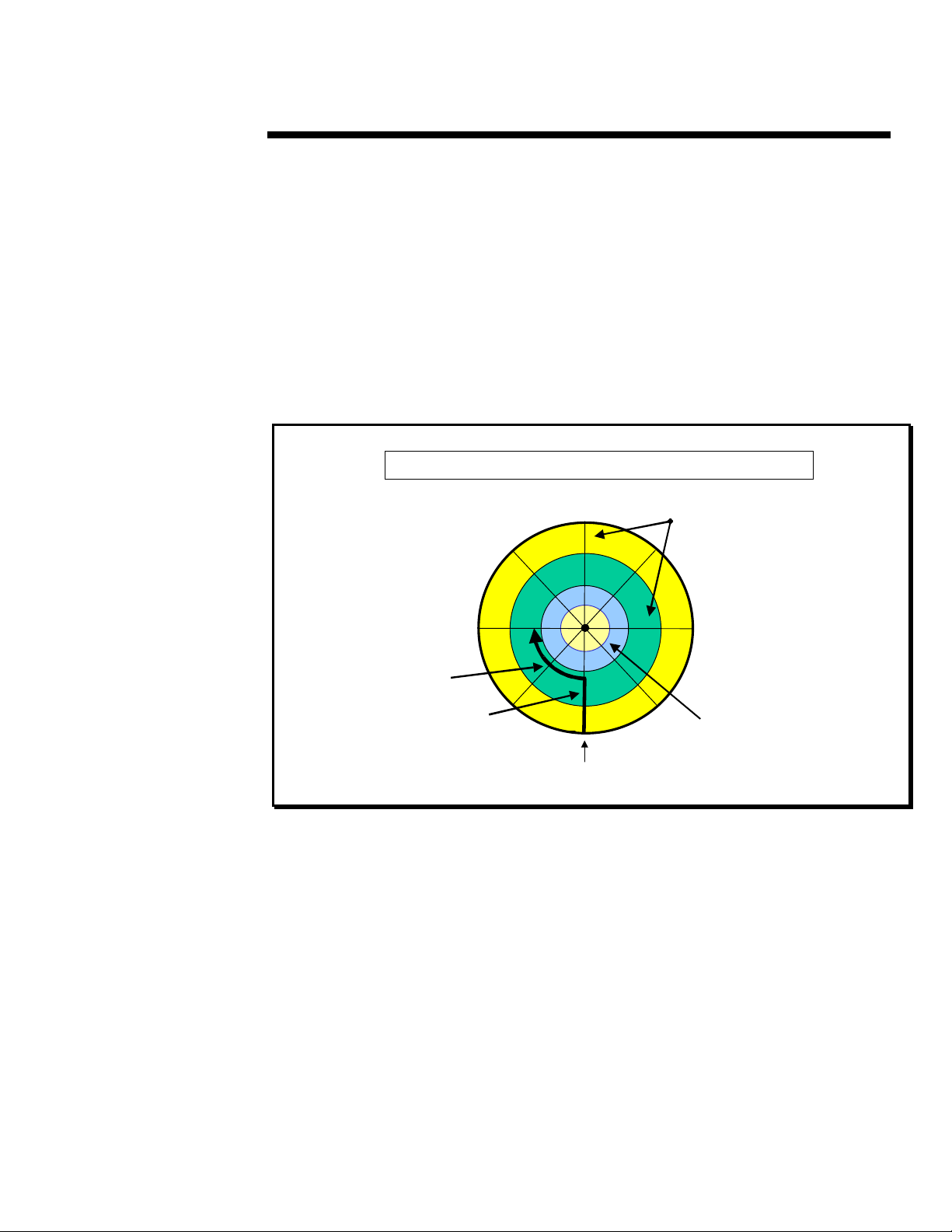
Average access time is simply described as average seek time plus latency. What this

.

equates to is the amount of time the disk has to seek to find the data plus the time it takes

.

for the disk to spin under the head. For example, Figure 3 contains a disk with two tracks

.

of data on it. Track 1 contains data sectors 1 – 8. Track 2 contains data sectors A – H.

.

Thus, in our example, the disk head has to move (or seek) from the current position (track

.

1, sector 1) to the track you want to read (track 2, sector C).

.

For the purpose of our illustration, Figure 3 displays the disk head performing these

.

functions separately. However, in reality the disk drive performs both seek and latency

.

functions simultaneously.

.

Figure 3: Average Access Time

.

Transfer Rates

.

A disk subsystem is made up of multiple hardware components that communicate by

.

transferring data to and from the disk(s) to a computer. The main parts of a disk

.

subsystem are as follows:

.

• Hard Disks

.

• SCSI Channel

.

• Disk Controller

.

• I/O Bus

.

• File System and Disk Controller Caching

.

9

(cont.)

Average Seek Time + Latency = Average Access Time

Data

5

E

6

F

G

7

H

8

Unused space

Latency

3

2

Seek Time

4

D

C

B

A

1

Disk Head

Remember that the slowest disk subsystem co mp onent determines the overall throughput of the system.

ECG025.0997

HITE PAPER

W

.

In order to share information, all of the disk subsystem components have to communicate

.

with each other, as shown in Figure 4. The disk subsystem components communicate

.

with each other using hardware interfaces such as Small Computer System Interface

.

(SCSI) channels and Peripheral Component Interconnect (PCI) buses. These

.

communication highways, called channels and/or buses, communicate at different rates of

.

speed known as transfer rates.

.

Each of the disk subsystem components transfer data at different rates. It is important to

.

understand the different transfer rates of each component because this information helps

.

you identify potential performance bottlenecks within your system. For example, Figure 4

.

shows hard disks transferring data to the SCSI channel (bus), which transfers the

.

information to the disk controller, which then passes the data to the Host Bus and then on

.

to the server. If one hard disk transfers at 5 MB/s, the SCSI channel transfers at 40 MB/s,

.

the disk controller transfers at 40 MB/s and the Host Bus transfers at 540 MB/s, it is

.

obvious that the hard disk is the bottleneck. Therefore, by knowing the transfer rate of

.

each subsystem device, potential bottlenecks can be easily identified and corrected.

.

The key to improving system performance is focusing on how to maximize data

.

throughput by minimizing the amount of time the disk subsystem has to wait to receive or

.

send data. In the upcoming sections, we discuss how to identify performance bottlenecks

.

and where they could possibly occur in your disk subsystem.

.

More Drives

.

10

1

2

3

4

Figure 4: Disk subsystem components transferrin g data.

(cont.)

1

Controller transfers to/from disks via SCSI channel

2

Disk drive average sustained transfer rate

SCSI Bus transfer rate

PCI Bus transfer rate

Host Bus (Memory) transfer rate

PCI Bus transfe rs to/from the Ho st Bu s

4

Host Bus transfers to/from ProLiant 5000

Controller transfers to/from PCI Bu s

3

Dual Inline Memory Module (DIMM)

The actual transfer rates

Note:

listed in Table 4 depend on the type of I/O being pe r f or m e d in the system.

ECG025.0997

HITE PAPER

W

.

Disk Transfer Rates

.

Hardware manufacturers calculate and define disk transfer rates as being the theoretical

.

threshold for transferring data from the disk to the computer. For example, if you were to

.

place one drive with an average transfer rate of 5 MB/s (see

.

theoretically it would take four disks to saturate a SCSI channel with a transfer rate of

.

20 MB/s (see

.

If you were to saturate the disk subsystem by adding drives, concurrency would increase

.

because the system is able to process more I/O requests. Thus, increasing overall

.

throughput, which improves system performance. A detailed discussion on concurrency

.

is provided later in this document.

.

It is important to note the difference between average disk sustained transfer rate and the

.

transfer rate of the SCSI bus. In the disk transfer example above, the average disk

.

sustained transfer rate refers to the disk transferring data at 5 MB/s. This transfer rate is

.

a completely separate performance rating than the SCSI bus transfer rate, which in our

.

example is 20 MB/s. Disk drives have a special interface used to communicate with the

.

SCSI bus. This interface, defined in disk drive characteristic specification documents,

.

identifies the type of controller the drive supports not the transfer rate of the disk. For

.

example, if you are using a Wide-Ultra drive you know that this drive supports the

.

Wide-Ultra SCSI Controller, which transfers at 40 MB/s but the average disk sustained

.

transfer rate for the drive might be 5 MB/s.

.

The earlier example listed above provides a simple illustration of a disk transferring data

.

at 5 MB/s. However, some hard disks being manufactured today transfer data faster than

.

the disk in the example. Table 4 lists the transfer rate specifications for all of the hard

.

disk drives used during lab testing.

.

Disk Capacity Defined Transfer Rate Average Sustained Transfer Rate

.

2.1 GB Up to 40 MB/s 4 MB/s

.

4.3 GB Up to 40 MB/s 5 MB/s

.

9.1 GB Up to 40 MB/s 7 MB/s

.

11

(cont.)

2

in Figure 4).

Table 4:

Hard Disk Transfer Rates

1

in Figure 4) in a system,

SCSI Bus Idle Time can be calculated as follows: [sustained transfer rate] x [number of drives] transfer rate]= amount of time the SCSI bus is busy. Subtracting this result from 1 provides the SCSI bus idle time. For example, [5 MB/s] x [1 drive] = 12.5%. Subtracting this value from 1 equals 87.5%.

ECG025.0997

÷

[SCSI bus

÷

[40 MB/s ]

HITE PAPER

W

.

SCSI Channel Transfer Rates

.

The disk controllers being used today can transfer data up to 40 MB/s to and from the

.

hard disk to the disk controller by way of the SCSI bus. However, if your disk drive can

.

sustain a transfer rate of only 5 MB/s, the SCSI bus is going to be idle 87.5% of the time.

.

In this example, the disk drive is the bottleneck because it transfers data slower than the

.

SCSI bus.

.

The key to improving system performance is to maximize data throughput by minimizing

.

the time the disk subsystem has to wait to send or receive data. If the cumulative

.

sustained transfer rate of the drives is less than the transfer rate of the SCSI channel,

.

there is a significant chance that the drives will limit the throughput. Alleviate the disk

.

bottleneck by adding additional drives to the system. For maximum performance, the

.

total disk transfer rate should be equal to or greater than the SCSI channel transfer rate.

.

For example, if the SCSI channel transfer rate is 40 MB/s (Wide-Ultra SCSI), add six

.

9.1 GB drives (6 x 7 MB/s = 42 MB/s) to reach a sustained transfer rate equal or greater

.

than the SCSI channel.

.

Disk Controller Transfer Rates

.

Disk controllers are continuously being upgraded to support wider data paths and faster

.

transfer rates. Currently, Compaq supports three industry standard SCSI interfaces on

.

their disk controllers, as shown in Table 5.

.

Controller Name Description

.

Compaq Fast-SCSI-2

.

Compaq Fast-Wide SCSI-2

.

Compaq Wide-Ultra SCSI

.

Disk controllers can be a common cause of disk subsystem bottlenecks. For example, if

.

a disk subsystem contains a Compaq Wide-Ultra SCSI Controller transferring data up to

.

40 MB/s, ideally it would take three controllers to saturate the PCI Bus, which transfers

.

data at the rate of 133 MB/s. Again, similar to the disk transfer rate example discussed

.

earlier, concurrency would increase once you begin to add more controllers to the disk

.

subsystem. The additional controllers enable the system to process more I/O requests,

.

thus improving overall system performance.

.

12

(cont.)

Table 5:

Compaq Disk Controllers

SCSI interface that uses an 8-bit data path with transfer rates up to 10 MB/s

SCSI interface that uses a 16-bit data path with transfer rates up to 20 MB/s

SCSI interface that uses a 16-bit data path with transfer rates up to 40 MB/s

The File System Cache

Note:

data is stored in memory. Accesses to this data takes p lace over the Host Bus.

ECG025.0997

HITE PAPER

W

.

I/O Bus Transfer Rates

.

The I/O Bus consists of one or more of the following: Peripheral Component Interconnect

.

(PCI), Dual Peer PCI, Extended Industry Standard Architecture (EISA) or Industry

.

Standard Architecture (ISA). Table 6 defines these I/O bus types and their transfer rates.

.

I/O Bus Type Definition and Transfer Rate

.

Peripheral Component Interconnect (

.

Dual Peer

.

(Supported on the ProLiant 5000, 6000,

.

6500 and 7000)

.

Extended Industry Standard Architecture

.

(EISA)

.

Industry Standard Architecture (ISA)

.

The theoretical threshold for the PCI Bus has a transfer rate of 133 MB/s. Because the

.

PCI Bus can transfer data so quickly, it is the second least (file system cache being the

.

first) likely of all of the disk subsystem components to be a performance bottleneck. To

.

illustrate the point, it would take a minimum of three Compaq Wide-Ultra SCSI Controllers

.

running at their maximum sustained transfer rate of 40 MB/s each to maintain throughput

.

on the PCI Bus. Even running this configuration (3 x 40 MB/s = 120 MB/s) does not

.

completely saturate the PCI Bus, having the capability of transferring at a rate of

.

133 MB/s.

.

File System and Disk Controller Caching Transfer Rates

.

File system and disk controller caching plays a fundamental role in system performance.

.

Accessing data in memory, also known as Random Access Memory (RAM), is extremely

.

fast (refer to Table 7 for transfer rates). Accessing data on the disk is a relatively slow

.

process. If, in theory, we could avoid disk access by requesting and retrieving data from

.

memory or “cache”, system performance would improve dramatically.

.

13

PCI

(cont.)

Table 6:

I/O Bus Transfer Rates

PCI)

A system I/O bus architecture specification that supports 32-bit bus-mastered data. Designed to support plug-and-play configuration of optional peripherals. Transfers at a maximum rate of 133 MB/s.

A system I/O bus architecture specification that supports 32-bit bus-mastered data. Designed to support plug-and-play configuration of optional peripherals. Each controller transfers at a maximum rate of 133 MB/s, with a combined total throughput of 266 MB/s.

A system I/O bus architecture specification that supports 8-, 16and 32-bit data throughput paths. Supports bus-mastering on 16and 32-bit buses. Transfers at a maximum rate of 33 MB/s.

A system I/O bus architecture specification that supports 8- and 16-bit data throughput paths. Supports bus-mastering on 16-bit buses. Transfers at a maximum rate of 8 MB/s.

ECG025.0997

HITE PAPER

W

.

For instance, let’s say you request data stored on your disk drive (refer to Figure 4 for

.

reference). The system first tries to complete the READ request by retrieving the data

.

from the file system cache (memory). If it is not there, the system has to retrieve the data

.

from the hard disk. Figure 5 shows the communications that take place to retrieve data

.

from the disk.

.

Figure 5: Retrieving data from the hard disk.

.

Now let’s examine the same scenario if the requested information were located in file

.

system cache (refer to Figure 5 if necessary). The operating system checks to see if the

.

requested data is in memory (i.e., File system cache). Operating system passes the

.

requested information to the application.

.

As you can conclude from the flowchart example, the more information stored in memory

.

the faster the system can access the requested data. Thus, if you are retrieving data from

.

memory, the speed of the Host Bus will influence system performance.

.

14

(cont.)

Operating system checks to see if the requested data i s in

memory.

No

Operating system sends the

request through the I/O bus

(i.e., PCI bus) to the disk controller.

Disk controller

checks its cache (i.e. ,

Array Accelerator) for

the data.

No

Disk controller sends the request

across the SCSI bus to the

physical disk dr ives.

Yes

Operating system receives the data, passes it to

the requesting app lic atio n and keeps a copy of

the request in its cache.

Disk contr o ller keeps a copy of

the data in its cache and passes

the data through the I/O bus

(i.e., PCI bus).

Drive transf ers the data across the

SCSI bus to the disk controller.

Drive head(s ) seek to the track

where the data is located and reads

the data.

Compaq uses coalescing

Note:

algorithms t o op tim i z e disk performance .

ECG025.0997

HITE PAPER

W

.

Table 7 lists the Host bus transfer rates for the following Compaq servers:

.

Server Name Transfer Rate

.

ProLiant 5000, 6000, 6500 and 7000 540 MB/s

.

ProLiant 1500, 2500 and 4500 267 MB/s

.

The last example discussed how READ performance is increased. Now let’s discuss how

.

WRITE performance is enhanced on a system by taking advantage of posted writes.

.

Posted writes take place when file system or disk controller caching temporarily holds one

.

or more blocks of data in memory until the hard disk is not busy. The system then

.

combines or “coalesces” the blocks of data into larger blocks and writes them to the hard

.

disk. This results in fewer and larger sequential I/Os. For example, a network server is

.

used to store data. This server is responsible for completing hundreds of client requests.

.

If the server happened to be busy when data was being saved, the server’s file system

.

cache tells the application that the data has been saved so that the application can

.

continue immediately without having to wait for the disk I/O to complete.

.

Coalescing is also commonly referred to as “Elevator seeking.” This coined phrase

.

became popular because it provides the perfect analogy for describing coalescing. For

.

instance, an elevator picks up and drops off passengers at their requested stop in the

.

most efficient manner possible. If you were on level 6, the elevator on level 2, and other

.

passengers on levels 1 and 7, the elevator would first stop on level 1 to pick up the

.

passenger going up. Next, the elevator woul d stop on le ve l 6, then 7 and then tak e

.

everyone to level 9, their destination. The elevator would not perform all of the requests

.

individually, instead it reorders then completes those requests in a more efficient manner.

.

This same analogy applies to coalescing when writing data to different sectors on a disk.

.

As an example, Joe saves or “writes” data B to the hard disk, then he saves data A to the

.

same disk. And finally, he saves data C as well. Instead of completing 3 separate I/Os

.

for B, A, then C, the system reorders the write requests to reflect data ABC then performs

.

a single sequential I/O to the hard disk, thus improving disk performance.

.

15

(cont.)

Table 7:

Host Bus (Memory) Transfer Rates

ECG025.0997

HITE PAPER

W

.

Concurrency

.

Concurrency is the process of eliminating the wait time involved to retrieve and return

.

requested data. It takes place when multiple slow devices (e.g., disk drives) place I/O

.

requests on a single faster device (e.g., SCSI bus). As shown in Figure 6, a request for

.

data comes across the SCSI Bus asking the disk drive to retrieve some information. The

.

disk drive retrieves then sends the requested data back to the server via the SCSI bus.

.

The time it takes to complete this process seems to be acceptable at first glance until you

.

examine the amount of time the SCSI bus remains idle. This idle time shown in Figure 6

.

is the amount of time the SCSI bus is waiting for the disk drive to complete the request.

.

This valuable time could be used more efficiently in an environment taking advantage of

.

concurrency.

.

SCSI Bus

.

16

Drive 1

Figure 6: I/O request timing diagram for a single drive configuration.

Idle

(cont.)

1 1

First I/O Request

Legend

Request for Data (SCSI Bus) Retrieving Data (Disk Drive) Sending Data (SCSI Bus)

Idle Time (SCSI Bus)

1

2

2 3 3 4 4

Time

34

32

4

ECG025.0997

HITE PAPER

W

.

Concurrency is very effec tive in a m ulti-dr i ve environment because, while one drive is

.

retrieving data, another request can be coming across the SCSI bus as shown in

.

Figure 7. When using multiple drives, each drive can send data across the SCSI bus as

.

soon as it is available. As more drives are added to the system, the busier the SCSI bus

.

becomes. Eventually the SCSI bus becomes so busy that it yields no idle time.

.

17

SCSI Bus

Idle Drive 3

Drive 2

Drive 1

Figure 7: Concurrency taki ng plac e in a multiple dr iv e confi guration.

In conclusion, without concurrency (shown in Figure 6) the SCSI bus remains idle 60% of the time. In contrast, when using concurrency (shown in Figure 7) the SCSI bus remains busy 100% of the time and the subsystem is able to transfer more I/O requests in a shorter period of time.

In the next few sections, we apply the knowledge learned earlier in this document to analyze the test results for Like Drive, Like Capacity and Disk Controller Scaling.

IKE DRIVE SCALABILITY

L

Hardware scalability is difficult to accomplish and to maintain. The right balance or mixture is crucial for an effective disk subsystem. It is important to remember to balance the current performance needs with future disk capacity and performance requirements. For this reason, you need to choose the best performance configuration for the current disk subsystems, and at the same time allow enough room in the configuration to fulfill

(cont.)

1 1

First I/O Request

3 3

2 2

Legend

Request for D at a (S CS I Bu s) Retrieving Data (Disk Drive) Sending Data (SCSI Bus)

Idle Time (Disk Drive) Idle Time (SCSI Bus)

3

2

1

4 4

6 6

5 5

Time

6

5

4

A discussion of RAID levels used in this white paper can be found in the “Preventing Data Loss While Maintaining Performance” section of this document.

ECG025.0997

HITE PAPER

W

.

growth and increasing capacity requirements. For instance, choose the correct server

.

configuration for your environment, yet leave slots available for future disk controllers that

.

might be necessary to support future capacity requirements.

.

Like Drive Scaling

.

Like drive scaling is defined as comparing similar drives with the same RAID level and

.

“scaling” or adding more drives to your system so that you can measure cumulative disk

.

performance. Drive scaling can be summarized as the more drives you add to your

.

system, the better the performance. However, the question you need to ask yourself is

.

“When does the cost of adding more drives out weigh the performance gain?”.

.

To answer this question, Compaq tested controllers using the same RAID configuration

.

and added drives, then measured the system performance effects. Let’s now view those

.

results and understand the effects of drive scaling.

.

Like Drive Scalability Test Results

.

Our one controller testing, illustrated in Figure 8, revealed that when using 2GB drives

.

configured in a RAID 0 environment approximately a 50% performance increase was

.

achieved when the drives were doubled. For example, we doubled the number of drives

.

in the test configuration environment from 4 to 8 and experienced a 57% increase

.

in performance.

.

18

20,000,000.00

18,000,000.00

16,000,000.00

14,000,000.00

12,000,000.00

10,000,000.00

8,000,000.00

6,000,000.00

Server Throughput (Bytes/sec)

4,000,000.00

2,000,000.00

Figure 8: Like Drive Scaling in a RAID 0 Environment.

In addition, we found when using 2GB drives in a RAID 5 configuration (4+1 vs. 8+1 drives), performance also increases over 50%. A performance increase was also obtained when using 4GB drives on one controller in either a RAID 0 or 5 environment.

(cont.)

Like Drive Scaling (RAID 0 - 1 Controller)

12 x 2GB 8 x 2GB 4 x 2GB

25%

57%

-

4 8 16 20 24 28 32 36 40 44 48 52 56 57

Number of Clients

96%

ECG025.0997

HITE PAPER

W

.

Lastly, our one controller testing shows that once we added another four drives to our test

.

environment (8 to 12 drives), the increase in performance was 25%, as shown in Figure 8.

.

Summary of Findings – Like Drive Scaling

.

Doubling the number of drives in our system, in either a RAID 0 or 5 environment,

.

increased performance by more than 50% when using 2 or 4GB drives. Also, by adding

.

four more drives to our environment (making a total of 12 drives) as shown in Figure 8, we

.

learned that our performance gain increased another 25%. However, keep in mind that

.

by doubling our drives in our test environment we improved performance, but we also

.

doubled the drive cost for this configuration. If performance is a concern, this is an

.

effective solution for your environment.

.

To help assist you in deciding what is right for your environment, Table 8 lists some

.

advantages and disadvantages of like drive scaling.

.

Advantages Disadvantages

.

Eliminates bottlenecks because you

.

minimize seek time.

.

Increases I/O concurrency because you

.

have more drives processing disk requests.

.

Increases cumulative transfer rate because

.

the more drives you add to your system the

.

more data can be transferred.

.

Idle time on the controller decreases

.

because cumulative disk performance

.

increases.

.

IKE CAPAC ITY SCALABILITY

L

.

Like capacity scaling, unlike like drive scaling, is when you use similar or “like” drives and

.

scale them to determine if your environment needs multiple lower capacity drives or fewer

.

larger capacity drives. For example, if you need four Gigabytes of disk storage, what

.

should you purchase to meet your capacity requirements and provide the best system

.

performance? Should you buy one 4.3-Gigabyte drive or two 2.1-Gigabyte drives? If you

.

currently have hard drives in your environment that are not using the total storage

.

capacity of the disk, using like drives with a smaller capacity might be the right solution

.

for you.

.

19

(cont.)

Table 8:

Like Drive Scaling Advantages and Disadvantages

Drive cost increases each time you add more drives.

Using smaller size drives limits your maximum capacity per controller. For example, the Compaq SMART-2 Array Controller supports up to 14 drives. By using fourteen 2GB drives, your data capacity equals 28GB. By using fourteen 4GB drives, your data increases to 56GB.

By adding more drives to your system you have more disks to manage, thus increasing the probability of disk failure.

ECG025.0997

HITE PAPER

W

.

Like Capacity Scaling

.

Since like capacity scaling can affect your system, it is important to understand the impact

.

it might have on system performance. To be able to determine this information, we tested

.

like capacity scalability by maintaining the same total disk capacity for each test (8GB or

.

24GB) and added different quantities of drives to a single disk controller. The results of

.

these tests determine if system performance improves when using multiple lower capacity

.

drives or fewer larger capacity drives. In the next few sections of this white paper we

.

analyze these different conf igur ati ons .

.

Like Capacity Test Results

.

Earlier we discussed concurrency and how the more spindles (disks) you have in your

.

system the better the performance would be because more I/O requests are being

.

concurrently processed. Overall our single disk controller like capacity tests provide

.

evidence that support our theory on concurrency. For example, if you need 8 Gigabytes

.

of storage capacity, our test show the benefits of using four 2GB disks instead of two 4GB

.

disks. The storage capacity is the same; however, the performance increase is 68% as

.

shown in Figure 9. We needed only one 9GB drive in our test to reach the eight Gigabyte

.

storage capacity requirement, so consequently concurrency could not take place and is

.

therefore not beneficial in this configuration.

.

20

16,000,000

14,000,000

12,000,000

10,000,000

8,000,000

6,000,000

4,000,000

Server Throughput (Bytes/sec)

2,000,000

Figure 9: Like Capacity Scaling in a RAID 0 Environment.

(cont.)

Like Capacity Scaling (RAID 0 - 1 Controller)

4 x 2GB 2 x 4GB 1 x 9GB

68%

0

4 8 16 20 24 28 32 36 40 44 48 52 56 57

Number of Clients

ECG025.0997

HITE PAPER

W

.

In Figure 10, our tests show that if you require 24 Gigabytes of storage capacity the

.

performance gain of 33% is in using twelve 2GB disks instead of six 4GB disks. With

.

concurrency taking place by using multiple lower capacity drives (twelve 2GB drives),

.

more requests are being processed; thus improving performance. However, consider the

.

limitations of this configuration. By having twelve lower capacity drives, you are limiting

.

the maximum disk capacity on that controller.

.

21

20,000,000

18,000,000

16,000,000

14,000,000

12,000,000

10,000,000

8,000,000

6,000,000

Server Throughput (Bytes/sec)

4,000,000

2,000,000

Figure 10: Like Capacity Scalin g in a RAID 0 Env ir onm ent.

Similar test results were found in our RAID 5 environment. Again, when scaling (or using more drives) in an environment, the like capacity test shows a 54% performance increase when using eight 2GB drives versus four 4GB drives, as shown in Figure 11.

(cont.)

Like Capacity Scaling (RAID 0 - 1 Controller)

12 x 2GB 6 x 4GB 3 x 9GB

33%

0

4 8 16 20 24 28 32 36 40 44 48 52 56 57

Number of Clients

ECG025.0997

HITE PAPER

W

.

22

14,000,000

12,000,000

10,000,000

8,000,000

6,000,000

4,000,000

Server Throughput (Bytes/sec)

2,000,000

Figure 11: Like Capacity Scalin g in a RAID 5 Env ir onm ent.

The performance increase when using six 4GB drives and two 12GB drives revealed a 28% gain as shown in Figure 12. Thus concluding, by using more drives in an environment, system performance increases.

(cont.)

Like Capacity Scaling (RAID 5 - 1 Controller)

7+1 x 2GB

3+1 x 4GB

54%

0

4 8 16 20 24 28 32 36 40 44 48 52 56 57

Number of Clients

ECG025.0997

HITE PAPER

W

.

23

14,000,000

12,000,000

10,000,000

8,000,000

6,000,000

4,000,000

Server Throughput (Bytes/sec)

2,000,000

Figure 12: Like Capacity Scalin g in a RAID 5 Env ir onm ent.

Table 9 lists the advantages and disadvantages of like capacity scaling. Review and consider these items before making any decisions on what is right for your environment.

Advantages Disadvantages

Eliminates bottlenecks because you minimize seek time.

Increases I/O concurrency because you have more drives processing disk requests.

Higher number of drives, improves the performance (more concurrency ).

(cont.)

Like Capacity Scaling (RAID 5 - 1 Controller)

11+1 x 2GB 5+1 x 4GB 2+1 x 9GB

28%

0

4 8 16 20 24 28 32 36 40 44 48 52 56 57

Number of Clients

Table 9:

Like Capacity Scaling Advantages and Disadvantages

Purchasing more disks for the same amount of disk space could be viewed as a more expensive solution for your environment. For example, purchasing four 2GB drives instead of two 4GB drives.

By not buying the latest technology, you might be missing new features that increase performance. For example, the latency time for a new 9GB disk might be faster than an older 4GB disk.

Using smaller size drives limits your maximum capacity per controller. For example, the Compaq SMART-2 Array Controller supports up to 14 drives. By using fourteen 2GB drives, your data capacity equals 28GB. By using fourteen 4GB drives, your data increase to 56GB.

By adding more drives to your system you have more disks to manage, thus increasing the probably of disk failure.

ECG025.0997

HITE PAPER

W

.

Summary of Findings – Like Capacity Scaling

.

Our test results conclude that by doubling the number of drives in a system, regardless of

.

the data storage capacity requirements and the fault tolerance used, we consistently

.

received an improvement in performance. However, the performance increase lessened

.

as we added more and more drives to our system. We should also consider the

.

limitations of each configuration. For example, by using lower capacity drives on one

.

controller you improve performance, however, you sacrifice using the maximum disk

.

capacity on that controller.

.

To decide which test configuration best fits your needs, we recommend that you first

.

review your system requirements, weigh the advantages and disadvantages of like

.

capacity scaling, then purchase the correct drive capacity along with the correct

.

number spindles for your environment. Refer to the “Performance Measurement Tools"

.

section within this document for information on tools that can assist you in measuring

.

system performance.

.

ISK CONTROLLER SCALABILITY

D

.

When analyzing controller scalability, the focus is on the performance difference between

.

a single controller using a specified number of spindles versus multiple controllers using

.

equally divided drives. Does one controller with all drives attached to it out perform two

.

controllers with the drives divided equally among the controllers? For example, let’s say

.

you configure fourteen disk drives in one controller, then split the fourteen drives (seven

.

on each controller) and configure them in a two-controller environment. Which one out

.

performs the other? Disk controller scaling will answer this question for us.

.

Disk Controller Scaling

.

The key to disk controller scaling is to find the point at which your hardware does not

.

produce a significant benefit in system performance. We define this point by testing the

.

scalability of a controller. To scale a controller, we used a constant number of drives with

.

equal disk capacity and tested a single controller versus multiple controllers. For

.

example, the testing results determine if two SMART-2 Controllers with a fewer number of

.

drives on each controller provide better performance than one SMART-2 Controller

.

configured with all the drives.

.

24

(cont.)

Note: Within each test comparison , the total disk capacity remained constant.

ECG025.0997

HITE PAPER

W

.

Multiple Disk Controller Test Results

.

In our multiple disk controller tests we found that concurrency coupled with adding disk

.

controllers to an environment increases system performance. For instance, Figure 13

.

displays a comparison between two tests in a RAID 5 environment. First, we tested

.

twelve 4GB drives (11 data, 1 parity) using one controller. Next using two controllers, we

.

equally split the number of drives (5 data, 1 parity) on each controller, totaling 10 data and

.

2 parity drives. Even though we had two drives dedicated to parity in the two controller

.

environment, test results still show a significant benefit, yielding a 57% increase in

.

system performance.

.

25

20,000,000

18,000,000

16,000,000

14,000,000

12,000,000

10,000,000

8,000,000

6,000,000

Server Throughput (Bytes/sec)

4,000,000

2,000,000

Figure 13: Disk Controller Scaling in a RAID 5 Environment.

The disk controller scaling tests configured with no fault tolerance or RAID 0, shown in Figure 14, receives only a minimum performance gain of 3% between one and two controllers. Since we enhanced the disk subsystem and did not see any significant improvement, other factors must be limiting our throughput. Upon examination of the other subsystems, we found the processors nearly saturated. To remove this bottleneck, we would have to use faster processors and rerun the test. Nevertheless, remember that changing the disk subsystem enhances performance only if it is the bottleneck. In this case, the processors are the bottleneck and not the disk subsystem, so changing the disk subsystem provides no benefit towards improving performance.

(cont.)

Disk Controller Scaling (RAID 5)

10+2 x 4GB, 2 Ctr

11+1 x 4GB, 1 Ctr

57%

0

4 8 16 20 24 28 32 36 40 44 48 52 56 57

Number of Clients

ECG025.0997

HITE PAPER

W

.

26

20,000,000

18,000,000

16,000,000

14,000,000

12,000,000

10,000,000

8,000,000

6,000,000

Server Throughput (Bytes/sec)

4,000,000

2,000,000

Figure 14: Disk Controller Scaling in a RAID 0 Environment.

Table 10 lists the advantages and disadvantages of disk controller scaling so that you may weigh each and decide what is right for your environment.

Advantages Disadvantages

Eliminates idle time on the controller by minimizing the time the disk subsystem has to wait to receive data.

Increases disk capacity by using up to 14 drives per controller.

Increases cumulative transfer rate because multiple controllers added to your system mean more data can be transferred.

Doubles the amount of cache on the disk controller.

(cont.)

Disk Controller Scaling (RAID 0)

12 x 4GB, 1 Ctr

3%

12 x 4GB, 2 Ctr

0

4 8 16 20 24 28 32 36 40 44 48 52 56 57

Number of Clients

Table 10:

Disk Controller Scaling Advantages and Disadvantages

By adding multiple controllers to your system you have more devices to manage.

Purchasing multiple controllers adds to the overall cost of your system.

ECG025.0997

HITE PAPER

W

.

Summary of Findings – Disk Controller Scaling

.

Our multiple controller test in a RAID 5 environment yielded more than a 50% increase in

.

performance over a single controller configuration, even with two drives dedicated to

.

parity. Thus concluding, by using multiple controllers you increase performance.

.

In a RAID 0 environment our multiple controller test revealed only a minimum

.

performance gain of 3% due to a processor bottleneck. Because the disk subsystem is

.

not the bottleneck, changing its configuration will not improve performance.

.

To decide which test configuration best fits your needs, we recommend that you first

.

review your system requirements, weigh the advantages and disadvantages of controller

.

scaling, and use the “Performance Measurement Tools" section for information on tools

.

that can assist you in measuring system performance.

.

ERFORM ANCE MEASUREMENT TOOLS

P

.

Compaq offers a wide variety of helpful tools to assist you in measuring system

.

performance. Originally, Compaq engineers developed these utilities to assist them in

.

identifying and managing performance issues while using Windows NT on Compaq server

.

hardware. These tools are now available on the Compaq Resource Paq for Microsoft

.

Windows NT. To obtain a copy of the Compaq Resource Paq, go to the Compaq

.

Microsoft Frontline Partnership page located on the web at:

.

\\www.compaq.com\solutions\frontline

.

Table 11 lists the current selection of utilities available on the Compaq Resource Paq.

.

Utility Description

.

Performance Stress Test Exercises the memory, disk and network resources of your system.

.

System Stress Test Exercises memory access, caching and paging capabilities of Windows NT.

.

Completion Port I/O Stress Test Exercises your system by creating input and output stress using Completion

.

Microsoft offers an excellent tool to assist you in measuring and optimizing computer

.

performance: the Windows NT Performance Monitor. This tool allows you to analyze a

.

wide range of system components, which helps you identify bottlenecks and optimize your

.

system for peak performance.

.

27

(cont.)

Table 11:

Performance Measurement Tools

Port I/O

ECG025.0997

HITE PAPER

W

.

To compliment Microsoft’s Performance Monitor, Compaq offers Windows NT

.

Performance Monitor Add-On Enhancement Tools, which are also available on the

.

Compaq Resource Paq for Microsoft Windows NT. These utilities allow easy installation

.

and removal of Objects and Object Counters for the Compaq EISA and PCI Buses, Power

.

Supply and NetFlex-3 Controllers. Once you install these utilities, you can view the

.

counter data collected by the drivers through the Performance Monitor Utility included with

.

Microsoft Windows NT. Table 12 lists these utilities along with a description of each tool.

.

Utility Description

.

Performance Monitor Analysis Analyzes data exported from Performance Monitor and allows the user to

.

System Management Performance Monitor Adds several System Management Objects to the Windows NT Performance

.

NetFlex-3/Netelligent Performance Monitor Adds a new object, call ed Compaq NetFlex-3 Network Dr iver, to

.

REVENTING DATA LOSS WHILE MAINTAINING

P

.

ERFORM ANCE

P

.

Every company has mission-critical data they cannot afford to lose. Redundant Array of

.

Inexpensive Disks (RAID) provide many methods of fault tolerance options to protect your

.

data. However, each level offers a different mix of performance, reliability and cost to

.

your network environment. Every company has to decide what level of RAID, if any, is

.

right for their environment. The next section describes this fault tolerant technology and

.

how it can help you protect your data. Use Table 13, as a guide in deciding which method

.

is right for your network environment.

.

Fault Tolerance

.

This technology offers several methods of using multiple disks to improve system

.

performance while enhancing data reliability and preventing data loss. Several types of

.

RAID configurations, called levels, have been developed. Only three of these RAID levels

.

are defined in Table 13 and are of interest in this white paper.

.

28

(cont.)

Table 12:

Windows NT Performance Monitor Add-On Enhancements

quickly ident ify potential bottlenecks and trends in counter s.

Monitor. These counters include items concerning the EISA Bus, PCI Bus, and Power Supply. These counters require Compaq Support Software Version 1.21a or later for Microsoft Windows NT and Compaq Insight Manager 3.30 or later.

Performance Monitor. The counters that you select provide detailed information about transmit a nd receive oper ations for the Compaq NetFlex-3/Netelligent Controller. These counters are helpful in understanding the performance characteristics for a particular Compaq NetFlex-3/Netelligent Controller and can help pinpoint potential network performance bottlenecks. The Compaq NetFlex-3 driver, NETFLX3.SYS, is required to use these counters.

ECG025.0997

HITE PAPER

W

.

RAID Level Description

.

RAID 0 (No Fault Tolerance) This RAID level is not a true fault tolerance method because it does

.

RAID 1 (Disk Mirroring) This configuration of mirrored sets of data uses 50 percent of drive

.

RAID 5 (Distributed Data Guarding) RAID 5 is commonly called “Distributed Data Guarding” or “Stripe

.

ISK SUBSYSTEM SUMMARY OF FINDING S

D

.

Within this document we have learned how a few key disk performance concepts can help

.

you identify bottlenecks and improve performance within your disk subsystem. We have

.

gathered these concepts and summarized the information. These concepts are:

.

• Disk-Related Measurement Terms

.

• Understanding the Transfer Rates within the Disk Subsystem

.

• The Importance of File System Cache

.

• Benefits of Scaling

.

29

(cont.)

Table 13:

Redundant Arrays of Inexpensive Disks Levels

not provide data redundancy; therefore, provides no fault protection against data loss. RAID 0 is known as “stripe sets” because data is simply striped across all of the drives in the array. This configuration provides high performance at a low cost, however, you incur a risk of possible data loss.

storage capacity to provide greater data reliability by storing a duplicate of all user data on a separate disk drive. Therefore, half of the drives in the array are duplicated or “mirrored” by the other half. This RAID level does provide performance equal to or better than RAID 0, but your drive cost doubles because this level requires twice as many disk drives to store the same amount of data and therefore might not be cost-effective for your environment.

Sets with Parity”. This level of RAID actually breaks data up into blocks, calculates parity, then writes the data blocks in “stripes” to the disk drives, saving one stripe on each drive for the parity data. This method is cost effective with the added benefit of high performance because the parity information is distributed across all the drives. The total amount of disk space used for redundancy is equivalent to the capacity of a single drive; therefore, the overall cost for this method of fault tolerance is lower than Disk Mirroring (RAID 1).

ECG025.0997

HITE PAPER

W

.

Disk-Related Measurement Terms

.

Within this document we discussed disk-related performance characteristics and how

.

these measurement terms can affect the performance of an entire disk subsystem.

.

Understanding how a hard disk works and the measurement terms used in the industry

.

provides insight on the possible affect(s) disks can have on the entire disk subsystem.

.

For example, if your average access time on the hard disk is poor, it can become a

.

bottleneck. Thus causing poor performance throughout the disk subsystem because other

.

components are waiting on the slowest device, which in this example is the hard disk.

.

Understanding the Transfer Rates within the Disk Subsystem

.

We also discussed in detail each part of the disk subsystem and how it all works together

.

using different transfer rates. Knowing the integral parts of the disk subsystem and how

.

they transfer data from one component to another helps you quickly identify potential

.

bottlenecks. The slowest component in the disk subsystem generally determines the

.

overall throughput of the system.

.

The Importance of File System Cache

.

Improving performance on a disk subsystem comes with understanding the impact of file

.

system caching. File system cache is the single fastest component within the disk

.

subsystem; therefore, we know that this device is the least likely of all the disk subsystem

.

components to be a performance bottleneck. If this device did become a bottleneck,

.

however, simply add more memory to the server. This is a great way to improve disk

.

subsystem performance.

.

Benefits of Scaling

.

Throughout this paper we learn through m any examples that scaling or adding mor e

.

hardware to your disk subsystem typically provides better system performance. Listed

.

below are the scaling benefits we discovered during our testing.

.

• Eliminates bottlenecks

.

• Increases I/O concurrency

.

• Increases cumulative transfer rate

.

• Decreases idle time on the controller

.

• Increases cumulative disk capacity

.

• Increases disk controller cache

.

Your goal is to produce the right balance for an effective high-performing disk subsystem.

.

It is for you to choose which level or mixture of scaling is right for your environment. The

.

test results and data contained in this paper should help you with that choice.

.

30

(cont.)

Hp COMPAQ PROLIANT 6500, COMPAQ PROLIANT 4000 Disk Subsystem Performance and Scalability

Specifications and Main Features

Frequently Asked Questions

User Manual