HP 54710A, 54710D, 54720A,54720D OPERATING AND SERVICE MANUAL

Download

User’s Reference

Publication number 54720-97005 First edition, October 1995

This book applies directly to firmware revision 4.XX.

For Safety information, Warranties, and Regulatory information, see the pages behind the index



HP 54710A, 54710D, 54720A and 54720D Oscilloscopes

Notice

Hewlett-Packard to Agilent Technologies Transition

This manual may contain references to HP or Hewlett-Packard. Please note that HewlettPackard’s former test and measurement, semiconductor products and chemical analysis businesses are now part of Agilent Technologies. To reduce potential confusion, the only change to product numbers and names has been in the company name prefix: where a product name/number was HP XXXX the current name/number is now Agilent XXXX. For example, model number HP8648 is now model number Agilent 8648.

Contacting Agilent Sales and Service Offices

The sales and service contact information in this manual may be out of date. The latest service and contact information for your location can be found on the Web at:

http://www.agilent.com/find/assist

If you do not have access to the Internet, contact your field engineer or the nearest sales and service office listed below. In any correspondence or telephone conversation, refer to your instrument by its model number and full serial number.

United States

(tel) 1 800 452 4844 (fax) 1 800 829 4433

Canada

(tel) +1 877 894 4414 (fax) +1 888 900 8921

Europe

(tel) (31 20) 547 2323 (fax) (31 20) 547 2390

Printed in USA July 2004

Latin America

(tel) (305) 269 7500 (fax) (305) 269 7599

Japan

(tel) (81) 426 56 7832 (fax) (81) 426 56 7840

Australia

(tel) 1 800 629 485 (fax) (61 3) 9210 5947

New Zealand

(tel) 0 800 738 378 (fax) 64 4 495 8950

Asia Pacific

(tel) (852) 3197 7777 (fax) (852) 2506 9284

HP 54710A, 54710D, 54720A, and 54720D Oscilloscopes

The HP 54720 is a modular, high-performance oscilloscope that contains four data acquisition systems behind each of four plug-in slots. Each plug-in slot provides 8 bits, 2-GSa/s maximum sample rate, 16K maximum acquisition memory on the A models and 64K maximum acquistion memory on the D models, and up to 1.5-GHz bandwidth (depending on the plug-in you are using). A two-wide plug-in, like the HP 54721A, uses two slots which allows a maximum sample rate of 4 GSa/s and a maximum acquisition memory of 32K in the A models and 128K in the D models. A four-wide plug-in, like the HP 54722A, uses four slots which allows a maximum sample rate of 8 GSa/s and a maximum acquisition memory of 64K in the 54720A and 256K in the 54720D.

The HP 54720 also has firmware modularity by having a 3-1/2 inch disk drive and flash ROMs, which allows for upgrades of the system firmware features in the oscilloscope.

The plug-ins provide analog signal conditioning for the A/D converters that are inside the mainframe.

This performance and flexibility provide you with the most accurate analysis of single-shot phenomena found in any laboratory oscilloscope.

The HP 54710 gives you the same performance as the HP 54720, except that it has two acquisition systems.

This oscilloscope has many powerful features, and each of them is described in this book. Your key to unlocking the power of the oscilloscope depends how you combine its features for your application, and your knowledge of how each feature effects the operation of the oscilloscope.

All calibration and repair information is contained in the Service Guide, and all programming information is contained in the Programmer’s Reference.

Accessories Supplied

The following accessories are supplied with the oscilloscope.

This User’s Reference

•

One Programmer’s Reference

•

One Service Guide

•

One 2.3 meter (7.5 feet) power cord

•

See Also

CAUTION

The Service Guide for available power cords.

Accessories Available

The following accessories are available for use with the oscilloscope.

Make sure you use the correct length screw to rackmount the oscilloscope. If you use a screw that is too short, it may not hold the oscilloscope safely in the rack. If you use a screw that is too long, it can damage the oscilloscope.

HP 54710-68703 (Opt 907) Rackmount kit, handles only. Includes

•

M4 X 0.7 X 12 mm flat-head screws, HP part number 0515-2227 HP 54710-68704 (Opt 908) Rackmount kit, ears only. Includes M4

•

X 0.7 X 14 mm flat-head screws, HP part number 0515-0435 HP 54710-68705 (Opt 909) Rackmount kit with ears and handles.

•

Includes M4 X 0.7 X 20 mm flat-head screws, HP part number 0515-0456

HP 54720-68701 (Opt 002) Training kit including a PC board,

•

training guide, and power supply HP 10087A HP 54710A to HP 54720A upgrade service

•

HP 54701A 2.5-GHz active probe

•

HP 54006A 6-GHz passive probe

•

HP 10430A 500-MHz 6.5-pF passive probe

•

HP 10441A 500-MHz 9-pF passive probe

•

HP 1141A 200-MHz differential probe

•

HP 1142A Power supply for HP 1141A Probe

•

iii

In This Book

This book consists of 24 chapters, a glossary, and an index. Most of the chapters describe the various menus in the oscilloscope. These chapters contain the word "Menu" as part of their title. For example, "Acquisition Menu" discusses the various softkey menus that come up on the display when you press the Acquisition hardkey on the front panel. The remaining chapters contain additional information about the oscilloscope. For example, "Measurements" discusses how the oscilloscope calculates the measurement results when you select an automatic measurement.

You will find it easier to use this reference book if you are at least a little familiar with how to use the front panel. The best way to learn how to use the front panel is by reading the User’s Quick Start Guide that is supplied with the oscilloscope.

How the Oscilloscope Works

Front Panel Features

Acquisition Menu

Applications

Calibration Overview

Channel Menu

Define Measure Menu

Disk Menu

Display Menu

Messages

Marker Menu

Math Menu

Measurements

Setup

Setup Print Menu

Specifications and

Characteristics

Time Base Menu

Trigger Menu

Utility Menu

Waveform Menu

FFT Menu

Limit Test Menu

Mask Menu

Histogram Menu

Glossary

Index

vii

viii

Contents

1 How the Oscilloscope Works

Hardware Architecture 1–10 Data Flow 1–15 Sampling Overview 1–18 Choosing Plug-ins 1–24 Choosing Probes 1–27 System Bandwidth 1–32

2 Front-Panel Features

Autoscale Key 2–3 Clear Display Key 2–3 Display 2–4 Entry Devices 2–7 Fine Mode 2–8 Help Menu 2–9 Indicator Lights 2–10 Local Key 2–12 Run Key 2–13 Stop/Single Key 2–14

3 Acquisition Menu

Sampling Mode 3–4 Digital BW Limit 3–6 Interpolate 3–6 Sampling Rate 3–12 Record Length 3–14 Averaging 3–19 Completion 3–20

4 Applications

Contents – 1

Contents

5 Calibration Overview

Mainframe Calibration 5–3 Plug-in Calibration 5–4 Normal Accuracy Calibration Level 5–5 Best Accuracy Calibration Level 5–6 Probe Calibration 5–8

6 Channel Menu

Display 6–4 Scale 6–5 Offset 6–6 Input 6–6 Probe 6–7 Calibrate 6–10

7 Define Measure Menu

Define Measure Menu 7–2

Thresholds 7–4 Top-Base 7–6 Define ∆time 7–8 Statistics 7–9

8 Disk Menu

Disk Menu 8–2

Directory 8–3 Load 8–5 Store 8–6 Delete 8–8 Format 8–9 Type 8–10 File Format 8–12 From File, To File, or File Name 8–20 To Memory 8–21

Contents – 2

9Display Menu

Persistence 9–3 Color Grade Display 9–5 Draw Waveform 9–6 Graticule 9–10 Label 9–13 Color 9–17

10 Messages

11 Marker Menu

Off 11–3 Manual 11–3 Waveform 11–5 Measurement 11–7 Histogram 11–8 Marker Hints 11–8

Contents

12 Math Menu

Function 12–3 Define Function 12–4 Display 12–7

Contents – 3

Contents

13 Measurements

The Oscilloscope Waveform Measurement Process 13–11

The Process Starts With Data Collection 13–12 Then the System Builds a Histogram 13–13 The System Calculates Min and Max From the Data Record 13–14 Then It Calculates Top and Base 13–15 Thresholds Are the Next Values Calculated 13–17 Finally, Rising and Falling Edges are Determined 13–18

Standard Waveform Definitions 13–21

Voltage Measurements 13–21 Timing Definitions 13–24

Some Important Measurement Considerations 13–26

Making Automatic Measurements from the Front Panel 13–27

Increasing the accuracy of your measurements 13–29

Measuring time intervals 13–30 Statistics 13–34 Time-interval measurements 13–38

14 Setup Menu

Setup Memory 14–3 Save 14–3 Recall 14–4 Default Setup 14–4

15 Setup Print Menu

Print Format 15–4 Destination 15–6 Data 15–8 Setup Factors 15–8 TIFF and GIF files on the Apple Macintosh Computer 15–9

Contents – 4

16 Specifications and Characteristics

Specifications 16–3 Characteristics 16–4 Product Support 16–9 General Characteristics 16–10

17 Time Base Menu

Scale 17–3 Position 17–3 Reference 17–4 Windowing 17–5

18 Trigger Menu

Contents

Trigger Basics 18–4 Sweep 18–6 Mode 18–7 Source 18–20 Level 18–20 Slope 18–20 Holdoff and Conditioning 18–21

19 Utility Menu

HP-IB Setup 19–3 System Configuration 19–4 Calibrate 19–10 Self-Test 19–14 Firmware Support 19–14 Service 19–16

20 Waveform Menu

Waveform 20–3 Pixel 20–6

Contents – 5

Contents

21 FFT Menu

Display 21–3 Source 21–3 Window 21–3 FFT Scaling 21–4 FFTs and Automatic Measurements 21–8 FFT Basics 21–10

22 Limit Test Menu

Test 22–4 Measurement 22–4 Fail When 22–5 Upper Limit 22–7 Lower Limit 22–7 Run Until 22–7 Fail Action 22–9

23 Mask Menu

Polygon Masks in the Oscilloscope 23–4 Test 23–6 Scale mask 23–7 Edit Mask 23–9 Run Until 23–18 Fail Action 23–20

24 Histogram Menu

Histograms in the oscilloscope 24–3 Mode 24–6 Axis 24–6 Histogram Window 24–7 Histogram Scale 24–8 Run Until 24–10

Contents – 6

Glossary

Index

Contents

Contents – 7

Contents – 8

Hardware Architecture 1–3 Data Flow 1–8 Sampling Overview 1–11 Choosing Plug-ins 1–17 Choosing Probes 1–20 System Bandwidth 1–25

How the Oscilloscope Works

This chapter gives you a brief overview of how the oscilloscope functions. This chapter is not intended for troubleshooting purposes, but rather to give you an idea of the basic hardware inside the oscilloscope, so you can make better decisions about configuring the oscilloscope when you are making measurements. The following topics are discussed:

Hardware Architecture

•

Data Flow

•

Sampling Overview

•

Choosing Plug-ins

•

Choosing Probes

•

System Bandwidth

•

1–2

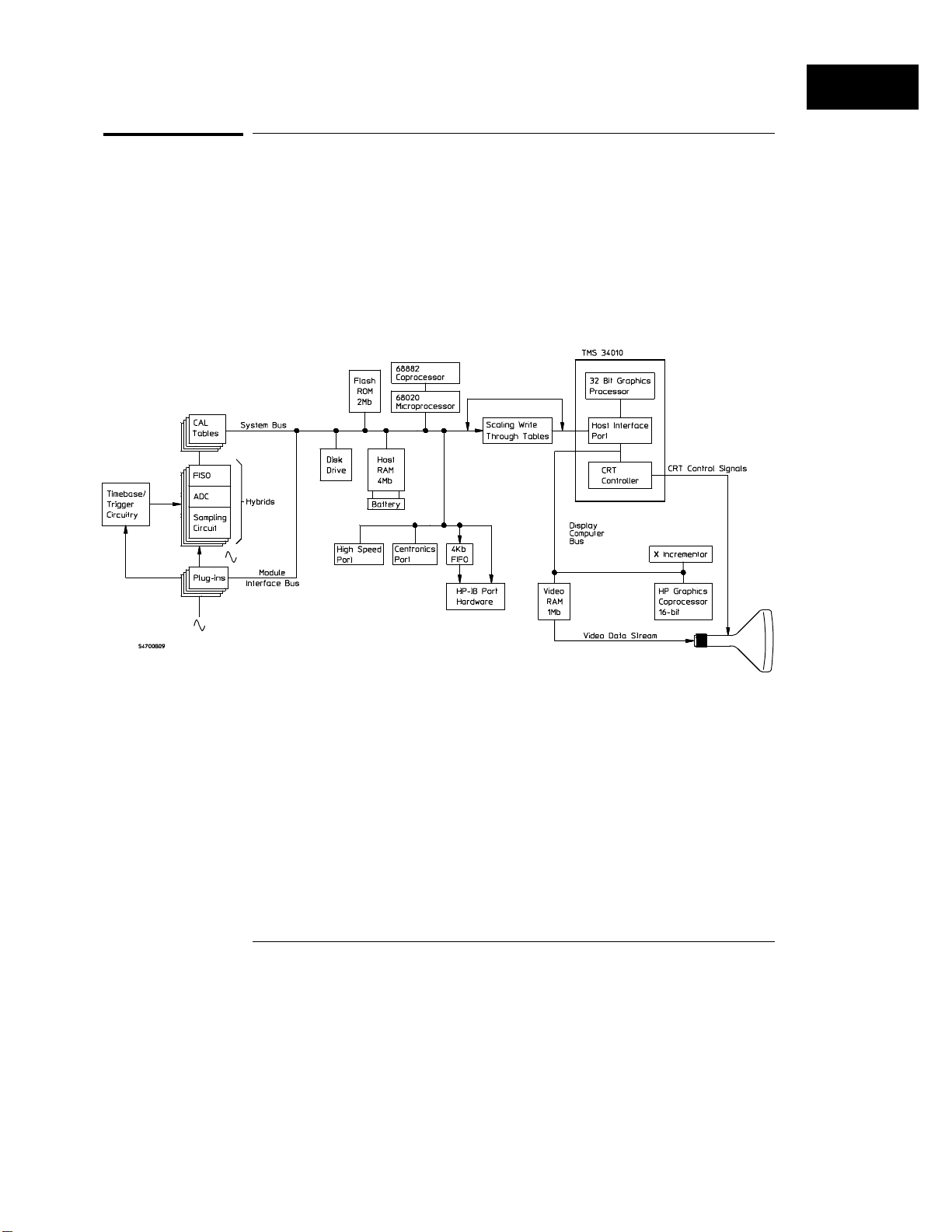
Figure 1-1

How the Oscilloscope Works

Hardware Architecture

This is a high-level look at the internal hardware of the oscilloscope. You will find a complete block diagram of the oscilloscope in the Service Guide that is supplied with the oscilloscope.

Figure 1-1 is a functional block diagram of the hardware in the oscilloscope.

1–3

How the Oscilloscope Works

Hardware Architecture

Hybrid

hybrid contains the following:

•

The signal is sampled by the 500-MSa/s sampler, converted to a digital signal, and then stored into the 4K FISO (fast-in-slow-out) memory.

In the real-time sampling mode the four 500-MSa/s sampling paths are interleaved to achieve a 2-GSa/s sampling rate with 16K of memory behind each plug-in slot on the A model mainframes (64K on the D model mainframes). However, the HP 54721A plug-in, for example, uses two slots which interleaves two hybrids in time to give you a 4-GSa/s sample rate and 32K (128K on the D models) of memory. The HP 54722A plug-in uses four slots which interleaves four hybrids in time to give you 8-GSa/s sample rate and 64K (256K on the D models) of memory.

In the equivalent-time sampling mode, the 500-MSa/s samplers are synchronized and the voltage reference of the ADCs is shifted in voltage by one-quarter of a least significant bit to achieve higher vertical resolution. This process results in 500 MSa/s and 16K (64K on the D models) of memory behind each plug-in slot. In this mode, the HP 54721A plug-in, for example, gives you a 500-MSa/s sample rate and 32K (256K on the D models) of memory.

When viewing a signal that happens either once or infrequently, the preferred acquisition mode is the real-time sampling mode because the higher sampling rate gives a higher single-shot bandwidth. When viewing signals that occur repetitively, the equivalent-time sampling mode is the preferred choice because of the higher system bandwidth and vertical resolution.

Behind each plug-in slot in the mainframe is a hybrid. The

A quad, 500-MSa/s, 2-GHz bandwidth, bipolar, sampling IC Four, 6th order, low-pass, thickfilm, IF filters Two, dual, 500 MSa/s, bipolar, ADC ICs Two, dual, 4K, FISO, memory ICs.

1–4

How the Oscilloscope Works

Hardware Architecture

Plug-in

the input signal, sets the bandwidth of the system, and allows you to choose the input coupling and input impedance. One output of the plug-in is an analog signal that is applied to the hybrid on the acquisition board inside of the mainframe, another output is a trigger signal that is sent to the time base/trigger board.

CAL Table

the sampled data. The result is referred to as adjusted data, and it is sent to the system bus. The CAL table increases the throughput of the oscilloscope because the CPU now reads calibrated data, and does not have to explicitly correct it. This is faster than using a software solution.

Microprocessors and coprocessors

microprocessors, one 32-bit coprocessor, and one 16-bit coprocessor in the mainframe.

•

The plug-in is for analog signal conditioning. The plug-in scales

The CAL table automatically adds the calibration factors to

There are two 32-bit

Motorola 68020 A 32-bit microprocessor that controls the system hardware, and also acts as a traffic controller on the system bus.

Motorola 68882 A 32-bit coprocessor that performs all of the floating point math.

TMS34010 A 32-bit microprocessor that draws data on the display. HP custom graphics coprocessor A 16-bit coprocessor that controls the

gray scale persistence mode, and also writes blocks of data (like the markers and display background) to the display.

1–5

How the Oscilloscope Works

Hardware Architecture

Host RAM

The host RAM is 4 Mbytes of nonvolatile RAM. This is where the waveform data is held and manipulated. In addition, this is the location of the current front-panel setup, setup memories, and waveform memories.

Flash ROM

The flash ROM contains the system firmware that controls the operation of the oscilloscope. You can load new system firmware into the oscilloscope by using the disk drive.

Disk Drive

The disk drive is a 3-1/2 inch, high-density, MS-DOS



compatible disk drive. You can use the disk drive to load system firmware into the flash ROMs, load applications, save screen dumps in a TIFF, GIF, or PCX format, or as additional storage space for saving waveforms and front-panel setups.

User Interface Hardware

The user interface hardware is the keyboard, and the hardware that interfaces the keyboard and knob with the system bus.

FIFO and HP-IB Hardware

The FIFO is a first-in-first-out memory that transfers waveforms through the HP-IB bus under hardware control. This hardware control is much faster than the software control used by other oscilloscopes. The FIFO increases the HP-IB throughput of the oscilloscope.

MS-DOS

1–6

is a US registered trademark of Microsoft Corporation.

How the Oscilloscope Works

Hardware Architecture

See Also

Centronics Port

printers that are compatible with the Centronics interface.

High-Speed Port

this time.

Video RAM

image. The video RAM also contains the pixel memory.

Display

"Display" in Chapter 2 for additional details.

The display is a 9-inch, high-resolution, color display.

The Centronics port is a parallel connector for

The high-speed port feature is not implemented at

This is 1 MByte of fast video RAM for storing the display

1–7

Figure 1-2

How the Oscilloscope Works

Data Flow

The data flow gives you an idea of where the measurements are made on the acquired data, and when the post acquisition signal processing is applied to the data.

Figure 1-2 is a data flow diagram of the oscilloscope. The diagram is laid out serially to give you a visual perception of how the data is affected by the oscilloscope.

1–8

How the Oscilloscope Works

Data Flow

The digitizer samples the applied signal and converts it to a digital signal. The FISO holds the data until the system bus is ready for the data. The output of the FISO is used as an address to the calibration read-through table (cal table). The cal table automatically applies the calibration factors to the data.

In the real-time sampling mode, the calibrated data is stored in the channel memories before any of the postprocessing is performed. Postprocessing includes turning on or off the digital bandwidth limit filter or the interpolator, calculating functions, storing data to the waveform memories, transferring data over the HP-IB bus, or transferring data to and from the disk. Notice that the measurements are performed on the real-time data after it has gone through postprocessing.

Therefore, you can make measurements on the data, and you can turn on or off digital bandwidth limit or interpolation without having to reacquire the data. This is important because the real-time sampling mode is primarily used on events that happen either once or infrequently, and reacquiring the data may not be one of your options. Also, turning on interpolation usually improves the repeatability of your measurements.

The equivalent-time sampling mode is slightly different. Notice that averaging is turned on or off before the data is stored in the channel memories. That means once the data is acquired, if you need to turn averaging on or off before making any measurements, you must reacquire the data. However, because the equivalent-time sampling mode is primarily used on repetitive signals, you should be able to reacquire the data.

1–9

How the Oscilloscope Works

Data Flow

Also, you may notice that postprocessing the data in the equivalent-time signal path includes calculating functions, storing data to the waveform memories, transferring data over the HP-IB bus, or transferring data to and from the disk.

After the measurements are performed, the data is sent through the display portion of the oscilloscope. Notice that connected dots is a display feature, and that it has no influence on the measurement results. The pixel memory is also part of the video RAM, which is past the point where the measurements are performed on the data. Therefore, you cannot make measurements on data in the pixel memory. But, you can make measurements on data stored to the waveform memories.

1–10

How the Oscilloscope Works

Sampling Overview

This gives you a brief overview of sampling. For more details on sampling techniques, refer to Feeling Comfortable with Digitizing Oscilloscopes that is supplied with your oscilloscope. You can also get a copy of HP product note 54720A-1, Bandwidth and Sampling Rate in Digitizing Oscilloscopes, by contacting you nearest Hewlett-Packard Sales Office or by calling the Hewlett-Packard Customer Information Center at 1-800-452-4844.

Real-time sampling

In the real-time sampling mode, all of the data is acquired from one time base sweep. As with any digitizing oscilloscope, the more data that is acquired, the better the oscilloscope can reproduce the waveform on the display. Therefore, this sampling mode has a maximum sampling rate of 2-GSa/s on each plug-in slot. A two-wide plug-in, like the HP 54721A, uses two plug-in slots for a maximum sampling rate of 4 GSa/s. A four wide plug-in, like the HP 54722A, uses four plug-in slots for a maximum sampling rate of 8 GSa/s. Also, this sampling mode is typically used on signals that happen either once or infrequently. Because you may have only one chance to capture the data, you will want to use the maximum sampling rate available.

A simple fact of real-time sampling is that the higher the sampling rate relative to the bandwidth of the signal, the better the oscilloscope can reconstruct the signal. The oscilloscope can best reproduce signals when the sample rate is about four times or greater than the highest frequency components in the signal. That is why the HP 54713A plug-in has a 500-MHz bandwidth. It uses one slot, and one-fourth of 2 GSa/s is 500 MHz. The HP 54721A plug-in has a bandwidth of about 1 GHz because it uses two slots, and one-fourth of 4 GSa/s is 1 GHz.

1–11

Figure 1-3

How the Oscilloscope Works

Sampling Overview

Figure 1-3 shows a 489-ps pulse sampled at 1 GSa/s. You may notice that there are ten different acquisitions. From the picture in figure 1-3, it is difficult to get a sense of what the signal looks like. Any of the ten traces, or none of them, may represent the signal. You can say that the signal in figure 1-3 is undersampled because not enough data was acquired on each time base sweep for the oscilloscope to accurately reconstruct the waveform on the display. Also notice the measurement results at the bottom of the picture. The question marks indicate that there was insufficient data to make the measurements.

1–12

Figure 1-4

How the Oscilloscope Works

Sampling Overview

Figure 1-4 shows the same 489-ps pulse sampled at 2 GSa/s. Notice that ten acquisitions were taken again. This time you have a better sense of what the signal looks like. However, there are still enough differences among each of the ten waveforms that you can say the signal is undersampled. Notice that figure 1-4 gives you more information about the signal than figure 1-3. The oscilloscope has enough data to make the measurements, but the statistics results show that there is a wide variation in the measurement results.

1–13

Figure 1-5

How the Oscilloscope Works

Sampling Overview

Figure 1-5 shows the same 489-ps pulse sampled at 4 GSa/s. You cannot tell from the picture, but there are still ten acquisitions. Notice that the oscilloscope now acquires enough data on each acquisition so that it can more faithfully reconstruct the signal. Also notice that the statistics results indicate that the measurements are much more repeatable.

Use the real-time sampling mode when:

The signal occurs once or infrequently.

•

The sample rate is four times or greater than the highest frequency

•

components (that you are interested in) in the signal.

1–14

How the Oscilloscope Works

Sampling Overview

Equivalent-time sampling

The equivalent-time sampling mode is typically used on repetitive signals, which allows the oscilloscope to acquire data continuously. The sample rate is 500 MSa/s, but the data from many acquisitions are interleaved, which results in a much higher effective sample rate.

You can still use the equivalent-time sampling mode for single-shot applications. Because the interpolation filter is not available in the equivalent-time mode, the maximum single-shot frequency you can reasonably view and also avoid aliasing is about one-tenth the sample rate, or 50 MHz.

The HP 54711A and HP 54712A plug-ins are best suited for equivalent-time sampling because they allow access to the highest system bandwidths.

1–15

Figure 1-6

How the Oscilloscope Works

Sampling Overview

Figure 1-6 shows the same 489-ps pulse as figure 1-4. Because the signal is repetitive, the sampling mode was changed from real time to equivalent time. You may notice how the increased system bandwidth and higher effective sample rate results in excellent reconstruction of the signal. Compare the similarity between figures 1-5 and 1-6. Also notice that the statistical results indicate very repeatable measurement results.

Use the equivalent-time sampling mode when:

The signal is repetitive.

•

The signal contains frequency components, that you are interested in,

•

greater than one-fourth maximum the sample rate of the oscilloscope.

1–16

How the Oscilloscope Works

Choosing Plug-ins

The accuracy of your measurement results depends on the configuration of your oscilloscope system. Part of the configuration is knowing how to set up the various menus that are described in this book for your application. The rest of the configuration is comprised of choosing the plug-ins and probes to use for the measurement. There are several plug-ins available for the oscilloscopes, and you need to pick the plug-in that best matches your application.

When picking a plug-in, you also need to think about the rise time of the oscilloscope compared to the rise time of the signal you are measuring.

The oscilloscope rise time is about:

See Also

Scope Rise Time =

To obtain a rise time measurement accuracy of 5 percent, the rise time of the oscilloscope should be one-third the rise time of the signal you are measuring.

To obtain a rise time measurement accuracy of 1 percent, the rise time of the oscilloscope should be one-seventh the rise time of the signal you are measuring.

The measured rise time is about:

Measured Rise Time =

"Choosing Probes" later in this chapter for information on selecting the correct probe for your application.

0.35

Bandwidth

√



Actual Rise Time2 + Scope Rise Time

1–17

How the Oscilloscope Works

Choosing Plug-ins

Table 1-1 shows the common characteristics for the channel plug-ins.

Table 1-1

Characteristic HP 54711A HP 54712A HP 54713B HP 54714A HP 54721A HP 54722A

Sample Rate 2 GSa/s 2 GSa/s 2 GSa/s 2 GSa/s 4 GSa/s 8 GSa/s Bandwidth in A models 1.5-GHz 1.1-GHz 500-MHz 400-MHz 1.1-GHz 1.5-GHz in D models 2.0-GHz 1.1-GHz 500-MHz 400-MHz 1.1-GHz 2.0-GHz Channels 111211 Memory depth in A models 16K 16K 16K 8K/chan 32K 64K in D models 64K 64K 64K 32K/chan 128K 256K Trigger Ext. (2.5-GHz) Internal Internal Internal Internal/Ext. Ext. (2.5-GHz) Logic trigger No Yes Yes Yes Yes Yes Max. Sensitivity 20 mV/div 10 mV/div 7 mV/div 7 mV/div 10 mV/div 80 mV/div * (with software expansion) Input resistance

Slots used111124

2 mV/div 1 mV/div 1 mV/div 1 mV/div 1 mV/div 8 mV/div

Ω

1 M Ω/50

Ω

1 M Ω/50

Ω

*The standard 1-2-5 sequence in the 54722A plug-in, which is selected by the mainframe’s front-panel knob, does not correspond exactly to the attenuator ratios in the hardware. Refer to the HP 54722A Attenuator Plug-in User’s Reference for more information about the attenuator ranges.

Use the HP 54711A plug-in when:

The signal is repetitive, and you are using the equivalent-time sampling

•

mode. You need high equivalent-time bandwidth.

•

You can use external triggering, and you need high trigger bandwidth.

•

You can give up logic triggering.

•

Use the HP 54712A plug-in when:

The signal is repetitive, and you are using the equivalent-time sampling

•

mode. The signal happens once or infrequently, you are using the real-time

•

sampling mode, and the input signal does not contain any frequency components above 500 MHz.

You need internal triggering.

•

1–18

How the Oscilloscope Works

Choosing Plug-ins

Use the HP 54713B plug-in when:

The signal happens once or infrequently, and you are using the real-time

•

sampling mode. Your application requires only 500-MHz bandwidth, (rise time is slower

•

than 2.1 ns) and you need more than 2 channels. You application requires a 1 MΩ input because you are using a

•

passive-compensated divider probe.

Use the HP 54714A plug-in when:

Your application requires up to 8 channels.

•

Use the HP 54721A plug-in when:

The signal happens once or infrequently, and you are using the real-time

•

sampling mode. You need the 1.1-GHz real-time bandwidth (rise time is slower than 1 ns).

•

You need the 4-GSa/s sample rate.

•

You need 32K memory depth.

•

Use the HP 54722A plug-in when:

The signal happens once or infrequently, and you are using the real-time

•

sampling mode. You require the 8-GSa/s sample rate.

•

You need high, real-time bandwidth.

•

Your application requires high trigger bandwidth, and you can use external

•

triggering.

1–19

Figure 1-7

How the Oscilloscope Works

Choosing Probes

Two problems arise when you use a probe to connect an oscilloscope to a circuit. First, the probe degrades the circuit under test. The new circuit behaves differently than does the circuit without the probe. The behavior you see is the behavior of the circuit with the probe. Second, the transfer function of the probe is part of the overall measurement system response, degrading measurement accuracy.

The probe is a part of the circuit under test

Suppose that you are trying to debug an intermittent failure in a state machine that is implemented in high-speed CMOS logic. You know that you need a high-performance digitizing oscilloscope, but you don’t know which probe gives the best results.

There are two major factors influencing probe selection: the load the probe imposes on the circuit, and the required bandwidth of the circuit with the probe.

1–20

Figure 1-8

How the Oscilloscope Works

Choosing Probes

Probe Loading

Figure 1-8 shows a simplified diagram of the circuit with the probe attached to indicate the principal loading effects. The probe load has both resistive and capacitive components. In addition to this, the inductance in the probe ground lead can cause ringing.

Simplified equivalent circuit of DUT and probe

1–21

Figure 1-9

How the Oscilloscope Works

Choosing Probes

The resistance of the probe to ground forms a divider network with the source resistance of the circuit under test. This reduces the signal amplitude and the dc offset. For example, if the probe’s resistance is 9 times the Thevenin output resistance of the circuit under test, the amplitude is reduced by about 10 percent. See figure 1-9. The frequency-independent amplitude errors and dc offset errors introduced by probe resistive loading are approximately proportional to the ratio of the probe’s resistance to ground and the equivalent output resistance of the circuit under test.

Reduced amplitude and dc offset caused by probe loading

1–22

Figure 1-10

How the Oscilloscope Works

Choosing Probes

The capacitance of the probe tip to ground forms an RC circuit with the output resistance of the circuit under test. The time constant of this RC circuit slows the rise time of any transitions, increases the slew rate, and introduces delay in the actual time of transitions. The approximate rise time

of a simple RC circuit is 2.2 RC. Thus, for an output resistance of 100 Ω and a probe tip capacitance of 8 pF, the real rise time at the node under test cannot be faster than approximately 1.8 ns. Although, it might be faster without the probe.

If the output of the circuit under test is current-limited (as is often the case for CMOS), the slew rate is limited by the relationship dV/dT = I/C. See figure 1-10.

Effects of probe capacitance

1–23

How the Oscilloscope Works

Choosing Probes

Perhaps you have connected an oscilloscope to a circuit for troubleshooting only to have the circuit operate correctly after connecting the probes. The capacitive loading of the probes can attenuate a glitch, remove ringing or overshoot, or slow an edge just enough that a setup or hold time violation no longer occurs.

The inductance of the probe ground lead forms an LC circuit with the probe’s capacitance and the output capacitance of the circuit under test, including any parasitic capacitance of PC board traces, and so on. The ringing frequency of this circuit is:

2 π

√

0.35

Signal Rise Time

F =

If the rise time of the signal is sufficient to stimulate this ringing, then it can appear as part of the captured signal. An approximation of the bandwidth of the signal is:

Signal Bandwidth =

To calculate the ringing frequency, you can assume that the probe ground wire has an inductance of approximately 25 nH per inch. So, a probe with a tip capacitance of 8 pF and a 4-inch ground wire has a ringing frequency of approximately 178 MHz (not considering the circuit capacitance). Here, a signal with a rise time of less than 1.9 ns can stimulate ringing.

1–24

How the Oscilloscope Works

System Bandwidth

The bandwidth of the combined oscilloscope and probe system must be sufficient to accurately reproduce the input signal. Otherwise, time-interval measurements are inaccurate. For example, if the oscilloscope and probe have a combined rise time of 1 ns, and the signal also has a 1-ns rise time, the measured rise time is:

√

The answer is in error by 41 percent. If the oscilloscope and probe have a combined rise time of 330 ps, and the

signal has a 1-ns rise time, the measured rise time is:

√

Now the error is only 5 percent. There are three rules worth memorizing. First, the combined system rise

time (oscilloscope and probe) should be less than 1/3 the rise time of the measured signal for an error of less than 5 percent, or less than 1/7 of the rise time of the measure signal for an error of less than 1 percent. Second, rise time and bandwidth are inversely related as shown in equations 5 and 6. Third, rise times add approximately as the square root of the sum of the squares.

For example, if the oscilloscope and the probe each have 1-GHz bandwidths, the combined bandwidth is approximately 707 MHz and the combined rise time is approximately 495 ps. Therefore this combination could be used confidently to measure actual signal rise times of 1.5 ns with less than 5 percent error, or 3.5 ns with less than 1 percent error.

)

(

)

(

330

(

)

1.41 ns

= 1.05 ns

)

1–25

How the Oscilloscope Works

System Bandwidth

Probe Types

There are three common types of oscilloscope probes. Each type has different loading effects. First, there is the low-impedance resistive divider probe, like the HP 54006A. Second, is the compensated, high-resistance passive divider probe, like the HP 10430A. Third, there is the active probe, like the HP 54701A.

Figure 1-11

Resistive Divider Probes

Resistive divider probes are designed for oscilloscopes with a 50-Ω input impedance. The tip of the probe has a 450-Ω or 950-Ω series resistor. The cable is designed for a 50-

Ω

transmission line. Because the cable is terminated in 50 Ω at the oscilloscope input, it looks like a purely resistive 50-Ω load when viewed from the tip. Therefore the resistive divider is flat over a wide range of frequencies, limited primarily by the parasitic capacitance and inductance of the 450-Ω or 950-Ω resistor and the fixture that holds it. The input resistance of the probe to the circuit under test is either 500 or 1 kΩ.

Resistive divider probe

Ω

1–26

How the Oscilloscope Works

System Bandwidth

Because of the physical geometry of this type of probe and because the divider does not have to be capacitively compensated, this type of probe has the lowest capacitive loading of any probe. This low capacitance and its inherent wide bandwidth make it best suited for wide bandwidth measurements or those measurements where timing is the most critical parameter.

The disadvantage of this type of probe is its relatively heavy resistive loading. Not all circuits can drive 500 Ω or 1 kΩ. Even for measurements in a relatively low impedance circuit, the amplitude errors can be significant. Changes in bias levels or operating current in the circuit under test might affect the circuit’s behavior.

This type of probe is the best choice for minimum disturbance probing of ECL circuits and 50-Ω transmission lines. The 1-kΩ divider probes are also usually suitable for high-speed CMOS circuits. If you are interested in troubleshooting CMOS, consult the data sheet for the particular CMOS part to make sure that it can drive a 1-kΩ load and to determine what the voltage error would be.

Compensated Passive Divider Probes

of oscilloscope probe. The 900-kΩ resistor in the tip forms a 10:1 voltage divider with a 111-kΩ resistor in parallel with the 1-MΩ input resistance of the oscilloscope. Some versions use a 9-MΩ resistor at the tip; the oscilloscope’s input resistance forms the other part of the voltage divider.

This is the most common type

1–27

Figure 1-12

How the Oscilloscope Works

System Bandwidth

To have a flat frequency response, the voltage divider must be compensated for the capacitance of the cable and the oscilloscope or logic analyzer’s input capacitance. One of the compensating capacitors is made adjustable so you can optimize the step response flatness because the input capacitance of the oscilloscope is unknown. The HP 54720A provides a square wave at the calibrator output for this purpose.

Compensated passive divider probe

1–28

Figure 1-13

How the Oscilloscope Works

System Bandwidth

Not all 1-MΩ divider probes work with all 1-MΩ oscilloscope inputs. The probe data sheet shows the range of oscilloscope input capacitance it can accommodate. You must make sure that the input capacitance of the oscilloscope is within that range.

The advantage of this type of probe is that it has the highest resistance. Its disadvantages are that it has the highest capacitive loading and the lowest bandwidth. At 2 MHz, the impedance of an 8-pF capacitance is 10 kΩ, and at

100 MHz it is only 200 Ω. This type of probe is often referred to as a "high impedance" probe. This is a misnomer because they exhibit high impedance only at relatively low frequencies. Figure 1-13 shows a plot of the impedance of a typical 1-MΩ, 8-pF probe as a function of frequency.

Some applications where 1-MΩ (or higher) probes are appropriate include high-impedance nodes (≥ 10-kΩ), and summing junctions in operational amplifiers where the junction voltage is not at dc ground.

Impedance of a 1-MΩ, 8 pF probe versus frequency

1–29

How the Oscilloscope Works

System Bandwidth

Active Probes

An active probe, like the HP 54701A, has a buffer amplifier at the tip. See figure 1-14. This buffer amplifier drives a 50-Ω cable terminated in 50 Ω at the oscilloscope input. Active probes offer the best overall combination of resistive loading, capacitive loading, and bandwidth, even though an active probe does not have the highest resistance, highest bandwidth, or lowest capacitance available. The disadvantages of active probes, besides their higher cost, are the larger size of the tip and a somewhat limited input dynamic range. Previous active probe designs were more susceptible to damage, particularly to ESD, and required careful handling. The HP 54701A is designed to withstand 200 V peak ac and 12 kV of ESD, so it functions reliably in adverse conditions.

The HP 54701A has sufficient bandwidth (2.5 GHz), sufficiently small capacitive loading (0.6 pF), and sufficiently high resistance (100 kΩ) to be useful for both ECL and CMOS circuits, and for most analog circuits.

For the high-speed CMOS state machine in the example, the HP 54701A active probe offers the best combination of measurement accuracy with minimal circuit loading.

Figure 1-14

Active probe

1–30

How the Oscilloscope Works

System Bandwidth

Summary

There is no such thing as the perfect probe, so you must use some discretion in choosing the best type of probe for each measurement.

To make the correct choice, it’s helpful to know the equivalent circuit of the circuit under test. For truly demanding measurements, it may be worthwhile to simulate the effect of the probe using SPICE. This discussion assumes a simple resistance as the equivalent circuit for the circuit under test. For an actual measurement, a more complete model is useful in evaluating the effects of the probe.

Some knowledge of the expected signal, particularly its rise time or spectral content, is also useful in making a probe choice.

Finally, it’s important to know what parameter (voltage or time) you need to measure most accurately, because some tradeoff is almost always required.

1–31

Table 1-2

How the Oscilloscope Works

System Bandwidth

Table 1-2 shows characteristics of recommended probes for the oscilloscope. The bandwidth shown in the table is the overall system bandwidth when used with the listed plug-in and the mainframe.

HP 54701A Active Probe

Input resistance Input capacitance Division Ratio 10:1

Offset range

When used with Bandwidth Maximum sensitivity

HP 54711A 1.3 GHz 20 mV/div HP 54712A 1 GHz 10 mV/div HP 54713B 500 MHz 10 mV/div HP 54721A 1 GHz 10 mV/div

HP 54006A Passive 50-Ω Divider Probe

Input resistance Input capacitance Typically 250 fF

Division Ratio 10:1 or 20:1

When used with Bandwidth Maximum sensitivity

HP 54711A 1.5 GHz 20 mV/div (10:1) or 40 mV (20:1) HP 54712A 1.1 GHz 10 mV/div (10:1) or 20 mV (20:1) HP 54721A 1.1 GHz 10 mV/div 10:1) or 20 mV (20:1)

100 k

Ω

0.6 pF

≤

50 Vdc

500 Ω (10:1) or 1000 Ω (20:1)

HP 10430A 1-MΩ Passive Probe

Input resistance Input capacitance Division Ratio 10:1

When used with Bandwidth Maximum sensitivity

HP 54713B 500 MHz 10 mV/div

1 M

6.5 pF

≤

Ω

1–32

Autoscale Key 2–3 Clear Display Key 2–3 Display 2–4 Entry Devices 2–7 Fine Mode 2–8 Help Menu 2–9 Indicator Lights 2–10 Local Key 2–12 Run Key 2–13 Stop/Single Key 2–14

Front-Panel Features

This chapter describes the display, indicator lights, entry devices, and hardkeys that do not display menus on the screen. Those hardkeys that display menus are described in chapters that follow.

Understanding the information in this chapter will help you in operating the oscilloscope. Information on how to use the front-panel interface is in the User’s Quick Start Guide that is supplied with the oscilloscope.

The two types of keys on the front panel are hardkeys and softkeys. A hardkey has text, numbers, or graphics printed on it; or, it is blue in color. Softkeys are to the right side of the display, and the label for a softkey is displayed on the screen next to that softkey. These labels are referred to as menus, and which menu is displayed depends on the hardkey you press. Not all hardkeys cause softkey menus to display on the screen.

2–2

Front-Panel Features

Autoscale Key

The Autoscale key causes the oscilloscope to quickly analyze the signal. Then, it sets up the vertical, horizontal, and trigger to best display that signal. Autoscale can find repetitive signals with a frequency greater than or equal to 50 Hz, a duty cycle greater than one percent, and an amplitude of 50 mV p-p or greater.

Autoscale looks for signals on all channels, even if they are turned off. Also, autoscale searches for a trigger signal on the external trigger inputs before searching the channel inputs for a trigger signal.

You may find situations where you have pressed the Autoscale key unintentionally. When this happens, you can use the Undo Autoscale key to return the oscilloscope to the settings prior to pressing the Autoscale key.

To undo an Autoscale

Press the blue shift key, then press the Autoscale key again.

Clear Display Key

The Clear display key erases all channel and function waveform data from the graticule area, and it resets all associated measurements and measurement statistics.

When the oscilloscope is stopped

If the oscilloscope is stopped, the display remains cleared of waveform data until the trigger circuit is rearmed and the oscilloscope is triggered. Then, the new data is displayed and measurements are recalculated.

When the oscilloscope is running

If the oscilloscope is running, new waveform data is displayed on the next acquisition and all measurements are recalculated.

2–3

Front-Panel Features

Display

The oscilloscope has a 9-inch, high-resolution, color display. This display is divided up into several areas that are shown in figure 2-1.

Status area

The status area displays prompts, messages, error messages, warnings, acquisition status, sample rate in the real-time mode, and the number of averages when averaging is turned on in the equivalent-time mode.

Figure 2–1

Status area

Graticule area

Time base area

Channel and measurement results area

Memory bar

Time base reference indicator

Time base position setting

Softkey menu area

Marker results and statistics results area

2–4

Front-Panel Features

Display

Graticule area

The graticule area is also referred to as the waveform viewing area. This is where all the waveform data and markers are displayed on the screen.

Time base area

The time base area lists the time base scale setting, reference location, and position setting. You may notice that the reference location is indicated by an arrow. In the figure, the time base settings are:

Scale is 10 ns/div

•

Reference is set to the center of the graticule area

•

Position is −9.8 ns

•

Channel and measurement results area

The channel settings and measurement results share the same area. The channel settings are displayed only when the measurements are off. When you make an automatic measurement, the results are displayed in place of the channel settings.

To get the channel settings back on the display

Press the blue shift key, then press the Clr meas (clear measure) key.

When a channel number is displayed, it indicates that the channel is turned on. In the figure 2-1, the channel settings are:

Channel 1 is on, scale is 85 mV/div, offset is −166 mV.

•

Channel 2 is on, scale is 50 mV/div, and offset is 100 mV.

•

Channels 3 and 4 are turned off.

•

2–5

Front-Panel Features

Display

Marker results and statistics results area

The marker results and statistics results share the same area. The statistics results are displayed only when the manual and waveform markers are turned off, or when the measurement marker readout is turned off.

Softkey menu area

The softkey menus are displayed in this area. Which menu is displayed depends on the hardkey you press. The Quick Start Guide contains an explanation of how the softkeys operate.

Memory bar

The memory bar represents the entire waveform record. The highlighted part of the memory bar represents the portion of the waveform record that is currently on the display. When possible, the acquisition hardware is set up so that all of the waveform record is displayed on the screen. When the waveform record contains more data than the display has resolution (number of pixels), there can be more than one data point per pixel column on the display.

2–6

Front-Panel Features

Entry Devices

The entry devices are the knob, arrow keys, and keypad. You can use the entry devices to change the numeric setting of some softkeys, like trigger level, or to select an item from a list of choices.

When you use the entry devices to scroll through a list of choices, you may notice that the background color of each item changes as scroll through the list. Occasionally, a particular feature may not be available with a specific plug-in model. In this case, the background color of that feature will not change as you scroll through the list.

2–7

Front-Panel Features

Fine Mode

The fine mode allows you to change the channel scale, offset, and time base scale in smaller increments using the knob than the knob normally allows. For example, on most plug-ins the knob changes the channel scale in a 1-2-5 sequence, like 100 mV, 200 mV, and 500 mV. In the fine mode, the knob changes the channel scale in smaller increments, like 100 mV, 101 mV, 102 mV.

To put the oscilloscope in the fine mode, press the blue key on the keypad, then press the down arrow key with the word "Fine" written above it. Repeat the process to exit the fine mode.

You can tell when the fine mode is active because the screen displays the word "FINE" at the top-right corner of the graticule area.

2–8

Front-Panel Features

Help Menu

The help menu is designed to aid you in finding the initial key sequence to execute a particular feature. When you press the Help key, a three-column index is displayed on the screen. The left column lists the features of the oscilloscope, the middle column lists the hardkey key, and (if needed) the right column lists the softkey you press to find that feature. You can use either the knob or arrow keys to scroll through the list of features.

For example, to move a signal vertically on the display, you can look up Channel vertical position in the help menu list. The middle column indicates that you press the Channel hardkey, and the right column indicates that you also press the Offset softkey. Offset allows you to move waveforms vertically on the display.

When possible, the feature is listed under different names. This allows you to look up a feature by a name that is more familiar to you. For example, you could have also looked for position (vertical), vertical offset, or vertical position. Each of these titles give you the same key sequence to follow.

Figure 2-2

2–9

Front-Panel Features

Indicator Lights

There are three indicator lights near the top-left corner of the oscilloscope. These lights can give you a quick indication about the acquisition status of the oscilloscope.

Armed

When the armed light is turned on, it indicates that the trigger circuit is armed and waiting for a valid trigger event to occur. A valid trigger event occurs when a signal meets the triggering conditions set up in the trigger menu.

In single-shot applications, when the armed light turns off, you know that the oscilloscope has triggered. If the screen does not display any data, the lack of data indicates that you need to change the channel and time base menus to properly display the signal. Also, you may have to reacquire the data after changing the setup conditions on the ocilloscope to display the signal.

Triggered

When the triggered light is on, it indicates that the oscilloscope accepted a trigger event. Every time the oscilloscope accepts a trigger event, it makes one time base sweep and displays the data that is acquired during that sweep.

When you are in the trigger menu and the oscilloscope is internally triggered, a line is displayed that represents the trigger level. You can use this line to help you determine where to set the trigger level on the signal for your application.

2–10

Front-Panel Features

Indicator Lights

When the oscilloscope is externally triggered, there is no such indicator. However, you can use the triggered light to help you determine the trigger thresholds. To do this, simply move the trigger level in either direction. When the triggered light turns off, you know that is one of the trigger thresholds. Move the trigger level in the other direction to determine the other threshold. You now know what the trigger thresholds are and you can set the trigger level accordingly for your application. Typically you set the trigger level half way between the two thresholds.

Auto Triggered

When the auto triggered light is on, it indicates that the oscilloscope is not seeing any valid trigger events, and that the oscilloscope is forcing itself to trigger every 30 ms.

If you see that the auto triggered light is on, you know that the oscilloscope is triggering and that the screen should display data. If the screen is not displaying data, check the channel offset to see if it is set correctly, and check to make sure that the channel display is turned on. If you are using both single-wide and two-wide plug-ins and the memory depth is set to greater than 16K, check the time base position setting.

2–11

Front-Panel Features

Local Key

You get to the local key by pressing the blue shift key on the keypad, followed by pressing the Stop/Single key. The local key tells the oscilloscope to return control to the front-panel. This is the only active key when the oscilloscope is under remote control. The exception occurs when the controller sends a local lockout command. The local lockout command prevents the local key from causing control of the oscilloscope to return to the front panel.

2–12

Front-Panel Features

Run Key

The Run key causes the oscilloscope to resume acquiring data. If the oscilloscope is stopped, it starts acquiring data on the next trigger event. If the oscilloscope is already in the run mode, it continues to acquire data on successive trigger events.

If pressing the Run key does not cause waveform data to display on the screen, try the following hints:

Press the Autoscale key (unless the signal is single-shot).

•

Make sure that a signal is connected to one of the channels and that the

•

display for that channel is turned on. Make sure that the offset does not have the trace clipped off the display.

•

Check the trigger setup conditions to make sure that the trigger conditions

•

are valid for the signal. Set the trigger sweep mode to Auto. Auto sweep forces the oscilloscope to

•

trigger, which may allow you to see enough of the signal so that you can set up the front panel properly.

2–13

Front-Panel Features

Stop/Single Key

Pressing the Stop/Single key causes the oscilloscope to stop acquiring data. The status area of the screen displays the message "Acquisition Stopped." Each subsequent press of the Stop/Single key rearms the trigger circuit. The next trigger event causes the oscilloscope to make a single acquisition, any measurements are recalculated, and the status area of the screen displays the message, "Acquisition Complete." If all of the channels are turned off or if a trigger event is not found, the oscilloscope will not acquire any data.

Capturing single-shot events

Single-shot events are waveforms that occur only once or infrequently. Some examples of single-shot events are a switch closure, a power supply turnon, the impact of an object on the floor, or an errant pulse that causes your system to fail.

In order to capture a single-shot event, you need to have some knowledge of the waveform you are trying to capture. You must know the approximate amplitude, duration, and dc offset so that you can set up the trigger level, vertical scale and offset, and time base controls so that the oscilloscope can capture and display the event.

If you are using a logic family, the two common trigger levels you can use to capture an intermittent glitch are VIH minimum and VIL maximum.

2–14

Front-Panel Features

Stop/Single Key

To capture a single-shot event

1 Connect the signal to the oscilloscope.

2 Press the Channel key (located on the plug-in). Set the channel Display to

on. Then, select the Scale and Offset settings to display the signal vertically.

3 Press the Time base key. Then, select the Scale and Position settings to display the signal horizontally.

4 Press theTriggered key. Then, Set up the trigger menu to best capture the signal. Set the Sweep to triggered.

5 Press Acquisition. Then, set the Sampling mode to real time.

6 Press the Stop/Single key.

This stops the oscilloscope from acquiring any additional data.

7 Press the Clear display key.

This erases any previously acquired data from the display and resets any measurement results.

8 Press the Stop/Single key again.

This rearms the trigger circuit. The next event that meets the trigger criteria specified in step 4 is captured by the oscilloscope. If the channel and time base controls are set correctly, the signal is displayed on the screen and any measurement results are recalculated.

To capture additional data, press the Stop/Single key again. Depending on your application, you can press the Clear display key between acquisitions, or you can allow the display to build a waveform.

To allow the waveform to build on the display, set the display persistence to a long time (several seconds or more) and do not press the Clear display key between acquisitions.

2–15

2–16

Sampling Mode 3–4 Digital BW Limit 3–6 Interpolate 3–6 Sampling Rate 3–12 Record Length 3–14 Averaging 3–19 Completion 3–20

Acquisition Menu

Figure 3–1

Acquisition Menu

The acquisition menu allows you to customize the way the oscilloscope acquires the data. Some of your choices are selecting the sampling mode, number of averages, sample rate, and record length.

Acquisition menu map

3–2

Acquisition Menu

When you press the Acquisition hardkey, the sampling mode you select determines which of these two softkey menus is displayed. The menu on the left is for the real time-time sampling mode, while the menu on the right is for the equivalent-time sampling mode.

3–3

Acquisition Menu

Sampling Mode

The two sampling modes are real time and equivalent time. Real time is primarily used on events that occur either once or infrequently. Equivalent time is primarily used on repetitive signals.

Real time

In the real-time sampling mode, all the data points that make up a waveform come from one trigger event. Therefore, you want the highest sample rate possible to better reconstruct the signal. The real-time sampling mode has the following features:

8 bits of vertical resolution

•

Fast waveform throughput

•

Ability to turn on or off the bandwidth limit filter

•

Ability to turn on or off the interpolator

•

Selectable sample rate

•

Selectable record length

•

3–4

Acquisition Menu

Sampling Mode

The maximum sample rate allows you to have the maximum single-shot bandwidth.

The real-time sampling mode is intended to capture events that happen either once or infrequently. To accurately display infrequently occurring events, you need to capture and display as much data as possible with a single trigger. For example, use the real-time sampling mode for laser applications, high-speed glitch capture in digital systems, eye diagrams, or when looking for transient events.

Equivalent time

In the equivalent-time sampling mode, the waveform is reconstructed from data points that are acquired from multiple trigger events. The equivalent-time sampling mode has the following features:

8 bits of vertical resolution

•

Averaging of acquired data points to achieve vertical resolutions of up to

•

12 bits. Maximum sampling rate of 500 MSa/s on each plug-in slot

•

Maximum system bandwidth

•

Ability to turn on or off averaging

•

Selectable record length

•

Maximum of 32K points for any equivalent-time waveform.

•

The equivalent-time sampling mode is intended for use on repetitive signals. For repetitive signals, you can use the data acquired from multiple triggers to reconstruct the waveform, which gives you a higher system bandwidth.

3–5

Acquisition Menu

Digital BW Limit

Digital bandwidth limit is a low-pass filter that removes high-frequency noise from the waveform. Digital bandwidth limit reduces the bandwidth of the oscilloscope to the current sample rate divided by 20. Digital bandwidth limit improves the vertical resolution of the oscilloscope by reducing both the noise floor in the oscilloscope and any noise riding on the input signal.

It is available in the real time sampling mode only.

•

It is an FIR filter that approximates a Gaussian response.

•

It affects channel waveform data only (not available on functions or

•

memories).

Interpolate

Interpolate is a finite impulse response (FIR) digital filter that makes the best possible reconstruction of the waveform. This reconstruction is done by using digital signal processing (DSP) to add data points between the acquired data points. The interpolated data points are used in calculating measurement results, which usually improves the accuracy of your measurements.

The bandwidth of the FIR filter is

Figure 3-2 shows a single-shot acquisition of a rising edge. Interpolate is turned off, so all you see on the display is a series of dots. However, figure 3-3 shows the same rising edge, except that interpolate is turned on. Interpolate gives you a better sense of what the actual waveform looks like.

3–6

Figure 3–2

Acquisition Menu

Interpolate

Figure 3–3

Interpolation turned off

Interpolation turned on

3–7

Figure 3–4

Acquisition Menu

Interpolate

Interpolate is different from a display feature called connected dots. Connected dots does a linear interpolation by connecting the data points with a straight line. Because this is a display phenomenon, connected dots has no effect on any measurement results. The measurement results are calculated with the data that is in memory rather than what is on the display. Figure 3-4 shows the same rising edge, except that interpolate is turned off, and connected dots is turned on.

For the best measurement results, leave interpolation turned on all the time. Only turn interpolation off when you want to see the actual acquired data points, or when you want to increase the throughput of the oscilloscope.

Connected dots is turned on and interpolation is turned off

3–8

Acquisition Menu

Interpolate

If the applied signal is clipped, digital oscilloscopes cannot accurately reconstruct the signal. Other oscilloscopes do not always give you an indication that the applied signal is clipped, especially if any filters are also turned on. This oscilloscope has a feature that gives you an indication that the data is clipped by not filtering the clipped portion of the waveform. If Interpolate is turned on, connected dots is used instead of interpolation of the clipped data. The following two pages show some examples of clipped waveforms.

Figure 3-5 shows a signal that is not clipped. Figure 3-6 shows the same signal when it is clipped. Notice that connect the dots is used instead of interpolation.

When filters are turned on, like bandwidth limit, it is even more difficult to determine if the applied signal is clipped. Figure 3-7 shows the same signal as figure 3-5, (a signal that is not clipped) and the bandwidth limit filter is turned on.. Figure 3-8 shows the same signal, except that it is now clipped and the bandwidth limit filter is turned on.

3–9

Figure 3–5

Acquisition Menu

Interpolate

Applied signal is not clipped

Figure 3–6

Applied signal is clipped

3–10

Figure 3–7

Acquisition Menu

Interpolate

Figure 3–8

Applied signal is not clipped and bandwidth limit is turned on

Applied signal is clipped and bandwidth limit is turned on

3–11

Acquisition Menu

Sampling Rate

Sampling rate and waveform record length (also called waveform memory) are very closely tied together. Sampling rate determines how often the oscilloscope samples the signal you are measuring, and waveform record length is the amount of memory the oscilloscope must fill up before it updates the measurement results.

Usually, you use a high sample rate, so there are plenty of data points to better reconstruct the original waveform. For fastest throughput, you use a short waveform record because the oscilloscope must fill up the waveform record before it updates the measurement results. The higher the sample rate, the faster any waveform record fills up. A long waveform record slows down the throughput of the oscilloscope. As a result, you must often make a trade-off between sample rate and record length, that also results in measurement speed and accurate reconstruction of the waveform.

If you set the sample rate and record length to automatic, the oscilloscope picks an optimum sample rate and record length that gives the best waveform reconstruction and measurement speed for the time base scale setting you selected. However, you may want to make the trade-off decisions yourself by selecting a sample rate and record length that fits your application. You may prefer to sacrifice measurement throughput by selecting a high sample rate and a long record length, or you may want to have a high sample rate and a short record length to maximize the measurement throughput.

There are some points you should remember when you are mixing plug-ins, (using both single-wide plug-ins and a two-wide plug-in). The maximum sampling rate is 2 GSa/s per plug-in slot. A two-wide plug-in, like the HP 54721A, uses two plug-in slots which allows a maximum sampling rate of 4 GSa/s. A four-wide plug-in, like the HP 54722A, uses four plug-in slots which allows a maximum sampling rate of 8 GSa/s. The selected sample rate is displayed in the acquisition menu and in the status area of the screen. (The upper left corner of the screen is the status area.)

3–12

Acquisition Menu

Sampling Rate

When a single-wide plug-in and a two-wide plug-in are both turned on, both plug-ins sample at the same sample rate up to 2 GSa/s. Above 2 GSa/s, the single-wide plug-in samples at its maximum sample rate of 2 GSa/s while the two-wide plug-in samples at the selected sample rate above 2 GSa/s. Remember, even though you can select a 4-GSa/s sample rate or an 8-GSa/s sample rate, a single-wide plug-in has a maximum sample rate of 2 GSa/s.

If the two-wide is turned off and the single-wide is turned on, the status line displays the actual sample rate up to 2 GSa/s. However, the acquisition menu allows you to select a sample rate up to 4 GSa/s or up to 8 GSa/s. That is because even though the two-wide plug-in or the four-wide plug-in is turned off, if it is used as an operand in a waveform math function, it is acquiring data at the selected sample rate.

Automatic

Automatic lets the oscilloscope select the sampling rate for you. The advantage is that the oscilloscope selects a sample rate that optimizes the way the waveform is displayed and the display update rate.

When the record length is set to manual and sample rate is set to automatic, the oscilloscope selects the highest sample rate that allows all the data in the waveform record to fill the screen.

Manual

Manual lets you pick a sample rate. However, you have to make the trade-off decisions on the interaction among sample rate, record length, and measurement throughput.

3–13

Acquisition Menu

Record Length

Record length sets the memory depth for the waveform record. Record length is available in both the real-time and equivalent-time sampling modes. The choices for record length are automatic or manual.

The time between the sample points equals 1 divided by the sample rate, and the amount of data in memory equals the time between the points times the number of points. For example, if the sample rate is 2 GSa/s and the record length is 400 points, the time between the sample points is 0.5 ns; and, 0.5 ns times 400 points is 200 ns of waveform data stored in the waveform record. Because there are ten horizontal divisions, set the time base to 20 ns/div to display the whole waveform record.

Sample

There are some points you should remember when you are mixing plug-ins, (using both single-wide plug-ins and a two-wide plug-in). The maximum record length is 16K per plug-in slot on the A model mainframes, and up to 64K per plug-in slot on the D model mainframes. A two-wide plug-in, like the HP 54721A, uses two plug-in slots which allows a maximum record length of 32K on the A model mainframes, and up to 128K on the D model mainframes.

When a single-wide plug-in and a two-wide plug-in are both turned on, both plug-ins use the same record length up to 16K (or 64K). Above 16K (or 64K), the single-wide plug-in has still has a maximum record length of 16K (or 64K) while the two-wide plug-in uses the selected record length up to 32K (or 128K). Remember, even though you can select a 32K (or 128K) record length, a single-wide plug-in still has a maximum record length of 16K (or 64K).

Record Length) = Time

(

Rate

Duration of the Record

3–14

Acquisition Menu

Record Length

Automatic

Automatic lets the oscilloscope select the record length for you. The oscilloscope picks a record length that optimizes the amount of data acquired and the display update rate. When the sample rate is set to manual and the record length is set to automatic, the oscilloscope selects the shortest record length that allows all the data in the waveform record to fill the screen (to a lower limit of 256 points for a single-wide plug-in and 512 points for a two-wide plug-in, and to an upper limit of the maximum record length).

When the oscilloscope is in the color graded display, waveform histogram, or mask testing modes, an optimum number of points for the database is selected. It is recommended that the auto record length be used for the above three modes.

Manual

Manual lets you pick a record length from 16 to 16K points with single-wide plug-ins in the A model mainframes, from 16 to 65K points in the D model mainframes. (up to 32K or 128K points with a two-wide plug-in, like the HP 54721A; or up to 64K or 256K points with a four-wide plug-in, like the HP 54722A). Use the knob, arrow keys, or keypad to select a record length. Remember that sample rate and record length work together. If you combine a small record length with a high sample rate, you will have a very fast throughput, but very little data in the record.

3–15

Figure 3–9

Acquisition Menu

Record Length

Figure 3-9 shows a 256-point record length, a 50-ns/div time base scale, and a 2-GSa/s sample rate. Notice that the entire waveform record is displayed. The 2-GSa/s sample rate fills up the 256-point waveform record quickly, which increases measurement throughput, but does not leave much data for the oscilloscope to display.

GSa

(256 Points

⁄

128 ns of data

)

Because the time base is set to 50 ns/div and the screen is 10 divisions wide, the screen can display up to 500 ns of data. In this example, there is 128 ns of data in the waveform record, which is not enough data to fill the screen. In order to fill the screen, either increase the waveform record length to 1000 to capture more data or change the time base scale to 12.8 ns/div.

Manual sample rate and manual record length

3–16

Figure 3–10

Acquisition Menu

Record Length

Figure 3-10 shows the same 256-point record and a 50-ns/div time base scale. However, the sampling rate was set to automatic, so the oscilloscope picks a sample rate of 500 MSa/s to avoid filling up the waveform record too fast and displaying a waveform like figure 3-9. Because the waveform record is only 256 points, the oscilloscope selected a lower sample rate in order to optimize the amount of data stored in memory to fill up the screen. Notice that more data is displayed.

(256 Points) = 512 ns of data

MSa

500

⁄

Because the screen can display up to 500 ns of data, about 97.7 percent of the waveform record is displayed on the screen. The arrow on the right side of the memory bar indicates that the data in the waveform record that is not presently displayed is to the right side of the screen.

Automatic sample rate and manual record length

3–17

Figure 3–11

Acquisition Menu

Record Length

Figure 3-11 shows how the oscilloscope handles the signal if the sample rate and record length are both in the automatic mode. Because of the time base scale setting, the oscilloscope picks a sample rate and record length that optimizes the throughput of the oscilloscope while still displaying most of the waveform record on the screen. Notice that the oscilloscope picked a sample rate of 2 GSa/s and increased the waveform record to 1001 points.

(1001 Points) = 500.5 ns of data

GSa

⁄

The same amount of data is stored in the waveform record as figure 3-10, except that in figure 3-11 the data was acquired at 2 GSa/s instead of 500 MSa/s.

Automatic sample rate and automatic record length

3–18

Acquisition Menu

Averaging

Averaging is available in the equivalent-time sampling mode only. Before updating the display or measurements, the oscilloscope averages the newly acquired data with the existing data. The higher the number of averages, the less impact each new waveform will have on the composite averaged waveform. You can adjust the number of averages from 1 to 4096 with the knob, arrow keys, or keypad.

Averaging significantly reduces noise on the displayed waveform, improves resolution of the displayed waveform, and increases measurement repeatability, all due to a more stable, displayed waveform. However, averaging slows down the throughput of the oscilloscope. Also, the waveform is less responsive to changes, especially when you select a high number of averages.

The vertical resolution can be improved to greater than 12 bits by using averaging.

The oscilloscope uses this formula to calculate how to include new data with existing data.

(new value)]

[

(

)

[

n−1

(

existing value)] .

)

(

3–19

Acquisition Menu

Completion

The Completion control is provided to allow you to make a tradeoff between how often equivalent time waveforms are measured and how much new data is included in the waveform record when a measurement is made. The completion control has no effect in the real-time mode, since the entire waveform record is filled on every trigger. The control is, however, useful in equivalent-time mode because it is possible that as few as 0 new data points are placed in the waveform record as the result of any given trigger event. It can take many trigger events to fill the entire waveform record.

When the Completion control is on, it specifies how many of the data point storage bins (time buckets) in the waveform record must contain a waveform sample before a measurement is made. For example, if Completion is set to 60%, then 60% of the storage bins in the waveform record need to contain a new waveform data sample. If averaging is on, then the criteria is more stringent. At least 60% of the storage bins must contain waveform data values that were averaged the number of times specified by the number of averages control. After the measurement is made, the data in the waveform record is erased and the acquisition process starts over. Due to the nature of the real-time acquisition mode, 100% of the waveform record bins are filled after each trigger event and all of the old data in the record is replaced by new data. Hence, the Completion control really has no effect and the behavior is exactly what is expected if Completion were set to 100%.

When the Completion control is off, the oscilloscope makes measurements on waveforms after each acquisition cycle, regardless of how complete they are. The waveform record is not cleared after each measurement, rather old data points are replaced by new samples as they become available.

Typically, a 90% completion setting provides very good measurement results. Reaching 100% completion can require substantially more time than reaching 90% when at faster sweep speeds. Depending on the shape of your waveform, you may be able to make accurate measurements with Completion settings of even less than 90%. For a uniform data distribution when using the color graded display, waveform histogram, or mask testing modes, set Completion to 100%.

Selecting default setup or pressing autoscale sets Completion to off.

3–20

Applications

Loading Applications

Because the application is stored in the oscilloscope’s volatile memory, you must reload the application each time the oscilloscope’s power is cycled.

If the scope is turned on.

Place the disk into the disk drive.

Press the Application key at the bottom of the display.

Press the Install Application softkey.

If the scope is turned off.

Place the disk into the disk drive.

Turn on the scope.

The application will load automatically as the scope powers up and will remain loaded in RAM as long as the scope is left turned on. To access the application, press the application key at the bottom of the display.

4–2

Mainframe Calibration 5–3 Plug-in Calibration 5–4 Normal Accuracy Calibration Level 5–5 Best Accuracy Calibration Level 5–6 Probe Calibration 5–8

Calibration Overview

This section briefly explains the calibration of the HP 54720 and HP 54710 oscilloscopes. It is intended to give you or the calibration lab personnel an understanding of the various calibration levels available, and how they were intended to be used. Also, this section acquaints you with the terms used in this manual, the help screens, and the data sheet as they apply to calibrating the oscilloscope.

5–2

Calibration Overview

Mainframe Calibration

Mainframe calibration allows the oscilloscope to establish the calibration factors for each slot independent of the plug-ins. These factors are stored in the oscilloscope’s nonvolatile RAM. Mainframe calibration is initiated from the "Utility/Calibrate/Calibrate Mainframe" menu, or from the key on the front panel of the HP 54717A Calibration Plug-in.

Mainframe calibration should be done on a periodic basis (at least annually), or if the temperature since the last mainframe calibration has changed more than ±5 °C. The temperature change since the last calibration is shown on the calibration status screen which is found under the "Utility/Calibrate/Calibrate Status On" menu. It is the line labeled "Current Frame Temperature ∆: _ °C"

The equipment needed to perform mainframe calibration is:

HP 54717A Calibration Plug-in

•

Three BNC cables (1 to 2 ft, two cables must be the same length)

•

20-dB BNC attenuator

•

BNC Tee

•

When the calibration is initiated, instructions appear on the screen on how to connect the various pieces of equipment to perform the calibration. Note:

you can use the 20-dB attenuator as a 50-Ω terminator. There is a switch on the back panel of the oscilloscope that allows the

mainframe calibration to be enabled or disabled. The rear panel has a drawing that shows the function of each switch and which is the protected position. To prevent access to the mainframe calibration switch, place a sticker over the access hole to this switch.

See Also

The Service Guide for more details about the mainframe calibration, and the position of the rear-panel memory protect switches.

5–3

Calibration Overview

Plug-in Calibration

Plug-in calibration allows the oscilloscope to establish the calibration factors for a particular plug-in independent of the mainframe in which it is calibrated. These calibration factors are stored in the plug-in’s EEPROM, so the factors stay with plug-in, not with the mainframe the plug-in was calibrated in. Plug-in calibration is initiated from the "Utility/Calibrate/ Calibrate Plug-in" menu.

Plug-in calibrations should be done annually or if the plug-in has been repaired or reprogrammed. The equipment needed to perform a plug-in calibration is a BNC cable (1 to 2 ft).

Because the intent is for the oscilloscope to determine the calibration factors for the plug-in only, you should perform plug-in calibrations right after calibrating the mainframe. That way, any drifts in the mainframe calibration (due to time or temperature) will not cause drift in the calibration factors assigned to the plug-in.

Inside the plug-in, there is a switch that enables or disables the ability to write into the plug-in’s EEPROM memory. You must remove the cover of the plug-in to gain access to the switch. To prevent access to the switch, place a sticker on the plug-in cover.

5–4

Calibration Overview

Normal Accuracy Calibration Level

Normal accuracy calibration level refers to the level of accuracy that is achieved when a plug-in is installed in a slot of a mainframe, but has not been calibrated to best accuracy in that particular slot.

The oscilloscope uses the mainframe calibration factors and the plug-in calibration factors to determine the normal calibration factors for that plug-in in that slot.

The intent of this level of calibration is to allow any plug-in to be inserted in any mainframe slot and still achieve a typical vertical accuracy of ±3%.

For two-wide plug-ins, like the HP 54721A, the interleaving of the two mainframe slots is performed during the best accuracy calibration. Therefore, the real-time sampling mode is typically not useful in the normal accuracy mode. For accurate results, a best accuracy calibration must be performed to use two-wide plug-ins in the real-time mode.

See Also

"Best Accuracy" in this chapter for details on the best accuracy calibration. "Normal Accuracy" in chapter 16 for more details on the normal accuracy specifications.

5–5

Calibration Overview

Best Accuracy Calibration Level

Best accuracy calibration level refers to the level of accuracy that is achieved when a plug-in is installed in a mainframe slot and is calibrated to the best accuracy level. A best accuracy calibration is initiated from the "Channel/Calibrate/Calibrate to best accuracy" menu.

The intention is that a recent best accuracy calibration should be performed before critical measurements are made to ensure the best measurement results. The best accuracy calibration is fairly quick and easy, and only a BNC cable is needed to perform the calibration.

The oscilloscope establishes best accuracy calibration factors by calibrating the plug-in and the mainframe slot as a system. These calibration factors are stored in the mainframe’s nonvolatile RAM. The oscilloscope keeps these calibration factors for a plug-in/slot combination until a plug-in with a different serial number is calibrated to best accuracy in that slot. This means that a plug-in that was calibrated to best accuracy in a particular mainframe slot can be removed and reinstalled later in that slot and the best accuracy calibration is still in effect, as long as no other plug-in was placed in that slot and calibrated to the best accuracy level in the meantime.

The best accuracy calibration factors for a two-wide plug-in are stored in the left slot. For example, if you performed a best accuracy calibration on a two-wide plug-in in slots 2 and 3, the best accuracy calibration factors are stored in the memory behind slot two. You can remove the two-wide plug-in and install a single-wide plug-in in slot 3. You can perform a best accuracy calibration on the single-wide plug-in in slot 3 without affecting the best accuracy calibration factors for the two-wide plug-in that are stored behind slot 2.

5–6

Calibration Overview

Best Accuracy Calibration Level

For the best measurement results, a channel (plug-in/slot combination) should be calibrated to best accuracy level. Also, two wide plug-ins must be calibrated to best accuracy level to give accurate results in real-time mode.

The best accuracy calibration level has a temperature ∆ associated with it, just like the mainframe calibration. This temperature ∆ appears in the "Plug-in" calibration status screen for all plug-ins under the "Utility/Calibrate/Cal status on" menu and for each plug-in under the "Channel/Calibrate/Cal status on" menu.

In order for a channel to meet the specifications listed under "Best Accuracy" in chapter 16, both the "Current frame Temp ∆" and the "Best Accuracy Temp ∆" must be between ±5 °C. In other words, the oscilloscope must be within ±5 °C from the temperature that the mainframe was calibrated at and within ±5 °C from the temperature that the best accuracy calibration was calibrated at for a particular plug-in slot calibration.

5–7

Calibration Overview

Probe Calibration

Probe calibration allows the oscilloscope to establish the gain and offset of a probe that is connected to a channel of the oscilloscope, and apply those factors to the calibration of that channel. Probe calibration is initiated from the "Channel/Probe/Calibrate probe" menu.

To achieve the specified accuracy (±2%) with a probe connected to a channel, that channel should be calibrated to the best accuracy level. This ensures the best measurement results.

If the best accuracy is not needed, a probe can be calibrated with a channel that is at the normal-accuracy level. This achieves a typical vertical accuracy of ±4%.

For active probes that the oscilloscope can identify through the probe power connector, like the HP 54701A, the oscilloscope automatically adjusts the vertical scale factors for that channel even if a probe calibration is not performed. For passive probes or nonidentified probes, the oscilloscope adjusts the vertical scale factors only if a probe calibration is performed. If you do not perform a probe calibration but want to use a passive probe, the attenuation factor can be entered in the "Channel/Probe/Probe atten" menu.

You can use the probe calibration to calibrate any network, including probes or cable assemblies. The oscilloscope calibrates the voltage at the tip of the probe or the cable input.

If the probe being calibrated has an attenuation factor that allows the oscilloscope to adjust the gain (in hardware) to produce even steps in the vertical scale factors, the oscilloscope will do so. If the probe being calibrated has an unusual attenuation, like 3.75, the oscilloscope may have to adjust the vertical scale factors to an unusual number, like 3.75 V/div. Typically, probes have standard attenuation factors such as divide by 10, divide by 20, or divide by 100.

5–8

Display 6–4 Scale 6–5 Offset 6–6 Input 6–6 Probe 6–7 Calibrate 6–10

Channel Menu

A plug-in performs analog signal conditioning for the oscilloscope. An HP 54700-series plug-in scales the input signal, sets the bandwidth of the system, and allows you to choose the input coupling that determines the input impedance. The output of the plug-in is an analog signal that is applied to the ADCs that are on an acquisition board inside the mainframe. The plug-in also provides a trigger sync signal to the time base/trigger board inside the mainframe.

This chapter treats the channel menus generically. Specific details about each menu, operating ranges, and specifications depend on which plug-in you are using.

Figure 6-1 is the channel menu map for the HP 54712A Amplifier plug-in. The other plug-ins may have specific features that are not shown on this menu map. The purpose of this menu map is to show you the softkeys that are talked about in this chapter. For specific details about another plug-in, see the User’s Reference that is supplied with that plug-in.

6–2

Figure 6-1

Channel Menu

Channel menu and menu map for the HP 54712A plug-in

6–3

Channel Menu

Display

Display turns the channel display off and on. When the channel display is on, a waveform is displayed for that channel, unless the offset is adjusted so that the waveform is clipped off the display. Also, the channel number, vertical scaling, and offset are displayed at the bottom left of the waveform area. They stay displayed until the channel is turned off, or until an automatic measurement is performed. The automatic measurement results share the same area of the display as the channel setups.

When the channel display is off, the waveform display for that channel is turned off. Also, acquisition on that channel is stopped, unless it is needed as an operand for waveform math functions, and any pulse parameter measurements are stopped.

Even though the channel display is off, you can still use the plug-in as a trigger source, as a function source in the math menu, or adjust the plug-in’s parameters. However, the oscilloscope will not acquire data unless one or more of the other channel displays are turned on, or unless a math function is using one of the channels.

6–4

Channel Menu

Scale

Scale controls the vertical scaling of the waveform. If the fine mode is off, then the knob and arrow keys change the vertical scaling in a sequence that is determined by the hardware scale selections. The hardware scale sequence depends on the plug-in you are using. Typically, the hardware scale sequence is either 1-2-5 or 1-2-4-5. When the fine mode is on, the knob and arrow keys change the vertical scaling in smaller increments. You can always use the keypad to enter values in 1-mV increments independent of the fine mode. Software expansion is used to obtain the scale values between the hardware scale selections.

The scale range depends on the plug-in you are using, and the probe attenuation factor. The units that the scale is displayed in depend on the unit of measure selected with the units softkey. The choices are Volt, Watt, Ampere, or unknown.

6–5

HP 54710A, 54710D, 54720A,54720D OPERATING AND SERVICE MANUAL

Specifications and Main Features

Frequently Asked Questions

User Manual